DI

SC

US

SI

ON

P

AP

ER

S

ER

IE

S

Forschungsinstitut zur Zukunft der ArbeitInstitute for the Study of Labor

The Politicians’ Wage Gap:Insights from German Members of Parliament

IZA DP No. 5520

February 2011

Andreas PeichlNico PestelSebastian Siegloch

The Politicians’ Wage Gap: Insights

from German Members of Parliament

Andreas Peichl IZA, University of Cologne,

ISER and CESifo

Nico Pestel IZA and University of Cologne

Sebastian Siegloch IZA and University of Cologne

Discussion Paper No. 5520 February 2011

IZA

P.O. Box 7240 53072 Bonn

Germany

Phone: +49-228-3894-0 Fax: +49-228-3894-180

E-mail: iza@iza.org

Any opinions expressed here are those of the author(s) and not those of IZA. Research published in this series may include views on policy, but the institute itself takes no institutional policy positions. The Institute for the Study of Labor (IZA) in Bonn is a local and virtual international research center and a place of communication between science, politics and business. IZA is an independent nonprofit organization supported by Deutsche Post Foundation. The center is associated with the University of Bonn and offers a stimulating research environment through its international network, workshops and conferences, data service, project support, research visits and doctoral program. IZA engages in (i) original and internationally competitive research in all fields of labor economics, (ii) development of policy concepts, and (iii) dissemination of research results and concepts to the interested public. IZA Discussion Papers often represent preliminary work and are circulated to encourage discussion. Citation of such a paper should account for its provisional character. A revised version may be available directly from the author.

IZA Discussion Paper No. 5520 February 2011

ABSTRACT

The Politicians’ Wage Gap: Insights from German Members of Parliament*

Using a unique dataset of German members of parliament with information on total earnings including outside income, this paper analyzes the politicians’ wage gap (PWG). After controlling for observable characteristics as well as accounting for selection into politics, we find a positive PWG which is statistically and economically significant. It amounts to 40-60% compared to citizens with an executive position. Hence, we show that the widely held claim that politicians would earn more in the private sector is not confirmed by our data. Our findings are robust with respect to potential unobserved confounders. We further show that the PWG exceeds campaigning costs and cannot be justified by extraordinary workload. Hence, our results suggest that part of the PWG can be interpreted as rent extraction. This calls for a reform of the regulation of outside earnings, which account for a sizeable share of the wage premium. JEL Classification: D72, H11, H83, J31, J45 Keywords: politicians’ wage gap, descriptive representation, citizen-candidate model,

political rents, outside earnings Corresponding author: Sebastian Siegloch IZA P.O. Box 7240 53072 Bonn Germany E-mail: siegloch@iza.org

* Andreas Peichl is grateful for financial support by Deutsche Forschungsgemeinschaft (DFG). We would like to thank Johannes Becker, Marco Caliendo, Benny Geys, Dan Hamermesh, Panu Poutvaara and Johannes Rincke for helpful comments and suggestions.

1 Introduction

An increasing share of the population in Western democracies perceives that the

political class has separated itself from the electorate, forming an elitist circle of

substantive political power and little accountability (see e.g. Hay, 2007). In addition,

growing economic inequality has amplified the general discontent with politicians,

since the political elite is said to belong to the top of the income distribution.

This perception adds financial jealousy as yet another dimension which separates

the average citizen from the political elite (Gilens, 2005; Solt, 2008). A common

counterargument is that politicians are more skilled and better qualified than the

median voter and therefore have adequately high earnings allowing for returns to

education. Thus, there might be positive selection into the “occupation” of a career

politician, which explains and justifies a wage premium.

In the literature two main theoretical perspectives on the desirable composi-

tion of the political class have been put forward. One stream of literature focuses

on descriptive representation (Pitkin, 1972) and emphasizes the notion that a polit-

ical body exhibiting typical characteristics of the group it represents translates into

substantive representation, i.e. having policy preferences in line with those of the

electorate. In this view, the distribution of characteristics in the parliament should

mirror the one in the electorate. The other strand of the literature explicitly mod-

els the interactions between candidate selection, voting behavior and the quality

of policy output. Applying citizen candidate frameworks (Osborne and Slivinski,

1996; Besley and Coate, 1997), this stream of research derives necessary conditions

that have to be met in order to attract the most able citizens to run for public

office (Messner and Polborn, 2004; Caselli and Morelli, 2004). From this perspec-

tive a distribution of traits (including earnings) which deviates from the electorate

is acceptable. Hence, there could be a trade-off between high remuneration (in

order to attract high quality politicians) and descriptive representation. However,

higher earnings need not necessarily lead to more qualified politicians (Poutvaara

and Takalo, 2007; Kotakorpi and Poutvaara, 2011). In this case, society does not

benefit from higher office remuneration. In contrast, rent extraction triggers addi-

tional tax burdens.

1

In this paper we empirically test whether a politicians’ wage gap (PWG) ex-

ists, i.e. whether German members of parliament (MPs) enjoy a wage premium

which cannot be explained by a standard earnings model. The German case is

of special interest as the reputation of politicians in Germany seems to be lower

than the reputation of most other occupations and has been decreasing for many

years (Allensbacher Archiv, 2008). In addition, trust in German politicians is rather

low compared to several other European countries (European Social Survey, 2007).

However, with its socio-economic and demographic structure, Germany can be seen

as a typical Western European democracy. Therefore, the qualitative results of our

analysis should be of interest to a wider range of countries.

Our study is conducted on a unique micro dataset of personal and professional

information on German MPs, giving detailed insights into their earnings (including

office remuneration and outside earnings) as well as their occupation before enter-

ing parliament (Becker, Peichl, and Rincke, 2009). We combine these data with

the German Socio-Economic Panel Study (GSOEP) – an individual and household

panel dataset – which is representative for the German population and thus for the

electorate. We proceed in two steps: first, we employ a standard ordinary least

squares (OLS) regression to control for observable characteristics that affect earn-

ings. Second, we make use of non-/semi-parametric matching techniques in order

to further increase comparability between MPs and voters.

Our results show that the average politician earns more than the average voter,

even after controlling for observed characteristics which are commonly identified to

affect earnings. Depending on the estimation method and the respective specifi-

cation applied, the PWG is 70–90% compared to the full sample and declines to

40–60% compared to citizens with an executive position. Hence, we show that the

widely used claim that politicians would earn significantly more in the private sector

is not confirmed by our data. Interaction effects reveal that the traditional gender

wage gap is reversed for female politicians. Moreover, members of leftist parties have

a substantively higher wage gap than members of right-wing parties (conditional on

observable characteristics). A Rosenbaum bounds sensitivity analysis reveals that

the PWG is robust with respect to potential unobserved confounders. We further

2

show that the PWG exceeds campaigning costs and cannot be justified by the ex-

traordinary workload of MPs. Hence, our results suggest that part of the PWG could

be interpreted as rent extraction. This would call for a reform of the remuneration

legislation, especially with respect to outside earnings.

In recent decades numerous studies have examined wage differentials between

the public and the private sector (see e.g. Ehrenberg and Schwarz, 1987; Bender,

1998; Gregory and Borland, 1999, for overviews). Although most studies concen-

trate on US data, similar results are obtained for other countries (e.g. Pederson,

Schmidt-Sørensen, Smith, and Westergard-Nielsen, 1990; Hartog and Oosterbeek,

1993; Melly, 2005; Gorodnichenko and Peter, 2007). In general, theoretical expla-

nations stress the absence of regulating market forces that empowers bureaucrats

to extract rents in the form of uncompetitively high wages in comparison to the

private sector (Freeman, 1986; Blank, 1993). To the best of our knowledge, previous

studies have focused on public sector employees. So far none has investigated the

existence of a politicians’ wage gap which is the key contribution of our analysis.

Closely related to our analysis is the study by Kotakorpi and Poutvaara (2011), who

empirically test the effect of an increase in office remuneration on candidate quality

in Finland.

The paper is structured as follows. In Section 2 we briefly discuss the the-

oretical concepts. Section 3 describes the institutional background of the German

Bundestag and the data. In Section 4, our empirical strategy is laid out and results

are presented. Section 5 discusses the results and Section 6 concludes.

2 Theoretical Background and Literature

The degree of representation and its effects on political decision-making have been

extensively studied. The theoretical concept is summarized under the term descrip-

tive representation characterizing situations in which a group of people is represented

by delegates who are typical for this group (Pitkin, 1972). Representation is con-

sidered as equitable when the share of politicians with a particular characteristic

equals the share of the population with the same characteristic (Lineberry, 1978).

3

Previous research has provided several arguments why descriptive represen-

tation matters and may be desirable from a citizen’s point of view. The primary

implication is that policy preferences of certain social groups are best advocated

by members of the same group. In contrast to the well-known economic model of

democracy (Downs, 1957) politicians are presumed to commit to their initial pref-

erences, which are inherently shaped by socio-demographic characteristics and life

experiences, throughout the policy-making process. A substantial number of stud-

ies supports the notion that descriptive representation may enhance the substantive

representation of social subgroups (see e.g. Meier and England, 1984). Other re-

search stresses the significance of descriptive representation with respect to political

alienation. Following the model of political empowerment, the presence of politicians

who exhibit certain socio-demographic characteristics indicates to citizens who share

these characteristics that their interests are being taken seriously and that they have

support in the legislation process (see e.g. Bobo and Gilliam Jr., 1990). We check

whether German MPs are representative for their electorate with respect to several

characteristics. In particular, we are interested in the earnings distribution of MPs

and voters, and hence the existence of a PWG.

The citizen candidate framework (Osborne and Slivinski, 1996; Besley and

Coate, 1997) provides a theoretical argument for justifying a PWG. The framework

builds on traditional models of political competition and provides a theoretical ap-

proach to explain the number of candidates. By endogenizing the mode of entry,

electoral competition is not taken as given, but rather modeled explicitly (Cadigan,

2005). The fundamental implication of citizen candidate models is that initially

all citizens are potential candidates who face the same decision: to run or not to

run for office. Citizens weigh the potential sunk costs of running for office against

the uncertain individual benefits of winning the election. For candidates who have

certain abilities that increase the probability of winning the election the expected

benefits ultimately exceed the costs and thus they decide to run for office.

Various contributions within this line of research have considered the impor-

tance of (monetary and non-monetary) rewards in political office as well as the

4

selection into career politics.1 What typically follows from these kinds of models

is that citizens of high ability only decide to run for office when the remuneration

offered compensates for opportunity costs (forgone potential earnings in the private

labor market) as well as the direct costs of candidacy (campaigning costs). This

would justify a PWG up to a certain level. Since more able individuals in public

office are assumed to provide public goods more efficiently – i.e. at lower costs and

hence by setting lower taxes – the electorate should be interested in having com-

petent citizens in political offices (Messner and Polborn, 2004; Caselli and Morelli,

2004). While the previous contributions assume that paying more always results

in better politicians, Poutvaara and Takalo (2007) theoretically and Kotakorpi and

Poutvaara (2011) empirically analyze the competition between candidates that are

members of political parties. These studies show that higher remuneration does not

necessarily result in better politicians. In this case, a PWG exceeding campaigning

costs would imply rent extraction and would be harmful for voters.

3 Institutional Background and Data

The Bundestag is the legislative branch of the German federal political system (to-

gether with the Bundesrat, representing the state governments) which is elected for

a four-year term. Each eligible voter has two different votes. The first vote is di-

rectly attributed to a candidate representing the electoral district. This part of the

election has features of the majority voting system. The second vote is for a party

which may then, according to its share of party votes, send candidates from prede-

fined electoral lists into the Bundestag. This part of the election has the feature of

proportional representation. While each directly elected candidate represents one

of the 299 electoral districts, candidates on the party lists can only capture the re-

maining 299 seats of the Bundestag in accordance with their party’s overall share of

second votes. There is a minimum threshold of either 5% of the national party vote

or three direct mandates. Due to 16 additional surplus mandates, the Bundestag

1 See Besley (2004); Mattozzi and Merlo (2008); Gersbach (2009); Braendle and Stutzer (2010);De Paola and Scoppa (2011). For empirical applications see Ferraz and Finan (2009); Gagliarducciand Nannicini (2009); Gagliarducci, Nannicini, and Naticchioni (2010).

5

comprised a total number of 614 seats in its 16th legislative period from October

2005 until September 2009.

The empirical analyses of this work are based on a unique dataset comprising

personal and professional information on German MPs, which is an extended and

updated version of the data used by Becker, Peichl, and Rincke (2009). We only

include MPs who have been members of the Bundestag for the entire period under

consideration. Hence, a total of 599 MPs are considered as the base for the following

analyses. We extract all available data including biographical and socio-demographic

information as well as data on previous occupations and political offices from the

MPs’ individual Bundestag websites.

We calculate the annual gross earnings as the sum of basic office remuneration,

payments for cabinet members, pensions, interim allowances and outside earnings.

Each MP is entitled to an appropriate remuneration that ensures financial indepen-

dence and is determined by the Bundestag itself.2 Furthermore, MPs who are both

members of the Bundestag and the Federal Government are paid extra. When a

member of the Federal Government resigns, she is entitled to interim payments for

the number of months as a member of the cabinet – a total of at least six months

but not more than three years (Bundesministergesetz, 2008). After resigning from

office the former minister is entitled to a pension if the position was held for at least

two years.3

Since 2005 MPs have been legally obliged to disclose information on outside

employment (Bundestag, 2010). All MPs have to report professional activities and

sources of income, which they pursue outside their political mandate. For each pay-

ment it is indicated whether it is received on a regular basis or one-off (Bundestag,

2011). Outside earnings are published according to four categories: (1) below 1,000

euros, (2) 1,000–3,500 euros, (3) 3,500–7,000 euros and (4) more than 7,000 euros.

2 With regard to the time period under consideration, the basic remuneration of MPs amountedto 7,009 euros per month from 2005 until 2007 and was increased at the start of 2008 to 7,339euros per month (Bundestag, 2009).

3 The amount of interim payment equals the office remuneration including fringe benefits duringthe first three months of entitlement and half of this amount for the rest of the duration ofentitlement. The pension depends on the minister’s age and the duration of the ministerial position.In addition, MPs who held a position in the government at the state or local level are entitled toa pension under certain conditions.

6

The highest category has no upper bound. In order to obtain a measure of outside

earnings in the highest category, we follow Becker, Peichl, and Rincke (2009) and

assume a level of 12, 000 euros, giving us a linearly increasing difference between the

category means.4 Finally, we calculate the amount of outside earnings for each MP

by using average values for each category.

All earnings are before taxes and clearly a lower bound for total income.

Firstly, we do not include capital income due to the lack of data. Secondly, we

do not consider the (partly tax-free) allowances for office related expenses as they

are not part of the individual earnings.5 Thirdly, we do not include additional

incomes paid by the party for (vice-)chairmen of the parliamentary group as this in-

formation is not publicly available for all parties and MPs.6 Finally, as noted above,

we calculate outside earnings for the highest income category in a conservative way.

We combine the politicians’ data with representative survey data for the elec-

torate taken from the GSOEP (Wagner, Frick, and Schupp, 2007). Based on the

GSOEP, the same socio-demographic variables are reconstructed for the electorate.

Total gross earnings are calculated at the individual level by accumulating labor

earnings, fringe benefits, pensions and replacement allowances. Education is based

on the CASMIN classification, the sector of employment on the ISCO-88 classifica-

tion. Furthermore, we employ information on occupational status. Citizens younger

than 18 years and non-German individuals are excluded, since these individuals

are not allowed to vote. In order to construct a suitable control group, we further

restrict our sample to individuals working full-time.

Note, however, that we base our analysis on survey data. In many compa-

rable data sets, high incomes can be excluded (due to non-response), top-coded,

4 As this choice may induce distortions, we experiment with several alternative upper boundlevels. The results do not change qualitatively. In terms of quantitative effects, note that thechosen upper bound level presumably is a conservative assumption. Hence, if estimated effects arebiased they will be underestimated (Becker, Peichl, and Rincke, 2009). We check the informationon outside earnings with other data sources including newspaper reports and personal statementsof MPs. Furthermore, misreporting has probably a high political cost – beside the legal threat tobe punished. This became evident when Otto Schily, the former minister of home affairs, lost alawsuit because he refused to publish his income as a lawyer.

5 These allowances mainly cover expenses at the constituency (about 3,700 euros per month),staff costs (more than 14,000 euros) and travel costs.

6 These can be quite substantial. A vice-chairman of the Social democratic parliamentary group(SPD), for instance, receives 3,451 euros per month as of 2011.

7

anonymized or less representative than other income ranges. To tackle this issue,

the GSOEP includes a special high income sample to increase the representativeness

of the upper tail of the income distribution, which has been validated based on ad-

ministrative data (Frick, Goebel, Grabka, Groh-Samberg, and Wagner, 2007; Bach,

Corneo, and Steiner, 2009). Another solution could be to directly use tax return

data to analyze the top of the income distribution (Atkinson and Piketty, 2007;

Roine and Waldenstrom, 2008; Roine, Vlachos, and Waldenstrom, 2009). However,

for Germany this data does not include a sufficient number of socio-demographic

characteristics to analyze the PWG (e.g. important information such as gender,

education, occupation, tenure and working hours are missing).

4 Empirical Strategy and Results

4.1 Descriptive Representation

In a first step, the composition of the German parliament is analyzed regarding

a potential misrepresentation of certain groups which are defined by several socio-

demographic characteristics. Table 1 summarizes the distribution of characteristics

of the German population and MPs.

Despite efforts to increase the number of women in professional leadership posi-

tions, male politicians are clearly over-represented in the Bundestag and outnumber

the proportion of female MPs by more than 30 percentage points. MPs turn out

to be slightly older and much better educated than the electorate. Furthermore,

members of the Bundestag often exhibit an occupational background in the public

sector. The theory of descriptive representation and numerous related empirical

studies indicate that as a result of these incongruities, the interests of certain social

groups may not receive the appropriate weight in the legislation process.

With respect to the (unconditional) PWG, we are especially interested in the

comparability of both groups in terms of annual gross earnings. With a median of

19,400 euros, the center of the electorate’s distribution is far below the center of

the MPs’ distribution which exhibits a median value of just over 86,000 euros. Less

8

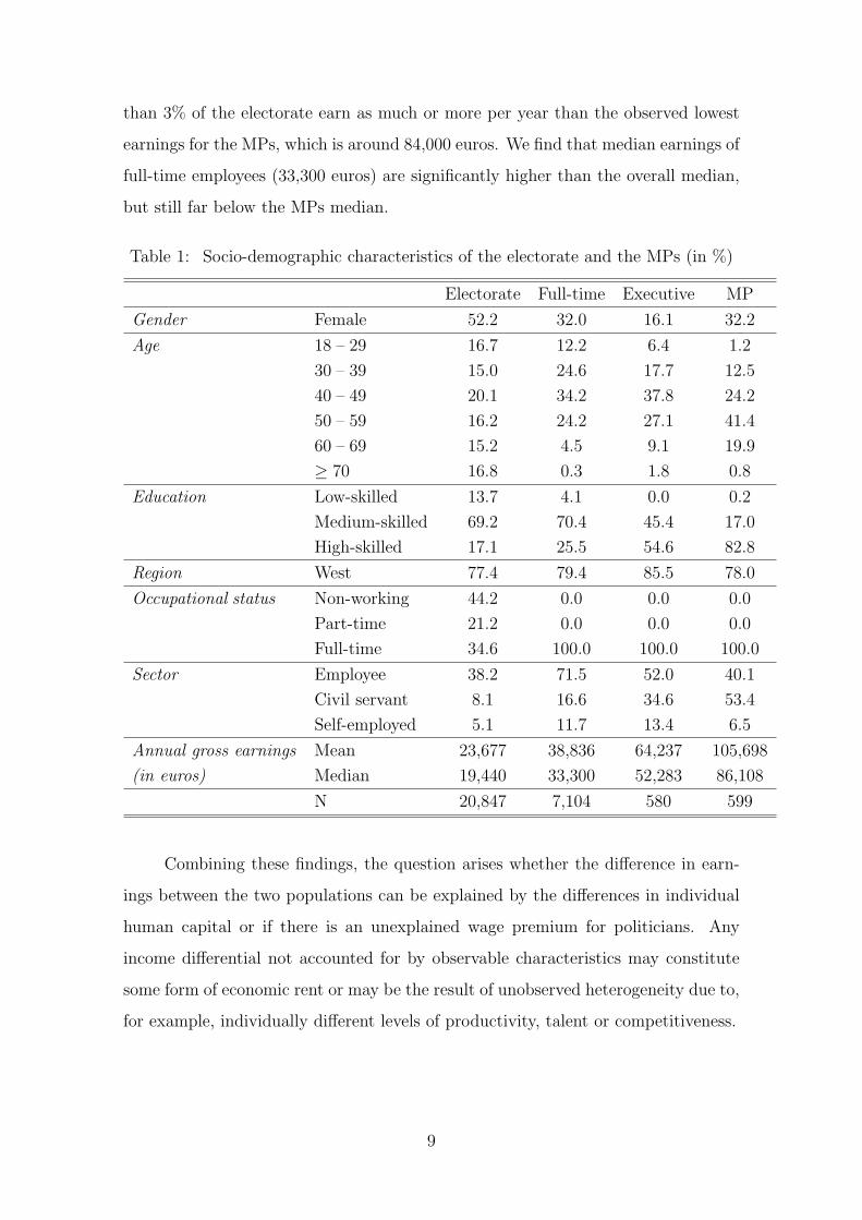
than 3% of the electorate earn as much or more per year than the observed lowest

earnings for the MPs, which is around 84,000 euros. We find that median earnings of

full-time employees (33,300 euros) are significantly higher than the overall median,

but still far below the MPs median.

Table 1: Socio-demographic characteristics of the electorate and the MPs (in %)

Electorate Full-time Executive MP

Gender Female 52.2 32.0 16.1 32.2

Age 18 – 29 16.7 12.2 6.4 1.2

30 – 39 15.0 24.6 17.7 12.5

40 – 49 20.1 34.2 37.8 24.2

50 – 59 16.2 24.2 27.1 41.4

60 – 69 15.2 4.5 9.1 19.9

≥ 70 16.8 0.3 1.8 0.8

Education Low-skilled 13.7 4.1 0.0 0.2

Medium-skilled 69.2 70.4 45.4 17.0

High-skilled 17.1 25.5 54.6 82.8

Region West 77.4 79.4 85.5 78.0

Occupational status Non-working 44.2 0.0 0.0 0.0

Part-time 21.2 0.0 0.0 0.0

Full-time 34.6 100.0 100.0 100.0

Sector Employee 38.2 71.5 52.0 40.1

Civil servant 8.1 16.6 34.6 53.4

Self-employed 5.1 11.7 13.4 6.5

Annual gross earnings Mean 23,677 38,836 64,237 105,698

(in euros) Median 19,440 33,300 52,283 86,108

N 20,847 7,104 580 599

Combining these findings, the question arises whether the difference in earn-

ings between the two populations can be explained by the differences in individual

human capital or if there is an unexplained wage premium for politicians. Any

income differential not accounted for by observable characteristics may constitute

some form of economic rent or may be the result of unobserved heterogeneity due to,

for example, individually different levels of productivity, talent or competitiveness.

9

4.2 Ordinary Least Squares

A Mincerian earnings equation is estimated using OLS regression, in which the

logarithmized annual gross earnings of individual i ∈ {1, ..., n} are defined as:

ln(Wi) = β0 + β1Pi + βXi + µi, (1)

with Pi a dummy variable of the value 1 if the individual is an MP and 0 otherwise. A

positive and significant estimator of β1 would provide empirical evidence in favor of

a wage premium for politicians. The vector Xi includes control variables which have

been identified in previous research to affect earnings such as gender, qualification

dummies, tenure (squared), dummies for being married, number of children, party

affiliation and executive position. Depending on the specification of the model, we

also include interaction terms of certain characteristics with the politician dummy

in order to test for heterogeneous effects. The error term is denoted by µi.

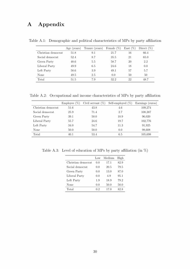
Baseline results. The unconditional earnings gap between MPs and citizens

working full-time is around 107%. This, however, might be due to differences in

observable characteristics (see Tables A.1–A.3 in the Appendix for distributions of

characteristics among MPs). Table 2 presents OLS results of the logarithmized

annual gross individual earnings on the key variable politician and a number of co-

variates that are known to affect income. Model 1 is estimated on the full sample

– defined as all individuals working full-time. We exclude non-working individuals

and part-time employees as they do not represent the desired comparison group in

order to identify the PWG.7 The results indicate a strong and positive effect of the

dummy variable politician, suggesting that MPs, ceteris paribus, earn 88% more

than non-MP citizens.

The covariate coefficients have the expected signs: tenure and age have a posi-

tive but decreasing effect on earnings.8 Education, which should also affect political

7 We also ran the regressions on a sample including part-timers as well as a part-time dummy.The estimated effects are almost identical to those of models 1 and 2.

8 While the variable tenure measures specific human capital (for politicians measured as yearsin the Bundestag and for the electorate as years in the current firm), age captures the remainingeffect of general human capital accumulation as a proxy variable of experience.

10

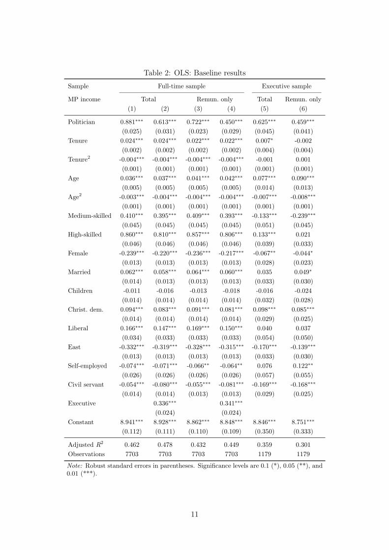
Table 2: OLS: Baseline results

Sample Full-time sample Executive sample

MP income Total Remun. only Total Remun. only(1) (2) (3) (4) (5) (6)

Politician 0.881∗∗∗ 0.613∗∗∗ 0.722∗∗∗ 0.450∗∗∗ 0.625∗∗∗ 0.459∗∗∗

(0.025) (0.031) (0.023) (0.029) (0.045) (0.041)Tenure 0.024∗∗∗ 0.024∗∗∗ 0.022∗∗∗ 0.022∗∗∗ 0.007∗ -0.002

(0.002) (0.002) (0.002) (0.002) (0.004) (0.004)Tenure2 -0.004∗∗∗ -0.004∗∗∗ -0.004∗∗∗ -0.004∗∗∗ -0.001 0.001

(0.001) (0.001) (0.001) (0.001) (0.001) (0.001)Age 0.036∗∗∗ 0.037∗∗∗ 0.041∗∗∗ 0.042∗∗∗ 0.077∗∗∗ 0.090∗∗∗

(0.005) (0.005) (0.005) (0.005) (0.014) (0.013)Age2 -0.003∗∗∗ -0.004∗∗∗ -0.004∗∗∗ -0.004∗∗∗ -0.007∗∗∗ -0.008∗∗∗

(0.001) (0.001) (0.001) (0.001) (0.001) (0.001)Medium-skilled 0.410∗∗∗ 0.395∗∗∗ 0.409∗∗∗ 0.393∗∗∗ -0.133∗∗∗ -0.239∗∗∗

(0.045) (0.045) (0.045) (0.045) (0.051) (0.045)High-skilled 0.860∗∗∗ 0.810∗∗∗ 0.857∗∗∗ 0.806∗∗∗ 0.133∗∗∗ 0.021

(0.046) (0.046) (0.046) (0.046) (0.039) (0.033)Female -0.239∗∗∗ -0.220∗∗∗ -0.236∗∗∗ -0.217∗∗∗ -0.067∗∗ -0.044∗

(0.013) (0.013) (0.013) (0.013) (0.028) (0.023)Married 0.062∗∗∗ 0.058∗∗∗ 0.064∗∗∗ 0.060∗∗∗ 0.035 0.049∗

(0.014) (0.013) (0.013) (0.013) (0.033) (0.030)Children -0.011 -0.016 -0.013 -0.018 -0.016 -0.024

(0.014) (0.014) (0.014) (0.014) (0.032) (0.028)Christ. dem. 0.094∗∗∗ 0.083∗∗∗ 0.091∗∗∗ 0.081∗∗∗ 0.098∗∗∗ 0.085∗∗∗

(0.014) (0.014) (0.014) (0.014) (0.029) (0.025)Liberal 0.166∗∗∗ 0.147∗∗∗ 0.169∗∗∗ 0.150∗∗∗ 0.040 0.037

(0.034) (0.033) (0.033) (0.033) (0.054) (0.050)East -0.332∗∗∗ -0.319∗∗∗ -0.328∗∗∗ -0.315∗∗∗ -0.170∗∗∗ -0.139∗∗∗

(0.013) (0.013) (0.013) (0.013) (0.033) (0.030)Self-employed -0.074∗∗∗ -0.071∗∗∗ -0.066∗∗ -0.064∗∗ 0.076 0.122∗∗

(0.026) (0.026) (0.026) (0.026) (0.057) (0.055)Civil servant -0.054∗∗∗ -0.080∗∗∗ -0.055∗∗∗ -0.081∗∗∗ -0.169∗∗∗ -0.168∗∗∗

(0.014) (0.014) (0.013) (0.013) (0.029) (0.025)Executive 0.336∗∗∗ 0.341∗∗∗

(0.024) (0.024)Constant 8.941∗∗∗ 8.928∗∗∗ 8.862∗∗∗ 8.848∗∗∗ 8.846∗∗∗ 8.751∗∗∗

(0.112) (0.111) (0.110) (0.109) (0.350) (0.333)

Adjusted R2 0.462 0.478 0.432 0.449 0.359 0.301Observations 7703 7703 7703 7703 1179 1179

Note: Robust standard errors in parentheses. Significance levels are 0.1 (*), 0.05 (**), and0.01 (***).

11

participation, has a positive effect on annual earnings. Compared to the low-skilled,

high-skilled (medium-skilled) individuals have a positive income differential of 86%

(41%). The female dummy reveals the well-known gender wage gap (Oaxaca, 1973)

– in our case of around 24%, which is comparable to previous estimates for Germany

(Kunze, 2005; Arulampalam, Booth, and Bryan, 2007). Being married slightly in-

creases income, but having children decreases it. The variables concerning party

affiliation confirm that members of those parties which are said to promote more

business friendly policies – Christian democrats (CDU/CSU) and FDP – have higher

levels of earnings (9% and 17% respectively). Living in East Germany reduces an-

nual gross individual earnings by 33% on average. Finally, employees in the private

sector have higher earnings than civil servants or self-employed.

In specification 2 we take into account that MPs by definition hold an executive

position in terms of occupation.9 They have personnel responsibility, which certainly

distinguishes them from the average employee. Moreover, we expect the executive

dummy to control for the fact members of the Bundestag – just as executives –

have climbed the job ladder within their respective profession. It also captures

the relatively high workload (and reduced leisure time) politicians and executives

experience. Finally, the inclusion of a variable controlling for an executive position

also enables us to address the common claim that politicians could earn much more

if they held a similar position in the private sector. Our results suggest that there is

no evidence for this claim. As expected, an executive position is associated with an

earnings premium and the politician coefficient decreases but remains positive and

significant, suggesting a wage premium of more than 60%. The covariate coefficients

hardly change.

In specifications 3 and 4 we use a different income definition for politicians.

Instead of estimating the models on total earnings, as was done in models 1 and

2, we assign MPs only the basic office remuneration – excluding outside earnings,

payments for cabinet members, pensions and interim allowances. While the coef-

ficients on the covariates are hardly affected, the ones on the politicians’ dummies

9 In the GSOEP, citizens are defined as executives when their occupational position is one ofthe following: master craftsman, self-employed with 10 or more employees, manager or executivecivil servant.

12

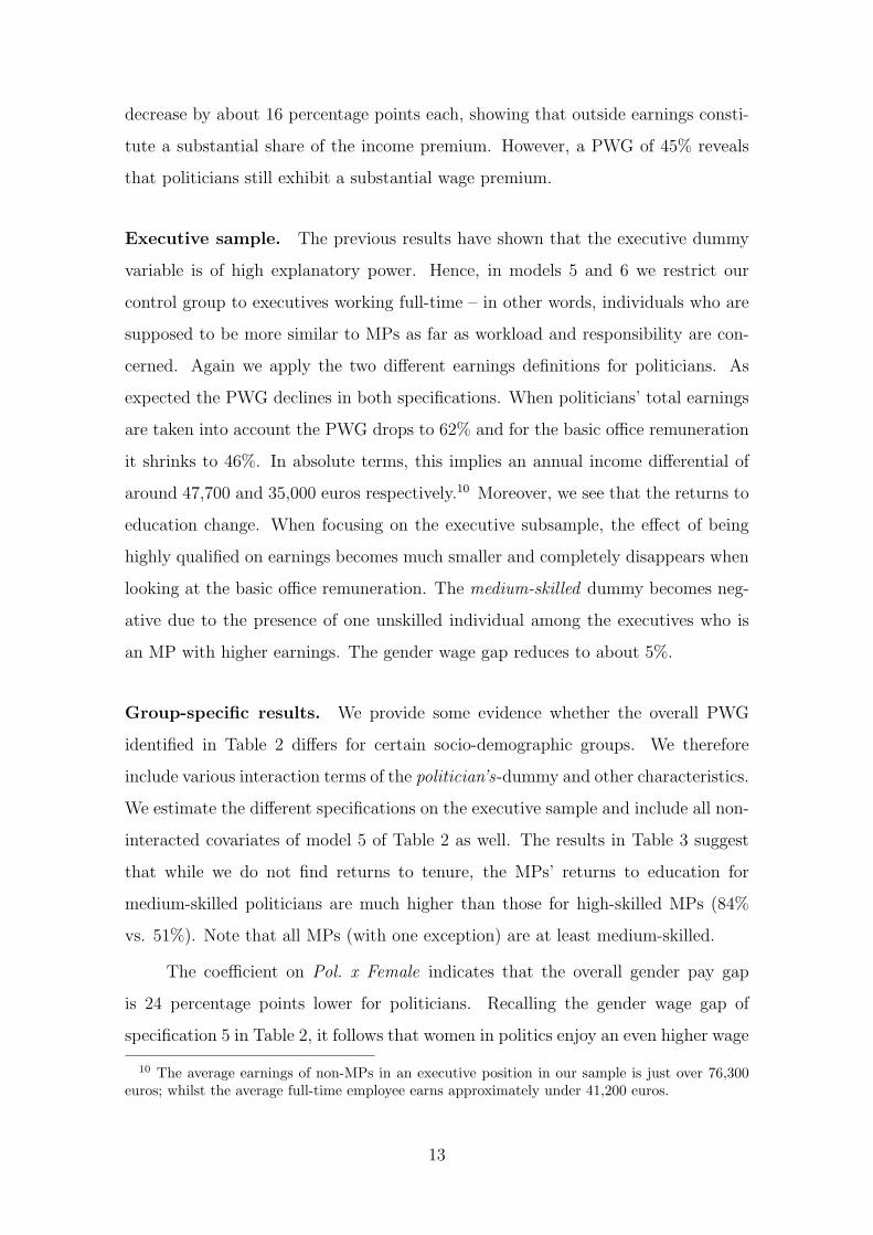
decrease by about 16 percentage points each, showing that outside earnings consti-

tute a substantial share of the income premium. However, a PWG of 45% reveals

that politicians still exhibit a substantial wage premium.

Executive sample. The previous results have shown that the executive dummy

variable is of high explanatory power. Hence, in models 5 and 6 we restrict our

control group to executives working full-time – in other words, individuals who are

supposed to be more similar to MPs as far as workload and responsibility are con-

cerned. Again we apply the two different earnings definitions for politicians. As

expected the PWG declines in both specifications. When politicians’ total earnings

are taken into account the PWG drops to 62% and for the basic office remuneration

it shrinks to 46%. In absolute terms, this implies an annual income differential of

around 47,700 and 35,000 euros respectively.10 Moreover, we see that the returns to

education change. When focusing on the executive subsample, the effect of being

highly qualified on earnings becomes much smaller and completely disappears when

looking at the basic office remuneration. The medium-skilled dummy becomes neg-

ative due to the presence of one unskilled individual among the executives who is

an MP with higher earnings. The gender wage gap reduces to about 5%.

Group-specific results. We provide some evidence whether the overall PWG

identified in Table 2 differs for certain socio-demographic groups. We therefore

include various interaction terms of the politician’s-dummy and other characteristics.

We estimate the different specifications on the executive sample and include all non-

interacted covariates of model 5 of Table 2 as well. The results in Table 3 suggest

that while we do not find returns to tenure, the MPs’ returns to education for

medium-skilled politicians are much higher than those for high-skilled MPs (84%

vs. 51%). Note that all MPs (with one exception) are at least medium-skilled.

The coefficient on Pol. x Female indicates that the overall gender pay gap

is 24 percentage points lower for politicians. Recalling the gender wage gap of

specification 5 in Table 2, it follows that women in politics enjoy an even higher wage

10 The average earnings of non-MPs in an executive position in our sample is just over 76,300euros; whilst the average full-time employee earns approximately under 41,200 euros.

13

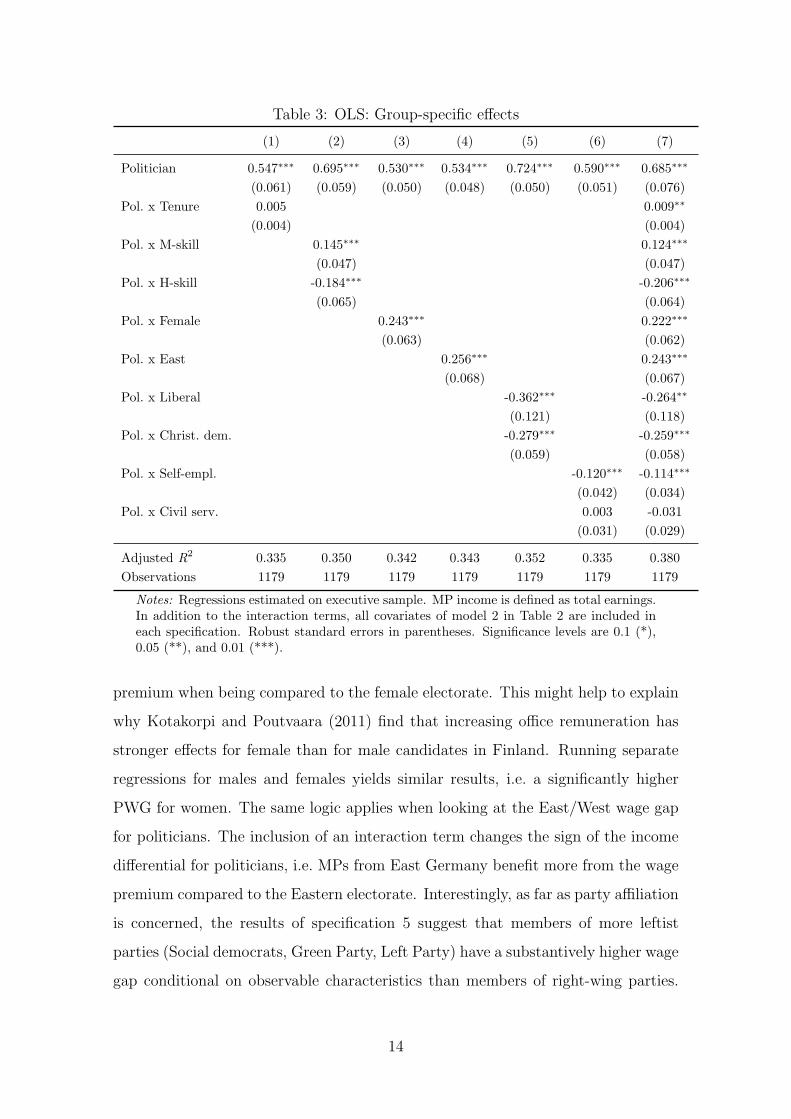
Table 3: OLS: Group-specific effects

(1) (2) (3) (4) (5) (6) (7)

Politician 0.547∗∗∗ 0.695∗∗∗ 0.530∗∗∗ 0.534∗∗∗ 0.724∗∗∗ 0.590∗∗∗ 0.685∗∗∗

(0.061) (0.059) (0.050) (0.048) (0.050) (0.051) (0.076)Pol. x Tenure 0.005 0.009∗∗

(0.004) (0.004)Pol. x M-skill 0.145∗∗∗ 0.124∗∗∗

(0.047) (0.047)Pol. x H-skill -0.184∗∗∗ -0.206∗∗∗

(0.065) (0.064)Pol. x Female 0.243∗∗∗ 0.222∗∗∗

(0.063) (0.062)Pol. x East 0.256∗∗∗ 0.243∗∗∗

(0.068) (0.067)Pol. x Liberal -0.362∗∗∗ -0.264∗∗

(0.121) (0.118)Pol. x Christ. dem. -0.279∗∗∗ -0.259∗∗∗

(0.059) (0.058)Pol. x Self-empl. -0.120∗∗∗ -0.114∗∗∗

(0.042) (0.034)Pol. x Civil serv. 0.003 -0.031

(0.031) (0.029)

Adjusted R2 0.335 0.350 0.342 0.343 0.352 0.335 0.380Observations 1179 1179 1179 1179 1179 1179 1179

Notes: Regressions estimated on executive sample. MP income is defined as total earnings.In addition to the interaction terms, all covariates of model 2 in Table 2 are included ineach specification. Robust standard errors in parentheses. Significance levels are 0.1 (*),0.05 (**), and 0.01 (***).

premium when being compared to the female electorate. This might help to explain

why Kotakorpi and Poutvaara (2011) find that increasing office remuneration has

stronger effects for female than for male candidates in Finland. Running separate

regressions for males and females yields similar results, i.e. a significantly higher

PWG for women. The same logic applies when looking at the East/West wage gap

for politicians. The inclusion of an interaction term changes the sign of the income

differential for politicians, i.e. MPs from East Germany benefit more from the wage

premium compared to the Eastern electorate. Interestingly, as far as party affiliation

is concerned, the results of specification 5 suggest that members of more leftist

parties (Social democrats, Green Party, Left Party) have a substantively higher wage

gap conditional on observable characteristics than members of right-wing parties.

14

More precisely, the earnings premium for liberal and Christian-democratic MPs

decreases to 36% and 45% respectively. Furthermore, the PWG is lower for MPs

who have been self-employed before becoming politician. In model 7 we control

for all interactions terms simultaneously and results do not change considerably. To

sum up, the PWG is higher for individuals who ceteris paribus have a lower earnings

potential in the private labor market.

Wage decomposition. We conduct a Oaxaca-Blinder type wage decomposition

to investigate to what extent the observed PWG can be explained by endowments

(Oaxaca, 1973; Blinder, 1973). Estimating the Mincerian earnings regression sepa-

rately for MPs and non-MPs allows difference in pay to be decomposed into a part

which is explained by observable characteristics – the covariates – and an unex-

plained part. The decomposition reveals that observable endowments such as skill

or age can only explain a negligible share of this difference for both samples and

earnings concepts (results available upon request). As the majority of the PWG

remains unexplained, we apply several matching techniques in Section 4.3 to further

investigate the PWG.

4.3 Matching

There are two main advantages of matching over simple OLS regression. First,

matching can be used to increase the comparability of the treated group – the politi-

cians – and the control group – the electorate. In addition to restricting the sample

as done in the OLS analysis, matching ensures that only the nearest neighbors in

terms of characteristics or the probability of receiving “treatment”, i.e. in our case

of becoming a politician, are used to estimate the PWG (Imbens, 2004; Imbens and

Wooldridge, 2009). In that sense, matching is comparable to non-parametric regres-

sion methods such as kernel estimation since it allows identification without explicit

assumptions regarding the (potentially non-linear) functional form of the association

between dependent variables and explanatory factors. Second, the matching frame-

work allows us to assess the relevance of potential unobserved factors influencing the

PWG. In the context of our study, this might be especially important as unobserved

15

motivation or assertiveness could explain parts of the PWG found in Section 4.2.

We define a binary “treatment” indicator Di ∈ {0, 1} that takes the value 1 if

an individual is an MP and 0 otherwise. Again, the outcome variable Wi(Di) is log

annual gross earnings. We are interested in estimating the average treatment effect

on the treated (ATT), which is defined as

τATT = E[W (1)|D = 1]− E[W (0)|D = 1] (2)

with E[.] standing for expectation. The ATT is equal to the potential income dif-

ferential if it was possible to draw an individual i randomly from the sample of MPs

only and allow the simultaneous pursue a career as an MP and as a non-MP citizen

in the regular labor market (see e.g. the survey by Caliendo and Kopeinig, 2008).

The choice of a profession in general and the career as a politician in particular

is an individual one (Gregory and Borland, 1999; Belman and Heywood, 1989).

Thus, it is critical to account for the factors that may have affected the choice

of occupation when estimating its effect on the level of earnings. Matching on

observable covariates X is an approach to solve this problem by finding “statistical

twins” in the treatment as well as in the control group. As matching on numerous

characteristics X might cause dimensionality problems, we follow standard practice

and condition on the propensity score of being treated instead. Rosenbaum and

Rubin (1983) show that propensity score matching equally ensures independence

of treatment assignment from the potential outcomes. We estimate the probability

of being a politician given X, P (D = 1|X), with a standard probit model. The

covariates X describe the self-selection into the treatment process and ensure that

ignorability of treatment is fulfilled. As a robustness check we also apply matching

on covariates using a Mahalanobis distance metric.

Rosenbaum bounds analysis. We have so far assumed that the observable co-

variates X fully account for the self-selection of individuals into treatment and con-

trol group. However, if there are unobserved factors that simultaneously affect

selection into treatment and the outcome, matching estimators are susceptible to a

hidden bias (Caliendo and Kopeinig, 2008). In the case of politicians, unobserved

16

characteristics, such as motivation, competitiveness or networking skills, might de-

termine selection into treatment, while simultaneously affecting earnings. To ac-

count for this potential bias, we follow Rosenbaum (2002) and examine whether the

estimated treatment effects are robust to the presence of unobserved confounding

variables.11 Assuming that besides observed covariates X an unobserved confounder

u exists, then the probability of receiving treatment for individual i is

πi = P (Xi, ui) = P (Di = 1|Xi, ui) = F (βXi + γui), (3)

where γ is the effect of ui on receiving the treatment (i.e. becoming an MP). Com-

paring the odds of a treated individual i to the odds of a matched individual j yields

the odds-ratio πi(1− πj)/πj(1− πi). Assuming that F is the logistic distribution,

Rosenbaum (2002) derives the following bounds for the odds-ratio

1

exp(γ)≤ πi(1− πj)

πj(1− πi)≤ exp(γ) ≡ Γ, (4)

where Γ measures the degree of departure from a situation without any hidden bias

(Γ = 1). The Wilcoxon sign rank test is applied to receive upper and lower bounds

of the significance level of the estimated treatment effect, given a certain value of Γ.

If this upper bound exceeds a certain threshold (5% in our case) for a given value

of Γ, we cannot reject the null that a potential confounding factor u, which has the

explanatory power of all observed covariates X times the value of Γ, renders the

estimated effects insignificant. In other words, low values of Γ (slightly greater than

1) indicate that results are sensitive to unobserved confounders; extreme values of Γ

(greater than 2.5) suggest that it is unlikely that confounding factors alter inference.

Matching results. We estimate the propensity score of being a politician using a

simple probit model with all the socio-demographic variables available in our data,

such as age, qualification, gender, children, marital status, occupational position

(for politicians before becoming MPs) and region. A balancing test of the propen-

11 Another estimation technique to account for unobserved heterogeneity is the application of afixed-effects regression (see Diermeier, Keane, and Merlo (2005) for an application to US Congressmembers). However, this would require a panel dataset of MPs, and we have only data for onelegislative period. Moreover, there is no variation in the politicians’ dummy for MPs.

17

sity score specification (Dehejia and Wahba, 2002) examines whether the estimated

propensity score is an adequate measure to ensure that the distribution of X is equal

among the control and treatment group at different values of the propensity score.12

As seen in Section 4.2 holding an executive position is an important factor when

estimating the PWG. We therefore restrict our control group to executives working

full-time. One of the main reasons for applying matching is that we want to make

politicians and citizens as comparable as possible. In this regard, the reduction of the

sample is not too costly since the explicit intention of the exercise is to consider only

good matches. Hence, we check whether there are significant differences between

treatment and control groups in the matched sample with regard to the means of

observable characteristics. We also report the mean standardized bias, which reveals

whether the matching was successful in balancing the covariates. We apply three

different matching algorithms and use two different earnings definitions (see above).

Table 4 presents the results of several propensity score matching models with

the logarithmized annual gross earnings as dependent variable. In specification 1

we employ a one-to-one nearest neighbor matching specification with replacement

and a caliper.13 The ATT for full earnings is highly significant and estimated at

0.397, which indicates that being a politician on average increases earnings by almost

40%.14 Moreover, the effect is very robust to unobserved confounders as indicated

by Rosenbaum’s Γ. The t-statistics show that matching on the propensity score

balances treatment and control group well, with no significant differences between

the groups after matching. It reduces 80–100% of the differences in observable

characteristics between politicians and the electorate. Also, a standardized bias of

under 3 suggests that matching was successful (Caliendo and Kopeinig, 2008).

12 Following Dehejia and Wahba (2002) we sequentially add higher order terms of the covariatesas well as interactions of those variables to the model until the balancing property is satisfied(Rubin and Thomas, 2000). Note that the interpretation of the coefficients of the propensity scoreestimation is not economically relevant. Neither is the purpose of propensity score estimation topredict the selection into treatment, but to balance the covariates. For completeness, estimationresults of the probit estimation are presented in Table A.4 in the Appendix.

13 Following Rosenbaum and Rubin (1985), a caliper of one quarter of the standard deviation ofthe estimated propensity score is chosen.

14 For model 1 the standard error is calculated using the correction proposed by Abadie andImbens (2006) for nearest neighbor with replacement on a continuous covariate. Note that we donot find significant differences between the ATT and the average treatment effect in any of thethree models.

18

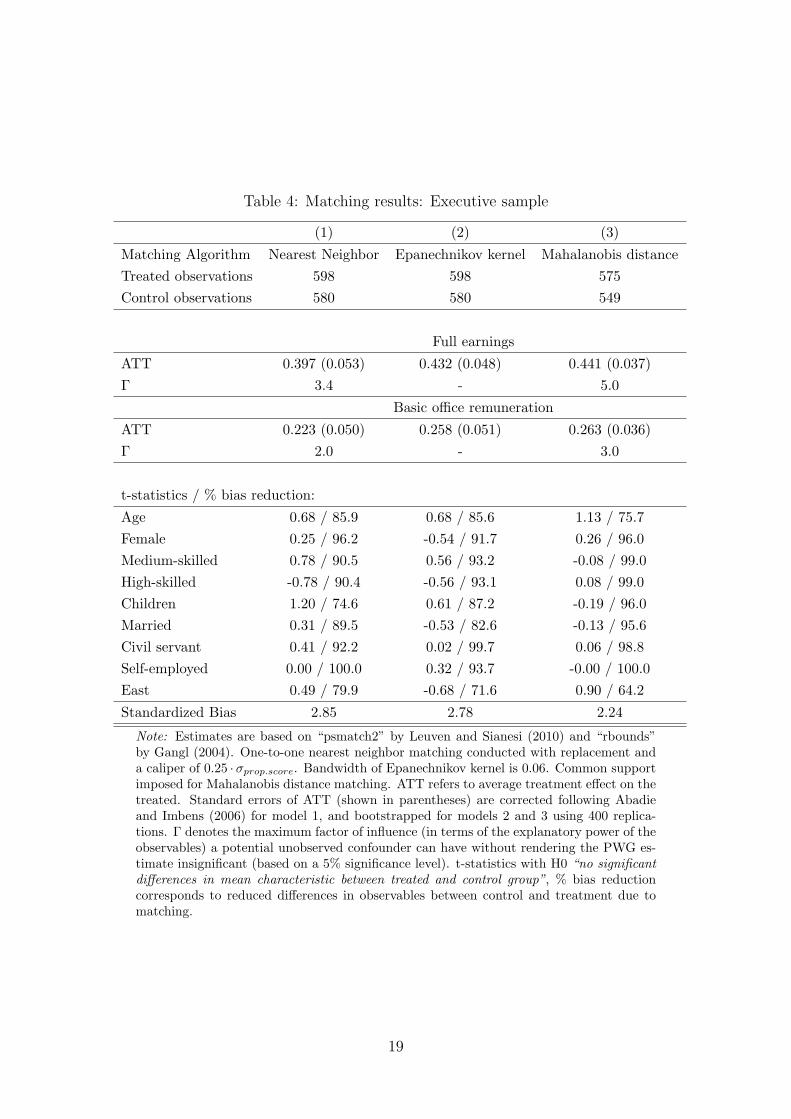
Table 4: Matching results: Executive sample

(1) (2) (3)

Matching Algorithm Nearest Neighbor Epanechnikov kernel Mahalanobis distanceTreated observations 598 598 575Control observations 580 580 549

Full earnings

ATT 0.397 (0.053) 0.432 (0.048) 0.441 (0.037)Γ 3.4 - 5.0

Basic office remuneration

ATT 0.223 (0.050) 0.258 (0.051) 0.263 (0.036)Γ 2.0 - 3.0

t-statistics / % bias reduction:

Age 0.68 / 85.9 0.68 / 85.6 1.13 / 75.7Female 0.25 / 96.2 -0.54 / 91.7 0.26 / 96.0Medium-skilled 0.78 / 90.5 0.56 / 93.2 -0.08 / 99.0High-skilled -0.78 / 90.4 -0.56 / 93.1 0.08 / 99.0Children 1.20 / 74.6 0.61 / 87.2 -0.19 / 96.0Married 0.31 / 89.5 -0.53 / 82.6 -0.13 / 95.6Civil servant 0.41 / 92.2 0.02 / 99.7 0.06 / 98.8Self-employed 0.00 / 100.0 0.32 / 93.7 -0.00 / 100.0East 0.49 / 79.9 -0.68 / 71.6 0.90 / 64.2

Standardized Bias 2.85 2.78 2.24

Note: Estimates are based on “psmatch2” by Leuven and Sianesi (2010) and “rbounds”by Gangl (2004). One-to-one nearest neighbor matching conducted with replacement anda caliper of 0.25 · σprop.score. Bandwidth of Epanechnikov kernel is 0.06. Common supportimposed for Mahalanobis distance matching. ATT refers to average treatment effect on thetreated. Standard errors of ATT (shown in parentheses) are corrected following Abadieand Imbens (2006) for model 1, and bootstrapped for models 2 and 3 using 400 replica-tions. Γ denotes the maximum factor of influence (in terms of the explanatory power of theobservables) a potential unobserved confounder can have without rendering the PWG es-timate insignificant (based on a 5% significance level). t-statistics with H0 “no significantdifferences in mean characteristic between treated and control group”, % bias reductioncorresponds to reduced differences in observables between control and treatment due tomatching.

19

In specification 2 we use an Epanechnikov kernel matching estimator. This

estimator makes use of all observations and weighs them according to their distance

in the propensity score. Thus, we trade more efficiency for a potentially higher bias

of our estimates as we do not restrict the analysis to the best matches. In fact,

treatment effects hardly change in size and remain highly significant.15 Again, all

covariates of the model are balanced and the bias reduction is similar to model 1.

In model 3 we use matching on covariates based on the Mahalanobis distance

metric to estimate treatment effects.16 As an alternative to caliper matching, we

introduce common support to guarantee that only good matches are taken into

consideration. As a consequence, the number of individuals used for matching is

slightly reduced, increasing the variance of the estimates. Reassuringly, the ATT

does not change much and remains highly significant.

The estimated effects shrink considerably, when we make use of a different

income definition. With basic office remuneration – excluding outside earnings,

payments for cabinet members, pensions and interim allowances – the ATT drops

by about 40%, underpinning once again the importance of outside earnings when

looking at the PWG. In spite of this decline, the treatment effects are still signifi-

cantly different from zero and have a substantial magnitude. For instance, a PWG

of 25.8%, as estimated for model 2, implies an average annual wage premium of

about 20,000 euros compared to 33,000 euros for the full earnings specification.

5 Discussion of the Results

Robustness. The existence of a sizeable PWG is robust to the estimation tech-

nique (OLS vs. matching), various specifications, control groups, earnings definitions

and unobserved heterogeneity. As far as matching is concerned, we obtain similar

results when using a logit instead of a probit model to estimate the propensity score.

Moreover, reducing the complexity of the binary dependent variable model by ex-

15 For models 2 and 3 we bootstrap standard errors using 400 replications. Note that a Rosen-baum bound analysis cannot be performed when a kernel matching estimator is employed.

16 We include all covariates shown in the bottom part of Table 4 and the propensity score tocalculate the Mahalanobis distance.

20

cluding higher-order and interactions terms does not affect the results. Neither does

the introduction of common support – instead of a caliper – change our findings.

Moreover, the matching results are robust with respect to different kernels.

We additionally check the robustness of our estimates by changing the defi-

nition of the control group.17 First, we exclude public sector employees from our

executive sample, since they have fixed wage trajectories and no performance based

paying scheme. The PWG decreases to 14–40% (12,000–34,000 euros p.a.) for full

earnings. Further narrowing the executive definition to “managers” only reduces

the PWG to 18–30% (18,000–32,000 euros p.a.). In both cases, the PWG remains

sizeable and significant ruling out that the private-public sector wage gap or the

choice of the control group drives the average PWG for full earnings. Results for

basic office remuneration vary between 0 and 25%. However, the control group of

managers is representative for the total population, whereas top managers of large,

multinational enterprizes are very rare. In fact, there are only two individuals in our

data with annual labor earnings exceeding one million euros. Hence, the PWG we

measure differs from the publicly perceived wage gap between politicians and top

executives. Defining the control group as the upper 5% of the earnings distribution

yields a PWG of 10–16% for full MP earnings (corresponding to 10,000–16,000 euros

p.a.) while it vanishes and turns negative when considering office remuneration only.

Size of the effects. Besides being robust, the estimated PWG is highly significant

and substantial in size. Nevertheless, we argue that our findings are lower bound

estimates for two reasons. First, the data on earnings of MPs are close to a lower

bound themselves, since we can only rely on information on outside earnings that

are reported in broader income classes. As we assume a conservative upper bound

of outside earnings, our estimated effects will rather be biased downwards (Becker,

Peichl, and Rincke, 2009). Second, one can distinguish two main types of MPs:

career politicians vs. political careers (Mattozzi and Merlo, 2008). While politicians

of the first type typically remain in office until retirement, representatives pursuing

a political career resign from office before retirement age and change to the private

17 See Table A.5 for an overview of PWG estimates for different control groups.

21

sector (again). It it plausible that having been in office as MP for a couple of years

creates more attractive job opportunities, ceteris paribus. It might be exactly this

mechanism that leads to the widely held belief that politicians earn more in the

private sector. For instance, a career as an MP brings along many occasions to

socialize with potential employers.18 This can be interpreted as a non-monetary

benefit of political office, which can translate into a monetary one after leaving the

political arena. Hence, the true “lifetime PWG” would be higher.

An argument in favor of a positive PWG could be additional non-monetary

costs. MPs have to work their way up for many years before becoming career

politicians which requires effort. In addition, the rather low reputation of politicians

in general (see above), the loss of privacy or job-insecurity because of elections reduce

the attractiveness of the job. However, one has to take into account that there are

also non-monetary benefits of being in office, such as satisfying the desire for power

or having the possibility to implement policies in accordance with one’s convictions.

Both non-monetary costs and benefits are not measurable and hence not further

investigated here – implicitly assuming that they balance each other.

Our results are based on gross earnings before taxes which is the common

income definition in the labor economics literature on wage gaps. The question

arises whether the PWG would turn out to be different for disposable income after

taxes. Unfortunately, we do not observe all the relevant information for MPs in

order to calculate tax liabilities. Therefore, we can only speculate that the PWG

should not change much due to two opposing effects. On the one hand, MPs ceteris

paribus pay higher taxes because of progressive income taxation in Germany. On

the other hand, it is well-known that German MPs donate larger amounts to their

parties which are deductable from the income tax liability. Hence, the sign of the

net-effect is unclear.

Campaigning costs. Even after accounting for observed as well as unobserved

characteristics, we still find a substantial earnings premium for politicians. However,

as laid out in Section 2, the citizen candidate framework provides a justification for

18 In addition, there is a relatively recent literature on the returns to being a politician (Eggersand Hainmueller, 2009; Querubin and Snyder, 2009) which is more concerned with lifetime income.

22

a PWG. Individuals of high ability, and hence with above average earnings poten-

tial in the private sector, will only decide to run for office when the remuneration

compensates for campaigning costs. Hence, the detected wage premium could be

justifiable if the amount of politicians’ surplus earnings equaled their campaigning

costs. Figuring out whether this holds true in the case of Germany would require

detailed information on individual campaigning activities and their costs in terms

of both monetary costs and time devoted to the campaign.19 Unfortunately, this

information is not available for German MPs. Nevertheless, in a back of the en-

velope calculation, we make an attempt to approximate the costs of campaigning

and compare them to our findings for the PWG. There is suggestive evidence that

monetary campaigning costs for German MPs total 30,000 to 65,000 euros (for a

four-year legislative term).20 Hence, only part of the detected earnings premium

can be justified by monetary campaigning costs, since the PWG in absolute terms

is estimated to lie between 100,000 and 190,000 euros (over a period of four years),

depending on the specification.

Normative implications. One can think of several potential explanations for the

existence of a PWG exceeding the threshold of campaigning costs: First, the PWG

can be thought of as a compensation for unobserved characteristics, since elected

politicians can be assumed to be more talented or more motivated. However, the

Rosenbaum bounds analysis does not support this view as the unobserved factor

(for the executive sample) must be 3 to 5 times larger than the effects of all observ-

ables together – which is unlikely given our set of covariates. A second explanation

emphasizes the politicians’ above average workload. Many German MPs usually

state to work 50–70 hours a week (exact information on working hours of MPs is

19 For effects of campaign spending on election outcomes see Gerber (1998) and Evans (2007).20 In order to calculate these numbers, we divide the total campaigning expenses of the five

parties represented in the Bundestag in 2005 (61 million euros at the federal level and 125million euros in total) by the number of candidates (1,912). We also refer to information oncampaigning costs voluntarily disclosed by two MPs on their personal websites, which revealsimilar magnitudes (Martin Dormann: http://www.martin-doermann.de/live/wp-content/uploads/2008/02/glaeserne-taschen.pdf (01–14–2011) and Florian Pronold: http://www.glaeserner-abgeordneter.de/infotour/wahlkampfausgaben (01–14–2011)). On the individ-ual level, these costs include de facto mandatory donations of MPs to their respective parties(“Mandatstragerbeitrage”).

23

not available) and one could argue that the extra pay for politicians compensates

for less leisure time. However, compared to the average working hours of a full-time

executive which is 55 hours a week (the top 10% on average work 74 hours), one

can conclude that the high workload is not exceptional given the MPs’ position.

Hence, the PWG we find for the executive sample remains unchallenged by this

claim. Finally, politicians might extract rents from being in office: MPs in Germany

and several other countries decide themselves on the level of office remuneration.

6 Conclusions

In this paper we show the existence of a PWG for German MPs after conditioning

on relevant wage determinants. Both OLS and matching analyses reveal a signifi-

cant and substantial wage premium for MPs, which varies between 70–90% for the

full sample and between 40–60% (corresponding to 30,000–50,000 euros per year)

when restricting the control group to citizens in executive positions with a similar

workload. Hence, we show that the claim that politicians would earn significantly

more when working in the private sector is not confirmed by our data – in fact,

the opposite is true. The income premium is reduced to 20–45% (corresponding

to 17,000–35,000 euros per year) when focusing on the basic office remuneration,

i.e. excluding politicians’ outside earnings, but remains both economically and sta-

tistically significant. In addition, the Rosenbaum bounds analysis reveals that the

significance of the wage gap is unlikely to be caused by unobserved factors.

We further show that the PWG exceeds reasonable estimates of campaigning

costs and cannot be justified by extraordinary workload of MPs. If the general

perception of the electorate is that politicians do not meet their job’s above average

responsibility, the above average pay might consequently pose a threat not only to

the legitimacy of the politicians, but also to the acceptance of democracy in general.

This problem might even be aggravated in the light of theoretical and empirical

studies showing that higher earnings need not necessarily lead to better politicians

(Poutvaara and Takalo, 2007; Kotakorpi and Poutvaara, 2011). As far as our results

are concerned, we cannot refute the claim that (part) of the PWG can be seen as

24

rent extraction which hurts voters. This would call for a reform of the German

system of remuneration of MPs – especially with respect to the legal framework of

outside earnings, which account for 30–40% of the PWG.21

Since our analysis focuses on Germany, the question arises whether the main

findings are likely to apply to other countries as well. With its socio-economic

and demographic structure, Germany can be seen as a typical Western European

democracy. However, the institutional details and regulations on outside earnings

are rather special. Therefore, more (comparative) country studies are required to

complete the picture.

References

Abadie, A., and G. W. Imbens (2006): “Large Sample Properties of MatchingEstimators for Average Treatment Effects,” Econometrica, 74(1), 235–267.

Allensbacher Archiv (2008): “IfD-Umfragen 10015,” Institut fur DemoskopieAllensbach.

Arulampalam, W., A. L. Booth, and M. L. Bryan (2007): “Is there a GlassCeiling over Europe? Exploring the Gender Pay Gap across the Wage Distribu-tion,” Industrial and Labor Relations Review, 60(2), 163–186.

Atkinson, A. B., and T. Piketty (2007): Top Incomes over the TwentiethCentury. Oxford University Press, Oxford.

Bach, S., G. Corneo, and V. Steiner (2009): “From Bottom to Top: The En-tire Income Distribution in Germany, 1992–2003,” Review of Income and Wealth,55(2), 303–330.

Becker, J., A. Peichl, and J. Rincke (2009): “Politicians’ Outside Earningsand Electoral Competition,” Public Choice, 140(3–4), 379–394.

Belman, D., and J. S. Heywood (1989): “Government Wage Differentials: ASample Selection Approach,” Applied Economics, 21(4), 427–439.

Bender, K. A. (1998): “The Central Government-Private Wage Differential,”Journal of Economic Surveys, 12(2), 177–220.

Besley, T. (2004): “Joseph Schumpeter Lecture: Paying Politicians: Theory andEvidence,” Journal of the European Economic Association, 2(2–3), 193–215.

21 Note that in contrast to the US, where outside income for MPs is limited to 15% of the payfor Level II of the Executive Schedule, outside earnings in Germany are not limited. Furthermore,Gagliarducci, Nannicini, and Naticchioni (2010) find a positive association between outside earningsand absenteeism. In addition, politicians might be influenced or even become financially dependenton certain lobby groups because of outside income (Couch, Atkinson, and Shugart II, 1992).

25

Besley, T., and S. Coate (1997): “An Economic Model of RepresentativeDemocracy,” Quarterly Journal of Economics, 112(1), 85–114.

Blank, R. M. (1993): “Public Sector Growth and Labor Market Flexibility: TheUnited States vs. The United Kingdom,” National Bureau of Economic ResearchWorking Paper No. 4339.

Blinder, A. S. (1973): “Wage Discrimination: Reduced Form and StructuralEstimates,” Journal of Human Resources, 8(4), 436–455.

Bobo, L., and F. D. Gilliam Jr. (1990): “Race, Sociopolitical Participation,and Black Empowerment,” American Political Science Review, 84(2), 377–393.

Braendle, T., and A. Stutzer (2010): “Public Servants in Parliament: Theoryand Evidence on its Determinants in Germany,” Public Choice, 145(1–2), 223–252.

Bundesministergesetz (2008): “Gesetz uber die Rechtsverhaltnisse der Mit-glieder der Bundesregierung,” Bundesgesetzblatt I, S. 2018.

Bundestag (2009): “Entwurf eines Siebenundzwanzigsten Gesetzes zur Anderungdes Abgeordnetengesetzes,” Deutscher Bundestag, Drucksache 16/6924, Heene-man, Berlin.

(2010): “Verhaltensregeln fur Mitglieder des Deutschen Bundestages,”Deutscher Bundestag, Geschaftsordnung des Deutschen Bundestages undGeschaftsordnung des Vermittlungsausschusses.

(2011): “Hinweise zur Veroffentlichung der Angaben gemaß Verhal-tensregeln im Amtlichen Handbuch und auf den Internetseiten des DeutschenBundestages,” Deutscher Bundestag, http://www.bundestag.de/bundestag/

abgeordnete17/nebentaetigkeit/hinweise17.html.

Cadigan, J. (2005): “The Citizen Candidate Model: An Experimental Analysis,”Public Choice, 123(1–2), 197–216.

Caliendo, M., and S. Kopeinig (2008): “Some Practical Guidance for the Imple-mentation of Propensity Score Matching,” Journal of Economic Surveys, 22(1),31–72.

Caselli, F., and M. Morelli (2004): “Bad Politicians,” Journal of Public Eco-nomics, 88(3–4), 759–782.

Couch, J. F., K. E. Atkinson, and W. F. Shugart II (1992): “EthicLaws and the Outside Earnings of Politicians: The Case of Alabam’s “legislator-educators”,” Public Choice, 73(2), 135–145.

De Paola, M., and V. Scoppa (2011): “Political Competition and PoliticianQuality: Evidence from Italian Municipalities,” Public Choice, forthcoming.

Dehejia, R. H., and S. Wahba (2002): “Propensity Score-Matching Methodsfor Nonexperimental Causal Studies,” Review of Economics and Statistics, 84(1),151–161.

26

Diermeier, D., M. Keane, and A. Merlo (2005): “A Political Economy Modelof Congressional Careers,” American Economic Review, 95(1), 347–373.

Downs, A. (1957): An Economic Theory of Democracy. Harper and Brothers, NewYork.

Eggers, A. C., and J. Hainmueller (2009): “MPs for Sale? Estimating Returnsto Office in Postwar British Politics,” American Political Science Review, 103(4),513–533.

Ehrenberg, R. G., and J. L. Schwarz (1987): “Public Sector Labor Markets,”in Handbook of Labor Economics, Volume 2, ed. by O. Oshenfelter, and D. Card.North-Holland, Amsterdam.

European Social Survey (2007): Exploring Public Attitudes, Informing PublicPolicy: Selected Findings from the First Three Rounds.

Evans, T. (2007): “An Empirical Test of Why Incumbents Adopt Campaign Spend-ing Limits,” Public Choice, 132(3), 437–456.

Ferraz, C., and F. Finan (2009): “Motivating Politicians: The Impact of Mon-etary Incentives on Quality and Performance,” National Bureau of Economic Re-search Working paper No. 14906.

Freeman, R. B. (1986): “Unionism Comes to the Public Sector,” Journal ofEconomic Literature, 24(1), 41–86.

Frick, J. R., J. Goebel, M. M. Grabka, O. Groh-Samberg, and G. G.Wagner (2007): “Zur Erfassung von Einkommen und Vermogen in Haushaltssur-veys: Hocheinkommensstichprobe und Vermogensbilanz im SOEP,” SOEPpaperon Multidisciplinary Panel Data Research No. 19, German Institute for EconomicResearch (DIW) Berlin.

Gagliarducci, S., and T. Nannicini (2009): “Do Better Paid Politicians Per-form Better? Disentangling Incentives from Selection,” IZA Discussion PaperNo. 4400.

Gagliarducci, S., T. Nannicini, and P. Naticchioni (2010): “MoonlightingPoliticians,” Journal of Public Economics, 94(9–10), 688–699.

Gangl, M. (2004): “RBOUNDS: Stata Module to Perform Rosenbaum Sensitiv-ity Analysis for Average Treatment Effects on the Treated,” Statistical SoftwareComponents, Boston College Department of Economics.

Gerber, A. (1998): “Estimating the Effect of Campaign Spending on Senate Elec-tion Outcomes Using Instrumental Variables,” American Political Science Review,92(2), 401–411.

Gersbach, H. (2009): “Competition of Politicians for Wages and Office,” SocialChoice and Welfare, 33(1), 51–71.

27

Gilens, M. (2005): “Inequality and Democratic Responsiveness,” Public OpinionQuarterly, 69(5), 778–796.

Gorodnichenko, Y., and K. S. Peter (2007): “Public Sector Pay and Corrup-tion: Measuring Bribery from Micro Data,” Journal of Public Economics, 91(5-6),963–991.

Gregory, R. G., and J. Borland (1999): “Recent Developments in Public La-bor Markets,” in Handbook of Labor Economics, Volume 3c, ed. by O. Oshenfelter,and D. Card. North-Holland, Amsterdam.

Hartog, J., and H. Oosterbeek (1993): “Public and private sector wages inthe Netherlands,” European Economic Review, 37(1), 97–114.

Hay, C. (2007): Why We Hate Politics. Polity Press, Cambridge.

Imbens, G. W. (2004): “Nonparametric Estimation of Average Treatment EffectsUnder Exogeneity: A Review,” Review of Economics and Statistics, 86(1), 4–29.

Imbens, G. W., and J. M. Wooldridge (2009): “Recent Developments in theEconometrics of Program Evaluation,” Journal of Economic Literature, 47(1),5–86.

Kotakorpi, K., and P. Poutvaara (2011): “Pay for Politicians and CandidateSelection: An Empirical Analysis,” Journal of Public Economics, forthcoming.

Kunze, A. (2005): “The Evolution of the Gender Wage Gap,” Labour Economics,12(1), 73–97.

Leuven, E., and B. Sianesi (2010): “PSMATCH2: Stata Module to Perform FullMahalanobis and Propensity Score Matching, Common Support Graphing, andCovariate Imbalance Testing,” Statistical Software Components, Boston CollegeDepartment of Economics.

Lineberry, R. L. (1978): “Reform, Representation, and Policy,” Social ScienceQuarterly, 59(1), 173–177.

Mattozzi, A., and A. M. Merlo (2008): “Political Careers or Career Politi-cians?,” Journal of Public Economics, 92(3–4), 597–608.

Meier, K. J., and R. E. England (1984): “Black Representation and Edu-cational Policy: Are They Related?,” American Political Science Review, 78(2),392–403.

Melly, B. (2005): “Private Sector Wage Differentials in Germany: Evidence fromQuantile Regression,” Empirical Economics, 30(2), 505–520.

Messner, M., and M. K. Polborn (2004): “Paying Politicians,” Journal ofPublic Economics, 88(12), 2423–2445.

Oaxaca, R. (1973): “Male-Female Wage Differentials in Urban Labor Markets,”International Economic Review, 14(3), 693–709.

28

Osborne, M. J., and A. Slivinski (1996): “A Model of Political Competitionwith Citizen-Candidates,” Quarterly Journal of Economics, 111(1), 65–96.

Pederson, P. J., J. B. Schmidt-Sørensen, N. Smith, and N. Westergard-Nielsen (1990): “Wage Differentials Between the Public and Private Sectors,”Journal of Public Economics, 41(1), 125–145.

Pitkin, H. F. (1972): The Concept of Representation. University of CaliforniaPress, Berkeley.

Poutvaara, P., and T. Takalo (2007): “Candidate Quality,” International Taxand Public Finance, 14(1), 7–27.

Querubin, P., and J. M. Snyder (2009): “The Returns to US CongressionalSeats in the Mid-19th Century,” in The Political Economy of Democracy, ed. byE. Aragones, C. Bevia, H. Llavador, and N. Schofield. BBVA, Bilbao.

Roine, J., J. Vlachos, and D. Waldenstrom (2009): “The Long-Run Deter-minants of Inequality: What can we learn from Top Incoem Data?,” Journal ofPublic Economics, 93(7–8), 974–988.

Roine, J., and D. Waldenstrom (2008): “The Evolution of Top Incomes on anEgalitarian Society: Sweden, 1903–2004,” Journal of Public Economics, 92(1–2),366–387.

Rosenbaum, P. R. (2002): Observational Studies. Springer, New York, 2. edn.

Rosenbaum, P. R., and D. B. Rubin (1983): “The Central Role of the PropensityScore in Observational Studies for Causal Effects,” Biometrika, 70(1), 41–55.

(1985): “Constructing a Control Group Using Multivariate Matched Sam-pling Methods That Incorporate the Propensity Score,” American Statistician,39(1), 33–38.

Rubin, D. B., and N. Thomas (2000): “Combining Propensity Score Matchingwith Additional Adjustments for Prognostic Covariates,” Journal of the AmericanStatistical Association, 95(450), 573–585.

Solt, F. (2008): “Economic Inequality and Democratic Political Engagement,”American Journal of Political Science, 52(1), 48–60.

Wagner, G. G., J. R. Frick, and J. Schupp (2007): “The German Socio-economic Panel Study (SOEP): Scope, Evolution and Enhancements,” SchmollersJahrbuch, 127(1), 139–169.

29

A Appendix

Table A.1: Demographic and political characteristics of MPs by party affiliation

Age (years) Tenure (years) Female (%) East (%) Direct (%)

Christian democrat 51.8 9.1 21.7 16 66.4

Social democrat 52.4 8.7 35.5 21 65.0

Green Party 48.6 5.5 58.7 20 2.2

Liberal Party 49.9 6.5 24.6 18 0.0

Left Party 50.6 3.9 49.1 57 5.7

None 49.5 2.5 0.0 50 50

Total 51.5 7.9 32.2 22 48.7

Table A.2: Occupational and income characteristics of MPs by party affiliation

Employee (%) Civil servant (%) Self-employed (%) Earnings (euros)

Christian democrat 51.6 43.8 4.6 109,274

Social democrat 25.9 71.4 2.7 108,387

Green Party 39.1 50.0 10.9 96,020

Liberal Party 55.7 24.6 19.7 102,776

Left Party 34.0 54.7 11.3 91,925

None 50.0 50.0 0.0 98,608

Total 40.1 53.4 6.5 105,698

Table A.3: Level of education of MPs by party affiliation (in %)

Low Medium High

Christian democrat 0.0 17.1 82.9

Social democrat 0.0 20.5 79.5

Green Party 0.0 13.0 87.0

Liberal Party 0.0 4.9 95.1

Left Party 1.9 18.9 79.2

None 0.0 50.0 50.0

Total 0.2 17.0 82.8

30

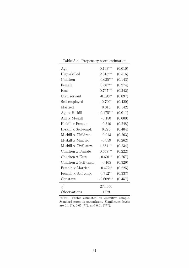
Table A.4: Propensity score estimation

Age 0.193∗∗∗ (0.010)

High-skilled 2.315∗∗∗ (0.516)

Children -0.635∗∗∗ (0.143)

Female 0.587∗∗ (0.274)

East 0.767∗∗∗ (0.242)

Civil servant -0.198∗∗ (0.097)

Self-employed -0.790∗ (0.420)

Married 0.016 (0.142)

Age x H-skill -0.175∗∗∗ (0.011)

Age x M-skill -0.150 (0.000)

H-skill x Female -0.310 (0.248)

H-skill x Self-empl. 0.276 (0.404)

M-skill x Children -0.013 (0.263)

M-skill x Married -0.059 (0.262)

M-skill x Civil serv. 1.584∗∗∗ (0.234)

Children x Female 0.657∗∗∗ (0.222)

Children x East -0.601∗∗ (0.267)

Children x Self-empl. -0.165 (0.329)

Female x Married -0.472∗∗ (0.225)

Female x Self-emp. 0.712∗∗ (0.337)

Constant -2.609∗∗∗ (0.457)

χ2 274.650

Observations 1179

Notes: Probit estimated on executive sample.Standard errors in parentheses. Significance levelsare 0.1 (*), 0.05 (**), and 0.01 (***).

31

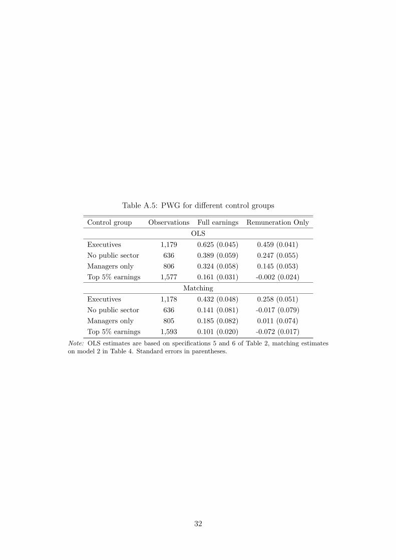
Table A.5: PWG for different control groups

Control group Observations Full earnings Remuneration Only

OLS

Executives 1,179 0.625 (0.045) 0.459 (0.041)No public sector 636 0.389 (0.059) 0.247 (0.055)Managers only 806 0.324 (0.058) 0.145 (0.053)Top 5% earnings 1,577 0.161 (0.031) -0.002 (0.024)

Matching

Executives 1,178 0.432 (0.048) 0.258 (0.051)No public sector 636 0.141 (0.081) -0.017 (0.079)Managers only 805 0.185 (0.082) 0.011 (0.074)Top 5% earnings 1,593 0.101 (0.020) -0.072 (0.017)

Note: OLS estimates are based on specifications 5 and 6 of Table 2, matching estimateson model 2 in Table 4. Standard errors in parentheses.

32