Embed Size (px)
Citation preview
The Potential and Limits of Digital
Election Forensics
�Jozef Janovsky
Keble College
University of Oxford
A dissertation submitted in partial fulfilment of the requirements for the
degree of Master of Science in Applied Statistics
13 September 2013

This thesis is dedicated to all of my close friends and family
with whom I did not spend enough time this summer.

Acknowledgements
I would like to thank Professor Brian D. Ripley for his supervision, as well
as the Department of Statistics and Keble College for providing me with the
ideal conditions for dissertation writing. I would also like to thank Princeton
University for their election data.
I would not have been able to write this thesis without the financial support
of Tatra banka Foundation, SPP Foundation and Vlado Gallo, for which I
am most grateful. I must also thank my parents for their continuous and
unconditional support.
Last but not least, special thanks go to Niko and Daisy, who helped me get
back on track when I needed it the most.
Abstract
This dissertation focuses on statistical electoral fraud detection. Primarily,
it aims to answer the question of whether fraudulent electoral data can be
separated from fraud-free electoral data by analysing only the distributions
of specific digits in election results.
A large dataset of polling-station level election results was compiled and anal-
ysed. It can be said that the hypothesised digital patterns related to the so-
called Benford’s law have only limited empirical validity. The distributions of
the significant digits in vote counts tend to be more positively skewed than
in Benford’s law. On the contrary, the last digit in vote counts of large con-
testants is distributed uniformly. Unlike previous research, this thesis also
analysed digital distributions in vote shares, the patterns of which are no less
present in the data as compared to vote count patterns.
Solid evidence was found that fraud-free vote shares can be approximated by
a normal distribution on the simplex. This distribution served as the basis for
two models of fraud-free vote counts which are compared. The model with
the better fit was selected, and using this model, large numbers of artificial
electoral contests were simulated from each fraud-free election contest. Fraud
was then artificially imputed into a subset of the simulated election contests
and the synthetic data were used to train a logistic classifier. The information
contained in digital distributions was sufficient to allow for a good separation
of the election contests according to different fraud levels.
All in all, digital patterns seem to provide a substantial amount of information
on election result distributions. Nevertheless, the focus of future research
should shift from Benford-like patterns, which were merely adopted from other
fields, to patterns actually present in election results.
Contents
Introduction 1
1 Methods of Election Forensics 3
1.1 Terminology . . . . . . . . . . . . . . . . . . . . . . . . . . . . . . . . . . 4
1.2 Non-Digital Election Forensics . . . . . . . . . . . . . . . . . . . . . . . . 5
1.3 Digital Forensics Using Benford’s Law . . . . . . . . . . . . . . . . . . . 6
1.3.1 The Mathematics of Benford’s Law . . . . . . . . . . . . . . . . . 6
1.3.2 Applications to Fraud Detection . . . . . . . . . . . . . . . . . . . 9
1.4 Other Digital Election Forensics Methods . . . . . . . . . . . . . . . . . . 11
2 Empirical Data Analysis 12
2.1 Description of the Dataset . . . . . . . . . . . . . . . . . . . . . . . . . . 14
2.2 Digital Patterns in Fraud-Free Vote Counts . . . . . . . . . . . . . . . . . 20
2.2.1 Benford’s Law for the First Significant Digit . . . . . . . . . . . . 20
2.2.2 Benford’s Law for the Second Significant Digit . . . . . . . . . . . 23
2.2.3 Last-Digit Uniformity . . . . . . . . . . . . . . . . . . . . . . . . 25
2.3 Digital Patterns in Fraud-Free Vote Shares . . . . . . . . . . . . . . . . . 27
2.3.1 Benford’s Law for the First Significant Digit . . . . . . . . . . . . 27
2.3.2 Benford’s Law for the Second Significant Digit . . . . . . . . . . . 28
2.4 Digital Patterns in Potentially Fraudulent Election Results . . . . . . . . 29
3 Synthetic Data Analysis 31
3.1 Models for Election Results . . . . . . . . . . . . . . . . . . . . . . . . . 32
3.1.1 Theoretical Framework . . . . . . . . . . . . . . . . . . . . . . . . 32
3.1.2 A Model for Vote Shares . . . . . . . . . . . . . . . . . . . . . . . 34
3.1.3 A Multinomial Model for Vote Counts . . . . . . . . . . . . . . . 35
3.2 Synthetic Data Generation . . . . . . . . . . . . . . . . . . . . . . . . . . 37
3.2.1 Fraud-Free Data Simulation . . . . . . . . . . . . . . . . . . . . . 37
3.2.2 Goodness of Fit of the Synthetic Data . . . . . . . . . . . . . . . 38
i
3.2.2.1 Fit of the Normal Model for Vote Shares . . . . . . . . . 38
3.2.2.2 A Comparison of the Digital Fit of the Multinomial and
Naıve Models . . . . . . . . . . . . . . . . . . . . . . . . 40
3.2.3 Simulation Design and Fraud Imputation . . . . . . . . . . . . . . 42
3.2.4 Logistic Discrimination . . . . . . . . . . . . . . . . . . . . . . . . 45
3.3 Results . . . . . . . . . . . . . . . . . . . . . . . . . . . . . . . . . . . . . 46
3.3.1 Separate Binary Logistic Regressions . . . . . . . . . . . . . . . . 46
3.3.2 Multinomial Logistic Regression for Fraud Levels . . . . . . . . . 48
3.3.3 Multinomial Logistic Regression for Fraud Types . . . . . . . . . 53
Conclusion 56
Bibliography 58
Appendix A: Sources of Election Results 66
Appendix B: Additional Plots 69
Appendix C: R Code 73
ii
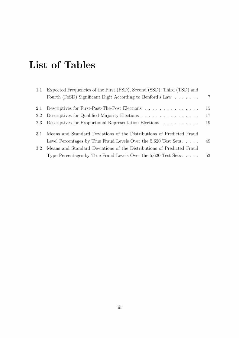
List of Tables
1.1 Expected Frequencies of the First (FSD), Second (SSD), Third (TSD) and
Fourth (FoSD) Significant Digit According to Benford’s Law . . . . . . . 7
2.1 Descriptives for First-Past-The-Post Elections . . . . . . . . . . . . . . . 15
2.2 Descriptives for Qualified Majority Elections . . . . . . . . . . . . . . . . 17
2.3 Descriptives for Proportional Representation Elections . . . . . . . . . . 19
3.1 Means and Standard Deviations of the Distributions of Predicted Fraud
Level Percentages by True Fraud Levels Over the 5,620 Test Sets . . . . . 49
3.2 Means and Standard Deviations of the Distributions of Predicted Fraud
Type Percentages by True Fraud Levels Over the 5,620 Test Sets . . . . . 53
iii
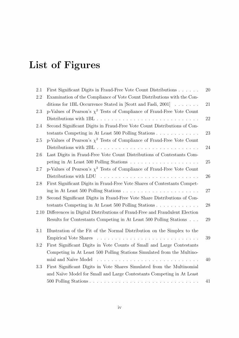
List of Figures
2.1 First Significant Digits in Fraud-Free Vote Count Distributions . . . . . . 20
2.2 Examination of the Compliance of Vote Count Distributions with the Con-
ditions for 1BL Occurrence Stated in [Scott and Fasli, 2001] . . . . . . . 21
2.3 p-Values of Pearson’s χ2 Tests of Compliance of Fraud-Free Vote Count
Distributions with 1BL . . . . . . . . . . . . . . . . . . . . . . . . . . . . 22
2.4 Second Significant Digits in Fraud-Free Vote Count Distributions of Con-
testants Competing in At Least 500 Polling Stations . . . . . . . . . . . . 23
2.5 p-Values of Pearson’s χ2 Tests of Compliance of Fraud-Free Vote Count
Distributions with 2BL . . . . . . . . . . . . . . . . . . . . . . . . . . . . 24
2.6 Last Digits in Fraud-Free Vote Count Distributions of Contestants Com-
peting in At Least 500 Polling Stations . . . . . . . . . . . . . . . . . . . 25
2.7 p-Values of Pearson’s χ2 Tests of Compliance of Fraud-Free Vote Count
Distributions with LDU . . . . . . . . . . . . . . . . . . . . . . . . . . . 26
2.8 First Significant Digits in Fraud-Free Vote Shares of Contestants Compet-
ing in At Least 500 Polling Stations . . . . . . . . . . . . . . . . . . . . . 27
2.9 Second Significant Digits in Fraud-Free Vote Share Distributions of Con-
testants Competing in At Least 500 Polling Stations . . . . . . . . . . . . 28
2.10 Differences in Digital Distributions of Fraud-Free and Fraudulent Election
Results for Contestants Competing in At Least 500 Polling Stations . . . 29
3.1 Illustration of the Fit of the Normal Distribution on the Simplex to the
Empirical Vote Shares . . . . . . . . . . . . . . . . . . . . . . . . . . . . 39
3.2 First Significant Digits in Vote Counts of Small and Large Contestants
Competing in At Least 500 Polling Stations Simulated from the Multino-
mial and Naıve Model . . . . . . . . . . . . . . . . . . . . . . . . . . . . 40
3.3 First Significant Digits in Vote Shares Simulated from the Multinomial
and Naıve Model for Small and Large Contestants Competing in At Least
500 Polling Stations . . . . . . . . . . . . . . . . . . . . . . . . . . . . . . 41
iv
3.4 Image Plots of ROC Curves from Test Set Evaluation of Binary Logistic
Regressions for Different Values of Fraud Parameters . . . . . . . . . . . 47
3.5 Image plots of ROC Curves from Test Set Evaluation of Binary Logistic
Regressions With Two Different Types of Fraud: Prevalent Ballot Stuffing
on the Left and Prevalent Vote Transferring on the Right . . . . . . . . . 48
3.6 Violin Plots of the Distributions of Predicted Fraud Levels Percentages by
True Fraud Levels Over the 5,620 Test Sets . . . . . . . . . . . . . . . . . 50
3.7 Comparison of Importance of the Five Digital Patterns for Classification
of Different Fraud Levels Using the Difference In Deviances . . . . . . . . 52
3.8 Violin Plots of the Distributions of Predicted Fraud Level Percentages by
True Fraud Types Over the 5,620 Test Sets . . . . . . . . . . . . . . . . . 54
3.9 Comparison of Importance of the Five Digital Patterns for Classification
of Different Fraud Types Using the Difference In Deviances . . . . . . . . 55
3.10 Second Significant Digits in Vote Counts for Small and Large Contestants
Competing in At Least 500 Polling Stations Simulated from the Multino-
mial and Naıve Model . . . . . . . . . . . . . . . . . . . . . . . . . . . . 70
3.11 Second Significant Digits in Vote Shares for Small and Large Contestants
Competing in At Least 500 Polling Stations Simulated from the Multino-
mial and Naıve Model . . . . . . . . . . . . . . . . . . . . . . . . . . . . 71
3.12 Last Digits in Vote Counts for Small and Large Contestants Competing in
At Least 500 Polling Stations Simulated from the Multinomial and Naıve
Model . . . . . . . . . . . . . . . . . . . . . . . . . . . . . . . . . . . . . 72
v
Introduction
“Electoral fraud is clearly the gravest form of electoral malpractice, and should be combated
overtly and publicly by all those with a stake in democratic development.”
[Lopez-Pintor, 2011, p. 3]
Without a doubt, elections constitute the very cornerstone of representative democ-
racy. Ensuring that a particular election is conducted democratically is, however, a
non-trivial task. The traditional approach, based on election observation [see Bjornlund,
2004, Hyde, 2008], has its limitations: observers monitor only a small number of polling
stations and their accounts can be questioned as partial. As Mebane writes, ‘election
monitoring is usually more focused on the conditions under which elections are con-
ducted – on whether they are free and fair – than whether they are accurate’ [Mebane,
2010c, p. 1; emphasis added].
In search of a better assessment of election accuracy, that is, the degree to which
official election results correspond to the true results, various methods of fraud detection
have been proposed. These are statistical techniques, attempting to identify patterns
in the large quantities of data produced in elections and use these patterns to distin-
guish between accurate and inaccurate electoral results. Although the techniques differ
substantially in their assumptions, they can all be considered tools of the emerging dis-
cipline called election forensics [Mebane, 2006]. Among the most widely applied as well
as controversial are methods of the so-called digital election forensics. Their proponents
claim that in fraud-free electoral data, distributions of digits at certain positions cor-
respond to theoretical distributions. Deviations from these theoretical distributions are
then considered to indicate electoral inaccuracies.
1

Given the high relevance of digital election forensics in the current academic and
non-academic debate, this dissertation will concentrate almost entirely on it; only the
literature review in the first chapter will briefly describe non-digital methods. From the
second chapter onwards, the applicability of different digital methods will be evaluated
using both empirical and simulated data. The second chapter will introduce the largest-
ever cross-national electoral dataset compiled at the polling-station level, collected almost
entirely by the author. The dataset will then be used to assess the occurrence of theo-
retical digital patterns in real-life elections. The third chapter will be simulation-based.
Many electoral contests will be simulated and electoral fraud will be artificially applied
to a subset. Logistic regression, using information on digital patterns, will be utilised to
separate the fraudulent and fraud-free electoral contests. The overall assessment will be
provided in the conclusion, together with an assessment of the limitations of the study
and implications for future research.
2

Chapter 1
Methods of Election Forensics
This chapter aims to provide an introduction to the context and methods of election
forensics. Throughout the whole chapter, the main driving question is: “How can we use
statistics to differentiate between fraud-free and fraudulent electoral data?”
The chapter starts with a section (1.1) introducing basic definitions that will be used
throughout the text. The second section (1.2) provides a short overview of general election
forensic techniques that have been used in the past. The following two sections then
concentrate on digital methods. Section 1.3 explores one of the most widely discussed
statistical ‘laws’, the so-called Benford’s law, which has constituted the main and the
most controversial digital forensic tool applied by election researchers. Section 1.4 is
dedicated to other digital methods.
3
1.1 Terminology
The following lists define core terms used in this dissertation. The first relates to the
organisation of elections:
Constituency An electoral unit in which seats are contested.
Election contest A competition for representation within a constituency.
Electoral contestant A political party, movement or candidate participating in an elec-tion contest.
Election A set of election contests from all constituencies.
Polling station An electoral unit on the level where votes are collected.
The second list is focused on electoral outcomes:
Vote counts The number of votes received by an electoral contestant in a polling station.
Vote shares Vote counts divided by their sum in a given polling station.
Election results Vote counts, vote shares and voter turnout.
Election-level results Election results for all polling stations in a given election.
Constituency-level results Election results for all polling stations by constituencies.
Size of vote count/share distribution The number of polling stations from whichelection results are available for a given contestant.
The remaining terms relate to fraud and election forensics:
Election inaccuracy Discrepancy between the official and true election results.
Election fraud Election inaccuracy caused by intentional manipulation of true electionresults. Unintentional errors are not considered fraud.
Ballot stuffing Fraud by filling ballot boxes with ballots for a specific contestant.
Vote transferring Fraud by transferring votes from a contestant to another contestant.
Digital forensics Statistical methods aimed at identifying election fraud by examina-tion of distributions of digits in election results.
Significant digit For any non-zero real number, first significant digit (FSD) is definedas its left-most non-zero digit. Second significant digit (SSD) is the digit to theright of the FSD. The FSD attains values from {1, 2, . . . , 9} and the SSD from{0, 1, . . . , 9}. Note that single-digit integers have no SSD.
Last digit For a non-negative integer, the last digit (LD) is defined as its right-mostdigit ({0, 1, . . . , 9}).
4
1.2 Non-Digital Election Forensics
This section briefly describes scholarship on general election forensics. It introduces
various ideas that have been used to detect electoral fraud.
The first line of reasoning compares election results in monitored and non-monitored
polling stations. Using the logic of field experiments, systematic differences in election
results between these polling stations are to be related to fraud [see Hanlon and Fox,
2006, Callen and Long, 2011, Enikolopov et al., 2012].
Another approach is to regress vote counts on relevant covariates and point to outliers
as being susceptible to fraud [see Wand et al., 2001a,b, Mebane and Sekhon, 2004]. This
method is designed to detect small-scale fraud occurring in a limited number of polling
stations. Large-scale systematic fraud is unlikely to be spotted by such a method.
Ecological regression has been employed to study the so-called flows of votes. Contes-
tants’ vote shares are regressed on their vote shares in a previous election. Homogeneity
of regression coefficients across all polling stations is assumed to avoid the ecological fal-
lacy. Their unusual values are used to make claims about the presence and magnitude of
fraud [see Myagkov et al., 2005, 2007, 2008, 2009, Park, 2008, Levin et al., 2009].
Based on the assumption that electoral fraud is in practice mostly implemented by
ballot stuffing, several studies have looked at the relationship between turnout and con-
testants’ vote shares using parametric or non-parametric regression [see Myagkov et al.,
2005, 2007, Vorobyev, 2011]. Most recently, Klimek et al. [2012] developed a parametric
model with parameters directly related to the number of fraudulent votes.
Unfortunately, the application of most non-digital methods to more than a few elec-
tions is problematic because specific information is required. Not always, for example, are
election monitors allowed to observe the election in randomly selected polling stations,
not always is fraud small-scale, and not always are previous election results for the same
contestants available. Because of these practical problems, it would be of great value
to have forensic methods which would require as little input as possible at our disposal.
With this in mind, I now move to the discussion of digital forensic methods.
5
1.3 Digital Forensics Using Benford’s Law
Digital forensics aims to validate electoral results based on election results only. It claims
that fraud-free data exhibit certain digital patterns and systematic deviations from these
patterns signal fraud. By far the most popular line of reasoning has been associated with
the so-called Benford’s law. This section starts with different explanations of why Ben-
ford’s law emerges in many empirical datasets. Next, its applications to fraud detection
are described, focusing on election forensics.
1.3.1 The Mathematics of Benford’s Law
In 1881, Simon Newcomb published a two-page note on the frequency of significant digits
in what he called ‘natural numbers’ [Newcomb, 1881]. After his observation that the first
pages of logarithmic tables are worn out much faster that the last ones, he followed his
intuition that numbers occurring in nature’ should be approached as ratios, and derived
the formulas for the expected frequencies of the first significant digit (FSD):
F (FSD = d) = log10
(d+ 1
d
), for d = 1, 2, . . . , 9,
and the second significant digit (SSD):
F (SSD = d) =9∑i=1
log10
(10i+ d+ 1
10i+ d
), for d = 0, 1, . . . , 9.
Newcomb also noted that the differences between expected frequencies of the third and
latter significant digits are minuscule; indeed the distribution of the j-th significant digit
approaches uniform distribution exponentially in j (Hill [1998]). Expected frequencies of
the first four significant digits are reported in Table 1.1. Newcomb’s findings remained
unnoticed for a long time, maybe due to the vagueness of the explanation (based on the
concept of ‘natural numbers’) he proposed for the phenomenon.
Almost 60 years later the law was rediscovered by Benford [1938] who published a
more rigorous analysis. He compiled 20 datasets with more than 20,000 observations in
total and showed that several of the datasets followed the law to a large degree. Benford
6

Table 1.1: Expected Frequencies of the First (FSD), Second (SSD), Third (TSD) andFourth (FoSD) Significant Digit According to Benford’s Law
Digit FSD SSD TSD FoSD
0 . 0.1197 0.1018 0.10021 0.3010 0.1139 0.1014 0.10012 0.1761 0.1088 0.1010 0.10013 0.1249 0.1043 0.1006 0.10014 0.0969 0.1003 0.1002 0.10005 0.0792 0.0967 0.0998 0.10006 0.0669 0.0934 0.0994 0.09997 0.0580 0.0904 0.0990 0.09998 0.0512 0.0876 0.0986 0.09999 0.0458 0.0850 0.0983 0.0998
Expected frequencies of first four significant digits using formulas from [Newcomb, 1881].
found the best fit when all 20 different datasets were merged into a single table.
Benford’s explanation of the phenomenon was very similar to that of Newcomb; he
believed that natural as well as human phenomena fall into a geometric series which
yields the observed digit patterns. He went as far as stating that “Nature counts
e0, ex, e2x, e3x, . . . and builds and functions accordingly.” [Benford, 1938, p. 563]
On this basis he formulated the ‘Law of Anomalous Numbers’, which is a generalisation
of Newcomb’s formulas for integers of limited length. Instead of ‘length’ he speaks of
‘orders’, with the order equal to one for numbers 1-10, two for 10-100, three for 100-1000
and so on. The Law of Anomalous Numbers for the FSDs states:
F r1 =
[log
10(2 · 10r−1 − 1)
10r − 1+
8
10r
]1
log 10,
F ra
a6=1
=
[log
(a+ 1)10r−1 − 1
a10r − 1+
1
10r
]1
log 10,
where a stands for all digits except 1 and r is the digital order.
Over the course of the 20th century, plenty of explanations for the wide occurrence of
Benford’s law in real-life datasets were proposed. In his comprehensive overview of the
then scholarship Raimi [1976] concluded that none of the pure mathematical explanations
(e.g. those based on number theory) proved satisfactory and urged for a statistical inter-
pretation of the law. He cited several statistical results describing satisfactory conditions
7
for statistical models under which Benford’s law emerges (see below).
Hill [1998] elaborated upon the idea that it may be the process of mixing different
distribution that leads to better compliance with Benford’s law. He introduced a proper
probabilistic framework and derived ‘the log-limit law for significant digits’. It states that
if we select probability distributions at random and then sample each of them in a way
that is scale neutral, then the digital distribution of the combined sample converges to
Benford’s law. Hence Hill explained Benford’s surprising result that the union of all his
tables fit the law best [also see Janvresse and de la Rue, 2004, Rodriguez, 2004].
Another line of statistical reasoning was associated with the notion of multiplicative
processes. Furry and Hurwitz [1945] looked at the logarithm of a product log Yn =
log Πni=1Xi =
∑ni=1 logXi of n independent and identically distributed random variables
Xi. Since under very weak conditions the central limit theorem applies to the latter sum,
then with increasing n the distribution of Yn approximates log-normal distribution. The
authors proved that log Yn(mod 1) approximates uniform distribution as n increases [also
see Adhikari and Sarkar, 1968, Adhikari, 1969, Boyle, 1994].
Which distributions satisfy Benford’s law? Scott and Fasli [2001] reported simulation
results showing that positively skewed non-zero unimodal distributions defined on a set
of positive numbers do follow it. The skew must be substantial with the mean at least
twice as high as the median. They found that the law is approximately followed by log-
normal distributions with the value of scale parameter no smaller than 1.2. Using signal
processing, Smith [1997] reached a similar conclusion, stating a good fit for distributions
wide in comparison to the unit distance on a logarithmic scale, e.g. wide log-normal
distributions.
Morrow [2010] proved that the compliance with Benford’s law improves as a random
variable is raised to higher powers. Looking at exponential-scale families of distribu-
tions closed under power transformations, sufficiently high values of scale parameter shall
therefore yield a good fit of log-normal distribution to Benford’s law. Results on other
distributions and distributional families can be found in [Leemis et al., 2000, Pietronero
et al., 2001, Engel and Leuenberger, 2003, Grendar et al., 2007].
8
1.3.2 Applications to Fraud Detection
The applicability of Benford’s law to a wide range of datasets gave rise to the idea of
using it to distinguish between manipulated and non-manipulated datasets. It has been
most popular for the examination of financial statements in financial fraud detection.
Busta and Sundheim [1992] used it to examine tax returns yet in 1992, but it was only
after the publication of Nigrini’s accounting-related PhD thesis [see Nigrini, 2000] that
digital forensics gained popularity. Different methods of separating fraudulent from fraud-
free data using Benford’s law have been used, ranging from simple tests [see Wallace,
2002] to neural networks [see Busta and Weinberg, 1998, Bhattacharya et al., 2011] and
unsupervised procedures [see Lu and Boritz, 2005, Lu et al., 2006].
One of the first applications of Benford’s law outside accounting is related to Carslaw’s
research on cognitive perceptions [see Carslaw, 1988]. Recently, Diekmann [2007] has
studied the digital distribution of unstandardised OLS regression coefficients published
in academic journals.
Following the wide use of Benford’s law in accounting and other fields, its variations
have also been applied in electoral research by examining digital distributions of vote
counts. Although the law was originally derived for continuous distributions, it could
well be applicable to discrete distributions. It has been hypothesised that fraud-free vote
counts are Benford-distributed, and if a deviation is found then it may be attributed to
election fraud. However, since polling stations are typically rather similar in size, the
first significant digit law should often not be expected. That is why the focus shifted
from testing Benford’s first digit law (1BL) to Benford’s second digit law (2BL). Mebane
has been the main proponent of this fraud detection strategy [see Mebane, 2006, 2007,
2008, Mebane and Kalinin, 2009, Mebane, 2011] but other authors have used it as well
[see Pericchi and Torres, 2011, Breunig and Goerres, 2011].
This approach has been criticised for the lack of a convincing theoretical explanation
as to why we should expect to observe 2BL in fraud-free electoral data [see Carter Center,
2005, Deckert et al., 2011]. Mebane [2010b] came up with two mechanisms that may lead
to data satisfying 2BL but not 1BL. The first one assumes that three types of voters
exist: those who favour the incumbent, those favouring opposition and those who make
9
their decisions at random. All polling stations are assumed to be of the same total
size and proportions of the voter types across polling stations vary according to uniform
distribution. Voters’ choices are, in this model, also subject to a small probability of
mistake.
The second mechanism features the same three types of voters. For each voter type,
the probabilities of voting for either of the two alternatives are the same in all polling
stations. Voter type proportions in each polling station vary according to normal distri-
butions. Polling station sizes are distributed uniformly. Relying on simulations, Mebane
[2010b] claimed that both the second and the first mechanism led to the distribution obey-
ing 2BL but not 1BL. Nevertheless, due to the specific nature of Mebane’s mechanisms,
their applicability to real-life elections remains questionable.
The overall lack of support for the occurrence of Benford’s law in electoral results did
not stop political scientists from assuming it. Several studies [see Mebane, 2010a,b, Cantu
and Saiegh, 2011] simulated electoral results based on the assumption that Benford’s law
holds (either 1BL or 2BL). The most sophisticated of the simulation analyses is the one
by Cantu and Saiegh [2011]. They artificially introduced fraud to the simulated data by a
simple mechanism of moving a proportion of one contestants’ votes to another contestant
and adding some extra ballot-stuffed votes. They proceeded to train a supervised machine
learning classifier (naıve Bayes) to distinguish between the fraudulent and fraud-free
simulated electoral contests; independent variables having been related to vote count
digital distributions.
In order to tackle the low validity of the Benford’s law assumption, Cantu and Saiegh
[2011] calibrated the synthetic data with real-world electoral data. Their ad hoc cali-
bration, however, does not help to answer the question of the applicability of Benford’s
law to fraud-free electoral data in general. This dissertation aims to improve on their
methodology by both assessing the validity of the Benford’s law assumption on a large
empirical dataset and using empirical data for synthetic data generation.
10
1.4 Other Digital Election Forensics Methods
It can be shown that under weak theoretical conditions, last digits of large-enough vote
counts are expected to occur with equal frequency. Proofs for certain continuous distri-
butions were provided by [Mosimann and Ratnaparkhi, 1996, Dlugosz and Muller-Funk,
2009] but these are not well-suited for inherently discrete electoral returns. Beber and
Scacco [2012] extended the previous work and used simulations to illustrate the behaviour
of several distributions. These showed that uniformity cannot be expected [Beber and
Scacco, 2012, p. 5]:
1. If a distribution has a standard deviation too small (about less than 10) because
draws from such distributions cluster within a very narrow range of numbers.
2. If a distribution has a fixed upper bound and draws that cluster at this bound.
However, even minor variations in polling station size (in tens of votes) will restore
last digit uniformity.
3. If a distribution has a mean relatively small compared to its standard deviation
because such a distribution generates a large number of very small counts.
When the numbers on electoral sheets are artificially modified by electoral commis-
sioners to favour a given party, they are likely to deviate from uniformity. The reason is
that people are rather bad at generating random numbers and so they introduce biases
into the data [see Mosimann et al., 1995]. The focus on the last digits of a sufficiently long
number is equivalent to focusing on inconsequential noise. This approach complements
the focus on ballot-stuffing which is typical for significant-digit analysis.
Apart from last-digit uniformity (LDU), Beber and Scacco [2012] discussed other
digital patterns that humans (even with incentives to randomise) tend to introduce into
data. For example, based on some experimental research they claimed that humans select
lower digits more often then higher digits, they avoid repetitions of digits and that they
tend to select pairs of distant numbers infrequently. While these constitute interesting
hypotheses, the focus of this dissertation will remain on the validity of 1BL, 2BL and
LDU for fraud-free election data as these are the three main open questions in the current
election fraud discussion.
11
Chapter 2
Empirical Data Analysis
It is striking how little empirical evaluation of the validity of digital election forensics
assumptions has been performed. Despite having direct political implications and thus
high social relevance, empirical studies applying Benford’s law to fraud detection have
either assumed the law’s validity or tried to ‘support’ it by illustrating its fit in one or
two elections only. Mebane [2006] looked at two elections (from the U.S. and Mexico),
Mebane [2007] at a single Mexican election, Mebane [2008] at one U.S. election, Mebane
and Kalinin [2009] at four Russian elections, Breunig and Goerres [2011] at five German
elections and Pericchi and Torres [2011] at 5 elections and a referendum from 3 countries.
Clearly, no compelling evidence has yet been used to support the use of Benford’s law.
On the other hand, critics of the applicability of Benford’s law to election results have
not provided comprehensive empirical evidence either. The Carter Center [2005] cited an
analysis showing a bad fit 2BL in a single election, and the most influential 2BL critique
by Deckert et al. [2011] only analysed two elections at the polling-station level. Any
analysis of electoral returns from a handful of elections can hardly provide satisfactory
evidence to reject the existence of Benford-like patterns in election results.
The hypothesis of last-digit uniformity has also not been thoroughly empirically stud-
ied; only a single article has been published on the topic in the election context. Since
the article demonstrates the phenomenon in only 4 elections, more empirical validation
is needed.
Having said all of the above, the natural next step would be to evaluate the digital
patterns on a substantial number of real-life elections. Large amounts of low-level cross-
12

national electoral data have been collected by the author for this purpose. To the best
of my knowledge, not only have cross-national polling-station data never been used to
a comparable extent in election forensics, they have not even been comparably used in
political science generally.
This chapter continues with a brief description of the dataset. The focus then shifts
to an evaluation of 1BL, 2BL and LDU on the dataset.
13
2.1 Description of the Dataset
To assess the validity of Benford’s law validity, online availability of election results (at
the polling-station level, as defined in Section 1.1) was checked for all countries in the
world. The process of data collection, data cleaning and data manipulation was very
time-consuming and tedious as the format and quality of posted election results varies
greatly from country to country. The final dataset contains vote counts from 24 coun-
tries gathered either from primary online sources (typically national election commission
websites) or from reliable secondary sources (data used in peer-reviewed journal articles).
It is essential to determine the appropriate level of analysis. First, polling-station
electoral data must be analysed, as stressed by Mebane [2011]. Polling stations constitute
the level at which manipulation with ballot boxes occurs, and no further information is
lost as compared to working with more aggregated data.
Second, elections are organised in constituencies with separate election contests. Since
voters in different constituencies vote for different contestants, it is often not sensible
to combine election results across constituencies. Even if cross-constituency election
results could be sensibly combined, for example by looking at political parties rather
than individual candidates in British general elections, their distributions are likely to
be substantially different and merging them could result in mixtures that are hard to
analyse. For example, a regional party may be very successful in a few constituencies
only and not even run candidates in other constituencies. This is why the primary focus
of this dissertation rests on election contests as opposed to elections.
In order to make the dataset description as clear as possible, this section will be
organised according to the type of electoral system at use in a given election. The
importance of constituencies in this analysis requires an understanding of how they differ
across electoral systems. It has also been established that different electoral rules induce
different types of strategic behaviour of voters [see Duverger, 1959, Cox, 1997] and the
effect of election rules on digital distributions has been analysed by Mebane [2010a,b].
The three most widely employed electoral systems in the world are: first-past-the-post
(FPTP), qualified majority (QM) and proportional representation (PR). FPTP is applied
in single-seat constituencies with each voter casting a single vote and with the candidate
14
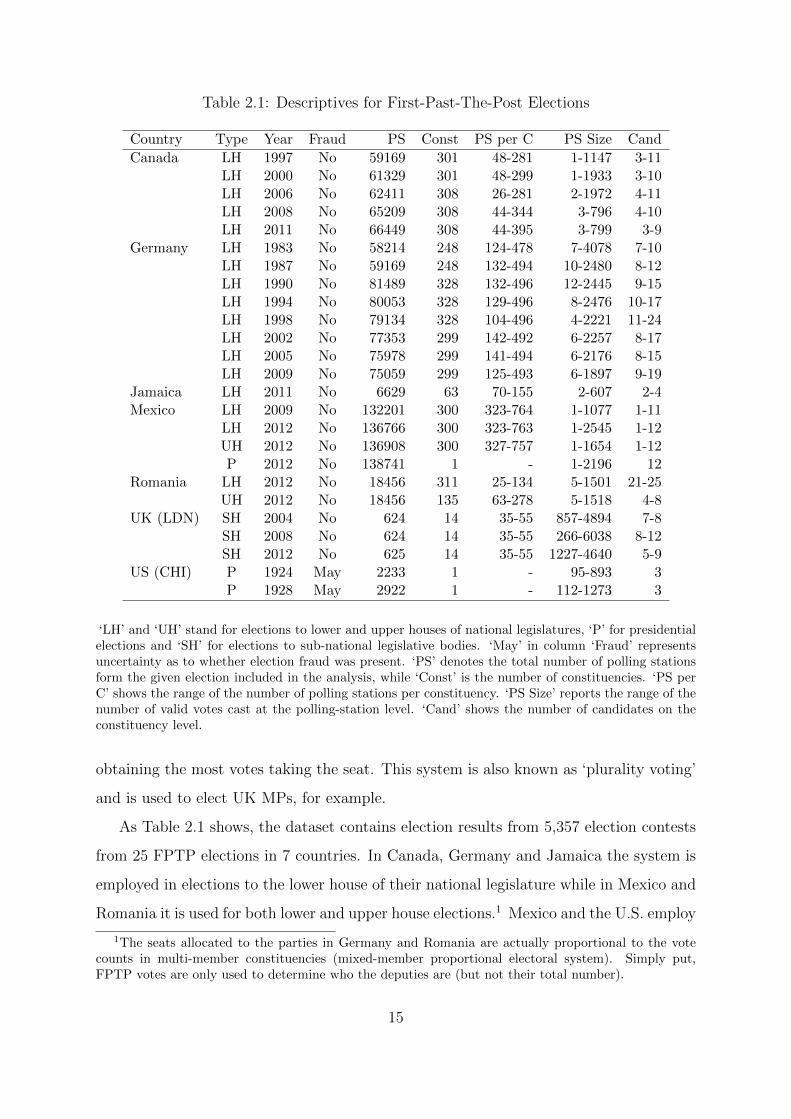
Table 2.1: Descriptives for First-Past-The-Post Elections
Country Type Year Fraud PS Const PS per C PS Size Cand
Canada LH 1997 No 59169 301 48-281 1-1147 3-11LH 2000 No 61329 301 48-299 1-1933 3-10LH 2006 No 62411 308 26-281 2-1972 4-11LH 2008 No 65209 308 44-344 3-796 4-10LH 2011 No 66449 308 44-395 3-799 3-9
Germany LH 1983 No 58214 248 124-478 7-4078 7-10LH 1987 No 59169 248 132-494 10-2480 8-12LH 1990 No 81489 328 132-496 12-2445 9-15LH 1994 No 80053 328 129-496 8-2476 10-17LH 1998 No 79134 328 104-496 4-2221 11-24LH 2002 No 77353 299 142-492 6-2257 8-17LH 2005 No 75978 299 141-494 6-2176 8-15LH 2009 No 75059 299 125-493 6-1897 9-19
Jamaica LH 2011 No 6629 63 70-155 2-607 2-4Mexico LH 2009 No 132201 300 323-764 1-1077 1-11
LH 2012 No 136766 300 323-763 1-2545 1-12UH 2012 No 136908 300 327-757 1-1654 1-12P 2012 No 138741 1 - 1-2196 12
Romania LH 2012 No 18456 311 25-134 5-1501 21-25UH 2012 No 18456 135 63-278 5-1518 4-8
UK (LDN) SH 2004 No 624 14 35-55 857-4894 7-8SH 2008 No 624 14 35-55 266-6038 8-12SH 2012 No 625 14 35-55 1227-4640 5-9
US (CHI) P 1924 May 2233 1 - 95-893 3P 1928 May 2922 1 - 112-1273 3
‘LH’ and ‘UH’ stand for elections to lower and upper houses of national legislatures, ‘P’ for presidentialelections and ‘SH’ for elections to sub-national legislative bodies. ‘May’ in column ‘Fraud’ representsuncertainty as to whether election fraud was present. ‘PS’ denotes the total number of polling stationsform the given election included in the analysis, while ‘Const’ is the number of constituencies. ‘PS perC’ shows the range of the number of polling stations per constituency. ‘PS Size’ reports the range of thenumber of valid votes cast at the polling-station level. ‘Cand’ shows the number of candidates on theconstituency level.
obtaining the most votes taking the seat. This system is also known as ‘plurality voting’
and is used to elect UK MPs, for example.
As Table 2.1 shows, the dataset contains election results from 5,357 election contests
from 25 FPTP elections in 7 countries. In Canada, Germany and Jamaica the system is
employed in elections to the lower house of their national legislature while in Mexico and
Romania it is used for both lower and upper house elections.1 Mexico and the U.S. employ
1The seats allocated to the parties in Germany and Romania are actually proportional to the votecounts in multi-member constituencies (mixed-member proportional electoral system). Simply put,FPTP votes are only used to determine who the deputies are (but not their total number).
15
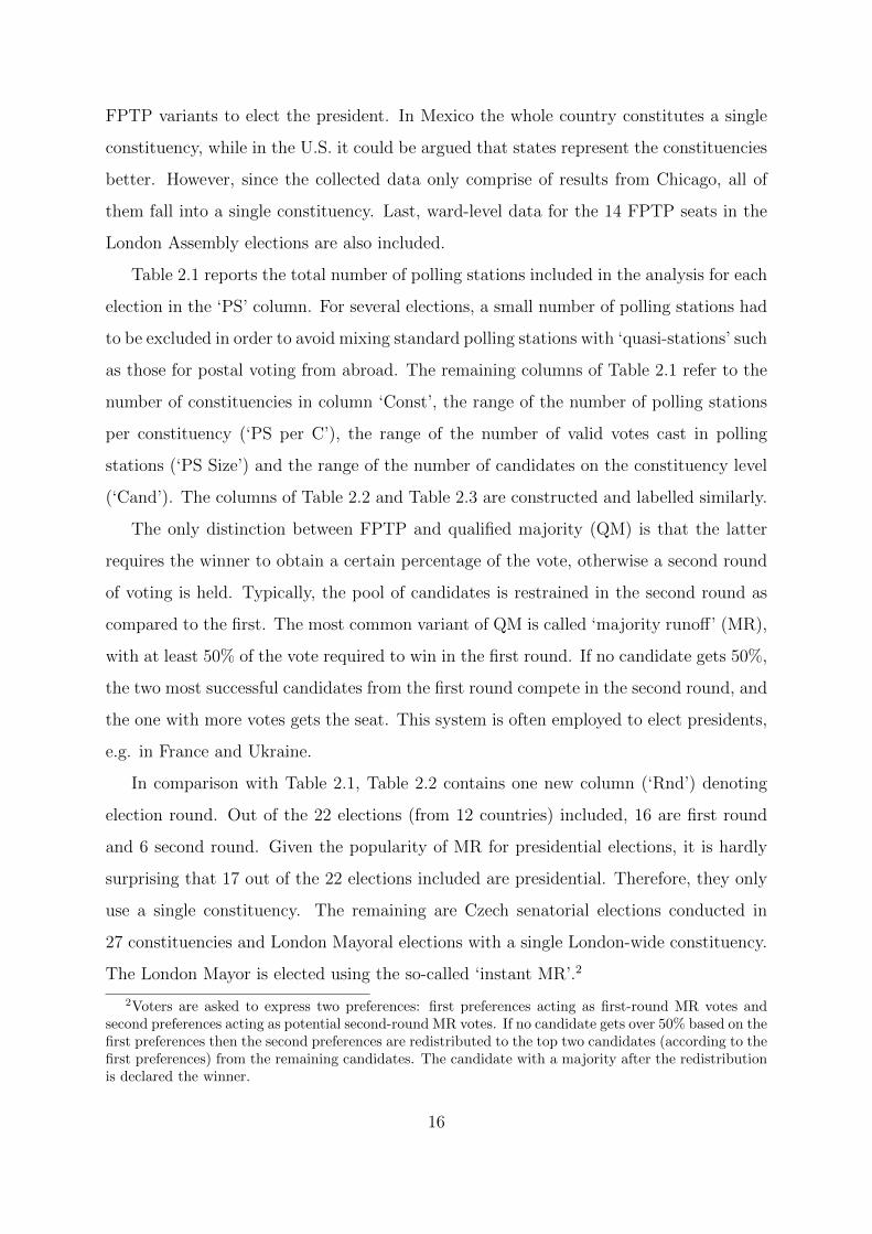
FPTP variants to elect the president. In Mexico the whole country constitutes a single
constituency, while in the U.S. it could be argued that states represent the constituencies
better. However, since the collected data only comprise of results from Chicago, all of
them fall into a single constituency. Last, ward-level data for the 14 FPTP seats in the
London Assembly elections are also included.
Table 2.1 reports the total number of polling stations included in the analysis for each
election in the ‘PS’ column. For several elections, a small number of polling stations had
to be excluded in order to avoid mixing standard polling stations with ‘quasi-stations’ such
as those for postal voting from abroad. The remaining columns of Table 2.1 refer to the
number of constituencies in column ‘Const’, the range of the number of polling stations
per constituency (‘PS per C’), the range of the number of valid votes cast in polling
stations (‘PS Size’) and the range of the number of candidates on the constituency level
(‘Cand’). The columns of Table 2.2 and Table 2.3 are constructed and labelled similarly.
The only distinction between FPTP and qualified majority (QM) is that the latter
requires the winner to obtain a certain percentage of the vote, otherwise a second round
of voting is held. Typically, the pool of candidates is restrained in the second round as
compared to the first. The most common variant of QM is called ‘majority runoff’ (MR),
with at least 50% of the vote required to win in the first round. If no candidate gets 50%,
the two most successful candidates from the first round compete in the second round, and
the one with more votes gets the seat. This system is often employed to elect presidents,
e.g. in France and Ukraine.
In comparison with Table 2.1, Table 2.2 contains one new column (‘Rnd’) denoting
election round. Out of the 22 elections (from 12 countries) included, 16 are first round
and 6 second round. Given the popularity of MR for presidential elections, it is hardly
surprising that 17 out of the 22 elections included are presidential. Therefore, they only
use a single constituency. The remaining are Czech senatorial elections conducted in
27 constituencies and London Mayoral elections with a single London-wide constituency.
The London Mayor is elected using the so-called ‘instant MR’.2
2Voters are asked to express two preferences: first preferences acting as first-round MR votes andsecond preferences acting as potential second-round MR votes. If no candidate gets over 50% based on thefirst preferences then the second preferences are redistributed to the top two candidates (according to thefirst preferences) from the remaining candidates. The candidate with a majority after the redistributionis declared the winner.
16
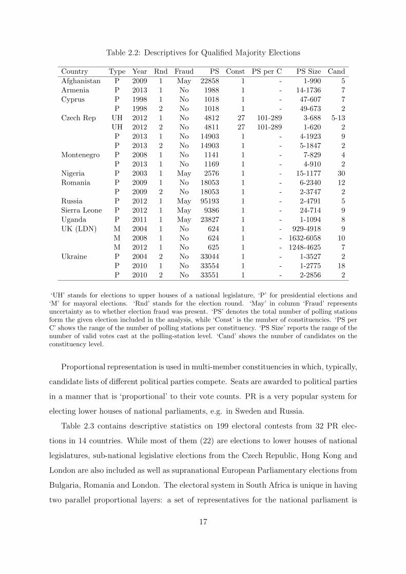
Table 2.2: Descriptives for Qualified Majority Elections
Country Type Year Rnd Fraud PS Const PS per C PS Size Cand
Afghanistan P 2009 1 May 22858 1 - 1-990 5Armenia P 2013 1 No 1988 1 - 14-1736 7Cyprus P 1998 1 No 1018 1 - 47-607 7
P 1998 2 No 1018 1 - 49-673 2Czech Rep UH 2012 1 No 4812 27 101-289 3-688 5-13
UH 2012 2 No 4811 27 101-289 1-620 2P 2013 1 No 14903 1 - 4-1923 9P 2013 2 No 14903 1 - 5-1847 2
Montenegro P 2008 1 No 1141 1 - 7-829 4P 2013 1 No 1169 1 - 4-910 2
Nigeria P 2003 1 May 2576 1 - 15-1177 30Romania P 2009 1 No 18053 1 - 6-2340 12
P 2009 2 No 18053 1 - 2-3747 2Russia P 2012 1 May 95193 1 - 2-4791 5Sierra Leone P 2012 1 May 9386 1 - 24-714 9Uganda P 2011 1 May 23827 1 - 1-1094 8UK (LDN) M 2004 1 No 624 1 - 929-4918 9
M 2008 1 No 624 1 - 1632-6058 10M 2012 1 No 625 1 - 1248-4625 7
Ukraine P 2004 2 No 33044 1 - 1-3527 2P 2010 1 No 33554 1 - 1-2775 18P 2010 2 No 33551 1 - 2-2856 2
‘UH’ stands for elections to upper houses of a national legislature, ‘P’ for presidential elections and‘M’ for mayoral elections. ‘Rnd’ stands for the election round. ‘May’ in column ‘Fraud’ representsuncertainty as to whether election fraud was present. ‘PS’ denotes the total number of polling stationsform the given election included in the analysis, while ‘Const’ is the number of constituencies. ‘PS perC’ shows the range of the number of polling stations per constituency. ‘PS Size’ reports the range of thenumber of valid votes cast at the polling-station level. ‘Cand’ shows the number of candidates on theconstituency level.
Proportional representation is used in multi-member constituencies in which, typically,
candidate lists of different political parties compete. Seats are awarded to political parties
in a manner that is ‘proportional’ to their vote counts. PR is a very popular system for
electing lower houses of national parliaments, e.g. in Sweden and Russia.
Table 2.3 contains descriptive statistics on 199 electoral contests from 32 PR elec-
tions in 14 countries. While most of them (22) are elections to lower houses of national
legislatures, sub-national legislative elections from the Czech Republic, Hong Kong and
London are also included as well as supranational European Parliamentary elections from
Bulgaria, Romania and London. The electoral system in South Africa is unique in having
two parallel proportional layers: a set of representatives for the national parliament is
17
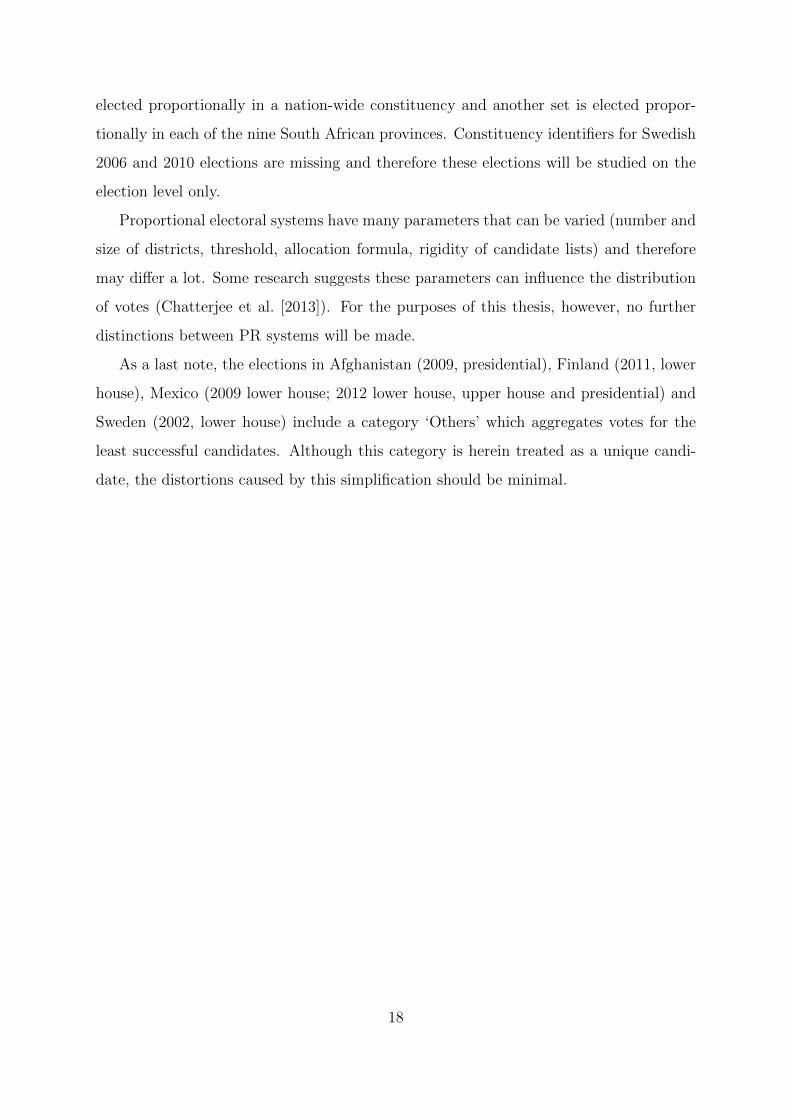
elected proportionally in a nation-wide constituency and another set is elected propor-
tionally in each of the nine South African provinces. Constituency identifiers for Swedish
2006 and 2010 elections are missing and therefore these elections will be studied on the
election level only.
Proportional electoral systems have many parameters that can be varied (number and
size of districts, threshold, allocation formula, rigidity of candidate lists) and therefore
may differ a lot. Some research suggests these parameters can influence the distribution
of votes (Chatterjee et al. [2013]). For the purposes of this thesis, however, no further
distinctions between PR systems will be made.
As a last note, the elections in Afghanistan (2009, presidential), Finland (2011, lower
house), Mexico (2009 lower house; 2012 lower house, upper house and presidential) and
Sweden (2002, lower house) include a category ‘Others’ which aggregates votes for the
least successful candidates. Although this category is herein treated as a unique candi-
date, the distortions caused by this simplification should be minimal.
18
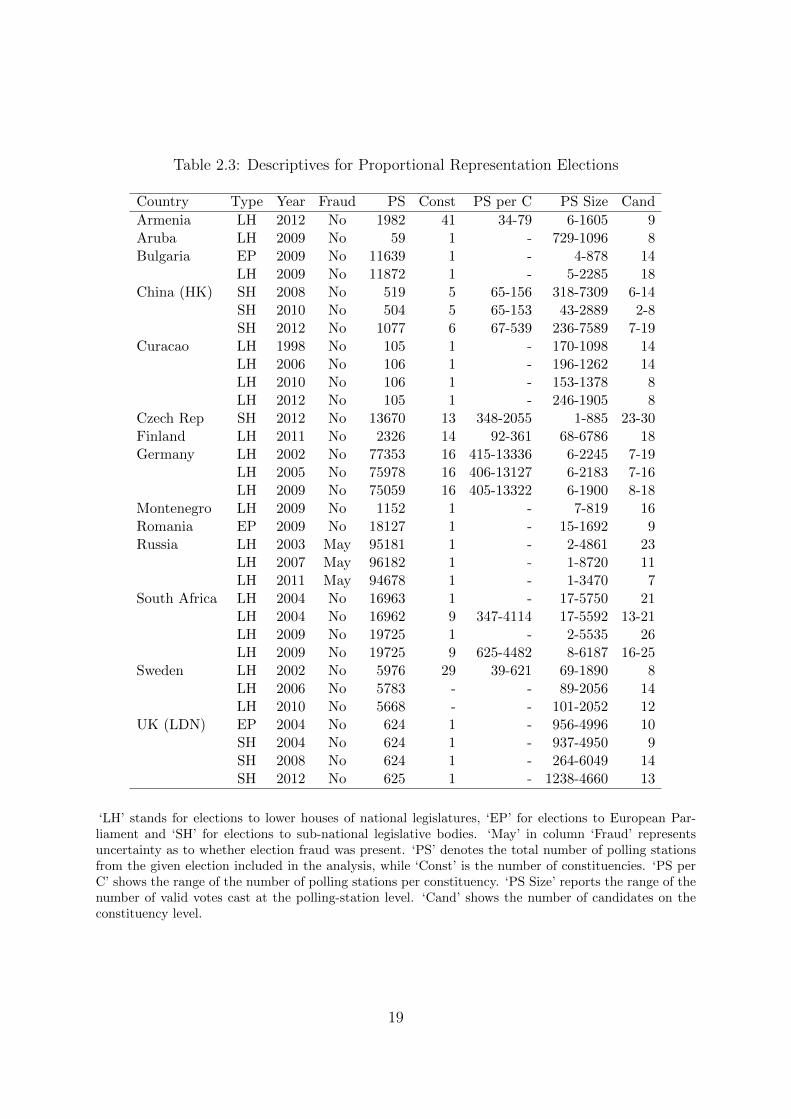
Table 2.3: Descriptives for Proportional Representation Elections
Country Type Year Fraud PS Const PS per C PS Size Cand
Armenia LH 2012 No 1982 41 34-79 6-1605 9Aruba LH 2009 No 59 1 - 729-1096 8Bulgaria EP 2009 No 11639 1 - 4-878 14
LH 2009 No 11872 1 - 5-2285 18China (HK) SH 2008 No 519 5 65-156 318-7309 6-14
SH 2010 No 504 5 65-153 43-2889 2-8SH 2012 No 1077 6 67-539 236-7589 7-19
Curacao LH 1998 No 105 1 - 170-1098 14LH 2006 No 106 1 - 196-1262 14LH 2010 No 106 1 - 153-1378 8LH 2012 No 105 1 - 246-1905 8
Czech Rep SH 2012 No 13670 13 348-2055 1-885 23-30Finland LH 2011 No 2326 14 92-361 68-6786 18Germany LH 2002 No 77353 16 415-13336 6-2245 7-19
LH 2005 No 75978 16 406-13127 6-2183 7-16LH 2009 No 75059 16 405-13322 6-1900 8-18
Montenegro LH 2009 No 1152 1 - 7-819 16Romania EP 2009 No 18127 1 - 15-1692 9Russia LH 2003 May 95181 1 - 2-4861 23
LH 2007 May 96182 1 - 1-8720 11LH 2011 May 94678 1 - 1-3470 7
South Africa LH 2004 No 16963 1 - 17-5750 21LH 2004 No 16962 9 347-4114 17-5592 13-21LH 2009 No 19725 1 - 2-5535 26LH 2009 No 19725 9 625-4482 8-6187 16-25
Sweden LH 2002 No 5976 29 39-621 69-1890 8LH 2006 No 5783 - - 89-2056 14LH 2010 No 5668 - - 101-2052 12
UK (LDN) EP 2004 No 624 1 - 956-4996 10SH 2004 No 624 1 - 937-4950 9SH 2008 No 624 1 - 264-6049 14SH 2012 No 625 1 - 1238-4660 13
‘LH’ stands for elections to lower houses of national legislatures, ‘EP’ for elections to European Par-liament and ‘SH’ for elections to sub-national legislative bodies. ‘May’ in column ‘Fraud’ representsuncertainty as to whether election fraud was present. ‘PS’ denotes the total number of polling stationsfrom the given election included in the analysis, while ‘Const’ is the number of constituencies. ‘PS perC’ shows the range of the number of polling stations per constituency. ‘PS Size’ reports the range of thenumber of valid votes cast at the polling-station level. ‘Cand’ shows the number of candidates on theconstituency level.
19
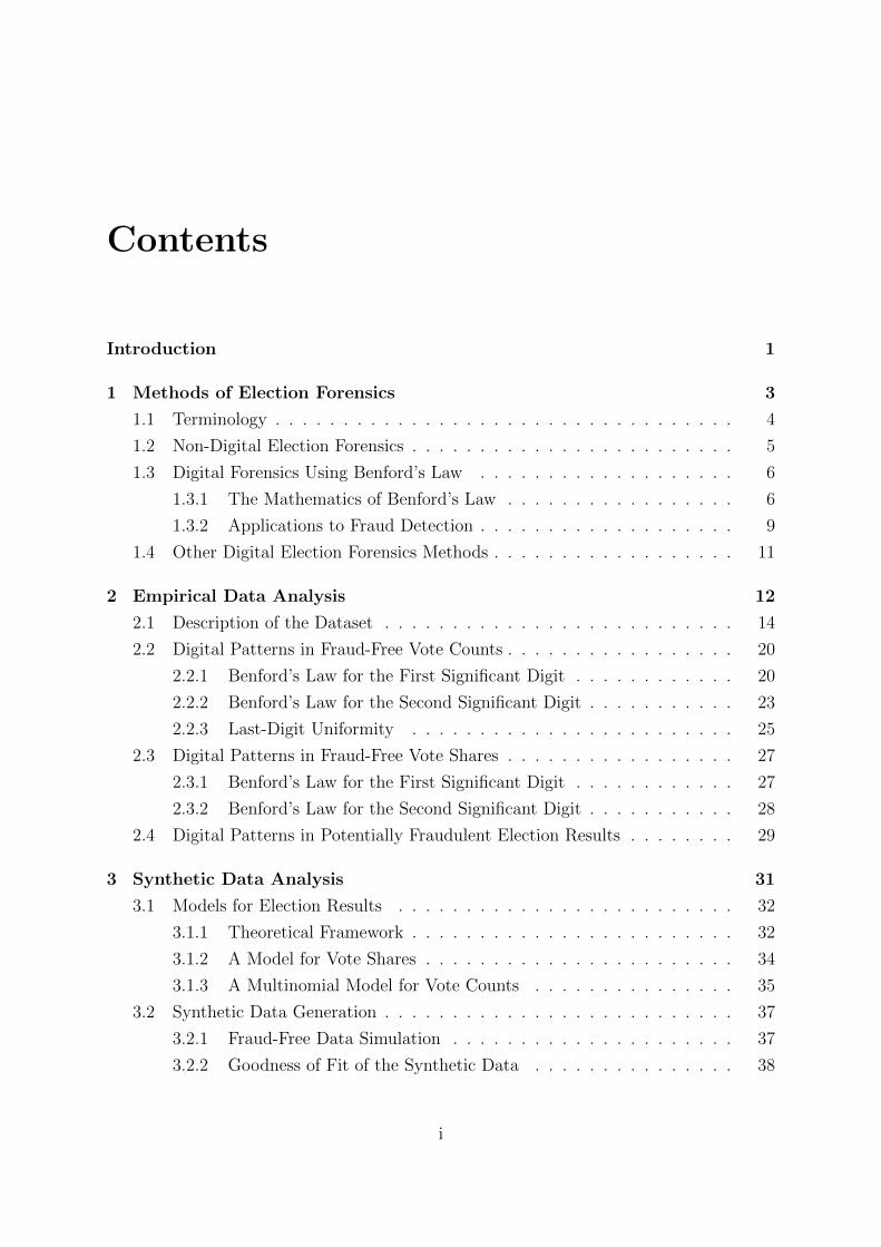
2.2 Digital Patterns in Fraud-Free Vote Counts
This section looks at whether 1BL, 2BL and LDU hold for empirical vote counts in 69
fraud-free elections. Fraud-free vote shares are analysed in Section 2.3 and election results
from 10 potentially fraudulent elections area analysed in Section 2.4. Constituency-level
vote count and vote share distributions constitute the units of analysis in all three sections.
Both visualization and statistical testing are used to assess their digital distributional fit.
2.2.1 Benford’s Law for the First Significant Digit
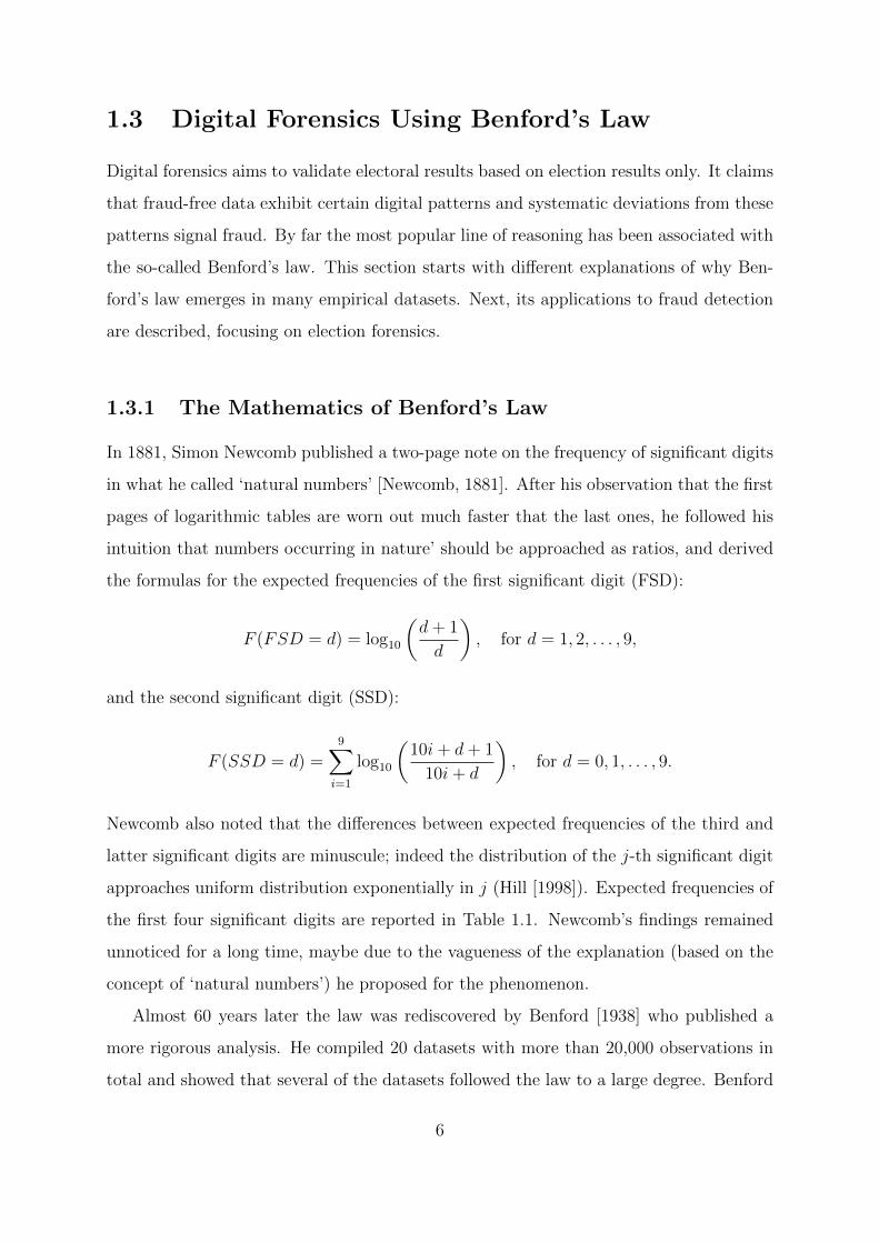
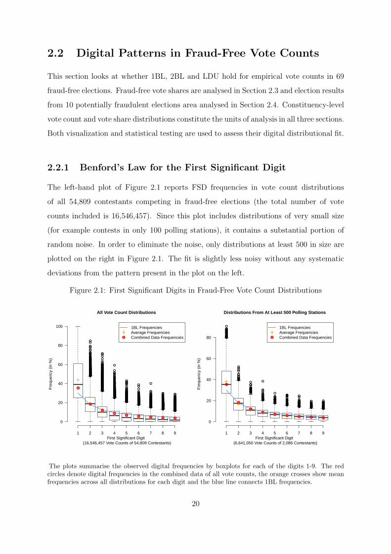
The left-hand plot of Figure 2.1 reports FSD frequencies in vote count distributions
of all 54,809 contestants competing in fraud-free elections (the total number of vote
counts included is 16,546,457). Since this plot includes distributions of very small size
(for example contests in only 100 polling stations), it contains a substantial portion of
random noise. In order to eliminate the noise, only distributions at least 500 in size are
plotted on the right in Figure 2.1. The fit is slightly less noisy without any systematic
deviations from the pattern present in the plot on the left.
Figure 2.1: First Significant Digits in Fraud-Free Vote Count Distributions
●
●
●●
●
●
●●●●
●
●
●●●●
●
●●
●
●
●
●
●
●
●●●●●●
●●●●
●●
●
●
●
●●●●●
●
●
●●●●●●●
●
●
●
●●
●●
●
●●●●
●
●●●●●
●
●
●
●●●●●
●●●
●
●
●
●
●
●
●●●●
●
●
●●
●
●
●
●●●●
●
●●●●●●●
●●
●●
●
●
●
●●
●
●●
●●
●●●
●
●
●●
●
●
●
●
●●●
●●●
●
●
●●
●
●
●
●
●
●
●●
●●
●
●●●●
●●
●●
●
●
●
●
●
●
●●●
●
●
●
●
●
●
●
●●●
●
●
●●●
●●
●●●●●●●
●
●●●●●
●●
●●
●●●●
●
●
●
●
●●●●
●●
●
●
●
●
●●
●●
●●
●●
●
●●
●
●
●
●
●●
●
●
●
●
●
●●
●
●
●
●
●
●●
●
●●●
●●
●
●●●
●
●
●
●●
●●
●
●
●●
●
●
●●●●
●
●
●●●●
●●●●●●
●
●●●●
●
●●
●
●
●
●
●
●
●
●
●
●
●
●
●●
●●●●
●
●●
●●●
●
●
●●
●●●●
●
●●●
●●●●●●
●
●
●●
●●●●●
●
●
●
●
●
●
●
●
●
●
●
●
●
●●
●
●●●●●
●
●
●
●
●
●
●
●
●●
●
●
●●●●●
●●
●
●●
●
●
●
●●
●
●
●
●●
●●●
●●●●●●●●
●
●●
●●●
●●
●●●●●●
●
●●●
●
●●
●
●●●●●●●●●●●
●
●●●●
●●●
●
●●●
●●
●
●
●
●
●●●
●●●
●●●●●
●
●
●●●
●
●
●●●
●
●●●
●
●●●●●
●
●●
●
●●●●
●
●●●●●
●
●●●●●●●●●●●
●
●●●●●●
●
●
●●
●
●●
●
●●
●
●
●
●
●●
●
●
●●
●●●●
●●
●●
●
●●
●
●
●
●
●
●●●
●
●●●●
●
●
●
●●●●
●●
●
●●●●●●●●●●●●●●●●
●●●●
●
●●
●
●●●●●●●●●●●●●●●●●●
●
●
●
●●
●
●
●
●
●
●●
●●
●●
●
●
●
●●
●
●●
●
●●●
●●
●
●●●
●
●
●●●
●
●●●
●
●
●●●
●
●
●●●
●●●●●
●
●
●●●●
●
●
●●
●
●●●
●
●
●
●●●
●●
●●●●
●
●●●●
●
●
●
●●●●●●●●●●●●
●
●
●
●●
●●●
●
●●
●
●
●
●
●●●
●●●
●
●
●
●
●●●
●●●●●
●
●
●●●
●●●
●●
●
●
●
●●
●●●●●●
●
●
●
●●
●●●
●●●●
●
●●●●●
●●●●
●
●●
●
●●●
●
●
●
●
●●
●●●●
●
●
●
●
●●
●
●
●
●●●
●●
●●
●
●
●
●
●
●●
●
●
●
●
●
●●
●●●
●
●●●●●
●
●
●
●
●●
●
●
●●
●
●●
●
●●●●●●●●●●●
●●●
●
●
●●●●●●●●●
●●
●●
●
●●●●●
●
●●
●●
●
●
●
●
●
●
●
●●
●
●●
●
●
●
●
●●
●
●
●
●●●
●●
●
●
●●
●
●●●●
●
●●
●
●
●
●●●●●
●●●●
●●●●
●
●●●●
●
●●
●●
●
●
●
●●●
●
●●●
●
●●
●●
●
●
●
●●●
●●
●
●
●
●
●
●●
●●●●●
●
●●●●●
●
●●●●●
●●
●●
●
●
●●
●
●●
●
●●●
●
●
●●●●●
●●
●
●●
●
●●●
●
●
●
●●
●●●
●●●
●●
●●●
●●
●●
●●
●
●
●
●
●●●
●
●
●●
●
●
●●
●
●●
●
●
●
●●
●●●●
●●
●●●●
●●●●●●
●
●
●●
●
●
●●●
●
●
●
●
●
●
●
●
●●
●●
●
●
●●●
●●
●●
●
●●
●●
●
●
●
●
●
●
●
●●●●●
●
●
●●●●
●●
●
●●●
●
●
●
●
●
●
●
●
●●
●●
●
●
●
●
●
●
●●●
●
●
●
●●
●
●
●
●
●
●
●
●
●
●
●
●
●
●●
●●●●●
●
●
●●●
●
●●
●●
●●●
●●
●
●
●
●
●
●
●
●
●
●
●
●
●●●
●
●
●
●●
●●●
●●
●●●●
●
●●
●
●
●●
●
●
●●●●
●●
●
●
●●
●
●●●
●●●●●
●●
●●●●●
●
●
●●●●●
●
●●●●●●
●
●●●●●●●●●●●●●●
●●●
●
●●●●
●
●●●●●●●●●
●
●●●●●●●●●
●●●●●●●●●●
●●●●
●●●●●●●●●●●●●●●
●
●●●
●
●
●●●●●●
●
●
●●●●●
●
●
●
●
●●●
●
●
●
●●
●
●
●
●
●●
●
●
●
●●●●●●●●●●●●●●●●
●●●
●
●●●
●●●
●
●●
●
●
●●
●
●●
●●●●●●
●●
●●●●●●
●
●
●●●
●
●
●
●●
●●
●
●●●●●
●
●●
●
●
●
●●●
●
●●●
●
●
●●●
●
●
●
●
●
●
●
●
●
●●
●●
●●●●●●●●
●●●
●
●
●
●
●
●
●
●●
●●
●●
●●●●●●
●
●●●●●
●
●
●●
●
●●●●●
●
●
●
●●
●
●●
●
●
●●
●
●●●●
●●●●●●●
●●●●●
●
●●●●●●
●
●●●
●
●●●●●●●
●●●●●●●●●●
●●●●
●
●
●●●
●●●●●
●●●●●
●
●●
●●
●
●
●
●
●
●●●●
●
●
●●●
●●●●●
●●●●●
●●
●
●
●
●●
●●●
●
●●●●●●●●
●●●
●●●●●
●
●●●●●
●●●●●●
●
●●
●●
●●●●
●
●
●
●
●●
●
●
●●●
●
●●●●●●●●
●●
●
●●●●●●●●●●
●
●●●●●●●
●●●●
●●
●
●●
●●●●
●
●
●●●
●●●●
●
●●
●
●
●●●●
●●●
●
●
●
●
●
●●●
●●●
●
●
●●
●●●
●
●
●
●●●
●
●
●
●●
●
●
●
●●●
●
●
●●●
●●
●
●●
●
●●
●
●
●●●●
●
●
●●
●
●●
●●
●●●●
●●●
●
●●●
●
●●
●●
●●
●
●
●●●●
●●●●●
●
●●●
●●●●●●●●●●
●
●●
●
●●●●
●
●
●●
●●
●●●●●●●●
●
●
●●●●
●
●●●●●●●
●
●●●●●●●●●●●●●●
●●●●●●●●●●●●●
●
●●●●
●●
●
●
●
●●
●●●●●●●●●●●●●●●●
●
●●●●
●●
●●●●●
●
●
●●●
●
●●●●●●●●●
●●●
●
●●●●
●●●●●
●
●●●●●●●●●
●●
●●●●●
●●●
●●●●●●●●●●
●●
●
●
●●●●
●●
●
●
●
●
●●●●
●
●●●
●●●●
●
●●
●●●●●●●
●
●●●
●●
●●
●●
●●●●
●
●
●
●●●●●
●
●●●
●●●●●●●●
●●●●●●●●●●●●
●
●
●
●●●●●●●
●●●●●
●
●●●●
●●●●●●
●
●●
●●●
●
●
●●
●
●
●
●●●●●
●
●●●●●●●●●●●●●●
●
●●●●●
●
●●
●
●
●
●●●●
●●●●●●
●●●●●●●●
●
●●
●
●
●
●
●●●
●●●●●
●●
●
●●●●●●●●●●●●●●●
●●
●●●
●
●●●●●●●●
●●
●
●
●●●●●●●●●
●
●●●●
●●●●
●●●●●●
●●●
●
●
●
●
●
●
●●●
●
●
●●
●●●
●
●●
●
●
●●●●●●●●●
●
●●
●
●●●●●
●
●
●
●
●●●
●●●●●
●
●●
●●●●●●●●●
●●●●●●●
●
●
●
●
●●●
●
●●
●
●
●
●
●
●●●
●●
●
●
●
●
●
●●●●●
●
●
●●
●●●●
●●
●
●
●
●
●
●●●●●●●
●●●
●
●
●
●●
●
●●
●
●
●●
●
●●●●●
●●●
●●●
●●●●●●
●
●
●●●
●
●
●●
●
●●
●
●
●
●●●●●
●
●●●
●●●●●●
●
●●
●
●●
●
●●
●
●●
●
●
●●●●●●●●●
●
●
●●●●●●
●●●●●●●
●●●●●●●●●●●●
●●
●
●●●●
●
●●●●
●●
●●
●●●●
●●
●●●●●●●
●●●●●●●
●
●
●
●●●●●●●
●●●●●●●●●
●●
●●●●●●●●●●●●●
●●●●●●●●●●
●
●●●●●●●●●●●●●●●●●●●
●●●●●●
●●●●●●●●●●●
●
●●●●●
●●●●●●●●●●●●●●●●●●●
●
●●●
●●●●
●●●●●●
●
●
●
●●●
●
●●●
●
●●●●●●●
●●●●●●●●●●●
●●
●
●●●
●
●
●●
●
●●●●●●●●●
●
●●●●●●●
●●●●●●
●
●●
●●●●●●●●●●●●
●
●
●●●
●●●
●
●●
●●●
●
●
●●●●
●●●●●●●
●●●●●●
●●
●●●●●●●●●
●●●●●●
●
●●●
●
●
●●●●
●●
●
●●●
●●●●
●●
●●
●●●●●●●
●●●●●●●●●●●
●
●
●
●●●●●●
●●
●●●
●●
●●●
●●●●●
●●●●
●●●●●
●
●
●●●
●●●●●●●●●
●●
●●●
●●●●●●
●●
●
●●●●
●
●
●●●
●
●
●●
●●●●
●
●
●
●
●●●●
●●●
●
●●●●
●●●●●●
●●●●
●●
●●
●
●●●●●●●●●
●
●●
●●
●●
●
●●●●●●
●
●●●
●
●
●
●●●●●●
●
●●●●
●●
●
●●
●●●
●
●
●
●●
●
●●
●
●●●●●●●●
●
●
●
●●●
●
●
●●●●●
●●
●
●●●●●●●●
●
●
●
●●
●
●●●●●●
●
●
●
●
●
●
●●●
●
●●
●
●●●
●●●
●●●
●●●●
●
●
●●●●●●
●●●●●●●
●●●
●●●
●●●
●
●●
●●
●●●●●
●●●●●●●●●
●●
●●●
●●●●●●●
●●●●●●●●●●●●●
●
●●●●●
●●●●●●●●●●●
●
●●●●●●●
●●
●●●●●●●●●●●●●
●
●●●●●●●●●●
●●●●
●●●●●●
●
●●●●
●●●●●
●●
●
●●
●●
●●●
●●●
●
●
●
●
●
●●●●●●●●●●●●
●
●●●●●●●●●●●
●
●●●●●●
●
●●●●●●●●●●●●●●●●
●●
●●●●●●●
●●●●●●●
●●
●
●●●
●
●●●●●●●●
●
●●●●●●
●
●
●●●●●●●●●●●
●●●
●
●
●
●●
●●
●●●●●●●●●●●●●●●
●●
●●●●●●●●●●●●●●●
●●
●
●●●●●●●●●●●●●●●●●
●
●●
●
●●●●
●●●
●●●
●●●●●●●●●●●●●●●●●●●●●●●●●●●
●
●●
●●●●●●●●
●
●●●●●●
●
●●●●●●
●
●●●●●
●●●
●
●●●●
●
●●●●●●●●●
●
●●●●●●●●
●
●●●●●●●
●●●
●
●
●
●
●●
●●●●
●●
●●
●
●●●●●●●
●●●●●●●
●●●●●●●
●●●●●●●●●●
●●●●●●●
●
●●
●
●●●●●●●●
●●●●●●●●●●●●
●●
●
●●●
●●
●●●●●●●●●
●●●●
●
●
●
●
●
●
●●●
●
●●●●●●
●●
●●
●●●●●●●
●
●●●
●
●●●
●●●●
●●
●●●●●●
●●●
●●
●●
●
●●●●●●●●
●
●●●●●●●●●●●●
●●●●●●●●●
●●●●
●
●
●
●●●
●●
●
●
●●●
●●
●●●●●
●
●
●
●
●
●
●●●
●●●
●
●●
●●
●
●●
●
●
●
●
●
●
●●●●●●●●●●●
●●●●
●
●●
●●
●
●
●
●
●
●●●
●●
●
●
●●
●●
●●●●●●●
●●●●●●●●●●●●
●
●
●●
●
●
●●●●●●●●
●
●
●
●
●●
●●●●●●
●
●●●●●●●●●●●●
●
●●●●
●●
●●●
●●
●
●
●●●●
●●
●
●●●●●●●●●●●●●●
●●●●●●●●●●●●●
●●
●●●●●
●
●●●
●
●●●●
●●●
●
●●●●
●●●●
●●●
●
●●
●●●●●●●
●●●●●●
●
●●●●●
●●●●
●●●
●
●
●●●●
●●●●●●●●●●●●●●●●●●
●●●●●●●●●●
●●●●●●●●●●
●●●●●●●
●●●
●
●●●●
●●●●
●●●●
●●●●●●●●●
●
●●●●●●●●●●●●●●●●
●
●●●●
●●
●●●●●●●
●
●●●●●●●●●●●●●●●●●
●
●●●●●●●●●●●●●●●●●●●●●●●
●●
●
●●●●●●●
●●●●
●
●●●●●●●●●●●●
●●●●●●●●●●●●●
●●
●●
●
●
●●
●●●●●●●
●
●●●●●●●●
●
●●●●●●●●●●●●●●●●●●
●●
●●●●
●
●●●●
●●●●●●
●●●●●●
●●●
●●●●●●●●●●●●●
●
●●●●●●●
●
●
●●●●●●●●●
●
●●
●
●●●●●●●●●●●●●●●
●
●●●●●●●●●●●●●●●●●●●
●
●
●●●●●
●●●●●●●●●●●●●●●
●
●●●●●●●●●●
●
●●●●●
●
●●●●●●●●●●
●●●●●●●
●●●●●●●●●
●●●●
●●●●●●●●●●●●●●●●●●●●●●●
●
●●●●●●●●●●●
●●●●●●●●●●●●●●●
●●●●
●
●●●●●
●●●●●●●
●●●●●●●●●●●●●●
●
●●
●
●●
●
●
●
●
●●
●
●●
●
●
●
●
●●●
●●●●
●
●
●
●
●●●
●●●●
●●●●●
●
●●●
●
●●●●●
●
●●●●●●
●●
●●●●
●
●●●●●●
●●●●●●●●●●
●●
●●●●
●
●
●●
●●
●
●
●
●●●●●●
●
●
●●●●●
●●●●●●●
●
●●
●
●
●
●●●
●
●●●●●●●
●●●●
●
●
●
●●
●
●●●
●●●●●●●●●●●●
●●●●●●
●
●
●
●
●●●
●●
●
●●
●
●●
●
●
●
●
●●●●●●●●●●●
●●●●●
●
●●
●
●
●●●●●
●
●●
●
●●●●●
●●●●●●●●●●●●●
●●●●●●●●●●●●●●●
●●
●
●●●●●●●●
●●●●●●●●●●●●●
●
●●●●●●●●●
●●●●●●●●●
●●
●●●●●●●
●●●●●
●
●●●●●●●●●●●●
●●●
●●
●●●
●●●●●●●●●
●●●●●●●
●●●
●●●
●●
●●●●
●
●●●●●●●●●●●●●●
●●
●
●
●●●●●
●
●
●
●●●●●●●
●●●●●●●●
●●●●
●
●
●
●
●●●●●
●●●●●●●●
●
●●●●●●●
●
●
●●●
●
●●
●
●
●●
●●
●●●●●●
●
●●
●●
●
●
●●●●●●
●●●●●
●●●●●●●
●
●
●
●●●●●●● ●
●
●
●●
●
●
●
●
●●●●●●●●●●●●●●●●
●
●●
●
●●●●●●●●●●●
●●●
●●●●
●●●●●●●●●●●●●●●●
●●
●●●●●●●●
●●●●●●●●
●●●●
●
●●●●●●●
●●
●
●●●●●●●●●●●●
●
●●●●●●●●
●●●●●●●●
●
●●●●
●
●●
●
●●●●●●●
●●●●
●●●●●●●●●●●
●
●●●●●●●●
●●
●●
●●●●●●●
●
●●●●●●●●
●●●●●●
●●●●●●●●●●●
●
●●●
●●●●●●
●●●●
●
●●●●●●●●●
●●●●●
●●
●●●●●●●●●●●
●●●●●●
●●●●●●●●
●●●●●●●●●
●●●
●●●●●●●●●●●●●●●●●●
●●●●
●
●●●●●
●
●
●
●●●●
●
●●●●●●●●●●●●●●●●●
●
●●●●●●
●
●●●●●●●●
●●
●
●
●
●●●●●
●
●
●●●●●●
●
●●●●●●●●●●
●●
●
●●●
●●
●
●●●●●●●●●
●●
●
●●●
●
●●●●●●
●
●●
●
●●●●●●●●●●●
●●●●●●●●
●
●●●●●
●●
●
●●●●●
●
●●
●
●●●●
●●●●●●●●
●
●●●
●●●
●●
●
●●
●●●●●●●●●●●●●●●●
●●●●●●●●●●●●●●
●
●●●
●●●●●
●●
●
●●●●●●●●●
●●●●●
●
●
●●●●●●●●●●●●
●●●
●
●
●
●●●
●
●●●●●●●●●
●
●
●●●●●●
●
●●●●●
●
●●
●
●●
●
●
●●●●●●●●
●
●●
●
●●●●●●
●●
●●●●●●●●●●●●●●●
●●●●
●
●●
●●●●●●●●●●●
●●●●●●●●●●●●●
●●●●●●●●●●●●●●
●●●●●●●●●●●●●●●●
●●●●●●●●●●●●●●
●
●●●●●●●●●●●●●●●●●●●●●●●●●●●●●●●●●●●●●●●●●●●●●●●●●●●●●●
●●●●●●●●●●●●●●●●
●●●●●●
●
●●●●
●
●●●●●●
●
●
●
●●●●●●●●●
●●●●●
●
●●●●●●
●
●●
●
●●
●●
●
●●●
●
●●●
●●●●●
●
●
●●
●
●
●
●●●●
●
●●●●●●●
●●●●●●●●●●●●●●
●
●
●
●
●
●●
●●●●●
●●●●●●●●●
●
●●●●●●
●
●●●●●●●●●
●●
●●
●●
●●●
●●●
●
●●●●●●●●●
●
●
●●●●●●●●●●●●●●●●
●●●●●●●●
●
●●●●●●●●●●●●●●
●
●●●●●●●●●●
●●
●●●●●●●●●●●●●●●
●●
●
●
●
●●●●●●
●
●
●●●
●●
●●●●●●●●●
●●●●●●●●●
●
●●
●●
●●
●●●●●●●
●●●
●●●
●●●●●
●●●●
●
●●
●
●
●●●●●●
●
●
●
●●●●●●
●●●●●●●●●●●●●●●●
●●
●
●●●●●
●
●
●●
●
●●●
●
●
●●●●
●●●●
●
●●●
●
●●
●
●●●●●
●
●●●●●●●●●●●●●●●●●●●●●●●●●●●●●●●●●●●●●●●●
●
●●
●●●●●●●●●●●
●●●●●●●
●
●●
●●●●
●
●
●●
●●●
●
●●●●●●●●●●●●●●●●●
●
●●
●
●●●
●●●●●●
●●●
●●●●
●
●
●
●●
●●
●●●●●
●
●●●
●
●
●●
●
●
●
●
●●●●●
●
●●●●●
●●●●●●●●
●
●●●●●●
●●●●●
●●
●●●
●
●
●
●
●
●●
●
●●●●●
●
●●●●●
●
●●●
●●
●●●●●●●●●●●●●●●●●●●●●●●●●●●●●●
●
●
●
●●
●
●
●
●●
●
●
●●
●
●
●
●●●●●●
●
●●●●●●●
●
●●●●
●●●
●
●
●
●
●
●
●●
●●●●●
●●●●
●
●
●
●●
●
●●
●●●●●●●●
●●●
●●
●
●
●
●●
●
●
●
●●●●●●●●●
●●
●●●●
●
●●●●●●●●●●●●●
●
●●●
●
●●
●●●●●
●
●●
●
●●●●
●
●●●●●●
All Vote Count Distributions
First Significant Digit (16,546,457 Vote Counts of 54,809 Contestants)
Fre
quen
cy (
in %
)
1 2 3 4 5 6 7 8 9
0
20
40
60
80
100
●
●
●
●● ● ● ● ●
●
1BL FrequenciesAverage FrequenciesCombined Data Frequencies
●
●●
●
●
●
●●●●
●●●●●●
●●
●●
●
●●●
●●●●
●
●●●●●
●
●●
●
●
●●
●●●●●●●
●●
●
●
●
●●
●
●
●●●●●
●
●●●●
●
●
●
●
●●●
●
●
●●●●●●●●
●●
●
●
●
●
●●
●●●●●●
●●
●●
●
●
●●●●●
●
●●
●●●
●
●●●●●●●
●●●
●●●●
● ●●
●
●
●●●
●
●●●●
●●●
●
●●●●●●
●●●
●
●
●
●●● ●●
●●●
●
●●●●●●
●●●●
●
●
●
●
●
●
●
●●●●
●
●
●
●
●●●●
●●●●●●●●●
●●●●●
●
●●●●●●
●●●●
●●●●●●●●
●●
●●
●●●●●●
●●●●●●●●●●●
●●●
●●●●●●●●●
●●
●●●●●
●●
●●●●●●
●
●●
●●
Distributions From At Least 500 Polling Stations
First Significant Digit (6,641,050 Vote Counts of 2,086 Contestants)
Fre
quen
cy (
in %
)
1 2 3 4 5 6 7 8 9
0
20
40
60
80
●
●
●
●●
● ● ● ●
●
1BL FrequenciesAverage FrequenciesCombined Data Frequencies
The plots summarise the observed digital frequencies by boxplots for each of the digits 1-9. The redcircles denote digital frequencies in the combined data of all vote counts, the orange crosses show meanfrequencies across all distributions for each digit and the blue line connects 1BL frequencies.
20
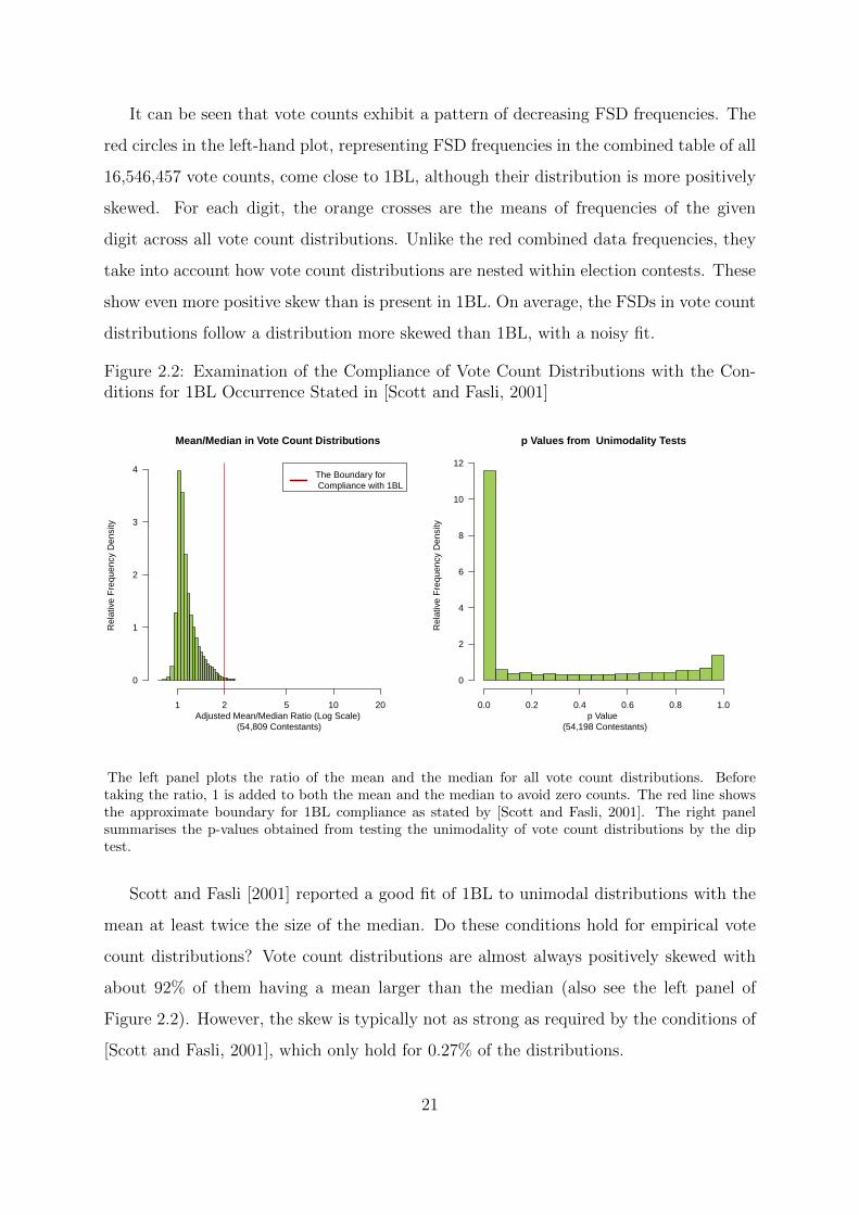
It can be seen that vote counts exhibit a pattern of decreasing FSD frequencies. The
red circles in the left-hand plot, representing FSD frequencies in the combined table of all
16,546,457 vote counts, come close to 1BL, although their distribution is more positively
skewed. For each digit, the orange crosses are the means of frequencies of the given
digit across all vote count distributions. Unlike the red combined data frequencies, they
take into account how vote count distributions are nested within election contests. These
show even more positive skew than is present in 1BL. On average, the FSDs in vote count
distributions follow a distribution more skewed than 1BL, with a noisy fit.
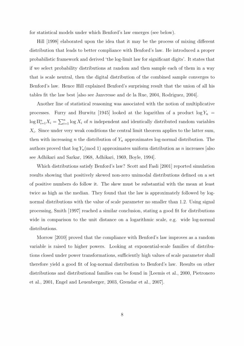
Figure 2.2: Examination of the Compliance of Vote Count Distributions with the Con-ditions for 1BL Occurrence Stated in [Scott and Fasli, 2001]
1 2 5 10 20
0
1
2
3
4
Mean/Median in Vote Count Distributions
Adjusted Mean/Median Ratio (Log Scale) (54,809 Contestants)
Rel
ativ
e F
requ
ency
Den
sity
The Boundary for Compliance with 1BL
0.0 0.2 0.4 0.6 0.8 1.0
0
2
4
6
8
10
12
p Values from Unimodality Tests
p Value (54,198 Contestants)
Rel
ativ
e F
requ
ency
Den
sity
The left panel plots the ratio of the mean and the median for all vote count distributions. Beforetaking the ratio, 1 is added to both the mean and the median to avoid zero counts. The red line showsthe approximate boundary for 1BL compliance as stated by [Scott and Fasli, 2001]. The right panelsummarises the p-values obtained from testing the unimodality of vote count distributions by the diptest.
Scott and Fasli [2001] reported a good fit of 1BL to unimodal distributions with the
mean at least twice the size of the median. Do these conditions hold for empirical vote
count distributions? Vote count distributions are almost always positively skewed with
about 92% of them having a mean larger than the median (also see the left panel of
Figure 2.2). However, the skew is typically not as strong as required by the conditions of
[Scott and Fasli, 2001], which only hold for 0.27% of the distributions.
21
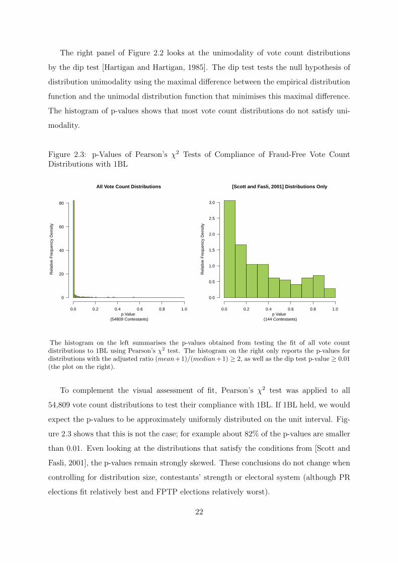
The right panel of Figure 2.2 looks at the unimodality of vote count distributions
by the dip test [Hartigan and Hartigan, 1985]. The dip test tests the null hypothesis of
distribution unimodality using the maximal difference between the empirical distribution
function and the unimodal distribution function that minimises this maximal difference.
The histogram of p-values shows that most vote count distributions do not satisfy uni-
modality.
Figure 2.3: p-Values of Pearson’s χ2 Tests of Compliance of Fraud-Free Vote CountDistributions with 1BL
0.0 0.2 0.4 0.6 0.8 1.0
0
20
40
60
80
All Vote Count Distributions
p Value (54809 Contestants)
Rel
ativ
e F
requ
ency
Den
sity
0.0 0.2 0.4 0.6 0.8 1.0
0.0
0.5
1.0
1.5
2.0
2.5
3.0
[Scott and Fasli, 2001] Distributions Only
p Value (144 Contestants)
Rel
ativ
e F
requ
ency
Den
sity
The histogram on the left summarises the p-values obtained from testing the fit of all vote countdistributions to 1BL using Pearson’s χ2 test. The histogram on the right only reports the p-values fordistributions with the adjusted ratio (mean+1)/(median+1) ≥ 2, as well as the dip test p-value ≥ 0.01(the plot on the right).
To complement the visual assessment of fit, Pearson’s χ2 test was applied to all
54,809 vote count distributions to test their compliance with 1BL. If 1BL held, we would
expect the p-values to be approximately uniformly distributed on the unit interval. Fig-
ure 2.3 shows that this is not the case; for example about 82% of the p-values are smaller
than 0.01. Even looking at the distributions that satisfy the conditions from [Scott and
Fasli, 2001], the p-values remain strongly skewed. These conclusions do not change when
controlling for distribution size, contestants’ strength or electoral system (although PR
elections fit relatively best and FPTP elections relatively worst).
22
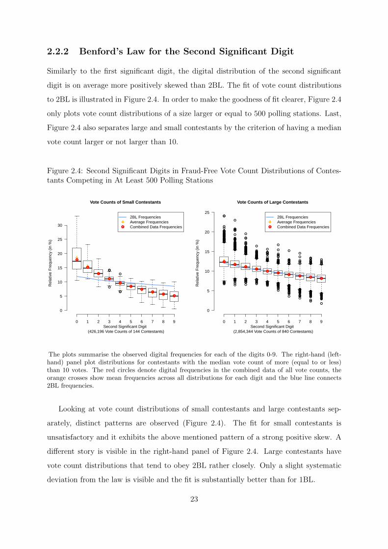
2.2.2 Benford’s Law for the Second Significant Digit
Similarly to the first significant digit, the digital distribution of the second significant
digit is on average more positively skewed than 2BL. The fit of vote count distributions
to 2BL is illustrated in Figure 2.4. In order to make the goodness of fit clearer, Figure 2.4
only plots vote count distributions of a size larger or equal to 500 polling stations. Last,
Figure 2.4 also separates large and small contestants by the criterion of having a median
vote count larger or not larger than 10.
Figure 2.4: Second Significant Digits in Fraud-Free Vote Count Distributions of Contes-tants Competing in At Least 500 Polling Stations
●
●●
●●
●
Vote Counts of Small Contestants
Second Significant Digit (426,196 Vote Counts of 144 Contestants)
Rel
ativ
e F
requ
ency
(in
%)
0 1 2 3 4 5 6 7 8 9
0
5
10
15
20
25
30
●
●
●
●
●
●●
●●
●
●
2BL FrequenciesAverage FrequenciesCombined Data Frequencies
●
●●
●
●
●●●
●
●●
●●
●
●
●●
●
●●
●
●●
●
●
●●
●
●●●
●●
●
●
●
●●
●
●
●
●
●●
●
●
●
●●
●●
●
●●
●
●
●●
●●
●●
●
●
●
●
●
●
●
●
●
●●
●
●
●
●●●
●
●
●
●
●●
●
●
●●●
●
●
●
●
●
●●
●
●●
●
●
●
●
● ●●●
●
●
●
●
●
●●●
●
●
●
●
●
●
●
●
●
●
●
●
●
●
●
●●●
●
●
●
●
●
●●
●
●●
●
●
●●
●
●
●
●
●
●
●●
●●
●●
●●●
●
●
●
●
●
●●
●●●●●●●●●
●
●●●
●
●●●
●●
●●
●
●
●
●●
●●
●●●●
●
●
●●●● ●
●
●●
●●
●●
●
●
●
●
●
●
●
●
●●
●●
●
●
●
●
●
●
●
●
●
●●
●
●
●
●●
●●●
●
●
●●
●
●●
●●●●●
●
●
●●●
●●
●●●●●
●
●
●●●●
●
●●
●●
●
●
●●
●
●
●●
●
●
●
●
●
●
●●
●●●
●
●
●●
●
●
●
●
●
●●●
●
●●
●●
●●
●●
●●
●
●
●
●
●●
●
●
●
●●●
●
●●●●
●
●
●
●
●
●
●
●●
●●
●
●
●
● ●
●●
●
●●●
●
●●●●
●●
●
●
●●
●
●
●
●●
●●●●
●
●●
●
●●●
●
●
●
●
●●●●
●
●●●●●
●
●
●
●●●●
●●●●●●●
●●
●
●
●●●
●●
●●
●●●●●●
●
●●●●●●
●
●
●
●
●
●
●
●●
●
●
●
●●●●●
●●
Vote Counts of Large Contestants
Second Significant Digit (2,854,344 Vote Counts of 840 Contestants)
Rel
ativ
e F
requ
ency
(in
%)
0 1 2 3 4 5 6 7 8 9
0
5
10
15
20
25
●●
●●
●●
●● ●
●
●
2BL FrequenciesAverage FrequenciesCombined Data Frequencies
The plots summarise the observed digital frequencies for each of the digits 0-9. The right-hand (left-hand) panel plot distributions for contestants with the median vote count of more (equal to or less)than 10 votes. The red circles denote digital frequencies in the combined data of all vote counts, theorange crosses show mean frequencies across all distributions for each digit and the blue line connects2BL frequencies.
Looking at vote count distributions of small contestants and large contestants sep-
arately, distinct patterns are observed (Figure 2.4). The fit for small contestants is
unsatisfactory and it exhibits the above mentioned pattern of a strong positive skew. A
different story is visible in the right-hand panel of Figure 2.4. Large contestants have
vote count distributions that tend to obey 2BL rather closely. Only a slight systematic
deviation from the law is visible and the fit is substantially better than for 1BL.
23
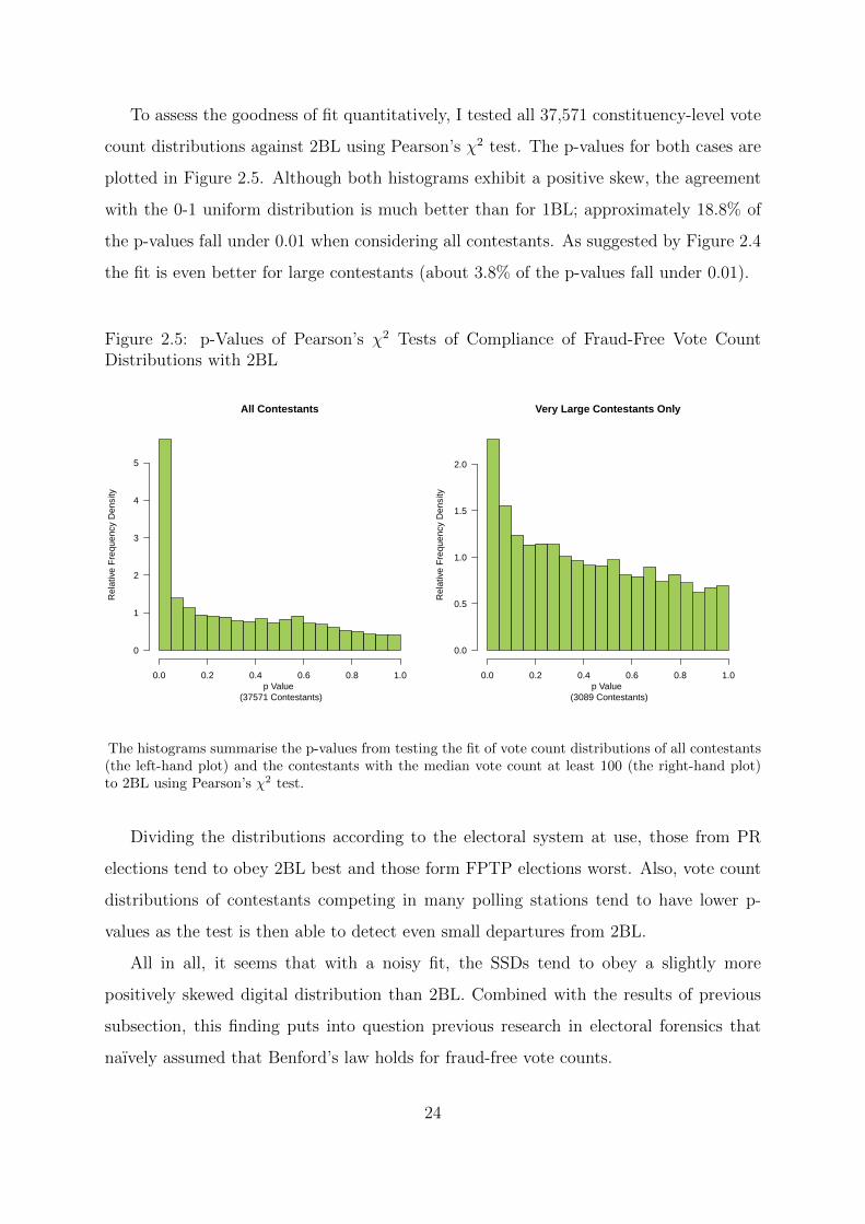
To assess the goodness of fit quantitatively, I tested all 37,571 constituency-level vote
count distributions against 2BL using Pearson’s χ2 test. The p-values for both cases are
plotted in Figure 2.5. Although both histograms exhibit a positive skew, the agreement
with the 0-1 uniform distribution is much better than for 1BL; approximately 18.8% of
the p-values fall under 0.01 when considering all contestants. As suggested by Figure 2.4
the fit is even better for large contestants (about 3.8% of the p-values fall under 0.01).
Figure 2.5: p-Values of Pearson’s χ2 Tests of Compliance of Fraud-Free Vote CountDistributions with 2BL
0.0 0.2 0.4 0.6 0.8 1.0
0
1
2
3
4
5
All Contestants
p Value (37571 Contestants)
Rel
ativ
e F
requ
ency
Den
sity
0.0 0.2 0.4 0.6 0.8 1.0
0.0
0.5
1.0
1.5
2.0
Very Large Contestants Only
p Value (3089 Contestants)
Rel
ativ
e F
requ
ency
Den
sity
The histograms summarise the p-values from testing the fit of vote count distributions of all contestants(the left-hand plot) and the contestants with the median vote count at least 100 (the right-hand plot)to 2BL using Pearson’s χ2 test.
Dividing the distributions according to the electoral system at use, those from PR
elections tend to obey 2BL best and those form FPTP elections worst. Also, vote count
distributions of contestants competing in many polling stations tend to have lower p-
values as the test is then able to detect even small departures from 2BL.
All in all, it seems that with a noisy fit, the SSDs tend to obey a slightly more
positively skewed digital distribution than 2BL. Combined with the results of previous
subsection, this finding puts into question previous research in electoral forensics that
naıvely assumed that Benford’s law holds for fraud-free vote counts.
24
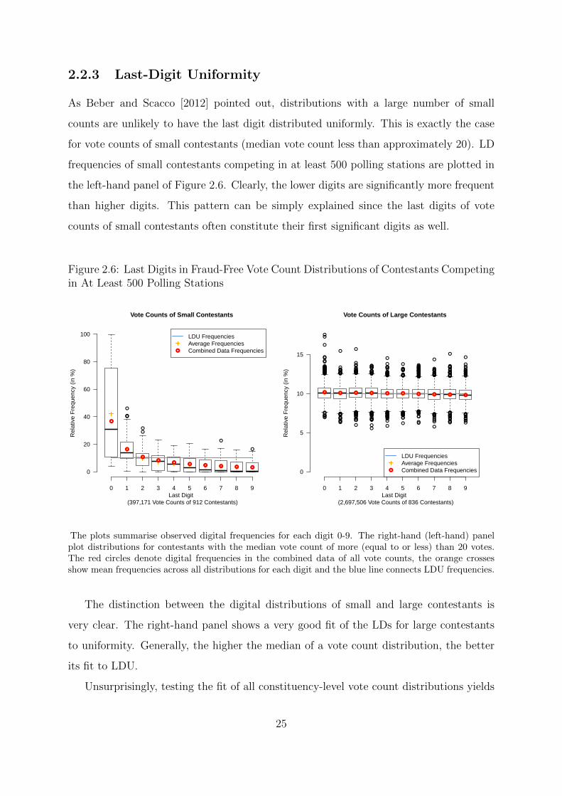
2.2.3 Last-Digit Uniformity
As Beber and Scacco [2012] pointed out, distributions with a large number of small
counts are unlikely to have the last digit distributed uniformly. This is exactly the case
for vote counts of small contestants (median vote count less than approximately 20). LD
frequencies of small contestants competing in at least 500 polling stations are plotted in
the left-hand panel of Figure 2.6. Clearly, the lower digits are significantly more frequent
than higher digits. This pattern can be simply explained since the last digits of vote
counts of small contestants often constitute their first significant digits as well.
Figure 2.6: Last Digits in Fraud-Free Vote Count Distributions of Contestants Competingin At Least 500 Polling Stations
●
●●
●●
●
●
Vote Counts of Small Contestants
Last Digit (397,171 Vote Counts of 912 Contestants)
Rel
ativ
e F
requ
ency
(in
%)
0 1 2 3 4 5 6 7 8 9
0
20
40
60
80
100
●
●
●●
● ● ● ● ● ●
●
LDU FrequenciesAverage FrequenciesCombined Data Frequencies
●●●●●●
●
●●
●
●
●
●
●
●
●
●●●●
●
●
●
●●
●●
●●●●●●●
●●
●●
●
●●
●●
●
●
●
●●●
●
●
●
●
●
●
●●●
●
●
●
●
●
●
●●●
●
●●●
●
●
●
●
●
●
●
●●
●●
●
●●
●
●
●
●
●
●
●●
●
●
●●
●
● ●
●
●
●
●
●
●
●
●
●
●
●
●
●
●
●
●
●●●●●
●●
●
●
●●
●
●
●
●
●
●
●
●
●
●
●
●●
●
●
●●●●●
●●●
●
●
●
●
●
●
●
●
●●●●
●
●
●
●●
●●
●
●
●● ●●●●
●●
●
●●●
●
●
●
●
●
●
●
●
●
●
●
●
●
●●
●
●●●
●
●
●●●
●
●
●
●●
●●●
●●
●
●
●
●
●●●
●●●
●
●
●●
●●●
●
●
●
●
●
●
●●
●●
●
●
●
●
●
●
●●
●●
●
●
●
●
●●
●
●
●
●
●●●
●
●●●
●
●
●
●●
●
●
●
●
●
●
●
●
●
●●
●
●
●
●
●●
●
●
●
●●
●●●●
●
●
●
●●
●
●●●
●
●
●
●
●
●
●
●●
●
●
●●●●
●●
●
●●●
●
●
●
●
●
●●●
●
●
●
●●
●
●
Vote Counts of Large Contestants
Last Digit (2,697,506 Vote Counts of 836 Contestants)
Rel
ativ
e F
requ
ency
(in
%)
0 1 2 3 4 5 6 7 8 9
0
5
10
15
● ● ● ● ● ● ● ● ● ●
●
LDU FrequenciesAverage FrequenciesCombined Data Frequencies
The plots summarise observed digital frequencies for each digit 0-9. The right-hand (left-hand) panelplot distributions for contestants with the median vote count of more (equal to or less) than 20 votes.The red circles denote digital frequencies in the combined data of all vote counts, the orange crossesshow mean frequencies across all distributions for each digit and the blue line connects LDU frequencies.
The distinction between the digital distributions of small and large contestants is
very clear. The right-hand panel shows a very good fit of the LDs for large contestants
to uniformity. Generally, the higher the median of a vote count distribution, the better
its fit to LDU.
Unsurprisingly, testing the fit of all constituency-level vote count distributions yields
25
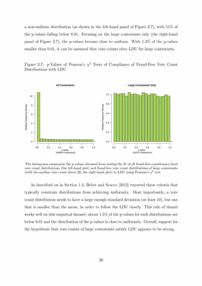
a non-uniform distribution (as shown in the left-hand panel of Figure 2.7), with 51% of
the p-values falling below 0.01. Focusing on the large contestants only (the right-hand
panel of Figure 2.7), the p-values become close to uniform. With 1.3% of the p-values
smaller than 0.01, it can be assumed that vote counts obey LDU for large contestants.
Figure 2.7: p-Values of Pearson’s χ2 Tests of Compliance of Fraud-Free Vote CountDistributions with LDU
0.0 0.2 0.4 0.6 0.8 1.0
0
2
4
6
8
10
All Contestants
p Value (54809 Contestants)
Rel
ativ
e F
requ
ency
Den
sity
0.0 0.2 0.4 0.6 0.8 1.0
0.0
0.2
0.4
0.6
0.8
1.0
Large Contestants Only
p Value (19152 Contestants)
Rel
ativ
e F
requ
ency
Den
sity
The histograms summarise the p-values obtained from testing the fit of all fraud-free constituency-levelvote count distributions (the left-hand plot) and fraud-free vote count distributions of large contestants(with the median vote count above 20, the right-hand plot) to LDU using Pearson’s χ2 test.
As described on in Section 1.4, Beber and Scacco [2012] reported three criteria that
typically constrain distributions from achieving uniformity. Most importantly, a vote
count distribution needs to have a large enough standard deviation (at least 10), but one
that is smaller than the mean, in order to follow the LDU closely. This rule of thumb
works well on this empirical dataset; about 1.5% of the p-values for such distributions are
below 0.01 and the distribution of the p-values is close to uniformity. Overall, support for
the hypothesis that vote counts of large contestants satisfy LDU appears to be strong.
26
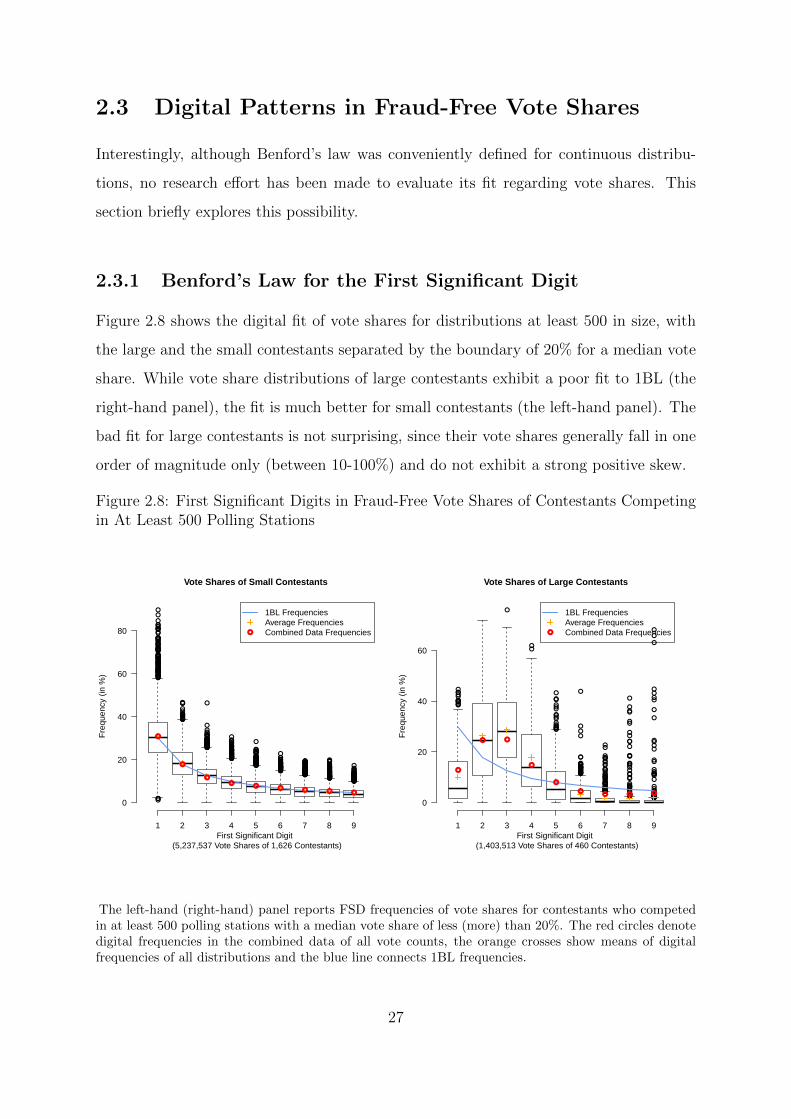
2.3 Digital Patterns in Fraud-Free Vote Shares
Interestingly, although Benford’s law was conveniently defined for continuous distribu-
tions, no research effort has been made to evaluate its fit regarding vote shares. This
section briefly explores this possibility.
2.3.1 Benford’s Law for the First Significant Digit
Figure 2.8 shows the digital fit of vote shares for distributions at least 500 in size, with
the large and the small contestants separated by the boundary of 20% for a median vote
share. While vote share distributions of large contestants exhibit a poor fit to 1BL (the
right-hand panel), the fit is much better for small contestants (the left-hand panel). The
bad fit for large contestants is not surprising, since their vote shares generally fall in one
order of magnitude only (between 10-100%) and do not exhibit a strong positive skew.
Figure 2.8: First Significant Digits in Fraud-Free Vote Shares of Contestants Competingin At Least 500 Polling Stations
●●
●
●
●
●●
●
●
●
●●●
●
●
●
●●●
●
●●
●
●
●
●
●
●
●●
●
●●
●
●●
●
●
●
●
●
●●
●●
●●
●
●
●
●
●
●
●
●
●
●
●
●●●
●
●
●
●
●
●●
●●
●
●
●●
●
●
●
●
●
●
●
●
●
●●
●
●●
●
●●
●●●
●
●●●
●●●●●●●●●●●
●●●
●
●●●●●●●●
●
●●●●
●
●●●●●●●●●●
●
●
●
●
●●●
●●●●●●●●●●●
●●●
●●●
●●●●
●
●
●●●
●
●
●
●●●
●●
●
●●
●●
●
●●●●●●
●●●●
●
●●●●●
●
●●●
●●
●
●
●●●●●●
●●●●●
●
●●●●●
●
●●●●
●●●●●●●●●
●●
●
●
●●
●
●●●●
●●●●●●
●
●●
●●●●●
●
●●●
●●●●●●●●
●
●●●●●●●●●●●●●
●●●
●●●●●●●●●●●●●
●
●
●●●●●
●●●●●●●●●●●●●
●●
●●●●●●●●●
●
●●●●
●
●
●
●●●
●
●●●●●●●●●
●●●●●●●
●
●●●●●
●●
●
●
●●●●●●●●
●●●●●●
●
●●●●●●●●●●●●
●
●
●
●●●●●●●●●●●●
●
●●●●●●●●●●●●●●●
●
●●●
●
●●●●●●
●●
●●
●
●
●
●●●●●●●
●●●●
●●●
●
●●●●●●●●
●●
●●●●●
●
●
●●
●●●●●
●●●●●●●●●●●●●●●●●●●●●●
●
●●●●●●●●●●●●●
●
●●●●
●●
●
●
●●●●●●●●
●
●●●●●●●
●
Vote Shares of Small Contestants
First Significant Digit (5,237,537 Vote Shares of 1,626 Contestants)
Fre
quen
cy (
in %
)
1 2 3 4 5 6 7 8 9
0
20
40
60
80
●
●
●●
● ● ● ● ●
●
1BL FrequenciesAverage FrequenciesCombined Data Frequencies
●●●●●●●●
●
●
●
●
●
●
●●
●●
●●
●
●●
●
●
●
●
●
●
●
●●●●
●●●
●●
●●●●●
●
●
●●●●
●●●
●
●●●●●●●
●
●●●●●●
●●
●
●
●
●
●
●●●●●●●
●
●
●●●●●●●●●●●●●●●
●
●●
●
●
●
●
●
●
●●
●
●
●
●
●
●
●
●●
●●●●
●
●
●
●●
●●●●●●●●●●
●●
●●●
●
●
●●
●
●
●
●
●
●
●
●
●
●
●●
●
●
●
●
●●
●
●
●
●
●● ●
●●●●●●●●●●●●●●●●●●●●●●●●●●
●
●
●●
●
●
●●
●
●●
●
●
●
●
●
●
●
●
●
●
●
●
●
●●
●●
Vote Shares of Large Contestants
First Significant Digit (1,403,513 Vote Shares of 460 Contestants)
Fre
quen
cy (
in %
)
1 2 3 4 5 6 7 8 9
0
20
40
60
●
● ●
●
●
●● ● ●
●
1BL FrequenciesAverage FrequenciesCombined Data Frequencies
The left-hand (right-hand) panel reports FSD frequencies of vote shares for contestants who competedin at least 500 polling stations with a median vote share of less (more) than 20%. The red circles denotedigital frequencies in the combined data of all vote counts, the orange crosses show means of digitalfrequencies of all distributions and the blue line connects 1BL frequencies.
27
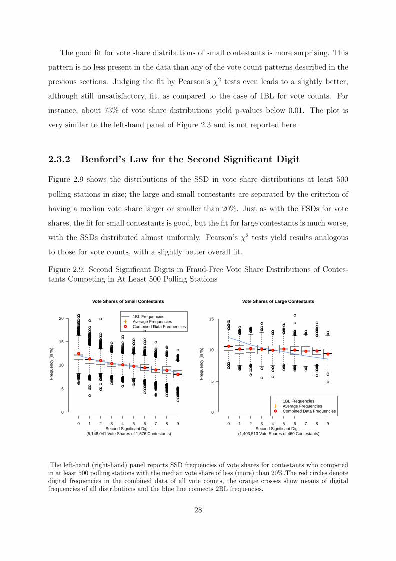
The good fit for vote share distributions of small contestants is more surprising. This
pattern is no less present in the data than any of the vote count patterns described in the
previous sections. Judging the fit by Pearson’s χ2 tests even leads to a slightly better,
although still unsatisfactory, fit, as compared to the case of 1BL for vote counts. For
instance, about 73% of vote share distributions yield p-values below 0.01. The plot is
very similar to the left-hand panel of Figure 2.3 and is not reported here.
2.3.2 Benford’s Law for the Second Significant Digit
Figure 2.9 shows the distributions of the SSD in vote share distributions at least 500
polling stations in size; the large and small contestants are separated by the criterion of
having a median vote share larger or smaller than 20%. Just as with the FSDs for vote
shares, the fit for small contestants is good, but the fit for large contestants is much worse,
with the SSDs distributed almost uniformly. Pearson’s χ2 tests yield results analogous
to those for vote counts, with a slightly better overall fit.
Figure 2.9: Second Significant Digits in Fraud-Free Vote Share Distributions of Contes-tants Competing in At Least 500 Polling Stations
●●●
●
●
●●●
●
●●
●●
●●●
●
●
●
●
●
●
●
●
●●
●
●●
●●●
●
●●●
●
●
●
●
●●
●●●
●
●
●
●●
●●
●
●
●●
●●
●●
●
●
●
●●
●
●
●●
●●
●
●●
●
●
●
●●
●
●
●
●
●
●●●●
●
●●
●
●
●●
●
●
●●
●●
●
●
●
●
●●
●
●●●
●
●
●
●
●
●
●
●
●●●
●
●●●
●
●
●
●
●
●
●●
●
●
●
●
●●●●
●
●●
●
●●
●●
●
●
●●
●●●●●
●
●
●
●●
●
●
●
●
●
●
●
●
●●●
●●
●
●
●
●
●●
●●
●
●
●
●
●
●●
●
●
●
●
●
●
●
●
●
●
●●
●●
●
●●
●●●●●●
●
●●
●●●
●●●●
●●
●●
●
●
●
●●●
●
●
●
●●
●
●
●●●
●
●
●●●
●●●●
●●●●●●
●
●
●●
●
●●●
●●
●●
●●
●
●
●
●
●
●●
●
●
●
●
●
●
●
●
●
●
●
●●
●
●
●●
●
●●
●
●
●
●●
●
●●
●
●
●●
●●●
●●●●●
●
●
●●●
●
●
●
●
●
●
●●
●●●●●
●●●
● ●
●
●
●
●●
●
●
●
●●
●
●
●
●●
●●
●
●
●
●
●●
●●●
●
●
●
●
●●●●●●
●
●
●
●
●
●
●
●
●●
●
●●
●
●
●●
●●
●
●●●
●
●
●
●
●
●
●
●
●
●
●
●
●●
●●
●
●
●
●●
●
●
●
●
●●
●●
●●
●
●
●●
●●●
●●●
●
●
●
●
●●
●
●
●●
●●●●●
●
●●
●
●●●
●
●
●●
●
●●
●
●
●
●
●
●
●
●
●●
●●●●
●
●
●
●●
●
●●●●
●
●
●
●
●●
●●●
●
●
●
●
●
●
●●●
●
●
●
●
●●●
●●
●
●●
●●●
●
●●●
●
●●●●
●●●●
●
●
●
●●●
●
●
●●
●
●●
●
●
●
●
●●
●●
●●
●
●●●
●●
●●
●●
●
●
●
●
●
●
●●●●
●●
●
●
●●●●
●
●
●
●
●●●
●
●
●●
●●●
●
●●●●●
●●
●●●
●●
●
●●
●
●
●
●
●●●
●
●●
●●
●●
●●
●●
Vote Shares of Small Contestants
Second Significant Digit (5,148,041 Vote Shares of 1,576 Contestants)
Fre
quen
cy (
in %
)
0 1 2 3 4 5 6 7 8 9
0
5
10
15
20
●
●●
●●
●●
● ●
●
●
1BL FrequenciesAverage FrequenciesCombined Data Frequencies
●
●
●●
●
●
●●
●
●●
●
●●●
●●●
●
●
●
●
●
●●●
●
●
●
●
●●
●●
●
●
●●●
●
●
●●●
●●●●
●●
●●● ●
●
●
●
●
●●●
●
●
●●
●●
● ●
●
●●
●
●●
●
●
●
●
●
● ●
●●●
●
●●
●●
●●
●●
●
●
●
●
●●●
●
●●●
●●●
●●
●
●
●●
●
●
●
●
●
●●
●●●
●
●
●
●
●
●
●●
●
●
●
●
●
●
●
●
Vote Shares of Large Contestants
Second Significant Digit (1,403,513 Vote Shares of 460 Contestants)
Fre
quen
cy (
in %
)
0 1 2 3 4 5 6 7 8 9
0
5
10
15
●● ● ● ● ● ● ● ●
●
●
1BL FrequenciesAverage FrequenciesCombined Data Frequencies
The left-hand (right-hand) panel reports SSD frequencies of vote shares for contestants who competedin at least 500 polling stations with the median vote share of less (more) than 20%.The red circles denotedigital frequencies in the combined data of all vote counts, the orange crosses show means of digitalfrequencies of all distributions and the blue line connects 2BL frequencies.
28
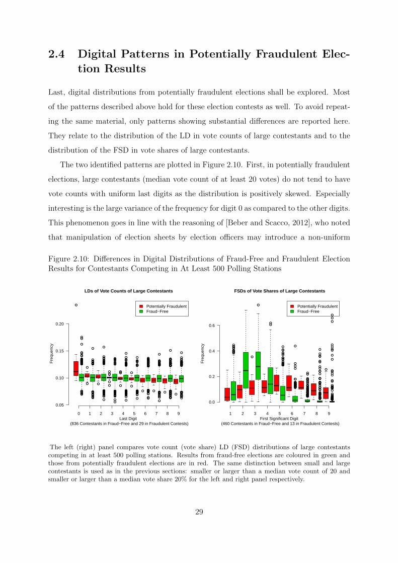
2.4 Digital Patterns in Potentially Fraudulent Elec-
tion Results
Last, digital distributions from potentially fraudulent elections shall be explored. Most
of the patterns described above hold for these election contests as well. To avoid repeat-
ing the same material, only patterns showing substantial differences are reported here.
They relate to the distribution of the LD in vote counts of large contestants and to the
distribution of the FSD in vote shares of large contestants.
The two identified patterns are plotted in Figure 2.10. First, in potentially fraudulent
elections, large contestants (median vote count of at least 20 votes) do not tend to have
vote counts with uniform last digits as the distribution is positively skewed. Especially
interesting is the large variance of the frequency for digit 0 as compared to the other digits.
This phenomenon goes in line with the reasoning of [Beber and Scacco, 2012], who noted
that manipulation of election sheets by election officers may introduce a non-uniform
Figure 2.10: Differences in Digital Distributions of Fraud-Free and Fraudulent ElectionResults for Contestants Competing in At Least 500 Polling Stations
●
●●●●●●
●
●●
●
●
●
●
●
●
●
●●●●
●
●
●
●●
●●
●●●●●●●
●●
●●
●
●
●
●
●
●●
●
●
●
●●●
●
●
●
●
●
●
●●●
●
●
●
●
●
●
●
●●●
●
●●●
●
●
●
●
●
●
●
●●
●●
●
●●
●
●
●
●
●
●
●●
●
●
●●
●
●
●
●
●●●
●
●
●
●
●
●
●
●
●
●
●
●
●
●
●
●
●
●●●●●
●●
●
●
●●
●
●
●
●
●
●
●●●
●
●
●
●
●
●
●●
●
●
●●●●●
●●●
●
●
●
●
●
●
●
●
●●●●
●
●
●
●●
●●
●
●
●●
●
●
●●●●●●
●
●●●
●
●
●
●
●
●
●
●
●
●
●
●
●
●●
●
●●●
●●
●
●●●
●
●
●
●●
●●●
●●
●
●
●
●
●●●
●●●
●
●
●●
●●●
●
●
●
●
●
●
●●
●●
●
●
●
●●
●●
●●
●●
●
●
●
●
●●
●
●
●
●
●●●
●
●●●
●
●
●
●
●●
●
●
●
●
●
●
●
●
●
●●
●
●
●
●
●●
●
●
●
●●
●●●●
●
●
●
●●
●
●●●
●
●
●
●
●
●
●
●
●●
●
●
●●●●
●●
●
●●●
●
●
●
●
●
●●●
●
●
●
●●
●
●
LDs of Vote Counts of Large Contestants
Last Digit (836 Contestants in Fraud−Free and 29 in Fraudulent Contests)
Fre
quen
cy
Potentially FraudulentFraud−Free
0 1 2 3 4 5 6 7 8 9
0.05
0.10
0.15
0.20
●●●●●●●●
●
●
●
●
●
●
●
●●
●●
●●
●
●●
●
●
●
●
●
●
●
●●●●
●●●
●●
●●●●●
●
●
●●●●
●●●
●
●●●●●●●
●
●●●●●●
●●
●
●
●
●
●
●●●●●●●
●
●
●●●●●●●●●●●●●●●
●
●●
●
●
●
●
●
●
●●
●
●
●
●
●
●
●
●●
●●●●
●
●
●
●●
●●●●●●●●●●
●●
●●●
●
●
●●
●
●
●
●
●
●
●
●
●
●
●●
●
●
●
●
●●
●
●
●
●
●●
●
●
●●●●●●●●●●●●●●●●●●●●●●●●●●
●
●
●●
●
●
●●
●
●●
●
●
●
●
●
●
●
●
●
●
●
●
●
●●
●●
FSDs of Vote Shares of Large Contestants
First Significant Digit (460 Contestants in Fraud−Free and 13 in Fraudulent Contests)
Fre
quen
cy
Potentially FraudulentFraud−Free
1 2 3 4 5 6 7 8 9
0.0
0.2
0.4
0.6
The left (right) panel compares vote count (vote share) LD (FSD) distributions of large contestantscompeting in at least 500 polling stations. Results from fraud-free elections are coloured in green andthose from potentially fraudulent elections are in red. The same distinction between small and largecontestants is used as in the previous sections: smaller or larger than a median vote count of 20 andsmaller or larger than a median vote share 20% for the left and right panel respectively.
29

pattern into the LD distribution.
Second, large contestants (median vote share of at least 20%) tend to have a vote share
FSD digit distribution much flatter than that of contestants in fraud-free elections. This
pattern may be related to the fact that the vote shares of large contestants in fraudulent
elections are artificially increased and therefore tend to be higher than vote shares in
fraud-free elections.
All in all, some distinctions in the digital patterns have been identified. Interestingly,
the most widely adopted digital patterns in election forensics (1BL and 2BL for vote
counts) do not yield substantial differences. However, it must be stressed that the number
of potentially fraudulent contests included is small, and the conclusions of this subsection
should by no means be regarded as definitive.
30
Chapter 3
Synthetic Data Analysis
This chapter aims to assess the usefulness of digital patterns for separating fraud-free
and fraudulent electoral contests. Empirical data cannot be used for this purpose for two
main reasons. First, election results (as defined in Subsection 1.1) are rarely available
for fraudulent elections. Second, the degree or even the very presence of election fraud is
inherently unobservable.
Due to these two reasons, simulations are more suitable for the assessment of the
potential and limits of digital election forensics. If data mimicking election contests can
be simulated, then election fraud can be artificially introduced into their subsets and
supervised machine learning procedures can be used to classify the simulated contests
according to their type. In the following, Section 3.1 describes how fraud-free election
results can be modelled, Section 3.2 reports the design implemented for data simulation
and evaluates the goodness of digital fit of the synthetic data to the empirical data.
Finally, Section 3.3 reports the results from applying a logistic learner to the simulated
data.
31
3.1 Models for Election Results
As in all contests, election contests feature more than one contestant. Therefore, election
contest modelling constitutes a compositional problem, i.e. the election results of the
contestants represent interrelated portions of a whole. Surprisingly, previous simulational
studies in digital election forensics did not take the compositional nature of election results
into account [see Myagkov et al., 2009, Mebane, 2010a,b, Cantu and Saiegh, 2011]. This
dissertation adopts a compositional approach to election results modelling.
Two main approaches to compositionally approximate election results exist: either
vote counts or vote shares are modelled. A standard way of simulating vote counts is
by multinomial distribution [see Wand et al., 2001a,b, Mebane and Sekhon, 2004], and
a standard way of modelling vote shares is by a compositional framework introduced in
[Aitchison, 1986], namely the recently refined concept of additive logistic normal distri-
butions [see Katz and King, 1999]. These two approaches are explained in more detail
below. For alternatives see [Jackson, 2002] and [Linzer, 2012].
3.1.1 Theoretical Framework
This subsection defines the compositional terms needed for model description. It is
predominantly based on [van den Boogaart and Tolosana-Delgado, 2013].
As mentioned earlier, by a composition or a D-composition x = (x1, x2, . . . , xD), I
mean a data point of D portions of the total. Individual values xj, with j ∈ {1, . . . , D},
of a D-composition are denoted as amounts and each of them is associated with a single
element of the composition. Summing the amounts of all the elements in a composition
gives the total amount or the total t. Finally, amounts xj divided by the total amount
are called portions and denoted by pj.
It is obvious that taking both the D vote counts or vote shares from a single polling
station yields a composition with D elements (contestants). Vote counts cj constitute
the amounts, and the total number of valid votes cast in the given polling station is the
total t. Vote shares sj = cj/t represent portions of the composition.
More generally, the transformation of amounts into portions is called the closure of a
32

composition and is defined by operation: C(x) = 1t
(x1, x2, . . . , xD). A composition x is
called a closed composition if a composition y exists such that C(y) = x. The set of all
possible closed D-compositions, i.e. the following:
SD =
{x = (x1, x2, . . . , xD)i=1,...,D : xi ≥ 0,
D∑i=1
xi = 1
}
is called the D-part simplex. The D-part simplex therefore constitutes the set of all
possible vote share compositions of D contestants.
Three operations on the D-part simplex will be needed. Perturbation x ⊕ y of com-
positions x and y is the closure of their component-wise product:
x⊕ y = C(x1 · y1, . . . , xD · yD),
powering λ� x of composition x by scalar λ is the closure of its component-wise powers
to the λ:
λ� x = C(xλ1 , . . . , xλD),
and the Aitchison scalar product 〈x,y〉A of compositions x and y is defined as:
〈x,y〉A =1
D
D∑i>j
logxixj
logyiyj.
It can be shown that the D-part simplex together with perturbation, powering and the
Aitchison scalar product defines a (D− 1)-dimensional Euclidean space structure on the
simplex [Pawlowsky-Glahn, 2003, van den Boogaart and Tolosana-Delgado, 2013, p. 37-
41]. Statistical modelling on the simplex using these operations is therefore equivalent
to statistical modelling in RD−1. Using isometric1 transformations, the vote shares of
D contestants can be transformed into RD−1, standard multivariate techniques can be
applied there and the results can be re-transformed into the original simplex.
One standard isometric linear mapping is called isometric log-ratio transformation. If
V is a D × (D − 1) matrix with its columns constituted by D − 1 normalised linearly
1Transformations preserving angles and distances as defined in [van den Boogaart and Tolosana-Delgado, 2013, p. 40].
33
independent vectors orthogonal to 1 = (1, . . . , 1), then we define ilr : SD → RD−1 as:
y = ilr(x) := log(x) ·VT
with the inverse transformation x = C [exp(y ·V)] . ilr() induces the Aitchison measure
λS = λ ({ilr(x) : x ∈ A}) for the simplex, analogous to the Lebesgue-measure λ [van den
Boogaart and Tolosana-Delgado, 2013, p. 43].
3.1.2 A Model for Vote Shares
Using the above methodology, we can define a model for vote share compositions [see
van den Boogaart and Tolosana-Delgado, 2013, p. 51-53]. A random vote share com-
position S has a normal distribution on the simplex NS(m,Σ) with mean vector m and
variance matrix Σ if projecting it onto any arbitrary direction of the simplex u with the
Aitchison scalar product leads to a random variable with univariate normal distribution,
of mean vector 〈m,u〉A and variance clr(u) ·Σ · [clr(u)]T . Taking V as the basis of the
simplex, the coordinates ilr(s) of random vote share composition S have the following
joint density with respect to the Aitchison measure λS:
f(s;µV ,ΣV ) =1√
(2π)D−1 · |ΣV |exp
[−1
2(ilr(s)− µV ) ·Σ−1V · (ilr(s)− µV )T
](3.1)
which is a multivariate normal distribution with mean vector µV and variance matrix
ΣV . Normal distribution on the simplex (NDS) was first defined by [Pawlowsky-Glahn,
2003] and it is probabilistically equivalent to the additive logistic normal distribution
introduced by [Aitchison, 1986].
A practical problem arises with fitting the NDS, since computing ilr(s) = log(s) ·VT
requires non-zero vote shares. However, zero vote counts are very common. As is usually
done, in order to overcome this technical obstacle, one vote is added to all observed vote
counts, and adjusted vote shares s′ are computed based on the adjusted vote counts c′
(summing up to the adjusted total t′).
One more adjustment has to be performed before fitting the NDS. Vote shares in
empirical datasets are often not independent of vote totals (e.g. some contestants are
34
more successful in towns where polling stations tend to be larger and vice versa). The
most straightforward way to account for this effect is by using a simple linear model
for random vote share composition S′i with the logarithm of the vote total log(t′i) as a
predictor:
S′i = a⊕ log(t′i)� b + εi (3.2)
where a and b are to-be-estimated compositional constants and εi ∼ NDS (1,Σ) is random
compositional noise. The logarithm of the vote total is used instead of simple vote totals
in order to decrease the leverage of huge polling stations, since the distribution of vote
totals is virtually always positively skewed. Interpretation of parameters a and b is of no
importance to us as the model serves for data generation only.
Following [van den Boogaart and Tolosana-Delgado, 2013, p. 129-131], Equation 3.2
can be rewritten as:
ilr(S′i) = ilr(a) + t′i · ilr(b) + ilr(εi) (3.3)
with ilr(εi) ∼ N (0D−1,Σilr). This is a standard linear model that can be fitted by
maximum likelihood using R packages stats and compositions.
3.1.3 A Multinomial Model for Vote Counts
The multinomial distribution provides a simple and intuitive way of modelling discrete
compositions [van den Boogaart and Tolosana-Delgado, 2013, p. 62-63]. Therefore it can
be conveniently used to model vote counts conditional on the total number of valid votes
cast. The probability of observing vote count composition c = (c1, c2, . . . , cD) in a polling
station with D contestants and the vote total of t is:
f(c; p, t) = t!D∏j=1
pcjj
cj!(3.4)
where p = (p1, p2, . . . , pD) are the probabilities of any vote being cast for contestants
1, . . . , D. It is assumed that all votes within a polling station are independent with the
same p (expected counts are then t · p). Since p can be interpreted as expected vote
share composition then it can be estimated using predicted vote share compositions s′
35

from Equation 3.2. A potential problem with this distribution is that since the variance
matrix t · (diag(p) − pTp) is fully determined by p, it is often not flexible enough for
modelling complex covariance structures.2
2 diag(p) stands for a matrix with p on the main diagonal and zeros elsewhere.
36

3.2 Synthetic Data Generation
This section introduces the methodology of the simulational part of the analysis. Subsec-
tion 3.2.1 describes two ways fraud-free data are herein simulated and Subsection 3.2.2
compares the goodness of digital fit of the two models. Subsection 3.2.3 introduces the
simple model of fraud imputation into the simulated fraud-free election results and Sub-
section 3.2.4 reports how logistic regression models for discrimination between fraud-free
and fraudulent results are set up.
3.2.1 Fraud-Free Data Simulation
Based on the previous section, two ways of simulating election results are considered
here. Both approaches start with fitting the NDS model defined by Equation 3.2 to the
observed vote shares.
The first approach simulates vote counts in polling station i as draws from multinomial
distribution with the total given by vote total ti and the probability vector pi given by s′i
(as defined in Equation 3.4). This can be done using function rmultinom.ccomp() from
R package compositions.
The second approach rests on a simple model that will hereinafter be denoted as the
naıve model. It simulates vote counts cij of contestant j in polling station i using a
two-step procedure. First, for each polling station i, value s′∗i is computed by sampling
ilr(s′∗i ) from the model given by Equation 3.3, that is, from N (ilr(a) + t′i · ilr(b) ,Σilr),
and applying inverse ilr(). This step is implemented in rnorm.acomp() function from
R package compositions. Second, vote counts are ‘naıvely’ approximated as cij := dti ·
s′∗ije − 1, where d e stands for ceiling. Using ceiling assures that after subtraction of
the vote previously added to compute vote shares, all vote counts remain non-negative
integers. A slight inconsistency is induced by this procedure as the computed vote counts
do not need to sum exactly to the vote total. From a practical point of view, however,
these deviations are minimal.
37
3.2.2 Goodness of Fit of the Synthetic Data
Both of the models rest on the assumption that empirical vote shares can be reasonably
well modelled by the normal distribution on the simplex. This subsection starts by
validating this assumption and then moves on to comparing the digital fit for the two
models outlined above. The decision will be made as to which of the models fits the
empirical patterns better and should therefore be used for simulations.
3.2.2.1 Fit of the Normal Model for Vote Shares
The fact that vote share distributions are often unimodal and rather bell shaped made
some researchers believe that they follow a normal distribution [see Myagkov et al., 2007,
2009]. This is of course impossible as the support of vote share distributions is bounded
by 0 and 1. If normality is to be expected in vote shares, then it would be normality on
the simplex.
The goodness of fit of the multivariate normal distribution on the simplex to em-
pirical vote share compositions can be assessed in at least two ways: either statistically
tested or visually explored. Complete compositional normality can be tested by apply-
ing a multivariate normality test to the isometric log-ratio transformations of vote share
compositions. A multivariate normality test introduced by [Szekely and Rizzo, 2008] is
implemented in command acompNormalGOF.test() of package compositions and was
applied to the election contests contained in this dataset. Overall, the test almost always
rejected the null hypothesis of multivariate normality. However, more exploration is
needed as non-normality in a single direction is sufficient to reject multivariate normality.
A visual assessment of compositional multivariate normality can be done using QQ-
plots. Multivariate normality on the simplex induces univariate normality of the loga-
rithm of a ratio of any two of its elements. Plotted values of the log-ratio transforma-
tion can then be compared with the standard normal distribution. Although bivariate
marginal normality does not necessarily imply joint normality, for most practical prob-
lems this assessment is good enough [van den Boogaart and Tolosana-Delgado, 2013].
However, a thorough visual examination is particularly difficult as the number of
election contests to examine is very high. For this reason, all election contests in elec-
38
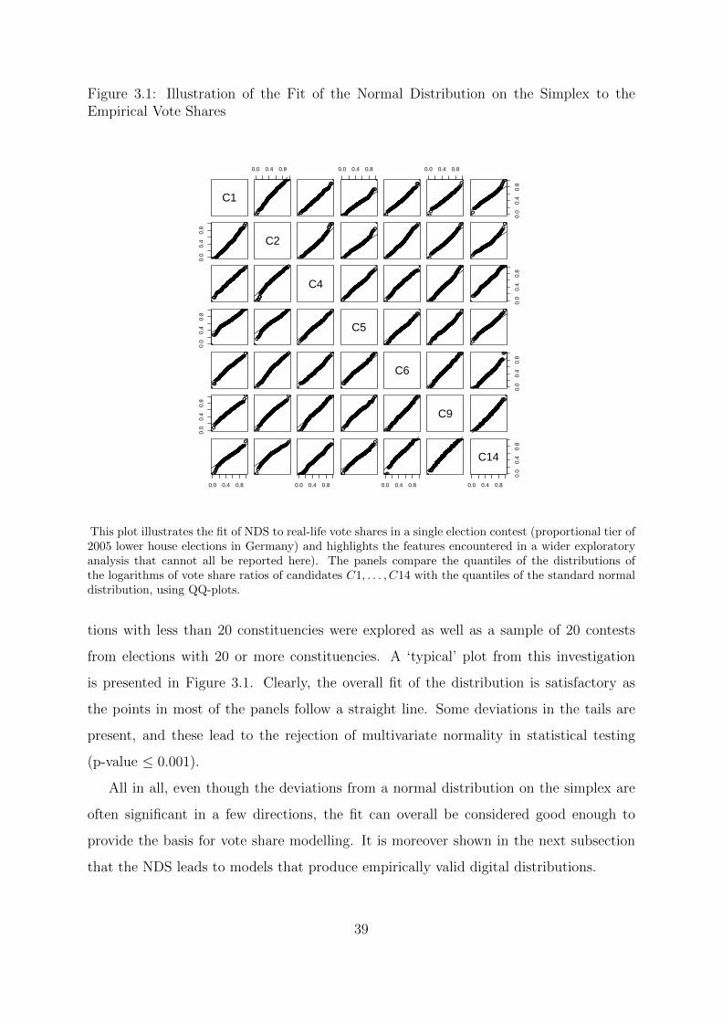
Figure 3.1: Illustration of the Fit of the Normal Distribution on the Simplex to theEmpirical Vote Shares
C1
0.0 0.4 0.8
●●●●●●●●●●●
●●●●●●●●●●●●●●●●●●●●●●●●●●●●●●●●●●●●●●●●●●●●●●●●●●●●●●●●●●●●●●●●●●●●●●●●●●●●●
●●●●●●●●●●●●●●●●●●●●●●●●●●●●●●●●●●●●●●●●●●●●●●●●●●●●●●●●●●●●●●●●●●●●●●●●●●●●●●●●●●●●●●●●●●●●●●●●●●●●●●●●●●●●●●●●●●●●●●●●●●●●●●●●●●●●●●●
●●●●●●●●●●●●●●●●●●●●●●
●●●●●●●●●
●●●
●●●●●●●●●●●●●●●●●●●●●●●●●●●
●●●●●●●●●●●●●●●●●●●●●●●●●●●●●●●●●●●●●●●●●●●●●●●●●●●●●●●●●●●●●●●●●●●●●●●●●●●●●●●●●
●●●●●●●●●●●●●●●●●●●●●●●●●●●●●●●●●●●●●●●●●●●●●●●●●●●●●●●●●●●●●●●●●●●●●●●●●●●●●●●●●●●●●●●●●●●●●●●●●●●●●●●●●
●●●●●●●●●●●●●●●●●●●●●●●●●
●●●●●●●●●●●●
●
0.0 0.4 0.8
●●●●●●●●●●●●●●●●
●●●●●●●●●●●●●●●●●●●●●●●●●●●●●●●●●●●●●●●●●●●●
●●●●●●●●●●●●●●●●●●●●●●●●●●●●●●●●●●●●●●●●●●●●●●●●●●●●●●●●●●●●●●●●●●●●●●●●●●●●
●●●●●●●●●●●●●●●●●●●●●●●●●●●●●●●●●●●●●●●●●●●●●●●●●●●●●●●●●●●●●●●●●●●●
●●●●●●●●●●●●●●●●●●●●●●●●●●●●●●●●●●●●●●●●●●●●●●●●●
●
●●●●●●●
●●●●●●●●●●●●●●●●●●●●●●●●●●●●●●●
●●●●●●●●●●●●●●●●●●●●●●●●●●●●●●●●●●●●●●●●●●●●●●●●●●●●●●●●●●●●●●●●●●●●●●●●●●●●●●●●●●●●
●●●●●●●●●●●●●●●●●●●●●●●●●●●●●●●●●●●●●●●●●●●●●●●●●●●●●●●●●●●●●●●●●●●●●●●●●●●●●●●●●●●●●●●●●●●●●●●●●●●●
●●●●●●●●●●●●●●●●●●●●●●●●●●●
●●●●
●
0.0 0.4 0.8
●●●●●●●●●●●●●●●
●●●●●●●●●●●●●●●●●●●●●●●●●●●●●●●●●●●
●●●●●●●●●●●●●●●●●●●●●●●●●●●●●●●●●●●●●●●●●●●●●●●●●●●●●●●●●●●●●●●●●●●●●●●●●●●●●●●●●●●●●●●●●●●●●●●●●●●●●●
●●●●●●●●●●●●●●●●●●●●●●●●●●●●●●●●●●●●●●●●●●●●●●●●●●●●●●●●●
●●●●●●●●●●●●●●●●●●●●●●●●●●●●●●●●●●●●●●
●●●●●
●●
0.0
0.4
0.8
●●●●●●●●
●●●●●●●●●●●●●●●●●●●●●●●●●●●●●●●●●●●●●●●●●●●●●
●●●●●●●●●●●●●●●●●●●●●●●●●●●●●●●●●●●●●●●●●●●●●●●●●●●●●●●●●●●●●●●●●●●●●●●●●●●●
●●●●●●●●●●●●●●●●●●●●●●●●●●●●●●●●●●●●●●●●●●●●●●●●●●●●●●●●●●●●●●●●●●●●●●
●●●●●●●●●●●●●●●●●●●●●●●●●●●●●●●●●●
●●●●●●●●●●●●●●●
●●●●
●●
0.0
0.4
0.8
●●●●●●●●●●●●●●●●●●●●●●●●●●●●●●●●●
●●●●●●●●●●●●●●●●●●●●●●●●●●●●●●●●●●●●●●●●●●●●●●●●●●●●●●●●●●●●●●●●●●●●●●●●●●●●●●●●●●●●●●●●●●●●●●●●●●●●●●●●●●●●●●●●●●●●●●●●●●●●●●●●●●●●●●●●●●●●●●●●●●●●●●●●●●●●●●●●●●●●●●●●●●●●●●●●●●●●●●●●●●●●●●●●●●●●●●●●●●●●●●●●●●●●●●●●●
●●●●
C2●●
●●●●●●●●●●●●●●●●●●●●●●●●●●
●●●●●●●●●●●●●●●●●●●●●●●●●●●●●●●●●●●●●●●●●●●●●●●●●
●●●●●●●●●●●●●●●●●●●●●●●●●●●●●●●●●●●●●●●●●●●●●●●●●●●●●●●●●●●●●●●
●●●●●●●●●●●●●●●●●●●●●●●●●●●●●●●●●●●●●●●●●●●●●●●●●●●●●●●●●●●●●●●●●●●●●●●●●●
●●●●●●●●●●●●●●●●●●●●●●●●●●●●●●●●●●●●●●●
●
●●●●●●●●●●●
●●●●●●●●●●●●●●●●●●●●●●●●●●●●●
●●●●●●●●●●●●●●●●●●●●●●●●●●●●●●●●●●●●●●●●●●●●●●●●●●●●●●●●●●●●●●●●●●
●●●●●●●●●●●●●●●●●●●●●●●●●●●●●●●●●●●●●●●●●●●●●●●●●●●●●●●●●●●●●●●●●●●●●●●●●●●●●●●●●
●●●●●●●●●●●●●●●●●●●●●●●●●●●●●●●●●●●●●●●
●●●●●●●●●●●●●●●●●●
●●●●●●●●
●
●
●●●●●●●●
●●●●●●●●●●●●●●●●●●●●●●●●●●●●●●●●●●●●●●●●●●●●●●●●●●●●●●●●●●●●●●●●●●●●●●●●
●●●●●●●●●●●●●●●●●●●●●●●●●●●●●●●●●●●●●●●●●●●●●●●●●●●●●●●●●●●●●●●●●●●●●●●●●●●●●●●●●●●●●●●●●●●●●●●●●●●●●●●●●●●●●●●●●●●●●●●●●●●●●●●●●●●●●●●●●●●●●●●●●●●●●●●●●●●●●●●●●●●●●●●●●●
●●●●
●●●●●
●●●●●●●●●●●●●●●●●●●
●●●●●●●●●●●●●●●●●●●●●●●●●●●●●●●●●●●●●●●●●●●●●●●●
●●●●●●●●●●●●●●●●●●●●●●●●●●●●●●●●●●●●●●●●●●●●●●●●●●●●●●●●●●●●●●●●●●●●●●●●●●●●●●●●●●●●●●●●●●●●●●●●●●●●●●●●●●●●●●●●●●●
●●●●●●●●●●●●●●●●●●●●●●●●●●●●●●●●●●●●●●●●●●●●●●●●●●●●●●●●●●●●●●●
●●●
●
●●●
●●●●●●●●●●●●●●●●●●●●●●●●●●
●●●●●●●●●●●●●●●●●●●●●●●●●●●●●●●●●●●●●●●●●●●●●●●●●●●●●●●●●
●●●●●●●●●●●●●●●●●●●●●●●●●●●●●●●●●●●●●●●●●●●●●●●●●●●●●●●●●●●●●●●●●●●●●●●●●●●●●●●
●●●●●●●●●●●●●●●●●●●●●●●●●●●●●●●●●●●●●●●●●●●●●●●●●●●●●●●●●●●●●●●●●●●●●●●
●●●●●●●●●●●●●●●●●●
●
●●●●●●●●●●●●●
●●●●●●●●●●●●●●●●●●●●●●●●●●●●●●●●●●●●●●●●●●●●●●●●●●●●●●●●●●●●●●●●●●●●●●●●●●●●●●●●●●●●●●●●●●●●●●●●●●●●●●●●●●●●●●●●●●●●●●●●●●●●●●●●●
●●●●●●●●●●●●●●●●●●●●●●●●●●●●●●●●●●●●●●●●●●●●●●●●●●●●●●●●●●●●●●●●●●●●●●●●●●●●●●●●●●
●●●●●●●●●●●●●●●●●●●●●●
●●●●●●
●
●●●●●●●●●●●●●●●●●●●●●●●●●●●●●●●●●●●●●●●●●●●●●●●●●●●●●●●●●●●●●●●●●●●●●●●●●●●
●●●●●●●●●●●●●●●●●●●●●●●●●●●●●●●●●●●●●●●●●●●●●●●●●●●●●●●
●●●●●●●●●●●●●●●●●●●●●●●●●●●●●●●●●●●●●●●●●●●●●●●●●●●●●●●●●●●●
●●●●●●●●●●●●●●●●●●●●●●●●●●●●●●●●●●●●●●●●●●
●●●●●●●●●●●●●●●●●
●●●●●
C4●
●●●●●●●●●
●●●●●●●●●●●●●●●●●●●●●●●●●●●●●●●●●
●●●●●●●●●●●●●●●●●●●●●●●●●●●●●●●●●●●●●●●●●●●●●●●●●●●●●
●●●●●●●●●●●●●●●●●●●●●●●●●●●●●●●●●●●●●●●●●●●●●●●●●●●●●●●●●●●●●●●●●●●●●●●
●●●●●●●●●●●●●●●●●●●●●●●●●●●●●●●●●●●●●●●●●●●●●●●●●●●
●●●●●●●●●●●●●●●●●●●●●●●●●●●●●
●●●●●●
●
●●●●●
●●●●●●●●●●●●●●●●●●●●●●●●●●●●●●●●●●●●●●●●●●●●●●●●●●●●●●●●●●●●●●●●●●●
●●●●●●●●●●●●●●●●●●●●●●●●●●●●●●●●●●●●●●●●●●●●●●●●●●●●●●●●●●●●●●●●●●●●●●●●●●●●●●●●●●●●●●●●●●●●●●●●●●●●●●●●●●●●●●●●
●●●●●●●●●●●●●●●●●●●●●●●●●●●●●●●●●●●●●●●●●●●●●●●●●●●●●●●●●●●
●●●●●●●●●●
●
●●●●●●●●
●●●●●●●●●●●●●●●●●●●●●●●●●
●●●●●●●●●●●●●●●●●●●●●●●●●●●●●●●●●●●●●●●●●●●●●●●●●●●●●●●●●●●●●●●●●●●
●●●●●●●●●●●●●●●●●●●●●●●●●●●●●●●●●●●●●●●●●●●●●●●●●●●●●●●●●●●●●●●●●●●●●●●●●●●●●●●●●●●●●●●●●●●●●●●●●
●●●●●●●●●●●●●●●●●●●●●●●●●●●●●●●●●●●●●●●●●●
●●●●●●●●●●●
●●●●
0.0
0.4
0.8
●
●●●●●●●●●●●●●●●●●●●●●●●●●●●●●●●●●●●●●●●●●●●●●●●●●●●●●●●●●●●
●●●●●●●●●●●●●●●●●●●●●●●●●●●●●●●●●●●●●●●●●●●●●●●●●●●●●●●●●●●●●●●●
●●●●●●●●●●●●●●●●●●●●●●●●●●●●●●●●●●●●●●●●●●●●●●●●●●●●●●●●●●●●●●●●●●●●●●●●●●●●●●
●●●●●●●●●●●●●●●●●●●●●●●●●●●●●●●●●●●●●●●●●●●●●●●●●●●●
0.0
0.4
0.8
●
●●●●●●●●●●●●●●●●●●●●●●●●●●●●●●●●●●●●●●●●●●●●●●●●●●●
●●●●●●●●●●●●●●●●●●●●●●●●●●●●●●●●●●●●●●●●●●●●●●●●●●●●●●●●●●●●●●●●●●●●●
●●●●●●●●●●●●●●●●●●●●●●●●●●●●●●●●●●●●●●●●●●●●●●●●●●●●●●●●●●●●●●●●●●●●●●●●●●●●●●●●●●●●●●●●●●●●●●●●●●●●●●
●●●●●●●●●●●●●●●●●●●●●●●
●●●●●●●●
●
●●●●●●●●●●●●●●●●●●●●●●●●●●●●●●●●●●●●●●●●●●●●●●●●●●●●●●●●●●●●●●●●●●●●●●●●●●●●●●●●●●●●●●●●●●●●●●●●●●●●●●
●●●●●●●●●●●●●●●●●●●●●●●●●●●●●●●●●●●●●●●●●●●●●●●●●●●●●●●●●●●●●●●●●●●●●●●●●●●●●●●●●
●●●●●●●●●●●●●●●●●●●●●●●●●●●●●●●●●●●●●●●●●●●●●●●●●
●●●●●●●●●●●●●●●
●●●●●●
●●●
●●●●●●●●●●●●
●●●●●●●●●●●●●●●●●●●●●●●●●●●●●●●●●●●●●●●●●●●●●●●●●●●●●●●●●●
●●●●●●●●●●●●●●●●●●●●●●●●●●●●●●●●●●●●●●●●●●●●●●●●●●●●●●●●●●●●●●●●●●●●
●●●●●●●●●●●●●●●●●●●●●●●●●●●●●●●●●●●●●●●●●●●●●●●●●●●●●●●●●●●●●●●●●
●●●●●●●●●●●●●●●●●●●●●●●●●●●●●●●●●●●●●●●●●●●
●●●●
●
C5●●●
●●●●●●●●●●●●●●●●●●●
●●●●●●●●●●●●●●●●●●●●●●●●●●●●●●●●●●
●●●●●●●●●●●●●●●●●●●●●●●●●●●●●●●●●●●●●●●●●●●●●●●●●●●●●●●●●●●●●●●●●
●●●●●●●●●●●●●●●●●●●●●●●●●●●●●●●●●●●●●●●●●●●●●●●●●●●●●●●●●●●●●●●●●●●●●●●
●●●●●●●●●●●●●●●●●●●●●●●●●●●●●●●●●●●●●●●●●●●●●●●●
●●●●●●●●●●
●●●
●
●●●●●●●●●●●●●●●
●●●●●●●●●●●●●●●●●●●●●●●●●●●●●●●●●●●●●●●●●●●●●●
●●●●●●●●●●●●●●●●●●●●●●●●●●●●●●●●●●●●●●●●●●●●●●●●●●●●●●●●●●●●●●
●●●●●●●●●●●●●●●●●●●●●●●●●●●●●●●●●●●●●●●●●●●●●●●●●●●●●●●●●●●●●●●●●●●●●●●●●●●●●●●●●●●●●
●●●●●●●●●●●●●●●●●●●●●●●●●●●●●●●●●●●●●●●●●●
●●●
●
●●●●●
●●●●●●●●●●●●●●●●
●●●●●●●●●●●●●●●●●●●●●●●●●●●●●●●●●●●●●●●●●●●●●
●●●●●●●●●●●●●●●●●●●●●●●●●●●●●●●●●●●●●●●●●●●●●●●●●●●●●●●●●●●●●●●●●●●●●●●●●●●●●
●●●●●●●●●●●●●●●●●●●●●●●●●●●●●●●●●●●●●●●●●●●●●●●●●●●●●●●●●●
●●●●●●●●●●●●●●●●●●●●●●●●●●●●●●●●
●●●●●●●●●●●●●●●●●●●
●●
●
●●●●●●●●
●●●●●●●●●●●●●●●●●●●●●●●●●●●●●●●●●●●●●●●●●●●●●●●●●●●●●●●●●●●●●●●●●●●●●●●●●●●●●●●●●●●●●●●●●●●●●●●●●●●●●●●●●●●●●●●●●●●●●●●●●●●●●●●●●●●●
●●●●●●●●●●●●●●●●●●●●●●●●●●●●●●●●●●●●●●●●●●●●●●●●●●●●●●●●●●●●●●●●●●●
●●●●●●●●●●●●●●●●●●●●●●●●●●●●●●●●
●●●●●●●●●●●●
●●
●●●●●
●●●●●●●●●●●●●●●●●●●●●●●●●●●●●●●●●●●●●●●●●●●●●●●●●●●●●●●●●●●●●●●●●●●●●●●●●●●●●●●●●●●●●●●●●●●●●●●●●●●●●●●●●●●●●●●●●●●●●●●●●●●●●●●●●●●●●●●●●●●●●●●●●●●●●●●●●●●●●●●●●●●●●●●●●●●●●●●●●●●●●●●●●●●●●●●●●●●●
●●●●●●●●●●●●●●●●●●●●●●●●●●●●●●●●●●●●●●●●●●
●●●●●●●●●
●●
●
●●●●●●●●●●●●●●●●●●●
●●●●●●●●●●●●●●●●●●●●●●●●●●●●●●●●
●●●●●●●●●●●●●●●●●●●●●●●●●●●●●●●●●●●●●●●●●●●●●●●●●●●●●●●●●●●●●●●●●●●●●●●●●●●●●●●●●●●●●●●●●●●●●●●●●●●●●●●●●●●●●●●●●●●●●●●●●●●●●●●●●●●●●●●●●●●●●●
●●●●●●●●●●●●●●●●●●●●●●●●●●●●●●●●●●●●●●●●●●●●●●●●●●●●●●●
●●●●●
●
●●●●●●
●●●●●●●●●●●●●●●●●●●●
●●●●●●●●●●●●●●●●●●●●●●●●●●●●
●●●●●●●●●●●●●●●●●●●●●●●●●●●●●●●●●●●●●●●●●●●●●●●●●●●●●●●●●●●●●●●●●●●●●●
●●●●●●●●●●●●●●●●●●●●●●●●●●●●●●●●●●●●●●●●●●●●●●●●●●●●●●●●●●●●●●●●●●●●●●●
●●●●●●●●●●●●●●●●●●●●●●●●●●●●●●●●●●
●●●●●●●●●●●●●●●●
●●●●●●
●●
C6●●●●
●●●●●●●●●●●●●●●●
●●●●●●●●●●●●●●●●●●●●●●●●●●●●●●●●●●●●●●●●●●●●●●●●●●●●●●●●●●●●●●●●●●●●●●
●●●●●●●●●●●●●●●●●●●●●●●●●●●●●●●●●●●●●●●●●●●●●●●●●●●●●●●●●●●●●●●●●●●●●●●●●●●●●●●●●●●●●●●●●●●●●●●●●●●●●●●●●●●●●●
●●●●●●●●●●●●●●●●●●●●●●●●●●●●●●●●●●●●●●●●●●●
●●●●●●●●●●
●
0.0
0.4
0.8
●●●●●●●●●●●●●●●●●●●●●●●●●●●
●●●●●●●●●●●●●●●●●●●●●●●●●●●●●●●●●●●●
●●●●●●●●●●●●●●●●●●●●●●●●●●●●●●●●●●●●●●●●●●●●●●●●●●●●●●●●●●●
●●●●●●●●●●●●●●●●●●●●●●●●●●●●●●●●●●●●●●●●●●●●●●●●●●●●●●●●●●●●●●●●●●●●●●●●●●●●●●●●●●●●●
●●●●●●●●●●●●●●●●●●●●●●●●●●●●●●●●●●
●●●●●●●●●●
●●●
0.0
0.4
0.8
●●●●●●●●●
●●●●●●●●●●●●●●●●●●●●●●●●●●●●●●●●●●●●
●●●●●●●●●●●●●●●●●●●●●●●●●●●●●●●●●●●●●●●●●●●●●●●●●●●●●●●●●●●
●●●●●●●●●●●●●●●●●●●●●●●●●●●●●●●●●●●●●●●●●●●●●●●●●●●●●●●●●●●●●●●●●●●●●●●●●●●●●●●●●●●●●●●●●●●●●●●●●●●●
●●●●●●●●●●●●●●●●●●●●●●●●●●●●●●●●●●●
●●●●●●●●●●●●●●●
●●●
●●●●●●●●●●●●●●●●●●●●●●●●●●●●●●●●●●●●●●●●●●●●●●●●●●●●●●●●●●●●●●●●●●●●●●●●●●●●●●●●●●●
●●●●●●●●●●●●●●●●●●●●●●●●●●●●●●●●●●●●●●●●●●●●●●●●●●●●●●●●●●●●●●●●●●●●●●●●●●●●●●●●●●●●●●●●●●●●●●●●●●●●●●●●●●●●●●●●●●●●●
●●●●●●●●●●●●●●●●●●●●●●●●●●●●●●●●●●●
●●●●●●●●●●●●●
●●●
●●●●●●●●●●●●●●●●●●●●●●●●●●●●●●●●●●●●●●●●●●●●●●●●●●●●●●●●●●●●●●●●●●●●●●●●●●●●●●●●●●●●●●●●●●●
●●●●●●●●●●●●●●●●●●●●●●●●●●●●●●●●●●●●●●●●●●●●●●●●●●●●●●●●●●●●●●●●
●●●●●●●●●●●●●●●●●●●●●●●●●●●●●●●●●●●●●●●●●●●●●●●●●●●●●●●●●●●●●●●●●●●●●●●●●●●●●●●●●●●●●
●●●●●●●●●
●●●●●
●●●●●●
●●●●●●●●●●●●●●●●●●●●●●●●●●●●●●●●●●●●●●●●●●●●●●●●●
●●●●●●●●●●●●●●●●●●●●●●●●●●●●●●●●●●●●●●●●●●●●●●●●●●●●●●●●●●●●●●●●●●●●●●●●●●●●●●●●●●●●●●●●●●●●●●●●●●●●●●●●●●●●●●●●●●●●●
●●●●●●●●●●●●●●●●●●●●●●●●●●●●●●●●●●●●●●●●●●●●●●●●●●●●●●●●●●
●●●●●●●●●●●●●●●●●●●
●●●●
●
●●●●●●●●●●●●●●●●●●●●●●●●●●●
●●●●●●●●●●●●●●●●●●●●●●●●●●●●●●●●●●●●●●●●●●●●●●●●●●●●●●●●●●●●●
●●●●●●●●●●●●●●●●●●●●●●●●●●●●●●●●●●●●●●●●●●●●●●●●●●●●●●●●●●●●●●●●●●●●●●●●●●●●●●●●●●●●●●●●●●●●●●●●●●●●●●●●●●●●●●
●●●●●●●●●●●●●●●●●●●●●●●●●●●●●●●●●●
●●●●●●●●●●●●●●
●●●●●●
●●
C9●●●●●
●●●●●●●●●●●●●●●●●●●
●●●●●●●●●●●●●●●●●●●●●●●●●●●●●●●●●●●●●●●●●●●●●●●●●●●●●●●
●●●●●●●●●●●●●●●●●●●●●●●●●●●●●●●●●●●●●●●●●●●●●●●●●●●●●●●●●●●●●●
●●●●●●●●●●●●●●●●●●●●●●●●●●●●●●●●●●●●●●●●●●●●●●●●●●●●●●●●●●●●●●●●●●●●●●●●●●●●●●●●●●●●●●●●●●●●●●
●●●●●●●●●●●●●
●●●●●
●
0.0 0.4 0.8
●●●●●●●●●●●●●●
●●●●●●●●●●●●●●●●●●●●●●●●●●●●●●
●●●●●●●●●●●●●●●●●●●●●●●●●●●●●●●●●●●●●●●●●●●●●●●●●●●●●●●●●●●●●●●●
●●●●●●●●●●●●●●●●●●●●●●●●●●●●●●●●●●●●●●●●●●●●●●●●●●●●●●●●●●●●●●●●●●●●●●●●●●●●●
●●●●●●●●●●●●●●●●●●●●●●●●●●●●●●●●●●●●●●●●●●●●●●●●●
●●●●●●●●●●●●●●●
●●●●
●
●●●●●●●●●●●●●●●●●●●●●●●●●●●●●●●●●●●●●●●●●●●
●●●●●●●●●●●●●●●●●●●●●●●●●●●●●●●●●●●●●●●●●●●●●●●●●●●●●●●●●●●●●●●●●●●●●●●
●●●●●●●●●●●●●●●●●●●●●●●●●●●●●●●●●●●●●●●●●●●●●●●●●●●●●●●●●●●●●●●●●●●●●●●●●●●●●●●●●●●●●●●●●●●
●●●●●●●●●●●●●●●●●●●●●●●●●●●●●●●●●●●●
●●●●●●●●●●●
●●
0.0 0.4 0.8
●●●●●●●●●●●●●●●●●●●●●●●●●●●●●●●●●●●●●●●●●●●●●●●●●●●●●●●●●●●●●
●●●●●●●●●●●●●●●●●●●●●●●●●●●●●●●●●●●●●●●●●●●●●●●●●●●●●●●●●●●●●●●●●●●●●●●●●●●●●●●●●●●●●●●●●●●●●●●●●●●●●●●●●●●●●●●●●●●●●●●●●●●
●●●●●●●●●●●●●●●●●●●●●●●●●●●●●●●●●●●●●●●●●●●●●●
●●●●●●●●●●●●●●●●●●●●●
●●
●
●●●●●●
●●●●●●●●●●●●●●
●●●●●●●●●●●●●●●●●●●●●●●●●●●●●●●●●●●●●●●●●●●●●●●●●●●●●●
●●●●●●●●●●●●●●●●●●●●●●●●●●●●●●●●●●●●●●●●●●●●●●●●●●●●●●●●●●●●●●●●●●●●●●●●●●●●
●●●●●●●●●●●●●●●●●●●●●●●●●●●●●●●●●●●●●●●●●●●●●●●●●●●●●●●●●●●●●●
●●●●●●●●●●●●●●●●●●●●●●●●●●●●●●
●●●●●●●●●●
●●
0.0 0.4 0.8
●●●
●●●●●●●●●●●●●●●●●●●●●
●●●●●●●●●●●●●●●●●●●●●●●●●●●●●●●●●●●●●●●●●●●●●●●●●●●●●●●●
●●●●●●●●●●●●●●●●●●●●●●●●●●●●●●●●●●●●●●●●●●●●●●●●●●●●●●●●●●●●●●●●●●●●●●●●●●●●●●●●●●●●●●●●●
●●●●●●●●●●●●●●●●●●●●●●●●●●●●●●●●●●●●●●●●●●●●●
●●●●●●●●●●●●●●●●●●●●●●●●●●
●●●●●●●●●●●●●●
●
●●●●●●●●●●●●●●●●
●●●●●●●●●●●●●●●●●●●●●●●●●●●●●●●●●●●●●●●●●●●●●●●●●●●●●●
●●●●●●●●●●●●●●●●●●●●●●●●●●●●●●●●●●●●●●●●●●●●●●●●●●●●●●●●●●●●●●●●●●●●●●●●●●●●●●●●●●
●●●●●●●●●●●●●●●●●●●●●●●●●●●●●●●●●●●●●●●●●●●●●●●●●●●
●●●●●●●●●●●●●●●●●●●●●●●●●●●●●●●●●●●●●●●
●●●●●●●●●●●
0.0 0.4 0.8
0.0
0.4
0.8
C14
This plot illustrates the fit of NDS to real-life vote shares in a single election contest (proportional tier of2005 lower house elections in Germany) and highlights the features encountered in a wider exploratoryanalysis that cannot all be reported here). The panels compare the quantiles of the distributions ofthe logarithms of vote share ratios of candidates C1, . . . , C14 with the quantiles of the standard normaldistribution, using QQ-plots.
tions with less than 20 constituencies were explored as well as a sample of 20 contests
from elections with 20 or more constituencies. A ‘typical’ plot from this investigation
is presented in Figure 3.1. Clearly, the overall fit of the distribution is satisfactory as
the points in most of the panels follow a straight line. Some deviations in the tails are
present, and these lead to the rejection of multivariate normality in statistical testing
(p-value ≤ 0.001).
All in all, even though the deviations from a normal distribution on the simplex are
often significant in a few directions, the fit can overall be considered good enough to
provide the basis for vote share modelling. It is moreover shown in the next subsection
that the NDS leads to models that produce empirically valid digital distributions.
39
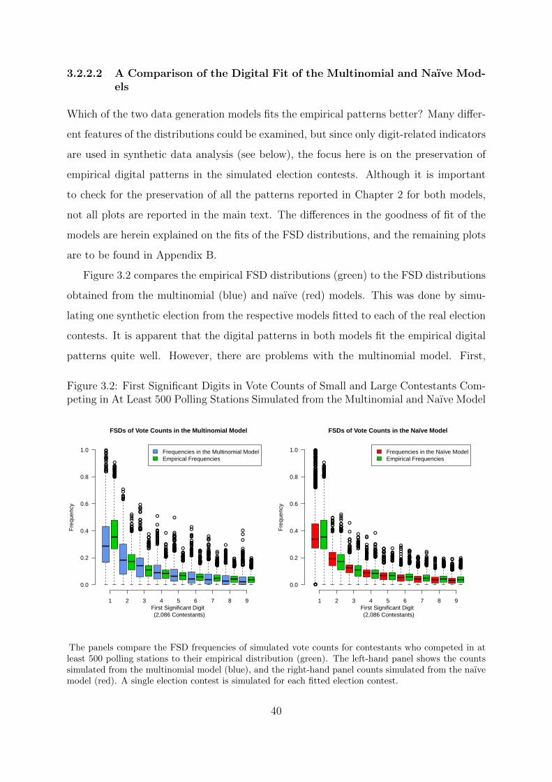
3.2.2.2 A Comparison of the Digital Fit of the Multinomial and Naıve Mod-els
Which of the two data generation models fits the empirical patterns better? Many differ-
ent features of the distributions could be examined, but since only digit-related indicators
are used in synthetic data analysis (see below), the focus here is on the preservation of
empirical digital patterns in the simulated election contests. Although it is important
to check for the preservation of all the patterns reported in Chapter 2 for both models,
not all plots are reported in the main text. The differences in the goodness of fit of the
models are herein explained on the fits of the FSD distributions, and the remaining plots
are to be found in Appendix B.
Figure 3.2 compares the empirical FSD distributions (green) to the FSD distributions
obtained from the multinomial (blue) and naıve (red) models. This was done by simu-
lating one synthetic election from the respective models fitted to each of the real election
contests. It is apparent that the digital patterns in both models fit the empirical digital
patterns quite well. However, there are problems with the multinomial model. First,
Figure 3.2: First Significant Digits in Vote Counts of Small and Large Contestants Com-peting in At Least 500 Polling Stations Simulated from the Multinomial and Naıve Model
●●●
●
●
●
●
●●●
●
●
●
●
●
●
●
●
●
●
●
●●●
●●●
●●
●
●●●●
●●●●●●
●●
●●
●
●●●
●●●●
●
●●●●●
●
●●●
●●
●●●●●
●●
●
●
●●
●●●●●●●
●●
●
●
●●
●
●●
●
●
●
●
●●
●
●●
●
●
●
●
●
●●
●●
●●●●●●
●●●●
●
●
●
●●●●
●
●
●●
●●●
●
●
●●
●
●●
●●●
●
●
●
●
●
●
●●●
●
●
●●●●●●●●
●●
●
●
●
●
●●
●●●●●●
●●
●●
●
●●●●●●
●
●
●●●
●
●
●●
●
●
●
●●●●
●
●●
●●
●●
●
●●
●
●
●●
●
●●●●
●●●●
●
●
●
●●
●●●
●
●●●●●●●
●●●
●●●●
●
●●
●
●
●
●
●
●●
●
●
●●
●
●●
●
●●●●
●●●
●
●●
●
●
●●
●
●
●●●
●●
●●●●
●●
●
●
●●●
●
●●●●
●●●
●●●●●●●
●●●
●
●
●
●●●
●●●●●
●
●
●
●
●
●●
●
●
●●●●●
●
●
●
●
●●
●
●
●
●
●●●
●●
●●
●
●
●
●●●●●
●
●●●●●●●●●●
●
●
●
●●
●
●
●●●●
●
●
●
●
●●●●
●●●●●●
●
●
●
●
●●●●
●
●
●●●
●●●●●
●●
●
●●
●
●●●
●●
●
●●
●
●
●●
●●●●●●●●
●●●●●
●
●●●●●●
●●●●
●●●●●●●●●●●●
●●●●●●
●●
●
●●●●
●
●
●
●
●●
●
●
●●
●
●
●
●●
●●●
●●●●●●●
●
●
●
●
●
●●
●●
●
●●●●●●●●●●●●
●●●
●●●●●●●●●
●●
●●●●●
●●
●●●●●●
●
●●
●●
FSDs of Vote Counts in the Multinomial Model
First Significant Digit (2,086 Contestants)
Fre
quen
cy
Frequencies in the Multinomial ModelEmpirical Frequencies
1 2 3 4 5 6 7 8 9
0.0
0.2
0.4
0.6
0.8
1.0
●
●
●
●●
●
●●
●
●
●●
●
●
●●
●●
●●
●
●
●●
●●
●
●
●
●
●
●
●
●
●
●
●
●
●●●
●
●●
●
●
●
●
●
●
●
●
●
●●●
●
●
●
●
●
●●
●
●●
●
●
●
●
●
●
●
●
●
●●
●
●
●●
●
●
●
●●●
●
●●●●
●
●●●
●
●●
●
●
●●
●
●
●
●●
●●●
●
●●●●
●●
●
●●●●
●●●●●●
●●
●●
●
●●●
●●●●
●
●●●●●
●
●●●
●
●
●●
●
●●●
●
●
●●
●
●●
●
●
●●
●●●●●●●
●●
●
●
●
●●●
●
●
●●●●●
●●●●●
●
●●
●
●
●
●
●
●●●●●●
●
●●●
●●
●●●●●●
●●●●
●
●
●
●●●●
●
● ●
●●●●
●●
●●
●
●●●●●
●
●
●
●
●●
●
●●●●
●
●●●
●●● ●●
●●●●●●
●●
●
●
●
●
●●
●●●●●●
●●
●●
●
●●●●●●
●●●●●●●●●●●●
●
●
●●●●
●●
●
●●●
●
●
●●
●●●
●
●
●●
●●
●●●
●
●●●●●●●
●●●
●●●●
●●●●●●●●●●●●
●●●●●●
●
●●●●
●●
●●
●●
●●●●
●
●●●
●
●
●●●
●
●●●●
●●●
●●●●●●●
●●●
●
●
●
●●●
●●●●●
●
●
●
●●
●
●●
●
●●●●
●
●
●●
●
●
●
● ●●●●●
●
●●●●●●●●●●
●
●
●
●●
●
●
●●●●
●
●
●
●
●●●●
●
●●
●
●●
●
●●
●
●●
●
●●
●
●●●●
●
●
●●●●●●●●●●●●
●●●●●
●
●●●●●●
●●●●
●●●●●●●●●●●●
●●●●●●
●●●●●●●
●
●●
●
●●●●●●
●●●●
●
●
●●
●●●●●●●●●● ●●
●●●●●●●●●
●●●
●●●●●●●●●
●●
●●●●●
●●
●●●●●●
●
●●
●●
FSDs of Vote Counts in the Naïve Model
First Significant Digit (2,086 Contestants)
Fre
quen
cy
Frequencies in the Naïve ModelEmpirical Frequencies
1 2 3 4 5 6 7 8 9
0.0
0.2
0.4
0.6
0.8
1.0
The panels compare the FSD frequencies of simulated vote counts for contestants who competed in atleast 500 polling stations to their empirical distribution (green). The left-hand panel shows the countssimulated from the multinomial model (blue), and the right-hand panel counts simulated from the naıvemodel (red). A single election contest is simulated for each fitted election contest.
40
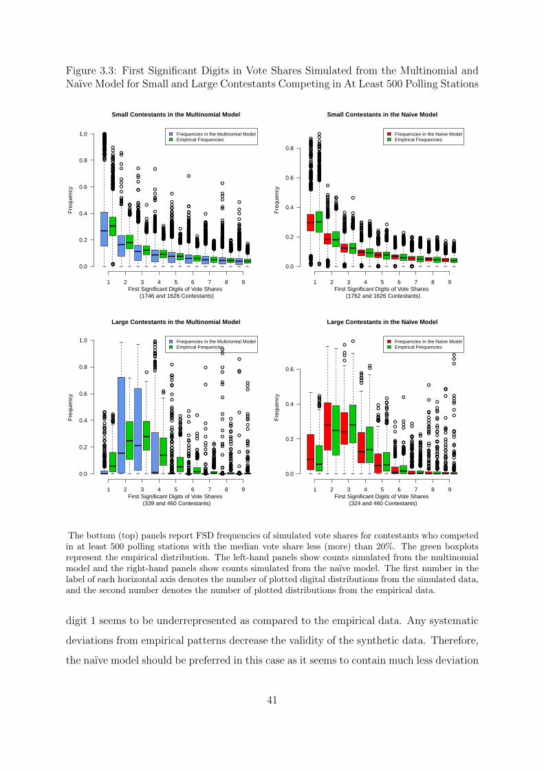
Figure 3.3: First Significant Digits in Vote Shares Simulated from the Multinomial andNaıve Model for Small and Large Contestants Competing in At Least 500 Polling Stations
●●●●●●
●
●
●●●
●●
●●●●●●
●
●
●
●●
●
●●
●
●
●
●●
●●●●
●
●
●●
●●●●●
●●
●●●●●●
●
●●
●
●●
●
●
●
●●●
●
●
●
●
●
●
●
●
●
●
●
●
●
●
●
●
●●●●
●
●
●
●
●
●●
●●
●
●
●
●●
●
●
●
●●●
●
●
●●●●
●
●●
●
●
●
●
●
●
●●
●
●●
●
●●
●
●
●
●
●
●●
●●
●●
●
●
●
●
●
●
●
●
●
●
●
●●●
●
●
●
●
●
●●
●●
●
●
●●
●
●
●
●
●
●
●
●
●
●●
●
●●
●
●●●
●
●
●
●
●
●
●
●●●●●
●
●
●
●●
●●●
●
●●●
●●●●●●●●●●●
●●●●●●●●
●●
●●
●
●
●
●●
●
●
●
●
●
●
●
●
●
●
●
●
●●●
●
●●●●●●●●●●
●●●●●●●●●
●●●●●
●●
●●●●
●
●●
●●●
●
●●●
●
●
●●●●●●●
●●●
●
●
●
●
●●●
●
●●●●●●●●
●
●●●●
●
●●●●●●●●●●
●●
●
●●●●
●●●●●●●●●●●
●●●
●●●●●●●
●
●●●
●●●●●
●
●
●●●
●●
●
●
●
●
●●●
●
●
●
●
●
●
●
●
●●
●
●
●●
●
●●●●
●●●●
●
●
●●●●
●
●●
●●●●
●●●
●
●
●
●
●●●●●●
●●
●
●●●●
●
●●
●
●●●
●
●●●●
●
●●●●
●●
●
●
●
●
●●●
●
●
●●●●
●●
●
●●
●●
●
●●●●●●
●●●●
●●●●●●
●
●●●
●●
●●
●●●●●●
●●●●●●●●●●●
●●●
●
●●●●●
●●●●
●
●
●
●
●●
●●
●●
●
●
●
●
●
●
●
●
●●●●●●●
●
●●
●
●●
●
●
●●
●
●
●
●●
●●●
●●
●●●
●
●
●●
●
●
●
●●●
●
●
●●●
●●
●●
●●
●●●●
●
●●
●●
●
●
●
●
●
●●
●
●●
●●●●●●●●●●●●●
●●
●
●
●●
●
●●●●
●●●●●●
●
●●●●●●●
●
●●●
●●●●●●●●
●
●
●
●
●
●●
●
●
●●
●
●
●
●
●
●
●●
●
●●
●
●
●●
●
●
●●●●
●●
●●●
●
●
●●
●
●
●
●
●
●●
●
●●
●
●
●
●
●
●●●●●
●
●
●
●●
●
●
●●●●●
●
●●
●
●
●
●
●●●
●●
●●
●●
●
●
●
●●
●
●
●
●●●
●
●
●
●
●
●
●
●
●
●
●
●
●●
●
●
●
●●●●●●●●●●●●●
●●●●●●●●●●●●●●●●
●
●
●●●●●
●●●●●●●●●●●●●
●●
●●●●●●●●●
●●●●●●●
●
●
●●
●
●●
●●
●●
●
●●
●
●●
●
●
●
●
●
●
●●
●
●
●
●
●
●
●
●
●
●●●●
●
●●
●
●●●●●
●●●●●●●●●
●
●
●
●
●●
●●
●●
●●●
●
●
●
●
●●●●
●●
●
●
●
●●
●●
●●●
●●
●
●
●
●
●●
●●●
●
●
●
●●●●●
●
●
●●●●
●●●●●●●●●
●●●●●●●
●
●●●●●
●●
●
●●●●●●●●●●●●●●●
●
●●●●●●●●●●●●
●
●
●
●●●●●●●●●
●●
●●
●
●●
●
●
●●
●
●
●
●
●
●●
●●
●
●●●●
●
●
●
●●
●
●
●●
●
●
●●
●
●
●
●
●●
●
●
●●●
●
●
●●
●
●●●
●
●●
●●●
●●●●●●
●
●●●●
●●
●
●
●
●●●●
●●●
●●
●●●●●●●●●
●
●●●●●●
●
●●
●
●
●
●
●●●●●●●●●●●●
●●●●●●●●●●●●●●●●
●●●●●
●●●●●●
●●
●●
●
●
●
●●●●●●●
●●●●
●●●●
●●●●●●●●
●● ●
●●
●●●●
●●●●●●●●
●●
●
●●
●●
●
●●
●
●●
●
●●●●●●●●
●●●●●
●
●
●
●
●
●
●
●●
●●
●
●
●
●●●
●
●●
●
●
●●●●●
●
●
●
●
●●●
●
●
●
●
●
●
●
●●●
●
●
●
●●
●
●●
●
●
●●●
●
●●●
●
●
●●●●●
●
●
●●
●●●●●●●●●●●●●●●●●●●●●●●●●●●
●
●●●●●●●●●●●●●
●
●●●●●●●
●
●●●●●●●●●
●●●●●●●●
Small Contestants in the Multinomial Model
First Significant Digits of Vote Shares (1746 and 1626 Contestants)
Fre
quen
cy
Frequencies in the Multinomial ModelEmpirical Frequencies
1 2 3 4 5 6 7 8 9
0.0
0.2
0.4
0.6
0.8
1.0
●
●
●●
●
●●
●●
●
●
●
●
●
●●
●
●
●
●●
●
●●
●●
●●
●
●●
●
●
●
●
●●
●
●
●
●
●
●
●
●
●
●
●
●●
●
●
●●
●
●
●
●●
●
●
●
●
●
●
●
●
●
●
●
●
●
●
●
●●
●
●●●
●
●
●
●
●●
●
●●
●
●
●
●
●
●
●
●
●
●
●●
●●●
●
●
●
●
●
●
●
●
●
●
●
●
●
●
●
●
●●
●●
●●
●
●●
●
●
●
●●
●
●
●
●●●
●
●
●
●●●
●
●●
●
●
●
●
●
●
●●
●
●●
●
●●
●
●
●
●
●
●●
●●
●●
●
●
●
●
●
●
●
●
●
●
●
●●●
●
●
●
●
●
●●
●●
●
●
●●
●
●
●
●
●
●
●
●
●
●●
●
●●
●
●
●●●●●●●
●●●●
●●●●
●●●
●●●
●●
●●●●●●●●
●●●●●●
●●
●●
●
●●
●
●
●
●●
●●●●●
●
●
●●
●
●●
●
●
●
●
●
●
●
●
●
●
●
●●●●●
●
●
●
●
●
●
●
●
●
●
●●●
●●●
●
●
●
●●●
●●●
●●
●
●
●
●●
●
●
●
●
●
●
●
●●●
●
●
●
●
●
●●●
●●●●
●
●
●
●
●
●●
●
●
●
●●
●
●
●
●
●●
●
●
●
●
●
●●●
●
●
●
●
●
●
●●
●●●
●
●●●
●●●●●●●●●●●
●●●
●●●●●●●●●●●●●
●
●●
●
●●●●●●●●●●●●●●●
●
●
●
●
●
●
●●
●
●
●
●●●●
●
●
●
●
●
●
●●
●
●●●
●
●
●
●
●
●●
●●
●
●
●
●●●
●
●●
●●●●●
●
●
●●
●
●●●●●●
●●
●●●
●
●
●●
●
●
●●● ●●
●
●
●●●●●●●●
●
●●●●
●
●●●●●●●●●●
●
●
●
●
●●●
●●●●●●●●●●●
●●●
●●●
●●●●
●
●
●●●●
●●
●
●
●●●
●
●●
●
●
●
●
●●
●
●●
●●
●
●●●●●●●●●●●●●●●
●
●●●●
●
●
●
●
●
●●
●
●●●
●●●
●
●●●
●
●
●
●●●
●
●
●●●
●●
●●●
●●
●
●●
●●
●●
●
●
●
●●●●
●
●●
●
●●
●●●
●
●
●
●
●
●●●
●
●
●
●●●
●●
●
●●
●●
●
●●●●●●
●●●●
●
●●●●●
●
●●●
●●
●
●
●●●●●●
●●●●●
●
●●●●●
●
●
●●
●
●●
●
●
●
●
●
●
●●●
●
●●●
●
●
●
●
●●
●●
●
●
●●
●●●●●●●●●●
●
●
●●●
●
●●●
●
●
●
●●
●
●
●●●●●●●●
●
●
●●
●
●●
●●●
●●
●●●
●
●●
●
●●●●●●
●●●
●
●●
●
●
●
●
●
●
●●●●
●●●●●●●●●
●●
●
●
●●
●
●●●●
●●●●●●
●
●●
●●●●●
●
●●●
●●●●●●●●
●
●
●●●
●●
●
●
●●●●●
●
●●●
●
●●●
●
●●●●●●●
●
●●●
●
●●
●●
●
●●
●●
●
●●●●●●●●●●
●●●
●●
●●
●
●●●
●
●
●●●
●
●●
●●●
●
●●
●
●●
●
●●●
●●●●●●●●●●●●●
●●●
●●●●●●●●●●●●●
●
●
●●●●●
●●●●●●●●●●●●●
●●
●●●●●●●●●
●
●●●
●
●●●
●●
●●●
●
●●
●
●●
●●●
●●●
●●●
●
●
●
●●●●
●●●●●●●●●●●●●
●
●●●●●
●
●●
●
●●
●●●●●●
●
●
●
●●●●
●●●
●
●
●
●
●
●●
●
●
●●●●
●
●
●
●●●
●
●
●
●
●●●●●●●●
●
●
●
●●●
●
●●●●●●●●●
●●●●●●●
●
●●●●●
●●
●
●
●●●●●●●●
●●●●●●
●
●●●●●●●●●●●●
●●●●
●●●●●●
●●●●●
●●●●●●●●●●●●●●●
●●●●●●●●●●●●●
●
●●
●
●
●
●●●●●●●●●●
●
●
●●
●
●●●
●
●
●
●●●●
●
●
●●●
●
●
●●●●●●●●●●●●
●
●●●●●●●●●●●●●●●
●
●●●
●
●●●●●●
●●
●●
●
●
●
●●●●●●●
●●●●
●●●
●
●●●●●●●●
●●
●●●●●●
●
●
●
●●
●
●●●●●●
●
●●
●●●●●
●
●●●●
●●●●●●●●●
●
●●
●
●●
●●●●●
●
●●
●
●
●●●
●●
●●●●●●●
●●●●●●
●
●
●●
●●●●●
●●●●●●●●●●●●●●●●●●●●●●
●
●●●●●●●●●●●●●
●
●●●●
●●
●
●
●●●●●●●●
●
●●●●●●●
●
Small Contestants in the Naïve Model
First Significant Digits of Vote Shares (1762 and 1626 Contestants)
Fre
quen
cy
Frequencies in the Naïve ModelEmpirical Frequencies
1 2 3 4 5 6 7 8 9
0.0
0.2
0.4
0.6
0.8
●●
●
●
●●●
●
●
●
●
●
●
●●
●●
●●
●
●●
●
●
●
●
●●
●●
●
●●
●
●
●
●
●
●●
●
●●
●
●●
●
●
●
●
●
●
●
●
●●●
●
●
●
●
●●●●●●●●
●
●
●
●
●
●
●
●●
●
●●
●
●
●
●
●●
●●
●●
●
●
●●
●
●
●
●
●●
●
●
●
●
●
●●
●●
●
●
●
●
●
●
●
●
●
●
●
●
●
●
●
●
●●
●
●
●
●
●
●
●
●
●●
●●●
●
●●
●
●
●
●
●
●
●
●
●
●
●
●
●
●
●
●
●
●
●
●
●
●
●
●
●
●
●
●●
●●
●●●
●●●
●●
●●
●
●
●●●●
●
●
●●●●●●●●●●●●●
●
●●●●
●
●●●●●●●●
●
●
●
●
●●
●
●
●
●●●●●●●●●
●
●
●
●●●●●●
●
●
●
●
●●
●
●
●●
●
●●●
●
●
●
●●
●
●
●●●
●●
●●●●●●
●
●●●●
●●●
●
●●●●●●●
●
●●●●●●●●
●
●
●●●●●●●●●
●
●●●●●●●●●●●●●●●●●●●●●●●●
●
●
●
●
●●●●●
●
●
●
●
●
●
●●
●
●
●●●●
●
●
●
●●
●●●●●●●
●
●●●●●●●●●●●●●●●●
●
●●
●
●
●
●
●●
●●
●
●
●
●
●
●
●
●●
●●●●
●
●
●
●
●●●●●●●●●●●●●●●●●●●●●●●●●●●●●●●
●
●
●
●
●●
●
●
●
●
●
●
●
●
●
●
●
●
●●
●
●●●●
●
●●●●●●●●●●●●●●
●●●
●
●
●●
●
●
●
●
●
●●
●
●
●
●●
●
●
●
●
●●
●
●
●
●
●●
●●●●●●●●●●●●●●●●●●●●●●●●●●●●●●●●●●●●●●●
●
●
●
●
●
●
●●●
●
●
●●●●●●
●
●●●●●●●●●●●●●●●●●●●●●●●●●●
●
●
●●
●
●
●●
●
●●
●
●
●
●
●
●
●
●
●
●
●
●
●
●●
●●
Large Contestants in the Multinomial Model
First Significant Digits of Vote Shares (339 and 460 Contestants)
Fre
quen
cy
Frequencies in the Multinomial ModelEmpirical Frequencies
1 2 3 4 5 6 7 8 9
0.0
0.2
0.4
0.6
0.8
1.0
●●●●●●●●
●
●
●
●
●
●●
●
●
●
●●●●●
●
●
●●
●
●
●●●
●
●●●●●
●●
●●
●
●●
●
●
●
●
●
●
●
●●●●
●
●
●
●
●
●
●●●●●●
●
●
●●●
●
●●●
●●●●●
●
●●●●●
●
●
●
●●
●
●
●●●●●●●
●●
●●●●●
●
●
●●●●
●●●
●
●●●●●●●
●
●●●●●●
●●
●
●
●
●●
●●●●
●
●
●
●●●●
●
●
●
●
●●
●
●
●●
●●●
●
●●
●
●
●
●
●
●
●
●
●
●●●●
●
●●
●
●
●
●
●
●●●●●●●
●
●
●●●●●●●●●●●●●●●
●
●●
●
●
●
●
●
●
●●
●
●
●
●
●
●
●
●●
●●●●
●
●
●
●
●●●●●●●●
●
●
●
●
●
●
●
●
●
●
●
●
●
●
●
●
●●●
●
●
●
●
●
●●
●
●
●●
●
●●
●●●●●●●●●●
●●
●●●
●
●
●●
●
●
●
●
●
●
●
●
●
●
●●
●
●
●
●
●●
●
●
●
●
●●
●
●
●●●●●●●●●●●
●
●
●
●
●●
●●
●
●
●
●
●●
●
●
●
●
●●
●
●
●
●
●●
●
●●●●●●●●●●●●●●●●●●●●●●●●●●
●
●
●●
●
●
●●
●
●●
●
●
●
●
●
●
●
●
●
●
●
●
●
●●
●●
Large Contestants in the Naïve Model
First Significant Digits of Vote Shares (324 and 460 Contestants)
Fre
quen
cy
Frequencies in the Naïve ModelEmpirical Frequencies
1 2 3 4 5 6 7 8 9
0.0
0.2
0.4
0.6
The bottom (top) panels report FSD frequencies of simulated vote shares for contestants who competedin at least 500 polling stations with the median vote share less (more) than 20%. The green boxplotsrepresent the empirical distribution. The left-hand panels show counts simulated from the multinomialmodel and the right-hand panels show counts simulated from the naıve model. The first number in thelabel of each horizontal axis denotes the number of plotted digital distributions from the simulated data,and the second number denotes the number of plotted distributions from the empirical data.
digit 1 seems to be underrepresented as compared to the empirical data. Any systematic
deviations from empirical patterns decrease the validity of the synthetic data. Therefore,
the naıve model should be preferred in this case as it seems to contain much less deviation
41
from the empirical FSD pattern. Moreover, the less flexible covariance structure of the
multinomial model (as compared to the naıve model) introduces more variance into the
data than exists in real election contests. On the other hand, the digital frequencies of
the naıve model reflect the empirical patterns very accurately.
Looking at vote share digital patterns yields even larger differences between the mod-
els. Similarly to the analysis in Chapter 2, Figure 3.3 divides the contestants into small
and large contestants using a boundary of a 20% median vote share. The top panels
relate to the small contestants, and the same patterns as in Figure 3.2 are visible: the
multinomial model produces significantly more variance and underrepresents low digits.
On the contrary, the naıve model is more precise. It is essentially unbiased and has only
slightly less variance than the empirical data. This is clearly visible when looking at the
vote share FSD distributions of large contestants (the bottom panels of Figure 3.3). The
multinomial model does not fit at all while the naıve model retains a good fit.
The better fit of the naıve model can be explained by the log-normal structure that it
inherits from the vote share model. As stated in Subsection 1.3.1, log-normal distributions
with sufficiently high variance (e.g. fitted vote share distributions of small contestants)
follow 1BL closely. The pattern of compliance with 1BL had also been identified for
empirical vote share distributions of small contestants (see Subsection 2.3.1).
To sum up, the naıve model fits the empirical data substantially better for some
patterns and comparably well for other patterns (see Appendix B for the remaining plots).
Because of this, simulations from this non-standard model will be used hereinafter.
3.2.3 Simulation Design and Fraud Imputation
After fitting the naıve model to each fraud-free electoral contest, 12,000 synthetic elec-
toral contests were simulated from every fitted model. Each simulated electoral contest
contained the same number of polling stations as the original contest. For instance, in
an election contest comprising 7 contestants in 2,241 polling stations, I started with a
2, 241× 7 table of vote counts. Next, the adjusted vote shares s′∗i were computed within
each polling station i, with i ∈ {1, 2, . . . , 2241}, and a linear regression model on the
simplex was fit to s′∗i with the vote total ti as a predictor (as in Equation 3.1).
42

The naıve model from Subsection 3.2.1 was then used to simulate vote counts in
new election contests. In the above example, each of the simulated contests would be
represented by a new 2, 241× 7 table of vote counts with the vote totals (approximately)
corresponding to ti in every polling station i. All together, 12,000 such tables were
simulated for each of the 5620 election contests in the dataset, summing up to a total of
67,440,000 simulated vote count tables (i.e., synthetic election contests).
The 12,000 simulated contests related to a single real election contest were further
divided into 8 groups of 1,500 tables each. The first group was left non-manipulated,
representing fraud-free contests. In the remaining 7 groups, different types/levels of
fraud were imputed based on a simple model of election fraud explained below.
While many models of fraud can be implemented, arguably the most intuitive one is
the one used by Cantu and Saiegh [2011]. Denoting as c1 the vote count of the contestant
benefiting from fraud and c2 the vote count of the contestant being harmed by it, they
computed fraudulent vote counts c∗1, c∗2 as follows:
c∗1 := c1 + bδγ · c2e,
c∗2 := b(1− γ) · c2e,
with b e representing rounding, γ ∈ [0, 1] denoting the proportion of c2 transferred to the
first candidate and δ ≥ 1 modelling ballot stuffing for the first candidate. Parameters γ
and δ are assumed to be constant across all polling stations.
The above model of fraud can easily be generalised for D contestants. Assuming that
only the strongest contestant (contestant 1) benefits from electoral manipulation (which
seems realistic as election fraud is typically implemented by the incumbent) their vote
counts are computed as follows:
c∗1 := c1 + bδγD∑j=2
cje,
c∗j := cj − uj, for j ∈ {2, . . . , D},
where uj represents the number of votes transferred from candidate j to candidate 1. If
43
U is a random variable that pools votes from contestants j ∈ {2, . . . , D} and samples
bγ∑D
j=2 cje of them, then uj is the number of sampled votes for contestant j. For example,
if in a polling station contestant 1 receives c1 = 40 true votes, and the remaining 3
contestants receive c2 = 10, c3 = 20 and c4 = 30 votes respectively and if γ = 0.5
and δ = 1.2, then the fraudulent vote count for the strongest candidate will be c∗1 =
40 + b1.2 · 0.5 · 60e = 76. Vote counts of the remaining candidates are determined by
pooling their 60 votes, randomly selecting b0.5 · 60e = 30 of them, determining which
candidates those votes belonged to, and then subtracting the given counts uj from the
true votes cj. If 3 votes of the second candidate, 11 votes of the third and 16 votes
of the fourth were randomly selected, then the fraudulent counts are c∗2 = 10 − 3 = 7,
c∗3 = 20− 11 = 9 and c∗4 = 30− 16 = 14 respectively.
In order to explore the model, different values of parameters γ and δ were used. Since
there is no a priori reason to believe that ballot stuffing and vote transferring occur to a
substantially different degree, the first five of the parameter value combinations were as
follows:
(γ, δ) ∈ {(0.01, 0.01), (0.05, 1.05), (0.1, 1.1), (0.3, 1.3), (0.5, 1.5)}
These parameter values define an ordinal structure of fraud levels : ranging from a small
amount of fraud (with 1% of votes transferred and 1% additional ballot stuffing) to an
extremely fraudulent election (with 50% of the votes transferred from their true candi-
dates to the incumbent and 50% more ballot-stuffing). The values are based on previous
research that suggested that the total percentage of fraudulent votes in an election con-
sidered as fraudulent by international standards could lie anywhere between 5 to 50%
[Cantu and Saiegh, 2011, Vorobyev, 2011, Enikolopov et al., 2012, Klimek et al., 2012].
The remaining two parameter combinations were aimed at determining whether the
fraud detection procedure can discriminate between different types of fraud. Therefore,
one was always selected to give a higher degree of fraud (50%) than the other (10%):
(γ, δ) ∈ {(0.1, 1.5), (0.5, 1.1)} .
From each of the 8 groups of 1,500 datasets, 1,000 were used to train a logistic learner
and 500 were used to test its performance.
44
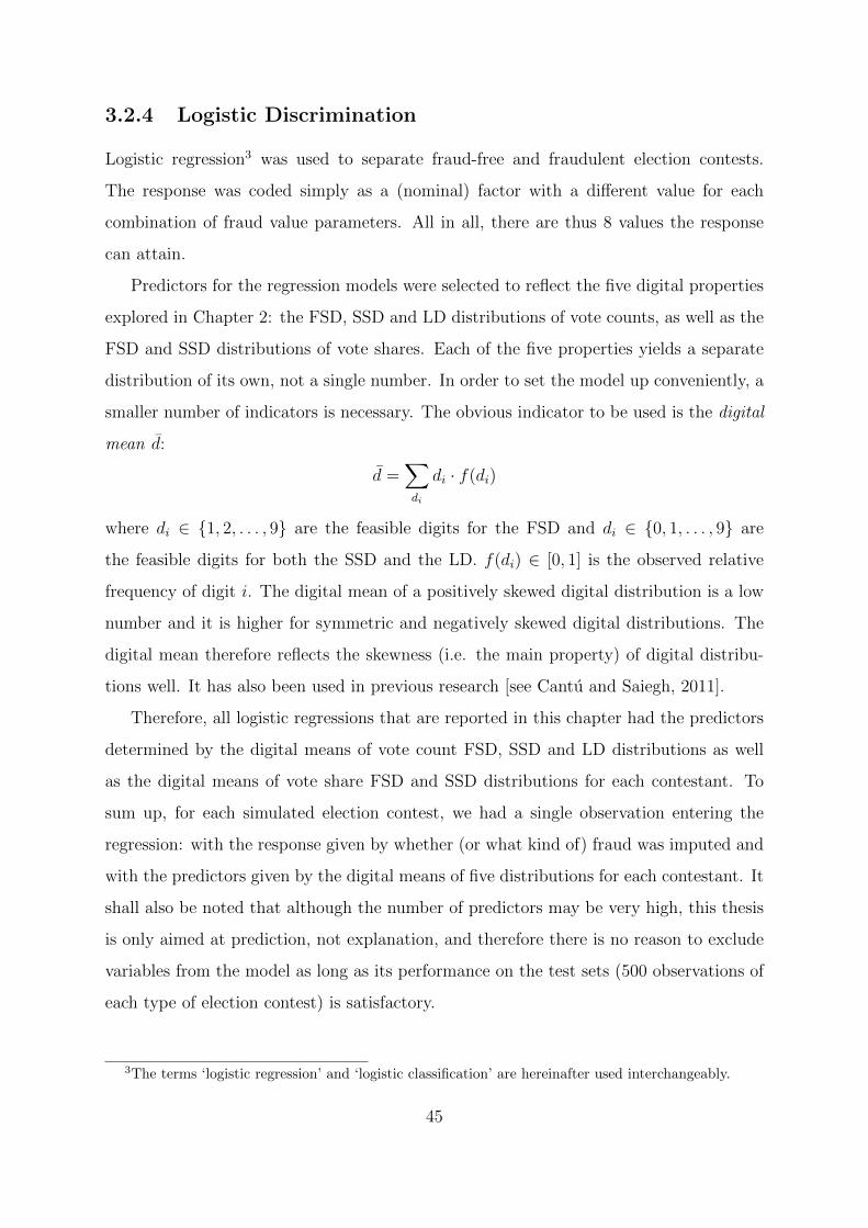
3.2.4 Logistic Discrimination
Logistic regression3 was used to separate fraud-free and fraudulent election contests.
The response was coded simply as a (nominal) factor with a different value for each
combination of fraud value parameters. All in all, there are thus 8 values the response
can attain.
Predictors for the regression models were selected to reflect the five digital properties
explored in Chapter 2: the FSD, SSD and LD distributions of vote counts, as well as the
FSD and SSD distributions of vote shares. Each of the five properties yields a separate
distribution of its own, not a single number. In order to set the model up conveniently, a
smaller number of indicators is necessary. The obvious indicator to be used is the digital
mean d:
d =∑di
di · f(di)
where di ∈ {1, 2, . . . , 9} are the feasible digits for the FSD and di ∈ {0, 1, . . . , 9} are
the feasible digits for both the SSD and the LD. f(di) ∈ [0, 1] is the observed relative
frequency of digit i. The digital mean of a positively skewed digital distribution is a low
number and it is higher for symmetric and negatively skewed digital distributions. The
digital mean therefore reflects the skewness (i.e. the main property) of digital distribu-
tions well. It has also been used in previous research [see Cantu and Saiegh, 2011].
Therefore, all logistic regressions that are reported in this chapter had the predictors
determined by the digital means of vote count FSD, SSD and LD distributions as well
as the digital means of vote share FSD and SSD distributions for each contestant. To
sum up, for each simulated election contest, we had a single observation entering the
regression: with the response given by whether (or what kind of) fraud was imputed and
with the predictors given by the digital means of five distributions for each contestant. It
shall also be noted that although the number of predictors may be very high, this thesis
is only aimed at prediction, not explanation, and therefore there is no reason to exclude
variables from the model as long as its performance on the test sets (500 observations of
each type of election contest) is satisfactory.
3The terms ‘logistic regression’ and ‘logistic classification’ are hereinafter used interchangeably.
45
3.3 Results
The results are presented in separate subsections. First, the fraud-free contests are merged
with the contests of each of the fraud types/levels separately and a binary logistic regres-
sion is used for classification. Subsection 3.3.2 then applies multinomial logistic regression
to discriminate between different fraud levels and Subsection 3.3.3 uses it to discriminate
between different fraud types. Moreover, both Subsection 3.3.2 and Subsection 3.3.3 look
at the importance of the digital means related to different digital patterns by using the
difference in deviances.
3.3.1 Separate Binary Logistic Regressions
First, different fraud levels were separately put into binary logistic regressions with the
fraud-free data. The models were fitted by maximum likelihood using function glm()
from R package stats. The main purpose of estimating these models is for visualising
the predictive performance of the logistic classifiers for different fraud levels using Re-
ceiver Operating Characteristic (ROC) curves. ROC curves plot sensitivity (estimated
probability of classifying a fraudulent election contest correctly) of a binary classifier
against its specificity (estimated probability of classifying a fraud-free election contest
correctly). Good classifiers should have both high sensitivity and specificity.
Figure 3.4 shows how the specificity and sensitivity of test set predictions depend on
the values of fraud parameters. Each of the four image plots represents a ‘cumulative’
plot of ROC curves for all 5,620 real empirical datasets. The dark blue regions show
rare specificity-sensitivity combinations and the red regions show the most commonly
occurring combinations. The ‘density’ of the regions is plotted on a log scale to simplify
visual interpretation of the plots.
The top-left panel of Figure 3.4 reports the ROC curves for the lowest fraud level
investigated (γ = 0.01, δ = 1.01). Prediction accuracy differs substantially between the
datasets. It is only slightly better than a coin toss for some election contests. On the
other hand, for most election contests it achieves perfect separation on the test set,
reaching the top-right corner of the plot. For the second-lowest fraud level (γ = 0.05, δ =
46
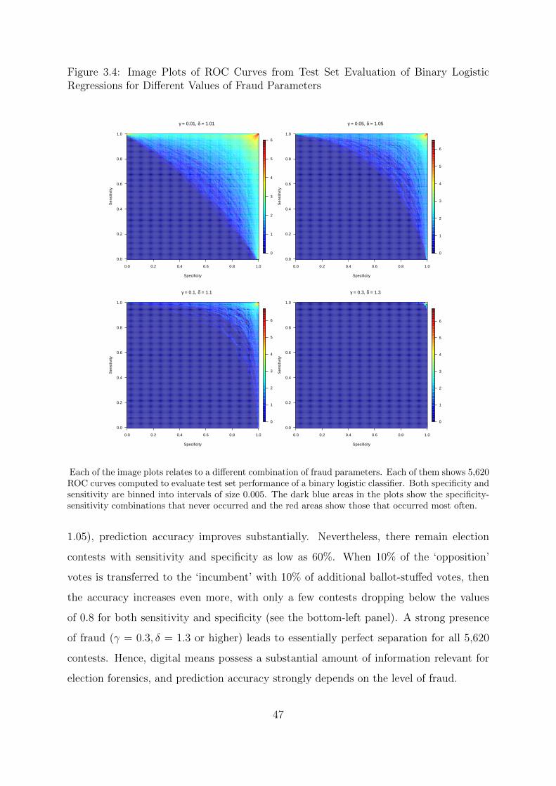
Figure 3.4: Image Plots of ROC Curves from Test Set Evaluation of Binary LogisticRegressions for Different Values of Fraud Parameters
0.0 0.2 0.4 0.6 0.8 1.0
0.0
0.2
0.4
0.6
0.8
1.0
Specificity
Sen
sitiv
ity
0
1
2
3
4
5
6
γ = 0.01, δ = 1.01
0.0 0.2 0.4 0.6 0.8 1.0
0.0
0.2
0.4
0.6
0.8
1.0
SpecificityS
ensi
tivity
0
1
2
3
4
5
6
γ = 0.05, δ = 1.05
0.0 0.2 0.4 0.6 0.8 1.0
0.0
0.2
0.4
0.6
0.8
1.0
Specificity
Sen
sitiv
ity
0
1
2
3
4
5
6
γ = 0.1, δ = 1.1
0.0 0.2 0.4 0.6 0.8 1.0
0.0
0.2
0.4
0.6
0.8
1.0
Specificity
Sen
sitiv
ity
0
1
2
3
4
5
6
γ = 0.3, δ = 1.3
Each of the image plots relates to a different combination of fraud parameters. Each of them shows 5,620ROC curves computed to evaluate test set performance of a binary logistic classifier. Both specificity andsensitivity are binned into intervals of size 0.005. The dark blue areas in the plots show the specificity-sensitivity combinations that never occurred and the red areas show those that occurred most often.
1.05), prediction accuracy improves substantially. Nevertheless, there remain election
contests with sensitivity and specificity as low as 60%. When 10% of the ‘opposition’
votes is transferred to the ‘incumbent’ with 10% of additional ballot-stuffed votes, then
the accuracy increases even more, with only a few contests dropping below the values
of 0.8 for both sensitivity and specificity (see the bottom-left panel). A strong presence
of fraud (γ = 0.3, δ = 1.3 or higher) leads to essentially perfect separation for all 5,620
contests. Hence, digital means possess a substantial amount of information relevant for
election forensics, and prediction accuracy strongly depends on the level of fraud.
47
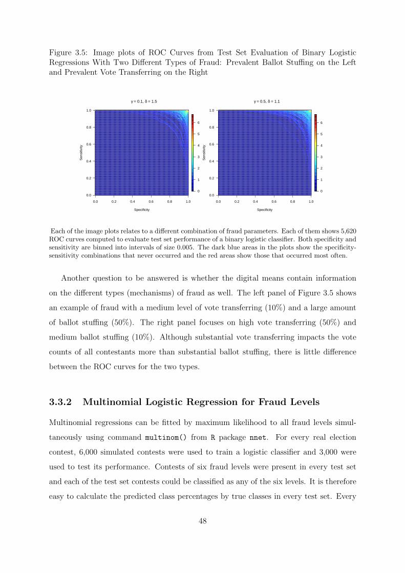
Figure 3.5: Image plots of ROC Curves from Test Set Evaluation of Binary LogisticRegressions With Two Different Types of Fraud: Prevalent Ballot Stuffing on the Leftand Prevalent Vote Transferring on the Right
0.0 0.2 0.4 0.6 0.8 1.0
0.0
0.2
0.4
0.6
0.8
1.0
Specificity
Sen
sitiv
ity
0
1
2
3
4
5
6
γ = 0.1, δ = 1.5
0.0 0.2 0.4 0.6 0.8 1.0
0.0
0.2
0.4
0.6
0.8
1.0
Specificity
Sen
sitiv
ity
0
1
2
3
4
5
6
γ = 0.5, δ = 1.1
Each of the image plots relates to a different combination of fraud parameters. Each of them shows 5,620ROC curves computed to evaluate test set performance of a binary logistic classifier. Both specificity andsensitivity are binned into intervals of size 0.005. The dark blue areas in the plots show the specificity-sensitivity combinations that never occurred and the red areas show those that occurred most often.
Another question to be answered is whether the digital means contain information
on the different types (mechanisms) of fraud as well. The left panel of Figure 3.5 shows
an example of fraud with a medium level of vote transferring (10%) and a large amount
of ballot stuffing (50%). The right panel focuses on high vote transferring (50%) and
medium ballot stuffing (10%). Although substantial vote transferring impacts the vote
counts of all contestants more than substantial ballot stuffing, there is little difference
between the ROC curves for the two types.
3.3.2 Multinomial Logistic Regression for Fraud Levels
Multinomial regressions can be fitted by maximum likelihood to all fraud levels simul-
taneously using command multinom() from R package nnet. For every real election
contest, 6,000 simulated contests were used to train a logistic classifier and 3,000 were
used to test its performance. Contests of six fraud levels were present in every test set
and each of the test set contests could be classified as any of the six levels. It is therefore
easy to calculate the predicted class percentages by true classes in every test set. Every
48
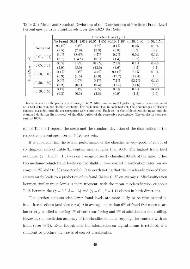
Table 3.1: Means and Standard Deviations of the Distributions of Predicted Fraud LevelPercentages by True Fraud Levels Over the 5,620 Test Sets
Predicted Class (γ, δ)No Fraud (0.01, 1.01) (0.05, 1.05) (0.10, 1.10) (0.30, 1.30) (0.50, 1.50)
Tru
eC
lass
(γ,δ
)
No Fraud93.1% 6.1% 0.6% 0.1% 0.0% 0.1%(9.5) (7.9) (2.3) (0.8) (0.2) (0.2)
(0.01, 1.01)6.4% 88.6% 4.7% 0.2% 0.0% 0.1%(8.7) (13.8) (6.7) (1.3) (0.2) (0.2)
(0.05, 1.05)0.8% 4.8% 91.6% 2.4% 0.1% 0.4%(2.9) (8.0) (13.0) (4.6) (0.3) (3.1)
(0.10, 1.10)0.1% 0.1% 2.4% 90.1% 7.1% 0.1%(0.9) (1.5) (5.0) (17.7) (17.4) (1.0)
(0.30, 1.30)0.0% 0.0% 0.1% 7.1% 92.7% 0.1%(0.2) (0.1) (0.3) (17.4) (17.6) (0.8)
(0.50, 1.50)0.1% 0.1% 0.3% 0.3% 0.4% 98.9%(0.3) (0.3) (2.8) (0.9) (1.3) (3.5)
This table assesses the prediction accuracy of 5,620 fitted multinomial logistic regressions, each evaluatedon a test sets of 3,000 election contests. For each true class in each test set, the percentages of electioncontests classified into the six categories were computed. Each cell of the table shows the mean and thestandard deviation (in brackets) of the distribution of the respective percentage. The entries in each rowsum to 100%.
cell of Table 3.1 reports the mean and the standard deviation of the distribution of the
respective percentages over all 5,620 test sets.
It is apparent that the overall performance of the classifier is very good. Five out of
six diagonal cells of Table 3.1 contain means higher than 90%. The highest fraud level
examined (γ = 0.5, δ = 1.5) was on average correctly classified 98.9% of the time. Other
two medium-to-high fraud levels yielded slightly lower correct classification rates (on av-
erage 92.7% and 90.1% respectively). It is worth noting that the misclassification of these
classes rarely leads to a prediction of no fraud (below 0.1% on average). Misclassification
between similar fraud levels is more frequent, with the mean misclassification of about
7.1% between the (γ = 0.3, δ = 1.3) and (γ = 0.1, δ = 1.1) classes in both directions.
The election contests with lower fraud levels are more likely to be misclassified as
fraud-free elections (and vice versa). On average, more than 6% of fraud-free contests are
incorrectly labelled as having 1% of vote transferring and 1% of additional ballot stuffing.
However, the prediction accuracy of the classifier remains very high for contests with no
fraud (over 93%). Even though only the information on digital means is retained, it is
sufficient to produce high rates of correct classification.
49
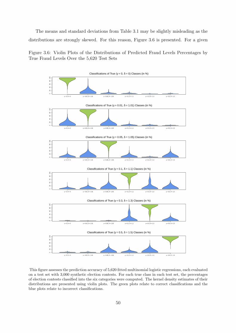
The means and standard deviations from Table 3.1 may be slightly misleading as the
distributions are strongly skewed. For this reason, Figure 3.6 is presented. For a given
Figure 3.6: Violin Plots of the Distributions of Predicted Fraud Levels Percentages byTrue Fraud Levels Over the 5,620 Test Sets
020
4060
8010
0
γ = 0, δ = 0 γ = 0.01, δ = 1.01 γ = 0.05, δ = 1.05 γ = 0.1, δ = 1.1 γ = 0.3, δ = 1.3 γ = 0.5, δ = 1.5
Classifications of True (γ = 0, δ = 0) Classes (in %)
020
4060
8010
0
γ = 0, δ = 0 γ = 0.01, δ = 1.01 γ = 0.05, δ = 1.05 γ = 0.1, δ = 1.1 γ = 0.3, δ = 1.3 γ = 0.5, δ = 1.5
Classifications of True (γ = 0.01, δ = 1.01) Classes (in %)
020
4060
8010
0
γ = 0, δ = 0 γ = 0.01, δ = 1.01 γ = 0.05, δ = 1.05 γ = 0.1, δ = 1.1 γ = 0.3, δ = 1.3 γ = 0.5, δ = 1.5
Classifications of True (γ = 0.05, δ = 1.05) Classes (in %)
020
4060
8010
0
γ = 0, δ = 0 γ = 0.01, δ = 1.01 γ = 0.05, δ = 1.05 γ = 0.1, δ = 1.1 γ = 0.3, δ = 1.3 γ = 0.5, δ = 1.5
Classifications of True (γ = 0.1, δ = 1.1) Classes (in %)
020
4060
8010
0
γ = 0, δ = 0 γ = 0.01, δ = 1.01 γ = 0.05, δ = 1.05 γ = 0.1, δ = 1.1 γ = 0.3, δ = 1.3 γ = 0.5, δ = 1.5
Classifications of True (γ = 0.3, δ = 1.3) Classes (in %)
020
4060
8010
0
γ = 0, δ = 0 γ = 0.01, δ = 1.01 γ = 0.05, δ = 1.05 γ = 0.1, δ = 1.1 γ = 0.3, δ = 1.3 γ = 0.5, δ = 1.5
Classifications of True (γ = 0.5, δ = 1.5) Classes (in %)
This figure assesses the prediction accuracy of 5,620 fitted multinomial logistic regressions, each evaluatedon a test set with 3,000 synthetic election contests. For each true class in each test set, the percentagesof election contests classified into the six categories were computed. The kernel density estimates of theirdistributions are presented using violin plots. The green plots relate to correct classifications and theblue plots relate to incorrect classifications.
50
true class it reports the distributions of predicted class percentages over all test sets.
The green violins show the distributions for the correct classifications and, as can be
seen, their distributions are in all cases strongly skewed towards the high values (close to
100%). On the contrary, the blue violins represent misclassification and they are always
skewed towards the small percentages.
Looking at the structure of the violin plots across the panels, it becomes clear that
the implemented parametrisation of fraud leads to a very symmetric misclassification
structure. Furthermore, distributions of the misclassification of the (γ = 0.3, δ = 1.3)
and (γ = 0.1, δ = 1.1) classes are bimodal. One mode is effectively at 0%, as expected,
but surprisingly a small mode around 50% appears as well. Last, while the category of
the largest fraud is rarely mistaken for the category of no fraud, it can be occasionally
misclassified as the (γ = 0.05, δ = 1.05) class.
Overall, the prediction accuracy of the multinomial classifier is high. It is natural to
ask whether or not all digital patterns provide useful information for correct classification
of election contests. A standard way of assessing the importance of a group of predictors
in multinomial regression is by the difference in the residual deviances of the full model
and a simpler model not containing the assessed predictors. For calculating the difference
in residual deviances, five more multinomial logistic models were fitted for each of the
5,620 datasets of simulated election contests (each of the five models fitted using the
digital means related to only four out of five digital patterns).
Aggregate results from applying the difference in deviance tests to all 5,620 datasets
for each pattern are reported in the left panel of Figure 3.7. For the sake of visualisation
simplicity, it plots the percentages of datasets with a p-value smaller than 0.01. All five
digital patterns yielded a smaller p-value for at least 60% of the datasets, showing that
all of them contain information that can often significantly reduce the deviance of the
fitted logistic model. However, some of the patterns seem to contain useful information
more often than other patterns. Most importantly, the FSDs for vote shares produce p-
values smaller than 0.01 for more than 99% of the datasets. These results seem reasonable
since digital means of vote share distributions are straightforwardly influenced by election
fraud (by introducing the pattern found in Section 2.4 and reported in the right panel
of Figure 2.10). Most importantly, the digital mean for the contestant benefiting from
51
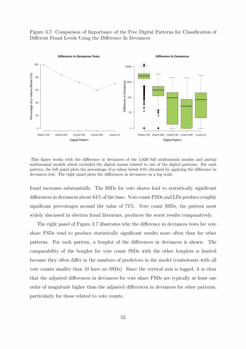
Figure 3.7: Comparison of Importance of the Five Digital Patterns for Classification ofDifferent Fraud Levels Using the Difference In Deviances
●
●
●
●
●
Difference in Deviances Tests
Digital Pattern
Per
cent
age
of p
−V
alue
s B
elow
0.0
1
0
20
40
60
80
100
Shares FSD Shares SSD Counts FSD Counts SSD Counts LD
●
●●
●
●●●●
●●
●●
●
●
●
●●
●
●
●
●
●
●
●●
●●
●
●
●
●
●
●
●
●●●●●●
●
●
●
●
●●●
●
●
●
●
●
●
●
●●
●●●
●
●
●
●
●
●
●
●
●●
●
●
●●●●●
●
●
●
●
●
●●
●
●●
●
●
●
●
●
●●●
●●
●●●
●
●
●
●
●●
●
●
●
●
●●●
●
●
●
●
●●
●●
●
●●
●
●
●
●
●
●
●
●●
●
●
●
●●
●●
●
●
●●
●
●
●
●●●
●
●
●●●●●●
●●●
●●
●
●●●
●
●
●
●●
●●
●
●●●
●
●●
●
●
●●●
●●
●●
●
●
●
●●
●
●
●●●
●
●
●
●
●
●
●
●
●
●
●
●
●
●●●
●
●
●●●●●
●●●
●
●
●
●
●
●
●
●
●
●
●
●
●
●
● ●●●●●●●●●●●●●●●●●●●●●●●●●●●●●●●●●●●●●●●●●●●●●●●●●●●●●●
●
●●●●●●●●●●●●●●●●●●●●●●●●●●●●●●●●●●●●●●●●●●●●●●●●●●●●●●●●●●●●●●●●●●●●●●●●●●●●●●●●●●●●●●●●●●●●●●●●●●●●●●●●●●●●●●●●●●●●●●●●●●●●●●●●●●●●●●●●●●●●●●●●●●●●●●●●●●●●●●●●●●●●●●●●●●●●●●●●●●●●●●●●●●●●●●●●●●●●●●●●●●●●●●●●●●●●●●●●●●●●●●●●●●●●●●●●●●●●●●●●●●●●●●●●●●●●●●●●●●●●●●●●●●●●●●●●●●●●●●●●●●●●●●●●●●●●●●●●●●●●●●●●●●●●●●●●●●●●●●●●●●●●●●●●●●●●●●●●●●●●●●●●●●●●●●●●●●●●●●●●●●●●●●●●●●●●●●●●●●●●●●●●●●●●●●●●●●●●●●●●●●●●●●●●●●●●●●●●●●●●●●
●
●●●●●●●●●●●●●●●●●●●●●●●●●●●●●●●●●●●●●●●●●●●●●●●●●●●●●●●●●●●●●●●●●●●●●●●●●●●●●●●●●●●●●●●●●●●●●●●●●●●●●
●
●●●●●●●●●●●●●●●●●●●●●●●●●●●●●●●●●●●●●●●●●●●●●●●●●●●●●●●●●●●●
●
●●●●●●●●●●●●●●●●●●●●●●●●●●●●●●●●●●●●●●●●●●●●●●●●●●●●●●●●●●●●●●●●●●●●●●●●●●●●●●●●●●●●●●●●●●●●●●●●●●●●●●●●●●
●
●●●●●●●●●●●●●●●●●●●●●●●●●●●●●●●●●●●●●●●●●●●●●●●●●●●●●●●●●●●●●●●●●●●●●●●●●●●●●●●●●●●●●●●●●●●●●●●●●●●●●●●●●●●●●●●●●●●●●●●●●●●●●●●●●●●●●●●●●●●●●●●●●●
●
●●●●●●
●
●●●
Difference In Deviances
Digital Pattern
Diff
eren
ce In
Dev
ianc
es0
10
100
1000
10000
Shares FSD Shares SSD Counts FSD Counts SSD Counts LD
This figure works with the difference in deviances of the 5,620 full multinomial models and partialmultinomial models which excluded the digital means related to one of the digital patterns. For eachpattern, the left panel plots the percentage of p-values below 0.01 obtained by applying the difference indeviances test. The right panel plots the differences in deviances on a log scale.
fraud increases substantially. The SSDs for vote shares lead to statistically significant
differences in deviances about 84% of the time. Vote count FSDs and LDs produce roughly
significant percentages around the value of 71%. Vote count SSDs, the pattern most
widely discussed in election fraud literature, produces the worst results comparatively.
The right panel of Figure 3.7 illustrates why the difference in deviances tests for vote
share FSDs tend to produce statistically significant results more often than for other
patterns. For each pattern, a boxplot of the differences in deviances is shown. The
comparability of the boxplot for vote count SSDs with the other boxplots is limited
because they often differ in the numbers of predictors in the model (contestants with all
vote counts smaller than 10 have no SSDs). Since the vertical axis is logged, it is clear
that the adjusted differences in deviances for vote share FSDs are typically at least one
order of magnitude higher than the adjusted differences in deviances for other patterns,
particularly for those related to vote counts.
52
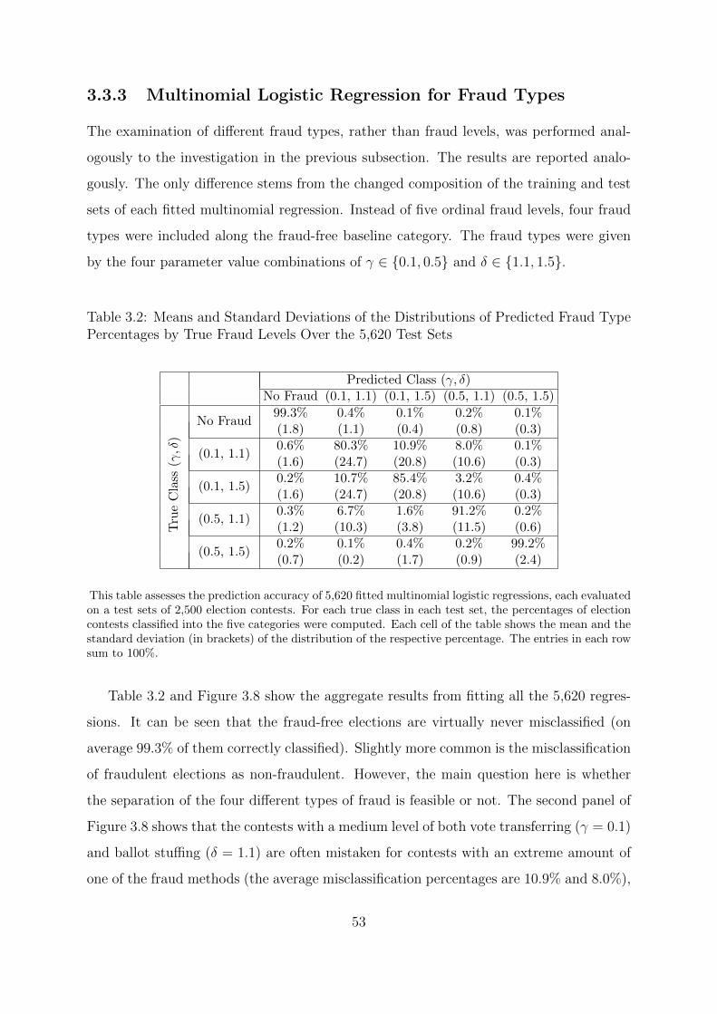
3.3.3 Multinomial Logistic Regression for Fraud Types
The examination of different fraud types, rather than fraud levels, was performed anal-
ogously to the investigation in the previous subsection. The results are reported analo-
gously. The only difference stems from the changed composition of the training and test
sets of each fitted multinomial regression. Instead of five ordinal fraud levels, four fraud
types were included along the fraud-free baseline category. The fraud types were given
by the four parameter value combinations of γ ∈ {0.1, 0.5} and δ ∈ {1.1, 1.5}.
Table 3.2: Means and Standard Deviations of the Distributions of Predicted Fraud TypePercentages by True Fraud Levels Over the 5,620 Test Sets
Predicted Class (γ, δ)No Fraud (0.1, 1.1) (0.1, 1.5) (0.5, 1.1) (0.5, 1.5)
Tru
eC
lass
(γ,δ
)
No Fraud99.3% 0.4% 0.1% 0.2% 0.1%(1.8) (1.1) (0.4) (0.8) (0.3)
(0.1, 1.1)0.6% 80.3% 10.9% 8.0% 0.1%(1.6) (24.7) (20.8) (10.6) (0.3)
(0.1, 1.5)0.2% 10.7% 85.4% 3.2% 0.4%(1.6) (24.7) (20.8) (10.6) (0.3)
(0.5, 1.1)0.3% 6.7% 1.6% 91.2% 0.2%(1.2) (10.3) (3.8) (11.5) (0.6)
(0.5, 1.5)0.2% 0.1% 0.4% 0.2% 99.2%(0.7) (0.2) (1.7) (0.9) (2.4)
This table assesses the prediction accuracy of 5,620 fitted multinomial logistic regressions, each evaluatedon a test sets of 2,500 election contests. For each true class in each test set, the percentages of electioncontests classified into the five categories were computed. Each cell of the table shows the mean and thestandard deviation (in brackets) of the distribution of the respective percentage. The entries in each rowsum to 100%.
Table 3.2 and Figure 3.8 show the aggregate results from fitting all the 5,620 regres-
sions. It can be seen that the fraud-free elections are virtually never misclassified (on
average 99.3% of them correctly classified). Slightly more common is the misclassification
of fraudulent elections as non-fraudulent. However, the main question here is whether
the separation of the four different types of fraud is feasible or not. The second panel of
Figure 3.8 shows that the contests with a medium level of both vote transferring (γ = 0.1)
and ballot stuffing (δ = 1.1) are often mistaken for contests with an extreme amount of
one of the fraud methods (the average misclassification percentages are 10.9% and 8.0%),
53
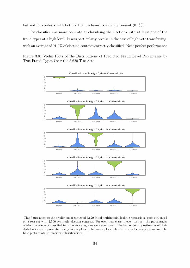
but not for contests with both of the mechanisms strongly present (0.1%).
The classifier was more accurate at classifying the elections with at least one of the
fraud types at a high level. It was particularly precise in the case of high vote transferring,
with an average of 91.2% of election contests correctly classified. Near perfect performance
Figure 3.8: Violin Plots of the Distributions of Predicted Fraud Level Percentages byTrue Fraud Types Over the 5,620 Test Sets
020
4060
8010
0
γ = 0, δ = 0 γ = 0.1, δ = 1.1 γ = 0.1, δ = 1.5 γ = 0.5, δ = 1.1 γ = 0.5, δ = 1.5
Classifications of True (γ = 0, δ = 0) Classes (in %)
020
4060
8010
0
γ = 0, δ = 0 γ = 0.1, δ = 1.1 γ = 0.1, δ = 1.5 γ = 0.5, δ = 1.1 γ = 0.5, δ = 1.5
Classifications of True (γ = 0.1, δ = 1.1) Classes (in %)
020
4060
8010
0
γ = 0, δ = 0 γ = 0.1, δ = 1.1 γ = 0.1, δ = 1.5 γ = 0.5, δ = 1.1 γ = 0.5, δ = 1.5
Classifications of True (γ = 0.1, δ = 1.5) Classes (in %)
020
4060
8010
0
γ = 0, δ = 0 γ = 0.1, δ = 1.1 γ = 0.1, δ = 1.5 γ = 0.5, δ = 1.1 γ = 0.5, δ = 1.5
Classifications of True (γ = 0.5, δ = 1.1) Classes (in %)
020
4060
8010
0
γ = 0, δ = 0 γ = 0.1, δ = 1.1 γ = 0.1, δ = 1.5 γ = 0.5, δ = 1.1 γ = 0.5, δ = 1.5
Classifications of True (γ = 0.5, δ = 1.5) Classes (in %)
This figure assesses the prediction accuracy of 5,620 fitted multinomial logistic regressions, each evaluatedon a test set with 2,500 synthetic election contests. For each true class in each test set, the percentagesof election contests classified into the six categories were computed. The kernel density estimates of theirdistributions are presented using violin plots. The green plots relate to correct classifications and theblue plots relate to incorrect classifications.
54
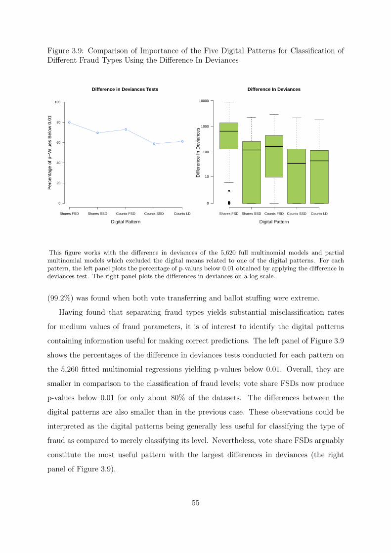
Figure 3.9: Comparison of Importance of the Five Digital Patterns for Classification ofDifferent Fraud Types Using the Difference In Deviances
●
●
●
●●
Difference in Deviances Tests
Digital Pattern
Per
cent
age
of p
−V
alue
s B
elow
0.0
1
0
20
40
60
80
100
Shares FSD Shares SSD Counts FSD Counts SSD Counts LD
●●●●●●●●●●●●●●●●●●●●●●●●●●●●●●●●●●●●●●●●●●●●●●●●●●●●●●●●●●●●●●●●●●●●●●●●●●●●●●●●●●●●●●●●●●●●●●●●●●●●●●●●●●●●●●●●●●●●●●●●●●●●●●●●●●●●●●●●●●●●●●●●●●●●●●●●●●●●●●●●●●●●●●●●●●●●●●●●●●●●●●●●●●●●●●●●●●●●●●●●●●●●●●●●●●●●●●●●●●●●●●●●●●●●●●●●●●●●●●●●●●●●●●●●●●●●●●●●●●●●●●●●●●●●●●●●●●●●●●●●●●●●●●●●●●●●●●●●●●●●●●●●●●●●●●●●●●●●●●●●●●●●●●●●●●●●●●●●●●●●●●●●●●●●●●●●●●●●●●●●●●●●●●●●●●●●●●●●●●●●●●●●●●●●●●●●●●●●●●●●●●●●●●●●●●●●●●●●●●●●●●●●●●●●●●●●●●●●●●●●●●●●●●●●●●●●●●●●●●●●●●●●●●●●●●●●●●●●●●●●●●●●●●●●●●●●●●●●●●●●●●●●●●●●●●●●●●●●●●●●●●●●●●●●●●●●●●●●●●●●●●●●●●●●●●●●●●●●●●●●●●●●●●●●●●●●●●●●●●●●●●●●●●●●●●●●●●●●●●●●●●●●●●●●●●●●●●●●●●●●●●●●●●●●●●●●●●●●●●●●●●●●●●●●●●●●●●●●●●●●●●●●●●●●●●●●●●●●●●●●●●●●●●●●●●●●●●●●●●●●●●●●●●●●●●●●●●●●●●●●●●●●●●●●●●●●●●●●●●●●●●●●●●●●●●●●●●●●●●●●●●●●●●●●●●●●●●●●●●●●
●
●●●●●●●●●●●●●●●●●●●●●●●●●●●●●●●●●●●●●●●●●●●●●●●●●●●●●●●●●●●●●●●●●●●●●●●●●●●●●●●●●●●●●●●●●●●●●●●●●●●●●●●●●●●●●●●●●●●●●●●●●●●●●●●●●●●●●●●●●●●●●●●●●●●●●●●●●●●●●●●●●●●●●●●●●●●●●●●●●●●●●●●●●●●●●●●●●●●●●●●●●●●●●●●●●●●●●●●●●●●●●●●●●●●●●●●●●●●●●●●●●●●●●●●●●●●●●●●●●●●●●●●●●●●●●●●●●●●●●●●●●●●●●●●●●●●●●●●●●●●●●●●●●●●●●●●●●●●●●●●●●●●●●●●●●●●●●●●●●●●●●●●●●
Difference In Deviances
Digital Pattern
Diff
eren
ce In
Dev
ianc
es0
10
100
1000
10000
Shares FSD Shares SSD Counts FSD Counts SSD Counts LD
This figure works with the difference in deviances of the 5,620 full multinomial models and partialmultinomial models which excluded the digital means related to one of the digital patterns. For eachpattern, the left panel plots the percentage of p-values below 0.01 obtained by applying the difference indeviances test. The right panel plots the differences in deviances on a log scale.
(99.2%) was found when both vote transferring and ballot stuffing were extreme.
Having found that separating fraud types yields substantial misclassification rates
for medium values of fraud parameters, it is of interest to identify the digital patterns
containing information useful for making correct predictions. The left panel of Figure 3.9
shows the percentages of the difference in deviances tests conducted for each pattern on
the 5,260 fitted multinomial regressions yielding p-values below 0.01. Overall, they are
smaller in comparison to the classification of fraud levels; vote share FSDs now produce
p-values below 0.01 for only about 80% of the datasets. The differences between the
digital patterns are also smaller than in the previous case. These observations could be
interpreted as the digital patterns being generally less useful for classifying the type of
fraud as compared to merely classifying its level. Nevertheless, vote share FSDs arguably
constitute the most useful pattern with the largest differences in deviances (the right
panel of Figure 3.9).
55
Conclusion
This thesis examined the potential and limits of digital election forensics by addressing
three main questions. First, are the digital patterns hypothesised in election forensics
literature present in fraud-free empirical data? Second, what other digital patterns exist
in fraud-free election results, and what models can we use to simulate election contests
similar enough to real-world data? Last, do digital patterns contain enough information
to accurately discriminate between fraud-free and fraudulent elections under the ideal
conditions of synthetic data analysis? By answering these three questions, the thesis
aimed to provide a complex assessment of the appropriateness of digital election forensics
both from an empirical and theoretical perspective. By doing so, it aimed to fill in the
gaps in the current academic discussion.
To tackle these questions, election results at the polling-station level were collected
from 5,630 election contests in 79 elections in 24 countries. A thorough examination of
the dataset revealed that the often assumed Benford’s law has at most limited empirical
validity for fraud-free election results; empirical distributions of the significant digits in
vote counts typically exhibit a stronger positive skew. This finding must be viewed in
light of the literature review in the first part of the thesis, which showed that the use of
Benford’s law was simply adopted from other fields where it had proven appropriate. On
the contrary, strong empirical support was found for the pattern of last digit uniformity in
vote counts of large contestants, a pattern that was articulated in the context of election
forensics.
In order to search for the actual empirical digital patterns in fraud-free election results,
vote shares were also explored. It was found that the digital patterns for vote shares are
no less present in the data than the patterns for vote counts. Furthermore, a commonly
occurring structure was identified in fraud-free vote share compositions: their distribution
56
tends to be close to a multivariate normal distribution on the simplex. Using this model
for fraud-free vote shares, I defined two models for fraud-free vote counts: the multinomial
model and the naıve model. Surprisingly, the naıve model outperformed the multinomial
model in the digital fit to empirical data, and was therefore chosen for simulating fraud-
free election contests.
As for the third question, thousands of artificial electoral contests were simulated from
each fraud-free election contest using the naıve model. Election fraud was then imputed
into a number of the simulated election contests. The datasets were used to train logistic
classifiers with the predictors given by the digital means for each contestant for each
pattern. The information contained in digital distributions was sufficient to allow for an
exceptionally accurate prediction of fraud level and a very accurate prediction of fraud
type. The most reduction in deviance was due to the first significant digit patterns in
vote shares.
The answers herein provided to all three of the questions above have their limitations.
Empirical exploration of digital patterns in election results should continue in the future.
More election data at the polling station level should be collected and the results should
be updated. Particularly scarce are results from fraudulent elections, and collecting more
of these results would allow for more straightforward research designs than the one imple-
mented in this dissertation. Also, more theoretical work needs to be done on modelling
multivariate election results, either non-parametrically or by defining a parametric fam-
ily more general than the family of normal distributions on the simplex. Finally, more
models of election fraud should be examined. One way of extending the model presented
here would be by incorporating random effects for the fraud parameters. Other plausible
fraud models also need investigation. All of these issues should be considered in future
research.
57
Bibliography
A. K. Adhikari. Some results on the distribution of the most significant digit. Sankhya:
The Indian Journal of Statistics, Series B (1960-2002), 31(3-4):413–420, 1969.
A. K. Adhikari and B. P. Sarkar. Distribution of most significant digit in certain functions
whose arguments are random variables. Sankhya: The Indian Journal of Statistics,
Series B (1960-2002), 30(1-2):47–58, 1968.
John Aitchison. The Statistical Analysis of Compositional Data. Chapman and Hall, New
York, 1986.
Bernd Beber and Alexandra Scacco. What the numbers say: A digit-based test for
election fraud. Political Analysis, 20(2):211–234, 2012.
Frank Benford. The law of anomalous numbers. Proceedings of the American Philosophical
Society, 78(4):551–572, 1938.
Sukanto Bhattacharya, Dongming Xu, and Kuldeep Kumar. An ANN-based auditor
decision support system using Benford’s law. Decision Support Systems, 50(3):576–
584, 2011.
Eric C. Bjornlund. Beyond Free and Fair: Monitoring Elections and Building Democracy.
Woodrow Wilson Center Press & Johns Hopkins University Press, 2004.
Jeff Boyle. An application of fourier series to the most significant digit problem. The
American Mathematical Monthly, 101(9):879–886, 1994.
Christian Breunig and Achim Goerres. Searching for electoral irregularities in an es-
tablished democracy: Applying Benford’s law tests to Bundestag elections in unified
Germany. Electoral Studies, 30(3):534–545, 2011.
58
Bruce Busta and Richard Sundheim. Tax return numbers tend to obey Benford’s law,
1992. URL http://bruceharvbusta.efoliomn.com/Workingpapers. Accessed on 27
August 2013.
Bruce Busta and Randy Weinberg. Using Benford’s law and neural networks as a review
procedure. Managerial Auditing Journal, 13(6):356–366, 1998.
Michael Callen and James D. Long. Institutional corruption and election fraud: Evidence
from a field experiment in Afghanistan, 2011. URL http://www.yale.edu/leitner/
resources/papers/em_eday_final.pdf. Accessed on 27 August 2013.
Francisco Cantu and Sebastian M. Saiegh. Fraudulent democracy? an analysis of ar-
gentina’s infamous decade using supervised machine learning. Political Analysis, 19
(4):409–433, 2011.
Charles A. P. N. Carslaw. Anomalies in income numbers: Evidence of goal oriented
behavior. The Accounting Review, 63(2):321–327, 1988.
The Carter Center. Observing the Venezuela presidential recall referendum: Comprehen-
sive report. Technical report, 2005. URL http://www.cartercenter.org/documents/
2020.pdf. Accessed on 27 August 2013.
Arnab Chatterjee, Marija Mitrovic, and Santo Fortunato. Universality in voting behavior:
An empirical analysis. Scientific Reports, 3, 2013.
Gary Cox. Making votes count: strategic coordination in the world’s electoral systems.
Cambridge University Press, Cambridge, 1997.
Joseph Deckert, Mikhail Myagkov, and Peter C. Ordeshook. Benford’s law and the
detection of election fraud. Political Analysis, 19(3):245–268, 2011.
Andreas Diekmann. Not the first digit! Using Benford’s law to detect fraudulent scientific
data. Journal of Applied Statistics, 34(3):321–329, 2007.
Stephan Dlugosz and Ulrich Muller-Funk. The value of the last digit: statistical fraud
detection with digit analysis. Advances in Data Analysis and Classification, 3(3):281–
290, 2009.
59
Maurice Duverger. Political Parties: Their Organization and Activity in the Modern
State. Methuen & Co., London, 1959.
Hans-Andreas Engel and Christoph Leuenberger. Benford’s law for exponential random
variables. Statistics & Probability Letters, 63:361–365, 2003.
Ruben Enikolopov, Vasily Korovkin, Maria Petrova, Konstantin Sonin, and Alexei Za-
kharov. Field experiment estimate of electoral fraud in russian parliamentary elections.
Proceedings of the National Academy of Sciences, 2012. URL http://www.pnas.org/
content/early/2012/12/19/1206770110. Accessed on 27 August 2013.
W. H. Furry and Henry Hurwitz. Distribution of numbers and distribution of significant
figures. Nature, 155(3924):52–53, 1945.
Marian Grendar, George Judge, and Laura Schechter. An empirical non-parametric like-
lihood family of data-based Benford-like distributions. Physica A, 380:429–438, 2007.
Joseph Hanlon and Sean Fox. Identifying fraud in democratic elections: A case study of
the 2004 presidential elections in Mozambique. 2006. URL http://eprints.lse.ac.
uk/41857/. Accessed on 27 August 2013.
J. A. Hartigan and P. M. Hartigan. The dip test of unimodality. The Annals of Statistics,
13(1):70–84, 1985.
T. P. Hill. The first digit phenomenon: A century-old observation about an unexpected
pattern in many numerical tables applies to the stock market, census statistics and
accounting data. American Scientist, 86(4):358–363, 1998.
Susan D. Hyde. How international election observers detect and deter fraud. In R. Michael
Alvarez, Thad E. Hall, and Susan D. Hyde, editors, Election Fraud: Detecting and
Deterring Electoral Manipulation, pages 201–215. Brookings Institution Press, 2008.
John E. Jackson. A seemingly unrelated regression model for analyzing multiparty elec-
tions. Political Analysis, 10(1):49–65, 2002.
Elise Janvresse and Thierry de la Rue. From uniform distributions to Benford’s law.
Journal of Applied Probability, 41(4):1203–1210, 2004.
60
Jonathan Katz and Gary King. A statistical model for multiparty electoral data. Amer-
ican Political Science Review, 93(1):15–32, 1999.
Peter Klimek, Yuri Yegorov, Rudolf Hanel, and Stefan Thurner. Statistical detection
of systematic election irregularities. Proceedings of the National Academy of Sciences,
109(41):16469–16473, 2012. URL http://www.pnas.org/content/109/41/16469. Ac-
cessed on 27 August 2013.
Lawrence M. Leemis, Bruce W. Schmeiser, and Diane L. Evans. Survival distributions
satisfying Benford’s law. The American Statistician, 54(4):236–241, 2000.
Ines Levin, Gabe A. Cohn, Peter C. Ordeshook, and R. Michael Alvarez. Detecting
voter fraud in an electronic voting context: an analysis of the unlimited reelection
vote in Venezuela. In Proceedings of the 2009 conference on Electronic voting technol-
ogy/workshop on trustworthy elections, Berkeley, 2009. USENIX Association. URL
http://dl.acm.org/citation.cfm?id=1855491.1855495. Accessed on 27 August
2013.
Drew A. Linzer. The relationship between seats and votes in multiparty systems. Political
Analysis, 20(3):400–416, 2012.
Rafael Lopez-Pintor. Assessing electoral fraud in new democracies: A basic con-
ceptual framework. In Whatever Happened to North-South?, Sao Paulo, 2011.
URL http://www.ifes.org/~/media/Files/Publications/White%20PaperReport/
2011/IPSA_conference_paper_pintor.pdf. Accessed on 27 August 2013.
Fletcher Lu and J. Efrim Boritz. Detecting fraud in health insurance data: Learning to
model incomplete Benford’s law distributions. In Joao Gama, Rui Camacho, Pavel B.
Brazdil, Alıpio Mario Jorge, and Luıs Torgo, editors, Machine Learning: ECML 2005,
number 3720 in Lecture Notes in Computer Science, pages 633–640. Springer Berlin
Heidelberg, 2005.
Fletcher Lu, J. Efrim Boritz, and Dominic Covvey. Adaptive fraud detection using Ben-
ford’s law. In Luc Lamontagne and Mario Marchand, editors, Advances in Artificial In-
61
telligence, number 4013 in Lecture Notes in Computer Science, pages 347–358. Springer
Berlin Heidelberg, 2006.
Walter R. Mebane, Jr. Election forensics: Vote counts and Benford’s law. UC-Davis, 2006.
URL http://analisis.elecciones2006.unam.mx/paperMebane.pdf. Accessed on
27 August 2013.
Walter R. Mebane, Jr. Election forensics: Statistics, recounts and fraud. Chicago, 2007.
URL http://www-personal.umich.edu/~wmebane/mw07.pdf. Accessed on 27 August
2013.
Walter R. Mebane, Jr. The second-digit Benford’s law test and recent American presiden-
tial election. In R. Michael Alvarez, Thad E. Hall, and Susan D. Hyde, editors, Election
Fraud: Detecting and Deterring Electoral Manipulation, pages 162–181. Brookings In-
stitution Press, 2008.
Walter R. Mebane, Jr. Election fraud or strategic voting? Can second-digit tests
tell the difference? Iowa, 2010a. URL http://polmeth.wustl.edu/media/Paper/
pm10mebane.pdf. Accessed on 27 August 2013.
Walter R. Mebane, Jr. Election fraud or strategic voting? Chicago, 2010b. URL
http://www-personal.umich.edu/~wmebane/mw10.pdf. Accessed on 27 August 2013.
Walter R. Mebane, Jr. A layman’s guide to statistical election forensics,
2010c. URL http://digest.electionguide.org/wp-content/uploads/2010/05/
mebane-19may2010.pdf. Accessed on 27 August 2013.
Walter R. Mebane, Jr. Comment on “Benford’s law and the detection of election fraud”.
Political Analysis, 19(3):269–272, 2011.
Walter R. Mebane, Jr. and Kirill Kalinin. Comparative election fraud detection. Chicago,
2009. URL http://www-personal.umich.edu/~wmebane/mw09png.pdf. Accessed on
27 August 2013.
Walter R. Mebane, Jr. and Jasjeet S. Sekhon. Robust estimation and outlier detection
62
for overdispersed multinomial models of count data. American Journal of Political
Science, 48(2):392–411, 2004.
John Morrow. Benford’s law, families of distributions and a test basis, 2010. URL
http://www.johnmorrow.info/projects/benford/benfordMain.pdf. Accessed on
27 August 2013.
James E. Mosimann and Makarand V. Ratnaparkhi. Uniform occurrence of digits for
folded and mixture distributions on finite intervals. Communications in Statistics -
Simulation and Computation, 25(2):481–506, 1996.
James E. Mosimann, Claire V. Wiseman, and Ruth E. Edelman. Data fabrication: Can
people generate random digits? Accountability in Research, 4:31–55, 1995.
Mikhail Myagkov, Peter Ordeshook, and Dimitry Shakin. Fraud or fairytales: Russia and
Ukraine’s electoral experience. Post-Soviet Affairs, 21(2):91–131, 2005.
Mikhail Myagkov, Peter Ordeshook, and Dmitry Shakin. The disappearance of fraud:
The forensics of Ukraine’s 2006 parliamentary elections. Post-Soviet Affairs, 23(3):
218–239, 2007.
Mikhail Myagkov, Peter C. Ordeshook, and Dimitry Shaikin. On the trail of fraud:
Estimating the flow of votes between russia’s elections. In R. Michael Alvarez, Thad E.
Hall, and Susan D. Hyde, editors, Election Fraud: Detecting and Deterring Electoral
Manipulation, pages 182–200. Brookings Institution Press, 2008.
Mikhail Myagkov, Peter C. Ordeshook, and Dimitri Shakin. The Forensics of Election
Fraud: Russia and Ukraine. Cambridge University Press, 2009.
Simon Newcomb. Note on the frequency of use of the different digits in natural numbers.
American Journal of Mathematics, 4(1):39–40, 1881.
Mark J. Nigrini. Digital analysis using Benford’s Law. Global Audit Publications, 2000.
Won-ho Park. Ecological inference and aggregate analysis of elections, 2008. URL http:
//deepblue.lib.umich.edu/handle/2027.42/58525. Accessed on 27 August 2013.
63
V. Pawlowsky-Glahn. Statistical modelling on coordinates. In Proceedings of the 1st
International Workshop on Compositional Data Analysis, Universitat de Girona, 2003.
URL http://ima.udg.es/Activitats/CoDaWork03. Accessed on 27 August 2013.
Luis Pericchi and David Torres. Quick anomaly detection by the Newcomb–Benford law,
with applications to electoral processes data from the USA, Puerto Rico and Venezuela.
Statistical Science, 26(4):502–516, 2011.
L. Pietronero, E. Tosatti, V. Tosatti, and A. Vespignani. Explaining the uneven dis-
tribution of numbers in nature: the laws of Benford and Zipf. Physica A: Statistical
Mechanics and its Applications, 293(1-2):297–304, 2001.
Ralph A. Raimi. The first digit problem. The American Mathematical Monthly, 83(7):
521–538, 1976.
R. J. Rodriguez. First significant digit patterns from mixtures of uniform distributions.
The American Statistician, 58:64–72, 2004.
P. Scott and M. Fasli. Benford’s law: An empirical investigation and a novel explanation.
Technical report, Department of Computer Science, University of Essex, 2001.
Steven W. Smith. The scientist and engineer’s guide to digital signal processing. California
Technical Pub., San Diego, 1997.
G. J. Szekely and M. L. Rizzo. A new test for multivariate normality. Journal of Multi-
variate Analysis, 93(1):58–80, 2008.
K. Gerald van den Boogaart and Raimon Tolosana-Delgado. Analyzing Compositional
Data with R. Springer, Heidelberg, 2013.
Dmitriy Vorobyev. Towards detecting and measuring ballot stuffing. SSRN eLibrary,
2011. URL http://papers.ssrn.com/sol3/papers.cfm?abstract_id=1965735. Ac-
cessed on 27 August 2013.
Wanda A. Wallace. Assessing the quality of data used for benchmarking and decision-
making. The Journal of Government Financial Management, 51(3):16–22, 2002.
64

Jonathan Wand, Jasjeet S. Sekhon, and Walter R. Mebane, Jr. A comparative anal-
ysis of multinomial voting irregularities: Canada 2000. Atlanta, 2001a. URL
http://elections.berkeley.edu/canada/multinom.canada.pdf. Not available on-
line anymore.
Jonathan N. Wand, Kenneth W. Shotts, Jasjeet S. Sekhon, Walter R. Mebane, Jr.,
Michael C. Herron, and Henry E. Brady. The butterfly did it: The aberrant vote
for Buchanan in Palm Beach County, Florida. American Political Science Review, 95
(04):793–810, 2001b.
65
Appendix A: Sources of Election
Results
Unless more specific information about the year or the type of an election is given, all
election results for the given country were compiled from the listed website or a reference.
All sources were accessible on 27 August 2013.
Afghanistan: Afghanistan Election Datahttp://afghanistanelectiondata.org/open/data
Armenia: Central Electoral Commissionhttp://www.elections.am/
Aruba: Electoral Councilhttp://www.gobierno.aw/
Bulgaria, European Parliament: Central Election Commissionhttp://ep2009.cik.bg/results/
Bulgaria, Lower House: Central Election Commissionhttp://pi2009.cik.bg/elected/
Canada: Elections Canadahttp://www.elections.ca/content.aspx?section=ele&lang=e
China (Hong Kong): Electoral Affairs Commissionhttp://www.eac.gov.hk/en/village/vre.htm
Curacao: Supreme Elections Councilhttp://www.kse.cw/index.html
Cyprus: The Ministry of Interiorhttp://www.proedrikes2013.gov.cy/index.htm
66
Czech Republic: Czech Statistical Officehttp://www.volby.cz/
Finland: Klimek et al. [2012]http://www.complex-systems.meduniwien.ac.at/elections/election.html
Germany: German Election Study (Princeton University)http://dss.princeton.edu/cgi-bin/catalog/search.cgi?studyno=3222
Jamaica: Electoral Commissionhttp://www.eoj.com.jm/content-183-179.htm
Mexico, 2009: Federal Electoral Institutehttp://prep2009.ife.org.mx/PREP2009/index prep2009.html
Mexico, 2012: Federal Electoral Institutehttps://prep2012.ife.org.mx/prep/NACIONAL/DiputadosNacionalVPP.html
Montenegro: State Electoral Commissionhttp://www.rik.co.me/
Nigeria: Beber and Scacco [2012]http://thedata.harvard.edu/dvn/dv/pan/faces/study/StudyPage.xhtml?globalId=hdl:1902.1/17151
Romania, 2009: Central Electoral Commissionhttp://www.bec2009p.ro/rezultateP.html
Romania, 2012: Central Electoral Commissionhttp://www.roaep.ro/istoric/
Russia: Klimek et al. [2012]http://www.complex-systems.meduniwien.ac.at/elections/election.html
Sierra Leone: National Electoral Commissionhttp://www.nec-sierraleone.org/
Sweden, 2002: Election Authorityhttp://thedata.harvard.edu/dvn/dv/pan/faces/study/StudyPage.xhtml?globalId=hdl:1902.1/17151
Sweden, 2006-2010: Election Authorityhttp://www.val.se/in english/previous elections/index.html
Uganda: Electoral Commissionhttp://www.ec.or.ug/eresults.php
67

United Kingdom (London): London Electshttp://www.londonelects.org.uk/im-voter/results-and-past-elections
Ukraine, 2004: Central Election Commissionhttp://www.cvk.gov.ua/pls/vp2004/WP0011
Ukraine, 2010: Central Election Commissionhttp://www.cvk.gov.ua/pls/vp2010/WP0011
United States (Chicago): Beber and Scacco [2012]http://dvn.iq.harvard.edu/dvn/dv/pan/faces/study/StudyPage.xhtml?globalId=hdl:1902.1/17151
68

Appendix B: Additional Plots
In order to make the figures easy to read, they are all printed on separate pages (starting
from the next page).
69
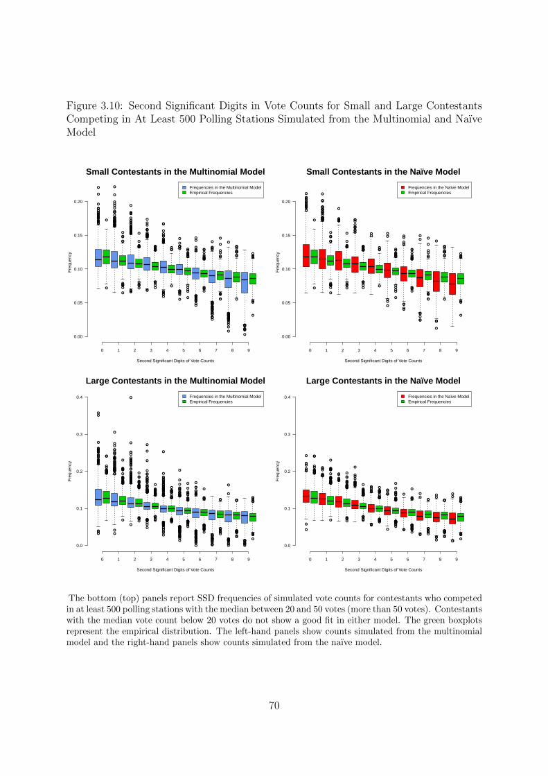
Figure 3.10: Second Significant Digits in Vote Counts for Small and Large ContestantsCompeting in At Least 500 Polling Stations Simulated from the Multinomial and NaıveModel
●
●
●
●
●
●●●
●●●
●
●●●
●
●●●
●●
●●●●
●
●
●
●
●
●
●
●
●
●
●●
●●
●
●
●
●
●
●
●●
●●
●
●
●
●
●
●
●●
●
●
●
●
●
●
●
●
●●
●
●●
●
●●
●
●
●
●
●
●
●
●
●
●
●
●
●
●
●
●
●
●
●
●●●●
●
●
●
●●
●
●
●●
●
●
●
●
●
●
●
●
●●
●●
●
●●●
●●●●
●
●
●●●●
●
●
●
●
●
●●●
●
●
●
●●
●
●●
●●
●●
●●●●●●
●
●●
●
●
●
●
●
●
●
●●●
●
●●
●
●
●
●
●
●
●● ●
●
●
●
●●
●●
●
●
●
●
●
●
●
●
●
●
●●●
●
●●
●
●
●
●
●
●
●
●
●●
●
●●●
●
●
●
●
●
●
●
●
●
●
●
●
●●
●●
●
●
●
●●●
●
●
●
●●
●
●●
●●
●
●
●
●
●
●●
●
●
●
●
●
●
●
●
●
●
●●
●
●
●
●
●
●
●
●
●
●●
●●
●
●
●
●
●
●●●
●●
●●
●
●
●
●●
●
●
●
●
●●●●●
●
●
●
●
●
●
●●●●
●
●
●
●
●
●
●
●
●
●
●●
●●
●●
●●
●
●
●
Small Contestants in the Multinomial Model
Second Significant Digits of Vote Counts
Fre
quen
cy
Frequencies in the Multinomial ModelEmpirical Frequencies
0 1 2 3 4 5 6 7 8 9
0.00
0.05
0.10
0.15
0.20●●
●
●
●
●
●
●●
●●
●
●
●●
●
●
●
●
●
●
●
●
●
●●
●
●
●●
●
●
●●●
●
●●●●
●●●
●
●
●●
●
●●
●
●●
●
●●
●
●
●
●●●●●●
●
●
●
●
●
●
●●
●●
●
●●●
●
●
●
●●
●
●
●●
●
●●
●
●●
●●
●●
●●●●●●
●●
●
●
●●
●
●
●
●
●
●
●
●
●
●
●●●
●
●●
●
●
●
●
●
●●
●
●●
●
●
●
●
●
●●
●●
●
●
●
●●●
●
●
●
●
●
●●
●
●
●
●
●
●●
●●
●
●
●
●
●
●
●
●●●
●
●
●
●
●●●●
●
●
●
●●
●●
●●
●
●
●
Small Contestants in the Naïve Model
Second Significant Digits of Vote Counts
Fre
quen
cy
Frequencies in the Naïve ModelEmpirical Frequencies
0 1 2 3 4 5 6 7 8 9
0.00
0.05
0.10
0.15
0.20
●
●●
●
●●●●●
●
●●
●
●●
●
●
●
●
●
●●●●
●
●●●
●
●●●●●●●
●●●
●
●
●
●●
●
●●
●
●●
●
●
●
●
●
●
●
●
●
●
●
●●
●
●●
●
●
●
●
●●●
●
●
●
●
●
●●
●
●●
●●●●●
●●
●
●
●
●
●
●
●
●
●●
●
●
●
●
●
●●●
●
●
●
●
●
●●●●
●
●
●●
●
●●
●
●
●
●●
●●
●
●
●
●
●
●
●●
●●
●
●
●
●
●
●
●
●
●
●
●
●
●
●●●●
●
●
●
●
●
●●
●
●
●
●
●
●
●●
●●
●●
●●
●
●
●
●
●
●
●
●
●●
●
●●
●
●
●●
●
●
●●
●●
●
●
●
●
●
●●●●
●
●
●
●
●
●
●
●
●●
●
●●●●●
●●
●●●●
●
●
●
●●●●
●
●
●
●●●●●
●
●
●
●
●
●
●
●
●●●
●●●
●●
●
●
●
●
●
●●
●
●
●
●
●●
●
●●●
●
●
●
●
●
●●
●
●
●
●
●
●
●
●
●
●
●
●
●●
●
●
●
●
●
●●
●
●
●
●●
●
●
●●
●
●●
●
●
●
●
●●
●●
●
●
●
●
●●
●
●●
●
●
●
●●●
●
●●
●
●
●
●
●●
●
●
●
●
●
●●
●
●
●
●
●
●
●
●
●
●
●●●
●
●
●
●
●
●
●
●●●
●
●●
●
●●
●●
●●
●●●
●
●
●●●
●
●
●
●
●
●
●
●
●
●
●
●
●●
●
●●
●
●
●
●
●
●●●
●
●
●
●●
●
●
●
●
●
●
●
●
●
●
●
●
●
●
●
●
●●●
●
●
●
●●
●●
●●
●
●
●
●
●
●
●
●
●
●●●●
●●●
●●●●●●●●
●
●●
●
●
●●●
●●●
●●●●
●
●●
●
●
●
●
●
●●
●●●
●
●●●●●
●●●
●
●●●●●●●●
●●
●●●
●●●●
●●
●●●
●●
●
●
●
Large Contestants in the Multinomial Model
Second Significant Digits of Vote Counts
Fre
quen
cy
Frequencies in the Multinomial ModelEmpirical Frequencies
0 1 2 3 4 5 6 7 8 9
0.0
0.1
0.2
0.3
0.4
●●
●●
●
●
●
●
●
●●●●●●●
●●●
●
●
●
●
●
●●●
●●●●●
●●●●●
●●
●
●
●
●
●
●
●
●
●●
●
●
●
●
●
●●●
●●
●●●●●●●
●
●
●
●
●
●
●
●
●
●●●●
●
●
●
●
●
●●
●
●
●
●
●
●
●●
●
●●
●●●●●●●●
●
●●
●●●
●●
●●●●
●
●
●
●●●●
●
●
●
●●●●●
●
●
●
●●
●
●
●●
●
●●
● ●
●●
●
●
●●
●
●●
●
●
●
●
●●
●●
●
●
●
●
●●
●
●●
●
●● ●●
●
●●
●●
●●
●●●
●
●
●●●
●
●
●
●
●
●
●
●
●
●
●
●
●●
●
●
●
●
●●
●●
●●
●
●
●
●
●
●
●
●
●
●●●●
●●
●
●
●
●●●●
●
●●
●
●
●
●●
●●●
●●●
●
●●●●●●●●
●
●●
●
●●
●●●
●●
●
●
●
Large Contestants in the Naïve Model
Second Significant Digits of Vote Counts
Fre
quen
cy
Frequencies in the Naïve ModelEmpirical Frequencies
0 1 2 3 4 5 6 7 8 9
0.0
0.1
0.2
0.3
0.4
The bottom (top) panels report SSD frequencies of simulated vote counts for contestants who competedin at least 500 polling stations with the median between 20 and 50 votes (more than 50 votes). Contestantswith the median vote count below 20 votes do not show a good fit in either model. The green boxplotsrepresent the empirical distribution. The left-hand panels show counts simulated from the multinomialmodel and the right-hand panels show counts simulated from the naıve model.
70
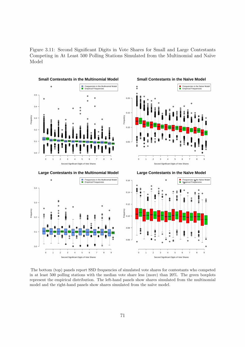
Figure 3.11: Second Significant Digits in Vote Shares for Small and Large ContestantsCompeting in At Least 500 Polling Stations Simulated from the Multinomial and NaıveModel
●
●
●
●
●
●
●
●
●
●●●
●
●
●●●
●●●
●●
●
●●
●●
●
●
●
●
●
●
●●
●
●
●
●
●
●
●
●
●
●
●
●
●
●
●
●
●
●●●
●
●
●
●
●
●
●
●
●
●
●
●●
●
●
●
●
●●
●
●
●
●●
●
●
●
●●●
●
●
●
●
●
●
●
●
●
●
●●
●
●●●
●
●
●
●
●●●
●
●
●●
●
●
●
●
●
●
●●
●
●
●
●
●
●
●
●
●
●
●
●
●
●●
●●
●
●
●
●●
●●
●
●
●
●
●
●
●●●
●
●
●●
●
●
●●
●
●
●
●
●
●
●
●
●
●
●
●
●
●●
●
●●
●
●
●
●
●●
●
●●
●
●
●
●
●●
●●●●
●
●●●
●
●●●●
●●●●
●●
●
●
●
●
●
●●
●●●
●●●
●
●●●●●
●
●
●●
●●●
●
●
●
●●
●●●
●
●●●●●●
●
●●
●
●
●●
●
●
●●
●
●
●●
●
●●
●
●
●
●●
●●●●●
●
●
●
●
●
●
●
●
●●
●
●
●
●
●
●●
●
●
●
●
●
●
●
●
●
●●
●
●
●
●
●
●
●
●
●
●
●
●
●
●●●
●
●
●
●
●
●
●
●
●
●
●
●
●●
●●
●
●
●
●
●
●
●
●
●●
●
●
●
●●●
●
●●
●●
●
●
●
●
●
●●●●
●
●
●
●
●
●
●
●
●
●
●
●●
●●
●●
●
●●
●
●
●
●
●
●
●
●
●
●
●
●
●
●
●
●
●●
●●
●
●
●
●●
●
●
●●
●
●
●●
●●
●
●
●
●
●
●
●●●●
●
●
●●
●
●
●
●
●●●
●
●●
●●
●
●●●●
●
●●
●●
●
●
●
●●●●
●
●●●
●
●●
●●●●
●●
●
●
●
●●●
●
●●●
●
●
●
●
●
●
●
●
●●●
●
●●●
●
●
●
●
●●●●●●
●
●
●
●
●
●
●●
●
●
●●
●●
●
●●
●
●●●
●
●
●
●
●
●
●●
●
●
●
●
●
●●
●
●
●●
●
●
●
●
●
●
●
●
●
●●●
●
●
●
●
●
●
●
●
●●
●
●●
●●
●
●
●
●●●●
●
●
●
●
●●
●
●●●
●
●
●
●
●
●●
●
●
●
●
●
●
●
●
●
●
●
●
●
●
●
●●●
●
●
●●
●
●
●●
●
●
●
●
●
●
●
●●
●●
●●
●●●
●
●
●
●●
●
●●
●
●
●
●
●●●●●
●●●
●
●●
●
●
●
●
●
●●
●
●
●
●
●
●
●●
●
●
●●
●
●
●
●
●
●
●●●●●●●●●●●●●
●
●
●●
●●●●●
●●
●
●●
●
●
●
●
●
●
●●
●●●
●●
●
●
●●●●
●●
●
●
●●
●
●●●
●
●●
●
●
●
●
●
●
●●
●●
●
●
●
●
●●
●
●
●
●
●●
●
●
●
●●●●●
●
●
●
●
●
●●
●
●
●
●
●●
●
●
●
●●
●
●●
●
●
●
●
●
●
●
●
●
●●
●
●
●
●
●
●
●
●
●
●
●
●
●
●●●●
●
●
●
●
●●
●
●
●
●●
●●●●●
●
●
●●
●
●●
●
●
●●
●
●
●
●
●
●
●
●
●●
●
●
●
●
●
●
●
●
●
●●
●
●
●
●●●●
●
●
●
●
●●
●●
●
●
●
●
●
●●●
●●
●
●
●
●
●
●
●●
●
●
●
●
●●●
●
●
●●
●●
●
●
●
●
●
●
●
●
●●
●
●●
●
●
●
●
●●
●●●●●●●
●●
●●●●●●●●●
●●
●
●●
●●●
●
●
●
●●
●
●
●●●
●
●
●●●
●●●●
●●●●●●●
●●●●
●●●●●
●●
●●
●
●●●●
●●●
●
●
●
●
●●
●
●
●
●●
●
●
●
●
●
●●
●●
●
●
●
●
●
●
●
●
●
●
●
●
●
●
●
●
●●
●
●
●
●
●
●●
●
●
●
●
●
●
●
●
●●
●
●●●●●●
●
●●
●●
●●
●
●
●
●
●
●
●
●
●
●
●
●
●
●
●
●●
●
●
●●
●
●
●
●
●●
●
●
●
●
●
●
●
●
●
●●
●
●
●●
●
●
●●●●●
●●●●
●
●●
●
●●●
●
●
●●
●
●
●
●
●
●
●
●
●
●
●
●
●
●●●
●●
●
●
●
●
●●●
●
●
●
●●
●
●
●
●
●●●●●●●
●
●
●
●
●
●
●
●●
●
●
●●
●
●●
●
●●●●
●
●●
●
●
●●
●●●
●●●●●
●
●
●●●
●●●
●
●
●●●
●●●●●
●●●
●●
●
●
●
●
●●
●
●
●●
●●
●●
●
●
●
●
●
●
●
●
●
●
●
●
●
●
●●
●
●●
●
●
●●
●
●
●
●
●
●
●
●●●
●
●
●
●
●
●
●
●
●
●
●
●
●
●
●
●
●
●
●
●
●
●
●
●
●
●
●●●●
●
●
●●●●
●
●●
●●
●
●
●●
●
●
●●
●●
●●
●
●
●
●●●●●
●
●●
●
●
●
●
●
●
●
●
●
●
●
●
●●
●
●
●●
●
●
●
●●
●
●●
●
●
●
●
●
●
●
●●
●
●
●●
●●●
●
●
●●
●
●
●
●
●
●
●●
●
●
●
●
●
●
●●
●
●
●
●
●
●
●
●
●
●
●●●●
●
●●
●●●
●
●
●●
●●
●
●
●
●●●
●●●
●
●
●
●
●●●●●●
●
●
●
●
●
●
●●
●
●●●
●●
●
●
●
●
●
●
●●●
●
●
●
●●
●
●
●
●●●
●
●
●●
●
●
●
●
●●
●
●
●
●
●
●
●
●
●
●
●
●
●
●
●
●
●
●
●
●
●●
●
●
●
●
●
●
●
●
●
●
●●●
●
●
●
●
●
●
●●
●
●●●
●
●●
●
●
●
●
●
●
●
●
●
●
●
●●●●
●●
●
●
●●
●
●
●●●
●
●
●
●●●
●
●
●
●
●
●●
●●●
●
●
●
●
●
●
●
●●●
●
●
●●
●●
●●
●●
●
●
●
●
●
●
●
●
●●
●
●●
●●
●
●●●
●
●●
●●
●
●●●●
●
●
●
●
●●
●
●●
●
●
●●
●●
●
●
●
●●●
●
●
●
●●
●●
●●
●
●●●
●●●
●●●
●
●●
●
●
●
●
●
●
●
●●●
●
●
●●●
●●
●
●●
●
●
●●
●
●
●
●
●
●
●
●
●●●
●
●●●
●
●●
●
●
●●
●
●●
●
●
●
●
●
●
●
●
●
●
●
●
●
●
●
●
●
●●●●
●
●
●
●
●
●
●
●
●
●
●
●
●
●
●
●
●
●
●●●
●●●
●
●
●
●
●
●●●●
●
●●●●
●
●
●
●
●●●
●
●
●●
●●●
●●
●
●
●
●
●●
●
●
●●
●●
●
●
●●
●●
●
●
●●●
●
●●●●
●●●●
●
●
●
●
●
●
●
●
●
●
●
●
●
●
●
●●
●
●
●
●
●●
●
●●●
●●●●●
●
●●●●●●
●●
●●
●
●●
●●
●●
●
●
●
●
●●
●●●●
●
●●
●●
●
●●●●
●
●●
●
●●
●●●
●
●
●
●
●
●
●●●
●●
●●
●●●●●●●●
●●●
●
●
●
●
●●
●
●
●
●
●
●●
●●
●
●●
●
●●●●●●●
●
●●
●
●
●●
●
●●
●
●
●
●●●
●
●●
●●
●
●●
●
●●
●●●
●
●
●
●
●
●
●●
●
●
●●
●
●
●
●
●
●●●
●
●
●
●●
●
●
●
●
●
●●
●
●
●
●
●●●●
●●
●
●
●●
●
●
●
●
●
●●
●●●●
●
●●
●
●
●●●
●
●●●●●●
●
●
●●
●●●
●
●
●
●
●
●●
●
●
●
●
●
●
●●●
●
●●●●●●●●
●
●●●●●
●●
●●
●
●●
●
●
●●●●
●●
●●●●●●
●●
●●
●●
●
●
●
●
●
●
●
●
●●●●
●
●
●
●
●
●
●●
●
●
●●
●
●
●●●
●
●●●
●
●
●●●●●●●
●●
●●
●●●
●
●
●●●●●
●
●
●
●
●
●●
●●●●●
●
●
●
●
●
●
●●●●●
●
●●●●●●●●
●
●●●
●
●
●
●
●●
●
●
●●●
●●●
●●
●●
●●●●●
●●
●
●
●
●
●
●
●●●●●●
●
●
●
●
●
●
●
●
●
●
●●
●
●
●●●●
●●●●●●●●●●●●●●●●●●●
●
●
●●
●●●
●
●●●●●
●●
●●●
●●
●
●●●●
●
●●●●
●●●
●●
●●
●●
●●
Small Contestants in the Multinomial Model
Second Significant Digits of Vote Shares
Fre
quen
cy
Frequencies in the Multinomial ModelEmpirical Frequencies
0 1 2 3 4 5 6 7 8 9
0.0
0.1
0.2
0.3
0.4
0.5
●
●●●●●
●●●●
●
●
●
●
●
●
●
●●
●
●●
●
●
●
●
●
●
●
●
●●●
●
●
●
●
●
●
●
●●
●
●
●
●●
●
●
●
●
●●
●
●
●
●
●
●
●
●
●●
●
●
●
●
●
●
●
●
●●●
●
●
●
●
●
●
●
●
●●
●●●
●
●
●
●
●
●
●
●
●●
●
●
●
●●●
●
●●●
●
●
●
●
●●
●●●
●
●
●
●
●
●●
●
●
●●
●
●
●●
●
●
●
●
●●●
●
●
●
●
●
●
●
●
●
●●●
●
●
●
●
●
●
●
●
●●
●
●
●
●
●
●
●
●
●
●
●
●
●●●●●
●
●●●
●
●
●
●
●
●●
●
●
●
●
●
●
●
●
●●
●
●
●●
●●
●
●●
●
●
●
●●
●
●
●
●
●
●●●●
●
●●
●
●
●
●
●
●
●●
●
●
●
●
●
●
●●
●
●
●●
●
●
●
●
●
●
●
●
●●
●
●
●●●
●
●
●
●
●
●
●●
●
●
●
●
●
●●
●
●
●●●●
●
●●
●
●●
●
●
●
●
●
●
●
●
●
●
●
●
●
●
●●
●
●
●
●●●
●
●
●
●
●
●●
●●
●
●
●
●
●●●●
●
●
●
●
●●
●
●
●
●
●
●
●
●
●●●
●●
●
●
●
●
●●
●
●
●
●
●
●
●
●●
●
●
●
●
●
●
●
●
●
●
●●
●
●
●
●●●●●
●
●
●●
●●●●
●
●●●●●
●●
●
●●
●
●
●
●●
●
●
●●●●
●
●
●●
●●
●●●●
●
●●
●
●●
●●●●
●●
●●
●
●
●
●●●
●
●
●
●●
●
●
●
●●
●
●
●●●
●●●●
●●●●●●
●
●
●●
●
●●
●
●●
●●
●●
●
●
●
●
●●●
●
●
●●
●
●
●
●●
●
●
●●
●
●
●●
●●
●●
●●
●
●
●
●●
●
●
●
●
●
●
●
●
●
●
●
●●
●
●
●●
●
●●
●
●
●
●
●
●
●●
●
●
●●
●●●
●●●●●
●
●
●●●
●
●
●
●
●
●
●●
●●●
●
●
●●●
●
●
●
●●
●
●●●
●
●●●
●
●
●
●
●●
●
●
●
●●●
●
●
●
●
●
●
●
●●
●
●
●
●
●
●
●
●
●●
●
●
●
●
●
●
●
●
●●●
●
●
●
●
●
●
●●●●
●
●
●
●
●
●●
●
●
●
●
●●
●
●
●
●
●
●●●
●
●
●
●
●
●
●●
●●●
●
●
●
●
●
●
●
●
●●
●
●
●●
●●
●
●●●
●
●
●
●
●
●
●
●
●
●
●
●
●
●
●●
●
●
●
●●
●
●
●
●
●
●
●
●
●●
●
●
●●
●●●
●●●
●
●
●
●
●
●
●
●
●●
●
●
●
●
●●●
●●
●
●
●
●●
●
●
●
●●●
●
●●
●
●
●
●●
●●
●●
●
●
●●
●●●
●●
●
●●
●
●●●
●
●
●●
●
●●
●
●
●
●
●
●
●
●
●●
●
●●●
●
●
●
●
●
●
●●●●
●
●
●
●
●●
●●●
●
●
●
●
●
●
●●●
●
●
●
●
●●●
●●
●
●●
●●●
●
●
●
●
●●
●
●●
●●
●
●
●●●
●
●
●
●
●
●
●
●
●●
●●●
●
●
●
●
●
●
●●
●
●
●
●●
●
●●
●●
●
●
●
●●●
●
●
●●
●
●●
●
●
●
●
●●
●●
●●
●
●
●●
●
●
●●
●●
●
●
●
●
●
●
●●
●
●
●
●
●
●
●
●
●
●
●
●
●●
●
●●●
●●●
●
●●
●●
●●
●
●●●
●
●●
●●
●
●●
●
●●●●
●●
●
●
●
●●●
●
●
●
●
●●●
●
●
●●
●●●
●
●●●●●
●
●
●
●●
●●
●
●●
●
●
●
●
●●
●
●
●●
●
●
●
●
●●
●
●
Small Contestants in the Naïve Model
Second Significant Digits of Vote Shares
Fre
quen
cy
Frequencies in the Naïve ModelEmpirical Frequencies
0 1 2 3 4 5 6 7 8 9
0.05
0.10
0.15
0.20
●
●
●
●
●
●
●●
●
●
●●
●
●●●
●●●
●●
●
●
●
●
●●●
●●
●●●
●
●
●
●
●
●●●●●
●
●
●●
●
●
●
●●
●
●
●
●
●
●
●●●
●
●
●●●
●●●●
●●
●●●
●
●●
●
●
●●
●
●●
●
●
●
●
●
●
●●
●
●
●
●●
●●
●
●
●●
●●
●●
●
●
●
●●
●
●
●●
●
●
●●
●●●
●
●
●
●●
●
●
●
●
●
●
●
●●
●●●
●
●●●
●
●●
●●
●●
●●
●
●
●
●
●●●
●
●●
●●●
●
●●
●●
●●●
●●●
●●
●
●
●
●
●
●
●
●
●●
●●
●
●
●●●
●●●
●
●●
●●
●●●●
●
●●●●
●
●
●
●
●
●
●
●
Large Contestants in the Multinomial Model
Second Significant Digits of Vote Shares
Fre
quen
cy
Frequencies in the Multinomial ModelEmpirical Frequencies
0 1 2 3 4 5 6 7 8 9
0.0
0.1
0.2
0.3
0.4●●
●●
●
●
●
●●
●
●
●
●●
●
●
●●
●
●●
●
●
●●
●●●
●
●
●
●
●
●●●
●
●
●
●
●
●
●
●
●●●
●
●
●
●
●●●
●
●
●●●
●
●●●
●
●
●
●●
●
●
●
●
●
●
●
●
●
●●
●
●
●
●
●
●
●
●
●
●
●●
●
●
●
●
●
●
●●
●
●
●
●
●
●
●
●
●
●●●
●●
●
●●●
●
●
●
●●
●
●
●
●
●
●
●
●
●●
●
●
●
●
●●
●
●
●●
●
●
●
●●
●
●
●
●
●
●
●
●
●
●●
●
●●
●
●
●
●
●
●
●●
●
●
●
●
●
●
●
●
●
Large Contestants in the Naïve Model
Second Significant Digits of Vote Shares
Fre
quen
cy
Frequencies in the Naïve ModelEmpirical Frequencies
0 1 2 3 4 5 6 7 8 9
0.06
0.08
0.10
0.12
0.14
0.16
The bottom (top) panels report SSD frequencies of simulated vote shares for contestants who competedin at least 500 polling stations with the median vote share less (more) than 20%. The green boxplotsrepresent the empirical distribution. The left-hand panels show shares simulated from the multinomialmodel and the right-hand panels show shares simulated from the naıve model.
71
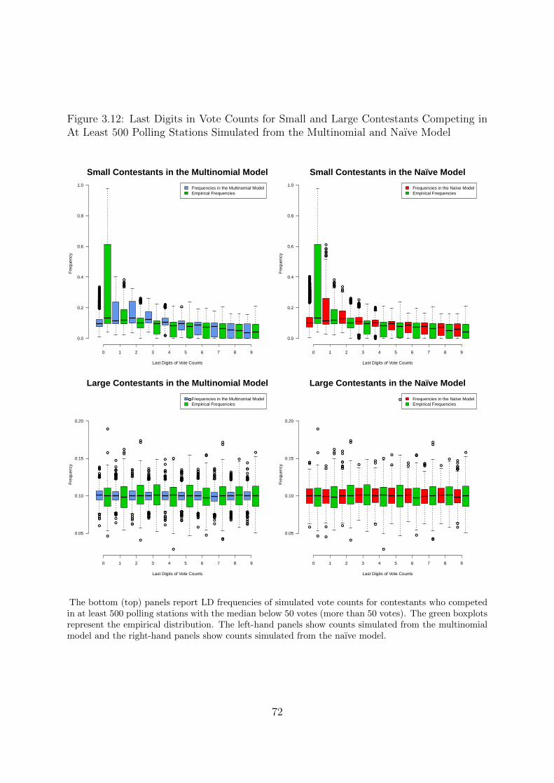
Figure 3.12: Last Digits in Vote Counts for Small and Large Contestants Competing inAt Least 500 Polling Stations Simulated from the Multinomial and Naıve Model
●
●●●
●
●
●
●●●●
●
●●●
●●
●
●●
●●
●●●
●
●
●●●
●
●
●●
●
●
●
●
●
●
●
●
●
●●
●●
●
●
●
●
●
●
●●●
●
●
●
●
●●
●●
●●●
●
●●
●●
●
●
●
●●
●
●●●
●
●
●
●
●
●●●●
●
●
●
●●
●
●●
●
●
●●
●
●
●
●
●
●●●●●
●
●●
●
●
●●●●●●
●
●
●
●
●
●●●●●●●
●●
●
●
●●●
●
●●●●●●
●●●●
●●
●
●
●
●●
●
●
●
●●
●
●
●●●
●
●
●●●●
●●●●
●
●
●●
●●●●
●
●●
●●
●
●
●
●
●
●
●
●●●●
●●●
●
●●●●●●●
●●●●●●●
●
●●●
●
●●
●
●●
●●●
●●●●●●●●●●●●●
●
●
●
●●●●●●●●●●●●●●●●●●●●●●●●●● ●
Small Contestants in the Multinomial Model
Last Digits of Vote Counts
Fre
quen
cy
Frequencies in the Multinomial ModelEmpirical Frequencies
0 1 2 3 4 5 6 7 8 9
0.0
0.2
0.4
0.6
0.8
1.0
●
●●●
●
●●●●●
●
●
●●●
●
●
●●
●●
●
●
●
●
●
●●
●
●●
●
●
●
●
●
●●
●
●●
●
●
●
●
●●
●●
●
●
●
●
●
●●
●
●
●●
●●●
●
●
●
●●
●●
●●
●
●
●
●
●
●
●●●
●●
●●●●
●
●●
●
●
●●
●●
●
●
●
●
●
●●
●●
●
●
●●
●●
●
●●
●
●
●
●
●
●
●
●
●●
●
●
●●
●
●●●●●●
●
●●
●●●●
●●
●●●●●●
●
●
●
●
●●●
●●●●●
●
●●
●●
●
●●●
●
●
●
●
●
●●●
●
●●
●
●●
●
●●
●
●
●
●●
●●
●
●
●●
●
●
●●
●
●
●
●●
●
●
●
●
●
●●
●
●
●
●●
●
●
●
●
●
●
●
●
●
●
●
●
●
●●●
●●
●●●●
●●●●●
●●●●●●
●
●
●●
●
●
●
●
●●
●
●●●
●
●
●
●●
●●
●
●
●●●
●
●
●
●●
●●
●
●
●
●
●
●
●
●
●●
●●
●●
●
●●●●
●
●
●
●
●
●●
●
●
●
●●
●
●
●
●●●
●
●
●●
●
●
●●●
●
●
●
●
●●
●
●
●●●●●
●
●●●
●●
●
●
●
●
●
●
●
●
●
●
●●
●●●
●
●●
●●
●
●
●
●
●
●●
●
●●
●
●
●
●
●
●
●●
●
●
●
●
●
●●
●
●
●●
●●
●
●
●●
●
●
●
●
●
●
●●
●
●
●●
●●
●
●
●
●
●●
●
●●
●●●
●
●●
●●●●●●●●●●●●●
●●●●●●●●●●●
●●●●●
●
●●●●●
●●
●●●
●●●
●
●
●●●
●●
●●
●●●●●
●●
●●●●
●●●●●●●●●●
●●●●●●●●●
●
●●●●●●
●●●
●●●
●●
●●●●●●
Small Contestants in the Naïve Model
Last Digits of Vote Counts
Fre
quen
cy
Frequencies in the Naïve ModelEmpirical Frequencies
0 1 2 3 4 5 6 7 8 9
0.0
0.2
0.4
0.6
0.8
1.0
●●
●
●
●
●
●
●
●
●
●
●
●
●
●●●●●
●
●
●
●
●
●
●
●
●
●
●
●
●●●
●
●
●
●
●●
●
●
●
●
●
●●
●
●
●
●
●●
●●●
●
●
●
●●
●●
●
●
●●
●
●
●
●●
●
●
●
●●●●
●
●
●
●●●
●●
●
●
●
●
●
●
●
●
●●
●
●
●
●
●
●
●
●
●
●●
●●
●
●●
●
●●
●
●●
●
●
●
●●●●
●
●
●
●
●
●●●●
●
●
●
●
●
●
●●
●
●
●
●●
●●
●
●
●
●
●
●
●
●
●
●
●
●
●
●●
●
●
●
●
●●
●
●
●
●
●●
●
●●
●
●
●
●
●
●●
●
●●●
●
●●
●●
●
●
●
●
●●
●
●
●
●●
●
●
●●
●
●
●
●●
●
●
●
●●
●
●
●
●
●
●●
●
●●●
●
●●●●●
●●
●●●●
●
●
●●
●
●
●
●●●
●●●
●●
●
●
●●
●●
●
●●●
●
●
●●
●●
●●
●
●●
●
●
●
●
●
●
●
●
●
●●●
●
●
●
●●
●●
●
●●●
●
●
●
●
●●
●
●
●
●
●●●
●
Large Contestants in the Multinomial Model
Last Digits of Vote Counts
Fre
quen
cy
Frequencies in the Multinomial ModelEmpirical Frequencies
0 1 2 3 4 5 6 7 8 9
0.05
0.10
0.15
0.20
●
●●●
●
●
●
●
●
●●
●●●
●●●
●
●
●
●
●●
●
●●
●
●
●●
●
●
●
●
●
●●
●
●●
●●●●
●
●●
●
●
●
●
●
●
●●●●●●
●
●
Large Contestants in the Naïve Model
Last Digits of Vote Counts
Fre
quen
cy
Frequencies in the Naïve ModelEmpirical Frequencies
0 1 2 3 4 5 6 7 8 9
0.05
0.10
0.15
0.20
The bottom (top) panels report LD frequencies of simulated vote counts for contestants who competedin at least 500 polling stations with the median below 50 votes (more than 50 votes). The green boxplotsrepresent the empirical distribution. The left-hand panels show counts simulated from the multinomialmodel and the right-hand panels show counts simulated from the naıve model.
72
Appendix C: R Code
########## Useful Functions ##########
# Gets the digits at a given position (amended from Beber and Scacco
[2012])
#
# Parameters:
# ’v’ - the input vector
# ’pos ’ - 1 for the FSD , 2 for the SSD , "last" for LD
# ’percentage ’ - should be set to TRUE for ’v’ being vote shares and
set to FALSE for ’v’ being vote counts
get.digits <- function(v, pos = 1, percentage = FALSE) {
if(!pos %in% c("last", "penult ") & !is.numeric(pos)) stop(" Invalid
position ")
if(pos == "last"){
s <- strsplit(as.character(v), c())
out <- sapply(s, function(y) y[length(y)])
}
if(is.numeric(pos)){
if(pos == 1){
if(percentage == TRUE){
while (sum(0<v & v<1, na.rm = TRUE) >0) v[which(0<v & v<1)] <-
10*v[which(0<v & v<1)]
}
s <- strsplit(as.character(v[v>0]), c())
out <- sapply(s, function(y) y[pos])
}
if(pos == 2){
if(percentage == TRUE){
while (sum(0<v & v<10, na.rm = TRUE) >0) v[which(0<v & v<10)] <-
10*v[which(0<v & v<10)]
}
s <- strsplit(as.character(v[v >=10]) , c())
out <- sapply(s, function(y) y[pos])
}
}
return(out)
}
73

# Formats the output from get.digits () conveniently
#
# The parameters are passed to get.digits ():
# ’v’ to ’v’
# ’po’ to ’pos ’
# ’pe’ to ’percentage ’
get.digits.table <- function(v, po = 1, pe = FALSE){
x <- table(get.digits(v, pos = po, percentage = pe))
y <- x
if (po == 1){
if (length(names(x)) != 9){
y <- c(x,rep(0,9-length(names(x))))
names(y) <- c(names(x) ,(1:9)[-as.numeric(names(x))])
y <- y[order(as.numeric(names(y)))]
}
}
if (po == 2){
if (length(names(x)) != 10){
y <- c(x,rep(0,10- length(names(x))))
names(y) <- c(names(x) ,(0:9)[-c(as.numeric(names(x))+1)])
y <- y[order(as.numeric(names(y)))]
}
}
if (po == "last"){
if (length(names(x)) != 10){
y <- c(x,rep(0,10- length(names(x))))
names(y) <- c(names(x) ,(0:9)[-c(as.numeric(names(x))+1)])
y <- y[order(as.numeric(names(y)))]
}
}
y
}
# Computes the p-value of Pearson Chi^2 Test for Digital Frequencies
#
# Parameters:
# ’x’ - a vector of digital frequencies , typically an output of get.
digits.table()
# ’distr ’ - the digital pattern to be checked
pvalue <- function(x, distr = c("1BL", "2BL", "LDU")){
if (distr == "1BL"){
a <- round (1 - pchisq( sum((c(x-(log10 (2:10) -log10 (1:9))[as.numeric
(names(x))]*sum(x), (log10 (2:10) -log10 (1:9))[-c(as.numeric(names
(x)))]*sum(x)))^2/(( log10 (2:10) -log10 (1:9))*sum(x))), 8), digits
= 3)
}
if (distr == "2BL"){
74
a <- round (1 - pchisq( sum((c(x- c
(0.12 ,0.114 ,0.108 ,0.104 ,0.1 ,0.097 ,0.093 ,0.09 ,0.088 ,0.085)[as.
numeric(names(x))+1]* sum(x), sum(x)*c
(0.12 ,0.114 ,0.108 ,0.104 ,0.1 ,0.097 ,0.093 ,0.09 ,0.088 ,0.085)[-c((as
.numeric(names(x))+1))]))^2/(c
(0.12 ,0.114 ,0.108 ,0.104 ,0.1 ,0.097 ,0.093 ,0.09 ,0.088 ,0.085)*sum(x)
)), 9), 3)
}
if (distr == "LDU"){
a <- round(1 - pchisq( sum((c(x- rep (0.1 ,10)[as.numeric(names(x))
+1]* sum(x),rep (0.1 ,10)[-(as.numeric(names(x))+1)]*sum(x) ))
^2/( rep (0.1 ,10)*sum(x))), 9), 3)
}
a
}
# Selects only polling Stations with sensible results (takes a pre -
formatted data frame on the input)
clean <- function(x){
if (" Voters" %in% colnames(x)) x <- x[x$Voters != 0,]
if (" Votes" %in% colnames(x)) x <- x[x$Votes != 0,]
if (" Valid" %in% colnames(x)) x <- x[x$Valid != 0,]
if (" Valid" %in% colnames(x)) x <- x[!is.na(x$Valid),]
x
}
# Computes sensitivities and specificities for ROC curves
#
# Parameters:
# ’pred ’ - vector of predicted class probabilities
# ’true ’ - true class labels
compute.SS <- function(pred , true){
cvec <- seq (0.000 , 1, length = 1001)
specif <- numeric(length(cvec))
sensit <- numeric(length(cvec))
for (i in 1: length(cvec)){
sensit[i] <- sum(pred > cvec[i] & true ==1)/sum(true ==1)
specif[i] <- sum(pred <=cvec[i] & true ==0)/sum(true ==0)
}
data.frame(sensit , specif)
}
# Plots cummulative ROC curves (needs package {fields }) from a
specificity and a sensitivity vector taken as inputs in this order
prepare.ROCs <- function(x, y){
a <- 0:200
b <- 0:200
75
z <- as.matrix(expand.grid(a,b))
colnames(z) <- c(" Specificity", "Sensitivity ")
m <- length(a)
zsums <- rep(0,m^2)
for (i in 1: length(x)){
x1 <- sapply(x[[i]], function(z) floor (200*z))
y1 <- sapply(y[[i]], function(z) floor (200*z))
for (j in 1: length(x[[i]])){
zsums[z[,1] == x1[j] & z[,2] == y1[j]] <- zsums[z[,1] == x1[j] &
z[,2] == y1[j]] + 1
}
}
plot.surface(list(x = Specificity = a/200, y = Sensitivity = b/200, z
= matrix(zsums ,m,m)), type = "I")
}
########## Example of Ad Hoc Data Manipulation and Cleaning of a
Preprocessed .csv File with Election Results for a Single Election (
Canada , Lower House , 2006) ##########
C2006 <- rep( list(list(list())), 308 )
files <- list.files(pattern =".csv")
j <- 1
for (f in files){
C2006[[j]] <- read.csv(f,as.is = TRUE)
j <- j + 1
}; rm(j)
C2006 <- lapply(C2006 , function(x) x[,c(1, 4, 10, 11, 14, 18)])
for (i in 1:308){
for (j in 1:dim(C2006[[i]]) [1]){
if (C2006[[i]][j,5] == "Independent ") C2006[[i]][j,5] <- paste(
C2006[[i]][j,4],C2006 [[i]][j,5],sep = ".")
}
}
C2006 <- lapply(C2006 , function(x) x[,-4])
for (i in 1:308){
colnames(C2006 [[i]]) <- c(" Level2", "Level1", "Voters", "C", "Gains ")
}
C2006x <- lapply(C2006 , reshape , direction = "wide", idvar = c(" Level2
", "Level1", "Voters "), v.names = "Gains", timevar = "C" )
76
x <- C2006x [[1]]
for (i in 2:308){
x <- merge(x, C2006x [[i]], all = TRUE)
}
x$Valid <- apply(x[,4:103],1,sum , na.rm = TRUE)
CAN2006H <- x[,c(1:3 ,104 ,4:15 ,17 ,16 ,18:103)]
for (i in 5:104){
colnames(CAN2006H)[i] <- paste ("C",i-4,sep = "")
}
save(CAN2006H , file = "CAN2006H.rData")
########## Example of Data Manipulation in the Emirical Analysis
##########
# Finds all files in the folder (relating to different elections)
files <- list.files(pattern = ".rData ")
# Loads all the elections into a single list and name it
k <- 0
psd <- rep(list(list()), length(files))
for (i in 1: length(files)){
load(files[i])
k <- k+1
psd[[k]] <- get(substr(files[i],1,nchar(files[i]) -6))
names(psd)[k] <- load(files[i])
}
# Restructures the list by column ’Const ’ into a matrix with the
digital distribution of the FSDs of all contestants in all elections
. Each distribution is represented by a single row.
FSDc <- get.digits.table(psd [[1]]$C1 , po = 1)
n <- paste(names(psd)[1], "C1", sep = " ")
s1a <- median(psd [[1]]$C1 , na.rm = TRUE)
s1b <- mean(psd [[1]]$C1 , na.rm = TRUE)
for (j in colnames(psd [[1]])[substr(colnames(psd [[1]]) ,1,1)=="C" &
colnames(psd [[1]]) != "Const" ][ -1]){
FSDc <- rbind(FSDc ,get.digits.table(psd [[1]][ ,j]))
n <- c(n, paste(names(psd)[1], j, sep = " "))
s1a <- c(s1a , median(psd [[1]][ ,j], na.rm = TRUE))
s1b <- c(s1b , mean(psd [[1]][ ,j], na.rm = TRUE))
}
for (i in 2:79){
77

if (" Const" %in% colnames(psd[[i]])){
for (j in colnames(psd[[i]])[substr(colnames(psd[[i]]) ,1,1)=="C" &
colnames(psd[[i]]) != "Const "]){
for (k in unique(psd[[i]] $Const)){
FSDc <- rbind(FSDc ,get.digits.table(psd[[i]][ psd[[i]] $Const ==
k,j]))
n <- c(n, paste(names(psd)[i],k, j, sep = " "))
s1a <- c(s1a ,median(psd[[i]][psd[[i]] $Const == k,j], na.rm =
TRUE))
s1b <- c(s1b ,mean(psd[[i]][psd[[i]] $Const == k,j], na.rm = TRUE
))
}
}
}
else{
for (j in colnames(psd[[i]])[substr(colnames(psd[[i]]) ,1,1)=="C" &
colnames(psd[[i]]) != "Const "]){
FSDc <- rbind(FSDc ,get.digits.table(psd[[i]][,j]))
n <- c(n, paste(names(psd)[i],"N", j, sep = " "))
s1a <- c(s1a ,median(psd[[i]][,j], na.rm = TRUE))
s1b <- c(s1b ,mean(psd[[i]][,j], na.rm = TRUE))
}
}
}
########## Synthetic Data Analysis ##########
library(compositions)
##### Data Preparation
# Loads the data for all fraud -free elections
files <- list.files(pattern = ".rData ")
files <- files [!( files %in% c(" AFG2009P1.rData","CHI1924P.rData","
CHI1928P.rData","NIG2003P1.rData","RUS2003H.rData","RUS2007H.rData
","RUS2011H.rData"," RUS2012P1.rData"," SIE2012P1.rData"," UGA2011P1.
rData "))]
# Loads the elections into a single list
k <- 0
psd <- rep(list(list()), length(files))
for (i in 1: length(files)){
load(files[i])
k <- k+1
psd[[k]] <- get(substr(files[i],1,nchar(files[i]) -6))
names(psd)[k] <- load(files[i])
78

}
# Creates a list of election contests rather than elections
psdc <- split(psd [[1]], psd [[1]] $Const)
names(psdc) <- paste(names(psd)[1], 1: length(unique(psd [[1]] $Const)))
for (i in 2: length(psd)){
if (" Const" %in% colnames(psd[[i]])){
x <- split(psd[[i]],psd[[i]] $Const)
names(x) <- paste(names(psd)[i], 1: length(unique(psd[[i]] $Const)))
psdc <- c(psdc , x)
}
else{
x <- psd[i]
names(x) <- names(psd)[i]
psdc <- c(psdc , x)
}
}
# Only takes vote counts
for (i in 1: length(psdc.clean)){
psdc.clean[[i]] <- psdc.clean[[i]][, colnames(psdc.clean[[i]])[substr(
colnames(psdc.clean [[i]]) ,1,1) == "C" & colnames(psdc.clean [[i]])
!= "Const" ]
]
}
# Gets rid of the columns that only contain missing values
for (i in 1: length(psdc.clean)){
psdc.clean[[i]] <- psdc.clean[[i]][,! apply(psdc.clean[[i]],2, function
(x) all(is.na(x)))]
}
# Recodes NAs to NaNs
for (i in 1: length(psdc.clean)){
for (j in 1:dim(psdc.clean[[i]]) [2]){
psdc.clean [[i]][is.na(psdc.clean[[i]][,j]),j] <- NaN
}
}
# Add 1 vote to absolutely every vote count everywhere to deal with 0s
psdcp <- psdc.clean
for (i in 1: length(psdcp)){
psdcp[[i]] <- psdcp [[i]]+1
}
# Transform into compositions
psdcpa <- rep(list(list()), length(psdcp))
for (i in 1: length(psdcp)){
psdcpa [[i]] <- acomp(psdcp[[i]], MAR = NaN)
79
}
names(psdcpa) <- names(psdcp)
# Computes valid votes from +1 counts
vvcpa <- rep(list(list()), length(psdcp))
for (i in 1: length(psdcp)){
vvcpa[[i]] <- apply(psdcp [[i]], 1, sum , na.rm = TRUE)
}
names(vvcpa) <- names(psdcp)
##### NDS Goodness of Fit Assessments
# Creates QQ-plots for the fit of NDS all election contests
inapplicable <- NA
for (i in 1: length(psdcpa)){
if ( sum(missingSummary(psdcpa [[i]])[,3]) == 0 ){
pdf(paste(names(psdcpa)[i],"pdf", sep = "."))
qqnorm(psdcpa [[i]])
dev.off()
}
else inapplicable <- c(inapplicable , names(psdcpa)[i])
}
# p-values for the NDS tests of fit
px <- rep(NA ,length(psdcpa))
for (i in 1: length(psdcpa)){
if( dim(psdcpa [[i]]) [2] > 2 ) px[i] <- acompNormalGOF.test(psdcpa [[i
]])$p.value
}
##### Fraudulent Data Simulation
# Fits a compositional regression model to each election contest and
simulates 1,500 new election contests from it. It only retains the
digital information and some descriptive statistics.
for (i in 1: length(psdcpa)){
# Prepare useful objects
vvi <- vvcpa[[i]]
l <- length(vvi)
nc <- dim(psdcpa [[i]]) [2]
allffcontests <- matrix(NA ,1500 ,52*nc)
# Fits a model
model <- lm(ilr(psdcpa [[i]])~log(vvi))
80
# Computes the parameters for data simulation
if (nc==2) smeans <- ilrInv(matrix(predict(model)),orig=psdcpa [[i]])
else smeans <- ilrInv(predict(model),orig=psdcpa [[i]])
if (nc==2) varEpsilon = ilrvar2clr(matrix(var(model))) else
varEpsilon = ilrvar2clr(var(model))
for (j in 1:1500){
# Simulates a new election contest
ffcontestp <- rmult(rnorm.acomp(l,smeans ,varEpsilon))
ffcontest <- rmult(ceiling(vvi*ffcontestp) -1)
ffcontestp <- 10000* ffcontest/vvi
# Adds some descriptive statistics about the contestants
allffcontests[j,1:nc] <- apply(ffcontest , 2, median) # median votes
allffcontests[j,(nc+1) :(2*nc)] <- apply(ffcontest , 2, function(x)
median(x/vvi) ) # median percentage
# 1BL vote counts
allffcontests[j,(2*nc+1) :(11* nc)] <- round(
as.vector(apply(ffcontest , 2,
function(x){
y <- get.digits.table(x, po = 1, pe = FALSE)
y/sum(y)
})) ,5)
# 2BL vote counts
allffcontests[j,(11* nc+1) :(21* nc)] <- round(
as.vector(apply(ffcontest , 2,
function(x){
if (all(x<10)) z <- rep(NA ,10)
else{
y <- get.digits.table(x, po = 2, pe = FALSE)
z <- y/sum(y)
}
z
})) ,5)
# LDU vote counts
allffcontests[j,(21* nc+1) :(31* nc)] <- round(
as.vector(apply(ffcontest , 2,
function(x){
y <- get.digits.table(x, po = "last", pe =
FALSE)
y/sum(y)
})) ,5)
# 1BL vote shares
allffcontests[j,(31* nc+1) :(40* nc)] <- round(
as.vector(apply(ffcontestp , 2,
function(x){
y <- get.digits.table(x, po = 1, pe = TRUE)
y/sum(y)
})) ,5)
81
# 2BL vote shares
allffcontests[j,(40* nc+1) :(50* nc)] <- round(
as.vector(apply(ffcontestp , 2,
function(x){
y <- get.digits.table(x, po = 2, pe = TRUE)
y/sum(y)
})) ,5)
# More descriptive statistics
allffcontests[j,(50* nc+1) :(51* nc)] <- apply(ffcontest , 2, sum , na.
rm = TRUE)
allffcontests[j,(51* nc+1) :(52* nc)] <- apply(ffcontest , 2, function(
x) sum(na.omit(x) >10))
}
# Saves theobject with the correct name
save(allffcontests , file = paste(names(psdcpa)[i]," FF", sep ="" ,".
rData ") )
}
##### Fraud -Imputed Data Simulation
# Sets the parameter values
delta <- 1.5
gamma <- 0.1
for (i in 1: length(psdcpa)){
# Prepare useful objects
vvi <- vvcpa[[i]]
l <- length(vvi)
nc <- dim(psdcpa [[i]]) [2]
allffcontests <- matrix(NA ,1500 ,53*nc)
# Ranks the contestants by size
sizes <- order(apply(psdcpa [[i]],2,sum ,na.rm = TRUE),decreasing =
TRUE)
# Fits a model
model <- lm(ilr(psdcpa [[i]])~log(vvi))
# Computes the predicted compositions for all valid votes
if (nc==2) smeans <- ilrInv(matrix(predict(model)),orig=psdcpa [[i]])
else smeans <- ilrInv(predict(model),orig=psdcpa [[i]])
if (nc==2) varEpsilon = ilrvar2clr(matrix(var(model))) else
varEpsilon = ilrvar2clr(var(model)) # for both variances
82
for (j in 1:1500){
# Simulate a new election contest
ffcontestp <- rmult(rnorm.acomp(l,smeans ,varEpsilon))
ffcontest <- rmult(ceiling(vvi*ffcontestp) -1)
if (nc == 2) opposition <- apply(matrix(ffcontest[,-sizes [1]]) ,1,
sum , na.rm = TRUE)
else opposition <- apply(ffcontest[,-sizes [1]],1,sum , na.rm = TRUE)
# Move to a new object
frcontest <- ffcontest
# Get the fraudulent votes of the strongest contestant
frcontest[,sizes [1]] <- round(ffcontest[,sizes [1]] + delta*gamma*
opposition)
# Sample the votes to take from the smaller contestants
if (nc == 2){
votes <- lapply(apply(matrix(ffcontest[,-sizes [1]]) ,1, function(x
) rep (1:(nc -1), times = x)),
function(x) sample(x, size = round(gamma*length(x
)))
)
}
else {
votes <- lapply(apply(ffcontest[,-sizes [1]],1, function(x) rep
(1:(nc -1), times = x)),
function(x) sample(x, size = round(gamma*length(x
)))
)
}
# Get the numbers per contestant
transfers <- lapply(votes ,table)
# Convenient formatting
alltransfers <- matrix(
sapply(transfers , function(xxx){
if (length(names(xxx)) != nc -1){
y <- c(xxx ,rep(0,nc -1-length(names(xxx))))
names(y) <- c(names(xxx) ,(1:(nc -1))[-as.numeric(names(xxx))])
y <- y[order(as.numeric(names(y)))]
}
else xxx
}
),length(transfers) , nc -1, byrow = TRUE)
# Transfer votes away from smaller contestants and get the final
vote counts
frcontest[,-sizes [1]] <- ffcontest[,-sizes [1]] - alltransfers
ffcontest <- frcontest
# Get the vote shares
83
ffcontestp <- 10000* frcontest/apply(frcontest ,1,sum , na.rm = TRUE)
# Adds some descriptive statistics about the contestants
allffcontests[j,1:nc] <- apply(ffcontest , 2, median)
allffcontests[j,(nc+1) :(2*nc)] <- apply(ffcontest , 2, function(x)
median(x/vvi) )
# 1BL vote counts
allffcontests[j,(2*nc+1) :(11* nc)] <- round(
as.vector(apply(ffcontest , 2,
function(x){
y <- get.digits.table(x, po = 1, pe = FALSE)
y/sum(y)
})) ,5)
# 2BL vote counts
allffcontests[j,(11* nc+1) :(21* nc)] <- round(
as.vector(apply(ffcontest , 2,
function(x){
if (all(x<10)) z <- rep(NA ,10)
else{
y <- get.digits.table(x, po = 2, pe = FALSE)
z <- y/sum(y)
}
z
})) ,5)
# LDU vote counts
allffcontests[j,(21* nc+1) :(31* nc)] <- round(
as.vector(apply(ffcontest , 2,
function(x){
y <- get.digits.table(x, po = "last", pe =
FALSE)
y/sum(y)
})) ,5)
# 1BL vote shares
allffcontests[j,(31* nc+1) :(40* nc)] <- round(
as.vector(apply(ffcontestp , 2,
function(x){
y <- get.digits.table(x, po = 1, pe = TRUE)
y/sum(y)
})) ,5)
# 2BL vote shares
allffcontests[j,(40* nc+1) :(50* nc)] <- round(
as.vector(apply(ffcontestp , 2,
function(x){
y <- get.digits.table(x, po = 2, pe = TRUE)
y/sum(y)
})) ,5)
# More descriptive statistics
allffcontests[j,(50* nc+1) :(51* nc)] <- apply(ffcontest , 2, sum , na.
rm = TRUE)
84
allffcontests[j,(51* nc+1) :(52* nc)] <- apply(ffcontest , 2, function(
x) sum(na.omit(x) >10))
allffcontests[j,(52* nc+1) :(53* nc)] <- sizes
}
# Saves the Object
save(allffcontests , file = paste(names(psdcpa)[i]," FR33", sep ="" ,".
rData ") )
}
########## Regressions and Results ##########
##### Regression Analysis (an example of multinomial regressions for
fruad types)
library(nnet)
# Prepare useful objects
MultinomResults <- rep(list(list()), length(filesTEST))
drops.in.deviance <- rep(list(list()), length(filesTEST))
npars <- rep(list(list()), length(filesTEST))
# Runs the regressions
for (i in 1: length(filesTEST)){
load( filesTEST[i] )
load( filesTRAIN[i])
# Gets the appropriate data
trainingData <- trainingData[c(1:1000 ,3001:4000 ,5001:8000) ,]
testData <- testData[c(1:500 ,1501:2000 ,2501:4000) ,]
f1 <- factor(trainingData$fraud , levels = 0:5)
trainingData <- trainingData[,substr(colnames(trainingData) ,1,1) == "
M"]
trainingData[, apply(trainingData ,2,sd) != 0] <- scale(trainingData[,
apply(trainingData ,2,sd) != 0])
trainingData$fraud <- f1
f2 <- factor(testData$fraud , levels = 0:5)
testData <- testData[,substr(colnames(testData) ,1,1) == "M"]
testData[, apply(testData ,2,sd) != 0] <- scale(testData[, apply(
testData ,2,sd) != 0])
testData$fraud <- f2
85

# Fits the full model
model0 <- multinom(fraud ~ . , data = trainingData , MaxNWts = 10000,
maxit = 10000)
class0 <- predict(model0 , testData , type = "class")
deviance0 <- deviance(model0)
# Fits the submodels
model1 <- multinom(fraud ~ . , data = trainingData[, substr(colnames(
trainingData) ,2,3) != "1v"], MaxNWts = 10000, maxit = 10000)
deviance1 <- deviance(model1)
model2 <- multinom(fraud ~ . , data = trainingData[, substr(colnames(
trainingData) ,2,3) != "2v"], MaxNWts = 10000, maxit = 10000)
deviance2 <- deviance(model2)
model3 <- multinom(fraud ~ . , data = trainingData[, substr(colnames(
trainingData) ,2,3) != "lv"], MaxNWts = 10000, maxit = 10000)
deviance3 <- deviance(model3)
model4 <- multinom(fraud ~ . , data = trainingData[, substr(colnames(
trainingData) ,2,3) != "1s"], MaxNWts = 10000, maxit = 10000)
deviance4 <- deviance(model4)
model5 <- multinom(fraud ~ . , data = trainingData[, substr(colnames(
trainingData) ,2,3) != "2s"], MaxNWts = 10000, maxit = 10000)
deviance5 <- deviance(model5)
# Gets the numbers of predictors for each digital pattern
npars1 <- table(substr(colnames(trainingData) ,2,3))["1v"]
npars2 <- table(substr(colnames(trainingData) ,2,3))["2v"]
npars3 <- table(substr(colnames(trainingData) ,2,3))["lv"]
npars4 <- table(substr(colnames(trainingData) ,2,3))["1s"]
npars5 <- table(substr(colnames(trainingData) ,2,3))["2s"]
# Gets the Output
drops.in.deviance [[i]] <- c(deviance1 , deviance2 , deviance3 ,
deviance4 , deviance5) - deviance0
npars[[i]] <- c(npars1 , npars2 , npars3 , npars4 , npars5)
MultinomResults [[i]] <- table(predicted = class0 , true =
testData$fraud)
}
##### Deviance Analysis
# Gets the differences in deviances and the numbers of predictors for
digital patterns
86
files <- list.files(pattern = ".rData ")
load(files [6])
np <- npars [1:400]
DD <- drops.in.deviance [1:400]
k <- 1
for (i in files[c(7:14 ,1:5)]){
load(i)
np <- c(np , npars[
list
(401:800 ,801:1200 ,1201:1600 ,1601:2000 ,2001:2400 ,2401:2800 ,2801:3200 ,
3201:3600 ,3601:4000 ,4001:4400 ,4401:4800 ,4801:5200 ,5201:5620) [[
k]]
])
DD <- c(DD , drops.in.deviance[
list
(401:800 ,801:1200 ,1201:1600 ,1601:2000 ,2001:2400 ,2401:2800 ,2801:3200 ,
3201:3600 ,3601:4000 ,4001:4400 ,4401:4800 ,4801:5200 ,5201:5620) [[
k]]
])
k <- k + 1
}
# Prepares the data for plotting
Dpv <- matrix(0,length(np) ,5)
Ddev <- matrix(0,length(np) ,5)
for (i in 1: length(np)){
Dpv[i,] <- (1-pchisq(DD[[i]], np[[i]]))[c(4:5 ,1:3)]
Ddev[i,] <- (DD[[i]])[c(4:5 ,1:3)]
}
# Plots the values
pdf(" deviance.pdf", width = 14, height = 7)
par(mfrow = c(1,2))
plot(apply(Dpv ,2,function(x) 100* sum(x <0.01)/length(x)), type = "b",
ylim = c(0 ,100), xlab = "Digital Pattern",
ylab = "Percentage of p-Values Below 0.01", col = "cornflowerblue
", main = "Difference in Deviances Tests ",
axes = FALSE , cex.main = 1.3, cex.lab = 1.3)
axis(2, las = 2)
axis(1,at = 1:5, labels = c(" Shares FSD", "Shares SSD", "Counts FSD", "
Counts SSD", "Counts LD"))
boxplot(apply(Ddev ,2,function(x) log10(x+1)), axes = FALSE , xlab = "
Digital Pattern",
ylab = "Difference In Deviances", main = "Difference In
Deviances",
cex.main = 1.3, cex.lab = 1.3, las = 1, col = "darkolivegreen3
")
87
axis(2, at = c(0,log10(c(11 ,101 ,1001 ,10001)), labels = c(0 ,10^(1:4)),
las = 2)
axis(1,at = 1:5, labels = c(" Shares FSD", "Shares SSD", "Counts FSD", "
Counts SSD", "Counts LD"))
dev.off()
##### Preparation and Construction of the Violin Plots
# Gets and formats the data
load(files [6])
MR <- MultinomResults [1:400]
k <- 1
for (i in files[c(7:14 ,1:5)]){ #files[c(7:14 ,2:5)]
load(i)
MR <- c(MR , MultinomResults[
list
(401:800 ,801:1200 ,1201:1600 ,1601:2000 ,2001:2400 ,2401:2800 ,2801:3200 ,
3201:3600 ,3601:4000 ,4001:4400 ,4401:4800 ,4801:5200 ,5201:5620) [[
k]]
])
k <- k + 1
}
# Prepares and constructs a the plots
MR1 <- lapply(MR ,t)
ToM <- matrix (0,6,6)
ToSD <- matrix (0,6,6)
LoF <- rep(list(list()), 36 )
pdf(" finalplottogl.pdf",width = 12, height = 16)
a <- rep(list(list()) ,6)
par(mfrow = c(6,1))
for (i in 1:6){
for (j in 1:6){
ToM[i,j] <- mean(sapply(MR1 , function(x) x[i,j]/5))
ToSD[i,j] <- sd(sapply(MR1 , function(x) x[i,j]/5))
a[[j]] <- sapply(MR1 , function(x) x[i,j]/5)
}
col.vector <- rep(" cornflowerblue ",6)
col.vector[i] <- "darkolivegreen3"
names.vector <- c(expression(paste(gamma , " = 0, ", delta , " = 0")),
expression(paste(gamma , " = 0.01, ", delta , " = 1.01")),
expression(paste(gamma , " = 0.05, ", delta , " =
1.05")),expression(paste(gamma , " = 0.1, ",
delta , " = 1.1")),
expression(paste(gamma , " = 0.3, ", delta , " =
1.3")),expression(paste(gamma , " = 0.5, ", delta
, " = 1.5")))
88
expressions.vector <- list(expression(paste (" Classifications of True
(", gamma , " = 0, ", delta , " = 0)", " Classes (in %)"), sep = "")
,
expression(paste (" Classifications of True
(", gamma , " = 0.01, ", delta , " =
1.01)", " Classes (in %)"), sep = ""),
expression(paste (" Classifications of True
(", gamma , " = 0.05, ", delta , " =
1.05)", " Classes (in %)"), sep = ""),
expression(paste (" Classifications of True
(", gamma , " = 0.1, ", delta , " = 1.1)
", " Classes (in %)"), sep = ""),
expression(paste (" Classifications of True
(", gamma , " = 0.3, ", delta , " = 1.3)
", " Classes (in %)"), sep = ""),
expression(paste (" Classifications of True
(", gamma , " = 0.5, ", delta , " = 1.5)
", " Classes (in %)"), sep = ""))
myvioplot(a[[1]] , a[[2]] , a[[3]] , a[[4]] , a[[5]] , a[[6]] , drawRect=
FALSE ,
col = col.vector , ylim = c(0 ,100), names = names.vector)
title(expressions.vector [[i]], cex.main = 2)
}
dev.off()
89