NREL is a national laboratory of the U.S. Department of Energy Office of Energy Efficiency & Renewable Energy Operated by the Alliance for Sustainable Energy, LLC This report is available at no cost from the National Renewable Energy Laboratory (NREL) at www.nrel.gov/publications.

Contract No. DE-AC36-08GO28308

Technical Report NREL/TP-6A20-71912 January 2019

The Potential Role of Concentrating Solar Power within the Context of DOE’s 2030 Solar Cost Targets

Caitlin Murphy, Yinong Sun, Wesley Cole, Galen Maclaurin, Craig Turchi, and Mark Mehos

National Renewable Energy Laboratory

NREL is a national laboratory of the U.S. Department of Energy Office of Energy Efficiency & Renewable Energy Operated by the Alliance for Sustainable Energy, LLC This report is available at no cost from the National Renewable Energy Laboratory (NREL) at www.nrel.gov/publications.

Contract No. DE-AC36-08GO28308

National Renewable Energy Laboratory 15013 Denver West Parkway Golden, CO 80401 303-275-3000 • www.nrel.gov

Technical Report NREL/TP-6A20-71912 January 2019

The Potential Role of Concentrating Solar Power within the Context of DOE’s 2030 Solar Cost Targets

Caitlin Murphy, Yinong Sun, Wesley Cole, Galen Maclaurin, Craig Turchi, and Mark Mehos

National Renewable Energy Laboratory

Suggested Citation Murphy, Caitlin, Yinong Sun, Wesley Cole, Galen Maclaurin, Craig Turchi, and Mark Mehos. 2019. The Potential Role of Concentrating Solar Power within the Context of DOE’s 2030 Solar Cost Target. Golden, CO: National Renewable Energy Laboratory. NREL/TP-6A20-71912. https://www.nrel.gov/docs/fy19osti/71912.pdf.

NOTICE

This work was authored by the National Renewable Energy Laboratory, operated by Alliance for Sustainable Energy, LLC, for the U.S. Department of Energy (DOE) under Contract No. DE-AC36-08GO28308. Funding provided by the U.S. Department of Energy Office of Energy Efficiency and Renewable Energy Solar Energy Technologies Office. The views expressed herein do not necessarily represent the views of the DOE or the U.S. Government.

This report is available at no cost from the National Renewable Energy Laboratory (NREL) at www.nrel.gov/publications.

U.S. Department of Energy (DOE) reports produced after 1991 and a growing number of pre-1991 documents are available free via www.OSTI.gov.

Cover Photos by Dennis Schroeder: (clockwise, left to right) NREL 51934, NREL 45897, NREL 42160, NREL 45891, NREL 48097, NREL 46526.

NREL prints on paper that contains recycled content.

iii This report is available at no cost from the National Renewable Energy Laboratory (NREL) at www.nrel.gov/publications.

Acknowledgments We gratefully acknowledge the many people whose efforts contributed to this report. Many NREL colleagues reviewed and improved this report, including Doug Arent, Gian Porro, Daniel Steinberg, Jennie Jorgenson, Ben Sigrin, and Parthiv Kurup. We are also grateful to our external reviewers for providing feedback on this work through an external peer review process, including Sam Baldwin, Becca Jones-Albertus, Guohui Yuan, and Paul Spitsen from DOE, and Chris Namovic (U.S. Energy Information Administration), Brad Albert (Arizona Public Service Company), Charles Rossman and Will Hobbs (Southern Company), Aaron Townsend (Electric Reliability Council of Texas), Andrew Arana (Florida Power and Light), David Young (Electric Power Research Institute), Adam Green (SolarReserve), and Justin Baca and Rachel Goldstein (Solar Energy Industries Association). We especially thank Abraham (Avi) Shultz (DOE) for his leadership and insights relating to the work presented in this report.

iv This report is available at no cost from the National Renewable Energy Laboratory (NREL) at www.nrel.gov/publications.

Executive Summary The U.S. Department of Energy (DOE) has research programs to improve the cost and performance of a diverse portfolio of electricity generating technologies. Success in each of DOE’s research programs could result in aggressive reductions in the costs and emissions associated with the U.S. power sector. The analysis reported here is designed to evaluate and isolate the potential impacts of success within DOE’s research program for solar electricity generating technologies; it does not reflect the potential benefits or system impacts associated with success in other DOE research programs.

For solar electricity generating technologies to be cost competitive at a large scale with conventionally generated electricity, cost reductions are needed for both concentrating solar power (CSP) and solar photovoltaic (PV) systems. PV technology converts sunlight directly into electricity, whereas CSP uses mirrors or lenses to generate high-temperature thermal energy from concentrated sunlight. This energy can be used, in turn, to drive turbines, producing electricity in a manner similar to that used in conventional thermal power plants. When coupled with energy storage systems, both PV and CSP plants can generate electricity on demand. In particular, PV can be coupled with any electricity storage technology, while CSP is typically paired with thermal energy storage (CSP-TES); both approaches allow solar plants to dispatch electricity after sunset, before sunrise, and during extended cloudy periods.

Early solar deployments were driven by policies such as the Public Utility Regulatory Policies Act, state-based renewable portfolio standards, a 30% federal investment tax credit, and federal loan guarantees. More recently, reductions in module prices have made modest levels of PV cost-competitive in many parts of the contiguous United States, particularly where it is competing with higher-priced conventional generators and there is moderate to good solar resource (DOE 2017). To date, PV deployments total approximately 44 GW,1 and they exist in all 50 states (EIA 2018b). In addition, roughly 2 GW of CSP capacity are in place in the United States, mostly in the high-solar resource Southwest (Figure ES-1).

In 2011, DOE established solar cost targets that corresponded to reducing CSP and PV prices by approximately 75% in order to achieve a levelized cost of electricity (LCOE) of $0.06 per kilowatt-hour (kWh) for both utility-scale PV and high-capacity factor CSP-TES systems in 2020.2 To examine the implications of achieving this goal, DOE’s Solar Energy Technologies Office published the SunShot Vision Study (DOE 2012), which found that achieving the 2020 cost targets could result in significant solar penetration by 2030.

Utility-scale PV achieved its 2020 cost target in 2017 (DOE 2017), and its deployment to date has exceeded levels in the SunShot Vision Study (DOE 2012) for 2020. Recent estimates for the LCOE of CSP-TES with a molten-salt power tower system are approximately $0.10/kWh

1 All capacities in this report are in terms of AC, not DC. 2 The LCOEs reported in this analysis did not include the federal investment tax credit (ITC), and LCOE goals were identified before the ITC was applied. The corresponding installed system costs for the 2020 cost targets (in 2010$) were $3.60/WAC for CSP with 14 hours of thermal storage and a solar multiple of 2.7, $1/WDC for utility-scale PV, $1.25/WDC for commercial rooftop PV, and $1.50/WDC for residential PV. (The solar multiple represents the extent to which extra energy can be stored and dispatched during periods with higher energy prices.)

v This report is available at no cost from the National Renewable Energy Laboratory (NREL) at www.nrel.gov/publications.

(Mehos et al. 2016) for projects that are expected to come online in 2020, which represents a substantial reduction since 2010—when the LCOE for CSP-TES was around $0.21/kWh (Mehos et al. 2016). Moreover, power purchase agreements (PPAs) in late 2017 for two international power tower systems that were designed to primarily provide peaking services approached the cost target of $0.06/kWh for 2020 (Feldman and Margolis 2018).3 However, given recent cost trajectories for other generating technologies and fuels, cost reductions for new CSP-TES would be needed for it to effectively compete with new low-cost PV, wind, and natural gas generators.

Figure ES-1. Available solar resource for the contiguous United States, based on the National

Solar Radiation Database and the Physical Solar Model, which was developed by the National Renewable Energy Laboratory (NREL)

Data in the map are from Sengupta et al. (2018).

In this study, new PV installations are considered throughout the contiguous United States, while new CSP-TES is only considered for direct normal irradiance of 5.0 kilowatt-hours per square meter per day (kWh/m2/day) and above (i.e., in all but the palest yellow band). Existing CSP plants that are larger than five megawatts (MW) are shown by

black circles, the size of which scales with plant capacity.

3 Developers of the Dubai Electricity and Water Authority (DEWA) IV CSP-TES project in Dubai were announced as the winning bidder for a 700-MW combined power tower and trough station at a PPA price of USD 0.073 per kWh. In addition, the developer of the Aurora CSP-TES project in Southern Australia signed a PPA with a price of USD 0.061 per kWh (Feldman and Margolis 2018).

vi This report is available at no cost from the National Renewable Energy Laboratory (NREL) at www.nrel.gov/publications.

Figure ES-2. Historical costs, current costs, and 2020 and 2030 cost targets for CSP-TES (top)

and PV (bottom) (DOE 2016)

vii This report is available at no cost from the National Renewable Energy Laboratory (NREL) at www.nrel.gov/publications.

To continue the momentum for cost reductions in solar technologies, DOE recently established cost targets for 2030 (Figure ES-2) that would make solar one of the lowest-cost sources of new electricity in the United States (DOE 2016). For CSP-based systems, the new targets correspond to an LCOE in 2030 of $0.05/kWh for a dispatchable, high-capacity factor CSP-TES plant configuration (“baseload” in Figure ES-2) (DOE 2016).4 This aggressive target would have been unimaginable a decade ago.5 However, building on the previously described reduction in CSP-TES costs over the past decade, recent announcements suggest the next phase of projects will continue this downward trend through lower installation costs, attractive financing, longer-duration PPAs, and the ability to capitalize on the value that the flexibility of storage brings CSP (Lilliestam and Pitz-Paal 2018). These trends have also been aided by the global nature of the CSP market, which has experienced learning from the first molten-salt power towers and increases in scale and supply chains. Nonetheless, continuing the momentum toward the 2030 cost targets will require innovations in system design associated with the solar field cost and enhancements to power block efficiency. These advances are the subject of research in the United States and around the world in heliostat design, heat-transfer and thermal storage media, and power cycle efficiency (Islam et al. 2018).

A similar target was also developed for a CSP-based configuration that more closely resembles a highly flexible “peaker plant” (Figure ES-2), which would be designed to provide more peaking services. In general, a peaker plant would have a lower capacity factor, and its configuration would likely involve a lower solar multiple—defined as the ratio between of the capacities of the solar field and the turbine—and it could involve fewer hours of storage, depending on the requirements of the system. It is important to note that such a plant is not included in this analysis because of challenges associated with representing such a configuration in the model used.6 Given interest from utilities and the CSP-TES community in a peaker plant configuration, it is anticipated that future model development and analysis will allow for the representation and assessment of a wider variety of CSP-TES configurations.

For PV systems (Figure ES-2), the corresponding 2030 cost targets are $0.03/kWh for utility-scale PV, $0.04/kWh for commercial PV, and $0.05/kWh for residential PV systems (DOE 2016). The potential impacts of achieving the 2030 PV cost targets were recently explored by Cole, Frew et al. (2017), who found significant potential for solar PV deployment and generation, especially when coupled with low-cost battery storage. In particular, they found that achieving the 2030 cost targets could result in 410 GW of PV capacity by 2030, which could rise to 970 GW by 2050. With the addition of low-cost battery storage,7 deployed PV capacity

4 The specific plant CSP-TES plant configuration for which the 2030 cost target was developed includes 14 hours of thermal energy storage and a solar multiple of 2.7. 5 See “Goals of the Solar Energy Technologies Office,” DOE, https://www.energy.gov/eere/solar/goals-solar-energy-technologies-office. 6 The ReEDS modeling in this analysis only represents CSP-TES plants with capacity factors greater than 40%, based on lower bounds for TES of six hours and solar multiples of 1.4–1.8, where the range reflects different solar resource classes. As a result of these model constraints, this analysis does not fully evaluate the cost-effectiveness of peaker-type CSP-TES configurations (which could involve much lower solar multiples and/or storage durations). 7 The representation of low-cost energy storage in this analysis is based on the low battery cost trajectory from Cole, Marcy et al. (2016), which assumes 8-hour utility scale battery storage capital costs decline to approximately $130/kWh by 2030 and approximately $100/kWh by 2050, assuming a 15-year lifetime and 85% round-trip efficiency with approximately one cycle per day.

viii This report is available at no cost from the National Renewable Energy Laboratory (NREL) at www.nrel.gov/publications.

increased to 1,600 GW of PV capacity by 2050, which provided 55% of generation in the contiguous United States in 2050.

Building on Cole, Frew et al. (2017), the analysis reported here employs scenario analysis to evaluate the potential impacts of simultaneously achieving the 2030 cost targets for PV and CSP-TES (Figure ES-3), and it includes a detailed evaluation of the role that CSP-TES could play in realizing those impacts. It is important to note that scenarios in this analysis should not be interpreted as forecasts or predictions. As previously mentioned, the aggressive 2030 solar cost targets will require innovation in technologies, systems, and financing. More generally, modeling the future electricity generation mix is inherently challenging because of simplifications that are needed to evaluate the evolution of a large, complex system. In addition, uncertainties related to future fuel prices, technology costs for other generator types, electricity demand, and policy changes (among other factors) introduce corresponding uncertainties for all capacity expansion model results.

Within the context of these challenges, the scenarios in this analysis are designed to isolate and assess the potential impacts of achieving DOE’s 2030 cost targets for CSP-TES and PV, which are represented via a roughly 50% reduction in LCOE by 2030 (from current levels) with additional cost reductions thereafter representing technology learning and/or improvements that could result from innovation (Figure ES-3).8 Isolating the impacts of achieving these targets is done by comparing many low-cost solar scenarios with a baseline scenario (ATB Mid),9 the latter of which evaluates the impacts of business-as-usual technology and fuel price trajectories over time. The LowCost-CSP-PV scenario evaluates the impacts of achieving the 2030 cost targets for CSP-TES and utility-scale, commercial, and residential PV systems. A scenario where only the CSP-TES target is met (LowCost-CSP) is also employed to (1) evaluate the specific impacts of achieving DOE’s 2030 CSP-TES cost target and (2) facilitate an assessment of the individual impacts of cost reductions in each solar technology via a comparison of the baseline (ATB Mid), LowCost-CSP, and LowCost-CSP-PV scenarios. Finally, a scenario in which CSP-TES, PV, and battery storage systems follow a low-cost trajectory (Figure ES-3; LowCost-CSP-PV-Storage) evaluates the competition and synergies between each low-cost solar technology coupled with energy storage (Table ES-1).

8 For PV, a 33% reduction between 2030 and 2050 was chosen for consistency with Cole, Frew et al. (2017). For CSP-TES, a 20% reduction between 2030 and 2050 was chosen for consistency with the technology learning rates for mature technologies in EIA (2018c). 9 The baseline scenario assumes mid-case costs for all generating technologies from NREL’s 2017 Annual Technology Baseline (ATB) with demand and fuel price assumptions taken from the 2018 Annual Energy Outlook. The solar resource is based on the most recent version of the National Solar Radiation Database (NSRDB) using the Physical Solar Model (PSM v.3.0.1), which indicates a wider geographic extent for a direct normal irradiance (DNI) of 5 kWh/m2/day—the lower threshold for this analysis—than previous NSRDB versions.

ix This report is available at no cost from the National Renewable Energy Laboratory (NREL) at www.nrel.gov/publications.

Figure ES-3. Capital cost trajectories for CSP-TES (top), utility-scale PV (bottom left), and battery storage (bottom right) technologies that define the primary low-cost solar scenarios presented

in Table ES-1 The cost trajectories for distributed PV are included in Appendix A. They include similar post-2030 cost reductions after the established cost targets are achieved. Note that the slight difference between the CSP-TES ATB Mid and Low Cost trajectories in the early years is the result of different assumed configurations for the technology in these

two trajectories.

A wide range of sensitivity scenarios are also examined to explore the impacts on solar deployment of alternate natural gas prices, retirement schedules, demand growth, renewable energy cost reductions (for wind, hydropower, and geothermal systems) and post-2030 cost reductions for CSP-TES. It is important to note that all scenarios include only current regulations and policies (e.g., state-level renewable portfolio standards, the federal investment and production tax credits,10 state- and regional-level cap-and-trade programs, net metering, and import tariffs), and they do not include the Clean Power Plan or any regulatory or policy changes in the electric power sector.

10 This includes the permanent 10% ITC for solar technologies.

x This report is available at no cost from the National Renewable Energy Laboratory (NREL) at www.nrel.gov/publications.

With these assumptions, the evolution of the contiguous U.S. electricity system is evaluated with NREL’s Renewable Energy Deployment System (ReEDS) model, which was specifically designed to represent the temporal and locational value of renewable generation technologies in the U.S. power system. ReEDS relies on system-wide least-cost optimization to estimate the type and location of future generation and transmission capacity. In addition, it accounts for the locational and temporal variations in variable renewable technologies, including the need for new transmission, curtailment, dynamic capacity value, and the need to hold operating reserves to account for the uncertainty and variability of these technologies (Eurek et al. 2016).

Figure ES-4 shows the growth in CSP-TES and PV capacity for the four primary scenarios (Table ES-1) used in this analysis. New PV capacity in the near term provides a sizeable amount of capacity value under scenarios with both the ATB Mid and low-cost solar trajectories, primarily due to its low cost and relatively flat demand-growth before 2030. Beyond the mid-2020s, PV capacity is similar across scenarios that assume the ATB Mid cost trajectory, regardless of the assumed cost trajectory for CSP-TES; similar levels of PV deployment in the baseline (ATB Mid) and LowCost-CSP scenarios reflect the large magnitude and geographic extent of available resource for cost-effective PV—some of which lies in areas that are not considered for CSP-TES in this analysis (i.e., the pale yellow shading in Figure ES-1)—even under the ATB Mid cost trajectory. In the LowCost-CSP-PV and LowCost-CSP-PV-Storage scenarios, cost reductions toward the 2030 PV cost target and beyond (Figure ES-3) result in an acceleration of new PV installations (relative to the baseline and LowCost-CSP scenarios), which occur throughout the United States (Figure ES-5).

Table ES-1. Definitions for the Primary Set of Scenarios Used in this Analysis, based on Cost Trajectories Shown in Figure ES-3

Scenario Name Scenario Definition

ATB Mid This is the baseline scenario in which ATB 2017 mid-case cost trajectories are used for all technologies, including CSP-TES and PV.

LowCost-CSP CSP-TES follows the Low Cost CSP-TES cost trajectory, while PV and batteries follow their respective mid-cost trajectories.

LowCost-CSP-PV CSP-TES and PV follow their respective low-cost trajectories, while batteries follow the mid-cost trajectory.

LowCost-CSP-PV-Storage CSP-TES, PV, and batteries follow their respective low-cost trajectories.

xi This report is available at no cost from the National Renewable Energy Laboratory (NREL) at www.nrel.gov/publications.

Figure ES-4. Cumulative capacity of CSP-TES (solid lines) and PV (dotted lines) for the baseline

(ATB Mid) and primary low-cost solar scenarios

In all scenarios that assume the trajectory toward the 2030 cost target for CSP-TES (Figure ES-3), the first new CSP-TES installations come online in the late 2020s, which reflects the importance of making progress toward DOE’s cost reduction targets. Beyond 2030, CSP-TES capacity grows steadily through 2050 in all scenarios that assume this low-cost trajectory (Figure ES-4), with the first new CSP-TES installations occurring in the high-solar resource regions of the Southwest and Texas (Figures ES-5). In the LowCost-CSP and LowCost-CSP-PV scenarios, new CSP-TES deployments gradually expand to the lower resource regions as the technology becomes increasingly cost-competitive in other locations. However, the geographic extent of new CSP-TES is restricted to the high- and mid-solar resource regions in the LowCost-CSP-PV-Storage scenario, which reflects the similar services provided by CSP-TES and the combination of low-cost PV and batteries, the latter of which has a slightly higher net value in this scenario (Figure ES-6).

xii This report is available at no cost from the National Renewable Energy Laboratory (NREL) at www.nrel.gov/publications.

Figure ES-5. CSP-TES (left) and PV (right) capacity (in GW) by state, assuming DOE’s 2030 cost

targets are achieved for both CSP-TES and PV systems, with additional technology learning thereafter (LowCost-CSP-PV)

xiii This report is available at no cost from the National Renewable Energy Laboratory (NREL) at www.nrel.gov/publications.

Figure ES-6. Maps showing the difference in cumulative CSP-TES (right) and PV (left) capacity (in GW) in 2050 for the LowCost-CSP-PV-Storage (top) and LowCost-CSP (bottom) scenarios,

relative to LowCost-CSP-PV (shown in Figure ES-5)

Figure ES-7 shows the evolution of the capacity and generation mix for the contiguous United States for the same primary scenarios (Table ES-1). PV plays an increasing role in the capacity and generation mixes through 2050 in all four scenarios, but CSP-TES’s role only expands if its 2030 cost targets are realized. Within this context of the larger electricity mix, CSP-TES accounts for 10%, 7%, and 1% of total installed capacity in 2050 in the LowCost-CSP, LowCost-CSP-PV, and LowCost-CSP-PV-Storage scenarios, respectively, and it provides 16%, 14%, and 3% of generation in the same year and scenarios. CSP-TES’s larger share of generation relative to its share of capacity reflects the fact that it is primarily built with high solar multiples and long storage durations; this configuration results in a higher capacity factor than that of PV, and it allows CPS-TES to receive the majority (70%) of its revenue from providing energy (as opposed to capacity) services during the evening, overnight, and peak hours of the day. Finally, considering CSP-TES and PV together in the same three low-cost solar scenarios, solar technologies represent 33%–55% of installed capacity and provide 31%–50% of generation in the contiguous United States in 2050.

xiv This report is available at no cost from the National Renewable Energy Laboratory (NREL) at www.nrel.gov/publications.

Figure ES-7. Annual capacity (top) and generation (bottom) mixes for the contiguous United States, by technology

Current mixes are based on historical data for 2017 (EIA 2018b), while mixes in 2030, 2040, and 2050 are based on ReEDS results for the baseline (ATB Mid) and primary low-cost solar scenarios.

NG-CC is natural gas combined cycle. NG-CT is natural gas combustion turbine. OGS is oil-gas-steam. And, Geo/Bio/CSP is geothermal, biopower, and concentrating solar power technologies.

Imports are net electricity imports from Canada and Mexico.

xv This report is available at no cost from the National Renewable Energy Laboratory (NREL) at www.nrel.gov/publications.

Finally, across all the low-cost solar scenarios (not all of which are shown here in the Executive Summary), the cumulative share of new CSP-TES capacity ranges from 1% to 13% of total installed capacity, which provides 3%–25% of annual electricity generation in the contiguous United States in 2050. Considering CSP-TES and PV together across the same scenarios, solar technologies represent 33%–57% of total installed capacity, and they provide 31%–57% of generation in the contiguous United States in 2050.

The remainder of this section summarizes the key findings that arise from a detailed evaluation of the impacts of achieving DOE’s 2030 cost targets for CSP-TES and PV systems, noting again the inherent challenges associated with modeling future scenarios of the large, complex electricity system in the contiguous United States. These findings emphasize CSP-TES, but more-detailed findings related to the impacts of low-cost PV and batteries in the absence of low-cost CSP-TES can be found in Cole, Frew et al. (2017).

• Solar electricity generating capacity could grow significantly by 2050 if DOE’s 2030 solar cost targets are achieved (Section 3). Achievement of the 2030 cost target for CSP-TES could improve its future competitiveness relative to the baseline scenario, in which no new CSP-TES is installed by 2050. Even cost reductions associated with a linear path toward the 2030 CSP-TES cost target (Figure ES-3) do not result in new deployment until the late 2020s, which reflects both the need for cost reductions before CSP-TES becomes widely economic, as well as the limited need for new capacity overall before 2030. After the 2030 cost target is achieved, CSP-TES capacity grows in all scenarios that assume the low-cost trajectory for CSP-TES. However, cumulative CSP-TES capacity in 2050 differs across the primary low-cost solar scenarios, with 158 GW of CSP-TES in the LowCost-CSP, 135 GW in the LowCost-CSP-PV, and 25 GW in the LowCost-CSP-PV-Storage scenarios (Figure ES-4). The deployment of CSP-TES also depends on the level of cost reductions assumed after 2030 (Section 3.3), but CSP-TES capacity grows in all scenarios that achieve DOE’s 2030 cost target for CSP-TES.

Cumulative PV capacity in 2050 is around 400 GW in both the baseline and LowCost-CSP scenarios, each of which assumes the ATB Mid cost trajectory for PV (Figure ES-3). The relative insensitivity of PV deployment to future CSP-TES costs reflects the magnitude and geographic extent of available PV resource, which allows it to achieve similar levels of deployment in the presence of low-cost CSP-TES (the impact of which is a 15% reduction in PV capacity in LowCost-CSP relative to the baseline). Assuming DOE’s 2030 solar cost targets are achieved for both CSP-TES and PV results in increased PV deployment, which reaches 908 GW in LowCost-CSP-PV and 1,162 GW in LowCost-CSP-PV-Storage by 2050.

• The geographic extent of economic solar deployment could expand across the contiguous United States, particularly for low-cost CSP-TES (Section 3.1). These scenarios suggest economic PV deployment throughout the contiguous United States if DOE’s 2030 solar cost targets are achieved. The economic competitiveness of the more capital-intensive CPS-TES systems is more nuanced, and it is a function of available resource, technology cost, and a variety of market factors, including proximity to high-demand centers and regional natural gas prices. For all scenarios that achieve DOE’s 2030 cost targets for CSP-TES, the first new deployment occurs in the best solar resource regions (direct normal irradiance [DNI] ≥ 7.25 kWh/m2/day) of the Southwest and the mid- to high-solar resource regions of Texas (where electricity demand increases by 43% by 2050). CSP-TES deployment remains restricted to

xvi This report is available at no cost from the National Renewable Energy Laboratory (NREL) at www.nrel.gov/publications.

these high- and mid-solar resource regions in the LowCost-CSP-PV-Storage scenario, which indicates direct competition between CSP-TES and PV with battery storage (assuming a low-cost trajectory for each). This result reflects the similar role that the two solar-based systems play in capacity planning and grid operations (described below), as well as the fact that low-cost battery storage would help improve the capacity value of low-cost PV into the future.

In the absence of low-cost battery storage, low-cost CSP-TES deployment eventually expands into the low-solar resource regions (DNI = 5–6.25 kWh/m2/day) of the Southeast and Midwest, which ultimately host approximately one-third of CSP-TES capacity in the LowCost-CSP and LowCost-CSP-PV scenarios. The potential for cost-competitive CSP-TES in multiple new regions—assuming DOE’s 2030 cost targets are achieved—is a key finding of this analysis, and a result that warrants additional research in terms of the potential for siting, permitting, regulatory, and construction challenges.

• CSP-TES is primarily deployed in a highly dispatchable, high-capacity factor configuration, which allows CSP-TES to provide valuable services to the power system and results in a generation profile for CSP-TES that complements that of variable PV. Nearly all new CSP-TES installations in this analysis are built to provide electricity on demand using high-solar multiples and long-storage durations. This optimal plant configuration is driven, in part, by this analysis’ assumption that the 2030 cost target for CSP-TES is achieved via 50%-80% cost reductions for the solar field and TES materials, both of which contribute to a high-capacity factor configuration. Further evaluation of the relative share of the modeled energy versus capacity value for solar systems reveals that they receive most of their value from energy services, as opposed to capacity services: PV receives nearly all its value from energy services, and CSP-TES receives 60%–80% from energy services (depending on the year and scenario). These model result features are especially pronounced in the lower-solar resource regions (DNI ≤ 6.25 kWh/m2/day), where the optimal CSP-TES plants often adopt the maximum solar multiple (3.13) and storage-duration (16 hours) allowed by the model and dispatch most of their electricity generation in the evening and at night.

The optimal CSP-TES configuration in these scenarios highlights the importance of thermal energy storage for CSP-TES, which provides flexibility and allows CSP-TES to provide dispatchable generation when the sun is down, thus resulting in a generation profile for CSP-TES that complements the daytime production of low-cost PV. For example, PV penetration in 2050 is similar in the baseline (15.2%) and LowCost-CSP (17.7%) scenarios, but the curtailment rate for all variable generation in the latter scenario is half that of the baseline (1.1% compared to 2.2%). The lower curtailment rate in LowCost-CSP is partially explained by lower variable generation overall, but the increased system flexibility provided by low-cost CSP-TES also plays a role. Finally, in the LowCost-CSP-PV-Storage scenario, low-cost PV and batteries largely replace CSP-TES to provide similar grid services, but the PV curtailment rate remains below 3.5%—despite a near-tripling of PV generation relative to the baseline scenario—because of the increased deployment of battery storage systems, which help mitigate curtailments relative to the LowCost-CSP-PV scenario.

• Competition exists among renewable energy technologies, assuming a low-cost trajectory for each (Section 5.2). In the absence of low-cost battery storage, competition among low-cost renewable energy technologies (solar, wind, geothermal, hydropower) results in additional wind capacity offsetting similar decreases in solar capacity (relative to the low-cost solar

xvii This report is available at no cost from the National Renewable Energy Laboratory (NREL) at www.nrel.gov/publications.

scenarios), where most of the displaced solar capacity is PV. While the cumulative capacity of variable generation remains similar to that in the LowCost-CSP-PV scenario, renewable energy’s share of generation and the resulting power flows are markedly different from the primary low-cost solar scenarios (Table ES-1), as wind energy systems have a higher capacity factor than PV systems and high-quality solar and wind resources are concentrated in different regions of the contiguous United States.

• The assumed future price of natural gas impacts the magnitude and geographic distribution of low-cost CSP-TES deployment, but PV deployment is less sensitive to this assumption (Section 5.1). The assumption of higher natural gas prices leads to greater economic competitiveness of low-cost CSP-TES—which is deployed more in Arizona and the low-solar resource regions of the Eastern Interconnection—such that cumulative CSP-TES deployment nearly doubles by 2050 relative to the LowCost-CSP-PV scenario. By contrast, this assumption has a negligible impact on cumulative PV deployment by 2050, but it results in an 82% increase in storage deployment even under the mid-cost trajectory for battery storage. Assuming lower natural gas prices reduces the deployment of CSP-TES in 2050 by 73% relative to the LowCost-CSP-PV scenario—most of which is restricted to the high-solar resource regions—compared to an approximately 20% reduction in cumulative PV and battery storage capacity. Finally, additional sensitivity analysis reveals that the assumed future levels of electricity demand and conventional generator lifetimes have a more muted impact on the potential competitiveness of low-cost solar technologies (Sections 5.3 and 5.4).

• The need for additional transmission to accommodate low-cost solar is largely consistent with historical build-out rates due to the widespread availability of solar resource and deployment of low-cost solar systems (Section 4.1). Assessment of the required transmission capacity in the low-cost solar scenarios suggests that bringing low-cost solar generation to demand centers could involve relatively minor amounts of additional transmission (relative to the baseline scenario). The LowCost-CSP scenario suggests a negligible (0.1%) increase in transmission capacity relative to the baseline scenario through the mid-2030s, while long-term transmission capacity needs grow to be 3.1% above the baseline in 2050. The LowCost-CSP-PV shows earlier growth in transmission capacity—which is 0.5% above the baseline in 2030—with cumulative transmission capacity in 2050 that is 1.6% above the baseline. Finally, LowCost-CSP-PV-Storage also shows a 0.5% increase in transmission capacity (relative to the baseline) by 2030, after which new transmission capacity grows more rapidly than in the other primary low-cost solar scenarios, but it reaches a similar 2050 level of 3.5% above the baseline scenario.

Across all scenarios, the incremental increase in transmission capacity is typically 2%–4% higher than in the baseline scenario, which corresponds to a ~10% increase in transmission capacity relative to current levels. Incremental increases in transmission capacity remain below 6% in all scenarios, with the exception of the scenario that assumes higher natural gas prices; this scenario indicates transmission growth rates in the mid-2040s that exceed historical levels due to additional deployment of wind and CSP-TES capacity in Electric Reliability Council of Texas (ERCOT) and away from demand centers.

• Achieving DOE’s 2030 solar cost targets could help lower electricity prices and electric-system costs relative to the baseline scenario (Section 4.2). In all the low-cost solar scenarios with reference natural gas price assumptions, wholesale electricity prices in 2050 are found

xviii This report is available at no cost from the National Renewable Energy Laboratory (NREL) at www.nrel.gov/publications.

to be 13%–24% lower than in the baseline (ATB Mid) scenario in real dollars, which reflects the combined impacts of low-cost CSP-TES, PV, and battery storage technologies, among other factors. Comparison of electricity prices in the LowCost-CSP and LowCost-CSP-PV scenarios reveals that the near-term price reductions are primarily due to low-cost PV, while low-cost CSP-TES helps drive deeper electricity price reductions in the 2040s. Electricity prices in the LowCost-CSP-PV and LowCost-CSP-PV-Storage scenarios follow a similar trajectory, which suggests a limited ability for low-cost batteries to drive further electricity price reductions beyond those that could result from low-cost solar systems. By contrast, this analysis suggests the combination of low-cost solar and battery technologies could result in system cost savings: cumulative system cost savings (in net present value, 2017$) for the LowCost-CSP-PV-Storage scenario are $224 billion through 2050 (relative to the baseline scenario) compared to savings of $20 billion and $169 billion in the LowCost-CSP and LowCost-CSP-PV scenarios respectively.

• Water usage and air emissions could be reduced if DOE’s 2030 solar cost targets are achieved (Section 4.3). PV technologies require little or no water during operation, and the 2030 CSP-TES cost targets assume all future systems will use dry-cooling technology. As a result, this analysis indicates lower levels of electric-sector water use in all the low-cost solar scenarios, such that cumulative water withdrawals are reduced by 4%–26% and consumption is reduced by 9%–44% through 2050, relative to the baseline scenario. Comparison of the LowCost-CSP-PV and LowCost-CSP scenarios reveals that low-cost PV is responsible for water-use reductions in the near term, but each technology accounts for roughly half of the 2050 water withdrawal and consumption savings in the LowCost-CSP-PV scenario. The addition of low-cost battery storage results in water usage trajectories that are similar to those in the LowCost-CSP-PV scenario.

Because PV and the assumed CSP-TES technology are zero-emitting technologies, achieving the 2030 cost targets could reduce emissions of criteria air pollutants (sulfur oxides, nitrogen oxides) and carbon dioxide (CO2). The LowCost-CSP-PV scenario includes a reduction in criteria pollutant emissions to 26% below the baseline scenario in 2030 and 45% below the baseline scenario in 2050. The same scenario indicates CO2 emissions that are 21% below the baseline in 2030, and 33% below the baseline in 2050, the latter of which corresponds to a 65% reduction relative to 2005 levels. Comparison of emissions in the LowCost-CSP and LowCost-CSP-PV scenarios reveals that the near-term emissions reductions are primarily due to low-cost PV, while low-cost CSP-TES could help drive deeper emissions reductions after 2030. The additional assumption of low-cost battery storage results in slightly lower emissions trajectories than in the LowCost-CSP-PV scenario after 2030, which suggests low-cost batteries could help drive further power sector emissions reductions beyond those that could result from low-cost solar systems.

xix This report is available at no cost from the National Renewable Energy Laboratory (NREL) at www.nrel.gov/publications.

Table of Contents 1 Introduction ........................................................................................................................................... 1 2 Methods ................................................................................................................................................. 9

2.1 2030 Solar Cost Targets ................................................................................................................ 9 2.2 Updated Solar Resource .............................................................................................................. 11 2.3 Implementation in ReEDS .......................................................................................................... 12 2.4 Scenario Design ........................................................................................................................... 18

3 Solar Capacity and Generation in the Low-Cost Solar Scenarios ................................................. 21 3.1 Geographic Evolution of Solar Capacity ..................................................................................... 26 3.2 The Value of New Solar Capacity ............................................................................................... 33 3.3 Uncertainties Related to Input Assumptions ............................................................................... 39

3.3.1 Post-2030 Cost Trajectory for CSP-TES ........................................................................ 39 3.3.2 New Transmission Availability ...................................................................................... 43 3.3.3 Battery Storage Duration ................................................................................................ 44 3.3.4 Regional Capital Cost Multipliers .................................................................................. 45

4 Select Impacts of Low-Cost Solar ..................................................................................................... 47 4.1 Transmission Requirements and Power Flows ........................................................................... 47 4.2 Electricity Prices and System Costs ............................................................................................ 50 4.3 Impacts Related to the Natural Environment .............................................................................. 52

5 Uncertainties Related to Market Assumptions ................................................................................ 56 5.1 Natural Gas Prices ....................................................................................................................... 59 5.2 Costs for other Renewable Generating Technologies ................................................................. 61 5.3 Future Electricity Demand .......................................................................................................... 62 5.4 Conventional Generator Lifetimes .............................................................................................. 63

6 Key Findings and Future Research .................................................................................................. 64 References ................................................................................................................................................. 69

xx This report is available at no cost from the National Renewable Energy Laboratory (NREL) at www.nrel.gov/publications.

List of Figures Figure ES-1. Available solar resource for the contiguous United States, based on the National Solar

Radiation Database and the Physical Solar Model, which was developed by the National Renewable Energy Laboratory (NREL) .................................................................... v

Figure ES-2. Historical costs, current costs, and 2020 and 2030 cost targets for CSP-TES and PV (DOE 2016) ....................................................................................................................................... vi

Figure ES-3. Capital cost trajectories for CSP-TES (top), utility-scale PV (bottom left), and battery storage (bottom right) technologies that define the primary low-cost solar scenarios presented in Table ES-1 .......................................................................................................... ix

Figure ES-4. Cumulative capacity of CSP-TES (solid lines) and PV (dotted lines) for the baseline (ATB Mid) and primary low-cost solar scenarios ............................................................................. xi

Figure ES-5. CSP-TES (left) and PV (right) capacity (in GW) by state, assuming DOE’s 2030 cost targets are achieved for both CSP-TES and PV systems, with additional technology learning thereafter (LowCost-CSP-PV) ............................................................................................... xii

Figure ES-6. Maps showing the difference in cumulative CSP-TES (right) and PV (left) capacity (in GW) in 2050 for the LowCost-CSP-PV-Storage (top) and LowCost-CSP (bottom) scenarios, relative to LowCost-CSP-PV (shown in Figure ES-5) .......................................................... xiii

Figure ES-7. Annual capacity (top) and generation (bottom) mixes for the contiguous United States, by technology ............................................................................................................................. xiv

Figure 1. Available solar resource for the contiguous United States, based on the National Solar Radiation Database and the NREL-developed Physical Solar Model ...................................................... 2

Figure 2. Layout of a conventional molten-salt power tower system ........................................................... 2 Figure 3. 110-MWe Crescent Dunes Solar Energy Project in Tonopah, Nevada, with 10 hours of thermal

storage ...................................................................................................................................... 3 Figure 4. Historical costs, current costs, and 2020 and 2030 cost targets for CSP-TES (top) and PV

(bottom) (DOE 2016b) ............................................................................................................. 5 Figure 5. Assumed cost reductions for the CSP-TES components modeled in ReEDS ............................. 10 Figure 6. Potential pathways to achieving the 2030 cost target for CSP-TES ............................................ 11 Figure 7. Geographic distribution of available CSP-TES capacity (i.e., technical potential), by quality of

solar resource ......................................................................................................................... 14 Figure 8. Capital cost trajectories for CSP-TES (top), utility-scale PV (bottom left), and battery storage

(bottom right) technologies that define the different primary low-cost solar scenarios ......... 15 Figure 9. The assumed LCOE for CSP-TES, which represents achieving the 2030 cost targets for CSP-

TES and an additional 20% reduction between 2030 and 2050 ............................................. 17 Figure 10. Cumulative capacity of CSP-TES (solid lines) and PV (dotted lines) for the baseline (ATB

Mid) and primary low-cost solar scenarios ............................................................................ 21 Figure 11. Annual net CSP-TES deployments for the baseline (ATB Mid) and primary low-cost solar

scenarios, with negative values indicating retirements of existing CSP-TES plants ............. 22 Figure 12. Annual capacity (top) and generation (bottom) mixes for the contiguous United States, by

technology .............................................................................................................................. 24 Figure 13. CSP-TES (left) and PV (right) capacity (in GW) by state over time in the LowCost-CSP-PV

scenario .................................................................................................................................. 27 Figure 14. Maps showing the difference in cumulative CSP-TES (right) and PV (left) capacity (in GW) in

2050 for the LowCost-CSP-PV-Storage (top) and LowCost-CSP (bottom) scenarios, relative to the LowCost-CSP-PV scenario (shown in Figure 13) ....................................................... 28

Figure 15. Annual CSP-TES deployments for the LowCost-CSP-PV (top) and LowCost-CSP-PV-Storage (bottom) scenarios, by quality of resource ............................................................................. 29

Figure 16. Cumulative capacity of CSP-TES by resource class in 2050 for the LowCost-CSP (bottom), LowCost-CSP-PV (middle), and LowCost-CSP-PV-Storage (top) scenarios ....................... 30

xxi This report is available at no cost from the National Renewable Energy Laboratory (NREL) at www.nrel.gov/publications.

Figure 17. Cumulative CSP-TES capacity in 2050 for the LowCost-CSP-PV scenario, by ReEDS model region and quality of solar resource ....................................................................................... 31

Figure 18. Histogram of the optimal design parameters for new CSP-TES installations by interconnect in the LowCost-CSP-PV scenario, which demonstrates the trend toward a dispatchable, high-capacity factor configuration (with a high solar multiple and a long storage duration), particularly in the lower-solar resource regions within the Eastern interconnection ............. 34

Figure 19. Dispatch stack for four representative days in 2050 for the LowCost-CSP-PV (top) and LowCost-CSP (bottom) scenarios .......................................................................................... 35

Figure 20. The difference in the average dispatch stack for four representative days (in 2050) between the LowCost-CSP-PV and LowCost-CSP-PV-Storage scenarios ................................................ 36

Figure 21. Dispatch stack (on a percentage basis) for four representative days in 2050 for each NERC region in which CSP-TES is deployed in the LowCost-CSP-PV scenario ............................ 37

Figure 22. The modeled curtailment rate, defined as curtailment divided by variable renewable energy generation, for the baseline (ATB Mid) and primary low-cost solar scenarios ..................... 39

Figure 23. The impact of assuming different post-2030 cost trajectories for CSP-TES on cumulative CSP-TES capacity, nationwide....................................................................................................... 40

Figure 24. Maps showing the difference in cumulative CSP-TES (right) and PV (left) capacity (in GW) in 2050 for the LowCost-CSP-PV-Slow (top) and LowCost-CSP-PV-Fast (bottom) scenarios, relative to LowCost-CSP-PV (shown in Figure 13)............................................................... 41

Figure 25. Comparison of the cumulative capacity of CSP-TES by resource class in 2050 for the LowCost-CSP-PV-Slow (top), LowCost-CSP-PV (middle), and LowCost-CSP-PV-Fast (bottom) scenarios .................................................................................................................. 42

Figure 26. Impacts of the assumed battery system configuration (solid lines = four-hour, dashed lines = eight-hour) on the installed capacities of CSP-TES, PV, and storage in the three primary low-cost solar scenarios ......................................................................................................... 44

Figure 27. Modeled impact of implementing the PV-based capital cost multipliers in the Eastern Interconnection on PV (left) and CSP-TES (right) deployment in the three primary low-cost solar scenarios ......................................................................................................... 46

Figure 28. Cumulative transmission capacity in units of GW-miles for the baseline (ATB Mid) and primary low-cost solar scenarios ............................................................................................ 48

Figure 29. Transmission builds as a function of CSP-TES penetration (fraction of generation supplied by CSP-TES) for the LowCost-CSP (orange), LowCost-CSP-PV (red), and LowCost-CSP- ... 48

Figure 30. New transmission capacity from 2010 to 2050 for the baseline (ATB Mid) scenario (top left), with difference maps presenting the relative changes in 2050 transmission capacity for the low-cost solar scenarios ......................................................................................................... 49

Figure 31. Net electricity imports (purple) and exports (red) in 2050 by state for the low-cost solar scenarios ........................................................................................................................ 50

Figure 32. Total present value of system costs from 2016 to 2050 for the baseline (ATB Mid) and primary low-cost solar scenarios ......................................................................................................... 51

Figure 33. National average wholesale electricity prices (in real terms) for the baseline (ATB Mid) and primary low-cost solar scenarios, normalized to 2018 electricity prices ............................... 52

Figure 34. Electric-sector water withdrawals (top) and consumption (bottom) for the contiguous United States in the baseline (ATB Mid) and primary low-cost solar scenarios, 2010–2050 ........... 53

Figure 35. National electric-sector emissions of criteria air pollutants (SO2, nitrogen oxides) and CO2 for the baseline (ATB Mid) and primary low-cost solar scenarios .............................................. 54

Figure 36. The relative impacts of different assumed natural gas prices (blue shaded region) and renewable technology costs (red shaded region) on the countrywide cumulative deployment of CSP-TES ............................................................................................................................ 58

Figure 37. Impact of sensitivities on 2050 CSP-TES deployment relative to the LowCost-CSP-PV scenario .................................................................................................................................. 59

xxii This report is available at no cost from the National Renewable Energy Laboratory (NREL) at www.nrel.gov/publications.

Figure 38. The difference in the average dispatch stack for four representative days (in 2050) between the LowCost-CSP-PV and Low Natural Gas Price sensitivity scenarios..................................... 61

Figure 39. CSP-TES capital cost assumptions ............................................................................................ 75 Figure 40. Utility-scale PV capital cost assumptions.................................................................................. 76 Figure 41. Commercial PV capital cost assumptions .................................................................................. 76 Figure 42. Residential PV capital cost assumptions ................................................................................... 77 Figure 43. Regional CSP-TES cost multipliers .......................................................................................... 77 Figure 44. Fuel price trajectories used in the scenarios .............................................................................. 82 Figure 45. Demand growth trajectories used in the scenarios .................................................................... 82 Figure 46. LCOE ranges from the 2017 ATB for 2015 .............................................................................. 83 Figure 47. LCOE ranges from the 2017 ATB for 2030 .............................................................................. 83 Figure 48. LCOE ranges from the 2017 ATB for 2050 .............................................................................. 84 Figure 49. Battery Storage Cost trajectories used in the scenarios ............................................................. 86 Figure 50. Sensitivity of available area to terrain slope exclusion.............................................................. 88 Figure 51. CSP supply curve for each resource class ................................................................................. 93 Figure 52. Example of accumulation of resource sites with five supply curve binning for a certain

resource region and resource class ......................................................................................... 94 Figure 53. Map of ReEDS 134 balancing areas and 18 RTOs .................................................................... 96 Figure 54. Demonstration of ReEDS constraints and corresponding feasible space (hashed line) for CSP-

TES in a representative high-solar resource (top) and low-solar resource (bottom) regions . 98 Figure 55. Capacity factor trends versus solar multiple for a location near Daggett, California (Class 12),

based on analysis with SAM Version 2017.09.05, 64-bit, updated to Revision 4 ................. 99 Figure 56. The modeled solar multiple (top, unitless) and duration of TES (bottom, hours) for the

LowCost-CSP-PV (left) and LowCost-CSP (right) scenarios in 2050 ................................ 102 Figure 57. The modeled evolution of the seasonal capacity factory for new CSP-TES installations in the

LowCost-CSP-PV scenario .................................................................................................. 103 Figure 58. Cumulative installed capacity in 2030, 2040, and 2050 at a National scale for all scenarios . 104 Figure 59. Generation in 2030, 2040, and 2050 at a national scale for all scenarios ................................ 105 Figure 60. Cumulative installed capacity in the Western Electricity Coordinating Council (WECC) region

in 2030, 2040, and 2050 ....................................................................................................... 108 Figure 61. Generation in the WECC region in 2030, 2040, and 2050 ...................................................... 109 Figure 62. Cumulative installed capacity in the Eastern Interconnection in 2030, 2040, and 2050 ......... 110 Figure 63. Generation in the Eastern Interconnection in 2030, 2040, and 2050 ....................................... 111 Figure 64. Cumulative installed capacity in the Electric Reliability Council of Texas (ERCOT) region in

2030, 2040, and 2050 ........................................................................................................... 112 Figure 65. Generation in the ERCOT region in 2030, 2040, and 2050 .................................................... 113

xxiii This report is available at no cost from the National Renewable Energy Laboratory (NREL) at www.nrel.gov/publications.

List of Tables Table ES-1. Definitions for the Primary Set of Scenarios Used in this Analysis, based on Cost

Trajectories Shown in Figure ES-3 .......................................................................................... x Table 1. Available CSP-TES Capacity (Technical Potential) for the 12 CSP Technology Resource

Classes, which are Defined by a Range of DNI Values and Account for Exclusions based on Suitable Sites for CSP-TES .................................................................................................... 13

Table 2. Definitions for the Primary Set of Scenarios Used in this Analysis, based on Cost Trajectories Shown in Figure 6 .................................................................................................................. 19

Table 3. Solar Cost Inputs for the ATB Mid and Low-Cost Solar Trajectories ......................................... 20 Table 4. Cumulative Capacities and Generation for Solar and Storage Technologies in 2030, 2040, and

2050 for the Baseline (ATB Mid) and Primary Low-Cost Solar Scenarios ........................... 25 Table 5. Definitions for Sensitivity Scenarios ............................................................................................ 57 Table 6. CSP-TES Deployment in 2030 and 2050 across Sensitivity Scenarios ........................................ 58 Table 7. Scenarios Used in the Study ......................................................................................................... 74 Table 8. CSP-TES and UPV Operational Costs (2017$), Performance, and Lifetime Parameters

in 2020, 2030, and 2050 ......................................................................................................... 78 Table 9. Baseline 2017 Tower Costs in SAM-2017.09.05 and Future Modeled Costs used in this Study . 79 Table 10. Example of Financing Assumptions to Reach the CSP-TES 2030 Cost Target ......................... 81 Table 11. Capital and Fixed and Variable O&M Costs for Generating Technologies Used in

this Analysis ........................................................................................................................... 85 Table 12. Technical Exclusion for the Low-Cost Solar Analysis for CSP-TES ......................................... 89 Table 13. Resource Classes for CSP-TES .................................................................................................. 91 Table 14. CSP Deployment and Penetration in 2030, 2040, and 2050 in all Scenarios in this Analysis .. 106

1 This report is available at no cost from the National Renewable Energy Laboratory (NREL) at www.nrel.gov/publications.

1 Introduction The U.S. Department of Energy (DOE) has research programs to improve the cost and performance of a diverse portfolio of electricity generating technologies. Success in each of DOE’s research programs could result in aggressive reductions in the costs and emissions associated with the U.S. power sector. The analysis reported here is designed to evaluate and isolate the potential impacts of success within DOE’s research program for solar electricity generating technologies; it does not reflect the potential benefits or system impacts associated with success in other DOE research programs. For solar electricity generating technologies to be cost competitive at a large scale with conventionally generated electricity, cost reductions are needed for both concentrating solar power (CSP) and solar photovoltaic (PV) systems. PV technology converts sunlight directly into electricity, whereas CSP uses mirrors or lenses to generate high-temperature thermal energy from concentrated sunlight. This energy can be used, in turn, to drive turbines, producing electricity in a manner similar to that used in conventional thermal power plants. When coupled with energy storage systems, both PV and CSP plants can generate electricity on demand. In particular, PV can be coupled with any electricity storage technology while CSP is typically paired with thermal energy storage (CSP-TES); both approaches allow solar plants to dispatch electricity after sunset, before sunrise, and during extended cloudy periods.

Early solar deployments were driven by policies such as the Public Utility Regulatory Policies Act, state-based renewable portfolio standards, a 30% federal investment tax credit, and federal loan guarantees. More recently, reductions in module prices have made modest levels of PV cost-competitive in many parts of the contiguous United States, particularly where it is competing with higher-priced conventional generators and there is moderate to good solar resource (DOE 2017). To date, PV deployments total approximately 44 GW,11 and they exist in all 50 states (EIA 2018b). In addition, roughly 2 GW of CSP capacity is in place in the United States, mostly in the high-solar resource Southwest (Figure 1, next page).

Parabolic trough systems, which represent the most commonly deployed CSP technology today, constitute 4,300 megawatts (MW) of the 5,200 MW (83%) of operating or under-construction global CSP capacity (SolarPACES 2018). In contrast, current DOE cost targets for CSP-TES assume a transition to power towers (Figure 2)—or central receiver systems—given the recently observed and potential for additional cost reductions for that technology pathway (CSPToday Global Tracker 2018). The expected transition to power towers reflects their ability to achieve higher-temperature operation and more readily integrate direct storage of molten-salt heat transfer fluids, the combination of which yields higher thermal-to-electric conversion efficiencies in the turbine and lower costs for storage. Power towers are the selected technology for this analysis.

11 All capacities in this report are in terms of AC, not DC.

2 This report is available at no cost from the National Renewable Energy Laboratory (NREL) at www.nrel.gov/publications.

Figure 1. Available solar resource for the contiguous United States, based on the National Solar

Radiation Database and the NREL-developed Physical Solar Model Data in the map are from Sengupta et al. (2018).

New PV installations are considered throughout the contiguous United States, but new CSP-TES is only considered

for direct normal irradiance of 5.0 kilowatt-hours per square meter per day (kWh/m2/day) and above (i.e., in all but the palest yellow band). Existing CSP plants that are larger than five megawatts (MW) are shown by black symbols, the

size of which scales with plant capacity.

Figure 2. Layout of a conventional molten-salt power tower system

3 This report is available at no cost from the National Renewable Energy Laboratory (NREL) at www.nrel.gov/publications.

In a molten-salt power tower, liquid salt at about 290°C is pumped from a “cold” storage tank to a receiver, where concentrated sunlight from the heliostat field heats the salt to about 565°C (see Figure 2). The current commercial designs use a 60/40 wt. percent blend of sodium and potassium nitrate. The heated salt is held in a “hot” storage tank, and when electric power generation is required, hot salt is pumped to the steam generator to produce high-pressure steam at nominal conditions of 100–150 bar and up to about 540°C. The cooled salt from the steam generator is returned to the cold-salt storage tank at 290°C to complete the cycle. The steam is converted to electrical energy in a conventional steam turbine/generator. By placing the storage between the receiver and the steam generator, solar energy collection is decoupled from electricity generation. Thus, passing clouds that temporarily reduce sunlight do not affect turbine output. In addition, the TES system is less than half the cost of salt TES in indirect two-tank parabolic-trough plants because the larger temperature differential across the storage system enables more energy to be stored per mass of salt. The combination of salt density, salt-specific heat, and temperature difference between the two tanks allows economic storage capacities of 12 hours or more (based on full-load turbine operation). Such a plant could run fulltime in the summer and at part-load in the winter to achieve a 70% annual capacity factor. The 20-megawatt electric (MWe) Gemasolar plant in Spain is designed for such performance, whereas the 110- MWe Crescent Dunes power tower in Nevada is designed for a capacity factor of 52% based on 10-hour storage (Figure 3).

Figure 3. 110-MWe Crescent Dunes Solar Energy Project in Tonopah, Nevada, with 10 hours of

thermal storage Source: NREL 46198

4 This report is available at no cost from the National Renewable Energy Laboratory (NREL) at www.nrel.gov/publications.

In 2011, DOE established solar cost targets that corresponded to reducing CSP and PV prices by approximately 75% in order to achieve a levelized cost of electricity (LCOE) of $0.06 per kilowatt-hour (kWh) for both utility-scale PV and high-capacity factor CSP-TES systems in 2020.12 To examine the implications of achieving this goal, DOE’s Solar Energy Technologies Office published the SunShot Vision Study (DOE 2012), which found that achieving the 2020 cost targets could result in significant solar penetration by 2030.

Utility-scale PV achieved its 2020 cost target in 2017 (DOE 2017), and its deployment to date has exceeded levels in the SunShot Vision Study (DOE 2012) for 2020. Recent estimates for the LCOE of CSP-TES with a molten-salt power tower system are approximately $0.10/kWh (Mehos et al. 2016) for projects that are expected to come online in 2020, which represents a substantial reduction since 2010—when the LCOE for CSP-TES was around $0.21/kWh (Mehos et al. 2016). Moreover, power purchase agreements (PPAs) in late 2017 for two international power tower systems that were designed to primarily provide peaking services approached the cost target of $0.06/kWh for 2020 (Feldman and Margolis 2018).13 However, given recent cost trajectories for other generating technologies and fuels, cost reductions for new CSP-TES would be needed for it to effectively compete with new low-cost PV, wind, and natural gas generators.

To continue the momentum for cost reductions in solar technologies, DOE recently established cost targets for 2030 (Figure 2) that would make solar one of the lowest-cost sources of new electricity in the United States (DOE 2016). For CSP-based systems, the new targets correspond to an LCOE in 2030 of $0.05/kWh for a dispatchable, high-capacity factor CSP-TES plant configuration (“baseload” in Figure 4) (DOE 2016).14 This aggressive target would have been unimaginable a decade ago.15 However, building on the previously described reduction in CSP-TES costs over the past decade, recent announcements suggest the next phase of projects will continue this downward trend through lower installation costs, attractive financing, longer-duration PPAs, and the ability to capitalize on the value that the flexibility of storage brings CSP (Lilliestam and Pitz-Paal 2018). These trends have also been aided by the global nature of the CSP market, which has experienced learning from the first molten-salt power towers and increases in scale and supply chains. Nonetheless, continuing the momentum toward the 2030 cost targets will require innovations in system design associated with the solar field cost and enhancements to power block efficiency. These advances are the subject of research in the United States and around the world in heliostat design, heat-transfer and thermal storage media, and power cycle efficiency (Islam et al. 2018).

12 The LCOEs reported in this analysis did not include the ITC, and LCOE goals were identified before the ITC was applied. The corresponding installed system costs for the 2020 cost targets (in 2010$) were $3.60/WAC for CSP with 14 hours of thermal storage and a solar multiple of 2.7, $1/WDC for utility-scale PV, $1.25/WDC for commercial rooftop PV, and $1.50/WDC for residential PV. (The solar multiple represents the extent to which extra energy can be stored and dispatched during periods with higher energy prices.) 13 Developers of the DEWA IV CSP-TES project in Dubai were announced as the winning bidder for a 700-MW combined power tower and trough station at a PPA price of USD 0.073 per kWh. In addition, the developer of the Aurora CSP-TES project in Southern Australia signed a USD 0.061 per kWh PPA (Feldman and Margolis, 2018). 14 The specific plant CSP-TES plant configuration for which the 2030 cost target was developed includes 14 hours of thermal energy storage and a solar multiple of 2.7. 15 See “Goals of the Solar Energy Technologies Office,” DOE, https://www.energy.gov/eere/solar/goals-solar-energy-technologies-office.

5 This report is available at no cost from the National Renewable Energy Laboratory (NREL) at www.nrel.gov/publications.

Figure 4. Historical costs, current costs, and 2020 and 2030 cost targets for CSP-TES (top) and PV

(bottom) (DOE 2016b) Note the different vertical scale.

A similar target was also developed for a CSP-based configuration that more closely resembles a highly flexible “peaker plant,” which would be designed to provide more peaking services (Figure 2). In general, a peaker plant would have a lower capacity factor, and its configuration would likely involve a lower solar multiple—defined as the ratio between of the capacities of the solar field and the turbine—and it could involve fewer hours of storage, depending on the requirements of the system. It is important to note that such a plant is not included in this

6 This report is available at no cost from the National Renewable Energy Laboratory (NREL) at www.nrel.gov/publications.

analysis because of challenges with representing such a configuration in the model used.16 Given interest from utilities and the CSP-TES community in a peaker plant configuration, it is anticipated that future model development and analysis will allow for the representation and assessment of a wider variety of CSP-TES configurations.

For PV systems, the corresponding 2030 cost targets are $0.03/kWh for utility-scale PV, $0.04/kWh for commercial PV, and $0.05/kWh for residential PV systems (DOE 2016). The potential impacts of achieving the 2030 PV cost targets were recently explored by Cole, Frew et al. (2017), who found the potential for substantial (twofold to threefold) increases in PV capacity and generation, with only a minor incremental increase in transmission capacity. In particular, this analysis found that achieving the 2030 PV cost targets could result in 410 GW of PV capacity by 2030, which could rise to 970 GW by 2050. With the addition of low-cost battery storage,17 deployed PV capacity increased to 1,600 GW of PV capacity by 2050, which could provide 55% of generation in the contiguous United States in 2050. Furthermore, Cole, Frew et al. (2017) showed that their results were highly sensitive to market assumptions: assuming higher (lower) natural gas prices resulted in a 70% increase (40% decrease) in cumulative PV capacity by 2050, while assuming low-battery storage costs resulted in an increase in PV deployment by an average of at least 50% across the sensitivity scenarios explored (compared to corresponding scenarios with reference battery storage cost assumptions). Across all scenarios, the increased PV capacity resulted in reduced electricity prices, system costs, water withdrawals, water consumption, and emissions.

Building on Cole, Frew et al. (2017), this analysis employs scenario analysis to evaluate the potential impacts of simultaneously achieving the 2030 cost targets for PV and CSP-TES, and it includes a detailed evaluation of the role that CSP-TES could play in realizing those impacts. It is important to note that scenarios in this analysis should not be interpreted as forecasts or predictions. As previously mentioned, the aggressive 2030 solar cost targets will require innovation in technologies, systems, and financing. More generally, modeling the future electricity generation mix is inherently challenging because of simplifications that are needed to evaluate the evolution of a large, complex system. In addition, uncertainties related to future fuel prices, technology costs for other generator types, electricity demand, and policy changes (among other factors) introduce corresponding uncertainties for all capacity expansion model results.

Within the context of these challenges, the scenarios in this analysis are designed to isolate and assess the potential impacts of achieving DOE’s 2030 cost targets for CSP-TES and PV, which are represented via a roughly 50% reduction in LCOE by 2030 (from current levels) with additional cost reductions thereafter representing technology learning and/or improvements that

16 The ReEDS modeling in this analysis only represents CSP-TES plants with capacity factors greater than 40%, based on lower bounds for TES of six hours and solar multiples of 1.4–1.8, where the range reflects different solar resource classes. As a result of these model constraints, this analysis does not fully evaluate the cost-effectiveness of peaker-type CSP-TES configurations (which could involve much lower solar multiples and/or storage durations). 17 The representation of low-cost energy storage in this analysis is based on the low battery cost trajectory from Cole, Marcy et al. (2016), which assumes that 8-hour utility scale battery storage capital costs decline to approximately $130/kWh by 2030 and approximately $100/kWh by 2050, assuming a 15-year lifetime and 85% round-trip efficiency with approximately one cycle per day.

7 This report is available at no cost from the National Renewable Energy Laboratory (NREL) at www.nrel.gov/publications.

could result from innovation.18 Isolating the impacts of achieving these targets is done by comparing many low-cost solar scenarios with a baseline scenario (ATB Mid),19 the latter of which evaluates the impacts of business-as-usual technology and fuel price trajectories over time. A wide range of sensitivity scenarios are also examined to explore the impacts of various market and technology assumptions on solar deployment. All scenarios include only current regulations and policies (e.g., state-level renewable portfolio standards, the federal investment and production tax credits,20 state- and regional-level cap-and-trade programs, net metering, and import tariffs), and they do not include the Clean Power Plan or any regulatory or policy changes in the electric power sector.

With these assumptions, the evolution of the contiguous U.S. electricity system is evaluated with NREL’s Renewable Energy Deployment System (ReEDS) model, which was specifically designed to represent the temporal and locational value of renewable generation technologies in the U.S. power system. ReEDS relies on system-wide least-cost optimization to estimate the type and location of future generation and transmission capacity. In addition, it accounts for the locational and temporal variations in variable renewable technologies, including the need for new transmission, curtailment, dynamic capacity value, and the need to hold operating reserves to account for the uncertainty and variability of these technologies (Eurek et al. 2016).

The remainder of this report is organized as follows. Section 2 describes the methods used to perform this analysis. It includes a description of how the 2030 cost targets for solar technologies could be achieved, as well as a discussion of how the most recent assessment of solar resource in the United States was incorporated. Section 2 also introduces the ReEDS model and describes the scenario analysis methodology that is used to assess the potential impacts of achieving the 2030 solar cost targets. Section 3 provides model results for capacity expansion, generation and system operation, and the value that solar technologies provide to the grid under a range of solar and battery technology cost assumptions. Section 3 also includes a discussion of some of the assumptions that introduce varying levels of uncertainty into the model results and are currently not well-defined. Section 4 presents select impacts of achieving the 2030 solar cost targets, including transmission requirements and power flows, electricity prices and system costs, and impacts on the natural environment. Section 5 describes the sensitivity of the low-cost solar scenario to various market and technology cost assumptions, and Section 6 presents conclusions and suggestions for future research based on the results and limitations of this analysis. A set of appendices provides details about the input assumptions, modeling tools, resource assessment, and scenario results.

18 For PV, a 33% reduction between 2030 and 2050 was chosen for consistency with Cole, Frew et al. (2017). For CSP-TES, a 20% reduction between 2030 and 2050 was chosen for consistency with the technology learning rates for mature technologies in EIA (2018c). 19 The baseline scenario assumes mid-case costs for all generating technologies from NREL’s 2017 Annual Technology Baseline (ATB) with demand and fuel price assumptions taken from the 2018 Annual Energy Outlook. The solar resource is based on the most recent version of the National Solar Radiation Database (NSRDB) using the Physical Solar Model (PSM v.3.0.1), which indicates a wider geographic extent for a direct normal irradiance (DNI) of 5 kWh/m2/day—the lower threshold for this analysis—than previous NSRDB versions. 20 This includes the permanent 10% ITC for solar technologies.

8 This report is available at no cost from the National Renewable Energy Laboratory (NREL) at www.nrel.gov/publications.

Finally, it is important to acknowledge that other technologies also hold potential for cost reductions, and these could affect grid evolution (Donohoo-Vallett et al. 2017). Because solar and storage technologies are the focus of this report, only limited analysis of varying the costs of other generating technologies is included. However, Section 5 includes a presentation of analysis related to how assumed natural gas prices, renewable technology costs, and conventional generator lifetimes impact the modeled solar deployment and impacts for scenarios that achieve the low-cost solar targets.

9 This report is available at no cost from the National Renewable Energy Laboratory (NREL) at www.nrel.gov/publications.

2 Methods This section describes the methods used to evaluate the potential impacts of achieving the 2030 solar cost targets on the U.S. electricity system, which includes implementing the 2030 cost targets for both CSP-TES and PV and an updated solar resource data set in a capacity expansion model. For a detailed discussion of the cost targets for PV systems, how those cost targets could be achieved, and how they are represented in the specific modeling tool used in this analysis, see Appendices B and D in Cole, Frew et al. (2017).

2.1 2030 Solar Cost Targets As previously mentioned, the 2030 solar cost targets were designed to drive cost reductions that would result in solar being one of the lowest-cost sources of new electricity in the United States (DOE 2016). For CSP-TES, the 2030 cost targets correspond to a further LCOE reduction of approximately 50% relative to current values, such that a CSP-TES system near Daggett, California with a dispatchable, high-capacity factor configuration would have an LCOE of $0.05/kWh in 2030. Most existing CSP-TES capacity in the United States lies in the Southwest, so the 2030 cost target (and all scenarios in this analysis, including ATB Mid) assumes dry cooling for all future CSP-TES systems. This assumption results in slightly increased costs and reduced capacity for a new CSP-TES plant with dry-cooling (relative to one with wet-cooling), which are represented through capital cost and operation and maintenance (O&M) multipliers of 1.05 in ReEDS and a capacity de-rate of 5%.

The representation of the 2030 cost targets in this analysis is based on a specific CSP-TES system that is modeled to achieve this target: a 2.7 solar multiple molten-salt power tower with a 2-tank, 14-hour TES system near Daggett, California (Class 12),21 where the location informs the available solar resource and labor costs for the new installation, among other factors (DOE 2016a). The capital costs associated with a CSP-TES plant include both solar components (e.g., solar collector field, heat-transfer piping, and a TES system) and conventional thermodynamic power-cycle components (e.g., pumps, a steam turbine, and a generator). To achieve the cost reductions associated with the 2030 cost targets, innovation must occur throughout the system.

This section focuses on the two components that account for the largest assumed share of cost reductions between the present and 2030: the solar field and the TES system (Figure 5). Necessary advances in these components are the subject of research in the United States and around the world related to heliostat design, heat-transfer and thermal storage media, and power cycle efficiency (Islam et al. 2018). At today’s costs, the solar collector field is the most expensive component of a CSP-TES plant, typically representing about 30%–40% of the plant cost.22 A recent review of heliostat development (Pfahl et al. 2017) indicates costs have fallen from $150/m2–$200/m2 in the early 2010s to demonstrated prices near $100/m2 today. Continued cost reductions for this critical component—whose costs are assumed to decline further to

21 The specific system modeled is a molten-salt tower with two-tank TES operating at a hot-salt temperature of at least 720°C, providing heat to a supercritical-CO2 Brayton cycle. Although a specific molten-salt case is modeled in Version 2017.09.05 of the System Advisor Model (SAM) for the 2030 case shown, the actual technology path may follow several pathways (Mehos et al. 2017). See Appendix A for details. Finally, this analysis assumes a 30 year cost recovery period for all generating technologies, including CSP-TES. 22 The solar collector field’s share of total plant cost will depend on the solar multiple.

10 This report is available at no cost from the National Renewable Energy Laboratory (NREL) at www.nrel.gov/publications.

approximately $50/m2 by 2030 in this analysis—are expected to play a major role in achieving the 2030 cost targets for CSP-TES (Appendix A).

Improvements to the TES system via new materials that can operate at higher temperatures, with improved efficiency, and at reduced costs represent another important source of potential cost reduction. This analysis assumes the TES system’s costs would decline by 33% between 2017 and 2030 (Appendix A). It is important to note that the assumed cost reductions for both the solar field and TES materials have implications for the lowest-cost design parameters for future CSP-TES plants, which would likely adopt a high-capacity factor configuration.

Figure 5. Assumed cost reductions for the CSP-TES components modeled in ReEDS

The solar field and turbine represent most system costs in a molten-salt power tower system, and significant absolute cost reductions are assumed for both. However, the largest percentage reductions are assumed in the solar field and

storage system, both of which are essential components of a high-capacity factor configuration.

Finally, it is important to re-emphasize that this analysis assumes the cost reductions needed to achieve the 2030 cost targets are achieved primarily through technology improvements in the solar field and TES system. However, the assumed cost targets for individual components are not inherently required for achieving the 2030 cost targets for CSP-TES. Figure 6 demonstrates multiple pathways for achieving a similar LCOE through combinations of technology improvements—including technology advances, economies of scale associated with increased manufacturing, and improved supply chain efficiencies—with reduced O&M costs and/or more favorable financing terms for CSP-TES plants (Mehos et al. 2017). For example, the top line in the figure represents the effects of assuming a longer system lifetime, which is reminiscent of a recent study that attributed LCOE reductions for CSP-TES over the past decade to factors such as longer PPA duration (Lilliiestam and Pitz-Paal 2018).

11 This report is available at no cost from the National Renewable Energy Laboratory (NREL) at www.nrel.gov/publications.

Figure 6. Potential pathways to achieving the 2030 cost target for CSP-TES

kWe = Kilowatt-electric The present analysis is based on the blue dot on the figure,

which represents CSP plants with greater than or equal to 12 hours of storage.

2.2 Updated Solar Resource This analysis relies on the most up-to-date assessment of solar resource in the contiguous United States, as documented by the National Solar Radiation Database (NSRDB). The current NSRDB is based on the NREL-developed Physical Solar Model (PSM v.3.0.1), which estimates solar radiation and meteorological data at 4-kilometer (km) spatial and 30-minute temporal resolutions from 1998 through 2016. Recent developments in PSM increased the fidelity of aerosols and surface albedo, which resulted in improved accuracy (Sengupta et al. 2018). To capture the long-term variability of CSP resource potential, this analysis used the typical DNI23 year data set derived at hourly temporal resolution from the NSRDB (Habte et al. 2014).

For this analysis, a lower threshold for the direct normal irradiance (DNI) of 5 kWh/m2/day is assigned for CSP-TES, while new PV capacity is considered throughout the contiguous United States. Figure 7 (page 14) shows the broad geographic extent of the resulting available resource for CSP-TES based on this recent assessment of solar resource, which extends into the Southeast throughout the Gulf Coast and South Atlantic States, as well as into the northernmost states in the Midwest and Pacific Northwest.

In addition to DNI, other factors impact the suitability of CSP-TES deployment at a given site. For example, a power-tower system would not be well suited for areas with significant slopes, dense population, close proximity to airports, or the threat of saltwater deposition. In addition,

23 DNI is direct normal irradiance.

12 This report is available at no cost from the National Renewable Energy Laboratory (NREL) at www.nrel.gov/publications.

areas with protected or conservation status would not be suitable for CSP-TES deployment. To represent these restrictions in the representation of suitable sites for CSP-TES, a set of exclusions is applied in this analysis to the available resource shown in Figure 1, such that the resulting resource is more restricted in geographic extent and/or magnitude (see Appendix B).

Given the limited deployment of CSP-TES to date, there is not sufficient empirical data to develop national-level exclusions that are specific to this technology. Instead, a modified set of exclusions that are typically applied to onshore wind systems is adopted, based on the similarities between the land-use requirements of the tall towers in both onshore wind and CSP-TES power tower systems. In addition, CSP-TES installations are only allowed to occur if at least 5 km2 of contiguous area are available, and if the topography indicates a slope of 3% of less. See Table 12 (Appendix B) for a detailed description of the exclusions that are applied for CSP-TES in this analysis.

Finally, it is worth noting that the suitable sites for CSP-TES installations differ from those for utility-scale PV due to the different system designs. In general, this results in more suitable sites for PV installations, including areas with steeper slopes and closer proximity to urban areas, suburban areas, federal lands, and airports. The resource classes (which are based on technology-specific exclusions) for utility-scale, commercial, and residential PV remain unchanged from the recent report that explored the impacts of achieving the 2030 cost targets for PV alone; for a detailed description of those assumptions, see Cole, Frew et al. (2017).

2.3 Implementation in ReEDS Based on the previously described assumptions for the technology cost and available resource for CSP-TES, the evolution of the contiguous U.S. electricity system is evaluated using the ReEDS model. ReEDS relies on system-wide least-cost optimization to estimate the type and location of future generation and transmission capacity. In addition, it accounts for the locational and temporal variations in variable renewable technologies by capturing curtailment, dynamic capacity value, and the need for new transmission, as well as the requirement to hold operating reserves to account for the uncertainty and variability of these technologies. A detailed description of the ReEDS model is provided in Appendix C and full documentation is available in Eurek et al. (2016).

For CSP-TES, the solar resource is implemented in ReEDS through supply curves for 12 resource classes, which represent the spatial distribution of available capacity for different levels of solar resource, as defined by their DNI. In this representation, Class 12 corresponds to the highest-DNI resource (DNI ≥ 7.75 kWh/m2/day), while Class 1 corresponds to the lowest-DNI resource (DNI = 5.0–5.25 kWh/m2/day) (Figure 7). The economic deployment of CSP-TES in regions with DNI values below 5.0 kWh/m2/day is not considered here, but the potential uncertainty of the results of this analysis that are due to this assumption is discussed in Section 3.3.

13 This report is available at no cost from the National Renewable Energy Laboratory (NREL) at www.nrel.gov/publications.

The resulting available capacity as a function of resource class is presented in Table 1, which represents the “technical potential.” It accounts for the exclusions described in the previous section, but it does not consider the economic viability of a given project.24 The resulting resource assessment and supply curves form the basis for an improved representation of the interconnection costs for new CSP-TES installations, which is consistent with other renewable energy technologies and generally results in lower costs than the methodology used in previous versions of ReEDS. See Appendix B for details.

Table 1. Available CSP-TES Capacity (Technical Potential) for the 12 CSP Technology Resource Classes, which are Defined by a Range of DNI Values and Account for Exclusions based on

Suitable Sites for CSP-TES

CSP Resource Class

DNI (kWh/m2/day)

Available Resource (GW)a

Low

-Sol

ar R

esou

rce

Class 1 5.00–5.25 2,641

Class 2 5.25–5.50 1,925

Class 3 5.50–5.75 1,495

Class 4 5.75–6.00 1,725

Class 5 6.00–6.25 1,850

Mid

-Sol

ar R

esou

rce Class 6 6.25–6.50 1,282

Class 7 6.50–6.75 1,252

Class 8 6.75–7.00 1,098

Class 9 7.00–7.25 1,381

Hig

h-So

lar

Res

ourc

e

Class 10 7.25–7.50 1,251

Class 11 7.50–7.75 677

Class 12 >7.75 114

Total 16,691

a The available resource is based on a 2.7 solar multiple, 14-hour storage CSP-TES plant. The 12 resource classes are further categorized by low- (Classes 1–5), mid- (Classes 6–9), and high- (Classes 10–12) solar resource for convenience of discussion.

24 See Appendix C for a detailed description of the classes, including the exclusions and class-dependent available capacity, supply curves and interconnection costs.

14 This report is available at no cost from the National Renewable Energy Laboratory (NREL) at www.nrel.gov/publications.

Figure 7. Geographic distribution of available CSP-TES capacity (i.e., technical potential),

by quality of solar resource See Table 1 for details regarding the 12 resource classes.

15 This report is available at no cost from the National Renewable Energy Laboratory (NREL) at www.nrel.gov/publications.

Because ReEDS does not use an LCOE for its decision-making, the CSP-TES LCOE target of $0.05/kWh was implemented in the model via the corresponding capital costs for the solar field, thermal storage, and turbine (Figure 8). CSP-TES plants that are deployed in the model rely on the same capital cost inputs but have different resulting LCOEs; for example, the LCOE for a low-solar resource region is higher because capacity factors are lower than those of a similar plant in a high-resource region (Figure 9).

Figure 8. Capital cost trajectories for CSP-TES (top), utility-scale PV (bottom left), and battery storage (bottom right) technologies that define the different primary low-cost solar scenarios

SM = solar multiple The cost trajectories of distributed PV, which are presented in Appendix A, include similar post-2030 cost reductions after the established cost targets are achieved. Note that the slight difference between the CSP-TES ATB Mid and Low Cost trajectories in the early years is the result of different assumed configurations for the technology in these

two trajectories.

Regional capital cost multipliers are used to reflect differences in the labor wage and productivity, seismic design, and owner costs, as well as remote location issues, location adjustments, and increased overheads. This analysis employs regional capital cost multipliers for PV that are based on the underlying analysis for those applied by the U.S. Energy Information Administration (EIA 2016). For CSP-TES, the same multipliers are applied in the Western

16 This report is available at no cost from the National Renewable Energy Laboratory (NREL) at www.nrel.gov/publications.

Electricity Coordinating Council (WECC) and Electric Reliability Council of Texas (ERCOT) regions, which results in lower assumed capital costs outside California. For the Eastern Interconnection, the corresponding capital cost multipliers—which would normally result in reduced capital costs throughout the Southeast and Midwest (Appendix A)—are not applied. While certain aspects of the PV regional capital cost multipliers are also relevant for CSP-TES in the eastern United States, removing these multipliers is meant to reflect the potential for increased costs associated with land acquisition in this region. In particular, multiple private landowners in the Southeast would likely be involved in a single CSP-TES project—which typically requires a large contiguous circle of available land—and the acquired land would not be suitable for other land uses. The sensitivity of the model results to this assumption is explored in Section 3.3.

In representing CSP-TES, a molten-salt power tower with dry cooling is assumed. ReEDS dynamically selects the CSP-TES configuration (solar field, thermal storage, and turbine) in each region and year based on the cost of building the plant relative to the value it can provide to the system. Because ReEDS is a linear model, possible plant configurations are restricted to those with a linear relationship between solar field size, thermal storage capacity, and plant capacity factor. Thus, a new CSP-TES plant can have 6–16 hours of storage and a solar multiple25 of 1.4–3.13, and the ratio between these design parameter values is restricted. In turn, the allowable design parameters result in a minimum capacity factor for the modeled CSP-TES plants of 40%, which could be considered a medium-capacity factor configuration. As a result, CSP-TES plants that adopt a peaker configuration are not represented in this analysis.

Full capacity credit is assigned to all new CSP-TES plants in ReEDS, where the capacity credit represents the fraction of nameplate capacity that is considered to be reliable and available during times of greatest system need. In the case of a CSP-TES plant, the capacity credit must consider both the plant’s ability to collect solar energy and its ability to dispatch stored energy during peak demand (Jorgenson, Mehos, and Denholm 2014). The assignment of full capacity credit to CSP-TES plants is consistent with previous analyses (Jorgenson, Mehos, and Denholm 2016), and it assumes forecasting of solar availability will be sufficient to allow for optimal charging and discharging of the TES over multiple days.

25 As the ratio of the field size to the size of the turbine, the solar multiple represents the extent to which extra energy can be stored and dispatched during periods with higher electricity prices. In optimizing the design of a CSP-TES plant, there are tradeoffs among the size of the turbine, storage duration, and SM. As a result, the range of allowable solar multiples varies by region (Appendix B), and it is not possible in this analysis to build a plant with both the maximum solar multiple and storage duration.

17 This report is available at no cost from the National Renewable Energy Laboratory (NREL) at www.nrel.gov/publications.

Figure 9. The assumed LCOE for CSP-TES, which represents achieving the 2030 cost targets for

CSP-TES and an additional 20% reduction between 2030 and 2050 The different ranges represent the LCOEs for low (Classes 1–5), mid (Classes 6–9), and high (Classes 10–12)

solar resources.

Finally, because ReEDS does not natively model behind-the-meter energy system adoption, the Distributed Generation Market Demand (dGen) model is used to evaluate consumer adoption of distributed PV and battery storage systems (Sigrin et al. 2016). The model is briefly described here, but a more detailed description is available in Appendix C and in the dGen model documentation (Sigrin et al. 2016).

dGen models the adoption and operation of distributed energy technologies from the present day to 2050 for the residential, commercial, and industrial sectors of the contiguous United States. Consumer adoption of distributed PV and battery storage is based on the diffusion of innovations framework, which posits that novel technologies diffuse into populations following a logistic pattern of early adopters, mass adoption, and late adopters. The model generates thousands of statistically representative agents at the county level to model potential adopter across the country. Each agent will evaluate a discrete set of distributed PV and battery storage systems—either technology alone as well as various combinations of co-deployment—and consider adopting the system with the highest net present value, based on an assumed energy consumption profile, roof area, and other techno-economic attributes that are representative of the underlying population heterogeneity.26 The dGen results that are used in this analysis are based on an ATB Mid cost trajectory for the baseline and LowCost-CSP scenarios, and a low-cost trajectory for

26 When agents evaluate systems, they are constrained by their own total consumption as well as the roof area available to them.

18 This report is available at no cost from the National Renewable Energy Laboratory (NREL) at www.nrel.gov/publications.

residential and commercial PV systems in all other low-cost solar scenarios (see Table 3 on page 20 and Appendix A).

2.4 Scenario Design To evaluate the impacts of achieving the 2030 cost targets for CSP-TES and PV—which are represented via a roughly 50% reduction in LCOE by 2030 (from current levels) with additional cost reductions thereafter representing technology learning and/or improvements that could result from innovation27—ReEDS model outputs for the baseline scenario are compared against a suite of low-cost solar scenarios (Table 2, page 19). All scenarios represent current policies such as state-level renewable portfolio standards, the federal investment and production tax credits,28 state- and regional-level cap-and-trade, net metering, and import tariffs. However, they do not include the Clean Power Plan or any regulatory or policy changes in the electric power sector. Future fuel price and electricity demand are taken from the Annual Energy Outlook 2018 Reference Scenario (EIA 2018a).

It is important to note that scenarios in this analysis should not be interpreted as forecasts or predictions. As previously mentioned, the 2030 solar cost targets are aggressive, and realizing them will require innovation in technologies, systems, and financing. In addition, the current representation of CSP-TES target primarily reflects innovations in system design associated with the solar field cost and enhancements to power block efficiency, which has implications for the highest-value CSP-TES system in ReEDS. More generally, modeling the future electricity generation mix is inherently challenging due to simplifications that are needed to evaluate the evolution of a large, complex system. In addition, uncertainties related to future fuel prices, technology costs for other generator types, electricity demand, and policy changes (among other factors) introduce corresponding uncertainties for all capacity expansion model results.

The baseline scenario (ATB Mid) assumes the NREL Annual Technology Baseline (ATB) mid-case costs are achieved for all technologies, including CSP-TES and PV (NREL 2017). To analyze the potential impacts of achieving the 2030 solar cost targets, multiple low-cost solar scenarios are explored in which both the CSP-TES and PV cost targets are met in 2030 (Figure 8). The “LowCost-CSP-PV” scenario in this work evaluates the impacts of achieving the 2030 cost targets for CSP-TES and utility-scale, commercial, and residential PV systems. A scenario in which only the CSP-TES target is met (“LowCost-CSP”) is also employed to (1) evaluate the specific impacts of the assumed CSP-TES cost reductions, and (2) facilitate an assessment of the individual impacts of cost reductions in each solar technology via a comparison of the baseline (ATB Mid), LowCost-CSP, and LowCost-CSP-PV scenarios. Finally, the sensitivity of the present results to the assumed post-2030 cost reductions for CSP-TES is explored through a range of post-2030 cost reductions for CSP-TES (Table 2, Table 3).

Though battery storage costs are not currently incorporated into DOE’s cost targets for solar generating technologies, this analysis does explore the potential interactions of low-cost CSP-TES, PV, and advanced energy storage systems. The ReEDS representation of advanced energy

27 For PV, a 33% reduction between 2030 and 2050 was chosen for consistency with Cole, Frew et al. (2017). For CSP-TES, a 20% reduction between 2030 and 2050 was chosen for consistency with the technology learning rates for mature technologies in EIA (2018c). 28 This includes the permanent 10% ITC for solar technologies.

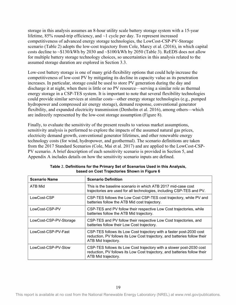
19 This report is available at no cost from the National Renewable Energy Laboratory (NREL) at www.nrel.gov/publications.

storage in this analysis assumes an 8-hour utility scale battery storage system with a 15-year lifetime, 85% round-trip efficiency, and ~1 cycle per day. To represent increased competitiveness of advanced energy storage technologies, the LowCost-CSP-PV-Storage scenario (Table 2) adopts the low-cost trajectory from Cole, Marcy et al. (2016), in which capital costs decline to ~$130/kWh by 2030 and ~$100/kWh by 2050 (Table 3). ReEDS does not allow for multiple battery storage technology choices, so uncertainties in this analysis related to the assumed storage duration are explored in Section 3.3.

Low-cost battery storage is one of many grid-flexibility options that could help increase the competitiveness of low-cost PV by mitigating its decline in capacity value as its penetration increases. In particular, storage could be used to store PV generation during the day and discharge it at night, when there is little or no PV resource—serving a similar role as thermal energy storage in a CSP-TES system. It is important to note that several flexibility technologies could provide similar services at similar costs—other energy storage technologies (e.g., pumped hydropower and compressed air energy storage), demand response, conventional generator flexibility, and expanded electricity transmission (Denholm et al. 2016), among others—which are indirectly represented by the low-cost storage assumption (Figure 8).

Finally, to evaluate the sensitivity of the present results to various market assumptions, sensitivity analysis is performed to explore the impacts of the assumed natural gas prices, electricity demand growth, conventional generator lifetimes, and other renewable energy technology costs (for wind, hydropower, and geothermal). The scenario definitions are taken from the 2017 Standard Scenarios (Cole, Mai et al. 2017) and are applied to the LowCost-CSP-PV scenario. A brief description of each sensitivity scenario is provided in Section 5, and Appendix A includes details on how the sensitivity scenario inputs are defined.

Table 2. Definitions for the Primary Set of Scenarios Used in this Analysis, based on Cost Trajectories Shown in Figure 6

Scenario Name Scenario Definition

ATB Mid This is the baseline scenario in which ATB 2017 mid-case cost trajectories are used for all technologies, including CSP-TES and PV.

LowCost-CSP CSP-TES follows the Low Cost CSP-TES cost trajectory, while PV and batteries follow the ATB Mid cost trajectory.

LowCost-CSP-PV CSP-TES and PV follow their respective Low Cost trajectories, while batteries follow the ATB Mid trajectory.

LowCost-CSP-PV-Storage CSP-TES and PV follow their respective Low Cost trajectories, and batteries follow their Low Cost trajectory.

LowCost-CSP-PV-Fast CSP-TES follows its Low Cost trajectory with a faster post-2030 cost reduction, PV follows its Low Cost trajectory, and batteries follow their ATB Mid trajectory.

LowCost-CSP-PV-Slow CSP-TES follows its Low Cost trajectory with a slower post-2030 cost reduction, PV follows its Low Cost trajectory, and batteries follow their ATB Mid trajectory.

20 This report is available at no cost from the National Renewable Energy Laboratory (NREL) at www.nrel.gov/publications.

Table 3. Solar Cost Inputs for the ATB Mid and Low-Cost Solar Trajectoriesa

2030 LCOE (¢/kWh)

2050 LCOE (¢/kWh)

Technology Scenario (CSP-TES) or Market Sector (PV)

Benchmark (Year) [¢/kWh]

ATB Mid LowCost ATB

Mid LowCost

CSP

-TES

LowCost-CSP 10.3 (2020) 8.8 5 7.8 4

LowCost-CSP-PV-Fast 10.3 (2020) 8.8 5 7.8 3.35

LowCost-CSP-PV-Slow 10.3 (2020) 8.8 5 7.8 4.75

PV

Utility-scale 7 (2016) 5.7 3 4.7 2

Commercial rooftop 13 (2016) 9.1 4 7.0 2.7

Residential rooftop 18 (2016) 10.2 5 8.3 3.3 a Corresponding values are shown for CSP-TES and utility-scale PV in Figure 6, and for commercial and residential rooftop PV in Appendix A. The LCOE in the table is calculated using the capacity factor that would be seen in Daggett, California, for CSP-TES, and in Kansas City, Missouri, for PV technologies. See Appendix A for details.

21 This report is available at no cost from the National Renewable Energy Laboratory (NREL) at www.nrel.gov/publications.

3 Solar Capacity and Generation in the Low-Cost Solar Scenarios

This analysis indicates that achieving the 2030 solar cost targets could lead to substantial growth in solar capacity countrywide (Figure 10). For all scenarios, new PV capacity represents most additions to the grid before 2030, most of which is deployed to satisfy capacity reserve requirements. It is interesting to note PV’s similar deployment levels in the baseline and LowCost-CSP scenarios, the latter of which includes a 15% reduction in cumulative PV capacity in the 2040s. The relative insensitivity of PV deployment to low-cost CSP-TES reflects the large magnitude and geographic extent of available resource for cost-effective PV—some of which lies in areas that are not considered for CSP-TES in this analysis (i.e., the pale-yellow shading in Figure 1)—even under the ATB Mid cost trajectory.

Figure 10. Cumulative capacity of CSP-TES (solid lines) and PV (dotted lines) for the baseline

(ATB Mid) and primary low-cost solar scenarios

By the mid-2020s, new PV capacity in the LowCost-CSP-PV and LowCost-CSP-PV-Storage scenarios begins to diverge from that in the baseline and LowCost-CSP scenarios (Figure 10). Acceleration in PV deployment in the former scenario reflects the impact of assumed cost reductions on the path toward the 2030 cost targets for PV, while the latter scenario is also impacted by the availability of low-cost battery storage (Figure 8), which helps mitigate the decline in PV’s capacity value as its penetration increases.

By contrast, CSP-TES capacity and generation only expand if the 2030 cost targets are realized, as depicted by the difference between the baseline and low-cost solar scenarios in Figure 10. In the low-cost solar scenarios, the first new CSP-TES installations come online in the late 2020s, when the demand for new capacity increases due to tightening reserve margins, and as the cost for CSP-TES begins to approach the 2030 cost target (Figure 8).

22 This report is available at no cost from the National Renewable Energy Laboratory (NREL) at www.nrel.gov/publications.

Countrywide, new CSP-TES deployment in the low-cost solar scenarios is approximately 1–2 GW per year in the late-2020s (Figure 11). This annual deployment rate is similar in magnitude to the cumulative CSP capacity in the United States to date, but it is well below the current rate of deployment for solar PV and other electricity generation technologies (EIA 2018a). New CSP-TES deployment remains below 2 GW per year throughout the analysis when a low-cost battery storage trajectory is assumed, but it grows steadily in the 2030s and beyond in the LowCost-CSP and LowCost-CSP-PV scenarios, eventually reaching 12–15 GW per year by 2050. This level of deployment is consistent with current and forecasted deployment rates for other generating technologies, such as natural gas combined cycle plants (NG-CC) (EIA 2018a). However, it is notably higher than historical deployment rates for CSP-TES, which highlights the need for a robust manufacturing and supply chain capability if the 2030 cost targets are achieved.

Figure 11. Annual net CSP-TES deployments for the baseline (ATB Mid) and primary low-cost

solar scenarios, with negative values indicating retirements of existing CSP-TES plants

The cumulative impact of these post-2030 deployment rates for CSP-TES is an increase in its share of total installed capacity and generation over time (Figure 12), particularly in the LowCost-CSP and LowCost-CSP-PV scenarios. Comparison of these two scenarios with the baseline scenario reveals that this deployment of CSP-TES capacity displaces similar amounts of natural gas-fired and wind capacity. Similar generator types are displaced in the LowCost-CSP-PV-Storage scenario, but this displacement is primarily due to increased PV and battery storage capacities (as opposed to CSP-TES capacity).

23 This report is available at no cost from the National Renewable Energy Laboratory (NREL) at www.nrel.gov/publications.

In the LowCost-CSP scenario, CSP-TES represents 10% of total capacity in the contiguous United States in 2050 (Figure 12), when its capacity has grown to 158 GW (Figure 10). For the LowCost-CSP-PV scenario, additional deployment of low-cost PV displaces some of the new CSP-TES capacity, which grows to 135 GW in 2050, or 7% of total capacity.29 Finally, assuming low-cost battery storage reduces cumulative CSP-TES deployment to 25 GW by 2050 in the LowCost-CSP-PV-Storage scenario (an 81% reduction relative to LowCost-CSP-PV). The lower deployment of CSP-TES under the assumption of low-cost battery storage suggests direct competition among solar technologies when low-cost storage is available for both PV and CSP.

This analysis further indicates that the amount of electricity generated by CSP-TES grows at a rate that is consistent with its growth in capacity (Figure 10, Figure 12). In the LowCost-CSP and LowCost-CSP-PV scenarios, growth in CSP-TES generation (and its share of total generation) begins slowly in about 2030 and accelerates after 2040, which is consistent with the rapid deployment of CSP-TES during this period. As a share of total generation, CSP-TES grows from less than 1% in 2030 to 5% in 2040, and it ultimately provides around 15% of total electricity generation in 2050 in the LowCost-CSP and LowCost-CSP-PV scenarios (Figure 12, Table 4). Finally, in the LowCost-CSP-PV-Storage scenario, the more limited growth in CSP-TES capacity results in slower growth in its share of generation, which reaches 3% by 2050.

29 The outsized decrease in CSP-TES’s share of capacity nationwide reflects the fact that total installed capacity in 2050 for the LowCost-CSP-PV scenario is approximately 25% higher than in the LowCost-CSP scenario, due to the lower capacity factor of PV relative to CSP-TES.

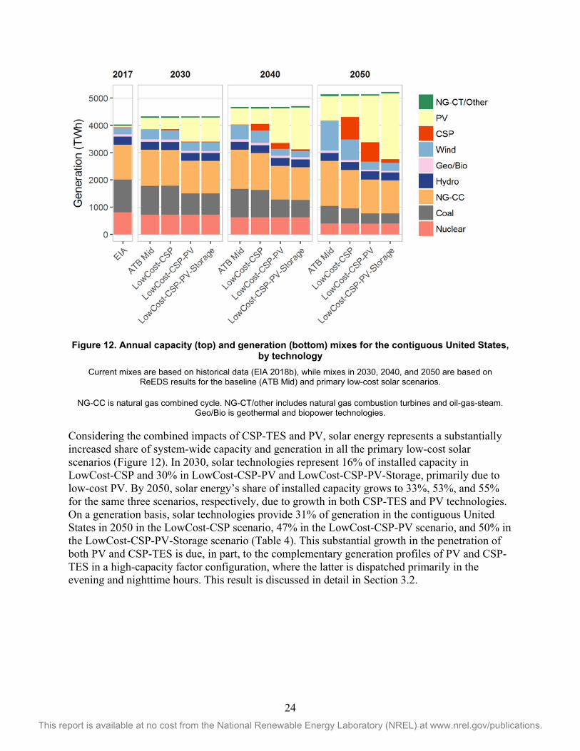
24 This report is available at no cost from the National Renewable Energy Laboratory (NREL) at www.nrel.gov/publications.

Figure 12. Annual capacity (top) and generation (bottom) mixes for the contiguous United States, by technology

Current mixes are based on historical data (EIA 2018b), while mixes in 2030, 2040, and 2050 are based on ReEDS results for the baseline (ATB Mid) and primary low-cost solar scenarios.

NG-CC is natural gas combined cycle. NG-CT/other includes natural gas combustion turbines and oil-gas-steam. Geo/Bio is geothermal and biopower technologies.

Considering the combined impacts of CSP-TES and PV, solar energy represents a substantially increased share of system-wide capacity and generation in all the primary low-cost solar scenarios (Figure 12). In 2030, solar technologies represent 16% of installed capacity in LowCost-CSP and 30% in LowCost-CSP-PV and LowCost-CSP-PV-Storage, primarily due to low-cost PV. By 2050, solar energy’s share of installed capacity grows to 33%, 53%, and 55% for the same three scenarios, respectively, due to growth in both CSP-TES and PV technologies. On a generation basis, solar technologies provide 31% of generation in the contiguous United States in 2050 in the LowCost-CSP scenario, 47% in the LowCost-CSP-PV scenario, and 50% in the LowCost-CSP-PV-Storage scenario (Table 4). This substantial growth in the penetration of both PV and CSP-TES is due, in part, to the complementary generation profiles of PV and CSP-TES in a high-capacity factor configuration, where the latter is dispatched primarily in the evening and nighttime hours. This result is discussed in detail in Section 3.2.

25 This report is available at no cost from the National Renewable Energy Laboratory (NREL) at www.nrel.gov/publications.

Table 4. Cumulative Capacities and Generation for Solar and Storage Technologies in 2030, 2040, and 2050 for the Baseline (ATB Mid)a and Primary Low-Cost Solar Scenarios

Capacity (GW)b Penetration (% of Generation)

Scenario Technology 2030 2040 2050 2030 2040 2050

ATB Mida

CSP-TES 1.9 1.9 0.5 0 0 0

PVc 220 319 489 10 13 18

Total solar 221 321 489 10 13 18

Battery storaged 0 0.8 2.8 0.0 0.0 0.1

LowCost-CSP

CSP-TES 7 46 158 1 5 16

PV 216 301 425 10 12 15

Total solar 223 346 582 10 17 31

Battery storage 0 0 0.5 0.0 0.0 0.0

LowCost-CSP-PV

CSP-TES 6 42 135 1 5 14

PV 469 720 1,020 20 27 33

Total solar 475 761 1,155 21 32 47

Battery storage 0 0 2 0.0 0.0 0.1

LowCost-CSP-PV-Storage

CSP-TES 6 13 25 1 1 3

PV 466 815 1,321 20 33 47

Total solar 472 828 1,346 21 34 50

Battery storage 5 73 199 0.3 3.4 9.2 a Values for the ATB Mid scenario are based on the 2017 ATB. b All capacities in this report are in terms of AC rather than DC. c Slight differences in reported values for PV compared to the Cole, Frew et al. (2017) are due to different ReEDS model versions used in each study. d The rows for battery storage show capacity and discharge from battery storage, but it does not include generation from other longer-duration storage systems, including pumped-hydropower and compressed air energy storage (e.g., pumped-hydro storage serves 0.4%–1.2% of load across all scenarios in 2050). Note that the penetration number for battery storage is calculated as total discharge divided by total load, and the actual energy is generated from other technologies.

It is interesting to note that PV penetration in 2050 is similar in the baseline and LowCost-CSP scenarios (Figure 12), which suggests limited competition between low-cost CSP-TES and mid-cost PV, which likely because of the different values provided by the technologies in the absence of low-cost battery storage as well as the different geographic footprints considered for each technology (Figure 1). By contrast, comparison of the LowCost-CSP-PV and LowCost-CSP-PV-Storage scenarios reveals slightly a 30% increase in PV capacity and a larger 42% increase in PV generation in the presence of low-cost battery storage.

26 This report is available at no cost from the National Renewable Energy Laboratory (NREL) at www.nrel.gov/publications.

Finally, within the context of the total generation mix (Figure 12) and relative to the baseline scenario, increased CSP-TES generation in the LowCost-CSP scenario largely displaces generation from NG-CC and wind generators. The combined impacts of low-cost PV and low-cost CSP-TES on the generation mix are more pronounced in the LowCost-CSP-PV and LowCost-CSP-PV-Storage scenarios, which include larger reductions in generation from multiple generator types.

3.1 Geographic Evolution of Solar Capacity This analysis indicates that achieving DOE’s 2030 cost targets for both CSP-TES and PV could result in solar capacity growth throughout the contiguous United States. The LowCost-CSP-PV scenario shows a net increase in solar capacity in every state by 2050 (Figure 13, page 27), with the most pronounced growth (relative to the baseline scenario) occurring in Texas and Florida as a results of a combination of new low-cost PV (primarily) and CSP-TES (secondarily). Incremental growth in solar capacity in the LowCost-CSP-PV scenario further indicates additional PV in many East North Central and mid-Atlantic states, many of which lie on the border of the available solar resource regions for CSP-TES in this analysis (Figure 1).

Comparison of the geographic distribution of new solar capacity in the LowCost-CSP scenario indicates a net 54 GW decrease in PV capacity, because decreases in PV capacity in the regions where solar resource is available for CSP-TES deployment outweigh the increases in PV capacity across much of the Northern half of the United States (Figure 14 [page 28]). Details of the evolution of utility-scale and distributed PV deployment that could result from achieving DOE’s 2030 cost targets for PV can be found in Cole, Frew et al. (2017). The remainder of this section provides a detailed discussion of the geographic and temporal evolution of CSP-TES systems in the LowCost-CSP and LowCost-CSP-PV scenarios.

Figure 13 shows the CSP-TES capacity by state for select years in the LowCost-CSP-PV scenario, and Figure 14 shows the corresponding difference in cumulative solar deployment in 2050 in the absence of low-cost PV (LowCost-CSP) and with the addition of low-cost battery storage (LowCost-CSP-PV-Storage). Across these three low-cost solar scenarios, the early state-level trends are similar and largely intuitive. For example, initial growth in low-cost CSP-TES capacity occurs in California, Arizona, and Nevada, which is consistent with historical builds for CSP. The next phase of CSP-TES deployment occurs in Texas (primarily in the higher-solar resource Texas Panhandle; see Figure 18, page 34), Colorado, and Kansas, but the timing of this phase varies across scenarios; deployment in these states occurs in the late 2030s and 2040s in the LowCost-CSP and LowCost-CSP-PV scenarios, but assuming low-cost battery storage delays deployment in similar locations until the late 2040s in LowCost-CSP-PV-Storage (Figure 13 and Figure 14).

27 This report is available at no cost from the National Renewable Energy Laboratory (NREL) at www.nrel.gov/publications.

Figure 13. CSP-TES (left) and PV (right) capacity (in GW) by state over time in the

LowCost-CSP-PV scenario

CSP-TES deployment remains restricted to the aforementioned states throughout the analysis period in the LowCost-CSP-PV-Storage scenario, but a key finding of this analysis is that achieving DOE’s 2030 cost target could lead to an expansion of the CSP-TES fleet into the Southeast and Midwest (Figure 14 and Figure 15, page 29). Deployment of CSP-TES in states along the Southern Atlantic coast in the late 2040s in the LowCost-CSP and LowCost-CSP-PV scenarios is somewhat counterintuitive, but it largely follows the magnitude of available CSP-TES capacity in these states (Figure 7, Table 1). Another important factor in the attractiveness of low-cost CSP-TES in these states is their ability to export electricity to other high-demand centers within the Eastern Interconnection—where electricity demand is more than three-times that of WECC—with high natural gas prices also playing an important role in Florida.

28 This report is available at no cost from the National Renewable Energy Laboratory (NREL) at www.nrel.gov/publications.

Figure 14. Maps showing the difference in cumulative CSP-TES (right) and PV (left) capacity

(in GW) in 2050 for the LowCost-CSP-PV-Storage (top) and LowCost-CSP (bottom) scenarios, relative to the LowCost-CSP-PV scenario (shown in Figure 13)

The same evolution of CSP-TES deployment in the LowCost-CSP-PV scenario is summarized in Figure 15, which breaks down the deployment by quality of solar resource. Assuming low-cost battery storage results in generally slower CSP-TES deployment (<2 GW per year), all of which is restricted to high- and mid-solar resource through 2050. In the absence of low-cost battery storage, new CSP-TES capacity in the mid-solar resource is delayed by a few years relative to deployment in the high-solar resource, but they eventually follow a similar growth trajectory through 2050. After DOE’s 2030 cost target has been achieved and additional learning further reduces costs (Figure 8), CSP-TES becomes cost-competitive in even low-solar resource classes (Figure 15). By the mid-2040s, deployment accelerates in low-solar resource classes, which ultimately host roughly one-third of cumulative CSP-TES capacity in 2050 in the primary low-cost solar scenarios without low-cost battery storage (Figure 16 [page 30]).

The sizable deployment of low-cost CSP-TES in the low-solar resource is largely counterintuitive, but it can be partly explained by the magnitude of available capacity within each class (Table 1) and the demand within each of the three asynchronous networks across the United States. On the former point, less than 2% of the available resource is deployed for each of the low- and mid-solar resource classes by 2050, compared to 16% in Class 12 (for both the LowCost-CSP-PV and LowCost-CSP scenarios respectively in the same year. To the latter point, CSP-TES capacity in the low-solar resource regions of the Eastern Interconnection in the absence of low-cost battery storage is not enough to compensate the higher demand in this network: on a generation basis, CSP-TES penetration is 24% and 29% in ERCOT and WECC in 2050, compared to 8% in the Eastern Interconnection in the LowCost-CSP-PV scenario.

29 This report is available at no cost from the National Renewable Energy Laboratory (NREL) at www.nrel.gov/publications.

CSP-TES Deployment in LowCost-CSP-PV

CSP-TES Deployment in LowCost-CSP-PV-Storage

Figure 15. Annual CSP-TES deployments for the LowCost-CSP-PV (top) and LowCost-CSP-PV-

Storage (bottom) scenarios, by quality of resource Definitions for High-, Mid-, and Low-solar resource follow Table 1. Note the different vertical scales. Deployment rates for the LowCost-CSP scenario are comparable to those in the top panel, but with accelerated deployment in the mid-

and low-solar resource regions after 2040.

30 This report is available at no cost from the National Renewable Energy Laboratory (NREL) at www.nrel.gov/publications.

Figure 16. Cumulative capacity of CSP-TES by resource class in 2050 for the LowCost-CSP

(bottom), LowCost-CSP-PV (middle), and LowCost-CSP-PV-Storage (top) scenarios Definitions for Low, Mid, and High follow Table 1.

Low is DNI < 6.25 kWh/m2/day. Mid is 6.25 ≤ DNI < 7.25. High is DNI ≥ 7.25.

It is important to emphasize that these results do not suggest that a lower-quality resource class is preferred over a higher-quality resource class if both are available in the same region. In fact, deployment of low-cost CSP-TES in the Southeast—driven by the aforementioned market factors—occurs in lowest-solar resource classes (Figure 17) because they are the only classes available in this analysis in that region (Figure 7). Moreover, Figure 17 demonstrates that while a wide array of solar resource quality (Classes 1–7) are available in Kansas, CSP-TES deployment in the state only occurs in Class 5 and above, with most deployment occurring in the highest resource classes that are available in a given region (Figure 17, Figure 7).

31 This report is available at no cost from the National Renewable Energy Laboratory (NREL) at www.nrel.gov/publications.

Figure 17. Cumulative CSP-TES capacity in 2050 for the LowCost-CSP-PV scenario,

by ReEDS model region and quality of solar resource

Despite these logical explanations of the model’s behavior, the cost-competitiveness of low-cost CSP-TES in multiple new states with low-solar resource is a unique finding of this analysis, and it is a result that warrants additional consideration. The expansion of CSP-TES into the Southeast has not been found in previous analyses (e.g., the SunShot Vision Study [DOE 2012]), in large part because CSP-TES deployment was not allowed in much of the Southeast, where previous

32 This report is available at no cost from the National Renewable Energy Laboratory (NREL) at www.nrel.gov/publications.

solar resource assessments indicated no suitable solar resource30 existed outside Florida. Also, land cover in the Southeast is heavily forested and weather hazards involving high winds exist in many states, which presents potential challenges for CSP-TES siting, permitting, and construction. This analysis has attempted to reflect some of these challenges by removing capital cost multipliers for CSP-TES in the Eastern Interconnection (which would normally result in reduced capital costs throughout the Southeast and Midwest), but additional exploration of these potential challenges associated with CSP-TES in new regions of the United States is needed but beyond the scope of this report.

Finally, in terms of cumulative deployment, CSP-TES capacity in California grows to 31 GW of CSP-TES capacity in LowCost-CSP, 25 GW in LowCost-CSP-PV, and 13 GW in LowCost-CSP-PV-Storage by 2050. Despite the somewhat lower solar resource in Texas, CSP-TES growth and cumulative capacity in the state are comparable to those of California in the LowCost-CSP and LowCost-CSP-PV scenarios. The substantial growth in CSP-TES in Texas is largely proportional to the state’s high electricity demand, which is assumed to grow by 43% over the course of the analysis period, resulting in larger capacity addition requirements than any other state.31 Another important factor is that the Texas Panhandle lies within the Eastern Interconnection—the demand in which is more than three-times that of WECC—which means CSP-TES deployed in the region can be exported to other high demand centers by leveraging the existing transmission network in that region. Finally, the inclusion of capital cost multipliers in Texas results in slightly lower capital costs than those in WECC, which increases the competitiveness of CSP-TES in the state. By contrast, assuming low-cost battery storage results in reduced CSP-TES capacity in Texas, which sees higher net value in the combination of low-cost PV and battery storage.

Somewhat surprisingly, achieving DOE’s 2030 solar cost targets leads to CSP-TES capacity in the high-solar resource states of Utah, New Mexico, and Nevada that is roughly 10%, 18%, and 19% that of California in the LowCost-CSP-PV scenario (and 10%, 16%, and 24% in the LowCost-CSP scenario) in 2050. The discrepancy is more pronounced when assuming low-cost battery storage, with cumulative capacity in 2050 in these three states reaching 1%–5% of new CSP-TES capacity in California in the LowCost-CSP-PV-Storage scenario. Across these primary low-cost solar scenarios, the lower deployment of CSP-TES in these states likely reflects their more limited electricity demand and the challenge of moving that power to demand centers in WECC, as well as competition among solar generating technologies. Despite the relatively low levels of deployment in these high-solar resource states, the CSP-TES share of total installed capacity within the footprint of WECC grows to 15% in 2050 for LowCost-CSP-PV and 21% for LowCost-CSP, where the latter reflects a lower total capacity when PV is displaced by low-cost CSP-TES in a high-capacity factor configuration (see Section 3.2). The LowCost-CSP-PV-Storage scenario shows the inverse result, with CSP-TES representing 5% of WECC capacity in 2050 due to lower CSP-TES deployment, higher PV deployment, and a higher total capacity than the LowCost-CSP-PV scenario.

30 A suitable solar resource for CSP-TES is defined here as average DNI of greater than 5 kWh/m2/day. 31 For comparison and context, Texas adds a similarly large amount of new natural gas-combined cycle capacity in both scenarios, despite the availability of low-cost solar systems.

33 This report is available at no cost from the National Renewable Energy Laboratory (NREL) at www.nrel.gov/publications.

3.2 The Value and Operation of Low-Cost Solar Capacity In evaluating the economics of new solar installations, one must consider both the costs and system-wide benefits associated with the technology. In particular, determining the net value depends on both the annualized costs of the system, as well as the economic value associated with providing energy (operational value) and firm capacity (capacity value) to the system. These values vary based on (1) the solar generating technology and its design parameters (e.g., Jorgenson et al. 2014 and Jorgenson et al. 2016) and (2) which generating technologies are being displaced by the solar technology.

This analysis assumes all new CSP-TES plants will be based on the molten-salt power tower technology, but the specific design parameters for CSP-TES—the solar multiple and duration of storage hours—are optimized in ReEDS for each plant. In particular, the model dynamically selects the combination of design parameters (solar multiple, storage duration, and turbine) for each CSP-TES plant in order to maximize its net value, based on the cost of building the plant relative to the value it can provide to the system. Based on the present representation of the 2030 cost targets—which involves 50%-80% cost reductions for the solar field and TES system—the optimal CSP-TES plant has a high capacity factor configuration, which enables dispatchable electricity by using high solar multiples and long-duration storage (Figure 18).32 This configuration is particularly pronounced in the low-solar resource regions of the Southeast and Midwest, where the optimal plants often adopt solar multiples and storage hours that approach the maxima allowed by the model, as described in Appendix C.33

According to observations of the existing fleet in the United States, estimates for the annual CSP capacity factors in 2016 range from 10% to 30% (Bolinger et al. 2017, Figure 26). This range represents different CSP technologies and lower-than-expected capacity factors for the newest CSP plants, many of which are still ramping up to their expected capacity factors due to early-stage operational challenges.34

Based on the optimal plant configuration, the annual capacity factors for the future CSP-TES fleet increase rapidly to a value around 60%, regardless of the solar resource class. It is worth noting that this annual value represents the average of the seasonal capacity factors—which range from approximately 45% in the winter to 70% in the summer (Appendix D)—weighted by the amount of CSP-TES generation in each season.

32 The ReEDS modeling in this analysis only represents CSP-TES plants with capacity factors larger than 40%, based on lower bounds for TES and solar multiples of six hours and 1.4–1.8, where the range reflects the different solar resource classes. As a result of these model constraints, this analysis does not fully evaluate the cost-effectiveness of peaker-type CSP-TES configurations. It is anticipated that future ReEDS analysis will modify this constraint to allow for a wider variety of CSP-TES configurations. 33 It is worth noting that the modeled least-cost configuration for CSP-TES is only partially consistent with the results of previous analyses. Using a production cost model to represent the California ISO with a 40% renewable portfolio standard, Jorgenson et al. (2014) found that the highest-value CSP-TES systems would have large thermal energy storage capacity, but they also found reduced value in large solar multiples. The discrepancy between their results and the present results could be due to the different geographic extents studied and/or the significantly reduced costs assumed in this analysis. 34 The corresponding values for the existing power-tower plants fall toward the lower end of this range (13%–20%) due to unplanned closures in their first years of operation. This range is also consistent with an approximate capacity factor for the entire CSP fleet of approximately 22%, based on historical data (EIA 2018b).

34 This report is available at no cost from the National Renewable Energy Laboratory (NREL) at www.nrel.gov/publications.

Figure 18. Histogram of the optimal design parameters for new CSP-TES installations by interconnect in the LowCost-CSP-PV scenario, which demonstrates the trend toward a

dispatchable, high-capacity factor configuration (with a high solar multiple and a long storage duration), particularly in the lower-solar resource regions within the Eastern interconnection

As previously mentioned, the specific design parameters for CSP-TES were optimized in ReEDS to maximize the net value of the system. The annualized costs of such a plant follow directly from the representation of the 2030 cost targets for CSP-TES in this analysis. The breakdown of revenue provided to new CSP-TES plants provides some insights into the value associated with this preferred plant design, which derives most of its revenue from energy (operational) services (60%–80%, depending on the year and scenario), as opposed to capacity services. These relative shares of energy and capacity value for new CSP-TES are the inverse of what has been found in previous analyses; for example, Jorgenson et al. (2014) evaluated the value streams for new CSP-TES in the southwestern region of WECC and found that more than half of CSP-TES’s value was derived from its ability to provide firm capacity. The current result differs, at least in part, because it is evaluating the impacts of a 50% reduction in solar LCOE’s by 2030, which places downward pressure on capacity prices going forward. In addition, the national scale of the present modeling reflects regional capacity values from across the United States, whereas the scope in Jorgenson et al. (2014) only included capacity values in the Southwest.

Figure 19 shows the average dispatch (operation) patterns of the system in 2050 for the LowCost-CSP and LowCost-CSP-PV scenarios, which demonstrate the energy value that is provided to new CSP-TES plants. In the former scenario, CSP-TES generation levels are highest during the evening and overnight hours (5 p.m. to 6 a.m.), in terms of both absolute generation and share of total generation (17%–26%). During these times, CSP-TES is primarily displacing generation from wind and natural gas systems, relative to the baseline scenario (not shown). CSP-TES also provides a limited amount of generation during the daytime hours (6 a.m. to 5 p.m.) in this scenario, when it displaces minor amounts of solar and wind generation (relative to the baseline scenario) and provides up to 17% of total generation.

35 This report is available at no cost from the National Renewable Energy Laboratory (NREL) at www.nrel.gov/publications.

Figure 19. Dispatch stack for four representative days in 2050 for the LowCost-CSP-PV (top) and

LowCost-CSP (bottom) scenarios NG-CC is natural gas combined cycle. NG-CT/other includes natural gas combustion turbines and oil-gas-steam.

Geo/Bio is geothermal and biopower technologies.

In the LowCost-CSP-PV scenario, CSP-TES behaves in a similar fashion but with more pronounced differences in its generation levels during the daytime and nighttime hours (Figure 19). CSP-TES is the primary energy supplier during the evening and nighttime hours (5 p.m. to 6 a.m.) throughout the year, when it provides 18%–30% of electricity generation. CSP-TES generation is much more limited in the early morning (3%–10%) and afternoon (0%–6%) hours. This profile mirrors that of low-cost PV, which is the primary energy supplier during daytime hours (6 a.m. to 5 p.m.) in this scenario. The complementary nature of the CSP-TES and PV generation profiles highlights the importance of thermal energy storage for CSP-TES, which provides both flexibility and dispatchable generation when the sun is down. These attributes also help explain why CSP-TES largely displaces natural-gas fired generation, which currently operates in a similar manner as the modeled generation profile for CSP-TES (Figure 19). Nuclear and coal generators operate in a typical baseload fashion in summer and winter in this scenario, but the latter ramps down during the spring to its minimum generation levels.

36 This report is available at no cost from the National Renewable Energy Laboratory (NREL) at www.nrel.gov/publications.

Figure 20 shows the difference between the dispatch patterns for low-cost solar in the absence (LowCost-CSP-PV) and presence (LowCost-CSP-PV-Storage) of low-cost battery storage. In the figure, positive PV and storage values correspond to increased generation from these systems, and negative storage values correspond to the charging of the batteries in the LowCost-CSP-PV-Storage scenario. The negative CSP-TES values indicate that the addition of low-cost battery storage primarily displaces generation from CSP-TES, with more minor reductions from NG-CC plants. The more direct competition between low-cost CSP-TES and the combination of low-cost PV and battery storage likely reflects both their overlapping resource and services provided to the grid.

Figure 20. The difference in the average dispatch stack for four representative days (in 2050)

between the LowCost-CSP-PV and LowCost-CSP-PV-Storage scenarios

It is interesting to note that the average dispatch (operation) of the system in 2050 varies by region and trends closely follow the quality of solar resource (Figure 21).35 In the absence of low-cost battery storage, PV provides the bulk of solar generation during the daytime hours in all North American Electric Reliability Corporation (NERC) regions, while CSP-TES generation is concentrated in the evening and overnight hours, as previously described. However, in the NERC regions that roughly correspond to the high- (California and Colorado/Arizona/New Mexico, represented by RA) and mid-solar resource regions (ERCOT, Southwest Power Pool), CSP-TES

35 NERC regions that are not included—East Central Area Reliability Coordination Agreement (ECAR), Mid-Atlantic Area Council (MAAC), Mid America Interconnected Network (MAIN), New York (NY), and New England (NE)—represent regions where CSP-TES is not deployed by 2050, primarily due to a lack of suitable resource (DNI ≥ 5 kWh/m2/day in this analysis).

37 This report is available at no cost from the National Renewable Energy Laboratory (NREL) at www.nrel.gov/publications.

also provides a notable amount of generation in both the morning and afternoon “timeslices,” on a percentage basis. This daytime CSP-TES generation likely reflects the optimal system design in these regions—which includes slightly lower solar multiples and hours of storage duration (Figure 18)—as well as their relatively high daytime electricity demand. Altogether, solar resources represent approximately 75% of the total generation in these high-solar resource NERC regions in the LowCost-CSP-PV scenario, divided evenly between CSP and PV (Figure 21). Solar’s share of total generation is around 70% in the LowCost-CSP and LowCost-CSP-PV-Storage scenarios, where the former is dominated by generation from CSP-TES and the latter by generation from PV.

Figure 21. Dispatch stack (on a percentage basis) for four representative days in 2050 for each

NERC region in which CSP-TES is deployed in the LowCost-CSP-PV scenario Similar patterns are observed in the LowCost-CSP scenario, whereas CSP-TES generation is limited to only the high-

and mid-solar resource regions (i.e., the top panel of the figure) in the LowCost-CSP-PV-Storage scenario.

NG-CC is natural gas combined cycle. NG-CT/other includes natural gas combustion turbines and oil-gas-steam. Geo/Bio is geothermal and biopower technologies.

38 This report is available at no cost from the National Renewable Energy Laboratory (NREL) at www.nrel.gov/publications.

By contrast, CSP-TES provides very little daytime generation in the NERC regions that lie exclusively in the low-solar resource regions36 (e.g., the SERC Reliability Corporation region [SERC], Florida [FL], and Mid-Continent Area Power Pool [MAPP]), where the optimal system is designed to store solar energy to dispatch in the evening and overnight hours. This analysis also indicates widespread deployment of PV capacity in these regions, which might be driving CSP-TES generation to hours when solar resource is unavailable. Altogether, solar resources represent 21%–54% of generation in these low-solar resource NERC regions (Figure 21), most of which comes from PV. Solar’s share of generation in these regions is similar in the LowCost-CSP-PV-Storage scenario (all of which comes from PV), but solar’s share declines to 5%–42% of generation in these regions in the LowCost-CSP scenario, less than half of which comes from CSP-TES.

Finally, Figure 22 shows the impact of low-cost solar systems on curtailment rates—defined here as curtailments divided by variable renewable energy generation—in the contiguous U.S. electricity system. It is important to note that CSP-TES configuration constraints in ReEDS are designed to avoid curtailment from these systems, so the impacts shown in Figure 22 reflect changes to the curtailment and overall generation levels from variable PV and wind.

Despite similar levels of PV penetration (Table 4), the 2050 curtailment rate in LowCost-CSP is approximately half that in the baseline scenario (1.1% compared to 2.2% in 2050). The reduced curtailment rate in LowCost-CSP reflects both the displacement of variable renewable generation by CSP-TES, as well as the increased flexibility that CSP-TES provides to the system. By contrast, the increased flexibility from CSP-TES is not sufficient to compensate for a near-tripling of PV generation (relative to the baseline scenarios), the lack of transmission expansion (particularly in the Southeast), and the lack of cost-competitive battery storage systems in the LowCost-CSP-PV scenario, the combination of which results in a curtailment rate that grows to 9.6% by 2050 in the LowCost-CSP-PV scenario. The assumption of low-cost battery storage helps mitigate some of the cost-effective “throwing away” of energy in the LowCost-CSP-PV-Storage scenario, where the curtailment rate of 3.5% in 2050 is closer to the baseline and LowCost-CSP scenarios because of the increased system flexibility provided by both low-cost CSP-TES and battery storage in this scenario.

36 It is worth noting that the Northwest Power Pool (NWP) region contains a wide range of solar resource and the corresponding dispatch pattern closely resembles that of the low-solar resource regions, likely due to the larger installed capacity in those portions of the region.

39 This report is available at no cost from the National Renewable Energy Laboratory (NREL) at www.nrel.gov/publications.

Figure 22. The modeled curtailment rate, defined as curtailment divided by variable renewable

energy generation, for the baseline (ATB Mid) and primary low-cost solar scenarios

3.3 Uncertainties Related to Input Assumptions Beyond the inherent challenges associated with modeling the future of the complex electricity system in the contiguous United States, there are many other input assumptions that introduce varying levels of uncertainty into the model results. Multiple examples are mentioned throughout this report, but it is impossible to test all sources of uncertainty. Here we discuss the source, direction, and relative magnitude of some of the most prominent uncertainties related to a variety of assumptions that have been quantitatively tested in the model through sensitivities around select low-cost solar scenarios, including the assumed post-2030 cost reductions for CSP-TES, ability to build new transmission, duration for battery storage technologies, and regional cost multipliers for CSP-TES.

3.3.1 Post-2030 Cost Trajectory for CSP-TES This section explores the sensitivity of the previously described results to two different post-2030 cost trajectories for CSP-TES (Figure 23 [page 40]). Both cost sensitivity scenarios achieve the 2030 solar cost targets, but LowCost-CSP-PV-Slow and LowCost-CSP-PV-Fast are defined by 5% and 33% cost reductions, respectively, for CSP-TES between 2030 and 2050. Both cost sensitivity scenarios assume a 33% reduction for PV over the same period, to maintain consistency with Cole, Frew et al. (2017).

The cumulative capacity (Figure 23) and deployment patterns (Figure 24 [page 42] and Figure 25 [page 44]) for CSP-TES depend on the assumed post-2030 cost reductions, which indicates that CSP-TES is likely on the margin throughout the analysis period. The assumption of a 5% post-2030 cost reduction for CSP-TES in LowCost-CSP-PV-Slow results in a more limited deployment pattern for CSP-TES (Figure 24 and Figure 25), which resembles the LowCost-CSP-PV-Storage scenario in geographic extent and magnitude. In particular, most new CSP-TES is deployed in the high- and mid-solar resource regions, with limited deployment in Class 3 (low)

40 This report is available at no cost from the National Renewable Energy Laboratory (NREL) at www.nrel.gov/publications.

solar resource in Florida in the mid-2040s. The high-solar resource regions are less sensitive to the 5% post-2030 cost trajectory, such that their cumulative installed capacity is reduced by 10% in 2050, with impacts on deployment in the mid-solar resource regions falling somewhere in between. Cumulative CSP-TES capacity in this scenario is 67 GW in 2050, or 50% lower than in the LowCost-CSP-PV scenario.

The assumption of a 33% post-2030 cost reduction for CSP-TES in the LowCost-CSP-PV-Fast scenario has an inverse affect, with accelerated growth in CSP-TES deployment in the low-solar resource regions occurring after 2040 (Figure 25). As a result, cumulative CSP-TES capacity grows by to 198 GW in 2050, roughly half of which is hosted in the low-solar resource regions.37 Minor amounts of new CSP-TES also emerge toward the end of the analysis period in new low-solar resource states, including Arkansas, Montana, Idaho, and North Dakota.

Figure 23. The impact of assuming different post-2030 cost trajectories for CSP-TES

on cumulative CSP-TES capacity, nationwide The lower bound, solid red curve, and upper bound reflect cost reductions for CSP-TES of 5%, 20% and 33%,

respectively, between 2030 and 2050.

37 For comparison, recall that CSP-TES deployment in LowCost-CSP-PV was 135 GW in 2050, roughly one-third of which was hosted in the low-solar resource regions.

41 This report is available at no cost from the National Renewable Energy Laboratory (NREL) at www.nrel.gov/publications.

Figure 24. Maps showing the difference in cumulative CSP-TES (right) and PV (left) capacity (in GW) in 2050 for the LowCost-CSP-PV-Slow (top) and LowCost-CSP-PV-Fast (bottom)

scenarios, relative to LowCost-CSP-PV (shown in Figure 13)

42 This report is available at no cost from the National Renewable Energy Laboratory (NREL) at www.nrel.gov/publications.

Figure 25. Comparison of the cumulative capacity of CSP-TES by resource class in 2050 for the

LowCost-CSP-PV-Slow (top), LowCost-CSP-PV (middle), and LowCost-CSP-PV-Fast (bottom) scenarios

Definitions for Low, Mid, and High follow Table 1. Low is DNI < 6.25 kWh/m2/day. Mid is 6.25 ≤ DNI < 7.25. High is DNI ≥ 7.25.

Finally, it is interesting to note that deployment of PV in these post-2030 CSP-TES cost reduction sensitivity scenarios—which include the same post-2030 cost trajectory for PV—is largely insensitive to the post-2030 cost trajectory for CSP-TES. This result indicates that achieving the 2030 cost targets for PV would likely make it one of the lowest-cost generators, independent of the cost trajectory for CSP-TES.

43 This report is available at no cost from the National Renewable Energy Laboratory (NREL) at www.nrel.gov/publications.

3.3.2 New Transmission Availability The aforementioned capacity and generation results are based on the default ReEDS assumptions about the cost and availability of building new transmission to bring somewhat-remote solar generation to demand centers. Details of the transmission capacity requirements are discussed in Section 4.1, but this section presents the sensitivity of the aforementioned capacity and generation results to the assumption that new long-distance transmission capacity can be built. In particular, ReEDS has the option of disallowing new transmission capacity between balancing areas (e.g., Figure 53); with this option, new transmission spur lines can still be built within a given balancing area to connect remote generating capacity to the existing transmission infrastructure but only if sufficient transmission capacity is available within the existing network to move the new generation to demand centers.

To test the sensitivity of the previously described capacity and generation results to transmission restrictions, the three primary low-cost solar scenarios were rerun without the ability to build new transmission between balancing areas. The impacts of this assumption for each scenario are detailed below, but it is interesting to note that despite a sizable reduction in new transmission capacity (see Section 4.1), solar still represents a substantial fraction of new capacity and generation throughout the low-cost solar scenarios, which is achieved primarily by building new solar plants closer to the existing transmission network and/or demand centers.

In the LowCost-CSP scenario, disallowing new transmission resulted in slightly reduced CSP-TES capacity in the high- and mid-solar resource states that require new transmission capacity to be connected to high-demand centers (e.g., Arizona, New Mexico, and the central United States). This reduced CSP-TES deployment was partially offset by increased CSP-TES capacity in the lower-solar resource regions that have access to available capacity on the existing transmission network, but the net result was a 2 GW (1%) reduction in CSP-TES capacity by 2050. By contrast, disallowing new transmission between balancing areas increased cumulative PV deployment by 11 GW (or 3%), primarily because of the reduced deployment of remote wind capacity in the remote high-quality wind resource regions. When new transmission is disallowed in the scenario that assumed the low-cost trajectory for both solar technologies (LowCost-CSP-PV), minor reductions in both CSP-TES and PV capacity were observed relative to the scenario with default transmission assumptions.

Finally, in the scenario that assumes a low-cost trajectory for CSP-TES, PV, and battery storage, disallowing new transmission between balancing areas resulted in CSP-TES capacity that was increased by 1 GW in WECC, with a similar decrease in ERCOT. However, the impact on PV and battery storage deployment was more pronounced, with a 27 GW increase in PV and a 21 GW increase in battery storage capacity. The additional PV and battery capacities were concentrated in California, Texas, and the Southeast, with corresponding decreases in neighboring states (that would require new long-distance transmission to bring the corresponding generation to demand centers). The increased competitiveness of PV and battery storage likely reflects the synergies between these systems, as well as a higher net value for low-cost battery storage due to its flexibility in deployment location.

44 This report is available at no cost from the National Renewable Energy Laboratory (NREL) at www.nrel.gov/publications.

3.3.3 Battery Storage Duration As previously mentioned, ReEDS chooses the optimal design parameters (solar multiple, duration of storage hours, and turbine capacity) for each CSP-TES in order to maximize its net value, based on the cost of building the plant relative to the value it can provide to the system. Because ReEDS is a linear model, possible plant configurations are restricted to those with a linear relationship between solar field size, thermal storage capacity, and plant capacity factor.

However, ReEDS is currently unable to optimize battery storage system configurations, and it instead considers only one battery storage configuration in each model run. This analysis relies primarily on an assumption of eight-hour battery storage, which has the advantage of receiving nearly full capacity credit due to the longer-storage duration. However, the capital cost for an eight-hour system is higher than that of a shorter duration system, which could introduce a disadvantage for battery storage systems in the previously presented scenarios.

To test whether the assumed battery storage system impacts the relative competitiveness of CSP-TES versus battery storage, the three primary low-cost solar scenarios were rerun assuming a four-hour battery storage system (Figure 26), which has a lower capital cost and a slightly reduced capacity credit (75%). Under the assumptions of the LowCost-CSP and LowCost-CSP-PV scenarios, assuming a four-hour battery storage system resulted in 1–2 GW changes in CSP-TES and PV deployment, most of which occurred in Texas and along the Atlantic coast. Assuming a four-hour battery storage system also resulted in increased storage capacity deployment (4–7 GW), most of which was concentrated in the same regions and in PJM territory but less storage energy deployment (because the storage capacity is four-hour rather than eight-hour storage).

Figure 26. Impacts of the assumed battery system configuration (solid lines = four-hour, dashed lines = eight-hour) on the installed capacities of CSP-TES, PV, and storage in the three primary

low-cost solar scenarios

Switching to a four-hour battery storage system had a more pronounced impact under the assumption of low-cost battery storage (LowCost-CSP-PV-Storage). In particular, assuming four-hour battery storage reduced PV deployment throughout most of the country, such that cumulative PV deployment was decreased by 66 GW in 2050 (-8%). By contrast, battery storage capacity increased in nearly every state, with cumulative battery storage capacity increasing by

45 This report is available at no cost from the National Renewable Energy Laboratory (NREL) at www.nrel.gov/publications.

87 GW (40%), but overall generation discharge from battery storage decreasing by 26%. Finally, CSP-TES capacity was slightly increased in Colorado, Arizona, and New Mexico, but corresponding decreases in Colorado and Texas resulted in cumulative CSP-TES capacity that was largely unchanged from the underlying scenario (which includes 25 GW of CSP-TES capacity by 2050).

3.3.4 Regional Capital Cost Multipliers Capacity expansion models typically employ regional capital cost multipliers to reflect differences in the labor wage and productivity, seismic design, and owner costs, as well as remote location issues, location adjustments, and increased overheads. In general, such regional capital cost multipliers for solar technologies generally result in higher assumed capital costs along the West Coast and in the Northeast, and lower capital costs in the Gulf States and along the South Atlantic coast.

This analysis uses such capital cost multipliers for PV throughout the contiguous United States (see Appendix A), and for CSP-TES in WECC and ERCOT. However, the aforementioned results do not include any capital cost multipliers for the Eastern Interconnection, which would normally result in reduced capital costs for CSP-TES throughout the Southeast and Midwest (based on the capital cost multipliers for PV presented in Appendix A). Removing these multipliers was meant to reflect the potential for increased costs associated with land acquisition in this region, where multiple private landowners in the would likely be involved in a single CSP-TES project.

To test the impact of this assumption on the aforementioned results, the three primary low-cost solar scenarios were rerun with the PV capital cost multipliers applied to new CSP-TES projects throughout the contiguous United States (Figure 27). Implementing the regional capital cost multipliers for CSP-TES in the Eastern Interconnection had a negligible impact on the scenario that assumed a low-cost trajectory for CSP-TES, PV, and battery storage technologies (LowCost-CSP-PV-Storage). The relative insensitivity of this scenario likely reflects the limited competition between the solar generators in this scenario, as the model already saw a higher net value in the combination of low-cost PV and battery storage (rather than low-cost CSP-TES) in the Southeast, even in the absence of the regional capital cost multipliers for CSP-TES.

By contrast, this assumption had a sizable impact on the low-cost solar scenarios that do not assume low-cost battery storage. Specifically, implementing the regional capital cost multipliers for CSP-TES in the Eastern Interconnection resulted in a 25% increase in CSP-TES capacity in both the LowCost-CSP and LowCost-CSP-PV scenarios. Unsurprisingly, most of this growth in CSP-TES occurred in the Eastern Interconnection—with corresponding reductions primarily from natural-gas fired capacity in this region—and the most substantial CSP-TES expansion was concentrated in the southeastern states that have high natural gas prices (e.g., Florida) or the smallest (i.e., most impactful) regional capital cost multipliers, including South Carolina, Georgia, and Louisiana.

46 This report is available at no cost from the National Renewable Energy Laboratory (NREL) at www.nrel.gov/publications.

Figure 27. Modeled impact of implementing the PV-based capital cost multipliers in the Eastern Interconnection on PV (left) and CSP-TES (right) deployment in the three primary low-cost

solar scenarios Red (blue) values indicate additional (reduced) capacity when the regional capital cost multipliers are applied to CSP-

TES in the Eastern Interconnection. Note that the Texas Panhandle is part of the Eastern Interconnection.

47 This report is available at no cost from the National Renewable Energy Laboratory (NREL) at www.nrel.gov/publications.

4 Select Impacts of Low-Cost Solar This section explores select impacts of low-cost solar power on the U.S. electricity sector and the natural environment. In particular, the following subsections report transmission requirements and power flows, electricity prices and system costs, and impacts related to the environment. The results presented in the following subsections are focused on the LowCost-CSP-PV and LowCost-CSP scenarios. However, the corresponding results for the sensitivity scenarios typically scale with the extent of CSP-TES deployment, unless otherwise noted.

4.1 Transmission Requirements and Power Flows Due to the locations of high-quality solar resource, new transmission capacity38 is typically required to transport solar generation to demand centers. Figure 28 (page 48) shows that while this trend does hold in this analysis—with cumulative transmission in the low-cost solar scenarios lying above that of the baseline scenario—the incremental increase in transmission capacity required to bring substantial amounts of solar generation to demand centers is relatively minor. Across all scenarios, the incremental increase in transmission capacity is typically 2%–4% higher than the baseline scenario, which corresponds to a ~16% increase in transmission capacity compared to current levels. Scenarios with increased solar and/or wind capacity tend to require more transmission, but incremental increases remain below 6% in most scenarios.

The LowCost-CSP scenario suggests a negligible (0.1%) increase in transmission capacity relative to the baseline scenario through 2040. By 2050, the cumulative transmission capacity in the LowCost-CSP scenario is 3.1% higher than the baseline scenario (or 16% higher than 2016 levels). The incremental increase in transmission is more pronounced when assuming the low-cost trajectories for PV (LowCost-CSP-PV) and battery storage (LowCost-CSP-PV-Storage) systems. These scenarios indicate similar trajectories for new transmission capacity, including a near-term increase in transmission of 0.5% in 2030 and 1.2%–3.2% in 2040 (compared to the baseline scenario); this is primarily due to the earlier deployment of low-cost PV in these scenarios (Figure 29). This result also reflects the fact that achieving DOE’s 2030 cost target for CSP-TES can facilitate the deployment of this technology in locations that are closer to demand centers or existing transmission capacity. For example, Figure 29 shows that the LowCost-CSP scenario can achieve a similar level of CSP-TES penetration with a lower amount of cumulative transmission (in units of gigawatt-miles) than is required in the LowCost-CSP-PV scenario, despite the similar deployment pattern for CSP-TES in both scenarios (Figure 10). Moreover, the terminal transmission capacity requirements as a function of CSP-TES penetration are nearly identical in the LowCost-CSP and LowCost-CSP-PV scenarios, despite the increased CSP-TES penetration in the former scenario (16% compared to 14%). Finally, the pink curve in Figure 29 indicates that the similar solar penetration observed in the LowCost-CSP-PV-Storage scenario (relative to LowCost-CSP-PV) requires more transmission than the low-cost solar scenarios that do not assume the low-cost trajectory for battery storage technologies.

38 In this section, transmission capacity refers to high-voltage bulk power system transmission. It does not include the spur lines built to connect remote sites to the high-voltage transmission system or any distribution-level transmission.

48 This report is available at no cost from the National Renewable Energy Laboratory (NREL) at www.nrel.gov/publications.

Figure 28. Cumulative transmission capacity in units of GW-miles for the baseline (ATB Mid) and

primary low-cost solar scenarios

Figure 29. Transmission builds as a function of CSP-TES penetration (fraction of generation

supplied by CSP-TES) for the LowCost-CSP (orange), LowCost-CSP-PV (red), and LowCost-CSP- PV-Storage (pink) scenarios, where the vertical nature of the latter scenario reflects substantial transmission capacity

additions due to increased PV deployment (as opposed to increased CSP-TES deployment).

49 This report is available at no cost from the National Renewable Energy Laboratory (NREL) at www.nrel.gov/publications.

The geographic distribution of this additional transmission capacity demonstrates that it is primarily used to move low-cost generation from CSP-TES to high-demand centers. Figure 30 shows incremental growth in transmission capacity after 2010 in the baseline (ATB Mid) scenario, with additional maps showing the differences in 2050 transmission capacity in the LowCost-CSP, LowCost-CSP-PV, and LowCost-CSP-PV-Storage scenarios. All low-cost solar scenarios indicate transmission capacity increases in Texas—home to the largest cumulative capacity of both utility-scale PV and CSP-TES in 2050—which helps transport solar generation both within the state and to the Eastern Interconnection. In addition, increased transmission capacity to the north from North Carolina, and to the east from Kansas helps transport low-cost solar generation from the Southeast to the high-demand centers in the Northeast. Finally, reductions in transmission capacity in the Northwest reflect the capacity that is displaced by low-cost solar in these scenarios.

Notable differences between the scenarios exist in the Midwest and Southeast, which increased transmission capacity requirements in the LowCost-CSP and LowCost-CSP-PV scenarios respectively. Decreases in transmission capacity near Iowa in the LowCost-CSP-PV and LowCost-CSP-PV-Storage scenarios reflects the displacement of low-cost wind by low-cost PV and storage, whereas increases in this region in LowCost-CSP reflects increased generation from this high-quality wind resource. There is very little CSP-TES resource in the upper Midwest (which falls close to the lower-bound of 5.0 kWh/m2/day), so additional wind resources are built out in this region to supply the midwestern load centers in the LowCost-CSP scenario. Similarly, the increase in transmission capacity in Georgia in the LowCost-CSP-PV and LowCost-CSP-PV-Storage scenarios helps transport additional generation from low-cost PV in Georgia and Florida to the Northeast.

Figure 30. New transmission capacity from 2010 to 2050 for the baseline (ATB Mid) scenario (top left), with difference maps presenting the relative changes in 2050 transmission capacity for the

low-cost solar scenarios

50 This report is available at no cost from the National Renewable Energy Laboratory (NREL) at www.nrel.gov/publications.

Similar trends are apparent in the net imports maps (Figure 31), which show that Iowa and South Carolina are net exporters of generation in both scenarios. Higher levels of exports from Iowa in the LowCost-CSP scenario (relative to LowCost-CSP-PV) reflect its increased wind generation, whereas higher levels of exports from South Carolina in the LowCost-CSP-PV and LowCost-CSP-PV-Storage scenarios reflect increased generation from PV and CSP-TES, which is exported to neighboring states and beyond. A related impact of the reversal of the net power flows for Ohio and Virginia, which are directly impacted by the previously described increases in Iowa and South Carolina respectively.

Figure 31. Net electricity imports (purple) and exports (red) in 2050 by state for the low-cost

solar scenarios Values are presented in terawatt-hours (TWh).

4.2 Electricity Prices and System Costs This analysis suggests that cost reductions for solar generating technologies could lead to reductions in total system costs by 2050. Figure 32 shows system costs for the baseline and primary low-cost solar scenarios, where the most prominent cost categories are conventional fuel and O&M costs, followed by renewable and conventional capital costs, with transmission representing a narrow segment at the bottom of the stack. Comparison of the LowCost-CSP and the baseline reveals slight increases in renewable capital costs offsetting similar reductions in conventional fuel costs, along with slight reductions in conventional capital costs. These reductions primarily reflect the flexible nature of CSP-TES, which allows it to provide some peaking services and, in turn, reduces the need for peaking units (e.g., the reduction in natural gas combustion turbine capacity in Figure 12). The net result is a more cost-efficient system, with cost savings of $20 billion (2016–2050) relative to the baseline scenario.

Considering the combined effects of low-cost CSP-TES and PV, the relative changes between the LowCost-CSP-PV and baseline scenarios reflect a more pronounced transition from conventional generating sources toward solar generation sources, with larger decreases in conventional fuel, O&M, and capital costs. The net result for the LowCost-CSP-PV scenario is cumulative system-wide savings of $169 billion, primarily due to the avoided conventional fuel and O&M costs (Figure 32). Finally, system cost savings in the LowCost-CSP-PV-Storage scenario grow to $224 billion due to the further reduction in conventional capital costs.

51 This report is available at no cost from the National Renewable Energy Laboratory (NREL) at www.nrel.gov/publications.

Figure 32. Total present value of system costs from 2016 to 2050 for the baseline (ATB Mid) and

primary low-cost solar scenarios

Finally, analysis of wholesale electricity prices indicates that achieving DOE’s 2030 solar cost targets could help mitigate some of the electricity price increases evaluated in the baseline scenario (Figure 33). The specific contributions of CSP-TES can be seen in the comparison of the baseline and LowCost-CSP scenarios, where the latter’s electricity prices are slightly lower than the baseline beginning in 2030, shortly after the first new CSP-TES is deployed. The savings continue to increase throughout the analysis period due to relatively flat prices in the LowCost-CSP scenario after 2030, which results in electricity prices in 2050 that are 17% lower than in the baseline scenario. The LowCost-CSP-PV and LowCost-CSP-PV-Storage scenarios indicate similar impacts on electricity prices, including earlier (left panel) and deeper (right panel) electricity price savings that are due to the rapid deployment of low-cost PV; in these scenarios, the cumulative impact is 2050 electricity prices that are 21% lower than in the baseline scenario.

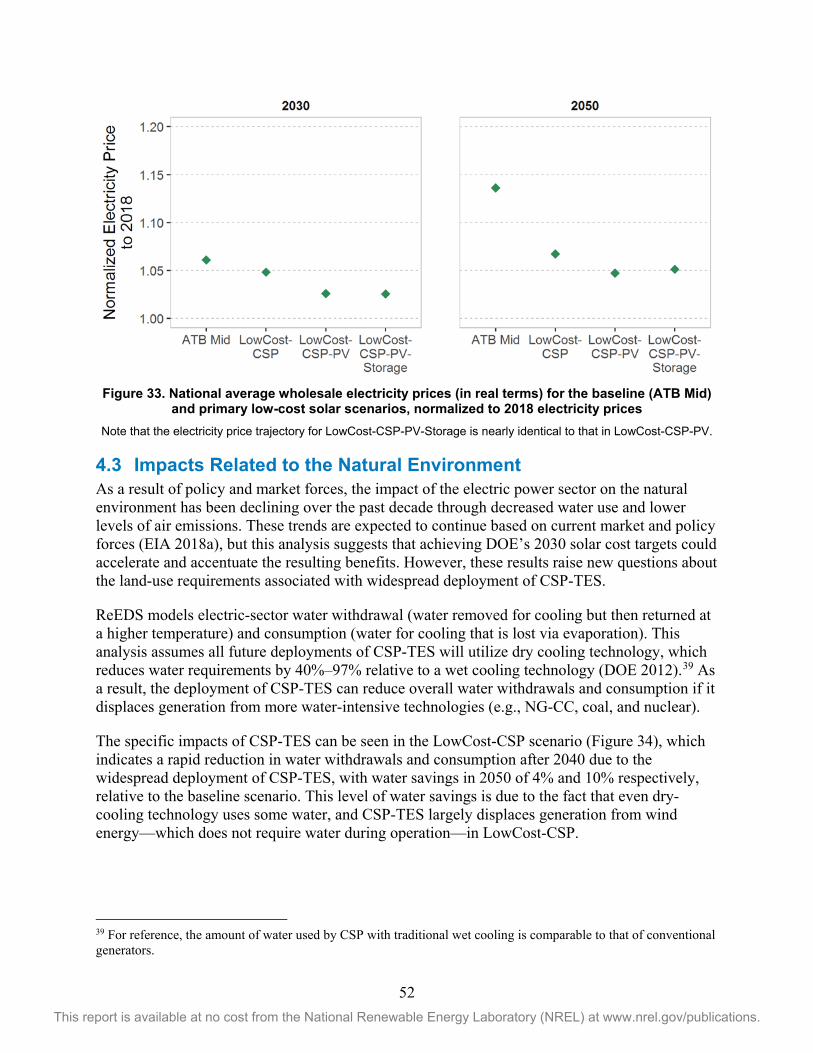
52 This report is available at no cost from the National Renewable Energy Laboratory (NREL) at www.nrel.gov/publications.

Figure 33. National average wholesale electricity prices (in real terms) for the baseline (ATB Mid)

and primary low-cost solar scenarios, normalized to 2018 electricity prices Note that the electricity price trajectory for LowCost-CSP-PV-Storage is nearly identical to that in LowCost-CSP-PV.

4.3 Impacts Related to the Natural Environment As a result of policy and market forces, the impact of the electric power sector on the natural environment has been declining over the past decade through decreased water use and lower levels of air emissions. These trends are expected to continue based on current market and policy forces (EIA 2018a), but this analysis suggests that achieving DOE’s 2030 solar cost targets could accelerate and accentuate the resulting benefits. However, these results raise new questions about the land-use requirements associated with widespread deployment of CSP-TES.

ReEDS models electric-sector water withdrawal (water removed for cooling but then returned at a higher temperature) and consumption (water for cooling that is lost via evaporation). This analysis assumes all future deployments of CSP-TES will utilize dry cooling technology, which reduces water requirements by 40%–97% relative to a wet cooling technology (DOE 2012).39 As a result, the deployment of CSP-TES can reduce overall water withdrawals and consumption if it displaces generation from more water-intensive technologies (e.g., NG-CC, coal, and nuclear).

The specific impacts of CSP-TES can be seen in the LowCost-CSP scenario (Figure 34), which indicates a rapid reduction in water withdrawals and consumption after 2040 due to the widespread deployment of CSP-TES, with water savings in 2050 of 4% and 10% respectively, relative to the baseline scenario. This level of water savings is due to the fact that even dry-cooling technology uses some water, and CSP-TES largely displaces generation from wind energy—which does not require water during operation—in LowCost-CSP.

39 For reference, the amount of water used by CSP with traditional wet cooling is comparable to that of conventional generators.

53 This report is available at no cost from the National Renewable Energy Laboratory (NREL) at www.nrel.gov/publications.

Figure 34. Electric-sector water withdrawals (top) and consumption (bottom) for the contiguous

United States in the baseline (ATB Mid) and primary low-cost solar scenarios, 2010–2050 Note that the water withdrawal and consumption patterns for LowCost-CSP-PV-Storage closely follow those

of LowCost-CSP-PV.

NG-CC is natural gas combined cycle. NG-CT/other includes natural gas combustion turbines and oil-gas-steam. Geo/Bio is geothermal and biopower technologies.

The LowCost-CSP-PV scenario results in deeper water withdrawal and consumption savings, due to two factors: (1) generation from the increased deployment of low-cost PV requires little or no water during operation and (2) the LowCost-CSP-PV scenario results in increased displacement of water-intensive generators. These factors result in approximately double the water savings in 2050 for the LowCost-CSP-PV scenario (relative to LowCost-CSP), such that water withdrawals and consumption are reduced by 13% and 27% respectively, relative to the baseline scenario. The cumulative savings in the LowCost-CSP-PV scenario are also more pronounced—8% and 11% through 2050 in LowCost-CSP-PV relative to the baseline, compared to 1% and 2% in LowCost-CSP—due to the steeper near-term reductions in water withdrawal and consumption respectively.

54 This report is available at no cost from the National Renewable Energy Laboratory (NREL) at www.nrel.gov/publications.

Figure 35. National electric-sector emissions of criteria air pollutants (SO2, nitrogen oxides) and

CO2 for the baseline (ATB Mid) and primary low-cost solar scenarios

Finally, because PV and the assumed CSP-TES technology are zero-emitting technologies, achieving the 2030 solar cost targets would result in reduced emissions of electric-sector carbon dioxide (CO2) and criteria air pollutants (sulfur oxides and nitrogen oxides). The specific contributions of CSP-TES can be seen in the LowCost-CSP scenario (Figure 35), whose emissions do not begin to diverge from the baseline scenario until after 2030 due to the delayed deployment of CSP-TES. By 2050, emissions of criteria air pollutants and CO2 are reduced to 14%–17% below the baseline scenario, due to displaced fossil generation. At a state level, the most pronounced emissions reductions originate from the displacement of natural gas combined cycle generation in high-CSP penetration states in the Southeast and Texas.

55 This report is available at no cost from the National Renewable Energy Laboratory (NREL) at www.nrel.gov/publications.

The combined impacts of low-cost CSP-TES and PV result in earlier and deeper cumulative emissions reductions. In particular, the LowCost-CSP-PV scenario achieves emissions reductions for criteria air pollutants and CO2 emissions that are 26% and 21% below the baseline scenario, respectively, in 2030. By 2050, criteria air pollutant and CO2 emissions in the LowCost-CSP-PV scenario are 45% and 33%, respectively, below the baseline scenario, where the latter corresponds to a 65% reduction relative to 2005 levels (Figure 35). Based on the timing under which new CSP-TES and PV technologies are brought online, the near-term emissions reductions are primarily due to low-cost PV, while low-cost CSP-TES helps drive deeper emissions reductions in the later years of the analysis period. The most pronounced emissions reductions originate from the same high-CSP-TES penetration states (above), but the deeper cumulative emissions reductions are due to the increased displacement of fossil generation in these scenarios. Finally, the additional assumption of low-cost battery storage results in slightly lower emissions trajectories than in the LowCost-CSP-PV scenario after 2030, which suggests that low-cost batteries could help drive further power sector emissions reduction beyond those that could result from low-cost solar systems.

56 This report is available at no cost from the National Renewable Energy Laboratory (NREL) at www.nrel.gov/publications.

5 Uncertainties Related to Market Assumptions To provide a plausible range for the implications of achieving the 2030 solar cost targets for both CSP-TES and PV, sensitivity analysis is employed to evaluate the potential impacts of a variety of market assumptions, including the future price of natural gas, renewable energy technology costs (for wind, hydropower, and geothermal systems), future electricity demand, and conventional generator lifetimes (Table 5, page57). Across the suite of sensitivity scenarios, cumulative CSP-TES capacity in 2050 ranges from 36 GW to 257 GW (Figure 36 [page 58]), with corresponding generation shares of 4%–25% in 2050 (Table 6 [page 58]).

Figure 37 (page 59) shows the range of CSP-TES deployment across scenarios with varying market and technology assumptions. Of the sensitivities considered here, this analysis reveals that the future prices of natural gas have the largest impact on CSP-TES deployment. Assuming higher natural gas prices results in a 90% increase in CSP-TES capacity in 2050 (relative to the LowCost-CSP-PV scenario), while assuming lower natural gas prices results in a 73% decrease. Of the other factors considered, electricity demand and the future price of other renewable energy technologies have the next-largest impact on CSP-TES capacity (Figure 37), followed by relatively minor impacts from the assumed lifetime of conventional generators.

The following subsections describe the most prominent impacts of the different market sensitivities that are explored. It is important to reiterate that these scenarios are designed to assess the impacts of achieving the 2030 solar cost targets for CSP-TES and PV within a range of contexts related to market assumptions and other factors, and they should not be interpreted as forecasts or predictions.

57 This report is available at no cost from the National Renewable Energy Laboratory (NREL) at www.nrel.gov/publications.

Table 5. Definitions for Sensitivity Scenarios

a Actual natural gas prices in ReEDS are based on the AEO scenarios, but they are not exactly the same; instead, they are price-responsive to ReEDS natural gas demand. Each census region includes a natural gas supply curve that adjusts the natural gas input price based on both regional and national demand (Cole, Medlock III, and Jani 2016). b Values given in 2017$. For comparison, natural gas prices in the reference scenario are $4.62/MMBtu in 2030 and $5.42/MMBtu in 2050, where MMBtu = million British thermal units. c For this scenario, ATB Low costs were used for onshore and offshore wind, geothermal and hydropower.

Scenario Definition Select Benchmarks

Name Brief Description 2030 2050

Low Natural Gas Pricea

Natural gas price trajectory is defined by the High Oil and Gas Resource and Technology scenario in the EIA’s 2018 Annual Energy Outlook (AEO2018).

$3.53 per MMBtub

$3.46 per MMBtub

High Natural Gas Pricea

Natural gas price trajectory is defined by the Low Oil and Gas Resource and Technology scenario in AEO2018.

$7.10 per MMBtub

$9.69 per MMBtub

Low-Cost Renewablesc

Non-solar renewable energy technologies’ cost and performance are based on the 2017 ATB’s Low scenario.

(Multiple technologies)

(Multiple technologies)

High-Cost Renewablesc

Non-solar renewable energy technologies’ cost and performance are based on the 2017 ATB’s High scenario.

(Multiple technologies)

(Multiple technologies)

Low- Demand Electricity demand growth is based on the Low Economic Growth scenario in AEO2018.

5.6% above 2010

18.1% above 2010

High- Demand Electricity demand growth is based on AEO2018’s High Economic Growth scenario

11.8% above 2010

41% above 2010

Extended Conventional Generator Lifetimes

Assumes nuclear plants (except those with an announced retirement date) receive a second relicense that that gives them an 80-year life

N/A N/A

Truncated Conventional Generator Lifetimes

Assumes all coal plant lifetimes are reduced by 10 years, relative to the reference assumptions which are taken from ABB (2016)

N/A N/A

58 This report is available at no cost from the National Renewable Energy Laboratory (NREL) at www.nrel.gov/publications.

Figure 36. The relative impacts of different assumed natural gas prices (blue shaded region) and

renewable technology costs (red shaded region) on the countrywide cumulative deployment of CSP-TES

Table 6. CSP-TES Deployment in 2030 and 2050 across Sensitivity Scenarios

CSP-TES Capacity (GW)

CSP-TES Penetration (% of Electricity Supplied)

Scenario Set 2030 2050 2030 2050

LowCost-CSP-PV 6.4 135.1 0.7 13.9

Low Natural Gas Price 5.9 35.9 0.7 3.8

High Natural Gas Price 6.6 256.8 0.7 25.2

Low-Cost Renewables 4.2 99.0 0.4 10.1

High-Cost Renewables 6.6 143.8 0.7 14.7

Low-Electricity Demand 5.4 101.5 0.6 11.5

High-Electricity Demand 6.6 162.5 0.7 15.2

Truncated Conventional Generator Lifetimes 5.7 147.0 0.6 14.9

Extended Conventional Generator Lifetimes 6.4 127.4 0.7 13.1

Definitions for each scenario are provided in Table 5.

59 This report is available at no cost from the National Renewable Energy Laboratory (NREL) at www.nrel.gov/publications.

Figure 37. Impact of sensitivities on 2050 CSP-TES deployment relative to the

LowCost-CSP-PV scenario Details of the sensitivities are provided in Appendix A.

5.1 Natural Gas Prices Natural gas-fired generation technologies are expected to be cost-effective well into the future (Cole, Mai et al. 2017), but deviations in expected natural gas prices can yield much greater or lesser deployment. Such deviations, in turn, affects the modeled deployment rate, geographic extent, and generation profiles of new solar plants out to 2050. It is worth noting that ReEDS represents regional natural gas price differences and elasticities, but it does not represent the natural gas pipeline system, or any challenges associated with transporting natural gas to gas-fired generators. Therefore, the potential impacts of natural gas pipeline constraints on the competitiveness of CSP-TES is not directly represented in this sensitivity analysis.

The combined assumptions of achieving DOE’s 2030 solar cost targets and high natural gas prices (“High Natural Gas Price,” Table 5) results in the countrywide CSP-TES deployment of 274 GW and PV deployment of roughly 1,000 GW in 2050. In turn, CSP-TES provides 27% of electricity generation in 2050 (Table 6), with total solar generation growing to 59%.

The additional CSP-TES capacity is concentrated in the low-solar resource regions of the Southeast and Midwest (including Texas). Under this scenario, CSP-TES installations in the low-solar resource regions become cost-competitive earlier (in the early 2030s) and expand faster and further over the analysis period, with new deployments ultimately extending into the northern half of the United States. By 2050, the low-solar resource regions host nearly two-thirds of countrywide CSP-TES installations in the High Natural Gas Price Scenario, but the assumption of higher natural gas prices has a more muted impact on the competitiveness of CSP-TES in the high-solar resource region of the Southwest. CSP-TES deployment in the Southwest slows in the early years, and cumulative gains in Arizona and Nevada are partially offset by slightly reduced deployment in California by 2050 (relative to the LowCost-CSP-PV scenario).

60 This report is available at no cost from the National Renewable Energy Laboratory (NREL) at www.nrel.gov/publications.

The assumption of lower natural gas prices (“Low Natural Gas Price,” Table 5) has an inverse impact CSP-TES capacity, delaying the deployment of CSP-TES in the mid-solar resource regions until after 2040. As a result, cumulative CSP-TES capacity in 2050 for the mid-solar resource regions is 93% lower than in the LowCost-CSP-PV scenario and represents less than 10% of cumulative CSP-TES capacity (Table 6). In the low-solar resource regions, new CSP-TES never achieves cost-competitiveness in the Low Natural Gas Price scenario, which restricts the geographic extent of new CSP-TES. In stark contrast to the widespread deployment of CSP-TES in the LowCost-CSP-PV scenario (Figure 13), CSP-TES deployment is concentrated in the high-solar resource regions of Southern California and Arizona, and only extends as far east as the Texas Panhandle with less than 2 GW of deployment in the Low Natural Gas Price scenario. Finally, despite reduced deployment in the high-solar resource regions (40% below the LowCost-CSP-PV scenario), these regions ultimately host 93% of CSP-TES capacity in 2050 in the Low Natural Gas Price scenario.

The reduction in CSP-TES deployment in the Low Natural Gas Price scenario is primarily due to the very similar services provided by NG-CC and CSP-TES plants. As previously mentioned, the modeled CSP-TES plants obtain most of their revenue from energy services (Section 3.2). Therefore, a comparison of the average dispatch stack for four representative days (in 2050) in the Low Natural Gas Price scenario relative to the LowCost-CSP-PV scenario illustrates which technology is driving the reduced deployment of CSP-TES. Figure 38 (page 61) reveals that nearly all the displaced CSP-TES generation in the former scenario is replaced by generation from NG-CC plants. It is interesting to note that the assumption of low natural gas prices impacts the entire system, with reduced capacity and generation from coal and PV in the near term, in addition to displacement of wind and CSP-TES over the long term (after 2030).

Finally, the assumed price of natural gas directly influences system costs, electricity prices, emissions, and water withdrawal and consumption. However, many of the resulting trends are independent of cost reductions and deployment of CSP-TES and are therefore beyond the scope of this analysis.40 However, the impact of assuming the achievement of DOE’s 2030 cost target for CSP-TES and high natural gas prices on the required transmission capacity is notable and warrants specific mention. This analysis suggests that this combination of assumptions would require a very rapid and sustained increase in transmission capacity, such that the required transmission in the High Natural Gas Price scenario is 11% higher than in the baseline scenario in 2040, and 28% higher in 2050. This considerable increase in transmission capacity after 2040 is outside the range of historical rates for transmission growth.

40 For example, the assumed price of natural gas has a pronounced impact on near-term water withdrawals, water consumptions, and emissions of CO2 and criteria air pollutants. However, these impacts occur before the first new deployments of CSP-TES and are therefore unrelated to this analysis.

61 This report is available at no cost from the National Renewable Energy Laboratory (NREL) at www.nrel.gov/publications.

Figure 38. The difference in the average dispatch stack for four representative days (in 2050)

between the LowCost-CSP-PV and Low Natural Gas Price sensitivity scenarios

5.2 Costs for other Renewable Generating Technologies Other technologies also hold potential for cost reductions, which could impact the cost-competitiveness of solar generating technologies, even under the assumption of achieving DOE’s 2030 solar cost targets. To evaluate this possibility, the costs of other renewable energy technologies were varied based on lower-cost and higher-cost trajectories of ATB Low (“Low-Cost Renewables,” Table 5) and ATB High (“High-Cost Renewables,” Table 5), respectively, for wind, geothermal, and hydropower systems (NREL 2017).

The High-Cost Renewables scenario indicates a 9-GW increase in CSP-TES deployment relative to the LowCost-CSP-PV scenario, most of which occurs in the states that fall along the boundary between WECC and the Eastern Interconnection. This 6% impact on CSP-TES deployment suggests that low-cost CSP-TES is not often competing directly with other renewable resources when the aggressive solar technology cost reductions are assumed. Instead, the more direct competition exists between PV and wind generators, with incremental increases in PV capacity offsetting decreases in wind capacity in the High-Cost Renewables scenario, relative to LowCost-CSP-PV.

Assuming ATB Low cost trajectories for other renewable energy technologies has a more pronounced impact, with the Low Cost Renewables scenario indicating a 25% reduction in solar capacity (relative to the LowCost-CSP-PV scenario), most of which is replaced by low-cost wind. In particular, PV capacity in 2050 in the Low-Cost Renewables scenario is reduced by

62 This report is available at no cost from the National Renewable Energy Laboratory (NREL) at www.nrel.gov/publications.

approximately 150 GW, which is offset by a similar capacity increase for wind. The Low-Cost Renewables scenario also includes an incremental increase in natural gas combustion turbine capacity of ~50 GW—likely to provide firm capacity to support the variable nature of wind—which is largely offset by a 42 GW decrease in CSP-TES capacity. The cumulative effect on the previously described impacts to the electricity system are largely unchanged from those found in LowCost-CSP-PV.

CSP-TES and PV generation are similarly reduced (on a percentage basis) in the Low-Cost Renewables scenario. However, the cumulative share of variable renewable generation increases from 56% in the LowCost-CSP-PV scenario to 60% in the Low-Cost Renewables scenario, due to the higher capacity factor of wind relative to PV. In turn, water withdrawals, water consumption, and CO2 emissions, and criteria air pollutant emissions are all reduced relative to the LowCost-CSP-PV scenario, as all these impacts largely scale with renewable energy’s share of generation.

The most concentrated reductions in CSP-TES capacity in the Low-Cost Renewables scenario occur in the high- to mid-solar resource areas of Texas and Kansas, with pronounced reductions in California as well. Reduced CSP-TES installations in the low-solar resource regions are more dispersed and moderate in magnitude, and the cumulative reduction in CSP-TES capacity across the region is of similar magnitude as the more concentrated reductions in certain mid-resource states. As a result, the share of CSP-TES capacity in the high-, mid-, and low-solar resource regions remains comparable to that of the LowCost-CSP-PV scenario. Finally, reduced PV capacity by 2050 occurs throughout the country, while the corresponding increase in wind energy is concentrated in Texas and the high-resource states in the Midwest (e.g., Iowa). This shift in the geographic distribution of generation sources has direct implications for the flow of electricity in the Eastern Interconnection, with increased transmission capacity in the Midwest and corresponding decreases in transmission capacity in the Southeast.

5.3 Future Electricity Demand Increasing or decreasing electricity demand directly impacts the extent to which new capacity is needed. Assuming high electricity demand (Table 5) leads to the need for additional capacity and, in turn, a 24% increase in CSP-TES capacity (Table 6) and a 9% increase in PV capacity by 2050. The additional CSP-TES capacity is installed in multiple regions and resource levels, with the largest increases occurring in the relatively high-demand and mid- to high-solar resource states of California, Texas, and Florida. Assuming low electricity demand (Table 5) has the inverse impact on the system, with cumulative CSP-TES capacity that is 24% lower (Table 6) and PV capacity that is 8% lower by 2050. In this scenario, the largest reductions in CSP-TES capacity still occur in California, Texas, and Florida, along with reduced deployment of CSP-TES in most of the low-solar resource states.

63 This report is available at no cost from the National Renewable Energy Laboratory (NREL) at www.nrel.gov/publications.

5.4 Conventional Generator Lifetimes Finally, sensitivity analysis reveals that cumulative solar deployment in 2050 is less sensitive to the assumed lifetime of conventional generators than it is to other market assumptions. Assuming an acceleration in the rate of coal plant retirements (“Truncated Conventional Generator Lifetimes,” Table 5) increases CSP-TES and PV capacity in 2050 by 2% and 3%, respectively, with most of the additional CSP-TES capacity falling in the Four Corners region. By contrast, extending the lifetime of the nuclear fleet such that all plants receive a second license renewal (“Extended Conventional Generator Lifetimes,” Table 5) results in cumulative CSP-TES and PV capacities in 2050 that are 10% and 7% lower, respectively, than in the LowCost-CSP-PV scenario (Table 6). This modeled reduction in CSP-TES capacity largely occurs in the low-solar resource regions, while PV capacity is reduced in many East North Central and Mid-Atlantic states. The relative insensitivity of CSP-TES deployment to the assumed lifetime of conventional generators is likely because the new CSP-TES installations do not occur in the model until 2030, after which deployment increases slowly for several years.

64 This report is available at no cost from the National Renewable Energy Laboratory (NREL) at www.nrel.gov/publications.

6 Key Findings and Future Research This report presents the results of a detailed evaluation of the potential impacts of achieving the 2030 cost target for CSP-TES, within the context of PV similarly achieving its 2030 cost target. Some of the most notable results and impacts from this analysis include the following:

• Solar electricity generating capacity could grow significantly by 2050 if DOE’s 2030 solar cost targets are achieved. Achievement of the 2030 cost target for CSP-TES could improve its future competitiveness relative to the baseline scenario, in which no new CSP-TES is installed by 2050. Even cost reductions associated with a linear path toward the 2030 CSP-TES cost target do not result in new deployment until the late 2020s, which reflects both the need for cost reductions before CSP-TES becomes widely economic, as well as the limited need for new capacity overall before 2030. After the 2030 cost target is achieved, CSP-TES capacity grows in all scenarios that assume the low-cost trajectory for CSP-TES. However, cumulative CSP-TES capacity in 2050 differs across the primary low-cost solar scenarios, with 158 GW of CSP-TES in the LowCost-CSP, 135 GW in the LowCost-CSP-PV, and 25 GW in the LowCost-CSP-PV-Storage scenarios. The deployment of CSP-TES also depends on the level of cost reductions assumed after 2030, but CSP-TES capacity grows in all scenarios that achieve DOE’s 2030 cost target for CSP-TES.

Cumulative PV capacity in 2050 is around 400 GW in both the baseline and LowCost-CSP scenarios, each of which assumes the ATB Mid cost trajectory for PV. The relative insensitivity of PV deployment to future CSP-TES costs reflects the magnitude and geographic extent of available PV resource, which allows it to achieve similar levels of deployment in the presence of low-cost CSP-TES (the impact of which is a 15% reduction in PV capacity in LowCost-CSP relative to the baseline). Assuming DOE’s 2030 solar cost targets are achieved for both CSP-TES and PV results in increased PV deployment, which reaches 908 GW in LowCost-CSP-PV and 1,162 GW in LowCost-CSP-PV-Storage by 2050.

• The geographic extent of economic solar deployment could expand across the contiguous United States, particularly for low-cost CSP-TES. These scenarios suggest economic PV deployment throughout the contiguous United States if DOE’s 2030 solar cost targets are achieved. The economic competitiveness of the more capital-intensive CPS-TES systems is more nuanced, and it is a function of available resource, technology cost, and a variety of market factors, including proximity to high-demand centers and regional natural gas prices. For all scenarios that achieve DOE’s 2030 cost targets for CSP-TES, the first new deployment occurs in the best solar resource regions (DNI ≥ 7.25 kWh/m2/day) of the Southwest and the mid- to high-solar resource regions of Texas (where electricity demand grows by 43% across the scenarios). CSP-TES deployment remains restricted to these high- and mid-solar resource regions in the LowCost-CSP-PV-Storage scenario, which indicates direct competition between CSP-TES and PV with battery storage (assuming a low-cost trajectory for each). This result reflects the similar role that the two solar-based systems play in capacity planning and grid operations, as well as the fact that low-cost battery storage would help improve the capacity value of low-cost PV into the future.

In the absence of low-cost battery storage, low-cost CSP-TES deployment eventually expands into the low-solar resource regions (DNI = 5–6.25 kWh/m2/day) of the Southeast and Midwest, which ultimately host approximately one-third of CSP-TES capacity in the

65 This report is available at no cost from the National Renewable Energy Laboratory (NREL) at www.nrel.gov/publications.

LowCost-CSP and LowCost-CSP-PV scenarios. The potential for cost-competitive CSP-TES in multiple new regions—assuming DOE’s 2030 cost targets are achieved—is a key finding of this analysis, and a result that warrants additional research in terms of the potential for siting, permitting, regulatory, and construction challenges.

• CSP-TES is primarily deployed in a highly dispatchable, high-capacity factor configuration, which allows CSP-TES to provide valuable services to the power system and results in a generation profile for CSP-TES that complements that of variable PV. Nearly all new CSP-TES installations in this analysis are built to provide electricity on demand using high-solar multiples and long-storage durations. This optimal plant configuration is driven, in part, by this analysis’ assumption that the 2030 cost target for CSP-TES is achieved via 50%-80% cost reductions for the solar field and TES materials, both of which contribute to a high-capacity factor configuration. Further evaluation of the relative share of the modeled energy versus capacity value for solar systems reveals that they receive most of their value from energy services, as opposed to capacity services: PV receives nearly all its value from energy services, and CSP-TES receives 60%–80% from energy services (depending on the year and scenario). These model result features are especially pronounced in the lower-solar resource regions (DNI ≤ 6.25 kWh/m2/day), where the optimal CSP-TES plants often adopt the maximum solar multiple (3.13) and storage-duration (16 hours) allowed by the model and dispatch most of their electricity generation in the evening and at night.

The optimal CSP-TES configuration in these scenarios highlights the importance of thermal energy storage for CSP-TES, which provides flexibility and allows CSP-TES to provide dispatchable generation when the sun is down, thus resulting in a generation profile for CSP-TES that complements the daytime production of low-cost PV. For example, PV penetration in 2050 is similar in the baseline (15.2%) and LowCost-CSP (17.7%) scenarios, but the curtailment rate in the latter scenario is half that of the baseline (1.1% compared to 2.2%). The lower curtailment rate in LowCost-CSP is partially explained by lower variable generation overall, but the increased system flexibility provided by low-cost CSP-TES also plays a role. Finally, in the LowCost-CSP-PV-Storage scenario, low-cost PV and batteries largely replace CSP-TES to provide similar grid services, but the PV curtailment rate remains below 3.5%—despite a near-tripling of PV generation relative to the baseline scenario—because of the increased deployment of battery storage systems, which help mitigate curtailments relative to the LowCost-CSP-PV scenario.

• Competition exists among renewable energy technologies, assuming a low-cost trajectory for each. In the absence of low-cost battery storage, competition among low-cost renewable energy technologies (solar, wind, geothermal, hydropower) results in additional wind capacity offsetting similar decreases in solar capacity (relative to the low-cost solar scenarios), where most of the displaced solar capacity is PV. While the cumulative capacity of variable generation remains largely unchanged relative to LowCost-CSP-PV, renewable energy’s share of generation and the resulting power flows are markedly different from the primary low-cost solar scenarios, as wind energy systems have a higher capacity factor than PV systems and high-quality solar and wind resources are concentrated in different regions of the contiguous United States.

66 This report is available at no cost from the National Renewable Energy Laboratory (NREL) at www.nrel.gov/publications.

• The assumed future price of natural gas impacts the magnitude and geographic distribution of low-cost CSP-TES deployment, but PV deployment is less sensitive to this assumption. The assumption of higher natural gas prices leads to greater economic competitiveness of low-cost CSP-TES—which is deployed more in Arizona and the low-solar resource regions of the Eastern Interconnection—such that cumulative CSP-TES deployment nearly doubles by 2050 relative to the LowCost-CSP-PV scenario. By contrast, this assumption has a negligible impact on cumulative PV deployment by 2050, but it results in an 82% increase in storage deployment even under the mid-cost trajectory for battery storage. Assuming lower natural gas prices reduces the deployment of CSP-TES in 2050 by 73% relative to the LowCost-CSP-PV scenario—most of which is restricted to the high-solar resource regions—compared to an approximately 20% reduction in cumulative PV and battery storage deployment. Finally, additional sensitivity analysis reveals that the assumed future levels of electricity demand and conventional generator lifetimes have a more muted impact on the potential competitiveness of low-cost solar technologies.

• The need for additional transmission to accommodate low-cost solar is largely consistent with historical build-out rates due to the widespread availability of solar resource and deployment of low-cost solar systems. Assessment of the required transmission capacity in the low-cost solar scenarios suggests that bringing low-cost solar generation to demand centers could involve relatively minor amounts of additional transmission (relative to the baseline scenario). The LowCost-CSP scenario suggests a negligible (0.1%) increase in transmission capacity relative to the baseline scenario through the mid-2030s, while long-term transmission capacity needs grow to be 3.1% above the baseline in 2050. The LowCost-CSP-PV shows earlier growth in transmission capacity—which is 0.5% above the baseline in 2030—with cumulative transmission capacity in 2050 that is 1.6% above the baseline. Finally, LowCost-CSP-PV-Storage also shows a 0.5% increase in transmission capacity (relative to the baseline) by 2030, after which new transmission capacity grows more rapidly than in the other primary low-cost solar scenarios, but it reaches a similar 2050 level of 3.5% above the baseline scenario.

Across all scenarios, the incremental increase in transmission capacity is typically 2%–4% higher than the baseline scenario, which corresponds to a ~10% increase in transmission capacity relative to current levels. Scenarios with increased solar and/or wind capacity tend to require more transmission, but incremental increases remain below 6% in all scenarios, with the exception of the scenario that assumes higher natural gas prices; this scenario indicates transmission growth rates in the mid-2040s that exceed historical levels due to additional deployment of wind and CSP-TES capacity in ERCOT and away from demand centers.

• Achieving DOE’s 2030 solar cost targets could help lower electricity prices and electric-system costs relative to the baseline scenario. In all the low-cost solar scenarios with reference natural gas price assumptions, wholesale electricity prices in 2050 are found to be 13%–24% lower than in the baseline (ATB Mid) scenario in real dollars, which reflects the combined impacts of low-cost CSP-TES, PV, and battery storage technologies, among other factors. Comparison of electricity prices in the LowCost-CSP and LowCost-CSP-PV scenarios reveals that the near-term price reductions are primarily due to low-cost PV, while low-cost CSP-TES helps drive deeper electricity price reductions in the 2040s. Electricity prices in the LowCost-CSP-PV and LowCost-CSP-PV-Storage scenarios follow a similar

67 This report is available at no cost from the National Renewable Energy Laboratory (NREL) at www.nrel.gov/publications.

trajectory, which suggests a limited ability for low-cost batteries to drive further electricity price reductions beyond those that could result from low-cost solar systems. By contrast, this analysis suggests the combination of low-cost solar and battery technologies could result in system cost savings: cumulative system cost savings (in net present value, 2017$) for the LowCost-CSP-PV-Storage scenario are $224 billion through 2050 (relative to the baseline scenario) compared to savings of $20 billion and $169 billion in the LowCost-CSP and LowCost-CSP-PV scenarios respectively.

• Water usage and air emissions could be reduced if DOE’s 2030 solar cost targets are achieved. PV technologies require little or no water during operation, and the 2030 CSP-TES cost targets assume all future systems will use dry-cooling technology. As a result, the analysis indicates lower levels of electric-sector water use in all the low-cost solar scenarios, such that cumulative water withdrawals are reduced by 4%–26% and consumption is reduced by 9%–44% through 2050, relative to the baseline scenario. Comparison of the LowCost-CSP-PV and LowCost-CSP scenarios reveals that low-cost PV is responsible for water-use reductions in the near term, but each technology accounts for roughly half of the 2050 water withdrawal and consumption savings in the LowCost-CSP-PV scenario. The addition of low-cost battery storage results in water usage trajectories that are similar to those in the LowCost-CSP-PV scenario.

Because PV and the assumed CSP-TES technology are zero-emitting technologies, achieving the 2030 cost targets could reduce emissions of criteria air pollutants (sulfur oxides, nitrogen oxides) and CO2. The LowCost-CSP-PV scenario includes a reduction in criteria pollutant emissions to 26% below the baseline scenario in 2030 and 45% below the baseline scenario in 2050. The same scenario indicates CO2 emissions that are 21% below the baseline in 2030, and 33% below the baseline in 2050, the latter of which corresponds to a 65% reduction relative to 2005 levels. Comparison of emissions in the LowCost-CSP and LowCost-CSP-PV scenarios reveals that the near-term emissions reductions are primarily due to low-cost PV, while low-cost CSP-TES could help drive deeper emissions reductions after 2030. The additional assumption of low-cost battery storage results in slightly lower emissions trajectories than in the LowCost-CSP-PV scenario after 2030, which suggests low-cost batteries could help drive further power sector emissions reductions beyond those that could result from low-cost solar systems.

Continued analysis is needed to better understand and quantify the impacts of a high-solar future. In addition to the specific areas for future work described in Cole, Frew et al. (2017), the following additional areas for future work are suggested:

• CSP-TES in Low-Solar Resource: This analysis evaluates CSP-TES deployments whose plant configurations and solar resource differ greatly from current installations. But what are the challenges associated with expansion that is as broad and rapid as that found here? What other factors not captured in this analysis would affect the location and optimal plant configurations for low-cost CSP-TES? Would systems built in the low-solar resource regions have inherently different costs than those built in the high-solar resource Southwest? Finally, this analysis only evaluates the deployment of CSP-TES in areas with a direct normal irradiance that exceeds 5 kW/m2/day. Given CSP-TES deployment in the lowest-solar resource regions considered—due to the low costs assumed, the relative price of fuels, and

68 This report is available at no cost from the National Renewable Energy Laboratory (NREL) at www.nrel.gov/publications.

their proximity to load centers—how would the results be impacted if the considered range was extended even more? Future work addressing such questions is suggested.

• “Peaker Plant” Configurations: This work exclusively considers relatively high capacity factor CSP-TES configurations. However, it is unclear what the potential is for lower solar multiple CSP-TES plants under the cost reductions assumed here. Future work should assess the value of peaker plant configurations (and, in particular, their corresponding capacity value) to understand their role in a low-cost CSP-TES future.

• Potential Impacts, Assuming a Range of Cooling Technologies: The existing solar cost targets were developed for a representative plant in Daggett, California, where water for cooling is not available. Given the deployment of CSP-TES throughout the Southeast in this analysis, dry-cooling may not be a necessity. Because there is a cost penalty associated with dry-cooling technology (both in terms of capital costs and operating costs), how would removing this restriction impact the results?

• Land-Use Requirements and Impacts: Land areas that are unsuitable or otherwise unavailable for CSP-TES deployment (e.g., national parks) are screened out, but detailed land-use impacts are beyond the scope of this initial screening. Additionally, the rapid buildout of both CSP-TES and PV can lead to land competition for the two technologies, which is not captured.

• Capacity Value of CSP-TES: This work assumes CSP-TES systems maintain full capacity credit even at high penetration. Additional work is needed to understand the robustness of this assumption and the quality of solar forecasts that would be required for these systems to not see a capacity value decline at high penetrations. Similarly, there has been limited work on thermal charging capabilities (e.g., charging the thermal storage using a resistance heater) that could allow CSP-TES plants to maintain full capacity credit even over extended cloudy periods.

• High-Resolution CSP-TES Dispatch at High Penetration: This work focuses on modeling and analysis of CSP-TES systems at the planning time scale. Additional work at hourly or subhourly timescales could shed additional light on how CSP-TES systems impact the electricity system, including changes to ramping events, and start-up and shut-down of dispatchable units. Higher-resolution modeling could also inform the value of shorter-duration, lower-solar-multiple plants that cannot be properly evaluated at the coarser timescales considered in ReEDS.

• Manufacturing and Supply Chain Implications: CSP-TES supply chains would need to be scaled up considerably to accommodate the level of growth envisioned in this analysis. That scaling is not considered in this work beyond simple growth penalties included in the model. This analysis also does not fully capture the potential benefits associated with such a scale-up, including jobs and supply chain efficiencies.

• Non-Utility Applications of CSP-TES: The 2030 solar cost targets evaluated in this work could result in widespread deployment of utility-scale CSP-TES. Based on the similar components used in multiple applications of CSP-TES, future analysis should explore how achieving the 2030 cost targets would affect the economics and competitiveness of additional applications of CSP-TES, such as for industrial process heat and augmenting hybrid fossil fuel plants.

69 This report is available at no cost from the National Renewable Energy Laboratory (NREL) at www.nrel.gov/publications.

References ABB. 2016. “ABB Velocity Suite.” http://new.abb.com/enterprise-software/energy-portfolio-management/market-intelligence-services/velocity-suite.

Bolinger, Mark. 2014. “An Analysis of the Costs, Benefits, and Implications of Different Approaches to Capturing the Value of Renewable Energy Tax Incentives.” LBNL-6610E. Ernest Orlando Lawrence Berkeley National Laboratory, Berkeley, CA (US). https://www.osti.gov/scitech/biblio/1134230.

Bolinger, Mark, Joachim Seel, and Kristina Hamachi LaCommare. 2017. “Utility-Scale Solar 2016: An Empirical Analysis of Project Cost, Performance, and Pricing Trends in the United States.” Berkeley, CA: Lawrence Berkeley National Laboratory. https://emp.lbl.gov/sites/default/files/utility-scale-solar-2016-report.pdf.

Cole, Wesley, Trieu Mai, Kelly Eurek, Daniel C. Steinberg, and Robert Margolis. 2015. “Considering the Role of Solar Generation under Rate-Based Targets in the EPA’s Proposed Clean Power Plan.” The Electricity Journal 28 (8): 20–28. doi:10.1016/j.tej.2015.09.002.

Cole, Wesley, Cara Marcy, Venkat Krishnan, and Robert Margolis. 2016. “Utility-Scale Lithium-Ion Storage Cost Projections for Use in Capacity Expansion Models.” In 2016 North American Power Symposium (NAPS), 1–6. Denver, CO. doi:10.1109/NAPS.2016.7747866.

Cole, Wesley, Kenneth B. Medlock III, and Aditya Jani. 2016. “A View to the Future of Natural Gas and Electricity: An Integrated Modeling Approach.” Energy Economics. Accessed April 1. doi:10.1016/j.eneco.2016.03.005.

Cole, Wesley, Bethany Frew, Pieter Gagnon, James Richards, Yinong Sun, Jarett Zuboy, Michael Woodhouse, and Robert Margolis. 2017. “SunShot 2030 for Photovoltaics (PV): Envisioning a Low-cost PV Future.” NREL/TP-6A20-68105. Golden, CO: National Renewable Energy Laboratory. https://www.nrel.gov/docs/fy17osti/68105.pdf.

Cole, Wesley, Trieu Mai, James Richards, Paritosh Das, and Paul Donohoo-Vallett. 2017. 2017 Standard Scenarios Report: A U.S. Electricity Sector Outlook. NREL/TP-6A20-68548. Golden, CO: National Renewable Energy Laboratory. https://www.nrel.gov/docs/fy18osti/68548.pdf.

CSPToday Global Tracker, http://analysis.newenergyupdate.com/csp-today, April 2018.

Denholm, Paul, Robert Mark Margolis, and Easan Drury. 2009. “The Solar Deployment System (SolarDS) Model: Documentation and Sample Results.” NREL/TP-6A2-45832. Golden, CO: National Renewable Energy Laboratory. http://www.nrel.gov/docs/fy10osti/45832.pdf.

Denholm, Paul, Joshua Novacheck, Jennie Jorgenson, and Matthew O’Connell. 2016. Impact of Flexibility Options on Grid Economic Carrying Capacity of Solar and Wind: Three Case Studies. Golden, CO: National Renewable Energy Laboratory. Denholm, Paul, and Robert Margolis. http://www.nrel.gov/docs/fy17osti/66854.pdf.

70 This report is available at no cost from the National Renewable Energy Laboratory (NREL) at www.nrel.gov/publications.

DOE (U.S. Department of Energy). 2008. “20% Wind Energy by 2030: Increasing Wind Energy’s Contribution to U.S. Electricity Supply” DOE/GO-102008-2567. Washington, D.C.: U. S. Department of Energy. https://www.nrel.gov/docs/fy08osti/41869.pdf.

———. 2012. “SunShot Vision Study.” DOE/GO-102012-3037. Washington, D.C.: U. S. Department of Energy. http://www.nrel.gov/docs/fy12osti/47927.pdf.

———. 2015a. “Quadrennial Energy Review: Energy Transmission, Storage, and Distribution Infrastructure.” Department of Energy.

———. 2015b. “Wind Vision: A New Era for Wind Power in the United States.” DOE/GO-102015-4557. Washington, D.C.: U. S. Department of Energy. http://energy.gov/sites/prod/files/2015/03/f20/wv_full_report.pdf.

———. 2016a. “On the Path to SunShot: Executive Summary.” DOE/EE 1412. Washington, D.C.: U.S. Department of Energy. https://energy.gov/sites/prod/files/2016/05/f31/OTPSS%20-%20Executive%20Summary-508.pdf.

———. 2016b. “SunShot 2030 | Department of Energy.” https://energy.gov/eere/sunshot/sunshot-2030.

———. 2017. “Energy Department Announces Achievement of SunShot Goal, New Focus for Solar Energy Office.” https://www.energy.gov/eere/solar/articles/2020-utility-scale-solar-goal-achieved.

Donohoo-Vallett, Paul, Trieu Mai, Matthew Mowers, and Gian Porro. 2017. “Impact of Clean Energy R&D on the U.S. Power Sector.” NREL/TP-6A20-67691. Golden, CO: National Renewable Energy Laboratory. https://www.osti.gov/scitech/biblio/1340173.

EIA (U.S. Energy Information Administration). 2018a. “Annual Energy Outlook 2018.” Washington, D.C.: U.S. DOE Energy Information Administration, https://www.eia.gov/outlooks/aeo/pdf/AEO2018.pdf.

———. 2018b. “Electric Power Monthly: with Data for March 2018.” Tables 1.1, 6.1, 6.2.B and 6.7.B. Washington, D.C.: U.S. DOE Energy Information Administration, https://www.eia.gov/electricity/monthly/current_month/epm.pdf. Accessed June 2018

———. 2018c. “Assumptions to AEO2018: Electricity Market Module.” Table 4. Washington, D.C.: U.S. DOE Energy Information Administration, https://www.eia.gov/electricity/monthly/current_month/epm.pdf. Accessed August 2018.

https://www.eia.gov/outlooks/aeo/assumptions/pdf/electricity.pdf.

———. 2016. “Capital Cost Estimates for Utility Scale Electricity Generating Plants.” Washington, D.C.: U.S. DOE Energy Information Administration, https://www.eia.gov/analysis/studies/powerplants/capitalcost/pdf/capcost_assumption.pdf, Table 15-6.

71 This report is available at no cost from the National Renewable Energy Laboratory (NREL) at www.nrel.gov/publications.

EPA (U.S. Environmental Protection Agency). 2015. “Carbon Pollution Emission Guidelines for Existing Stationary Sources: Electric Utility Generating Units.” http://www.epa.gov/airquality/cpp/cpp-final-rule.pdf.

Eurek, Kelly, Wesley Cole, David A. Bielen, Nate Blair, Stuart Cohen, Bethany Frew, Jonathan Ho, et al. 2016. Regional Energy Deployment System (ReEDS) Model Documentation: Version 2016. NREL/TP-6A20-67067. Golden, CO: National Renewable Energy Laboratory. http://www.nrel.gov/docs/fy17osti/67067.pdf.

Feldman, David, and Robert Margolis. 2018. Q1/Q2 2018 Solar Industry Update. Golden, CO: National Renewable Energy Laboratory. NREL/PR-6A20-72036. https://www.nrel.gov/docs/fy18osti/72036.pdf.

Habte, A., Lopez, A., Sengupta, M., and Wilcox, S. 2014. Temporal and Spatial Comparison of Gridded TMY, TDY, and TGY Data Sets. NREL/TP-5D00-60886. Golden, CO: National Renewable Energy Laboratory.

Islam, Md TasbirulI, Nazmul Huda, A.B. Abdullah, and R. Saidur. 2018. “A Comprehensive Review of State-of-the-Art Concentrating Solar Power (CSP) Technologies: Current Status and Research Trends.” Renewable and Sustainable Energy Reviews 01” 987–1018. https://doi.org/10/1016/j.rser.2018.04.097.

Jorgenson, J., P. Denholm, and M. Mehos. 2014. Estimating the Value of Utility- Scale Solar Technologies in California Under a 40% Renewable Portfolio Standard. NREL/TP-6A20-61685. Golden, CO: National Renewable Energy Laboratory. https://www.nrel.gov/docs/fy14osti/61685.pdf .

Jorgenson, J., M. Mehos, and P. Denholm. 2016. “Comparing the Net Cost of CSP-TES to PV Deployed with Battery Storage.” AIP Conference Proceedings, 1734, 080003. doi:10.1063/1.4949183.

Lew, D., G. Brinkman, E. Ibanez, B. M. Hodge, M. Hummon, A. Florita, and M. Heaney. 2013. The Western Wind and Solar Integration Study Phase 2. NREL/TP-5500-55588. Golden, CO: National Renewable Energy Laboratory. https://www.nrel.gov/docs/fy13osti/55588.pdf.

Lilliestam, Johan, and Robert Pitz-Paal. 2018. “Concentrating Solar Power for Less than USD 0.07 per kWh: Finally the Breakthrough?” Renewable Energy Focus 26: 17–21. https://doi.org/10.1016/j.ref.2018.06.002.

Mai, Trieu, Wesley Cole, Venkat Krishnan, and Mark Bolinger. 2015. “Impact of Federal Tax Policy on Utility-Scale Solar Deployment Given Financing Interactions.” Presentation NREL/PR-6A20-65014. Golden, CO: National Renewable Energy Laboratory. http://www.nrel.gov/docs/fy16osti/65014.pdf.

Mai, Trieu, Wesley Cole, Eric Lantz, Cara Marcy, and Benjamin Sigrin. 2016. Impacts of Federal Tax Credit Extensions on Renewable Deployment and Power Sector Emissions. NREL/TP-6A20-65571. Golden, CO: National Renewable Energy Laboratory. http://www.nrel.gov/docs/fy16osti/65571.pdf.

72 This report is available at no cost from the National Renewable Energy Laboratory (NREL) at www.nrel.gov/publications.

Mai, Trieu, Ryan Wiser, Galen Barbose, Lori Bird, Jenny Heeter, David Keyser, Venkat Krishnan, et al. 2016. A Prospective Analysis of the Costs, Benefits, and Impacts of U.S. Renewable Portfolio Standards. NREL/TP-6A20-67455; LBNL-1006962. Golden, CO: National Renewable Energy Laboratory. https://www.osti.gov/scitech/biblio/1337612-prospective-analysis-costs-benefits-impacts-renewable-portfolio-standards.

Mehos, Mark, Craig Turchi, Jennie Jorgenson, Paul Denholm, Clifford Ho, and Kenneth Armijo. 2016. On the Path to SunShot: Advancing Concentrating Solar Power Technology, Performance, and Dispatchability. Golden, CO: National Renewable Energy Laboratory. NREL/TP-5500-65688. http://www.nrel.gov/docs/fy16osti/65688.pdf.

Mehos, Mark, Craig Turchi, Judith Vidal, Michael Wagner, Zhiwen Ma, Clifford Ho, William Kolb, et al. 2017. Concentrating Solar Power Gen3 Demonstration Roadmap. NREL/TP-5500-67464. Golden, CO: National Renewable Energy Laboratory. https://www.nrel.gov/docs/fy17osti/67464.pdf.

NREL (National Renewable Energy Laboratory). 2017. “2017 Annual Technology Baseline.” Golden, CO: National Renewable Energy Laboratory. http://www.nrel.gov/analysis/data_tech_baseline.html.

Pfahl, Andreas, Joe Coventry, Marc Röger, Fabian Wolfertstetter, Juan Felipe Vásquez-Arango, Fabian Gross, et al. (2017) “Progress in Heliostat Development,” Solar Energy 152: 3–37.

Sengupta, Manajit, Yu Xie, Anthony Lopez, Aron Habte, Galen Maclaurin, and James Shelby. 2018.“The National Solar Radiation Data Base (NSRDB).” Renewable and Sustainable Energy Reviews 9: pp. 51–60. https://doi.org/10.1016/j.rser.2018.03.003.

Sigrin, Benjamin, Michael Gleason, Robert Preus, Ian Baring-Gould, and Robert Margolis. 2016. The Distributed Generation Market Demand Model (dGen): Documentation. NREL/TP-6A20-65231. Golden, CO: National Renewable Energy Laboratory. http://www.nrel.gov/docs/fy16osti/65231.pdf.

Solar Power and Chemical Energy Systems (SolarPACES), https://www.solarpaces.org/csp-technologies/csp-projects-around-the-world/, April 2018.

Wiser, Ryan, Dev Millstein, Trieu Mai, Jordan Macknick, Alberta Carpenter, Stuart Cohen, Wesley Cole, et al. 2016. “The Environmental and Public Health Benefits of Achieving High Penetrations of Solar Energy in the United States.” Energy 113 (October): 472–86. doi:10.1016/j.energy.2016.07.068.

73 This report is available at no cost from the National Renewable Energy Laboratory (NREL) at www.nrel.gov/publications.

Appendix A. Scenario Inputs A.1 Scenario Definition This analysis considers the U.S. power sector deployment and generation trends through 2050 based on a variety of economic, technology, and policy assumptions across 15 scenarios. The factors varied in these scenarios include CSP-TES costs, PV costs, battery costs, electricity demand growth, natural gas prices, conventional generator retirements, and renewable energy technology costs. Table 7 summarizes the 15 scenarios, grouped into three scenario sets:

• Low-cost solar scenarios • CSP-TES price sensitivity scenarios • Baseline scenarios. These scenarios are designed to provide not just a single evaluation of the potential impacts of achieving the 2030 solar cost targets, but rather a range of scenarios based on a variety of uncertainties about major assumptions that shape the evolution of the power sector. The CSP-TES price sensitivity scenarios are included to demonstrate the relative impacts of different post-2030 technology learning rates for CSP-TES, after the 2030 cost targets are met. The baseline scenarios are included as a benchmark for demonstrating the level of change from current reference-case-like scenarios.

74 This report is available at no cost from the National Renewable Energy Laboratory (NREL) at www.nrel.gov/publications.

Table 7. Scenarios Used in the Study

Scenario Name CSP-TES Costs PV Costa Load NG

Price Retire-ments

RE Costs

Battery Cost

LowCost-CSP-PV

5¢ in 2030, additional 20% post-2030 cost reduction by 2050

3¢ Ref Ref Ref Ref Ref

Low Demand Low

High Demand High

Low NG Price Low

High NG Price High

Truncated Conventional Generator Lifetimes

Low

Extended Conventional Generator Lifetimes

High

Low RE Cost Low

High RE Cost High

Low Cost Storage Low

High Cost Storage High

LowCost-CSP ATB Mid

LowCost-CSP-PV-Slow

5¢ in 2030, additional 5% post-2030 cost reduction by 2050

LowCost-CSP-PV--Fast

5¢ in 2030, additional 33% post-2030 cost reduction by 2050

ATB Mid ATB Mid ATB Mid a CSP-TES and PV costs are shown as a levelized cost of energy in cents per kilowatt-hour (¢/kWh) or as the Annual Technology Baseline (ATB) mid-case (NREL 2017) Scenarios are generally centered on the LowCost-CSP-PV scenario. Bold values are the reference values. Any blank cells use the reference value from the LowCost-CSP-PV scenario. Additional scenario details are provided in Appendix A. NG = natural gas and RE = renewable energy

75 This report is available at no cost from the National Renewable Energy Laboratory (NREL) at www.nrel.gov/publications.

A.2 Cost and Performance Assumptions for CSP-TES Because ReEDS uses system costs instead of LCOE for its economic calculations, LCOE values for the 2030 cost targets were converted to overnight capital costs using the 2017 Annual Technology Baseline (ATB) spreadsheet (NREL 2017). Financing in ReEDS was assumed to be 30 years for all technologies, to ensure consistency.41 The 2016 cost value is taken from the 2017 ATB. The CSP-TES cost values follow linear interpolations between the 2016 cost value, the current value of 10.3¢/kWh in 2022 (the year in which current bids could begin operations), and the 2030 cost target. The PV cost values follow linear interpolations between the 2016 cost value, the 2020 cost target (DOE 2012), and the 2030 cost target. Post-2030 trajectories assume a 33% reduction in the LCOE of PV between 2030 and 2050, and a range of cost reductions for CSP-TES over the same period (5%, 20%, and 33%).

The resulting trajectories (Figure 39, Figure 40, Figure 41, Figure 42) represent the LCOE target being reached (and exceeded after 2030) primarily through capital cost reductions; however, the targets could instead be achieved through various combinations of technology cost reduction and/or more favorable financing terms (discussed below for CSP-TES).

Figure 39. CSP-TES capital cost assumptions

41 The financial calculations used were 8% interest rate (nominal), 13% rate of return on equity, 60% debt fraction for CSP, 26% tax rate, and a five-year depreciation period. These values result in a weighted-average cost of capital (WACC) of 8.8% nominal. More favorable financing costs (e.g., longer system life and lower cost of capital) would result in higher system costs, but they would result in the same model outputs.

76 This report is available at no cost from the National Renewable Energy Laboratory (NREL) at www.nrel.gov/publications.

Figure 40. Utility-scale PV capital cost assumptions

Figure 41. Commercial PV capital cost assumptions

77 This report is available at no cost from the National Renewable Energy Laboratory (NREL) at www.nrel.gov/publications.

Figure 42. Residential PV capital cost assumptions

Finally, ReEDS applies regional multipliers to different resource regions to reflect differences in the labor wage and productivity, seismic design, and owner costs, as well as remote location issues, location adjustments, and increased overheads (Figure 43). The specific values for the CSP-TES capital cost multipliers are based on the PV multipliers that were determined by the Energy Information Administration (see Table 15-6 in EIA 2016), and they generally result in a lower assumed capital cost throughout the Southeast and Midwest, as well as in much of the Southwest. Additional parameters—including fixed operations and maintenance costs, variable operations and maintenance costs, and physical lifetimes—are summarized in Table 8 for CSP-TES and utility-scale PV in 2020, 2030, and 2050. These values are also ramped linearly between 2020 and 2030, as well as between 2030 and 2050, for the low-cost solar scenarios.

Figure 43. Regional CSP-TES cost multipliers

78 This report is available at no cost from the National Renewable Energy Laboratory (NREL) at www.nrel.gov/publications.

Most low-cost solar scenarios in this analysis use these capital cost multipliers in the Western Electricity Coordinating Council (WECC) and Electric Reliability Council of Texas (ERCOT) regions; however, the capital cost multipliers in the Eastern Interconnection are typically set to “1” to reflect the potential for increased costs associated with land

acquisition in this region. The sensitivity of the model results to this assumption is explored in Section 3.3.

Table 8. Operational Costs (2017$), Performance, and Lifetime Parameters for CSP-TES and Utility-Scale PV in 2020, 2030, and 2050

CSP-TES UPV

2020 2030 2050 2020 2030 2050

Fixed O&M ($/kW-yr)

ATB Mid 65.4 51.2 51.2 11.9 10.3 10.3

LowCost-CSP-PV 50.4 40 40 10.2 4.4 4.4

Variable O&M ($/MWh)

ATB Mid 3.6 3.6 3.6 0 0 0

LowCost-CSP-PV 3.4 3 3 0 0 0

Lifetime (years) 30 30 30 30 30 30

A.3 Pathways to the 2030 LCOE Targets for CSP-TES The scenarios defined here use capital cost reductions as the primary metric to achieve the 2030 LCOE targets. NREL tracks the cost and performance of molten-salt power towers through updates to the default molten-salt power tower case file in the System Advisor Model (SAM, sam.nrel.gov). The 2017 estimates for a representative molten-salt power tower are provided as column 2017 Tower in Table 9. Also shown is a modeled cost for a power tower design to achieve the 2030 program targets from DOE. This system is modeled as a molten-salt tower with 2-tank TES operating at a hot-salt temperature of at least 720°C, providing heat to a supercritical-CO2 Brayton cycle. Although a specific molten-salt case is modeled in SAM (version 2017.09.05) for the 2030 case shown, the actual technology path may follow several pathways (Mehos et al. 2017).

79 This report is available at no cost from the National Renewable Energy Laboratory (NREL) at www.nrel.gov/publications.

Table 9. Baseline 2017 Tower Costs in SAM-2017.09.05 and Future Modeled Costs Used in this Analysis

Cost Parameter / Case 2017 Tower 2030 Cost Target Tower

Source of Technology Cost Assumptions SAM 2017.09.05a 2030 Cost Target

Source of Financial Assumptions OTPSSc OTPSSc

Technology Molten-Salt Tower 2020 Cost Target

Solar Multiple 2.7 2.7

TES (hours) 14 14

Plant Capacity (MW, net) 100 100

Power-Cycle Gross Efficiency 0.412 0.55

Cooling Method dry dry

Cost Assumptions

Cost Year 2017 2017

Site Preparation ($/m2) 16 10

Solar Field ($/m2) 145 50

Power Plant + BOP ($/kW) 1,440 900

Tower/Receiver ($/kWth) 180 120

Thermal Storage ($/kWhth) 24 15

Contingency (%) 10% 10%

Indirect (% of Direct Costs + Contingency) 17.6% 18.3%

Cost during Construction (% Overnight Cost)b 6.9% 6.9%

O&M ($/kW-yr) 66 40

Performance and Cost

Capacity Factor (%) 70.1 71.7

Overnight Installed Cost ($/kW) 7,410 3,520

Total Installed Cost ($/kW) 7,920 3,760

Levelized Power Purchase Agreement (¢/kWh, real dollars, no ITC)

10.3 5.0

a SAM’s default case has a solar multiple = 2.4 and 10-h TES; the case modeled here is scaled from those conditions b Based of construction loan and period assumptions in SAM c On the Path to SunShot (OTPSS) financials

80 This report is available at no cost from the National Renewable Energy Laboratory (NREL) at www.nrel.gov/publications.

At today’s costs, the solar collectors are the most expensive component of a CSP plant, typically constituting about 30%–40% of the plant cost. Targets for heliostat cost and performance in 2030 include an optical error ≤3 milliradians, the ability to survive in wind speeds ≥ 85 mph, a collector lifetime ≥ 30 years, and costs ≤ $50/m2. A recent review of heliostat development (Pfahl et al. 2017) indicated that costs have fallen from $150/m2–200/m2 in the early 2010s, to prices near $100/m2 today. Continued cost reduction in this cost of this critical component is essential for achieving the 2030 cost targets for CSP-TES.

Higher receiver temperatures are being sought to enable higher-efficiency power cycles such as supercritical carbon dioxide (sCO2) closed Brayton cycles. However, at higher temperatures, radiative and convective losses from the receiver are increased. Challenges are also posed by heat transfer across walls and surface interfaces during heat-transfer media transportation to the storage system or turbine. A range of receiver development activities is seeking efficient, cost-effective designs which incorporate high-temperature liquid, particle, or gas heat transfer fluids.

Incorporation of thermal energy storage is the key advantage of CSP-TES plants. The round-trip efficiency of thermal storage can be very high (≥ 99%), and costs are low relative to alternatives such as battery storage. Cost targets for thermal storage in 2030 include power-cycle inlet temperature ≥ 720°C, exergetic efficiency ≥ 95%, and a cost ≤ $15/kWth. Conventional molten nitrate salts become unstable at ~600°C. Achieving higher-temperature, higher-efficiency power cycles requires new, higher-temperature salt compositions. The leading candidates are chloride salts that use specific melt chemistry to control corrosion while maintaining high thermal stability. In addition, solid particles such as sand, sintered bauxite, alumina, and ceramics are being investigated as heat-transfer and storage media. Desirable features include a high solar absorptance (for directly irradiated particles), low thermal emittance, good durability, resistance to sintering, high heat capacitance, ease of flow, and low cost.

Lastly, researchers around the world are investigating and testing sCO2 closed-loop Brayton cycles to achieve high efficiencies with a relatively simple cycle design and compact turbomachinery. To achieve 50%-net cycle efficiency, high temperatures (≥ 700°C) and pressures (≥ 20 MPa) are required. A $100-million project was initiated in 2017 to build and demonstrate a 10 MWe facility.42

Finally, while the scenarios defined here use capital cost reductions as the primary metric to achieve the 2030 LCOE targets, the targets could be achieved through multiple paths, including declining technology costs and/or more favorable financing assumptions. Table 10 shows four different sets of capital cost and financing assumptions, which each result in a levelized cost of energy (LCOE) that achieves the $0.05/kWh CSP-TES 2030 cost target. For example, in the first row, the 2030 cost target of $0.05/kWh is reached primarily through capital cost reductions. Conversely, the second row assumes a higher capital cost but can reach the same LCOE goal by instead increasing the economic lifetime of CSP-TES plants. A third possible path to the same 2030 cost target yields a higher capital cost by using a lower weighted average cost of capital (WACC). Finally, the last row demonstrates the combined effect of multiple favorable financing

42 The Federal share of this project was $80 million (https://www.energy.gov/articles/doe-announces-80-million-investment-build-supercritical-carbon-dioxide-pilot-plant-test).

81 This report is available at no cost from the National Renewable Energy Laboratory (NREL) at www.nrel.gov/publications.

assumptions; with both a longer economic lifetime and lower WACC, CSP-TES capital costs can be much larger than in the previous cases while still achieving the 2030 cost target.

Additional combinations of capital cost and financing assumptions are also possible, but these examples merely demonstrate the wide range of possible paths to the 2030 cost target for CSP-TES. These capital cost and financing parameters and associated cumulative LCOE values were calculated using the 2017 ATB spreadsheet (NREL 2017).

Table 10. Example of Financing Assumptions to Reach the CSP-TES 2030 Cost Target

Capital Cost and Financing Assumptions Levelized Cost of Energy ($/MWh)

Default scenario Capital cost = $3,206/kW Economic lifetime 43 = 30 years WACC (nominal) = 8.8%

$50/MWh

Longer economic lifetime

Capital cost =$3,660/kW Economic lifetime = 50 years WACC (nominal) = 8.8%

$50/MWh

Lower WACC Capital cost =$4,565/kW Economic lifetime = 30 years WACC (nominal) = 5.8%

$50/MWh

Longer economic lifetime and lower WACC

Capital cost =$5,908/kW Economic lifetime = 50 years WACC (nominal) = 5.8%

$50/MWh

A.4 Other Key Assumptions All other system costs not mentioned here are taken from the 2017 ATB mid-case (NREL 2017). Electricity demand, natural gas prices, renewable energy cost trajectories, storage costs, and retirement schedules are described below.

State and federal regulations and policies are implemented according to current law as of January 1, 2018. Especially relevant to this work are the ITC with its scheduled step-down and state renewable portfolio standards. For details about the policies represented in the models and the methods used to represent them, see the models’ documentation (Eurek et al. 2016; Sigrin et al. 2016).

Fuel Prices The natural gas input price points are based on the trajectories from the AEO2018 (EIA 2018a). The prices are shown in Figure 44 and are from the AEO2018 Reference scenario, the Low Oil and Gas Resource and Technology scenario, and the High Oil and Gas Resource and Technology scenarios (EIA 2018a). Actual natural gas prices in ReEDS are based on the AEO scenarios, but they are not exactly the same; instead, they are price-responsive to ReEDS natural gas demand.

43 Economic lifetime is different from physical lifetime. Economic lifetime only considers the period over which the investment is to be recouped.

82 This report is available at no cost from the National Renewable Energy Laboratory (NREL) at www.nrel.gov/publications.

Each census region includes a natural gas supply curve that adjusts the natural gas input price based on both regional and national demand (Cole, Medlock III, and Jani 2016), the net result of which is relatively high natural gas prices in the South Atlantic, New England, and Southwest regions, and relatively low natural gas prices in the West South Central, East North Central, and Middle Atlantic regions. The reference coal and uranium price trajectories are from AEO2018 Reference scenario and are shown in Figure 44. Both coal and uranium prices are assumed to be fully inelastic.

Figure 44. Fuel price trajectories used in the scenarios

Demand Growth The Mid-case Scenario is based on the AEO2018 Reference scenario load growth. The high and low load growth scenarios are also from AEO2018 based on the Low and High Economic Growth scenarios, which use lower/higher rates of population growth, productivity, and lower/higher inflation than the Reference scenario (see Figure 45).

Figure 45. Demand growth trajectories used in the scenarios

0

2

4

6

8

10

12

2015 2025 2035 2045

NG

Pric

e (2

017$

/MM

Btu)

Reference

High O&G Resource

Low O&G Resource

0

0.5

1

1.5

2

2.5

3

2015 2020 2025 2030 2035 2040 2045 2050

Fuel

Pric

e (2

017$

/MM

Btu)

Uranium

Coal

0.9

1

1.1

1.2

1.3

1.4

1.5

2010 2015 2020 2025 2030 2035 2040 2045 2050

Dem

and

Gro

wth

Reference - 2018

High Growth - 2018

Low Growth - 2018

83 This report is available at no cost from the National Renewable Energy Laboratory (NREL) at www.nrel.gov/publications.

Technology Cost and Performance For non-solar technologies, cost and performance assumptions are taken from the 2017 ATB (NREL 2017). The ATB includes low, mid, and high cost and performance trajectories through 2050 for the generating technologies used in the ReEDS model. Technology LCOE ranges from the ATB are shown in Figure 46, Figure 47, and Figure 48 for 2015, 2030, and 2050 respectively. The mid-case LCOE trajectories from the ATB were used for all scenarios in this work except the Low RE Cost and High RE Cost scenarios, which used the ATB low and high trajectories respectively.

Figure 46. LCOE ranges from the 2017 ATB for 2015

Figure 47. LCOE ranges from the 2017 ATB for 2030

84 This report is available at no cost from the National Renewable Energy Laboratory (NREL) at www.nrel.gov/publications.

Figure 48. LCOE ranges from the 2017 ATB for 2050

Finally, Table 11 includes select assumed capital costs, fixed operations and maintenance (O&M), and variable O&M costs for generating technologies used in this analysis. Values are given in 2017$ for the plants that come online in 2020, 2030, and 2050.

85 This report is available at no cost from the National Renewable Energy Laboratory (NREL) at www.nrel.gov/publications.

Table 11. Capital and Fixed and Variable O&M Costs for Generating Technologies Used in this Analysisa

2017$ Capital Cost ($/kW) Fixed O&M ($/MW-yr) Variable O&M ($/MWh)

Tech 2020 2030 2050 2020 2030 2050 2020 2030 2050

Biopower 3,873 3,656 3,339 112,150 112,150 112,150 5.58 5.58 5.58

Coal-CCS 5,677 5,370 4,833 82,100 82,100 82,100 9.70 9.70 9.70

Coalb 3,699 3,570 3,359 33,289 33,289 33,289 1.76 1.76 1.76

Gas-CC 1,047 1,000 926 10,605 10,605 10,605 2.78 2.78 2.78

Gas-CC-CCS 2,165 1,988 1,695 33,750 33,750 33,750 7.20 7.20 7.20

Gas-CT 895 851 785 12,270 12,270 12,270 7.18 7.18 7.18

Geothermal 2,766 2,216 2,799 119,870 119,870 119,870 0.00 0.00 0.00

Hydro 2,504 2,826 2,659 40,050 40,050 40,050 1.33 1.33 1.33

Landfill Gas 8,765 8,542 8,039 417,020 417,020 417,020 9.29 9.29 9.29

Nuclear 5,721 5,527 4,892 101,280 101,280 101,280 2.32 2.32 2.32

Ocean 3,005 3,005 3,005 147,113 147,113 147,113 0.00 0.00 0.00

OGS 1,110 1,081 1,018 28,866 28,866 28,866 5.37 6.55 9.73

Onshore Windc 1,564 1,458 1,455 50,864 47,096 39,561 0.00 0.00 0.00

Offshore Windc 5,109 3,700 3,008 136,766 133,803 127,878 0.00 0.00 0.00 a Wind cost assumption comes from 2017 Annual Technology Baseline, other technology costs are based on AEO2018 cost with adjusted O&M for existing coal plants based on plant specific data b ReEDS has multiple types of coal technology, here shows the cost assumption for pulverized coal with scrubbers (post-1995) c Here shows the median capital cost for different wind resource classes

86 This report is available at no cost from the National Renewable Energy Laboratory (NREL) at www.nrel.gov/publications.

Storage Costs The reference, low-cost, and high-cost energy storage cost trajectories are taken as the mid-case, low-case and high-case storage costs for battery storage in Cole, Marcy et al. (2016). The utility-scale cost trajectories are shown in Figure 49 for an eight-hour duration battery storage system. The battery systems are generic battery storage systems, but the costs in Cole, Marcy, et al. (2016) were generally based on lithium-ion systems. The round-trip efficiency is assumed to be 85% with a 15-year lifetime at ~1 cycle per day. Additional cost details such as operations and maintenance cost trajectories are in Cole, Marcy, et al. (2016). An eight-hour duration battery was chosen to ensure nearly full capacity value of the storage system even at higher storage penetrations.

Figure 49. Battery Storage Cost trajectories used in the scenarios

Existing Fleet Retirements Retirements for conventional power plants are taken from the ABB Velocity Suite database (ABB 2016), which use age-based retirements unless an official retirement date has been announced. All other generator types use strictly age-based retirement schedules.

The Truncated Conventional Generator Lifetime scenario reduces coal plant lifetimes by 10 years. The Extended Conventional Generator Lifetime scenario assumes all nuclear plants (except those with an announced retirement date) receive a second relicense that that gives them an 80-year life.

87 This report is available at no cost from the National Renewable Energy Laboratory (NREL) at www.nrel.gov/publications.

Appendix B. Solar Resource Assessment and Supply Curve Update ReEDS uses a geographic information system (GIS) based analysis to estimate the technical potential of solar resources and the cost to access these resources. The technical potential defines the quality (as specified by direct normal irradiance) and quantity (in megawatts) of CSP that can deployed considering topographic, environmental, and land use constraints as well as the land area requirements of a representative CSP system. Combining the technical potential with the cost to access the CSP resource sites allows ReEDS to assess the trade-offs between solar resource quality and site accessibility. This session describes the methodology for estimating the technical potential and accessibility cost for CSP systems in ReEDS.

B.1 NSRDB Solar Resource Assessment and Technical Potential Calculation The estimates of technical potential used in this study are based on the latest version of solar resource data from the National Solar Radiation Database (NSRDB). The current NSRDB is based on the NREL developed Physical Solar Model (PSM) and provides solar radiation data for the entire United States in gridded segments using geostationary satellites (Sengupta 2018). For CSP, the resources are measured by direct normal irradiance (DNI) as kWh/m2/day from 1998 to 2014 at 4-km horizontal spatial resolution. Beyond available solar resource, certain topographic, environmental, and land-use considerations impact the suitability of a given site for CSP-TES development. To evaluate the technical potential for CSP-TES development, different exclusions of land are applied to modify and restrict the available solar resources. In other words, the technical potential of CSP can be calculated as:

𝑇𝑇𝑇𝑇𝑇𝑇ℎ𝑛𝑛𝑛𝑛𝑇𝑇𝑛𝑛𝑛𝑛 𝑃𝑃𝑃𝑃𝑃𝑃𝑇𝑇𝑛𝑛𝑃𝑃𝑛𝑛𝑛𝑛𝑛𝑛 = 𝐷𝐷𝑇𝑇𝐷𝐷𝑛𝑛𝑃𝑃𝐷𝐷𝐷𝐷𝑇𝑇𝑛𝑛𝑃𝑃 𝐷𝐷𝑇𝑇𝑛𝑛𝐷𝐷𝑛𝑛𝑃𝑃𝐷𝐷 × (𝑇𝑇𝑃𝑃𝑃𝑃𝑛𝑛𝑛𝑛 𝐿𝐿𝑛𝑛𝑛𝑛𝐿𝐿 𝐴𝐴𝐴𝐴𝑇𝑇𝑛𝑛 − 𝑇𝑇𝑇𝑇𝑇𝑇ℎ𝑛𝑛𝑛𝑛𝑇𝑇𝑛𝑛𝑛𝑛 𝐸𝐸𝐸𝐸𝑇𝑇𝑛𝑛𝐸𝐸𝐷𝐷𝑛𝑛𝑃𝑃𝑛𝑛𝐷𝐷) Technical exclusions apply a set of assumptions that model the available land for potential deployment of a specific RE technology. Categories of exclusions typically include constraints that are topographic (e.g., terrain slope), environmental (e.g., conservation areas) or land use (e.g., urban areas), and are modeled either as full or partial exclusions. Full exclusions assume the entire defined area is unavailable for development; partial exclusions allow for some development in the defined area, based on land use assumptions (Lopez et al. 2012). For example, some forested areas (e.g., National Forest or private forested areas) are often excluded at 50%, assuming limited CSP deployment is possible. Additionally, a buffered area (i.e., a concentric ring) is calculated for some exclusions to model setbacks. For example, 3-km buffers are typically applied to urban areas to represent regulatory setbacks and the same distance is usually applied to airport boundaries to account for Federal Aviation Administration (FAA) restrictions. Finally, a minimum area filter can be applied to account for the area needed to develop a typical size CSP plant. This study assumes 5 km2 based on the total area required for existing power tower plants.

The terrain exclusion was examined for 1%, 2%, 3%, and 5% slopes. This covers the range considered viable based on existing CSP development (BLM/DOE 2012). Given the lack of sufficient empirical data, 3% slope was chosen based on technical limitations of the heliostat field layout. Figure 50 illustrates the change in available land for these slope scenarios.

88 This report is available at no cost from the National Renewable Energy Laboratory (NREL) at www.nrel.gov/publications.

In addition to the above exclusion, resource sites with low DNI may not provide sufficient solar resource to make a CSP plant economically viable and therefore are excluded for consideration in ReEDS. The 2017 annual technology baseline (ATB) report excludes areas with less than 6 kWh/m2/day DNI (NREL 2017). This study loosened that requirement slightly to 5 kWh/m2/day DNI to consider higher potential for molten salt power tower plants.

A full list of exclusions used in this study is presented in Table 12.

• Figure 50. Sensitivity of available area to terrain slope exclusion

Four scenarios limit CSP deployment based 1%, 2%, 3%, and 5% slopes, which result in 1,728,052, 1,120,219, 633,155, and 73,022 km2 of available area respectively.

89 This report is available at no cost from the National Renewable Energy Laboratory (NREL) at www.nrel.gov/publications.

Table 12. Technical Exclusion for the Low-Cost Solar Analysis for CSP-TES

Exclusion Value % Exclusion Buffer Distance Description

Slope 3% 100 None slopes greater than 3%

Urban Areas n/a

100 3 km suburban areas

100 3 km urban areas

Land Use n/a

100 None open water

100 1,000 ft. woody wetlands

100 1,000 ft. emergent herbaceous wetlands

50 None deciduous forest

50 None evergreen forest

50 None mixed forest

BLM ACEC n/a 100 3 km Bureau of Land Management areas of critical environmental concern (ACEC)

Forest IRA n/a 100 3 km U.S. Forest Service-inventoried roadless areas (IRA)

Federal Lands n/a

100 3 km national battlefield

100 3 km national conservation area

100 3 km national fish hatchery

100 3 km national monument

100 3 km national park

100 3 km national recreation area

100 3 km national scenic area

100 3 km national wilderness area

100 3 km national wildlife refuge

100 3 km wild and scenic river

100 3 km wildlife management area

50 None national forest

50 None national grassland

50 None U.S. Air Force Guard land

50 None U.S. Air Force land

50 None U.S. Army land

50 None U.S. Army Guard land

50 None U.S. Coast Guard land

50 None U.S. Marine Corps land

50 None U.S. Navy land

Airports n/a 100 3 km Airports

90 This report is available at no cost from the National Renewable Energy Laboratory (NREL) at www.nrel.gov/publications.

Exclusion Value % Exclusion Buffer Distance Description

Protected Areas Database U.S.

1 100 3 km

Status 1: An area having permanent protection from conversion of natural land cover and a mandated management plan in operation to maintain a natural state within which disturbance events (of natural type, frequency, intensity, and legacy) are allowed to proceed without interference or are mimicked through management

2 50 None

Status 2: An area having permanent protection from conversion of natural land cover and a mandated management plan in operation to maintain a primarily natural state, but which may receive uses or management practices that degrade the quality of existing natural communities, including suppression of natural disturbance.

National Conservation Easement Database

1 100 3 km Status 1: Managed for biodiversity - disturbance events proceed or are mimicked

2 50 None Status 2: Managed for biodiversity - disturbance events suppressed

Minimum area filter 5 km2 n/a n/a

Removes all patches of developable land smaller than 5 km2

For ReEDS implementation, the CSP resources are assigned into different classes based on the DNI of each resource area: 12 resource classes are defined at 0.25 kWh/m/day DNI step starting from 5 kWh/m2/day DNI, with Class 12 as the best resource class (Table 13). To get the representative profiles of each resource class and resource region pair, NSRDB Typical Meteorological Year 3 representative irradiance profiles are sent to System Advisor Model (SAM version 2017.09.05, SDK version 181), which generates the hourly profile and capacity factor of the representative system in certain region-class pairs. The representative system for this assessment is a tower system, dry-cooled with 10-hour storage and a solar multiple of 2.4, assuming a system power density of 14.9 MW/km2.

91 This report is available at no cost from the National Renewable Energy Laboratory (NREL) at www.nrel.gov/publications.

Table 13. Resource Classes for CSP-TES

CSP Class DNI

(kWh/m2/day) Available

Resource (GW) Average Field Capacity Factor

(for SM=1 system)a

cspclass1 5.00-5.25 2,641 0.171

cspclass2 5.25-5.50 1,925 0.181

cspclass3 5.50-5.75 1,495 0.190

cspclass4 5.75-6.00 1,725 0.201

cspclass5 6.00-6.25 1,850 0.211

cspclass6 6.25-6.50 1,282 0.222

cspclass7 6.50-6.75 1,252 0.234

cspclass8 6.75-7.00 1,098 0.244

cspclass9 7.00-7.25 1,381 0.255

cspclass10 7.25-7.50 1,251 0.266

cspclass11 7.50-7.75 6,77 0.276

cspclass12 >7.75 114 0.285

Total 16,691 a The field capacity factors shown here are from SAM (version 2017.09.05, SDK version 181) simulation assuming a solar multiple (SM)=1 system. This field capacity factor is meant to represent the upper limit of corresponding turbine capacity factor for all systems with SM>1.

B.2 GIS Supply Curve Algorithm Development The supply curve algorithm is a geospatial optimization model that sorts the developable sites by cost based on the resource quality and accessibility to the transmission network. Lowest cost sites are examined first and assigned to electricity infrastructure features based on assumed available capacity on the transmission network. The product is an assignment of transmission interconnection cost for each site, which can then be aggregated into supply curve steps, which represent interconnection cost bins for each region and capacity factor group.

Electricity Infrastructure The supply curves use three types of electricity infrastructure features: transmission lines, substations, and large load centers (cities). Additionally, synthetic features called infinite sinks are used to capture resource that cannot connect to existing transmission infrastructure. Each type of infrastructure feature has an associated cost of development, based on distance to the feature and the specific connection costs (e.g., tie-in or substation costs). Carrying capacity for each infrastructure segment is estimated and used in the supply curve allocation process, assuming 10% of the capacity is available for transfer of wind or solar power (DOE 2008).

Transmission line capacity is estimated based on its length and nominal voltage (Weiss and Spiesak 1998).

Substations are linked to the transmission lines, marking their endpoints, and have a total capacity equal to the cumulative value of half of each connected transmission line’s capacity.

92 This report is available at no cost from the National Renewable Energy Laboratory (NREL) at www.nrel.gov/publications.

When developable sites are assigned to a transmission line or substation, the remaining capacity on the line and at the substations on either side of the line are reduced accordingly.

Load centers are cities with at least 10,000 people, with the remaining population represented by county at its spatial center. The city’s capacity is represented using annual peak load, apportioned to each city by population.

Infinite sinks are a theoretical centroid of a balancing area that acts as a location to “catch” all remaining capacity that cannot feasibly connect to the transmission grid. Sites that have too much capacity to connect to nearby transmission features, sites that are too far from transmission features, or sites that cannot cost effectively connect to transmission features are forced to connect to these Infinite Sinks.

GIS Supply Curve Algorithm The GIS supply curve algorithm evaluates each potential link from a wind or solar resource site to an electricity infrastructure feature and assigns to the link a cost of development. Each resource site is characterized by a levelized cost of energy (LCOE), calculated incorporating capital cost, financing, operations & maintenance costs, and resource capacity factor. The LCOE of delivering the generated electricity is calculated based on transmission capital costs, distance to the infrastructure feature, resource capacity factor, grid and substation connection cost, and regional transmission cost multipliers,

The resource supply curves are the result of successively selecting the least-cost site-to-infrastructure link and allocating that site to the infrastructure component. The process begins by identifying all the electricity infrastructure features each resource site could potentially tie to and calculating the cost for all those connections, including infrastructure costs, installation costs, labor rates. and permitting costs. (DOE 2015b) These links are sorted by cost, and the lowest-cost site-to-infrastructure link is selected. Next, the infrastructure component’s remaining available capacity is queried. If the infrastructure component’s available capacity can accept the site capacity, the site is transferred from the list of prospective sites to the supply curve; the selected infrastructure component’s available capacity is decremented accordingly; the other potential links from that site are discarded; and the algorithm begins searching for the next least-cost link. If the infrastructure component’s available capacity is not sufficient to fully utilize the site, that potential link is discarded and the next link in the ordered list is considered.

As the available capacity at transmission infrastructure features decreases, resource sites have to look farther afield for available linkages. Moving up in cost on the supply curve reflects both moving to lower quality resources and having longer connection distances. Every site has a maximum connection distance based on its proximity to the nearest infinite sink, which is at most 238 miles. Sites that are not able to connect to a transmission infrastructure feature because of high cost or unavailable capacity are forced to connect to the infinite sinks, which acts as a catch-all for capacity not connected to the transmission infrastructure. In practice, the algorithm can attach about 1.1–1.3 TW of resource in the contiguous United States to transmission infrastructure features before connection to the infinite sinks becomes the most cost-effective option. Sites that connect to an infinite sink reflect the technically available resource that was not

93 This report is available at no cost from the National Renewable Energy Laboratory (NREL) at www.nrel.gov/publications.

assigned a transmission feature. The result of the supply curve analysis is a table of the successful links and the resulting costs of making each connection.44

C.2.3 CSP Supply Curve from GIS Geospatial Optimization With the available resource sites and the corresponding grid connection cost of each site, the full list of the CSP supply curve for each resource class is shown in Figure 51. The available capacity within the best-quality resource (Class 12) is relatively limited with steeply growing grid-connection cost, whereas more abundant available CSP capacity is available in the low-quality resource classes with relatively low grid-connection costs.

Figure 51. CSP supply curve for each resource class

C.3 Supply Curve Application in ReEDS The full list of supply curves contains thousands of developable sites for CSP. To consolidate the full supply curve to be computational feasible for ReEDS, the supply curve is clustered into five bins for each resource region and resource class. For each region-class pair, a k-means clustering technique is applied to all the developable sites that are already sorted by their grid connection cost. An illustration of grouping resource sites into supply curve bins for each resource region and class is shown in Figure 52.

44 Onshore wind, PV, and CSP are each run through the geospatial optimization independently. The implications of this are that the technologies do not directly compete with each other for available capacity on electricity infrastructure features: each technology’s supply curve implies that it is the only renewable energy technology being developed. The tradeoff that resulted in the choice to run them separately is that when run together, the implied cost differences—at fixed technology costs—manifest not only in position on the supply curve step but also amount of resource assigned at all.

94 This report is available at no cost from the National Renewable Energy Laboratory (NREL) at www.nrel.gov/publications.

Figure 52. Example of accumulation of resource sites with five supply curve binning for a certain

resource region and resource class

In this way, each of the 356 resource regions, 12 resource classes, and 5 supply curve bins has a technical potential value of MW resource, and a corresponding grid connection cost. The technical potential is used in the model to limit the available CSP-TES builds within certain resource regions, and the grid connection cost is added as a capital cost on top of the model’s considered capital cost for CSP-TES plants.

95 This report is available at no cost from the National Renewable Energy Laboratory (NREL) at www.nrel.gov/publications.

Modeling Tools This analysis uses electric-sector models developed by the National Renewable Energy Laboratory (NREL). The primary modeling tool is the Regional Energy Deployment System (ReEDS) capacity expansion model of the contiguous United States that relies on system-wide least-cost optimization to estimate the type and location of future generation and transmission capacity. Because ReEDS does not explicitly model distributed generation, the Distributed Generation (dGen) model45—a consumer adoption model for the U.S. rooftop, distributed PV (DPV) market—is also used. This joint modeling approach captures the dynamic balances between growth in electricity consumption, plant retirements, competing generation options, policies, and the future deployment and operation of behind-the-meter technologies—all of which affect the demand for new CSP-TES resources. These modeling tools have been used for a wide variety of power sector analyses, especially those that require additional detailed representation of renewable energy, including the original SunShot Vision Study (DOE 2012), the Wind Vision Study (DOE 2015b), and policy valuations and impacts (Cole et al. 2015; Mai, Cole, et al. 2016; Mai, Wiser, et al. 2016).46

B.3 ReEDS ReEDS is an electricity system capacity expansion model that simulates the construction and operation of generation and transmission capacity across the contiguous United States from present day47 to 2050. A brief overview of the features most relevant to this study are presented here, but detailed descriptions of the model’s formulations and inputs are available in the 2016 ReEDS Documentation (Eurek et al. 2016) and the 2017 Standard Scenarios report (Cole, Mai, et al. 2017). This analysis uses the ReEDS model 2018 Early Release version from these documents, with some variations that are discussed at the end of this section.

ReEDS calculates the competing costs of differing energy supply options and selects the regional mix of technologies that meet physical and policy requirements of the electric sector at least cost. Model results are based on total system costs, which account for the type and location of fossil, nuclear, renewable, and storage resource development; the transmission infrastructure expansion requirements of those installations; and the generator dispatch and fuel needed to satisfy regional electricity consumption requirements and maintain grid system adequacy. The ReEDS model also considers technology, resource, and policy considerations such as state-level renewable portfolio standards. It also has the option of including the U.S. Environmental Protection Agency’s Clean Power Plan (EPA 2015), which was not used in this analysis.

The primary outputs from ReEDS include the amount, type, year, and location of generator capacity; annual generation from each technology; storage capacity expansion; and transmission capacity expansion needed to satisfy regional electricity consumption requirements and maintain grid system adequacy. The generation and storage technologies modeled in ReEDS include coal-fired (pulverized coal with and without scrubbers, biomass cofiring, integrated gasification

45 The dGen model is a rewrite of the original PVDS model (Denholm, Margolis, and Drury 2009) used in the original SunShot Vision Study. 46 More complete lists of publications using the ReEDS and dGen models can be found at www.nrel.gov/analysis/reeds/related_pubs.html and www.nrel.gov/analysis/dgen/related_pubs.html respectively 47 ReEDS includes all existing and under-construction projects as of April 2016 in the ABB Velocity Suite database (ABB 2016).

96 This report is available at no cost from the National Renewable Energy Laboratory (NREL) at www.nrel.gov/publications.

combined cycle with and without carbon capture and storage), natural-gas-fired (combined cycle and combustion turbines), oil and gas steam, nuclear, wind (land-based and offshore), biopower, geothermal, hydropower, UPV, concentrating solar power with and without thermal energy storage, pumped-hydropower storage, compressed-air energy storage (CAES), and utility-scale battery storage.

ReEDS represents the electric sector with high spatial resolution to enable comparative electricity sector cost evaluation based on local costs, regional pricing, and the relative value of geographically and temporally constrained renewable power sources. The model divides the contiguous United States into 134 balancing areas, wherein electricity supply and consumption are balanced, and planning reserves are enforced. ReEDS also characterizes the quality, variability, uncertainty, and geographic resource constraints of renewable resources across these 134 regions; some technologies are further characterized into more resolved subregions. These regions are also aggregated into 18 regional transmission organization (RTOs) that very roughly represent regional cooperation areas. See Figure 53 for a map of these 134 balancing areas and 18 RTO modeling regions. In addition, long-distance transmission is represented as single-path connections between most adjacent or near-adjacent modeling balancing areas, and ReEDS models both existing transmission lines as well as new transmission capacity on these inter-region lines. ReEDS also models the intra-region “spur line” transmission costs required to interconnect renewable capacity from their resource region to the transmission grid or load centers.

Figure 53. Map of ReEDS 134 balancing areas and 18 RTOs

ReEDS is temporally resolved into 17 timeslices that each reflect a set of hours in each day within a season. For each two-year solution interval from 2010 to 2050, ReEDS dispatches all generation in each of these 17 timeslices to capture seasonal and diurnal electricity load and

97 This report is available at no cost from the National Renewable Energy Laboratory (NREL) at www.nrel.gov/publications.

renewable generation profiles. ReEDS explicitly and dynamically estimates and considers the need for new inter-regional transmission (limited through 2020), increases in operating reserve requirements, and changing contributions to planning reserves that may be driven by increases in renewable generation. For this purpose, ReEDS includes statistical parameters, such as capacity value for planning reserve requirements, forecast error operating reserve requirements, and estimated curtailments.

A key difference in the ReEDS model version used in this study from that described in the 2016 ReEDS documentation (Eurek et al. 2016) is the updated solar resources data and CSP grid connection supply curve calculations. Detailed methodology is discussed in Appendix B. Other relevant modifications from the model version described in the 2016 ReEDS documentation and the 2017 Standard Scenarios report (Cole, Mai, et al. 2017) include an updated operating reserves formulation based on the Western Wind and Solar Integration Study Phase 2 (Lew et al. 2013) and an improved treatment of firm capacity trading.

CSP Representation in ReEDS Concentrating solar power (CSP) technology options in ReEDS encompass a subset of possible thermal system and cooling technology configurations. By default, ReEDS allows new CSP plants to be deployed with or without storage, and with either circulating and dry cooling systems. However, for this analysis, only CSP with thermal energy storage (CSP-TES) and with dry cooling systems are allowed.

Beginning in 2018, the representative CSP-TES system is a tower-based configuration with a molten salt heat transfer fluid and a thermal storage tank between the heliostat array and the steam turbine. CSP-TES is optimally built within ReEDS by considering three major design components—solar field, turbine, and thermal energy storage—within six constraints, as shown in Figure 54 for tower systems in a high-solar resource region. These constraints facilitate the assumption that these systems are fully dispatchable, have firm capacity, and have no curtailments, within the energy limitations imposed by the following:

• For a given turbine, the storage tank must have sufficient capacity to hold energy for 6–16 hours of rated power output (horizontal lines in Figure 54).48

• The range of allowable solar multiples49 is defined by the upper and lower bounds on annual system capacity factor (vertical orange and blue lines). ReEDS assumes each array must be sized to produce an average annual capacity factor of 40%–65%, which results in different lower- and upper-limits on the solar multiple, based on the solar resource quality (i.e., differences between the top and bottom charts in Figure 54).

• A minimum storage-to-solar-multiple ratio ensures there are no curtailments; in other words, the storage tank size must keep pace with increasing solar multiples to avoid excessive curtailments (diagonal lines—derived from the data in Figure 55).

48 The upper- and lower-limits on storage duration are model constraints, and do not represent technical limits for CSP-TES systems. In fact, shorter duration storage systems have been considered for CSP-TES. 49 It is also possible to define a maximum solar multiple in ReEDS (Eurek et al. 2016). If binding, such a constraint would replace the effective upper bound on the solar multiple from the annual system capacity factor.

98 This report is available at no cost from the National Renewable Energy Laboratory (NREL) at www.nrel.gov/publications.

Figure 54. Demonstration of ReEDS constraints and corresponding feasible space (hashed line)

for CSP-TES in a representative high-solar resource (top) and low-solar resource (bottom) regions

The data in Figure 55 show the turbine capacity factor for a range of CSP-TES system configurations, as simulated by SAM (Appendix B). For a given amount of storage, the capacity factor erodes for high solar multiple systems due to curtailments arising from insufficient storage. This relationship between storage and solar multiple is used to define the minimum storage to solar multiple ratio constraint in Figure 54 (diagonal lines).

ReEDS considers CSP-TES system configurations within the resulting feasible space (hashed areas in Figure 54), which was originally designed based on the operation of a CSP-TES plant in a high solar-resource location (i.e., the upper chart in Figure 54). Adapting this allowable region to lower-solar resource regions results in an allowable region that is shifted toward relatively higher solar multiples (lower chart). Higher solar multiples result in higher annual average

99 This report is available at no cost from the National Renewable Energy Laboratory (NREL) at www.nrel.gov/publications.

capacity factors, while more storage allows the systems to have greater flexibility in their dispatch. Both options increase capital costs per kilowatt of installed turbine capacity.

Figure 55. Capacity factor trends versus solar multiple for a location near Daggett, California

(Class 12), based on analysis with SAM Version 2017.09.05, 64-bit, updated to Revision 4

For CSP-TES, plant turbine capacity factors by time-slice are an output of the model, not an input, as ReEDS can dispatch collected CSP energy independent of irradiation. Instead, the profile of power input from the collectors of the CSP plants (solar field) are model inputs, based on SAM simulations from the typical DNI year weather files (Appendix B).

dGen Because ReEDS does not natively model behind-the-meter energy system adoption, dGen is used to model DPV and battery storage system adoption. The model is briefly described here, but a detailed description is available in the dGen model documentation (Sigrin et al. 2016).

dGen models the adoption and operation of distributed energy technologies from the present day to 2050 for the residential, commercial, and industrial sectors of the contiguous United States. dGen models the adoption of PV and batteries based on the “diffusion of innovations” framework, which posits that novel technologies “diffuse” into populations following a logistic pattern of early adopters, mass adoption, and late adopters. Rather than assuming all potential DPV customers are rational profit-maximizing agents who immediately adopt a profitable technology, the approach captures the diffusion of technologies through the population of potential customers based on the financial attractiveness of the investments.

dGen generates thousands of statistically representative agents at the county-level to model potential adopter across the country. Each agent has an assumed energy consumption profile, roof area, and other techno-economic attributes that are representative of the underlying population heterogeneity. DPV and battery finances are recalculated for each of the agents in each of the model’s bi-annual solve years. Each agent will evaluate a discrete set of DPV and storage systems—either technology alone as well as various combinations of co-deployment—

100 This report is available at no cost from the National Renewable Energy Laboratory (NREL) at www.nrel.gov/publications.

and consider adopting the system with the highest net present value.50 The storage systems are dispatched to minimize each customer’s electric bill, with respect to the tariff to which they subscribe.

Model Caveats and Limitations While ReEDS and dGen represent many aspects of the U.S. electricity system, like all models, they necessitate simplifications. Some of the key limitations and caveats that result from these simplifications are included in the list below (adapted from Eurek et al. 2016), which highlights those that are particularly relevant for the present analysis:

• System-wide optimization—ReEDS takes a system-wide least-cost perspective that does not necessarily reflect the perspective of individual decision makers, including specific investors, regional market participants, or corporate consumer choice of renewable power; nor does it model contractual obligations or non-economic decisions. In addition, like other optimization models, ReEDS finds the absolute least-cost solution that does not fully reflect real distributions and uncertainties in the parameters; however, the heterogeneity resulting from the high spatial resolution of ReEDS mitigates this to some degree.

• Foresight and behavior—Except for limited foresight of future natural gas prices, model decision-making does not account for anticipated changes to markets and policies. For example, anticipated tax credit expirations have historically led to acceleration of project development. By not including policy foresight and the associated behavior of specific plant developers, the models likely underestimate the year-to-year changes in renewable deployment coinciding with changes in tax credit values; however, the commenced-construction provision mitigates this tendency to some extent.

• Project pipeline—The model incorporates data of planned or under-construction projects, but these data likely do not include all projects in progress.

• Manufacturing, supply chain, and siting—The models do not explicitly simulate manufacturing, supply chain, or siting and permitting processes. Potential bottlenecks or delays in project development stages for new generation or transmission would not be fully reflected in the results.

• Financing interactions—Financial parameters used in the models reflect long-term historical averages as opposed to current or near-term market conditions. In addition, the models do not fully capture financing interactions with tax credits (Bolinger 2014); however, changes in capital structure for utility-scale wind and solar caused by changes in tax credits are modeled (Mai, Cole, et al. 2015). Other interactions with tax equity investments are not reflected in the analysis.

• Technology learning—For all technologies besides solar PV and CSP-TES (whose cost and performance trajectories are based on the 2030 targets), future technology improvements are considered exogenously based on the assumptions in NREL’s 2017 ATB (NREL 2017). Technology costs are therefore not dependent on the level or rate of deployment.

• Electricity tariff structures—dGen calculates the financial performance of DPV and behind-the-meter storage systems based on of a set of approximately 4,000 tariffs curated in 2016. The existing tariff components are scaled by changes in the cost of electricity as

50 When agents evaluate systems, they are constrained by their own total consumption as well as the roof area available to them.

101 This report is available at no cost from the National Renewable Energy Laboratory (NREL) at www.nrel.gov/publications.

modeled by ReEDS, but the structure of the tariffs does not change (e.g., the hours that define peak time-of-use periods will not shift). Thus, any tariff evolution (and resulting impact on DPV adoption) that might occur in a high-solar future is not captured in this work.

While there are inherent methodological and data limitations in the development of any modeling exploration of the future electricity sector, this analysis employs a self-consistent modeling framework that considers complex interactions between many different policies and technologies, while ensuring electric system reliability requirements are maintained within the resolution and scope of the models. In doing so, the cost and value to the system of a wide range of technology options can be comprehensively estimated, and the models estimate a wide array of future deployment portfolios across a range of scenarios.

102 This report is available at no cost from the National Renewable Energy Laboratory (NREL) at www.nrel.gov/publications.

Appendix C. Additional Scenario Results This section includes summary results from all 15 scenarios, in addition to detailed results from the LowCost-CSP and LowCost-CSP-PV scenarios.

Figure 56 shows the modeled solar multiples and storage hours in 2050—which are dynamically selected in each region based on the cost of building the plant relative to the value it can provide to the system—for the LowCost-CSP-PV (left) and LowCost-CSP (right) scenarios. For the corresponding discussion in the main text, see Section 3.2.

Figure 56. The modeled solar multiple (top, unitless) and duration of TES (bottom, hours) for the

LowCost-CSP-PV (left) and LowCost-CSP (right) scenarios in 2050

Figure 57 shows how the modeled capacity factor for new CSP-TES installations—which is a function of available resource over the course of the year and the dynamically selected design parameters—evolve over time (2018 to 2050) and over the course of a given year (fall, winter, spring, and summer). Over time, the modeled capacity factor increases gradually after the first new CSP-TES installations occur in about 2030, due to averaging effects with existing plants (which have relatively low capacity factors). On a seasonal basis, the modeled capacity factor is highest in the summer when available solar resource is most abundant and largely coincident with electricity demand. Similarly, the capacity factor is lowers in the winter when available solar resource is lower and less-coincident with electricity demand.

103 This report is available at no cost from the National Renewable Energy Laboratory (NREL) at www.nrel.gov/publications.

Figure 57. The modeled evolution of the seasonal capacity factory for new CSP-TES installations

in the LowCost-CSP-PV scenario

Figure 58 and Figure 59 show the countrywide capacity and generation mixes in 2030, 2040, and 2050 across all scenarios.

104 This report is available at no cost from the National Renewable Energy Laboratory (NREL) at www.nrel.gov/publications.

Figure 58. Cumulative installed capacity in 2030, 2040, and 2050 at a National scale for all

scenarios

105 This report is available at no cost from the National Renewable Energy Laboratory (NREL) at www.nrel.gov/publications.

Figure 59. Generation in 2030, 2040, and 2050 at a national scale for all scenarios

106 This report is available at no cost from the National Renewable Energy Laboratory (NREL) at www.nrel.gov/publications.

Table 14 shows the countrywide CSP-TES deployment and penetration levels in the 15 scenarios.

Table 14. CSP Deployment and Penetration in 2030, 2040, and 2050 in all Scenarios in this Analysis

Scenario CSP Capacity (GW) CSP Penetration Solar Penetration 2030 2040 2050 2030 2040 2050 2030 2040 2050

ATB Mid 1.9 1.9 0.5 0.1% 0.1% 0.1% 10.0% 12.9% 17.8%

LowCost-CSP 7.4 45.7 157.5 0.8% 5.2% 16.2% 10.4% 17.2% 31.4%

LowCost-CSP-PV 6.4 41.5 135.1 0.7% 4.7% 13.9% 21.0% 32.0% 47.2%

LowCost-CSP-PV-Slow 6.4 25.5 67.2 0.7% 2.9% 7.0% 21.0% 30.2% 40.6%

LowCost-CSP-PV-Fast 6.4 51.6 198.1 0.7% 5.9% 19.9% 21.0% 33.2% 52.6%

Low RE Cost 4.2 29.3 99.0 0.4% 3.3% 10.1% 19.5% 27.1% 38.3%

High RE Cost 6.6 43.3 143.8 0.7% 4.9% 14.7% 21.3% 33.4% 49.7%

Low NG Price 5.9 14.2 35.9 0.6% 1.6% 3.8% 17.3% 24.4% 33.6%

High NG Price 6.6 84.9 256.8 0.7% 9.4% 25.2% 22.2% 35.9% 57.3%

Low Cost Storage 6.4 12.9 25.4 0.7% 1.4% 2.7% 21.0% 34.3% 49.8%

High Cost Storage 6.4 40.7 133.1 0.7% 4.6% 13.7% 20.6% 31.9% 46.9%

Low Demand 5.4 31.6 101.5 0.6% 3.8% 11.5% 20.3% 30.9% 44.3%

High Demand 6.6 48.1 162.5 0.7% 5.2% 15.2% 21.4% 32.7% 48.7%

Extended Conventional Generator Lifetimes 6.4 40.6 127.4 0.7% 4.6% 13.1% 21.0% 31.4% 44.2%

Truncated Conventional Generator Lifetimes 5.7 43.2 147.0 0.6% 4.9% 14.9% 21.5% 33.3% 49.1%

The following set of figures show the regional capacity and generation mixes in 2030, 2040, and 2050 across all scenarios for the Western Electricity Coordinating Council (WECC) region (Figure 60 and Figure 61), the Eastern Interconnection (Figure 62 and Figure 63), and the Electric Reliability Council of Texas (ERCOT) region (Figure 64 and Figure 65). While these regions are defined based on the synchronous nature of each system, they also loosely align with the different levels of solar resource, with WECC, ERCOT, and the Eastern Interconnection corresponding to high, mid, and low-solar resource regions respectively.

107 This report is available at no cost from the National Renewable Energy Laboratory (NREL) at www.nrel.gov/publications.

Interesting comparisons lie in the relative magnitude and changes to CSP-TES’s share of capacity and generation under the different market and cost assumptions, both among the different regions and between each region and the national level. For example, in the WECC region, CSP-TES’s share of capacity and generation is largely insensitive to different market and cost assumptions, such that the model results for nearly all the sensitivity scenarios have CSP-TES representing approximately 10%–20% of installed capacity (Figure 60) and 20%–30% of generation (Figure 61) in WECC in 2050. This relatively narrow range of robust CSP-TES penetration indicates the relative competitiveness of low-cost CSP-TES in the high-resource regions, as described in the main body of the text. By contrast, CSP-TES’s share of capacity and generation in the Eastern Interconnection are reduced to nearly nothing in many of the sensitivity scenarios (Figure 62 and Figure 63), indicating that even low-cost CSP-TES is on the margin in this relatively low-solar resource region.

Finally, CSP-TES’s share of capacity and generation in ERCOT appropriately falls between the corresponding values in WECC and the Eastern Interconnection for the primary low-cost solar scenarios, and shares certain trends with each of these regions in the sensitivity scenarios (Figure 64 and Figure 65). For example, the impact of different cost assumptions for CSP-TES and PV result in similar impacts in ERCOT and WECC, which is indicative of the relative competitiveness of CSP-TES in these mid- to high-quality solar resource regions. However, trends in CSP-TES deployment in ERCOT more closely follows those of the Eastern Interconnection for the scenarios that explore the impacts of other market and cost assumptions, with low-natural gas prices resulting in nearly no new installations of low-cost CSP-TES in ERCOT. One interesting exception lies in the High-RE cost scenario, in which CSP-TES’s share of installed capacity in ERCOT is actually larger than that in WECC; the performance of CSP-TES in ERCOT in this scenario demonstrates the direct competition between CSP-TES and wind energy in Texas, where both resources are of high quality.

108 This report is available at no cost from the National Renewable Energy Laboratory (NREL) at www.nrel.gov/publications.

Figure 60. Cumulative installed capacity in the Western Electricity Coordinating Council (WECC)

region in 2030, 2040, and 2050

109 This report is available at no cost from the National Renewable Energy Laboratory (NREL) at www.nrel.gov/publications.

Figure 61. Generation in the WECC region in 2030, 2040, and 2050

110 This report is available at no cost from the National Renewable Energy Laboratory (NREL) at www.nrel.gov/publications.

Figure 62. Cumulative installed capacity in the Eastern Interconnection in 2030, 2040, and 2050

111 This report is available at no cost from the National Renewable Energy Laboratory (NREL) at www.nrel.gov/publications.

Figure 63. Generation in the Eastern Interconnection in 2030, 2040, and 2050

112 This report is available at no cost from the National Renewable Energy Laboratory (NREL) at www.nrel.gov/publications.

Figure 64. Cumulative installed capacity in the Electric Reliability Council of Texas (ERCOT)

region in 2030, 2040, and 2050

113 This report is available at no cost from the National Renewable Energy Laboratory (NREL) at www.nrel.gov/publications.

Figure 65. Generation in the ERCOT region in 2030, 2040, and 2050