The Pragmatic Theory solution to the Netflix Grand Prize

Rizwan HabibCSCI 297

April 15th, 2010

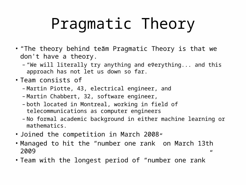
Pragmatic Theory• “The theory behind team Pragmatic Theory is that we don't have a

theory.” – “We will literally try anything and everything... and this approach has not let

us down so far.”• Team consists of

– Martin Piotte, 43, electrical engineer, and – Martin Chabbert, 32, software engineer, – both located in Montreal, working in field of telecommunications as

computer engineers– No formal academic background in either machine learning or mathematics.

• Joined the competition in March 2008• Managed to hit the “number one rank” on March 13th 2009• Team with the longest period of “number one rank”

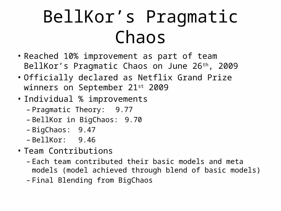
BellKor’s Pragmatic Chaos• Reached 10% improvement as part of team BellKor’s Pragmatic

Chaos on June 26th, 2009• Officially declared as Netflix Grand Prize winners on September 21st

2009• Individual % improvements

– Pragmatic Theory: 9.77– BellKor in BigChaos: 9.70– BigChaos: 9.47– BellKor: 9.46

• Team Contributions– Each team contributed their basic models and meta models (model

achieved through blend of basic models)– Final Blending from BigChaos

Dataset

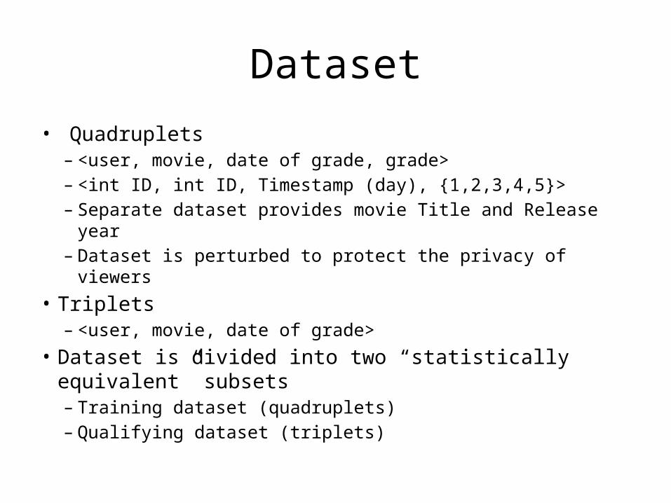
• Quadruplets– <user, movie, date of grade, grade>– <int ID, int ID, Timestamp (day), {1,2,3,4,5}>– Separate dataset provides movie Title and Release year– Dataset is perturbed to protect the privacy of viewers

• Triplets– <user, movie, date of grade>

• Dataset is divided into two “statistically equivalent” subsets– Training dataset (quadruplets)– Qualifying dataset (triplets)

Training Dataset(quadruplets)

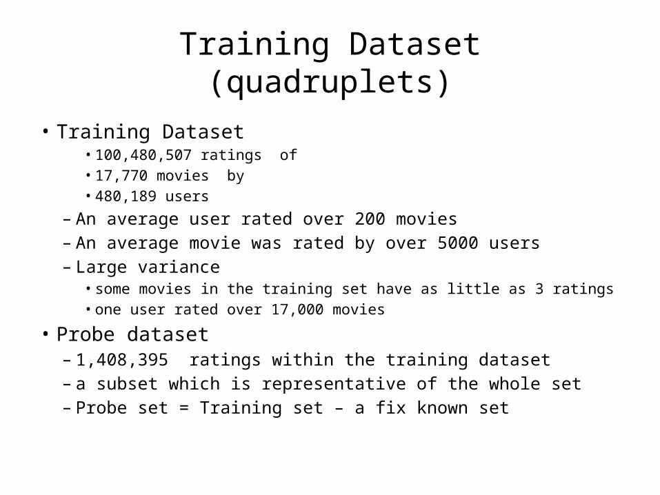
• Training Dataset• 100,480,507 ratings of • 17,770 movies by • 480,189 users

– An average user rated over 200 movies– An average movie was rated by over 5000 users– Large variance

• some movies in the training set have as little as 3 ratings• one user rated over 17,000 movies

• Probe dataset– 1,408,395 ratings within the training dataset– a subset which is representative of the whole set– Probe set = Training set – a fix known set

Qualifying Dataset(Triplets)

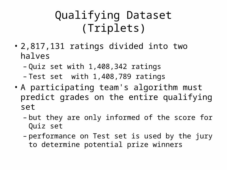
• 2,817,131 ratings divided into two halves– Quiz set with 1,408,342 ratings– Test set with 1,408,789 ratings

• A participating team's algorithm must predict grades on the entire qualifying set– but they are only informed of the score for Quiz

set– performance on Test set is used by the jury to

determine potential prize winners

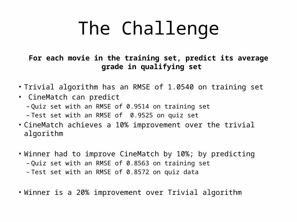
The ChallengeFor each movie in the training set, predict its average grade in qualifying set

• Trivial algorithm has an RMSE of 1.0540 on training set• CineMatch can predict

– Quiz set with an RMSE of 0.9514 on training set– Test set with an RMSE of 0.9525 on quiz set

• CineMatch achieves a 10% improvement over the trivial algorithm

• Winner had to improve CineMatch by 10%; by predicting– Quiz set with an RMSE of 0.8563 on training set– Test set with an RMSE of 0.8572 on quiz data

• Winner is a 20% improvement over Trivial algorithm

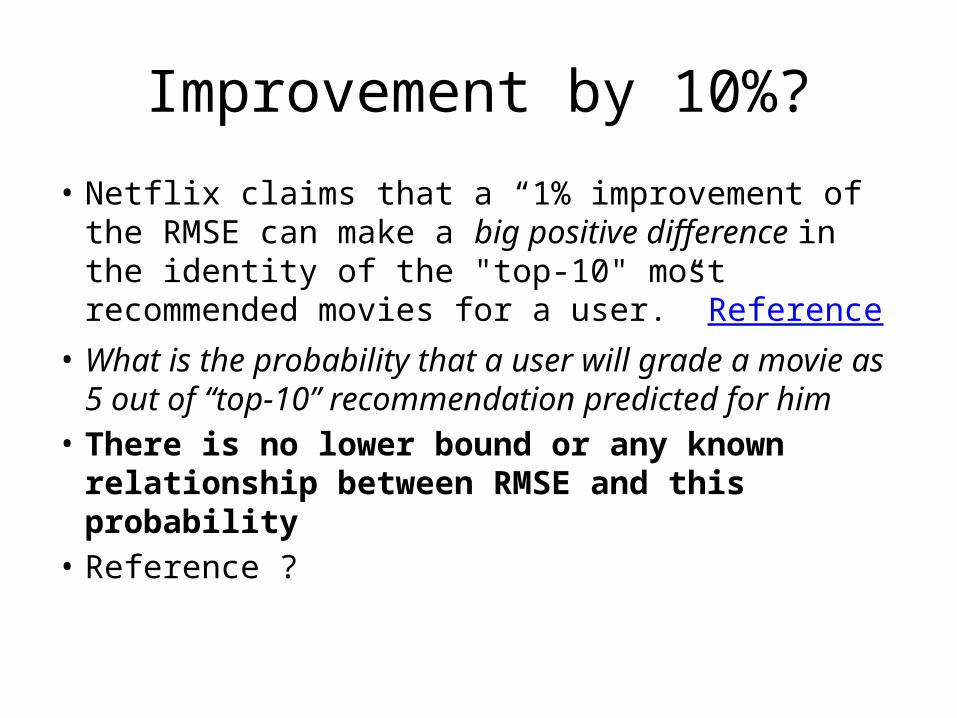
Improvement by 10%?

• Netflix claims that a “1% improvement of the RMSE can make a big positive difference in the identity of the "top-10" most recommended movies for a user.” Reference

• What is the probability that a user will grade a movie as 5 out of “top-10” recommendation predicted for him

• There is no lower bound or any known relationship between RMSE and this probability

• Reference ?

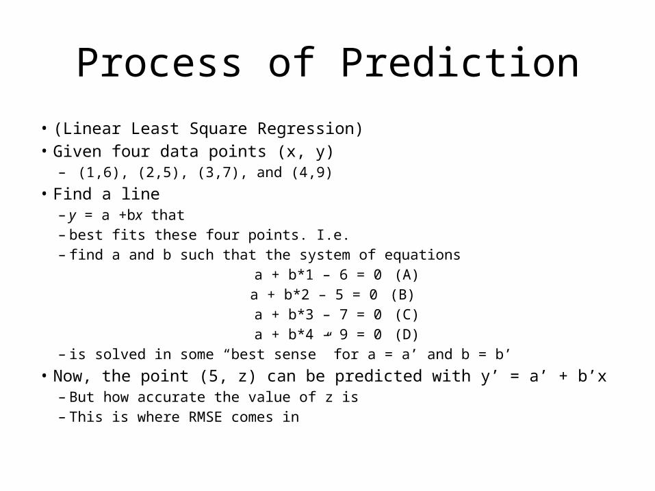
Process of Prediction• (Linear Least Square Regression)• Given four data points (x, y)

– (1,6), (2,5), (3,7), and (4,9)• Find a line

– y = a +bx that – best fits these four points. I.e. – find a and b such that the system of equations

a + b*1 – 6 = 0 (A)a + b*2 – 5 = 0 (B) a + b*3 – 7 = 0 (C)a + b*4 – 9 = 0 (D)

– is solved in some “best sense” for a = a’ and b = b’• Now, the point (5, z) can be predicted with y’ = a’ + b’x

– But how accurate the value of z is – This is where RMSE comes in

RMSE

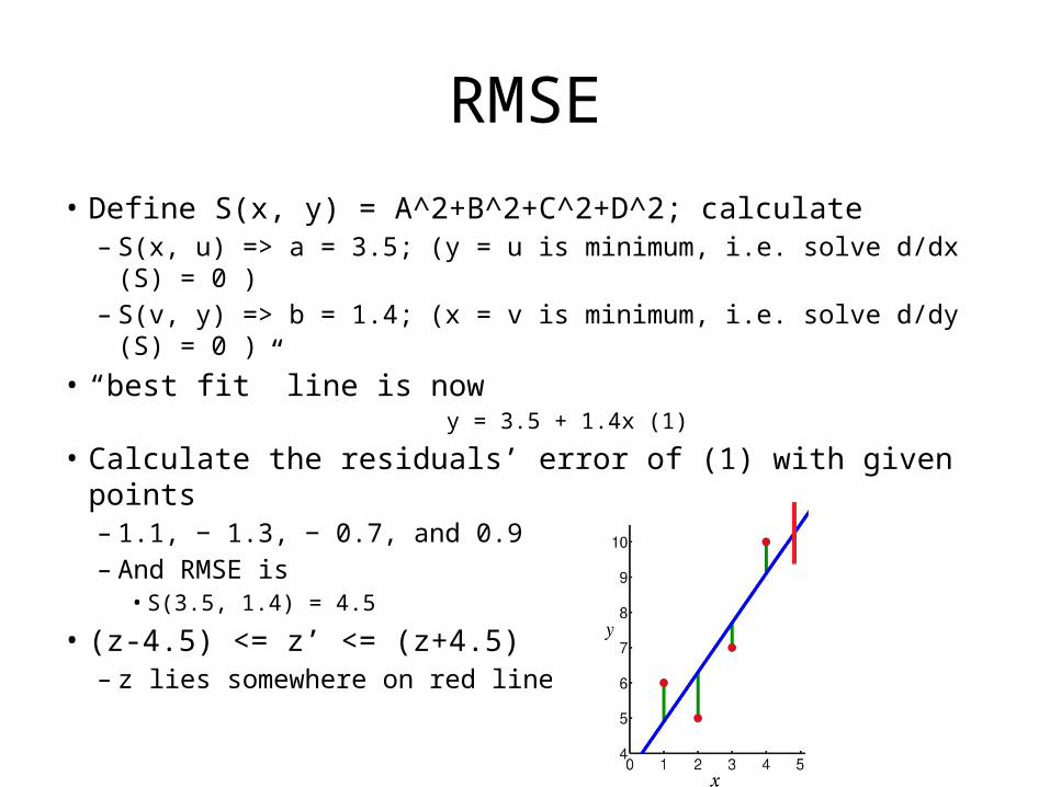
• Define S(x, y) = A^2+B^2+C^2+D^2; calculate – S(x, u) => a = 3.5; (y = u is minimum, i.e. solve d/dx (S) = 0 )– S(v, y) => b = 1.4; (x = v is minimum, i.e. solve d/dy (S) = 0 )

• “best fit” line is now y = 3.5 + 1.4x (1)

• Calculate the residuals’ error of (1) with given points– 1.1, − 1.3, − 0.7, and 0.9 – And RMSE is

• S(3.5, 1.4) = 4.5

• (z-4.5) <= z’ <= (z+4.5)– z lies somewhere on red line

Model and Meta-Parameters

• M1: the line y = 3.5 + 1.4x is a prediction model– a = 3.5 and b = 1.4 are meta-parameters or

predictors of this model– The model has a precision of 4.5

• M2: a second model can be generated by “best fitting”, say, y = ax^2+bx+c– a = a’, b = b’ and c=c’ with a precision of RMSE– M2 would be better then M1 if RMSE < 4.5

Blending or “Meta-Equations”• Now, what about be the RMSE of

– Y = foo*M1 + bar *M2, where (foo + bar) = 1– A linear combination of predictors

• Blending is the process of “approximating the approximators”– It is “best fitting” of approximation curves to represent original data– Its works on predictors, not on original data

• Recursive prediction– Level 0: given, the original data set – Level 1: a predictor, best fit of data set (RMSE-1)– Level 2: a blend, best fit of two or more predictors (RMSE-2 <= RMSE-1)– Level N: a blend, best fit of two or more predictors or blends or a combination

• (RMSE-N <= RMSE)– Winner

• A blend of two or more predictor is in itself a valid predictor• More on blending later

Pragmatic Theory contribution to

BPC

• Nearly 500 predictors• 44 different models with 577 unique variants

– BK4 with 128 variants– Matrix Factorizations 1 with 57 variants– 5 different models each contributing 2 variants only– 5 different models each contributing 1 variant only

• 906 Blends– 457 blends with Neural Nets– 444 blends without Neural Nets– 5 Quiz Set Variable Multiplication blends

Predictors: the Good, the Bad, and the Ugly

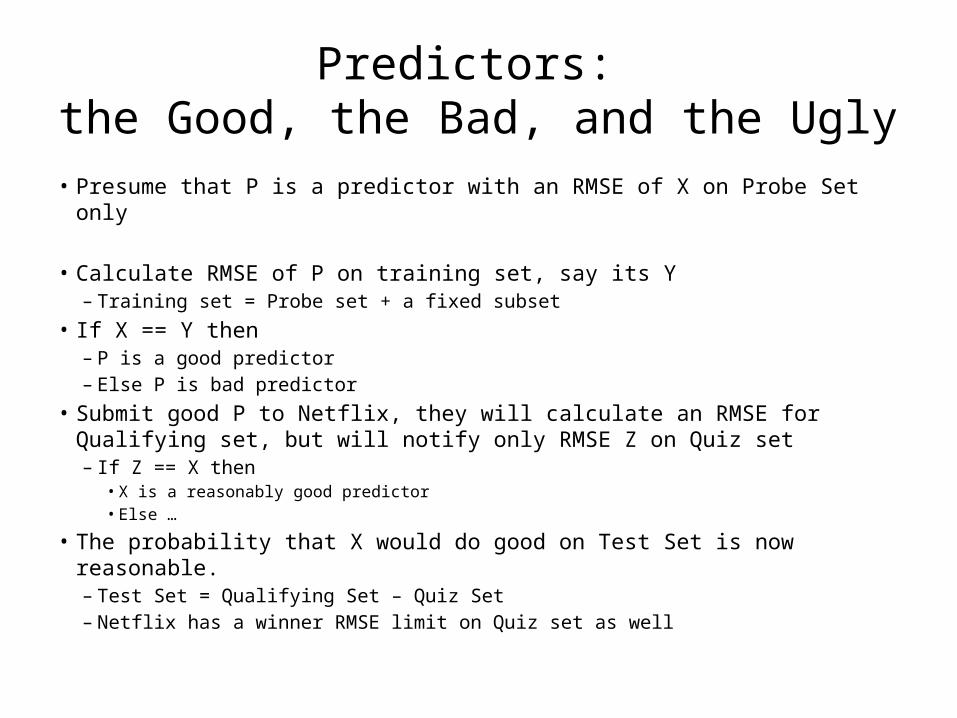
• Presume that P is a predictor with an RMSE of X on Probe Set only

• Calculate RMSE of P on training set, say its Y– Training set = Probe set + a fixed subset

• If X == Y then – P is a good predictor – Else P is bad predictor

• Submit good P to Netflix, they will calculate an RMSE for Qualifying set, but will notify only RMSE Z on Quiz set– If Z == X then

• X is a reasonably good predictor• Else …

• The probability that X would do good on Test Set is now reasonable.– Test Set = Qualifying Set – Quiz Set – Netflix has a winner RMSE limit on Quiz set as well

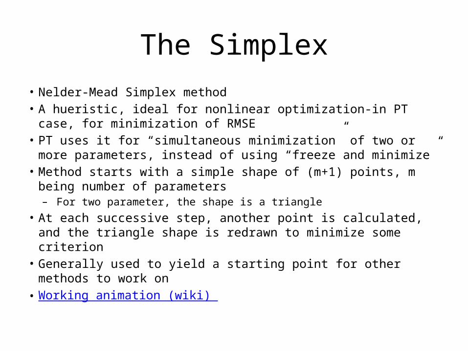
The Simplex• Nelder-Mead Simplex method• A hueristic, ideal for nonlinear optimization-in PT case, for

minimization of RMSE• PT uses it for “simultaneous minimization” of two or more

parameters, instead of using “freeze and minimize”• Method starts with a simple shape of (m+1) points, m being number

of parameters– For two parameter, the shape is a triangle

• At each successive step, another point is calculated, and the triangle shape is redrawn to minimize some criterion

• Generally used to yield a starting point for other methods to work on• Working animation (wiki)

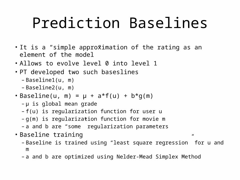
Prediction Baselines• It is a “simple approximation of the rating as an element of the model”• Allows to evolve level 0 into level 1• PT developed two such baseslines

– Baseline1(u, m)– Baseline2(u, m)

• Baseline(u, m) = µ + a*f(u) + b*g(m)– µ is global mean grade– f(u) is regularization function for user u– g(m) is regularization function for movie m– a and b are “some” regularization parameters

• Baseline training– Baseline is trained using “least square regression” for u and m– a and b are optimized using Nelder-Mead Simplex Method

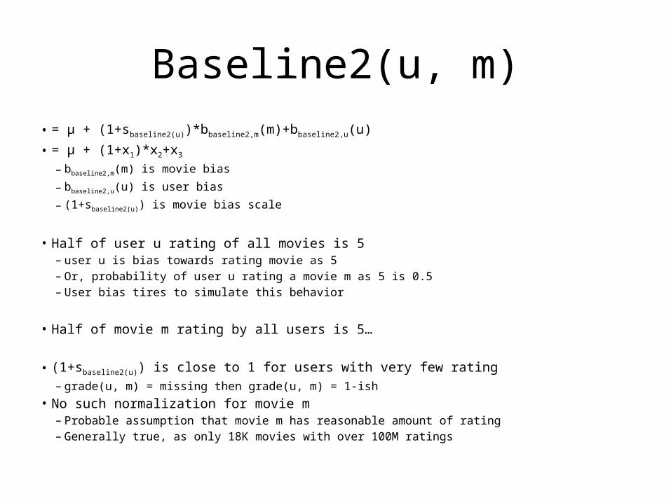
Baseline2(u, m)• = µ + (1+sbaseline2(u))*bbaseline2,m(m)+bbaseline2,u(u)

• = µ + (1+x1)*x2+x3

– bbaseline2,m(m) is movie bias

– bbaseline2,u(u) is user bias

– (1+sbaseline2(u)) is movie bias scale

• Half of user u rating of all movies is 5– user u is bias towards rating movie as 5– Or, probability of user u rating a movie m as 5 is 0.5– User bias tires to simulate this behavior

• Half of movie m rating by all users is 5…

• (1+sbaseline2(u)) is close to 1 for users with very few rating– grade(u, m) = missing then grade(u, m) = 1-ish

• No such normalization for movie m– Probable assumption that movie m has reasonable amount of rating– Generally true, as only 18K movies with over 100M ratings

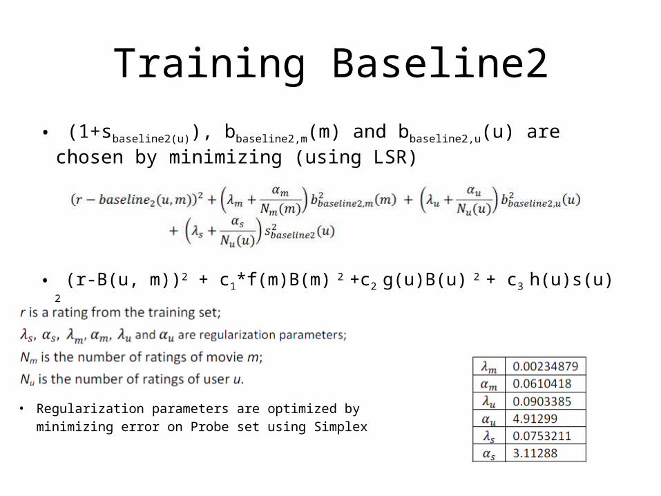
Training Baseline2• (1+sbaseline2(u)), bbaseline2,m(m) and bbaseline2,u(u) are chosen by minimizing

(using LSR)

• (r-B(u, m))2 + c1*f(m)B(m) 2 +c2 g(u)B(u) 2 + c3 h(u)s(u) 2

• Regularization parameters are optimized by minimizing error on Probe set using Simplex

The BK Models• BK for BellKor• 184 variants of 5 flavors of BK• Models are linear but with a non-linear envelope

– Linear model * nonlinear factor• It can even model behavior of two users who are sharing an account (family Netflix account)• Latent features: rating has a “time components”

– Frequency of “5” rating– Number of rating by user u in a day– Number of rating of movie m in a day – Avg. date of rating, relative to prediction– Rating based movie “grouping” – Movie Neighborhood prediction– Movie Appreciating vs. Movie rating

• User u “5” might not be the same as user v “5”

• Frequency based models are most used– 128 models out of total 184 BK models– Around 500 total

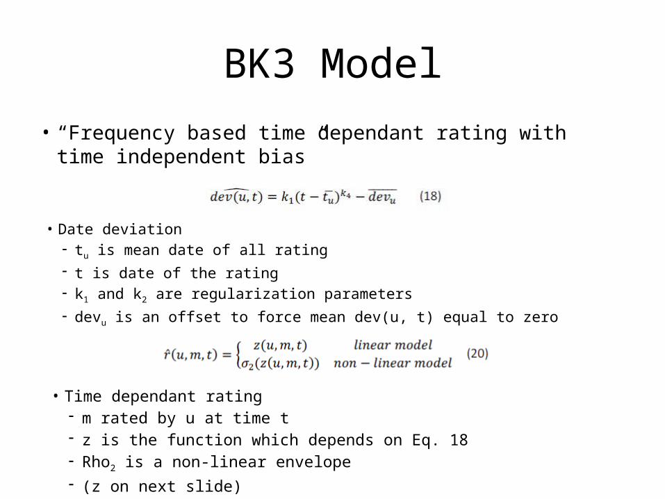
BK3 Model• “Frequency based time dependant rating with time independent

bias”

• Date deviation - tu is mean date of all rating- t is date of the rating- k1 and k2 are regularization parameters- devu is an offset to force mean dev(u, t) equal to zero

• Time dependant rating- m rated by u at time t- z is the function which depends on Eq. 18- Rho2 is a non-linear envelope- (z on next slide)

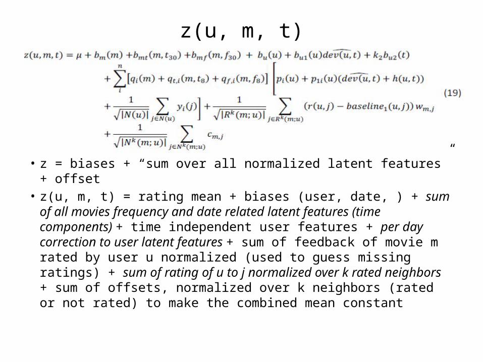
z(u, m, t)

• z = biases + “sum over all normalized latent features” + offset• z(u, m, t) = rating mean + biases (user, date, ) + sum of all movies

frequency and date related latent features (time components) + time independent user features + per day correction to user latent features + sum of feedback of movie m rated by user u normalized (used to guess missing ratings) + sum of rating of u to j normalized over k rated neighbors + sum of offsets, normalized over k neighbors (rated or not rated) to make the combined mean constant

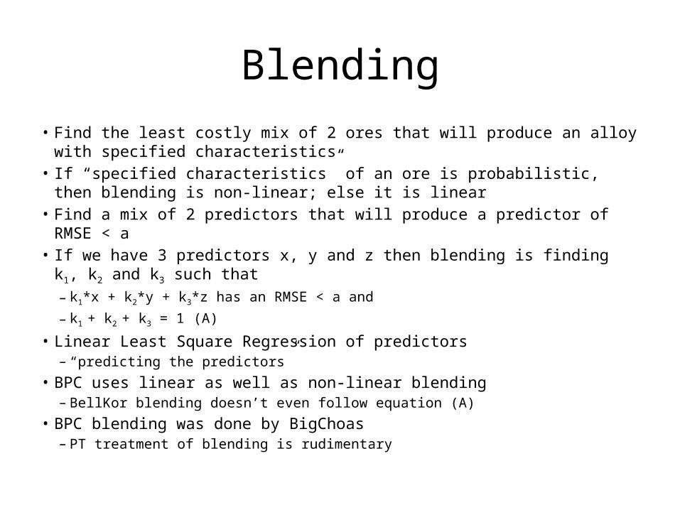
Blending• Find the least costly mix of 2 ores that will produce an alloy with specified

characteristics• If “specified characteristics” of an ore is probabilistic, then blending is non-

linear; else it is linear• Find a mix of 2 predictors that will produce a predictor of RMSE < a• If we have 3 predictors x, y and z then blending is finding k1, k2 and k3 such that

– k1*x + k2*y + k3*z has an RMSE < a and

– k1 + k2 + k3 = 1 (A)

• Linear Least Square Regression of predictors– “predicting the predictors”

• BPC uses linear as well as non-linear blending– BellKor blending doesn’t even follow equation (A)

• BPC blending was done by BigChoas– PT treatment of blending is rudimentary

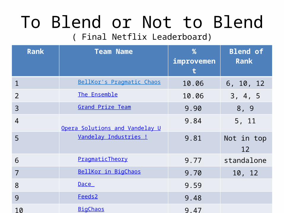
To Blend or Not to Blend( Final Netflix Leaderboard)

Rank Team Name % improvement

Blend of Rank

1      BellKor's Pragmatic Chaos 10.06 6, 10, 12

2      The Ensemble 10.06 3, 4, 5

3      Grand Prize Team 9.90 8, 9

4      Opera Solutions and Vandelay United 9.84 5, 11

5      Vandelay Industries ! 9.81 Not in top 12

6      PragmaticTheory 9.77 standalone

7      BellKor in BigChaos 9.70 10, 12

8      Dace_ 9.59

9      Feeds2 9.48

10      BigChaos 9.47

11      Opera Solutions 9.47

12      BellKor 9.46

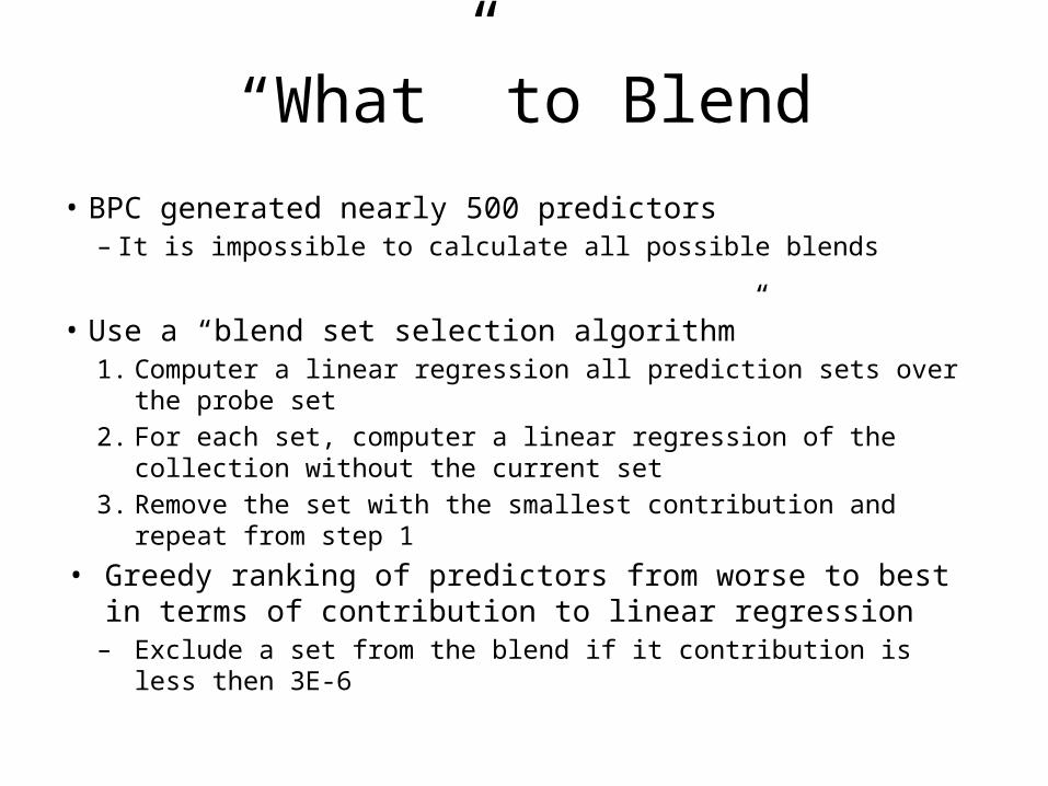
“What” to Blend

• BPC generated nearly 500 predictors– It is impossible to calculate all possible blends

• Use a “blend set selection algorithm”1. Computer a linear regression all prediction sets over the probe set2. For each set, computer a linear regression of the collection

without the current set3. Remove the set with the smallest contribution and repeat from

step 1• Greedy ranking of predictors from worse to best in terms of

contribution to linear regression– Exclude a set from the blend if it contribution is less then 3E-6

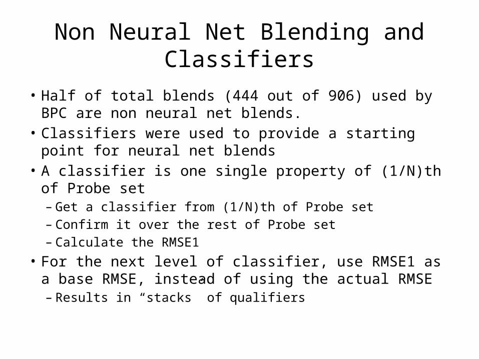
Non Neural Net Blending and Classifiers

• Half of total blends (444 out of 906) used by BPC are non neural net blends.

• Classifiers were used to provide a starting point for neural net blends

• A classifier is one single property of (1/N)th of Probe set– Get a classifier from (1/N)th of Probe set– Confirm it over the rest of Probe set– Calculate the RMSE1

• For the next level of classifier, use RMSE1 as a base RMSE, instead of using the actual RMSE– Results in “stacks” of qualifiers

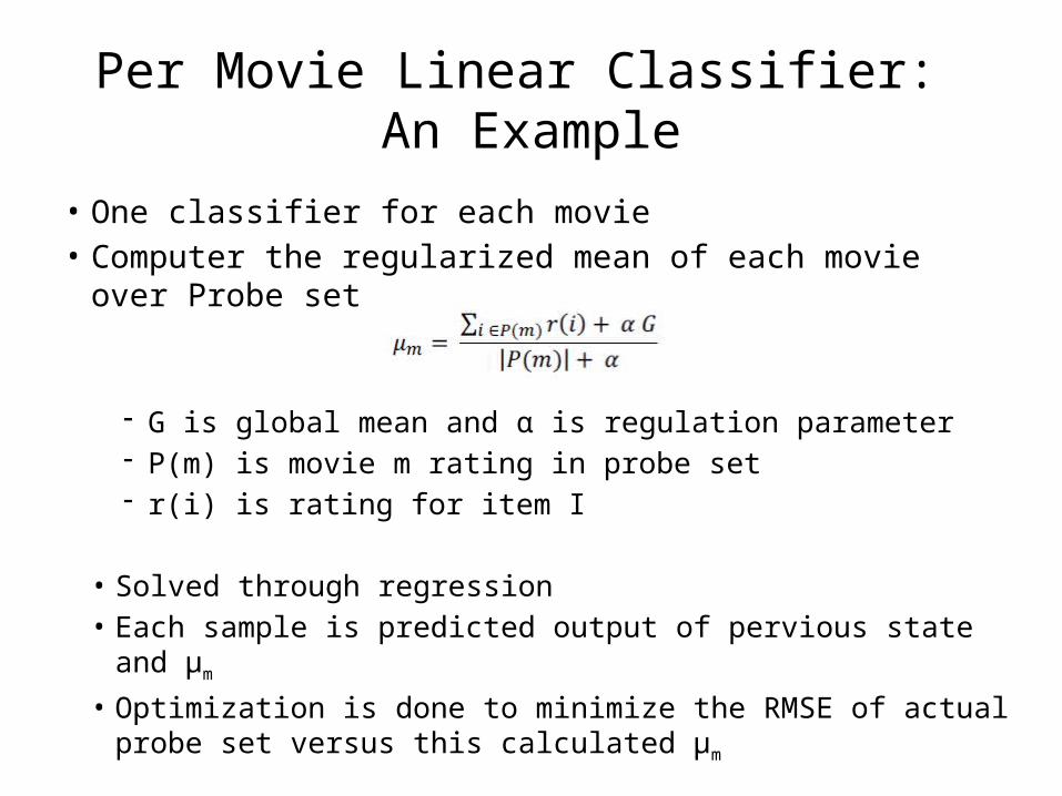
Per Movie Linear Classifier: An Example

• One classifier for each movie• Computer the regularized mean of each movie over Probe set

- G is global mean and α is regulation parameter- P(m) is movie m rating in probe set- r(i) is rating for item I

• Solved through regression• Each sample is predicted output of pervious state and µm • Optimization is done to minimize the RMSE of actual probe set

versus this calculated µm

Variable Multiplication Blend• Final step of BPC is a linear regression blend done directly on Quiz set

• In its simplest, multiple predictors are developed solely on quiz set and then they are multiplied together– Linear predictor * non-linear predictor = non-linear predictor

• Forward Selection– Construct a baseline on 233 sets of pragmatictheory blend using linear

regression– Add, multiple of each possible pair of predictor, and then blend again – Select the pair which improves the blend most– Add selected pair to baseline, and run the algo again– Repeat this N times

• 15 such predictors were chosen and included in the final blend

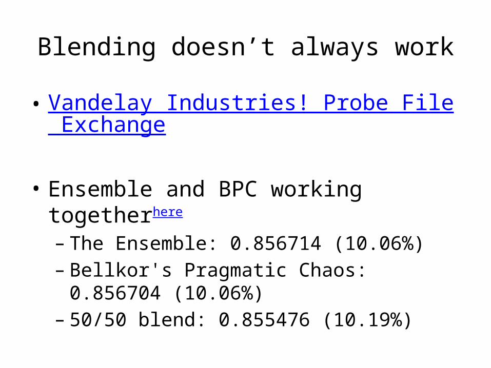
Blending doesn’t always work

• Vandelay Industries! Probe File Exchange

• Ensemble and BPC working togetherhere – The Ensemble: 0.856714 (10.06%)– Bellkor's Pragmatic Chaos: 0.856704 (10.06%) – 50/50 blend: 0.855476 (10.19%)

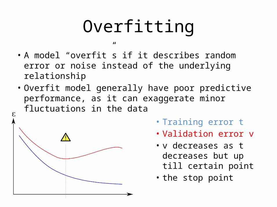
Overfitting

• A model “overfit”s if it describes random error or noise instead of the underlying relationship

• Overfit model generally have poor predictive performance, as it can exaggerate minor fluctuations in the data

• Training error t• Validation error v• v decreases as t

decreases but up till certain point

• the stop point

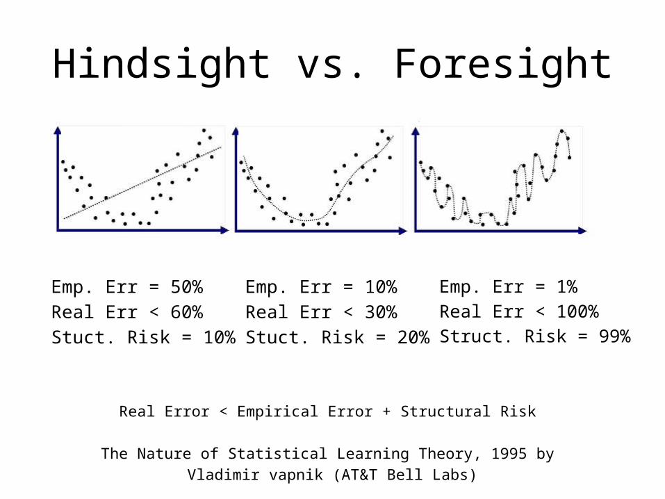
Hindsight vs. Foresight

Emp. Err = 50%Real Err < 60%Stuct. Risk = 10%

Emp. Err = 1%Real Err < 100%Struct. Risk = 99%

Emp. Err = 10%Real Err < 30%Stuct. Risk = 20%

Real Error < Empirical Error + Structural Risk

The Nature of Statistical Learning Theory, 1995 by Vladimir vapnik (AT&T Bell Labs)

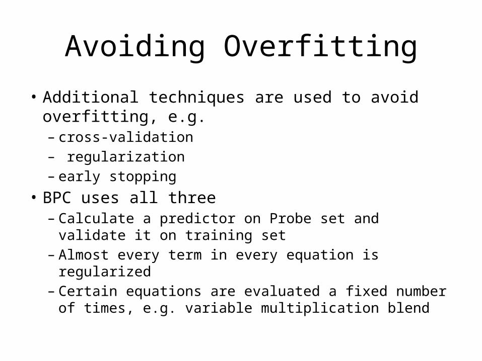
Avoiding Overfitting

• Additional techniques are used to avoid overfitting, e.g. – cross-validation– regularization – early stopping

• BPC uses all three– Calculate a predictor on Probe set and validate it on training

set– Almost every term in every equation is regularized– Certain equations are evaluated a fixed number of times,

e.g. variable multiplication blend

• Questions, Comments….

References

• Pragmatic Theory official page at this link• Wiki page on Netflix prize at this link• Wiki page on Linear Least Square at this link• Wiki page on Simplex at this link• Netflix Community entry on Blending, this link• Overfitting: when accuracy measures goes

wrong at this link