Embed Size (px)
Citation preview
bull
THE PREDICTION OF HYDRODYNAMIC VISCOUS DAPING OF OFFSHORE STRGCTURES IN WAVES AND CURRENT ay
THE STOCHASTIC LINEARIZATION METHOD
By
PRANAB KUMAR GHOSH
BTECH INDIAN INSTITUTE OF TECHNOLOGY KHARAGPUR INDIA (1976)
SUBMITTED IN PARTIAL FULFILLMENT OF THE REQUIREMENTS FOR THE DEGREE OF MASTER OF SCIENCE
At the
MASSACHUSETTS INSTITUTE OF TECHNOLOGY May 1983
) Massachusetts Institute of Technology 1983
fraVamptb c Glucpound Signature of Author Department of Ocean Engineering
_May 1983 bull
Certified by bullbullbullbullbullbullbullbullbullbullbullbullbullbull~bullbullbull1~ L-~-~~-~--- J Kim Vandiver
Thesis Supervisor
Accepted by bull bullbullbullbullbullbullbullbullbullbullbullbullbullbullbullbullbullbullbullbullbullbullbullbullbullbullbullbullbullbullbullbullbullbullbullbullbullbullbullbullbullbullbullbullbullbullbullbullbullbull ADouglas Carmichael
Departmental Graduate Committee
THE PREDICTION OF HYDRODYNAMIC VISCOUS DAMPING OF OFFSHORE STRUCTURES IN WAVES AND CURRENT
BY THE STOCHASTIC LINEARIZATION METHOD
By
PRANAB KUMAR GHOSH
Submitted to the Department of Ocean Engineering on May 6 1983 in Partial Fulfillment of
the Requirements for the Degree of Master of Science in Ocean Engineering
ABSTRACT
The hydrodynamic viscous damping and response statistics of certain kinds of offshore structures subjected to unidirectional wave-current excitation have been predicted By applying the technique of stochastic linearization the nonlinear equation for dynamic response is linearized and then approximate predictions are made for the damping and response Examination of the final derived relations reveals that both waves and current in addition to contributing to the excitation force cause additional damping Usefulness of the stochastic linearization technique has been demonstrated by analyzing a shallow water Caisson and a deep water guyed tower
In addition to the dynamic response the equation for the mean static response under the combined wave-current excitation has been derived It has been demonstrated that the mean static response depends on the seastate in addition to current
Thesis Supervisor J Kim Vandiver PhD
Title Associate Professor of Ocean Engineering
bull
3
ACKNOWLEDGEMENTS
I am indebted to Prof J Kim Vandiver His friendship
guidance and willingness to allow me to pursue my own ideas made
my research work enjoyable Funding for a portion of this work
was provided by the Minerals Management Service
4
TABLE OF CONTENTS
10 INTRODUCTION 5
11 General Remarks 5
12 Purpose and Scope of Present Work 5
20 NONLINEAR RANDOM VIBRATION 6
30 STOCHASTIC LINEARIZATION METHOD 7
40 DAMPING AND RESPONSE PREDICTION 11IN WAVES AND CURRENT
41 Formulation 11
411 Linearization 12
412 Solution 16
42 Computation 22
421 The Caisson with Low Response 24Amplitude
422 Flexible Caisson 28
423 Guyed Tower 30
50 SUMMARY AND CONCLUSIONS 34
6 bull 0 REFERENCES 36
Appendix A 38
Appendix B 39
Appendix C 42
Figures 44
ll General Remarks
Efforts to make more accurate prediction of response of
structures in random environment have resulted in increased
application of probabilistic methods The theory for prediction
of stationary response of linear structures to Gaussian
excitation is well developed However many structures
including offshore structures exhibit different forms of
nonlinearity When non-linearities are important the response
probability distributions are no longer Gaussian and in general
closed form solutions do not exist
Over the last two decades different approximate techniques
have been developed for solution of this problem However their
application to offshore structures is extremely limited
12 Purpose and Scope of the Present Study
In the present study a method of prediction of the
wave-current induced response of offshore structures is presented
using the Stochastic Linearization method Because of the
inclusion of ocean current the flow velocity is a nonzero-mean
Gaussian random process This causes the nonlinear hydrodynamic
force to be asymmetric It wil be shown that despite the
asymmetry the Stochastic Linearization method yields equations of
manageable complexity
Two structures of completely different dynamic
characteristics have been chosen as examples One is a stiff
shallow water sinale pile caisso1 and the otlier is cl compliant
i 1 ~- - l t -~- - i
b
and the response quantities are predicted in the presence of
waves and current A number of parametric studies have been
conducted to demonstrate the influence of different structural
parameters on the dynamic behaviour
The main focus of this study is on the prediction of
response and viscous hydrodynamic damping in moderate sea states
20 NONLINEAR RANDOM VIBRATION
Strictly speaking linearity in structures is never
completely realized Nonlinearities are present in stiffness
damping mass or in any combination of these However for
offshore structures a primary source of nonlinearity is the
nonlinear hydrodynamic force
There are several approximate methods for dealing with
nonlinear random vibration problems The particular problem of
an oscillator with nonlinear stiffness and excited by white noise
is the only problem that has been solved exactly The method of
solution is commonly known as the Markov Vector method
(Lin1968) The differential equation for the joint probability
density of response displacement and velocity called the
Fokker-Planck equation has been set up and solved exactly
However for nonlinear damping the Fokker-Planck equation can be
solved numerically only Recently this method has been applied
to offshorP structures (Rajagopalon 1982 Brouwers1982)
In the perturbation method the solution is expanded in a
power series First developed by Crandall (Crandall1963) this
S~Strlt1S
7
Generally the solution is approximated by the first few te~ms of
the series only The higher order terms particularly for
nonwhite excitation is very laborious to obtain The response
is approximated as a Gaussian process Offshore steel jacket
platforms have been analysed by this method (Taylor 1982)
The functional power series expansion suggested by Volterra
(Volterra 1930) has been used by Weiner (Weiner 1958) for the
nonlinear stochastic process
In the Gaussian Closure technique relations between second
and higher order moment statistics are derived from the equation
of motion The higher order moments are decomposed into the
lower order moments using special Gaussian properties Finally
application of Fourier Transformation yields relations between
cross and auto spectra involving the response and excitation
quantities This technique was proposed by Iyenger (Iyenger
1975) and later applied to offshore structures by Dunwoody
(Dunwoody 1980)
30 STOCHASTIC LINEARIZATION METHOD
Introduced by Booton (Booton 1954) this technique has been
generalised by Foster (Foster 1968) and later by Iwan and Yang
(Iwan 1972) This method can handle nonlinearities in stiffness
as well as damping The reason for choosing for this particular
method over others is that it is eas~2r to use Also the
reliability of this method is already proven
8
The main steF3 i~ AE~Dlication of tl1is tech~ique arc as
follows
(1) Replace nonlinear terms with equivalent linear terms
(2) Find the error which is the difference between the approximate linear and tte nonlinear terms
(3) Take the square of error and evaluate its expected value or first moment
(4) Minimize the mean square error by taking its derivative with respect to the equivalent linear coefficients
(5) Equate these derivatives to zero to obtain the relations between linear coefficients and known problem parameters
Consider the general equation of motion of a dynamic system
x + g(xx) = f (t) ( 3 l)
where g(xx) is a nonlinear function of x and x but with the
limitation that it is single valued and not an even function
Assume that an approximate solution is obtained from the linear
equation
( 3 2)
The error introduced by linearization is
pound = g(x~) - S x e - k x e ( 3 3)
Where is a random variable
The error is minimized by requiring the mean square error to
be minimum which implies
( 3 4) c e
a 2 -- - lts gt = O (3 5) ae
Substituting Eg (33) into Eqs (34) and (35) and
interchanging the order of differentiation and expectation we
obtain fron Eq (3 4)
lt_ [g(x~) - Bx - k x] 2 gt = Oas e e e
ie
B x bull2
ltg(x~)~ k xxgt = 0 ( 3 6)e e
Similarly from Eg (35)
ltg(x~)x - S xx - k x 2gt = O ( 3 7)
e e
Since the joint expectation of a random variable and its
derivative is zero Eqs (36) and (37) lead to
= ltg (x ~) ~gt6 ( 3 8) e ltxbull 2 gt
( 3 bull 9 jk e
If we further restrict ourselves to the case where the stiffness
and damping nonlinearities are separable then we can write
g (xxgt = f ltxJ + f ltxgt (310)1 2
where f (x) and f (x)
are nonlinear functions of x and x 1 2
respectively
Substitution of Eq (310) in Eqs (38) and (39) results
in
ltxt 2 ltxlgt (311)bull 2
ltx gt
(312)
From Eqs (311) and (312) we observe that the equivalent
linear coefficients are obtained by equating the input-output
cross correlations of the nonlinearities (eg xf (x)) and their2 linear approximations (eg xBex)
l L
40 c
41 For~ulation
Using a beam raode~ the flexural ibr~tion equation of an
offshore structure (eg Caisson Jacket or Guyed Tower) can be
written as
4 m (x) + EI~ + C aY + f(xt) ( 4 1)
s 4 satax
Where ms ( x) = Steel massunit length
EI = Flexural rigidity
c = Structural damping coefficient s
M = Deck mass
f(xt) is the loading due to waves and current which according
to Morison Formula is given by
( 4 bull 2 )
Where V ( XJ = Volume of structureunit length CM = Added mass coefficient p = Mass density of water u (xt) = Wave induced horizontal water particle
velocity V (x) = Current speed D = Total projected area perpendicular to
the flow The formulation is based on the assumption that the Morison
Formula can be applied to express drag in terms of the relative
fluid-structure velocity
12
The first two terms of t(xt) stand for the inertia force
and the third term stands for the drag force
The hydrodynamic load model may not be very accurate for
multiple leg offshore structures like a Jacket or a Guyed Tower
This is because the spatial effect on the phase of wave forces on
legs and the loading on secondary cross members are neglected
Although the structural idealisation is crude its
consequences are not serious The simple beam model idealisation
adopted here is not used for solving the Eigenvalue problem In
the context of the present work the Eigenvalue solution is
assumed to be known The structural model adopted here is
satisfactory for investigation of the nonlinear effects of
seastate and current on dynamic response behaviour and viscous
hydrodynamic damping
411 Linearization
The presence of current causes asymmetric drag force Since
the drag force is a random process with a non-zero mean the
stationary solution of Eq (41) can be written in the following
form as a superposition
y(xt) = y0
(x) -L j(xt) (43)
where y0
(x) = Mean deterministic offset
y(xt)= Time dependent response
substituting Eqs (42) and (43) into Eq (41) we obtain
2v 4 m ~+EI~+
satL ax4
a4yEI~+
ax~
C f_ sat
2 + M_lt_Y_2at
o(x-1)
bull bull 1 bull I middotI= C~cVu - (C~-l)pVy + ~ocDD(u+V-y) u+V-yi
J __)
This equation can be recast in the following form
4 2 m + EI4 + c zx + MLY_ o(x-1) (CM-l)pVy + c (r)
s sat 2ax at ( 4 4)
Where
( 4 5)g(r) = pc0 o(r+V) jr+vl shy
g(r) is a nonlinear function of r which is the fluid-structure
relative velocity defined as
r = u - y (4 6)
In the stochastic linearization approach g(r) is replaced
by Cer where Ce is the equivalent linear coefficient The
meansquare error between the nonlinear term and its linear
approximation is given by
lt[g(r) - Cer] 2 gt = E ( 4 7)
The equivalent linear coefficient is obtained by equating
the derivative to zero
lt [g(r) - Cer] 2 gt ( 4 8)
Interchanging the order of differentiation and expectation
leads to
lt2[g(r) - C r]rgt = 0 e
= ltCJ(r)rgt ( 4 9)Ce 2 ltr
The quantity ltg(r)rgt is very difficult to evaluate beshy
cause g(r) is related to r in a very complex manner However
the quantity on the right hand side of Eq (49) satisfies
the following Gaussian identity
ltg(r)rgt = ltddr g(r)gt (410)ltr2gt
Proof of this identity is in Appendix A
It turns out that for g(r) as defined in Eq (45) the
right hand side quantity of Eq (410) is far simpler to evaluate
than the left hand side quantity
The equivalent linear coefficient is
Ce= lt~r g(r)gt ( 4 ll)
The equivalent linear coefficient as defined by Eq (411)
is the expected value of the gradient of the nonlinear function
g ( r) bull
Substituting Eq (45) into Eq (411) and carrying out the
differentiation we get
( 4 12)
(r+V) is a non zero mean Gaussian random variable The
quantity lr+vl is evaluated in Appendix B
15
Using the result of Appendix B
v2 Ce = pc D [ ~ or exp(---2 ) + 2VErf (-v__ J (413)
2 D Yi 2or Lor
Where Erf(X) is the Error Function defined as
x Erf(x) = 2 f exp(-t 2 )dt
It is also known as the Probability Integral
or is the rms fluid-structure relative velocity
Spanos investigated the case of a single degree-of-freedom
system under wave-current loading and arrived at similar
expression for the equivalent damping coefficient (Spanos 1981)
Replacing the nonlinear term g(r) with the equivalent linear
term Eq (44) can recast in the following form
4 2()2 [m +(CM-l)p9]~ + EI4 + (C +C ) aYt + MY a(x-L)
s ()t ix s e 0 ()t (414)
From Eqs (413)and (414) we observe that waves and current
influence excitation on the structure as well as damping of the
structure
A component of damping is a function of sea state and
current Similarly there is a sea state and current dependent
exciting force
4 1 2 Solution
The structure response is expressed in terms of its normal
modes centi and generalised coordinates qi
N
y(xtl = I cent(x)q(t) (415)]_ ]_
i=l
For the ith mode the uncoupled modal equation is
Mq + Cq
+ Kq = N ( 4 16) ]_ ]_ ]_ ]_ ]_ ]_ ]_
Where Mi = Modal mass =
L 2 d 2 2f Tl (x)centdx+(C1-l)pf 17ltgtdx + Mcento(x-L0 s ]_ 0 ]_ ]_
ii = Modal stiffness =
2wM ]_ ]_
c ]_
= Modal damping =
+ ~pC fd 2DV Erf(VLcrr)cent~dx2 D i
0
~ = Modal non viscous damping ratio51
d = Depth of water
L = Length of structure
c ]_
(418)=~- = tsimiddot + Evimiddot2Mw ]_ ]_
Where E = Modal viscous damping ratiovi
CD 2 2 2exc(-V 2cr )artax= ]_4Mc ]_ ]_
(4 19)
v Erf (--) o dx]
for i
The modal wave-current induced exciting force is given by
d N 17ZQdx + U [~ f D exp(-V2
2ar2 )crrcentiz~x
]_ ]_ 0 1T ()
(420)d
+ f 2DV Erf (V2crr)Zcentdx]]_
0
In Eq (4 20) the following relations have been used for the
wave induced water particle velocity and acceleration at any
arbitrary depth
(421)
u = u z
0
18
Where u = Wave induced watar particle velocity on the 0
free surface
= Wave induced water particle acceleration on the
free surface
Cosh(kx)z = Depth attenuation factor = Sinh (kd)
k is the wave number
In terms of the modal quantities the variance of the
structural response is
2 cpq) gt
l l (422)
For Caisson or Jacket type offshore structures the natural
frequencies are widely separated and the damping is light
Because of this the responses in different modes can be
considered to be stochastically uncorrelated With this widely
used established hypothesis in structural dynamics the cross
terms on the right hand side of Eq (422) vanish and it
simplifies to
N N2 2 2 2 2 crs = lt I ltP q gt = I ltP crq (423)
l l l li=l i=l
Where cr = rms modal response in the i th modeqi
crs = rms response of structure
1 9
A simple expression for the v3rLance of the relative
fluid-structure velocity can be derived if the cross correlation
between the fluid particle velocity and the structural velocity
is neglected
Nbull 2 2 bull2 bull 2 lt (u-y) gt = ltU gt + lty gt = ltjlJ) gtlt
i=lI l l
In the above expression the cross correlation term has been
neglected
Substituting Eq (423) in this equation leads to
N 2 2 2I ltjloqw (424)l l li=l
wi is the natural frequency corresponding to ith mode
Eqs (419) (420) and (424) indicate that the damping and
excitation in any particular mode depend on the seastate and
responses in all modes This is a manifestation of the nonlinear
drag force
The response spectra of an offshore structure has two types
of peaks One corresponds to the quasi-static response of the
structure and is located at the wave spectral peak frequency
The other type is due to the resonant dynamic response of the
structure at its natural frequencies In this study we are
primarily concerned about low to moderate sea states and hEnce
the quasi-static response is negligible Therefore the response
variance can be computed considering the dynamic response peak
modal response varianc can be estimated by the half power
bandwidth method as follows
i 25Si (CJ) Iw=w
(J 2
l (425)= qi 2 32M1w1s1
Where S ( w) = Spectral density function of modal excitingl force corresponding to i th mode
A compact expression for the modal exciting force can be
written using the two auxiliary variables C and C a u
N = C u + C u (426)i a o a o
Since the fluid particle velocity and acceleration are
stochastically uncorrelated the spectral density function of
modal exciting force is
sl (w) = c 2 s~ (w) + c 2 s (w) (427) a o u uo
Where Su (w) = sdf of fluid particle velocity0
2= CJ S (w)11
suolwJ = sdf of fluid particle acceleration 4
=~s(w) l
S (w) is the sdf of wave elevation 11
Substituting in Eq (427) yields
(428)
Where pCD g d 2 2 c = - -[-- f Dexp (-V 2or ) orcent i Zdx
u 20
d + f 2DV Erf (V2or) cent Zdx]
1 0
21
The mean response of the structure can be determined by
requiring that the solution given by Eq (43) satisfies Eq
(44) on the average
This requirement leads to the following equation
ltg(rgt = 0
(429)
The expected value of the quantity on the right hand side of
Eq (429) has been derived in Appendix C
Substituting the result of Appendix C in Eq (429) leads to
a4y 0 1 2 2 rEI-- = 2pC0D[(V +or )Erf(Vv2or4ax
(430)
+~or exp(-V22or2 ]
This equation is the well known beam equation and the right
hand side quantity is the mean time independent wave-current
induced load It is interesting to note that the mean load is a
function of the sea state in additi0n to current The dependence
on the sea state is caused by the nonlinearity in drag force If
the drag force was linear the mean load would have been a
fun~tion of current 0nly
integration of Eq (4 30) and application of appropriate boundary
conditions
42 Computation
It is apparent from Eqs (419) and (420) that the modal
viscous damping and exciting force depend on the structural
response This necessitates the adoption of an iterative
procedure for the determination of the damping and response
From the computation done in this study it has been observed
that the rate of convergence depends primarily on the response of
the structure When the structural response is small in
comparison to fluid particle motion the rate of convergence is
rapid
The modal quantities given by Eqs (419) and (420) are
evaluated by numerical integration because most of the
quantities in the integrands are not defined analytically For
numerical integration Simpson three point rule is used In the
software developed five equally spaced integration stations are
used over the length of the structure The numerical integration
has the advantage that any arbitrary current profile and mode
shape can be handled These quantities need to be defined
numerically at the discrete integration stations
The d~mping and response prediction is made using the two
parameter Bretschneider wave spectrum defined as 4 4 w w
SLil = 3125 n o~ middotmiddotI --
Where ls = Significant wave height (ft)
w = W2ve frequency correspondina to p spectral peak (radsec)
The peak frequen~y (WP) if not known is estimated in the
following way For Bretschneider spectra the peak frequency is
evaluated using the following relation between the peak frequency
and the average zero crossing period(Tz) (Sarpkaya 1981)
The relation between the significant wave height (Hs) and
the average zero crossing period is proba)ilistic in nature
However for simplicity the following deterministic relation
proposed by Weigel (Weigel 1978) has been used
Tz = 1 723H middot 56 s (432)
Tz is in sec and Hs is in ft
The Error Function in Egs (419) and (420) is approximated
by the following (Abramowitz and Stegun 1965)
Erf(x) = 1 -1 (433)
middotwhere al = 278393
a2 = 230389
a3 = 000972
a4 = 078108
Some other approximations were tried But this particular
one has been found to be well behaved and works better than some
Error Function ie bet~een zero and one
A closed form expression can be derived for the modal
viscous damping when the structural response is negligible
compared to water particle motion This is done for the first
mode of a caisson in this section
Since the structural motion is negligible Eq (424)
becomes
= (J z (434)uo
Where Z is the Depth Attenuation Factor It is assumed that
current V obeys the same Depth Attenuation law This assumption
makes the derivation considerably simpler The choice of current
distribution profile is not crucial Since it has been shown in
the later part of this work that current distribution has
negligible influence on the damping and dynamic response
Based on the assumption made the current speed at any depth
can be expressed as
v = v z 0
Where V0
= Current speed at free surface
Substituting Eqs (434) and (435) in Eq (419) yields
2 2 2[~rd exp(-V 2cr )cr z~dxiVi = 0 uo uo l 0
d + f 2V Z Erf (V 12a ) cjl~dx
0 0 uo l 0
(436)
= Erf (V 2a ) ] 0 uo
(~
x J ZQ~dxl
0
The first mode of a caisson can be approximated by the
following trigonometric function
(437)
Substituting this approximation for the mode shape the
integration in Eq (436) can be evaluated as follows
Calling this integration G(centj we can write
d G ( cent) = f
0
l - i x - exp(---i) - Exp(- -c~) Jdx
2 J L
Performing termwise integration leads to
G(cent)
L2c
kd kdSi nee kdmiddot gt 1 e -1 = e
11d Tid)G (qi) ( 2 k Lcos-L + 2 TI sinr
(4 38)
Further simplification can be achieved when the depth of
water is nearly equal to caisson length ie d=l
Under this condition
3G ( ltjl) = 2k
(439)
The rms fluid particle velocity
H s (440)4
It can be expressed as a function of significant wave height only
by substituting Eq (432) in Eq (440)
Then Eq(440) becomes
2TI HS 4491 H middot (441)0 uo = middot 56 s1723 H x 4 = s
Furthermore
v 78Vc 0 = 44 (442)
H2cruo s
and 2 2v 61V
0 = 0 (443)2 88H2ouo s
For the wave number (K) using the deep water dispersion
relation and Eq (432) leads to
k = 2
w g
= (~)Tz
2 1 g
= g x
4 TI 2
(1 723H s
56 ) 2 = 412 112
HS (444)
Substituting Eqs (441) (442) and (443) in Eq (436)
yields
261V 78V (16 x 91 H ~ 4 exp(- 0
) + 2V Erf( 4 ~)]G(cent)s H bull 88 o H bull s s
= 261V bull 78V
[l 456H ~ exs(----0 ) + 2V Erf( bull 4 ~]s(rJi)s middot H 88 0 11 s s (4 45)
G(cent) which is a function of the mode shape is given by either
Eq (438) or Eq (439)
The wave number (k) which is needed in the evaluation of
G ( q) is given by Eq ( 4 4 4)
Eq (445) provides a means for the prediction of modal
viscous da~~ing of a c2isson in pregtence of waves and current
This equation is not very accurate for the prediction purposes
but it gives a feel for relative influences of different
28
422Fle~ibl~ Ca~son
The Caisson analyzed in this section is located at West
Cameron Block 32 in the Gulf of Mexico It is owned and operated
by Mobil Oil Co The particulars of the Caisson are as below
Total Length = 2300 ft Water Depth = 1750 ft Leg Diameter = Tapers From 16 ft at Mudline to
8 ft at the Waterline Steel Mass = Varies From 18142 slugsft at
Mudline to 2465 slugsft at deck level
Deck Mass = 248450 slugs Natural Frequency = 289 radsec Non viscous Damping = 14 The Caisson is assumed to respond in the first mode only and
the mode shape is shown in Fig2
A sensitivity analysis has been carried out and the
influence of the following engineering parameters on the dynamic
behaviour of the Caisson has been studied
(1) Sea state defined by significant wave height(Hs)
(2) Current speed (V)
(3) Frequency ratio defined as the ratio of the first natural frequency of the structure (wn) and the peak spectral frequency(wp)
(4) Drag coefficient(CD)
(5) Current distribution parameter (Cvgtmiddot This is defined as the ratio of the area under the current distribution profile and the area of the largest rectangle enclosing it A linear profile has a ratio of 12
Figs 4 and 5 show the variatiun of damping and response
with sea state and current speed Damping increases considerably
with current speed and significant wave height The response
increases with sea state (Fig 5) but is hardly i~fluenced by
cmiddoturri~nt
contribute to both e~~itation ar1J d~mping~ T~ercfore the
variation of response ~ith changing sea state or current depends
on the relative magnitudes of modifications in damping and
excitation For the Caisson the response increases with sea
state because the increase in excitation is not fully offset by
the increase in damping Similarly the response increases with
current b8cause the i~=rease in 9xcitati0~ is not fully offset
by the increase in damping due to current
The deck response standard deviation and the modal damping
ratio are plotted agai~st the frequency ratio (wnwp) in Figs 6
and 7 Damping is found to be inversly related to frequency
ratio The plot of response standard deviation vs frequency
ratio resembles the response behaviour of a deterministic dynamic
system under harmonic excitation Like the resonance of a
deterministic system the response standard Jeviation reaches its
peak when the frequency ratio is close to one
In the present analysis a constant drag coefficient has been
used However the drag coefficient is a function of Reynold No
and Keulegan Carpenter No This means that the drag coefficient
is time dependent and also varies along the length of the
structure To find out the consequences of applying a constant
drag coefficient da~ping and response standard deviation have
been plotted against the drag coefficient (C ) in Figs 8 9 100
and 11 The response is found to be rather insensitive to drag
coefficient The damping increases with the drag coefficient
30
distribution i13~e ne0ligi~le effects on darriping and response
423 Guved Tower
In this section the results of an analysis for a Guyed
Tower are presented The purpose here is not to predict the
design values but to present characteristic response quantities
The relative significance of some important environmental and
structural parameters is investigated and some specific
conclusions drawn
A Guyed Tower is a compliant structure (Fig 13) The guy
lines provide the soft restoring force The tower is essentially
a truss work built between four corner legs The tower rests on
a piled foundation The tower base can be idealised to be free
to rotatebut fixed against sliding
The particulars of the specific tower considered are
given below
Total Length = 18040 ft
Water Depth = 16892 ft
Leg Diameter = 656 ft
Steel Mass = 5300 slugsft
Deck Mass = 3742940 slugs
Sway Mode Natural Frequency = 20 radsec
Bending Mode Natural Frequency = 14 radsec
Bending Mode Non Viscous Damping = 20
The first two natural modes of vibration are shown in Fig
14 In the present analysis it is assumed that the tower
~- --middot -middot middot middot-middot
middot J
rotation and the response i1 this mode is determined by the tower
mass and guy stiffness This is referred to as the sway mode
The response in the second mode called the bending mode here is
dictated by the tower mass and flexural stiffness
The response in the sway mode is not computed here This
mode is primarily excited by the second order wave forces and
wind forces both of which are difficult to model in the
frequency domain in spectral terms The standard deviation of
the sway mode response is input as a known quantity
The two quantities that have been predicted are the viscous
damping ratio and the standard deviation of deck response in the
bending mode The second response quantity is by itself not very
important because the deck response is primarily caused by the
sway mode However the deck response in the bending mode is a
measure of the tower bending moment Because the standard
deviation of bending moment is directly proportional to the
standard deviation of displacement response
The influence of the following parameters on the bending
mode response has been investigated
(1) Significant wave height (Hs)
(2) Current speed (V)
(3) Standard deviation of dee~ response in the sway mode ( J s )
37
(4) Ratio of benJinJ soJe natural frequency and frequency (_ middotmiddot- middot)of somiddot~-cl - - l- - -~ bullmiddotmiddotmiddot rt ~ p
(5) Current distribution parameter (Cy) which has already been defined
(6) Drag coefficient (C0 )
The sway mode motion influences the damping and excitation in the
bending mode through Eq (424)
Examination of Figs 15 16 17 18 19 20 reveals that the
damping in the bending mode is very sensitive to current and the
sway mode response but very little influenced by the sea state
This is because wave induced water particle velocity attenuates
v-dry rapidly in moderate sea states It is predominant near the
free surface Therefore the standard deviation of relative
fluid-structure velocity (Or) and the equivalent damping
coefficient are dominated by the sway mode response and ocean
current The response in the bending mode increases initially
with significant wave height (Figs 16 18 20) but then flattens
out for high sea states This is probably because the spectral
peak frequency moves away from the bending mode natural frequency
as the significant wave height goes up
Although the standard deviation of bending mode response
decreases with increasing current (Fig 16) the
rms response will not necessarily follow the same trend
Because the rms value depends on mean deflection which
increases with current (Eq 430)
In Figs 22 and 24 the bending mode response standard
deviation has been plotted against the frequency ratio The
resonance like effect is noticeable here also li~e tl1e Caisson
From Fig 25 it is observed that damping increases and
response decreases as the variation of current with depth gets
more uniform
In Fig 26 damping and response are plotted against drag
coefficients Unlike the caisson damping increases and response
decreases with increasing drag coefficients
)
50 c)1 -middotmiddotmiddot --middot- -middot ___middot~
A simple approach based on the Stochastic Linearization
technique has been presented for the dynamic response analysis of
offshore structures excited by waves and current Because of
the presence of current the drag force is asymmetric
Consequently the stationary solution for structural response
consists of superposition of a time independent deterministic
offset and a randomly fluctuating component The main focus in
this study has been on the randomly fluctuating component of
response But the equation for deterministic offset has been
derived
The Stochastic Linearization technique replaces the original
nonlinear drag term with an equivale~t (optimal) linear drag
term The equivalent linear equation has been employed with an
iterative numerical scheme to obtain an approximate solution for
the standard deviation of response of the original nonlinear
system
Parametric studies have been conducted on a stiff shallow
water structure and a compliant deep water structure These
studies have helped to gain insight into the dynamic behaviour of
offshore structures Also based on these studies some general
comments can be made For shallow water structures sea state
appears to have the most significant influence on the dynamic
response ot the structure On the other hand for deep water
compliant structures the dynamic behaviour in the bending mode
depends primarily on the compljant mode response and the ocean
response in the compliant mode For deep water compliant
structures the response in the bending mode depends heavily on
the drag coefficient value Therefore a judicious selection of
drag coefficient is important
36
6 0 REFERECE~~
(1) Abramowitz M and Stegun IA Handbook of Mathematical Functions Dover New York 1963
(2) Booton RC The Analysis of Nonlinear Control Systems with Random Inputs IRE Trans Circuit Theory Vol 1 1954
(3) Brouwers JJH Response Near Resonance of Nonlinearly Damped Systems Subject to Random Excitation with Application to Marine Risers Ocean Engineering Vol 9 No3 1982
(4) Crandall SH Perturbation Technique for Random Vibrations of Nonlinear Systems J of Acoustical Society of America Vol 35 1963
(5) Dunwoody AB The Role Separated Flow in the Prediction of the Dynamic Response of Offshore Structures to Random Waves Doctoral Thesis MIT 1980
(6) Foster ET Semilinear Random Vibration in Discrete Systems J of Applied Mechanics Vol 35 1968
(7) Iwan WD Yang I Application of Statistical Linearization Techniques to Nonlinear Multi-deg-of-freedom Systems J of Applied Mechanics Vol 39 1972
(8) Iyenger RN Random Vibration of a Second Order Nonlinear Elastic System J of Sound and Vibration Vol 40 No 2 1975
(9) Lin YK Probabilistic Theory of Structural Dynamics Robert E Krieger Publishing Co New York 1976
(10) Rajagopalon A Dynamics of Offshore Structures Part 2 Stochastic Averaging Analysis J of Sound and Vibration Vol 83 No 3 1982
(11) Spanos PD Chen TW Random Response to Flow-Induced Forces J of Engineering Mechanics Div ASCE Vol 107 No EM6 1981
(12) Taylor RA Rajagopalon A Dynamics of Offshore Structures Part l Preturbation Analysis J of Sound and Vibration Vol 83 No 3 198
(13) Volterra V Theory of Functional and of Integral and Integro Differential Equations Blackie and Sons Ltd London 1930
- 1( 14) - -- I Dmiddot~~i~n Spectra 11
Co1middot middot 1 r~middot11middot--isLty o[ Cal fornia B~rkeley 1978
(15) Wiener N Nonlinear Problems in Random Theory The Technology Press of MIT and John Wiley and Sons Inc New York 1968
Proof of Gaussian Identity
ltg(r)rgt = lt~ g(r)gt ltr2gt dr
By definition
100 dg(r) p(r) drlt~r g(r)gt = dr -oo
where
p(r) = Gaussian probability density function for the random variable r
1 2 2 = exp (-r 2crr ) (A l) 21lrr
Integrating by parts
00
lt~ g(r)gt = p(r)g(r) loo I dp(r) g(r)drdr dr -oo-oo
Taking derivative of p(r) and substituting
lt~ g(r)gt = -loo g(r) C-rI crr 2 )p Cr)drdr -oo
00 ltrg(r)gt= --17 1 r g(r)p(r)dr = 2 00 gtor - ltr
38
-oo
lltlr+VIgt = 00
lr+vl p(r) dr = -oo arl2n
-v 2 2 00 2 l = --- [- (r+V)exp(-r 2ar )lr + f (r+V)exp(-r 2ardr]
arl2iT -oo -v
(B 1)
00 ~) ] 7 = _1__ [2 middot- ex~(-r~2Jr-)dr+2V exp(-r- ar~middot v 0
l = ar~
middot~
Evaluation of lt2lr+VIgt
The expected value of a function of a random variable can
be computed without first determining the complete probability
structure of the function provided the function is a Borel
function For our purposes it suffices to know that a function
with atmiddotmost a finite number of discontinuities is a Borel
function
Assuming that lr+vl is a function of r which satisfies
such properties we can write
Breaking up the limits of the second integration we have
-v 2 2 -v 2 2 ltJr+vlgt =
l [ - f exp(-r 2ar ) - f exp(-r 2ar )dr arl2iT -oo -oo
vv 2 2 2 2 + f Vexp(-r 2ar ~r + f r exp(-r 2ar )dr
-v -v
00 002 2 2 2+ f V ~xp(-r 2ar ~r + f r exp(-r 2ar )dr] (B 2)
v v Application of properties of even andodd function leads to
n
ll = r exp(-r22or2 )dr (B 4) v
and
12 = v exp (-r22or2 )dr 0
Breaking up the limits of integration for 1 we have 1
2 2 v 2 2 r exp(-r 2or )dr - r exp(-r 2or )dr
0 (B4)
For the first integration in (B4) the following integration
result is used
f 00 2 2 nlt n+l exp (-at )dt =
2an+l0
and we have
1 2 2 2 - (-or ) exp (-r 2or ) 2 (-1-) 022or
Iv
2 2 2= or exp (-V 2or ) (B 5)
1 is evaluated using the following result2
u 2 2 ITexp(-q x ) dx Erf(qu) = 2q0
TI Erf (V12or) 212or
(B 6)
Substituting Eqs (B5) and (B6) in Eq (B3)
1 2 2 2ltI r+vl gt = [2or exp(-V 2or ) or2iT
+ 2V orliT Erf(V12or) l 12
2 2= ~ Ii or exp(-V 2or ) + VErf(V12or)
Finally
2 2lt2lr+vlgt = ~or exp(-V 2or ) + 2 VErf(V12or)1T
~ l
= [4Vf r exp(-r 2crr )dr orl2 r ~r
Evaluation of lt(r+V) lr+vgt
Following the same arguments as in Appendix B
00
lt(r+V) lr+VIgt = f (r+V) lr+Vip(r)dr -oo
-v1 2 2 2= --- [ - f (r+V) exp(-r 2crr )dr crr21T -oo
00
2 2 2+ f (r+V) exp(-r 2crr )dr] -v
-v1 2 2 2 v 2 2 2 = [ middot- f V exp(-r 2crr )dr - f r exp(-r 2crr )dr
crrl2if -oo -v
-v v2 2 2 2 2 - 2Vf r exp(-r 2crr )dr + f v exp-r 2crr )dr
-oo -v
v 2 v2 2 2 2 + f r exp(-r 2crr )dr + 2Vf r exp(-r 2crr )dr
-v -v
00
2 2 2 2 2 2+ f v exp(-r 2crr )dr + 00
r exp-r 2crr )dr v v
2 2+ 2Vf r eXF(-r 2crr )dr] v
1 00
2 2
00
arlIT 2 2 2Erf VvLcrr) - 2Vcrr exp-V 2crr l
12
+ 2ar2 arlIT Erf V2crr) l 12
22Var 2 2 2ar2rrr ) Erf (V12crr)= exp-V 2crr ) + 2V 11 + 1211 Frroshy
=rTv 1[
middot1 3
2v 2 2 v2 2 2 +2V exp-r 2crr )dr + 2 r exp-r 2crr )dr] (c 1)
0 0
The first two integrations in Cl) are already evaluated in
Appendix B and the third integration is evaluated as follows
vv 2 2 2 2 2 r exp-r 2crr )dr = rr exp-r 2crr dr)) j I0
0
v 2 2 2 - - ar exp-r 2crr )dr 0
= -ar2 V exp-v22crr2 ) + ar2 arTI Erf(V12crr) 12
Substitution of this result and results of Appendix B in
Eq Cl) leads to
1 2 2 2 lt r+V) Ir+V Igt = [4Vcrr exp-V 2crr ) +
arl2iT
y
~~It I CAI~SON
------
SiiAi E
-------
------Vmiddot 2middoto Ft5ec
___--YbulllmiddotO Ft b-ec 1middot0 ------------ v =o R gt
ee
4middot0 Smiddoto J2middot0 Hs (F-l)
FIG4 SIGNIFICANT WAVE HEIGliT CHs) VS
j - L
4middoto-
V=O 20 shy -~Vbull2middot0
I I I
4-o Bmiddoto 12middot0
FIG5 DCCIlt RESPONSE STD DEVIATION CltJd_) VS
SIGNIFICANT 1AAVE HEIGHT CJ-15 )
2middot0
5v c )
1-o
middotso 1middot6o 2middot4o U)p FI 6 MODAL VIGCY DAMPillG RATIO C~V gt
vs FrraufrY RATIO C(i)nj) Igt
Zo
a4(Ft) ~ lmiddoto
middotao
FIG 7 DCCK RESP01~iSE STD DEVIATION CC5f gt
VS FREQUENCY RATIO C~~traquof
v o r-tsec2middoto
5v (1)
lmiddoto
bull80 lmiddotoo
FIGS MODAL VISCOUS DAN~ING RATIO C~y)
2middoto Y =o Rs~c
lbullo ------ ~= Bmiddoto ~~~~~~-~sbull4o
middoteo lmiddotoo
FIG9 DE~K RESPONSE STD DEVIATION CQd)
Hs = 4middot0 Ft
I middoto ------Vlmiddoto - V=o
80 lbullOO 1middot2o Cp
FIG 1~ ~cmiddoto~L VT~~cus DAMPIN~ RATIO ~v)
V~ DkA~ COEFFICIENT CY)
2middot0
6d(=t) lbullO
=============Yeo Ybulllmiddoto
middoteo lmiddotoo 1middot2o Co
FIG 11 DECK RESPONSE STD DEVIATION C 6J)
VS DRAG CDEFfICIENT CCD)
2middoto Hb =4middoto Ft Y = Imiddot o Ftlt$c5v Ct)
lmiddotoJmiddoto-+ ------~v Od
40 6o iO Cv
50
FIG12 MODAL YISCCUs 0AMPIN RATIO C1Sv)
AND DC2K ~ESFCN5E STD DEVIt TICN C 6d)
VS CURRENT DISTRIBUTION PARAMETER CCv)
iflDING SA Y MODE
MCDE
FIG14 TOER MODE SHAPESFIG 13 GUYED TOER
o = middot5 4middoto
-------Vbull2middoto
-------Vbulllmiddoto
------- v =-0
4middoto 8middoto 12middoto Hs (Ft)
VS SINii--ICANT JAVE HEIGHT CHs)
I I I
-
-
------V=o
~-V=lmiddoto -~------y 30 --
I I I
4middoto 8middoto 12middot0
FIG 16 DECK RESPONSE STD DEVIATION C Qb)
VS SIGNIFICANT lAVE HEIGHT CH5 )
os is given as a percentage of tower length
V=-o Fts~c -------o =1bull54o
------6$=1middot0
------deg5=middot5
4middoto 8middoto
FTG17 MOLlL VTobull_is DAf~~ING RATIO C~y)
VS SIGNIFICANT ~AVE HEIGHT CHs)
4middot0 Bmiddoto
FIG18 DECK RESPONSE STD DEVIATION C6b)
VS SIGNIFICANT ~AVE HEIGHT CH~)
4middoto
-------6= Imiddot omiddott
-------66bull5
4middoto 8middot0 12middot0
VS SIGNIFICANT WAVE HEIGliT C Hs)
V = middot o =t- fgtec
4middot0 Bmiddoto
FIG2~ DEeK RESPONSE STD DEVIATION C6h)
VS SIGNIFICANT YAVE HEIGHT CH5)
4middot0
~--- 1-b s Bmiddoto ~----- Hs = 4middoto
I middoto 1middot2 Imiddot 40
FI~21 NODAL VISC~US DAMPIN~ RATIO C~y)
-3 i110 H6 8middoto
VQ
6~ middots 1shy
H~ 4middoto
middot lmiddoto 1middot2
FIG 22 DECK RESPONSE STD DEVIATION C61-)
VS FR~OUENCY RATIO C~~) tgt
V _Imiddot o FtSee 6$ = 5 jl
---- H~ 8 middoto
Hs = 4middoto
lmiddoto Imiddot 2
FI~23 MOD~L VIS~OUS DAMPING RATIO C~v)
V~ FREQUENCY RATIO CQ1~
V =lmiddoto Ft~ec 66bull5
4middot03l o-
cb(rt)
lmiddoto 1middot2o
5G
FIG 24 DECK RESPONSE STD DEVIATIOll Cob)
VS FREQUENCY RATIO C~j~
4middoto
3v ()2middoto
H6 4middot o l=t V lmiddoto rt~c ()~ middot5t ~-----iv
Ob
-34middoto gtltlo
0-b (Fi)2middot0 XI o-3
4o middot~o Cv
DAMPTN~ RATIO C~vl
AND DECK RESPONSE STD DEVIATION C6bl
VS CURRENT DISTRIBUTION PARAMETER CCvl
4middoto
61(r=t)
2middoto 2middoto o-3
tmiddoto 1middot2o
FIG26 MODAL VISCOUS DAMPING RATIO C~yl
VS DRAG COEFFICIENT CC~)
bullI
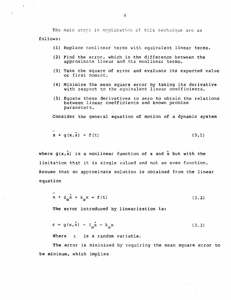
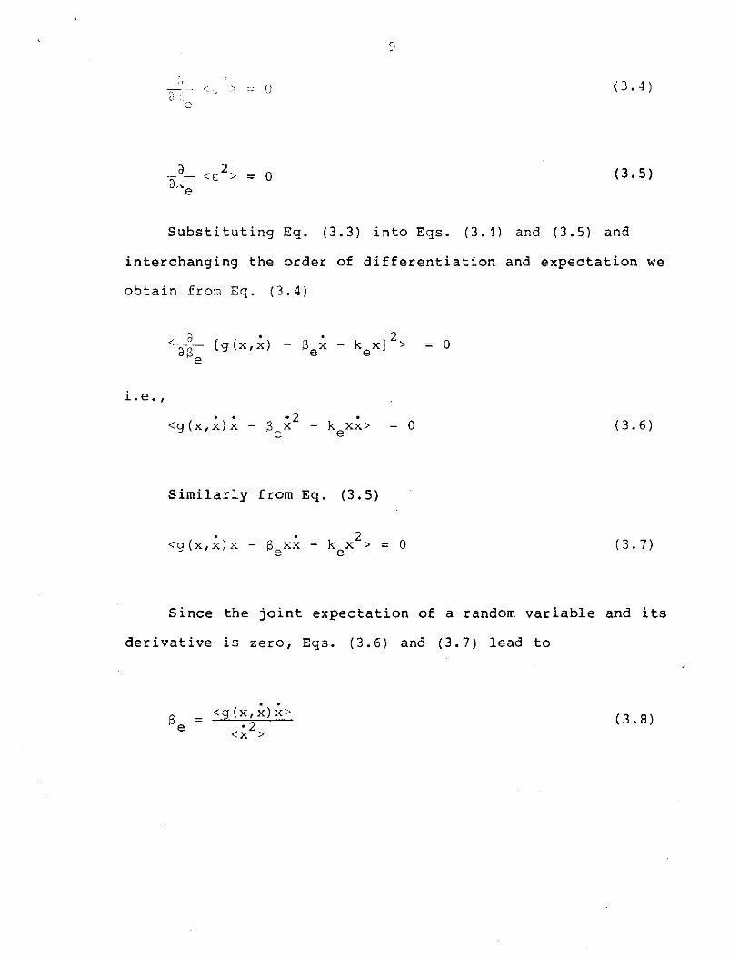
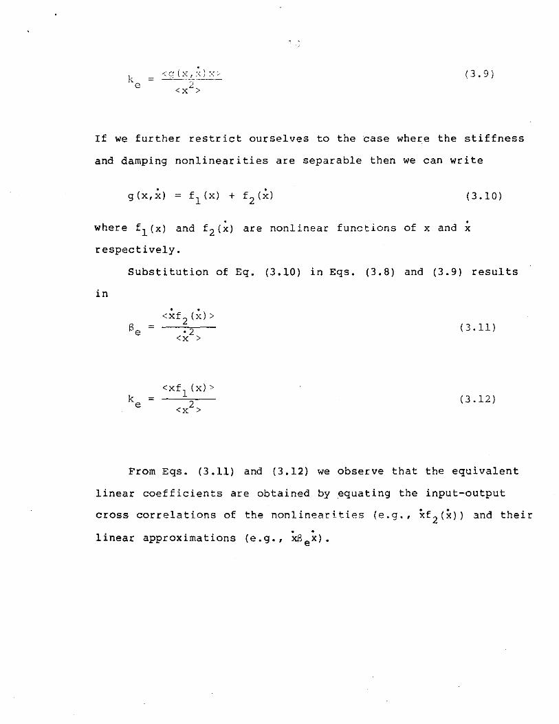
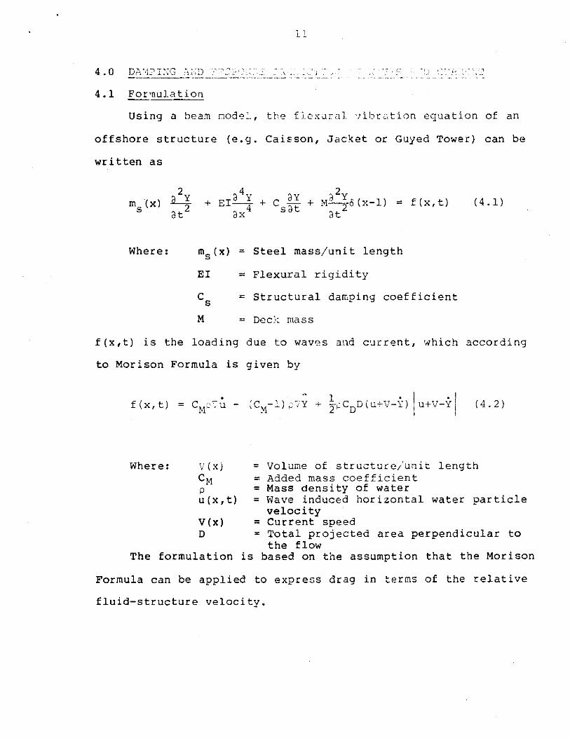
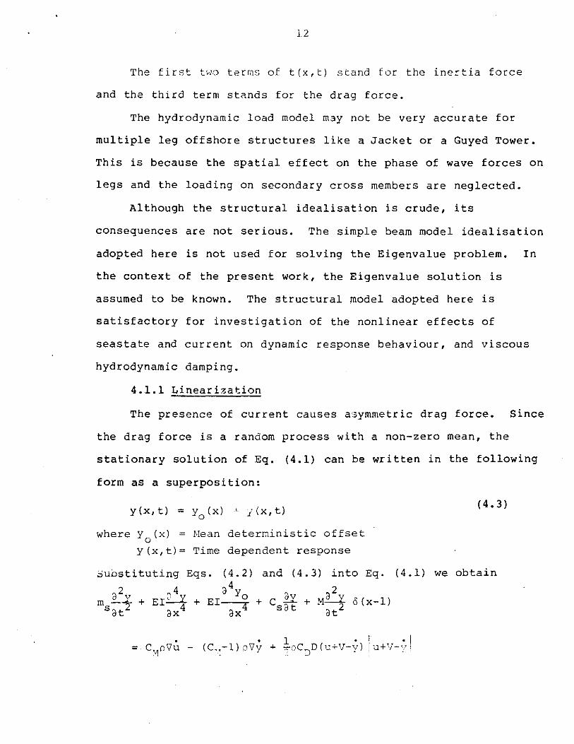
12
The first two terms of t(xt) stand for the inertia force
and the third term stands for the drag force
The hydrodynamic load model may not be very accurate for
multiple leg offshore structures like a Jacket or a Guyed Tower
This is because the spatial effect on the phase of wave forces on
legs and the loading on secondary cross members are neglected
Although the structural idealisation is crude its
consequences are not serious The simple beam model idealisation
adopted here is not used for solving the Eigenvalue problem In
the context of the present work the Eigenvalue solution is
assumed to be known The structural model adopted here is
satisfactory for investigation of the nonlinear effects of
seastate and current on dynamic response behaviour and viscous
hydrodynamic damping
411 Linearization
The presence of current causes asymmetric drag force Since
the drag force is a random process with a non-zero mean the
stationary solution of Eq (41) can be written in the following
form as a superposition
y(xt) = y0
(x) -L j(xt) (43)
where y0
(x) = Mean deterministic offset
y(xt)= Time dependent response
substituting Eqs (42) and (43) into Eq (41) we obtain
2v 4 m ~+EI~+
satL ax4
a4yEI~+
ax~
C f_ sat
2 + M_lt_Y_2at
o(x-1)
bull bull 1 bull I middotI= C~cVu - (C~-l)pVy + ~ocDD(u+V-y) u+V-yi
J __)
This equation can be recast in the following form
4 2 m + EI4 + c zx + MLY_ o(x-1) (CM-l)pVy + c (r)
s sat 2ax at ( 4 4)
Where
( 4 5)g(r) = pc0 o(r+V) jr+vl shy
g(r) is a nonlinear function of r which is the fluid-structure
relative velocity defined as
r = u - y (4 6)
In the stochastic linearization approach g(r) is replaced
by Cer where Ce is the equivalent linear coefficient The
meansquare error between the nonlinear term and its linear
approximation is given by
lt[g(r) - Cer] 2 gt = E ( 4 7)
The equivalent linear coefficient is obtained by equating
the derivative to zero
lt [g(r) - Cer] 2 gt ( 4 8)
Interchanging the order of differentiation and expectation
leads to
lt2[g(r) - C r]rgt = 0 e
= ltCJ(r)rgt ( 4 9)Ce 2 ltr
The quantity ltg(r)rgt is very difficult to evaluate beshy
cause g(r) is related to r in a very complex manner However
the quantity on the right hand side of Eq (49) satisfies
the following Gaussian identity
ltg(r)rgt = ltddr g(r)gt (410)ltr2gt
Proof of this identity is in Appendix A
It turns out that for g(r) as defined in Eq (45) the
right hand side quantity of Eq (410) is far simpler to evaluate
than the left hand side quantity
The equivalent linear coefficient is
Ce= lt~r g(r)gt ( 4 ll)
The equivalent linear coefficient as defined by Eq (411)
is the expected value of the gradient of the nonlinear function
g ( r) bull
Substituting Eq (45) into Eq (411) and carrying out the
differentiation we get
( 4 12)
(r+V) is a non zero mean Gaussian random variable The
quantity lr+vl is evaluated in Appendix B
15
Using the result of Appendix B
v2 Ce = pc D [ ~ or exp(---2 ) + 2VErf (-v__ J (413)
2 D Yi 2or Lor
Where Erf(X) is the Error Function defined as
x Erf(x) = 2 f exp(-t 2 )dt
It is also known as the Probability Integral
or is the rms fluid-structure relative velocity
Spanos investigated the case of a single degree-of-freedom
system under wave-current loading and arrived at similar
expression for the equivalent damping coefficient (Spanos 1981)
Replacing the nonlinear term g(r) with the equivalent linear
term Eq (44) can recast in the following form
4 2()2 [m +(CM-l)p9]~ + EI4 + (C +C ) aYt + MY a(x-L)
s ()t ix s e 0 ()t (414)
From Eqs (413)and (414) we observe that waves and current
influence excitation on the structure as well as damping of the
structure
A component of damping is a function of sea state and
current Similarly there is a sea state and current dependent
exciting force
4 1 2 Solution
The structure response is expressed in terms of its normal
modes centi and generalised coordinates qi
N
y(xtl = I cent(x)q(t) (415)]_ ]_
i=l
For the ith mode the uncoupled modal equation is
Mq + Cq
+ Kq = N ( 4 16) ]_ ]_ ]_ ]_ ]_ ]_ ]_
Where Mi = Modal mass =
L 2 d 2 2f Tl (x)centdx+(C1-l)pf 17ltgtdx + Mcento(x-L0 s ]_ 0 ]_ ]_
ii = Modal stiffness =
2wM ]_ ]_
c ]_
= Modal damping =
+ ~pC fd 2DV Erf(VLcrr)cent~dx2 D i
0
~ = Modal non viscous damping ratio51
d = Depth of water
L = Length of structure
c ]_
(418)=~- = tsimiddot + Evimiddot2Mw ]_ ]_
Where E = Modal viscous damping ratiovi
CD 2 2 2exc(-V 2cr )artax= ]_4Mc ]_ ]_
(4 19)
v Erf (--) o dx]
for i
The modal wave-current induced exciting force is given by
d N 17ZQdx + U [~ f D exp(-V2
2ar2 )crrcentiz~x
]_ ]_ 0 1T ()
(420)d
+ f 2DV Erf (V2crr)Zcentdx]]_
0
In Eq (4 20) the following relations have been used for the
wave induced water particle velocity and acceleration at any
arbitrary depth
(421)
u = u z
0
18
Where u = Wave induced watar particle velocity on the 0
free surface
= Wave induced water particle acceleration on the
free surface
Cosh(kx)z = Depth attenuation factor = Sinh (kd)
k is the wave number
In terms of the modal quantities the variance of the
structural response is
2 cpq) gt
l l (422)
For Caisson or Jacket type offshore structures the natural
frequencies are widely separated and the damping is light
Because of this the responses in different modes can be
considered to be stochastically uncorrelated With this widely
used established hypothesis in structural dynamics the cross
terms on the right hand side of Eq (422) vanish and it
simplifies to
N N2 2 2 2 2 crs = lt I ltP q gt = I ltP crq (423)
l l l li=l i=l
Where cr = rms modal response in the i th modeqi
crs = rms response of structure
1 9
A simple expression for the v3rLance of the relative
fluid-structure velocity can be derived if the cross correlation
between the fluid particle velocity and the structural velocity
is neglected
Nbull 2 2 bull2 bull 2 lt (u-y) gt = ltU gt + lty gt = ltjlJ) gtlt
i=lI l l
In the above expression the cross correlation term has been
neglected
Substituting Eq (423) in this equation leads to
N 2 2 2I ltjloqw (424)l l li=l
wi is the natural frequency corresponding to ith mode
Eqs (419) (420) and (424) indicate that the damping and
excitation in any particular mode depend on the seastate and
responses in all modes This is a manifestation of the nonlinear
drag force
The response spectra of an offshore structure has two types
of peaks One corresponds to the quasi-static response of the
structure and is located at the wave spectral peak frequency
The other type is due to the resonant dynamic response of the
structure at its natural frequencies In this study we are
primarily concerned about low to moderate sea states and hEnce
the quasi-static response is negligible Therefore the response
variance can be computed considering the dynamic response peak
modal response varianc can be estimated by the half power
bandwidth method as follows
i 25Si (CJ) Iw=w
(J 2
l (425)= qi 2 32M1w1s1
Where S ( w) = Spectral density function of modal excitingl force corresponding to i th mode
A compact expression for the modal exciting force can be
written using the two auxiliary variables C and C a u
N = C u + C u (426)i a o a o
Since the fluid particle velocity and acceleration are
stochastically uncorrelated the spectral density function of
modal exciting force is
sl (w) = c 2 s~ (w) + c 2 s (w) (427) a o u uo
Where Su (w) = sdf of fluid particle velocity0
2= CJ S (w)11
suolwJ = sdf of fluid particle acceleration 4
=~s(w) l
S (w) is the sdf of wave elevation 11
Substituting in Eq (427) yields
(428)
Where pCD g d 2 2 c = - -[-- f Dexp (-V 2or ) orcent i Zdx
u 20
d + f 2DV Erf (V2or) cent Zdx]
1 0
21
The mean response of the structure can be determined by
requiring that the solution given by Eq (43) satisfies Eq
(44) on the average
This requirement leads to the following equation
ltg(rgt = 0
(429)
The expected value of the quantity on the right hand side of
Eq (429) has been derived in Appendix C
Substituting the result of Appendix C in Eq (429) leads to
a4y 0 1 2 2 rEI-- = 2pC0D[(V +or )Erf(Vv2or4ax
(430)
+~or exp(-V22or2 ]
This equation is the well known beam equation and the right
hand side quantity is the mean time independent wave-current
induced load It is interesting to note that the mean load is a
function of the sea state in additi0n to current The dependence
on the sea state is caused by the nonlinearity in drag force If
the drag force was linear the mean load would have been a
fun~tion of current 0nly
integration of Eq (4 30) and application of appropriate boundary
conditions
42 Computation
It is apparent from Eqs (419) and (420) that the modal
viscous damping and exciting force depend on the structural
response This necessitates the adoption of an iterative
procedure for the determination of the damping and response
From the computation done in this study it has been observed
that the rate of convergence depends primarily on the response of
the structure When the structural response is small in
comparison to fluid particle motion the rate of convergence is
rapid
The modal quantities given by Eqs (419) and (420) are
evaluated by numerical integration because most of the
quantities in the integrands are not defined analytically For
numerical integration Simpson three point rule is used In the
software developed five equally spaced integration stations are
used over the length of the structure The numerical integration
has the advantage that any arbitrary current profile and mode
shape can be handled These quantities need to be defined
numerically at the discrete integration stations
The d~mping and response prediction is made using the two
parameter Bretschneider wave spectrum defined as 4 4 w w
SLil = 3125 n o~ middotmiddotI --
Where ls = Significant wave height (ft)
w = W2ve frequency correspondina to p spectral peak (radsec)
The peak frequen~y (WP) if not known is estimated in the
following way For Bretschneider spectra the peak frequency is
evaluated using the following relation between the peak frequency
and the average zero crossing period(Tz) (Sarpkaya 1981)
The relation between the significant wave height (Hs) and
the average zero crossing period is proba)ilistic in nature
However for simplicity the following deterministic relation
proposed by Weigel (Weigel 1978) has been used
Tz = 1 723H middot 56 s (432)
Tz is in sec and Hs is in ft
The Error Function in Egs (419) and (420) is approximated
by the following (Abramowitz and Stegun 1965)
Erf(x) = 1 -1 (433)
middotwhere al = 278393
a2 = 230389
a3 = 000972
a4 = 078108
Some other approximations were tried But this particular
one has been found to be well behaved and works better than some
Error Function ie bet~een zero and one
A closed form expression can be derived for the modal
viscous damping when the structural response is negligible
compared to water particle motion This is done for the first
mode of a caisson in this section
Since the structural motion is negligible Eq (424)
becomes
= (J z (434)uo
Where Z is the Depth Attenuation Factor It is assumed that
current V obeys the same Depth Attenuation law This assumption
makes the derivation considerably simpler The choice of current
distribution profile is not crucial Since it has been shown in
the later part of this work that current distribution has
negligible influence on the damping and dynamic response
Based on the assumption made the current speed at any depth
can be expressed as
v = v z 0
Where V0
= Current speed at free surface
Substituting Eqs (434) and (435) in Eq (419) yields
2 2 2[~rd exp(-V 2cr )cr z~dxiVi = 0 uo uo l 0
d + f 2V Z Erf (V 12a ) cjl~dx
0 0 uo l 0
(436)
= Erf (V 2a ) ] 0 uo
(~
x J ZQ~dxl
0
The first mode of a caisson can be approximated by the
following trigonometric function
(437)
Substituting this approximation for the mode shape the
integration in Eq (436) can be evaluated as follows
Calling this integration G(centj we can write
d G ( cent) = f
0
l - i x - exp(---i) - Exp(- -c~) Jdx
2 J L
Performing termwise integration leads to
G(cent)
L2c
kd kdSi nee kdmiddot gt 1 e -1 = e
11d Tid)G (qi) ( 2 k Lcos-L + 2 TI sinr
(4 38)
Further simplification can be achieved when the depth of
water is nearly equal to caisson length ie d=l
Under this condition
3G ( ltjl) = 2k
(439)
The rms fluid particle velocity
H s (440)4
It can be expressed as a function of significant wave height only
by substituting Eq (432) in Eq (440)
Then Eq(440) becomes
2TI HS 4491 H middot (441)0 uo = middot 56 s1723 H x 4 = s
Furthermore
v 78Vc 0 = 44 (442)
H2cruo s
and 2 2v 61V
0 = 0 (443)2 88H2ouo s
For the wave number (K) using the deep water dispersion
relation and Eq (432) leads to
k = 2
w g
= (~)Tz
2 1 g
= g x
4 TI 2
(1 723H s
56 ) 2 = 412 112
HS (444)
Substituting Eqs (441) (442) and (443) in Eq (436)
yields
261V 78V (16 x 91 H ~ 4 exp(- 0
) + 2V Erf( 4 ~)]G(cent)s H bull 88 o H bull s s
= 261V bull 78V
[l 456H ~ exs(----0 ) + 2V Erf( bull 4 ~]s(rJi)s middot H 88 0 11 s s (4 45)
G(cent) which is a function of the mode shape is given by either
Eq (438) or Eq (439)
The wave number (k) which is needed in the evaluation of
G ( q) is given by Eq ( 4 4 4)
Eq (445) provides a means for the prediction of modal
viscous da~~ing of a c2isson in pregtence of waves and current
This equation is not very accurate for the prediction purposes
but it gives a feel for relative influences of different
28
422Fle~ibl~ Ca~son
The Caisson analyzed in this section is located at West
Cameron Block 32 in the Gulf of Mexico It is owned and operated
by Mobil Oil Co The particulars of the Caisson are as below
Total Length = 2300 ft Water Depth = 1750 ft Leg Diameter = Tapers From 16 ft at Mudline to
8 ft at the Waterline Steel Mass = Varies From 18142 slugsft at
Mudline to 2465 slugsft at deck level
Deck Mass = 248450 slugs Natural Frequency = 289 radsec Non viscous Damping = 14 The Caisson is assumed to respond in the first mode only and
the mode shape is shown in Fig2
A sensitivity analysis has been carried out and the
influence of the following engineering parameters on the dynamic
behaviour of the Caisson has been studied
(1) Sea state defined by significant wave height(Hs)
(2) Current speed (V)
(3) Frequency ratio defined as the ratio of the first natural frequency of the structure (wn) and the peak spectral frequency(wp)
(4) Drag coefficient(CD)
(5) Current distribution parameter (Cvgtmiddot This is defined as the ratio of the area under the current distribution profile and the area of the largest rectangle enclosing it A linear profile has a ratio of 12
Figs 4 and 5 show the variatiun of damping and response
with sea state and current speed Damping increases considerably
with current speed and significant wave height The response
increases with sea state (Fig 5) but is hardly i~fluenced by
cmiddoturri~nt
contribute to both e~~itation ar1J d~mping~ T~ercfore the
variation of response ~ith changing sea state or current depends
on the relative magnitudes of modifications in damping and
excitation For the Caisson the response increases with sea
state because the increase in excitation is not fully offset by
the increase in damping Similarly the response increases with
current b8cause the i~=rease in 9xcitati0~ is not fully offset
by the increase in damping due to current
The deck response standard deviation and the modal damping
ratio are plotted agai~st the frequency ratio (wnwp) in Figs 6
and 7 Damping is found to be inversly related to frequency
ratio The plot of response standard deviation vs frequency
ratio resembles the response behaviour of a deterministic dynamic
system under harmonic excitation Like the resonance of a
deterministic system the response standard Jeviation reaches its
peak when the frequency ratio is close to one
In the present analysis a constant drag coefficient has been
used However the drag coefficient is a function of Reynold No
and Keulegan Carpenter No This means that the drag coefficient
is time dependent and also varies along the length of the
structure To find out the consequences of applying a constant
drag coefficient da~ping and response standard deviation have
been plotted against the drag coefficient (C ) in Figs 8 9 100
and 11 The response is found to be rather insensitive to drag
coefficient The damping increases with the drag coefficient
30
distribution i13~e ne0ligi~le effects on darriping and response
423 Guved Tower
In this section the results of an analysis for a Guyed
Tower are presented The purpose here is not to predict the
design values but to present characteristic response quantities
The relative significance of some important environmental and
structural parameters is investigated and some specific
conclusions drawn
A Guyed Tower is a compliant structure (Fig 13) The guy
lines provide the soft restoring force The tower is essentially
a truss work built between four corner legs The tower rests on
a piled foundation The tower base can be idealised to be free
to rotatebut fixed against sliding
The particulars of the specific tower considered are
given below
Total Length = 18040 ft
Water Depth = 16892 ft
Leg Diameter = 656 ft
Steel Mass = 5300 slugsft
Deck Mass = 3742940 slugs
Sway Mode Natural Frequency = 20 radsec
Bending Mode Natural Frequency = 14 radsec
Bending Mode Non Viscous Damping = 20
The first two natural modes of vibration are shown in Fig
14 In the present analysis it is assumed that the tower
~- --middot -middot middot middot-middot
middot J
rotation and the response i1 this mode is determined by the tower
mass and guy stiffness This is referred to as the sway mode
The response in the second mode called the bending mode here is
dictated by the tower mass and flexural stiffness
The response in the sway mode is not computed here This
mode is primarily excited by the second order wave forces and
wind forces both of which are difficult to model in the
frequency domain in spectral terms The standard deviation of
the sway mode response is input as a known quantity
The two quantities that have been predicted are the viscous
damping ratio and the standard deviation of deck response in the
bending mode The second response quantity is by itself not very
important because the deck response is primarily caused by the
sway mode However the deck response in the bending mode is a
measure of the tower bending moment Because the standard
deviation of bending moment is directly proportional to the
standard deviation of displacement response
The influence of the following parameters on the bending
mode response has been investigated
(1) Significant wave height (Hs)
(2) Current speed (V)
(3) Standard deviation of dee~ response in the sway mode ( J s )
37
(4) Ratio of benJinJ soJe natural frequency and frequency (_ middotmiddot- middot)of somiddot~-cl - - l- - -~ bullmiddotmiddotmiddot rt ~ p
(5) Current distribution parameter (Cy) which has already been defined
(6) Drag coefficient (C0 )
The sway mode motion influences the damping and excitation in the
bending mode through Eq (424)
Examination of Figs 15 16 17 18 19 20 reveals that the
damping in the bending mode is very sensitive to current and the
sway mode response but very little influenced by the sea state
This is because wave induced water particle velocity attenuates
v-dry rapidly in moderate sea states It is predominant near the
free surface Therefore the standard deviation of relative
fluid-structure velocity (Or) and the equivalent damping
coefficient are dominated by the sway mode response and ocean
current The response in the bending mode increases initially
with significant wave height (Figs 16 18 20) but then flattens
out for high sea states This is probably because the spectral
peak frequency moves away from the bending mode natural frequency
as the significant wave height goes up
Although the standard deviation of bending mode response
decreases with increasing current (Fig 16) the
rms response will not necessarily follow the same trend
Because the rms value depends on mean deflection which
increases with current (Eq 430)
In Figs 22 and 24 the bending mode response standard
deviation has been plotted against the frequency ratio The
resonance like effect is noticeable here also li~e tl1e Caisson
From Fig 25 it is observed that damping increases and
response decreases as the variation of current with depth gets
more uniform
In Fig 26 damping and response are plotted against drag
coefficients Unlike the caisson damping increases and response
decreases with increasing drag coefficients
)
50 c)1 -middotmiddotmiddot --middot- -middot ___middot~
A simple approach based on the Stochastic Linearization
technique has been presented for the dynamic response analysis of
offshore structures excited by waves and current Because of
the presence of current the drag force is asymmetric
Consequently the stationary solution for structural response
consists of superposition of a time independent deterministic
offset and a randomly fluctuating component The main focus in
this study has been on the randomly fluctuating component of
response But the equation for deterministic offset has been
derived
The Stochastic Linearization technique replaces the original
nonlinear drag term with an equivale~t (optimal) linear drag
term The equivalent linear equation has been employed with an
iterative numerical scheme to obtain an approximate solution for
the standard deviation of response of the original nonlinear
system
Parametric studies have been conducted on a stiff shallow
water structure and a compliant deep water structure These
studies have helped to gain insight into the dynamic behaviour of
offshore structures Also based on these studies some general
comments can be made For shallow water structures sea state
appears to have the most significant influence on the dynamic
response ot the structure On the other hand for deep water
compliant structures the dynamic behaviour in the bending mode
depends primarily on the compljant mode response and the ocean
response in the compliant mode For deep water compliant
structures the response in the bending mode depends heavily on
the drag coefficient value Therefore a judicious selection of
drag coefficient is important
36
6 0 REFERECE~~
(1) Abramowitz M and Stegun IA Handbook of Mathematical Functions Dover New York 1963
(2) Booton RC The Analysis of Nonlinear Control Systems with Random Inputs IRE Trans Circuit Theory Vol 1 1954
(3) Brouwers JJH Response Near Resonance of Nonlinearly Damped Systems Subject to Random Excitation with Application to Marine Risers Ocean Engineering Vol 9 No3 1982
(4) Crandall SH Perturbation Technique for Random Vibrations of Nonlinear Systems J of Acoustical Society of America Vol 35 1963
(5) Dunwoody AB The Role Separated Flow in the Prediction of the Dynamic Response of Offshore Structures to Random Waves Doctoral Thesis MIT 1980
(6) Foster ET Semilinear Random Vibration in Discrete Systems J of Applied Mechanics Vol 35 1968
(7) Iwan WD Yang I Application of Statistical Linearization Techniques to Nonlinear Multi-deg-of-freedom Systems J of Applied Mechanics Vol 39 1972
(8) Iyenger RN Random Vibration of a Second Order Nonlinear Elastic System J of Sound and Vibration Vol 40 No 2 1975
(9) Lin YK Probabilistic Theory of Structural Dynamics Robert E Krieger Publishing Co New York 1976
(10) Rajagopalon A Dynamics of Offshore Structures Part 2 Stochastic Averaging Analysis J of Sound and Vibration Vol 83 No 3 1982
(11) Spanos PD Chen TW Random Response to Flow-Induced Forces J of Engineering Mechanics Div ASCE Vol 107 No EM6 1981
(12) Taylor RA Rajagopalon A Dynamics of Offshore Structures Part l Preturbation Analysis J of Sound and Vibration Vol 83 No 3 198
(13) Volterra V Theory of Functional and of Integral and Integro Differential Equations Blackie and Sons Ltd London 1930
- 1( 14) - -- I Dmiddot~~i~n Spectra 11
Co1middot middot 1 r~middot11middot--isLty o[ Cal fornia B~rkeley 1978
(15) Wiener N Nonlinear Problems in Random Theory The Technology Press of MIT and John Wiley and Sons Inc New York 1968
Proof of Gaussian Identity
ltg(r)rgt = lt~ g(r)gt ltr2gt dr
By definition
100 dg(r) p(r) drlt~r g(r)gt = dr -oo
where
p(r) = Gaussian probability density function for the random variable r
1 2 2 = exp (-r 2crr ) (A l) 21lrr
Integrating by parts
00
lt~ g(r)gt = p(r)g(r) loo I dp(r) g(r)drdr dr -oo-oo
Taking derivative of p(r) and substituting
lt~ g(r)gt = -loo g(r) C-rI crr 2 )p Cr)drdr -oo
00 ltrg(r)gt= --17 1 r g(r)p(r)dr = 2 00 gtor - ltr
38
-oo
lltlr+VIgt = 00
lr+vl p(r) dr = -oo arl2n
-v 2 2 00 2 l = --- [- (r+V)exp(-r 2ar )lr + f (r+V)exp(-r 2ardr]
arl2iT -oo -v
(B 1)
00 ~) ] 7 = _1__ [2 middot- ex~(-r~2Jr-)dr+2V exp(-r- ar~middot v 0
l = ar~
middot~
Evaluation of lt2lr+VIgt
The expected value of a function of a random variable can
be computed without first determining the complete probability
structure of the function provided the function is a Borel
function For our purposes it suffices to know that a function
with atmiddotmost a finite number of discontinuities is a Borel
function
Assuming that lr+vl is a function of r which satisfies
such properties we can write
Breaking up the limits of the second integration we have
-v 2 2 -v 2 2 ltJr+vlgt =
l [ - f exp(-r 2ar ) - f exp(-r 2ar )dr arl2iT -oo -oo
vv 2 2 2 2 + f Vexp(-r 2ar ~r + f r exp(-r 2ar )dr
-v -v
00 002 2 2 2+ f V ~xp(-r 2ar ~r + f r exp(-r 2ar )dr] (B 2)
v v Application of properties of even andodd function leads to
n
ll = r exp(-r22or2 )dr (B 4) v
and
12 = v exp (-r22or2 )dr 0
Breaking up the limits of integration for 1 we have 1
2 2 v 2 2 r exp(-r 2or )dr - r exp(-r 2or )dr
0 (B4)
For the first integration in (B4) the following integration
result is used
f 00 2 2 nlt n+l exp (-at )dt =
2an+l0
and we have
1 2 2 2 - (-or ) exp (-r 2or ) 2 (-1-) 022or
Iv
2 2 2= or exp (-V 2or ) (B 5)
1 is evaluated using the following result2
u 2 2 ITexp(-q x ) dx Erf(qu) = 2q0
TI Erf (V12or) 212or
(B 6)
Substituting Eqs (B5) and (B6) in Eq (B3)
1 2 2 2ltI r+vl gt = [2or exp(-V 2or ) or2iT
+ 2V orliT Erf(V12or) l 12
2 2= ~ Ii or exp(-V 2or ) + VErf(V12or)
Finally
2 2lt2lr+vlgt = ~or exp(-V 2or ) + 2 VErf(V12or)1T
~ l
= [4Vf r exp(-r 2crr )dr orl2 r ~r
Evaluation of lt(r+V) lr+vgt
Following the same arguments as in Appendix B
00
lt(r+V) lr+VIgt = f (r+V) lr+Vip(r)dr -oo
-v1 2 2 2= --- [ - f (r+V) exp(-r 2crr )dr crr21T -oo
00
2 2 2+ f (r+V) exp(-r 2crr )dr] -v
-v1 2 2 2 v 2 2 2 = [ middot- f V exp(-r 2crr )dr - f r exp(-r 2crr )dr
crrl2if -oo -v
-v v2 2 2 2 2 - 2Vf r exp(-r 2crr )dr + f v exp-r 2crr )dr
-oo -v
v 2 v2 2 2 2 + f r exp(-r 2crr )dr + 2Vf r exp(-r 2crr )dr
-v -v
00
2 2 2 2 2 2+ f v exp(-r 2crr )dr + 00
r exp-r 2crr )dr v v
2 2+ 2Vf r eXF(-r 2crr )dr] v
1 00
2 2
00
arlIT 2 2 2Erf VvLcrr) - 2Vcrr exp-V 2crr l
12
+ 2ar2 arlIT Erf V2crr) l 12
22Var 2 2 2ar2rrr ) Erf (V12crr)= exp-V 2crr ) + 2V 11 + 1211 Frroshy
=rTv 1[
middot1 3
2v 2 2 v2 2 2 +2V exp-r 2crr )dr + 2 r exp-r 2crr )dr] (c 1)
0 0
The first two integrations in Cl) are already evaluated in
Appendix B and the third integration is evaluated as follows
vv 2 2 2 2 2 r exp-r 2crr )dr = rr exp-r 2crr dr)) j I0
0
v 2 2 2 - - ar exp-r 2crr )dr 0
= -ar2 V exp-v22crr2 ) + ar2 arTI Erf(V12crr) 12
Substitution of this result and results of Appendix B in
Eq Cl) leads to
1 2 2 2 lt r+V) Ir+V Igt = [4Vcrr exp-V 2crr ) +
arl2iT
y
~~It I CAI~SON
------
SiiAi E
-------
------Vmiddot 2middoto Ft5ec
___--YbulllmiddotO Ft b-ec 1middot0 ------------ v =o R gt
ee
4middot0 Smiddoto J2middot0 Hs (F-l)
FIG4 SIGNIFICANT WAVE HEIGliT CHs) VS
j - L
4middoto-
V=O 20 shy -~Vbull2middot0
I I I
4-o Bmiddoto 12middot0
FIG5 DCCIlt RESPONSE STD DEVIATION CltJd_) VS
SIGNIFICANT 1AAVE HEIGHT CJ-15 )
2middot0
5v c )
1-o
middotso 1middot6o 2middot4o U)p FI 6 MODAL VIGCY DAMPillG RATIO C~V gt
vs FrraufrY RATIO C(i)nj) Igt
Zo
a4(Ft) ~ lmiddoto
middotao
FIG 7 DCCK RESP01~iSE STD DEVIATION CC5f gt
VS FREQUENCY RATIO C~~traquof
v o r-tsec2middoto
5v (1)
lmiddoto
bull80 lmiddotoo
FIGS MODAL VISCOUS DAN~ING RATIO C~y)
2middoto Y =o Rs~c
lbullo ------ ~= Bmiddoto ~~~~~~-~sbull4o
middoteo lmiddotoo
FIG9 DE~K RESPONSE STD DEVIATION CQd)
Hs = 4middot0 Ft
I middoto ------Vlmiddoto - V=o
80 lbullOO 1middot2o Cp
FIG 1~ ~cmiddoto~L VT~~cus DAMPIN~ RATIO ~v)
V~ DkA~ COEFFICIENT CY)
2middot0
6d(=t) lbullO
=============Yeo Ybulllmiddoto
middoteo lmiddotoo 1middot2o Co
FIG 11 DECK RESPONSE STD DEVIATION C 6J)
VS DRAG CDEFfICIENT CCD)
2middoto Hb =4middoto Ft Y = Imiddot o Ftlt$c5v Ct)
lmiddotoJmiddoto-+ ------~v Od
40 6o iO Cv
50
FIG12 MODAL YISCCUs 0AMPIN RATIO C1Sv)
AND DC2K ~ESFCN5E STD DEVIt TICN C 6d)
VS CURRENT DISTRIBUTION PARAMETER CCv)
iflDING SA Y MODE
MCDE
FIG14 TOER MODE SHAPESFIG 13 GUYED TOER
o = middot5 4middoto
-------Vbull2middoto
-------Vbulllmiddoto
------- v =-0
4middoto 8middoto 12middoto Hs (Ft)
VS SINii--ICANT JAVE HEIGHT CHs)
I I I
-
-
------V=o
~-V=lmiddoto -~------y 30 --
I I I
4middoto 8middoto 12middot0
FIG 16 DECK RESPONSE STD DEVIATION C Qb)
VS SIGNIFICANT lAVE HEIGHT CH5 )
os is given as a percentage of tower length
V=-o Fts~c -------o =1bull54o
------6$=1middot0
------deg5=middot5
4middoto 8middoto
FTG17 MOLlL VTobull_is DAf~~ING RATIO C~y)
VS SIGNIFICANT ~AVE HEIGHT CHs)
4middot0 Bmiddoto
FIG18 DECK RESPONSE STD DEVIATION C6b)
VS SIGNIFICANT ~AVE HEIGHT CH~)
4middoto
-------6= Imiddot omiddott
-------66bull5
4middoto 8middot0 12middot0
VS SIGNIFICANT WAVE HEIGliT C Hs)
V = middot o =t- fgtec
4middot0 Bmiddoto
FIG2~ DEeK RESPONSE STD DEVIATION C6h)
VS SIGNIFICANT YAVE HEIGHT CH5)
4middot0
~--- 1-b s Bmiddoto ~----- Hs = 4middoto
I middoto 1middot2 Imiddot 40
FI~21 NODAL VISC~US DAMPIN~ RATIO C~y)
-3 i110 H6 8middoto
VQ
6~ middots 1shy
H~ 4middoto
middot lmiddoto 1middot2
FIG 22 DECK RESPONSE STD DEVIATION C61-)
VS FR~OUENCY RATIO C~~) tgt
V _Imiddot o FtSee 6$ = 5 jl
---- H~ 8 middoto
Hs = 4middoto
lmiddoto Imiddot 2
FI~23 MOD~L VIS~OUS DAMPING RATIO C~v)
V~ FREQUENCY RATIO CQ1~
V =lmiddoto Ft~ec 66bull5
4middot03l o-
cb(rt)
lmiddoto 1middot2o
5G
FIG 24 DECK RESPONSE STD DEVIATIOll Cob)
VS FREQUENCY RATIO C~j~
4middoto
3v ()2middoto
H6 4middot o l=t V lmiddoto rt~c ()~ middot5t ~-----iv
Ob
-34middoto gtltlo
0-b (Fi)2middot0 XI o-3
4o middot~o Cv
DAMPTN~ RATIO C~vl
AND DECK RESPONSE STD DEVIATION C6bl
VS CURRENT DISTRIBUTION PARAMETER CCvl
4middoto
61(r=t)
2middoto 2middoto o-3
tmiddoto 1middot2o
FIG26 MODAL VISCOUS DAMPING RATIO C~yl
VS DRAG COEFFICIENT CC~)
bullI
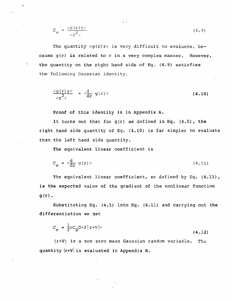
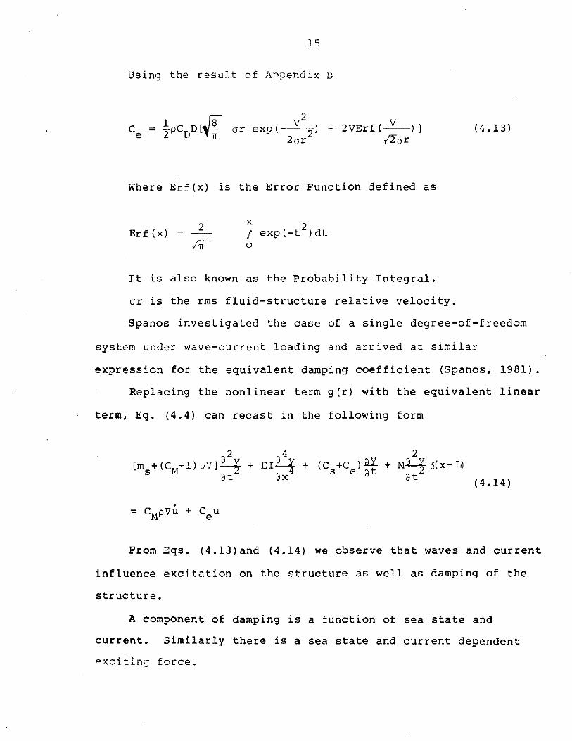
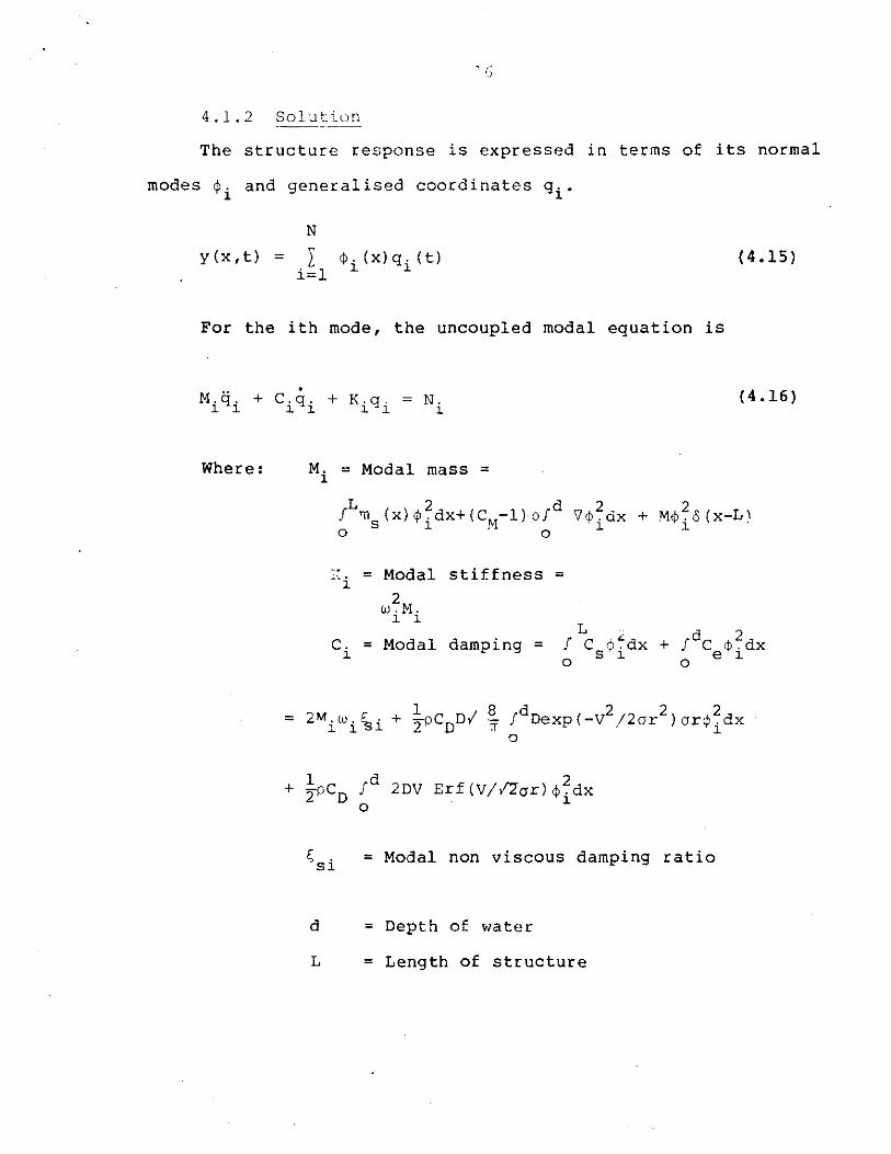
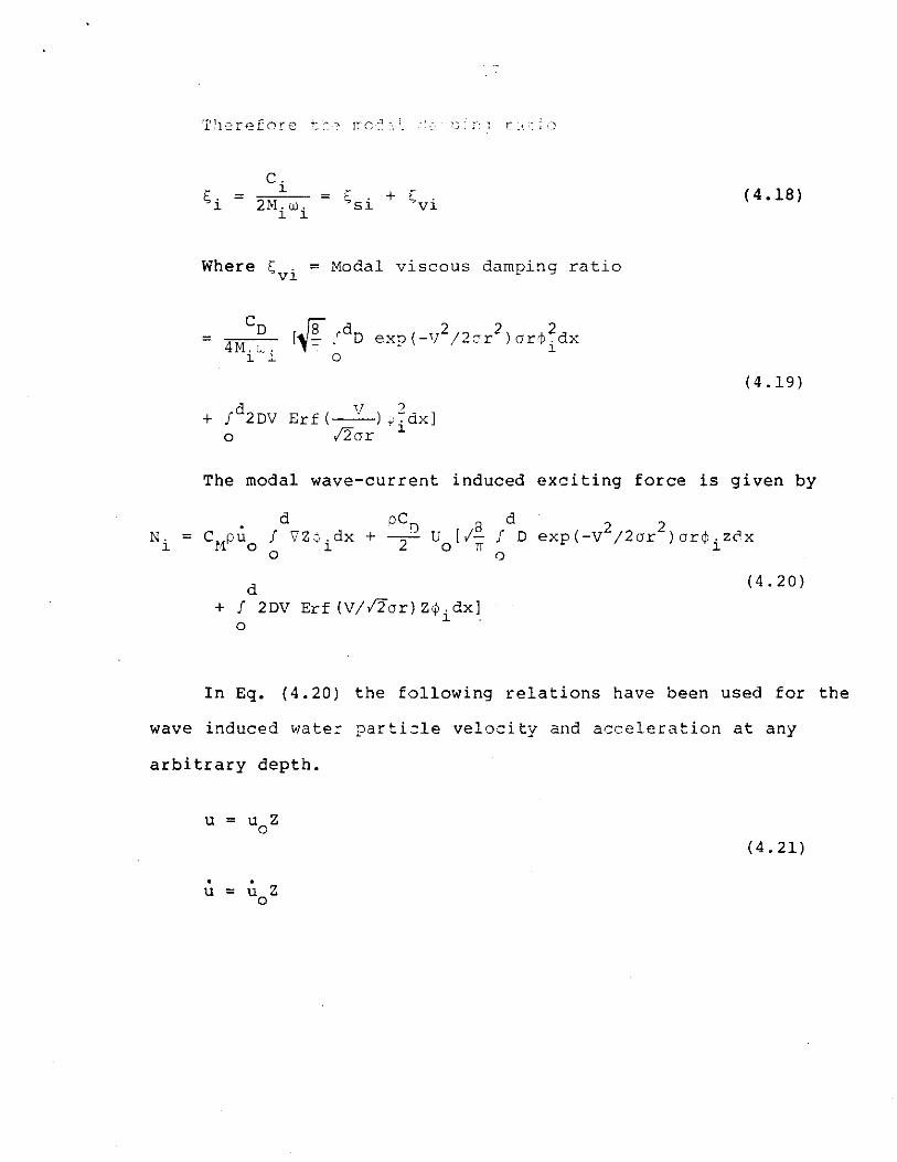
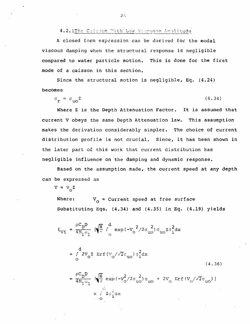
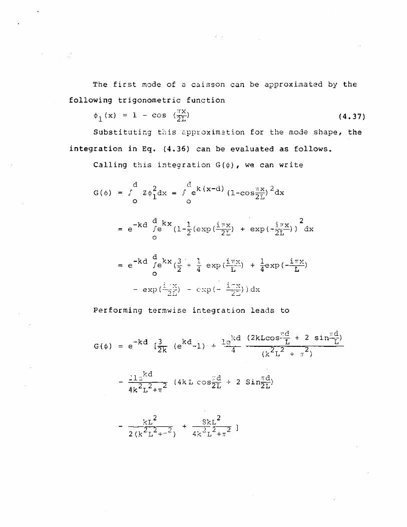
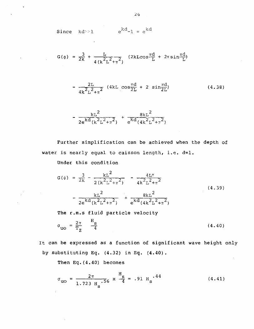
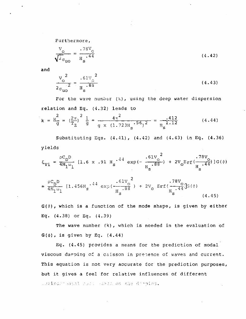
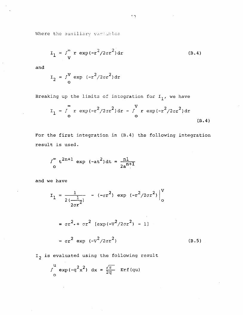
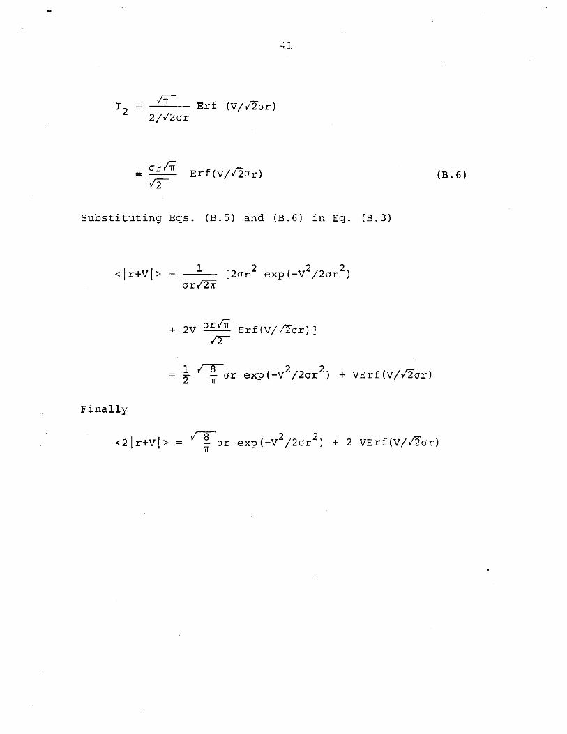
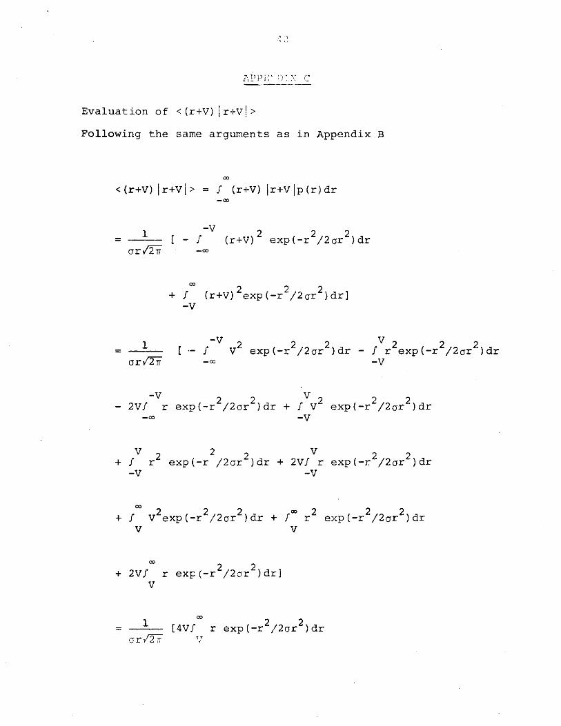
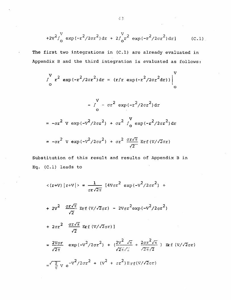
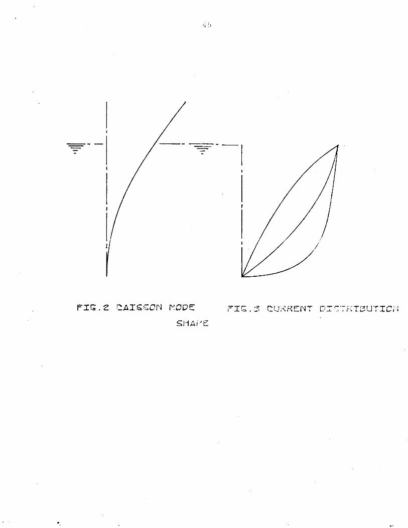
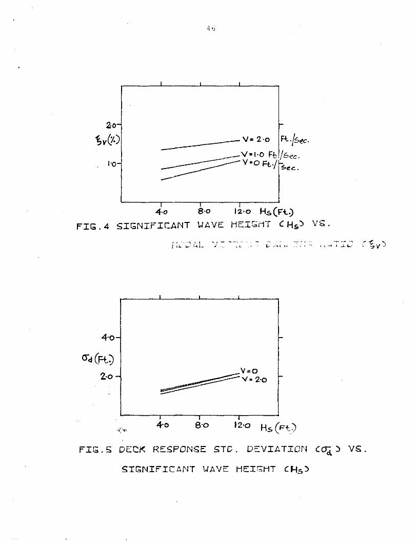
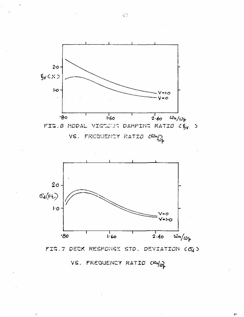
2middot0
5v c )
1-o
middotso 1middot6o 2middot4o U)p FI 6 MODAL VIGCY DAMPillG RATIO C~V gt
vs FrraufrY RATIO C(i)nj) Igt
Zo
a4(Ft) ~ lmiddoto
middotao
FIG 7 DCCK RESP01~iSE STD DEVIATION CC5f gt
VS FREQUENCY RATIO C~~traquof
v o r-tsec2middoto
5v (1)
lmiddoto
bull80 lmiddotoo
FIGS MODAL VISCOUS DAN~ING RATIO C~y)
2middoto Y =o Rs~c
lbullo ------ ~= Bmiddoto ~~~~~~-~sbull4o
middoteo lmiddotoo
FIG9 DE~K RESPONSE STD DEVIATION CQd)
Hs = 4middot0 Ft
I middoto ------Vlmiddoto - V=o
80 lbullOO 1middot2o Cp
FIG 1~ ~cmiddoto~L VT~~cus DAMPIN~ RATIO ~v)
V~ DkA~ COEFFICIENT CY)
2middot0
6d(=t) lbullO
=============Yeo Ybulllmiddoto
middoteo lmiddotoo 1middot2o Co
FIG 11 DECK RESPONSE STD DEVIATION C 6J)
VS DRAG CDEFfICIENT CCD)
2middoto Hb =4middoto Ft Y = Imiddot o Ftlt$c5v Ct)
lmiddotoJmiddoto-+ ------~v Od
40 6o iO Cv
50
FIG12 MODAL YISCCUs 0AMPIN RATIO C1Sv)
AND DC2K ~ESFCN5E STD DEVIt TICN C 6d)
VS CURRENT DISTRIBUTION PARAMETER CCv)
iflDING SA Y MODE
MCDE
FIG14 TOER MODE SHAPESFIG 13 GUYED TOER
o = middot5 4middoto
-------Vbull2middoto
-------Vbulllmiddoto
------- v =-0
4middoto 8middoto 12middoto Hs (Ft)
VS SINii--ICANT JAVE HEIGHT CHs)
I I I
-
-
------V=o
~-V=lmiddoto -~------y 30 --
I I I
4middoto 8middoto 12middot0
FIG 16 DECK RESPONSE STD DEVIATION C Qb)
VS SIGNIFICANT lAVE HEIGHT CH5 )
os is given as a percentage of tower length
V=-o Fts~c -------o =1bull54o
------6$=1middot0
------deg5=middot5
4middoto 8middoto
FTG17 MOLlL VTobull_is DAf~~ING RATIO C~y)
VS SIGNIFICANT ~AVE HEIGHT CHs)
4middot0 Bmiddoto
FIG18 DECK RESPONSE STD DEVIATION C6b)
VS SIGNIFICANT ~AVE HEIGHT CH~)
4middoto
-------6= Imiddot omiddott
-------66bull5
4middoto 8middot0 12middot0
VS SIGNIFICANT WAVE HEIGliT C Hs)
V = middot o =t- fgtec
4middot0 Bmiddoto
FIG2~ DEeK RESPONSE STD DEVIATION C6h)
VS SIGNIFICANT YAVE HEIGHT CH5)
4middot0
~--- 1-b s Bmiddoto ~----- Hs = 4middoto
I middoto 1middot2 Imiddot 40
FI~21 NODAL VISC~US DAMPIN~ RATIO C~y)
-3 i110 H6 8middoto
VQ
6~ middots 1shy
H~ 4middoto
middot lmiddoto 1middot2
FIG 22 DECK RESPONSE STD DEVIATION C61-)
VS FR~OUENCY RATIO C~~) tgt
V _Imiddot o FtSee 6$ = 5 jl
---- H~ 8 middoto
Hs = 4middoto
lmiddoto Imiddot 2
FI~23 MOD~L VIS~OUS DAMPING RATIO C~v)
V~ FREQUENCY RATIO CQ1~
V =lmiddoto Ft~ec 66bull5
4middot03l o-
cb(rt)
lmiddoto 1middot2o
5G
FIG 24 DECK RESPONSE STD DEVIATIOll Cob)
VS FREQUENCY RATIO C~j~
4middoto
3v ()2middoto
H6 4middot o l=t V lmiddoto rt~c ()~ middot5t ~-----iv
Ob
-34middoto gtltlo
0-b (Fi)2middot0 XI o-3
4o middot~o Cv
DAMPTN~ RATIO C~vl
AND DECK RESPONSE STD DEVIATION C6bl
VS CURRENT DISTRIBUTION PARAMETER CCvl
4middoto
61(r=t)
2middoto 2middoto o-3
tmiddoto 1middot2o
FIG26 MODAL VISCOUS DAMPING RATIO C~yl
VS DRAG COEFFICIENT CC~)
bullI
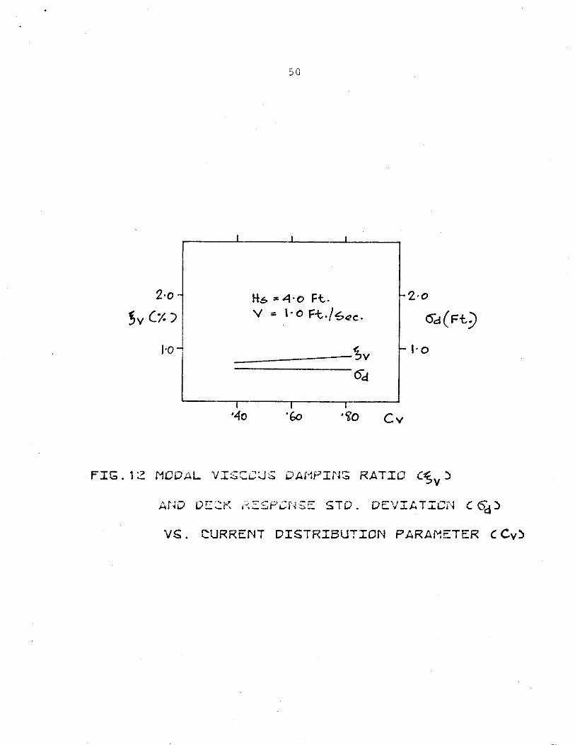
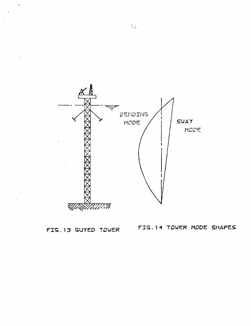
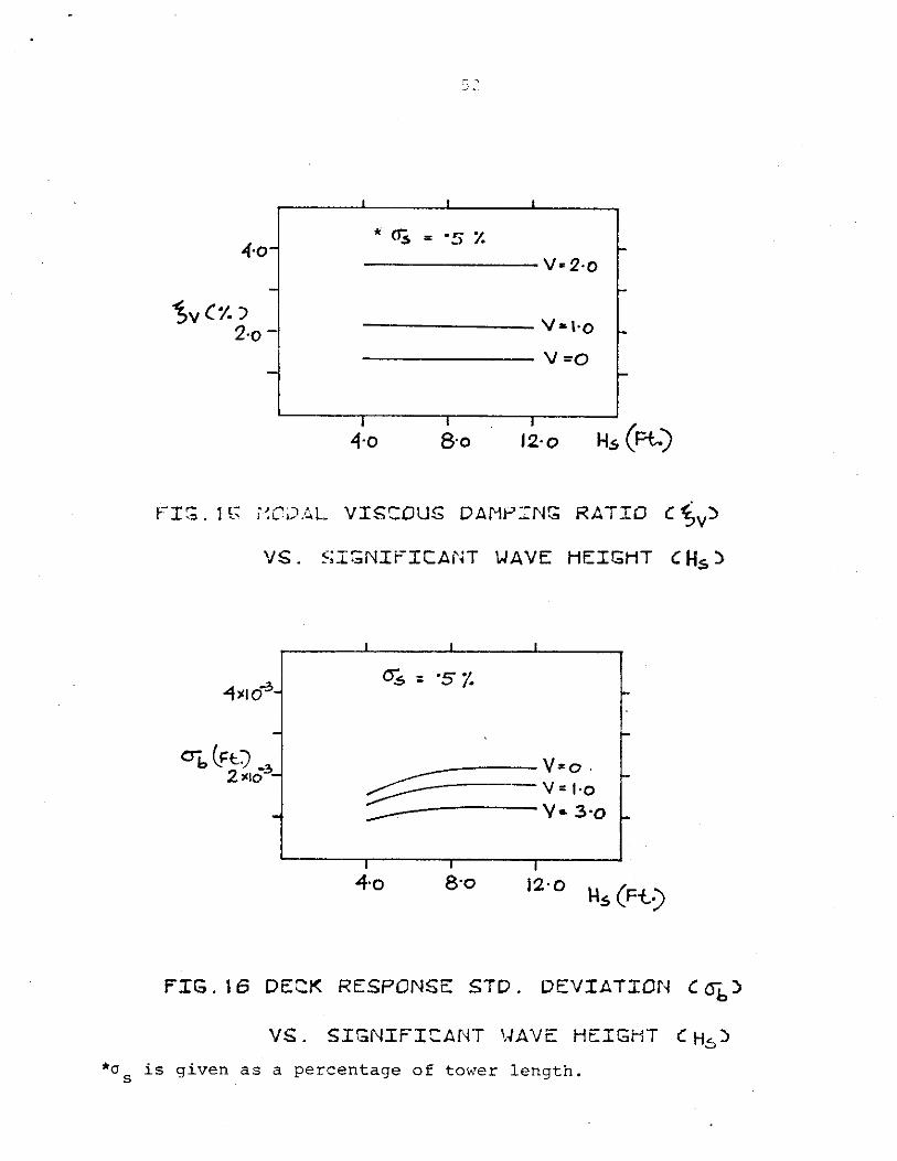
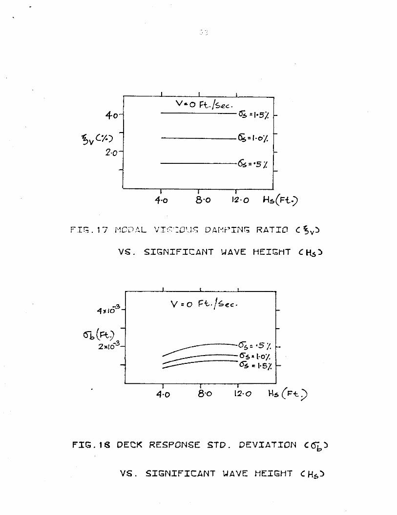
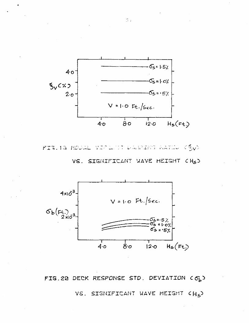
4middoto
-------6= Imiddot omiddott
-------66bull5
4middoto 8middot0 12middot0
VS SIGNIFICANT WAVE HEIGliT C Hs)
V = middot o =t- fgtec
4middot0 Bmiddoto
FIG2~ DEeK RESPONSE STD DEVIATION C6h)
VS SIGNIFICANT YAVE HEIGHT CH5)
4middot0
~--- 1-b s Bmiddoto ~----- Hs = 4middoto
I middoto 1middot2 Imiddot 40
FI~21 NODAL VISC~US DAMPIN~ RATIO C~y)
-3 i110 H6 8middoto
VQ
6~ middots 1shy
H~ 4middoto
middot lmiddoto 1middot2
FIG 22 DECK RESPONSE STD DEVIATION C61-)
VS FR~OUENCY RATIO C~~) tgt
V _Imiddot o FtSee 6$ = 5 jl
---- H~ 8 middoto
Hs = 4middoto
lmiddoto Imiddot 2
FI~23 MOD~L VIS~OUS DAMPING RATIO C~v)
V~ FREQUENCY RATIO CQ1~
V =lmiddoto Ft~ec 66bull5
4middot03l o-
cb(rt)
lmiddoto 1middot2o
5G
FIG 24 DECK RESPONSE STD DEVIATIOll Cob)
VS FREQUENCY RATIO C~j~
4middoto
3v ()2middoto
H6 4middot o l=t V lmiddoto rt~c ()~ middot5t ~-----iv
Ob
-34middoto gtltlo
0-b (Fi)2middot0 XI o-3
4o middot~o Cv
DAMPTN~ RATIO C~vl
AND DECK RESPONSE STD DEVIATION C6bl
VS CURRENT DISTRIBUTION PARAMETER CCvl
4middoto
61(r=t)
2middoto 2middoto o-3
tmiddoto 1middot2o
FIG26 MODAL VISCOUS DAMPING RATIO C~yl
VS DRAG COEFFICIENT CC~)
bullI
4middoto
3v ()2middoto
H6 4middot o l=t V lmiddoto rt~c ()~ middot5t ~-----iv
Ob
-34middoto gtltlo
0-b (Fi)2middot0 XI o-3
4o middot~o Cv
DAMPTN~ RATIO C~vl
AND DECK RESPONSE STD DEVIATION C6bl
VS CURRENT DISTRIBUTION PARAMETER CCvl
4middoto
61(r=t)
2middoto 2middoto o-3
tmiddoto 1middot2o
FIG26 MODAL VISCOUS DAMPING RATIO C~yl
VS DRAG COEFFICIENT CC~)
bullI


![I. Engineering Property Prediction Tools for Tailored Polymer ......concentrated suspensions. This term hence depicts the hydrodynamic interactions. Later, Advani and Tucker [10] recast](https://img.pdfslide.net/doc/110x75/60cbcb1364cacb3bd1272be9/i-engineering-property-prediction-tools-for-tailored-polymer-concentrated.jpg)


![Hydrodynamic fluctuations and Stokes' law friction · Landau and Lifshitz [5]. In the Landau-Lifshitz theory, as applied to a viscous incompressible fluid at low Reynolds number,](https://img.pdfslide.net/doc/110x75/5b395d807f8b9a4a728e18cb/hydrodynamic-fluctuations-and-stokes-law-friction-landau-and-lifshitz-5.jpg)