The Prediction of Permeability for an Epoxy/E-Glass

INTRODUCTION

Fluid flow in Liquid Composite Molding (LCM) proc-esses such as resin transfer molding (RTM) is

usually modeled using Darcy’s Law, given by

(1)

where v is the average (superficial) velocity in themedium, P is the pressure, K= is a symmetric, secondorder tensor known as the permeability and � is thefluid viscosity. Darcy’s law is a volume-averaged modelin which all the complicated interaction that takesplace between the fluid and the fiber preform struc-ture is accounted for through the permeability. Ac-curate permeability data, therefore, are a critical re-quirement if a priori modeling efforts based on Darcy’slaw are to be successfully used in the design and opti-mization of these processes. Currently, the most reli-able and commonly used technique for obtaining per-meability values is via experimental measurements in

v � �K��

# §P

The Prediction of Permeability for anEpoxy/E-glass Composite Using

Optical Coherence Tomographic Images

JOY P. DUNKERS*, FREDERICK R. PHELAN, CARL G. ZIMBA,KATHLEEN M. FLYNN, DANIEL P. SANDERS,

RICHARD C. PETERSON, and RICHARD S. PARNAS†

Polymers DivisionNational Institute of Standards and Technology

100 Bureau Dr.Gaithersburg, MD 20899

XINGDE LI and JAMES G. FUJIMOTO

Department of Electrical EngineeringMassachusetts Institute of Technology

Cambridge, MA 02139

Knowledge of the permeability tensor in liquid composite molding is important forprocess optimization. Unfortunately, experimental determination of permeability isdifficult and time consuming. Numerical calculation of permeability from a model re-inforcement can circumvent experimentation. However, permeability predictionsoften rely on a model reinforcement that does not accurately mimic the actual mi-crostructure. A rapid, nondestructive technique called optical coherence tomography(OCT) can image the microstructure of a composite in minutes. Actual microstruc-tural information can be then used to improve the accuracy of the model and there-fore the predicted permeability. Additionally, the influence on fiber volume fractionand microstructural variability on permeability can be systematically studied.

In this work, binary images were generated from the low contrast OCT datathrough image de-noising, contrast enhancement and feature recognition. The re-sulting data were input to a lattice-Boltzmann model for permeability prediction. Theinfluence of the fiber volume fraction, tow surface area, average mean free channelpath, and variable microstructure are discussed in terms of their individual andsynergistic effects on permeability. The calculated axial and transverse permeabili-ties from the images show very good agreement with the experimental values.

POLYMER COMPOSITES, DECEMBER 2001, Vol. 22, No. 6 803

*Corresponding author.†Present address: Institute of Materials Science,University of Connecticut, Storrs, CT 06269.

either radial or unidirectional flow configurations (1).However, experimental characterization is slow, as itinvolves a large number of carefully controlled experi-ments over a large range of volume fractions. Anothermore serious limitation is that it is difficult to conductexperiments on the materials in the deformed statesthey encounter when placed in LCM tooling, althoughthere have been some recent efforts (2).

In light of these limitations, computational predic-tion of permeability (3–7) offers a potentially accurateand robust alternative to experimental methods. Suchcalculations typically involve imposing a pressuredrop across the media, solving the appropriate trans-port equations for the detailed flow field, and thenback-calculating the permeability by applying Darcy’slaw. The biggest drawback of this approach has beenthe inability to accurately determine the detailedgeometry of the fibrous preform materials, which inaddition to many intricate structural features, typi-cally contain statistical variations and defects in theirmicrostructure (8). Without a precise representationof the media, it is not possible to accurately predictpermeability values using computational methods.

There have been two main approaches to the prob-lem of microstructure determination. The first is toperform calculations on small, computationally effi-cient “unit cell” structures using nominal dimensionsthat represent the average preform weave structure.The major problem with this approach is that calcula-tions on the “average” unit cell structure do not, ingeneral, yield an accurate value for the average per-meability (8). A second approach is to determine themicrostructure via optical methods (e.g., microscopy),and directly perform the numerical calculation on adiscretization of the optical image. This approach hasthe advantage of accurately representing the media,and by including large sections of the media in theimage, variations and defects in the microstructureare automatically accounted for in the calculation.However, until recently, this approach was probablyeven more tedious to perform than direct experimen-tal measurement of permeability since the compositespecimens typically had to be carefully sectioned, pol-ished, and examined. However, a new technique beinginvestigated in this work called optical coherence to-mography (OCT) offers a means for rapidly and non-destructively determining the microstructure of fiberreinforced plastic materials, potentially leading to arobust means of computational permeability predic-tion.

OCT is a noninvasive, noncontact optical imagingtechnique that allows the visualization of microstruc-ture within scattering media (9–11). OCT uses light ina manner analogous to the way ultrasound imaginguses sound, providing significantly higher spatial res-olution (10 to 40 �m) albeit with shallower penetra-tion depth (� 1 cm). This technique is based uponlow-coherence optical ranging techniques where theoptical distance to individual sites within the sampleis determined by the difference in time, relative to a

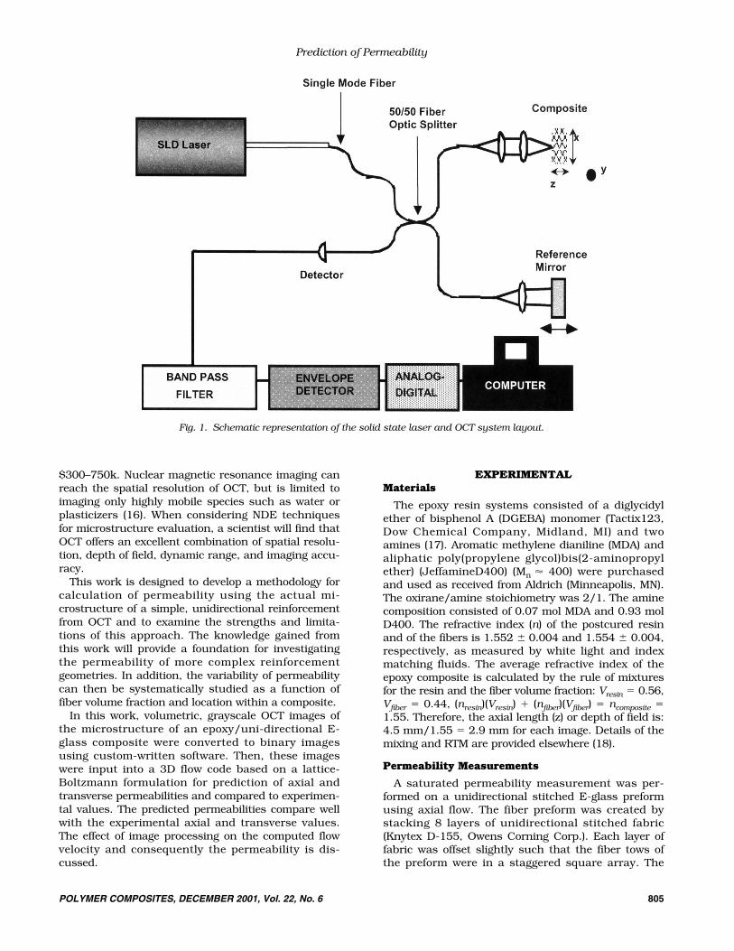
reference light beam, for an incident light beam topenetrate and backscatter within the sample. Thistemporal delay is probed using a fiber-optic interfer-ometer and a broadband laser light source. The fiber-optic interferometer consists of single-mode opticalfiber coupled with a 50/50 fiber-optic splitter that il-luminates both the sample and a linearly translatingreference mirror. Light reflected from the referencemirror recombines with light backscattered and re-flected from the sample at the 50/50 splitter to createa temporal interference pattern, which is measuredwith a photodiode detector. The resulting interferencepatterns are present only when the optical path differ-ence of the reference arm matches that of the samplearm to within the coherence length of the source. Theaxial, or z, spatial resolution that can be obtainedwith OCT is determined by the coherence length, orinverse spectral width, of the source and is typically(10 to 20) �m (Fig. 1). The source is typically a super-luminescent diode laser, with a maximum axial reso-lution of 7 �m. The transverse, or x, spatial resolutionof OCT is determined by the focal spot size on thesample which is typically (10 to 40) �m. The ultimatelimitation on the depth of penetration within the sam-ple is the attenuation of light caused by scattering.Three-dimensional images of the sample are obtainedby rastering the sample in x between successive OCTmeasurements along the y-axis.

OCT as a nondestructive evaluation (NDE) tool com-pares very favorably to more established compositeNDE techniques. Both transducer and laser based ul-trasonics have been used for NDE of polymer compos-ites. Their practical resolution is on the order of 1 mmwith tens of mm penetration depth (12, 13). A majordrawback to ultrasonics is that the depth of a featuremust be determined by model studies, whereas, it isdetermined straightforwardly using OCT. However, ul-trasonic testing can evaluate carbon fiber composites,which absorb too much light to be examined by opti-cal techniques. Both OCT and ultrasonics suffer fromcontrast degradation and shadowing through thesample thickness. Two X-ray based techniques havebeen widely used. X-ray radiography is the more es-tablished technique, with a spatial resolution of hun-dreds of micrometers and tens of millimeters in pene-tration depth (14). The main drawback in performingX-ray radiography is that it results in a two-dimen-sional representation of three dimensional features. Amethod more recently applied to composites, X-raycomputed tomography (CT), has a resolution similarto OCT and penetration similar to X-ray radiography.Features that do not have a separation, like somecracks, may not be detected. The accuracy of the X-ray attenuation, and thereby the feature intensity andposition, is a complex function of many variables, andadditional constraints complicate image interpretation(15). However, a great deal of work on image analysisof X-ray tomographic images has resulted in well-established commercial software packages, but thecost of X-ray CT systems is still very high, about

Joy P. Dunkers, et al.

804 POLYMER COMPOSITES, DECEMBER 2001, Vol. 22, No. 6

$300–750k. Nuclear magnetic resonance imaging canreach the spatial resolution of OCT, but is limited toimaging only highly mobile species such as water orplasticizers (16). When considering NDE techniquesfor microstructure evaluation, a scientist will find thatOCT offers an excellent combination of spatial resolu-tion, depth of field, dynamic range, and imaging accu-racy.

This work is designed to develop a methodology forcalculation of permeability using the actual mi-crostructure of a simple, unidirectional reinforcementfrom OCT and to examine the strengths and limita-tions of this approach. The knowledge gained fromthis work will provide a foundation for investigatingthe permeability of more complex reinforcementgeometries. In addition, the variability of permeabilitycan then be systematically studied as a function offiber volume fraction and location within a composite.

In this work, volumetric, grayscale OCT images ofthe microstructure of an epoxy/uni-directional E-glass composite were converted to binary imagesusing custom-written software. Then, these imageswere input into a 3D flow code based on a lattice-Boltzmann formulation for prediction of axial andtransverse permeabilities and compared to experimen-tal values. The predicted permeabilities compare wellwith the experimental axial and transverse values.The effect of image processing on the computed flowvelocity and consequently the permeability is dis-cussed.

EXPERIMENTALMaterials

The epoxy resin systems consisted of a diglycidylether of bisphenol A (DGEBA) monomer (Tactix123,Dow Chemical Company, Midland, MI) and twoamines (17). Aromatic methylene dianiline (MDA) andaliphatic poly(propylene glycol)bis(2-aminopropylether) (JeffamineD400) (Mn � 400) were purchasedand used as received from Aldrich (Minneapolis, MN).The oxirane/amine stoichiometry was 2/1. The aminecomposition consisted of 0.07 mol MDA and 0.93 molD400. The refractive index (n) of the postcured resinand of the fibers is 1.552 � 0.004 and 1.554 � 0.004,respectively, as measured by white light and indexmatching fluids. The average refractive index of theepoxy composite is calculated by the rule of mixturesfor the resin and the fiber volume fraction: Vresin � 0.56,Vfiber � 0.44, (nresin)(Vresin) � (nfiber)(Vfiber) � ncomposite �1.55. Therefore, the axial length (z) or depth of field is:4.5 mm/1.55 � 2.9 mm for each image. Details of themixing and RTM are provided elsewhere (18).

Permeability Measurements

A saturated permeability measurement was per-formed on a unidirectional stitched E-glass preformusing axial flow. The fiber preform was created bystacking 8 layers of unidirectional stitched fabric(Knytex D-155, Owens Corning Corp.). Each layer offabric was offset slightly such that the fiber tows ofthe preform were in a staggered square array. The

Prediction of Permeability


Fig. 1. Schematic representation of the solid state laser and OCT system layout.

fabric was oriented with the flow direction parallel tothe fiber tow direction. The overall dimensions of thepreform were 15 cm wide (x), 15 cm long (y), and 1.3cm thick (z). Several measurements were conducted ina narrow range of fiber volume fractions to obtain areliable average value as well as error estimates. Themodel fluid used was a corn syrup solution. The vis-cosity of the corn syrup solution was measured usinga controlled stress rheometer (Bohlin, Visco88). Theviscosity was 0.110 Pa•s at 23°C. The flow behaviorwas Newtonian over the shear rates examined.

The corn syrup solution was injected into the moldunder constant pressure conditions. The resin was al-lowed to flow through the fiber preform until it be-came fully saturated. After saturation occurred, thevolumetric flow rate and mold inlet pressures weremeasured at several control valve positions. A seriesof six measurements of the volumetric flow rates andinlet pressures were taken at each valve position overa range of inlet pressures from 0 kPa to 30 kPa. Thevolumetric flow rate was cycled through this pressurerange to ensure that there were no changes in thepreform characteristics as a result of the flow. The rel-ative standard uncertainty in the average volumetricflow rate at each control valve position was less than2% of the average volumetric flow reading. The stan-dard uncertainty in the inlet pressure readings was0.1 kPa. The permeability was determined from theslope of the linear regression of the volumetric flowrate versus inlet pressure data. The R2 value for thelinear regression was 0.99. The resulting axial perme-abilities are shown in Table 1 for similar fiber volumefractions. The average saturated permeability for flowalong the fiber tows is 5.3 10–6 cm2 with an uncer-tainty of 2.6 10–6 cm2.

A radial flow experiment was performed for calcula-tion of the transverse permeabilities. The flow anisot-ropy was found by measuring the ellipticity of the radialflow front (Table 1). As expected, the radial flow experi-ment also indicated that the major axis of the in-planepermeability tensor lies along the tow direction. Thetransverse permeability was calculated by multiplyingthe square of the ellipticity by the axial permeabilityobtained from the saturated flow experiments.

OCT Instrumentation

The OCT imaging system used in this study is sche-matically shown in Fig. 1. A commercial superlumines-cent (SLD) light source (AFC Technologies Inc., Hull,Quebec, Canada) is used for the studies reported here.

The source operates at 1.3 �m with an output powerof up to 15 mW and a spectral bandwidth of 40 nm.The laser light is coupled into a single-mode fiber-opticMichelson interferometer and is delivered to both thereference mirror and the sample. The reference mirroris mounted on a rotating galvanometer, which is drivenwith a sawtooth voltage waveform. Transverse scan-ning is performed using a computer controlled motor-ized stage to translate the sample.

The interferometric signal is electronically filteredwith a bandpass centered on the fringe or heterodynefrequency. The filtered fringe waveform is then de-modulated, digitized and stored on a computer. Thehigh dynamic range of this system allows back-reflec-tions as weak as a few femtowatts of power to be de-tected. Images are displayed by mapping the loga-rithm of the signal strength to a grayscale look-uptable. The acquisition time for each image is approxi-mately 1 min. The axial (z) measurement range is de-termined by the distance the reference mirror moves(4.5 mm) normalized by the refractive index (n) of thesample: 4.5 mm/n. The probe beam is focused to a 30�m diameter spot at a depth of approximately (750 to1000) �m below the surface of the sample.

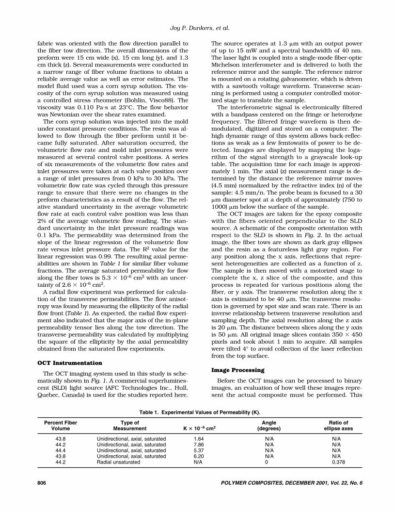
The OCT images are taken for the epoxy compositewith the fibers oriented perpendicular to the SLDsource. A schematic of the composite orientation withrespect to the SLD is shown in Fig. 2. In the actualimage, the fiber tows are shown as dark gray ellipsesand the resin as a featureless light gray region. Forany position along the x axis, reflections that repre-sent heterogeneities are collected as a function of z.The sample is then moved with a motorized stage tocomplete the x, z slice of the composite, and thisprocess is repeated for various positions along thefiber, or y axis. The transverse resolution along the xaxis is estimated to be 40 �m. The transverse resolu-tion is governed by spot size and scan rate. There is aninverse relationship between transverse resolution andsampling depth. The axial resolution along the z axisis 20 �m. The distance between slices along the y axisis 50 �m. All original image slices contain 350 450pixels and took about 1 min to acquire. All sampleswere tilted 4° to avoid collection of the laser reflectionfrom the top surface.

Image Processing

Before the OCT images can be processed to binaryimages, an evaluation of how well these images repre-sent the actual composite must be performed. This



Table 1. Experimental Values of Permeability (K).

Percent Fiber Type of Angle Ratio of Volume Measurement K � 10–6 cm2 (degrees) ellipse axes

43.8 Unidirectional, axial, saturated 1.64 N/A N/A44.2 Unidirectional, axial, saturated 7.86 N/A N/A44.4 Unidirectional, axial, saturated 5.37 N/A N/A43.8 Unidirectional, axial, saturated 6.20 N/A N/A44.2 Radial unsaturated N/A 0 0.378

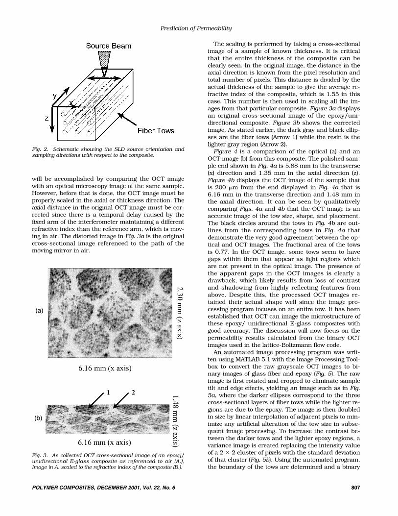
will be accomplished by comparing the OCT imagewith an optical microscopy image of the same sample.However, before that is done, the OCT image must beproperly scaled in the axial or thickness direction. Theaxial distance in the original OCT image must be cor-rected since there is a temporal delay caused by thefixed arm of the interferometer maintaining a differentrefractive index than the reference arm, which is mov-ing in air. The distorted image in Fig. 3a is the originalcross-sectional image referenced to the path of themoving mirror in air.

The scaling is performed by taking a cross-sectionalimage of a sample of known thickness. It is criticalthat the entire thickness of the composite can beclearly seen. In the original image, the distance in theaxial direction is known from the pixel resolution andtotal number of pixels. This distance is divided by theactual thickness of the sample to give the average re-fractive index of the composite, which is 1.55 in thiscase. This number is then used in scaling all the im-ages from that particular composite. Figure 3a displaysan original cross-sectional image of the epoxy/uni-directional composite. Figure 3b shows the correctedimage. As stated earlier, the dark gray and black ellip-ses are the fiber tows (Arrow 1) while the resin is thelighter gray region (Arrow 2).

Figure 4 is a comparison of the optical (a) and anOCT image (b) from this composite. The polished sam-ple end shown in Fig. 4a is 5.88 mm in the transverse(x) direction and 1.35 mm in the axial direction (z).Figure 4b displays the OCT image of the sample thatis 200 �m from the end displayed in Fig. 4a that is6.16 mm in the transverse direction and 1.48 mm inthe axial direction. It can be seen by qualitativelycomparing Figs. 4a and 4b that the OCT image is anaccurate image of the tow size, shape, and placement.The black circles around the tows in Fig. 4b are out-lines from the corresponding tows in Fig. 4a thatdemonstrate the very good agreement between the op-tical and OCT images. The fractional area of the towsis 0.77. In the OCT image, some tows seem to havegaps within them that appear as light regions whichare not present in the optical image. The presence ofthe apparent gaps in the OCT images is clearly adrawback, which likely results from loss of contrastand shadowing from highly reflecting features fromabove. Despite this, the processed OCT images re-tained their actual shape well since the image pro-cessing program focuses on an entire tow. It has beenestablished that OCT can image the microstructure ofthese epoxy/ unidirectional E-glass composites withgood accuracy. The discussion will now focus on thepermeability results calculated from the binary OCTimages used in the lattice-Boltzmann flow code.

An automated image processing program was writ-ten using MATLAB 5.1 with the Image Processing Tool-box to convert the raw grayscale OCT images to bi-nary images of glass fiber and epoxy (Fig. 5). The rawimage is first rotated and cropped to eliminate sampletilt and edge effects, yielding an image such as in Fig.5a, where the darker ellipses correspond to the threecross-sectional layers of fiber tows while the lighter re-gions are due to the epoxy. The image is then doubledin size by linear interpolation of adjacent pixels to min-imize any artificial alteration of the tow size in subse-quent image processing. To increase the contrast be-tween the darker tows and the lighter epoxy regions, avariance image is created replacing the intensity valueof a 2 2 cluster of pixels with the standard deviationof that cluster (Fig. 5b). Using the automated program,the boundary of the tows are determined and a binary



Fig. 2. Schematic showing the SLD source orientation andsampling directions with respect to the composite.

(a)

(b)

Fig. 3. As collected OCT cross-sectional image of an epoxy/unidirectional E-glass composite as referenced to air (A.),Image in A. scaled to the refractive index of the composite (B.).



Fig. 4. Optical microscopy photograph of the sample end (A.), OCT image of the composite in A., 200 �m from the sample end (B.).

Fig. 5. Pre-processed OCT image(A.), variance image (B.), binaryimage (C.), filled final image (D.).

image (Fig. 5c) is formed. In the next two steps, spuri-ous “on” pixels within the image and vertical lines cor-responding to detector saturation are eliminated. Theimage is the scaled to the proper aspect ratio and a fill-ing operation is applied to better define the tows as isseen in Fig. 5d. The resulting binary image is thenused as input for the permeability calculation. An ad-ditional operation may be performed to smooth therough boundaries of the tows.

Numerical Simulation

Governing Equations

Modeling the microscale flow in fibrous porous mediais complicated by the existence of an open regionaround the tows, and a porous media inside the tows.Following previous studies, (3–6, 8) the Stokes equa-tion, given by

(2)

is used to model flow in the open regions, and theBrinkman equation, given by

(3)

is used to model flow in the porous regions, where K=1is the permeability of the porous tows. In both re-gions, the continuity equation,

(4)

is used to model conservation of mass.

Lattice-Boltzmann Method

Solutions to the governing equations above are ob-tained using a lattice-Boltzmann method described indetail elsewhere (5, 6). In short, the method involvesthe solution of the discrete Boltzmann equation forthe particle velocity distribution function n(x, t),where traditional fluid flow quantities such as densityand velocity are obtained through the moment sums

(5)

(6)

where �(x, t ) and u (x, t ) are the macroscopic fluid den-sity and velocity, m is the mass of fluid, v are compo-nents of the discrete velocity space, and N is the num-ber of velocities comprising the velocity space. Theparticle distribution function n(x, t ) is governed bythe discrete Boltzmann equation given by

(7)

where �(x, t ) is the collision operator which couplesthe set of velocity states v. Most LB formulations em-ploy the linear “BGK” form (19–23) of the collision op-erator in which the distribution function is expandedabout its equilibrium value

(8)

where neq (x, t ) is called the equilibrium distribution

function and is a relaxation time for collisions con-trolling the rate of approach to equilibrium. The formof the equilibrium distribution function depends onthe particular lattice model chosen. The three-dimen-sional, “d3q15” model (20), which resides on a cubiclattice, is used here (d3 indicates the model is three-dimensional, q15 refers to the number of componentsin the velocity space). For this model, the equilibriumdistribution function is given by

(9)

(10)

(11)

where

(12)

v � ce, c is the lattice speed, and e are the unitvectors along each of the lattice directions in the dis-crete velocity space, and F is a body force. To recoverthe physics associated with the Brinkman equation,the body force

(13)

is introduced, where s(x) is a function equal to 1 inporous media and 0 in open regions. This approachhas been validated in previous work.

Permeability Computation

Permeability for different flow directions was com-puted by imposing a constant pressure along oppositefaces of the lattice in the desired direction and inte-grating the system of equations above to steady-state.The boundary conditions are imposed using theextrapolation scheme of Chen et al. (24), and the im-plementation is described in detail in Spaid and Phe-lan (6). The boundaries of the flow domain are as-sumed to be periodic along the faces normal to theflow direction. In all of the simulations, the resolutionwas 299 73 in the x-z plane (as indicated in Fig. 2).The depth of resolution in the y-direction is indicatedby the number of images in Table 2. Estimates for theintra-tow permeability values were obtained from pre-vious work (3). The steady-state velocity field at theinlet was integrated over the surface to obtain the flowrate, Q, and this was used in the formula

F ��s 1x 2 �K �

�1 # u

ueq � u � # F

�

n15 �29

� a1 �32

1ueq # ueq 2

c 2b

a1 � 31e

# ueq 2c

�92

1e

# ueq 22c 2

�32

1ueq # ueq 2

c 2b , � 7, 14

n �172

�

a1 � 31e

# ueq 2c

�92

1e

# ueq 22c 2

�32

1ueq # ueq 2

c 2b , � 1,6

n �19

�

�1x, t 2 � �n1x, t 2 � n

eq 1x, t 2

n1x � v,t � 1 2 � n1x, t 2 � �1x, t 2

u �m

�1x, t 2 aN

�1v n1x, t 2

� � maN

�1n1x, t 2

§ # u � 0

§�P � � �§2�u� � �K1�1 # �u�

§P � �§2u



(14)

to obtain the effective permeability, Keff, for the de-sired direction.

RESULTS AND DISCUSSION

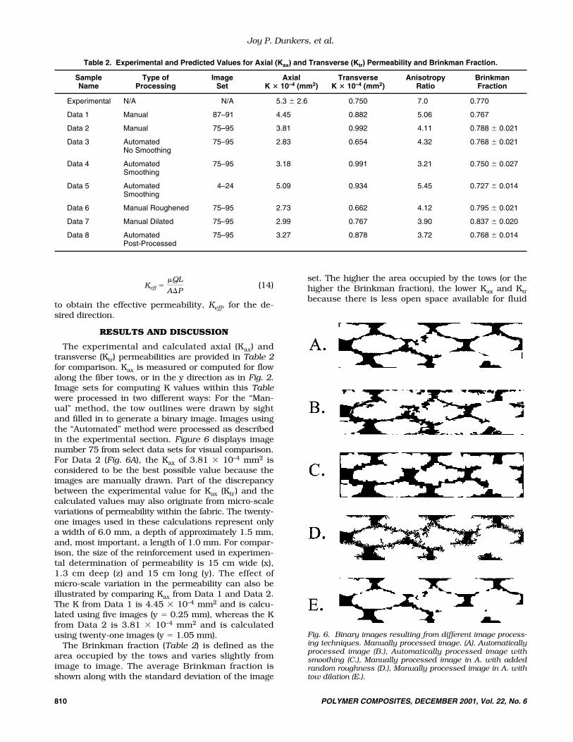
The experimental and calculated axial (Kax) andtransverse (Ktr) permeabilities are provided in Table 2for comparison. Kax is measured or computed for flowalong the fiber tows, or in the y direction as in Fig. 2.Image sets for computing K values within this Tablewere processed in two different ways: For the “Man-ual” method, the tow outlines were drawn by sightand filled in to generate a binary image. Images usingthe “Automated” method were processed as describedin the experimental section. Figure 6 displays imagenumber 75 from select data sets for visual comparison.For Data 2 (Fig. 6A), the Kax of 3.81 10–4 mm2 isconsidered to be the best possible value because theimages are manually drawn. Part of the discrepancybetween the experimental value for Kax (Ktr) and thecalculated values may also originate from micro-scalevariations of permeability within the fabric. The twenty-one images used in these calculations represent onlya width of 6.0 mm, a depth of approximately 1.5 mm,and, most important, a length of 1.0 mm. For compar-ison, the size of the reinforcement used in experimen-tal determination of permeability is 15 cm wide (x),1.3 cm deep (z) and 15 cm long (y). The effect ofmicro-scale variation in the permeability can also beillustrated by comparing Kax from Data 1 and Data 2.The K from Data 1 is 4.45 10–4 mm2 and is calcu-lated using five images (y � 0.25 mm), whereas the Kfrom Data 2 is 3.81 10–4 mm2 and is calculatedusing twenty-one images (y � 1.05 mm).

The Brinkman fraction (Table 2) is defined as thearea occupied by the tows and varies slightly fromimage to image. The average Brinkman fraction isshown along with the standard deviation of the image

set. The higher the area occupied by the tows (or thehigher the Brinkman fraction), the lower Kax and Ktrbecause there is less open space available for fluid

Keff ��QL

A¢P



Table 2. Experimental and Predicted Values for Axial (Kax) and Transverse (Ktr) Permeability and Brinkman Fraction.

Sample Type of Image Axial Transverse Anisotropy BrinkmanName Processing Set K � 10–4 (mm2) K � 10–4 (mm2) Ratio Fraction

Experimental N/A N/A 5.3 � 2.6 0.750 7.0 0.770

Data 1 Manual 87–91 4.45 0.882 5.06 0.767

Data 2 Manual 75–95 3.81 0.992 4.11 0.788 � 0.021

Data 3 Automated 75–95 2.83 0.654 4.32 0.768 � 0.021No Smoothing

Data 4 Automated 75–95 3.18 0.991 3.21 0.750 � 0.027Smoothing

Data 5 Automated 4–24 5.09 0.934 5.45 0.727 � 0.014Smoothing

Data 6 Manual Roughened 75–95 2.73 0.662 4.12 0.795 � 0.021

Data 7 Manual Dilated 75–95 2.99 0.767 3.90 0.837 � 0.020

Data 8 Automated 75–95 3.27 0.878 3.72 0.768 � 0.014Post-Processed

Fig. 6. Binary images resulting from different image process-ing techniques. Manually processed image. (A). Automaticallyprocessed image (B.), Automatically processed image withsmoothing (C.), Manually processed image in A. with addedrandom roughness (D.), Manually processed image in A. withtow dilation (E.).

flow. If the Brinkman fractions are considered, thenthe Kax for Data 3 (Fig. 6B) should be higher than forData 2 (Fig. 6A) since the Brinkman fraction for Data3 is slightly lower than for Data 2. For the automati-cally processed images in Data 3, the Kax is in factlower than for Data 2. In short, rough tow boundariesare very effective in suppressing fluid velocity andthus artificially decrease permeability. More explana-tion is provided later in the text. From these results, itis evident that improving the smoothness of the towboundaries is an important next step.

To improve the smoothness of the tow boundaries, asmoothing operation in the form of a binary openingand closing was performed on the automatically proc-essed data. Data 4 from Table 2 shows the resultingpermeability and Brinkman fraction of the smootheddata. A corresponding image is shown in Fig. 6C.Upon smoothing, the permeability increases. However,the resulting Brinkman fraction is substantially lowerthan for the manually processed images. Thus, thisparticular smoothing operation is considered to be anunsatisfactory procedure for the image data.

However, comparing the permeability between Data4 and Data 5 is valid since the same amount ofsmoothing was applied to each image set. The largedifference in permeabilities between Data 4 and Data5 again illustrates the micro-scale variation of perme-ability within the reinforcement. Again, both imagesets represent a 1.05-mm-long section of sample.Image set 75–95 is 2.55 mm farther down the samplethan image set 4–24. Image set 4–24 has three imagesthat contain crossing threads while image set 75–95has 15 images with crossing threads. These crossingthreads are processed into the image as connectionsbetween the layers of tows. For the permeability cal-culation, they are assigned the same intrinsic perme-ability as the glass tows and also act to suppress thefluid flow. It has been shown experimentally thatcrossing threads have a large influence on decreasingthe permeability and that removal of the crossingthreads led to as much as a factor of six increase inthe experimentally determined permeability when thesame fiber volume fractions and packing geometrieswere compared (25).

The effect of tow roughness on permeability is illus-trated when the permeability results from Data 6 (Fig.6D) and Data 7 (Fig. 6E ) are compared. The imagesfrom Data 6 (Fig. 6D ) are originally from Data 2 (Fig.6A), the manually processed images. However, a smallamount of random roughness was introduced in Data

6 while retaining nominally the same Brinkman frac-tion, leading to an increase in tow surface area. ForData 7, the images in Data 2 were dilated to increasethe Brinkman fraction, but the roughness was not al-tered. When the axial K from Data 7 is compared toData 6, the result is initially unexpected. A relativeincrease of roughly 4% of the Brinkman fraction inData 7 should lead to a decrease in Kax over Data 6,but the result is the opposite. The Kax of Data 7 ishigher than Data 6. This comparison between the per-meabilities from Data 6 and Data 7 means that sur-face roughness is comparable to or more influentialthan Brinkman fraction in influencing permeabilitywhen changes of similar magnitude are compared.

The measure of tow roughness used in this work isthe tow surface area. A relative surface area was cal-culated for each image in the data set by applying anedge detection algorithm in MATLAB that retainedonly the edge pixels as “on” pixels. Then, the numberof these “on” pixels was computed and normalized tothe total number of pixels in the image. This numberis called the relative surface area. Table 3 shows therelative surface areas computed for Data sets 2, 3, 6,and 7. The surface area to which the other data iscompared is from the manually processed images ofData 2 and is 6.2 � 0.4, where 0.4 is the standard de-viation. Note that for the automatically processed im-ages in Data 3, the relative surface area is 2.1%higher than for Data 2. Of greater interest is the sur-face area of the roughened manually processed tows(Data 6) which is 2.4% higher than for Data 2. For thedilated tows in Data 7, the surface area is about 0.7%lower than for Data 2 because the dilation increasedthe connectivity between the tows. From these results,knowledge of the Brinkman fraction and tow surfaceareas points to both as important contributors to per-meability. The relative magnitude of their contribu-tions is not yet known. These results also highlightthe importance of processing the images as close tothe actual structure as possible.

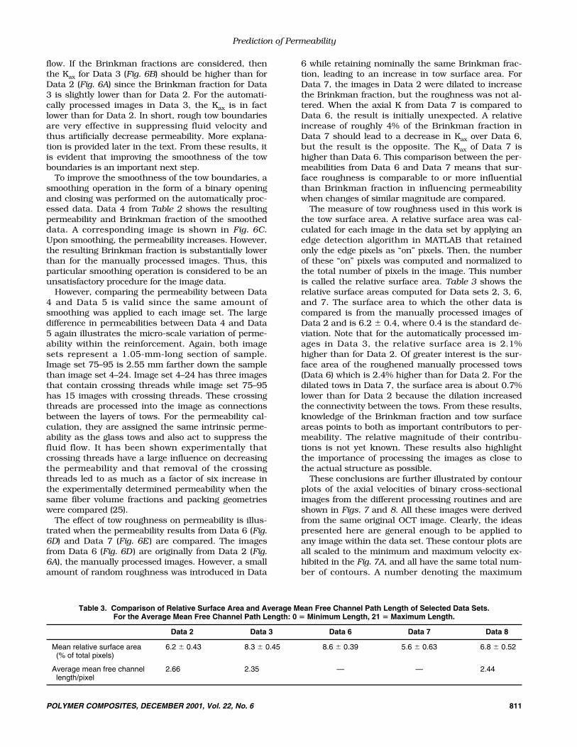
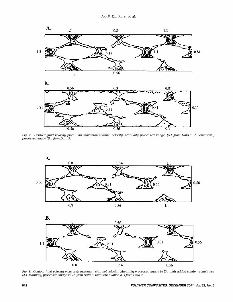
These conclusions are further illustrated by contourplots of the axial velocities of binary cross-sectionalimages from the different processing routines and areshown in Figs. 7 and 8. All these images were derivedfrom the same original OCT image. Clearly, the ideaspresented here are general enough to be applied toany image within the data set. These contour plots areall scaled to the minimum and maximum velocity ex-hibited in the Fig. 7A, and all have the same total num-ber of contours. A number denoting the maximum



Table 3. Comparison of Relative Surface Area and Average Mean Free Channel Path Length of Selected Data Sets.For the Average Mean Free Channel Path Length: 0 � Minimum Length, 21 � Maximum Length.

Data 2 Data 3 Data 6 Data 7 Data 8

Mean relative surface area 6.2 � 0.43 8.3 � 0.45 8.6 � 0.39 5.6 � 0.63 6.8 � 0.52(% of total pixels)

Average mean free channel 2.66 2.35 — — 2.44length/pixel



Fig. 7. Contour fluid velocity plots with maximum channel velocity. Manually processed image. (A.), from Data 2. Automaticallyprocessed image (B.), from Data 3.

Fig. 8. Contour fluid velocity plots with maximum channel velocity. Manually processed image in 7A. with added random roughness(A.). Manually processed image in 7A from Data 6, with tow dilation (B.) from Data 7.

velocity in the channel is provided near the channel.The velocity is the smallest at tow boundary and ex-hibits a maximum in the center of the channel be-tween the tows.

The images in Fig. 7 illustrate the influence on thetow boundary roughness on permeability. If Fig. 7B iscompared to Fig. 7A, it is clear that the maximum ve-locities in the center of the channels is always lessthan or equal to that in the manually processed im-ages in Fig. 7A. This is despite the fact that theBrinkman area of the automatically processed tows isabout 3% smaller than for the manually processedtows. If Fig. 7B is examined, one can see that overall,the velocity contours are smaller and more irregularlyshaped than in Fig. 7A. Also, the velocity contourstake on the shape of the nearest tow, and this shapeinfluences velocity to the center of the channel whereincreased resistance to flow occurs from the roughboundary.

More compelling examples are provided in Figs. 8Aand 8B. Random roughness was added to Fig. 8A thataccounted for only a 0.7% increase in the Brinkmanfraction relative to the manually processed images(Fig. 7A). However, a 30% decrease in permeability re-sulted from the small scale roughness present in Fig.8A that caused irregularities in the shape of the veloc-ity contours and suppression of flow. The decrease inpermeability when the tows are dilated as in Fig. 8Bwhen compared to 7A is caused by simply a decreasein channel radius available for flow. The velocity maxi-mum decreases while shape of the velocity contours isretained.

In order to preserve the Brinkman fraction whileminimizing tow roughness, the automatically proc-essed images were subjected further post-processingroutine, which eliminates small “peninsulas” emanat-ing from the surface of the tows and then fills in theremaining small “inlets” on the tow surface. A repre-sentative post-processed image is shown in Fig. 9Aalong with the corresponding manually (Fig. 9B ) andautomatically (Fig. 9C ) processed images. Figure 9A isderived from Fig. 9C through the post-processing rou-tine, but obtains much of the smoothness and Brink-man fraction as Fig. 9B. The relative surface area ofthe resulting data, Data 8, is markedly closer to thesurface area of the manually processed image (Data 2)as shown in Table 3.

The previous discussion has shown the influence ofthe free channel radius. However, the free channelpath length [i.e. the number of image slices a fluid ele-ment can travel along one pixel in the y-direction (par-allel to the tow direction) before hitting an obstruc-tion] also influences permeability. This concept issimilar to the capillary tortuosity that was discussedin previous work that described the reinforcement interms of fractals (7). The exact distribution of freepath lengths can be calculated using a simple com-puter program. For each pixel, a mean free path length(average of all free path segments encountered movingin the y-direction along one pixel) is calculated. Since

21 images slices were used in the calculation, a valueof zero indicates no free path length (i.e. a tow is pre-sent) while 21 indicates an unobstructed path. Theaverages of all the mean free path length per pixel val-ues are shown in Table 3. These values do give an in-dication of the amount of obstruction presented bythe reconstructed tows, but do not necessarily give anindication of free channel radii or connectedness ofthe free channels in the xz-plane. However, the valuesof average mean free path length per pixel do correlatemonotonically with the calculated permeabilities. Theaverage mean free path length of the post-processedimages (Data 8) is an intermediate value between theautomatically (Data 3) and the manually (Data 2)processed images. The higher value for Data 8 relativeto Data 3 despite the similar Brinkman fractions is aresult of the smoother tow boundaries. The fluid trav-els a less tortuous path near the tows for images inData 8, which, in conjunction with a slightly largerfree channel radius, enables a higher fluid velocitymaximum than for Data 3. The resulting axial andtransverse permeabilities are higher than for the origi-nal processing program, and are in excellent agree-ment with the range of expected values from our ex-periment. In addition, this post-processing routine iscompletely automated, allowing for the tows to be re-constructed more rapidly than the manual techniquewithout the influence of human bias.



Fig. 9. Binary images resulting from different image process-ing techniques. Post-processed image (A.), Manually processedimage (B.), Automatically processed image (C.).

CONCLUSIONS

The microstructure of a unidirectional glass-rein-forced composite was accurately and rapidly obtainedusing optical coherence tomography. OCT imageswere processed and input into a microscale flowmodel for permeability prediction. It was found thatthe Brinkman fraction, the tow surface area, and theaverage mean free channel path generated by theimage processing have an important influence on theaccuracy of the permeability calculations when com-pared to the expected values. By optimizing these ef-fects during image processing, excellent agreementbetween the calculated and the experimental axialand transverse permeabilities was obtained. However,only a small portion of the composite was sampled.The variability of the permeability throughout thecomposite still needs to be evaluated on many sam-ples. Only by doing this can a true comparison be-tween the experimental and predicted results be per-formed.

A number of enhancements to this methodology willbe implemented for future work on more complex rein-forcements. First, images of the entire cross-section ofthe composite are already being obtained with im-proved OCT instrumentation. Second, a more robustimage processing method based on image gradients tosmooth and recognize features will be implemented forthe more complex, three-dimensional reinforcements.

ACKNOWLEDGMENT

This work was supported in part by a grant fromthe U.S. Department of Commerce, contract70NANB6H0092. We gratefully acknowledge technicalcontributions of Dr. Juergen Herrmann, Dr. WolfgangDrexler, and Mr. Rohit Prasankumar.

REFERENCES

1. R. Parnas and A. Salem, Polymer Composites, 14, 383(1993).

2. H. Friedman, R. Johnson, B. Miller, D. Salem, and R.Parnas, Polymer Composites, 18, 663 (1997).

3. S. Ranganathan, G. Wise, F. Phelan Jr., R. Parnas, andS. Advani, Proc. ACCE94, 309 (1994).

4. F. Phelan Jr. and G. Wise, Composites: Part A, 27A(1),25 (1996).

5. M. Spaid and F. Phelan Jr., Phys. Fluids, 9(9), 2468(1997).

6. M. Spaid and F. Phelan Jr., Composites: Part A, 29, 749(1998).

7. R. Pitchumani and B. Ramakrishnan, Int. J. Heat MassTransfer, 42(12), 2219 (1999).

8. S. Ranganathan, R. Easterling, S. Advani, and F. PhelanJr., Polymers & Polymer Composites, 6(2), 63 (1998).

9. D. Huang, E. Swanson, C. Lin, J. Schuman, W. Stin-son, W. Chang, M. Hee, T. Flotte, K. Gregory, C. Puli-afito, and J. Fujimoto, Science, 254, 1178 (1991).

10. J. Fujimoto, M. Brezinski, G. Tearney, S. Boppart, B.Bouma, M. Hee, J. Southern, and E. Swanson, NatureMedicine, 1, 970 (1995).

11. M. Bashkansky, M. Duncan, M. Kahn, D. Lewis, and J.Reintjes, Opt. Lett., 22, 61 (1997).

12. S. Wooh and I. Daniel, Materials Evaluation, 48(5),1206 (1994).

13. R. Dewhurst, R. He, and Q. Shan, Materials Evaluation,51(8), 935 (1993).

14. A. Highsmith and S. Keshav, J. Comp. Tech. Res., 19(1),10 (1997).

15. R. Bossi and G. Georgeson, Materials Evaluation, 53(10),1198 (1995).

16. P. Jezzard, C. Wiggins, T. Carpenter, L. Hall, J. Barnes,P. Jackson, and N. Clayden, J. Mat. Sci., 27(23), 6365(1992).

17. Identification of a commercial product is made only tofacilitate experimental reproducibility and to adequatelydescribe experimental procedure. In no case does itimply endorsement by NIST or imply that it is necessar-ily the best product for the experimental procedure.

18. J. Dunkers, R. Parnas, C. Zimba, R. Peterson, K. Flynn,J. Fujimoto, and B. Bouma, Composites, Part A, 39,139 (1999).

19. S. Chen, H. Chen, D. Martinez, and W. H. Matthaeus,Phys Rev. Lett., 67, 3776 (1991).

20. Y. H. Qian, D. d’Humieres, and P. Lallemand, Europhys.Lett., 17, 479 (1992).

21. Y. H. Qian and S. A. Orzag, Europhys. Lett., 21, 255(1993).

22. P. L. Phatnager, E. P. Gross, and M. Krook, Phys. Rev.,94, 511 (1954).

23. S. Hou, “Lattice Boltzmann Method for Incompressible,Viscous Flow,” PhD dissertation, Department of Mechani-cal Engineering, Kansas State University, Manhattan,Kansas (1995).

24. S. Chen, S. Martinez, and R. Mei, Phys. Fluids, 8, 460(1996).

25. F. Phelan, Jr., Y. Leung, and R. Parnas, J. Therm. Comp.Mat., 7, 208 (1994).



Documents

The Prediction of Permeability for an Epoxy/E-Glass