Embed Size (px)
Citation preview

THE PREDICTION OF THE INTERACTION BETVVEEN
SHIPBOARD ANTENNAS AND THEIR ENVIRONMENT

DECLARAri iONI
I declare IIH~l: this dissertation is my own, unaided work, It is being submitted for the
Degree of Master of Science in Engineering at the University of the Witwatersrand,!
J()hanJ1esbu~i~'It has notbeen submitted before for any degree or examination in any
other Ullive~·~ily.

ABSTRACT
This dissertation discusses the interaction between shipboard antennas and their
cnvironmem.
The emphasis is on the Use of the Method of Moments to calculate the currents on
the structure of the ship. These currents are induced by the antennas mounted on the
structure of the ::;hip.
The parameters (such as grid spacing and wire radius) to use in creating a wire grid
model of the ship is investigated and recommended values. given,cj
A sample ship is ll!ltllyzed and the results obtained compared with meas~relnents
done in an unechelc chamber.
o 0
,~.
u

s
ACKNOWLEDGEMENTS
The author would like to acknowledge the help and suggestions of his supervisor,
Prof Hanrahhan. The author would also like to acknowledge the help of Dr B. A.
Austin under whose supervision this dissertation was started.
The author is indebted to his employers, the CSIR, for support of his research and
permission to publish th~swork.
Dct,dicate4 to Celeste.
i)
C \) o
f)o
c,
<J
(I
~I

Table of Contents
f)ECLARA l'10N i
A.BSTRACT ii
ACKNOWLEDGEMENTS ................................... ~ 0· t ., ' , , "11"'. '. iii
LIST OF SYMBOLS ••••••••.••• , ••••.••.••••.•••••.•••• , ..................•••••.•••••• ' ••••.••.•••• , •••••••.•••• 'j!
NOMENCLATURE ............................. t' ~.;, '0 * •.••. ~ Ii t" t, .. xi
1 INTRODUCTION ., ,. 11.11'hc need for prediction .. 11.2 Preview of work 41.3 Ea~lkr work in prediction , 51.4 Predlction methods used " 9
1.4.1 Model measurement ".,,, 91.4.2 Mcthqd of Moments (MM) , 10J .4.3 Geometrical Theory of Diffraction (GTD) , ,....... 11t~414.1·lybridmethods <r-.tn H..H "'h.\\ .•9•.•,. n.t-.. t~,,,,,.,,,, •• ,,., 12
j \
i)
2TUB 1\U~TI'IODOF MOMENTS i ••............... : 142~'iIntl"()uuctiQn "".HHH.h" "H .•• .:H.IJt.;;h •• Uh".:.ft.\.~}UHH ••• t: ,,...tlt. ••• iio "t'.~ ; 141:'2..2 Moment Methods' n.".t,H_~ ••••• '.I.f-.H h •• ~•••• l,." .. f l •• H , HOl'!:.hlr ". i.42!13,Prograrn' NEC2. r-. u" •• ~ " -.." •• .,1i:.H ••• ~•••• 4t ••• <i H:."' ~•• 1i •• ~-;' H1.. 172'"'41.)r()g~alllFliWIR'Eil ~1H .• .:; " H ... i>Il,'H'1i. .... <;,HhW,H"'<tH -H ,. .. 4 .. '... H?IiH~".~h .. ir ... 252.5 Proglnm ESP,.-: ••..,.•.-~HR ,"U.,_t ..HIr •• "it-,._,..- •••• " •• ,.-,. .... ~ ... H.,.,.'.HitI •• H.'.~.-••U ·h.tlll!U, •.. ,272.6 ycrifying the Method"ofMoments with dipoles ,.» ';., 3:12:7 Modelling Surface Structures , " ,,362....8 Discnsslon ....-"''''.'...-H •• ,·' ....... ''H ... Hl .. ~.t.H lj •• H.t H H,. ••• H._ (). HH':.ltH H. 4'6
o
'·3J{I~t.Jf,/1"S{' 'H••• ~.. ~7H..h II~,.. -"., O -(i'Hh ,,_t.li-'l~ 4 ••• ,fh H." •• :•• ' .. H ••• ~ H 4,'73.11Jltrpdtt'ction ;Ht1UU -n"' <I •• ~ I."",•• ~,..~.'f.-f.t fH •• ~.,.h ••• "' ••• "' ,·~\).lL•• 473.2 g_cl)l11ctry of ship, ': 473.3 First nlodel.·(lvlodel A) _H.""nh~ "t ..~.t~H••••• h.HH~_.U .••• i<~.HlI••• H t •• ~.. U.,~'.~..; 473.4 Second model, (Model B) " 'w H .. "' : .. " :. 513..5 ,1hi(f11nodeL (Model C) Hu••HU,(~; 'i iljt' <Ii •••• u l\.-u ".n,•• 573.Xi L1isttlssi-on Hn t.u.,.H 'jo.~, H lI••• ~H.IoH._ ••• f •.• tU~~ •• 1O••• " "" iI." .. i u'l'u 63
~.'
o4.1 Surnnrary .:t.. ~•., .,H •• "hn H "' HU •• I!"t.lf .. n ·:'••• h._H-' U.H' H':U<I:"' ,,.. ..
4-",2Further work. H •• n~<t .. ~ , :: 1"' ••• f .H~ ,.i ~~~-n U .~,"1"" tHHft!oh :':\1. , t ...
666~67
o
~, . ;~
_51{EI:I~I~13NCI!S.-..t~ l\ n- H.~ ..~t", •• " •. ,.~.tI' ¥ '.. iol'h •• ;.) ..'~ ;-., ;," •• H'oI"".-.; ".*. 7Q,"II _ .... . _ ..' \~',"" . v . .' __ .~'
I\~PENDIX A. INTnORAL EQUATIONS " ',." 14 e
A.I Maxwell's Equntions '.' \L, ;,}.•,,~~ , ~. 74A.2 TIm potential Integro-Differentlal Equation '17A.3 Pm:klington's IntegI'M Eqmrti<1/1 .. " 79'0
iv
AA The Reaction Integral Equation (RIB). ;,; 80
APPENDIX B. MEASUREMENTS ON SHIP MODEL 84
APPENDIX C. TABULATED RESULTS OF DIPOLE STUDY 88
t\'('PENDIX D. WIRE RADIUS OF A SQUARE GRID 90
APPENDIX E. WIRE RADIUS OF A TRIANGULAR GR!D 92
c- II
v"
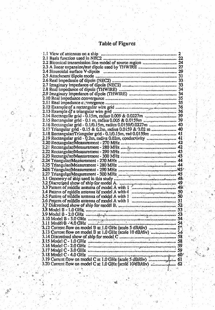
Table of Figures
1.1 View of antennas on a ship 22.1 Basis function used in NEC2 222.2 Biconicnl transmission line model of source region 242.3 A linear expansion/test dipole used by THWIRE 272.4 Sinusoidal surface V -dipole " ' " 292.5 Attachmesrtllpole mode 3]2.6 Real impedance of dipole (NEC2) 332.7 Imaginary impedance of dipole (NEC2) ." 332.8 Real impedance of dipole (THWIRE) , 342.9 Imaginary Impedance of dipole (THWIRE) 342.10 Real impedanceconvergence " 352.11 Real impedance C::1vcrgence 352.12 Exampleqf a rectangular wire grid ~~ , 362.13 Example q! a triangular wire grid ., : 362.14 Rcctangt0trr grid - 0.15m, radius 0.009 & 0.0227m , , 392.15 Rectangular grid - 0.1 111, radius 0.005 & 0.0159m " 392.16 Rectangular grid - 0.1/0.15111,radius 0.0159/0.0227m 402.17 Triangular grid - 0.15 & 0.2m, radius 0.0159 & ').02 m 402.18 R.cctungularffriangular grid- 0.1/0J5m, radO.0159m " 417.19 Rectangular grid - Q2t11, radifls 0.02111,conductivity ." " , 412.20 Rect.urgular/Measurement - 270 MHz ." m ,. 422..21 Rccmngq!at/Measurell1cnt - 280 MH?; \y" 422.22 Rectangulnr/Measurement - 290 MHz '..· ~I 432.23 Rec!an~ti.larlMeasurell1ent" 300 MHz " "." 432.24 Triangular/Measurement" 270 MHz H ". 442.25 TriangularJ,MeasureB1cnt :..280 MHz " ''' ".;~ 441~i26Triangular/Measurement ~.29()MHz , ,,>rtl5"2.27 Triunglll~r/Mea,~t1rement - 300 MHz ~ " , ''' 453.1 G!!ometry of ship used in this sWdy ~ :; " , ;, ~ 48,3.2piscret~$cd show of ship for model A. T , ; 493.3 Pattern of middle. antenna of model A wish 1 c; 49,3.4 Pattern of middle antenna of model A witt]"! : \,.. 503.5 Pattern of llliddle antenna of Il1ddel A with 1 : ~ 503.6 Pattcni of mt!1dle antenna of mod cd A with 1 ",.. 5.13.7 Di~~rctiscd. show of ship for model B, ; 523:8 MndclB ,.1.0 GHz, " ~ ~ H 53:t9 Model B ~2.0 OHz _;;.".;~ "' " "'. 53:t10 Model I3 - 3.0 GH.z ~.:.; "." , ~' 54:~.11.Modc.l\B .24.0 GHz '~''';':~H H.'HUH .. hH H 'H H .. j' H •• hHj;''.H ••• i 54:~.12Current flow on-model B at J.O GHz (scale 5 dB/div) : ;~~3.13 Current flow 011 model Bat 1.0 GHz (scale 10 d13/div) ~63.14 Discretised show of ship for model,C ,. " " 58:[15' iv10del C ,;,...1.0 Gl·lz .., ·.i. ••• u ' .H' HH"'h •• ,. '~ "h H ,58:U6 Model C - 2.fJGHz ~w ') 59,~J.17MO(I~lC ..3.,0GHz '.!\ '~h •• fH.oi, ..HH •• H._ "'.·,.. ~•••• HH~ :' ... h, ~;,.i.Uu""'-."'!I"':'U'!tH" 59~L18 Mmfcl C ~4.0 GHz " H "."' .., H.: ~f 1( ' 601/:U9 Current flow on model C at to GHz (scale 5 dB/dlV) 'H" )!~,~..613.20 Current flow on model Cat 1.0 GHz (sca!8' 1O,ltlB/div) ',1,4.. 62
Ii
IfG
vi
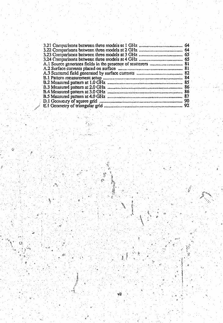
3.21 Comparisons between three models at 1 GHz 643.22 Comparisons between three models at 2 GHz 643.23 Comparisons between three models at 3 GHz 653.24 Comparisons between three models at 4 GHz 65A.l Source generates fields ill the presence of scatterers 81A.2 Surface currents placed on surface ., 81A.3 Scattered field generated by surface currents 82B.! Pattern measurement setup 84B.2 Measured pattern at 1.0GHz "..... 85B.3 Measured pattern at 2.0 GHz 8613.4Measured pattern at 3.0 GHz 86B.5 Measured pattern at 4.0 Gl-lz " .. 87D.l Geometry of square grid ., 90B.1 Geometry of triangular grid 92
vii
o
If,
Table of Tables
2:1 Results obtained of dipole using NEC2 " 882.2 Results obtained of dipole using THWIRE. .. 89
o
GJr1'
:j
viii

LIST OF SYMBOLS
E Electric field
f frequency
I I Magnetic. field
1 Current
J Current density
k Propagation constant
r disl:tncg from origin
time
V Voltage
x Iii's; t()o~Ulll1tein rcctungulUr coordinate system
,.,
y second ccordinate in rectangular c90r~in'at~ system
l)l1\tdcoordinate in rectangular coordinate'system(
(_';'·'.·,f
i\vaveh~ngth
(ll wavenumber w defined as,21rf
:\~\;
-,tl angle between z axis and vector tnl/spherical coordinate system\\
D
ix

~) angle bctweenx axis and projected vector in x-y plane in spherical coordinate
o degree
p vector ill x-y plane in cylindrical coordinate system
mathematical del operator
i,\
:i\,
'-,
(jo
)1~)
C-'
x

N01\1ENCLATURE
dB
DF
EFIE
EMf>
ESP
o[[z
GTD
fiF
MFIE
Ivf} Iz
MMQ -
NEC2 ;;llr
decibel
Direction Finding
Electrical Field Integral Equation
Electromagnetic Pulse
Computer program with surface formulation
Gigahertz
Geometrical Theory of D:;ffraction
IUgh Frequency (2 - 30 MHz)
Magnetic Field fntegral Equation
.Mcgahertz
Method of Moment
Computer program develol)ed at Lawrence Liver~ot'i: N~ltional
LaboratoriesII.
RADI1AZ Radirfdon Hazard"
HF
(l
,l
xiI>
G
'1'( iWIRE Computer program developed at Ohio State University
UIIF Ultra High Frequency (300 - 3000 MHz)
VHF Very High Frequency (30 ~300MHz)
VSWR Voltage Standing Wave Ratio
xii e
o

1 INTRODUCTION
1.1 The need for prediction
The various clements of a ship's superstructure such as the masts, funnels and
different decks constitute a complex scattering and reradiating environment for any
antenna. Any antenna located within such an environment will possess radiating
characteristics considerably different from the same characteristics under free space
conditions.
Degradation from the ideal is most apparent with wide beamwldth antennas,
especially omnidirectional antennas such as those l'cquired for certain forms of
communications and Direction Finding (DF) systems. Departure from' the ideal free
space behavior leads to'C11'01'S ill DF systems andto less d~an optimum performance"
for communication systems.
.~... (\. ....Unfortunately, thc~e antennas cannot tie sited, so that their rRd,~t.\tionpatterns ate
Ul1ilffccteUby any neighboting superstructUre or any other atlten~a system, This is. . . - . - - \\
because, no ttntenlld can exist in isolation on a ship's cro vdeddecks t\nc:tmasts. Figure" " " ", 16
L l: shovls a typicaH'iew of antennas on ~.:ship. ,At best one must try ;it number of
<.Jifferent antenna locations to find the IOy,~tion where the unwanted effects elf the
superstructure on the antenna are tpit1imized. "d
'In this thesis I will use the tt~rmradiation pattern even for a r-cceiving antenna because\\" ..... \~
of reciprocity, The reciprocitYltheotel'11(1)p49:lstates thatlhel'udtation and receiving\) '._ - - _. ;- - I:l - 1\,I
paucrqs of Itll antenna are e\l{aci~~1,hesame. 0
IIIIIi'I
..,~I:.')" o
(i
""1 .":}....... '7
I(1"),
0;-
j Q
t")D
o
"
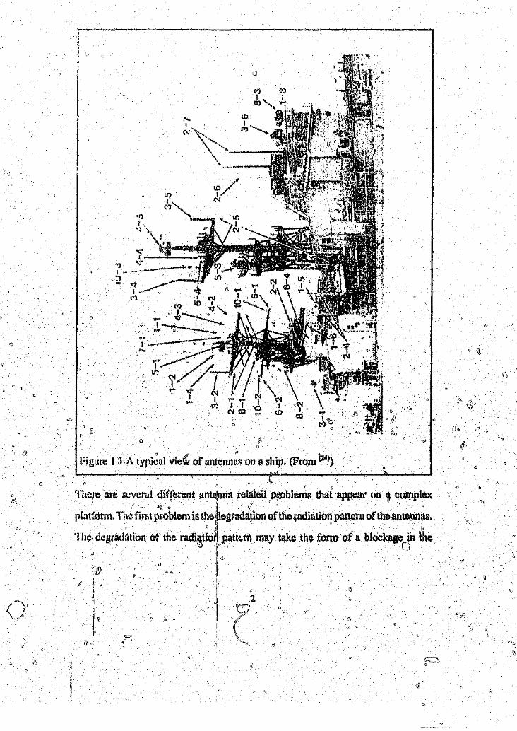
Figure J rl.Atypical vie.\\. of antenl1tis on a ship. (From (t4»~--------------~--'-------4r----------~--~----~u
There are several different ant~~na rehited ~)~()blemsthat appear on ~ complex~ 0 ~
platform. The. fi rst problem is the )~egrnda~iollof the ~ndiation pattern of the antennas,(.) :1 " ,"" ,"" _', ," _(,
The" degradation &1the l'adi~tiori~"pattern may take the fonn of a blOckagedn tbei' ~
Ii11I'
I!I'r~li"ili'
\1
(I
('l
('II

pattern where there may be loss of signal (and thus comrnunication) in a specific
direction. It may also be in the form of multi path where a signal may be received by
more than one path (some direct rays and othersreflected or diffracted rays). The
different rays wl11then add in and out of phase and so created a distorted pattern.
If'structures in the near field ofthe antenna are excited such that currents comparable
to the size of the currents on the antennas begin to flow, the actual currents on the
antenna will be Changed. This will not only cause problems in the radiation pattern
of the antenna, but also in the impedance (and thus in the VSWR) ()f the antenna.
This means that less power is being transmitted, and that some equipment will not, ,
work _(Jropcrlyor may even be damaged hyJhe reflected power.ij • .~
o
D
Htrcause of ihc close Pl'OXullity of the antennas on the platfonn, the Ievelof receptiQ,n " o~ . 0
'0
of an untlcsircd signul by an antenna 1Sipctease~.LAn example is a communicatic,mI_' <'
\ 'l~a;~smis:.i()nbeing received on an navigation ant6nnu. \fhe level of this undesired(,
" . _.. ". (i,; ~ . I)
signul rnus! be controlled as far as possible for acceptable system performance to be(J. ._ -.,; . o
obtained. This 18 usua~JY done by mouut.tngJmtennus connected to ,higli, pow~~)
tmnsmiUcl'sas far as possiblcl awftcY fromuntcnnas cqnuecteq. to selt$itiv~c~IVf~.~."II " .'
, \: ~ 0 0
, A problem [hat is. getting mc)re .attention lately is the problemofradiatiotl hazards.~) - -_ . .' .. ' '" -_.~. . '.' (..."
(R)\~HAZ). TI&isis where i'tteJeveI ofelemric energy is so largethat it posse~s' aC._ ... . . '1)
hazard tOlR't',\OI1!1cL(for example a worker In frolltof a hl'gh power ra<:latantenua), ',\ () .;.
or ,to fuel and explosives. For effective control pf RA.qHAZ the energy levels at\\ " . .'.... '.: . b
different plm;(!s on the ship must' be known .•If areas witl{higb ru" p&wer levels are 0 G
l,i !i
ificntified, control measures such as the establishment of rcstri~.ted areas arourtdtransmit all£eruUis can be taken.
t! i,;}:1
o
G
o
3
()

The single most important reason why a method to predict the performance of an
untcnna in the presence of the;ship is needed, is because of the high cost of moving
antenna installations on ships, A further problem is the measurement of the radiated
field from an antenna installed on a ship.
By'using tnctimds to predict thc, performance 'llf the antennas in the presence of the
ship, it is possible to try a fair number of different antenna locatlons to find an
0I)timmn location. Such an option is much cheaper than to install antennas using
trail and e;1tor,:,tcchniqucs.
Prc<,lictiOlHl1CthcRis can)Ilso be used as diagnostic Mols to try and.solve problems
,in existing installatiollj;hy ghoing the amdystmore insight into the physics ofradiation()(\ .... ::
cbnracrerlsiies.
/)
1.2 Preview of workc
() .
The ne>« lntmgraph O.S) gives a summary of earlier work in precljction. Paragraph,~ ,',.. .. . G
D 0measurement, the M,¢dlOd of Moments, Geometrical Theory of Diffraction and
'.,(.1, n \\. c,,\ ~j (~ h.) C
hybrid mctlu)ds. " ... ;";l
The Method of Moment~ i~ tbe supj~ct 0'chapter 2: Aft~r an introduction,·theo \). ~\ .' ~.. ,~
·M()Il1Cnt Ml,:.t!fod';lsdescribed. The.thre~ computer prf>grams used in this study are;: . . ,Ii. .
then described. A study is described toverify the Met1 rod Of Moments using dipoles."
The parameters nece~sary to model'a s~Hd surface J["",~owire gtR{are deter~ined.,'. .'. . .... ; ....,_,.,~/
"fh(t~llUptcr is ended with a short discussio~ of the results.o
:-:1
4
o
a(!

\1
Chaptcr J discusses the results obtairied during the modelling ora ship. Three models
of increasing complexity are described and the results shown. At the end of the
chapter a discussion of the results is given.'
~hapter 4 shows the conclusions drawn from the results obtained. After a summary
of the results, further possible extensions ate discussed.
The references used are shown in chapter 5.
Appendix A shows the details of some integral equations.
Appendix B shows the details of the measurements made on the ship model.
Appendix C ';!rows the result of the dipole study in tabular form,(I
Ap,1endix D and E show respectively the derivation of the necessary wire radius to''"
u~eQf()rsquare and triangular meshes.
o
°Moore ;md PizcrP) give ~xery good introductioiLlntolhe Method or Moments. The(;>'. ' \:~~,~. ;;::- ,;; \\
tlJost lmp()rti~nt.integral· equu,tions are described. Some computer c~s 'that ~he
authors have used are, descrlbed, Gev~rill practical applications of the MethQ<:l.of
Moments nrc also discussed in this book:One of tlte important aspects discussed is ao
the Jlse of wire grid modelling for the modelling of {loUdsurfaces. Although the work" (;) . '\ .\" a . .(t' 1\ . (J
'>': ( ' ,- , II
In the'll'book is baseq on soatterlng problems. it g~ve a very good starting point for/fJ l! -;,; - 0 ," 'j,>
the antenna on ship problem.
5
\~,o
Butler and Wilton (:1) show several numerical techniques to solve Pocklington '8 and
I lallen 's equations for thin-wire scatterers. The basis functions cons'dered include
the piecewise sinusoidal, piecewise linear and trigonometric functions. Various types
of testing schemes such as collocation and Galerkir» are used. The authors come to
the conclusion that to obtain acceptable convergence rates, discontinuities in the
current approximation and its derivatives must be suppressed. Another useful
technique is to circumvent the effect of such discontinuities by making the equ,~tion
insensitive to them. Tris may be done by uslng averaging techniques such :1$ usinga Galerkln tcchniq\lc." ,"
Pearson and Butler (4) discuss the inadequacies of the collocation solutions to
PocklingtolHype '"models of thin-wire structures. The basis functions Uiilder
discussion are Ih~~ieccwise sinusoidal functions. It is shown that with point matching~..-1...t",...... ,> ;:; ,(I, I
this type hfhii )~ictioll ha51i{tI~ utility. 0 \)
-. ">, _.-ic
Wdnlloud (5) introduces the principle of using a wire grid to rpodel It continuous
surface. He. uses an unifrofrn current density con each segment with point matchingb::>
<It the center of the segments. Scattering from the surfaces is modelled. He was ableo
c
to solve problems with a maximum of 100 unknowns, that is, up to "one square.
wilvel~l1gih ill size.V\ ctl~cularplate ofr~~ius 0,15 Awas ~odelled with 3 t~61igonal'" 'I 1 ~rings (2.0 sides each)" at ~dii of 0,05,6,10 and 0,15, A. The eente'! ofJhe ~late was~ ,o \\ 0)
left open ..The wire radlus tva~taken as 0.005 A.. A square plate~w~thsize that changed" 6'_ 0 0 , .. "C \)
(I
lipm OJ.w 1,1 A" was modelled with 8.wir.es in each direction. The wire diameter, . . . .. . . (l .. ,) (J
was tiAk~nto he ~ii(hof the length of the plate. o()\\.
I) v
oi\ \7'0
6o n

('"almon and Smith (6) use wire grid modelling to calculate the current on a surface.
The fields close to the surface are then determined. The wire grid used by the authors
is in the order of 0, 1 A. in size. The authors found that with care the near field can be
calculated us close as one grid spacing away from the surface.
Jambrinu andAnL.\es (7) show predicted and measured results of a.twin fan antenna
and monopole centered on top of a conducting box over an infini.te groundplane, The
size of the boxes, used was"of the same order of those of the antennas considered.
According to the article the distances between parallel wires of the mesh we~~ kept
[0 less than a quarter wavelength. Fromthe figure supplied in the article it looks as
if more parallel wires were used. The radiiwere chosen so that the tot~1wire surface
was twice ,thill of the origina! surface, Reasonable results were obtained by them. "
'o Kubina and Larose (8) did a study where they modelled a dipole near a mast built ofo ~ c .
tubular segmcnts.: Predigtions were done Using both wires with jhe Method of(i{J,. ':rE
.Moments (NEC2) and four fiat plates with the deonletri.£~l Theory of Diffraction(J,f~ ':
feTD). Very slrnilar results were~obtainedwith b()~liiieth()ds. A maximum segment»: .",~"..
n " ... ', '., . . .' . ,.(.\1:':'\'·
length of 0.2 It.was used itt the Method ~~M6mentstudy.
IJ
~"." ""
c .r/,~\iY'. . '. ,_
" W()q~l1jt!lji~~ld.Slemp (9) discu,~~S:ijhysical modellim;; of shipb8rne antennas.' The. . ~
fuctorq th~ ~postBe used in eleC(:omagnetic SC8.er modelling of a:ntP~llas are shown.
The lnost/ll1ff0rtant changes thi'nmst be made are the change of physical sizes.l ' '"'frc,ljucl1v!Y and the conductance of all material,$,f -. "" .;.
l"\ Ne~tJ;l~cull (11)) give a techniqt1e for realistic:modelllng ofarbitmry structures with
\;_ if - -, If (J
'\pVIx~onu:l patches. ,Aft.er a short introductiQ.l1,details of the treatmentof touching\c'. \:J 'Q
=
o
7

.,
plates with overlapping patches are given. Three examples of scattering solutions
are given namely a rocket, the Concorde aircraft and the Boeing 747 aircraft. It should
be noted that the frequency used is'low, such that the rocketis 2,4 Along, theConcorde
1,8 Aand WeBoeing 747 1,3 A.
Rockway and Du Brul (11) state in their overview of shipboard antenna system
predictions the following two basic facts. Firstly, no rigorous algorithms can be
developed for selecting antenna locations until all the factors influencing the
desirability of an antenna site have beer;:identified and their influence on the system
associated. with the candidate antenna determined. Furthermore " factors
i'nfluencing antenna site desirability cannot be determined until all al'ltcnnas are
}(>cU1cd.The two basic facts are incompatible and can only be solved simultaneously
llsirlg some iterative technique. T~rY furt~:ermade a comparison between the use of
numerical modelling and physical modelling. The conclusion is reached that the two
Iechniques nrc 4'()1l1pleni'cntnry'DThedirect cost tor the ~umerlca1 modelling relative
to physical' modclling'was great,er because of the cost of co'mputer ti41o, While theI; ~";.
ma'Jl)OWcr cost was cOOl:liderably lower.o o
Llidwig (2~) t,:~xa~1illedthe mO#elling of sllPfa.ces \Yid~a ,Wire grid. He recognized thato D
the results obtained using a wire grid tflodel of~ .solid surface are s~n&itive to thec
-I):;' q,.. .' . /' _ " "" '"" iJ
wire diam(t!J~d·Hcthen exan~illed the pr,\?bIemofwire gddm9dellingusing an infinite~, , , ' ,':;', , ' ' ' .', "',',, ,". ',_. c' '" _'0, "._, , ' ",,', ' ,, __' .. ,,'
long cylinder. Exact results for both th~~true l1foblem and the wire grid model werea - -.;~ ,,' L , ' " • r!
used, Tbis isolated the effects of wire gddm9delllng fr~>mother eff~cts ofthe Method".,\
of MO,Plcnls.ll~ comes "tothe conctuslon t*i1t the best itf::Clilracyis obtained when the,,' . ;;'.v
f; 'Q
0
1)
0(,/
8(I
,\
wire diameter satlfies the 'same surface area' rule of thumb. The effect of too thick
wires is just as bad as too thin wires. He also shows that the boundary value match
between wires is not a reliable check on the validity of far-field results.
1.4 Prediction methods used
Various methods to predict the performance of antennas on ships are available, The.
followbg four methods and variations of them are the best known.
1.4.1 Mod(!1measurement
Model measurement as applied to antennas on ships is l! technique by whiph the
C) radiating characteristics of physically large structures (such as an antenn £,\. 'on a~ship)n ],
fire determitlcd by doing antenna measurements on suitably dimensiqned sca!e
models.
The seRle nonnp' Iy ~ls¢dis 1!48J and this means that a frequency of 30MH~is ~~,a.ledli. ... ,_ \_\ I_ ,_ -', _ n
Ina fr~ttlwncy ()$'l 44~ MHil\B~C~l,Use of the high frequencies enCQUritel¢, tb~ 8
highdst frl1qll~rncy'ba41dmodelled is usually the ..tIF band, although some ~lodelling ", :, il 1~ . ? ,', . _ - 'c' - ':' Ii - - 8 c; Ytuker(p1it(tc in the UHF b!~md(l2~.'
fJ
. The mitin dism.1yillltal?l.ll of titIs technique Is the high ihithdcostof building/a accu~te". " -', - v --~~ " /J" _, ',' - "j!' ,)
model olfth~ shill: It is also very difficult to model any nOtl~conduct~'lgpart such as(;0
parl~made nldieleetrlcor mugnetie,matenals (eg. composit~ materialssucq as carbon
t1bre and fibrcglass), Tb be able to model such matetials n "very large range of- - ,,',' - -', --,' /)
!I
()
\1
9

0.
o
muteriuls with different dielectric and magnetic constants must be available. It I&:
believed that more composite materials will be used in future in the ship building
process,
Another major problem is the tirnescales needed to complete such a model. The
model needs to include ail the detail of the original ship and the surface finish needs
to be ifif a comparable standard (taxing the scale factor into account) to the real ship.j\
n is flil'i"-:-:-~""}lOre quite di.f!1cu1tand expensive to make any major changes to the"-<
ship's structure after initial construction of the model,>.'\,.:_/,~.,.,-
An advantage of model measurements is the fact )h~tonce a model has been built
uPt~llarge number bfmeasurernents can be done in a fairly short time. This is possible,.
because of automated n;casl.1rement techniques. 'fa do the scale measurements a
properlydcvcI()ped antenna measurement facility must be available. Such a facility~>~); /.:
needs to be able to q,pe.rate'9"1ef'u, large frequency range. Mea§t1rements muet alsofh . .' . '. ~~j'_~_.. .~f , :,)
be done on n large groundplane;", >:> . -,' .-/;
1.4.2 Method of Moments (MM)o
Elcctmmag. nellli radiation (Dr sc~{~6rin~)problems can a~ys be represented by anc ,;/"
integralequntiol1. This eCluatlon car{pnly be solved rigorously in a rew special Cases.Q ' ''''' "'.' ' ,", , \,', n ,-,
l"e M.Jh"~"(M~~n~ illVOlves thoMueli~n p( tb¢ associated ;nt"~hl equationOt~ a system of linear algebraiB '/equafion~. The unknowns of this system are
coefficients in,s()me'~ppropriale expansion of the current. By solvinglhe result1n~.'r.~
10

nuurix equation, the currents on the structure can be computed. From the currents
secondary parameters such as far fields, near fields, impedances and coupling can
be obtained.
The'number of simultaneous equations to be solved is directly related to the total
size of the structure and the frequency. This means that for larger structures more
equations are needed, while more equations follow at higher frequencies. This leads
to the main disadvantage of thi~ technique, namely that the amount of equations
needed to be solvcd becomes larger than can be solved in a reasonable time and at
a reasonaijJc cost,
1.4:3Geometrical Theory of Di'ffracfion (GTD)
The Geometrical Theory of Diffraction is used where the wavelength uSl:";dis much.... . .. .~"sl)}aller than the structure under investigation. It is then, possible to describe the
electromagnetic wave interaction as optical rays, bouncingbetween scattering points ..-/' ,"
<rhe basic scattering mechanlams at these points are dlffractionand reflection. The
"Iuteraetion between a source and an observeJllis detetmtn~a by adding contributit.msL 1\ 'ii' ,> U
1'1'001 all the po~§ipleray paths and mechanisms' between the two. 'I 0
The-~~'ipleneeded for i!\ GTO solution is.not determined by the size,of the structure
hut by tIle Humber of possible rays that must be traced. This means that large structuresu
can be analysed quite easily if the number of ray paths for the structure is smaJl.this
,is usually true fQI'large bodies that have no concave surfaces.GTDdoes not requireo "
'';1''';
a large memory, Them"lain limi!ution of the OTD is that for all diffraction coefficientsI)
11o

to be valid. all reflection/diffraction and source points as well as all geometrical
dlmenslons must be in the order of at least one wavelength apart, This may be relaxed
to a quarter wavelength for engineering purposes.
1.4.4 Hybrid methods
Because of the limitations of the Method of Moments and the OTD several types of
hybrid methods were developed. Two such methods are described briefly below.
The GTD/MM hybrid method is one such method. The Method of Moments is used
to de~ermine diffraction coefficients which are used in the OTD solution, This method
is mostly used in the analysis of antennas where the diffraction coefficients of certain
cs' structures a§~not known. An example of this method is found in the work done at
Ohio State Un~vcrsityol1 theradjationpatterns of aperture matched horns (l:l>, ~/
" .'. r. .' .. ,(~"(Gi.. . • ' . . .' it:' . H'IThe MMIOTD hybrid method is another class of hybrid methods, In this r,J "~">~:,~,i";
" " .,'. ," .. "'. '''_''>r''~''<' .
Method of Moments solution is set up for.·the antennas and tbeir it~tt.ledi~C1
neighborhood. Ina true MM/OTD hybrid metHOd the resulting interactiQn-.;~atriX is':1. - '. \'. . . . __ . ._.... ... - ,;
then modified by adding the contributiotfs of reflections andlor diffractions from
fur-off (bu~ still ill the near ..field) structures. This. procedur~:~esults in"~i reduced .
mafrix (thus less storage needed)oan~ in most cases in reduced comput~Hpn time., ,.',1f' - ,?
o In a simple MM/GTD method the. currents 'ot' just the anteri'na and its immediate
surr()undh~ will be computed assuming that the rest of the sl:rUctur~doos"nrJtexist.
TheQurrents ofthls area 'Still then he used to obtai,n tlie far fields of the ~tenna in~~ . ,!
the presence of the whole structure, 'SIlL's'method makes the assumption dlat the\~
12,
!I
o
currerits on the antenna are n.,t affected by the structure. An ext:tmple of this method
is when ii small wire antenna such as a ultra high frequency (TJHF) yagi is mounted
on a large structure such as a building.
\l
1,1
o
,:" f)
n13
13

2 THg METHOD OF MOMENTS
2.1 Introduction
The Method of Moments is a method whereby the radiation or scattering structure
considered is divided in smaller sections (usually called segments or modes). The
electromagnetic interactions between these sections are then computed as an
impedance matrix. A voltage vector is set up according to the excitation field. Thus
the problem is reduced to all equivalent set of simultaneous equations. This set of
.sinlUltal~e()USequations is then solved to obtain the current on the structure. FJqm
thccurrents secondary parameters such ashnpedance.coupllng andra. iatlonpatterns
can tbe derived.
For the purpose of this discussion we limit ourselves to radiation and scatteringfrom,~~ . " 1;
t~()nd\lcti!1gstructures.
2.2 Moment Methods(I
l~mm Maxyv'clI'5 equations we can derive a linear integral equation. Appendi.x A
shows l~p'e~nmple of such atVl9Jegral equ~tiot1./" ..','<",;:'.'."
Following the procedure itt (2} t1e fQJlowing is a introductlon t9 the Moment Method.()
Consider t1)~')nhomogeneous'equation (it
(2.1)
o
o
14

where
too is ~ linear operator,
F a known function and
<1> a function to be determined.
III the case of electromagnetic problems LQ) is normally an integral or
intcgl'O·(Hffcrential operator, c.l> is the distribution of electrical current and r the
impressed field or the applied voltage. <I> and r are both functions of the spatial<C
coordin~Hes and of the frequency.
Tile current distribution m can now be expressed in terms of known functions using,-'
undetermined parameters, for example, as a linear combination of a finite number
of ballis or expansion functions <!Jj in the domain of L(J)thus
(2.2)
"The constants rl.j, 'which'are finite in number, must now he determined. By(,i
") !:
SUbSljtuting (2.2) into (2,.1) we get,'"
II (2~3)(/
'Yhich for a linear op~ratbr leads to"I
o ,;1
(2.4)
15o
o
o
o
o
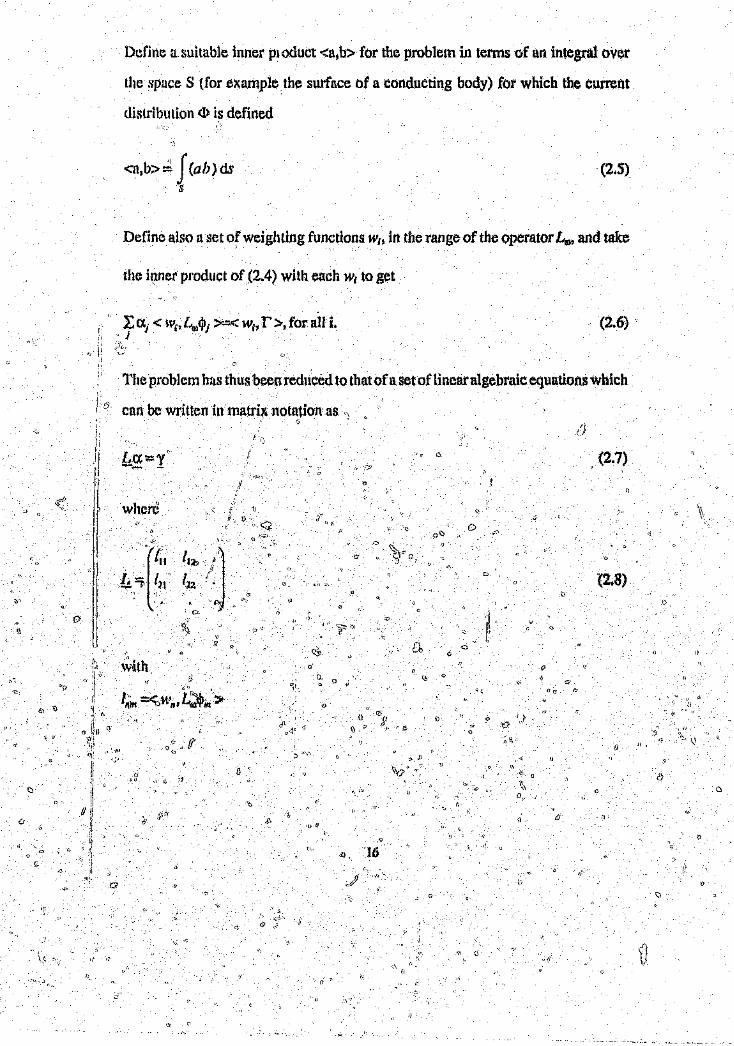
Define a suitable inner product <a.b> for the problem in terms of an integral over
the space S (for example the surface of a conducting body) for which the current
disuibution <P is defined
<a,b>:=; f (ah)dss
(2.5)
Define also a set of weighting functions Wi! in the range of the operator LOll and take
the iuner product of (2.4) with each Wi to get
~ cx)< w"LOl<Jlj >::::<Wi' r>, for all 1.J
(2.6)
The problem has thus been reduced to that of a set of linear algebraic equations which
can be written inmatrix notation as
.. (2.7)
whereIJ
(2.8)a
with\;;
" oII
«
(/
\'c;o

(2.9)
(2.10)
with
"Equution (Z.7) CUllbe solved using any of the stftndaclJ~~~"\~1:cc'-'~~r~~Ja9,\~fizati()n,
of the It,mutrix, / r-, ?;;~:
t: ",(~ r""lh "\":-u,'t~,'. I~'~'"
The aspuracYJUld efficiency,of the method dep(:'ll~i~v1:1~i'gescale t)nlhe choice Qf\":''?',.:~
", ,'. I{, " ..,' , c:.)·,the basis fun,9tiuns o/i~~l~Weigl\::,)g functiqns Wj' N(')r~H\ny the basis and weighting
..' " . .
fUtlctiOl'l is bhosell sUe'h that each is 0I11ymon~zero0',/,;;;1'a regio" small compared to'_, " . " '". '" ' .I' >~~:::...., !
., the'.wdvel,e!J~th.Hy uSing many sl,lch functions over tfi~\,~:.sY, a body of arbitrary~" ,',',.
.shape can be constructed ind~p¢ncIently of the specific basis functions.
""'''''', !),','.} .,1
_',' \,_ \
2.3 Program NEC2.''" \\
()
\, '-", . \\ "
Th~ NEC2 pr~grriU1 (M.15,l6) is a conl~uter code used to solve for th'~currents on win
" wires: or closed surfaces, In this st1dY only the thin wire modelllng capability ofo .. ... ,) "
~!)
NEC2 is used. anc no "detaHof the surface mooeHing is given.
uQ
o
o 11
\\n,
o

The integral equation used by NEC2 is an electric-field integral equation (EFlE)
which follows from an integral representation for the electric field of a volume current
distribution 7 :
E(i) =:4~~i7(i') •G(i;i')dV'
where
G(r,r') =: (k2j +M)g(r,f')
using Ihe time convemion (!V(l){). j is the identity dyad c;e;e +"lY +U).
(2.11)
If we consider a perfectly conducting body with th~ current distribution lim,fted to
the surface of the body, equatiq~(2.11) he~omest,,)
t) e .
E(r)= -jl1 rJl.rr'): O(r"r')dA'43tk Js 'J
(2.12)
\ with J$ r,}le surface current pe,lJsit~'.The observatipn point r is restricted to be,offthef 0 ()
.1:\ ". '
surface S so that r if:. ;::' or else g(r, r')J:!ecomes unbounded: '"
If.; approaches S as a limit, eq~latioii 2.12 becomes, Ii
:;c r,
18
\.1

(2.13)
where fp indicates the principal value integral, since the integrand is unbounded.
The boundary condition for rES is
(2.14)
where 11(i) is the unit normal vector of the surface at r and is the field due to the
induced cu••ent J.p
Substituting equation 2.13 for E" in (2.14) yields the integral equation
(2.15)
If the conducting surface S is that of a cylindrical thin.»,iret the vector integral in'/' ;)
(2.15) can be reduced to a scalar integru] equatiof1. Tl\e assumptions applied for the
thin wire nrc us follows:
·1. All currents 011 the wire are assumed tc flow in the axial direction.
2. There is no circumferential variation in the axial current.
3. The current is represented by U filamen; on the wire axis.
4. The boundary condition on the electric field is enforced in the axial directlon
only.
19
c'

This sef or approximations is valid as long as the wire radius is much less than the
wavelength and much less than the wire length.
Using the first three assumptions, the surface current/ii) on a wire of radius a can
be replaced by a filamentary current I where
with
S ::::distance parameter along the wire axis at rand
.f ::::::unit vector tangent to the wire axis at r.Equution 2.15 then becomes
(_j
~ ~- • ---1- -j11 , ,;,;;\1" ,.( 2 B}·.·. - -, I-nCr) xl!: (r) ~,-,-!,1(r J x, l(s') k s' - D.-;.. (r,r )ds41tk.1. '03'"
~(2.16)
where the integration is ov~r the length ofthe wire. Eriforclng.the boundary can~~ln " )f); ,
ill the axial direction rcducqls equation 2.16 to the scahw equation,I ".' ... 11
reo" j11r . (, "c/)-'8 ..t:: (r) ~ :~1tk)/(s') '.,e!·S' ....osos,.g(Y,F')ds'. (2.17)
/',
r' is now d;~l;oint at s' 011 the wire axis while r is a point at s on the wire surfacea
and tllusfF """.i;') IIF a and the integrand is hounded.
\\Wire::; in NEC! arc modelled by short straight segments with ihe current on each
," .. ,?:I
s6g1nent rCPfCScllted by three terms, a, constant, a sine and a cosine. This typ~l of,) ,
current has the advantage that the fields of the. sinusoidal currents are easnyevahl~rtedq
2D

in closed form, The amplitudes of the constant, sine and cosine terms arc related
such that their sum satisfies physical conditions on the local behavior of current and
charge at the segment ends.
The total current on segment number j ill ~EC2has the form
(2.p8)
where
Is -- s})J< /)>/2c;:
where Sj the value of s at the center of segment j ~nd D.j ;the length of segment j is.
Of tile three unkU()W!lconstants A~Band C,twd'are eliminated 'by local conditions- . .. c
011 the current leaving one coristaht, related to the current magnitude, to be dete~ined
bylhe mn(ri~\cqllnti()n.
\11 0 The local conditions nrc applied to the current and to the lineal' clmrge density. q.{I
which is related to the,Current by the equation of continuity
;/ s:II vI _, .lis ':.-;j (J.l(1 (2.19)
The cttrrcnt and cl1hl'~e are alwa)~:ssuch that"curreot and charge ate contiilt~ous araI . -_ . {)
{f
jUJ}ction,Ulid that cur~sritogdesto aperoximutely zero at wire ends, For !he dt\tailS o(,:, ·;1.- , -.::;" -, .,
the 1111plementalioll the NEC2 man~tlls are referenced. \\"
21
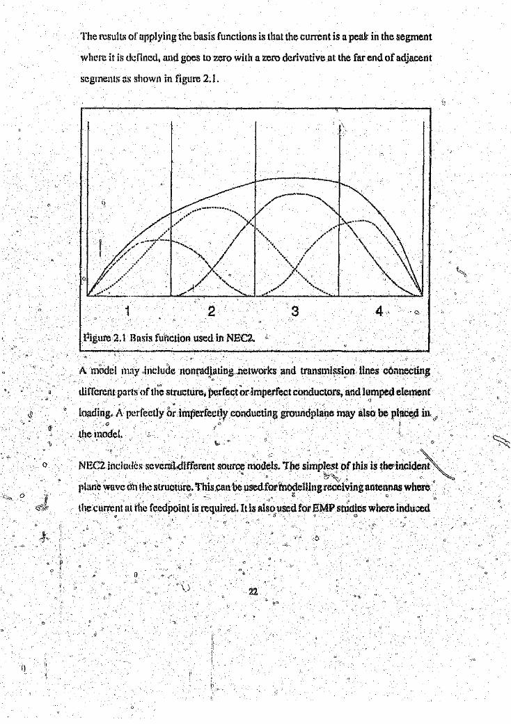
The results of applying the basis functions is that the current is a peak in the segment
where it is defined, and goes to zero with a zero derivative at the far end of adjacent
segments as shown in figure 2.1.
if I
2 3 4 'a
I~igUl'e2.1 Basis function used in NEC2 ..
A model !nay ,include l1()Ora~j(ating.networks and transmission lines c6nnectin~
different parls oftll'e structure, p(~rfectodmperfect conductors, and lumped element. .. (J
" ~~loading, A perfectly odmperfectJr conducting grotll1dplane may also be plac~dill if'
o
the model,~._,
"
o NEGl incl"tlc, s.. ve~4~4irf"relll.dur~ mod¢ls.lhe simj}l;~ OfIbis is the inCid~plane V+l1VC (tfl1 the structure. This:can be usedforfi1odelling receiving antennas whereg. ... . . ~o
thecurrent at tile fcedpoin; is required. It Is slsoused for EMP stllC1ies where induced{i 0 Q)
22
1\
c 0
currents on (he structure nrc calculated. An incident plane wave is also used in
scaitering slndies where the field scattered by the structure is examined. This is not
vet')' useD' , the present study and no further details are given here,
A useful source model and the one mostly used in NEC2 is the applied electric field
model. Here an electric field is specified at a single match point. For a voltage source
of strength V 011 segment I, the element in the excitation vector corresponding to the
applied electric field at the center of segment i i~ set to
1,1' VII --+:I
IJ
(2.20)'"
where t:.i is the length of segment i,The direction of IJ:j is toward the positive end of
the voltage source so that chm;;ge is I~u~hedin the same direction as the source. The
field at orhcr nmkh points is set to zero.
The actual effective voltage is the line integral of the applied field along the wife.D .. .. ... .. . ., ... .,
This fjel~ is not known a prlo~il3ut may ,pcdeterminedaftel' the current is found by(~". . --..... . --.- -_ . ... .
iJ~(egraling the scattered ~ield pro4uced ~Y the current. The field is nearly constant
o~el' the segment arid drops sharply at {hi segment end~. This means that the
approximation of the voltage in equation (2.20) above is approxlll1fftelycorrect.
Q
(',
The I1ntenntt Inputimpedance is ,computed by dJviding the currentlu the centre ofo . \I "~,"""
the s~~gmellt(a1isumingit to be the av~rage current) by the applied voltage.4!tneo
segment is short and a bymmetric feedpolntis,.used so that the current of the centerC' . (i
equals the average current and the assumed volt~geequnls,the actual applied voltage,~ ;':_' - . . . _- /1)
o ff
fairly accurate. admlttance, results can be obtained,"-a '-I
il
oo
23
D
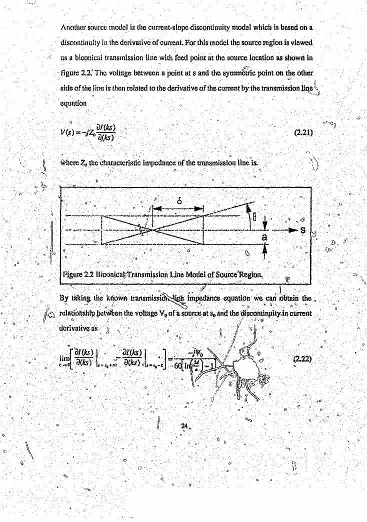
Another source model is the current-slope discontinuity model which is bused on a
discontinuity in the derivative of current. FQr this model the source region is viewed
as a biconical trnnsmission line with feed point at the source location as shown in
figure 2.2. The voltage between a point at s and the symmgtrlc point on the otheri
side of the line is then related to the derivative of the current by the transmissionliqe '\))
equation
"
whcreZu the characteristic impedance of the transmission line is.
'0
(2.21)
p 6
--~---~-~~r~~r~}~_-t-- ...s_'-. -,:~."~:::::.-----..: ... --_;------------- f". ",-;_, I) _
o'.:.'
F~,gure2.2 Bhmnicai;:Tnmsmission Line Model of Source' Region.~ .~. "
By taking the kllown· .transmissi&~~ln~" irhpedance equation' we can obtain the =':"" "_',~:',"_ '''' __ ',,' ~_""~> -. .'-: _:. _ =. \~ o 0
l'clati()l)shl'p~ctW'ec:nthe voltage Vo of a sou,rce.at So and the discotltin_,uitydn current
derivative us (f')
II
o
i~f~(~~iL:.,;;~~:-YL,,~,1~-6 ....--,.~--
24,"
o
'(2.22)

By making suitable changes to the basis functions the discontinuity in current call
be introduced For details of this procedure sec (14).
With the current slope discontinuity model the admittance is the ratio of the current
at the segment end, where the source is located, to thv source voltage. The two
segments on opposite sides of the source must have equal length and radii. This
means that this model can not be used to model monopoles Or to feed at the junction
of more Ih\~11 one wire.'\ ]ii''\n
2.4 Program THWIRE.
The THWlRE program (17, IS) is a thin wire Method of Mon1~nt~ program used to
calculate the currents 011 the wires because ofa specified excitation. Fromthe currents
several secondary pernineters such as inputimpedance, coupling between ports and
mdlJ{iol1puttr,rl1s 111uy be computed.
The program uses the reaction integral equation as described in Appendix A.\\.
The program makes use of similar basis and test functions and thus a s:>:,fl11netrical~i G
p1at~ix is crcHt~~. 'The basis nf1tt test tiJnctiol1sar~, defined over what are called
expanslon or test di'poles1 Each su6~dipole consists of two ~dJacent segments of the'
wire structure. Such a dipole can be a lineatdipole (When the two segm~nts. foWl a()
straight line) 61'a V-dipole (wh:~nthere is an angle ~~therthan 1.80° between the two,)~~. Q
segments). v.::!/r,
(j
The current diGdln;tion of It linear expanslon ..br test dipole is ghown in figure 2.3 i?.
andglven by
15i)
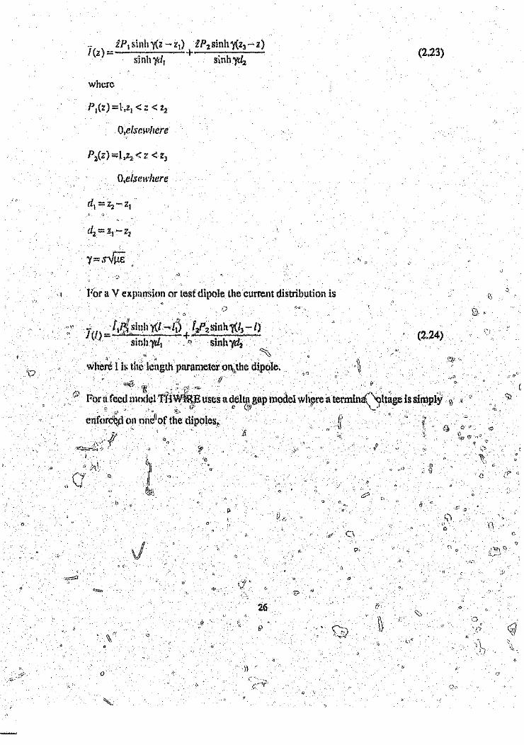
(2.23)
where
O,eis(!wlwre
O,elsm.vlwre
For a V expnnsion or test dipole the current distribution is
c
- tiP({ sinh y(t-I;") [zP:7,sinh'Y(13 -I)J (I) ;;;:...:..1'-"- ... +. . . · , .-
sinh ytil C) sinh yd'j. (2.24)
"
where 1 is th\~length' parameter ot'lthe dipole.P •
'f.{, " ' , ,~~J~:'., , " , " " , ',' , " _, '_ ' ,",For ~~feed mo~lclTfl'\.~i~E uses a qeh&!gap model whyre a termina()ltage is simply<mforc~don nnd10f th~dipoles,
\) 1\
t(III'
o
1/
V
26(I \\
---_.---------------------
------- ..... Zz3
I/'I
z1 22.. ····'1
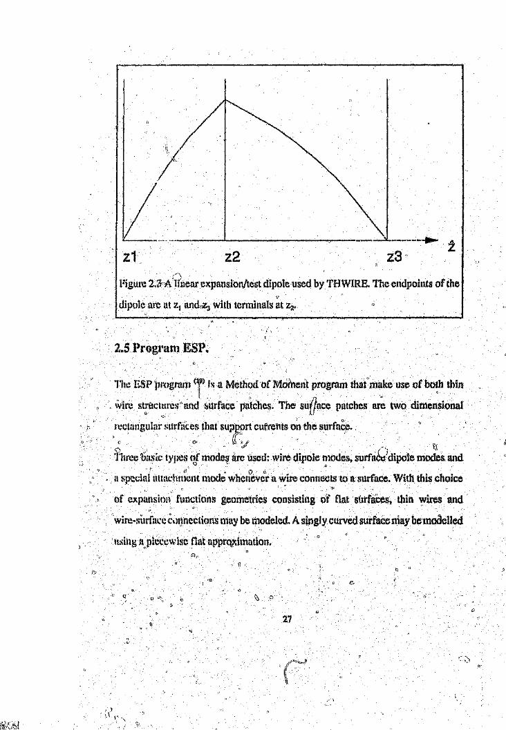
Figure 2.:;Y-AltlleUl' expansion/test dipole used by THWIRE. The endpoints of thee
dipole arc at Zt and.z, with terminals at Zz.
2.5 Program ESP.
The ESP 'j)l'ogram (~r) is a Method of Moment program that make use of both thin11 . ':i:
,vil'c st(;uc:turCH"and surface patches. The sur/ace patches are two dimenslonal
rectangular surfaces that sllp};lprt currents on t.!).e stlrftlc.c.,._, ...' () IL)' .... \.\1'hree basic types <if U1()dc$arc used: wire dipole modes. sUlfu¢t11dipole modes. and
a sp~dalatt:whn;cnt mode whet{levcr a wire connects to a surface. With this choice
of expansio» functions geometries consisting or flat surfaceSt thin wires and
wire-surfac» cOl)nections may be t'ilOdelcd.A stog1y curved surface 11laybemodelled
using a piccl:.wisc flat upprQ1<.imation.<1· -
o
"o ()
27
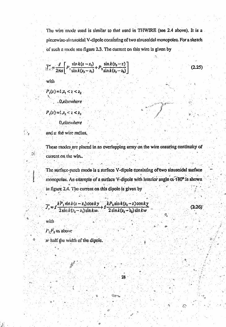
The wire mode used is similar LO that used in THWIRE (see. 2.4 above), It is a
piecewise-sinusoidal Vvdipole consisting of two sinusoidal monopoles, For a sketch
of such a mode see figure 2.3. The current on this wire is given by
--,.. Z" [Sil1k(Z-zd Sil1k(Z3....Z)]'[,=-- p . . +p .,_,_ . 2n:a I 5111 k (zz - Zl) 1. sm k(z3 - Z2) .
(2.25)
with
O,e/sew/cere
O,e/smv/zere
andr; the wire radius.
These modesarc placed in an overlapping array on the wire ensuring continuity of
current Oil the wire.
The surface,·patch mode, is a surface V-dipole consisting of,two sinusoidal surface
mOt1opoles. All cxtt111plc ofa surfaceV·dipole with interior angleol:~i800js shown
ill figure 2.4. T!lC current on this dipole is given by(;
t;
(\
with
(I cH' half ~l1cwidth ofthe dipole.
o
28
I
..JSS
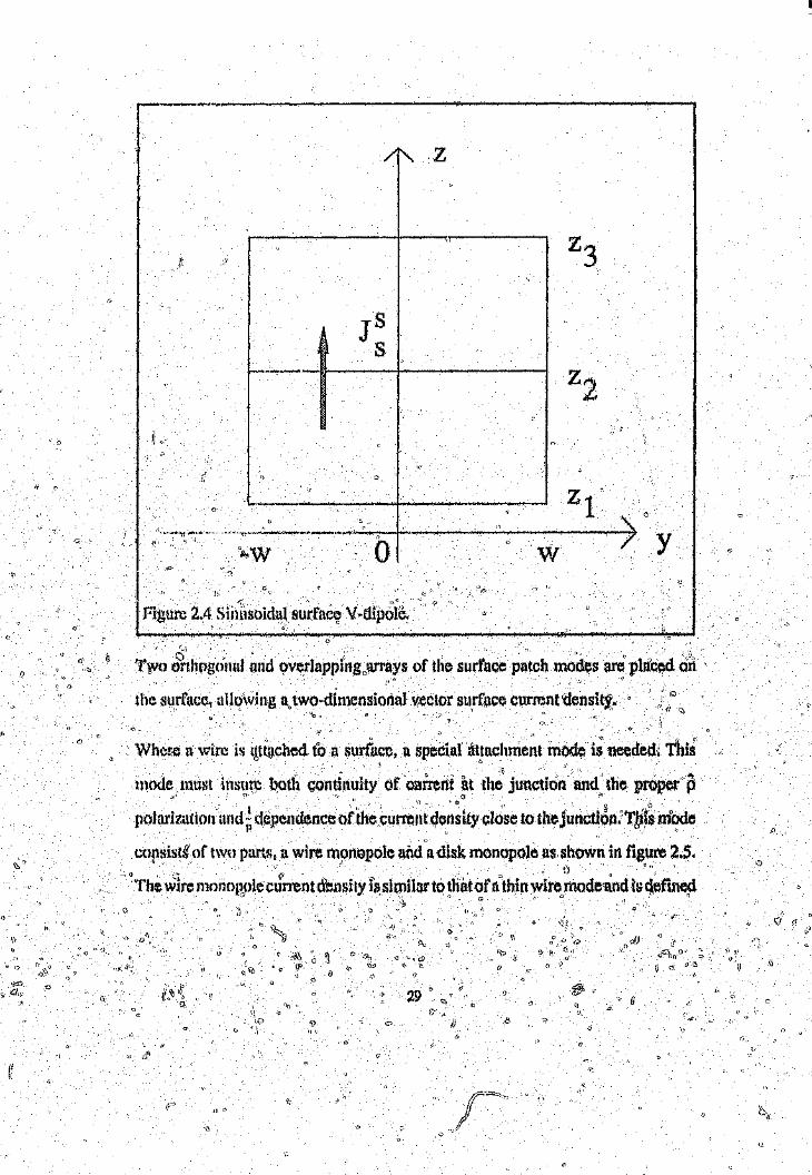
rigUre 2.4 ~iJHlSOidt\} surfac~v~~Hpoic,
'l\V() J}~lmgOiHdand overlapping"urrays of the surface patch modes are plrtce.d ori
the surface, aUo\ving aJwo~dimensi()l1aI vector surface current 'de11sit~"\: n
o " c-
Wh·;:r:ea wire is t!ttlJched to a surfhcc, a special at"tachment mOde is needed,_ thismode, mus; insure both continuity of o:arrertt at the junction and' the pf(~pef p
, . ,,';1 . ,
pofarizntion and;~dependence octbe Cllrrel~tqen~ity close to the junct.i6Jl2Tl#~m(xIc
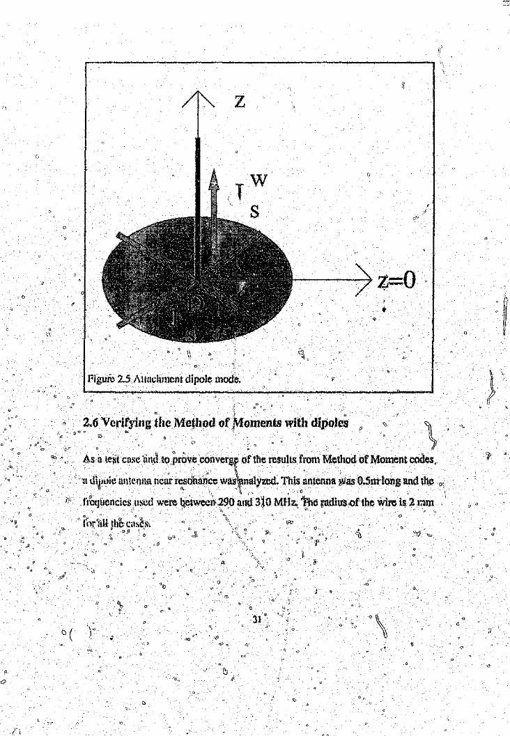
(;opsistS'of two parts, a wire menepole and a disk monopole as shown in figure 2.5.. . Uj, 0
\) .: ~. . . .. " . .... . '... .,' .....,', .' DThe wiremrmol?J)le C\lrrent ~ensity i:'ish:nilarto tha.tof ftcthin wlrejnodeand is qefincfi
"/ " . ',' . i;·. <:') " '" _,' •
i)\l 29 " (J
'.j
cj) I)
" :.I'

as
_·w i I;ink(z,-z)f ::.::..~.-.-~,,-.--• s 2nu sinkzz
(2.27)
where the disk current density is defined as
~r::.:: p_- sin k (b - p)s 21tp sink(h -a)
(2.28)
where
1.1, h are ilH~inner and outer radii of the disk.:1
AII'
Note t~ll!tthe inner radius of the disk is equal to the wire radius, thp:t the current on;1 " ')" .. \
the dhl!&at u is equal to the current at z=Oon tb~ wire to ensure contitrllity cf current! "f" '. ' ,= " ' \, ., "If
IH Ih~ju/}CLion. Th~~'Urrent on the disk at b is equal to zero toensure contim~ttyof;
current Q,I\ the surface, '1\
it \:\ _, _ '_. _ II
It is important to note that wiJ,h thep~ e~tPflns~tH1~\functionsthe, e ....t':.''''r.t it. a1way~1/ C ' ,
" ,y cOlltinUOtI.ll'1nthe direction ofth~,curt(mt, bot it pay not becontlmrous in the dirci{:liml"
f, orthogonal (0 tl.1c current flpw.(\ :_, I) - fro
II1/
For antennns the ~ame feed moSfeUs used,.mi'in THWIRE, ('flat is. a delta gap mbdel~ ?> ,," 6
where U lCl'millnl (voltage is simply el\forced 011 one of she dipoles.
d. II
-..9 .i1) 0'~:'.> a()
{)6· o
c
"c/'
';:1
d' II
o ;'1G
30 o
o\';
o(J
()
c
z
o
Figure 25.Attachmcm dipole mode,
2.6 Vcrii'ying tlw.Mc.thod ()f,~1omentswith dipolcs!) .c. 0 ,)',
.::)
As a te~t case <lIld~().pr6ve convergp .ofthe results Irom Method of Moment codes.
a,lnJ,)~)jeuntenna nom,' reS(.j,ni1~~.,ewas,knnlYtlld. ,T,I,li5 Ilt1.tenn,' 11W'as o.5m,',long and th~. ' . nf . • 0
r&qllt'mcics used were betwecI'l·290 and 3~O M:flz. ~f~heradius ,of the wire is 21ilm. _.' .... ,.- . ,',' "i.
j'{)r'hH ,the ~as~s,011
,0
o
c\
1(I'
\

'I))
Programs NEC2 and THWIRE were used in this part of the study. Because NEC2
gives several different options of feed models the differences between the applied
E-field and the current discontinuity model were investigated (see the description.
of NEC2 for more information on the feed models). For the applied E-field. model,
the effect of keeping the feed segment at a fixed length or varying the length was
investigated.
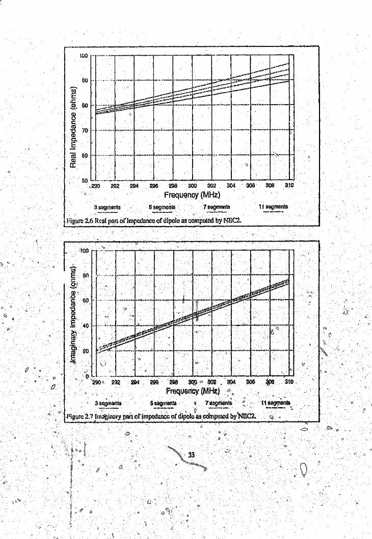
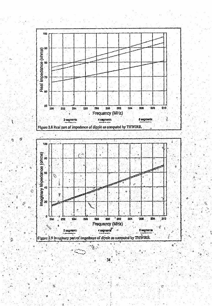
A summary of the results obtained using NEC2 and THWIRE are presented in
graphical [01111 in figures 2.6 to'2.9. These NEC2results are all for the applied Efield- 11
teed-model where the feed segment length was changed hetween: the different cases
to be t'he same length as that of the rest of the segments. These results are also,
tabulated in appendfx C.
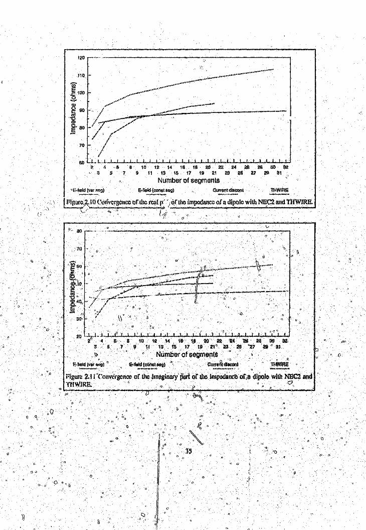
Figures .2.10 a1'l<.\2.11 show the convergence of the impedance results with both(I II
NHe:! l1tlPTJ lW~~{E.For tim NECZ results the w)~eral different antenna models used" .are shown. thilll\pSUltS are shown for a frequency of 300 MHz.
From the result,s il: is clear that the apillied E,.:rield11lQdcl of NEC2 gives very similari\ .' <Ii...
results to the Tt1'~IRE results. It can also be seen"bmt a large number of segments~j' :, ji
are l)~,Iqedbeforl~i~heimpedances converge/fhi~ shows the difficulty irrcomputing ~a g .
impedal)ce datH b~le~useof the local nature of impedances,II . it
_,.-----.--:: .. ~.,..,-.- "~---00 " ..•.••..••..••...•.••.•..••••••..•.• , :;.»,-,••••••••••, •••,.._-.-. :::;:::•__ _....~ -:;0 :-:""_-- __- ---
Ci) »>: ,' :: ::-_"..~E . _- -;::....:;.I---~:---..c ...,-_....---:::....~:.::.:::::::;-~,g_ 80 . ~~~~~ .
sc:ro"0 70 .- , .illa.ECd 60 ..".. . ,........ " •..•... ~;;'.""'"QJtt to
296 2gB 300 302 304Frequency (MHz)
306 308 310
~~ 3_S~Og_n_1e_n~ls~__ ~ s~s_e_g_m_a~nl_s ~'_.~_~~_••~~.?_~_~ t_ls_a_g_m_e_n~_~ ~J.I_Figurc2.6 Real part or1mPcdancc of dipole as computed by NI1C2.
r?rIanl·t:: 60 f'ttl-g_E 40 '
a
_ .. ~. ~ "'~""."''''''''' I<t. " ~ ..
~<; l" _ " .. w ..
Q
.~
o
* • _ ~c~ '~ a p wFrequency (MH~:.)
3sogmanls 5segmenls 7sogments i,1 sOGl'l1enls~---..Figure 2 ..7 Ima'gin(lry part of impedance of dipole as cdlnpulcd by()NEC2.~ .. : .. /) ... ---'.--,---------"---- ---"----"" - _'-",',:-.
o.Ii \J
100.. ,. ..... ".".;,; ..
.........4.,.....•..... .-~-................. ,,;"""" . .,..-....
>".;~ * ~ , ~.. "" _* .._ :::: ;:,_- ;;:. :;.."...... "' ..
................ ............ _ .."'......... _, ...", ....
... -_ '......,,-.., , ::::::::::~::~~.-z: ~ .•••••••.••.•...!-_....-- '.' I __ ~
.::--~ --- l.--- ~~r---........ , ~.~::::::::::.: ,---
OJ 1)0ocCO"0OJ0.70ECO(l)
c.c 60 ~ ~ _ .. _ "................... .. 010 _ "'. . ...
so 29$ 298 300 302 304Frequency (MHz)
306 (loa294290 292
.2 segments <I segments
Figur.e 2.8 Real' part (Jf impedance of dipplc as computed by THWlRE,
o
Q'30B aoa296 2\Ja 3Q() (,)302 304
Frequency (MHz)290 2114
)'ib;.> $GgmentG 4 segmanl,' 0 8 seglnoot$
~"~wr~~.9 fpmgl~;;;hofllnl~cdnllCCo(d;i~:llScomputed bynI~';;~:'~. 1,
o
o
\1
o
o 34
I)
o
II
o
120 r+" .•..
. , .
...................................~' 90 •••• _---.----:....- ------""" ..,.rg ... -==.-~--....::.::~=-:-- ----.-----_.------fJ)./ ,;;.,;'~ 80 f-t / /"
- ;1 /'I
//
60 U LL...1 I2 11 . (;
'10 -
70 -
nI I I I 1 I I I I J , I , ,. I ! I .,.L._L' I I I
10 12 14 lG 18 20 22. 24 21'> 211 30 329 11 13 15 17 19 21 23 25 27 29 31
Number of segments:'I 5 7
I '·E-hold (var !\1l:Ji g·tiold (conslseg) Cutrontdlscont lHWIHE
IFigllrc,~.l()COllvcrgcncc of the real p .iqf the impedance of a dip()le with NE~2 and 'mWIRE,'-----,..1<' ..-........_.,;;...~ . ,
\ •.,1 ~
---:;-·~-·~·~--'----o-------..............,......-....-------:-.-,tlo ~
THWIFle
Figure 2.1 rCouvCrg{!llcc of tim imtlgintU'i Piit of the lmpodanc~ ofon dipole with NEG2 andTHWJRE, " Q
, j)
0'
n
II f}
oo
II n
(l
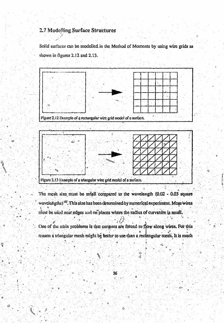
2.7 Moddling Surface Structures'j
Solid surfaces can be modelled.in the Method of Moments by using wire grids as
shown in figures 2.12 and 2.13.
Figllt'(t 2.12 Example of a rcclangnlar wire grid model of a surface.
Figul'I:l2.13 Example of n triangulur wire grid model of a surface.~--~-~ ~----------------------~~--~~The mesh size"must be Sn1.~llcompared to the wavelength (0.02 ~ 0.03 square
wavclchgths)m, This size has been <l'etel'mined,bynumeriq~l experiment. MOflcwires~ . . ,; , ' "" :,', ,', , ""'-', - , , , ,,' ",'," "" (\ -'" -', " , ' '-
Illust be tI~cdncut'.cclges :md Olf'places where th~ radius of curvature. i§ sman.'\ ,', !)
" ",' () (, "l';;Onc of tllC muin problerns is that .CU1'ljents ~fe fdrc~d to ~\owalong w~,res.Fot t.ris
co "11 \1
reason a triangular mesh might b~ better 10 use <!Jutna. redangular 111esh~,ltis muchI)o
Q
(l

more diflkult 10 form a triangular mesh than it is to form a rectangular mesh. Should
crirrents lend to flow in any particular direction then the wires in the mesh should
be directed in that direction.
The radius. of the wires should be such that the total surface area of the wires is twice
the surface urea of the modelled surface (2), By /;xperiment itwas found that the wire/1
surface sh.mld never be less than the modelled area. If the above statement is true,,,')
then for radar cross section (ReS) computations, the position of the ReS lobes will\\~. .v
be correctly predicted and the magnitude of'the tT" jor lobes will be correct. Major
lobes arc !lot very much affected by radius size. The wires should be of the same
conductivity as the surface.
To test some of the above statements, a two meter square plate Wit~la quarter meter(" •.( "",, _ ,," II ' "J
monopole lllot{Il\~~don It was selected as a test vehicly• A frequency of$OO MfIz
o wa~ ChOSCll.HS one wavelength is equal to one;;mcte~ at th15' frequency. Several
di Iferent olltiolls were tried to find .a t:~liablemethod of mQdelIing such a s!4rface.
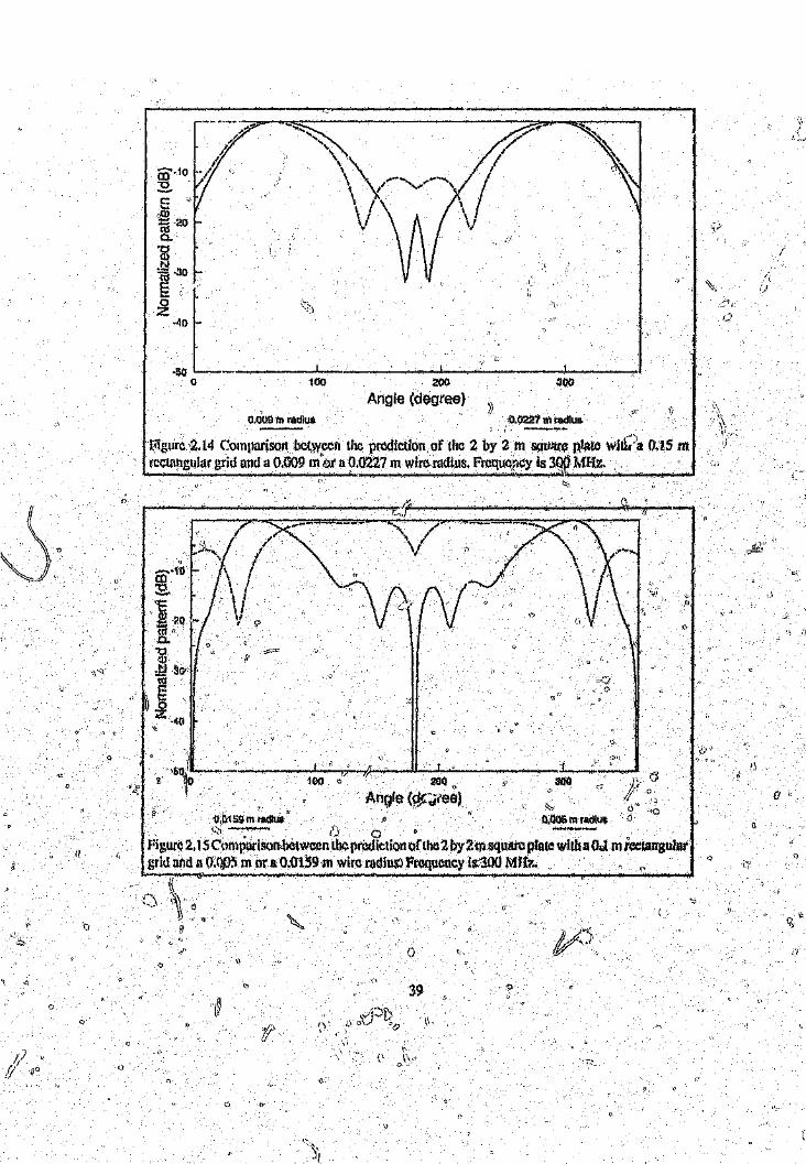
o T() dctc'llljn~' the "~eeSSnry'I'dIU~require\! for. square g:ld. a grid ~imof O,l~tIl
was chosen and. computations done at different wire radii. Figure 2.14 shows the
result for two rtldii, Itwas found thnq!OI1VergMce was achieved at a radius of abbut(J ,
O.0227l}1.The same expcl'irq,cm "VasrepA~atedfor a grid size 1JfO.lm. Results for this
case are sh,}"n il> !)gure 2.1~' From th1t~o &ri~sizesthe ~"ction was tn.de thatthe wire surface must he equal ro twiCe the sur(m;e of the modelled s.nrEnce and
nCOITe~pontl~to the rQHowingJort'll~lla (see nppendix t> fofihe derivation).
o

/I
I)
a :=. d121t (2.29)
with IJ the wire radius and d the grid size (distance between two wires).
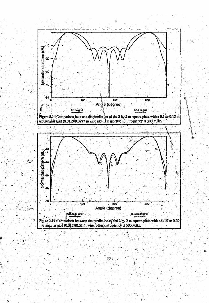
To determine the necessary grid size to use, a number of computations were done
w4tb different grid sizes. In all cases the radius was chosen using theformula above.
Figure 2.16 shows the results for two grid sizes. It was found that convergence was
achieved Itt 11 grid size of 0, lm, that is, 10 wires per wavelength.
A test on the grid size for a triangular grid,was also done. The necessary wire radius
is derived in appendix ij. Figure 2.17 show~, the' results. In this case a wire length of
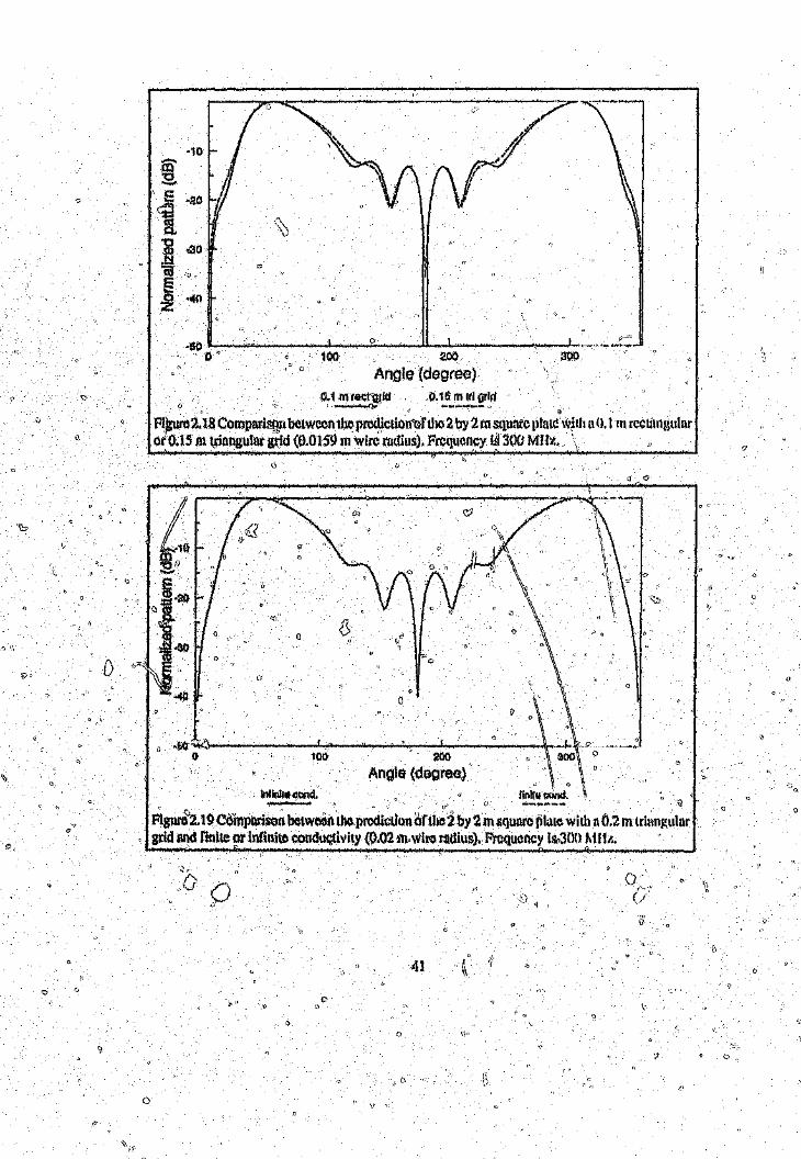
O,15m was f()lmd to be optimum. This result is compared wit~,the previous result"forthe rc~t,tnguh\!;,grid in figure 2;.1811:pd the results are nearly identical.
c ." d ..:;1 {I-
All computations we}e dQlle'unt1er the asSumpl,l()I1dun th~ pilate was made from a'" 0
perfectly cOlr~lllctillg mnteriuLFigtlre 2.19 showsihe,coIl1pm-ison between a perfectly
condtltting iJhu~ and one offinitc ;ollductivity,. No difference between the two plots
can be seen,,(, 0
'J o
c ,Tile last and most diffi.ctllt test y.tas to ci¢nlpare ~he predicted results, to measured.\1 .. aO·.· .••.. \.,0,\
o results. This is-done in figures 2.20~~o2.23 fQr a rectangular infinitely conducting
grief and in figures 2;24 to 2.21 for a. tr1allguhifTiniteponducting grid at a number of'
frequencies Gdose to 300 ivlHz. Inall cases the l'csuUS compafe widlin the typical
t.l1ecisutemCl1&,ermr~.Q
I)
38"Q
()
o
iI
~~.It____ ~ 4__~ ~,___J---.- ~ ~-
100 ~OO ~OOAngfe (degree)
0.009 fT1 rlldiut
Figure 2.14 Comparison OC!"WCCIl the. prcdiction. of the 2 by 2.m saUntc p,l;ltc wlU?a 0.15 mI'cctanglllar grid and 110.009 m'or a 0.0227 In wircnldtus. Frcqucrcy is 3~ Mfb:.
4--- ~ --~--------~-.--~~----~--~-. ~--~~ __~ __,~__~ __~
o'_'_""'_...-J-":;_~.L...-...i
s 3(!O200 <)
AnoIa <<:i,(dfee)
o
39
'o
\~
.50 _._. --..,J...- \1 --1--,__ ...IJ
o 100 Ii 20() (l00
(i,' ~••"; An'. (<logl•• ) e ~~~ c
foigurc 2.1•..·16 Comparison,}>Clwccll.iilC PtCdiCl}~n of lh.c'2 by 2.m SqU..arc plate..with a O.1..·.i;\~r().15InrCGtl1ngulargrid (0.0159/0.0227 m wire radjll~ respectively). Frcqll(.:.llcy is 300 MHz',"-_.......... .' ,
o
\\1 co
o
.;0 L_...~. ,__ ..............o _...Il.~_. ................._I_) __ .__ ..;:.L......._, __ .......,.i
o 100 o tlOO
Angle (degree)Q. . . °t~~rld . "o.2Qmlr19tid
Pig~~ 2.1;(·0,:w.(son lrel~ccn lhc prediction oJ tllC'~ l1y ; m s;;:;lii!e with a O.1Sor 0.20m ~iangulllr gr,iu (O.{~~S91O.02m wire radius)~Frcqucn~Yi~i'00MHz.
u
()
"
200Angle (degree)
0.1111 rectQ.!fd 0.15 m (tl grift-.,;- ( ~ 10- _ _
F!~ure2.18Comptu'l~n belweenlheprediclion<~r the 2 by '2m square plate Wilh u(J.t III rectangularor 0.15 .Ill tpungulur grid (0.0159 m wire radius). Frequcncy i~13()OMHz.~~~~--~----~~--------,~~
:too
o
lnllnlll; eond. ,?Flgllf~2.1 ~lComptU'ison betwool\ ll»prediclionorth~:2 by 2 m square Nate with l\ 0.2 III lrillllAulurgrid and finite or infinite conduc;tivity (0,02 ill,wire r~\dius). Frequency ISr300 fl1ll!... ~ """ {l n,...... .....__ ~ __ _.
o
\\,,\ "
o()
~------'------------------------------------------------------_'
I
IIIIII
·40 II-sl,__--...__,."L......_ .. ..,.....:l ...l ...-- __ "'-- __ ...-_
o 90 sao 270Angle (degree)
", '~"Moasurtl!'T\otlt NEC2
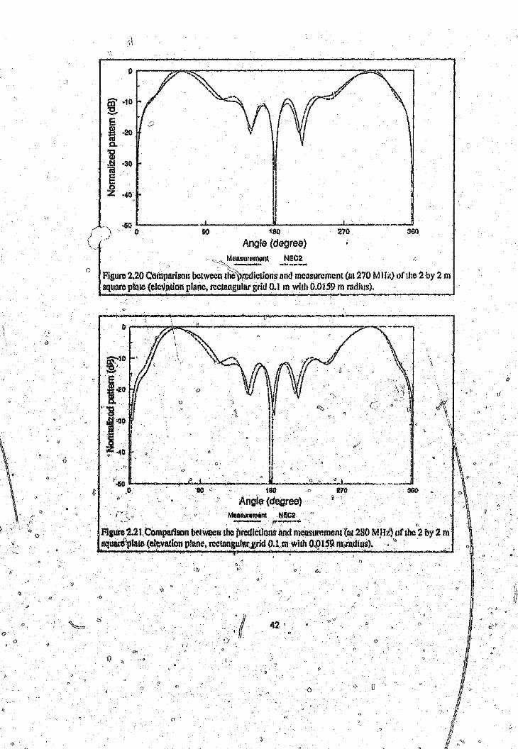
Figure 2.20 Comparison between r.ll(f\)(:cdicti()us and measurement (m270 MIll) of the :2 by 2 IIIsquare p~nle(elcvulion plane, rcctangulttr grit! 0.1 In with 0.Q159 In radius).
iJ
~ ,.!f"'''''''--- ....Figure 2.21 Compatison b~~w,(X:utho l~redictlons tlnd measurement (tit 280 MJI i) (}f thc'2 by :2 IIIsqum-e>plaw(elevation plane, rccfungulnrJtrid ().~,m with 0,0159 n'hmdius). ..',"""'---~-_""--"""'--~~'--"""-----""----.....~,,.,... ..........~
42 ' ()
() o
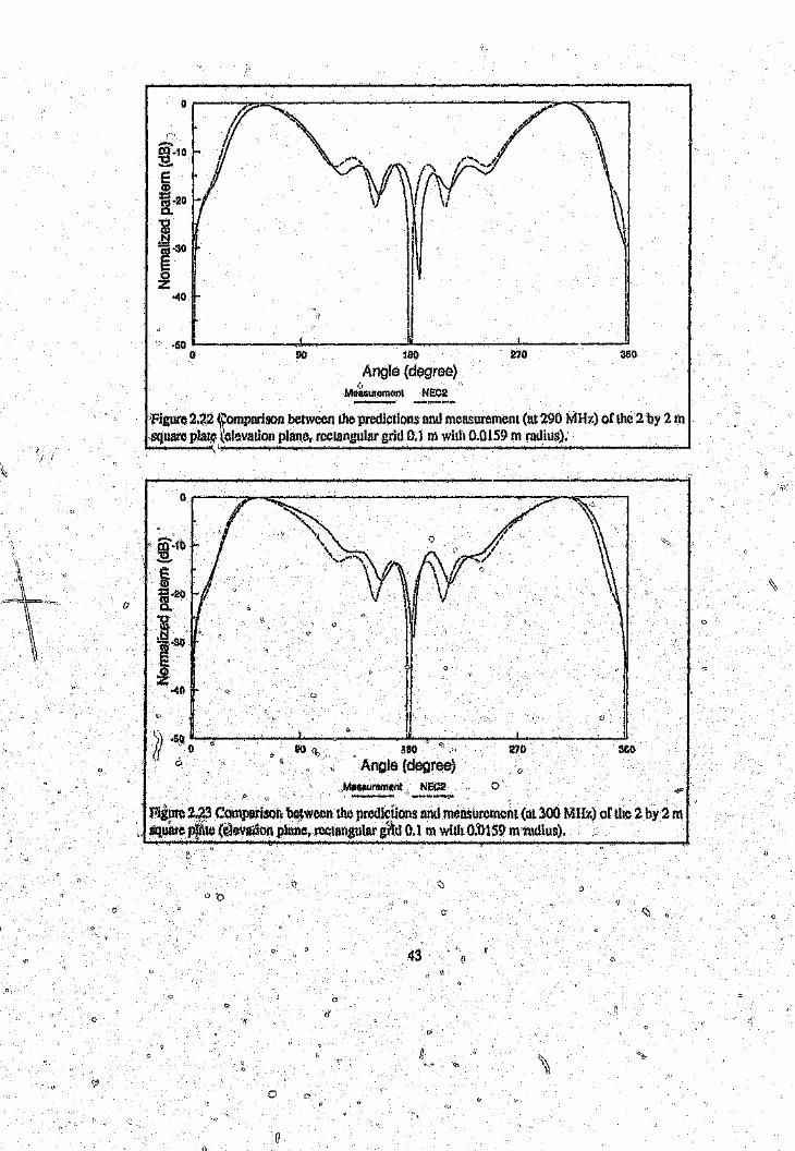
Figure 2.~2 ~~()mparisonbetween the predictions and measurement (at 290 MHz) of the 1. by '2 msquare pJau;~e!e\'ation plane. rccumgular grid 0.1 m witl) 0,0159 m radius).fo."... .....", '
o
.-..00·10:E..E~'20a.
~'«i ·30EoZ
-40
~III
iIII
II.50 J-- __ • ,L..... __ ---_~_,...:Il-.~-~------'---~-----.,
o 90 iao 270
Angle (degree)Mo'asufllment NEC2
360
l
:lElO
o 0
43
/1
o
c
.50~'"~ •__ '""'-_"""'_""""' _ __"-''''''''' ''''_____'...J.-_ ........ .:.-.-!I
o 00 MIQ 270
Angle (degree)o
Figure :2.e3 CotnpariSOIl> b(!lweCnlhe predidions and mensuremelH (ut300 MH:t.)or tile 2 by 2 msquare p~1tI (c'Jovlfuonplane, rectangular gftd 0.1 m with 0:'0159 mmdlus).-- . --~----~--------~~------~
0
-CO ·10"0-c:....ill ·20 l-1ttl0.."0Q).~ ·30 -(U
E0Z ·40 -
·500
II
II"IIII
Iuil
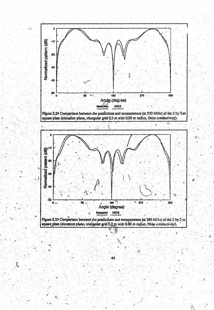
Figure 2.24 Comparison between the prcd'lctions nnd measuremcn; Cm 270 MHz) of the 2 by ?mlsquare plate (elevution plane, tnangulnr grid 0.2 m with 0.02 m radius, nnite conductiviL}'),
90 180
AO;Jl~(degree)Y,J~
Moaso(oo NEe:!
~\\
\\\\
\\III!I!jJ
.50 ,..._..._.......-..J.,.,..._....,, J--,=-_. _._....:.----.l-_.~_'".~,.-.-~<.~.0 90 \\ ,,1;1)0 .",~ c 270 . 3fiO
Angle (degrea)(J Malila\lreC NcC:?
_ """ c
o • "., ,Fjsur~2.25 Comparison betweerythe predictions nnd measurement (ttl280 Mllz) of the 2 hy<!III$qu~~;Plate(elevationphme. trin~8ulur 8d(fb.~):nwilll 0.&2m ruqius, l1tliWcOII(.lut·LiviLy). '
I,}".\!t -~_,c
-....-¥-....
I'
o
()
44
D
o
i\\ \,
If
m·10:E..EQl~-200.
~'30CO§oz'~9
'60,,~~~-......__~- ••--_Ja so 3GO
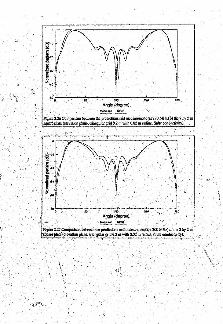
Figure 2.26 Comparison between the p(cdiclioits and mensuremcn; (at 290 MHz) of the 2 by 2 In
sqllar(~ph.\w;,(elevation pb.ltle, triangular gri~ 0.2 m with 0.02 III radius, finite conductivity).. . ~"'-'-.""--
lIl0
Angle (degree)270
II
-SO _----'--- ~-':..-........L""_.~_, ...o
l
')
iJ"-"-::::;:.::;~
taOAngle (degree)
MIII'I#urod NEC2 :'-:-:
. ' .' ,
FigUre 2.27 Comparison between the predictions !lnd mcasu(cltlCllt (m 300 M Hz) of the Z by 2 IIIcsqllttre'plute"(elevution plnne. trh.mgulnr grid 0,2 IIIwith 0,02 In mdius. I1nitc c(juducrlvny}.
45
---

" \\
o
2.8 Discussion
A short introduction into the Method of Moments was given. Severnlcomputercodes
used by the author were described,
To verify the Method of Moments several impedtltlGextudies on u dipole were done.
The best convergence of the impedance datu was rbtml1using NE<;2 with an applied
E~field source model. The solutions Were within tt few percent of the final solution
when about 20 segments per wavelength were used. It is concluded from the 'i"Jdy
that care 01) "',be taken When impedance calculations are made using the Method of\.
Moments.,
A study t6 detetmine the necessary grid spacing and wire radius for mo&mng
'Surfaces with wire grids wa~ru;f6rmed. From the study it was concluded ,l)ut there
is no sjgnif~ant) di'fference between n rectangular' and fl triangular mesh. It C'U1
fultllennore be conclucteQ)hat a wire grid size of a hundredth of a squnrewavcleugth(";:-;::.:.;::~~
.,isade'" . forraaiation pattern...stmJies. This corresponds to a wire segment leng,t,h" . f.·.r"." ,(:, .. '<--"j ...---
oht ~ ; i n wavet~ngth font rectangular grid. The radius of 'Ihe Wire n1u~ibe St~chI)
tIi~\~h~ totnl surfage oral! the Wires are equal to twice the surface of fhe plMe being".' . . ':C.. (j" ')) f')
1/ . - _.__. ~! . '. ' '" . - . . ,,;'':;1
medelled, Th~s means tftatfara rectangular grid, the radius must be 0,159 times the0" ,_, D . ""t." ". I," .' ()
G 0 ~
~ire' segment lerfgth !I'~dtor it trlm!,glllHf gri~"O,09time~ ~le'7wil'esegment length.
G '"o (; ~ \\,1 \'N'0"
(I
o
()
46
c)

3 RESULTS
3.1 Introductlon,
Tile results obtained in the modelling ora ship are given in this chapter. This chapter
shows the typical results that one would like to compute namely radiation patrerns
andcurrents, Because anhe massive number of segments (modes) needed for a large
structure such as a ship, the study is started with a greatly simplified model and the
model is !:,'l'uduallyincreased in complexity.
3.2 Geometry of ship.
G '.
The geortietry of the shipeonsldered in this stU(),)' is given in figure 3, L Please note-,~,:::::::::!/
thn.t,this sb!p is, nqJmdly a l/l$Ormodel pf n.typical real ship, but the dimensions was-'. '. \) . \ i
o choseh So that measurements icould be made in un anechoic chmnber. The scale was
'" chosen such that a frequepcy .of.'i Gl.fz represents a frequency of 4.0 MHz in the'Hll"-:;'\ ',,/. 0 (J
1
1"::,:.," hand on the ship.
\
.j\115)j:\
III'~ 0
~ . \1:'~\~.3First mritlel. (Model A) "tP /)
\~-\ 'J 0 '"
'\~, '0 "',,, \:'
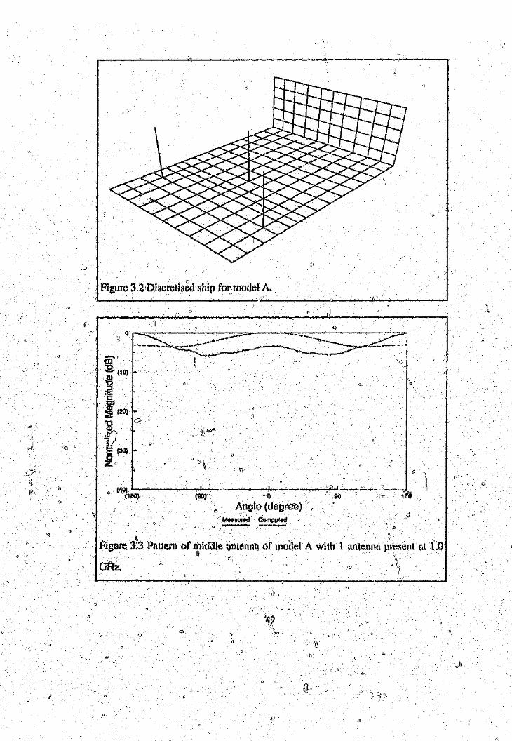
A dt~wlng,()f the flrstmodel is showll in figure 3.2. tflHs model (rnly includes the
nnte~nplatf~~m ~hdthe verticn{plate representi~g th~,firsiIl'igh;r d~~k. The model\\ ~ _-_... - (). . .: '
was disd'retised for ~\'maximum frequel\cy of 4.0 (a-It, A to\ll)1()f 409 segments ant"
::;:,(1
\
()
~s.ed in this model 't~ the ship. ,\\lith ~ segments uS,'ed fOl"5nch antenna represented'1", t;;:), ' 'c "on me ship. ' o" ,
47
<:
If-
o
........---------~~-........------ ........---, ,,,,,-,,.--'.---..
D
__.__,'_, .~.~ ~ ~----~-------t~C)-I
'.~
64. .-.~.-.~.~.-.,_.- _.d._ ....._. .-.-.~.-.-.-.-.- .... -.-. .-.-.-.~.-.-.-.- G._._. _.-.~. _.•.
o
TOP VIEW o
'u132 27/L20 .,~-rJB
All dimensions in mm
24
8032
1-....,.......... ,
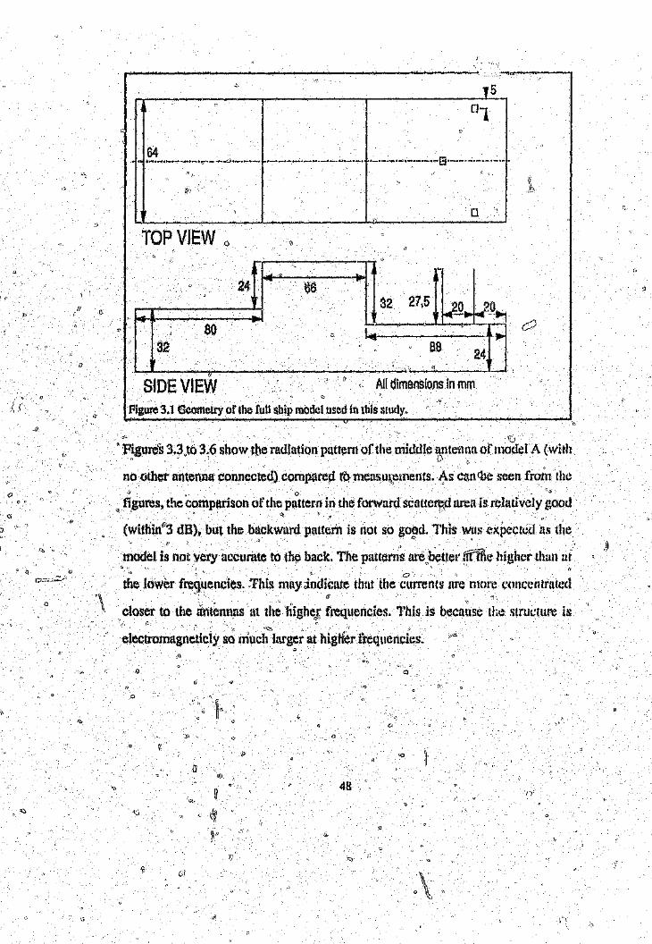
SfDE VIEWFigure 3.1 Geometry ofihe full ship model used in this sludy.
\..o Figures 3.3,to 3.6 show the radiation pattern of the middle nntennn of model A (with
" . . • !) .,
no other antenna connected) compared tu measu~einents. As c~n)fbeseen from theo 0
. figures, the comparison of the pattern in the forward scauere,d urea is relatively good,,1,'. c;.',', .. ' . ..' .' Ic'
c,
(wUhin!?3dB), but the backward pattern is not so good. This was t~xpectcd as the, C'
model is not very accurate to Ih~ back. The patterns Ul'e,!beUel' fff11~ehighet than tit'. , a", 'J
the lower frequencies. I'fhis may Jndictlte thnt the currents are more eonceturatedI . ~
closet to the ~tntemms'.at the hjghct~ frequencies. This is because the structure is
electromagneticly so mucI;'larger at higHer treqllenc.ies. ,,~
o q
oo
~,.
a\\ 48
\\
Figure 3.4'Oiscretised ship fot.model A
II~----.------------------~~------~~-~------------------~(!
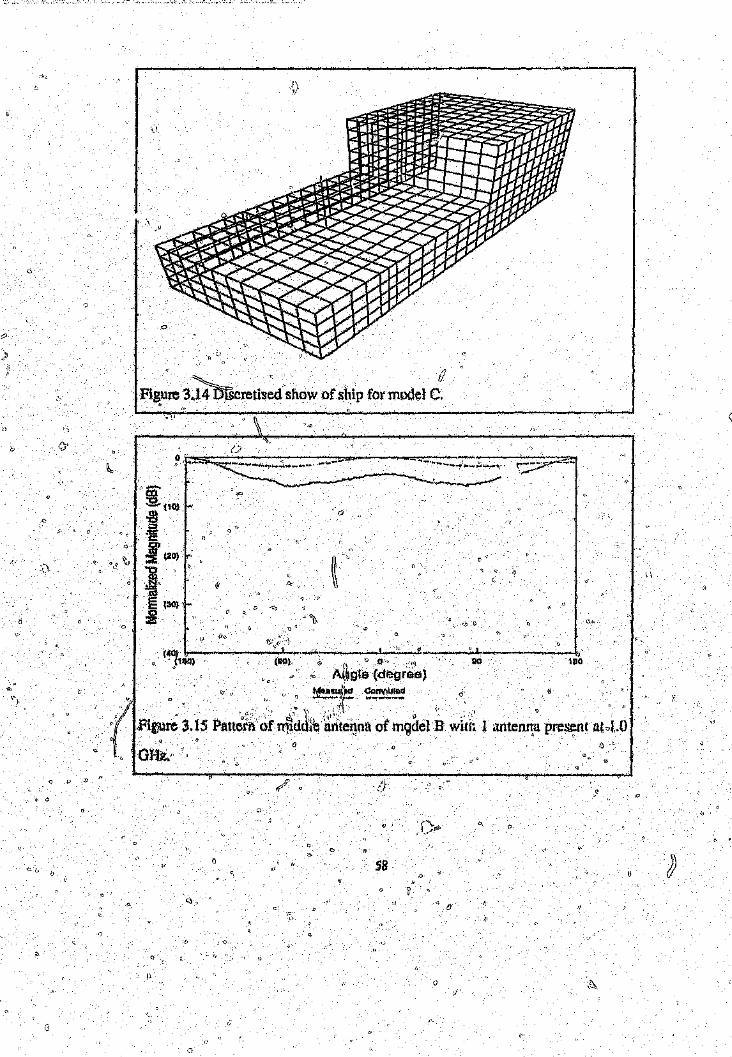
l~ ".. ".... , " > _', ,.'" " " , ", ' q ',' ," ._._ _ ,_,_Figure 3.3 Pattern of middle antenna of model A with 1 antenna present at 1.0I)
GHz. 'D
"49
o
a
co'0-(10)
J~::J:t:!c:t'Jl~ (20)
i.~.«iE (30) -oZ
{40)(lila) 90 180(00) o
Angle (dog reo)-....,-_..•..._- .. ...._----
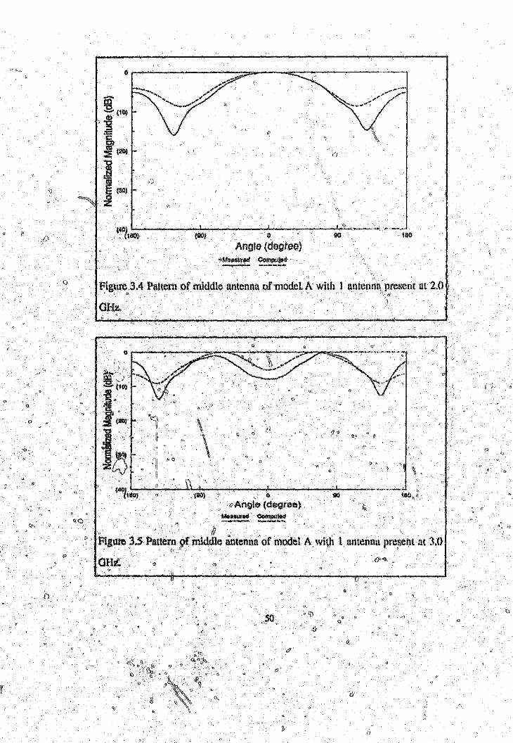
Figm'c 3.4 Pattern of middle antennn of model, A with 1 antenna present at 2.0
.J.,,;G.......I_1z......, ...,......"' __ . ~__ .......,..,__ - __ ......... _ ... ' :_ _j
.. ., ()
Fig\lt'e 3.5 Pattern 9fmiddle tlntenna of model A wi~h1 antenna pre~et1t at 3.0
.50(r
Q
o0,\
(J
o
ttl:9.. (101Q)-0:::l
:2110)'
~ (20}
"Cre.;;§ (30)o:z
__~ • •__,_,_-J- ~ _
oAngle (ds'~h~e)
(40)(161) (110) 00
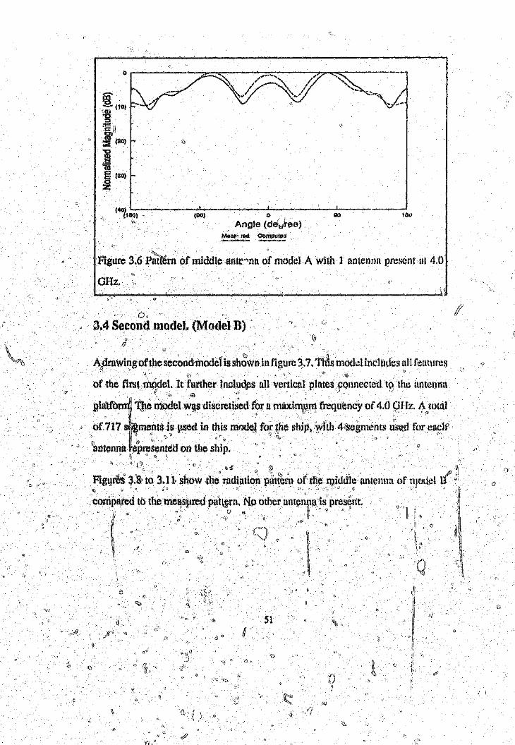
~"Figure 3.6 PlttI~rnofmiddle antr"'na of model A with 1 antenna present at 4.0
O.Hz.,_,_-----~------------................. ,----,------------ .....\ \c
0"J.4 Second model, (Model D)
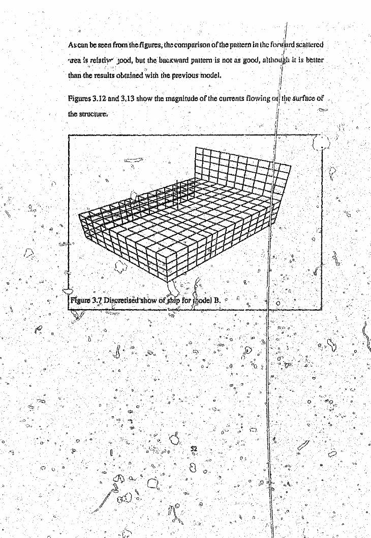
Aiprawingofthe second model isshown in figure 33. This model indtldes all Ieatures';,
of the firstmq,del. It further inclu(.tps all vertical plates connected Ip the antenna" \'.1)
phi'tfOn~i t:he n100el w9/sdiscretis'ed (or amaxirqpm frequency of 4.0 PI fz. t:- (null(}rm S~Jl):n!~J~r.se<l in ~i~mode!{ofllle .l)ip, \Vlth 4<;0gn",?" ti.'.Jl for~aplf1.lntenna ~¢presentetlon the ship. C
\\ - Q
tI ([ ~)" (!" . . . . .. ,{!
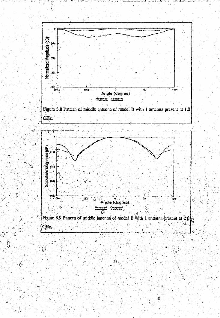
Figql;i!tS'J.g, to 3.11, show the radlatlon p~hternofthe middle nntenna of model If.:.; .._ •..'., ... " .. ' .... ":. . ... /!.. ._
I'Ii "
\)
o
'(")
'1",\
"
51!f
II~~l
!'I
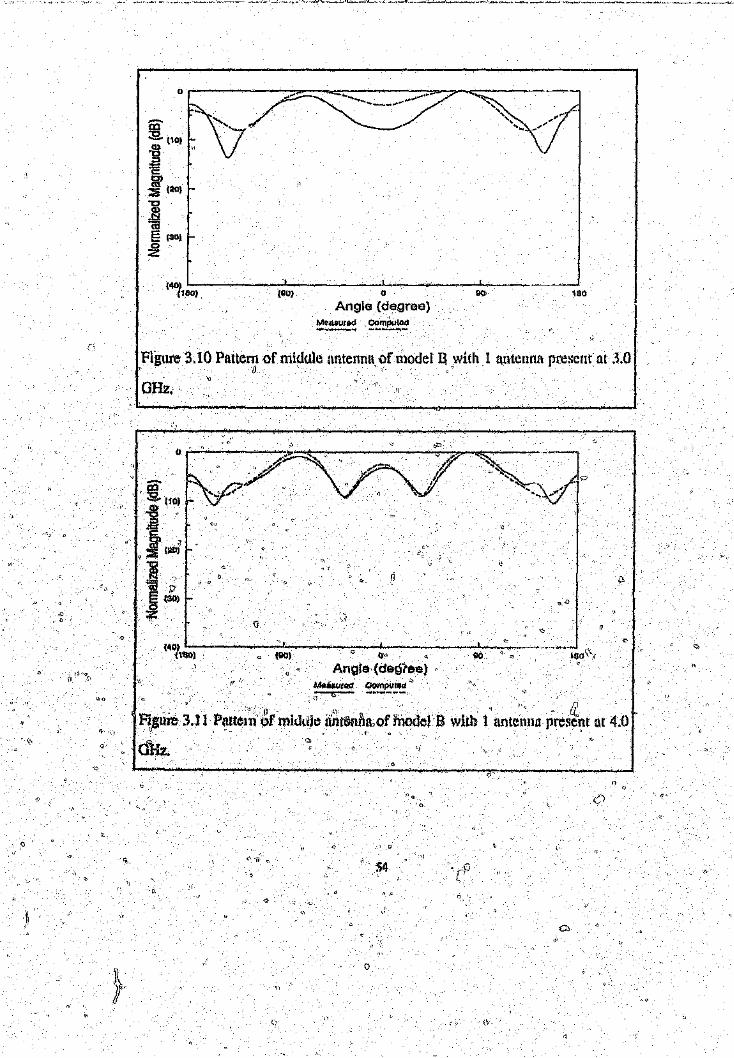
Ascan be seen (rom the figures, thecornparison of'the pattern ill Ihe ron/i",] selt[lCred
-uea is relativ-' ,.iood,but the baczward pattern is not as good, althOtlJ~h it is better
than the results obtained with the previous model. if
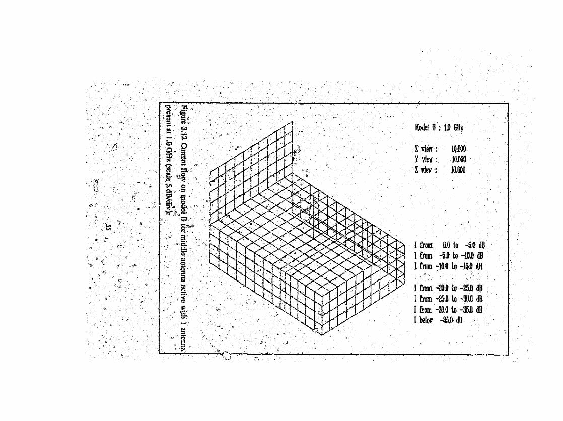
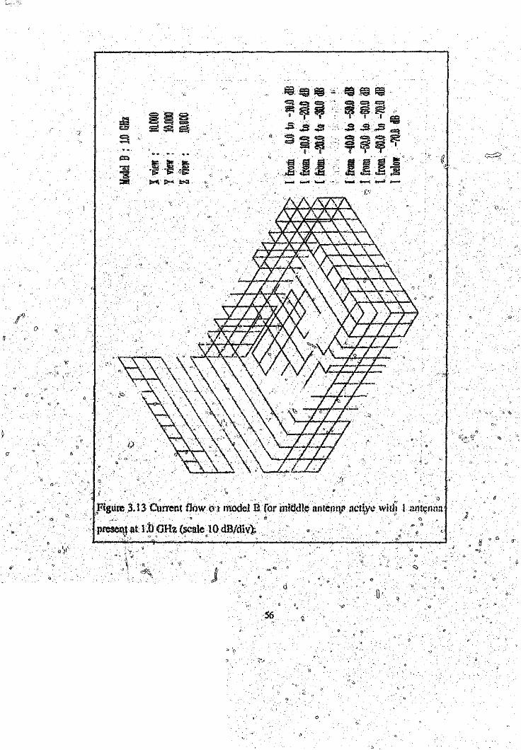
IFigures 3.12 and 3.13 show the magnitude of the currents flowing ()~ilthe surface of
the structure,
Q
o oQ
Q
521\,
o
o
,()
°r~ .....,__.........__..._--....-~---._~--~ ..~-:::.,;--=---
>J
/) . (\ Q
Figure 3.9' P~tterll of tl'tjddle t\n~~nmlof model n ~hh antenna lli'escllt tlt Z0 "
OHz.co
(40)(1M) (J
Angle (degree)00 1130(90)
MOQsurud CQmpulod--_.. _ .....----
r:jgure 3.8 Pattern of middle antenna of model B with 1 antenna present at t.n
,--~--------------------------~~------~--------------,~~~~~c~----------~----~------------~------'-----'---------'----------~
o "...
.
'"4",/
, ~\ c:;
'(40)'~'------ ........_~_~ __ ,.;;o ..... ,_._._._~...--.L. __."_, ..•Cillo) ,; }!M» (1.. e ~
,Angl.e (degree)llhJ
()
-m:g,. ('OJ.~:EL::0)
~ (20)
'"0
.~(ij§ (30)oZ
(40)'----~.(1110) (91J) o
Angle (degree)~(,Cl$Ur~e ~~~3.J!'.:'
131)
Figure 3.10 Pattern of mid(lle antenna of model 13. with 1 antenna present at .1.0(I' . ,
-o
OHz.
n
<.'-,
,-,.:)
(4°l'.li;;;--'--"'_~-i-'1l0c...l-""""---::--""Q-'~------O-LO-"":'·'-:-"-·'" '-"'HIO';',·
Angle (degree)M .. Ii.Vfolld COmpUllid ,)~ _ ..-.._- ....-
. n11,gure 3.11 Pnlt¢lti 6f middle drltlSalhLt.of roodelS witb 1 antenna pres~'nt at 4.0 ,.
()
54
o
c
Model B : 1.0. GHz
w.noo10.00010.000
){ viHr :Y view:Z view :
o I) to -5.Ct dBI from . . -10 0 dBI from -5.0 to ,r from -10.0 to -15.0. dB
200 t(1 -25.0 dBIfrom ...f %0 to -30.0 dBI rom ~~ , ~ dB
I from -3(),O to -3~.OI below -35.0 dB
o
~ .. ~~q Cl> c:::::.7~~..s;;"s~ .. t?-.¢!S~
I t
,~ S S..g..~.~it· ~ ~"I>' "S:: "5=~ ..>-t ..~
,figure 3.13 Current flow ('1 model B for middle antellqp nct~yc wid:l
present ar 1:0HHz (scale 10 dB/div);.\, " " '. ,.
o
j}.p
56

3.5 Third model. (Model C)
A drawing of'tne thi~>lmodel is S_tlDWll in figtlf~13.14.This model lncl udes aJl featuresII < .
of the previous model (model B). A further addition is the highest deck .including""
the.,ve~ical plates connected to it. The made] was dlscretised for a maximum
frequency of4-.n 01#:. A total of 1287 segments are used in this model for the ship,
wit)14 segments used fot. the antenna. D
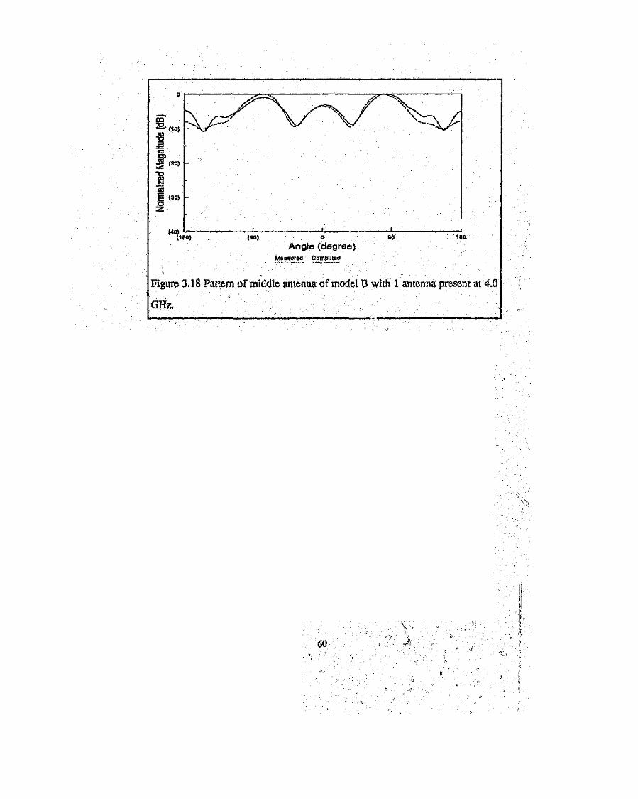
Q_ _ _ _ _ ,' __ -" ',- _ _ _ - _ _ : __ _ _ _ • 'r' _ _''' _', .' __ ', _ - _ _" __ " ,\_\FigUres :3.15 to 3.18 show the.radiatlon pattern ef the middle antenna of rmw;j C
/"
compared to the measured pattern with no other antenna present.p
, ~~n beseenfrom the figures, thecomparison of the pattern in tlte forward scmwredI .lr· . -' "'.. . .,.. .... .. . -', 'i
(, areaJs relative good. but the backward pattern ;S notas ,gtmd. Tll0°rCslIlts do noto
differ significant from those computed using model B.
0, )\ n
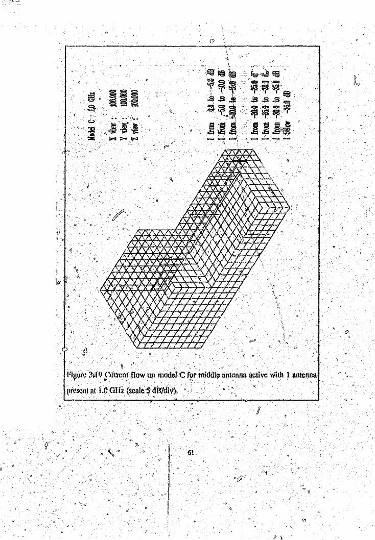
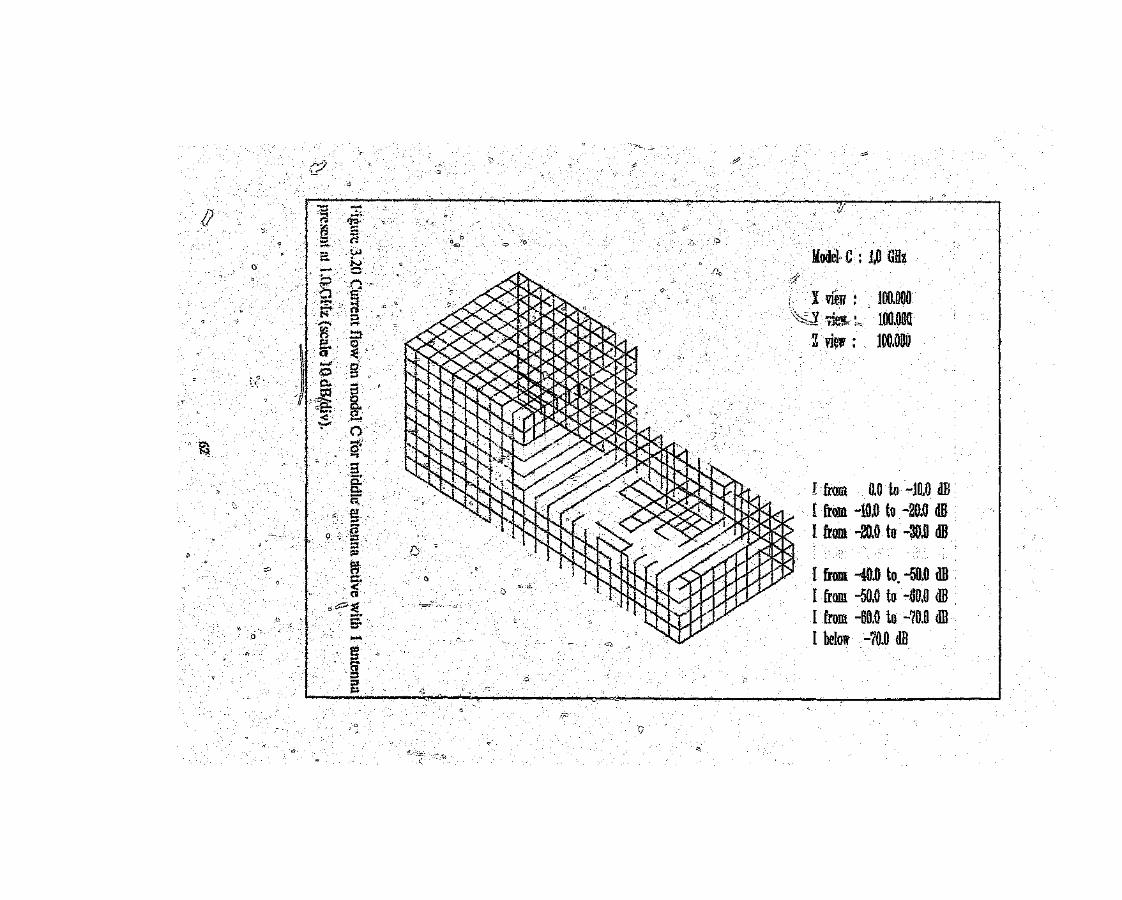
Figu~{!~3.H),Jl!ld 3.20 show t~e magnirude of the ~~\f,rentsflowing on the surface ofI'"~I
the structure.(I
(?
o \)
o
(1tJ/
<I
o
o
o
o
o o
Q
n"0 . 57
o
I)
<.,.. . {!
Fi~,ure 3..14oi"$cretisedshow of slli p for model C;
!'1"'.~Il~~~~~!.II~ (J
• ,.......... < ,:0 Y i\J\;'\.. 1 • ... ,.'
Fig)ttre 3.15 Pattern of.111'ldti'le ul1teill1tt of mgdel n wim 1 antenna present nt,,1..0(]
a 58
(I
\1
o
o
(00) ,(l
Angle (degree)00 100
MaLl.urad ComplIlqd--_. ---- ..........
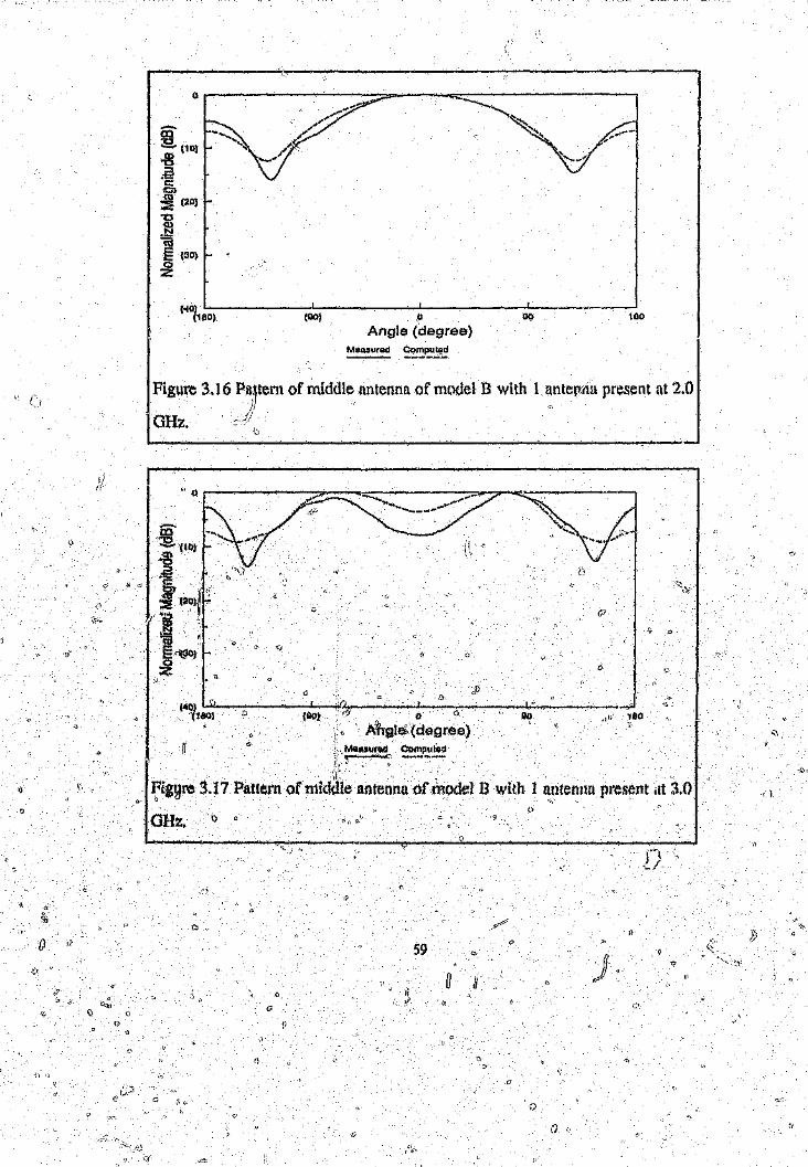
Figure 3,16 Pll,ttern of middle antenna of model B with 1 anteuna present at 2.0li
OHz.
r?
I)
~--~l)----_'·~{~OQ-l'-'~~'-'------O~----~---·A~gle.(degree)
.MQA.lIf(\d Compl,I",1;!~: ------j!,<'
.1" 180
..(t'igyre 3.17. Pattern of middle antenna of modd B with 1 antenna present itt 3.0
GHz, \)o
59
IIo
OJ:E- (10)
-g:t:::c;01~ (20)
1E (30)o:z
o -. , "'"
(40) l__(180)
L_~ L_ ~~ ~
1110) 0 91)
Angle (degree)~~M"red ~~'!P~.:"~
180
Figure 3,.18 p.at~e.rn of middle "" Of.m•..ooel13 Wit..". I antonn." present ft.! 4.•0..·•..1··
GHz. . . J
cO<.,
t)
\1'l:igUl~31'19Ctft'l'cnt flow on model C for middl~ nntenna active with 1 antenna
.C (( -v,
pre~-Clltat 1J) olIi (scale 5 dBldi'J).. ,;
o
~ ~\4 ......... ~i'\
61
c
I)
()
_,-~ >,
~ r~~'Z\? 2g~. ~:::.
~
~~c- ..,
~ dN :::I........ .....~ !:1~ 00 ~......... d'.0 ::sCl. ac:!
'.~~, 8-0-c .,'_"
":"'" o~-'0'..,
t-.~5:Q;.
G:'~:J:(;i:::!:::I::;
~,..,.<~("9
o
I
'/
Model C :. 1,0 GHz
17 ',\ V1Jj{ : 100.000100.00a100.000Z fief/ :
I from 0.0 to -JO.O dBI from -10.0 to -20.0 dBI from ~20.0 to -30,0 dB
Ifrom -40.0 to, -50.0 dBr from -50.0 to ~60.0 dBI from -60.0 to -70.0 dBI below -70.0 dB
(:3 .
o
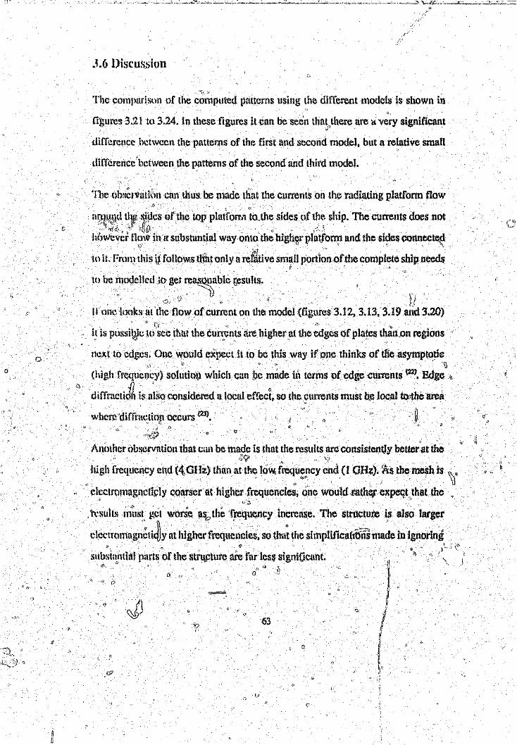
3.6 Discussion
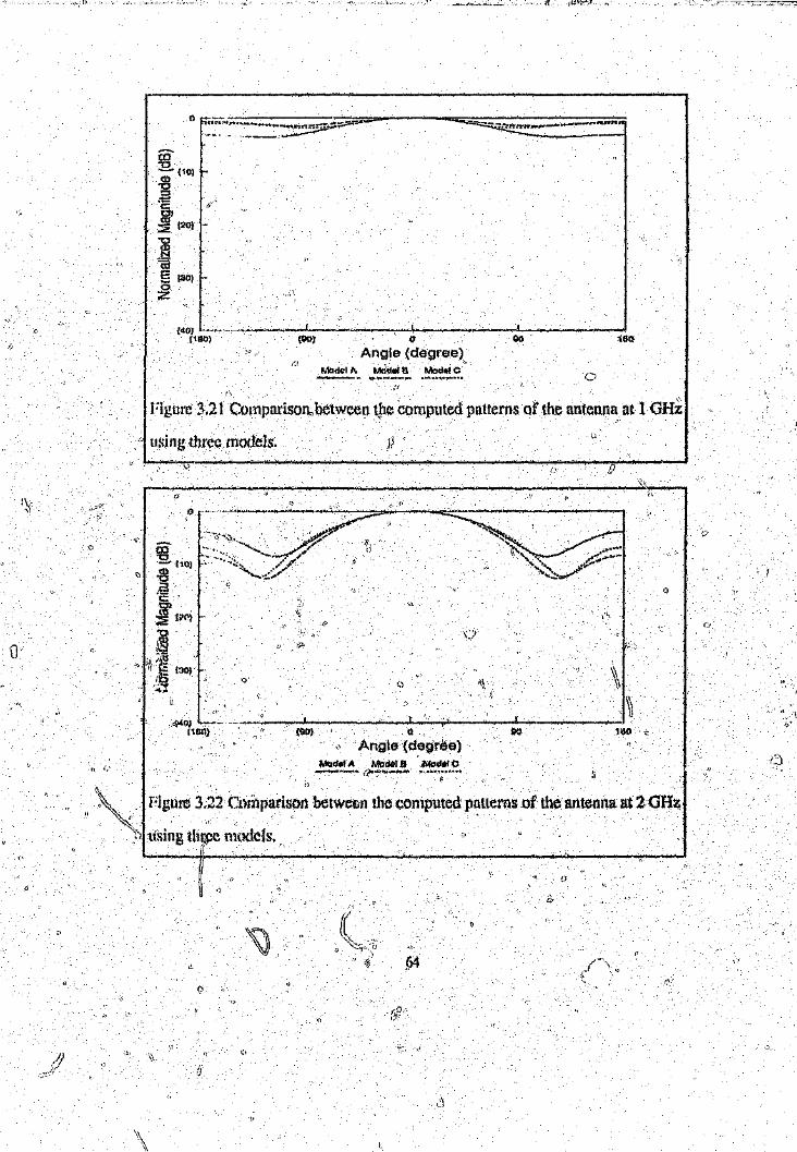
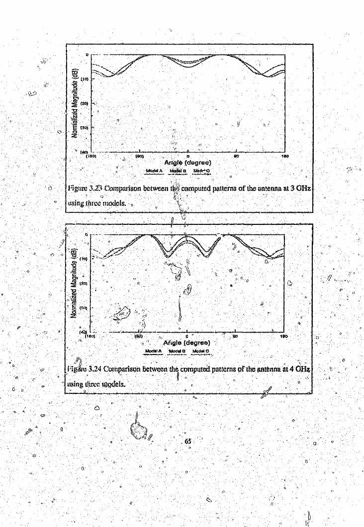
The comparison of the computed patterns using the different models is shown in
figure:! 3.21 to 3.24. In these figures it can be seen tha~:)there are ((.very significant
difference between the patterns of the first and second model, but a relative small
diffcrertcebctween the patterns of the second and third model.
The (}1)HCI~lHi6ncan thus be made tllat the currents on the radiating platform flow
m:2\~}d tl1r? ~}~lcSorllle top platforra to.the sides of the ship. The currents does not,1j':;I'd>~ II' -;[\0 .: .... . . . '.' _ ." _ . 'i .. '_' \--; -\
h6wcvcr n(n~ in It substantial way onto the high<Erplatform and the sides cot1nect~\~\l
," Mto it. Frumthi» tt follows tlrht only a relative small portion of the complete ship needs
I'
UI! onelooks at the flow of current on the model (figores 3.12, 3.13, 3.19 ai\d 3,20)
,-,
it is possiljle to see that the currents arehigher at the edges. of plates thall,.on regions.~ ., " ,
next to cdggs, One wnuld expect it to. be this way if one thinks of trfe asymptotic1\
(high frequency) s()tutio~ which can be mnde in ter11.1Sof edge currents mJ. Edge
diffracti~ill is also considered a local effect. so the currents must be local to-the area
where 'dirrractiojl occurs (:m., "!
,;
Oi:(:·~'Another observation that tail be made is that the results arc consistentlY better at the
~9ihigh Irequency end (,tGHz) than at the lowl frequen, cy end (1 GHz). A.sthe mesh IS \\ 'I'
'~~ '. '\)elcctromagnctkly coarser at higher frequencies, one would rathe,r expeqt that the
" ..... . . . ..' . "
h'sHlts mnst gel worse as:,?the 't:requency Increase. The structure Is also larger
dC(.'tnmlagnflk1Jy nthighcl' frequencies, so tlT~~the sitl1plificabt5ns made in ignonngsubst'~l1thtl parts of the strq~ture are 'fur les;l signi{icaot.
t:: \}
a
o J)63
r}o
co-0~(!O)
-0..gCOJ~ (:?O) -
~.~E (30)o;Z
I.l
Angle (degree)160(QO)
Figure 3.21 COl11pal'isofi;.bctwcen tIle computed patterns of the antenna at 1GHz
o
using three models.
(lIO) uAngle· (dagrFie)
M<ld.' A ModOI El. ,Mod.' C.--- ,~- - C" " ..
• I
Figure 3.22 Cmilparisoil between the.computed patterns of the antenna at 2 GHz
using til(,}!cnrodels.
r
(IIO)(i601 QO 160o
Ang!$ (degree)Modol A M(ltlal B MOd".'O---- ._- ".._.- ~.,,...
Figure 3.2'.1Comparison between thl;Y Ct~mplJtedpatterns of the untenna at 30Hz
Hsing three models.
o /)
. :'\~/,~,,,-.."__-l';; _""_...,...._~.__ -L__ _.~_....,!\',",' ___.
lob} 0 . uoAf,~la (degree)
(nC)J •.(160) 180
1.<'\f
/fjj(:igclre 3.24 Comparison between th~ computed patterns of the antenna at 4 GH~
, II " J" using otlm'l~n)quels. .' " ' ',,-1 ---<
--- ''_ pI"
65
(I
()
G
Q

4 CON( :Cl JSION
4.1 Summary
From the Iitcrature study done; it became clear that very little is published. on how"to model big structures such as ships, After Investigating different. trlodellhtg
techniqueg~ it was decided to further Investigate the Method of Moments.
Different Method of Mon1cnts codes were investigated using a resonant dlpole, The_,Ja
results 01 this .investigation resulted in choosing the NEC2 computer program for
further work.
Because .of'lIte need to model surfac.ps, and the unavailability of a relia~le surface
patGh code, nil investigation into wire grid modelling was launched, The following
conclusions were reached:
o • ~
For a rccttll1gufttr surface a sqmu'~cal1~~triangular grk1 have Similar performanSe \\:'1\
for the same nUl11l"'~r of ~egtl1ent~.
(/ *f
f 11 I "Ii~sa not more tuan 10Jlr'I;
JJ,/
I';
c
* Trinnguhw grids must hllVc Si~l¢Sof not ttlR)'tJt,thmf~.,"'uJ,
1\
'" The wire tmJhls' must be §t,lch that. the tOUI! wire surface must be/~qUalto theu ... . ... " ; \\.,\ I) • ,c> _ o- .: . .' ,'_ , ' , _ , ',' ,>,' __ -. ',~
~()taIsurface of the plnte to ti~J,)del1ed (twt. ;times the surface. of one side of the~ ~ . . .. ..~~ ~.plate. e' "">
i)
66" ()

The wire radius of a rectangular grid must be (),159 times the length of the wire
segments.
The wire radius of a triangular grid must be 0.09 times the length of the wire
\~
An investigalion into antennas on a simple ship was thcnluufI,Ched. Three different
computer (NEC2) models of increased complexity were built. Comparisons were. . . ... - ~
nu~dewith measurements; Till;; compl1ted patterns were normally within 1 to3 dB
of the mCtlsm'e:dpatterns,r.
"computer memory and computational power. It is thus very difficult to determine if
"No CQIn'j>lctcship computer (NEC2)l1lodel could be built because of a Iimitatkm on
1;,1 .t"i
the:few dlscrepuncies"betw:pen measured and predicted models are because parts of,-_ - - ti
the slltp were missing or some other reason, Because of the tremendous advancesi' 8 " ,':;,
being made 11l'Cxentlyit'f~corhptlter techn91ogY1 1Li~ expected that a complete ship
could he modelled in abollt five years, ','l" '," ~
4.2:1 Mod'cn~ngof VnF and .UHF~:nt(!nl1ason masts on~ sMp',.I' ' "", ,'" .. ',...""."" "./._1
D
lb
T~e,M~:;lmd (5f Moments c!n also be used to mQ)uclVHFaod UHFan,Jennas on openlhasts o';~ ie%~<mrQpe;n',~~~~tsis l11eUI1tto IIp.ply tl) masts that i~m~bttiltfronrn1¢utl inr=r- r.1J'.~((0 '~.' '0 ,~ ; " i/' ,,\ " ' , ',_ , ' 'fi .~, , <>
a lattice {Yill' manner; so thili n,)ostof area of the mast is open. In this case the nntenmls..d Ii ') " c
arc n1()delk~('{with thin w1'n.'tsoiI11ilar to the a.nt~nnas (folded dipoles, resonaru whip$,
\\
()

eic.), The mast is modelled with wires of the correct diameter. The rest of the ship
will be modelled by an infinite groundplane, or the mast is assumed to be in free
space. Work 011 the modelling of VHF antennas on open masts has previously been
done, although not for ships.
4.2.2 The usc of the Geometrical Theory of Diffraction to calculate. . . . '" . . .
the patterns of UHF and microwave antennas mounted on masts on
ships
The GTD cnn he used to calculate the pattern-of UHF and microwave antennas
li1ou.n.tedOil closed masts 011 ships. Closed masts is meant to apply to masts that arec:
hHildil} as (0 prescllta closed ll.I'CUto ~)leantennn, or where the dimensions of ther ~ .
o
"sll:9Cl\lral members is such that they cart be modelled by flat plates. In the case ofI .!
l,ji{sed Imlsts, thl\,111ustis modclled by flut plates tltar I'eprese~lt the shape of the mast.'- ... - ,,- ,', ',.,,' ,- .-:,' ).,
The restor the sbip may be modelled by another Syt o(:pl~tes w~Jhelliptic cyWlders
(for funnels) if S() desirecI The antenna is modelled by its pattern alone a,riq; "theIdlcClions ;tIKi dlffl'Hcdon from tim ship's structure Jlrc taken illtp account in
~ - -,' - -,' - II
a
calculating.an ucwradiation pattern.D
4~2.~3;\n deeper Investigatlon hftQ hybdd 111cthoQ.s. !..: .' -~, .' -' '.' '-- . . . ~'.
"
The hybrid mct!lOd appears to be able to solve 11 .t1umber'ofp~Qblems 'where one(J I" Q ,f_\
wants W work at u frequency where too many unknowns appear in a Met~prl of!2:_;
o
68

Moment solution and the GTD is not yet valld, Vcry little experience has been
obtained yet in the application of this technique and it is felt that a thorough
investigation of the method is called for.
4.2.4°'!"'he use of patches for t,hemOdenlng of'farge surfaces
A few results of the use of patches for modelling large surfaces were calculated.
These results do not compare wen with measurements (and are thus not shown.).lt
ig ft.'tl(t that the reasons for~h~ lack of accumcy in th~l'esults should be investigated,
New models" for .plit,cnes" to model surfaces have h;:cll found and should be
investigated.o
It is Felt that if lhe'lproblernsJlllhe pntcb fOI11minti()11 have been solved, it shouldl," ft<'· - ,,'\)
o giyc .,lH1)ut'h 1l1{1fC reliable and accurate w~Wof modeillng large s~l1!aces as the
"physicllf problem is solved correctly, and ~~otlt1physical current distribution is
enforced Pil tl)cosurfnce., . ()
(\
o
(/
f''_\;::_
69
o
(J

5 REFER ENCES
1. Stutzman, W. L. and Thiele, O. A., Antenna Theory and Design, Nev, York:
John Wiley and Sons, 1981.
2. Moore, J. and Pizer, R. (Ed), Momem Methods in Electromagnetics,
Letchworth: Research Studies Press Ltd., 1984.
3. Butler, C. M. and Wilton, D. R., Analysis of various techniques applied to thin
wire structures, IEBE Transactions Oft Antennas and Propagation, Vol. AP-23,
July 1975, pp 534-540.
4. Pearson, I,. W. und Butler, C. M., Inadequacies of collocation solutions to
Poeklington-type models of thin-wire structures", IEEE Transactions on
I;.welllUls and Propagation, VoL AP.,23, March 1975, pp 295~298.
5. Richmond. L H'J A wire grid model for scattering by conducting bodies.IT?EE
Transactionsott AlltemlGs.alld Propagation, Vol. AP-14;.Novembe:r,1966t pp ii,;
7R2-7H6.0
I)
(I. Calmon, L. C. and St111'ih,M. S., Prediction m~dmeasurement of near fields for
nt~tennas.on stnrctures, Journa! of the Institutioll of Electronic and Radio
Ellg Iiiecr«, Vol 55, No 11/12, Novct;)ber/Dccembcr 1985, pp 407~414.
11
7. Jumbrlua, J. L-.F. and Andres, F. L.; Annlysis.pf shipboard IW antennas with-~j
the PDMI'H2 q{'ilYiput~rcode, (tit lnternatt/mal Conference em HF .nadir,.(',".1
Techniques, IEE Londtm, Conference Publication no 284, 11~I41th Apri11988., ·0'
v:
'70
J)
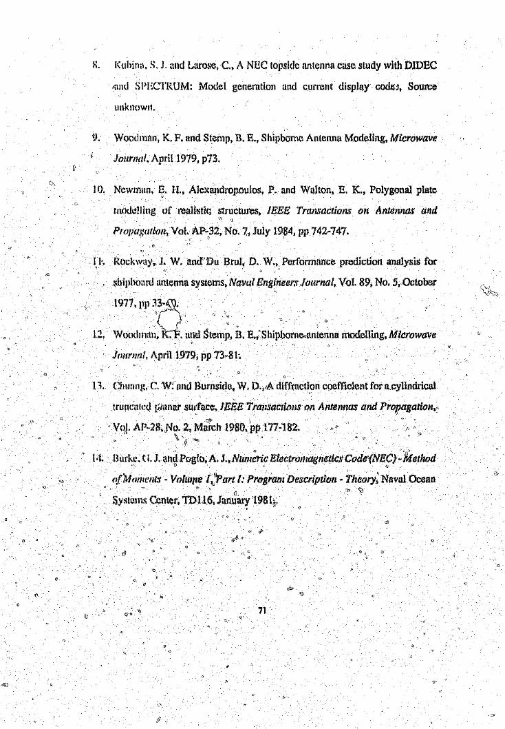
o
X. Kubin". S. J. and Larose, C.,A NEe topside antenna case study with DIDEe
Nand SPECTRUM: Model generation and current display code», Source
unknown.
9. Woodman, I<. F. and Sternp, B. E., Shipborne Antenna Modeling, Microwave
Journal, April 1979, p73.
10. Newman, E. Fl., Alexandropoulos, P. and Walton, E. K.. Polygonal plate
modelling of I'caHstic; structures, IEEE Transactions on Antennas and
Pmpagarloft,Vol. jt\P~32, No.7, July 1984, pp 742-747.
l l. Roc:kway,.l. W. and"Du Brul, D. W.) Performance prediction analysis for
lihiphoard antenna systems, Naval Engineers Journal, Vol. 89, No. 5"Oclooor
1977, pp 33·~.;..I ... ~"\.
'T \,\"., \.:: \)
12. Woodman, kj. ami Slemp, B. E., Shipbol'ncoantenna modelling, Microwave
Journal, April 1979, pp 73-8 L
13. Chu:lng, C. W: and Burnside, W. D.,I}\ diffractlon coefficient for a cylindrical
truncated pinnal' sUl'face.lE~E Transactions on Antennas and Propagation,
Vq!. AI'~28.N(). 2, M:fch 1980, pp 171':'182." """, '"
, 14, Burke. (i.J. i\1l(l.P(~glo.A. 1.,Num;ric El(!ctmmaglletlc.~ Code"(NEC) ~l't1ethod0' r. ' !,]
,; ,-,'. ,'", ',' (1 .,' ,', ' , "-",.:",,, ' '" ,~, "(~fl\ll(}fIl('nts - Volwtle [,,;Pal't I: Program DeSCl'l[JlUm ~Theory, Naval Ocean
Q
oSystems Center. TD116, JamlUl~19B!'!,
o
~j o
a
71
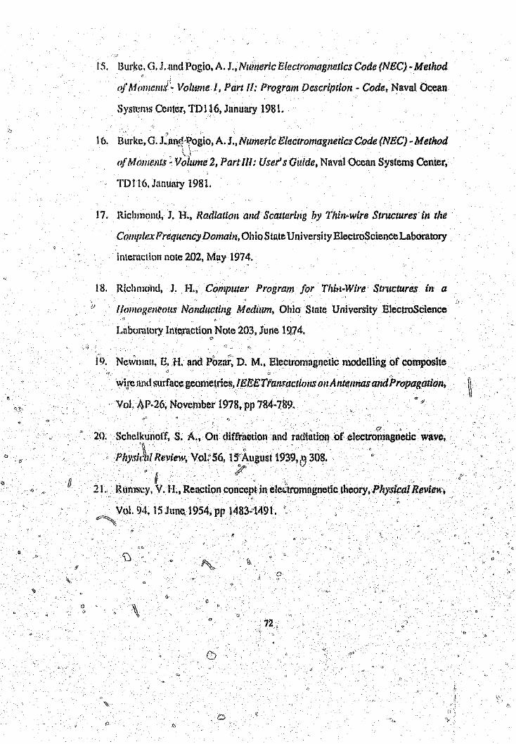
a
o
15. Burke. G. 1. and Pogio, A. J .• Numeric Blectromagnetics Code (NEC) ~Method
of MomelllS' v votume 1, Part J!: Program Description - Code, Naval Ocean
Systems Center, TD116, January 1981.
16. Burke,G.Lan1p,ogio, A. J., Numeric Electromagnetics Code (NEC) ~Method
of MOlJ1t!Jlts - Vdlwne 2, Part Ill: User's Guide, Naval Ocean Systems Center,
Tot 16,January 1981.
17. Richmond, J. H., Radiation and Scattering by Thin-wire Structures in the
Complex Frequency Domain, Ohio State Universi ty ElectroScience Laboratory
interaction note 202, May 1974.
18. Rlchn}(illd, J. H., Computer Program for ThiJL"Wire Structures in a
1l0l11O!F'll(!OUS NOllducting Medium, Ohio State University ElectroScience
Laboratory Interaction Note 203, june 1974.C\
19, Newnuur, H. H. and rozar, D. M,. Electromagnetic modelling of composite
wire and surface geometries.! EEE'Ttal1sactiolls on Antennas and Propagation, ',\\\
VoL i\P·26, November 1978, pp 784~789.
(J ,
20. Schelkunoff, S. A" On diffrhotion and ra(i'iutioq of electromagnetic wave,\\ ...,"PhYSi(lll Review, Vol:56, 15 August 1939, B 308.
II21. Rumsey, V . 1'1..Reaction concept in elCCll'Omngnetic theory t Physical Revtev:
Vol. 94, 15 June, 1954, pp 1483·'l,1}.91.~
f/
o(I o
72,
" 'I Ryall. C. E. and Peters, L., Evaluation of edge-diffracted fields including,
equavalcnt currents: for thg,caustic regions, IEftE 1'runscu;!lons o1JAntennas
und Propagation, Vol. AP~17,No.3, ,Ma.y 196~, pp 292-2.99.\1 '
Q .....~.... .,. ~
23 Kpuyou111Jlnn, R. G. and Pathak, ~f H., A Upifonr{Geomctric'al Theory .of
Diffraction for 1\ edge in It perfectly conducting surface, PrtJceedings of the
\\ IEEB, Vol.. 62, No: 11, November 1974, pp 1448 ..1461.<~,' .-'
24 Law. Pl'cs(on E., Shipboard Electr(}/~gll(Jtics, Norward, MA ;'Artech House.-\\
19R7.1/
25
AUll!lUlflS (uu[J'.mp(rgation, Vol. AP~35) No.9, Septemger1987, pp 1045~1048..~
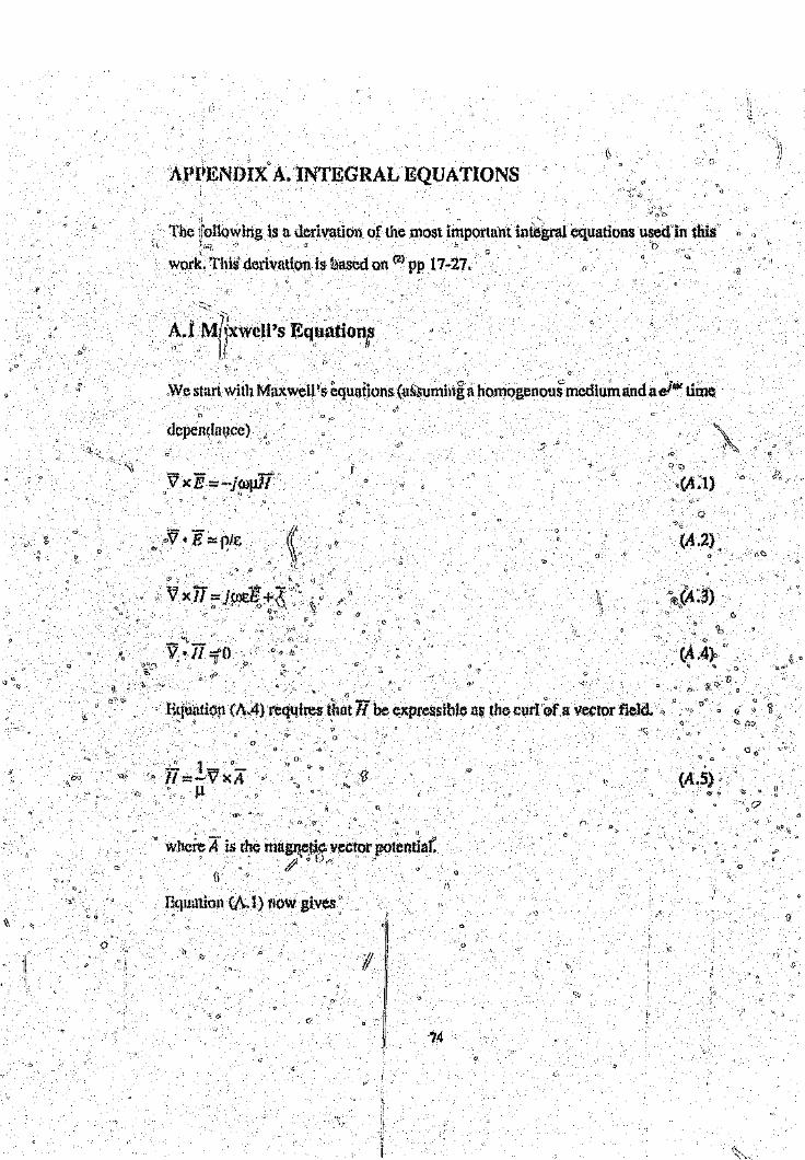
APPENOIX"A.INTEGRAL EQUATIONS
I _" . .._ . "-
The ifoHowhig is a derivation of the most important int~gral equations used in this
W01'k.Thisc derivation is based on (2) pp 17~27.
A.I .Ml~xweH'sEquation,s1(' "/)1.1
o l'
,Westart with Maxwell )5equuilons (u~~umhlg a homogenous medium and a eiCl)l time
dcpendH!Jcc)
Q
c" (A.2)
-- . ~- . - ....* -~v xlI ;;.i~1>eE0~» '~o o
v .n :.:fO., I)G.,)
c(1·4) s;
c
o
HquatiO!l (A.4)l'eql.dresthat f{ be,expressible n~ the curr~fa vector field. .o u
o''
o
(A.S)
Equation {I\.1) now gives(i
I)
74

(A.6)
where <!Jis ihe electric scalar potential.
(A.7)
VZ<!J+kZ~) :;::-pc, .
(A.8)
where k2;::::.(J)2qt and k"is called the propagation constant. The Lorentz" condition..
has now been imposed on $:,' ~:"
..;"
V •\~ :;::'Lj ())EWP (A.9)
.'Pm.'goog conductors (Where the current 7 atlU cttarge p reside on or very close to
c: the surface) Hehloiholtz's equl.ltions can be solved:
()
(AJO)
andCJ
(A.11)
whe2'c intcgrnticHlis .over the whole surface, S10fthe body,R ::: IF- ;:'1 is the dlstance
between the obscl;'atiO!1 point r (outside th~ surface of the conductor) and some,1
tI
75

point -;' on the surface of the conductor, J,r and P., are surface current and charge
dell :.; .....:and u and e are permeability nod permittivity for the medium outside the
CondUCLOr.
The law of conservation of charge also applies and this can be exprcsced as
(A .12)
or
v ·J ::::-:J'(l)p.$ S s (A .13)
where Vs denotes surface divergence.
The following boundary conditions apply between two diflerenlli1aterials:
(';=;(E· 1) .,:;{E·· 2»· x " -0·..". _f •. H:::: (A .14)
.... O(~1Y.1) -D· "(2K ..Pn· - ')=$ (A.15)
'0 (A .17)
where the sup<erscript(1) and (2) refer ro the fieIL!on either side of' the boundary and
76

A.2 The potential Integro-Differential Equation
The potential integro-differential equation is now given for a thin-wire.
If the wires are thin comsared to the wavelength and the distance between wire
junctions is sufficiently long compared to the radius, the following nssumptiuns are
valid:
(i) Current flow is ~)nrallelto the axis.
(ii) The axially-directed surface current density is unifonnly distributed around
the'tircumference.
(iii) The circumferential ~pmponent of 'the electric surface current is negligible,GJ . '. • o
(iv)
II ' " 59-../j 'I~ ~.
Axial electric surface current can be replaced by a line cllrrenl7.no{y>h~-::t~·n{g;
thewire axis:
(A.r8J
(v) Axltd surface charge can be replaced by a line chnrgt: q per, unit length('/ .
i;'
dlstrlbuted along the wire a~is: I, "
(A.19)
))/r
Equations (A. 10). (A.ll) and (A.l3) (:~J1now be simplifkd to:(?
(11.20)
77

CI
1i" . e-jkRtP(r):=- r q(l')--.... dl'\,' e wil'~ 41tR
- . dq(l)= J -1(1)
roll!
where lis the measure of!engMl alongthe wire.
(A .21)
(A .22)
The onlybo~:i\1:taryc0nditiollto be 81\ tisfied is the one concerninglhc axiii1componect
of the electric fJ~ldnnd this is from equurion (A.l4);
where f is a unit'vectorp.tndlefto the wire.c-
If we n6w assume that thp body will be illuminated by a plant! wave oK known,~ '. \) <;-Ih _ -,.I
amplitude"atiU pplads.\lion, the total electric field may be \I{).'ittcn :YlI:,- ,'._ -', - -- - - - - -- - - - ',- (}:;
(j
o(A.24), CI
from the body.
Taking equutiohs,,(A.6). (A.20) and (A,~l) into acc()ullnhc following equations(~: (\, t) ,', C,J -~'- I:f - n
follow:
d
78
c

(A.26)
11 e-jkll~.r 0:) :: -: . q (f')4 'R til'e WIT. 1t
(1\.27)
with the boundary condition (from equation (A.23»<)
(A.28)
For a perfect conducting material E(2):::: 0 whlle for a wh'e of finite conductiy~1Y it
~ay be calculated «(2)Chnprer 12) approximately us./.. . "<:..::-:::~
(A .?9)
where Z",is the Known. impedance per unit length of (he wires.!I
(i
By substituting equatk~lS (A..22), (A.25). (A.2""(.)and (1\.29) III (qmHioll (1\.28) the, c. ,
p..o.. teo n titl,~,:int.egrc:.)-tlif6e,r.•.entil.,i.l...•e.•c~."Ui..\.liO. n iSJ'Obftioeo for th...e, '.•..-urrenr;Jf)' Ii \\
o """;'i • i" ft,j .~ '1 ~ll(I') a ').e,7k11 . IZ)(I)-I. E (1)::;-) h"<l*f -/(1)+ J.__ . --dlwit~'\;.,S o.YLt ,dt' at 4nR
(A .30)
,17
" Toget Poeklingt8n Is hllegrttl eqp~ti()none substitutes etl~mtion (1\.9). into equation
o {A;(i) to give:
79

~A.31)
,~l
By going th~O~Jghthe same procedure of expressing this equa tion in tenus ofcunents,
and takjng the thin wirp approximation one arrl "es nt Pocklington' s in tegrufeq uatlon:i '
(A.32)
(p
wheret I' are uIlit vectors lying along the wire at the ebservation point! nIltI'sonrce
(polnt P respecdyely.
A.4 The Reaction Integral Equation (RIE)
Consider a geometry ofar.hitrary shaped scatterers in a homogeneous medium as
shownit're A.I. S is the syrfnceenclosing the scatterers and Ii is th~unit outward
nonn',;lto S .Note that S ni'ay be any closed surface such as so)id surfaces, wires and/; ~ .. ;.~)
" ,) ••c~inations. The ejUlt is suppressed, The sources (lit MJiJ genenHe the fields (J!;,"Ffj)
.•ffi'b spaeeand I~ field (E,H)ln thep~eS~t. "; ~'~:c.tI~",rs.Fro", SCl1"lkU~~fr."==--<~~e~eqllavalence theorem,(20) the fleld interior to thl~ surntte S (that IS in the
.'_- .' :. -.:, _-\.- _. ':-' -_ ,- _':,
conducting medium) wifl vanish without changingthe, exteti()rfiel~s if the ..surfuce (]
o current densities:
(A.33),)
o
HO
oand
{I
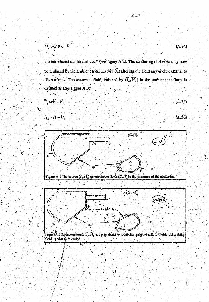
o
(A.34)
nrc i11lroduccd on the surface S (see figure A.2). The scattering obstacles may now
be rcplacc,d by the ambient medium with{;;t altering the field anywhere external to
the surfaces, The scattered field. irldiated by (ls;M.r) in the amblent medium, is
Ill~f$nedtIS (sec figJlreb.3):
71 ~H _·Ti.s· I (A.36)
f! ()
v
®t;1 0
()\)
I)
1/
81rj
.'/i I:
)
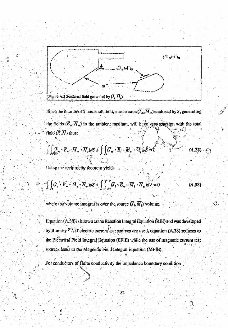
(I
Sillce the Interiorof S has n null field. u test source a:M".) enclosed by S Igenerating
(A.38)
whefe the''\\'olume integral is over the source t7h~) voluine,
Equation (A.'3~fJis known as the Reucilon Integral Equution (RIB) and was developed
hYJ{Ul11S'ty'{",l. If ~lcc[ric CtllTCllS~st sources .are used, equation (A.S8) reducesto
the El~btrki\1 Field !n~gral Equation (ErIE) whil;'the use of magnetic current test
sources ie,mfs to the Mngl1cdc r;ield Integral Equution (MFIE).o
a
For C()J11iuctors 9f~"..fll:.l~;e conductivity the impedallce boundary contlltion
"
" "» ', .•Oc'''
o
82o
is used. I~()rperfect conductivity Zs :::::M ~ :::::n.
i_")
\1
a
l ()r' 0
..t)
'':;'1
\\
C-
O
I]
83
(A.39)
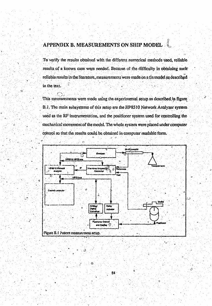
APPENIJIX It MEASUREMENTS ON SHIP MODEL
To verify the results obtained with the different numerical methods used, reliable
results of a known case were needed. Because of the difficulty in obtaining such'-z:
reliable results in the literature, measurerncntswere made on It lin model a~described
in the text.
This measurements were made using the experimental setup as described ;i~ figure,
13.1, The main subsystems of this setup are the HP851 0 Network Anulyzer system
used as the RF' instrumentation, and the posilioner system used for controlling the
mcchariicalrncvemcut of the model. The whole system were placed under computer
Cf?htrol so that the results could be obtained in compu ter readable form.
o
Figure B. t Puucrn mcasurcmcm setup.
84 \1
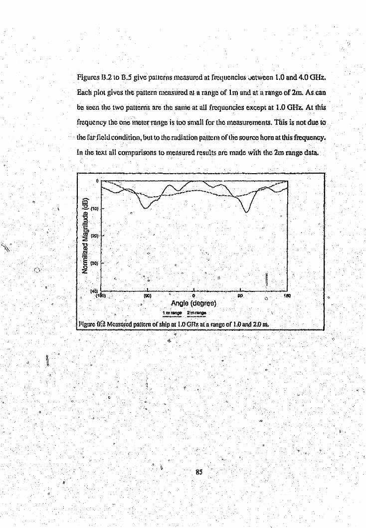
\\
Figures 13.2 to n.s give patterns measured at frequencies oetween 1.0 and 4.0 GHz.
Each plot gives the. pattern measured <\! a range of lrn and at a range of 2m. As can
be seen the two patterns are the same at all frequencies except at 1.0 GHz. At this
frequency the one meter range is too small for the measurements. This is not due to
the far field condi tion, but to the radiation pattern of the source horn at this frequency.
In the text all comparisons to measured results (iI'C made with the 2m range data.
OJ:g. (WI ~tbU.sc:;0)~ (20) •
'tl~.!::!
§ (30) •oZ
!I
liP 180Angle (degree)
1 In 'Mgl!) 2'"", range~ ------
t:igurc B~itMcusUr~A1paucrn of ship at 1.0 OlIr. nt a runge of 1.0 and 2.0 m,
85!f
c
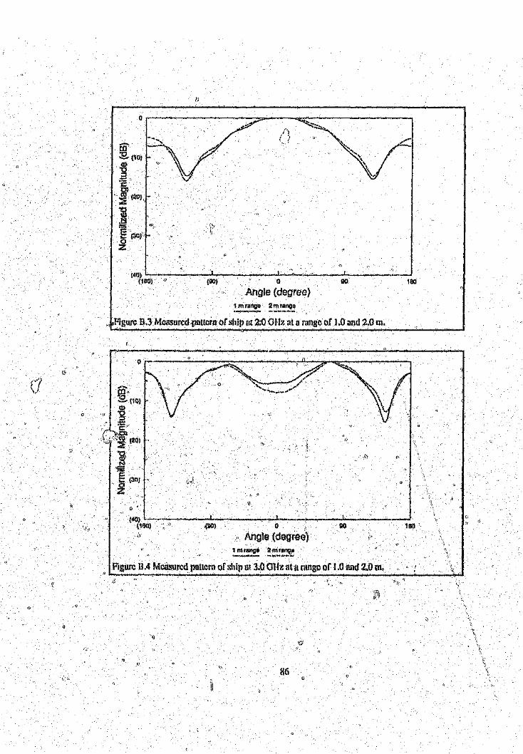
o
co:E,. ('0)O};gC0'1to (20). -::E ."tI~l).
:~g (:lof'~
~,,,,.L~~..........~__,__-...._(mOl a (OO) 0
I Angle (degree)1 mlMgo 2mrango
., ,Figure 11.3 MCllsurcd .pattern of ship at 2:0 .b~;;~~11runge of 1.0 ilnd 2.0 m,L-~'~ - ~ ~ __ ~ ~ ~~ __ ~ ~ ~
90
o --v~-__.0,., .,- .•••.. -- ~--:-; ---"'-'---- . ..,...._•.•. ~ .. ~//.' .. -'~, ~
....-.. .. . .. ,,- " ",.,' - - - ',", - -', ",.,/ ,._',', ": - - - - - - -~,CO:,, "," " - _,",' ........,.Jo... _~ .... - '\
~(1Q) \\.;g
=c:C;J'f""l
!.J"-='§ (30)
*o
(1 " ----~----~~----~~----~----~--~--~oAngle (degree)
11l()
(i(40)(VJO) ,(90) so
Figure n.4 Mctl"iu)'cd pattern of ship m 3.0 CHz at II range of 1.0 and 2.0 in.
86
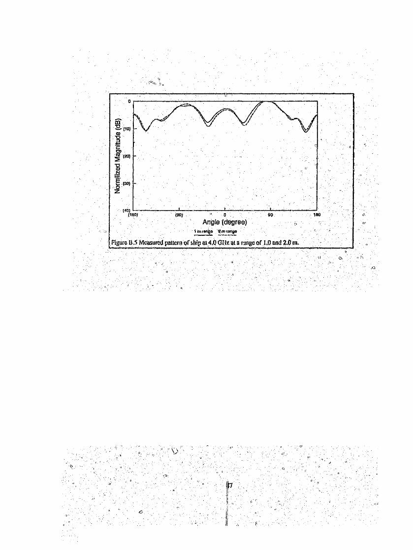
Or-
<>OJ:e. (10)(].)U:J:genrcl (;:!O)ZuQ)
.~'g (30) ,-oZ
,/.,-;..-,,~
J(40) L_."
(1!JO) (901 t) 90
Angle (degree)100
l11"III\~P ~~-,:,:g~Figure 115 Measured pattern of ship ut4,O om ul a range of 1.0 arrd 2.0 m.
c,
o
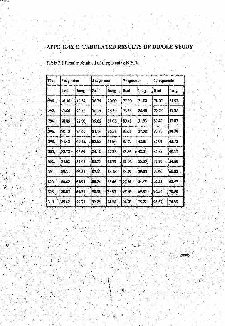
,APPE. !bIX C. TABULATED RESULTS OF DIPOLE STUDY
Table 2.1 Results obtained ofdipole using NEC2.
Frcq 3 segments 5 segments 7 segments 11 segments
Rent Imag Renl Imag Real Imag Real Imag
~90. 76.36 11.87 76,75 20.09 77.30 21.00 78.07 21.92
292. 77.60 23.48 78.19 25.59 78.85 26.48 79.75 27.38
294. 78.85 29.06 79.65 3t.()6 80.43 31.93 81.47 32.83
296. 80.12 34.60 81.14 36.52 82.05 37.38 83.22 38.28
298. HlAO 40.12 " 132.65 4L96 83.69 42.81 85.01 43.13,__....,
300. !{2.70 45.61 84.18 47.38 85.36 ")i 48.24 86.83 49.17,...302. 84.02 51.08 85.75 52.79 87.06 53.65 88,70 54.60
Q 304. 85.34 ,56.51 87.33 58.18 88.79 59.06i 90.60 60.03"
61.92\,
(]4.43306. 86.69 88.94 63.56 9Q,.56 92.55 6S.47,
(,'
'68.!)3 94.54Q 308•• SH.OS (,"1.31 <>0.58. 92.36 69.84 70.90
310. 81).42 72.77 92.25 74.28 94.20 75.22 96.57 76.33"
00
0(\ o
o
IT
88
to
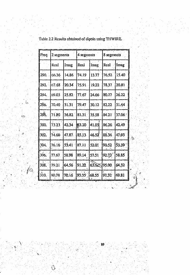
Table 2.2 Results obtained of dipole using TIIWIRE.
Freq 2 segments 4 segments 8 segments,
Real Imag Real Imag Real Imag
290, 66.36 14.86 74.19 13.77 76.52 15.40
292. m.68 20.34 75.91 19.22 78.37 20.81
294. 69.03 25.82 77.67 24.66 80.27 26.22
296. ,. 70.40 31.31 79.47 30.12 82.22 31.64
29i 71.80 36.82 81.31 35.58 84,21 37.06"~~.
I'
300. 73.2.3 42.34 W3.2() 41.0~1 86.26 42.49I
o 302. 74.6&' 47.87 85..13 46.5~! 88.36 47.93
(1 304. 76.16 53.41 87.1 1 52.01 90.52 53.39.., " "0
..,
306. 77.67 58.98 89.14 57.51 92.?p 58.85, ~"'''o;
308. 79.21 64.56 91.22 63"t1:"';,c 95.00 .64.32J ..... <.,.'
o~Yo") o
310. xn.7S 70.16 93.35 68.55 97.32 69.81-=.:. , n
89
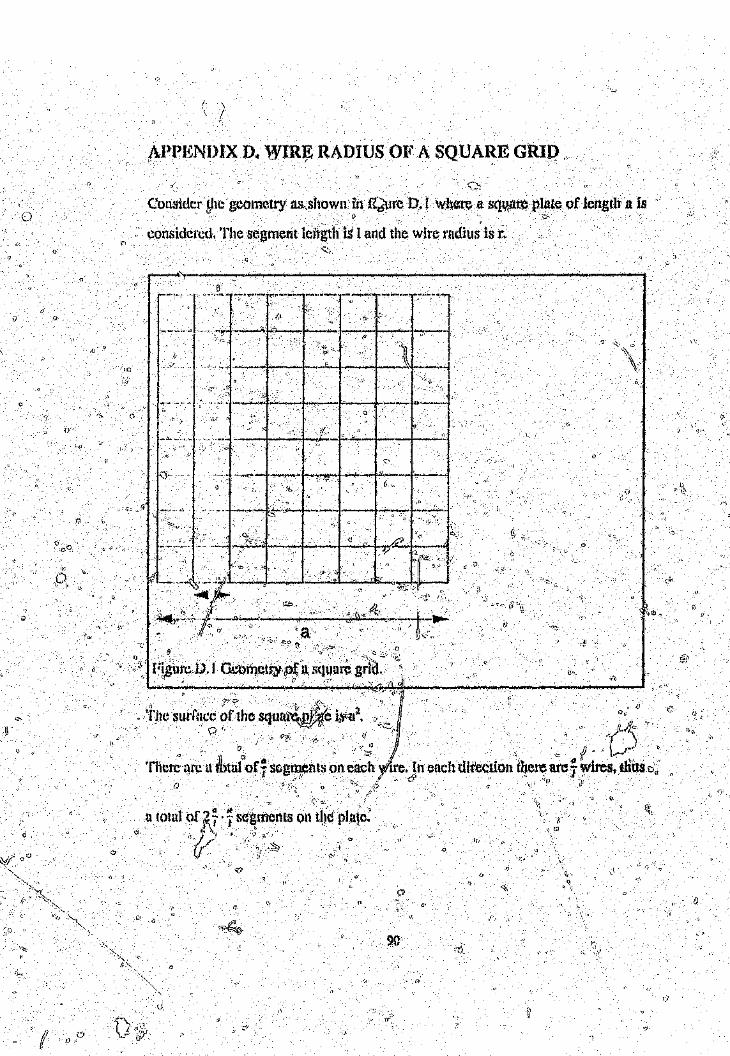
APPENDIX D. 'YIRJi: RADiUS OF A SQUARE GRID
Consider ,t;hc'geometry as.shown. in f~;;tlreD, f· wlie-r~a sqWtre plate of length a is
considered, The segment ICligth is 1and the wire radius is r.
'--'-'_......--_"_,/......__ "''";" . 7\';0::1-- -1} ,:; ••••• :, ••••• I''I'he Stll'f\ICC ~)flheSqll~:.'~Aiei;)"i, ,j',:::.1 0,
u," 0 .j ,_ /), "Ther~ arc it Jbta{'orT sogn~entson each yA~e.~~neach direction 'tryere areTwires, thus D"
~~ 0,,',")
o
90
()

The/area of a segment is 2nrl. 1/
As the 101aJ:are.ofthe wires must be equul;-tp lWO times the area of the plate:\.·l· t._·_./~
2 1.2...0 a 2· z7C1' '. - .-;::: a. I I
()r-t
r=-I,,,,O.159121t
9)

APPENDIX E. WIRE RADIUS OF A TRIANGULAR GRID
Consider tile geometry I1S shown in figure E.1 where a triangular plate with all sides
equul to H is considered. The segment length is I and the wire radius is r,
\,\
7\\\\,\
o-~-------.,....., ------...:,...----.---~--_...-.....\,
I) TfK~surface of the triangular plate i\;~~3a2." I',
'\\I'\\IIII . \
Thl~I'Carc n total (';r37 wires on the ~l~ate.l'henumber of segments per wirivarics11. ,; ,,' " .. It 'j}>' . \"~)\1 "j
It, \\I, I I[ '" 'I',· '1 . l' ,0 l rQ' "f)n 3(n "Iz f Irom l~~l\ iere are tHIS a totn Of;;:( ',.+,} ,- "":;- -, 1 :segments on t ie pate.
)I , ., it; , . " " Jll) _ l! (\ !O '\-,
itIi
\~

The area or a segment is 2nrl.
As the total area of the.wires must be equal to two times the urea. of the plate:
13r =-1 ",0.09167t
)'"/' i
\1 93

..

Author: Botha Louis.Name of thesis: The Prediction Of The Interaction Between Shipboard Antennas And Their Environment.
PUBLISHER:University of the Witwatersrand, Johannesburg©2015
LEGALNOTICES:
Copyright Notice: All materials on the Un ive rs ity of th e Witwa te rs ra nd, J0 han nesb u rg Li b ra ry websiteare protected by South African copyright law and may not be distributed, transmitted, displayed or otherwise publishedin any format, without the prior written permission of the copyright owner.
Disclaimer and Terms of Use: Provided that you maintain all copyright and other notices contained therein, youmay download material (one machine readable copy and one print copy per page)for your personal and/oreducational non-commercial use only.
The University of the Witwatersrand, Johannesburg, is not responsible for any errors or omissions and excludes anyand all liability for any errors in or omissions from the information on the Library website.