THE PRODUCTION IMPACT OF “CASH-FOR-CLUNKERS”: IMPLICATIONS FOR STABILIZATION POLICY

THE PRODUCTION IMPACT OF ‘‘CASH-FOR-CLUNKERS’’:IMPLICATIONS FOR STABILIZATION POLICY

ADAM COPELAND and JAMES KAHN∗

Stabilization policies frequently aim to boost spending as a means to increase grossdomestic product. Spending does not necessarily translate into production, however,especially when inventories are involved. We look at the “cash-for-clunkers” programthat helped finance the purchase of nearly 700,000 vehicles in 2009. An analysis ofauto sales and production movements reveals that the program did prompt a largespike in sales. But the program had only a modest and fleeting impact on production, asinventories buffered the movements in sales. These findings suggest caution in judgingthe efficacy of such policies by their impact on spending alone. (JEL E23, E65, L62)

During July and August of 2009, Ameri-cans purchased nearly 700,000 new automo-biles or light trucks under the government’s“cash-for-clunkers” program—officially the CarAllowance Rebate System, or CARS. Under theterms of the purchase, qualified buyers tradedin their old vehicles to receive a rebate onthe price of a new vehicle; the amount of therebate—either $3,500 or $4,500—depended onboth the model that was traded in and the modelthat was acquired. The direct cost to taxpay-ers of subsidizing these purchases was roughly$2.8 billion.

The program had two primary goals: toreduce energy consumption and pollution byinducing consumers to replace their old gas-guzzlers with newer, fuel-efficient models, andto serve as a stimulus for the troubled auto-mobile industry and the U.S. economy as awhole. In this article, we take a close look atthe second objective, exploring how the CARSprogram affected sales and, more important, pro-duction in the automobile industry.1 Drawing on

*The views expressed in this article are those of theauthors and do not necessarily reflect the position of theFederal Reserve Bank of New York or the Federal ReserveSystem.Copeland: Research and Statistics Group, Federal Reserve

Bank of New York, New York, NY. Phone 1-212-740-7490, Fax 1-212-740-8363, E-mail [email protected]

Kahn: Henry and Bertha Kressel Professor, Departmentof Economics, Yeshiva University, New York, NY.Phone 1-212-960-5400, Fax 1-212-960-0846, [email protected]

1. An assessment of the returns on the $2.8 billiongovernment expenditure would have to include a valuation

our findings, we then propose an answer to themore difficult question of the program’s impacton U.S. gross domestic product (GDP).2

In line with other recent studies, our analysisshows that the CARS program had only a transi-tory cumulative effect on sales. We estimate aninitial impact of about 450,000 additional auto-mobile sales, but these were essentially shiftedfrom the periods before and (especially) after theprogram. We calculate that by January 2010, thecumulative effect of the CARS program on autosales was essentially zero.3

of the energy efficiency gains achieved through the program.However, this is an issue we do not address in the article.

2. Li et al. (2010) and Mian and Sufi (2010) examineonly the sales impact of the CARS program. Abrams andParsons (2009) study the welfare effects of the program,weighing the benefits to consumers who received subsidiesfrom the CARS program against the costs to taxpayers andtaking into account the environmental gains of cleaner air.Their back-of-the-envelope calculations show that the costsexceeded the benefits by approximately $2,000 per vehicle.

3. In dollar terms, our estimates suggest that almost$4 billion in nominal sales were moved up from the fourthquarter to the third quarter of 2009.

ABBREVIATIONS

CARS: Car Allowance Rebate SystemCEA: Council of Economic AdvisersCUV: Crossover Utility VehiclesDID: Difference-in-DifferencesDOT: Department of TransportationECT: Error Correction TermGDP: Gross Domestic ProductGVWR: Gross Vehicle Weight RatingSUV: Sport Utility VehiclesVEC: Vector Error Correction

1

Economic Inquiry(ISSN 0095-2583)

doi:10.1111/j.1465-7295.2011.00443.x© 2012 Western Economic Association International

2 ECONOMIC INQUIRY

More important for our purposes, however, isthe program’s effect on automobile production.While most studies of CARS have focused onsales, we argue that the program’s success as astimulus to the economy hinges on its impact onproduction. Production increases are more likelyto translate into higher GDP and employment,GDP being fundamentally a measure of produc-tion. Sales clearly rose at the outset, but giventhat the industry can simply let inventory stocksabsorb the increase in sales, higher sales alonedo not imply higher GDP or employment.4

Overall, we find that the program had a verymodest and short-lived effect on production.Production was about 200,000 units higher dur-ing the program (in comparison to the 450,000increase in sales). Sales from September 2009 toJanuary 2010 were correspondingly lower thanthey would have been in the absence of CARS,which allowed producers to have lower pro-duction while still replenishing their inventorystocks. Thus on a quarterly basis we estimatethat the CARS program shifted production byaround 100,000 units from 2009Q4 and 2010Q1to 2009Q3.

These calculations suggest that the programhad a negligible direct effect on GDP, shiftingless than roughly $2 billion (or less than one-tenth of 1% of GDP) into 2009Q3 from the sub-sequent two quarters. This contrasts starkly witha study released by the Department of Trans-portation (DOT) in the immediate aftermath ofthe program, which concluded that CARS hadgiven a substantial boost to both GDP andemployment. In the final section of the arti-cle, we discuss why our conclusions differ fromthose of the DOT study.

Our findings raise broader questions, beyondjust this particular program, about the efficacyof efforts to stimulate short-term spending. Itis clearly a mistake to gauge their impact byjust looking at the spending they induce, withoutlooking at the supply side. It is reasonable toexpect that producers will use other marginsthan production and employment to respondto temporary movements in sales, so the onlyquestion is quantitative: How large is the gapbetween the sales and production impact? Wefind it to be large in the case of “Cash-for-Clunkers.”

In what follows, we will lay out the eco-nomics behind our analysis by examining how

4. Even production increases might not result in higherGDP if resources are diverted from other industries. This isperhaps less likely to be an issue during a recession.

rebates and other transitory price changes affectconsumer purchases and manufacturers’ inven-tory decisions. We then provide some back-ground on the Cash-for-Clunkers program inSection II. Sections III and IV provide our anal-ysis of the impact of the program, and Section Vconcludes.

I. DURABLE GOODS AND INVENTORIES

A. Consumers

The consumer response to temporary pricechanges—including rebates and other subsi-dies—differs dramatically for durable and non-durable goods. Automobiles are a type ofdurable good, that is, a good that can be used or“consumed” over a number of years. Because adurable good can be stored, a temporary declinein its price will prompt consumers to “stockup.” By contrast, a temporary drop in the priceof a nondurable good—a good, such as milkor lawn-mowing services, that is quickly con-sumed through use and cannot be stored—willnot cause people to stock up.

Moreover, in the case of durable goods,consumers have considerable latitude in timinga purchase. Someone planning to replace a“clunker” can easily shift the timing by a fewmonths. So it is natural not only to expect a largesales response to a temporary subsidy for anydurable good but also to expect that much of thatresponse will be offset by lower sales before orafter the subsidy period, as consumers defer ormove up their purchases to take advantage of thesubsidy.5 Thus the cumulative impact on sales(and hence, production) is likely to be modest,if not zero, over a longer time frame. The onlyissue is how long it takes for the impact todissipate: Do consumers shift their purchases bya few weeks, a few months, or longer?

B. Producers

For automobile producers, the key decisionsare when and how much to produce in responseto a temporary subsidy. Most automobiles aresold from inventories, not specially ordered.Dealers on average maintain inventories equiv-alent to approximately two and a half months’

5. Erdem, Imai, and Keane (2003), Gowrisankaran andRysman (2010), and Hendel and Nevo (2006) demonstratethe importance of accounting for the timing of consumerpurchases when comparing the effects of temporary andpermanent price changes in durable goods.

COPELAND & KAHN: CASH-FOR-CLUNKERS AND PRODUCTION 3

worth of sales.6 Deviations from the averagemay occur for a variety of reasons—seasonalfactors, an unexpected blip in sales, or changesin production or inventory holding costs—butthey rarely persist. A large positive surprise insales will cause inventories to decline for a timeuntil they can be replenished by additional pro-duction. An anticipated jump in sales, if believedto be temporary, will also result in a declinein inventories, largely because producers gen-erally find it costly to change production by alarge amount in either direction.7 And if thatjump is viewed as, in effect, borrowed fromfuture sales, no additional production is nec-essary to replenish inventories; the subsequentdrop in sales will restore stock levels if produc-tion remains constant. Given this reluctance toboost or cut production significantly, an increasein sales that is accompanied by an increase ininventories is a sign that producers view thesales upturn as likely to persist. But if the jumpin sales is viewed as just coming at the expenseof future sales, it makes sense for firms to letinventory movements accommodate much of thesales movement rather than change productionby a substantial amount.

Automobile producers and dealers thus havea number of options in responding to programslike CARS. If they have advance notice of theprogram, manufacturers can shift production for-ward to build up inventories, and then let thespike in sales following the launch of the pro-gram reduce inventories to normal levels. At theother extreme, they can leave their productionplans unchanged, let inventories absorb the spikein sales, and then wait for inventories to recoverwhen sales drop after the program expires. Thefirst approach emphasizes the desire to avoid anystockouts, so as to maximize the sales from theprogram; the second emphasizes the firm’s goalof minimizing its costs by smoothing productionand letting inventories serve as a buffer.8

In actual practice, producers most likelyadopt some combination of the two responses,

6. One explanation for the large inventory holdings isthat dealers wish to avoid “stocking out,” that is, not havingthe models on hand that buyers want. See, for example, Bilsand Kahn (2000) and Kahn (1987, 1992).

7. Bresnahan and Ramey (1994) analyze the differentways that automobile manufacturers adjust production andthe respective costs.

8. Copeland and Hall (2011) offer a detailed empiricalanalysis of automakers’ response to temporary demandshocks. They find that shocks are almost entirely absorbedthrough adjustments in sales and production rather thanadjustments in prices.

because they care about avoiding stockouts andsmoothing production. The relative importancethat they assign to these motives will dependin part on the costs of shifting production for-ward to meet increased demand—for example,paying workers overtime, running second shifts,and coping with bottlenecks in supplies. It willalso depend on the amount of profit that wouldbe lost in the event of a stockout, which in turndepends on the size of the price-cost markup onthe automobiles. Since the CARS program likelyboosted these markups, we would expect at leastsome increase in production to avoid stockouts.

C. Seasonality

An additional complication affecting the pro-duction of automobiles is seasonality. U.S.automobile manufacturers typically shut downproduction for a period of weeks in the summerto retool plants for the next model year. Duringthis time, they draw down inventories of the pre-vious year’s model and then begin to accumulateinventories of the new model after productionstarts up again. Manufacturers also shut downproduction during the Christmas–New Year’speriod for a week to 10 days. These large andvariable seasonal movements must be taken intoaccount in analyzing industry data, especiallythe numbers in July and August—all the moreso because in 2009 the CARS program was ineffect during precisely those 2 months.

Despite these complications, the CARS pro-gram represents a unique opportunity to studythe behavior of both consumers and produc-ers. Particularly advantageous for our analysisis the fact that only some vehicle models wereeligible for the rebate.9 While the existence ofa subsidy may have induced some consumersto buy an eligible model when they otherwisewould have chosen to buy an ineligible model,we nonetheless are able to use the data on theproduction and sales of ineligible models as a“control group” to help gauge the impact of theprogram.

II. A TIMELINE OF THE CARS ACT

Early notice of the cash-for-clunkers pro-gram appeared in a December 2008 article in

9. The availability and size of the rebate depended onthe extent to which the purchaser traded up in fuel efficiency.Some models were not eligible at all, while higher-fuel-efficiency models increased the number of buyers who couldmeet the eligibility requirements.

4 ECONOMIC INQUIRY

TABLE 1Overview of the Link Between Cash-for-Clunkers Rebates and mpg

New Vehicle

Trade-in Vehicle TypeMinimum

mpgDifference BetweenNew and Trade In

RebateDollars

Automobile Automobile 22 mpg 4–9 mpg 3,500≥10 mpg 4,500

Category 1 Truck 18 mpg 2–4 mpg 3,500≥5 mpg 4,500

Category 1 and 2 Truck Automobile 22 mpg 4–9 mpg 3,500≥10 mpg 4,500

Category 1 Truck 18 mpg 2–4 mpg 3,500≥5 mpg 4,500

Category 2 Truck Category 2 Truck 15 mpg 1 mpg 3,500≥2 mpg 4,500

Category 3 Truck Category 2 Truck 15 mpg n.a. 3,500Category 3 Truck n.a. n.a. 3,500

Notes: Automobiles and Category 1 and 2 trucks being traded in must have mpg ≤18.Category 1 Truck: SUVs with a gross vehicle weight rating (GVWR) of less than 8,500 pounds, pickups with a GVWR

of less than 8,500 pounds and a wheelbase of 115 inches or less, and passenger vans and cargo vans with a GVWR of lessthan 8,500 pounds and wheelbase of 124 inches or less.

Category 2 Truck: Pickups with a GVWR of 8,500 pounds or less and a wheelbase greater than 115 inches and passengervans and cargo vans with a GVWR of 8,500 pounds or less and a wheelbase greater than 124 inches.

Category 3 Truck: Very large vans, SUVs, and pickup (cargo bed of 72 inches or more) trucks with GVWR 8,500–10,000pounds.

the San Diego Union-Tribune reporting that theNational Automobile Dealers Association waslobbying the incoming Obama administrationto include the program in the economic stim-ulus bill.10 Cash-for-clunkers quickly became apart of the economic stimulus package. In lateMarch 2009, the Obama administration endorsedthe idea of a trade-in program for automobilesand, on June 9, the House of Representativespassed a cash-for-clunkers program.11 The Sen-ate quickly followed and, on June 24, the CARSAct of 2009 was signed into law.12 Congressallocated $1 billion to fund the program, andnew car purchases and leases on and after July 1were made eligible for rebates.13 Because of

10. James Oliphant and Richard Simon, “Line Formingfor Slice of Stimulus Pie,” San Diego Union-Tribune,December 15, 2008.

11. Bryan Walsh, “Cash for Clunkers: A Green Deal toHelp Detroit?” Time.com, April 15, 2009; Jennifer Liberto,“House OKs $4 Billion ‘Clunker’ Bill,” CNNMoney.com,June 10, 2009.

12. The CARS acronym was applied to both the legis-lation establishing the program and the program itself, butthe acronym was interpreted differently in the two cases.While the title of the program was “Car Allowance RebateSystem,” the “CARS Act of 2009” was short for “ConsumerAssistance to Recycle and Save Act of 2009.”

13. Catherine Clifford, “‘Cash for Clunkers’ ComingSoon,” CNNMoney.com, June 24, 2009.

the popularity of the CARS program, an addi-tional $2 billion was allotted to the program onAugust 7.14 Even with this extra allotment, thecash-for-clunkers program ran out of funds andended on August 24. Overall, more than 677,000vehicles received cash-for-clunkers financing,and roughly $2.8 billion was disbursed throughthe program.15

The size of the cash-for-clunkers rebate waslinked to the difference in miles per gallonbetween the vehicle traded in and the new vehi-cle purchased (Table 1).16 The set of new vehi-cles eligible for financing through CARS wasquite broad, and included larger vehicles suchas sport utility vehicles (SUVs), vans, and pick-ups. However, a quick scan of the vehicle typespurchased under the program (Table 2) revealsthat the program mostly helped to finance thepurchase of small cars and crossover utility vehi-cles (CUVs). Cash-for-clunkers rebates were

14. Sharon Silke, “Obama Signs $2B Cash for ClunkersExtension,” ABCnews.com, August 6, 2009.

15. “Secretary LaHood Touts Success of Cash forClunkers; Responds to Reports by DOT Inspector General,GAO,” Department of Transportation press release, April29, 2010.

16. Visit http://www.cars.gov for a full description ofthe CARS program and its eligibility requirements. For alist of the names of vehicles that were eligible for CARSfinancing, see http://www.edmunds.com.


TABLE 2Cash-for-Clunkers Financed Sales by Vehicle Type

CFC Sales

July(units)

August(units)

July + August(units)

CFC Sales / EligibleSales (%)

CFC Sales / TotalSales (%)

Small cars 75, 508 171,920 247,428 45.1 45.1Middle cars 43, 883 97,356 141,239 27.4 27.0Large cars 292 840 1,132 4.5 3.0Luxury cars 1, 291 4,708 5,999 8.1 4.2CUV 54, 702 111,456 166,158 36.6 35.1SUV 5, 913 17,742 23,655 19.8 16.3Pickup 22, 330 49,133 71,463 25.1 25.1Van 4, 826 11,483 16,309 19.2 16.4Total 208, 745 464,638 673,383 32.0 29.9

Note: “CFC sales” stands for sales that received a cash-for-clunkers rebate, “eligible sales” stands for sales of cars eligiblefor a rebate. There were 677,081 CFC sales in the original data. After cleaning the data (e.g., dropping observations with“unlisted” model names) there were 673,383 CFC sales.

received for 45% of all small car sales and 35%of all CUV sales in July and August. In contrast,large cars and luxury cars received little directbenefit from the CARS program.

With 70% of all cash-for-clunkers rebatesgoing to sales in August, the program clearlyhad a much larger impact in August than inJuly. The injection of $2 billion in additionalfunding on August 7 no doubt helps account forthis difference, as does the fact that the CARSprogram eligibility criteria for a new vehiclepurchase were not finalized until July 24. Hence,consumers may have delayed their purchasedecisions in order to be sure that they qualifiedfor the cash-for-clunkers rebate.

The CARS program was used to finance salesof “old” 2009 model vehicles more often than“new” 2010 model ones. More than 75% of allsales receiving a cash-for-clunkers rebate were2009 model vehicles. Because most automobilemanufacturers switched from producing 2009models to 2010 models over the summer of2009, the vast majority of 2009 model salesin July and August came from inventories. Incontrast, because inventories of 2010 vehicleswere quite low in the late summer months,most of the new models financed through thecash-for-clunkers program came from currentproduction.

III. IMPACT OF THE CARS PROGRAM:PRODUCTION, INVENTORY, AND SALES DATA

As a first step in analyzing the effects of theCARS program, we look at aggregate data on

sales, production, and inventories for the U.S.automobile market in the period from January2007 through February 2010. We then breakout the data into vehicles that were eligible forfinancing under the CARS program and vehi-cles that were not. Eligible models accounted forroughly 75% of sales before the start of the pro-gram.17 More details about the data constructionare available in Appendix A.

The U.S. recession that began in December2007 hit automobile sales particularly hard.Sales declined sharply from the beginning of2008 and bottomed out in the first half of2009 (Figure 1).18 During the lows reached inearly 2009, both Chrysler and General Motorsdeclared bankruptcy.19 The launch of the CARSprogram reversed this downturn for a time,producing a temporary burst in sales in July andAugust of 2009 (Figure 1, shaded area).

The decline in automobile sales during therecession led to a large buildup in inventoriesfrom mid-2008 through early 2009. Economistsoften measure inventory holdings by looking at

17. We caution that eligibility had a quantitative as wellas a qualitative component: Because the program required adiscrete improvement in fuel efficiency, some models wouldbe eligible for only a small fraction of buyers.

18. Unless indicated otherwise, all data have beenseasonally adjusted using month dummy variables in a log-linear regression. The Bureau of Economic Analysis onlyprovides seasonally adjusted data for aggregates, but ouranalysis requires data on eligible and ineligible models.

19. We do not explicitly take into account any impactfrom the bankruptcies of Chrysler and General Motors,because these took place before the launch of the CARSprogram.

6 ECONOMIC INQUIRY

FIGURE 1U.S. Automobiles (Seasonally Adjusted)

Note: The shaded area indicates the months when theCARS program was in effect.

Source: Ward’s Communications.

FIGURE 2Months’ Supply of U.S. Automobiles

(Seasonally Adjusted)


Source: Ward’s Communications; authors’ calculations.

the ratio of inventory to sales, or “months’ sup-ply.” This statistic captures how many monthsof sales—at the current rate of sales —couldbe sold out of the current stock of inventories.Figure 2 shows that at their height in the lastquarter of 2008, automobile inventories wereequivalent to 3.8 months of sales. However,months’ supply declined substantially thereafter,essentially returning to its normal level of about2.5 months by June 2009. Given the low level ofsales, the drop in months’ supply had to reflect aparticularly large decline in inventories. Indeed,inventories fell from a pre-recession peak ofabout 3.3 million vehicles to less than 2 million.With the implementation of the CARS program,inventories plunged further, and months’ supply

FIGURE 3U.S. Automobile Production


Source: Ward’s Communications; authors’ calculations.

fell below 1.5 months, its lowest level in ourdata for the 1994–2010 period.

The large decline in inventories during theCARS program indicates that production, to-gether with net imports,20 remained far belowsales. Production did increase at the beginningof the program, however (Figure 3). The season-ally adjusted data show a production upswingin July 2009; moreover, actual, or unadjusted,output did not experience the usual 40% Julydecline (evident in 2007 and 2008) associatedwith the model changeover period but insteadrose 1%. Production then remained close toJuly’s level through February 2010, suggestingthat automakers expected the demand for auto-mobiles to remain firmer than in the first half of2009.

A breakout of the inventory data into vehiclesthat were eligible for CARS financing and vehi-cles that were not reveals that the August dropin the months’ supply of vehicles took placeentirely in the “eligible” category (Figure 4).This measure fell because sales of eligible vehi-cles increased while inventories of these samevehicles decreased. Recall that 2009 model vehi-cles made up fully three-fourths of CARS-financed sales. Since production of these “old”model vehicles ended in the summer of 2009,the data suggest that inventory reductions ratherthan additional production accounted for a sub-stantial portion of the increased sales in July andAugust of 2009.

20. See Appendix A for a discussion of the importanceof controlling for net imports when analyzing the CARSprogram’s effects on production.


FIGURE 4Months’ Supply of U.S. Automobiles, Eligible

and Ineligible Vehicles

Note: “Eligible vehicles” are those that qualified for arebate under the CARS program; “ineligible vehicles” didnot meet the criteria for a rebate. The shaded area indicatesthe months when the CARS program was in effect.

Source: Ward’s Communications; https://www.edmunds.com; authors’ calculations.

We can see more direct evidence in theproduction and sales patterns for eligible andineligible vehicles. We do a simple difference-in-differences (DID) estimation, comparing thechanges in sales and production of eligibleversus ineligible models before, during, andafter the program. In contrast to the standardbefore and after treatment categorization, weallow for the treatment to have a dynamic impactover time. Specifically, let se

t and snet denote

sales of eligible (e) and non-eligible (ne) modelsin period t , and let ye

t and ynet similarly denote

production. Consider the following model foreach variable:

ln(xjt ) = aj + bt + γj t +

t0+T∑

s=t0−1

cjs D

js=t + ε

jt

(1)

for type j = e or ne, and date t , where the “treat-ment” begins at t0, D

js=t is a dummy variable for

being at date t and in group j , and x refers toone of the four variables above. We allow forsome impact of the program in June becauseof the congressional action that began thatmonth. This specification allows for differentlevels and trends for eligible and ineligible vehi-cles, as well as common time effects. We esti-mate parameters for both production and salesusing least squares with ln(se

t ) − ln(snet ) and

ln(yet ) − ln(yne

t ) as dependent variables, whicheliminates the pure time effects. That is, we

estimate

ln(set ) − ln(sne

t ) = ae − ane + (γe − γne)t(2)

+t0+T∑

s=t0−1

(ces − cne

s )Ds=t

+ εet − εne

t .

We use monthly data from January 2004 toFebruary 2010, where t0 is equal to July 2009,and include a correction for serial correlation ofthe residual.

Equation (2) makes clear that the coefficientson the {Ds=t } correspond to the net impact ofthe program in each of the periods. As discussedlater in the article, the impact of the program onsales of ineligible vehicles could have been pos-itive or negative. For now, our baseline assump-tion is that it was zero. The estimates look at theperiod-by-period differences between sales (orproduction) of eligible versus ineligible modelsfor an estimate of the impact of the program,and are shown in Figure 5.21 The estimated salesimpact is both striking and plausible: signifi-cantly higher sales during the 2 months of theprogram, followed by a “payback” of low salesover the subsequent 6 months that more or lesscompletely offset the gains in July and August.But more striking are the production results: Forall months the effects are much smaller and atbest marginally significant. One can read intothe June figure a modest uptick in productionin anticipation of the program, followed by off-setting cuts in the months after the program, butfew of the effects are statistically significant, andin any case the cumulative impact is zero byJanuary 2010.

The very modest production impact depictedin Figure 5 is not completely surprising giventhe inventory behavior depicted in Figure 4.Clearly a portion of the sales were met bydrawing down inventories. The DID resultssuggest that portion was very high.

The difference between the sales and pro-duction responses is particularly noteworthy.In effect, this is a “differences-in-differences-in-differences” result: Any concern about themethodology (that the program affected bothgroups) would also have to explain why theeffects are so different on production versussales. If these findings are conclusive, they

21. In Appendix B, we report the detailed regressionresults.

8 ECONOMIC INQUIRY

FIGURE 5DID Results of the Impact of Cash-for-Clunkers on Sales and Production

-.3

-.2

-.1

.0

.1

.2

.3

.4

.5

Jun

09

Jul 0

9

Aug 0

9

Sep 0

9

Oct 09

Nov 0

9

Dec 0

9

Jan

10

Feb 1

0

Sales

-.3

-.2

-.1

.0

.1

.2

.3

.4

.5

Jun

09

Jul 0

9

Aug 0

9

Sep 0

9

Oct 09

Nov 0

9

Dec 0

9

Jan

10

Feb 1

0

Production

Note: Columns represent estimated coefficients and dotted lines are the two standard deviation interval. The units of thecoefficients are logarithmic deviations.


would suggest that the increases in automobileproduction beginning in the second half of 2009were not primarily due to the CARS program,but instead owed much to the general firmingof automobile sales that was taking place asthe recession was ending. The next section sup-plements these findings with a more structuralapproach.

IV. AN EMPIRICAL MODEL OF PRODUCTIONAND INVENTORY BEHAVIOR

In this section, we undertake a more ambi-tious effort to quantify the impact of CARS. Westart with a forecasting model based on auto-mobile sales and production data from January1994 through June 2009 as well as on con-temporaneous indicators of economic conditionsduring and after the CARS program. From this,we obtain an estimate of what sales would havebeen from July 2009 to February 2010 in theabsence of the program.

We then examine alternative assumptionsabout inventory behavior to obtain estimatesof what production would have been. The dif-ference between actual automobile sales andproduction and these counterfactuals providesestimates of the net impact of the program.Overall, the stronger the sales and productionmeasures in our counterfactuals, the smaller theimpact of the program will appear to be.

The first counterfactual scenario (Scenario 1)relies solely on the results of a vector errorcorrection (VEC) model. We use a VEC modelto reflect the long-term relationship betweeninventory levels and production. Our model hastwo endogenous variables (all variables are inlogarithms): U.S. sales of vehicles eligible forCARS at date t (se

t ); and U.S. inventories of eli-gible vehicles (ie

t ). We also include non-motor-vehicle industrial production (zt ) and sales ofineligible vehicles (sne

t ) as exogenous variables,current and lagged. Both of these represent vari-ables that are intended to help with the dif-ficult question of what would have happenedto the endogenous variables in the absence ofthe CARS program. The industrial productionvariable is designed to reflect broader economicdevelopments that could affect the automobileindustry, such as an economic recovery or down-turn. The data on sales of ineligible vehiclesrepresent a type of control group that can serveas a proxy for what sales would have been inthe absence of the program.

Specifically, we estimate the following modelof eligible sales and inventories:

�set =

6∑

j=1

(αssj�set−j + αsij�ie

t−j

+ αsxj�zt−j+1 + αsnj�snet−j+1)

+ γs(iet−1 − βse

t−1) + εst


�iet =

6∑

j=1

(αisj�set−j + αiij�ie

t−j

+ αixj�zt−j+1 + αinj�snet−j+1)

+ γi (iet−1 − βse

t−1) + εit

The error correction term (ECT), iet−1 −

βset−1, reflects the “target” months’ supply, and

we would expect β to be very close to one.The coefficients γs and γi indicate the responseof the dependent variable to movements in theECT. We would expect γs to be positive for twonon-exclusive reasons: higher overall invento-ries mean fewer stockouts of individual models;and excess inventories above target could leaddealers to cut prices or find other ways to reduceexcess inventory. The coefficient γi on the ECTof the equation for inventories should of coursebe negative.

A crucial assumption is that both industrialproduction ex-autos and sales of ineligible vehi-cles were not materially affected by the CARSprogram. There are certainly hypothetical rea-sons to doubt this assumption. Regarding salesof non-eligible vehicles, on the one hand, theavailability of a rebate might have led manyconsumers to buy an eligible vehicle when theyotherwise would have chosen an ineligible vehi-cle—a “substitution effect” that could have low-ered sales of ineligible vehicles. On the otherhand, working in the other direction is the pos-sibility of individuals who did not qualify forthe subsidies (because, for example, they lackedan eligible trade-in vehicle) opting to buy ineli-gible vehicles instead—vehicles whose relativeprice (ex-rebate) might be lower. In principle,either effect could dominate. We assume thatthe net effect is small relative to other influ-ences on demand for these vehicles, but if infact (as Li et al. 2010 find, using a somewhatdifferent methodology) the impact on sales ofineligible vehicles was negative, then our esti-mates of the program’s impact will be biasedupward.

As for the industrial production series, al-though the series excludes production from themotor vehicle industry, there may have beenspillover effects on related industries. Eventhe most sanguine accounts of the impact ofthe CARS program, such as the report of theDepartment of Transportation, suggests theseeffects were tiny and short-lived relative to thescale of the U.S. economy, and thus would nothave accounted for virtually any of the nearly

TABLE 3Parameter Estimates for Cointegrating Vectors

β γs γi

1.046 (0.061) 0.137 (0.051) −0.124 (0.029)

Note: Standard errors are in parentheses.

7% increase (at an annual rate) in this index inthe second half of 2009.

These predictions are borne out; Table 3 pro-vides estimates of these coefficients. The coef-ficient β is not significantly different from one,while the others have the expected signs. Whilethe estimates are qualitatively sensible, however,the model coefficients imply an implausiblyslow adjustment of inventories. Figure 6 showsthe impulse response functions implied by theparameter estimates of the model. Note that ittakes approximately 1 year for inventories torespond fully to a shock to sales. Also somewhatsurprising is the negligible (and initially slightlynegative) impact of an inventory shock on sales,despite the positive and significant sign of γs .

A possible reason for the slow response isthat the model is estimated over the relativelytranquil January 1994–June 2009 period, whichincluded only one significant downturn at theend of the sample. The experience of the secondhalf of 2009, as well as other episodes involvinglarge change in sales, suggests that inventoriescan and do adjust more rapidly to some shocks.We will return to this idea later in the discussionof the counterfactuals.

The results of this first counterfactual exerciseare plotted in Figure 7 as “Scenario 1.” The dif-ference between this scenario and the actual pathof sales (top panel) suggests that the CARS pro-gram essentially shifted sales that would havetaken place from September through December2009 to the months of July and August. Thus,by January 2010 cumulative sales since Junewere no higher, according to this counterfactualexercise, than they would have been without theCARS program.22

As foreshadowed by the impulse responsefunction results, the production response in this

22. This conclusion is somewhat affected by seasonaladjustment. The Bureau of Economic Analysis’ adjustmentsof the data smooth the series more than our method does.We estimate that if the adjusted data had been available foreligible and ineligible vehicles, we would have found thatthe cumulative impact extended into February 2010 ratherthan December 2009. The fourth-quarter impact would stillhave been negative, however.

10 ECONOMIC INQUIRY

FIGURE 6Impulse Response Functions from Vector Error Correction Model

-.01

.00

.01

.02

.03

2 4 6 8 10 12 14 16 18

Inventories to Inventory Shock

-.01

.00

.01

.02

.03

2 4 6 8 10 12 14 16 18

Inventories to Sales Shock

-.02

-.01

.00

.01

.02

.03

.04

.05

2 4 6 8 10 12 14 16 18

Sales to Inventory Shock

-.02

-.01

.00

.01

.02

.03

.04

.05

2 4 6 8 10 12 14 16 18

Sales to Sales Shock

Note: Response to Cholesky One S.D. Innovations. Variables are in logarithms.

first counterfactual is quite sluggish (Figure 7,top right panel), implying that inventories wouldhave fallen and remained below two months’supply for at least 6 months in the absence ofthe CARS program (Figure 7, bottom panel).This representation of the behavior of inven-tories is, however, implausible: In the datagoing back to 1994, months’ supply has neverbeen below two for more than two consec-utive months. The weak production responsealso implies an implausibly large and prolongedimpact of the CARS program on production,as discussed below. Since actual productionrebounded to its December level,23 the cumu-lative impact of CARS on production implied

23. Of course, as we suggested earlier, the rebound inproduction may owe more to the general strengthening ofthe economy than to the CARS program.

by this counterfactual was still strongly positivelong after the impact on sales had dissipated.

The fact that months’ supply actuallyremained close to normal from October 2009onward suggests that the industry viewed thehigher level of sales in the second half of theyear as likely to persist, and accordingly rampedup production and built up inventory levels.24

This rapid return of months’ supply to normallevels occurred in other recent episodes involv-ing temporary incentive programs, and it callsinto question the model’s prediction that, in theabsence of the program, production would haveadjusted only slowly to an increase in sales.

24. In the 5 months from October 2009 throughFebruary 2010, sales averaged more than 900,000 units,compared with approximately 800,000 in the first 5 monthsof 2009.


FIGURE 7Impact of CARS Program on U.S. Sales, Production, and Inventories

Note: The implied impact under each scenario is the difference between the “data” line and the counterfactual scenario,as the counterfactuals depict possible paths in the absence of the program.


But why would the VEC estimates fail toaccurately depict the production response? Ourargument is that while the VEC model may bereasonable for some purposes, such as gener-ating conditional sales forecasts, it may be toosimple to capture inventory behavior, especiallyin the unusual circumstances of the unprece-dented downturn of 2008–2009.25 In addition,going back to Feldstein and Auerbach (1976)there has long been a suspicion that simpledynamic adjustment models are misspecified ina way that results in implausibly slow inventoryadjustment.

In the case of the VEC, the linearity andsymmetry of the error correction term may beat issue. Many inventory models have differentproperties when inventories are far away fromtheir long-run steady state, and may responddifferently when that gap is positive versus neg-ative. For example, if inventory–sales ratios areextremely high, the non-negativity constraint onproduction can bind. The marginal cost of beingaway from the target ratio may be nonlinear.

25. Our confidence in the VEC sales forecast is bol-stered by the fact that it is similar to forecasts presentedin Li et al. (2010) and Mian and Sufi (2010). A detailedcomparison of these forecasts is presented later in the paper.

As evidence, we added threshold indicator vari-ables to the VEC specification, one for whenthe inventory–sales ratio exceeds 3.0, and onefor when it falls below 2.0. When we estimatethe VEC model over the full sample with thesevariables added as exogenous explanatory vari-ables, we find that the “above 3” dummy vari-able is not significant, but the “below 2” one ishighly significant with coefficients of 0.066 inthe inventory equation and −0.078 in the salesequation. This means that when the ratio fallsbelow 2, it gets a “kick” to the tune of an extra15% relative to the simple VEC estimate.

In light of this apparent weakness in ourfirst counterfactual based entirely on the VECestimates, we propose two alternative scenar-ios, premised on the view that manufacturerswould not have allowed inventory–sales ratiosto remain persistently below two as depictedin Figure 7, Scenario 1. The idea is that man-ufacturers recognized the increase in sales inlate 2009 (after the CARS program ended) asa genuine, albeit incomplete, recovery and pro-duced so as to maintain inventory–sales ratiosat relatively normal levels (as they actually dideven with the CARS program except for August2009). The fact that the industry was able to

12 ECONOMIC INQUIRY

keep months’ supply close to normal in the wakeof the large jump in sales due to the CARSprogram, suggests it likely would have done sowith the more gradual sales increase depicted inFigure 7.

In our baseline specification, Scenario 2, weassume that the inventory–sales ratio is at theVEC estimate for July and August, and thentracks the data thereafter. This allows the ratioto fall as low as 2.29. We also consider a moreextreme scenario, labeled Scenario 3, in whichproducers let the inventory-sales track the VECestimate through September, but then graduallyadjust inventories to get the ratio back to “nor-mal” (the level in the actual data) by November.

Scenario 3 implies that the impact of cash-for-clunkers on production was greater thanthe predictions from the baseline specification,Scenario 2. This should be treated with someskepticism because it allows seasonally adjustedmonths’ supply vehicles to fall below 2.0. Thisonly happened twice in our 15-year sample priorto 2009: in October–November 2001 and in July2005. Both of these occurred at the time of spe-cific unusual promotions: zero percent financingintroduced in the aftermath of the September11th attacks in 2001, and the “employee dis-count for everyone” promotions by GM andFord in June 2005. While these were not pol-icy interventions like the CARS program, andpresumably their intent was to clear out inven-tory (in the 2005 case, specifically inventory ofthe outgoing model year), the point is that thelow inventory–sales ratios were highly transi-tory. In both cases months’ supply was back inthe normal range the next month. Consequently,although inventories adjust more rapidly in Sce-nario 3 than in Scenario 1, they are still implau-sibly sluggish compared to historical experience.We consider Scenario 3 not for realism, ratherto highlight the robustness of the baseline sce-nario’s predictions.

Each scenario’s inventory–sales ratio as-sumption implies a path for production plusnet imports (i.e., U.S. sales plus the change ininventories). Given that net imports appear tohave been unaffected by the program, we infera path for production based on an estimatedhistorical relationship between production andnet imports.26

The production paths implied by Scenario 2and 3 (Figure 7), show much stronger—butmore transitory—spikes in production relative

26. See Appendix A for details.

FIGURE 8Cumulative Net Impact of CARS Program

Note: A data point equals the cumulative sum of pastdifferences between actual sales (production) and the sales(production) predicted under the scenario.


to Scenario 1. Indeed, both Scenarios 2 and 3suggest that the CARS program’s impact onproduction was mostly confined to 2009. It isalso worth noting that both of these scenar-ios imply production responses close in mag-nitude and timing to the DID results fromSection III.

For all three scenarios, we assess the cumu-lative net impact of the program on sales andproduction (Figure 8). More specifically, wecompute the difference between actual sales(production) and the sales (production) predictedby the counterfactual for each month. We thentake the cumulative sum of these differencesto gauge the sales (production) impact of thecash-for-clunkers program over time.27 Sincethe scenarios only differ in the presumed respon-siveness of inventories, the impact on sales is thesame in all three.28

The cumulative sales impact peaks at about450,000 cars at the end of August, and isstill at 320,000 cars through September. Henceour counterfactual suggests that in the thirdquarter of 2009 the cash-for-clunkers programsgenerated 320,000 sales that would not haveoccurred in the absence of the program. ByNovember, however, the cumulative impact of

27. Recall that both counterfactuals use the same salesforecast, but have differing production and inventory fore-casts.

28. We neglect any feedback from inventories back tosales through, for example, stockouts.


the program had fallen by over 50% to 142,000,and by January 2010 it was essentially zero,meaning that all of the additional sales in Julyand August of 2009 were shifted forward fromthe subsequent 4 months.

Compared to Li et al. (2010), our predictionof the impact on sales in July and August of2009 is larger but shorter lived. They argue thatcumulative sales impact of cash-for-clunkerspeaked in August at 380,000 cars, a levelroughly 15% below our analysis. Further, theirresults suggest that 240,000 unit sales werepulled forward from 2010, while we estimatethat almost all of the sales impact in the thirdquarter of 2009 was a result of sales shiftingfrom the fourth to third quarter.29 Our resultsimply that, on net, the CARS program generatedlittle cumulative additional consumer spendingon automobiles in 2009 but instead shiftedroughly $6.6 billion in nominal spending fromthe fourth to the third quarter of 2009.30 Theunit sales forecast in Li et al. implies a shift ofroughly $7.5 billion from the fourth quarter of2009 and the first quarter to 2010, to the thirdquarter of 2009.

The shift in sales stemming from the CARSprogram directly affects GDP. National incomeaccounting recognizes dealership services aspart of production and so assigns value-addedto the movement of vehicles from inventoryto sales. We estimate this value-added fromdealerships to be 4% of nominal expenditures(dealerships typically apply a 4% markup tothe sale of new vehicles).31 Consequently, the

29. Li et al. (2010) use Canadian sales as an indicatorof what would have happened without a cash-for-clunkersprogram. The difficulty with this approach is that Canada’smacroeconomic conditions in 2009 were very different fromthose in the United States. The Canadian downturn wasmuch milder, so one would expect a milder rebound. Li et al.have some controls for these conditions, but we would arguethat given the extreme and almost unprecedented natureof the U.S. downturn and the policy responses it elicited,it is preferable to use data from the U.S. market. Hence,we use U.S. sales of ineligible vehicles as our benchmarkcounterfactual. Mian and Sufi (2010), using a cross-sectionalapproach, also find that sales were merely pulled forwardinto the program period, so that the cumulative impact ofthe program had evaporated by early 2010.

30. We calculate this nominal expenditure figure bymultiplying our estimates of vehicle sales due to the CARSprogram in July, August, and September of 2009 by theappropriate average expenditure-per-vehicle figures reportedby the Bureau of Economic Analysis.

31. Using the same data as the Bureau of EconomicAnalysis, we find that the average markup for each modelyear from 2003 to 2007 is 4%. Because we do not havemore recent data, we assume that the markups for the 2009and 2010 models are similar to those in recent history.

TABLE 4Production Impact of CARS, Alternative

Scenarios

Scenarios

Date 1 2 3

2009Q3 287,000 287,000 84,0002009Q4 45,000 −196,000 5,0002010Q1a −22,000 −100,000 −100,000

aExtrapolation based on data from January and February.

shift in sales implies a $265 million shift inGDP—equal to less than 1/100 of 1% ofGDP—from the fourth to the third quarter of2009.

As for production, Table 4 gives the impactby quarter for each of the three scenarios. Asexplained above, the net impact on productionimplied by the first counterfactual, Scenario 1,is implausibly large and prolonged relative tothe sales impact. By contrast, the productionimpact implied by the more credible Scenarios2 and 3 peak earlier (in the 200,000–300,000range), and most of the impact is dissipated byDecember (Figure 8). Both Scenarios 2 and 3predict that cash-for-clunkers nudged up GDPby $2 billion in the second half of 2009, bydrawing roughly 100,000 units of productionforward from the first quarter of 2010. Thismovement in output is negligible, and has littleimpact whatsoever on the level of growth rateof GDP.

Looking at the third and fourth quarters of2009, our baseline specification reinforces theresult that cash-for-clunkers did little to impactoutput. In Scenario 2, cash-for-clunkers impactsthird quarter production by less than 100,000units, an increase of less than $2 billion toGDP. As shown in Figure 8, the cumulative pro-duction impact peaks in August before rapidlyfalling in September. In this baseline predic-tion, higher sales are mostly offset by inventoryreductions and the only production response tocash-for-clunkers is a rearrangement of produc-tion within the third quarter (and so has noimpact on quarterly GDP). Even taking intoaccount the $265 million direct effect of saleson GDP, in this baseline specification we findat most a negligible impact of cash-for-clunkerson third quarter GDP.

To gauge how much of an impact our modelcould generate in the third quarter of 2009, we

14 ECONOMIC INQUIRY

consider our optimistic prediction. Under Sce-nario 3, the cumulative production impact inthe third quarter is 287,000 units, more thanthree times as much as our baseline prediction.This translates into a large $6.5 billion bumpin third quarter GDP, enough of an increase toinch up the growth rate in the third quarter by0.2% points. This effect on GDP is short-lived,however, with most of the increase unwoundin the fourth quarter, creating a commensu-rate drag on the growth rate of fourth quarterGDP.32

One important component of the automobilemarket that we have neglected so far is the sec-ondary market for automobiles. The interactionbetween new and used markets could poten-tially affect our results. In particular, becausethe cash-for-clunkers program stipulated that the“clunkers” used to earn financing were to bescrapped, the reduction in the stock of usedcars could have spurred demand for eligible andineligible cars from September 2009 onward.However, such an outcome seems unlikely fortwo reasons. First, households own more than250 million cars, and so the scrapping of fewerthan 700,000 cars (0.3% of the total automo-bile stock) is a tiny adjustment to the stock ofcars.33 Furthermore, we expect the interactionbetween new car sales and “clunkers” to be min-imal, given that the average age of the vehicletraded in under the cash-for-clunkers programwas 16 years.34

Finally, we should address the sharp differ-ences between our findings on the effects ofthe CARS program and those presented by theDOT in an official report to Congress.35 Therelevant sections of the Department’s report arebased partly on the results of a survey of con-sumers who participated in the cash-for-clunkersprogram, and partly on a previous analysis by

32. Scenarios 2 and 3 both present counterfactualswhere inventories were at or below the level observedin the data. A fourth scenario could consider the casewhere inventories were higher than the observed level. Forexample, suppose that inventories were maintained so thatmonths’ supply was 2.5 months from July 2009 onward. Inthis case, the effect of CARS program on GDP would beeven smaller compared to Scenario 2, or even negative.

33. R. L. Polk & Company, “R.L. Polk & Co. ReportsVehicle Age in U.S. on the Rise,” press release, February15, 2008.

34. In support of this view, Schiraldi (2010) estimatesthe cross-price elasticity between a new and a ten-year-oldvehicle of the same type to be in the neighborhood of 0.01.Hence, a 1% rise in the price of a new car causes sales of10-year-old cars to rise by 0.01%, a negligible amount.

35. This report is available at http://www.cars.gov/files/official-information/CARS-Report-to-Congress.pdf.

the Council of Economic Advisers (CEA).36

The report finds that the program “resulted ina $3.8 billion to $6.8 billion increase in GDP,contributing significantly to GDP growth in thethird quarter, and created or saved over 60,000jobs.”

Space does not permit a thorough explana-tion of the differences in our findings, but akey factor is that our analysis has the advantageof hindsight.37 Both the DOT and CEA reportswere issued in the immediate aftermath of theprogram, and hence relied on assumptions aboutthe volume of new sales and production thatwould be stimulated by the program. By con-trast, our analysis draws on actual informationabout production and sales that became avail-able only subsequently. For example, in the caseof the CEA report (released in early Septem-ber 2009), the analysis assumes a boost infourth-quarter production to replenish depletedinventories. Our findings, based on data throughFebruary 2010, indicate that the drop in salesfollowing the expiration of the program enabledproducers to maintain inventories at customarylevels without expanding production.

Similarly, the DOT study’s estimates of ben-efits from the program relied heavily on surveyresponses that indicated participants’ intentionswith regard to their automobiles. The surveyfound that, before applying to the program, onlyabout a third of purchasers had intended to tradein, sell, or otherwise dispose of their old vehicleswithin a year. This finding was interpreted tomean that the program had successfully induceda large share of the participants to buy a newvehicle when they otherwise would not havedone so. Sales data released subsequently, how-ever, support our conclusion that the programsimply expedited, by a few months, vehicle salesthat would have taken place anyway.

This last comparison also suggests that theDOT survey’s questions were not ideally framedto gauge the impact of the CARS program. Ask-ing program participants when—in the absenceof the program—they would have traded in

36. Council of Economic Advisers, “Economic Anal-ysis of the Car Allowance Rebate System (“Cash forClunkers”),” September 10, 2009, available at http://www.whitehouse.gov/assets/documents/CEA_Cash_for_Clunkers_Report_FINAL.pdf.

37. Surveys also have inherent limitations, especiallywhen participation is voluntary and the number of respon-dents is low. The voluntary participation rate of the DOTsurvey was 27%; consequently, the survey is not necessarilyrepresentative of all program participants, nor can it reflectchanges in buying decisions by nonparticipants.


or otherwise disposed of their old vehicles isnot the same as asking when they would havepurchased a new vehicle; in fact, individualsoften buy a new car without trading in an oldone. Thus, the design of the survey questionitself may have contributed to some underre-porting of individuals’ plans to purchase a newvehicle.

V. CONCLUSION

We have argued that the CARS program ulti-mately affected the timing, rather than the vol-ume, of sales and production in the automobileindustry in 2009. Specifically, the programshifted sales from September through Decemberof 2009 to July and August, and production fromthe fourth quarter of 2009 and the first quarterof 2010, to the third quarter of 2009. While theprogram increased sales in the third quarter of2009 by about 320,000 cars, the impact on pro-duction proved negligible on a quarterly basis,since the higher sales were offset by inventoryreductions. Thus, we find that the CARS pro-gram had only a minimal direct effect on GDP,shifting roughly $2 billion from the fourth quar-ter of 2009 and first quarter of 2010, to the thirdquarter of 2009.

With regard to sales, our findings are broadlyconsistent with those of other recent studies,although we argue for a shorter-lived impact.For example, as late as October 28, 2009,Edmunds.com estimated that the CARS programhad boosted sales, on net, by 125,000 cars.Li et al. (2010) have argued that the net salesimpact remained positive into 2010.

Neither of these studies, however, examinedproduction and inventory behavior. The keyfinding in our study is that despite the program’spositive impact on sales in the third quarter of2009, automobile production showed a muchsmaller increase in the quarter as a whole, bothbecause a large portion of the sales increasecame out of inventories, and even the modeststep-up in production in July and August waspartly offset by retrenchment in September.Further, in the fourth quarter of 2009 sales andproduction were below where they would havebeen absent the CARS program, so that byearly 2010 the cumulative impact of the programwas nil.38

38. While the DOT report suggests that inventory reduc-tions were a goal of the program, presumably that was onlyas a means to stimulating production and employment, on

While the CARS program had ecologicalgoals, its timing and limited duration sug-gest that its primary purpose was to stimulateeconomic activity. And by this measure, theprogram’s impact appears to have been quiteephemeral. That said, the movement of salesfrom the fourth to the third quarter of 2009might have had beneficial indirect effects—forexample, by increasing revenues for automobiledealers who were struggling in the recession.In the absence of the program, some of thesedealers might not have made it to the fourthquarter.

Another implication of our analysis is thatinventories may be much less sluggish thanmany economic models—including the modelused in our first counterfactual scenario—suggest.39 Although the months’ supply measureremained very elevated for about a year duringthe steep downturn of 2008, it had returned toits normal level by the time the CARS programwas launched. Despite the large movements insales in the second half of 2009, this measuredeviated substantially from its normal level foronly 1 month. The industry kept production andimports far below normal in the first half of2009 to reduce inventories in line with lowersales, and then acted quickly to move productionforward—both in response to the CARS pro-gram and to the sustained recovery in sales thatfollowed—to ensure that inventories remainednear target.

These findings suggest an additional caveatregarding many stimulus programs designedto give a temporary boost to spending (therecent First Time Homebuyer Credit is anotherexample): Spending is not the same thing asoutput when inventories are involved; even ifthe desired increase in expenditures occurs,inventory reductions may undercut the broaderimpact on GDP.

APPENDIX A: DATA SOURCES AND DETAILS

The raw data used in our study come from Ward’sCommunications, a leading source of news and statisticson the automobile industry. The data consist of monthlyU.S. sales, production, and the stock of dealer inventories,by model, and are expressed in physical units—specifically,the number of automobiles.

the assumption that sales were not completely borrowedfrom the immediate future.

39. The classic study of Feldstein and Auerbach (1976)first documented the implausibly slow estimated speeds ofinventory adjustment.

16 ECONOMIC INQUIRY

The sale of an automobile in the United States mustcome out of inventories, new production, or net imports(the difference between U.S. sales of imported vehiclesand foreign sales of domestically produced cars). Duringthe CARS program, dealers may have imported large num-bers of vehicles that were eligible for financing ratherthan drawing down inventories or starting up additionalproduction. We can track what was happening to importsduring this period by using the following accountingrelationship:

it − it−1 + st = yt + mt − xt

where it is the stock of inventories in the United States atthe end of month t , st is U.S. sales in month t, yt is U.S.production, mt is imports, and xt is exports. This identityholds, of course, for subcategories such as CARS-eligiblevehicles.

We examine the behavior of net imports during andaround the CARS program and find, somewhat surprisingly,that there were no unusual movements, whether we useNorth American production or U.S. production (i.e., call-ing U.S. sales of Canadian-produced cars “imports”) asthe basis. Thus, to the extent production did not increasewhen sales jumped in July and August, it was becausesales were coming out of inventories, not because saleswere coming out of imports. Moreover, because the salesincrease was essentially borrowed from sales in Septem-ber through January 2010, manufacturers did not have toincrease production in those months in order to replen-ish inventory stocks; the lower sales accomplished that forthem.

To infer U.S. production from the change in inventoriesplus sales in our counterfactuals, we estimated the followingrelationship between it − it−1 + st and yt over the periodJanuary 1994 to June 2009:

ln(yt ) = −0.724 + 1.039 ln(it − it−1 + st ) − 0.001224t.

This had an R2 of 0.936 and a Durbin-Watson statisticof 1.97.

One further data note: To supplement our analy-sis, we use data specific to the cash-for-clunkers pro-gram from the Department of Transportation, available athttp://www.cars.gov. The Department provides a transaction-level database that reports details of the vehicles traded inunder the cash-for-clunkers program as well as details of thevehicles purchased.

APPENDIX B: DIFFERENCE-IN-DIFFERENCESREGRESSION RESULTS

In Section III of the article, we discuss and presentthe results from a DID framework. Recall, the equation ofinterest is:

ln(set ) − ln(sne

t ) = ae − ane + (γe − γne)t

+t0+T∑

s=t0−1

(ces − cne

s )Ds=t + εet − εne

t .

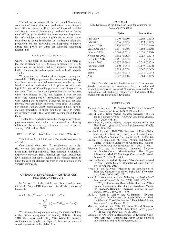
We estimate this equation allowing for serial correlationin the residual, using data from January 2004 to February2010, where t0 is equal to July 2009. While the estimatedcoefficients are graphed in Figure 5, here we provide theactual regression results (Table A1).

TABLE A1DID Estimates of the Impact of Cash-for-Clunkers for

Sales and Production

Sales Production

June 2009 0.040 (0.060) 0.205 (0.108)July 2009 0.296 (0.072) 0.153 (0.117)August 2009 0.479 (0.077) 0.077 (0.119)September 2009 −0.201 (0.080) −0.108 (0.120)October 2009 −0.094 (0.081) −0.036 (0.120)November 2009 −0.112 (0.082) −0.053 (0.121)December 2009 −0.161 (0.083) −0.235 (0.121)January 2010 −0.137 (0.084) −0.048 (0.122)February 2010 −0.190 (0.084) −0.149 (0.122)Constant 0.593 (0.039) 0.647 (0.042)Trend 0.018 (0.001) 0.018 (0.001)AR(1) 0.607 (0.100) 0.364 (0.117)

Note: See the text for details on the DID estimation.Standard errors are in parentheses. Both the sales andproduction regressions included 74 observations and the R-squared are 0.98 and 0.94, respectively. The units of thecoefficients are logarithmic deviations.

REFERENCES

Abrams, B. A., and G. R. Parsons. “Is CARS a Clunker?”The Economists’ Voice, 6(8), 2009, article 4.

Bils, M., and J. Kahn. “What Inventory Behavior Tells Usabout Business Cycles.” American Economic Review,90(3), 2000, 458–81.

Bresnahan, T., and V. Ramey. “Output Fluctuations at thePlant Level.” Quarterly Journal of Economics, 109(3),1994, 593–624.

Copeland, A., and G. Hall. “The Response of Prices, Sales,and Output to Temporary Changes in Demand.” Jour-nal of Applied Econometrics, 26(no. 2), 2011, 232–69.

Erdem, T., S. Imai, and M. Keane. “Brand and QuantityChoice Dynamics under Price Uncertainty.” Quanti-tative Marketing and Economics, 1(1), 2003, 5–64.

Feldstein, M., and A. Auerbach. “Inventory Behaviorin Durable-Goods Manufacturing: The Target-Adjustment Model.” Brookings Papers on EconomicActivity, 2, 1976, 351–408.

Gowrisankaran, G., and M. Rysman. “Dynamics of Demandfor New Durable Goods.” Unpublished Paper, Univer-sity of Arizona, 2010.

Hendel, I., and A. Nevo. “Measuring the Implications ofSales and Consumer Inventory Behavior.” Economet-rica, 74(6), 2006, 1637–73.

Kahn, J. “Inventories and the Volatility of Production.”American Economic Review, 77(4), 1987, 667–79.

. “Why Is Production More Volatile than Sales? The-ory and Evidence on the Stockout-Avoidance Motivefor Inventory-Holding.” Quarterly Journal of Eco-nomics, 107(2), 1992, 481–510.

Li, S., J. Linn, E. Spiller, and C. Timmins. “Evaluat-ing ‘Cash for Clunkers’: Program Effect on Vehi-cle Sales and Cost-Effectiveness.” Unpublished Paper,Resources for the Future, 2010.

Mian, A., and A. Sufi. “The Effects of Fiscal Stimulus:Evidence from the 2009 ‘Cash for Clunkers’ Program.”NBER Working Paper no. 16351, 2010.

Schiraldi, P. “Automobile Replacement: A Dynamic Struc-tural Approach.” Unpublished Paper, London Schoolof Economics and Political Science, 2010.

Documents

THE PRODUCTION IMPACT OF “CASH-FOR-CLUNKERS”: IMPLICATIONS FOR STABILIZATION POLICY