Embed Size (px)
Citation preview
COMPUTED TOMOGRAPHY (I)
RAD 365
CT - Scan
Prepared By:Ala’a Ali Tayem Abed
The production of X-RaysX-Rays are produced whenever charged particles are slowed down or stopped.
X-rays are generated via interactions of the accelerated electrons with electrons of tungsten nuclei within the tube anode. There are two types of X-ray generated: Characteristic radiation and Bremsstrahlung radiation.
1. Characteristic X-ray generation: When a high energy electron, collides with an inner shell electron, both are ejected from the tungsten atom leaving a 'hole' in the inner layer. This is filled by an outer shell electron with a loss of energy emitted as an X-ray photon.
2. Bremsstrahlung/Braking X-ray generation: When an electron passes near the nucleus it is slowed and its path is deflected. Energy lost is emitted as a bremsstrahlung X-ray photon. Bremsstrahlung = Braking. Approximately 80% of the population of X-rays within the X-ray beam consists of X-rays generated in this way.
X-Ray Interactions
Interaction of X-Rays with matterWhen a beam of X-Rays passes through matter, its intensity is reduced as the energy is absorbed or scattered.The degree of attenuation depends on the atomic number and physical density of the tissue, and the energy of the X-Rays.The differential absorption of X-Rays by the various tissues of the patient allows a radiographic image to be made.
Recall that photons are individual units of energy. As an x-ray beam passes through an object, three possible fates await each photon, as shown in the figure below:1. It can penetrate the section of matter without interacting.2. It can interact with the matter and be completely absorbed by depositing its energy.3. It can interact and be scattered or deflected from its original direction and deposit part of its energy.
There are two kinds of interactions through which photons deposit their energy; both are with electrons. In one type of interaction the photon loses all its energy; in the other, it loses a portion of its energy, and the remaining energy is scattered
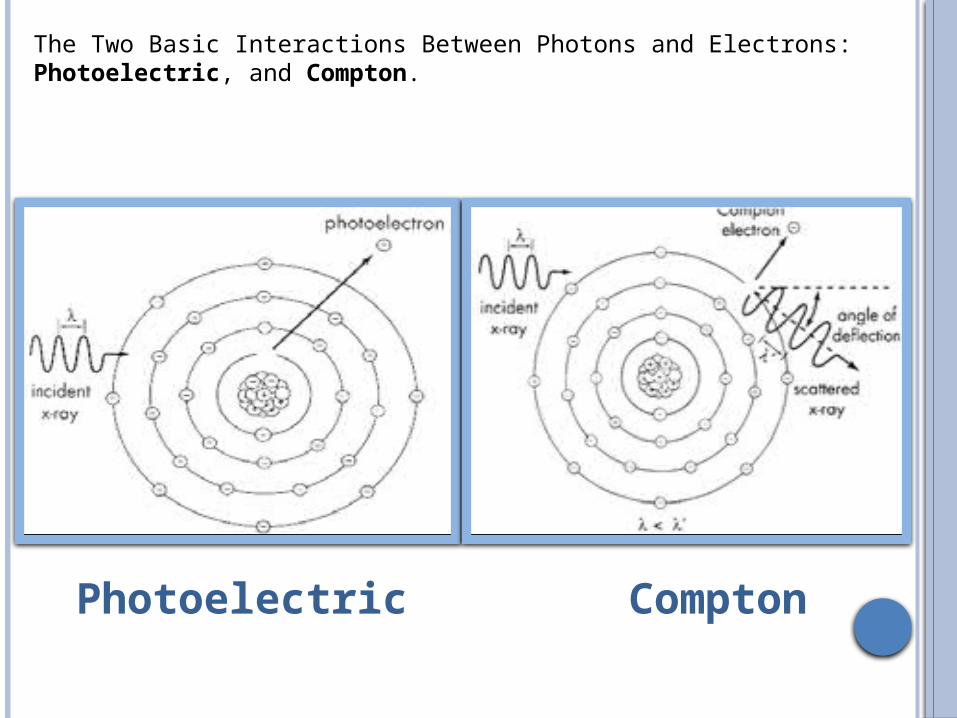
The Two Basic Interactions Between Photons and Electrons: Photoelectric, and Compton.
Photoelectric Compton
Interaction Between Penetrating Radiation and Matter
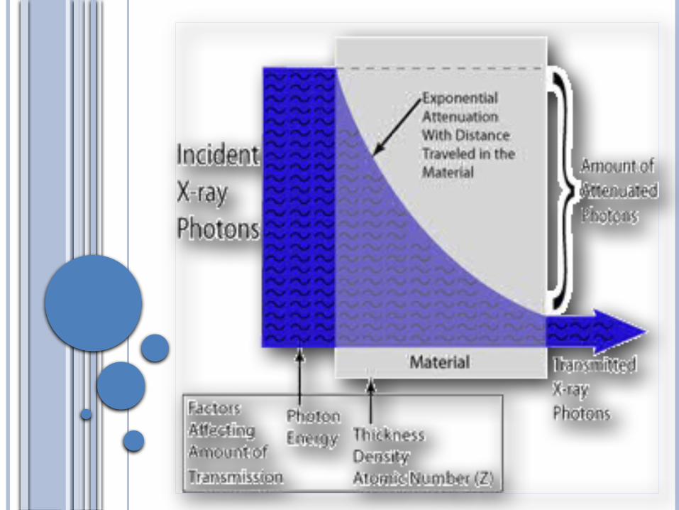
When x-rays are directed into an object, some of the photons interact with the particles of the matter and their energy can be absorbed or scattered.
This absorption and scattering is called attenuation.
Other photons travel completely through the object without interacting with any of the material's particles.
The number of photons transmitted through a material depends on the:1. Thickness.2. Density.3. Atomic Number of the Material.4. Energy of the Individual Photons. 5. The number of photons reaching a specific point within the matter decreases exponentially with distance traveled.
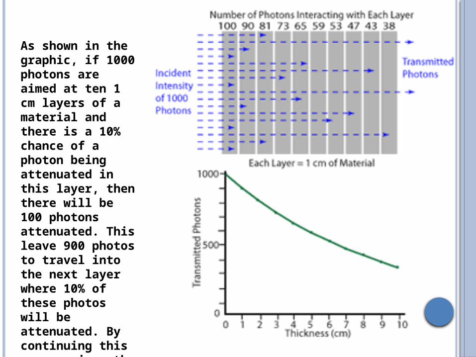
As shown in the graphic, if 1000 photons are aimed at ten 1 cm layers of a material and there is a 10% chance of a photon being attenuated in this layer, then there will be 100 photons attenuated. This leave 900 photos to travel into the next layer where 10% of these photos will be attenuated. By continuing this progression, the exponential shape of the curve becomes apparent.
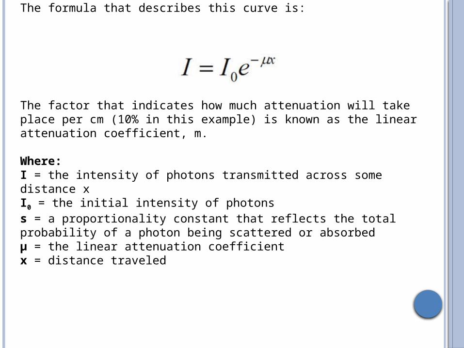
The formula that describes this curve is:
The factor that indicates how much attenuation will take place per cm (10% in this example) is known as the linear attenuation coefficient, m. Where:I = the intensity of photons transmitted across some distance x I0 = the initial intensity of photons s = a proportionality constant that reflects the total probability of a photon being scattered or absorbedµ = the linear attenuation coefficient x = distance traveled
The Linear Attenuation Coefficient (µ)
The linear attenuation coefficient (µ) describes the fraction of a beam of x-rays that is absorbed or scattered per unit thickness of the absorber.
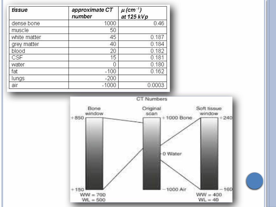
CT images are a display of the amount of attenuation that has occurred when the X-ray beam penetrates the body - this is known as the linear attenuation coefficient. The density measurement of this attenuated beam is assigned a CT number (Hounsfield Units) which are related to this linear attenuation coefficient. The selection of kVp has a direct effect on these linear coefficients values.
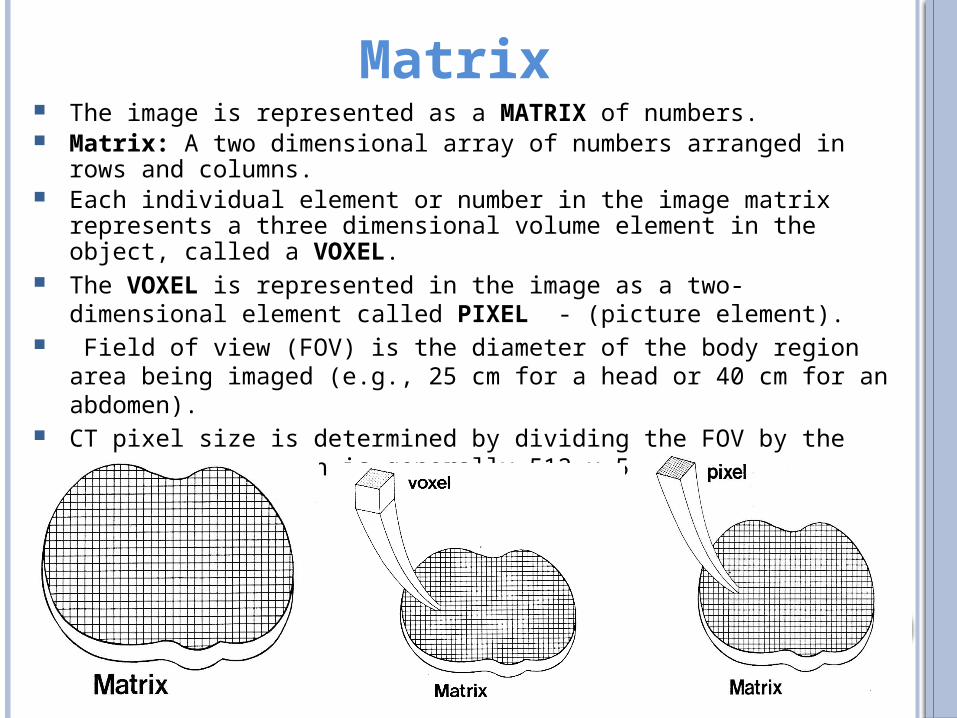
Matrix The image is represented as a MATRIX of numbers. Matrix: A two dimensional array of numbers arranged in rows and columns. Each individual element or number in the image matrix represents a three dimensional
volume element in the object, called a VOXEL. The VOXEL is represented in the image as a two-dimensional element called PIXEL
- (picture element). Field of view (FOV) is the diameter of the body region area being imaged (e.g., 25
cm for a head or 40 cm for an abdomen). CT pixel size is determined by dividing the FOV by the matrix size, which is
generally 512 x 512 in CT.
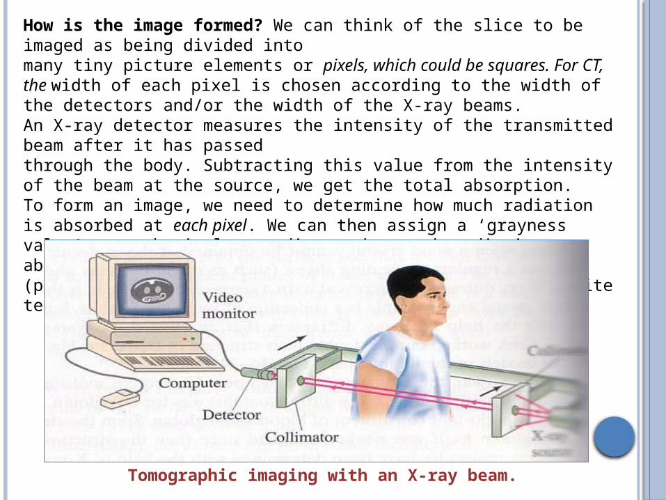
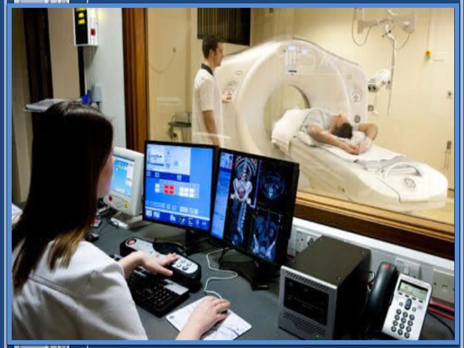
How is the image formed? We can think of the slice to be imaged as being divided intomany tiny picture elements or pixels, which could be squares. For CT, the width of each pixel is chosen according to the width of the detectors and/or the width of the X-ray beams. An X-ray detector measures the intensity of the transmitted beam after it has passedthrough the body. Subtracting this value from the intensity of the beam at the source, we get the total absorption.To form an image, we need to determine how much radiation is absorbed at each pixel. We can then assign a ‘grayness value’ to each pixel according to how much radiation was absorbed. The image, then, is made up of tiny spots (pixels) of varying shades of grey, as is a black-and-white television picture.
Tomographic imaging with an X-ray beam.
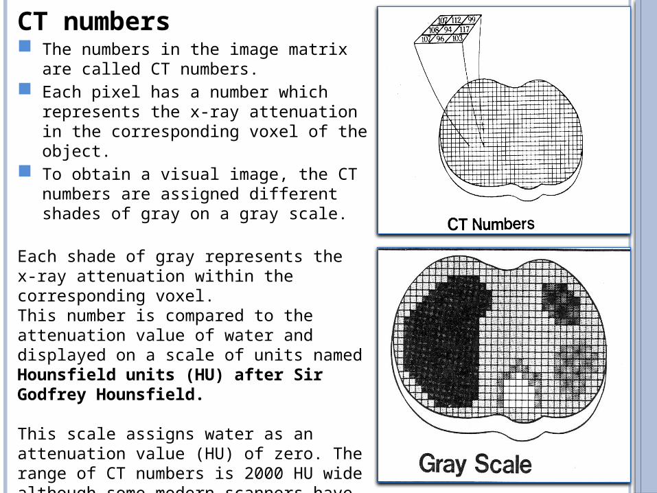
CT numbers The numbers in the image matrix are called CT
numbers. Each pixel has a number which represents the x-
ray attenuation in the corresponding voxel of the object.
To obtain a visual image, the CT numbers are assigned different shades of gray on a gray scale.
Each shade of gray represents the x-ray attenuation within the corresponding voxel. This number is compared to the attenuation value of water and displayed on a scale of units named Hounsfield units (HU) after Sir Godfrey Hounsfield.
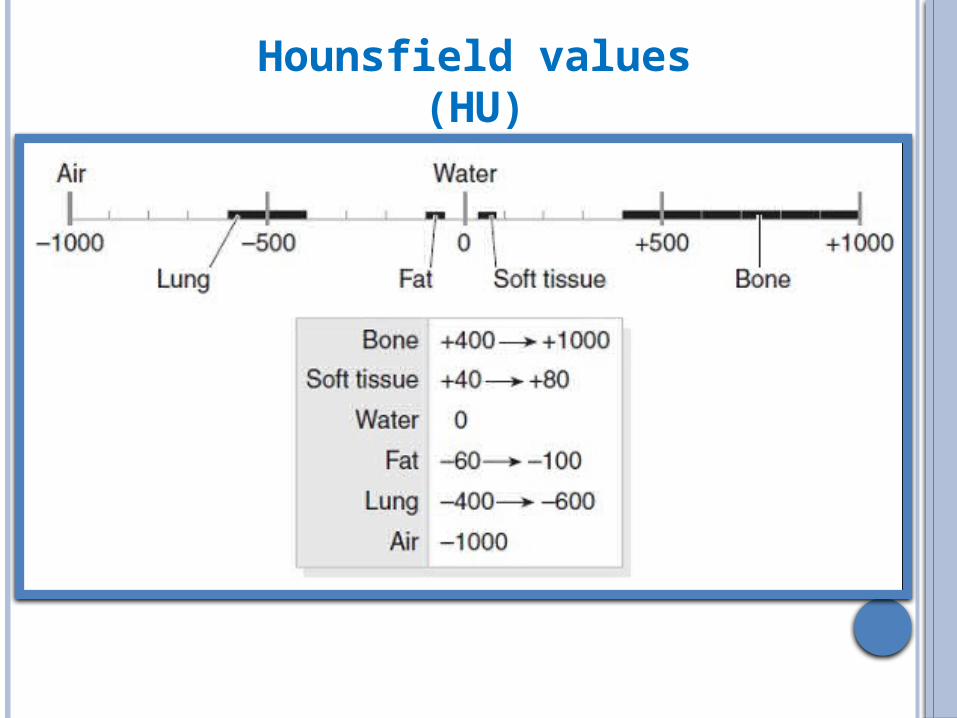
This scale assigns water as an attenuation value (HU) of zero. The range of CT numbers is 2000 HU wide although some modern scanners have a greater range of HU up to 4000. Each number represents a shade of grey with +1000 (white) and –1000 (black) at either end of the spectrum.
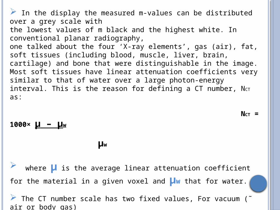
In the display the measured m-values can be distributed over a grey scale withthe lowest values of m black and the highest white. In conventional planar radiography,one talked about the four ‘X-ray elements’, gas (air), fat, soft tissues (including blood, muscle, liver, brain, cartilage) and bone that were distinguishable in the image. Most soft tissues have linear attenuation coefficients very similar to that of water over a large photon-energy interval. This is the reason for defining a CT number, NCT as:
NCT = 1000× μ – μw
μw
where μ is the average linear attenuation coefficient for the material in a given voxel
and μw that for water.
The CT number scale has two fixed values, For vacuum (˜ air or body gas) NCT, vac = -1000 and for water NCT water = 0.
CT number affected by kVp – Reduce kVp, increase contrast.
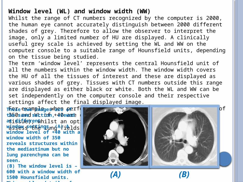
Window level (WL) and window width (WW)Whilst the range of CT numbers recognized by the computer is 2000, the human eye cannot accurately distinguish between 2000 different shades of grey. Therefore to allow the observer to interpret the image, only a limited number of HU are displayed. A clinically useful grey scale is achieved by setting the WL and WW on the computer console to a suitable range of Hounsfield units, depending on the tissue being studied.The term ‘window level’ represents the central Hounsfield unit of all the numbers within the window width. The window width covers the HU of all the tissues of interest and these are displayed as various shades of grey. Tissues with CT numbers outside this range are displayed as either black or white. Both the WL and WW can be set independently on the computer console and their respective settings affect the final displayed image.For example, when performing a CT examination of the chest, a WW of 350 and WL of +40 are chosen to image the mediastinum (soft tissue), whilst an optimal WW of 1500 and WL of –600 are used to assess the lung fields (mostly air).
These two images are of the same section, viewed at differentwindow settings. (A) A window level of +40 with a window width of 350reveals structures within the mediastinum but no lung parenchyma can be seen.(B) The window level is –600 with a window width of 1500 Hounsfield units. This enables details of the lung parenchyma to be seen, at the expense of the mediastinum. (A) (B)
Hounsfield values (HU)
CT IMAGE RECONSTRUCTION
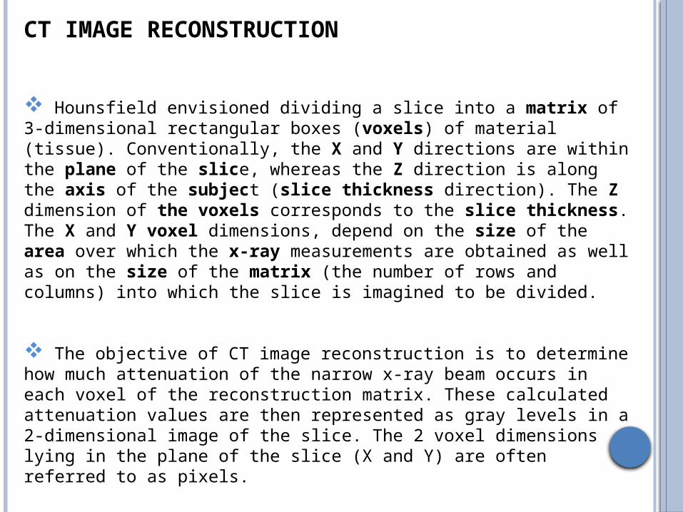
Hounsfield envisioned dividing a slice into a matrix of 3-dimensional rectangular boxes (voxels) of material (tissue). Conventionally, the X and Y directions are within the plane of the slice, whereas the Z direction is along the axis of the subject (slice thickness direction). The Z dimension of the voxels corresponds to the slice thickness. The X and Y voxel dimensions, depend on the size of the area over which the x-ray measurements are obtained as well as on the size of the matrix (the number of rows and columns) into which the slice is imagined to be divided.
The objective of CT image reconstruction is to determine how much attenuation of the narrow x-ray beam occurs in each voxel of the reconstruction matrix. These calculated attenuation values are then represented as gray levels in a 2-dimensional image of the slice. The 2 voxel dimensions lying in the plane of the slice (X and Y) are often referred to as pixels.
CT IMAGE RECONSTRUCTION
The Radon transform is widely applicable to tomography, the creation of an image from
the projection data associated with cross-sectional scans of an object. If a function ƒ
represents an unknown density, then the Radon transform represents the projection data
obtained as the output of a tomographic scan. Hence the inverse of the Radon transform
can be used to reconstruct the original density from the projection data, and thus it forms
the mathematical underpinning for tomographic reconstruction, also known as image
reconstruction.
Ray, Ray sum, View & Attenuation Profile Ray – Imaginary line between Tube & Detector. Ray Sum – Attenuation along a Ray. View – The set of ray sums in one direction. The attenuation for each ray sum when plotted as function of its position is called an
attenuation profile. Attenuation of objects with different densities will change the attenuation profile.
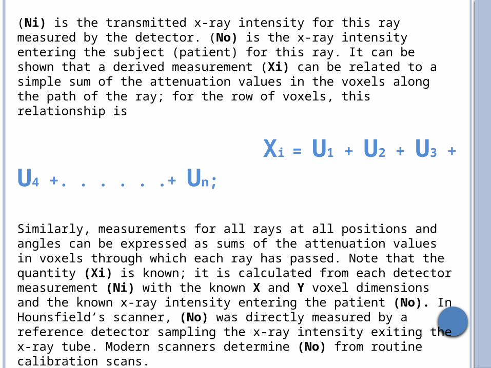
(Ni) is the transmitted x-ray intensity for this ray measured by the detector. (No) is the x-ray intensity entering the subject (patient) for this ray. It can be shown that a derived measurement (Xi) can be related to a simple sum of the attenuation values in the voxels along the path of the ray; for the row of voxels, thisrelationship is
Xi = U1 + U2 + U3 + U4 +. . . . . .+ Un;
Similarly, measurements for all rays at all positions and angles can be expressed as sums of the attenuation values in voxels through which each ray has passed. Note that the quantity (Xi) is known; it is calculated from each detector measurement (Ni) with the known X and Y voxel dimensions and the known x-ray intensity entering the patient (No). In Hounsfield’s scanner, (No) was directly measured by a reference detector sampling the x-ray intensity exiting the x-ray tube. Modern scanners determine (No) from routine calibration scans.