The Projection Dynamicand the Replicator Dynamic∗

William H. Sandholm†, Emin Dokumacı‡, and Ratul Lahkar§

February 1, 2008

Abstract

We investigate a variety of connections between the projection dynamic and thereplicator dynamic. At interior population states, the standard microfoundations forthe replicator dynamic can be converted into foundations for the projection dynamicby replacing imitation of opponents with “revision driven by insecurity” and directchoice of alternative strategies. Both dynamics satisfy a condition called inflow-outflow symmetry, which causes them to select against strictly dominated strategiesat interior states; still, because it is discontinuous at the boundary of the state space, theprojection dynamic allows strictly dominated strategies to survive in perpetuity. Thetwo dynamics exhibit qualitatively similar behavior in strictly stable and null stablegames. Finally, the projection and replicator dynamics both can be viewed as gradientsystems in potential games, the latter after an appropriate transformation of the statespace. JEL classification: C72, C73.

1. Introduction

The projection dynamic is an evolutionary game dynamic introduced in the transporta-tion science literature by Nagurney and Zhang (1996). Microfoundations for this dynamic

∗We thank two anonymous referees, an anonymous Associate Editor, and many seminar audiencesfor helpful comments. Financial support from NSF Grants SES-0092145 and SES-0617753 is gratefullyacknowledged.†Department of Economics, University of Wisconsin, 1180 Observatory Drive, Madison, WI 53706, USA.

e-mail: whs@ssc.wisc.edu, website: http://www.ssc.wisc.edu/∼whs.‡Department of Economics, University of Wisconsin, 1180 Observatory Drive, Madison, WI 53706, USA.

e-mail: edokumaci@wisc.edu, website: http://www.ssc.wisc.edu/∼edokumac.§Department of Mathematics and ELSE, University College London, Gower Street, London WC1E6BT,

UK. e-mail: r.lahkar@ucl.ac.uk, website: http://rlahkar.googlepages.com.

are provided in Lahkar and Sandholm (2008): there the dynamic is derived from a modelof “revision driven by insecurity”, in which each agent considers switching strategies at arate inversely proportional to his current strategy’s popularity. Although it is discontin-uous at the boundary of the state space, the projection dynamic admits unique forwardsolution trajectories; its rest points are the Nash equilibria of the underlying game, andit converges to equilibrium from all initial conditions in potential games and in stablegames.

In this paper, we investigate the many connections between the projection dynamicand the replicator dynamic of Taylor and Jonker (1978). Our companion paper, Lahkar andSandholm (2008), established one link between the dynamics’ foundations. In general,one provides foundations for an evolutionary dynamic by showing that it is the meandynamic corresponding to a particular revision protocol—that is, a particular rule usedby agents to decide when and how to choose new strategies.1 The companion paper findsa new revision protocol that generates the replicator dynamic, and shows that a suitablemodification of this protocol generates the projection dynamic.

In economic contexts, the replicator dynamic is best understood as a model of imita-tion. In Lahkar and Sandholm (2008), a principal step in changing the replicator protocolinto a projection protocol is to eliminate the former’s use of imitation, replacing this with“revision driven by insecurity” and direct (nonimitative) selection of alternative strate-gies. But if we look only at behavior at interior population states—that is, at states whereall strategies are in use—then this one step becomes sufficient for converting replicatorprotocols into projection protocols. To be more precise, we show in Section 3 that foreach of the three standard foundations for the replicator dynamic (due to Schlag (1998),Bjornerstedt and Weibull (1996), and Hofbauer (1995)), replacing “imitation” with “revi-sion driven by insecurity” yields a foundation for the projection dynamic valid at interiorpopulation states.

Both “imitation” and “revision driven by insecurity” are captured formally by directlyincluding components of the population state in the outputs of revision protocols. Weshow that the precise ways in which these arguments appear lead the replicator andprojection dynamics to satisfy a property called inflow-outflow symmetry at interior popu-lation states. Inflow-outflow symmetry implies that any strictly dominated strategy mustalways be “losing ground” to its dominating strategy, pushing the weight on the domi-nated strategy toward zero. Akin (1980) uses this observation to show that the replicatordynamic eliminates strictly dominated strategies along all interior solution trajectories.

This elimination result does not extend to the projection dynamic. Using the fact that

1For formal statements of this idea, see Benaım and Weibull (2003) and Sandholm (2003).

–2–

solutions of the projection dynamic can enter and leave the boundary of the state space, weconstruct an example in which a strictly dominated strategy appears and then disappearsfrom the population in perpetuity. Because the projection dynamic is discontinuous, thefact that the dominated strategy is losing ground to the dominating strategy at all interiorpopulation states is not enough to ensure its eventual elimination.2

The final section of the paper compares the global behavior of the two dynamicsin two important classes of games: stable games and potential games. In the formercase, the properties of the two dynamics mirror one another: one can establish (interior)global asymptotic stability for both dynamics in strictly stable games, and the existenceof constants of motion in null stable games, including zero-sum games.3

The connection between the projection and replicator dynamics in potential gamesis particularly striking. On the interior of the state space, the projection dynamic for apotential game is the gradient system generated by the game’s potential function: interiorsolutions of the dynamic always ascend potential in the most direct fashion. The linkwith the replicator dynamic arises by way of a result of Akin (1979). Building on workof Kimura (1958) and Shahshahani (1979), Akin (1979) shows that the replicator dynamicfor a potential game is also a gradient system defined by the game’s potential function;however, this is true only after the state space has been transformed by a nonlinearchange of variable, one that causes greater importance to be attached to changes in theuse of rare strategies. We conclude the paper with a direct proof of Akin’s (1979) result:unlike Akin’s (1979) original proof, ours does not require the introduction of tools fromdifferential geometry.

In summary, this paper argues that despite a basic difference between the two dynamics—that one is based on imitation of opponents, and the other on “revision driven by inse-curity” and direct selection of new strategies—the replicator dynamic and the projectiondynamic exhibit surprisingly similar behavior.

2. Definitions

To keep the presentation self-contained, we briefly review some definitions and resultsfrom Lahkar and Sandholm (2008).

2Hofbauer and Sandholm (2006), building on the work of Berger and Hofbauer (2006), construct a gamethat possesses a strictly dominated strategy, but that causes a large class of evolutionary dynamics to admitan interior attractor. The analysis in that paper concerns dynamics that are continuous in the populationstate, and therefore does not apply to the projection dynamic.

3In contrast, other standard dynamics, including the best response, logit, BNN, and Smith dynamics,converge to equilibrium in null stable games: see Hofbauer and Sandholm (2008, 2007).

–3–

2.1 Preliminaries

To simplify our notation, we focus on games played by a single unit-mass populationof agents who choose pure strategies from the set S = {1, . . . ,n}. The set of population states(or strategy distributions) is thus the simplex X = {x ∈ Rn

+ :∑

i∈S xi = 1}, where the scalarxi ∈ R+ represents the mass of players choosing strategy i ∈ S.

We take the strategy set S as given and identify a population game with its payofffunction F : X → Rn, a Lipschitz continuous map that assigns each population state x avector of payoffs F(x). The component function Fi : X→ R denotes the payoffs to strategyi ∈ S. State x ∈ X is a Nash equilibrium of F, denoted x ∈ NE(F), if xi > 0 implies thati ∈ argmax j∈S F j(x).

The tangent space of X, denoted TX = {z ∈ Rn :∑

i∈S zi = 0}, contains those vectorsdescribing motions between points in X. The orthogonal projection onto the subspaceTX ⊂ Rn is represented by the matrix Φ = I − 1

n11′ ∈ Rn×n, where 1 = (1, ..., 1)′ is the vectorof ones. Since Φv = v − 1 · 1

n

∑k∈S vk, component (Φv)i is the difference between the vi

and the unweighted average payoff of the components of v. Thus, if v is a payoff vector,Φv discards information about the absolute level of payoffs while preserving informationabout relative payoffs.

The tangent cone of X at state x ∈ X is the set of directions of motion from x that initiallyremain in X:

TX(x) = {z ∈ Rn : z = α(y − x) for some y ∈ X and some α ≥ 0}

= {z ∈ TX : zi ≥ 0 whenever xi = 0}.

The closest point projection onto TX(x) is given by

ΠTX(x)(v) = argminz∈TX(x)

∣∣∣z − v∣∣∣ .

It is easy to verify that if x ∈ int(X), then TX(x) = TX, so that ΠTX(x)(v) = Φv. Moregenerally, Lahkar and Sandholm (2008) show that

(1) (ΠTX(x)(v))i =

vi −1

#S (v,x)

∑j∈S (v,x) v j if i ∈ S (v, x),

0 otherwise,

where the set S (v, x) ⊆ S contains all strategies in support(x), along with any subset ofS − support(x) that maximizes the average 1

#S (v,x)

∑j∈S (v,x) v j.

–4–

2.2 The Replicator Dynamic and the Projection Dynamic

An evolutionary dynamic is a map that assigns each population game F a differentialequation x = VF(x) on the state space X. The best-known evolutionary dynamic is thereplicator dynamic (Taylor and Jonker (1978)), defined by

(R) xi = xi

Fi(x) −∑k∈S

xkFk(x)

.In words, equation (R) says that the percentage growth rate of strategy i equals the differencebetween the payoff to strategy i and the weighted average payoff under F at x (that is, theaverage payoff obtained by members of the population).

The projection dynamic (Nagurney and Zhang (1997)) assigns each population game Fthe differential equation

(P) x = ΠTX(x)(F(x)).

Under the projection dynamic, the direction of motion is always given by the closestapproximation of the payoff vector F(x) by a feasible direction of motion. When x ∈ int(X),the tangent cone TX(x) is just the subspace TX, so the explicit formula for (P) is simplyx = ΦF(x); otherwise, the formula is obtained from equation (1).

To begin to draw connections between the two dynamics, note that at interior popula-tion states, the projection dynamic can be written as4

(2) xi = (ΦF(x))i = Fi(x) −1n

∑i∈S

Fk(S).

In words, the projection dynamic requires the absolute growth rate of strategy i to be thedifference between strategy i’s payoff and the unweighted average payoff of all strategies.5

Comparing equations (R) and (2), we see that at interior population states, the replicatorand projection dynamics convert payoff vector fields in differential equations in similarfashions, the key difference being that the replicator dynamic uses relative definitions,while the projection dynamic employs the corresponding absolute definitions. The re-mainder of this paper explores game-theoretic ramifications of this link.

When F is generated by random matching to play the normal form game A (i.e., when

4At interior population states (but not boundary states), the projection dynamic is identical to the lineardynamic of Friedman (1991); see Lahkar and Sandholm (2008) for further discussion.

5At boundary states, some poorly performing unused strategies (namely, those not in S (F(x), x)) areignored, while the absolute growth rates of the remaining strategies are defined as before.

–5–

F takes the linear form F(x) = Ax), the dynamic (P) is especially simple. On int(X), thedynamic is described by the linear equation x = ΦAx; more generally, it is given by

(3) xi = (ΠTX(x)(Ax))i =

(Ax)i −1

#S (Ax,x)

∑j∈S (Ax,x)(Ax) j if i ∈ S (Ax, x),

0 otherwise.

Notice that once the set of strategies S (Ax, x) is fixed, the right hand side of (3) is a linearfunction of x. Thus, under single population random matching, the projection dynamic ispiecewise linear. In Section 4, this observation plays a key role in our proof that strictlydominated strategies can survive under (P).

3. Microfoundations

We derive evolutionary dynamics from a description of individual behavior by intro-ducing the notion of a revision protocol ρ : Rn

× X → Rn×n+ . Suppose that as time passes,

agents are randomly offered opportunities to switch strategies. The conditional switch rateρi j(F(x), x) ∈ R+ is proportional to the probability with which an i player who receives anopportunity switches to strategy j.

Given this specification of individual decision making, aggregate behavior in the gameF is described by the mean dynamic

(M) xi =∑j∈S

x jρ ji(F(x), x) − xi

∑j∈S

ρi j(F(x), x).

Here the first term describes the inflow into strategy i from other strategies, while thesecond term describes the outflow from i to other strategies.

Consider these three examples of revision protocols:

ρi j = x j[F j(x) − Fi(x)]+,(4a)

ρi j = x j(K − Fi(x)),(4b)

ρi j = x j(F j(x) + K).(4c)

The x j term in these three protocols reveals that they are models of imitation. For instance,to implement protocol (4a), an agent who receives a revision opportunity picks an op-ponent from at random; he then imitates this opponent only if the opponents’ payoff ishigher than his own, doing so with probability proportional to the payoff difference.6

6Protocol (4a) is the pairwise proportional imitation protocol of Schlag (1998); protocol (4b), called pure

–6–

It is well known that the replicator dynamic can be viewed as the aggregate result ofevolution by imitation. In fact, all three protocols above generate the replicator dynamicas their mean dynamics. For protocol (4a), one computes that

xi =∑j∈S

x jρ ji − xi

∑j∈Sρi j

=∑j∈S

x jxi[Fi(x) − F j(x)]+− xi

∑j∈S

x j[F j(x) − Fi(x)]+

= xi

∑j∈S

x j(Fi(x) − F j(x))

= xi

Fi(x) −∑j∈S

x jF j(x)

.The derivations for the other two protocols are similar.

To draw connections with the projection dynamic, we replace the x j term with 1nxi

ineach of the protocols above:

ρi j =1

nxi[F j(x) − Fi(x)]+,(5a)

ρi j =1

nxi(K − Fi(x)),(5b)

ρi j =1

nxi(F j(x) + K).(5c)

While protocols (4a)–(4c) captured imitation, protocols (5a)–(5c) instead capture revisiondriven by insecurity: agents are quick to abandon strategies that are used by few of theirfellows. For instance, under protocol (5a), an agent who receives a revision opportunityfirst considers whether to actively reconsider his choice of strategy, opting to do so withprobability inversely proportional to the mass of agents currently choosing his strategy.If he does consider revising, he chooses a strategy at random, and then switches to thisstrategy with probability proportional to the the difference between its payoff and hiscurrent payoff.

Protocols (5a)–(5c) are only well-defined on int(X). But on that set, each of the protocolsgenerates the projection dynamic. For protocol (5a), this is verified as follows:

xi =∑j∈S

x jρ ji − xi

∑j∈S

ρi j

imitation driven by dissatisfaction, is due to Bjornerstedt and Weibull (1996), protocol (4c), which we callimitation of success, can be found in Hofbauer (1995).

–7–

=∑j∈S

x j[Fi(x) − F j(x)]

+

nx j− xi

∑j∈S

[F j(x) − Fi(x)]+

nxi

=1n

∑j∈S

(Fi(x) − F j(x))

= Fi(x) −1n

∑j∈S

F j(x).

Again, the derivations for the other protocols are similar.On the boundary of the simplex X, protocols (5a)–(5c) no longer make sense. Still, it is

possible to construct a matched pair of revision protocols that generate dynamics (R) and(P) throughout the simplex—see Lahkar and Sandholm (2008) for details.

4. Inflow-Outflow Symmetry and Dominated Strategies

It is natural to expect evolutionary dynamics to eliminate dominated strategies. Thefirst positive result on this question was proved by Akin (1980), who showed that thereplicator dynamic eliminates strictly dominated strategies so long as the initial state isinterior. Akin’s (1980) result was subsequently extended to broader classes of imitativedynamics by Samuelson and Zhang (1992) and Hofbauer and Weibull (1996). But whilethese results seem encouraging, they are actually quite special: Hofbauer and Sandholm(2006) show that continuous evolutionary dynamics that are not based exclusively onimitation do not eliminate strictly dominated strategies in all games.

In this section, we show that the projection dynamic shares with the replicator dynamica property called inflow-outflow symmetry, and we explain why this property leads toselection against dominated strategies on the interior of X under both of these dynamics.Despite this shared property of the two dynamics, the long run prospects for dominatedstrategies under these dynamics are quite different. Using the fact that solutions to theprojection dynamic can enter and exit the boundary of X, we prove that inflow-ouflowsymmetry is not enough to ensure that dominated strategies are eliminated.

In the general expression for the mean dynamic (M),

(M) xi =∑j∈S

x jρ ji(F(x), x) − xi

∑j∈S

ρi j(F(x), x),

the term xi, representing the mass of players choosing strategy i, appears in an asymmetricfashion. Since in order for an agent to switch away from strategy i, he must first be selectedat random for a revision opportunity, xi appears in the (negative) outflow term. But since

–8–

agents switching to strategy i were previously playing other strategies, xi does not appearin the inflow term.

We say that an evolutionary dynamic satisfies inflow-outflow symmetry if this asym-metry in equation (M) is eliminated by the dependence of the revision protocol ρ on thepopulation state x. Under the replicator dynamic and other imitative dynamics, ρ ji isproportional to xi, making both the inflow and outflow terms in (M) proportional to xi;thus, these dynamics exhibit inflow-outflow symmetry. Similarly, under the projectiondynamic, which is based on abandonment, ρi j is inversely proportional to xi whenever xi

is positive. As a result, neither the inflow nor the outflow term in equation (M) dependsdirectly on xi, yielding inflow-ouflow symmetry on int(X).

Importantly, inflow-outflow symmetry implies that a strictly dominated strategy iwill always lose ground to the strategy j that dominates it. In the case of the replicatordynamic, the ratio xi/x j falls over time throughout int(X):

ddt

(xi

x j

)=

xix j − x jxi

x2j

(6)

=xi

(Fi(x) −

∑k∈S xkFk(x)

)· x j − x j

(F j(x) −

∑k∈S xkFk(x)

)· xi

x2j

=xi

x j(Fi(x) − F j(x))

< 0.

Under the the projection dynamic, it is the difference xi − x j that falls on int(X):

ddt

(xi − x j

)=

Fi(x) − 1n

∑k∈S

Fk(x)

−F j(x) − 1

n

∑k∈S

Fk(x)

(7)

= Fi(x) − F j(x)

< 0.

By combining equation (6) with the fact that int(X) is invariant under (R), it is easy toprove that the replicator dynamic eliminates strictly dominated strategies along solutionsin int(X); this is Akin’s (1980) result. But because solutions of the projection dynamiccan enter and leave int(X), the analogous argument based on equation (7) does not gothrough: while i will lose ground to j in the interior of X, it might gain ground back onthe boundary of X, leaving open the possibility of survival.

To pursue this idea, we consider the following game, introduced by Berger and Hof-

–9–

bauer (2006) in their analysis of survival of dominated strategies under the BNN dynamic:

(8) F(x) = Ax =

0 −3 2 22 0 −3 −3−3 2 0 0−3 − c 2 − c −c −c

xR

xP

xS

xT

.The game defined by the first three strategies is bad Rock-Paper-Scissors with winningbenefit w = 2 and losing cost l = 3. In this three-strategy game, solutions of (P) other thanthe one at the Nash equilibrium (1

3 ,13 ,

13 ) enter a closed orbit that enters and exits the three

edges of the simplex (see Figure 7(iii) of Lahkar and Sandholm (2008)).The fourth strategy of game (8), Twin, is a duplicate of Scissors, except that its payoff is

always c ≥ 0 lower than that of Scissors. When c = 0, the set of Nash equilibria of game (8)is the line segment L between x∗ = ( 1

3 ,13 ,

13 , 0) and ( 1

3 ,13 , 0,

13 ). If c > 0, then Twin is strictly

dominated, and the game’s unique Nash equilibrium is x∗.Figure 1 presents the solution to (P) from initial condition ( 97

300 ,103300 ,

1100 ,

97300 ) for payoff

parameter c = 110 . At first, the trajectory spirals down line segment L, as agents switch

from Rock to Paper to Scissors/Twin to Rock, with Scissors replacing Twin as time passes(since xT− xS = −

110 on int(X)). When Twin is eliminated, both it and Scissors earn less than

the average of the payoffs to Rock, Paper, and Scissors; therefore, xS falls while xT staysfixed at 0, and so xT − xS rises. Soon the solution enters int(X), and so xT − xS = −

110 once

again. When the solution reenters face RPS, it does so at a state further away from theNash equilibrium x∗ than the initial point of contact. Eventually, the trajectory appears toenter a closed orbit on which the mass on Twin varies between 0 and roughly .36.

The existence and stability of this closed orbit is established rigorously in Theorem 4.1,whose proof can be found in the appendix.

Theorem 4.1. In game (8) with c = 110 , the projection dynamic (P) has an asymptotically stable

closed orbit γ that absorbs all solutions from nearby states in finite time. This orbit, picturedin Figure 2, combines eight segments of solutions to linear differential equations as described inequation (3); the approximate endpoints and exit times of these segments are presented in Table 1.Along the orbit, the value of xT varies between 0 and approximately .359116.

Recall that in random matching games, the projection dynamic is piecewise linear:on the interior of X, the dynamic is described by x = ΦAx; on the boundary of X, itis described by equation (3). When the only unused strategy is strategy i, equation (3)provides only two possibilities for x: if Fi(x) does not exceed the average payoff of theother three strategies, then xi = 0, so the solution travels along the face of X where strategy

–10–

R

P

S T

Figure 1: A solution to (P) in Bad Rock-Paper-Scissors-Twin.

i is absent; if instead Fi(x) is greater than this average payoff, then the solution from ximmediately enters int(X). We illustrate these regions in Figure 2, where we shade theportions of the faces of X to which solutions “stick”.

Similar considerations determine the behavior of (P) on the edges of the simplex.For instance, solutions starting at vertex R travel along edge RP until reaching stateξ = ( 7

15 ,8

15 , 0, 0), at which point they enter face RPS.7

The proof of Theorem 4.1 takes advantage of the piecewise linearity of the dynamic, theLipschitz continuity of its solutions in their initial conditions, and the fact that solutions tothe dynamic can merge in finite time. Because of piecewise linearity, we can obtain analyticsolutions to (P) within each region where (P) is linear. The point where a solution leavesone of these regions generally cannot be expressed analytically, but it can be approximatednumerically to an arbitrary degree of precision. This approximation introduces a smallerror; however, the Lipschitz continuity of solutions places a tight bound on how quicklythis error can propagate. Ultimately, our approximate solution starting from state ξreturns to edge RP. Since solutions cycle outward, edge RP is reached between ξ andvertex R. While the point of contact we compute is only approximate, solutions fromall states between vertex R and state ξ pass through state ξ. Therefore, since our total

7State ξ lies between the vertices on edge RP of the “sticky” regions in faces RPT and RPS. These verticeslie at states ( 71

150 ,79150 , 0, 0) and ( 67

150 ,83

150 , 0, 0), respectively.

–11–

R

P

S

T

Figure 2: The closed orbit of (P) in Bad Rock-Paper-Scissors-Twin.

Segment Support = S (Ax, x) Exit point Exit time(initial state) RP (.466667, .533333, 0, 0) 0

1 RPS (.446354, .552864, .000782, 0) .0156782 RPST (0, .564668, .227024, .208308) .3248833 PST (0, .413636, .307144, .279219) .4169734 RPST (.256155 ,0, .395751, .348094) .6565095 RST (.473913, 0, .288747, .237340) .7939146 RPST (.709788, .244655, .045576, 0) 1.0283107 RPS (.693072, .306928, 0, 0) 1.0655748 RP (.466667, .533333, 0, 0) 1.252812

Table 1: Approximate transition points and transition times of the closed orbit γ.

–12–

approximation error is very small, our calculations prove that the true solution mustreturn to state ξ.

Hofbauer and Sandholm (2006) offer general conditions on evolutionary dynamics thatare sufficient to ensure the survival of strictly dominated strategies in some games. Theirconditions, though mild, include the requirement that the dynamic be continuous in thepopulation state; this requirement this condition is used in the essential way in the proofof their result. By contrast, the projection dynamic is discontinuous at the boundaries ofthe simplex, and as we have seen, this discontinuity is used in an essential way in ourproof of Theorem 4.1.

5. Global Behavior

In this final section of the paper, we illustrate connections between the global behaviorsof the projection and replicator dynamics in stable games and in potential games.

5.1 Convergence and Cycling in Stable Games

Population game F is a stable game (Hofbauer and Sandholm (2008)) if

(9) (y − x)′(F(y) − F(x)) ≤ 0 for all x, y ∈ X.

If inequality (9) is strict whenever y , x, then F is a strictly stable game; if (9) is alwayssatisfied with equality, then F is a null stable game.

Let x∗ be a Nash equilibrium of F, and let

Ex∗(x) =∣∣∣x − x∗

∣∣∣2 ,denote the squared Euclidean distance from x∗. Nagurney and Zhang (1997) and Lahkarand Sandholm (2008) show that the value of Ex∗ is nonincreasing along solutions of theprojection dynamic if F is a stable game. This value is decreasing if F is strictly stable,and it is constant along interior portions of solution trajectories if x∗ ∈ int(X) and F is nullstable.

One can establish precisely analogous statements for the replicator dynamic by replac-ing the distance function E x∗ with the “distance-like function”

E x∗(x) =∑

i: x∗i >0

x∗i logx∗ixi

;

–13–

see Hofbauer et al. (1979), Zeeman (1980), and Akin (1990).8 Thus, by taking advantageof these Lyapunov functions, one can show that the replicator dynamic and the projectiondynamic converge to equilibrium from all initial conditions in strictly stable games (ac-tually, all interior initial conditions in the case of the replicator dynamic), and that bothadmit constants of motion in null stable games.

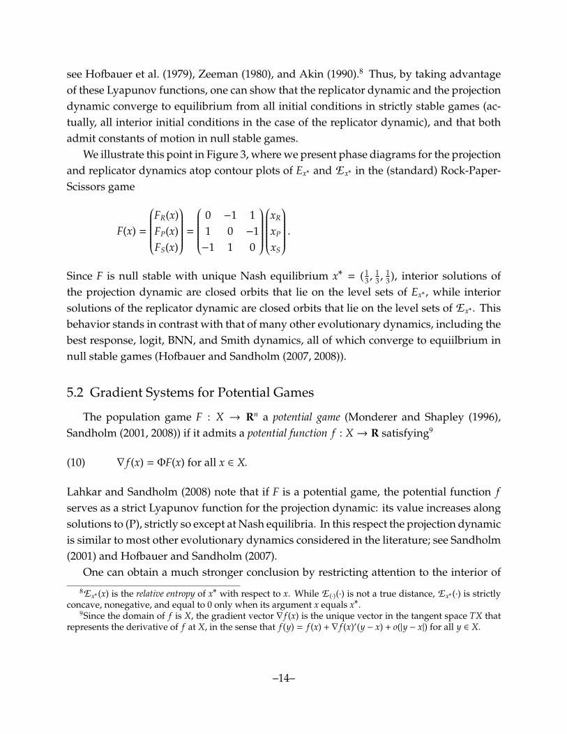
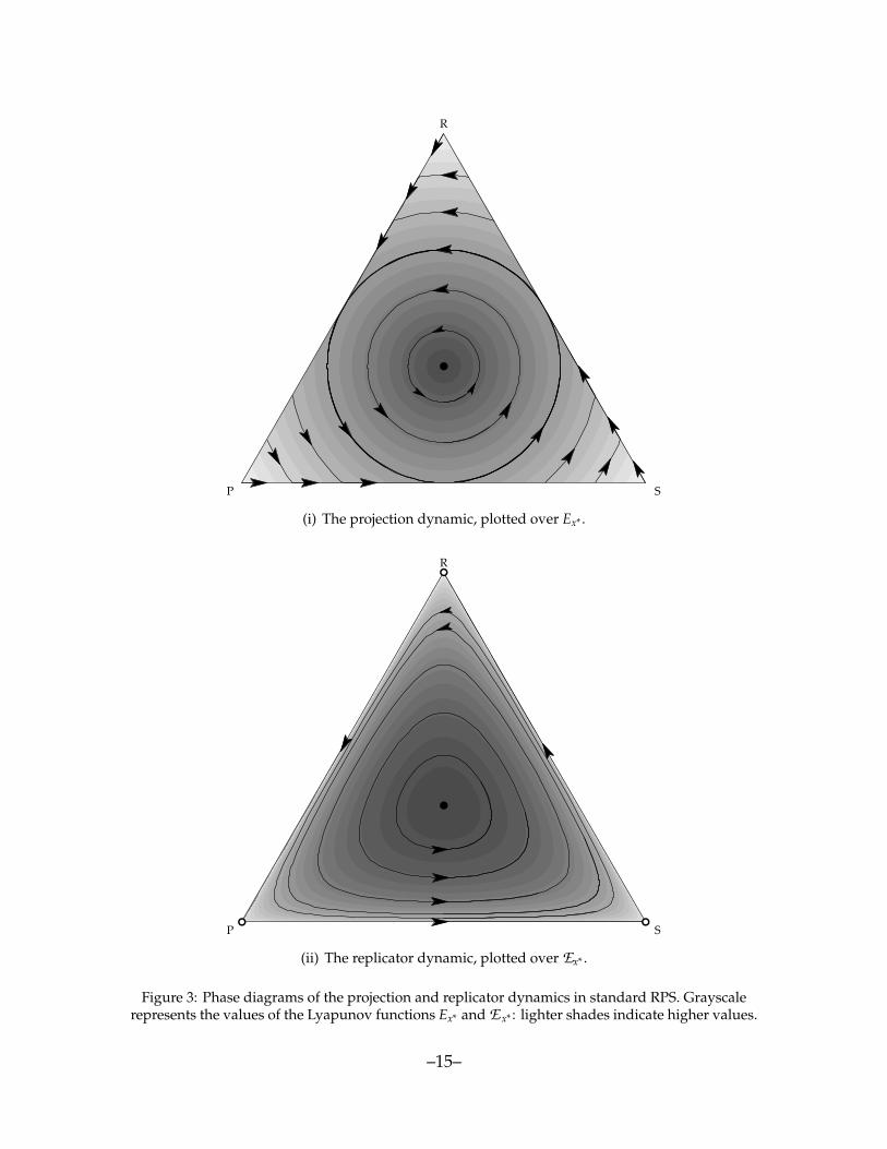
We illustrate this point in Figure 3, where we present phase diagrams for the projectionand replicator dynamics atop contour plots of Ex∗ and E x∗ in the (standard) Rock-Paper-Scissors game

F(x) =

FR(x)FP(x)FS(x)

=

0 −1 11 0 −1−1 1 0

xR

xP

xS

.Since F is null stable with unique Nash equilibrium x∗ = ( 1

3 ,13 ,

13 ), interior solutions of

the projection dynamic are closed orbits that lie on the level sets of Ex∗ , while interiorsolutions of the replicator dynamic are closed orbits that lie on the level sets of E x∗ . Thisbehavior stands in contrast with that of many other evolutionary dynamics, including thebest response, logit, BNN, and Smith dynamics, all of which converge to equiilbrium innull stable games (Hofbauer and Sandholm (2007, 2008)).

5.2 Gradient Systems for Potential Games

The population game F : X → Rn a potential game (Monderer and Shapley (1996),Sandholm (2001, 2008)) if it admits a potential function f : X→ R satisfying9

(10) ∇ f (x) = ΦF(x) for all x ∈ X.

Lahkar and Sandholm (2008) note that if F is a potential game, the potential function fserves as a strict Lyapunov function for the projection dynamic: its value increases alongsolutions to (P), strictly so except at Nash equilibria. In this respect the projection dynamicis similar to most other evolutionary dynamics considered in the literature; see Sandholm(2001) and Hofbauer and Sandholm (2007).

One can obtain a much stronger conclusion by restricting attention to the interior of

8E x∗ (x) is the relative entropy of x∗ with respect to x. While E (·)(·) is not a true distance, E x∗ (·) is strictlyconcave, nonegative, and equal to 0 only when its argument x equals x∗.

9Since the domain of f is X, the gradient vector ∇ f (x) is the unique vector in the tangent space TX thatrepresents the derivative of f at X, in the sense that f (y) = f (x) + ∇ f (x)′(y − x) + o(|y − x|) for all y ∈ X.

–14–

R

P S

(i) The projection dynamic, plotted over Ex∗ .

R

P S

(ii) The replicator dynamic, plotted over Ex∗ .

Figure 3: Phase diagrams of the projection and replicator dynamics in standard RPS. Grayscalerepresents the values of the Lyapunov functions Ex∗ and E x∗ : lighter shades indicate higher values.

–15–

1

2 3

Figure 4: Phase diagram of (P) for coordination game (12). Grayscale represents the value ofpotential: lighter colors indicate higher values.

the simplex. There the projection dynamic is actually the gradient system for f :

(11) x = ∇ f (x) on int(X),

In geometric terms, (11) says that interior solutions to (P) cross the level sets of the forthogonally. We illustrate this point in Figure 4, where we present the phase diagram ofthe projection dynamic in the pure coordination game

(12) F(x) =

F1(x)F2(x)F3(x)

=1 0 00 2 00 0 3

x1

x2

x3

.The contour plot in this figure shows the level sets of the game’s potential function,

f (x) =12

((x1)2 + 2(x2)2 + 3(x3)2

).

Evidently, solutions trajectories of (P) in the interior of the simplex cross the level sets off at right angles.

–16–

Remarkably enough, it is also possible to view the replicator dynamic for F as agradient system for the potential function f . Shahshahani (1979), building on the earlywork of Kimura (1958), showed that the replicator dynamic for a potential game is agradient dynamic after a “change in geometry”—in particular, after the introduction ofan appropriate Riemannian metric on int(X). Subsequently, Akin (1979) (see also Akin(1990)) established that Shahshahani’s (1979) Riemannian manifold is isometric to the setX = {x ∈ Rn

+ :∑

i∈S x 2i = 4}, the portion of the raidus 2 sphere lying in the positive orthant,

endowed with the usual Euclidean metric. It follows that if we use Akin’s (1979) isometryto transport the replicator dynamic for the potential game F to the set X , this transporteddynamic is a gradient system in the usual Euclidean sense. To conclude the paper, weprovide a direct proof of this striking fact, a proof that does not require intermediate stepsthrough differential geometry.

Akin’s (1979) transformation, which we denote by H : int(Rn+)→ int(Rn

+), is defined byHi(x) = 2

√xi. As we noted earlier, H is a diffeomorphism that maps the simplex X onto

the set X . We wish to prove

Theorem 5.1. Let F : X → Rn be a potential game with potential function f : X → R. Supposewe transport the replicator dynamic for F on int(X) to the set int(X ) using the transformationH. Then the resulting dynamic is the (Euclidean) gradient dynamic for the transported potentialfunction φ = f ◦H−1.

Since Hi(x) = 2√

xi, the transformation H makes changes in component xi look largewhen xi itself is small. Therefore, Theorem 5.1 tells us that the replicator dynamic is agradient dynamic on int(X) after a change of variable that makes changes in the use ofrare strategies look important relative to changes in the use of common ones. Intuitively,this reweighting accounts for the fact that under imitative dynamics, both increases anddecreases in the use of rare strategies are necessarily slow.

Proof. We prove Theorem 5.1 in two steps: first, we derive the transported version ofthe replicator dynamic; then we derive the gradient system for the transported version ofthe potential function, and show that it is the same dynamic on X . The following notationwill simplify our calculations: when y ∈ Rn

+ and a ∈ R, we let [ya] ∈ Rn be the vector whoseith component is (yi)a.

We can express the replicator dynamic on X as

x = R(x) = diag(x) (F(x) − 1x′F(x)) =(diag (x) − xx′

)F(x).

–17–

The transported version of this dynamic can be computed as

x = R (x ) = DH(H−1(x ))R(H−1(x )).

In words: given a state x ∈ X , we first find the corresponding state x = H−1(x ) ∈ X anddirection of motion R(x). Since R(x) represents a displacement from state x, we transportit to X by premultiplying it by DH(x), the derivative of H evaluated at x.

Since x = H(x) = 2 [x1/2], the derivative of H at x is given by DH(x) = diag([x−1/2])Using this fact, we derive a primitive expression for R (x ) in terms of x = H−1(x ) = 1

4 [x 2]:

x = R (x )(13)

= DH(x)R(x)

= diag([x−1/2])(diag(x) − xx′)F(x)

=(diag([x1/2]) − [x1/2]x′

)F(x).

Now, we derive the gradient system on X generated byφ = f ◦H−1. To compute∇φ(x ),we need to define an extension of φ to all of Rn

+, compute its gradient, and then project theresult onto the tangent space of X at x . The easiest way to proceed is to let f : int(Rn

+)→ Rbe an arbitrary C1 extension of f , and to define the extension φ : int(Rn

+)→ R by φ = f ◦H−1.Since X is a portion of a sphere centered at the origin, the tangent space of X at x

is the subspace TX (x ) = {z ∈ Rn : x ′z = 0}. The orthogonal projection onto this set isrepresented by the n × n matrix

PTX (x ) = I −1

x ′x xx ′ = I −14

xx ′ = I − [x1/2][x1/2]′.

Also, sinceΦ∇ f (x) = ∇ f (x) = ΦF(x) by construction, it follows that ∇ f (x) = F(x)+ c(x)1 forsome scalar-valued function c : X → R. Therefore, the gradient system on X generatedby φ is

x = ∇φ(x )

= PTX (x )∇φ(x )

= PTX (x )DH−1(x )′∇ f (x)

= PTX (x ) (DH(x)−1)′ (F(x) + c(x)1)

=(I − [x1/2][x1/2]′

)diag([x1/2]) (F(x) + c(x)1)

=(diag([x1/2]) − [x1/2]x′

)(F(x) + c(x)1)

–18–

1

2 3

(i) origin of projection = H( 13 ,

13 ,

13 )

1

2

3

(ii) origin of projection = H( 17 ,

17 ,

57 )

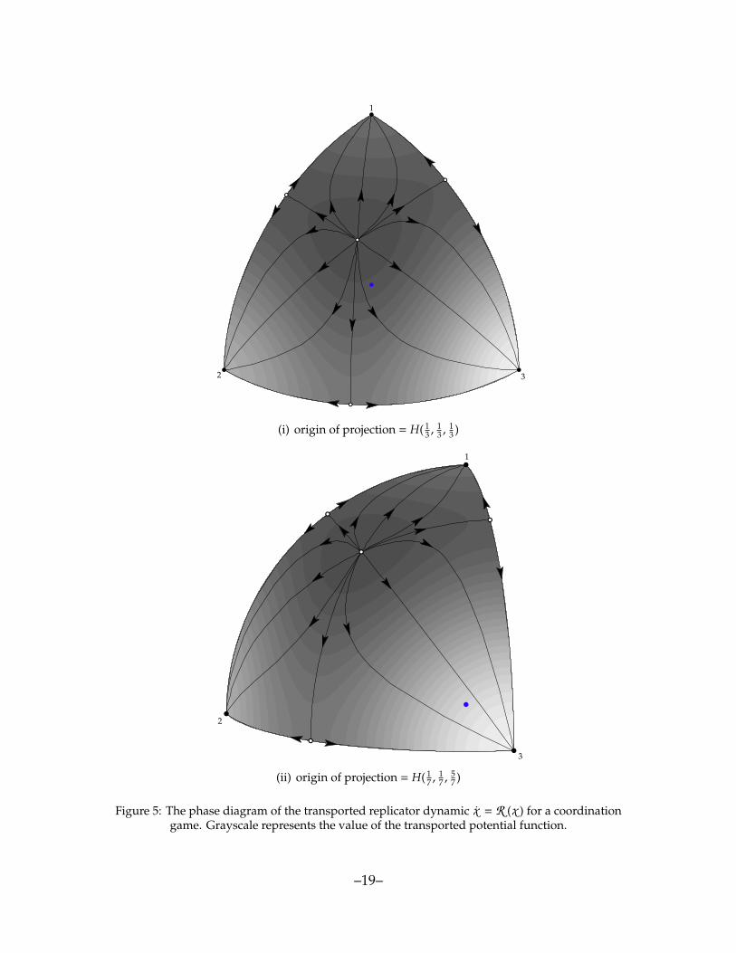
Figure 5: The phase diagram of the transported replicator dynamic x = R (x ) for a coordinationgame. Grayscale represents the value of the transported potential function.

–19–

=(diag([x1/2]) − [x1/2]x′

)F(x).

This agrees with equation (13), completing the proof of the theorem. �

In Figure 5, we illustrate Theorem 5.1 with phase diagrams of the transported replicatordynamic x = R (x ) for the three-strategy coordination game from equation (12). Thesephase diagrams on X are drawn atop contour plots of the transported potential functionφ(x ) = ( f ◦ H−1)(x ) = 1

32 ((x1)4 + 2(x2)4 + 3(x3)4). According to Theorem 5.1, the solutiontrajectories of R should cross the level sets of φ orthogonally.

Looking at Figure 5(i), we find that the crossings look orthogonal at the center of thefigure, but not by the boundaries. This is an artifact of our drawing a portion of the spherein R3 by projecting it orthogonally onto a sheet of paper.10 To check whether the crossingsnear a given state x ∈ X are truly orthogonal, we can minimize the distortion of anglesnear x by making x the origin of the projection.11 We mark the projection origins inFigures 5(i) and Figures 5(ii) with dots; evidently, the crossings are orthogonal near thesepoints.

A. Appendix

The Proof of Theorem 4.1The method used to construct the approximate closed orbit of (P) is described in the

text after the statement of the theorem. Here, we verify that this approximation impliesthe existence of an exact closed orbit of (P). A minor modification of our argument showsthat this orbit absorbs all nearby trajectories in finite time.

Let us review the construction of the approximate closed orbit. We begin by choosingthe initial state ξ0 = ξ = ( 7

15 ,8

15 , 0, 0). The (exact) solution to (P) from ξ initially travelsthrough face RPS in a fashion described by the linear differential equation (3), and so becomputed analytically. The solution exits face RPS into the interior of X when it hits theline on which the payoff to T equals the average of the payoffs to R, P, and S. The exitpoint cannot be determined analytically, but it can be approximated to any desired degreeof accuracy. We call this approximate exit point, which we compute to 16 decimal places,ξ1≈ (.446354, .552864, .000782, 0), and we call the time that the solution to (P) reaches this

point t1≈ .015678.

10For the same reason, latitude and longitude lines in an orthographic projection of the Earth only appearto cross at right angles in the center of the projection, not on the left and right sides.

11The origin of the projection, o ∈ X , is the point where the sphere touches the sheet of paper. If we viewthe projection from any point on the ray that exits the sheet of paper orthogonally from o, then the center ofthe sphere is directly behind o.

–20–

Next, we consider the (exact) solution to (P) from starting from state ξ1. This solutiontravels through int(X) until it reaches face PST. We again compute an approximate exitpoint ξ2, and we let t2 be the total time expended during the first two solution segments.Continuing in this fashion, we compute the approximate exit points ξ3, . . . , ξ7, and thetransition times t3, . . . , t7.

Now for each state ξk, let {xkt }t≥tk be the solution to (P) that starts from state ξk at time

tk. Because solutions to (P) are Lipschitz continuous in their initial conditions (see Lahkarand Sandholm (2008)), we can bound the distance between state x0

t7 , which is the locationof the solution to (P) from state ξ0 = ξ at time t7, and state x7

t7 = ξ7, as follows:

∣∣∣x0t7 − x7

t7

∣∣∣ ≤ 7∑k=1

∣∣∣xk−1t7 − xk

t7

∣∣∣ ≤ 7∑k=1

eK(t7−tk)ε.

Here, K is the Lipschitz coefficient for the payoff vector field F, and ε is an upper boundon the roundoff error introduced when we compute the approximate exit point ξk for thesolution to (P) from state ξk−1.

Since F(x) = Ax is linear, its Lipschitz coefficient is the spectral norm of the payoffmatrix A: that is, the square root of the largest eigenvalue of A′A (see Horn and Johnson(1985)). A computation reveals that the spectral norm of A is approximately 5.718145.Since we compute our approximate exit points to 16 decimal places, our roundoff errorsare no greater than 5×10−17. Thus, since t7

− t1 = 1.049900, we obtain the following boundon the distance between x0

t7 and x7t7 :∣∣∣x0

t7 − x7t7

∣∣∣ ≤ 7(eK(t7−tk)ε

)≈ 7

(e(5.718145)(1.049900)

× (5 × 10−17))≈ 1.416920 × 10−13.

It is easy to verify that any solution to (P) that starts within this distance of state ξ7≈

(.693072, .306928, 0, 0) will hit edge RP between vertex R and state ξ, and so continue on toξ. We therefore conclude that {x0

t }t≥0, the exact solution to (P) starting from state ξ, mustreturn to state ξ. This completes the proof of the theorem. �

References

Akin, E. (1979). The Geometry of Population Genetics. Springer, Berlin.

Akin, E. (1980). Domination or equilibrium. Mathematical Biosciences, 50:239–250.

–21–

Akin, E. (1990). The differential geometry of population genetics and evolutionary games.In Lessard, S., editor, Mathematical and Statistical Developments of Evolutionary Theory,pages 1–93. Kluwer, Dordrecht.

Benaım, M. and Weibull, J. W. (2003). Deterministic approximation of stochastic evolutionin games. Econometrica, 71:873–903.

Berger, U. and Hofbauer, J. (2006). Irrational behavior in the Brown-von Neumann-Nashdynamics. Games and Economic Behavior, 56:1–6.

Bjornerstedt, J. and Weibull, J. W. (1996). Nash equilibrium and evolution by imitation. InArrow, K. J. et al., editors, The Rational Foundations of Economic Behavior, pages 155–181.St. Martin’s Press, New York.

Friedman, D. (1991). Evolutionary games in economics. Econometrica, 59:637–666.

Hofbauer, J. (1995). Imitation dynamics for games. Unpublished manuscript, Universityof Vienna.

Hofbauer, J. and Sandholm, W. H. (2006). Survival of dominated strategies under evo-lutionary dynamics. Unpublished manuscript, University of Vienna and University ofWisconsin.

Hofbauer, J. and Sandholm, W. H. (2007). Evolution in games with randomly disturbedpayoffs. Journal of Economic Theory, 132:47–69.

Hofbauer, J. and Sandholm, W. H. (2008). Stable population games and integrability forevolutionary dynamics. Unpublished manuscript, University of Vienna and Universityof Wisconsin.

Hofbauer, J., Schuster, P., and Sigmund, K. (1979). A note on evolutionarily stable strategiesand game dynamics. Journal of Theoretical Biology, 81:609–612.

Hofbauer, J. and Weibull, J. W. (1996). Evolutionary selection against dominated strategies.Journal of Economic Theory, 71:558–573.

Horn, R. A. and Johnson, C. R. (1985). Matrix Analysis. Cambridge University Press,Cambridge.

Kimura, M. (1958). On the change of population fitness by natural selection. Heredity,12:145–167.

Lahkar, R. and Sandholm, W. H. (2008). The projection dynamic and the geometry ofpopulation games. Games and Economic Behavior, forthcoming.

Monderer, D. and Shapley, L. S. (1996). Potential games. Games and Economic Behavior,14:124–143.

–22–

Nagurney, A. and Zhang, D. (1996). Projected Dynamical Systems and Variational Inequalitieswith Applications. Kluwer, Dordrecht.

Nagurney, A. and Zhang, D. (1997). Projected dynamical systems in the formulation,stability analysis, and computation of fixed demand traffic network equilibria. Trans-portation Science, 31:147–158.

Samuelson, L. and Zhang, J. (1992). Evolutionary stability in asymmetric games. Journalof Economic Theory, 57:363–391.

Sandholm, W. H. (2001). Potential games with continuous player sets. Journal of EconomicTheory, 97:81–108.

Sandholm, W. H. (2003). Evolution and equilibrium under inexact information. Gamesand Economic Behavior, 44:343–378.

Sandholm, W. H. (2008). Potential functions for normal form games and for populationgames. Unpublished manuscript, University of Wisconsin.

Schlag, K. H. (1998). Why imitate, and if so, how? A boundedly rational approach tomulti-armed bandits. Journal of Economic Theory, 78:130–156.

Shahshahani, S. (1979). A new mathematical framework for the study of linkage andselection. Memoirs of the American Mathematical Society, 211.

Taylor, P. D. and Jonker, L. (1978). Evolutionarily stable strategies and game dynamics.Mathematical Biosciences, 40:145–156.

Zeeman, E. C. (1980). Population dynamics from game theory. In Nitecki, Z. and Robinson,C., editors, Global Theory of Dynamical Systems (Evanston, 1979), number 819 in LectureNotes in Mathematics, pages 472–497, Berlin. Springer.

–23–