Embed Size (px)
Citation preview

Maximo Camacho and Danilo Leiva-Leon
Documentos de Trabajo N.º 1728
2017THE PROPAGATION OF INDUSTRIAL BUSINESS CYCLES

THE PROPAGATION OF INDUSTRIAL BUSINESS CYCLES

THE PROPAGATION OF INDUSTRIAL BUSINESS CYCLES (*)
Maximo Camacho
UNIVERSITY OF MURCIA
Danilo Leiva-Leon (**)
BANCO DE ESPAÑA
Documentos de Trabajo. N.º 1728
2017
(*) We are thankful to Gabriel Perez Quiros, the editor and two anonymous referees for their comments. M. Camacho acknowledges the financial support from projects ECO2013-45698-P and ECO2016-76178-P., whose contribution also is there result of the activity carried out under the program Groups of Excellence of the region of Murcia, the Fundación Seneca, Science and Technology Agency of the region of Murcia project 19884/GERM/15. All remaining error sare our responsibility. The views expressed in this paper are those of the authors and do not represent the views of the Banco de España or the Eurosystem. (**) Corresponding Author: ADG Economics and Research, Banco de España, Alcalá 48, Madrid-Spain. E-mail: [email protected].

The Working Paper Series seeks to disseminate original research in economics and fi nance. All papers have been anonymously refereed. By publishing these papers, the Banco de España aims to contribute to economic analysis and, in particular, to knowledge of the Spanish economy and its international environment.
The opinions and analyses in the Working Paper Series are the responsibility of the authors and, therefore, do not necessarily coincide with those of the Banco de España or the Eurosystem.
The Banco de España disseminates its main reports and most of its publications via the Internet at the following website: http://www.bde.es.
Reproduction for educational and non-commercial purposes is permitted provided that the source is acknowledged.
© BANCO DE ESPAÑA, Madrid, 2017
ISSN: 1579-8666 (on line)

Abstract
This paper examines the evolution of the distribution of industry-specifi c business cycle
linkages, which are modelled through a multivariate Markov-switching model and estimated
by Gibbs sampling. Using non parametric density estimation approaches, we fi nd that the
number and location of modes in the distribution of industrial dissimilarities change over
the business cycle. There is a relatively stable trimodal pattern during expansionary and
recessionary phases characterized by highly, moderately and lowly synchronized industries.
However, during phase changes, the density mass spreads from moderately synchronized
industries to lowly synchronized industries. This agrees with a sequential transmission
of the industrial business cycle dynamics.
Keywords: business bycles, output growth, time series.
JEL classifi cation: E32, C22, E27.

Resumen
En este artículo se examina la evolución de la distribución de los vínculos de ciclos
económicos a nivel de industria, los cuales son modelados con procesos markovianos
multivariados y estimados por el muestreo de Gibbs. Utilizando técnicas no paramétricas,
se encuentra que el número y la ubicación de las modas de la distribución de disimilitudes
industriales cambian a lo largo del ciclo económico. En particular, existe un patrón trimodal
relativamente estable durante las fases expansivas y recesivas, caracterizadas por industrias
con sincronía alta, moderada y baja. Sin embargo, durante los cambios de fase del ciclo
económico, la masa de densidad se desplaza desde las industrias moderadamente
sincronizadas hasta las industrias poco sincronizadas. Esto concuerda con una transmisión
secuencial de los choques que afectan a los ciclos económicos industriales.
Palabras clave: ciclos económicos, actividad industrial, dinámicas no lineales.
Códigos JEL: E32, C22, E27.
BANCO DE ESPAÑA 7 DOCUMENTO DE TRABAJO N.º 1728
1 Introduction
In practice, people do not know the state of the business cycle, which is especially uncertain
around turning points. This could be because “the state of the economy” depends on the behav-
iour of many interdependent industries that do not necessarily all “boom” when the aggregate
economy is prosperous or “bust” when the economy is in recession. Accordingly, although the
aggregate business cycle could be described at a macro level as a series of distinct recession
and expansion phases, it could never be understood at that level. Although recessions are
not all alike, some lessons can be learned regarding their propagation when tracking the micro
foundations of cycles through a variety of interconnected market dynamics at industry levels.
There is an increasing interest in understanding business cycles at a disaggregate level. Long
and Plosser (1983) was amongst the first works to highlight the potential role of sectors in the
transmission of business cycle shocks. Horvath (1998, 2000), Dupor (1999), and Carvalho (2008)
took into account sectoral linkages across sectors. Long and Plosser (1987), Forni and Reichlin
(1998) and Shea (2002) assessed the relative contributions of aggregate and sector-specific shocks
to aggregate variability. Recently, Karadimitropoulou and Leon-Ledesma (2013) extended this
analysis to an international setting, showing that industry-specific factors account for a large
proportion of the variance of value added growth for most of the G7 countries.
Four strands of the existing literature are of special interest for the analysis developed in
this paper. First, Gabaix (2011) and Acemoglu et al. (2012) postulate that when there are
significant asymmetries in the roles that industries play as suppliers to others, idiosyncratic firm-
level shocks can explain an important part of aggregate movements. Foerster, Sarte and Watson
(2011) show that the role of sectoral shocks increased considerably after the Great Moderation.
Second, the sharp downturn in the economy experienced in 2008 and the subsequent jobless
recovery increased concerns for security for asset holders (Malmendier and Nagel, 2011) and
for people seeking work (Urquhart, 1981). In this context, understanding the transmission
of shocks across industries appeared to be a necessary condition for the optimality of these
economic agents’ decisions. Third, although the business cycle analysis has largely focused on
national-level phases, there is a growing interest in state-level data (Owyang, Piger and Wall,
2005, and Hamilton and Owyang, 2012) and in city-level data (Owyang et al. 2008). The state-
level analyses find that the disparities in regional business cycles can partially be attributed
to differences in the industrial composition of the regions and the city-level analyses find that
the low-phase growth is related only to the relative importance of manufacturing. Fourth, little
attention has been paid to analyzing synchronization of business cycle dynamics at the industry
level. Without being exhaustive, some examples include Christiano and Fitzgerald (1998), who
BANCO DE ESPAÑA 8 DOCUMENTO DE TRABAJO N.º 1728
gauge the extent of co-movement across a range of disaggregated sector categories and the total
by computing the square of the correlation between their business cycle components in hours
worked, which are the outcome of band-pass filters. Carlino and DeFina (2004) focus on the
analysis of growth cycles by examining the pairwise correlation between the sectorial cycles in
band-pass filtered employment. Recently, Goodman and Mance (2011) analyze the per cent
change in industry employment data during recessions, as determined by the National Bureau
of Economic Research (NBER).
In line with these contributions, the main purpose of this paper is to understand (1) which
industries manifest the first signs of the phase changes, (2) how the interconnections across
industries lead to cascade effects that propagate the idiosyncratic shocks across sectors, and
(3) the evolution of the cyclical similarities among industries over the aggregate business cycle.
Our analysis contributes to several strands in the existing literature. First, we complement the
analyses of Gabaix (2011), Acemoglu et al. (2012) and Foerster et al. (2011) by focusing on
the transmission of shocks over distinct business cycle phases. Second, our analysis provides
assessments of the industries that are less sensitive to the aggregate cycle in bad times, which
may represent useful information for investors and workers. Third, our analysis complements the
business cycle analyses in state-level and city-level data by examining the business cycle at the
industry level. Fourth, one important drawback of Christiano and Fitzgerald (1998), Carlino
and DeFina (2004) and Goodman and Mance (2011) is that they rely on static measures of
synchronization, such that changes over time can only be captured by splitting the samples into
sub-periods. The problem with this approach is that it provides pictures of the cycle linkages
that rely on specific date breaks, the location of which is sometimes controversial.
To overcome this drawback, we adapt the framework of Leiva-Leon (2016) to examine the
evolution of the time-varying dynamic interactions across the industry cycles. In particular, each
of the industrial cycles is viewed as a continuous-valued Markov-switching variable whose transi-
tion between two distinct phases defines the states of its business cycles. The synchronization of
two industries in a bivariate specification is viewed as a time-varying combination between two
extreme cases: (i) two independent Markov processes, which indicate completely independent
industries; and (ii) a unique Markov process shared by both industries, which indicates perfect
synchronization. The shifts between these extreme regimes is governed by the outcome of an
unobserved Markov chain.
By means of purely statistical techniques, such as nonparametric density estimation and
bootstrap multimodality tests, the number of modes in the time-varying distributions of pairwise
business cycle dissimilarities is tested. This is useful to uncover distinct business cycle dynamics
BANCO DE ESPAÑA 9 DOCUMENTO DE TRABAJO N.º 1728
for different population subgroups of industries and to assess how these subgroups evolve across
the distinct phases of the business cycle. Also, multi-dimensional scaling techniques are used to
understand the formation of these subgroups and their intra-distribution transitional dynamics.
We report two major findings. First, we find that, at a micro level, the U.S. business cycle
is a more elusive phenomenon than we would have expected at the macro level. While some
industries seem to “stick together” and show business cycle experiences that are similar to those
of the nation, there are many that do not. Goods-producing industries, complementary busi-
nesses, and wholesale and retail industries are among the first to fall at the onset of recessions.
However, durable goods industries, professional and technical services, and industries providing
transportation and warehousing and storage for goods do not experience job cuts until some
time after the beginning of recessions. In addition, businesses engaged in providing education
and training, health care and social assistance and industries providing utility services and pub-
lic goods are less sensitive to national recessions, especially in the 2001 recession. These results
agree with Peterson and Strongin (1996), who examine the cyclicality of industries, finding that
durable goods industries are three times more cyclical than non-durable goods industries.
Second, we detect a thought-provoking recurrent business cycle pattern. Over the past three
decades, a salient characteristic of the U.S. cycle dynamics is that the distribution of business
cycle dissimilarities across industries shifts over time. During expansions and recessions, the
distribution is characterized by three clusters of highly, moderately and lowly synchronized in-
dustries, yielding a trimodal distribution. However, during periods of shifts in business cycle
phases or turning points, the moderately synchronized industries enjoy downward synchroniza-
tion mobility and shift over to the lowly synchronized cluster, yielding a bimodal distribution.
Once the transitions end, the trend is reversed as the economy stabilizes in the new business
cycle phase.
The structure of this paper is organized as follows. Section 2 describes the framework used to
compute inferences on the industrial business cycle dynamics. Section 3 presents the empirical
results. Section 4 concludes and proposes some lines for future research.
2 Assessing industrial business cycles
Two things are required to study co-movement across industries over the business cycle: a
measure of economic activity in the industries and a precise definition of their business cycles.
In this paper, the economic activity at date t in a given sector is measured by the annual growth
rates of total employees in the sector. The definition of business cycles relies on the recognized
empirical fact that although series on employment present trends, they are not monotonic curves,

BANCO DE ESPAÑA 10 DOCUMENTO DE TRABAJO N.º 1728
but rather exhibit sequences of upturns and downturns. During periods known as recessions,
the value of employment growth rates are usually lower (and sometimes negative) than during
periods of expansion. A natural approach to model this particular non-linear dynamic behaviour
is the regime-switching model proposed by Hamilton (1989).
2.1 Univariate model
Following Hamilton (1989), we assume that the switching mechanism of the k-th sector’s em-
ployment growth at time t, yk,t, is controlled by an unobservable state variable, sk,t. Owyang,
Piger, and Wall (2005) specify a simple switching model that captures this non-linear dynamic:
yk,t = μsk,t + εk,t, (1)
where the growth rate of employment in sector k at date t has the mean μsk,t = μk0 + μk1sk,t,
which is allowed to switch between two distinct regimes. At time t, one can label sk,t = 0 as
expansions and sk,t = 1 as recessions. Deviations from this mean growth rate are created by
εk,t, which is an i.i.d. Gaussian stochastic disturbance with a mean of zero and variance σ2k.
Therefore, employment is expected to exhibit high (usually positive) growth rates in expansions
and low (usually negative) growth rates in recessions. The variable sk,t is assumed to evolve
according to a first-order Markov chain, whose transition probabilities are defined by
p (sk,t = jk|sk,t−1 = ik, sk,t−2 = rk, ..., yk,t−1) = p (sk,t = jk|sk,t−1 = ik) = pkij , (2)
where i, j = 0, 1, and yk,t = (yk,t, , yk,t−1, ....) .
2.2 Bivariate model
Although univariate Markov-switching models provide information about the timing of regime
changes, they are inappropriate for drawing inferences about the synchronization of business
cycles. Camacho and Perez Quiros (2006) show that the business cycle analyses based on
univariate processes are biased to show relatively low values of business cycle synchronization.
Therefore, using univariate models to examine the business cycle interactions across industries
would be particularly inappropriate for industries that exhibit highly synchronized cycles.
Phillips (1991) shows that the univariate model can be slightly modified to examine the
business cycle transmission in a two-sector setup. Let us assume that we are interested in
measuring the degree of business cycle synchronization between two industries, a and b. In
this case, their employment growths are driven by two (possibly dependent) Markov-switching
processes, sa,t and sb,t, which share the statistical properties of the previous latent variable sk,t.
BANCO DE ESPAÑA 11 DOCUMENTO DE TRABAJO N.º 1728
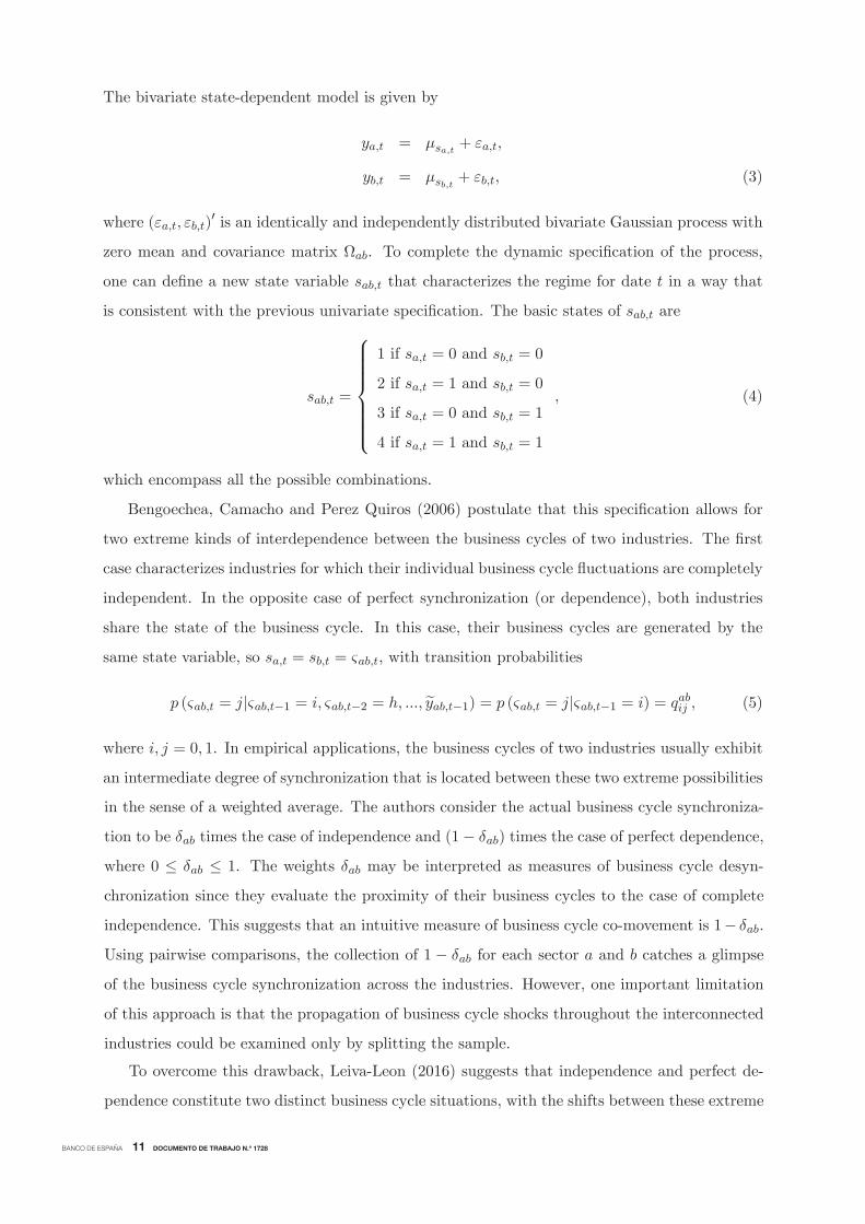
The bivariate state-dependent model is given by
ya,t = μsa,t + εa,t,
yb,t = μsb,t + εb,t, (3)
where (εa,t, εb,t) is an identically and independently distributed bivariate Gaussian process with
zero mean and covariance matrix Ωab. To complete the dynamic specification of the process,
one can define a new state variable sab,t that characterizes the regime for date t in a way that
is consistent with the previous univariate specification. The basic states of sab,t are
sab,t =
⎧⎪⎪⎪⎪⎪⎪⎨⎪⎪⎪⎪⎪⎪⎩
1 if sa,t = 0 and sb,t = 0
2 if sa,t = 1 and sb,t = 0
3 if sa,t = 0 and sb,t = 1
4 if sa,t = 1 and sb,t = 1
, (4)
which encompass all the possible combinations.
Bengoechea, Camacho and Perez Quiros (2006) postulate that this specification allows for
two extreme kinds of interdependence between the business cycles of two industries. The first
case characterizes industries for which their individual business cycle fluctuations are completely
independent. In the opposite case of perfect synchronization (or dependence), both industries
share the state of the business cycle. In this case, their business cycles are generated by the
same state variable, so sa,t = sb,t = ςab,t, with transition probabilities
p (ςab,t = j|ςab,t−1 = i, ςab,t−2 = h, ..., yab,t−1) = p (ςab,t = j|ςab,t−1 = i) = qabij , (5)
where i, j = 0, 1. In empirical applications, the business cycles of two industries usually exhibit
an intermediate degree of synchronization that is located between these two extreme possibilities
in the sense of a weighted average. The authors consider the actual business cycle synchroniza-
tion to be δab times the case of independence and (1− δab) times the case of perfect dependence,
where 0 ≤ δab ≤ 1. The weights δab may be interpreted as measures of business cycle desyn-
chronization since they evaluate the proximity of their business cycles to the case of complete
independence. This suggests that an intuitive measure of business cycle co-movement is 1− δab.
Using pairwise comparisons, the collection of 1 − δab for each sector a and b catches a glimpse
of the business cycle synchronization across the industries. However, one important limitation
of this approach is that the propagation of business cycle shocks throughout the interconnected
industries could be examined only by splitting the sample.
To overcome this drawback, Leiva-Leon (2016) suggests that independence and perfect de-
pendence constitute two distinct business cycle situations, with the shifts between these extreme

BANCO DE ESPAÑA 12 DOCUMENTO DE TRABAJO N.º 1728
where i, j = 0, 1. It is convenient to define a new state variable that governs the individual
business cycles and their degree of synchronization,
s∗ab,t =
⎧⎪⎪⎪⎪⎪⎪⎪⎪⎪⎪⎪⎪⎪⎪⎪⎪⎪⎪⎪⎨⎪⎪⎪⎪⎪⎪⎪⎪⎪⎪⎪⎪⎪⎪⎪⎪⎪⎪⎪⎩
1 if sa,t = 0, sb,t = 0, and vab,t = 0
2 if sa,t = 1, sb,t = 0, and vab,t = 0
3 if sa,t = 0, sb,t = 1, and vab,t = 0
4 if sa,t = 1, sb,t = 1, and vab,t = 0
5 if sa,t = 0, sb,t = 0, and vab,t = 1
6 if sa,t = 1, sb,t = 0, and vab,t = 1
7 if sa,t = 0, sb,t = 1, and vab,t = 1
8 if sa,t = 1, sb,t = 1, and vab,t = 1
, (8)
which also follows a first-order Markov chain.1 Using an extended version of the procedure
described in Hamilton (1989), inferences on the business cycle states are calculated as a by-
product of an algorithm, which is similar in spirit to a Kalman filter. Briefly, the procedure is
based on the iterative application of the following two steps.2
1The probabilities of occurrence of states 6 and 7 are zero by definition.2We focus on the case of industries switching between two regimes. In principle, the analysis can be extended,
allowing for more regimes. However, the analysis of synchronization would become cumbersome and the output
would be less easy to interpret.
regimes governed by the outcome of an unobserved first-order Markov chain, vab,t, whose tran-
sition probabilities are given by
p (vab,t = j|vab,t−1 = i, vab,t−2 = r, ..., yab,t−1) = p (vab,t = j|vab,t−1 = i) = pabij , (6)
where i, j = 0, 1, and yab,t = (ya,t, , ya,t−1, ...., yb,t, yb,t−1, ....) . Here, the state variable vab,t
reflects the actual state of the business cycle synchronization between industries a and b at time
t. In what follows, vab,t = 0 indicates that industries a and b exhibit independent cycles, while
vab,t = 1 indicates that their cycles are fully synchronized (or perfectly dependent). Accordingly,
p (vab,t = 0) measures the probability of independent cycles. Within this framework, one can
easily examine the evolution of the intersectoral business cycle linkages by collecting p (vab,t = 0)
for all a, b and t.
2.3 Inferences
We collect the parameters that fully characterize the model in a vector
θ = (μa0,μa1,μb0,μb1,Ωab, paij , p
bij , q
abij , p
abij ) , (7)
BANCO DE ESPAÑA 13 DOCUMENTO DE TRABAJO N.º 1728
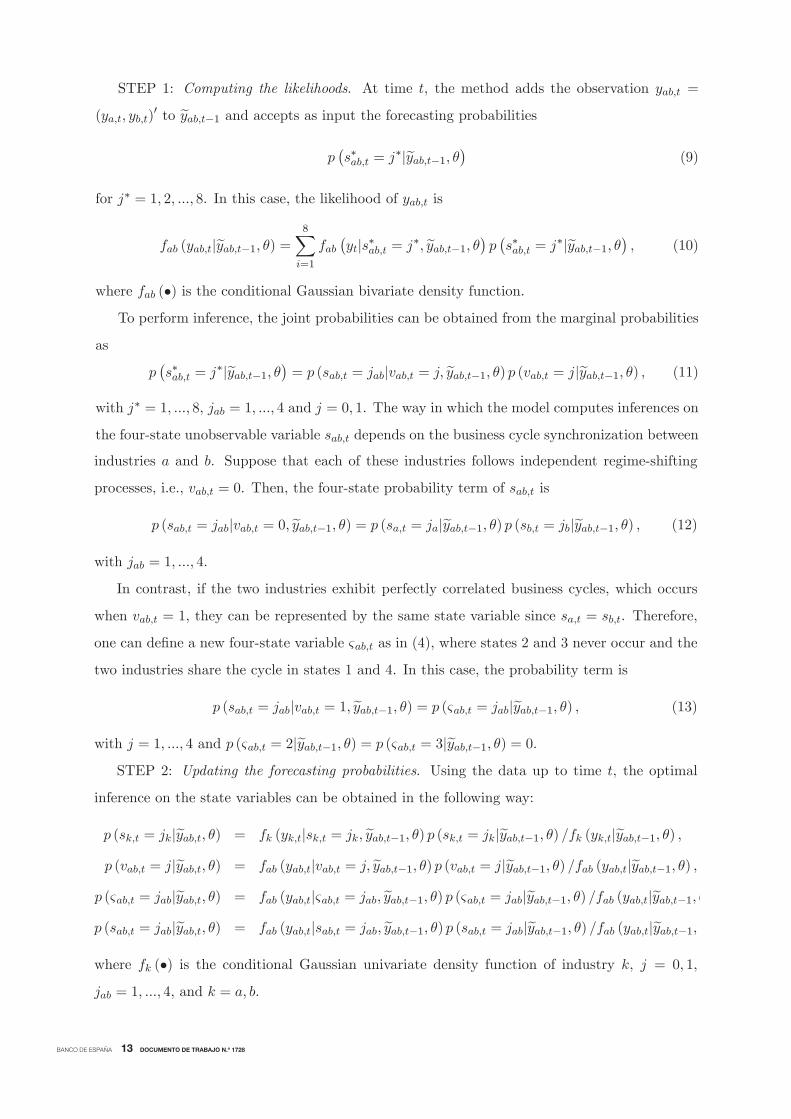
STEP 1: Computing the likelihoods. At time t, the method adds the observation yab,t =
(ya,t, yb,t) to yab,t−1 and accepts as input the forecasting probabilities
p s∗ab,t = j∗|yab,t−1, θ (9)
for j∗ = 1, 2, ..., 8. In this case, the likelihood of yab,t is
fab (yab,t|yab,t−1, θ) =8
i=1
fab yt|s∗ab,t = j∗, yab,t−1, θ p s∗ab,t = j∗|yab,t−1, θ , (10)
where fab (•) is the conditional Gaussian bivariate density function.To perform inference, the joint probabilities can be obtained from the marginal probabilities
as
p s∗ab,t = j∗|yab,t−1, θ = p (sab,t = jab|vab,t = j, yab,t−1, θ) p (vab,t = j|yab,t−1, θ) , (11)
with j∗ = 1, ..., 8, jab = 1, ..., 4 and j = 0, 1. The way in which the model computes inferences on
the four-state unobservable variable sab,t depends on the business cycle synchronization between
industries a and b. Suppose that each of these industries follows independent regime-shifting
processes, i.e., vab,t = 0. Then, the four-state probability term of sab,t is
p (sab,t = jab|vab,t = 0, yab,t−1, θ) = p (sa,t = ja|yab,t−1, θ) p (sb,t = jb|yab,t−1, θ) , (12)
with jab = 1, ..., 4.
In contrast, if the two industries exhibit perfectly correlated business cycles, which occurs
when vab,t = 1, they can be represented by the same state variable since sa,t = sb,t. Therefore,
one can define a new four-state variable ςab,t as in (4), where states 2 and 3 never occur and the
two industries share the cycle in states 1 and 4. In this case, the probability term is
p (sab,t = jab|vab,t = 1, yab,t−1, θ) = p (ςab,t = jab|yab,t−1, θ) , (13)
with j = 1, ..., 4 and p (ςab,t = 2|yab,t−1, θ) = p (ςab,t = 3|yab,t−1, θ) = 0.STEP 2: Updating the forecasting probabilities. Using the data up to time t, the optimal
inference on the state variables can be obtained in the following way:
p (sk,t = jk|yab,t, θ) = fk (yk,t|sk,t = jk, yab,t−1, θ) p (sk,t = jk|yab,t−1, θ) /fk (yk,t|yab,t−1, θ) ,p (vab,t = j|yab,t, θ) = fab (yab,t|vab,t = j, yab,t−1, θ) p (vab,t = j|yab,t−1, θ) /fab (yab,t|yab,t−1, θ) ,p (ςab,t = jab|yab,t, θ) = fab (yab,t|ςab,t = jab, yab,t−1, θ) p (ςab,t = jab|yab,t−1, θ) /fab (yab,t|yab,t−1, θp (sab,t = jab|yab,t, θ) = fab (yab,t|sab,t = jab, yab,t−1, θ) p (sab,t = jab|yab,t−1, θ) /fab (yab,t|yab,t−1, θ
where fk (•) is the conditional Gaussian univariate density function of industry k, j = 0, 1,
jab = 1, ..., 4, and k = a, b.
BANCO DE ESPAÑA 14 DOCUMENTO DE TRABAJO N.º 1728
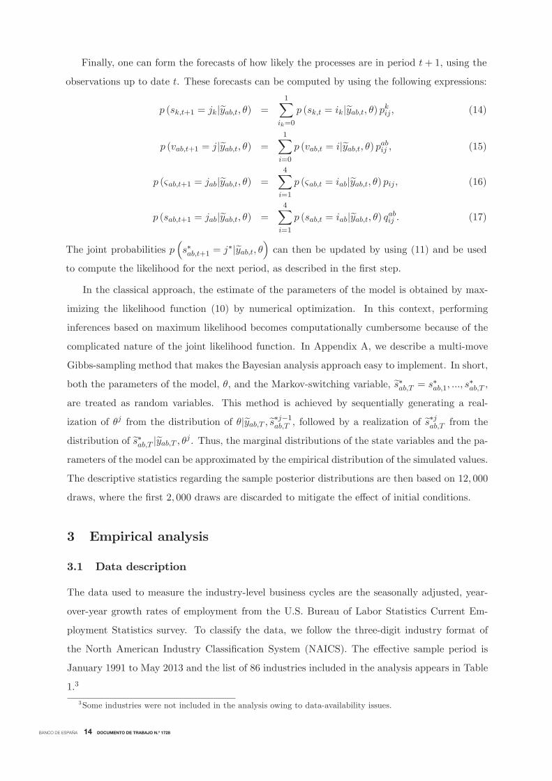
Finally, one can form the forecasts of how likely the processes are in period t+ 1, using the
observations up to date t. These forecasts can be computed by using the following expressions:
p (sk,t+1 = jk|yab,t, θ) =
1
ik=0
p (sk,t = ik|yab,t, θ) pkij , (14)
p (vab,t+1 = j|yab,t, θ) =
1
i=0
p (vab,t = i|yab,t, θ) pabij , (15)
p (ςab,t+1 = jab|yab,t, θ) =4
i=1
p (ςab,t = iab|yab,t, θ) pij , (16)
p (sab,t+1 = jab|yab,t, θ) =
4
i=1
p (sab,t = iab|yab,t, θ) qabij . (17)
The joint probabilities p s∗ab,t+1 = j∗|yab,t, θ can then be updated by using (11) and be used
to compute the likelihood for the next period, as described in the first step.
3Some industries were not included in the analysis owing to data-availability issues.
In the classical approach, the estimate of the parameters of the model is obtained by max-
imizing the likelihood function (10) by numerical optimization. In this context, performing
inferences based on maximum likelihood becomes computationally cumbersome because of the
complicated nature of the joint likelihood function. In Appendix A, we describe a multi-move
Gibbs-sampling method that makes the Bayesian analysis approach easy to implement. In short,
both the parameters of the model, θ, and the Markov-switching variable, s∗ab,T = s∗ab,1, ..., s
∗ab,T ,
are treated as random variables. This method is achieved by sequentially generating a real-
ization of θj from the distribution of θ|yab,T , s∗j−1ab,T , followed by a realization of s∗jab,T from the
distribution of s∗ab,T |yab,T , θj . Thus, the marginal distributions of the state variables and the pa-rameters of the model can be approximated by the empirical distribution of the simulated values.
The descriptive statistics regarding the sample posterior distributions are then based on 12, 000
draws, where the first 2, 000 draws are discarded to mitigate the effect of initial conditions.
3 Empirical analysis
3.1 Data description
The data used to measure the industry-level business cycles are the seasonally adjusted, year-
over-year growth rates of employment from the U.S. Bureau of Labor Statistics Current Em-
ployment Statistics survey. To classify the data, we follow the three-digit industry format of
the North American Industry Classification System (NAICS). The effective sample period is
January 1991 to May 2013 and the list of 86 industries included in the analysis appears in Table
1.3
BANCO DE ESPAÑA 15 DOCUMENTO DE TRABAJO N.º 1728
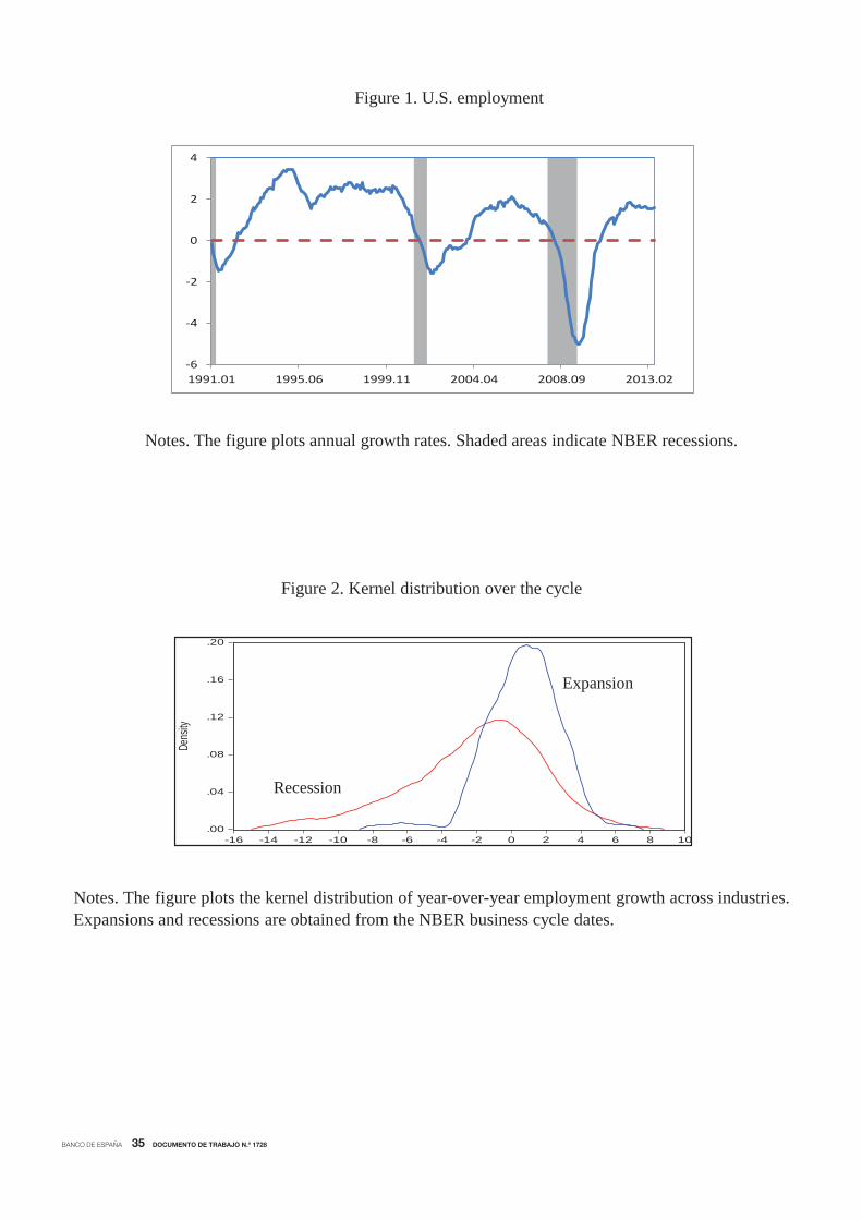
Figure 1 plots the annual growth rates of U.S. unemployment since January 1991, where the
dates of economic recessions, as determined by the NBER, are indicated with shaded regions.
Although employment grows 0.94% during this sample period, the average growth rate in re-
cessions is −1.22%, rising to 1.20% in expansions, which agrees with the well-known procyclical
behaviour of employment at a macro level. In addition, this figure shows that the changes in
employment usually occur a few periods after the changes in the economy as a whole.
However, the picture of employment showing micro data is much more complicated. Ac-
cording to the within-phases averages shown in Table 1, employment growth varied a great deal
across industries over the sample period. Undoubtedly, not all of the industries boom when the
aggregate economy is prosperous and bust when the economy is in recession in a synchronous
manner. For example, 31 out of the 86 three-digit industries, mostly related to agriculture and
manufacturing, exhibit negative average growth rates over the sample. Filardo (1997) postulates
that this might be related to the increasing shift from goods production to services. In addition,
agriculture, manufacturing and construction are all among those industries that contract the
fastest during recessions. The cross-industry differences in growth rates during expansions are
also large, with agriculture, mining and manufacturing industries even losing employees (Barker,
2011).
Figure 2 plots the nonparametric Gaussian kernel estimates of the densities of industrial
employment growth in the NBER recessions and in the NBER expansions. As in the aggregate,
the mean of the recession distribution is negative while the mean of the expansion distribution
is positive. However, there is a large region of considerable overlapping between these two
distributions. This indicates that there are many industries for which employment is falling
rather than rising during a national expansion while others are rising rather than falling during
a national recession. According to this analysis, it seems evident that understanding the business
cycles is more complicated than simply analyzing the cycles at the aggregate level.
3.2 Univariate analysis
We first conduct an analysis of each industry individually to examine the periods of advance
or delay with which the business cycle co-movements might appear. Accordingly, we fit a
univariate model like (1) for each of the identified industries and compute the corresponding
filtered probabilities of low-mean states, which appear in the choropleth maps displayed in
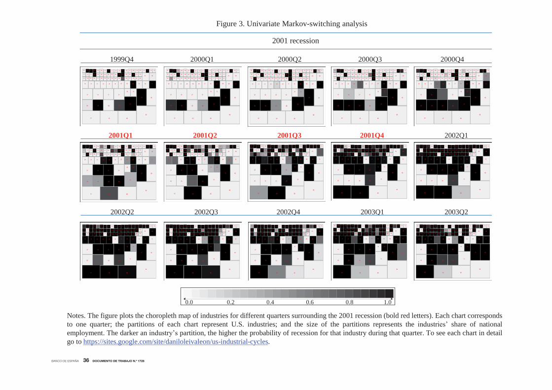
Figures 3 and 4.4 The charts are divided into rectangles that show the relative size of employment
in each of the 86 industries in the total.5 Light colours indicate low evidence of recession, while
the darker the shade, the stronger the statistical confidence that the indicated industry was in

BANCO DE ESPAÑA 16 DOCUMENTO DE TRABAJO N.º 1728
recession at that time. As one moves to the right, the charts show how the business inferences
vary in each quarter, from pre-recession to recession and to the first stages of recovery, as dated
by the NBER.
Several conclusions emerge from the analysis of these choropleth charts. First, recessions are
marked by widespread contractions in many sectors of the economy. Second, goods-producing
4To facilitate the exposition, the monthly figures have been converted to quarterly by averaging over the
respective quarter. The monthly analysis, available upon request, reveals qualitatively similar results.5To simplify the charts, we use the average relative size of industries over the sample period.
industries, complementary businesses, and wholesale and retail industries are among the first
to fall at the onset of recessions. However, durable goods industries, professional and technical
services, businesses that operate facilities or that provide services to meet varied cultural, en-
tertainment and recreational interests, and industries providing transportation and warehousing
and storage for goods do not experience job cuts until some time after the beginning of re-
cessions. Third, businesses engaged in providing education and training, health care and social
assistance and industries providing utility services and public goods are less sensitive to national
recessions, especially to the 2001 recession. Fourth, the synchronization appears to be weaker in
the 2001 recession than in the 2008 recession, which seems to be a more economy-wide recession.
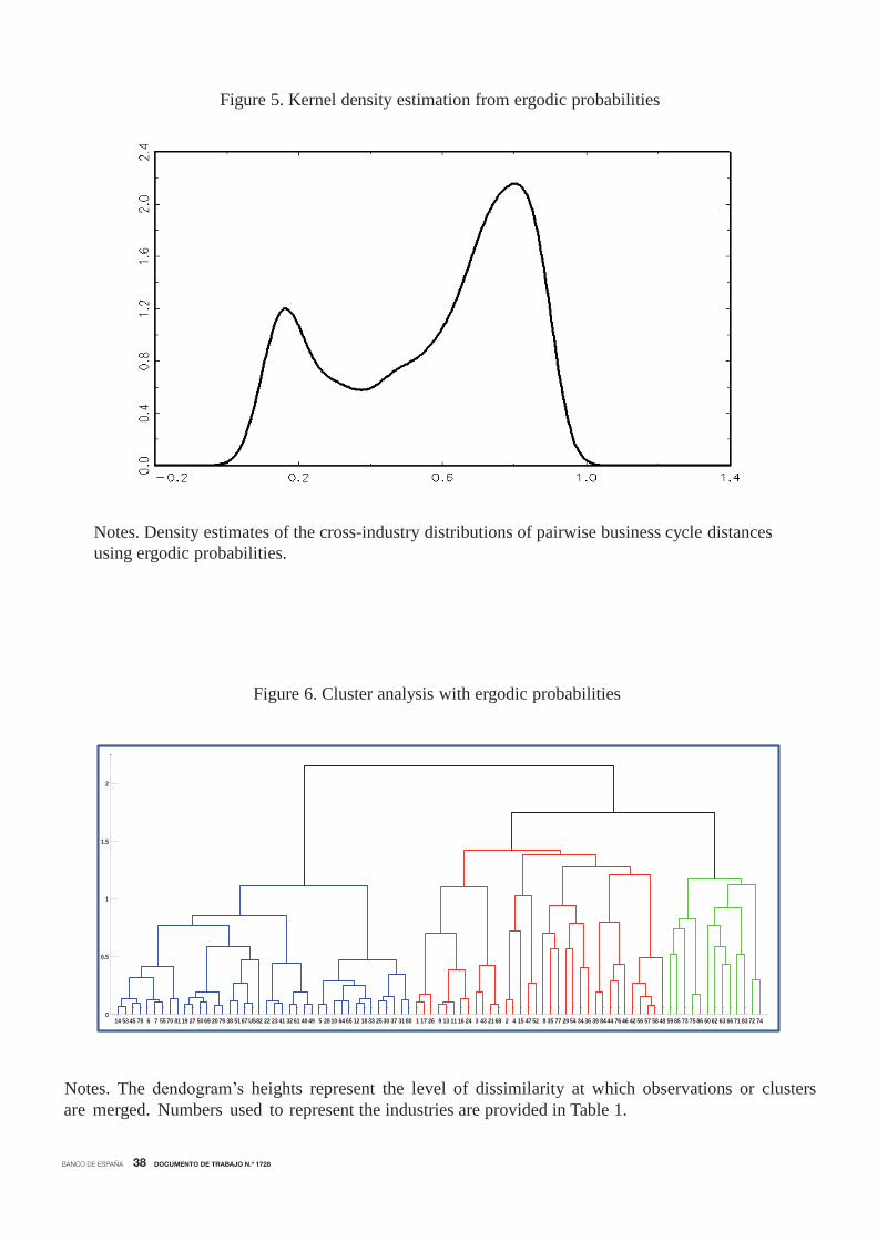
3.3 Ergodic linkages
A glimpse of the business cycle linkages across the industries over the sample can be obtained
by collecting the pairwise ergodic probabilities of the Markov chain that governs the strength of
business cycle synchronization, vab,t, for all industries a, b. Therefore, we begin by calculating
the ergodic probability of being perfectly synchronized, πab1 , and the ergodic probability of facing
independent cycles, πab0 , as follows:
πab0 = 1− pab11 / 2− pab00 − pab11 , (18)
πab1 = 1− pab00 / 2− pab00 − pab11 . (19)
Since the ergodic probabilities can be viewed as the unconditional probability of each of the
different states, the matrix of ergodic synchronizations provides insights on the unconditional
business cycle linkages across the industries. In this section, we focus on the analysis of the
business cycle distances, πab0 .
Although this approach is appealing, a difficulty with it is that there are many such measures.
With a set of N industries, there are η = N (N − 1) /2 different possible business cycle distances.It is therefore a challenge to organize and present the results in a coherent way. To overcome
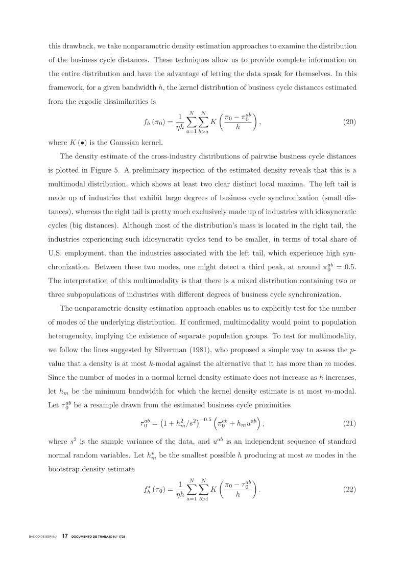
BANCO DE ESPAÑA 17 DOCUMENTO DE TRABAJO N.º 1728
this drawback, we take nonparametric density estimation approaches to examine the distribution
of the business cycle distances. These techniques allow us to provide complete information on
the entire distribution and have the advantage of letting the data speak for themselves. In this
framework, for a given bandwidth h, the kernel distribution of business cycle distances estimated
from the ergodic dissimilarities is
fh (π0) =1
ηh
N
a=1
N
b>a
Kπ0 − πab0
h, (20)
where K (•) is the Gaussian kernel.The density estimate of the cross-industry distributions of pairwise business cycle distances
is plotted in Figure 5. A preliminary inspection of the estimated density reveals that this is a
multimodal distribution, which shows at least two clear distinct local maxima. The left tail is
made up of industries that exhibit large degrees of business cycle synchronization (small dis-
tances), whereas the right tail is pretty much exclusively made up of industries with idiosyncratic
cycles (big distances). Although most of the distribution’s mass is located in the right tail, the
industries experiencing such idiosyncratic cycles tend to be smaller, in terms of total share of
U.S. employment, than the industries associated with the left tail, which experience high syn-
chronization. Between these two modes, one might detect a third peak, at around πab0 = 0.5.
The interpretation of this multimodality is that there is a mixed distribution containing two or
three subpopulations of industries with different degrees of business cycle synchronization.
The nonparametric density estimation approach enables us to explicitly test for the number
of modes of the underlying distribution. If confirmed, multimodality would point to population
heterogeneity, implying the existence of separate population groups. To test for multimodality,
we follow the lines suggested by Silverman (1981), who proposed a simple way to assess the p-
value that a density is at most k-modal against the alternative that it has more than m modes.
Since the number of modes in a normal kernel density estimate does not increase as h increases,
let hm be the minimum bandwidth for which the kernel density estimate is at most m-modal.
Let τab0 be a resample drawn from the estimated business cycle proximities
τab0 = 1 + h2m/s2 −0.5
πab0 + hmuab , (21)
where s2 is the sample variance of the data, and uab is an independent sequence of standard
normal random variables. Let h∗m be the smallest possible h producing at most m modes in the
bootstrap density estimate
f∗h (τ0) =1
ηh
N
a=1
N
b>i
Kπ0 − τab0
h. (22)

BANCO DE ESPAÑA 18 DOCUMENTO DE TRABAJO N.º 1728
Repeated many times, the probability that the resulting critical bandwidths h∗m are larger than
hm, which is equivalent to the proportion of occurrences in which f∗hm (τ0) has more than m
modes, can be used as the p-value of the test.
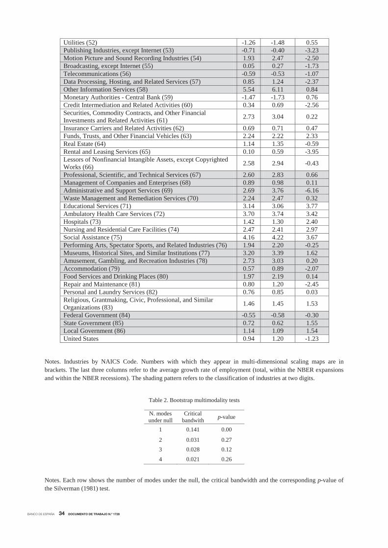
Computed from 1, 000 replications, Table 2 displays the critical window widths and the
p-values of the null hypothesis that the underlying density has at most m modes against the
alternative that it has more than m modes, with m = 1, 2, 3, 4. The tests should be applied
successively for an increasing number of modes until, for a certain number, the null is accepted.
Clearly, unimodality is rejected for all significance levels (p-value of 0.00), which suggests distinct
business cycle distribution dynamics for different population subgroups of industries. In addition,
the p-value corresponding to the null of bimodality versus trimodality is 0.27, which indicates
that the global distribution of ergodic business cycle distances is bimodal. It exhibits one hump
in the very low end representing the industries with a high level of business cycle synchronization
and then a larger hump representing those with idiosyncratic cycles.
Notably, the distribution shows a sizable concentration of mass in the middle range. This
could explain why the p-value for the test of three modes versus more than three modes falls
to 0.12, which is less conclusive. Using a significance level of 0.05, which is the most common
cut-off for p-values, the distribution is bimodal. However, using more conservative significance
levels, such as 0.15, the distribution would be trimodal (the p-value of four modes rises to 0.26).
Therefore, there are signals that the two modes located at the tails of the distribution could not
be well separated since the test does not exclude the possibility that the high-end range of the
distribution could be split into two subgroups.
Although useful, the kernel density estimation approach does not allow us to understand the
business cycle affiliations detected across the set of industries. To address this deficiency, we
employ clustering techniques and classical multi-dimensional scaling (see Timm, 2002, among
others) to the pairwise business cycle distances. Collecting the distances, πab0 , in the symmetric
matrix D, the goal of cluster analysis is to develop a classification scheme of our set of industries
in several distinct groups, since they present homogeneous business cycles. For this purpose,
we make use of dendograms, which are tree-structured graphs used to visualize the result of a
hierarchical clustering calculation. The end-points of the dendrogram depicted in Figure 6, whose
numbers appear in Table 1, represent the original industries. Clusters are successively combined,
forming the tree’s branches until the top of the graph. Although it is not easy to interpret,
the height of the tree represents the level of dissimilarity at which observations or clusters
are merged. Big jumps to join groups occur when there are high intergroup dissimilarities.
Therefore, a reasonable number of final groups is often obtained by cutting the dendogram at

BANCO DE ESPAÑA 19 DOCUMENTO DE TRABAJO N.º 1728
those junctures. In line with the results obtained with the kernel approach, the dendogram
shows that two (cutting at around 2) or three (cutting at around 1.5) clusters could be enough
to explain the business cycle affiliations across industries.
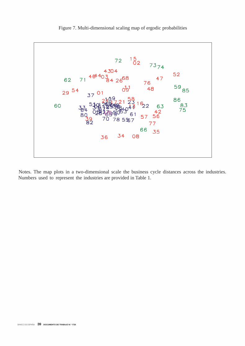
The multi-dimensional scaling map (see Appendix B) of business cycle similarities is reported
in Figure 7, whose plotted numbers refer to the industries listed in Table 1.6 Notably, the
industries grouped in the two/three different clusters of the dendogram belong to two/three
concentric circles, whose radius lengths reflect the business cycle dissimilarities from the centre
to the periphery. The U.S. economy appears in the centre or mass of the distribution of cyclical
similarities. The industries that experience the highest degree of synchronization with each other
and with the national cycle are displayed in the centre. Although these industries account for
a relatively small number, they represent 46.5% of total U.S. employment. Examples of large
industries that belong to this core are food services and drinking places, accommodation and
administrative and support services. However, the map also shows an intermediary zone and
a peripheral zone, indicating that other industries appear away from the attractor and do not
seem to be as closely related to the nation in terms of business cycle as the industries at the
core. The intermediary and peripherial zones are composed of industries representing 20.6% and
32.9% of total employment, respectively.
Let us have a deeper look at these business cycle affiliations. The core, in which the to-
tal U.S. employment is also included to facilitate comparison, is plotted in the centre of the
map and includes goods-producing industries, which typically experience the largest declines in
unemployment during recessions (Bureau of Labor Statistics, 2012), such as construction and
textiles, wood, furniture, and electronic products manufacturers. According to Goodman and
Mance (2011), complementary businesses that may suffer from ripple effects, such as furniture
and food stores, accommodations, appraisal services, motor vehicles, parts manufacturing, and
rental and leasing services, are also included. Finally, this core is also formed by other procycli-
cal industries (Bureau of Labor Statistics, 2012), such as wholesale and retail trade and personal
services, support activities and business services, especially administrative and waste services.7
The contrast between the national business cycle attractor and those industries plotted in
the intermediary zone of the perceptual map is a telling indication of their lower (albeit some)
business cycle concordance. In this middle circle, we observe some manufacturing industries
that may be subject to labour hoarding. Although they depend on the national business cycle,
6 In these maps, the axes are meaningless and the orientation of the picture is arbitrary.7Conlon (2011) documented that the payrolls of administrative and waste services shrank by more than 1
million positions during the Great Recession.
15

BANCO DE ESPAÑA 20 DOCUMENTO DE TRABAJO N.º 1728
8Parsons (1986) also documented a stronger tendency to hoard nonproduction labour.9Goodman (2001) finds that private education and health care services are countercyclical. In fact, employment
in these industries has decreased in only 1 of the 12 NBER recessions that have occurred since 1945 (Bureau of
Labor Statistics, 2012).10Groshen and Potter (2003) find that oil and gas extraction firms are countercyclical.11Christiano and Fitzgerald (1998) find that the business cycle components of the finance, insurance and real
estate industries exhibit low contemporaneous co-movement with aggregate employment. Goodman and Mance
(2011) show that employment in financial activities peaked one year before the official start of the Great Recession.
their synchronization could be diminished. According to Clark (1973), examples are durable
goods industries, such as chemical, rubber, plastic, primary metal and machinery manufactur-
ing, electrical equipment and building materials. In addition, Rotemberg and Summers (1990)
find that industries with a large ratio of nonproduction workers to employment also tend to
hoard labour.8 Examples are those businesses engaged in providing services in producing and
distributing information and cultural products and leisure activities. In addition, this cluster is
also formed by most of the industries providing transportation and related facilities, and ware-
housing and storage for goods. Interestingly, Christiano and Fitzgerald (1998) find that most of
the industries belonging to this cluster exhibit strong channels for intermediate goods.
The last cycle cluster is formed by some peripheral industries, which are less closely associ-
ated to the U.S. cycle. These industries are plotted further away from the business cycle centre,
which reflects their low sensitivity to the national cycle. In addition, they appear separate from
each other, which indicates that their business cycle shocks are idiosyncratic. This cluster is
mainly formed by those industries classified by Berman and Pfleeger (1997) as “not coinciden-
tally cyclical” industries. For some of these industries, the consequences of a negative demand
shock are relatively reduced since their product cannot normally be postponed. Examples are
businesses engaged in providing education and training, health care and social assistance, and
industries providing utility services, such as electric power, natural gas, steam supply, water
supply and sewage removal.9
In addition, this cluster includes sectors that depend highly on international shocks, such as
mineral extraction and its related supporting activities and gasoline stations, or on international
competition, such as wholesale electronic markets.10 Also belonging to this cluster are industries
providing financial services, not because they are not cyclical, but because they typically lead
the national cycle.11 Finally, we find in this cluster monetary authorities, and federal, state and
local government services. These industries provide necessities or public goods and demand for
these goods remains relatively strong throughout lows in the economy.
BANCO DE ESPAÑA 21 DOCUMENTO DE TRABAJO N.º 1728
BANCO DE ESPAÑA 22 DOCUMENTO DE TRABAJO N.º 1728
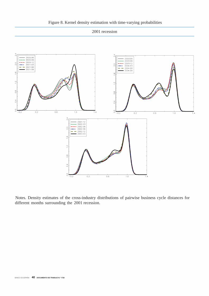
13Although it is not shown to save space, when bimodality is rejected, trimodality could not be rejected.
as it did in the peak. Finally, the middle mode appeared again when an increasing number of
industries initiated the recovery phase after the core.
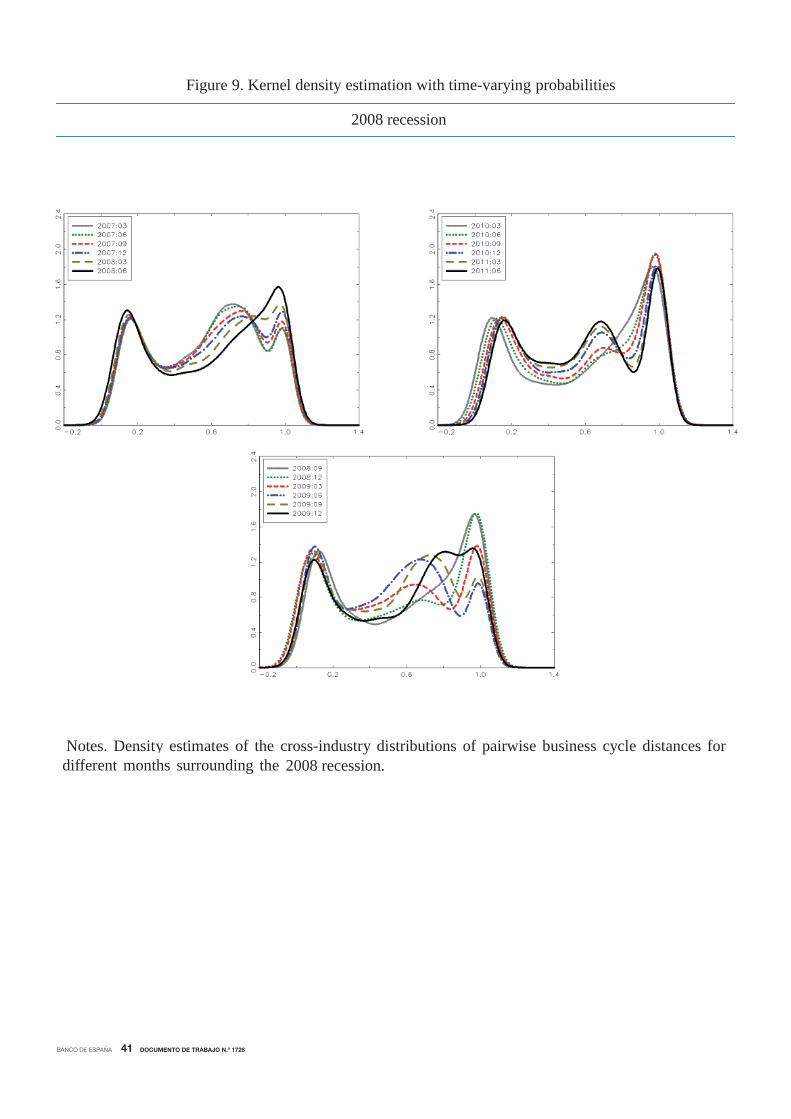
A similar but more accentuated pattern occurred during the 2008 recession. Figure 9 shows
that before the recession, the distribution seemed to be characterized by three modes. When the
peak occurred, the distribution became bimodal, since industries fell into recession sequentially,
providing evidence of a cascade effect. Once the economy was in recession, the trimodal pattern
in the distribution was recovered until the peak, when only the industries in the core initiated
the recovery and the distribution became bimodal again. The cycle ended when the economy
returned to the stable expansionary phase, and the distribution presented three modes, which
remained until the next turning point.
Noticeably, the distributions of pairwise business cycle distances in the 2008 recession show
a less pronounced mode in the right-end tail and a more pronounced mode in the left-end tail
than in the case of the 2001 recession. This indicates the presence of a larger mass of highly
synchronized industries and a smaller proportion of industries with idiosyncratic cycles, which
agrees with the evidence suggested in Figures 3 and 4 that the Great Recession recession was
more economy-wide than the 2001 recession.
In sum, we find that the propagation of micro-level shocks to national shocks is enhanced
when the mass shifts that characterize the turning points occur. A formal statistical test of this
pattern is provided by applying the modality tests in the density distributions of business cycle
similarities from January 1991 to May 2013. According to the plots of the kernel densities, the
nulls of unimodality (not shown here to save space) were clearly rejected for all months, since the
p-values were always quite close to zero. Figure 10 plots the p-values of the null of two versus
more than two modes. To facilitate the analysis, the figure includes shaded areas that refer
to the NBER-referenced recessions and a dashed line that refers to the 0.05 significance level.
The figure shows that bimodality is rejected during national expansions and recessions while it
cannot be rejected at any reasonable level of significance at the turning points.13 Notably, the
lagged business cycle behaviour that characterizes employment implies that bimodality appears
with some lags with respect to the NBER turning points. Therefore, the time-varying p-values
reaching the 0.05 threshold, which confirm the mass shifts in the distribution of the distances
on the pairwise industry cycles documented above, can be viewed as a mechanism that provides
assessments of when turning points in national (employment) business cycles take place.
Which industries are involved in these large changes in the distribution? To address this
question, Figure 11 captures the polarization tendencies around turning points documented in

BANCO DE ESPAÑA 23 DOCUMENTO DE TRABAJO N.º 1728
the density estimate analysis. For this purpose, the figure shows three representative months out
of the 269 multi-dimensional scaling maps computed in our sample period. Following the NBER
classification, the maps capture the across-industry business cycle distances in an expansion,
June 2000, and in a recession, March 2009. In both cases, the maps refer to months for which the
modality test detected trimodal distributions. The figure also shows the map dated September
2002, which is a month in which the modality test detected only two modes.
The within-expansion and within-recession maps look similar to the map computed from
the ergodic probabilities. According to their corresponding trimodal distributions of business
cycle distances, they show concentric circles of industries that exhibit highly, moderately and
lowly synchronized cycles with each other and with the national business cycle. However, the
map that refers to the period of transition from an expansion to a recession reflects a higher
dispersion across industries, which agrees with a distribution of business cycle distances that is
bimodal. According to this figure, it appears that the polarization could be owing to the fact
that some industries in the core were engaged in an expansionary phase, while others in the core
and the middle circle continued in a contractionary phase.
According to our results, the propagation of business cycle shocks across industries have fol-
lowed a regular pattern. The movements that occurred during the transitions around the peaks
are initiated by industries that are in the core and some industries that are in the middle mass.
Goods-producing industries, complementary businesses, wholesale and retail industries, support
activities and business services, especially administrative and waste services are amongst the
first to suffer from the negative effects of the recessions. Noticeable large and early declines
appear in construction and textiles, wood, furniture, and electronic products manufacturers,
especially in the 2008 recession.14 In line with Goodman and Mance (2011), we find that com-
plementary businesses that may suffer from ripple effects, such as furniture, accommodations,
appraisal services, motor vehicles, parts manufacturing, and rental and leasing services, also lose
employment in the early stages of the recessions.
14 In the 2008 recession, construction and manufacturing experienced their largest percentage declines in em-
ployment of the post-WWII era.
However, some industries that belong to the middle mass do not experience these severe job
cuts at the national peaks. Among these industries, we find durable goods industries, private
services industries, professional and technical services, recreational services, and industries pro-
viding transportation, warehousing and storage for goods. This reduced the synchronization
and the distribution of pairwise business cycle distances become bimodal as the middle mass is
pushed to the right-hand side that referred to industries with relatively reduced synchronization

BANCO DE ESPAÑA 24 DOCUMENTO DE TRABAJO N.º 1728
with the national recessions. Among these industries, we find businesses engaged in providing
education and training, health care and social assistance, industries providing utility services,
and industries providing necessities or public goods.
We postulate that the delay with which these industries faced the job losses could be caused
by at least one of the following determinants. First, since investments in durable goods usually
tend to follow manufacturing programs, the durable goods industry could have faced the nega-
tive effects of the recession with a delay as compared with that of the rapid-response industries.
Second, labor hoarding enables some of these industries, such as those involved in professional
and technical services, to hold on to workers with important firm-specific skills, who sometimes
require high training costs, and avoid the inevitable transaction costs related to laying-off per-
sonnel and hiring new workers at a later date. Third, some of the output of the consumption
goods sector is also used as intermediate goods in the production of durable goods, such as
machinery and equipment, which are in the middle mass and are exposed to ripple effects with
some lags.
In the course of the downturns, the industries of durable goods and intermediate goods,
which seemed to withstand the negative effects of the early stages of the national recession,
finally fall. With those industries loosing employment too, it seems that the recessions phase
cannot be avoided. In addition, despite the fact that labour hoarding means that firms do
not lay-off personnel with specific skills at the early stages of a national recession, it reduces
companies’ profitability during difficult times, in such a way that when the recession arrives, the
employment losses finally reach to these industries as well. Then, the recovered synchronicity
leads the distribution of business cycle distances to reshape to trimodal until the next trough
arrives.
In a similar fashion to the case of peaks, the recoveries in employment that characterize the
troughs are initiated by the same industries that first experienced a decline in employment in
the core and in the middle mass. Again, the uncertainty associated to recessions discourages
households and businesses from making purchases of durable goods until conditions improve. In
addition, the recoveries in employment of workers with high education, skill levels, or experience
is typically time consuming. This reduces the synchronization with the industries that showed
the recoveries in employment earlier, causing the middle-mass to shift to the right. The distri-
bution becomes bimodal until the industries exhibiting the delays in the recoveries start to hire
employees. At this stage, trimodality is restored again and the business cycle is completed.

BANCO DE ESPAÑA 25 DOCUMENTO DE TRABAJO N.º 1728
4 Concluding remarks
This paper is part of a growing empirical literature that analyzes the sources of interindustry
co-movements. It differs from this literature in several respects. First, the approach is in the
mould of “measurement without theory”. Using employment data, we ask whether industry-
level business cycles are coherent not only with the national business cycle, but also with each
other. Second, the filter used to compute the business cycle inferences is an extension of the
Markov-switching filter that allows for time-varying business cycle interdependence. Third,
nonparametric density estimation techniques are applied to assess the degree of population het-
erogeneity and to examine the changes in the business cycle distribution. Finally, heuristic
techniques of classical multi-dimensional scaling and clustering are used to understand the in-
dustry movements going in and out of recessions, which helps us to identify changes in cyclical
affiliations.
Our main results are the following. First, there is a large heterogeneity in the distribution
of business cycle similarities, implying the existence of population groups that follow distinct
distributional dynamics. Second, there is not a monotone movement toward the emergence of
an increasingly cohesive national business cycle core. The positions of the lower mode, which
comprises extremely synchronized industries, and the cluster at the high end of the distribution,
which represents industries with idiosyncratic cycles, are relatively stable over time. However,
the position of a third, middle mode when the economy is in expansionary or recessionary phases
jumps up substantially during the period of transition from one phase to another, switching
from pairwise business cycle distances of just over 0.5 to almost one. Therefore, the proposed
framework is able to provide assessments of when a national turning point takes place and how
the business cycle shocks propagate across industries.
The model used in this paper provides a solid foundation for starting a line of research that
seeks to explain the determinants of the business cycle affiliations across industries. Various
factors have been put forward in the literature that may affect business cycle synchronization,
ranging from the proportion of fixed and variable costs, industry concentration, product differ-
entiation and dependence on external finance. However, the modifications of the model used in
the paper to capture the changes in affiliations would be substantial; therefore, this task is left
to future research.

BANCO DE ESPAÑA 26 DOCUMENTO DE TRABAJO N.º 1728
Appendix AThis appendix describes the estimation of the parameters in vector θ and the inference on
s∗ab,T , which is performed through a multi-move Gibbs-sampling procedure. The distribution
of the parameters can be approximated by the empirical distributions of simulated values, by
iterating the following steps.
STEP 1. The Gibbs sampler is started with arbitrary starting values for the parameters of
the model, θ0, which are used to generate s∗1ab,T |yab,T , θ0. For this purpose, we run the Markov-switching filter described in Section 2 and obtain the filtered probabilities p(s∗ab,t|yab,t, θ0). Todraw the state variables, we employ the following result:
p s∗ab,T |yab,T , θ0 = p s∗ab,T |yab,T , θ0T−1
t=1
p(s∗ab,t|s∗ab,t+1, yab,t, θ0). (A1)
The last iteration of the Markov-switching filter provides us with p s∗ab,T |yab,T , θ0 , from which
s∗ab,T is generated. To generate s∗ab,t, with t = 1, ..., T − 1, we use
p(s∗ab,t|s∗ab,t+1, yab,t, θ0) = p(s∗ab,t+1|s∗ab,t) ∝ p(s∗ab,t|yab,t, θ0), (A2)
where p(s∗ab,t|s∗ab,t+1) refers to the transition probabilities, which are included in θ0. Using this
expression, it is straightforward to generate s∗ab,t by computing the probability of state i from
p(s∗ab,t = i|s∗ab,t+1, yab,t, θ0) =p(s∗ab,t+1|s∗ab,t = i)p(s∗ab,t = i|yab,t, θ0)
j=i
p(s∗ab,t+1|s∗ab,t = j)p(s∗ab,t = j|yab,t, θ0). (A3)
Using random numbers from a uniform distribution between 0 and 1, s∗1ab,t is set to a par-
ticular state i by comparing the probability of this state with the random numbers. Follow-
ing a similar reasoning, one can also generate s1k,T = s1k,1, ..., s1k,T , v
1ab,T = v1ab,1, ..., v
1ab,T and
ς1ab,T = ς1ab,1, ..., ς1ab,T , for any industry k and any pair a and b at any time t = 1, ..., T .
STEP 2. The generated state variables are used to draw the transition probabilities pkij , pabij
and qabij . Since these parameters are drawn in a similar way, we focus only on pkij to save space.
Conditional on sk,T , the transition probabilities are independent of the data set yab,T and the
model’s other parameters. Given s1k,T , let nkij , i, j = 0, 1 be the total number of transitions from
state i to state j in industry k. By taking the beta family of distributions as conjugate priors,
pkii˜beta(ukii, u
kij), (A4)
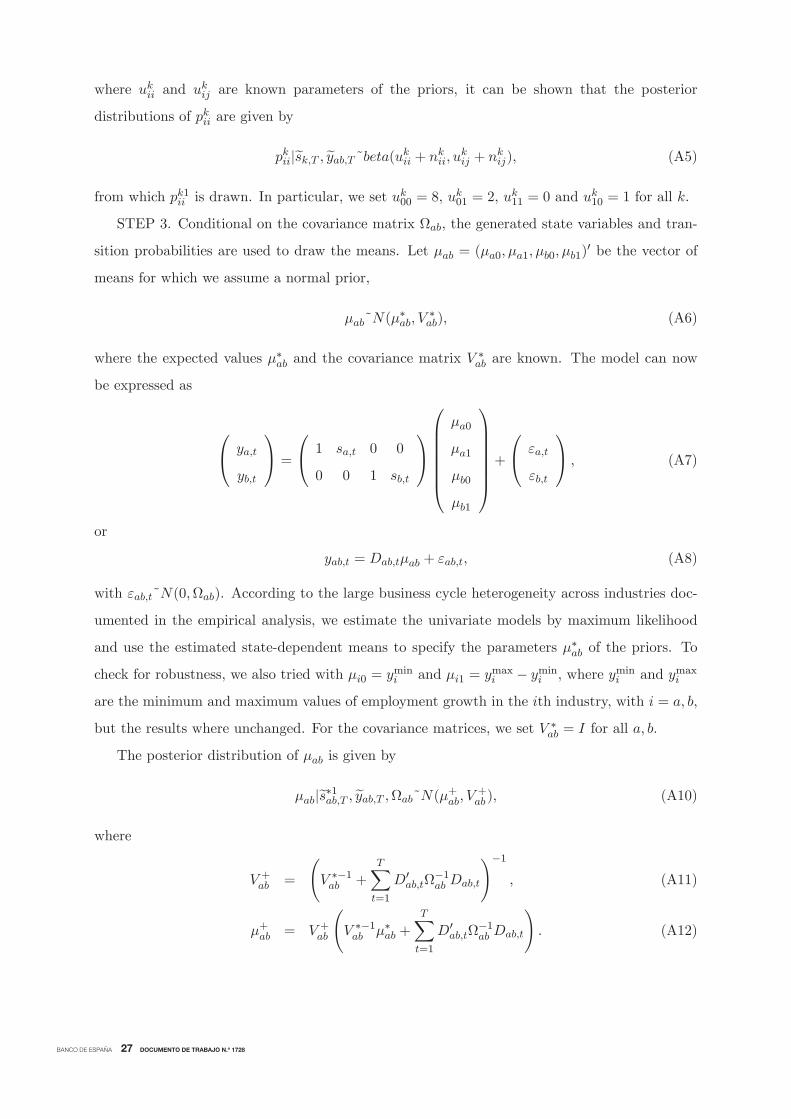
BANCO DE ESPAÑA 27 DOCUMENTO DE TRABAJO N.º 1728
where ukii and ukij are known parameters of the priors, it can be shown that the posterior
distributions of pkii are given by
pkii|sk,T , yab,T ˜beta(ukii + nkii, ukij + nkij), (A5)
from which pk1ii is drawn. In particular, we set uk00 = 8, u
k01 = 2, u
k11 = 0 and u
k10 = 1 for all k.
STEP 3. Conditional on the covariance matrix Ωab, the generated state variables and tran-
sition probabilities are used to draw the means. Let μab = (μa0,μa1,μb0,μb1) be the vector of
means for which we assume a normal prior,
μab˜N(μ∗ab, V
∗ab), (A6)
where the expected values μ∗ab and the covariance matrix V∗ab are known. The model can now
be expressed as
⎛⎝ ya,t
yb,t
⎞⎠ =
⎛⎝ 1
0
sa,t
0
0
1
0
sb,t
⎞⎠⎛⎜⎜⎜⎜⎜⎜⎝
μa0
μa1
μb0
μb1
⎞⎟⎟⎟⎟⎟⎟⎠+⎛⎝ εa,t
εb,t
⎞⎠ , (A7)
or
yab,t = Dab,tμab + εab,t, (A8)
with εab,t˜N(0,Ωab). According to the large business cycle heterogeneity across industries doc-
umented in the empirical analysis, we estimate the univariate models by maximum likelihood
and use the estimated state-dependent means to specify the parameters μ∗ab of the priors. To
check for robustness, we also tried with μi0 = ymini and μi1 = y
maxi − ymini , where ymini and ymaxi
are the minimum and maximum values of employment growth in the ith industry, with i = a, b,
but the results where unchanged. For the covariance matrices, we set V ∗ab = I for all a, b.
The posterior distribution of μab is given by
μab|s∗1ab,T , yab,T ,Ωab˜N(μ+ab, V +ab ), (A10)
where
V +ab = V ∗−1ab +
T
t=1
Dab,tΩ−1ab Dab,t
−1, (A11)
μ+ab = V +ab V ∗−1ab μ∗ab +T
t=1
Dab,tΩ−1ab Dab,t . (A12)

BANCO DE ESPAÑA 28 DOCUMENTO DE TRABAJO N.º 1728
STEP 4. Conditional on the generated state variables, transition probabilities and state-
dependent means, the parameters of the covariance matrix are drawn. For this purpose, we use
the Wishart distribution as the conjugate prior of the inverse covariance matrix,
Ω−1ab ∼W (Σ∗−1ab , r∗ab), (A13)
where Σ∗ab and r∗ab are known. In particular, we set Σ
∗ab = I and r
∗ab = 0. Then, the posterior
distribution is
Ω−1ab |s∗1ab,T , yab,T ,μ1ab ∼W (Σ+−1ab , r+ab), (A14)
where
r+ab = T + r∗ab, (A15)
Σ+−1ab = Σ∗−1ab +
T
t=1
yab,t −D1ab,tμ1ab yab,t −D1ab,tμ1ab . (A16)
Steps 1 through 4 can be iterated L+M times, where L is large enough to ensure that the
Gibbs sampler has converged. Thus, the marginal distributions of the state variables and the
parameters of the model can be approximated by the empirical distribution of the M simulated
values.

BANCO DE ESPAÑA 29 DOCUMENTO DE TRABAJO N.º 1728
BANCO DE ESPAÑA 30 DOCUMENTO DE TRABAJO N.º 1728
References
[1] Acemoglu, D., V. Carvalho, A. Ozdaglar, and A. Tahbaz-Salehi (2012), The network origins
of aggregate fluctuations. Econometrica 80: 1977-2016.
[2] Barker, M. (2011), Manufacturing employment hard hit during the 2007-09 recession.
Monthly Labor Review, April: 28-33.
[3] Bengoechea, P., M. Camacho, and G. Perez Quiros (2006), A useful tool for forecasting the
Euro-area business cycle phases. International Journal of Forecasting 22: 735-749.
[4] Berman, J. and J. Pfleeger (1997), Which industries are sensitive to business cycles?
Monthly Labor Review, February: 19-25.
[5] Bureau of Labor Statistics (2012), The recession of 2007-2009. BLS Spotlight on Statistics,
February.
[6] Camacho, M., and G. Perez Quiros (2006), A new framework to analyze business cycle
synchronization. In: Milas, C., Rothman, P., and van Dijk, D. Nonlinear Time Series
Analysis of Business Cycles. Elsevier’s Contributions to Economic Analysis series. Chapter
5 (pp. 133-149). Elsevier, Amsterdam.
[7] Carlino, G., R. H. DeFina (2004), How strong is co-movement in employment over the
business cycle? Evidence from state/industry data. Journal of Urban Economics 55: 298-
315.
[8] Carvalho, V.M., (2008), Aggregate Fluctuations and the Network Structure of Intersectoral
Trade. Working Paper, CREI.
[9] Christiano, L., and T. Fitzgerald (1998), The business cycle: it’s still a puzzle. Economic
Perspectives, Fourth Quarter: 56-83.
[10] Clark, S. (1973), Labor hoarding in durable goods industries. American Economic Review
63: 811-824.
[11] Conlon. F. (2011), Professional and business services: employment trends in the 2007-09
recession. Monthly Labor Review April: 34-39.
[12] Dupor, B., 1999, Aggregation and Irrelevance in Multi-Sector Models. Journal of Monetary
Economics 43: 391—409.
BANCO DE ESPAÑA 31 DOCUMENTO DE TRABAJO N.º 1728
[13] Filardo, A. (1997), Cyclical implications of the declining manufacturing employment share.
Federal Reserve Bank of Kansas City Economic Review II: 63-87.
[14] Foerster, A., P. Sarte, and M. Watson (2011), Sectorial versus aggregate shocks: a structural
factor analysis of industrial production. Journal of Political Economy 119: 1-38.
[15] Forni, M., and Reichlin, L. (1998), Let’s Get Real: A Factor Analytical Approach to Dis-
aggregated Business Cycle Dynamics. Review of Economic Studies 65: 453-473.
[16] Gabaix, X. (2011), The granular origins of aggregate fluctuations. Econometrica 79: 733-
772.
[17] Goodman, W. (2001), Employment in services industries affected by recessions and expan-
sions. Monthly Labor Review October: 3-11.
[18] Goodman, W., and S. Mance (2011), Employment loss and the 2007-09 recession: an
overview. Monthly Labor Review April: 3-12.
[19] Groshen, E., and S. Potter (2003), Has structural change contributed to a jobless recovery?
Current Issues in Economics and Finance 9 (August).
[20] Hamilton, J. (1989), A new approach to the economic analysis of nonstationary time series
and the business cycles. Econometrica 57: 357-384.
[21] Hamilton, J., and M. Owyang (2012), The Propagation of Regional Recessions. The Review
of Economics and Statistics, 94: 935-947.
[22] Horvath, M. (1998), Cyclicality and Sectoral Linkages: Aggregate Fluctuations From Sec-
toral Shocks. Review of Economic Dynamics 1: 781-808.
[23] Horvath, M. (2000), Sectoral Shocks and Aggregate Fluctuations. Journal of Monetary
Economics 45: 69—106.
[24] Karadimitropoulou, A., and Leon-Ledesma, M. (2013), World, Country, and Sector Factors
in International Business Cycles. Journal of Economic Dynamics and Control, 2913-2927.
[25] Leiva-Leon, D. (2016), Measuring Business Cycles Intra-Synchronization in US: A Regime-
Switching Interdependence Framework. Oxford Bulletin of Economics and Statistics, Forth-
coming.
[26] Long, J.B., and Plosser, C.I. (1983), Real Business Cycles. Journal of Political Economy
91: 39-69.

BANCO DE ESPAÑA 32 DOCUMENTO DE TRABAJO N.º 1728
[27] Long, J.B., and Plosser, C.I. (1987), Sectoral vs. Aggregate Shocks in the Business Cycle.
American Economic Review 77, 333-336.
[28] Malmendier, U., and S. Nagel (2011), Depression babies: Do macroeconomic experiences
affect risk taking? The Quarterly Journal of Economics 126: 373-416.
[29] Owyang, M., J. Piger, and H. Wall (2005), Business cycle phases in the U.S. states. The
Review of Economics and Statistics 87: 604-616.
[30] Owyang, M., J. Piger, H. Wall, and C. Wheeler (2008), The economic performance of cities:
A Markov-switching approach. Journal of Urban Economics 64: 538-550.
[31] Parsons O. (1986), The employment relationship: Job attachment, work effort and the
nature of contracts. Handbook of Labor Economics. Ashenfelter O, Layard R (eds.), Elsevier:
New York.
[32] Peterson, B., and S. Strongin (1996), Why are some industries more cyclical than others?
Journal of Business and Economic Statistics 14(2) : 189-198.
[33] Phillips, K. (1991), A two-country model of stochastic output with changes in regime.
Journal of International Economics, 31: 121-142.
[34] Rotemberg J, and L. Summers (1990), Inflexible Prices and Procyclical productivity. Quar-
terly Journal of Economics 105: 851-874.
[35] Shea, J. (2002), Complementarities and Comovements. Journal of Money, Credit, and Bank-
ing 34: 412—433.
[36] Silverman, B. (1981), Using kernel density estimates to investigate multimodality. Journal
of the Royal Statistical Society, Series B 43: 97-99.
[37] Timm, N. (2002), Applied multivariate analysis. Springer texts in Statistics.
[38] Urquhart, M. (1981), The services industry: Is it recession-proof? Monthly Labor Review
October: 12-18.
BANCO DE ESPAÑA 33 DOCUMENTO DE TRABAJO N.º 1728
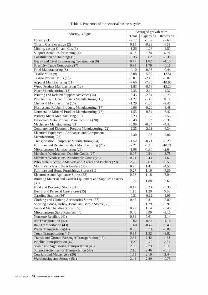
Table 1. Properties of the sectorial business cycles
Industry, 3 digits Averaged growth rates Total Expansion Recession
Forestry (1) -2.17 -1.52 -7.60 Oil and Gas Extraction (2) 0.15 -0.38 4.58 Mining, except Oil and Gas (3) -1.26 -1.23 -1.53 Support Activities for Mining (4) 4.03 3.74 6.39 Construction of Buildings (5) -0.35 0.62 -8.38 Heavy and Civil Engineering Construction (6) 0.47 1.02 -4.10 Specialty Trade Contractors (7) 0.93 1.79 -6.18 Food Manufacturing (8) -0.10 -0.05 -0.44 Textile Mills (9) -6.08 -5.30 -12.51 Textile Product Mills (10) -3.01 -2.40 -8.02 Apparel Manufacturing (11) -7.66 -7.26 -10.96 Wood Product Manufacturing (12) -1.83 -0.58 -12.20 Paper Manufacturing (13) -2.35 -2.10 -4.37 Printing and Related Support Activities (14) -2.45 -2.04 -5.79 Petroleum and Coal Products Manufacturing (15) -1.27 -1.49 0.51 Chemical Manufacturing (16) -1.20 -1.05 -2.48 Plastics and Rubber Products Manufacturing (17) -0.96 -0.29 -6.48 Nonmetallic Mineral Product Manufacturing (18) -1.55 -0.84 -7.42 Primary Metal Manufacturing (19) -2.23 -1.59 -7.56 Fabricated Metal Product Manufacturing (20) -0.43 0.17 -5.35 Machinery Manufacturing (21) -0.96 -0.54 -4.42 Computer and Electronic Product Manufacturing (22) -2.35 -2.11 -4.34 Electrical Equipment, Appliance, and Component Manufacturing (23) -2.30 -1.96 -5.06
Transportation Equipment Manufacturing (24) -1.52 -0.71 -8.20 Furniture and Related Product Manufacturing (25) -2.21 -1.18 -10.71 Miscellaneous Manufacturing (26) -1.98 -1.90 -2.64 Merchant Wholesalers, Durable Goods (27) 0.07 0.54 -3.78 Merchant Wholesalers, Nondurable Goods (28) 0.21 0.43 -1.61 Wholesale Electronic Markets and Agents and Brokers (29) 2.28 2.63 -0.55 Motor Vehicle and Parts Dealers (30) 0.76 1.41 -4.58 Furniture and Home Furnishings Stores (31) 0.27 1.19 -7.39 Electronics and Appliance Stores (32) 0.63 1.18 -3.94 Building Material and Garden Equipment and Supplies Dealers (33) 1.29 1.88 -3.61
Food and Beverage Stores (34) 0.17 0.23 -0.36 Health and Personal Care Stores (35) 1.13 1.20 0.56 Gasoline Stations (36) -0.31 -0.12 -1.95 Clothing and Clothing Accessories Stores (37) 0.42 0.81 -2.80 Sporting Goods, Hobby, Book, and Music Stores (38) 1.05 1.29 -0.91 General Merchandise Stores (39) 0.97 1.14 -0.40 Miscellaneous Store Retailers (40) 0.46 0.90 -3.16 Nonstore Retailers (41) 0.31 0.61 -2.14 Air Transportation (42) -0.62 -0.55 -1.16 Rail Transportation (43) -0.68 -0.47 -2.43 Water Transportation(44) 0.55 0.73 -0.89 Truck Transportation (45) 0.94 1.52 -3.82 Transit and Ground Passenger Transportation (46) 2.34 2.42 1.68 Pipeline Transportation (47) -1.27 -1.70 2.31 Scenic and Sightseeing Transportation (48) 2.59 2.79 1.00 Support Activities for Transportation (49) 2.18 2.46 -0.12 Couriers and Messengers (50) 1.69 2.19 -2.44 Warehousing and Storage (51) 2.41 2.80 -0.75
BANCO DE ESPAÑA 34 DOCUMENTO DE TRABAJO N.º 1728
Utilities (52) -1.26 -1.48 0.55 Publishing Industries, except Internet (53) -0.71 -0.40 -3.23 Motion Picture and Sound Recording Industries (54) 1.93 2.47 -2.50 Broadcasting, except Internet (55) 0.05 0.27 -1.73 Telecommunications (56) -0.59 -0.53 -1.07 Data Processing, Hosting, and Related Services (57) 0.85 1.24 -2.37 Other Information Services (58) 5.54 6.11 0.84 Monetary Authorities - Central Bank (59) -1.47 -1.73 0.76 Credit Intermediation and Related Activities (60) 0.34 0.69 -2.56 Securities, Commodity Contracts, and Other Financial Investments and Related Activities (61) 2.73 3.04 0.22
Insurance Carriers and Related Activities (62) 0.69 0.71 0.47 Funds, Trusts, and Other Financial Vehicles (63) 2.24 2.22 2.33 Real Estate (64) 1.14 1.35 -0.59 Rental and Leasing Services (65) 0.10 0.59 -3.95 Lessors of Nonfinancial Intangible Assets, except Copyrighted Works (66) 2.58 2.94 -0.43
Professional, Scientific, and Technical Services (67) 2.60 2.83 0.66 Management of Companies and Enterprises (68) 0.89 0.98 0.11 Administrative and Support Services (69) 2.69 3.76 -6.16 Waste Management and Remediation Services (70) 2.24 2.47 0.32 Educational Services (71) 3.14 3.06 3.77 Ambulatory Health Care Services (72) 3.70 3.74 3.42 Hospitals (73) 1.42 1.30 2.40 Nursing and Residential Care Facilities (74) 2.47 2.41 2.97 Social Assistance (75) 4.16 4.22 3.67 Performing Arts, Spectator Sports, and Related Industries (76) 1.94 2.20 -0.25 Museums, Historical Sites, and Similar Institutions (77) 3.20 3.39 1.62 Amusement, Gambling, and Recreation Industries (78) 2.73 3.03 0.20 Accommodation (79) 0.57 0.89 -2.07 Food Services and Drinking Places (80) 1.97 2.19 0.14 Repair and Maintenance (81) 0.80 1.20 -2.45 Personal and Laundry Services (82) 0.76 0.85 0.03 Religious, Grantmaking, Civic, Professional, and Similar Organizations (83) 1.46 1.45 1.53
Federal Government (84) -0.55 -0.58 -0.30 State Government (85) 0.72 0.62 1.55 Local Government (86) 1.14 1.09 1.54 United States 0.94 1.20 -1.23
Notes. Industries by NAICS Code. Numbers with which they appear in multi-dimensional scaling maps are in brackets. The last three columns refer to the average growth rate of employment (total, within the NBER expansions and within the NBER recessions). The shading pattern refers to the classification of industries at two digits.
Notes. Each row shows the number of modes under the null, the critical bandwidth and the corresponding p-value of the Silverman (1981) test.
Table 2. Bootstrap multimodality tests
N. modes under null
Critical bandwith p-value
1 0.141 0.00
2 0.031 0.27 3 0.028 0.12
4 0.021 0.26
BANCO DE ESPAÑA 35 DOCUMENTO DE TRABAJO N.º 1728
Figure 1. U.S. employment
-6
-4
-2
0
2
4
1991.01 1995.06 1999.11 2004.04 2008.09 2013.02
Notes. The figure plots annual growth rates. Shaded areas indicate NBER recessions.
.00
.04
.08
.12
.16
.20
-16 -14 -12 -10 -8 -6 -4 -2 0 2 4 6 8 10
Dens
ity
Recession
Expansion
Figure 2. Kernel distribution over the cycle
Notes. The figure plots the kernel distribution of year-over-year employment growth across industries. are obtained from the NBER business cycle dates. Expansions and recessions are obtained from the NBER business cycle dates.
BANCO DE ESPAÑA 36 DOCUMENTO DE TRABAJO N.º 1728
Figure 3. Univariate Markov-switching analysis
0.0 0.2 0.4 0.6 0.8 1.0
2001 recession
1999Q4 2000Q1 2000Q2 2000Q3 2000Q4
2001Q1 2001Q2 2001Q3 2001Q4 2002Q1
2002Q2 2002Q3 2002Q4 2003Q1 2003Q2
Notes. The figure plots the choropleth map of industries for different quarters surrounding the 2001 recession (bold red letters). Each chart correspondsto one quarter; the partitions of each chart represent U.S. industries; and the size of the partitions represents the industries’ share of nationalemployment. The darker an industry’s partition, the higher the probability of recession for that industry during that quarter. To see each chart in detailgo to https://sites.google.com/site/daniloleivaleon/us-industrial-cycles.
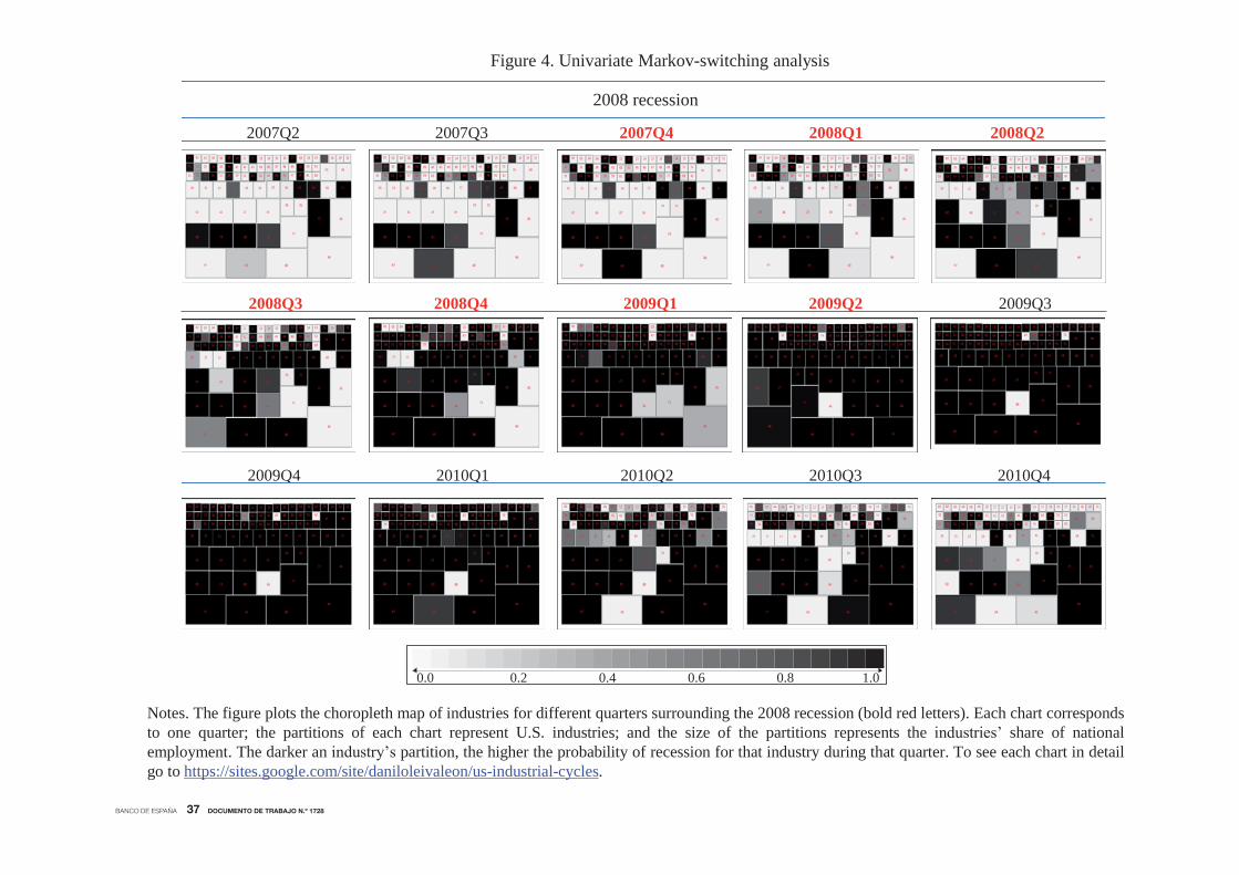
BANCO DE ESPAÑA 37 DOCUMENTO DE TRABAJO N.º 1728
0.0 0.2 0.4 0.6 0.8 1.0
2009Q4 2010Q1 2010Q2 2010Q3 2010Q4
2008Q3 2008Q4 2009Q1 2009Q2 2009Q3
2007Q2 2007Q3 2007Q4 2008Q1 2008Q2
g g y
2008 recession
Figure 4. Univariate Markov-switching analysis
Notes. The figure plots the choropleth map of industries for different quarters surrounding the 2008 recession (bold red letters). Each chart correspondsto one quarter; the partitions of each chart represent U.S. industries; and the size of the partitions represents the industries’ share of nationalemployment. The darker an industry’s partition, the higher the probability of recession for that industry during that quarter. To see each chart in detailgo to https://sites.google.com/site/daniloleivaleon/us-industrial-cycles.
BANCO DE ESPAÑA 38 DOCUMENTO DE TRABAJO N.º 1728
Figure 5. Kernel density estimation from ergodic probabilities
14 53 45 78 6 7 55 70 81 19 27 50 69 20 79 38 51 67 US82 22 23 41 32 61 40 49 5 28 10 64 65 12 18 33 25 30 37 31 80 1 17 26 9 13 11 16 24 3 43 21 68 2 4 15 47 52 8 35 77 29 54 34 36 39 84 44 76 46 42 56 57 58 48 59 85 73 75 86 60 62 63 66 71 83 72 740
0.5
1
1.5
2
Notes. Density estimates of the cross-industry distributions of pairwise business cycle distances using ergodic probabilities.
Figure 6. Cluster analysis with ergodic probabilities
are merged. Numbers used to represent the industries are provided in Table 1. Notes. The dendogram’s heights represent the level of dissimilarity at which observations or clusters
BANCO DE ESPAÑA 39 DOCUMENTO DE TRABAJO N.º 1728
Figure 7. Multi-dimensional scaling map of ergodic probabilities
Numbers used to represent the Notes. The map plots in a two-dimensional scale the business cycle distances across the industries.
industries are provided in Table 1.
BANCO DE ESPAÑA 40 DOCUMENTO DE TRABAJO N.º 1728
Figure 8. Kernel density estimation with time-varying probabilities
2001 recession
different months surrounding the Notes. Density estimates of the cross-industry distributions of pairwise business cycle distances for
2001 recession.
BANCO DE ESPAÑA 41 DOCUMENTO DE TRABAJO N.º 1728
Figure 9. Kernel density estimation with time-varying probabilities
2008 recession
Notes. Density estimates of the cross-industry distributions of pairwise business cycle distances for different months surrounding the 2008 recession.
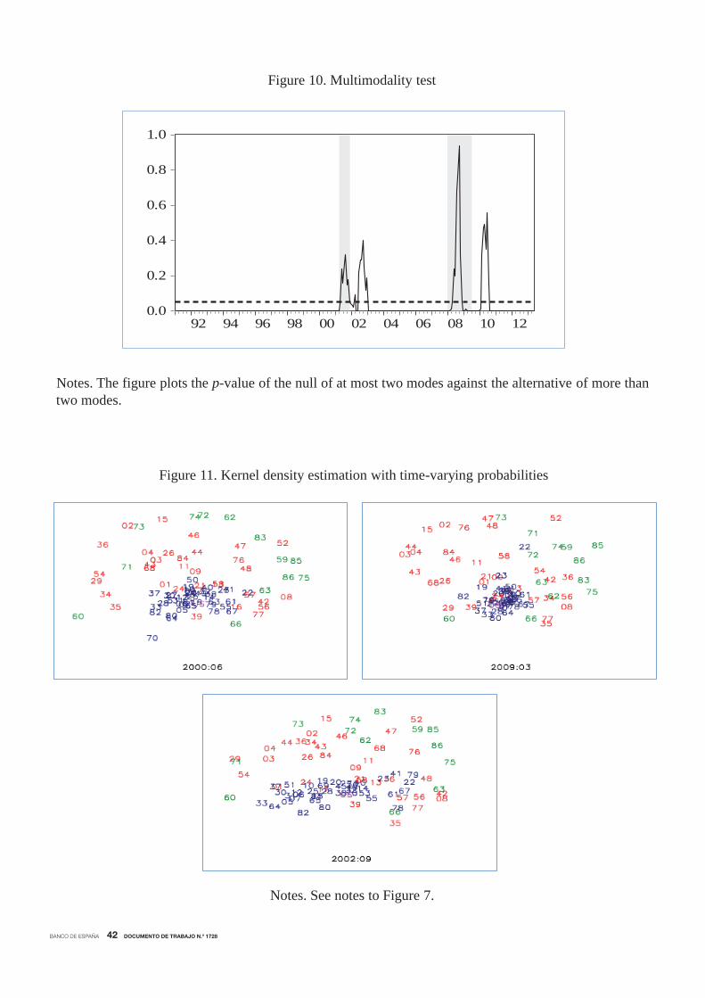
BANCO DE ESPAÑA 42 DOCUMENTO DE TRABAJO N.º 1728
0.0
0.2
0.4
0.6
0.8
1.0
92 94 96 98 00 02 04 06 08 10 12
Figure 10. Multimodality test
Notes. The figure plots the p-value of the null of at most two modes against the alternative of more than two modes.
Figure 11. Kernel density estimation with time-varying probabilities
Notes. See notes to Figure 7.
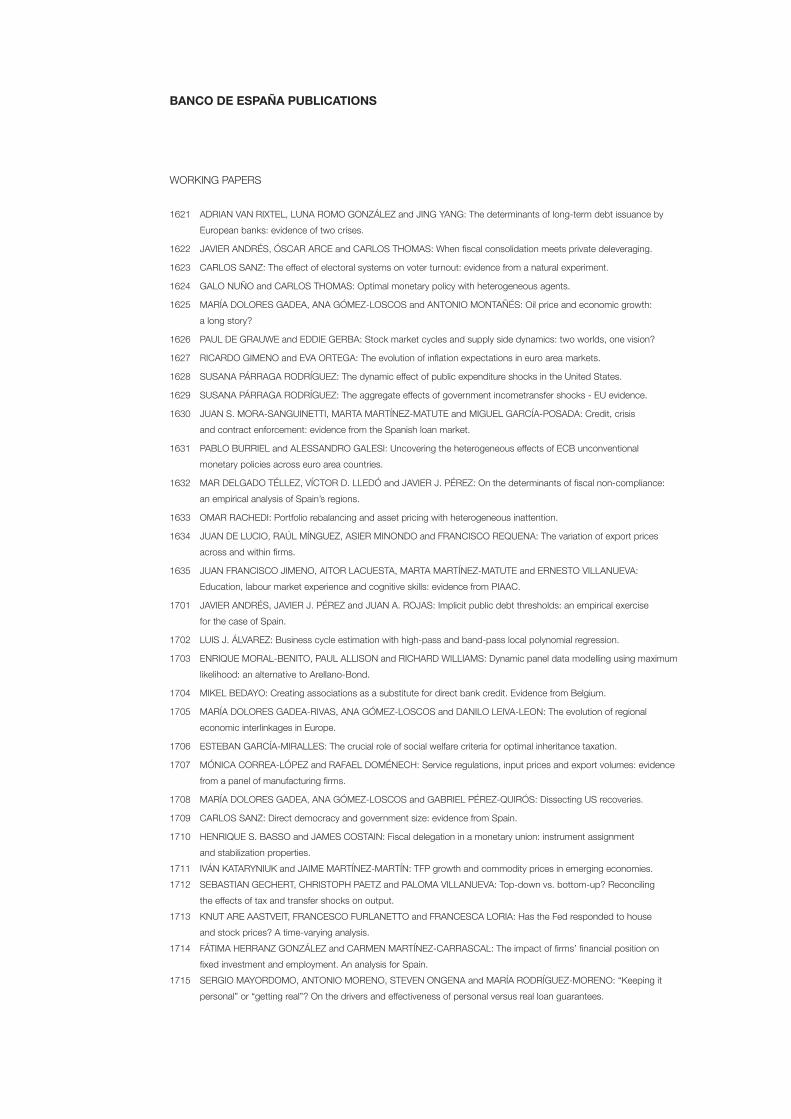
BANCO DE ESPAÑA PUBLICATIONS
WORKING PAPERS
1621 ADRIAN VAN RIXTEL, LUNA ROMO GONZÁLEZ and JING YANG: The determinants of long-term debt issuance by
European banks: evidence of two crises.
1622 JAVIER ANDRÉS, ÓSCAR ARCE and CARLOS THOMAS: When fi scal consolidation meets private deleveraging.
1623 CARLOS SANZ: The effect of electoral systems on voter turnout: evidence from a natural experiment.
1624 GALO NUÑO and CARLOS THOMAS: Optimal monetary policy with heterogeneous agents.
1625 MARÍA DOLORES GADEA, ANA GÓMEZ-LOSCOS and ANTONIO MONTAÑÉS: Oil price and economic growth:
a long story?
1626 PAUL DE GRAUWE and EDDIE GERBA: Stock market cycles and supply side dynamics: two worlds, one vision?
1627 RICARDO GIMENO and EVA ORTEGA: The evolution of infl ation expectations in euro area markets.
1628 SUSANA PÁRRAGA RODRÍGUEZ: The dynamic effect of public expenditure shocks in the United States.
1629 SUSANA PÁRRAGA RODRÍGUEZ: The aggregate effects of government incometransfer shocks - EU evidence.
1630 JUAN S. MORA-SANGUINETTI, MARTA MARTÍNEZ-MATUTE and MIGUEL GARCÍA-POSADA: Credit, crisis
and contract enforcement: evidence from the Spanish loan market.
1631 PABLO BURRIEL and ALESSANDRO GALESI: Uncovering the heterogeneous effects of ECB unconventional
monetary policies across euro area countries.
1632 MAR DELGADO TÉLLEZ, VÍCTOR D. LLEDÓ and JAVIER J. PÉREZ: On the determinants of fi scal non-compliance:
an empirical analysis of Spain’s regions.
1633 OMAR RACHEDI: Portfolio rebalancing and asset pricing with heterogeneous inattention.
1634 JUAN DE LUCIO, RAÚL MÍNGUEZ, ASIER MINONDO and FRANCISCO REQUENA: The variation of export prices
across and within fi rms.
1635 JUAN FRANCISCO JIMENO, AITOR LACUESTA, MARTA MARTÍNEZ-MATUTE and ERNESTO VILLANUEVA:
Education, labour market experience and cognitive skills: evidence from PIAAC.
1701 JAVIER ANDRÉS, JAVIER J. PÉREZ and JUAN A. ROJAS: Implicit public debt thresholds: an empirical exercise
for the case of Spain.
1702 LUIS J. ÁLVAREZ: Business cycle estimation with high-pass and band-pass local polynomial regression.
1703 ENRIQUE MORAL-BENITO, PAUL ALLISON and RICHARD WILLIAMS: Dynamic panel data modelling using maximum
likelihood: an alternative to Arellano-Bond.
1704 MIKEL BEDAYO: Creating associations as a substitute for direct bank credit. Evidence from Belgium.
1705 MARÍA DOLORES GADEA-RIVAS, ANA GÓMEZ-LOSCOS and DANILO LEIVA-LEON: The evolution of regional
economic interlinkages in Europe.
1706 ESTEBAN GARCÍA-MIRALLES: The crucial role of social welfare criteria for optimal inheritance taxation.
1707 MÓNICA CORREA-LÓPEZ and RAFAEL DOMÉNECH: Service regulations, input prices and export volumes: evidence
from a panel of manufacturing fi rms.
1708 MARÍA DOLORES GADEA, ANA GÓMEZ-LOSCOS and GABRIEL PÉREZ-QUIRÓS: Dissecting US recoveries.
1709 CARLOS SANZ: Direct democracy and government size: evidence from Spain.
1710 HENRIQUE S. BASSO and JAMES COSTAIN: Fiscal delegation in a monetary union: instrument assignment
and stabilization properties.
1711 IVÁN KATARYNIUK and JAIME MARTÍNEZ-MARTÍN: TFP growth and commodity prices in emerging economies.
1712 SEBASTIAN GECHERT, CHRISTOPH PAETZ and PALOMA VILLANUEVA: Top-down vs. bottom-up? Reconciling
the effects of tax and transfer shocks on output.
1713 KNUT ARE AASTVEIT, FRANCESCO FURLANETTO and FRANCESCA LORIA: Has the Fed responded to house
and stock prices? A time-varying analysis.
1714 FÁTIMA HERRANZ GONZÁLEZ and CARMEN MARTÍNEZ-CARRASCAL: The impact of fi rms’ fi nancial position on
fi xed investment and employment. An analysis for Spain.
1715 SERGIO MAYORDOMO, ANTONIO MORENO, STEVEN ONGENA and MARÍA RODRÍGUEZ-MORENO: “Keeping it
personal” or “getting real”? On the drivers and effectiveness of personal versus real loan guarantees.
1716 FRANCESCO FURLANETTO and ØRJAN ROBSTAD: Immigration and the macroeconomy: some new empirical evidence.
1717 ALBERTO FUERTES: Exchange rate regime and external adjustment: an empirical investigation for the U.S.
1718 CRISTINA GUILLAMÓN, ENRIQUE MORAL-BENITO and SERGIO PUENTE: High growth fi rms in employment and
productivity: dynamic interactions and the role of fi nancial constraints.
1719 PAULO SOARES ESTEVES and ELVIRA PRADES: On domestic demand and export performance in the euro area
countries: does export concentration matter?
1720 LUIS J. ÁLVAREZ and ANA GÓMEZ-LOSCOS: A menu on output gap estimation methods.
1721 PAULA GIL, FRANCISCO MARTÍ, JAVIER J. PÉREZ, ROBERTO RAMOS and RICHARD MORRIS: The output effects
of tax changes: narrative evidence from Spain.
1722 RICARDO GIMENO and ALFREDO IBÁÑEZ: The eurozone (expected) infl ation: an option’s eyes view.
1723 MIGUEL ANTÓN, SERGIO MAYORDOMO and MARÍA RODRÍGUEZ-MORENO: Dealing with dealers: sovereign
CDS comovements.
1724 JOSÉ MANUEL MONTERO: Pricing decisions under fi nancial frictions: evidence from the WDN survey.
1725 MARIO ALLOZA: The impact of taxes on income mobility.
1726 DANILO LEIVA-LEON: Measuring business cycles intra-synchronization in US: a regime-switching interdependence
framework.
1727 PIERRE GUÉRIN and DANILO LEIVA-LEON: Model averaging in Markov-Switching models: predicting national
recessions with regional data .
1728 MÁXIMO CAMACHO and DANILO LEIVA-LEON: The propagation of industrial business cycles.
Unidad de Servicios AuxiliaresAlcalá, 48 - 28014 Madrid
E-mail: [email protected]