Bank of Canada staff working papers provide a forum for staff to publish work-in-progress research independently from the Bank’s Governing Council. This research may support or challenge prevailing policy orthodoxy. Therefore, the views expressed in this paper are solely those of the authors and may differ from official Bank of Canada views. No responsibility for them should be attributed to the Bank.

www.bank-banque-canada.ca

Staff Working Paper/Document de travail du personnel 2018-56

The Propagation of Regional Shocks in Housing Markets: Evidence from Oil Price Shocks in Canada

by Lutz Kilian and Xiaoqing Zhou

ISSN 1701-9397 © 2018 Bank of Canada

Bank of Canada Staff Working Paper 2018-56

November 2018

The Propagation of Regional Shocks in Housing Markets: Evidence from Oil Price Shocks in

Canada

by

Lutz Kilian1 and Xiaoqing Zhou2

1University of Michigan and CEPR

lkilian@umich.edu 2Financial Stability Department

Bank of Canada Ottawa, Ontario, Canada K1A 0G9

xzhou@bankofcanada.ca

i

Acknowledgements

The views in this paper are solely the responsibility of the authors and should not be interpreted as reflecting the views of the Bank of Canada. We thank Duncan Whyte for excellent research assistance, and Jason Allen, Matias Cattaneo, Sonia Gilbukh, Matthew Kahn, Matthias Kehrig, Brian Peterson, Josef Schroth, Martin Stürmer, and Yasuo Terajima for helpful discussions.

ii

Abstract

Shocks to the demand for housing that originate in one region may seem important only for that regional housing market. We provide evidence that such shocks can also affect housing markets in other regions. Our analysis focuses on the response of Canadian housing markets to oil price shocks. Oil price shocks constitute an important source of exogenous regional variation in income in Canada because oil production is highly geographically concentrated. We document that, at the national level, real oil price shocks account for 11% of the variability in real house price growth over time. At the regional level, we find that unexpected increases in the real price of oil raise housing demand and real house prices not only in oil-producing regions, but also in other regions. We develop a theoretical model of the propagation of real oil price shocks across regions that helps understand this finding. The model differentiates between oil-producing and non-oil-producing regions and incorporates multiple sectors, trade between provinces, government redistribution, and consumer spending on fuel. We empirically confirm the model prediction that oil price shocks are propagated to housing markets in non-oil-producing regions by the government redistribution of oil revenue and by increased interprovincial trade. Bank topics: Housing; Labour markets; Regional economic developments; Econometric and Statistical methods; International topics JEL codes: F43, Q33, Q43, R12, R31

Résumé

On pourrait croire que les chocs frappant la demande de logements dans une région particulière ne touchent que le marché de l’habitation local. Dans la présente étude, nous démontrons toutefois que les conséquences de ces chocs peuvent aussi s’étendre à d’autres régions. Notre analyse porte sur la réaction des marchés canadiens du logement aux chocs des prix du pétrole. Comme la production de pétrole est très concentrée sur le plan géographique, ces chocs sont une cause exogène importante de la variation du revenu entre les régions au Canada. Nous remarquons qu’au niveau national, les chocs des prix réels du pétrole expliquent 11 % de la variabilité de la croissance des prix réels des logements au fil du temps. À l’échelle régionale, nous constatons que les hausses inattendues des prix réels du pétrole font augmenter la demande de logements et les prix réels des logements non seulement dans les régions productrices de pétrole, mais aussi dans les autres régions. Afin de mieux comprendre ces résultats, nous avons élaboré un modèle théorique de la propagation des chocs des prix réels du pétrole d’une région à l’autre. Ce modèle, qui fait la distinction entre les régions productrices et non productrices, tient compte de nombreux secteurs, des échanges commerciaux entre les provinces, de la redistribution des revenus par l’État et des dépenses de consommation en

iii

carburant. Les données empiriques confirment la prévision du modèle : c’est par la redistribution des revenus pétroliers et par la hausse des échanges commerciaux interprovinciaux que se propagent les chocs des prix du pétrole aux marchés du logement des régions non productrices. Sujets : Logement; Marchés du travail; Évolution économique régionale; Méthodes économétriques et statistiques; Questions internationales Codes JEL : F43, Q33, Q43, R12, R31

Nontechnical Summary The traditional view is that shocks in housing markets that originate in one region are only

relevant for that region. We make the case that regional shocks can have broader impacts on

housing markets in other regions, even when housing markets are geographically segmented and

heterogeneous. We illustrate this point using data from Canada, where oil price shocks constitute

an important source of exogenous regional variation in real income. We document that such

shocks raise the demand for housing and hence real house prices, even in cities and provinces

where the oil industry is small or nonexistent. This empirical result stands in contrast to the

implications of standard urban models of the transmission of oil price shocks to housing markets.

In the latter models, higher oil prices raise commuting costs in all cities, but only oil-rich cities

experience income gains. Thus, higher oil prices raise house prices in oil-rich cities, reflecting

the net income gains in these cities, but lower house prices in oil-poor regions.

We develop a theoretical model of the transmission of oil price shocks across regions that

helps explain why our empirical findings differ. The model differentiates between oil-rich and

oil-poor regions and incorporates multiple sectors, the cost of fuel, government redistribution of

oil income, and trade across provinces reflecting supply-chain linkages and higher consumer

demand from oil-rich regions. Compared with standard urban models of housing markets, this

model includes two additional transmission channels. In our model, the government

redistribution of oil revenue across regions, as well as higher demand for intermediate goods and

consumer goods produced in the oil-poor regions, stimulates real output and employment (and

thus housing demand and real house prices), even in the oil-poor regions. Under weak

conditions, these effects in conjunction more than offset the higher cost of fuel in oil-poor

regions, causing housing demand to expand, to varying degrees, across all regions.

We empirically validate our model by showing that existing Canadian policies of

redistributing oil income from oil-rich to oil-poor provinces have succeeded at equalizing the

government spending responses to oil price shocks across Canadian provinces. We also

empirically confirm the model prediction that increased demand for intermediate goods and

consumer goods in the oil-rich regions stimulates real output and employment in the oil-poor

regions.

1

1. Introduction

Since the global financial crisis, there has been much interest in understanding the determinants

and effects of housing booms and busts. It is well documented that housing markets in major

economies exhibit substantial regional heterogeneity.1 Since housing markets tend to be

geographically segmented, region-specific shocks are an important determinant of house prices

and housing investment. Although the role of region-specific shocks for housing markets is

widely recognized, these shocks are typically considered relevant only for the housing market

where they originate (see, e.g., Head, Lloyd-Ellis and Sun 2014; Cunningham, Gerardi and Shen

2017). In this paper, we establish that shocks to one regional housing market can also affect

housing markets in other regions, and we identify the channels responsible for this propagation.

Understanding the sources of fluctuations in real house prices is important for

understanding the business cycle because the booms and busts in housing markets tend to be

associated with the overall business cycle (e.g., Bhutta 2015; Jorda, Schularick and Taylor 2016).

Since housing accounts for much of household wealth and since many households borrow

against their home equity, understanding the broader impact of regional shocks on real house

prices has potentially important implications for the design of monetary and macroprudential

policies. In addition, house price fluctuations have also been linked to educational attainment and

labor market outcomes (e.g., Mian and Sufi 2014; Charles, Hurst, and Notowidigdo 2017).

Our analysis focuses on the response of Canadian housing markets to oil price shocks.

Like most advanced economies, Canada has experienced substantial regional heterogeneity in

housing markets (see Allen et al. 2009). As a major net oil exporter, Canada is regularly exposed

to terms-of-trade shocks as the price of oil fluctuates in global markets (see, e.g., MacDonald

1 For example, in the United States, house price growth varies drastically across different geographical locations (see Del Negro and Otrok 2007; Ferreira and Gyourko 2011; Bhutta and Keys 2016). For the Euro area, both house price growth and lending conditions have diverged across countries since the late 1990s (Nocera and Roma 2017).

2

2008). An increase in the global price of oil, for example, allows Canada to turn its oil exports

into more imports, in effect raising Canadian real income and stimulating domestic spending.

As the oil sold in global markets generates more export revenue, real incomes in the

Canadian oil industry increase. These income gains vary substantially by region, however, since

oil production is concentrated geographically, with 95% of oil produced in only three Canadian

provinces: Alberta, Saskatchewan, and Newfoundland and Labrador. Thus, oil price shocks

constitute large regional income shocks in Canada. We are interested in understanding the impact

of these shocks on the demand for housing and on house prices. Despite the importance of the oil

sector in these provinces, oil price shocks are plausibly exogenous with respect to the Canadian

economy, given Canada’s relatively small share in global oil production.

The starting point of our analysis is a structural vector autoregressive (VAR) model of

Canadian national house prices. We show that positive shocks to the Canadian real price of oil

cause persistent increases in employment and real house prices, consistent with a shift in housing

demand. Real oil price shocks at the national level account for 11% of the variability in the

growth rate of real Canadian house prices, compared to 4% for employment shocks and 3% for

mortgage rate shocks.

A natural question is whether the response of real house prices to oil price shocks at the

national level merely reflects higher housing demand in regions where the production of oil is

concentrated (“oil-rich regions”) or whether it also reflects increased housing demand in regions

where oil production is unimportant or nonexistent (“oil-poor regions”). We answer this question

by employing an empirical strategy in the spirit of Bartik (1991) that utilizes both time series

variation in the real price of oil and regional variation in the size of the oil sector, measured by

the oil sector’s employment share (at the city level) and its value-added share (at the province

3

level). Both city-level and province-level data show that an increase in the real price of oil raises

real house prices, building permits, and housing starts in all regions, with an additional positive

effect on these variables in oil-rich regions. Although real house prices in oil-rich regions tend to

increase the most, we find that, even in cities and provinces where the oil industry is nonexistent,

house prices increase in response to positive real oil price shocks.

This evidence raises the question of how oil price shocks are propagated from the oil-rich

regions to the oil-poor regions of the country. The existing literature suggests several potential

channels of propagation including supply-chain linkages, interprovincial trade resulting from

higher consumer demand in oil-rich provinces, and the redistribution of government revenue

across provinces in the form of transfers (known as “equalization payments” in Canada). We

develop a theoretical model of the propagation of oil price shocks across regional housing

markets that differentiates between oil-rich and oil-poor regions and incorporates multiple

sectors, government redistribution, interprovincial trade, and consumer spending on fuel. The

model allows for regional differences in the responses of the housing market to oil price shocks.

Comparative static analysis highlights that supply-chain linkages alone are not enough to explain

the increase in real house prices in oil-poor regions in response to oil price increases, but that a

sufficient degree of government redistribution of oil income to households in the oil-poor regions

is. The model also highlights the importance of the labor demand channel. Even in the absence of

government redistribution, interprovincial trade may raise real output, employment, and hence

real house prices in oil-poor regions if there is slack in the labor market. This effect is amplified

when the government spends some of its oil tax revenue on consumer goods.

Additional regression analysis at the city and province levels provides empirical support

for the channels of transmission of oil price shocks across regions highlighted in the theoretical

4

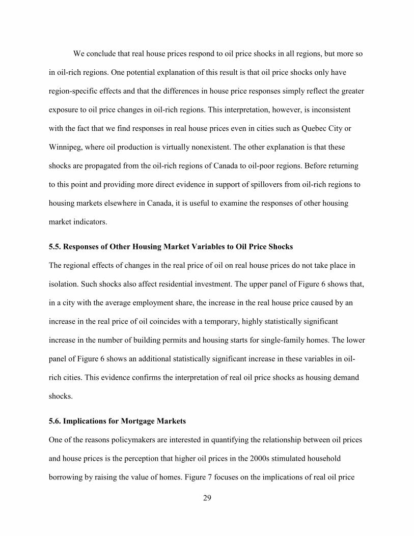
model. First, government revenues in oil-rich provinces increase in response to positive oil price

shocks by more than in other provinces, but government expenditures in oil-rich provinces

increase by no more than in other provinces, consistent with an effective redistribution of oil

income across provinces. Second, we provide evidence for slack in the labor market. Higher real

oil prices cause a persistent expansion in overall employment and a decline in the unemployment

rate in all regions. This effect is even more pronounced in the oil-rich regions. There is no

evidence of net migration from oil-poor provinces to oil-rich provinces in response to higher real

oil prices, however, consistent with the literature on regional labor demand shocks (e.g., Autor,

Dorn and Hanson 2013; Dix-Carneiro and Kovak 2017). Third, we show that real GDP increases

in response to higher real oil prices in all provinces, consistent with an increase in the domestic

demand for goods and services. Not only do we find increases in the value added of industries

that produce inputs for the oil sector (such as machinery or fabricated metals), but also increases

in the value added of industries not closely tied to the oil sector through the supply chain. These

industries are mostly located outside the oil-rich regions. Our evidence that these responses are

regionally homogeneous implies that the economic stimulus from higher oil prices is propagated

to virtually all sectors and regions of the economy.

Our analysis of Canadian housing markets contributes to the literature on the relationship

between housing markets and the macro economy, as well as to a growing literature on the

regional propagation of shocks. For example, Feyrer, Mansur and Sacerdote (2017) quantified

the spatial effects of county-level drilling shocks associated with the U.S. fracking revolution on

employment and income, and Allcott and Keniston (2018) conducted a similar analysis of the

effects of oil and gas booms on a range of economic outcomes including housing rents. Our

analysis is also related to Kehrig and Ziebarth (2017), who studied the effects of oil supply

5

shocks on U.S. regional labor markets, including the implications for real house prices, based on

regional differences in the dependence on oil as an input in production. Unlike in these earlier

studies, our primary focus is on the housing market. We also employ a different empirical

methodology and data set, we exploit a different source of cross-sectional variation, and we

provide new theoretical insights and new evidence on how oil price shocks are transmitted across

regions.

The remainder of the paper is organized as follows. In section 2, we estimate the effects

of shocks to the Canadian real price of oil at the national level based on structural VAR models.

Section 3 reviews the economic mechanisms that allow oil price shocks to affect Canadian

housing markets in all regions. Building on this discussion, we develop, in section 4, a

theoretical model of the propagation of real oil price shocks from oil-rich to oil-poor regions.

The implications of this model are empirically evaluated in sections 5 and 6. The concluding

remarks are in section 7.

2. The Effect of Oil Price Shocks on House Prices at the National Level

Canada is the fifth largest oil producer in the world. Most Canadian crude oil is exported, with

almost all oil exports going to the United States. Crude oil produced in Canada is priced in U.S.

dollars in global markets. Since Canadian housing demand is determined by real income

measured in Canadian consumption units, our baseline structural VAR model of the

determination of Canadian real house prices in section 2.1 expresses real oil price shocks in

Canadian consumption units. The real oil income generated in the oil-rich regions of Canada also

depends on the real exchange rate, however. Even if the global price of oil remained unchanged,

an exogenous change in the exchange rate would shift domestic income derived from oil

production and hence the demand for housing. In section 2.2, we address this concern by

6

showing that exogenous real exchange rate shocks are not an important source of the variation in

the Canadian real price of oil, which allows us to focus on shocks to the Canadian real price of

oil in the remainder of the paper.

2.1. The Effects of Shocks to the Canadian Price of Oil on National House Prices

As a first step, in this section we quantify the extent to which shocks to the real price of oil affect

national real house prices in Canada. The upper panel of Figure 1 shows the evolution of the

Teranet Canadian house price index, deflated by the consumer price index (CPI), as reported by

Statistics Canada.2 The lower panel of Figure 1 shows the Canadian real price of oil, obtained by

deflating the Canadian dollar price for Western Canadian Select (WCS) crude oil by the CPI.3

We analyze the relationship between these time series based on a monthly structural VAR(6)

model with intercept for ( ), , infl , , i ,t t t t t ty rpoil emp rhp= ∆ ∆ ∆ where trpoil∆ denotes the

percentage change in the Canadian real price of oil, temp∆ denotes the percentage change in

total employment, as reported by Statistics Canada, inflt denotes the rate of consumer price

inflation, trhp∆ denotes the percentage change in the real house price index, and it denotes the

5-year fixed mortgage rate quoted by major institutional lenders, as reported by the Canadian

Mortgage and Housing Corporation.4 The raw data cover March 1999 to August 2017. All data

have been seasonally adjusted.5

2The Teranet National Bank Composite 11 House Price Index is constructed by the repeat-sales method based on the rate of change in home prices in 11 Canadian metropolitan areas (Calgary, Edmonton, Halifax, Hamilton, Montreal, Ottawa, Quebec City, Toronto, Vancouver, Victoria, and Winnipeg). 3 The WCS price is the price for delivery at Hardisty, Alberta, expressed in Canadian dollars, and suitably extended back to 1999, as reported by the Canadian Association of Petroleum Producers. The WCS is representative of the types of crude oil produced in Canada. 4 This rate is the most common mortgage rate in Canada. Very similar results are obtained when using estimates of the corresponding average effective mortgage rate. 5 The lag order choice coincides with the estimate that would be obtained based on the Akaike Information Criterion with an upper bound of 12 autoregressive lags. Since the share of mining, quarrying, and oil and gas extraction in Canadian GDP has been nearly constant at about 8.5% since 1999, we do not model variation in this share.

7

The VAR model is identified recursively. Given that Canada is a small open economy,

we treat the percentage change in the real price of oil as predetermined with respect to the

Canadian economy.6 The real house price is allowed to respond to changes in employment and in

the inflation rate contemporaneously, but employment is considered too sluggish to respond

contemporaneously to unexpected changes in inflation, in real house prices, and in the nominal

lending rate. Likewise, we rule out feedback within the current month from real house prices to

consumer price inflation. The nominal mortgage rate is ordered last, allowing for the possibility

that the central bank may respond contemporaneously to house prices as well as inflation and

employment, thereby affecting the mortgage rate. By construction, the responses to real oil price

shocks are invariant to the ordering of the model variables below the real price of oil, and the

responses to mortgage rate shocks are invariant to the ordering of the model variables above the

mortgage rate. All impulse-response confidence intervals are constructed based on the

conditional heteroskedasticity-robust residual block bootstrap of Brüggemann, Jentsch and

Trenkler (2016).7

Figure 2 focuses on three key determinants of real house prices. An unexpected increase

in the real price of oil causes a statistically significant persistent increase in real house prices.

The initial drop in real house prices is consistent with inflation rising faster than nominal house

prices on impact. An unexpected increase in total employment also causes a statistically

significant persistent appreciation of real house prices, reflecting higher labor income and hence

higher housing demand. Finally, an unexpected increase in the nominal 5-year mortgage lending

6 This assumption is valid even for the much larger U.S. economy (Kilian and Vega 2011). 7 We do not differentiate between global oil demand and oil supply shocks. This distinction is neither necessary, as discussed in section 5.3, nor feasible in practice because it would require much larger-dimensional VAR models than can be estimated on our sample starting in March 1999. Even a two-step approach, as in Kilian (2009), that involves recovering the oil demand and oil supply shocks from an oil market VAR estimated on a larger sample, before projecting Canadian variables on current and lagged values of these shocks, would be infeasible in our case.

8

rate causes a statistically insignificant persistent decline in real house prices with a delay of one

quarter as the mortgage cost rises.8

Figure 3 examines the effects of an unexpected increase in the real price of oil on

Canadian macroeconomic aggregates. The estimates provide additional insights into the

transmission of an unexpected oil price increase to the housing market. National employment

increases persistently, consistent with an economic expansion and rising demand for housing in

response to higher real oil prices. There is only a short-lived increase in inflation. The nominal

lending rate increases persistently, which could be driven by the response of monetary policy or

by the higher demand for capital, as the economy expands. A variance decomposition based on

the estimated VAR model shows that real oil price shocks account for about 11% of the

variability in the growth rate in real house prices, which is a large share given the well-

documented difficulties of explaining time series variation in asset prices. In fact, it is distinctly

larger than the contribution of employment shocks (4%) and mortgage rate shocks (3%).

2.2. The Role of the Exchange Rate in Measuring Oil Price Shocks

The role of exogenous changes in the real exchange rate may be quantified by replacing the

Canadian real price of oil in the baseline recursive structural VAR(6) model of section 2.1 with

the real price of oil in U.S. consumption units and adding the Canadian real exchange rate as the

variable ordered last.9 This allows the real exchange rate to respond to all other shocks

contemporaneously. The residual shock is treated as a measure of exogenous real exchange rate

variation. As Figure 4 shows, an unexpected increase in the U.S. real price of crude oil has much

the same effect on employment, real house prices, inflation, and the mortgage rate as an 8 This result is consistent with evidence in Glaeser, Gottlieb and Gyourko (2010), among others, that the empirical relationship between U.S. house prices and interest rates is weak. 9 The nominal exchange rate data and the U.S. CPI are from FRED. The real price of Canadian crude oil in U.S. consumption units is measured by deflating the WCS price in U.S. dollars by the U.S. CPI, allowing for differences in the characteristics of Canadian crude oil from WTI or Brent crude oil (Kilian 2016).

9

unexpected increase in the Canadian real price of oil in Figure 3. Likewise, the share of the

variability of real house prices explained by these real oil price shocks is almost the same. This is

direct evidence that exogenous exchange rate fluctuations may be ignored for the purpose of our

analysis and lends credence to our approach of expressing the real price of oil in Canadian

consumption units in the remainder of the paper.

3. Determinants of the Response of Housing Markets to Canadian Real Oil Price Shocks

The evidence in section 2 suggests that oil price shocks have statistically significant effects at the

national level. It is not surprising that positive oil price shocks that represent income gains in oil-

rich regions would raise house prices and stimulate residential investment in these regions. It is

less obvious, however, to what extent these shocks are propagated to other regional housing

markets. In this section, we outline the channels by which real oil price shocks would be

expected to affect Canadian housing markets more broadly. We first review the channels through

which real oil price shocks may affect real income and hence the demand for housing and real

house prices, both in oil-rich and in oil-poor provinces. We then discuss how at the same time

higher real oil prices may reduce the demand for housing and lower real house prices through

other channels. These insights will be used in section 4 to build a theoretical model of the

regional effects of real oil price shocks that incorporates the empirically most relevant channels

and that explains why higher real oil prices on balance tend to be associated with higher real

house prices.

Over our sample period, as much as 78% of the crude oil produced in Canada is exported,

while the share of crude oil used by the Canadian economy is only 2% of GDP on average. We

therefore focus on the effects of oil price shocks on income and spending rather than on the cost

of domestic production, consistent with the conventional view of how oil price shocks affect the

10

economy (Kilian 2014).

3.1. How Higher Real Oil Prices May Cause Real House Prices to Increase

Since Canada historically has been a net exporter of crude oil, unexpected increases in the real

price of oil measured in Canadian consumption units imply that Canada as a whole receives

more real income. These real income gains, however, are not evenly distributed across the

country. Whereas households in oil-rich provinces such as Alberta, Saskatchewan, and, more

recently, Newfoundland and Labrador experience direct real income gains from higher oil prices,

households in oil-poor provinces do not. The income gains associated with real oil price

increases may be propagated to households in oil-poor provinces, however, by the government

redistributing income across provinces, by interprovincial trade, or by migration within Canada.

Government Redistribution. Oil production generates substantial revenues for provincial

governments through (i) taxes and royalties on oil production, (ii) property taxes, (iii) lease

payments, and (iv) fees for the use of public land. In Alberta, for example, oil and gas royalties

alone accounted for 28% of the provincial government revenue in 2008. Oil booms also raise

income tax revenue in oil-rich regions. These funds may be transferred to the federal government

and redistributed across provinces, providing an economic stimulus in oil-poor provinces that

increases housing demand and raises property values.10

Trade Between Provinces. An oil-poor province may also benefit from an oil boom in oil-rich

regions to the extent that higher demand for goods and services from oil-rich regions stimulates

10 Canada, in particular, has used this mechanism for many years. The Canadian “equalization payments” across provinces are based on a formula that calculates the difference between the per capita revenue yield that a particular province would obtain using average tax rates and the national average per capita revenue yield at average tax rates. For example, according to the Department of Finance in Canada, in 2016-17, the provinces with the largest oil sector, Alberta, Saskatchewan, Newfoundland and Labrador, and British Columbia, collectively transferred tax revenues equivalent to $2,573 per capita to Prince Edward Island, $2,259 per capita to New Brunswick, $1,822 per capita to Nova Scotia, $1,328 per capita to Manitoba, $1,206 per capita to Quebec, and $166 per capita to Ontario. The transfers received by the provinces can be spent in any way the provincial government desires.

11

aggregate real output. The strength of this effect depends on the magnitude of the consumption

stimulus from higher real incomes in the oil-rich region and on the degree to which oil firms rely

on inputs produced in oil-poor regions.

Migration Between Provinces. In addition, increases in the demand for labor in oil-rich

provinces caused by higher oil prices may stimulate net migration toward oil-producing regions.

This migration increases the demand for housing in oil-rich provinces and hence house prices. At

the same time, all else equal, housing demand in other provinces declines, resulting in lower

property values elsewhere in the country. This channel is not likely to be quantitatively

important, given the finding in the related literature on regional labor demand shocks that

regional labor mobility is low (e.g., Autor, Dorn and Hanson 2013; Dix-Carneiro and Kovak

2017). Indeed, our empirical analysis in section 6 confirms that there is no interprovincial net

migration to oil-rich provinces in response to oil price shocks.

Risk Sharing. Another potential channel of transmission is risk sharing, which occurs to the

extent that residents of oil-poor regions hold assets of companies in oil-rich regions and residents

of oil-rich regions hold assets of companies in oil-poor regions. Higher returns in oil assets, for

example, allow residents in oil-poor regions to partake in the real income gains in the oil sector.

The potential importance of risk sharing has been discussed in a variety of contexts.11 There are

two reasons to believe that this channel is unimportant within Canada. First, private ownership of

mineral rights is the exception. For example, close to 80% of the oil and natural gas rights in the

oil-producing provinces of Alberta and Saskatchewan are publicly owned and much of the

11 For example, Asdrubali, Sørenson, and Yosha (1996) document significant risk sharing across state borders in the United States that allows consumers to partially smooth state-level shocks. Kilian, Rebucci and Spatafora (2009) discuss risk sharing between oil-exporting and oil-importing countries at the global level. Fitzgerald and Rucker (2016) study the evidence that royalty income generated by U.S. shale oil producers is transmitted across state borders.

12

remainder is locally owned.12 Thus, few residents outside of the oil region generate income from

these rights. Second, as of 2012, more than two-thirds of Canadian oil sands production was

owned by foreigners, so the majority of oil industry profits was sent abroad rather than

supplementing Canadian incomes.13

3.2. How Higher Real Oil Prices May Cause Real House Prices to Fall

Although there are strong reasons to expect higher real oil prices to be associated with higher

real house prices, as discussed in section 3.1, there are also several countervailing forces,

including increases in consumer spending on fuel, environmental externalities of the oil booms

triggered by higher oil prices, a possible tightening of monetary policy in response to actual or

anticipated inflationary pressures from higher oil prices, and the appreciation of the Canadian

dollar in response to higher oil prices. Some of these channels can be shown to be quantitatively

unimportant, while others need to be incorporated into theoretical models of the regional

transmission of oil price shocks.

Consumer Spending on Fuel. One channel of transmission is changes in the cost of fuel both in

oil-rich and in oil-poor regions, as higher oil prices increase the cost of fuel, reducing the

household income available for other purchases (e.g., Edelstein and Kilian 2009). For example,

Larson and Zhao (2017) use a model incorporating changes in commuting costs to demonstrate

that real house prices fall in oil-poor cities and rise in oil-rich cities in response to higher real oil

prices. Thus, it is important to incorporate changes in the cost of fuel into models of the regional

12 Ownership information can be found in a range of government documents and publications by interest groups such as http://publications.gov.sk.ca/documents/310/93210-Disposition%20Types%20and%20Crown%20Public%20Offerings.pdf and https://www.fhoa.ca/about-freehold-mineral-rights.html. 13 See, e.g., “Majority of Oil Sands Ownership and Profits Are Foreign, Says Analysis,” Financial Post, May 20, 2012, https://business.financialpost.com/news/majority-of-oil-sands-ownership-and-profits-are-foreign-says-analysis.

13

transmission of real oil price shocks to the housing market.14

Environmental Costs. There is also evidence that the oil booms associated with higher oil

prices may create negative externalities that lower property values in oil-producing regions. One

reason is the environmental degradation associated with oil production. For example, the risks of

water contamination or other health hazards from oil production or oil spills have been

associated with lower property values, the inability to insure homes, and homeowners being

denied mortgages.15 Property values are also sensitive to local disamenities such as noise, traffic

congestion, nighttime lights, air pollution, or the visual blight of oil rigs, oil pipelines, and land

clearing. These effects, however, tend to be too local to be relevant for the transmission of oil

price shocks to housing markets at the city or province level.

Monetary Policy Reactions. Actual or anticipated inflationary pressures triggered by positive

oil price shocks may prompt the Bank of Canada to raise interest rates in response to higher oil

prices. To the extent that such short-term interest rate responses are passed through to the 5-year

mortgage rate, they may reduce the demand for housing and real house prices. Moreover, given

the evidence in Allen, Clark and Houde (2014), one might expect the mortgage rate responses to

oil price shocks to differ across regions. We abstract from monetary policy reactions in the

theoretical analysis in section 4 for two reasons. First, the results in section 2 show that the

mortgage rate responses to oil price shocks are too weak to offset the increase in real house

prices caused by higher real oil prices. Second, we find no statistically significant regional

14 In related work, Sexton, Wu and Zilberman (2012) show that an unexpected increase in the real price of crude oil increases the cost of commuting to work, lowering the real value of homes away from the city center and increasing foreclosure rates, as homeowners can no longer afford their mortgage payments. Molloy and Shan (2013) elaborate on this point, stressing the implications for housing demand and new housing construction. 15 Boxall, Chan and MacMillan (2005) document that property values in Alberta are negatively correlated with the number of sour gas wells and flaring oil batteries located in the vicinity of the property. Related work on the impact of the fracking boom on local housing markets in the United States includes Muehlenbachs, Spiller and Timmins (2015) and Cunningham, Gerardi and Shen (2017).

14

heterogeneity in the response of mortgage rates to oil price shocks.16 The latter result holds both

for insured mortgages – consistent with the findings in Hurst et al. (2016) for the United States –

and for uninsured mortgages.

Exchange Rate Effects. Finally, an exogenous shock to the real price of oil in global markets

causes both the real price of oil in Canadian consumption units and the Canadian real exchange

rate to appreciate, complicating the analysis because oil price shocks may affect Canadian real

income and hence real house prices both directly and through their effects on the competitiveness

of the tradable goods sector. The results in section 2.2, however, imply that the latter effects are

too small to offset the positive effect of higher global real oil prices on Canadian employment

and real house prices.

4. A Theoretical Model of the Regional and Sectoral Effects of Real Oil Price Shocks

This section introduces a stylized model of the regional transmission of real oil price shocks to

the housing market. Our model shares with standard urban models of the transmission of oil

price shocks to housing markets the insight that higher oil prices raise labor incomes in oil-rich

regions and hence raise real house prices, while the higher cost of motor fuel lowers the demand

for housing everywhere (e.g., Larson and Zhao 2017). Unlike these earlier studies, however, our

model incorporates three additional channels of transmission, namely interprovincial supply-

chain links, interprovincial trade in consumer goods, and the government redistribution of oil

income. We abstract from risk sharing and from the responses of migration and monetary policy

to oil price shocks for the reasons discussed in section 3. The objective of the theoretical analysis

is to shed light on the conditions under which real oil price shocks are transmitted to housing

markets in oil-poor regions, even in the absence of real exchange rate responses. Our model is

16 The average provincial mortgage rates were constructed based on quarterly proprietary loan-level micro data available to the Bank of Canada that provides information on the rate charged for each originated mortgage.

15

simple enough to be analytically tractable. The sign of the effect of an increase in the real price

of oil on real house prices in oil-rich and oil-poor regions, respectively, may be determined using

comparative statics.

4.1. Outline of the Model

Consider a country with an oil-producing region (region 1) and a non-oil-producing region

(region 2). All firms are representative. Oil is produced in region 1 by combining labor and

intermediate goods. The production of intermediate goods and consumption goods takes place in

region 2. Their production uses labor only. Within region 2, labor may be freely allocated

between the production of the intermediate good and the production of the consumption good.

The intermediate good is sold to the oil sector in region 1. Oil and the consumption good are

traded internationally. Any shortfall of these goods is met by imports. Any excess production is

exported.17 Since these goods are supplied elastically from abroad, their price is determined

internationally. The price of the consumption good is normalized to 1. The real price of oil is

exogenously given and is denoted by .p For simplicity, the cost of shipping goods domestically

or internationally is set to zero.

In each region { }1,2 ,i∈ representative households supply labor and are compensated at

the real wage rate, .iw Labor supply is inelastic in each region and immobile across regions.18

17 Since oil is primarily exported, our model implies that consumer goods are imported by the Canadian economy. This assumption is consistent with evidence that, with the exception of the aircraft industry, Canada primarily exports mineral, farm, forestry, fishing, and energy products. In contrast, the consumer goods industry, the chemical industry, the auto industry, and all other manufacturing industries are net importers, consistent with the model structure. 18 An alternative would have been to model households’ labor-leisure choices as endogenous under additional restrictions on the utility function. Such a model would imply a counterfactual reduction in employment in region 2 in response to higher real oil prices. The reason is that, when the government redistributes oil revenue from region 1 to region 2, the windfall income gain in region 2 causes a reduction in labor supply and, hence, in total employment, which is at odds with the data.

16

The supply of labor in region 1 is fixed.19 In region 2, labor supply may be fixed or,

alternatively, there may be slack in the labor market, which is represented as the labor supply in

region 2 being an increasing function of .p Households purchase housing services and the

consumption good. Consumption and housing services are assumed to be complements. The

government redistributes wealth from the oil-rich region to the oil-poor region based on a tax on

oil producers’ revenue, which is in part spent on consumer goods and in part redistributed

directly to households in region 2, adding to their income. Workers commute to work in both

regions. The cost of motor fuel depends linearly on .p

Housing services are produced from land and capital.20 As in Davis and Heathcote

(2007), capital represents the value of physical structures. Land is in fixed supply. The

endogenously determined real price of housing services in region i is denoted by .iq Since

house prices in region , ,ii hp can be expressed as the discounted sum of all future prices of

housing services, we focus on the determination of .iq 21

4.2. Region 1: Oil-Producing Region

Firms: Oil-producing firms are competitive and take p as given. Their technology is constant

returns to scale (CRS). Oil is produced from intermediate goods, ,M supplied by region 2 and

regionally supplied labor, 1.N Let 1( , )O N M denote the output of oil in region 1, where 1N is

the total labor supply in region 1. The two inputs are complements, which implies that

21 0.O N M∂ ∂ ∂ > The government imposes a revenue tax at rate τ on oil revenue. Oil firms

19 This simplifying assumption could be relaxed without affecting the signs of the responses to real oil price shocks in region 1. 20 Although labor is an important input in building homes and apartments, it is not a major input in the production of housing from existing dwellings and is not considered in most urban models (Yinger 2015). 21 For example, in the standard user cost model discussed in Glaeser, Gottlieb and Gyourko (2010) the house price is proportionate to the price of housing services.

17

choose labor 1N and M to maximize 1(1 ) ( , )pO N Mτ− − 1 1 ,Mw N p M− where Mp denotes the

price of the intermediate good. From the first-order conditions for profit maximization,

1 11

(1 ) ( , ),Ow p N MN

τ ∂= −

∂ (1)

1(1 ) ( , ).M Op p N MM

τ ∂= −

∂ (2)

Housing Service Providers: Our model allows both the price and the quantity of housing

services to adjust to housing demand shocks. Housing services are produced from land and

capital using a CRS technology. The competitive providers of housing services in region 1

choose land, 1,L and capital, 1K , to maximize ( )1 1 1 1 1 1 1, ,L Kq H L K r L r K− − where 1H denotes the

quantity of housing services provided in region 1, 1Lr is the rental rate of land, and Kr is the

rental rate of capital, which is assumed to be constant and determined in international capital

markets. The fixed quantity of land in region 1 is owned by the households in region 1. Profit

maximization implies that

( )1 1 11 1

1

,,L H L K

r qL

∂=

∂ (3a)

( )1 1 11

1

,.K H L K

r qK

∂=

∂ (3b)

Since Kr and 1L are constant, equation (3b) implies that 1 1 0.K q∂ ∂ > Given the solution for

1 1( )K q from equation (3b), equation (3a) determines 1Lr for given 1.q In addition, the production

function for housing services implies that the housing supply curve is upward sloping, i.e.,

1 1 0.H q∂ ∂ > The functional form of ( )1 1 1,H L K is general enough to accommodate differences

in housing supply elasticities across regions. A smaller housing supply elasticity, all else equal,

implies a larger response of real house prices to a housing demand shock.

18

Households: Households in region 1 choose their consumption ( 1c ) and housing services ( 1h ) to

maximize utility 1 1( , )U c h subject to 1 1 1 1 1 1 1 1 1( ) ,Lc q h w n r q L k p+ = + − where 1n is the fixed labor

supply, 1k is a constant that reflects the inelastic demand for fuel, 1k p is the cost of fuel, and

1 1Lr L is the rental income from land. We assume that the utility function is concave and twice

differentiable. Using equation (1) and the equilibrium condition in the labor market, the budget

constraint can be expressed as

11 1 1 1 1 1 1 1 1 1

1

( , )(1 ) ( ) ( , ),LO N Mc q h N k p r q L I p qN

τ ∂

+ = − − + ≡ ∂

where 1 1( , )I p q denotes household income. The first-order condition for 1h implies that

( ) ( )1 1 1 1 1 1 1 1 1 1 1( , ) , ( , ) , 0.c hq U I p q q h h U I p q q h h− − + − =

In equilibrium, housing demand 1h equals housing supply 1 1( ),H q which allows us to derive the

change in the equilibrium price of housing services in response to a change in the price of oil. By

the implicit function theorem,

( )

11 1 1

1 1 1 11 1 1 1

1 1 1 1

( , ) ,cc ch

cc ch c ch hh

q U Uq I p qp pH I H Hq U U H q U q U U

q q q q

− +∂ ∂=

∂ ∂ ∂ ∂ ∂ ∂− + + − + + − ∂ ∂ ∂ ∂

(4)

where 1 1 1 1 1 1 1 1 0KH q H q I q r K q+ ∂ ∂ −∂ ∂ = ∂ ∂ > from the definition of 1,I the zero profit

condition for housing service providers, and the assumption of CRS. Since wage income exceeds

the cost of fuel in the data, ( )1 1 1 1 1( , ) / 0I p q p w n k p p∂ ∂ = − > for suitably chosen parameters. It

follows that 1 0q p∂ ∂ > (and hence 1 0).hp p∂ ∂ > Equation (4) also implies that the smaller the

own-price elasticity of housing supply, the greater the response of the price of housing services

to the oil price. Moreover, consumption also increases in response to higher oil prices,

19

1 1 1 1 1 1 11 1

1 1

( , ) ( , ) 0,c I p q H I p q qH qp p q q p

∂ ∂ ∂ ∂ ∂= − + − > ∂ ∂ ∂ ∂ ∂

because equation (4) implies that ( )1 1 1 1 1 1 1 1 1 1( , ) ( , ) .H q H q I p q q q p I p q p+ ∂ ∂ − ∂ ∂ ∂ ∂ ≤ ∂ ∂

4.3. Region 2: Non-Oil-Producing Region

Firms: There are two types of competitive firms in region 2. Firms that produce the intermediate

good employ labor, 2 ,MN to maximize 2 2M M Mp M w N− subject to 2 ,MM aN= where a denotes

labor productivity in the intermediate goods sector. Profit maximization implies 2 .M Mw p a=

Firms that produce the consumption good choose 2CN to maximize 2 2

C CC w N− subject to

2 ,CC bN= where b denotes labor productivity in the consumer goods sector. Profit maximization

implies 2 .Cw b=

Since there are no frictions, workers in region 2 are indifferent to working in either

industry. Thus, the real wage must be equal. Given 2 2 2M Cw w w= = ,

/ .Mp b a= (5)

Hence, oil producers in region 1 can expand their production without driving up the price of

intermediate goods. The quantity of the intermediate good is determined by equations (2) and

(5):

1/ (1 ) ( , ).b a p O M N Mτ= − ∂ ∂ (6)

Since the labor supply in region 1 is fixed, equation (6) determines M as a function of .p By the

implicit function theorem, the production of intermediate goods increases with the oil price,

0M p∂ ∂ > , and, hence, so does employment in this sector, 2 0.MN p∂ ∂ > In other words, our

model implies that, as the oil sector in region 1 expands, so does the intermediate goods sector in

20

region 2.

Housing Service Providers: The structure of this market resembles that in region 1 with suitable

changes in notation.

Households: The government redistributes a fraction ω of the oil tax revenue pOτ to

households in region 2. Households in region 2 earn wage 2 ,w b= receive the lump-sum transfer

,pOωτ and choose 2c and 2h to maximize 2 2( , )U c h subject to 2 2 2c q h+ =

2 2 2 2 2 2( )Lw n r q L k p pOωτ+ − + ≡ 2 2( , ),I p q where 2 2 2 .M Cn n n= + After imposing the labor market

equilibrium condition, the budget constraint may be expressed as 2 2 2 2 2 2 2( ) ( )Lc q h bN p r q L+ = +

2( ) ,O k pωτ+ − where 2 ( )N p is the endogenous total labor supply in region 2. Note that

2 2 22

( , )I p q N Ob O p kp p p

ωτ ∂ ∂ ∂

= + + − ∂ ∂ ∂

is positive as long as the additional labor income and the additional government transfer received

by the household exceed the additional cost of fuel:

22

( ) ,N p Ob p O kp p

ωτ ωτ∂ ∂+ + >

∂

where 2 ( ) 0.N p p∂ ∂ ≥ In that case, housing rents, house prices, and consumption increase.

4.4. Summary of the Model Implications

In one version of the model, 2 ( ) 0N p p∂ ∂ = and full employment holds; in the other version,

2 ( ) 0,N p p∂ ∂ > representing slack in the labor market. Depending on which of these

assumptions holds, the model implications for region 2 differ substantially. The first version of

the model treats labor supply as fixed in all regions. It implies that in the absence of government

redistribution of oil revenue across regions, the effect on consumption and real house prices is

21

positive in the oil-rich region, but negative in the oil-poor region. Supply-chain linkages alone

are not enough to raise real house prices in the oil-poor region because the expansion of the

intermediate goods sectors comes at the expense of the consumer goods sector. Since aggregate

real output and employment remain unchanged, so does labor income. Net income falls as fuel

costs rise. Only sufficient redistribution of oil income to the oil-poor region by the government

will reverse this negative sign.

In contrast, in the second version of the model, the labor supply curve in region 2 shifts to

the right as the real price of oil increases. As a result, higher demand for intermediate goods and

consumer goods by the oil-rich region raises aggregate real output and employment in the oil-

poor region, even in the absence of government redistribution. As long as the sum of additional

oil tax transfers and additional labor income in the oil-poor region exceeds the additional cost of

fuel, real output, consumption, and real house prices will increase in region 2. Unlike in the

previous version of the model, employment and real output in the consumer goods sector in the

oil-poor region need not contract, but may expand along with the intermediate goods sector.

The next two sections empirically evaluate these model predictions based on panel

regression models estimated on quarterly city- and province-level data, respectively. Section 5

focuses on the effects of oil price shocks on the regional housing markets, while section 6

considers the implications for employment, real output, and net migration. We provide evidence

that the version of the model with flexible labor supplies provides a better fit to the data.

5. The Responses of Regional Housing Markets to Oil Price Shocks

Regions in our empirical analysis may refer to provinces or cities. Our data set consists of 33

cities, defined as metropolitan areas having at least 100,000 residents, and 9 provinces,

22

respectively.22 We focus on the provinces of Alberta, British Columbia, Newfoundland and

Labrador, Nova Scotia, New Brunswick, Quebec, Ontario, Manitoba, and Saskatchewan, which

account for 99.2% of the Canadian population. Our analysis is mainly conducted using city-level

data at quarterly frequency. We use provincial data only when city-level data do not exist.23

5.1. Regional Data

Our primary interest is the response of regional real house prices to oil price shocks. Quarterly

city-level house price indices are constructed based on the average growth rate of the quarterly

house price index across all Forward Sortation Areas (FSA) within a city.24 The FSA-level house

price indices are reported by Teranet-National Bank and are based on the repeat-sales method.

Quarterly provincial data for house prices are constructed by averaging the monthly average sale

price by province published by the Canadian Real Estate Association (CREA). All nominal data

are deflated using the appropriate provincial CPI from Statistics Canada. We also consider a

range of other quarterly and annual outcome variables ranging from housing and mortgage

market indicators to employment, real activity, government revenue, and government spending

that are useful in evaluating the predictions of the theoretical model.25

5.2. Empirical Strategy

Our panel regression analysis focuses on the period 1999Q2–2017Q2, consistent with the time

22 A precise definition of Census Metropolitan Areas (CMAs) can be found in the Census Dictionary of Statistics Canada. 23 For example, city-level data on real gross domestic product (GDP) are only available after 2009 and there are no sectoral real GDP data at all at the city level, so we use province-level data. Likewise, quarterly data on residential mortgage loans and personal loans by banks and annual data on government expenditures and revenues are only available at the province level. 24 The only exception is four cities in New Brunswick and Saskatchewan, for which no FSA data are available. We use house price data from CREA for these cities. 25 The data for city-level employment, the unemployment rate, the number of residential building permits, and the number of housing starts are all from Statistics Canada. Data on the arrear rate are obtained from the Canadian Bankers Association. Quarterly chartered bank mortgages and personal loans by province, quarterly interprovincial migration, quarterly population by province, annual provincial government expenditures and revenues, and annual provincial real GDP and real GDP classified by the North American Industry Classification System (NAICS) are all from Statistics Canada.

23

series analysis in section 2. In estimating the response of real house prices (and other outcome

variables) to Canadian real oil price shocks, we exploit two sources of variation: the variability in

the real price of oil over time and the cross-sectional variation in the importance of the oil sector

for the regional economy.

We measure cross-sectional differences in the exposure of regions to oil price shocks by

the region-specific employment share of the oil sector or the region-specific share of the oil

sector in value added prior to the shock. By allowing the shares to vary over time rather than

fixing them at their average values, we capture changes in the importance of the oil industry in

each region over time. At the city level, there is no alternative to using employment shares. In

practice, the employment share is defined as the most recent two-quarter moving average of the

employment share for “mining, quarrying, and oil and gas extraction,” which represents the

finest sectoral disaggregate of the employment data available. Figure 5 shows the standardized

employment share weights for Calgary in Alberta, Saskatoon in Saskatchewan, and Vancouver in

British Columbia. It documents substantial variation in the importance of the oil industry across

cities and over time, which helps identify the regional responses to real oil price shocks.

At the province level, we instead interact real oil price changes with the share of “mining,

quarrying and oil and gas extraction” in provincial value added prior to the change in the real

price of oil. The value-added share for Alberta, for example, rose from 19% in 1999 to a peak of

33% in 2005, before declining back to 17% by 2016, reflecting the rise and decline of the oil

sands industry. In contrast, the value-added share for Ontario remained at approximately 1%

throughout the estimation period.26

26 The estimates at the province level are generally robust to the choice of the share measure, when both are available. The main substantive difference is that the value added share tends to produce more statistically significant estimates for government spending and revenues, which is expected since the latter respond to oil tax revenues rather than oil sector employment.

24

Our empirical strategy exploits the interaction of time series variation in real oil prices

with cross-sectional variation in regions’ exposure to the oil sector, in the spirit of Bartik (1991).

Because we are making use of a comparatively clean source of exogenous variation, as discussed

later, the causal effects of changes in the real price of oil can be estimated using the panel

regression model,

3

, 0 1 2 , 3 , ,1

,h h h h h h h h hi t t t i t h i t h q q i i t

qy p p s s Dβ β β β δ γ ε− −

=

∆ = + ∆ + ∆ × + + + +∑ (7)

where ,h

i ty∆ denotes the percent change between quarters t h− and t in the economic outcome

of interest (say, the real house price) in region ;i htp∆ denotes the percent change in the real

price of oil over the same period; ,i t hs − denotes the standardized employment share (or value

added share) prior to the change in the price of oil; , 1, 2,3,qD q = denotes a quarterly seasonal

dummy variable; and iγ denotes a set of regional fixed effects that absorb any time-invariant

heterogeneity. The error term ,hi tε denotes idiosyncratic shocks specific to region .i

Given that ,i t hs − is predetermined, the total causal impact of an increase in the real price

of oil on real house prices in region i over horizon h is captured by

1 2 , ,h hi t hsβ β −+ (8)

where 1hβ denotes effect in a region with , 0,i t hs − = and 2 ,

hi t hsβ − the region-specific effect that

depends on the importance of the oil sector for the regional economy, as measured by departures

of the share from zero.27

27 As an additional robustness check, we replaced h

tp∆ in equation (7) by quarterly fixed effects that absorb all common shocks at the aggregate level. The resulting time fixed-effects model, , 0 2 ,

h h h hi t t i t hy p sβ β −∆ = + ∆ × +

3 , , ,h hi t h i t i tsβ γ δ ε− + + + produced very similar estimates of 2 .hβ We therefore report only the estimates of model (7).

25

The standard errors are clustered at the regional (city or province) level. Because the

number of clusters is small in our analysis, conventional cluster-robust asymptotic standard

errors are not valid. Throughout the paper, we therefore report fixed-design wild bootstrap

p -values for 1̂hβ and 2

ˆ hβ clustered at the regional level, as discussed in Cameron, Gelbach and

Miller (2008).28

5.3. Identification of Causal Effects

The causal interpretation of 1hβ and 2

hβ rests on the assumption that changes in the real price of

oil are exogenous with respect to the Canadian economy, that they are unpredictable, and that

they are not correlated with exogenous changes in other variables that affect the Canadian

economy. These assumptions make sense for the following reasons.

As to the first condition, Canada is a small open economy, so Canadian demand for oil

does not affect the global price of oil. Moreover, since Canadian oil producers account for only

4% of world oil production, they are too small to influence the global price of oil and take the

price of oil as exogenously given.

As to the second condition, recent research shows that consumers treat the current real

price of oil as the best predictor of the future real price of oil (see, e.g., Anderson et al. 2011;

Anderson, Kellogg and Sallee 2013; Alquist, Kilian and Vigfusson 2013). Since there is no

evidence that firms are better at predicting the price of oil than households, we postulate that

firms and consumers alike perceive all changes in the real price of oil as permanent shocks.

As to the third condition, one concern is that some exogenous shock may shift both the

The advantage of model (7) compared with the time fixed-effect panel model is that it allows us to assess the total effect of changes in the real price of oil on each region. 28 Because the number of clusters is small, the fixed effect cannot be estimated consistently, invalidating conventional bootstrap confidence intervals and standard errors. Asymptotically valid p -values may be constructed by bootstrapping the model under the null hypothesis of zero coefficients (Canay, Santos and Shaikh 2018).

26

real price of oil and other variables affecting the Canadian economy, violating the all-else-equal

premise of causal inference. For example, increases in the real price of oil associated with an

exogenous boom in the global economy emanating from emerging Asia may be correlated with

increases in the real price of other Canadian export commodities. Our analysis of the Canadian

merchandise trade balance, however, shows not only that oil accounts for the bulk of Canadian

net export earnings, but that there is little comovement between the price of oil and the prices of

other important export commodities (such as lumber) during our estimation period, allowing us

to abstract from this concern. Likewise, Canadian manufactured exports do not appear to

increase systematically during the global economic boom of the 2000s, suggesting that demand-

driven real oil price increases are not associated with a direct stimulus for the Canadian

economy.

A related concern is that the Chinese economic boom of the 2000s may have been

associated both with an increase in the real price of oil and with increasing purchases by Chinese

real estate investors in Canada. Housing market data, however, show that foreign home owners

account for less than 1% of home ownership in most Canadian cities. Only in Vancouver and

Toronto is this share higher with 2.6%.29 Our results are robust to excluding Vancouver and

Toronto from the panel regressions, indicating that this additional link, if it exists, is not

quantitatively important.

Yet another concern is that the increased global demand for crude oil and other industrial

commodities in the 2000s coincided with the increased availability of inexpensive consumer

goods imports from emerging Asia, representing a favorable terms-of-trade shock, as Canadian

import prices dropped. Our VAR analysis, however, suggests that this effect must be small,

29 Source: Canada Mortgage and Housing Corporation: https://www.newswire.ca/news-releases/non-resident-ownership-of-condo-apartments-remains-low-and-stable-cmhc-665176373.html.

27

because a positive real oil price shock permanently raises the level of Canadian consumer prices

(see Figure 3).

A final concern is that exogenous oil supply disruptions caused by wildfires, power

outages, or unexpected oil pipeline shutdowns in Canada may simultaneously affect the real

price of Canadian crude oil and real house prices in Canada. There are three such events in

particular: The wildfire near Fort McMurray in Alberta in May 2016, the power outage in the

same area in mid-2018, and a shutdown of the Keystone pipeline from Canada to the United

States following a pipeline rupture in South Dakota in November 2017. The pipeline shutdown

and power outage occurred after the end of our sample. Events such as these do not undermine

our identification. First, none of these events occurred close to a city. Notably, Fort McMurray is

not included in our sample of Canadian cities because its population is too small. Second, even a

shutdown of 10% of Canadian oil production for two months has a negligible effect on annual

real value added in Canada and in Alberta, given the comparatively low share of the oil sector in

GDP. This fact limits the effects of such events on labor income and housing demand outside of

Fort McMurray. Third, our panel regression results are robust to terminating the sample after

2016Q1 (before the wildfire) and to including 2016Q2 dummies for all cities in Alberta.

5.4. Responses of Regional House Prices to Oil Price Shocks

Figure 6 shows the values of 1̂hβ and 2

ˆ hβ obtained from quarterly city-level data by estimating

equation (7) separately for each h and each dependent variable. Estimates that are statistically

significant at the 5% level are marked as filled circles and estimates that are significant at the

10% are marked as empty circles. For a city with a zero standardized employment share, the

estimate of 1hβ for real house prices is slightly negative at quarterly frequency, because nominal

house prices are sticky and inflation rises in the short run. At lower frequency, real house prices

28

increase steadily in response to an increase in the real price of oil, and the response becomes

statistically significant. The cumulative effect approaches 0.03 percentage points for annual

growth rates and 0.06 percentage points for biennial growth rates. The corresponding estimates

of 2hβ show that oil-rich cities experience an additional increase in real house prices in response

to higher real oil prices (and oil-poor cities a correspondingly smaller increase), but this

incremental response is more gradual, reaching 0.03 percentage points when using biennial

growth rates. The estimates of 2hβ are statistically significant at the 10% level at lower

frequency.30

Our estimates allow us to assess the total impact of real oil price shocks on each regional

housing market based on equation (8), controlling for the importance of the oil sector at each

point in time. To illustrate the regional heterogeneity in the propagation of oil price shocks,

consider the example of two cities: Vancouver with a standardized employment share near -0.6

in 2008Q2 and Calgary with a standardized employment share in excess of 3. From equation (8),

the resulting total effect of a positive 1% real oil price shock on real house prices in Calgary is a

0.03% increase based on annual growth rates and a 0.16% increase based on biennial growth

rates, whereas the total effect on real house prices in Vancouver is a 0.03% increase and a 0.04%

increase, respectively. Despite this heterogeneity, we find that, even for the lowest standardized

employment share, the effect of real oil price shocks on real house prices remains positive.31

30 We also experimented with an alternative model specification that allows for asymmetric responses to changes in the real price of oil. We examined the alternative hypothesis that a decline in the real price of oil lowers house prices beyond the effect associated with any percent change in the real price of oil. To minimize the risk of data mining across horizons we focused on the two-year horizon. There was no statistically significant asymmetry in the response of real house prices for either 1

hβ or 2 .hβ 31 An additional, empirically testable implication of the theoretical model in section 4 is that, if there are multiple cities within a region, all else equal, the cities with a less elastic housing supply should experience higher house price growth in response to a positive oil price shock. Since we are not aware of a well-established measure for the Canadian housing supply elasticity at the city level, comparable to the estimates for U.S. metropolitan housing markets in Saiz (2010), we leave this question for future research.

29

We conclude that real house prices respond to oil price shocks in all regions, but more so

in oil-rich regions. One potential explanation of this result is that oil price shocks only have

region-specific effects and that the differences in house price responses simply reflect the greater

exposure to oil price changes in oil-rich regions. This interpretation, however, is inconsistent

with the fact that we find responses in real house prices even in cities such as Quebec City or

Winnipeg, where oil production is virtually nonexistent. The other explanation is that these

shocks are propagated from the oil-rich regions of Canada to oil-poor regions. Before returning

to this point and providing more direct evidence in support of spillovers from oil-rich regions to

housing markets elsewhere in Canada, it is useful to examine the responses of other housing

market indicators.

5.5. Responses of Other Housing Market Variables to Oil Price Shocks

The regional effects of changes in the real price of oil on real house prices do not take place in

isolation. Such shocks also affect residential investment. The upper panel of Figure 6 shows that,

in a city with the average employment share, the increase in the real house price caused by an

increase in the real price of oil coincides with a temporary, highly statistically significant

increase in the number of building permits and housing starts for single-family homes. The lower

panel of Figure 6 shows an additional statistically significant increase in these variables in oil-

rich cities. This evidence confirms the interpretation of real oil price shocks as housing demand

shocks.

5.6. Implications for Mortgage Markets

One of the reasons policymakers are interested in quantifying the relationship between oil prices

and house prices is the perception that higher oil prices in the 2000s stimulated household

borrowing by raising the value of homes. Figure 7 focuses on the implications of real oil price

30

shocks for mortgage markets. Based on data at the province level, higher real oil prices cause a

declining percentage of mortgages in arrears, as well as increased consumer borrowing and rising

mortgage values. The pattern of these responses mirrors that of the responses of real house

prices. This fact suggests that Canadian households borrow against their home equity and

accumulate debt in response to higher oil prices. There is no statistically significant regional

heterogeneity in the responses of these financial variables.32

6. How Do Oil Price Shocks Propagate Across Regions?

In this section, we provide direct evidence that oil price shocks that generate direct income gains

in oil-producing regions are propagated to non-oil-producing regions, causing real house prices

to increase in all regions. We study the responses of a range of additional outcome variables

based on the panel regression model (7). The choice of these variables is guided by the

theoretical model in section 4. In section 6.1, we show that overall employment increases in

response to higher real oil prices in all regions, even in regions where oil production is virtually

nonexistent. This result supports the version of the theoretical model that allows for shifts in the

labor supply in response to higher oil prices. In section 6.2, we show that the real output of

industries that support the oil sector expands as the real price of oil price increases, consistent

with the model implication that supply-chain linkages are one of the propagation channels. In

addition, the real output of many industries that are not directly related to oil production also

increases, reflecting higher consumer demand and higher government purchases financed by oil

tax revenues. The latter channel is explored in more detail in section 6.3. Although our

regression framework does not allow us to quantify the contribution of these channels separately,

32 The mortgage value responses are based on a shorter sample ending in 2011Q2, given a major change in the definition of mortgage values, as reported by banks, which results in a discontinuous jump in mortgage values in 2011Q3.

31

it provides direct empirical support for the importance of each of these channels in propagating

regional shocks.

6.1. Regional Labor Market Responses

As the demand for goods produced in region 2 increases, the unemployed in that region are more

likely to find gainful employment, while individuals who had left the labor force at an earlier

stage may choose to return to the labor market in their region. As employment and labor income

rise, so does the demand for housing. Figure 8 examines the labor market responses to positive

real oil price shocks based on quarterly city-level data. The upper panel confirms that cities with

an average oil employment share experience an increase in real house prices, a persistent decline

in the unemployment rate, and an increase in employment. There is also a small but statistically

significant increase in oil employment in response to higher real oil prices.33 Based on equation

(8), even for the city with the lowest standardized employment share, the effect of a positive oil

price shock on total employment is positive. For oil-rich provinces, there is an additional decline

in the unemployment rate and an additional increase in total employment and in oil employment,

as shown in the lower panel of Figure 8.34

6.2. Regional Migration Responses

Another possibility not considered in the theoretical analysis is that the labor supply in region 1

may increase as a result of net migration from oil-poor provinces. Additional regression analysis

in the appendix, however, shows that increases in the real price of oil do not cause net migration 33 This increase is expressed as a share of total employment prior to the real oil price increase, since oil employment is small. 34 Further regression results (not shown to conserve space) show that the responses of the labor force are similar to those for employment, suggesting that workers who previously left the labor force choose to return in response to better employment opportunities. Average hours worked increase in oil-rich provinces, but not elsewhere. The nominal wage increases everywhere, but more so in oil-rich provinces. The real wage, however, increases in oil-rich provinces only. These results are consistent with increases in employment being made possible by a combination of reductions in unemployment and increases in the labor force, which helps alleviate the upward pressure on the real wage.

32

into oil-rich provinces, which motivates the exclusion of the migration channel from the model

in section 4 (see Figure A1).35 Our point is not that there has not been substantial interprovincial

net migration into the Canadian oil provinces since 1999, but that the evolution of this net

migration over time is not explained by changes in the real price of oil. As the appendix shows,

the latter result is not surprising, given that net interprovincial migration to Alberta dropped

sharply in 2007-08, amidst severe labor shortages, while the real price of oil rose dramatically.

At the same time, net migration to Sasketchawan increased dramatically well before the 2007/08

surge in the real price of oil, but dropped sharply, when the oil price surged (see Figure A2).36

It should be noted that the migration data underlying our analysis reflect the change in the

tax residency of individuals. They do not include oil-sector workers who spend only part of the

year working in oil-rich regions. Such temporary migrant workers have to declare their

employment in the oil sector in the oil-poor region where they officially reside. The right panel

of Figure 8, however, implies that oil employment in oil-poor regions does not increase in

response to higher oil prices, suggesting that temporary migration is not important. This

conclusion is also consistent with data on aircraft movements in and out of major Canadian

metropolitan area airports from Nav Canada, the company operating the Canadian civil air

navigation system.37 We find no evidence that the number of aircraft going into oil-rich cities

increases at a faster rate in response to higher real oil prices than the number of aircraft going

into other cities (see Figure A3).

35 In related work, Kehrig and Ziebarth (2017) provided evidence in a different context that regional migration in the United States increases in response to oil supply shocks. Their study, however, focused on in-migration rather than net migration. We also find evidence of statistically significant positive coefficients for in-migration, but these effects are offset by the positive coefficients for out-migration, resulting in statistically insignificant coefficients for net migration that are close to zero. 36 “Recent Migration Trends in Census Divisions: Fort McMurray, Calgrary and Edmonton,” Government of Alberta, Demographic Spotlight, March 2011, https://open.alberta.ca/dataset/6a962a43-f03d-4028-bc88-13391a8c71d4/resource/55750587-fd42-4823-8a69-354758ba67eb/download/2011-0311-migration-trends-fort-mcmurray-calgary-edmonton.pdf. 37 The flight data were obtained from Statistics Canada.

33

Finally, our response estimates are consistent with census data on regional migration

patterns that show that the majority of migrants living in Edmonton and Calgary arrived from

within the same province, from other oil provinces, or from abroad (e.g., Amirault, de Munnik

and Miller 2013). Data for the oil town Fort McMurray, for example, suggest that about half of

the migrants to Fort McMurray are from within Alberta, 17% are from the oil province

Newfoundland and Labrador, and about 10% are foreigners, leaving at most one in five migrants

from any of the oil-poor provinces.

6.3. Responses of Regional Real Output

The version of the model in section 4 with flexible labor supplies predicts an increase in real

output in both regions in response to an increase in the real price of oil. The first row of Table 1

shows estimates of 1hβ and 2

hβ for annual and biennial real GDP growth at the province level.38

Like the employment responses in section 6.1, the responses of aggregate real GDP are

statistically significant and positive for all provinces, even those with the lowest exposure to the

oil industry. This evidence corroborates the conclusions based on the labor market data and

strengthens the empirical support for the assumption of flexible labor supplies. The economic

expansion caused by positive real oil price shocks strengthens at longer horizons for oil-rich

provinces, but weakens for oil-poor provinces, suggesting that the economic expansion in oil-

poor provinces is comparatively short-lived. Next, we examine in more detail the empirical

support for the interprovincial trade channels of the transmission of oil price shocks to oil-poor

regions highlighted in the theoretical analysis. We start with the role of supply-chain linkages

and then examine the role of higher consumer demand.

38 The raw data are annual. All sectoral responses have been expressed as a share of real GDP prior to the real oil price increase, since in many provinces the value added of one type or another is so small that percentage changes in sectoral value added paint a misleading picture when comparing across provinces.

34

6.3.1. The Role of Supply-Chain Linkages

The flexible labor-supply version of the model in section 4 implies that the intermediate goods

sector should expand, but that the consumer goods sector may expand or fall, depending on the

strength of the regional transmission mechanism. Verifying the model prediction about increased

growth in the intermediate goods sector in response to higher oil prices is difficult because we do

not know the extent to which a given sector provides intermediate goods for oil-rich regions. In

Table 1 we present results for the mining sector and for the manufacturing sector, which,

according to the analysis in Allcott and Keniston (2018), account for most of the inputs supplied

to the oil sector.

As expected, Table 1 shows a tightly estimated positive response of mining, quarrying,

and oil and gas extraction, along with activities that directly support these industries. We also

find highly statistically significant increases in the annual growth rates of a broad range of

manufacturing activities that are related to oil production, with little or no evidence of regional

heterogeneity in this response, as measured by the absence of statistically significant 2ˆ hβ values.

This pattern is inconsistent with the hypothesis that the economic stimulus should be stronger in

oil-rich regions in the absence of regional spillovers, providing direct support for the existence of

spillovers from oil-rich to oil-poor regions. In fact, Table 1 shows that manufacturing responds

more strongly in oil-poor regions than in oil-rich regions, given that 12

ˆ 0.yrβ < Thus, there is

strong evidence in support of the supply-chain links highlighted in the theoretical analysis. In the

biennial data, the responses of several of the components of manufacturing value added remain

statistically significant, but not the overall response.

6.3.2. The Role of Higher Consumer Demand

Table 2 shows the annual value added in the remaining sectors of the economy exhibits a

35

statistically significant positive response to higher oil prices. The first three rows focus on

wholesale trade, retail trade, and transportation and warehousing. The highly statistically

significant responses in wholesale and retail trade, in particular, across all provinces are

consistent with an increase in consumer demand, as predicted by the theoretical model. The next

seven rows focus on the service sector. Again, there is a pattern of positive and statistically

significant responses across the board and little or no evidence of regional heterogeneity,

providing evidence of spillovers across regions. The particularly strong response of professional,

scientific, and technical services suggests that this sector provides additional support services for

the oil industry in response to higher oil prices.

The positive response of construction may reflect the increase in residential housing

demand, but could also be indicative of increased demand for roads and industrial infrastructure,

while the positive response of utilities suggests increased demand for water and power. Finally,

the positive response of public administration services in all provinces is suggestive of increases

in government spending driven by the redistribution of oil tax revenue, as discussed in section

6.4.

6.4. The Role of Government Redistribution of Oil Tax Revenue

Canada pursues an active policy of redistributing government revenue from rich provinces to

poor provinces. These transfers are known as “equalization” payments. A province is considered

rich, if its per capita government revenue exceeds the national average. Provinces with lower

than average per capita tax revenue receive transfer payments from the federal government.

Receiving provinces may spend these transfers as they see fit. Over our sample period, the rich

provinces have coincided with the most oil-rich provinces in Canada, allowing us to interpret this

36

equalization program as a mechanism for redistributing oil tax revenue from oil-rich to oil-poor

provinces.

The theoretical model in section 4 predicts that 2 0q p∂ ∂ > if

( )2 22 .

N p Opb p pO k pp p

ωτ ωτ

+ +

∂ ∂+ + >

∂ ∂

Since the first term is weakly positive by assumption and the second term is strictly positive for

0 1,ωτ< < a sufficient condition for 2 0q p∂ ∂ > is 2 ,pO k pωτ > i.e., the magnitude of the direct

fiscal transfer to households in region 2 must exceed the fuel cost in region 2.

One way of gauging the quantitative importance of the equalization transfers is a thought

experiment in which the entire oil tax revenue is redistributed to households ( 1ω = ). We would

expect an income stimulus in oil-poor provinces whenever the equalization payments per capita

received by an oil-poor province exceeds per capita spending on motor fuel. Table 3 shows that,

on average, the equalization payments are almost twice as large as the spending on motor fuel,

suggesting that the degree of government redistribution is large enough to matter and that the

equalization of government spending across provinces is likely to play a central role in the

transmission of oil price shocks in Canada.

This conclusion is corroborated by more direct evidence on the responses of government

revenue and government spending by province. Table 4 presents results of a formal test of the

hypothesis of regional homogeneity in government revenues and in government expenditures by

province. Regional homogeneity implies that 2hβ is zero in equation (7). Using annual data, the

t -test of 0 2: 0hH β = rejects the null of regional homogeneity at the 5% level for government

revenue and at the 10% level for government expenditures, as shown in the upper panel of Table

4. This finding is not surprising because equalization payments will only be made with a delay of

37

up to one year. The lower panel of Table 4 is based on the biennial data. It shows that, in the

average province, an increase in the real price of oil causes a statistically significant increase in

government revenue as well as in government expenditures, consistent with a general economic

expansion. Whereas a t -test of 0 2: 0hH β = rejects the null of regional homogeneity in

government revenue at the 5% level, it does not reject this null for government expenditures. In

other words, although government revenues in oil-rich provinces increase by more than in the

average province in response to positive real oil price shocks, government expenditures in oil-

rich provinces do not increase by more than in the average province. This pattern is consistent

with the interpretation that the redistribution of income across provinces through interprovincial

transfers is effective.

6.5. Summary of the Model Evaluation

Our analysis shows that there is empirical evidence for all three channels of propagation

highlighted in the theoretical analysis. The alternative view that regional variation in the real

income gains associated with oil price increases alone can explain the responses of regional and

national house prices implies that regions in which the oil sector is large should experience a

larger boom in government spending, manufacturing, and consumer spending than oil-poor

regions. This prediction is at odds with the regional homogeneity in the responses of government

spending, consumer spending, and manufacturing to oil price shocks documented in Tables 1, 2,

and 4. The regional homogeneity in these responses can only be explained by the regional

propagation of oil price shocks, as predicted by our theoretical analysis. The resulting stimulus

for the economy in the oil-poor regions also helps explain why net migration from oil-poor to

oil-rich provinces in response to higher oil prices is not important in the data.

38

7. Conclusion

The traditional view is that shocks in housing markets that originate in one region are only

relevant for that region. We made the case that regional shocks can have broader impacts on

housing markets in other regions, even when housing markets are geographically segmented and

heterogeneous. We illustrated this point using data from Canada, where oil price shocks

constitute an important source of exogenous regional variation in real income. We documented

that such shocks raise the demand for housing and hence real house prices, even in cities and

provinces where the oil industry is small or nonexistent. This empirical result stands in contrast

to the implications of standard urban models of the transmission of oil price shocks to housing

markets. In the latter models, higher oil prices raise the cost of commuting in all cities, but only

oil-rich cities experience income gains. Thus, higher oil prices raise house prices in oil-rich

cities, reflecting the net income gains in these cities, but lower house prices in oil-poor cities

(e.g., Yinger 2015; Larson and Zhao 2017).

We developed a theoretical model of the transmission of oil price shocks across regions

that helps explain why our empirical findings differ. The model differentiates between oil-rich

and oil-poor regions and incorporates multiple sectors, fuel costs, government redistribution of

oil income, and trade across provinces reflecting supply-chain linkages and higher consumer

demand from oil-rich regions. Compared with standard urban models of housing markets, this

model includes two additional transmission channels. In our model, the government

redistribution of oil revenue across regions, as well as higher demand for intermediate goods and

consumer goods produced in the oil-poor regions, stimulates real output and employment (and

thus housing demand and real house prices) even in the oil-poor regions. Under weak conditions,

these effects in conjunction more than offset higher fuel costs in oil-poor regions, causing

39

housing demand to expand, to varying degrees, across all regions.

We empirically validated our model by showing that existing Canadian policies of

redistributing oil income from oil-rich to oil-poor provinces have succeeded at equalizing the

government spending responses to oil price shocks across Canadian provinces. We also

empirically confirmed the model prediction that increased demand for intermediate goods and

consumer goods in the oil-rich region will stimulate real output and employment in the oil-poor

region.

The fact that oil price shocks not only affect housing demand in oil-rich regions, but also

affect housing demand in oil-poor regions has important implications for economic policy. For

example, it eases concerns that a common interest rate policy may not be equally appropriate for

oil-rich and oil-poor regions. Moreover, it suggests that regulators of mortgage markets in oil-

poor regions must take account of the propagation of oil price shocks to their region. We also

established a direct link from oil price shocks to household debt and bank lending, which matters

for monitoring and predicting risks in credit markets. Finally, our evidence of a systematically

positive response to higher oil prices of the value added in the Canadian manufacturing sector

casts doubt on the view that Canada is suffering from the Dutch Disease.

References

Allcott, H., and D. Keniston (2018), “Dutch Disease of Agglomeration? The Local Economic

Effects of Natural Resource Booms in Modern America,” Review of Economic Studies,

85, 695-731.

Allen, J., Amano, R., Pyrne, D.P, and A.W. Gregory (2009), “Canadian City Housing Prices and

Urban Market Segmentation,” Canadian Journal of Economics, 42, 1132-1149.

40

Allen, J., Clark, R., and J.-F. Houde (2014), “Price Dispersion in Mortgage Markets,” Journal of

Industrial Economics, 62, 377-416.

Alquist, R., Kilian, L., and R.J. Vigfusson (2013), “Forecasting the Price of Oil,” in: G. Elliott

and A. Timmermann (eds.), Handbook of Economic Forecasting, 2, Amsterdam: North-

Holland, 427-507.

Amirault, D., de Munnik, D., and S. Miller (2013), “Explaining Canada’s Regional Migration

Patterns,” Bank of Canada Review, Spring, 16-28.

Anderson, S.T., Kellogg, R. and J.M. Sallee (2013), “What Do Consumers Believe about Future

Gasoline Prices,” Journal of Environmental Economics and Management, 66, 383-403.

Anderson, S.T., Kellogg, R., Sallee, J.M., and R.T. Curtin (2011), “Forecasting Gasoline Prices

Using Consumer Surveys,” American Economic Review Papers & Proceedings, 101,

110-114.

Asdrubali, P., Sørensen, B.E., and O. Yosha (1996), “Channels of Interstate Risk Sharing: United

States 1963-1990,” Quarterly Journal of Economics, 111, 1081-1110.

Autor, D., Dorn, D., and G. Hanson (2013), “The China Syndrome: Local Labor Market Effects

of Import Competition in the United States,” American Economic Review, 103, 2121-

2168.

Bartik, T. (1991), Who Benefits from State and Local Economic Development Policies? W.E.

Upjohn Institute for Employment Research: Kalamazoo, MI.

Bhutta, N. (2015), “The Ins and Outs of Mortgage Debt during the Housing Boom and Bust,”

Journal of Monetary Economics, 76, 284-298.

Bhutta, N., and B.J. Keys (2016), “Interest Rates and Equity Extraction during the Housing

Boom,” American Economic Review, 106, 1742-1774.

41

Boxall, P.C., Chan, W.H., and M.L. MacMillan (2005), “The Impact of Oil and Natural Gas

Facilities on Rural Residential Property Values: A Spatial Hedonic Analysis,” Resource

and Energy Economics, 27, 248-269.

Brüggemann, R., Jentsch, C., and C. Trenkler (2016), “Inference in VARs with Conditional

Heteroskedasticity of Unknown Form,” Journal of Econometrics, 191, 69-85.

Cameron, A.C., Gelbach, J. B., and D.L. Miller (2008), “Bootstrap-Based Improvements for

Inference with Clustered Errors,” Review of Economics and Statistics, 90, 414-427.

Canay, I.A., Santos, A., and A.M. Shaikh (2018), “The Wild Bootstrap with a ‘Small’ Number

of ‘Large’ Clusters,” manuscript, Northwestern University.

Charles, K.K., Hurst, E., and M.J. Notowidigdo (2017), “Housing Booms and Busts, Labor

Market Outcomes and College Attendance,” forthcoming: American Economic Review.

Cunningham, C., Gerardi, K., and Y. Shen (2017), “Fracking and Mortgage Default,” Working

Paper 2017-4, Federal Reserve Bank of Atlanta.

Davis, M.A., and J. Heathcote (2007), “The Price and Quantity of Residential Land in the United

States,” Journal of Monetary Economics, 54, 2595-2620.

Del Negro, M., and C. Otrok (2007), “99 Luftballons: Monetary Policy and the House Price

Boom across U.S. States,” Journal of Monetary Economics, 54, 1962-1985.

Dix-Carneiro, R., and B.K. Kovak (2017), “Trade Liberalization and Regional Dynamics,”

American Economic Review, 107, 2908-2946.

Edelstein, P., and L. Kilian (2009), “How Sensitive Are Consumer Expenditures to Retail

Energy Prices?” Journal of Monetary Economics, 56, 766-779.

Ferreira, F., and J. Gyourko (2011), “Anatomy of the Beginning of the Housing Boom: U.S.

Neighborhoods and Metropolitan Areas, 1993-2009,” NBER Working Paper No. 17374.

42

Feyrer, J., Mansur, E.T., and B. Sacerdote (2017), “Geographic Dispersion of Economic Shocks:

Evidence from the Fracking Revolution,” American Economic Review, 107, 1313-1334.

Fitzgerald, T., and R.R. Rucker (2016), “U.S. Private Oil and Natural Gas Royalties: Estimates

and Policy Relevance,” OPEC Energy Review, 40, 3-25.

Glaeser, E.L., Gottlieb, J., and J. Gyourko (2010), “Can Easy Credit Explain the Housing

Boom?,” NBER Working Paper No. 16230.

Head, A., Lloyd-Ellis, H., and H. Sun (2014), “Search, Liquidity, and the Dynamics of House

Prices and Construction,” American Economic Review, 104, 1172-1210.

Hurst, E., Keys, B., Seru, A., and J.S. Vavra (2016), “Regional Redistribution through the U.S.

Mortgage Market,” American Economic Review, 106, 2982-3028.

Jorda, O., Schularick, M., and A.M. Taylor (2016), “The Great Mortgaging: Housing Finance,

Crises, and Business Cycles,” Economic Policy, 31, 107-152.

Kehrig, M., and N. Ziebarth (2017), “The Effects of the Real Oil Price on Regional Wage

Dispersion,” American Economic Journal: Macroeconomics, 9, 115-148.

Kilian, L. (2009), “Not All Oil Price Shocks Are Alike: Disentangling Demand and Supply

Shocks in the Crude Oil Market,” American Economic Review, 99, 1053-1069.

Kilian, L. (2014), “Oil Price Shocks: Causes and Consequences,” Annual Review of Resource

Economics, 6, 133-154.

Kilian, L. (2016), “The Impact of the Shale Oil Revolution on U.S. Oil and Gas Prices,” Review

of Environmental Economics and Policy, 10, 185-205.

Kilian, L., Rebucci, A., and N. Spatafora (2009), “Oil Shocks and External Balances,” Journal of

International Economics, 77, 181-194.

Kilian, L., and C. Vega (2011), “Do Energy Prices Respond to U.S. Macroeconomic News? A

43

Test of the Hypothesis of Predetermined Energy Prices,” Review of Economics and

Statistics, 93, 660-671.

Larson, W.D., and W. Zhao (2017), “Oil Prices and Urban Housing Demand,” forthcoming:

Real Estate Economics.

MacDonald, R. (2008), “The Terms of Trade and Domestic Spending,” Analytical Paper No.

018, Statistics Canada.

Mian, A., and A. Sufi (2014), “What Explains the 2007-2009 Drop in Employment?”

Econometrica, 82, 2197-2223.

Molloy, R., and H. Shan (2013), “The Effect of Gasoline Prices on Household Location,” Review

of Economics and Statistics, 95, 1212-1221.

Muehlenbachs, L., Spiller, E., and C. Timmins (2015), “The Housing Market Impacts of Shale

Gas Development,” American Economic Review, 105, 3633-3659.

Nocera, A., and M. Roma (2017), “House Prices and Monetary Policy in the Euro Area:

Evidence from Structural VARs,” ECB Discussion Paper No. 2073.

Saiz, A. (2010), “The Geographic Determinants of Housing Supply,” Quarterly Journal of

Economics, 125, 1253-1296.

Sexton, S., Wu, J.J., and D. Zilberman (2012), “How High Gas Prices Triggered the Housing

Crisis: Theory and Empirical Evidence,” manuscript, University of California at

Berkeley.

Yinger, J.M. (2015), Housing and Commuting: The Theory of Urban Residential Structure,

World Scientific Publishing, http://faculty.maxwell.syr.edu/jyinger/ebooks/

housing_commuting/table_of_contents.htm.

44

Table 1: Sectoral real output responses (province level): Supply-chain linkages

Annual growth Biennial growth

1̂hβ 2

ˆ hβ 1̂hβ 2

ˆ hβ Real GDP 0.0452***

(0.000) 0.0266*** (0.000)

0.0473*** (0.005)

0.0467* (0.057)

Mining, quarrying & oil and gas extraction

0.0197*** (0.002)

0.0166 (0.114)

0.0176** (0.020)

0.0251* (0.086)

- Supporting activities for mining and oil & gas extraction

0.0028* (0.057)

0.0030*

(0.062) 0.0037** (0.023)

0.0031* (0.090)

Manufacturing 0.0075*** (0.000)

-0.0011 (0.783)

0.0003 (0.490)

0.0045** (0.031)

- Computer and electronic products

0.0012*** (0.003)

-0.0006 (0.915)

0.0004**

(0.038) -0.0002 (0.743)

- Machinery 0.0011*** (0.000)

0.0005 (0.260)

0.0015**

(0.049) 0.0011 (0.135)

- Fabricated metal products

0.0011*** (0.003)

-0.0002 (0.699)

0.0009**

(0.033) 0.0005 (0.223)

- Transportation equipment

0.0010*** (0.057)

-0.0006 (0.851)

0.0005 (0.321)

-0.0001 (0.563)

- Electrical equipment, appliances, components

0.0004*** (0.000)

-0.0002 (0.991)

0.0001 (0.185)

-0.0001 (0.792)

- Miscellaneous manufactures

0.0003* (0.014)

-0.0002 (0.950)

0.0000 (0.384)

0.0000 (0.444)

NOTES: Bootstrap p -values in parentheses. *, **, and *** denote statistical significance at the 10%, 5%, and 1% level, respectively.

45

Table 2: Sectoral real output responses (province level): Other industries

Annual growth Biennial growth 1̂

hβ 2ˆ hβ 1̂

hβ 2ˆ hβ

Wholesale trade 0.0034*** (0.000)

0.0019 (0.122)

0.0044*** (0.000)

0.0033 (0.122)

Retail trade 0.0018*** (0.001)

0.0006 (0.121)

0.0023*** (0.006)

0.0016 (0.116)

Transportation and warehousing 0.0005* (0.057)

-0.0002 (0.361)

-0.0006 (0.878)

0.0006** (0.035)

Information and cultural industries 0.0012*** (0.000)

-0.0002 (0.178)

0.0011*** (0.000)

0.0002 (0.257)

Professional, scientific and technical services

0.0019*** (0.002)

0.0012 (0.109)

0.0024** (0.021)

0.0023* (0.094)

Business management 0.0002** (0.017)

0.0001 (0.291)

0.0005*** (0.000)

0.0001 (0.234)

Administrative, support, and other services

0.0009** (0.016)

-0.0005 (0.949)

0.0016*** (0.000)

0.0001 (0.395)

Educational services 0.0008*** (0.004)

0.0001 (0.307)

0.0019*** (0.001)

-0.0002 (0.811)

Other services (except public administration)

0.0007*** (0.000)

0.0002 (0.130)

0.0009*** (0.002)

0.0004 (0.130)

Public administration 0.0006** (0.025)

-0.0004 (0.928)

0.0027*** (0.000)

-0.0007 (0.982)

Utilities 0.0018*** (0.000)

-0.0002 (0.713)

0.0019*** (0.000)

-0.0006 (0.961)

Construction 0.0053* (0.091)

0.0075* (0.051)

0.0095** (0.021)

0.0071 (0.109)

Agriculture, forestry, fishing and hunting

0.0023* (0.081)

0.0011 (0.148)

0.0023 (0.222)

0.0025** (0.037)

NOTES: Bootstrap p -values in parentheses. *, **, and *** denote statistical significance at the 10%, 5%, and 1% level, respectively.

Table 3: Average magnitude of equalization transfers received and average motor fuel expenditures in 2016 dollars (by province), 2009–2016

Province Equalization transfer $ per capita

Motor fuel spending $ per capita

Excess transfer $ per capita

Manitoba 1,507 656 851 Ontario 161 708 -547 Quebec 1,108 609 499 New Brunswick 2,243 830 1,413 Nova Scotia 1,585 718 867 Average 1,321 708 613 NOTES: The data on the equalization transfers are from the Canadian Department of Finance. Motor fuel spending is from household surveys, as reported by Statistics Canada. The motor fuel spending per household has been divided by the average number of household members.

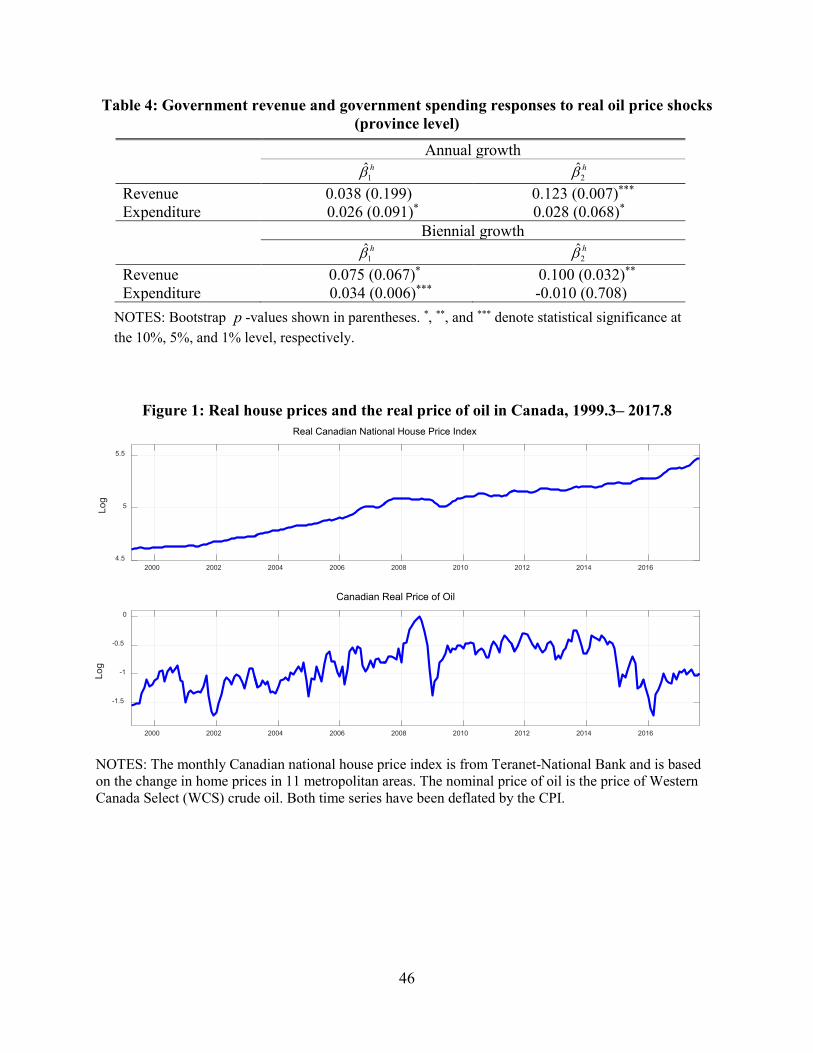
46

2000 2002 2004 2006 2008 2010 2012 2014 20164.5

5

5.5

Log

Real Canadian National House Price Index

2000 2002 2004 2006 2008 2010 2012 2014 2016

-1.5

-1

-0.5

0

Log

Canadian Real Price of Oil

Table 4: Government revenue and government spending responses to real oil price shocks (province level)

Annual growth

1̂hβ 2

ˆ hβ Revenue 0.038 (0.199) 0.123 (0.007)***

Expenditure 0.026 (0.091)* 0.028 (0.068)*

Biennial growth

1̂hβ 2

ˆ hβ Revenue 0.075 (0.067)* 0.100 (0.032)**

Expenditure 0.034 (0.006)*** -0.010 (0.708)

NOTES: Bootstrap p -values shown in parentheses. *, **, and *** denote statistical significance at the 10%, 5%, and 1% level, respectively.

Figure 1: Real house prices and the real price of oil in Canada, 1999.3– 2017.8

NOTES: The monthly Canadian national house price index is from Teranet-National Bank and is based on the change in home prices in 11 metropolitan areas. The nominal price of oil is the price of Western Canada Select (WCS) crude oil. Both time series have been deflated by the CPI.

47

0 5 10 15 20

Months

-0.5

0

0.5

Perc

ent

Canadian real oil price shock

0 5 10 15 20

Months

-0.5

0

0.5

Perc

ent

Employment shock

0 5 10 15 20

Months

-0.5

0

0.5

Perc

ent

Mortgage rate shock

0 5 10 15 20

-0.2

0

0.2

0.4

0.6

Rea

l Hou

se P

rice

(%)

0 5 10 15 20

0

0.1

0.2

0.3

Empl

oym

ent (

%)

0 5 10 15 20

Months

-0.1

-0.05

0

0.05

0.1

0.15

Infla

tion

(%)

0 5 10 15 20

Months

-0.05

0

0.05

0.1

0.15

Mor

tgag

e R

ate

(%)

Figure 2: The effect of selected shocks on real national house prices, 1999.3–2017.8 NOTES: Responses to one-standard-deviation shocks based on the VAR model in section 2.1. The 90% confidence intervals were constructed based on the conditional heteroskedasticity-robust residual block bootstrap of Brüggemann, Jentsch and Trenkler (2016) with block size 24.

Figure 3: The effect of an unexpected increase in the Canadian real price of oil on selected Canadian macroeconomic aggregates, 1999.3–2017.8

NOTES: Responses to one-standard-deviation shock based on the VAR model in section 2.1. The 90% confidence intervals were constructed based on the conditional heteroskedasticity-robust residual block bootstrap of Brüggemann, Jentsch and Trenkler (2016) with block size 24.

48

2000 2002 2004 2006 2008 2010 2012 2014 2016-1

-0.5

0

0.5

1

1.5

2

2.5

3

3.5

4

Calgary

Saskatoon

Vancouver

0 5 10 15 20

-0.2

0

0.2

0.4

0.6

Rea

l Hou

se P

rice

(%)

0 5 10 15 20

0

0.1

0.2

0.3

Empl

oym

ent (

%)

0 5 10 15 20

Months

-0.1

-0.05

0

0.05

0.1

0.15

Infla

tion

(%)

0 5 10 15 20

Months

-0.05

0

0.05

0.1

0.15

Mor

tgag

e R

ate

(%)

Figure 4: The effect of an unexpected increase in the U.S. real price of oil on selected Canadian macroeconomic aggregates, 1999.3–2017.8

NOTES: Responses to one-standard-deviation shock based on the VAR model in section 2.2. The 90% confidence intervals were constructed based on the conditional heteroskedasticity-robust residual block bootstrap of Brüggemann, Jentsch and Trenkler (2016) with block size 24.

Figure 5: Standardized employment shares for selected Canadian cities

49

2 4 6 8

0

0.05

0.1

%

Real house price

2 4 6 8-8

-6

-4

-2

0

2

%

10 -4 Arrear rate

2 4 6 8

0

0.02

0.04

%

Mortgage values

2 4 6 8

0

0.05

0.1%

Personal loans

2 4 6 8

Quarters

0

0.05

0.1

%

Real house price

2 4 6 8

Quarters

-8

-6

-4

-2

0

2

%

10 -4 Arrear rate

2 4 6 8

Quarters

0

0.02

0.04

%

Mortgage values

2 4 6 8

Quarters

0

0.05

0.1

%

Personal loans

2 4 6 8-0.02

0

0.02

0.04

0.06

0.08%

Real house price

2 4 6 80

0.5

1

%

Building permits

2 4 6 80

0.5

1

1.5

%

Housing starts

2 4 6 8

Quarters

-0.02

0

0.02

0.04

0.06

0.08

%

Real house price

2 4 6 8

Quarters

0

0.5

1%

Building permits

2 4 6 8

Quarters

0

0.5

1

1.5

%

Housing starts

Figure 6: Housing market responses to a positive 1% real oil price shock (city level)

1̂hβ

2ˆ hβ

Figure 7: Responses of mortgage markets to a positive 1% real oil price shock

(province level)

1̂hβ

2ˆ hβ

50

2 4 6 8-10

-5

0

5

%10 -3 Unemployment rate

2 4 6 8-0.01

0

0.01

0.02

%

Total employment

2 4 6 8-1

0

1

2

3

4

%

10 -3 Oil sector employment

2 4 6 8

Quarters

-10

-5

0

5

%

10 -3 Unemployment rate

2 4 6 8

Quarters

-0.01

0

0.01

0.02

%

Total employment

2 4 6 8

Quarters

-1

0

1

2

3

4

%

10 -3 Oil sector employment

Figure 8: Labor market responses to a positive 1% real oil price shock (city level)

1̂hβ :

2ˆ hβ :

51

2 4 6 8-1

0

1

2

%10 -3Out-migration

2 4 6 8-1

0

1

2

%

10 -3 In-migration

2 4 6 8-1

0

1

2

%

10 -3 Net-migration

2 4 6 8

Quarters

-1

0

1

2

%

10 -3Out-migration

2 4 6 8

Quarters

-1

0

1

2%

10 -3 In-migration

2 4 6 8

Quarters

-1

0

1

2

%

10 -3 Net-migration

Not-for-Publication Appendix:

Figure A1: Net migration responses to a positive 1% real oil price shock (province level) NOTES: Based on quarterly estimates of interprovincial in- and out-migration from Canada Revenue Agency (CRA) tax data showing changes in permanent residence.

Figure A2: Interprovincial net migration and the real oil price of oil Notes: See Figure A1.

52

Figure A3: Response of aircraft movements to a positive 1% real oil price shock

NOTES: Total number of aircraft movements in city airports with Nav Canada towers.

1 2 3 4 5 6 7 8

Quarters

-0.1

-0.08

-0.06

-0.04

-0.02

0

0.02

0.04

%1: Aircraft movements

1 2 3 4 5 6 7 8

Quarters

-0.1

-0.08

-0.06

-0.04

-0.02

0

0.02

0.04

%

2: Aircraft movements