To be published by SPIE in: Remote Sensing of the Atmosphere, Ocean, Environment, and Space, Proc. SPIE, 4896, 2002.

- 1 -

The quality of data from the National Science Foundation's UV Monitoring Network for Polar Regions

Germar Bernhard*, Charles R. Booth**, James C. Ehramjian***

Biospherical Instruments Inc., San Diego

ABSTRACT The U.S. National Science Foundation’s network for monitoring UV radiation in polar regions is now in its 15th year of operation. During this period, the deployed SUV-100 spectroradiometers have repeatedly been modified, and data processing methods have been changed. These modifications have continuously improved the quality of published data, but have also introduced step-changes into the data set. For example, a change of the wavelength calibration method in 1997 has improved the wavelength accuracy to ±0.04 nm (±1σ), but also lead to a step of 2-4% in published biological dose rates. In order to best assess long-term changes in UV at network locations, it is desirable to remove these steps and to homogenize the data set. This publication discusses possible ways to accomplish these objectives, with special emphasis on absolute calibration, wavelength accuracy, and the cosine error. To date, published data are not corrected for the instruments’ cosine errors. Such corrections are not straightforward, as older data are affected by an azimuth asymmetry of the irradiance collector, which was not constant over the years. A new method to correct the errors for both clear and cloudy sky conditions was developed, and is described here. Results indicate that dose rates published prior to the year 2000 are low by 2-5%, and exhibit a variation with the Sun’s azimuth angle. By modifying the instruments’ irradiance collectors in 2000, the azimuth asymmetry was virtually eliminated, however, the modification also lead to a step-change of about 3% in published data. The ability of the new correction algorithm to remove this step is demonstrated. Uncertainties in biologically weighted dose rates caused by the cosine error can be reduced with the correction procedure to ±2%. We are planning to reprocess the entire NSF data set with the new algorithms to improve both accuracy and homogeneity. Keywords: Solar ultraviolet radiation, Antarctica, QA/QC, cosine correction

1. INTRODUCTION Any network of research instruments operating in harsh environments over more than 10 years is likely to be affected by changes in instrumentation, operation, and data processing procedures. Some modifications may be imposed from outside (e.g. relocation of instruments), and some are implemented from experience gained over the years in working with the instruments and their data. These modifications can affect published data and conclusions drawn from their analysis. For example, improving instrumentation can lead to more accurate data products but potentially introduce artificial trends into time series that are constructed from older and newer data. One objective of this paper is to describe modifications to deployed SUV-100 spectroradiometers and data processing algorithms of the U.S. National Science Foundation’s Office of Polar Program's UV monitoring network, operated by Biospherical Instruments Inc. A second goal is to present new procedures that will further improve the accuracy of published data. The most significant modifications are related to absolute calibration (Section 2), wavelength calibration (Section 3), and the cosine error1-6 (Section 4). The main focus is on the cosine error as changes in absolute and wavelength calibration are well documented in our Operations Reports7, available on the web at www.biospherical.com/NSF. As of this writing, published data are not corrected for the cosine error. Section 4 proposes a new algorithm to correct the effect of this error on solar data. This algorithm is considerably more elaborate than similar procedures published elsewhere1-6 as the cosine error of the SUV-100 instruments prior to 2000 was

* bernhard@biospherical.com; phone 1 619 686-1888; fax 1 619 686-1887; http://www.biospherical.com; Biospherical Instruments Inc., 5340 Riley Street, San Diego, CA 92110-2621, USA; ** booth@biospherical.com; *** jime@biospherical.com

- 2 -

dependent on wavelength and the solar azimuth angle. In most cosine correction algorithms, the cosine error is only a function of zenith angle. In 2000, the collectors of all instruments were modified to remove their azimuth and wavelength dependency. This introduced a step-change, which can be removed by the proposed correction procedure. The effect of the cosine error on solar data is generally dependent on whether the Sun is visible or not. The proposed algorithm therefore also includes the treatment of clouds. Table 1 gives an overview of major events affecting NSF network data. In addition, there were several periods when the accuracy of data was reduced due to instrumental problems or calibration drifts. Those events are documented in detail in Operations Reports7 and will not be discussed here. In 1996 and 1997, the Operating System of all system control computers was changed from DOS to a Windows NT. With introduction of the new Windows NT software, the scanning frequency was increased to four solar spectra per hour. The higher sampling rate required shorter integration times. Data from 1997 onward have therefore a slightly reduced detection limit. We are planning to cosine-correct the whole NSF data set and also apply the new wavelength calibration described in Section 3 to all data. This will eventually lead to a new data version.

Table 1: Overview of major instrumentation and data processing changes

Activity Site McMurdo Palmer South Pole Ushuaia San Diego Barrow Initial Installation Mar 1988 May 1988 Feb 1988 Nov 1992 Nov 1992 Dec 1990 Instrument Relocation Mar 1993 1991, 1997 Software / OS upgrade 12/12/96 1/15/97 2/2/97 2/5/97 8/6/96 6/10/96 Change wavelength correction 1/18/97 4/19/97 2/1/97 4/2/97 9/9/97 10/26/97 Upgrade cosine collector 2/6/00 3/19/00 1/26/00 6/28/00 9/9/00 Dec 2000 Cosine corrected data Planned for 2003

2. ABSOLUTE CALIBRATION The radiometric calibration of the instruments is performed with 200-Watt Standards of Spectral Irradiance, which are procured from Optronic Laboratories Inc (OLI). The lamps are calibrated by OLI relative to standards provided by the National Institute of Standard and Technology (NIST). At least two OLI standards are available at every site and are used for bi-weekly calibrations. The standards are compared once a year to a “traveling” standard, the calibration of which is particularly well maintained and documented. This standard is used at all instrument locations to ensure that the same scale of irradiance is maintained at all sites. Whenever a site standard is found to have drifted by more than 2% it is either recalibrated or replaced. In addition, our OLI standards are regularly compared to standards provided by NOAA’s Central UV Calibration Facility (CUCF). Changes in responsivity of the SUV-100 spectroradiometers are corrected when drifts exceed 2%, utilizing data from the bi-weekly calibrations and automatic daily measurements of a 45-Watt lamp, which is an integral part of the instruments’ fore-optics. All changes in calibration standards and calibration equipment, as well as adjustments for drifts in instrument responsivity and operator errors are thoroughly documented in Operations Reports7. We currently have no evidence of any long-term drift of our calibration scale. However, NIST has recently adjust their irradiance scale, which may have an impact on future data of the NSF network. Calibration procedures have been refined over time with the objective of reducing uncertainties. In the early years of the network, power supplies used with standard lamps were manually set to a target current of 6.5 A. The current was measured directly with digital multimeters (DMM). The accuracy of the DMMs were annually verified with a traveling DMM and precision shunt. The accuracy of the current measurement was improved in 1991 when shunts were installed in series with the lamps at all sites, and the lamp current was determined by measuring the voltage drop across the shunt. In order to reduce the likelihood of setting the lamp current incorrectly, computer controlled power supplies and voltmeters were installed over the period from 1992 through 1993. Prior to 1992, 200-Watt calibration lamps were held in place with wire leads that were only connected prior to each calibration scan according to instructions from OLI. The lamps were calibrated by OLI with the filament in vertical orientation, but used in the field with the filament oriented horizontally. Experiments performed in 1992 indicated that this change in orientation leads to an irradiance change of 1.4±0.5%. In response to this problem, the lamp mounting

- 3 -

was redesigned providing a separate holder for every lamp. The lamps were effectively permanently connected to these holders, which could be removed from the calibration stand without the risk of bending the wire leads. The improved mounting lead to reproducible positioning of the lamps relative to the collector of the SUV-100. We also directed OLI to calibrate the lamps in the same orientation as we used them in the field. The implementation of the new lamps started in 1993. Data prior to this year may have a 1-2% systematic error related to the lamps’ sensitivity to orientation. We intend to confirm the magnitude of this error and correct affected data. Also in the early years of network operation, instruments were not completely temperature stabilized, which resulted in responsivity drifts. These drifts could not be corrected completely. In particular, Ushuaia data from 1989 and 1990 showed extensive periods of instability related to temperature variations. The periods affected are not part of the published data set and are only available to researchers on specific request. We are planning to revisit the calibration records of these early network data with the goal of uncovering systematic errors, should they exist, and to apply appropriate corrections.

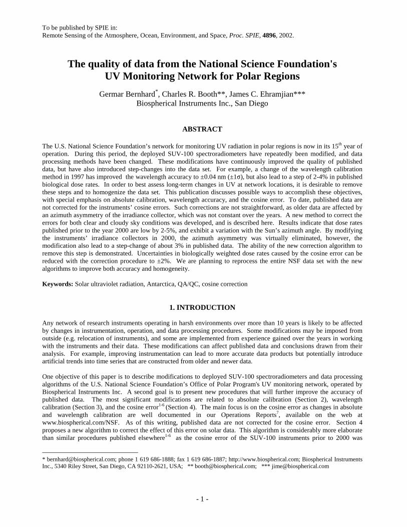
3. WAVELENGTH CALIBRATION Until 1997, the wavelength calibration of the systems was based on daily automatic scans of a mercury lamp integrated into the instruments’ fore optics. By comparing the locations of spectral lines in measured spectra of this lamp with the actual mercury line positions, the wavelength mapping of the monochromator was established and applied to solar spectra. Analysis revealed that solar spectra calibrated with this method exhibit a wavelength shift of about 0.1 nm at 300 nm. This shift can be attributed to the difference in the illumination of the monochromator by the mercury lamp and by the irradiance collector. Data from Volume 7 onward (see Table 1 for dates) are calibrated with a different method, which lead to a significant improvement in wavelength accuracy. The new method utilizes the Fraunhofer structure in solar spectra. This structure is also very marked in spectra of solar irradiance measured with the SUV-100 radiometers. The method applied here is based on the implementation by Slaper et al.8-10. The reference solar spectrum is based on a high-resolution (< 0.001 nm) extraterrestrial spectrum measured by the Fourier-Transform Spectroradiometer (FTS) at the National Solar Observatory (NSO) located at Kitt Peak, Arizona11. The original spectrum was slightly modified to account for an erroneous peak in the Kitt Peak spectrum in the 320-330 nm range10. The wavelength accuracy of this spectrum has been shown to be better than 0.003 nm. The method has been successfully used during several intercomparison campaigns8-10,12,13. The wavelength accuracy of solar SUV-100 spectra corrected with the new method is ±0.04 nm (±1σ). This can be concluded from results of two independent Fraunhofer structure correction algorithms8,14. A detailed description of the implementation and its uncertainty evaluation can be found in Operations Reports7 of the NSF UV network. Small errors in wavelength calibration have a significant effect on measured biologically relevant dose rates due to the strong increase of the solar spectrum in the UV-B. In order to determine the effect of change in the wavelength calibration method, one year of data from San Diego was corrected with both the “old” mercury lamp method and the “new” Fraunhofer line correlation method (Figure 1). At a solar zenith angle (SZA) of 50°, values corrected with the old method are lower by 2% for erythemal15 and 4% for DNA damaging16 irradiance. For DNA irradiance, the difference is nearly independent of SZA, whereas the difference in erythemal values appears to be smaller at larger SZA. For the integral of measurements between 303.0-307.7 nm, the difference is about 4% at 30° SZA. At 75° SZA, the difference increases to 6.5% and then diminishes again towards larger SZAs. The reason for this change with SZA is the different shape of the solar spectrum at different solar elevations. The SZA dependence is also somewhat affected by total column ozone. Theoretical evaluations show that this dependence is not large for erythemal and DNA irradiances17. Results depicted in Figure 1 can therefore also be applied to data from high-latitude sites.

- 4 -

In conclusion, biological dose rates published prior to 1997 appear to be low by approximately 2-4%, almost independent of solar zenith angles. Systematic errors in short-wave UV-B irradiances, like the 303-307.7 nm integral, are somewhat larger, and SZA-dependent. If newer data are compared with historic data, this step-change should be taken into consideration.

0.9

0.92

0.94

0.96

0.98

1

1.02

1.04

0 20 40 60 80

Solar Zenith Angle (Degrees)

Rat

io O

ld /

New

cor

rect

ion

Integral 303.0 - 307.7 nm

DNA damaging radiation (Setlow)

Erythema (CIE)

Figure 1. Effect of wavelength correction method on spectral integrals. Small symbols show the ratios of data that were corrected with the historic mercury lamp based method, to data corrected with the new Fraunhofer method. Three different data sets are depicted, including the 303.0-307.7 nm integral, DNA damaging radiation and erythemal irradiance. Large symbols show theoretical results17.

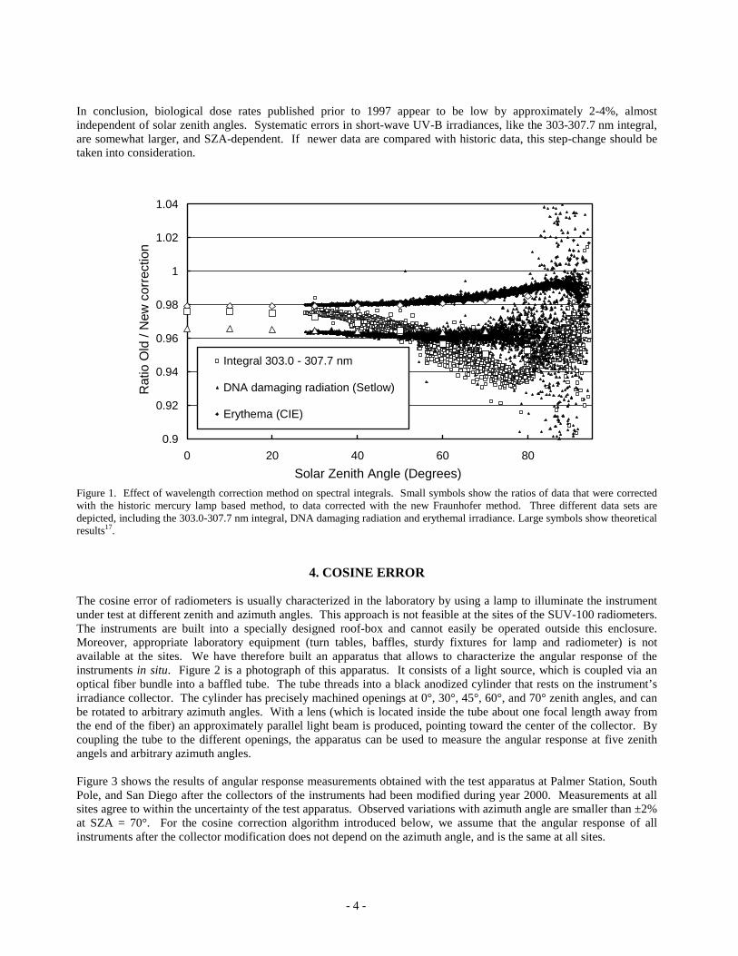
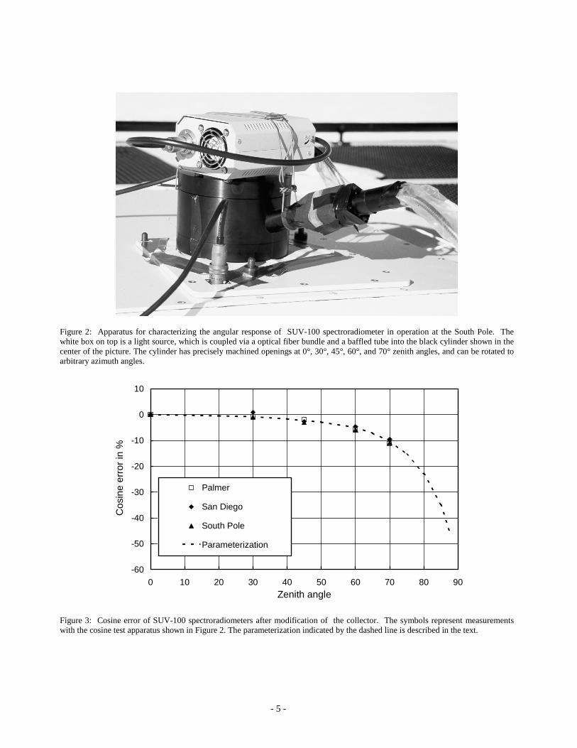
4. COSINE ERROR The cosine error of radiometers is usually characterized in the laboratory by using a lamp to illuminate the instrument under test at different zenith and azimuth angles. This approach is not feasible at the sites of the SUV-100 radiometers. The instruments are built into a specially designed roof-box and cannot easily be operated outside this enclosure. Moreover, appropriate laboratory equipment (turn tables, baffles, sturdy fixtures for lamp and radiometer) is not available at the sites. We have therefore built an apparatus that allows to characterize the angular response of the instruments in situ. Figure 2 is a photograph of this apparatus. It consists of a light source, which is coupled via an optical fiber bundle into a baffled tube. The tube threads into a black anodized cylinder that rests on the instrument’s irradiance collector. The cylinder has precisely machined openings at 0°, 30°, 45°, 60°, and 70° zenith angles, and can be rotated to arbitrary azimuth angles. With a lens (which is located inside the tube about one focal length away from the end of the fiber) an approximately parallel light beam is produced, pointing toward the center of the collector. By coupling the tube to the different openings, the apparatus can be used to measure the angular response at five zenith angels and arbitrary azimuth angles. Figure 3 shows the results of angular response measurements obtained with the test apparatus at Palmer Station, South Pole, and San Diego after the collectors of the instruments had been modified during year 2000. Measurements at all sites agree to within the uncertainty of the test apparatus. Observed variations with azimuth angle are smaller than ±2% at SZA = 70°. For the cosine correction algorithm introduced below, we assume that the angular response of all instruments after the collector modification does not depend on the azimuth angle, and is the same at all sites.

- 5 -

Figure 2: Apparatus for characterizing the angular response of SUV-100 spectroradiometer in operation at the South Pole. The white box on top is a light source, which is coupled via a optical fiber bundle and a baffled tube into the black cylinder shown in the center of the picture. The cylinder has precisely machined openings at 0°, 30°, 45°, 60°, and 70° zenith angles, and can be rotated to arbitrary azimuth angles.

-60

-50

-40

-30

-20

-10

0

10

0 10 20 30 40 50 60 70 80 90Zenith angle

Cos

ine

erro

r in

%

Palmer

San Diego

South Pole

Parameterization

Figure 3: Cosine error of SUV-100 spectroradiometers after modification of the collector. The symbols represent measurements with the cosine test apparatus shown in Figure 2. The parameterization indicated by the dashed line is described in the text.

- 6 -

The test apparatus is limited to measurement of the cosine response for zenith angles up to 70°, as mounting of the illumination tube at larger angles is not possible due to mechanical reasons. Cosine errors at larger SZA were determined by using the Sun as the light source. For this method, we took advantage of the instrument’s ability to measure spectral solar irradiance to up to 600 nm, where global irradiance is dominated by the direct solar beam. For example at the South Pole, at SZA = 80°, the contribution of the direct beam to global irradiance is about 83% at 600 nm, compared to 7% at 330 nm. Measurements at long wavelengths are much more sensitive to the cosine error than measurements at short wavelengths. The cosine error for SZAs larger than 70° was estimated from the difference of clear-sky irradiance and results of a radiative transfer model (see below) at 600 nm. Note that such a comparison may be affected by aerosol. Although small amounts of aerosol only lead to a small reduction of global irradiance, aerosol can cause an appreciable change in the ratio of direct to global irradiance. The extrapolation of the cosine error to large SZAs was performed with data from the South Pole where the influence of aerosols is negligible18. The dashed line in Figure 3 shows the final parameterization of the cosine error based on measurements with the test apparatus and the extrapolation with solar measurements at the South Pole. 4.1. Cosine correction for clear sky conditions The effect of the cosine error on solar measurements is described in several publications1-6. The ratio fG of global irradiance measurements that are affected by this error and the “true” global irradiance can be expressed by the following equation2:

)),(1()(),(),(),( λθ−λ+λθλθ=λθ RfRff DBG ,

where θ is solar zenith angle (SZA), λ is wavelength, ),( λθBf is the cosine error, defined here as the ratio of measured to “true” direct irradiance from the

Sun’s direct beam on a horizontal surface, Ω is solid angle, )(λDf is the diffuse cosine error, defined here as the error in measuring isotropic radiance originating

from the upper hemisphere: )(λDf = ΩθΩθλθ ∫∫ ππddfB )2()2(

)cos()cos(),( , and

),( λθR is the ratio of direct irradiance ),( λθB and Global Irradiance ),( λθG : ),(),(),( λθλθ=λθ GBR .

Measurements with the test apparatus after the collector modification did not indicate any significant dependence of the collectors’ angular response on wavelength. We therefore approximate ),( λθBf with the parameterized function

shown in Figure 3. The diffuse error )(λDf calculated from this function is 0.954. For clear sky conditions, ),( λθR is

calculated with the radiative transfer model UVSPEC/libRadtran19. In addition to θ and λ , ),( λθR depends on all

parameters affecting the transfer of radiation through the atmosphere. Most important are ground albedo and aerosol optical depth. For operational data processing it is not practical to adjust these parameters for every spectrum to be corrected. We therefore implement climatological mean values. Deviations from these values contribute to the uncertainty of the correction method. The most prominent factor modifying ),( λθR are clouds. The influence of clouds

is calculated for every spectrum with a method introduced in Section 4.2. As mentioned previously, the cosine error ),( λθBf of all SUV-100 instruments was dependent on azimuth angle and

wavelength prior to the year 2000. This dependency can be approximated by the following equation:

)),(sin(),(),(),,( λθ+ϕλθ+λθ=ϕλθ cbaf B ,

where ϕ is solar azimuth angle, and a, b and c are empirically derived coefficients dependent on θ and λ .

(1)

(2)

- 7 -

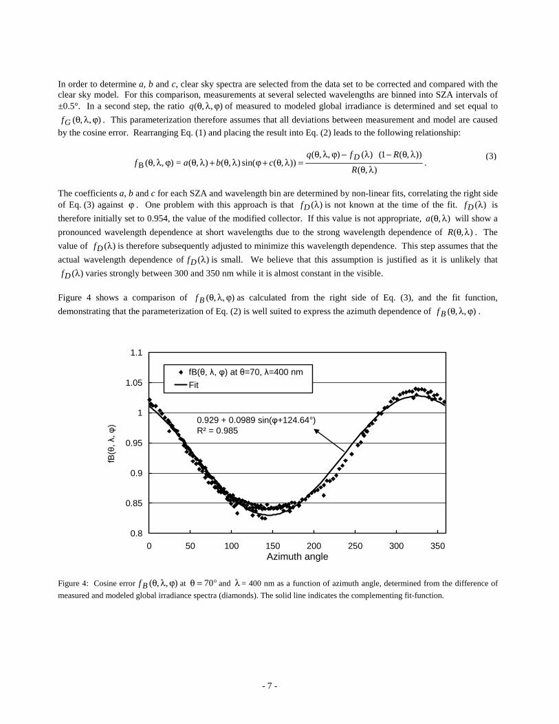
In order to determine a, b and c, clear sky spectra are selected from the data set to be corrected and compared with the clear sky model. For this comparison, measurements at several selected wavelengths are binned into SZA intervals of ±0.5°. In a second step, the ratio ),,( ϕλθq of measured to modeled global irradiance is determined and set equal to

),,( ϕλθGf . This parameterization therefore assumes that all deviations between measurement and model are caused

by the cosine error. Rearranging Eq. (1) and placing the result into Eq. (2) leads to the following relationship:

),(

)),(1()(),,()),(sin(),(),(=),,( B λθ

λθ−λ−ϕλθ=λθ+ϕλθ+λθϕλθ

R

Rfqcbaf

D.

The coefficients a, b and c for each SZA and wavelength bin are determined by non-linear fits, correlating the right side of Eq. (3) against ϕ . One problem with this approach is that )(λDf is not known at the time of the fit. )(λDf is

therefore initially set to 0.954, the value of the modified collector. If this value is not appropriate, ),( λθa will show a

pronounced wavelength dependence at short wavelengths due to the strong wavelength dependence of ),( λθR . The

value of )(λDf is therefore subsequently adjusted to minimize this wavelength dependence. This step assumes that the

actual wavelength dependence of )(λDf is small. We believe that this assumption is justified as it is unlikely that

)(λDf varies strongly between 300 and 350 nm while it is almost constant in the visible.

Figure 4 shows a comparison of ),,( ϕλθBf as calculated from the right side of Eq. (3), and the fit function,

demonstrating that the parameterization of Eq. (2) is well suited to express the azimuth dependence of ),,( ϕλθBf .

0.8

0.85

0.9

0.95

1

1.05

1.1

0 50 100 150 200 250 300 350Azimuth angle

fB(θ

, λ, φ

)

fB(θ, λ, φ) at θ=70, λ=400 nm

Fit

0.929 + 0.0989 sin(φ+124.64°) R² = 0.985

Figure 4: Cosine error ),,( ϕλθBf at °=θ 70 and λ = 400 nm as a function of azimuth angle, determined from the difference of

measured and modeled global irradiance spectra (diamonds). The solid line indicates the complementing fit-function.

(3)

- 8 -

The coefficients ),,( λθa ),,( λθb and ),( λθc are smooth functions of ,θ and can therefore be approximated by

polynomials:

2210

43

2210

43

2210

)()()(),(

)()()()(),(

)()()()(),(

θλ+θλ+λ=λθθλ+θλ+θλ+λ=λθ

θλ+θλ+θλ+λ=λθ

rrrc

qqqqb

ppppa

The coefficients ),(λip ),(λiq and )(λir with 3,2,1,0=i are determined by non-linear fits. As shown below, there is

no evidence that ),( λθa depends on wavelength. We therefore select a representative set of coefficients )(λip and

apply this set to all wavelengths. In contrast, )(λiq and )(λir are complicated functions of wavelength, which cannot

be approximated by simple analytical functions. The coefficients are therefore calculated at discrete wavelengths and interpolated to all wavelengths of the solar spectrum to be corrected. The wavelength dependence of )(λiq and )(λir is caused by anomalies in the efficiency of the monochromator’s

gratings (Wood’s anomalies20), and the sensitivity of the location of these anomalies to the angular distribution of light entering the monochromator. This distribution is dependent on the azimuthal position of the light source (either Sun or cosine test apparatus) illuminating the instrument’s collector. The collector of the SUV-100 spectroradiometers is a diffuser made of Teflon, which has trapezoidally shaped walls7. These walls are brighter at the side of the illumination. The change in geometry as a function of azimuth angle leads to a change in the illumination of the monochromator’s gratings. The diffuser modification consisted of an aperture behind the diffuser which prevents radiation originating from the trapezoidally shaped walls from entering the monochromator. With the aperture installed, the azimuth artifacts in solar data are virtually eliminated. Flat diffusers typically lead to a negative cosine error at large incidence angles4, partly because the reflection of radiation off the diffuser increases with increasing incidence angle. In order to compensate for the reflection losses, contemporary diffuser designs have raised walls21, or use spherical4 or trapezoidally shaped diffusers, such as in our case. By installing the aperture, it can be expected that the average cosine error of the instrument increases. Results shown below indicate that this is in indeed the case. However, the effect is small (about 1.5% increase in )(λDf ) and

is outweighed by the benefit of removing the azimuth asymmetry. One caveat of the approach using a measurement-model comparison for the determination of the ),,( ϕλθBf , is that

the measurement is forced to agree with model values, which are not necessarily correct. This issue is less problematic for coefficients b and c, which express the amplitude and phase of the azimuth dependence, respectively. Real atmospheric processes do not vary sinusoidally with the azimuth. It can therefore be assumed that variations of this kind are an artifact of the measurement (otherwise solar measurements with the modified collector would show similar signatures, which is not the case). In contrast, coefficient ),( λθa corrects for general level-differences between

measurement and model, which may be caused both by inappropriate model input parameters or systematic errors in the measurement. For example, if albedo is set too high in the model, modeled values will be too high and the ratio measurement to model will be too low. The correction algorithm will attribute this to the cosine error of the instrument, leading to an over-correction of the measurements. The determination of ),( λθa therefore cannot be based on models

alone, but requires independent verification. We have therefore compared the model-based estimate of ),,( ϕλθBf with angular response measurements obtained with the test apparatus before the collector modification.

Figure 5 shows ),,( ϕλθBf as a function of wavelength at °=θ 70 for three azimuth angles, determined from both in

situ measurements and the parameterization based on Eqs. (2) and (4). The spike in the response at 505 nm is caused by the grating anomaly, and is well reproduced by both in situ measurement and the parameterization. At ,0°=ϕ the

agreement of both data sets is almost ideal. At °=ϕ 180 and 270°, there is a difference of about 2%, which is still

within the expected uncertainties of both measurements and parameterization. The good agreement indicates that the model-based approach is feasible for correcting the instrument’s cosine error. Below 330 nm, the in situ measurement becomes unreliable due to low signal levels. Below this wavelength, the parameterization is also problematic, partly

(4)

- 9 -

because of the small values of ),( λθR and partly because of the increasing influence of ozone absorption. Due to these

constraints, we apply )nm 330,(θa at shorter wavelengths also. This is justified as ),,( ϕλθGf is dominated by

)(λDf rather than ),,( ϕλθBf at short wavelengths.

We calculated the mean cosine error at °=θ 70 , by averaging the results of the in situ measurements over all azimuth angles (broken line with triangles in Figure 5). The error is almost independent of wavelength and is on average –6.5%. This confirms the previous assumption that ),( λθa is independent of λ . The average cosine error at 70° of the

parameterization is –6.1%, independent of wavelength by construction. The cosine correction of a clear sky solar spectrum that was measured prior to the diffuser upgrade is finally performed by dividing the measured global spectral irradiance with ),( λθGf , which in turn is calculated for each wavelength of

the spectrum using Eq. (1) and the parameterized cosine error ),,( ϕλθBf .

0.8

0.85

0.9

0.95

1

1.05

1.1

1.15

1.2

300 350 400 450 500 550 600 650

Wavelength in nm

fB(θ

, λ, φ

)

Measurement with test apparatus

Parameterization

Azimuthal average test apparatus

Azimuthal average parameterization

φ=270°

φ=180°

φ=0°

Figure 5: Cosine error ),,( ϕλθBf at °=θ 70 as a function of wavelength for the azimuth angles 0°, 180°, and 270°. Thin lines

indicate results obtained from measurements with the test apparatus during the site visit at the South Pole in January 2000. Thick lines are based on the parameterization using the set of coefficients ),(λip ),(λiq and )(λir . The broken lines give the

azimuthally averaged cosine errors based on measurement and parameterization. 4.2. Cosine correction for cloudy conditions Clouds lead to a spatial redistribution of radiation. The involved processes are too complex to be considered in an exact manner, and simplifications are therefore required. For the correction algorithm we assume that clouds are homogeneous and stratiform, and can be parameterized by a lower and upper boundary, and cloud optical depth τ. In brief, the algorithm estimates τ from the comparison of measured global irradiance under clouds with clear sky model values. In a second step, the ratio of direct and global irradiance ),( λθR is calculated with the radiative transfer model

using the previously-established cloud optical depth as an additional input parameter. The procedure is an extension of a method recently proposed22. For large cloud optical depths, ),( λθR becomes 0, and Eq. (1) simplifies to

)(),( λ=λθ DG ff . The error ),( λθGf becomes therefore independent of τ. There is no evidence that the diffuse

- 10 -

cosine error )(λDf of SUV-100 spectroradiometers is wavelength dependent. Spectra measured under optically thick

clouds are corrected by scaling measured global irradiance with the constant factor of .1 Df The algorithm steps are

outlined as follows:

1- Calculate a suite of global and direct irradiance spectra with the radiative transfer model for a wide range of SZAs θ , and cloud optical depths τ.

2- Extract spectral global irradiance at a wavelength in the visible (typically 550 nm) from all modeled spectra, which leads to a two dimensional matrix of global irradiance ),,( τλθG at 550 nm as a function of SZA and τ .

The matrix is denoted ),( τθM in the following.

3- Determine the direct to global ratio ),,( τλθR at 550 nm for all model spectra.

4- Calculate the error function ),,( τλθGf at 550 nm for each model spectra, using ),,( τλθR from Step 3, and

the parameterization of ),,( ϕλθBf introduced in Section 4.1. Note that ),,( τλθGf is also dependent on the

azimuth angle ϕ of the measured spectrum to be corrected.

5- Multiply the matrix ),( τθM with ),nm 550,( τθGf . This leads to a modified matrix ),(' τθM , which now

represents cosine-error affected global irradiance ),,( τλθG model values at 550 nm as a function of SZA and τ

. 6- Determine the ratio )(θs of cosine-corrected clear-sky measurements and clear sky model values. This ratio is

required to take into account any difference between corrected measured spectra and modeled spectra under clear skies, which would otherwise be interpreted as cloud effect in the steps below.

7- Estimate cloud optical depth τ. This is done by comparing the measured cloud attenuation ),nm, 550,( τθA defined as

)()0,nm 550,()0,nm 550,(

)nm, 550,( )nm, 550,(

θ⋅θ⋅θτθ

=τθsfG

GA

G

M

with the simulated matrix ),(' τθM . In Eq. (5), )nm, 550,( τθMG is the measured, uncorrected, global

irradiance at 550 nm under a cloud with optical depth τ. The denominator )()0,nm 550,()0,nm 550,( θ⋅θ⋅θ sfG G represents simulated, uncorrected clear sky irradiance at 550 nm. Under

broken-cloud conditions, )nm, 550,( τθA can be larger than one. In this case, τ is set to 0.

8- Determine the direct to global ratio ),,( τλθR for all wavelengths of the spectra to be corrected. ),,( τλθR is

calculated by interpolating the suite of model spectra from Step 1 to the zenith angle of the measured spectrum, and cloud optical depth that was estimated in Step 7.

9- Calculate ),,( τλθGf , using Eq. (1) and ),,( τλθR from the previous step.

10- Correct the measured spectrum by scaling it with ),,(1 τλθGf .

The procedure outlined above estimates cloud optical depth from the attenuation of global irradiance at 550 nm. We use a wavelength in the visible rather than in the UV, despite the fact that UV radiation is the main focus of our project. The reason is that visible radiation is more attenuated by clouds than UV radiation. This phenomenon is due to the wavelength dependence of Rayleigh-scattering: radiation that is reflected upward by clouds is partly backscattered by air molecules situated above the cloud. Backscatter is more likely at shorter wavelength, and photons with shorter wavelengths therefore have a greater probability of reaching the top of the cloud a second time, and to traverse the cloud in a second attempt23. For similar reasons, Rayleigh-scattering occurring between ground and cloud ceiling mitigates cloud attenuation more effectively at shorter wavelengths24. Multiple reflections between snow covered ground and cloud ceiling lead to a further modification of the spectral influence of clouds. Because of these effects, global irradiance in the UV is not a sensitive indicator for cloud optical depth. This is particularly true for places with high albedo. For example, model calculations for °=θ 75 at the South Pole (UV albedo = 97%25) indicate that a cloud with τ=0.3 leads to a 3.8% attenuation of global irradiance at 350 nm but 10% at 550 nm. Despite the small effect on

(5)

- 11 -

global irradiance, clouds lead to pronounced reduction of the direct to global ratio: ),nm 350,75( τ°R is 0.26 for τ=0 but

only 0.085 for τ=0.3. The relative insensitivity of global irradiance to clouds combined with the large sensitivity of ),,( τλθR to clouds is the most important source of uncertainty of the cosine correction algorithm under thin clouds

(i.e. τ<0.3). However, those clouds are relatively rare. For example, only 1901 (11%) of the 17540 spectra measured at the South Pole between January 1999 and January 2000 were found to have an cloud optical depth between 0 and 0.3. 10291 (59%) spectra were rated as clear-sky and 5348 (30%) as cloudy sky. In 89% of the cases, either the clear sky correction or “thick cloud” correction (i.e. scaling with factor Df1 ) was performed. Both cases have lower

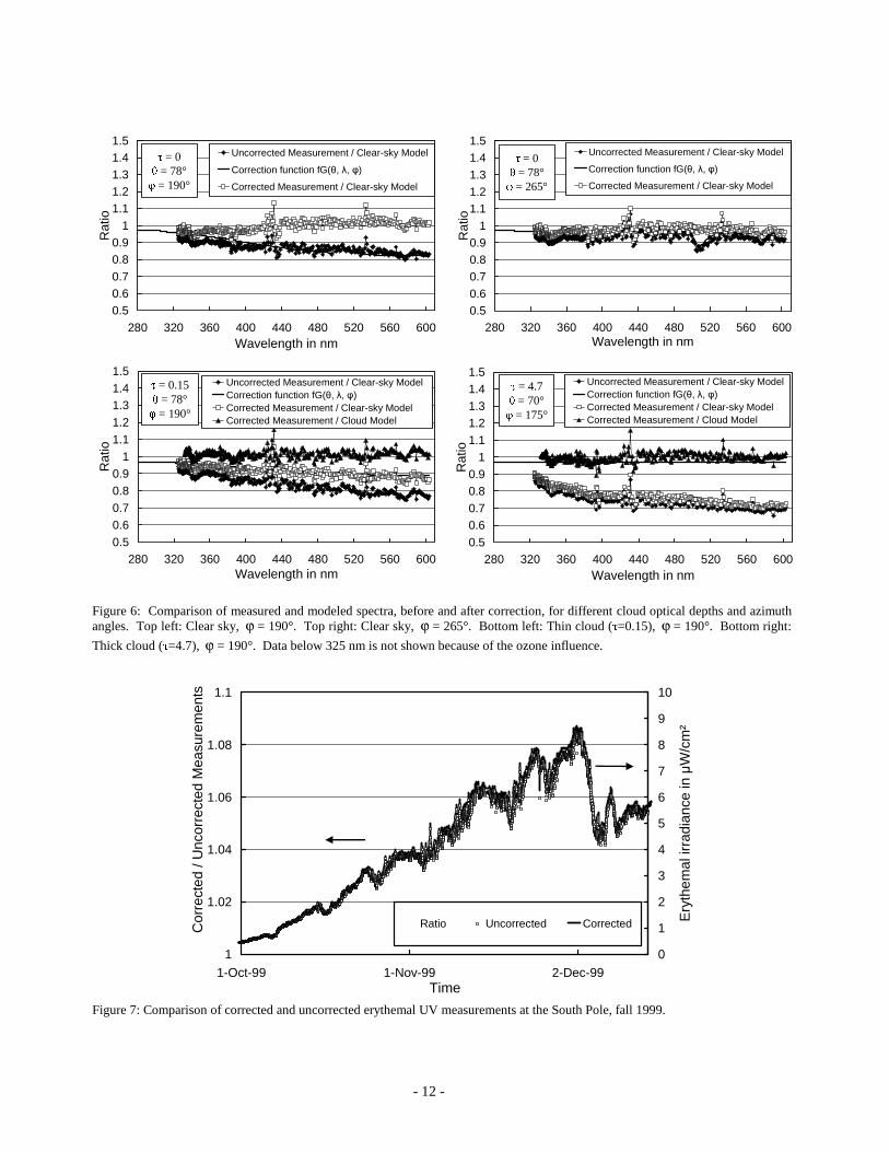
uncertainty. 4.3. Results of cosine correction algorithm Figure 6 shows the result of the new cosine correction algorithm for four spectra measured during clear sky (upper panels), during a thin cloud with τ=0.15 (bottom left panel), and a thick cloud with τ=4.7 (bottom right panel). All spectra are from the Volume 9 South Pole data set and were recorded in 1999 before the collector modification. All panels of Figure 6 show (i) the ratio of uncorrected spectra to the clear sky model; (ii) ),,( τλθGf ; and (iii) the ratio of

corrected spectra to clear sky model. The two bottom panels additionally include (iv) the ratio of corrected spectra to the cloud model. At the longest wavelengths, the uncorrected clear sky spectra deviate from the model by up to 20%. Deviations for wavelengths in the UV are typically smaller than 10%. The corrected spectra agree to within 5% with the model. Note that the monochromator anomaly, which is apparent in the top right panel at 505 nm, is removed by the correction. In the case of the thin cloud, the corrected measurement is less than the clear sky spectra, as one would expect. The ratio of the corrected spectra to the cloud model is close to one for all wavelengths. The agreement at 550 nm is self-evident, as this was the wavelength used for the determination of the cloud optical depth. The fact that there is good agreement at the other wavelengths also gives confidence in the accuracy of the correction algorithm. In the case of the thick cloud, the correction consists of multiplying the measured spectral irradiance by .97.011 =Df In this case

also, the corrected spectra and the cloud model are in good agreement at all wavelengths. The comparison of the ratios (iii) and (iv) confirms that clouds attenuate less in the UV, for reasons explained in Section 4.2. In order to estimate the effect of the cosine correction on biologically relevant dose rates, all spectra from the Volume 9 South Pole data set were cosine-corrected and compared with the uncorrected data set. Figure 7 shows the ratio of corrected to uncorrected erythemal irradiance. For clear sky spectra, the correction varies between 2.2% and 5.5%; for “thick clouds” it is 3.1%. Note that erythemal irradiance changes from 8.5 µW/cm² on 12/2/99 to 4.5 µW/cm² on 12/5/99. This rapid step-change of almost 50% is caused by the dissipation of the “ozone hole”, and is more than 10-times larger than the cosine correction. The cosine correction for DNA damaging radiation varies between 2.4% and 4.9%. Similar correction factors can also be expected for data based on other action spectra as the cosine correction factors do not vary significantly over the spectral region where most biological damage occurs. The correction becomes however large as wavelength increases because of the larger contribution of radiation from the direct solar beam. For example at °=θ 75 and 450 nm, the correction factors vary between 0.97 and 1.17, dependent on the azimuth angle. In order to investigate the effect of the collector modification in January 2000, we also corrected Volume 10 data from 2000 (measured after the collector change), and compared the results with the cosine-corrected Volume 9 data set from 1999. The correction of Volume 10 data is based on a simplified algorithm that is based on Eq. (1) and the parameterized cosine error shown in Figure 3. As the collector change removed the dependence of the cosine error on ϕ , the procedure does not require the azimuth angle. The diffuse correction factor Df1 is 1.049. The treatment of

clouds was the same for data of both seasons. For erythemal irradiance and clear sky conditions, the correction of Volume 10 data varies between 6% and 7% for SZAs between 66° and 82°. For DNA damaging radiation the correction varies between 5.5% and 6.6%. The correction factor for “thick clouds” is 5%, regardless of the action spectrum.

- 12 -

0.50.60.70.80.9

11.11.21.31.41.5

280 320 360 400 440 480 520 560 600Wavelength in nm

Rat

io

Uncorrected Measurement / Clear-sky Model

Correction function fG(θ, λ, φ)

Corrected Measurement / Clear-sky Model

τ = 0θ = 78°φ = 190°

0.50.60.70.80.9

11.11.21.31.41.5

280 320 360 400 440 480 520 560 600Wavelength in nm

Rat

io

Uncorrected Measurement / Clear-sky ModelCorrection function fG(θ, λ, φ)Corrected Measurement / Clear-sky ModelCorrected Measurement / Cloud Model

τ = 0.15θ = 78°φ = 190°

Figure 6: Comparison of measured and modeled spectra, before and after correction, for different cloud optical depths and azimuth angles. Top left: Clear sky, ϕ = 190°. Top right: Clear sky, ϕ = 265°. Bottom left: Thin cloud (τ=0.15), ϕ = 190°. Bottom right:

Thick cloud (τ=4.7), ϕ = 190°. Data below 325 nm is not shown because of the ozone influence.

1

1.02

1.04

1.06

1.08

1.1

1-Oct-99 1-Nov-99 2-Dec-99Time

0

1

2

3

4

5

6

7

8

9

10E

ryth

emal

irra

dian

ce in

µW

/cm

²

Ratio Uncorrected CorrectedCor

rect

ed /

Unc

orre

cted

Mea

sure

men

ts

Figure 7: Comparison of corrected and uncorrected erythemal UV measurements at the South Pole, fall 1999.

0.50.60.70.80.9

11.11.21.31.41.5

280 320 360 400 440 480 520 560 600Wavelength in nm

Rat

io

Uncorrected Measurement / Clear-sky ModelCorrection function fG(θ, λ, φ)Corrected Measurement / Clear-sky ModelCorrected Measurement / Cloud Model

τ = 4.7θ = 70°φ = 175°

0.50.6

0.70.80.9

1

1.11.21.3

1.41.5

280 320 360 400 440 480 520 560 600Wavelength in nm

Rat

io

Uncorrected Measurement / Clear-sky Model

Correction function fG(θ, λ, φ)

Corrected Measurement / Clear-sky Model

τ = 0θ = 78°φ = 265°

- 13 -

A direct comparison of biologically weighted data from 1999 (Volume 9) to that of 2000 (Volume 10) is difficult to accomplish due to the influence of ozone absorption. We therefore compared spectral irradiance at 340 nm, a wavelength which is not affected by ozone, but still close to the wavelengths that contribute most to biological dose rates. The comparison leads to the following results:

• Uncorrected clear-sky data from 1999 exhibit a diurnal variation of ±1.5%, which is attributable to the collector’s azimuth dependence. Uncorrected data from 2000 show virtually no azimuth artifacts.

• Uncorrected clear sky irradiance data from 1999 are in average 3% larger than uncorrected data from 2000. • Remaining azimuth artifacts in corrected data from 1999 are smaller than ±0.5%. • Corrected clear-sky data from 1999 and 2000 agree to within ±0.5%. This confirms that the correction

procedure is able to remove the step-change introduced by the collector modification.

5. CONCLUSIONS

Data from the NSF UV network are affected by improvements in instrumentation and data processing procedures, which have been adapted during the 14 years of network operation. The modifications generally lead to reduced uncertainties, but also introduced step changes into data time-series, which may affect the interpretation of long-term trends in the UV climate at network sites. A change of the wavelength calibration algorithm in 1997 has eliminated a systematic wavelength error of 0.1 nm at 300 nm and reduced wavelength uncertainties to ±0.04 nm (±1σ). Erythemal and DNA damaging irradiance data corrected with the new method are higher by 2% and 4%, respectively. Published data prior to 1997 have not been updated. When analyzing trends spanning periods before and after the adjustment, this change should be taken into account. However, for many practical applications, the change is not relevant as the year-to-year variation in total ozone column at high latitude network sites introduces fluctuations in UV that are much larger then the step change caused by the change in wavelength calibration. Due to this large naturally variability, it is not possible to establish statistically robust trends in UV from the currently available twelve years of data. Published data of the NSF network are currently not corrected for the cosine error. Solar data prior to 2000 are affected by an azimuth angle and wavelength dependent cosine error. The modification of the instruments’ irradiance collectors during the site visits in 2000 eliminated this dependence almost completely, but lead to a step change in published data. For example, spectral irradiance at 340 nm measured at the South Pole in 1999 is about 3% higher than similar data from 2000. An algorithm to correct for the effects of the cosine error has been developed and is described in detail in Section 4. Results of this algorithm indicate that biologically weighted data calculated from clear-sky solar spectra measured at the South Pole prior to the collector upgrade are low by 2-5%. Moreover, data exhibit a clear variation with the Sun’s azimuth angle. Dose rates measured during overcast conditions are low by about 3%, independent of solar zenith and azimuth angles. Visible data are more affected by the cosine error than UV data because of the larger contribution of the direct solar beam to global irradiance. At 450 nm and SZA=75°, the error can be as high as 17%. This value seems large, but is comparable to errors of many other instruments that are employed worldwide5. Moreover, measurements in the visible are outside the region of primary interest of the network. Dose rates calculated from data that were measured at South Pole after the collector modification were low by about 5-7%, and show virtually no azimuth dependence, even at long wavelengths. The step change in published dose rates introduced by the diffuser change is about 3%, but the difference becomes significant in the UVA and visible. Cosine-corrected values of global spectral irradiance at 340 nm measured at the South Pole in 1999 (original collector) and 2000 (upgraded collector) agree to within ±0.5%. This good result may be somewhat spurious as it is smaller than the uncertainty of the radiometric calibration of about ±2%. Yet the result suggests that the cosine-correction will improve both the absolute accuracy of all data and the homogeneity of the data from different seasons. As of this writing, we cannot yet conclude whether the implementation of the angular response correction algorithm will be equally beneficial for other network sites as it is for data from the South Pole. We are planning to reprocess the whole NSF data set by applying consistent wavelength and cosine corrections for all years. These calculations are

- 14 -

rather elaborate, both computationally and in terms of quality control. It is unlikely that a new version of the whole data set will be available before 2004. It is likely that some of the currently deployed SUV-100 spectroradiometers will be replaced in the near future by state-of-the-art instruments, the SUV-150. The new instruments will feature superior wavelength stability and angular response. For example, the cosine error will be less than 2.5% for zenith angles as high as 80°. SUV-150 data will require less post-correction, which will ultimately lead to a further improvement of the accuracy of NSF network data products.

ACKNOWLEDGMENTS

The NSF/OPP UV Monitoring Network is operated and maintained by Biospherical Instruments Inc. under a contract from the NSF Office of Polar Programs (Dr. Polly Penhale) via Raytheon Polar Services. We wish to express our thanks to Vi Quang and Stuart Lynch for data processing at Biospherical Instruments Inc.

REFERENCES 1. G. Seckmeyer and G. Bernhard, “Cosine error correction of spectral UV irradiances”, in: Atmospheric Radiation,

Proc. SPIE, 2049, 140-151, 1993. 2. J. Gröbner, M. Blumthaler, and W. Ambach, “Experimental investigation of spectral global irradiance

measurements errors due to a non ideal cosine response”, Geophys. Res. Lett., 23(18), 2493-2496, 1996. 3. A.F. Bais, A.F., Kazadzis, S. Balis, D., Zerefos, C.S., and M. Blumthaler, “Correcting global solar ultraviolet

spectra recorded by a Brewer spectroradiometer for its angular response error”, Appl. Opt., 37 (27), 6339-6344, 1998.

4. G. Bernhard and G. Seckmeyer, “New entrance optics for solar spectral UV measurements”, Photochem. Photobiol., 65(6), 923-930, 1997.

5. M. Blumthaler and A.F. Bais, “Cosine corrections of global sky measurements”, in: The Nordic Intercomparison of ultraviolet and total ozone instruments at Izana, October 1996. Final report, Meteorological Publications 36, edited by B. Kjeldstad, B. Johnsson and T. Koskela, pp. 161-172, Finnish Meteorological Institute, Helsinki, 1997.

6. U. Feister, R. Grewe, and K. Gericke, “A method for correcting of cosine errors in measurements of spectral UV irradiance”, Solar Energy, 60, 313-332, 1997.

7. C.R. Booth, G. Bernhard, J.C. Ehramjian, V.V. Quang, and S.A. Lynch, NSF Polar Programs UV Spectroradiometer Network 1998-1999 Operations Report, 218 pp., Biospherical Instruments Inc., San Diego, 2000. This report and previous Operations Reports are available at www.biospherical.com/NSF.

8. H. Slaper, H.A.J.M. Reinen, M. Blumthaler, M. Huber, and F. Kuik, “Comparing ground-level spectrally resolved solar UV measurements using various instruments: A technique resolving effects of wavelength shift and slit width”, Geophys. Res. Lett., 22, 2721-2724, 1995.

9. H. Slaper, “Methods for intercomparing instruments”, in: Advances in solar ultraviolet spectroradiometry, Air pollution research report 63, edited by A.R. Webb, pp. 153-164, Office of the official publications for the European communities, Luxembourg, 1997.

10. H. Slaper and T. Koskela, “Methodology of intercomparing spectral sky measurements, correcting for wavelength shifts, slit function differences and defining a spectral reference”, in: The Nordic intercomparison of ultraviolet and total ozone instruments at Izana, October 1996. Final report, Meteorological Publications 36, edited by B. Kjeldstad, B. Johnsson and T. Koskela, pp. 161-172, Finnish Meteorological Institute, Helsinki, 1997.

11. L. Kurucz, I. Furenlid, J. Brault, and L. Testerman, “Solar Flux Atlas from 296 to 1300 nm”, National Solar Observatory Atlas No. 1, National Solar Observatory, Kitt Peak, Arizona, 1984.

12. H. Reinen, H. Slaper, and R. Tax, “SUSPEN intercomparison campaign” in: Standardization of ultraviolet spectroradiometry in preparation of a European network (SUSPEN), edited by A.F. Bais, Final report to the European Commission, Directorate Generale XII, 1998.

13. G. Seckmeyer, B. Mayer, and G. Bernhard, The 1997 status of solar UV spectroradiometry in Germany: results from the National Intercomparison of UV Spectroradiometers, Garmisch-Partenkirchen, Germany, Schriftenreihe

- 15 -

of the Fraunhofer-Institute for Atmospheric Environmental Research, 55, 166 pp., Shaker Verlag, Frankfurt am Main, Germany, 1998.

14. B. Mayer, Messung und Modellierung der spektralen UV-Bestrahlungsstärke in Garmisch-Partenkirchen (Measurement and modeling of spectral UV irradiance in Garmisch-Partenkirchen), Ph.D.-thesis, pp.135, Fakultät für Mathematik und Naturwissenschaften der Technischen Universität Ilmenau, 1996, published in IFU-Schriftenreihe, Vol 45, Wissenschafts-Verlag Dr. W. Maraun, ISBN 3-927548-94-4, 1997.

15. A.F. McKinlay and B.L. Diffey, “A reference action spectrum for ultraviolet induced erythema in human skin”, in: Commission International de l’Éclairage (CIE), Research Note, 6(1), 17-22, 1987.

16. Setlow, R.B. “The wavelength in sunlight effective in producing skin cancer: a theoretical analysis”, Proceedings of the National Academy of Science, USA, 71(9), 3363-3366,1974.

17. G. Bernhard and G. Seckmeyer, “Uncertainty of measurements of spectral solar UV irradiance”, J. Geophys. Res., 104(D12), 14,321-14,345, 1999.

18. B. Bodhaine, G. Anderson, G. Carbaugh, E. Dutton, B. Halter, D. Jackson, D. Longenecker, D. Nelson, R. Stone, R. Tatusko, and N. Wood, “Solar and thermal atmospheric radiation”, in: Climate Monitoring and Diagnostics Laboratory Summary Report No. 26, 2000-2001, pp. 67-83, National Oceanic and Atmospheric Administration, U.S. Department of Commerce, Boulder, CO, 2002.

19. B. Mayer, G. Seckmeyer, and A. Kylling, “Systematic longterm comparison of spectral UV measurements and UVSPEC modeling results”, J. Geophys. Res., 102(D7), 8755-8768, 1997. The radiative transfer model UVSPEC/libRadtran is also available at www.libradtran.org.

20. C. Palmer, Diffraction grating handbook, Richardson Grating Laboratory, Rochester, New York, available at http://www.gratinglab.com.

21. L. Harrison, J. Michalsky and J. Berndt, “Automated Multifilter Rotating Shadow-band Radiometer: an instrument for optical depth and radiation measurements.” Appl. Opt., .33(22), 5118-5125, 1994.

22. V.E. Fioletov, J.B. Kerr, D.I. Wardle, N.A. Krotkov, J.R. Herman, “Comparison of Brewer UV irradiance measurements with TOMS satellite retrievals” in: Ultraviolet Ground- and Space-based Measurements, Models, and Effects, edited by J. R. Slusser, J. R. Herman, and W. Gao, Proc. of SPIE, 4482, 47-55, 2002.

23. A. Kylling, A. Albold, and G. Seckmeyer, “Transmittance of a cloud is wavelength-dependent in the UV-range: physical interpretation”, Geophys. Res. Lett., 24(4), 397-400, 1997.

24. J.E. Frederick and C. Erlick, “The attenuation of sunlight by high latitude clouds: spectral dependence and its physical mechanisms”, J. Atmos. Sci., 54, 2813-2819, 1997.

25. T.C. Grenfell, S.G. Warren, and P.C. Mullen, “Reflection of solar radiation by the Antarctic snow surface at ultraviolet, visible, and near-infrared wavelengths”, J. Geophys. Res., 99(D9), 18,669-18,684, 1994.