The Quality of Price Discovery Under Electronic Trading: The Case of Cotton Futures

by

Joseph P. Janzen, Aaron D. Smith, and Colin A. Carter

Suggested citation format: Janzen, J. P. , A. D. Smith, and C. A. Carter. 2013. “The Quality of Price Discovery Under Electronic Trading: The Case of Cotton Futures.” Proceedings of the NCCC-134 Conference on Applied Commodity Price Analysis, Forecasting, and Market Risk Management. St. Louis, MO. [http://www.farmdoc.illinois.edu/nccc134].

The Quality of Price Discovery Under ElectronicTrading: The Case of Cotton Futures

Joseph P. Janzen, Aaron D. Smith, and Colin A. Carter

May 31, 2013

Paper presented at the NCCC-134 Conference on Applied Commodity Price Analysis,Forecasting, and Market Risk Management

St. Louis, Missouri, April 22-23, 2013.

Copyright 2013 by Joseph P. Janzen, Aaron D. Smith, and Colin A. Carter. All rights reserved.Readers may make verbatim copies of this document for non-commercial purposes by any means,provided that this copyright notice appears on all such copies.

The Quality of Price Discovery Under ElectronicTrading: The Case of Cotton Futures

Joseph P. Janzen, Aaron D. Smith, and Colin A. Carter

May 31, 2013

Abstract: We estimate the effect of electronic trade on the quality of price discovery in the Inter-continental Exchange cotton futures market. Between 2006 and 2009, this market transtioned fromfloor-only trade to parallel floor and electronic trade and then to electronic-only trade. We use arandom-walk decomposition to separate intraday variation in cotton prices into two components:one related to information about market fundamentals and one a “pricing error” related to marketfrictions such as the cost of liquidity provision and the transient response of prices to trades. Wefind that on a typical day during the electronic-only period, the standard deviation of the pricingerror is half what it was on a typical day during the floor-only period. This drop reflects a substan-tial improvement in average market quality, much of which is associated with an increase in thenumber of trades per day. We report three additional findings: (i) market quality was significantlymore volatile during the electronic trading period than the prior periods meaning that there weremore days with large deviations from average market quality, (ii) market quality was poor imme-diately following the closure of the floor and (iii) market quality was better on days when publicinformation was released in the form of USDA crop reports but worse on days where prices changeby the maximum imposed by the exchange.

Key words: commodity futures, price discovery, market quality, electronic trading, cotton.

JEL Classification Numbers: G13, G14, Q11.

Joseph P. Janzen is a Ph.D candidate, Aaron D. Smith is an associate professor, and Colin A. Carteris a professor in the Department of Agricultural and Resource Economics, University of California,Davis. Smith and Carter are members of the Giannini Foundation of Agricultural Economics.This paper is based on work supported by a Cooperative Agreement with the Economic ResearchService, US Department of Agriculture under Project Number 58-3000-9-0076. The authors wishto thank seminar participants at the 2012 AAEA Annual Meeting and the 2013 NCCC-134 Meetingfor helpful comments.

* Corresponding author: Department of Agricultural and Resource Economics, 1 Shields Ave,Davis, CA, 95616, USA, telephone: +1-530-848-1401, e-mail: janzen@primal.ucdavis.edu.

2

1 Introduction

In late February and early March 2008, Intercontinental Exchange (ICE) cotton futures prices werenotably volatile. The nearby futures price rose from 70 cents per pound in mid-February to a highof almost 93 cents on March 5th, before falling back below 70 cents by mid-March. Nearby futuresmoved up or down by the daily limit set by the exchange on 12 of 18 consecutive trading days. Onepotential explanation for volatility in cotton futures markets was the transition from open-outcryto electronic trading. Notably, March 3rd, the day at the center of the price spike, was the firstday without floor trading. In the words of market analyst Mike Stevens: “Everything changed inMarch 2008. That was when electronic trade came in. The price discovery mechanism began toget somewhat shaky” (Hall, 2011).

These perceptions echo claims often made regarding algorithmic trading in financial markets.Kirilenko and Lo (2013) report that the “mere presence” of algorithmic high frequency traders(HFTs) appears to have undermined the confidence of many traditional market participants in theprice discovery process. During the so-called flash crash on May 6, 2010, the major U.S. stockindexes dropped by more than 5% in the space of a few minutes before bouncing back almost asquickly. Kirilenko et al. (2011) argue that HFTs exacerbated volatility during this episode andthereby reduced market quality. In contrast, studies that cover longer periods of time find thatHFTs improve liquidity on average (e.g., Brogaard, Hendershott, and Riordan, 2013; Hasbrouckand Saar, 2012).

Market microstructure theory makes ambiguous predictions about the effect of electronic trad-ing on price discovery. Under open-outcry, floor traders have access to information about orderflow and the identity of potential counter parties not available on electronic trading systems. Elim-inating these information flows may create information asymmetries that discourage liquidity pro-vision by some traders and reduce pricing accuracy. Electronic trading makes the best bids andoffers transparent and order matching precise, reducing human error. Previous studies sought tomeasure the net effect of these contrary forces on market liquidity. However, by opening the mar-ket to traders beyond the physical location of the pit, electronic trading systems enabled substantialgrowth in algorithmic and high-frequency trading (Hendershott, Jones, and Menkveld, 2011).

The ICE cotton futures market is an attractive laboratory in which to examine the impact ofelectronic trade on price discovery. In the relatively short period between February 2007 andMarch 2008, ICE introduced electronic trading and closed the trading pits. This creates threeperiods of floor trade, parallel floor and electronic trade, and electronic-only trade that should beclosely related in terms of the fundamentals underlying the determination of the value of cotton.Over this period, production technology, tastes and preferences for consumption, and governmentpolicy with respect to the cotton market remained reasonably constant. We estimate the effectof electronic trading by comparing market quality before and after these changes. Our study hassome parallels with Hendershott, Jones, and Menkveld (2011), who study market quality beforeand after the New York Stock Exchange automated quote dissemination in 2003.

To measure market quality, we decompose intraday variation in cotton prices into two com-ponents: one related to changes in the underlying fundamental value of cotton and one a pricing

3

error related to market frictions such as the cost of liquidity provision and the transient responseof prices to trades. Large pricing errors represent periods of poor price discovery or low marketquality. We perform this decomposition using the method developed by Hasbrouck (1993, 1996,2002, 2007). Using a dataset of high frequency, transaction-by-transaction futures prices from theICE cotton futures market for the period from 2006 to 2009, we estimate the standard deviation ofthe pricing errors on each trading day.

By estimating market quality on each day rather than averaging across time periods, we cantest three hypotheses in addition to general tests of average market quality before and after theintroduction of electronic trading and after the subsequent elimination of floor trading. First, is themarket under electronic trade more vulnerable? That is regardless of average pricing errors, arelarge-pricing-error days more likely? Second, even if market quality was poor immediately afterthe elimination of floor trading, did it improve as traders adapted to the new system? Third, howdoes market quality vary with trading volume, price volatility, the imposition of daily price limits,and information events like the release of government crop reports?

We analyze summary statistics for our daily market quality measure across the three tradingregimes and find that average market quality is better under the electronic trading system. Rec-ognizing that other factors may confound such simple comparison of market quality measures inour natural experiment, we present a reduced-form regression of market quality on trading volume,volatility, and other variables. This regression is useful in characterizing the evolution of marketacross time. In addition, we test hypotheses related to the arrival of new information and the impactof price limits. We consider the effect of public information arrival and price limits by testing forsignificant relationships between daily market quality and indicators for USDA report releases anddays where prices move up or down the maximum imposed by the exchange.

2 Cotton futures background

The transition from open-outcry to electronic trading in cotton futures was initiated through thetakeover of the New York Board of Trade (NYBOT) by the Intercontinental Exchange (ICE). InSeptember 2006, NYBOT, the parent company of the former New York Cotton Exchange, and ICEannounced a potential merger. Upon the successful takeover of NYBOT in January 2007, ICEannounced the introduction of cotton futures trading on its electronic platform beginning February2, 2007. The availability of electronic trading expanded trading hours from 10:30am-2:15pm to1:30am-3:15pm.

Prior to its introduction, electronic trading was viewed as both a technological innovation toreplace open-outcry and an enhancement of the existing trading system. Some considered the twosystems as complements. At the announcement of the ICE/NYBOT merger, NYBOT CEO C.Harry Falk stated that “the ICE electronic marketplace is an excellent complement to the vibrancyand liquidity of our trading floor” (Intercontinental Exchange, 2006). However, ICE had previouslyshown no devotion to open-outcry trading. ICE originated as an electronic energy marketplace andclosed trading floors at futures exchanges it had acquired in Europe and Canada (Olson, 2010).

4

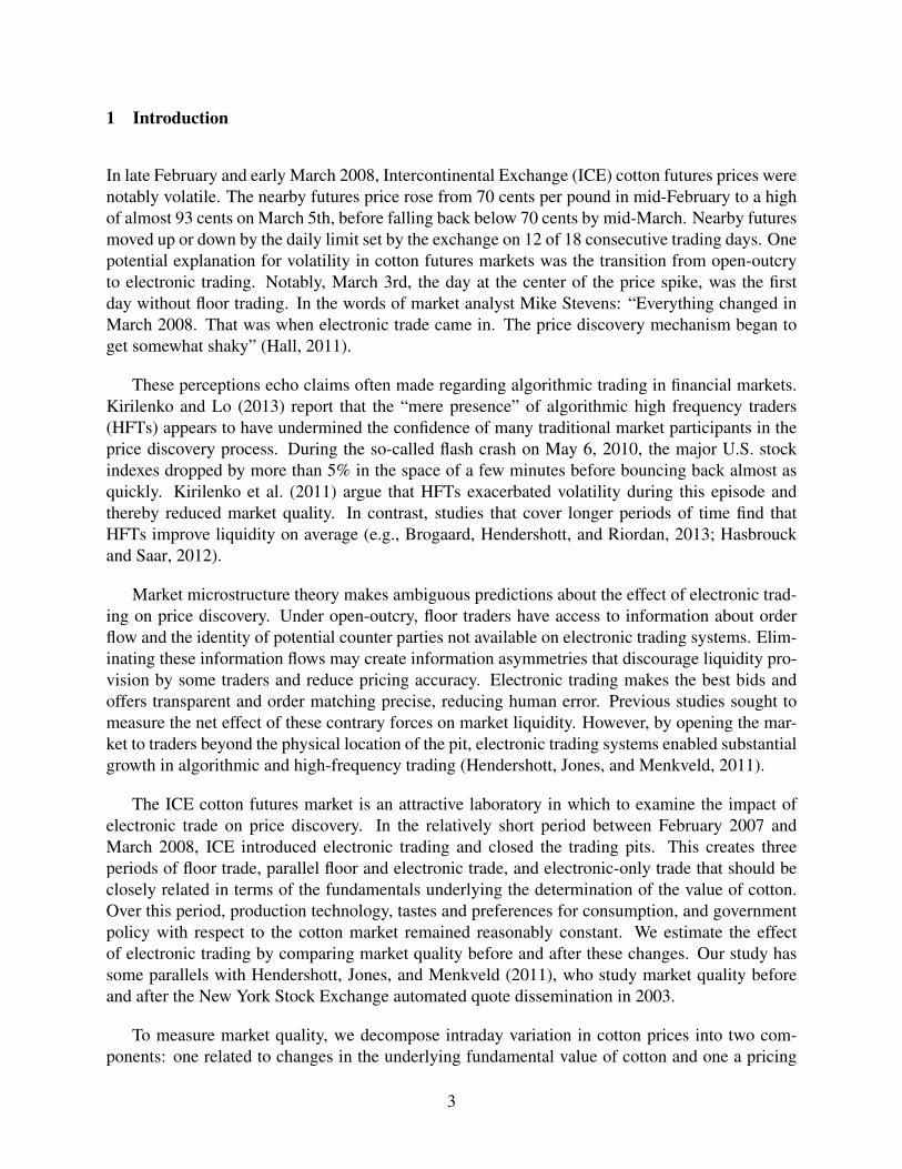
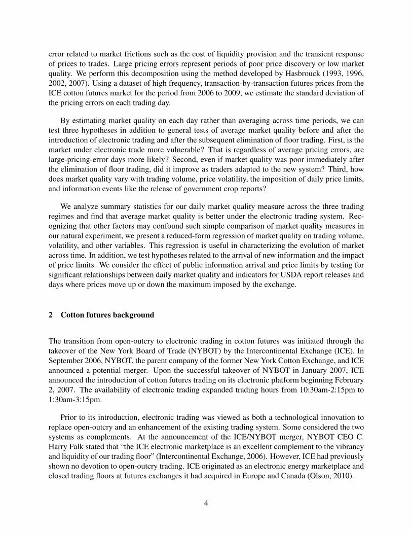
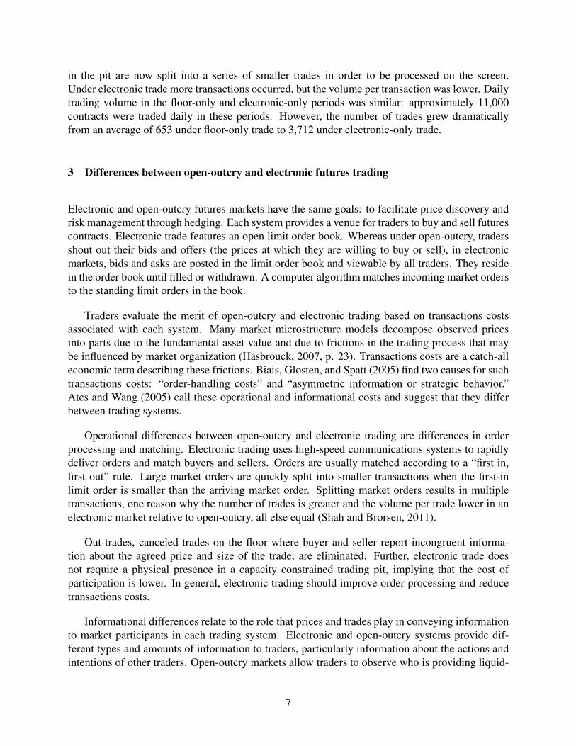
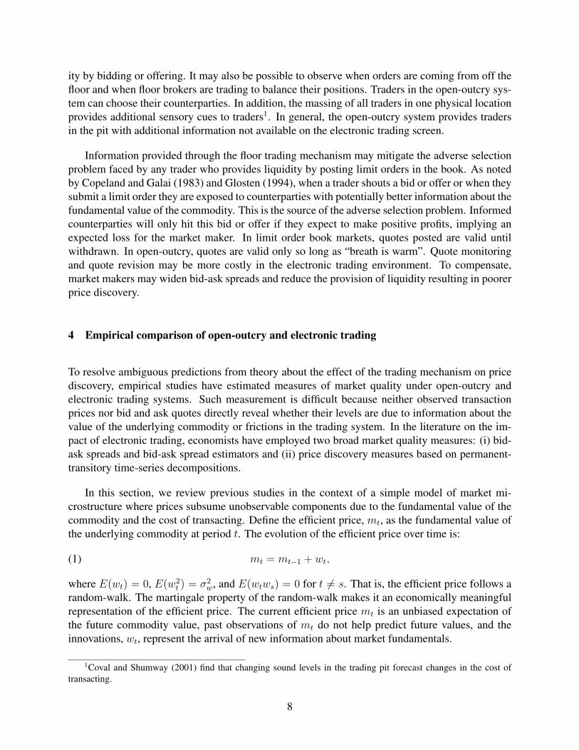
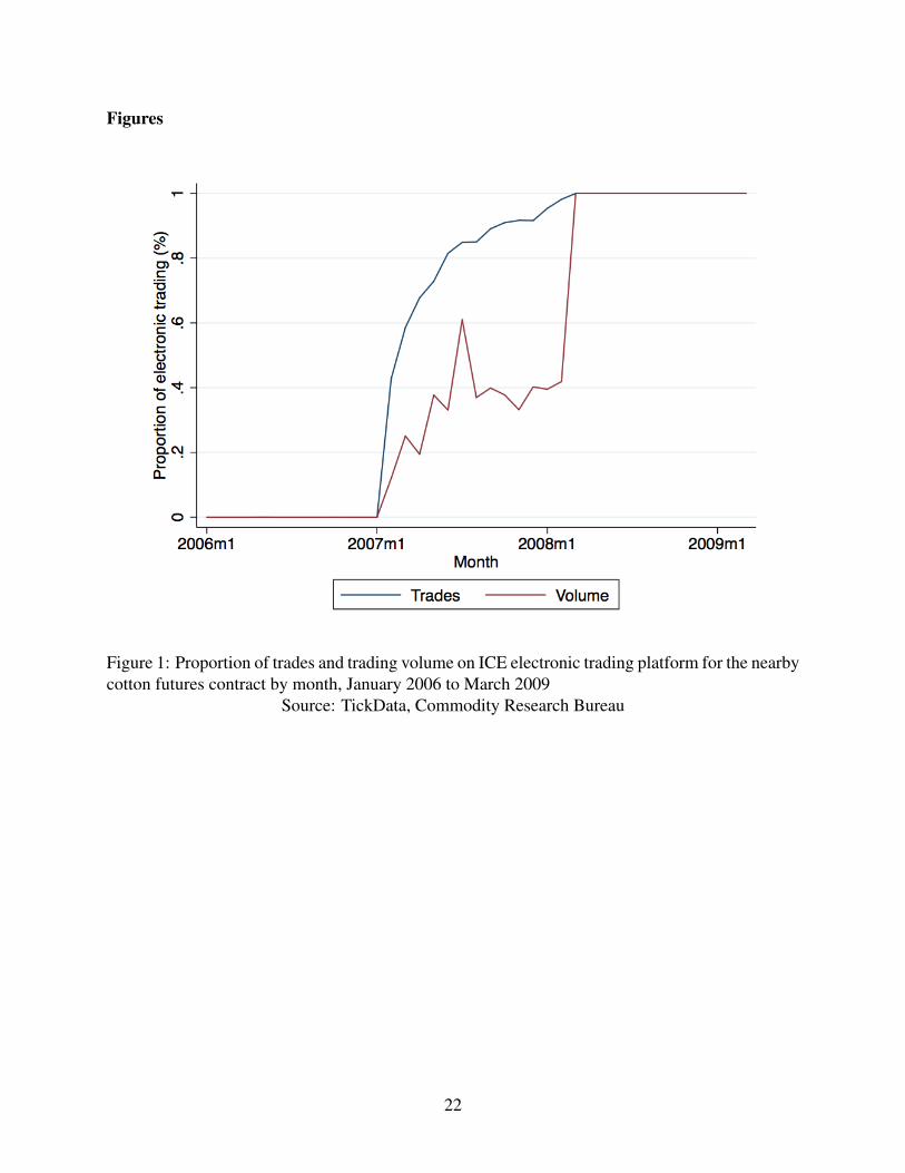
During 2007, cotton futures trading volume migrated to the electronic platform. Figure 1 showsthe increasing proportion of both monthly trading volume and number of trades on the electronicplatform in 2007. By July 2007, approximately 40% of trading volume and over 80% of tradesoccurred via electronic trading. As shown in figure 2, the absolute number of trades and tradingvolume both increased in 2007, with relatively larger increases in the number of trades. Tradingvolume fell after March 2008, but the number of trades remained high relative to historic levels.Volume per trade declined considerably following the introduction of electronic trading.

In December 2007, ICE announced it would close the cotton trading floor, effective Monday,March 3, 2008. The weeks preceding and following March 3, 2008 were a period of considerablecotton futures price volatility culminating in a sharp spike in cotton futures prices peaking March5. During this time, prices moved up or down the daily limit set by the exchange on 12 of 18consecutive trading days. When daily price limits are hit, trading stops until the following tradingday or until traders are willing to transact at prices inside the limit.

In the aftermath of the March 2008 price spike, some observers drew connection betweenextraordinary price changes and the elimination of floor trading. A Wall Street Journal reportnoted that in midst of limit moves on March 3rd and 4th, “frantic investors wondered where pricepressure was coming from. But with no more floor traders to consult for scuttlebutt, they werein the dark” (Davis, 2008). These remarks corroborate the idea that floor traders may play animportant role in incorporating fundamental information into commodity prices and transferringthat information to other market observers.

However, given the small proportion of trading on floor just prior to March 2008 (see figure 1),it seems unlikely that many traders and market observers were wholly reliant on the trading floor.Nor did the elimination of floor trading coincide with declining numbers of traders. Each weekthe Commodity Futures Trading Commission reports the number of “reportable” traders who holdlarge positions in each futures market. The number of large traders in ICE cotton futures betweenJune 2006 and October 2008 was consistently between 250 and 300 traders. The number of largetraders declined during the financial crisis in late 2008 by approximately 30-35% but similar de-clines were seen in other agricultural futures markets (Commodity Futures Trading Commission,2013).

In response to the events of March 2008 in the cotton futures market, the Commodity FuturesTrading Commission issued a report that considered “...the trading patterns of market participants,the broad increase in commodity prices in general, the impact of the presence of certain marketparticipants in the market, the possible tightening of credit conditions, the impact of price limitsin general, and the potential that prices may have been manipulated” (Commodity Futures TradingCommission, 2010). They concluded that trading and price patterns in cotton were not consistentwith any sort of market manipulation and that the elimination of floor trading was only coincidentalto observed price volatility, not the cause.

5

2.1 Daily cotton futures trading summary statistics across trading periods

Based on the history of the adoption of electronic trading in cotton futures, we consider threeperiods: floor trade, parallel floor and electronic trade, and electronic-only trade. The paralleltrade period contains 269 trading days between February 2, 2007 and February 29, 2008. Weselect a similar number of floor-only and electronic-only trading days to complete our dataset. Thefloor-only period is January 3, 2006 to February 1, 2007. The electronic-only period is March 3,2008 to March 27, 2009.

We identify important dates in the daily time series related to the arrival of public informationand exchange-imposed limits to price movement. We create indicator variables for days whereUSDA releases important information on cotton supply and demand conditions. The report dayvariable equals one on days when the USDA releases its monthly World Agricultural Supply andDemand Estimates and the annual Prospective Planting reports. During our study period, thesereports were released at 8:30am so prices could react to report information on the day of release.We also create indicators for days where prices move up or down daily limits. According to ICEcontract specifications during our study period, cotton futures could not trade more than three centshigher or lower than the previous day’s closing price when that price is below 84 cents per pound.Above 84 cents, the daily limit was four cents.

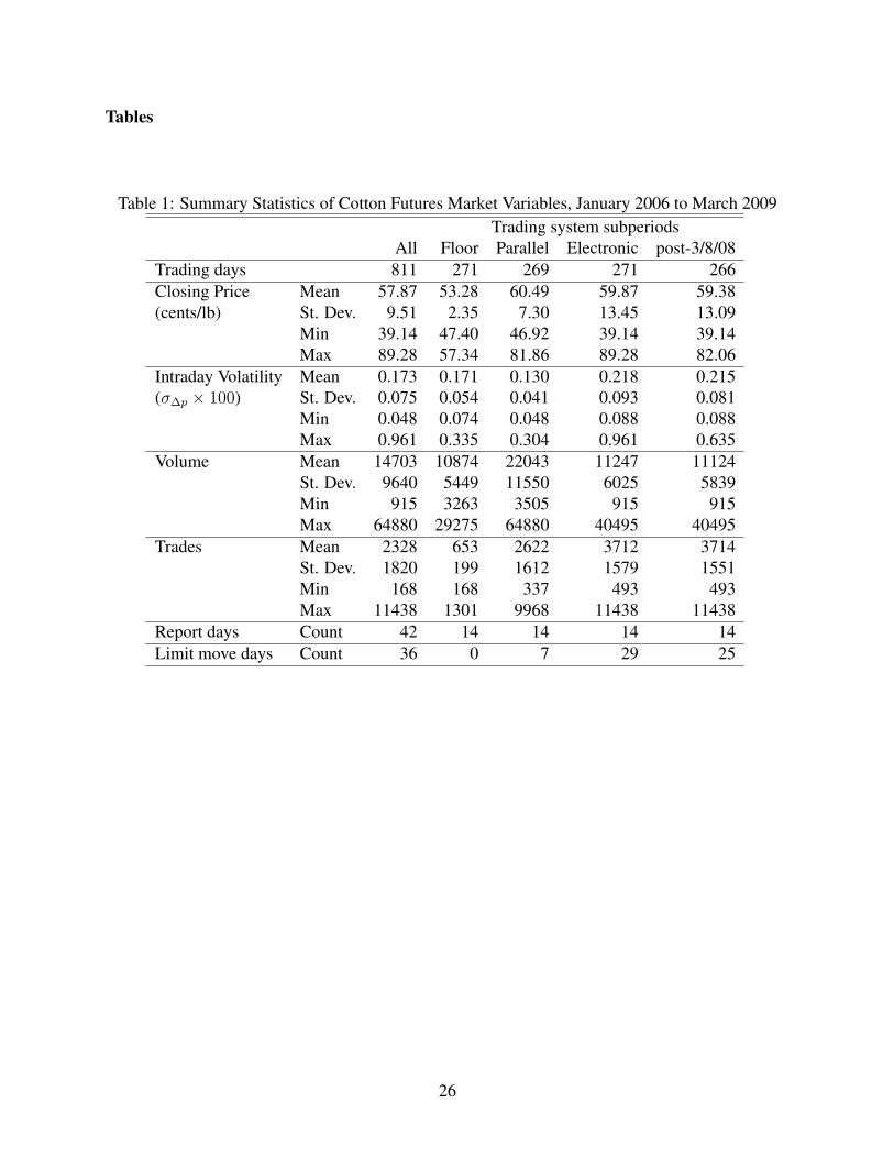
Table 1 presents summary statistics for daily data on prices, price volatility, trading volume,and the number of trades for the entire sample and the three subperiods of floor-only, parallelfloor and electronic, and electronic-only trade. In light of the extraordinary market conditions inthe week March 3, 2008, we calculate separate summary statistics for the electronic-only periodexcluding this week. We also present counts for the number of USDA report days and limit pricemove days within each period.

The results in table 1 suggest that market conditions varied across the three periods in oursample. While mean price levels were generally similar, price volatility increased. The coefficientsof variation for closing cotton futures prices during floor, parallel, and electronic periods were 0.04,0.12, and 0.22, respectively. A fivefold increase in relative standard deviation is dramatic, but otheragricultural commodity prices were also more volatile in 2008 than in 2006. Over the same March2008 to March 2009 period, corn, soybean, and wheat futures closing prices had similar coefficientsof variation (0.24, 0.21, and 0.25, respectively) though relative variability of closing prices onlydoubled or tripled compared to previous periods.

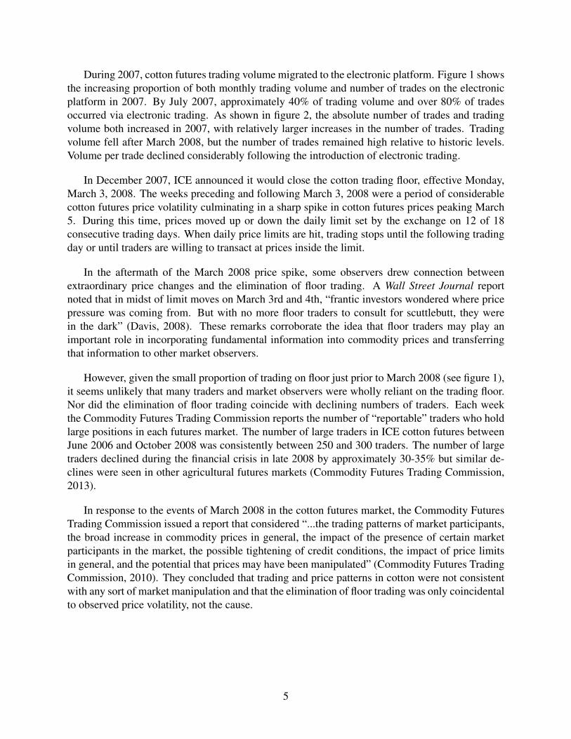
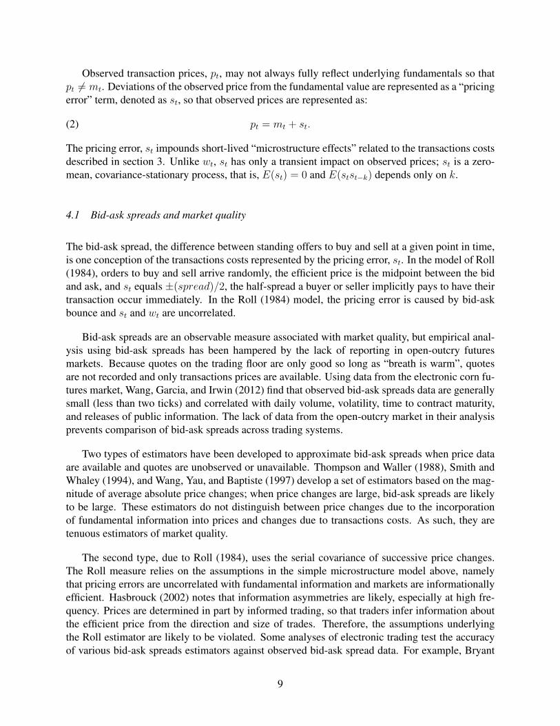
We consider intraday volatility using the standard deviation of log price changes over fiveminute intervals within the trading day. Table 1 shows intraday price volatility was greater andmore variable in the electronic-only period, though intraday volatility was actually lower duringthe parallel period than in the floor trading period. Figure 3 plots daily intraday price volatility forthe nearby cotton futures contract from January 2006 to March 2009. The pronounced spike in thisgraph occurs on March 4, 2008. Following this period of elevated volatility, intraday futures pricevolatility remained relatively high through the end of 2008 and early 2009.

Daily volume and trades statistics indicate that large market orders handled in a single trade

6

in the pit are now split into a series of smaller trades in order to be processed on the screen.Under electronic trade more transactions occurred, but the volume per transaction was lower. Dailytrading volume in the floor-only and electronic-only periods was similar: approximately 11,000contracts were traded daily in these periods. However, the number of trades grew dramaticallyfrom an average of 653 under floor-only trade to 3,712 under electronic-only trade.

3 Differences between open-outcry and electronic futures trading

Electronic and open-outcry futures markets have the same goals: to facilitate price discovery andrisk management through hedging. Each system provides a venue for traders to buy and sell futurescontracts. Electronic trade features an open limit order book. Whereas under open-outcry, tradersshout out their bids and offers (the prices at which they are willing to buy or sell), in electronicmarkets, bids and asks are posted in the limit order book and viewable by all traders. They residein the order book until filled or withdrawn. A computer algorithm matches incoming market ordersto the standing limit orders in the book.

Traders evaluate the merit of open-outcry and electronic trading based on transactions costsassociated with each system. Many market microstructure models decompose observed pricesinto parts due to the fundamental asset value and due to frictions in the trading process that maybe influenced by market organization (Hasbrouck, 2007, p. 23). Transactions costs are a catch-alleconomic term describing these frictions. Biais, Glosten, and Spatt (2005) find two causes for suchtransactions costs: “order-handling costs” and “asymmetric information or strategic behavior.”Ates and Wang (2005) call these operational and informational costs and suggest that they differbetween trading systems.

Operational differences between open-outcry and electronic trading are differences in orderprocessing and matching. Electronic trading uses high-speed communications systems to rapidlydeliver orders and match buyers and sellers. Orders are usually matched according to a “first in,first out” rule. Large market orders are quickly split into smaller transactions when the first-inlimit order is smaller than the arriving market order. Splitting market orders results in multipletransactions, one reason why the number of trades is greater and the volume per trade lower in anelectronic market relative to open-outcry, all else equal (Shah and Brorsen, 2011).

Out-trades, canceled trades on the floor where buyer and seller report incongruent informa-tion about the agreed price and size of the trade, are eliminated. Further, electronic trade doesnot require a physical presence in a capacity constrained trading pit, implying that the cost ofparticipation is lower. In general, electronic trading should improve order processing and reducetransactions costs.

Informational differences relate to the role that prices and trades play in conveying informationto market participants in each trading system. Electronic and open-outcry systems provide dif-ferent types and amounts of information to traders, particularly information about the actions andintentions of other traders. Open-outcry markets allow traders to observe who is providing liquid-

7

ity by bidding or offering. It may also be possible to observe when orders are coming from off thefloor and when floor brokers are trading to balance their positions. Traders in the open-outcry sys-tem can choose their counterparties. In addition, the massing of all traders in one physical locationprovides additional sensory cues to traders1. In general, the open-outcry system provides tradersin the pit with additional information not available on the electronic trading screen.

Information provided through the floor trading mechanism may mitigate the adverse selectionproblem faced by any trader who provides liquidity by posting limit orders in the book. As notedby Copeland and Galai (1983) and Glosten (1994), when a trader shouts a bid or offer or when theysubmit a limit order they are exposed to counterparties with potentially better information about thefundamental value of the commodity. This is the source of the adverse selection problem. Informedcounterparties will only hit this bid or offer if they expect to make positive profits, implying anexpected loss for the market maker. In limit order book markets, quotes posted are valid untilwithdrawn. In open-outcry, quotes are valid only so long as “breath is warm”. Quote monitoringand quote revision may be more costly in the electronic trading environment. To compensate,market makers may widen bid-ask spreads and reduce the provision of liquidity resulting in poorerprice discovery.

4 Empirical comparison of open-outcry and electronic trading

To resolve ambiguous predictions from theory about the effect of the trading mechanism on pricediscovery, empirical studies have estimated measures of market quality under open-outcry andelectronic trading systems. Such measurement is difficult because neither observed transactionprices nor bid and ask quotes directly reveal whether their levels are due to information about thevalue of the underlying commodity or frictions in the trading system. In the literature on the im-pact of electronic trading, economists have employed two broad market quality measures: (i) bid-ask spreads and bid-ask spread estimators and (ii) price discovery measures based on permanent-transitory time-series decompositions.

In this section, we review previous studies in the context of a simple model of market mi-crostructure where prices subsume unobservable components due to the fundamental value of thecommodity and the cost of transacting. Define the efficient price, mt, as the fundamental value ofthe underlying commodity at period t. The evolution of the efficient price over time is:

(1) mt = mt−1 + wt,

where E(wt) = 0, E(w2t ) = σ2

w, and E(wtws) = 0 for t 6= s. That is, the efficient price follows arandom-walk. The martingale property of the random-walk makes it an economically meaningfulrepresentation of the efficient price. The current efficient price mt is an unbiased expectation ofthe future commodity value, past observations of mt do not help predict future values, and theinnovations, wt, represent the arrival of new information about market fundamentals.

1Coval and Shumway (2001) find that changing sound levels in the trading pit forecast changes in the cost oftransacting.

8

Observed transaction prices, pt, may not always fully reflect underlying fundamentals so thatpt 6= mt. Deviations of the observed price from the fundamental value are represented as a “pricingerror” term, denoted as st, so that observed prices are represented as:

(2) pt = mt + st.

The pricing error, st impounds short-lived “microstructure effects” related to the transactions costsdescribed in section 3. Unlike wt, st has only a transient impact on observed prices; st is a zero-mean, covariance-stationary process, that is, E(st) = 0 and E(stst−k) depends only on k.

4.1 Bid-ask spreads and market quality

The bid-ask spread, the difference between standing offers to buy and sell at a given point in time,is one conception of the transactions costs represented by the pricing error, st. In the model of Roll(1984), orders to buy and sell arrive randomly, the efficient price is the midpoint between the bidand ask, and st equals ±(spread)/2, the half-spread a buyer or seller implicitly pays to have theirtransaction occur immediately. In the Roll (1984) model, the pricing error is caused by bid-askbounce and st and wt are uncorrelated.

Bid-ask spreads are an observable measure associated with market quality, but empirical anal-ysis using bid-ask spreads has been hampered by the lack of reporting in open-outcry futuresmarkets. Because quotes on the trading floor are only good so long as “breath is warm”, quotesare not recorded and only transactions prices are available. Using data from the electronic corn fu-tures market, Wang, Garcia, and Irwin (2012) find that observed bid-ask spreads data are generallysmall (less than two ticks) and correlated with daily volume, volatility, time to contract maturity,and releases of public information. The lack of data from the open-outcry market in their analysisprevents comparison of bid-ask spreads across trading systems.

Two types of estimators have been developed to approximate bid-ask spreads when price dataare available and quotes are unobserved or unavailable. Thompson and Waller (1988), Smith andWhaley (1994), and Wang, Yau, and Baptiste (1997) develop a set of estimators based on the mag-nitude of average absolute price changes; when price changes are large, bid-ask spreads are likelyto be large. These estimators do not distinguish between price changes due to the incorporationof fundamental information into prices and changes due to transactions costs. As such, they aretenuous estimators of market quality.

The second type, due to Roll (1984), uses the serial covariance of successive price changes.The Roll measure relies on the assumptions in the simple microstructure model above, namelythat pricing errors are uncorrelated with fundamental information and markets are informationallyefficient. Hasbrouck (2002) notes that information asymmetries are likely, especially at high fre-quency. Prices are determined in part by informed trading, so that traders infer information aboutthe efficient price from the direction and size of trades. Therefore, the assumptions underlyingthe Roll estimator are likely to be violated. Some analyses of electronic trading test the accuracyof various bid-ask spreads estimators against observed bid-ask spread data. For example, Bryant

9

and Haigh (2004) suggest that absolute average price change measures perform better than serialcovariance estimators at estimating spreads for their data on coffee and cocoa futures.

Three recent studies of electronic trade in agricultural commodity futures use these bid-askspread estimators, though they reach different conclusions. Bryant and Haigh (2004) consider theswitch to electronic trade in London International Financial Futures and Options Exchange cocoaand coffee futures in 2000. They find that average spreads are significantly larger under electronictrade than under open-outcry. In contrast, estimated bid-ask spreads are smaller for electronic trad-ing in studies of side-by-side open-outcry and electronic trading in Chicago Mercantile Exchange(CME) live cattle and live hog futures (Frank and Garcia, 2011), CME corn, wheat, and soybeansfutures (Martinez et al., 2011), and Kansas City Board of Trade wheat futures (Shah and Brorsen,2011). In each of these studies, reduced-form regressions measure the relationship between bid-askspreads and trading volume, observed price volatility, and other variables.

4.2 Random-walk decompositions and market quality

Random-walk decompositions based on the simple microstructure model discussed above are analternative to bid-ask spread estimation for the evaluation of market quality. These decompositionsare structural econometric models that allow us to characterize two unobserved but economicallymeaningful variables: the innovations in the random-walk, wt, representing information arrival andthe pricing error, st representing deviations from the efficient price due to transactions costs. Largepricing errors represent periods of poor discovery where observed prices are far from fundamen-tals. The standard deviation, σs and variance, σ2

s , of st are intuitive measures of market qualityrepresentative of the magnitude of deviations from the efficient price or an “average” pricing errorover some period of time.

Previous applications of random-walk decomposition methods to evaluate the transition fromopen-outcry to electronic trading divide their focus between wt and st. Studies focused on wt at-tribute some proportion of price discovery to the open-outcry or electronic market by consideringprices in each market as cointegrated time series whose innovations can be related to wt, the in-novations in a single efficient price relevant to both markets. The information shares technique ofHasbrouck (1995) and the common long-memory factor weights method of Gonzalo and Granger(1995) are used to measure the proportion of price discovery occurring in each market by identify-ing the proportion of the random-walk innovations (representing new information) first revealed inthe open-outcry or electronic market. Martinez et al. (2011) apply these methods to parallel open-outcry and electronic trading of Chicago Board of Trade agricultural futures contracts in 2006.Over this period, they find a growing proportion of price discovery occurred in electronic markets.

Multi-price decomposition methods are not suited to the comparison of market quality acrossperiods where trading occurs on some venues but not others. These methods necessarily compareprice discovery in related markets at a single point in time. However, trading tends to consolidatein a single venue (Silber, 1981) and open-outcry trading has been eliminated for some markets,so measuring a “share” of price discovery is not possible. We turn our focus to measuring themagnitude of the pricing error, st.

10

The pricing error captures deviations from the efficient price in both open-outcry and electronicmarkets. The structural model underlying the random-walk decomposition is agnostic with respectto specific mechanisms that generate observed sequences of trades. For example, we note abovethat the procedure for matching large incoming market orders differs between open-outcry andelectronic trades. To the extent that either trading system encourages a transient price response tothe incoming market order, our model will capture that transient response in the pricing error.

5 Identifying the pricing error variance through random-walk decomposition

In section 4, we characterized the dynamics of observed and efficient prices and made the case forthe pricing error standard deviation and variance as summary measures of market quality and theaccuracy of price discovery. To compare price discovery across the three periods of open-outcry,side-by-side, and electronic trading, we treat prices as a single time series whether transactions oc-cur on the trading floor or the electronic platform and compare the pricing error standard deviationacross periods. When open-outcry and electronic trading operated in parallel, contracts were fun-gible across the two platforms, traders in the pit had access to the electronic system, and settlementprices were determined by both open-outcry and electronic transactions.

Given the basic representation of the fundamental value and observed prices in equations 1 and2, Hasbrouck (1993, 2002, 2007) develops a statistical representation of the underlying microstruc-ture model that identifies the pricing error variance. The statistical model uses data on transactionprices, pt and trade direction, xt, a variable signed to be positive if the trader who initiated the tradeat time t is a buyer and negative if a seller. The data vector yt = [∆pt xt]

′ is presumed covariancestationary. By the Wold theorem, the data vector yt has a vector moving average representation:

(3) yt =

(∆pt

xt

)= Θ(L)εt

where

Θ(L)εt =

(Θ11(L) Θ12(L)Θ21(L) Θ22(L)

), Θ(0) = I, E[εtε

′t] = Ω =

(Ω11 Ω12

Ω21 Ω22

).

This statistical model simply states that price changes are a linear combination of current and pastshocks to price changes and trade direction. The covariance matrix, Ω, is unrestricted, so the twoshocks may be correlated.

The Beveridge and Nelson (1981) decomposition employed by Hasbrouck allows for iden-tification of permanent and transitory components in the VMA process. This method uses theautocorrelation structure of price changes and trade direction to identify the pricing error. By thisdecomposition, we can represent yt as:

yt = Θ(1)εt + Θ∗(L)∆εt.(4)= permanent + transitory

11

By taking the first difference of equation 2, price changes in the structural model can be expressedas ∆pt = wt + ∆st, where st is a mean zero, covariance stationary process. The correspondencebetween this representation and the first row of equation 4 implies:

wt = Θ11(1)ε1t + Θ12(1)ε2t(5)

st =m∑

i=1

(Θ∗11(L)∆ε1i + Θ∗12(L)∆ε2i) = Θ∗11(L)ε1i + Θ∗12(L)ε2i

Here wt is a linear combination of the two shocks and is white noise. The coefficients in Θ11(1)and Θ12(1) accumulate the current and future impacts of the present shocks and therefore representthe permanent effect of shocks on prices.

Hasbrouck (1993, 2007) follows standard time series practice in approximating the VMA(∞)in equation 4 with a finite VAR amenable to estimation:

(6) yt =

(∆pt

xt

)= φ1yt−1 + φ2yt−2 + · · ·+ φpyt−p + εt

where p is some lag length beyond which serial dependencies are assumed to be negligible. Usingthe VMA representation of the model, Hasbrouck (2007, Ch.9) derives the formula for the pricingerror variance:

σ2s =

∞∑k=0

CkΩC ′k(7)

where Ck = −∞∑

j=k+1

Θ1(j)

where Θ1(j) denotes the first row of Θ(j). The pricing error variance represents the magnitude ofthe deviations of the pricing error time series from its zero mean.

Including xt in the data vector yt strengthens the estimate of the pricing error variance. Sincethe permanent component is based on the forecast of the current and future impact of currentshocks, conditioning information will increase the precision of this forecast. According to Has-brouck (2007, pp. 87-88), xt is ideally a vector of public information used by traders to drawinference about mt over the relevant (very short run) time interval. For example, larger tradesmay contain more information than small ones (Holthausen, Leftwich, and Mayers, 1990). Omit-ting such information may bias coefficient estimates from the VAR model. Later we assess therobustness of our results to the inclusion of additional trade size information in xt.

As a measure of market quality, σ2s faces several complications. Lower values represent better

price discovery, so σ2s actually measures inverse market quality. σ2

s is a unitless measure, so itcannot be compared in terms similar to prices and spreads. To address these concerns and improvethe interpretation of our results, we refer to “market quality” as the negative standard deviation of

12

the pricing error:

(8) MQ = −√σ2

s .

Where we consider a logarithmic transformation of market quality, we express this as: lnMQ =− ln(

√σ2

s).

Tse and Zabotina (2001) apply the Hasbrouck (1993) methodology to assess market qualityin the transition to electronic trading. They study the transition of FTSE 100 stock index futuresfrom open-outcry to electronic trade in 1999. They calculate average standard deviation of thepricing error (σs) over two three-month trading periods before and after the switch and find thatthe floor-trade period is associated with higher market quality; the pricing error variance is lower inthis period. Our application of the Hasbrouck (1993) method considers more than average marketquality. We expand on previous studies by considering the evolution of market quality across time.

6 Estimation and results

Estimation of the Hasbrouck (1993) model requires data on two variables, returns and trade di-rection. We generate these variables using intraday tick-by-tick transaction data for ICE cottonfutures acquired from TickData Inc. This dataset records the time and price of each futures markettransaction. Transactions are time-stamped to the second. Electronic trades include the number ofcontracts exchanged; open-outcry trades do not report trade quantity. We supplement transaction-level data with daily price and volume information from the Commodity Research Bureau.

We consider transactions for one nearby contract each trading day rolling to the next contracton the twentieth day of the month prior to the delivery month. For cotton futures, the most-activenearby contract is usually the nearest to delivery, except for the October contract which is morelightly traded than the December contract. Therefore, we ignore the October contract and roll fromthe July to the December contract during the June roll period. We ignore natural time and treat thedata as an untimed sequence of observations. Returns are calculated as the log price change,ln(pt/pt−1), between the current and previous transaction so that t indexes transactions ratherthan clock time. Calculating returns in event time mitigates against heteroskedasticity in returnscaused by periods of frequent transactions. The covariance stationarity assumption underlying thestatistical model is more likely valid in event time (Hasbrouck, 2007).

Trade direction cannot be classified relative to quoted bids and offers because quote data isunavailable for the open-outcry period, so we cannot use the widely-used trade classification algo-rithm of Lee and Ready (1991). Instead, we employ a simple tick rule whereby the trade directionis classified as buyer-initiated if the previous price was lower than the transaction price and seller-initiated if the previous price was higher than the transaction price. When the previous price is thesame as the transaction price, the trade is classified the same as the previous trade classification.The trade direction variable, xt, is an indicator variable that takes on the value negative one whena trade is seller-initiated and one when a trade is buyer-initiated, following the tick rule outlinedabove. Though the tick rule considers less information than quote-based trade classification rules,

13

validation studies such as Ellis, Michaely, and O’Hara (2000) suggest that the difference in tradesmisclassified may not be large.

For each day in our sample. we estimate the VAR model for log returns, ∆pt, and trade direc-tion, xt presented in equation 6. Lag selection is based on Akaike (AIC) and Schwarz-Bayesian(SBIC) information criteria. We calculate optimal AIC and SBIC for each day. The average opti-mal AIC is slightly greater than four, so we use five lags2. Using the VAR results, we calculate theintraday pricing error variance using equation 7.

Market quality improved, but became more variable over the period of our analysis. Figure 4plots our market quality measure over the January 2006 to March 2009 period on a logarithmicscale. Vertical bars indicate the dates where electronic trading was introduced and floor tradingwas eliminated. Summary statistics for this series appear in table 2 for the full sample and thethree trading system regimes. Mean market quality improved from the floor-only to the electronic-only period. A simple t-test of the difference in means between the floor-only and electronic-onlyperiods finds that average market quality was significantly better under electronic-only trading.This improvement occurred gradually, beginning some time in the second quarter of 2007 afterelectronic trading gained a substantial share of trading volume.

Relative to the floor trading and parallel trading periods, market quality was more volatileduring the electronic trading period. The absolute value of the coefficient of variation for marketquality in the electronic-only period (excluding the week of March 3) was 0.697, nearly threetimes higher than during the floor period and nearly 50% higher than during the parallel period.We know that price volatility was also higher during these latter periods, however steadily growingdispersion of market quality about its trend in 2007 and into 2008 is not accompanied by similarsteady increases in intraday price volatility.

We find that market quality adapted quickly to the elimination of floor trading in March 2008.The period of the 2008 price spike was an outlier in terms of market quality as demonstrated by thefinal two columns of table 2. The minimum market quality statistic of -0.339 was calculated for theMarch 4, 2008 trading day. On this day, the nearby May 2008 cotton futures contract traded up thelimit most of the day. Excluding the period immediately surrounding the 2008 price spike showsthe impact of these outlier observations: without them the standard deviation of market qualityunder electronic trading was 0.008, the same as under floor-only trading.

Improved market quality over our period of analysis is prima facie evidence that the operationalefficiencies from electronic trading lead to improved price discovery. However, if some traders areparticularly sensitive to periods of poor price discovery, rising variability in market quality mayundermine confidence in the price discovery mechanism. Substantial variation in market qualitywithin each trading period argues for more detailed analysis using additional data on variablesrelated to the permanent and transitory components of observed prices identified in the Hasbrouckmodel.

2We also estimate the pricing error variance using the AIC-selected optimal lag length for each day. This does notsignificantly affect our results.

14

6.1 Incorporating trade size information

Hasbrouck (2007) suggested that including trade size in the data vector yt may convey additionalinformation about the fundamental value because large orders have greater information content.Our data do not contain trade size information for floor trades, but we incorporate the trade volumeinformation we do have to assess the robustness of our results to the exclusion of trade size data.We calculate an average daily trade size for floor trades by dividing daily floor trading volume bythe number of floor trades on that day. We replace the missing trade size values for each floor tradewith the average daily trade size for that day. Using this information, we can generate additionaltrade classification variables to incorporate what trade size data is available and incorporate theminto the VAR model.

Call the binary trade direction variable x1t. We generate x2t, the volume-weighted tradedirection by multiplying trade size (or average daily size for floor trades) by x1t. To capturenon-linearities in the response of price to trade size, Hasbrouck (2007) suggests also using thesquare root of x2t, or x3t. We estimate daily MQ using the four-variable VAR where yt =[∆pt x1t x2t x3t]

′. For the floor-only trading period, the variables xit are perfectly collinear,so the second and third variables are dropped from estimation and the MQ results are the same asour initial estimation procedure.

Additional trade size information does not substantially alter our results. Table 3 presents thesame summary statistics for market quality as in table 2. Summary statistics for the floor tradingperiod remain the same since we have no additional trade size information for this period. We findthat including additional information lowers average market quality and reduces relative variability.The magnitude of the change in means (0.02) is small relative to the differences in means acrossperiods.

6.2 Reduced-form regression results

Comparisons of market quality across trading systems in our sample may be confounded bychanges in other jointly determined variables. We employ a reduced-form regression analysisto consider how market quality changed holding these other variables constant. The regressions donot estimate causal impacts but simply describe associations present in the data. We present fivesimple linear regression specifications in table 4 where the dependent variable is the logarithm ofthe daily market quality, lnMQ. We also transform continuous control variables using logarithms.These transformations dampen the effects of outliers such as the March 2008 period and allowregression coefficients to be interpreted as approximate percentage changes.

The regression results confirm our univariate analysis of market quality. We find that marketquality was significantly better under electronic trading. The first specification in table 4 controlsfor changes in number of trades, volume, intraday price volatility, and days to contract maturity.We find that market quality is 18% better under electronic trading relative to other periods. Thisestimate is statistically significant at the 95% confidence level. Volatility and the number of trades

15

are significantly related to market quality; high volatility implies poorer price discovery. Specifi-cation (2) shows that our estimate of the impact of electronic trading on market quality is robust tothe inclusion of controls for report days and limit move days. In specifications (2), (4), and (5), themagnitude of the electronic trading effect on market quality is between 20 and 22%.

We find that inclusion of the number of trades variable in the regression equation greatly affectsthe results. Comparing specifications (2) and (3) in 4, the coefficient on the electronic trade indi-cator increases dramatically in (3). The coefficient for trading volume also becomes statisticallysignificant. Much of the benefit of electronic trading for improved market quality appears to beassociated with the increased number of trades. As we noted in section 3, the limit order bookelectronic market is more likely to break large orders into smaller transactions. At first appear-ances, the ability to quickly match large orders with the best available bids and offers may be partof the operational benefits associated with the electronic market. However, electronic trading isassociated with improved market quality even controlling for the number of trades.

Understanding how our structural model reacts to market order splitting under electronic trademay provide some additional explanation for the effect of the number of trades. Suppose theefficient price remains constant; a single buy order in an electronic market leads to some numberof small transactions at prices progressively further from the efficient price as the order is “walkedup the book”. In a floor market, the market order is more likely to result in a single transaction thatmay take longer to be matched but all else equal, the price impact of the trade is the same. Sincethe market price reverts to the constant efficient value in this example, our model assigns bothprice changes to the transitory component with similar implications for the pricing error variance.However, since our model cannot conclusively establish causal inference with respect to decreasedvolume per trade, we leave this for future work.

Market quality on USDA report days and limit move days

Specifications (2) and (4) allow us to consider the impact of public information arrival as repre-sented by USDA report days on market quality. According to our simplest specification, (2), wefind market quality is 11% better on USDA report days. In the context of our structural model,price changes on report days are more likely to reflect the permanent component associated withinformation arrival about the efficient price. USDA reports contain supply and demand data shownto have market impacts at lower frequency (e.g., McKenzie, 2008; Adjemian, 2012).

These results are consistent with the finance literature on public information disclosure and liq-uidity beginning with Diamond and Verrecchia (1991) and Kim and Verrecchia (1994). This liter-ature suggests that disclosure reduces information asymmetry between informed and uninformedtraders and reduced asymmetry leads to improved price discovery. USDA report days representperiods where commodities traders evaluate similar information, so information asymmetries, apotential source of transactions costs, are reduced on these days. Specification (4) also considersmarket quality on the day immediately prior to release days, finding poorer market quality on thesedays. Information asymmetries may be particularly acute on pre-report days where traders withheterogeneous expectations attempt to position themselves in advance of the report release.

16

We also estimate the impact of limit move days on market quality using specifications (2) and(4). We find limit move days are associated with a statistically significant 34% reduction in marketquality. When prices move up or down the limit and the efficient price change exceeds price lim-its, informed traders cannot incorporate their information into observed prices and market qualitysuffers. Any trading that does occur is likely due inventory control and margin call concerns3 notassociated with permanent shocks to observed prices.

Kyle (1988) suggests that price limits, when applied, may actually create greater uncertaintyabout the fundamental value. Later studies consider whether price limits reduce price volatility andassess the potential for price volatility on limit move days to spill over to subsequent trading days(e.g., Kim and Rhee, 1997). In specification (4), we find that days following limit move days arenot associated with statistically significant differences in market quality relative to other non-limitmove days.

We test whether market reaction to public information arrival changes after electronic tradingwas introduced by including an interaction between the USDA report day and electronic trading in-dicators in specification (5). We find improved market quality, though our coefficient estimates arenot statistically significant. We conduct a similar test of the effect of price limits in the presence ofelectronic trading by including a limit move-electronic trading interaction term. This specificationshows that the impact of price limits on market quality is greater under electronic trading, but thecoefficient on the limit move days indicator is no longer statistically significant. Generally, infor-mation arrival and price limit impacts appear to be magnified under electronic trading though theseestimates are not statistically significant. Given the length of our sample period, there may simplynot be enough report days or limit move days in our sample to precisely estimate the magnitude ofthese effects.

7 Discussion and conclusions

We find that the introduction of electronic trade has improved the quality of price discovery in theICE cotton futures market. Using random-walk decomposition methods, we define market qualityusing the variance of deviations from an unobserved efficient price. Lower variance of this pricingerror represents better market quality and more accurate price discovery. We find market quality islower during the electronic-only trading period than during the periods of floor-only and parallelfloor and electronic trade.

The elimination of floor trading for cotton futures coincided with a period of volatile pricesand high trading volume. Measured market quality at the height of the volatile price period waspoor, but our results do not find any relationship between lower market quality and electronic trade.Market quality improved significantly in the months that followed the introduction of electronictrading. It appears that traders adapted to the new system and did so quickly. Given the volume oftrade that had moved to the electronic platform before the elimination of open-outcry trading, this

3Carter and Janzen (2009) review the events surrounding the 2008 cotton price spike and discuss the extraordinarymargin call risk faced by cotton futures traders at a time when limit price moves were frequent.

17

result is not surprising.

Improved market quality under electronic trading is robust to changes across time in the levelof trading volume, price volatility, and the number of trades. Regression analysis estimates an 18-22% increase in market quality during the first 13 months of electronic trading in cotton futures,relative to the 25 preceding months. Our results also show that the relative variance of marketquality increased upon the elimination of floor trading. This result suggests that criticism of cottonfutures price discovery post-March 2008 may be driven by variability of price discovery rather thanchanges in the level of market quality. Traders sensitive to variability in the price discovery processmay be skeptical of purported benefits of electronic trading. Similar skepticism of algorithmic andhigh frequency trading may have the same cause.

Our analysis of market quality in the cotton futures market does not establish a specific, causallink between the electronic trading mechanism and market quality or the variability of marketquality. We do observe more transactions during the electronic-only period, consistent with thesplitting of large orders into smaller transactions than were previously matched on the tradingfloor. Our regression results point to a significant relationship between the number of trades andmarket quality. Whether dealing in smaller volume per trade helps traders tighten bid-ask spreadsor reduces costs related to adverse selection is an open empirical question. Further analysis ofprice discovery dynamics under electronic, algorithmic, and high frequency trading should explorethe relationship between volume per trade and market quality.

18

References

Adjemian, M.K. 2012. “Quantifying the WASDE Announcement Effect.” American Journal ofAgricultural Economics 94:238–256.

Ates, A., and G.H.K. Wang. 2005. “Information transmission in electronic versus open-outcrytrading systems: An analysis of U.S. equity index futures markets.” Journal of Futures Markets25:679–715.

Beveridge, S., and C.R. Nelson. 1981. “A new approach to decomposition of economic time se-ries into permanent and transitory components with particular attention to measurement of the‘business cycle’.” Journal of Monetary Economics 7:151 – 174.

Biais, B., L. Glosten, and C. Spatt. 2005. “Market microstructure: A survey of microfoundations,empirical results, and policy implications.” Journal of Financial Markets 8:217 – 264.

Brogaard, J., T. Hendershott, and R. Riordan. 2013. “High Frequency Trading and Price Discov-ery.” Working paper, University of California, Berkeley, April.

Bryant, H.L., and M.S. Haigh. 2004. “Bid-ask spreads in commodity futures markets.” AppliedFinancial Economics 14:923.

Carter, C.A., and J.P. Janzen. 2009. “The 2008 Cotton Price Spike and Extraordinary HedgingCosts.” Agricultural and Resource Economics Update 13:9–11.

Commodity Futures Trading Commission. 2013. “Disaggregated Commitment of Traders Report.”Data and explanatory notes, Washington, DC.

—. 2010. “Staff Report on Cotton Futures and Option Market Activity During the Week of March3, 2008.” Staff report, Washington, DC, January.

Copeland, T.E., and D. Galai. 1983. “Information Effects on the Bid-Ask Spread.” The Journal ofFinance 38:1457–1469.

Coval, J.D., and T. Shumway. 2001. “Is Sound Just Noise?” The Journal of Finance 56:1887–1910.

Davis, A. 2008. “In Mystery Cotton-Price Spike, Traders Hit by Swirling Forces.” Wall StreetJournal, August 13, pp. A1.

Diamond, D.W., and R.E. Verrecchia. 1991. “Disclosure, Liquidity, and the Cost of Capital.” TheJournal of Finance 46:1325–1359.

Ellis, K., R. Michaely, and M. O’Hara. 2000. “The Accuracy of Trade Classification Rules: Evi-dence from Nasdaq.” The Journal of Financial and Quantitative Analysis 35:529–551.

Frank, J., and P. Garcia. 2011. “Bid-ask spreads, volume, and volatility: Evidence from livestockmarkets.” American Journal of Agricultural Economics 93:209–225.

Glosten, L.R. 1994. “Is the Electronic Open Limit Order Book Inevitable?” The Journal of Finance49:1127–1161.

19

Gonzalo, J., and C. Granger. 1995. “Estimation of Common Long-Memory Components in Coin-tegrated Systems.” Journal of Business and Economic Statistics 13:27–35.

Hall, K.G. 2011. “Speculators drive cotton price volatility, hurting farmers and consumers.” Mc-Clatchy Washington Bureau, November 30, pp. –.

Hasbrouck, J. 1993. “Assessing the quality of a security market: a new approach to transaction-costmeasurement.” Review of Financial Studies 6:191–212.

—. 2007. Empirical market microstructure: The institutions, economics and econometrics of se-curities trading. New York, NY: Oxford University Press.

—. 1996. “Modeling Microstructure Time Series.” In G. Maddala and C. Rao, eds. Handbook ofStatistics. Elsevier Science, vol. 16, chap. 22, pp. 647–692.

—. 1995. “One Security, Many Markets: Determining the Contributions to Price Discovery.” TheJournal of Finance 50:pp. 1175–1199.

—. 2002. “Stalking the “efficient price” in market microstructure specifications: an overview.”Journal of Financial Markets 5:329 – 339.

Hasbrouck, J., and G. Saar. 2012. “Low-Latency Trading.” Working Paper No. 35-2010, JohnsonSchool Research Paper Series, December.

Hendershott, T., C.M. Jones, and A.J. Menkveld. 2011. “Does Algorithmic Trading Improve Liq-uidity?” The Journal of Finance 66:1–33.

Holthausen, R.W., R.W. Leftwich, and D. Mayers. 1990. “Large-block transactions, the speed ofresponse, and temporary and permanent stock-price effects.” Journal of Financial Economics26:71 – 95.

Intercontinental Exchange. 2006. “Intercontinental Exchange Proposed Acquisition Overwhelm-ingly Approved In Vote By NYBOT Members.” Press release, New York, NY, December.

Kim, K.A., and S.G. Rhee. 1997. “Price Limit Performance: Evidence from the Tokyo StockExchange.” The Journal of Finance 52:885–901.

Kim, O., and R.E. Verrecchia. 1994. “Market liquidity and volume around earnings announce-ments.” Journal of Accounting and Economics 17:41 – 67.

Kirilenko, A.A., A.S. Kyle, M. Samadi, and T. Tuzun. 2011. “The Flash Crash: The Impact ofHigh Frequency Trading on an Electronic Market.” Working paper, Commodity Futures TradingCommission, May.

Kirilenko, A.A., and A.W. Lo. 2013. “Moore’s Law versus Murphy’s Law: Algorithmic Tradingand Its Discontents.” Journal of Economic Perspectives 27(2):51–72.

Kyle, A. 1988. “Trading halts and price limits.” Review of Futures Markets 7:426–434.

20

Lee, C.M.C., and M.J. Ready. 1991. “Inferring Trade Direction from Intraday Data.” The Journalof Finance 46:pp. 733–746.

Martinez, V., P. Gupta, Y. Tse, and J. Kittiakarasakun. 2011. “Electronic versus open outcry tradingin agricultural commodities futures markets.” Review of Financial Economics 20:28–36.

McKenzie, A.M. 2008. “Pre-Harvest Price Expectations for Corn: The Information Content ofUSDA Reports and New Crop Futures.” American Journal of Agricultural Economics 90:351–366.

Olson, E.S. 2010. Zero Sum Game: The Rise of the World’s Largest Derivatives Exchange. Hobo-ken, NJ: Wiley.

Roll, R. 1984. “A Simple Implicit Measure of the Effective Bid-Ask Spread in an Efficient Market.”The Journal of Finance 39:1127–1139.

Shah, S., and W. Brorsen. 2011. “Electronic vs. Open Outcry: Side-by-Side Trading of KCBTWheat Futures.” Journal of Agricultural and Resource Economics 36:48–62.

Silber, W.L. 1981. “Innovation, competition, and new contract design in futures markets.” Journalof Futures Markets 1:123 – 155.

Smith, T., and R.E. Whaley. 1994. “Estimating the effective bid/ask spread from time and salesdata.” Journal of Futures Markets 14:437–455.

Thompson, S.R., and M.L. Waller. 1988. “Determinants of Liquidity Costs in Commodity FuturesMarkets.” Review of Futures Markets 7:110– 126.

Tse, Y., and T.V. Zabotina. 2001. “Transaction Costs and Market Quality: Open Outcry VersusElectronic Trading.” Journal of Futures Markets 21:713–735.

Wang, G.H.K., J. Yau, and T. Baptiste. 1997. “Trading volume and transaction costs in futuresmarkets.” Journal of Futures Markets 17:757–780.

Wang, X., P. Garcia, and S.H. Irwin. 2012. “The Behavior of Bid-Ask Spreads in the Electroni-cally Traded Corn Futures Market.” In Proceedings of the NCCC-134 Conference on AppliedCommodity Price Analysis, Forecasting and Risk Management. St. Louis, MO.

21

Figures

Figure 1: Proportion of trades and trading volume on ICE electronic trading platform for the nearbycotton futures contract by month, January 2006 to March 2009

Source: TickData, Commodity Research Bureau

22

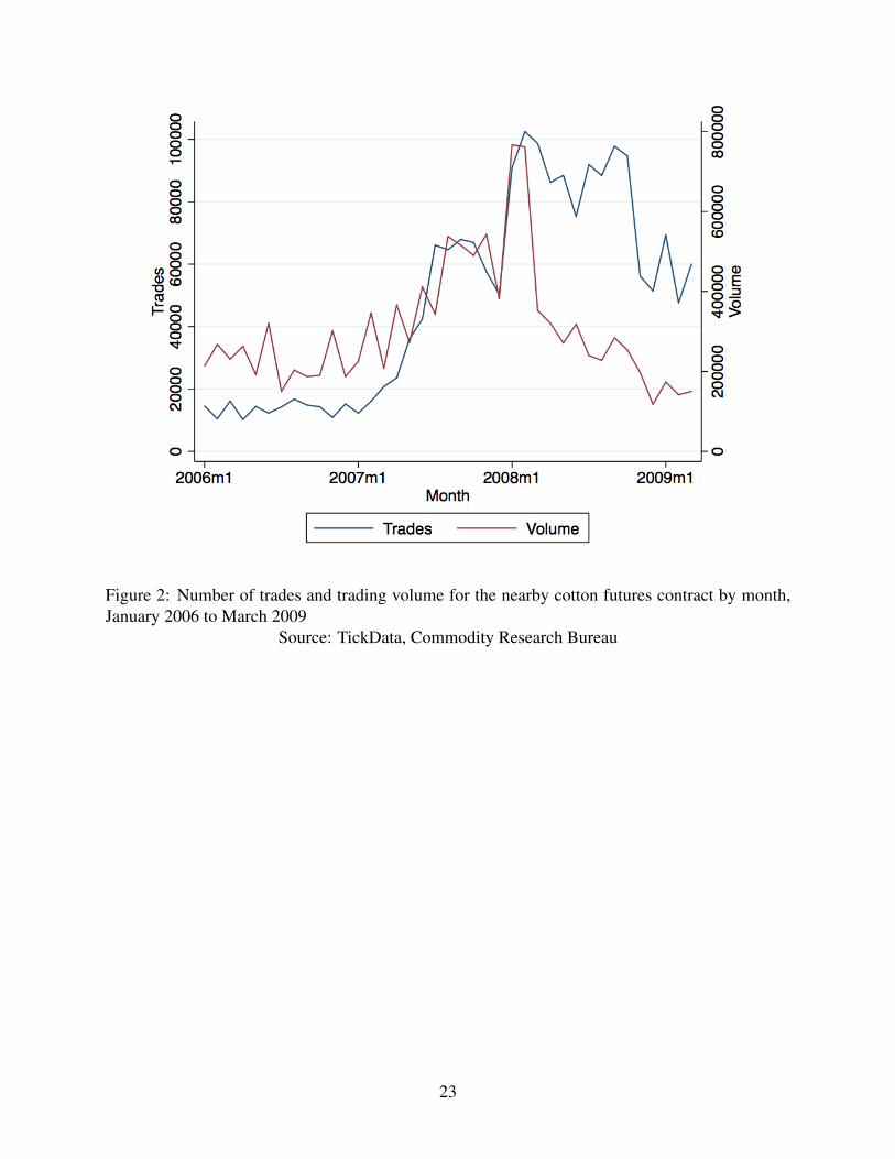
Figure 2: Number of trades and trading volume for the nearby cotton futures contract by month,January 2006 to March 2009

Source: TickData, Commodity Research Bureau

23

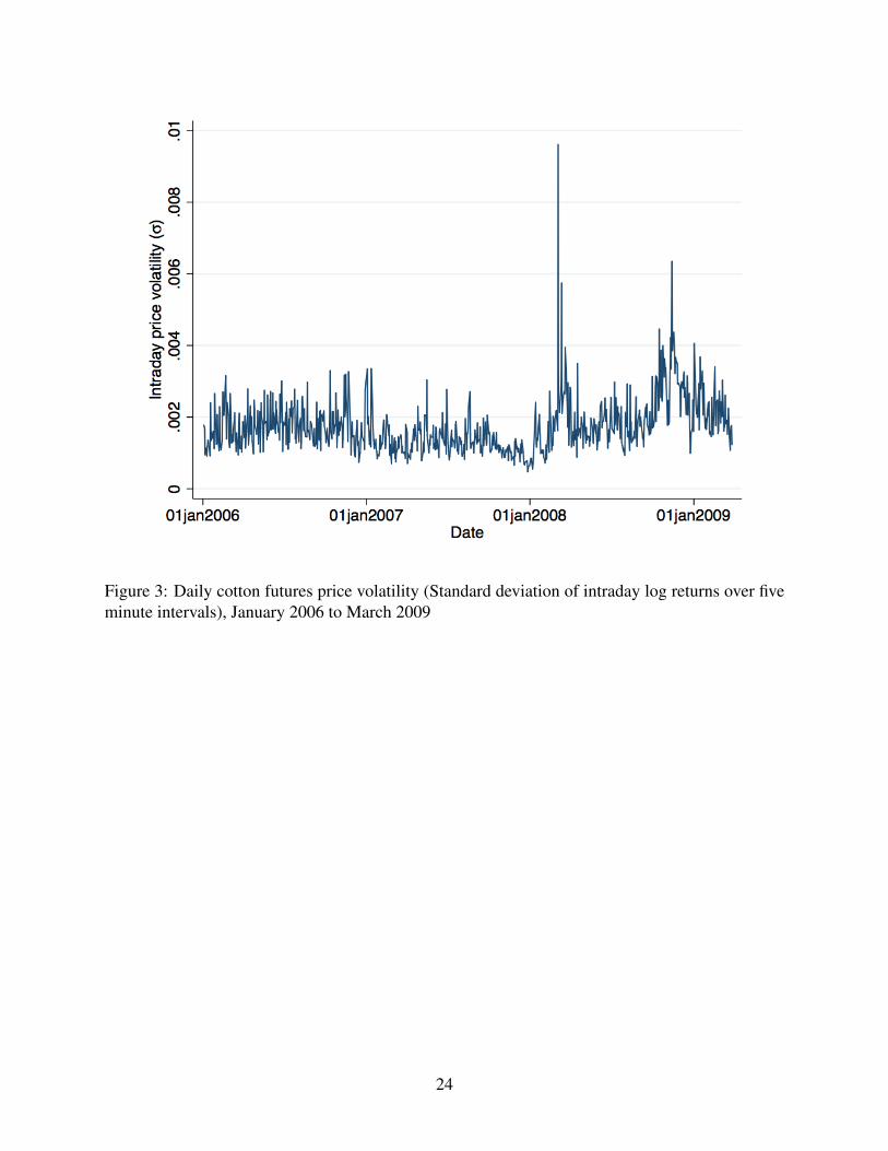
Figure 3: Daily cotton futures price volatility (Standard deviation of intraday log returns over fiveminute intervals), January 2006 to March 2009

24

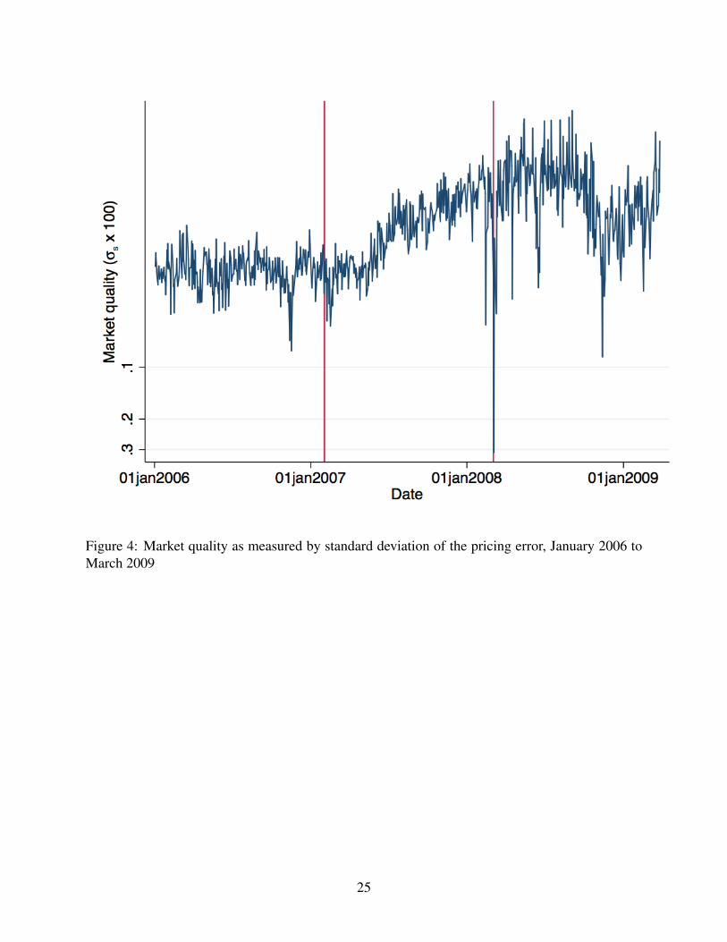
Figure 4: Market quality as measured by standard deviation of the pricing error, January 2006 toMarch 2009

25

Tables

Table 1: Summary Statistics of Cotton Futures Market Variables, January 2006 to March 2009Trading system subperiods

All Floor Parallel Electronic post-3/8/08Trading days 811 271 269 271 266Closing Price Mean 57.87 53.28 60.49 59.87 59.38(cents/lb) St. Dev. 9.51 2.35 7.30 13.45 13.09

Min 39.14 47.40 46.92 39.14 39.14Max 89.28 57.34 81.86 89.28 82.06

Intraday Volatility Mean 0.173 0.171 0.130 0.218 0.215(σ∆p × 100) St. Dev. 0.075 0.054 0.041 0.093 0.081

Min 0.048 0.074 0.048 0.088 0.088Max 0.961 0.335 0.304 0.961 0.635

Volume Mean 14703 10874 22043 11247 11124St. Dev. 9640 5449 11550 6025 5839Min 915 3263 3505 915 915Max 64880 29275 64880 40495 40495

Trades Mean 2328 653 2622 3712 3714St. Dev. 1820 199 1612 1579 1551Min 168 168 337 493 493Max 11438 1301 9968 11438 11438

Report days Count 42 14 14 14 14Limit move days Count 36 0 7 29 25

26

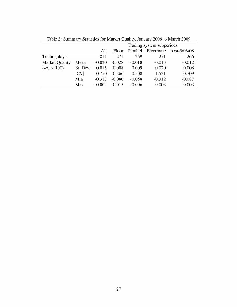
Table 2: Summary Statistics for Market Quality, January 2006 to March 2009Trading system subperiods

All Floor Parallel Electronic post-3/08/08Trading days 811 271 269 271 266Market Quality Mean -0.020 -0.028 -0.018 -0.013 -0.012(-σs × 100) St. Dev. 0.015 0.008 0.009 0.020 0.008

|CV| 0.750 0.266 0.508 1.531 0.709Min -0.312 -0.080 -0.058 -0.312 -0.087Max -0.003 -0.015 -0.006 -0.003 -0.003

27

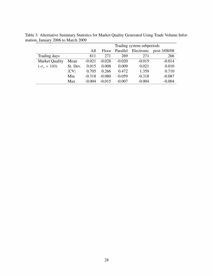
Table 3: Alternative Summary Statistics for Market Quality Generated Using Trade Volume Infor-mation, January 2006 to March 2009

Trading system subperiodsAll Floor Parallel Electronic post-3/08/08

Trading days 811 271 269 271 266Market Quality Mean -0.021 -0.028 -0.020 -0.015 -0.014(-σs × 100) St. Dev. 0.015 0.008 0.009 0.021 0.010

|CV| 0.705 0.266 0.472 1.359 0.710Min -0.318 -0.080 -0.059 -0.318 -0.087Max -0.004 -0.015 -0.007 -0.004 -0.004

28

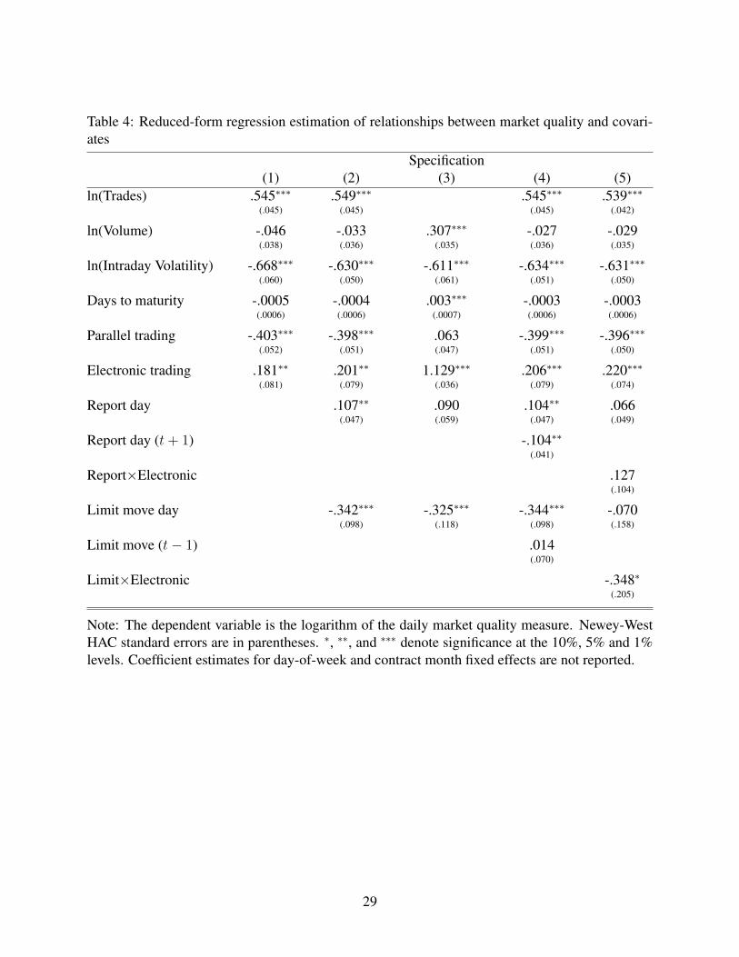
Table 4: Reduced-form regression estimation of relationships between market quality and covari-ates

Specification(1) (2) (3) (4) (5)

ln(Trades) .545∗∗∗ .549∗∗∗ .545∗∗∗ .539∗∗∗(.045) (.045) (.045) (.042)

ln(Volume) -.046 -.033 .307∗∗∗ -.027 -.029(.038) (.036) (.035) (.036) (.035)

ln(Intraday Volatility) -.668∗∗∗ -.630∗∗∗ -.611∗∗∗ -.634∗∗∗ -.631∗∗∗(.060) (.050) (.061) (.051) (.050)

Days to maturity -.0005 -.0004 .003∗∗∗ -.0003 -.0003(.0006) (.0006) (.0007) (.0006) (.0006)

Parallel trading -.403∗∗∗ -.398∗∗∗ .063 -.399∗∗∗ -.396∗∗∗(.052) (.051) (.047) (.051) (.050)

Electronic trading .181∗∗ .201∗∗ 1.129∗∗∗ .206∗∗∗ .220∗∗∗(.081) (.079) (.036) (.079) (.074)

Report day .107∗∗ .090 .104∗∗ .066(.047) (.059) (.047) (.049)

Report day (t+ 1) -.104∗∗(.041)

Report×Electronic .127(.104)

Limit move day -.342∗∗∗ -.325∗∗∗ -.344∗∗∗ -.070(.098) (.118) (.098) (.158)

Limit move (t− 1) .014(.070)

Limit×Electronic -.348∗(.205)

Note: The dependent variable is the logarithm of the daily market quality measure. Newey-WestHAC standard errors are in parentheses. ∗, ∗∗, and ∗∗∗ denote significance at the 10%, 5% and 1%levels. Coefficient estimates for day-of-week and contract month fixed effects are not reported.

29