Embed Size (px)
Citation preview

p
VfVp
fp
f ggg
202
2
02
The Quasi-Geostrophic Omega Equation (without friction and diabatic terms)
We will now develop the Trenberth (1978)* modification to the QG Omega equation
THE TRENBERTH (1978) INTERPRETATION
*Trenberth, K.E., 1978: On the Interpretation of the Diagnostic Quasi-Geostrophic Omega Equation. Mon. Wea. Rev., 106, 131–137
Trenberth (1978) argued that carrying out all of the derivatives on the RHS on the Equation could simplify the forcing function for .
PROBLEM: TERM 1 and 2 on the RHS are often large and opposite leading to ambiguity about the sign and magnitude of when analyzing weather maps

p
VfVp
fp
f ggg
202
2
02
py
vpx
uy
fv
x
fu
pf
p
fgg
gg
gg
222
02
202
QG OMEGA EQUATION:
EXPAND THE ADVECTION TERMS:
yfug
1xf
vg
1 2
0
1
fg
USE THE EXPRESSIONS FOR THE GEOSTROPHIC WIND AND GEOSTROPHIC VORTICITY:
To Get:
pyxpxyf
ffyxf
ffxyfp
fp
f
22
22
0
2
002
202 11111

pyxpxyf
ffyxf
ffxyfp
fp
f
22
22
0
2
002
202 11111
x
B
y
A
y
B
x
ABAJ ,
EXPAND ALL THE DERIVATIVESTHEN USE THE JACOBIAN OPERATOR TO SIMPLIFY NOTATION
RESULT:
212
202 1
FFfp
f
pyy
Jpxx
Jp
Jp
JF22
221 ,,2,,
p
Jffp
Jp
JF 2
02
2 ,,,

pyy
Jpxx
Jp
Jp
JF22
221 ,,2,,
p
Jffp
Jp
JF 2
02
2 ,,,
Same term:opposite sign
DeformationTerms in Sutcliff eqn
Trenberth: Ignore deformation terms (removes frontogenetic effects)
212
202 1
FFfp
f
Opposite term:opposite sign = same term
02
21 ,,211
ffp
Jp
Jf
FFf
02
21 ,,21
ffp
Jp
Jf
FFf
Approximate last term = 2 last term

02
21 ,,21
ffp
Jp
Jf
FFf
Expand Jacobian terms:
fp
Vf
p
fg
g
02
202 2
This result says that large scale vertical motions can be diagnosed by Examining the advection of absolute vorticity by the thermal wind
fVVVVf gg 000
RECALL SUTCLIFF’S EQUATION
SAME INTERPRETATION!!

The Geostrophic paradox
Confluent geostrophic flow will tighten
temperature gradient, leading to an increase in
shear via the thermal wind relationship……..
……but advection of geostrophic momentum
by geostrophic wind decreases the vertical shear in the column
so…geostrophic flow destroysgeostrophic balance!

00
aggg ufvVt
0
pV
t g
0
gg vVt
0
pV
t g
000
y
vv
x
vu
t
v
pfvV
tpf g
gg
gg
gg
y momentum equation (QG)
Thermodynamic energy equation (QG)
For the moment, let’s ignore the ageostrophy (no uag and no )
The geostrophic paradox: a mathematical interpretation
Take vertical derivative of first equation
Let’s look at this equation

000
y
vv
x
vu
t
v
pfvV
tpf g
gg
gg
gg
Expand the derivative:
0000
y
v
p
v
x
v
p
uf
p
vfV
tvV
tpf ggggg
ggg
Substitute using the thermal wind relationship:
pxp
vf g
2
0
000
px
V
p
vfV
tvV
tpf gg
ggg
to get:
pyp
uf g
2
0
Remember equation in blue box

00
aggg ufvVt
0
pV
t g
0
gg vVt
0
pV
t g
y momentum equation (QG)
Thermodynamic energy equation (QG)
For the moment, let’s ignore the ageostrophy (no uag and no )
The geostrophic paradox: a mathematical interpretation
Take x derivative of second equation
Now let’s look at this equation
0
py
vpx
uptxp
Vtx ggg

0
py
vpx
uptxp
Vtx ggg
Expand the derivative and use vector notation:
02
px
V
pxV
tpV
txg
gg
Now recall first saved equation:
000
px
V
p
vfV
tvV
tpf gg
ggg
Let’s take these two blue boxed equations and compare them…..

px
V
pxV
tg
g
2
px
V
p
vfV
tgg
g
0
pxp
vf g
2
0
Following the geostrophic wind themagnitude of the temperature gradientand the vertical shear have opposite
Tendencies
TIGHTENING THE TEMPERATURE GRADIENT WILL REDUCE THE SHEAR!
thermal windbalance

The Geostrophic paradox:
RESOLUTION
A separate “ageostrophiccirculation” must exist thatrestores geostrophic balance thatsimultaneously:
1) Decreases the magnitude of the horizontal temperature gradient
2) Increases the vertical shear
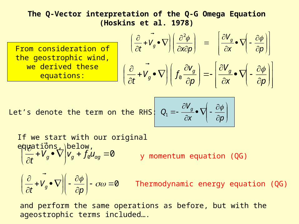
The Q-Vector interpretation of the Q-G Omega Equation(Hoskins et al. 1978)
px
V
pxV
tg
g
2
px
V
p
vfV
tgg
g
0
From consideration of the geostrophic wind, we derived
these equations:
Let’s denote the term on the RHS:
px
VQ g
1
00
aggg ufvVt
0
pV
t g
y momentum equation (QG)
Thermodynamic energy equation (QG)
If we start with our original equations, below,
and perform the same operations as before, but with the ageostrophic terms included….

We arrive at:
02010
p
ufQ
p
vfV
tagg
g
01
2
xQ
pxV
t g
01
2
Qpx
Vt g
010
Qp
vfV
tg
g
With ageostrophic terms
Only geostrophic terms
Note that the additional terms represent the ageostrophic circulation that works to reestablish geostrophic balance as air accelerates in unbalanced flow.

02010
p
ufQ
p
vfV
tagg
g
01
2
xQ
pxV
t g
With ageostrophic terms
Let’s multiply the bottom equation by -1 and add it to the top equation, recalling
that pyp
uf g
2
0
p
uf
xQ ag
2012
Let’s do the same operations with the x equation of motion and the thermodynamicequation. If we do, we find that:
p
vf
yQ ag
2022

Let’s do the same operations with the x equation of motion and the thermodynamicequation.
p
vf
yQ ag
2022
02020
p
vfQ
p
ufV
tagg
g
02
2
yQ
pxV
t g
py
VQ g
2Where:
and:

p
vf
yQ ag
2022
p
uf
xQ ag
2012
A
B
Takey
B
x
A
y
v
x
u
pf
yxy
Q
x
Q agag202
2
2
2212
2
2
02
2
2
2212
pf
yxy
Q
x
Q
Substitute continuity equation
And use vector notation to get:

y
Q
x
Q
pf 21
2
2
02 2
p
Vff
Vp
fp
fgg
22
002
2202 1
COMPARE THIS EQUATION WITH THE TRADITIONAL QG EQUATION!
Qp
f
22
2
02
We can write the Q-vector form of the QG equation as:
Where the components of the Q vector are
jpy
Vi
px
VQ gg ˆ,ˆ

jpy
Vi
px
VQ gg ˆ,ˆ
Using the hydrostatic relationship, we can write Q more simply as:
jTy
ViT
x
V
p
RQ gg ˆ,ˆ
jy
T
y
v
x
T
y
ui
y
T
x
v
x
T
x
u
p
RQ gggg ˆˆ
or in scalar notation as

02 Q
First note that if the Q vector is convergent
0 Q
Qp
f
22
2
02
02
2
02
p
f
0
Therefore air is rising when the Q vector is convergent

jy
T
y
v
x
T
y
ui
y
T
x
v
x
T
x
u
p
RQ gggg ˆˆ
Let’s go back to our jet entrance region
Note that there is no in this particular jety
T
jy
ui
y
v
x
T
p
Rj
x
T
y
ui
x
T
x
u
p
RQ gggg ˆˆˆ,ˆ
y
Vk
x
T
p
RQ g
ˆ
Q c
onve
rgen
ce
Q d
iver
genc
e
The Q vectors capture the sense of the ageostrophic circulation and allow us to see where the rising motion is occurring

y
Vk
x
T
p
RQ g
ˆ
Q c
onve
rgen
ce
Q d
iver
genc
e
The Q vectors capture the sense of the ageostrophic circulation and allow us to see where the rising motion is occurring
Q vectors diagnose a thermally direct circulation
Adiabatic cooling of rising warm air Adiabatic warming of sinking cold air
Counteracts the tendency of the geostrophictemperature advection in confluent flow
Under influence of Coriolis force, horizontalbranches tend to increase shear
Counteracts the tendency of the geostrophicMomentum advection in the confluent flow
Resolution of the Geostrophic Paradox

A natural coordinate version of the Q vector(Sanders and Hoskins 1990)
jy
T
y
v
x
T
y
ui
y
T
x
v
x
T
x
u
p
RQ gggg ˆˆ
Consider a zonally oriented confluent
entrance region of a jet where 0x
T
jy
vi
x
v
y
T
p
RQ gg ˆˆ
jx
ui
x
v
y
T
p
RQ gg ˆˆ
Use non-divergence of geostrophic wind
or
x
Vk
y
T
p
RQ g
ˆ

A natural coordinate version of the Q vector(Sanders and Hoskins 1990)
jy
T
y
v
x
T
y
ui
y
T
x
v
x
T
x
u
p
RQ gggg ˆˆ
Consider a meridionally oriented confluent
entrance region of a jet where 0y
T
jy
ui
x
u
x
T
p
RQ gg ˆˆ
jy
ui
y
v
x
T
p
RQ gg ˆˆ
Use non-divergence of geostrophic wind
or
y
Vk
x
T
p
RQ g
ˆ

A natural coordinate version of the Q vector(Sanders and Hoskins 1990)
Using these two expressions, let’s adoptA natural coordinate expression for Q
y
Vk
x
T
p
RQ g
ˆ
x
Vk
y
T
p
RQ g
ˆ
s
Vk
n
T
p
RQ g
ˆ
Adopt a coordinate system where is directed along the isotherms is directed normal to the isotherms
ns ˆ,ˆ sn
Q vector oriented perpendicular to the vector change in the geostrophic windalong the isotherms. Magnitude proportional to temperature gradient and inversely proportional to pressure.

Simple Application #1 Train of cyclones and anticyclones
At center of highs and lows:
Black arrows:
Gray arrows =
Bold arrows =
0gV
gV
s
Vg
s
Vk
n
T
p
RQ g
ˆ
sinkingmotion
risingmotion
Note also that because of divergence/convergence, train of cyclones and anticyclones propagates east along direction of thermal wind

Simple Application #2 Pure deformation flow with a temperature gradient
Along axis of dilitation
Black arrows:
Gray arrows =
Bold arrows =
gV
gV
s
Vg
s
Vk
n
T
p
RQ g
ˆ
sinkingmotion
risingmotion
Increases toward east

Simple Application #3 Homogeneous warm advection
No variation in
Black arrows:
Gray arrows =
Bold arrows =
gV
gV
0s
Vg
0ˆ
s
Vk
n
T
p
RQ g
along an isotherm
No heterogeneity in the warm advection field = No rising motion!

Note that the Q vector form of the QG -equation contains the deformation terms
(unlike the Sutcliff and Trenberth forms)
And combines the vorticity and thermal advection terms into a single diagnostic
(unlike the traditional QG -equation)
Sutcliff/Trenberth approximation Deformation term contribution to

The along and across-isentrope components of the Q vector
pv CC
p
p
fp
R/
00
f
p
Begin with the hydrostatic equation in potential temperature form
where:
And the definition of the Q vector:
jpy
Vi
px
VQ gg ˆ,ˆ
(which is constant on an isobaric surface)
Substituting:
jy
Vi
x
VfQ gg ˆ,ˆ
This expression is equivalent to:
gdt
dfQ

gdt
dfQ
The Q-vector describes the rate of change of the potential temperature alongThe direction of the geostrophic flow
Let’s consider separately the components of Q along and across the isentropes
isentropesalongQs
isentropesacrossQn

isentropesalongQs
isentropesacrossQn
nQ
Is parallel to and can only affect changes in the magnitude of
sQ
Is perpendicular to and can only affect changes in the direction of
nQQ
Q nn ˆ
sQkkQ
Q ss ˆˆˆ
sQnQQ sn ˆˆ

sQnQQ sn ˆˆ
Qp
f
22
2
02
Returning to QG equation
Components of vertical motion can be distributed in couplets across (transverse to)the thermal wind (mean isotherms) and along (shearwise) the thermal wind.
We will see later that the transverse component of Q is related to the dynamics offrontal zones.