Embed Size (px)
Citation preview
The QUIQ Engine: A Hybrid IRDB System
Navin Kabra Raghu Ramakrishnan Vuk Ercegovac
QUIQ, Inc., and Department of Computer Sciences, University of Wisconsin-Madison
{navin, raghu, vuk}@quiq.com, {raghu, vuk}@cs.wisc.edu
Abstract
For applications that involve rapidly changing textual data and also require traditional DBMS
capabilities, current systems are unsatisfactory. In this paper, we describe a hybrid IR-DB system
that serves as the basis for the QUIQConnect product, a collaborative customer support application.
We present the novel query paradigm and system architecture, along with performance results.
1 Introduction
Internet-based customer support has grown ubiquitous in recent years because it costs less than tra-
ditional channels such as phone support. Typically, customers go to a support website and search for
information by browsing or querying a support knowledgebase. The major challenge in this approach is
to keep the knowledgebase current, especially for frequently updated products, and for questions that
involve best practices or interoperability with other vendors’ products. The QUIQConnect application
addresses this problem by enabling users to post a question if they cannot find a satisfactory answer in
the knowledgebase. Others can post answers; questions and related answers are automatically combined
into searchable knowledge units. The benefits of this approach are two-fold: (1) Gaps in the knowledge
base are continuously identified and filled. (2) A wide network of people, not just paid support personnel,
are leveraged in knowledge creation and maintenance.
QUIQConnect content is a combination of structured and unstructured data. We require a query
paradigm that adequately bridges the exact answers of relational database (DB) systems and the ranked
answers of information retrieval (IR) systems. Further, updates must be applied immediately in order
to meet the application requirements (which include a discussion-board like immediacy in seeing posted
content, as well as timeliness in guaranteeing incident resolution, as per various support contracts). All
data is stored in a relational DBMS. However, the query and update performance was not adequate
(in either speed or quality of results), and we developed the QUIQ Query Engine (QQE) to address
this problem. The problem arises in other text-database applications as well, and we believe that our
solution has broad applicability.
In this paper, we describe QQE, its query paradigm, its architecture and implementation, and its
performance. environment. The main contributions are:
1. A novel data model and query paradigm that combine ideas from DB and IR approaches.
2. Fast updates and queries through the use of a self-organizing differential index structure to avoid
in-place updates.
3. An integration architecture that leverages the DBMS for concurrency and recovery.
1
We note that QUIQConnect required the development of another substantial technical component,
an alert engine, which is outside the scope of this paper. The alert engine essentially allows a broad
class of queries to be “saved,” and instantly (or at user-specified intervals) notifies users when new data
that satisfies the query arrives. It has been used to handle millions of concurrent saved searches, and,
like the query subsystem, has been in production use since early 2000. Together with QQE, it allows
users to search for content, current or future, in a uniform and powerful way.
This paper is organized as follows. In Section 2, we present a data model for text with metadata. in
Section 3, we describe the query paradigm supported by QQE, and motivate it using the requirements
of QUIQConnect. We then introduce our implementation approach in Section 4, and in Section 5, we
describe QQE architecture. We describe the QQE server in detail in Section 6, cover query processing
in Section 7, and address concurrency control and recovery in 8. Performance is summarized in Section
9, followed by a discussion of related work in Section 10.
2 The Tagged Text Data Model
Historically, IR systems have modelled data as a single collection of documents, where each document
is a stream of text. Modern search engines use essentially the same model, but recognize some simple
structure in the text (e.g., titles, bold font text). Database systems, on the other hand, have modelled
data as multiple collections, also called relations or tables. Within each table, the data units (tuples)
have a fixed structure described by the schema for the table.
In our model, each data object has an oid and is described by a set of 〈tag −name, tag− type, tag−
value〉 triples (which we often refer to as tags). In contrast to the relational model, we do not require
a fixed set of tags within a collection; different objects in a collection can have different sets of tags.
Objects and collections are our analogues to tuples and relations in a conventional RDBMS, and we
often refer to objects as tuples and oids as tuple-ids or TIDs.
In contrast to XML systems, we concentrate on a simpler structural model that allows us to focus on
text vs. non-text attributes and relevance-ranked retrieval; the complexities introduced by nested tags
are orthogonal to these issues. We observe, however, that we do not preclude nested data values. For
example, the QUIQConnect application uses a category data type extensively; each value of this type is
a node in a hiearchy that directs browsing (as in, e.g., a Yahoo! page).
In contrast to database systems, we focus on queries over a single collection, and the output of query
is a subset of the tuples in this collection, ranked in terms of how well they match the query. Single-
table queries are the overwhelming majority of queries that require hybrid text-database style retrieval
in QUIQConnect, and, we suspect, many other text-database applications as well.
As an example, the database for each instance of QUIQConnect has about 50 collections; one collec-
tion holds data about all the questions posted to the system, another holds data with answers posted,
a third holds information about users, and so on. A typical collection has about 80 to 100 tags. Of
these, about 15 tags are textual, while the rest represent non-text data. Some of the textual tags can
actually reference external documents that are uploaded into the system. Thus, individual tags can
contain value-lists that are quite large. However, the bulk of the data in the system consists of questions
and answers typed by users, and hence the average size of tuples is about 3000 bytes.
2
3 A Hybrid DB-IR Query Paradigm
We consider a generalization of relational selection queries. A relevance query is a combination of two
kinds of constraints, exact and approximate. Approximate constraints are motivated by IR queries, and
exact constraints by database queries, and our framework combines both in a uniform manner.
3.1 Motivation: Match–Filter–Quality Queries
We begin by considering why it is important to have a general relevance query facility, rather than a
hard-wired magic formula that determines relevance, when building complex text-database applications.
A broad class of useful queries (used extensively in QUIQConnect) can be defined in terms of three sets
of constraints—match, filter, and quality constraints. The result of the query is essentially the result
of all the match and filter constraints ANDed together. The quality constraints are used to adjust the
relevance of those results by using a ModifyRelevance operator.
Intuitively, Match constraints are approximate constraints that specify what the user is looking for.
A tuple can appear in the result of a query only if it satisfies at least one match constraint. The relevance
of a tuple is mainly determined by how many match constraints it matches, and how well.
Filter constraints are exact constraints, and act like a WHERE clause in a SQL query; only tuples that
satisfy all filter constraints are in the query result. On the other hand, tuples that satisfy the filter
constraints but do not match any match constraints are not in in the query result.
The motivation for quality constraints is that they represent the intrinsic value of a tuple. Tuples of
high quality that are present in the results should get higher precedence than tuples of lower quality.
As an example, consider the following query:
MATCH: Header ⊃approxweight=1.0 fantasy football AND
Body ⊃approxweight=0.5 fantasy football
FILTER: Category ⊃exact football AND
NOT Body ⊃exact soccer AND
NOT IsExpired ⊃exact true
QUALITY: ExpertAnswer ⊃approx TRUE
This query searches for documents relevant to “fantasy football.” Note that keyword matches in the
Body attribute are given lower weightage than keyword matches in the Header attribute. The result is
further constrained to the football category (a hierarchy type), but excludes questions regarding soccer
(a subtype of football), and requires that results must not have expired. Finally, results posted by an
expert are given a higher quality value; the exact value is determined by applying the TF/IDF formula
and reflects how rarely experts post.
The important point illustrated by this example is not that the particular match, filter, and quality
constraints shown are especially effective. Rather, it illustrates the specificity of the criteria that govern
when a piece of content matches a query, and how we determine the quality of the content (independent of
the query under consideration). (A query similar to the above example is actually part of QUIQConnect;
it has 6 match constraints, 8 filter constraints, and 6 quality constraints. The filter and quality constraints
typically contain a single token. Each of the 6 match constraints consist of an average of 5 tokens
extracted from the search text typed by an user.)
In the rest of this section, we define the semantics of approximate and exact constraints rigorously.
Match–filter–quality queries can be readily expressed in terms of our general relevance query paradigm.
3
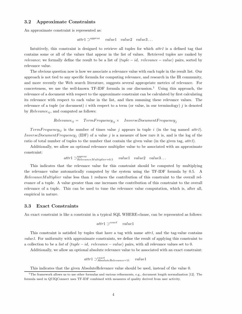
3.2 Approximate Constraints
An approximate constraint is represented as:
attr1 ⊃approx value1 value2 value3 . . .
Intuitively, this constraint is designed to retrieve all tuples for which attr1 is a defined tag that
contains some or all of the values that appear in the list of values. Retrieved tuples are ranked by
relevance; we formally define the result to be a list of 〈tuple − id, relevance − value〉 pairs, sorted by
relevance value.
The obvious question now is how we associate a relevance value with each tuple in the result list. Our
approach is not tied to any specific formula for computing relevance, and research in the IR community,
and more recently the Web search literature, suggests several appropriate metrics of relevance. For
concreteness, we use the well-known TF-IDF formula in our discussion.1 Using this approach, the
relevance of a document with respect to the approximate constraint can be calculated by first calculating
its relevance with respect to each value in the list, and then summing these relevance values. The
relevance of a tuple (or document) i with respect to a term (or value, in our terminology) j is denoted
by Relevanceij , and computed as follows:
Relevanceij = TermFrequencyij × InverseDocumentFrequencyj
TermFrequencyij is the number of times value j appears in tuple i (in the tag named attr1).
InverseDocumentFrequencyj (IDF) of a value j is a measure of how rare it is, and is the log of the
ratio of total number of tuples to the number that contain the given value (in the given tag, attr1).
Additionally, we allow an optional relevance multiplier value to be associated with an approximate
constraint:
attr1 ⊃approxRelevanceMultiplier=0.5 value1 value2 value3 . . .
This indicates that the relevance value for this constraint should be computed by multiplying
the relevance value automatically computed by the system using the TF-IDF formula by 0.5. A
RelevanceMultiplier value less than 1 reduces the contribution of this constraint to the overall rel-
evance of a tuple. A value greater than one increases the contribution of this constraint to the overall
relevance of a tuple. This can be used to tune the relevance value computation, which is, after all,
empirical in nature.
3.3 Exact Constraints
An exact constraint is like a constraint in a typical SQL WHERE-clause, can be represented as follows:
attr1 ⊃exact value1
This constraint is satisfied by tuples that have a tag with name attr1, and the tag-value contains
value1. For uniformity with approximate constraints, we define the result of applying this constraint to
a collection to be a list of 〈tuple− id, relevance− value〉 pairs, with all relevance values set to 0.
Additionally, we allow an optional absolute relevance value to be associated with an exact constraint:
attr1 ⊃exactAbsoluteRelevance=11 value1
This indicates that the given AbsoluteRelevance value should be used, instead of the value 0.1The framework allows us to use other formulas and various refinements, e.g., document length normalization [12]. The
formula used in QUIQConnect uses TF-IDF combined with measures of quality derived from user activity.
4
3.4 Combining Exact and Approximate Constraints
We allow constraints to be composed using the boolean operators AND and OR.
The result of evaluating a constraint is always a list of 〈tuple − id, relevance − value〉 pairs sorted
by relevance-value. For any single constraint, we also know whether it is approximate or exact, and this
is important when combining the results of multiple constraints.
We therefore modify our definition of the result of a single constraint to also include exactly one of
the two properties exact or approximate. For composite query terms (i.e., terms containing ANDs and
ORs) we define the result recursively as follows, in terms of the results of the component constraints,
Constraint1 and Constraint2:
CombinedConstraint ::= Constraint1 AND Constraint2
If the result of either Constraint1 or Constraint2 is marked exact then the result of CombinedConstraint
is defined as follows:
If (a pair containing) a tuple-id appears in the results of both Constraint1 and Constraint2,
then it is in the result of CombinedConstraint, with its relevance equal to the sum of the
relevances of that tuple in Constraint1 and Constraint2. Otherwise, this tuple-id is not in
the result. The result of CombinedConstraint is marked exact if both input constraints are
exact, and approximate if one of them is approximate.
If the results of Constraint1 and Constraint2 are both marked approximate, then the result of
CombinedConstraint is also marked approximate, and is defined as follows:
If a tuple-id appears in the result of either Constraint1 and Constraint2, then it is in the
result of CombinedConstraint. Its relevance is equal to the sum of its relevances in the
results of Constraint1 and Constraint2.
Next, we turn to the OR connective.
CombinedConstraint ::= Constraint1 OR Constraint2
If a tuple-id appears in the results of either Constraint1 or Constraint2, it is in the result of
CombinedConstraint. Its relevance is equal to the sum of its relevances in the results of Constraint1
and Constraint2. The result of CombinedConstraint is marked exact if both input constraints are
exact, and approximate otherwise.
We found it useful to introduce an operator called ModifyRelevance:
CombinedConstraint ::= Constraint1 ModifyRelevanceRelevanceMultiplier=1.2 Constraint2
Here, Constraint1 must be an approximate constraint, and Constraint2 can be either approximate
or exact. The result is identical to the result of Constraint1, with the modification that if a tuple
also appears in the result of Constraint2, its relevance is multiplied by the RelevanceMultiplier value.2
This operator is used to reorder the result of Constraint1 based on the result of Constraint2, without
actually removing or adding any new tuples.
We conclude our presentation of relevance queries with the following observation:
2Actually, we allow more sophisticated formulae for computing the relevance of the tuples in CombinedConstraint.
Of special interest are those formulae in which the increase or decrease in relevance of a tuple actually depends upon the
relevance of that tuple in Constraint2. However, an in-depth discussion of this topic is beyond the scope of this paper.
5
Theorem 3.1 AND and OR are commutative and associative operators.
As a special case, consider a query that can be specified as “query1 AND query2,” where query1
consists of only approximate constraints and query2 consists of only exact constraints. This corresponds
to the traditional approach to mixing text-retrieval and exact-match queries. The first part is used for
relevance retrieval and the second part is used as a filter. Our framework allows such a query to be
re-ordered for efficient execution using the associativity and commutativity properties of the boolean
connectives without changing the semantics of the query. This increases the optimization opportunities
available to us.
3.5 A New Class of Approximate Queries
While the query framework is motivated by a desire to synthesize capabilities from databases and text-
retrieval, it also offers a powerful new class of approximate queries that go beyond either existing query
paradigm. Relevance-ranking, while most commonly seen in similarity queries over text, is not limited
to text.
For example, suppose that we are searching for “inexpensive cars that are fairly new.” There are two
constraints, on cost and on age. Both constraints are approximate; one suggests returning cars in order
of increasing cost, and the other suggests returning cars in order of increasing age. Given a collection
of cars of varying ages and prices, how do we rank them in response to this query? Intuitively, do we
give more importance to a car being less expensive or to a car being newer? If we take into account the
number of cars that are more expensive than a given car, or that are older than a given car, and use
these numbers to associate relevance with the two (approximate) constraints in this query, we have an
elegant solution to the problem.
The approach that we propose thus generalizes the relevance-ranking principles used in IR systems to
such scenarios in a natural way; statistical properties of cost and age distributions are used to determine
how much importance to give to these two criteria.
Further, we can freely intermix conventional database-style (exact) constraints with approximate
criteria. For example, suppose that we are searching for “inexpensive cars under 5 years old”. The
second constraint, interpreted as an exact constraint, eliminates cars under 5 years of age, and we expect
to see qualifying cars in order of increasing cost. This is precisely what our relevance framework achieves.
Handling such queries, however, requires us to examine the semantics of ordered domains (e.g., the
domains of values for age and cost) in a particular manner. This leads to implementation challenges
that go beyond the scope of this paper.
4 Implementation of a Unified Retrieval System
Arguably, the biggest differences between DBMSs and IR systems stem from their workload. A DBMS
must provide transactional support for update workloads, and has concurrency control and recovery
mechanisms. An IR system can consider query-only workloads, with periodic index rebuilds, and can
build highly optimized index structures without regard to dynamic maintenance. In our hybrid system,
text plays a dominant role and must be indexed as in an IR system, but updates are frequent, and
periodic offline refreshes are unsatisfactory.
Typically, applications that need to incorporate both text data with other data in their searches end
up indexing the text portion of the data using an Information Retrieval search engine, and the other
data using a completely independent database engine. Input queries are broken up into two parts: a
6
text-search portion, and an exact-match portion. These queries are sent to the two independent search
engines and the results are merged together. This approach has limitations in terms of performance
because selective constraints that go to one of the two component engines cannot be used to effectively
prune the computation in the other engine. It also does not support the range of queries that we aim to
support. For example, we cannot express the example “inexpensive car under 5 years” query.
In our hybrid approach, text and non-text data can be combined in a single index. This allows
us to have a very sophisticated algorithm for computing relevance of a tuple to a given query, in turn
enabling us to support queries such as the example car query. It also allows relevance computation to
be controlled extensively by means of query constraints, and allows optimizations in query processing
that are not easy to achieve otherwise.
The design and performance objectives that we seek to achieve are:
• The system must support (near) real-time indexing.
• It must be recoverable. That is, in case of crashes due to software or hardware problems, when
the server is restarted it recovers from the crash and puts the index in a state consistent with the
production database without losing any data.
• It must be efficiently recoverable. That is, recovery after a crash must be very fast; a complete
index re-build is unacceptable.
• It must be self-reorganizing. The system should automatically re-organizes the index structures
periodically for maximum efficiency without incurring any downtime for re-organization.
• Concurrency with consistency. The system must allow concurrent access for reading as well as
inserting/updating data without leading to loss or corruption of data.
4.1 Non-Text Data Types
Traditional databases contain values of traditional data-types like integer, floating point number, date,
or string, or its value can be a text document. We now describe how these different data-types can be
indexed using the scheme we have described so far.
The basic idea is to map non-text data to pseudo-keywords in our system. Specifically, we set aside
a fixed number N (for example N might be 100,000) pseudo-keywords for this purpose. We give them
values that cannot be confused with actual keywords of text data. Then, we associate a distinct integer
value between 1 to N with each pseudo-keyword. Now, each distinct value that a non-text attribute in
the database might take is mapped to one or more of the pseudo keywords. The mapping scheme can
differ based on the datatype of the attribute. For any data-type whose domain has less than N distinct
values, we map each distinct value of that domain to a value from 1 to N, and use the corresponding
pseudo-keyword as the “keyword value” of that value. For data-types whose domain does have more
than N distinct values, we use some hashing scheme to map each distinct value in the domain to some
integer from 1 to N. Multiple values in the domain can map to the same integer value. However, with
the choice of a good hash function, such “collisions” can be minimized. Some post-processing is needed
to remove the false positives from the results; we omit the details.
This mapping scheme allows us to regard every attribute in every tuple in the database as a collection
of keywords or pseudo-keywords. Thus, all queries over this data can be expressed as keyword queries.
7
5 System Architecture
The architecture of QQE consists of a DBMS that holds all the base data and an external index server
that maintains the unified index. Inserts/Updates are made directly to the base data in the DBMS.
Whenever such an update is made, a log record is written to the JOBS table in the DBMS as a part of
the same transaction. This record gives logical details of the change that was made to the base data. All
records in the JOBS table are stamped with the time when the record was inserted. A reader process
periodically polls the JOBS table and fetches the latest records and submits them to one or more index
server processes. The index server processes apply the modifications to the dynamic index in the order
they jobs are received.
The JOBS table serves as a redo log and is used for crash-recovery. It also simplifies the index server
update processing by serializing all the transactions.
5.1 Overview of Our Approach to Deferring Updates
Our basic idea is to defer applying update operations to the persistent store. Updates are handled in
three steps: (1) Changes to the database are reflected in a special table. (2) The changes are continually
polled and incorporated into a differential index structure. (3) The main index is periodically refreshed
to absorb the differential index. These details must be transparent to data retrieval operations, and
therefore retrieval operations have an additional step of checking results against the differential index to
adjust for changes that have not yet made it to the main index.
This approach allows us to disregard random updates and optimize persistent index structures as
if they were static, since they are refreshed offline and accessed sequentially. Since query processing
time is dominated by processing constraints to identify the top results, these index optimizations can
dramatically improve performance. Periodic refreshes can also be combined with analysis/mining of
query and update traces to make the system self-tuning at the storage level, extending the current state
of the art (in which automatic tuning has largely been limited to the choice of indexes).
5.2 Data Structures
The primary data structure in QQE is an inverted index, or reverse mapping, that maps each token
appearing in an attribute to a TIDLIST. Each entry of the TIDLIST is a TID and a count that represents
the number of times the token appears in the given attribute of the TID’s tuple. Entries are sorted in
descending TID order, i.e., youngest tuples first, and an entry does not appear for counts of zero token
occurrences. Other important data structures are the concept table and log. Since many of the tokens
come from attributes that are often unstructured and contain the expected ambiguities associated with
natural language, the concept table maps a concept to a set of tokens, and provides a mechanism to
alleviate such ambiguities; we will not discuss it further in this paper. In order for the inverted index
and the concept table to be recoverable, modifications to either are first written to a log before being
applied to either data structure.
There are many options for how to manage the inverted index. The design is based on the assumption
that the number of changes will be small relative to the number of queries. Furthermore, it is critical that
query response times be fast. As a result, the inverted index is maintained both on disk and in memory.
The disk version, referred to as the static index, is partitioned into N read-only partitions. A token is
hashed into one of N partitions which stores a linear probe hashtable whose associated TIDLISTs are
tightly packed in order to maximaze I/O bandwidth. Since an insert operation may require an entry
to be inserted into the middle of a TIDLIST, modifications are deferred into the in-memory version, or
8
dynamic index. Periodically, the two versions are synchronized, or merged on a partition-by-partition
basis. Corresponding partitions from the static and dynamic indexes are merged and the result is written
out to a new location on disk. Partitioning the index reduces the contention for resources during merging
and avoiding in-place writes greatly simplifies concurrency control and decreases query response times.
Cycling through all partitions effectively rewrites the entire static index.
Within each partition, we have a two-level index. First, there is a hash-table or a tree structure that
maps a value to a value-hashtable. Given any (tokenized) value, this table allows us to find the value-
hashtable. The value-hashtable is a second-level hashtable that contains all the entries corresponding to
the occurrence of this value in all the tables/attributes in the database. The value-hashtable is keyed
off the composite key Collection+Tagname and stores a TIDLIST.
We also break each Partition into two parts. One part consists of old data that resides exclusively on
the disk, and another part consists of new data that resides exclusively in the main memory of the index
server process. Specifically, all updates, inserts, and deletes that happened after some point in time T
are considered new and are stored in the in-memory portion of the Partition. All data older than T are
considered old and are stored on the disk portion of Partition.
All new updates to this Partition are done only to the in-memory portion. The on-disk portion of
the Partition is not updated at all. Queries over this partition are evaluated by merging the results from
the on-disk index and the in-memory index. Periodically (for example, once per day), the on-disk and
in-memory portions are merged and a brand new merged index is written out to the disk. Now in an
atomic operation, the old on-disk index for this Partition is deleted and replaced by the new merged
index AND the in-memory index is deleted and replaced by and empty in-memory index.
5.3 Process Structure
A reader process submits modifications to a pool of server processes. The job of the reader process
is to ensure that all servers receive all the modifications from the JOBS table in the correct order (by
timestamp) and in a timely fashion.
Whenever a server re-starts after a crash, it reads all the disk-files that hold the index partitions.
Each partition i has an associated timestamp Ti indicating the most recent job reflected in the on-disk
portion of this index partition. At start-up, or during crash-recovery, the server sends the the timestamp
of the oldest partition (that is, the min(Ti)) to the reader and requests it to send all jobs with a newer
timestamp. After this point, the reader keeps feeding the servers with the appropriate jobs from the
jobs table. For each server it keeps track of the timestamp of the most recent job that has been sent
successfully to that server. Periodically, it scans the JOBS table to check if there are any jobs in the
JOBS table with a timestamp newer than the timestamp of any of the servers, and sends those jobs to
the appropriate servers. Note that due to this protocol there is a delay beween inserting a tuple into
QUIQConnect and being able to query it using QQE. Currently the delay is 30 seconds. Recovery, which
is discussed in Section 8 follows directly from this protocol between reader and server processes.
We discuss servers in more detail next.
6 The Server
The server process maintains the inverted index in order to answer queries. Each modification request is
first applied to the dynamic index. The dynamic index in a partition is merged with the corresponding
static index periodically in a staggered fashion. Currently, the system cycles through all partitions within
a day. In addition, when a large number of modifications needs to be applied to the index, the server
9
can be operated in a bulkload mode. The following subsections describe in greater detail how the data
structures are used for the primary operations of updating, querying, merging, and bulkloading.
6.1 Handling Changes
The changes to the index that are handled by the server are inserting a tuple, updating a tuple’s attribute
value, and deleting a tuple. We also support an append operation wherein new text is appended to the
existing value of a given attribute of a tuple. The modifications to the concept table are not covered as
they follow from the operation described on the inverted index.
An insert modification request is represented as <TID, Collection{( attr1,tokens), attr2,tokens),
...(attrN,tokens)} >. The server translates the request into the following TIDLIST look-ups in the
dynamic index:
1. <Collection,attr1, token1-1>
2. <Collection,attr1, token1-2>
3. <Collection,attr2, token2-1>
4. <Collection,attr2, token2-2>
5. <Collection,attrN, tokenN-1>
6. <Collection,attrN, tokenN-2>
If no TIDLIST is found a new TIDLIST is created. If the TID exists in the TIDLIST, its count is
incremented, otherwise, a new entry for the TID with a count of 1 is inserted.
As far as the index structure is concerned, an append operation is identical to an insert operation.
The delete operation is handled by maintaining a bitvector that records if a tuple is deleted or not.
Queries use the bitvector to mask out those tuples that satisfy the query but have been deleted. The
bitvector is also used during the merge process to skip writing out entries of TIDLISTs whose tuples
have been deleted.
The update operation is the least straightforward of the operations. If the given tuple has not been
updated recently, there will be no information about this tuple in the dynamic index. Here, the update
is treated as an insert. The new tokens associated with this tuple are simply inserted into the dynamic
index. In addition, an ignore-disk bitmap is maintained which indicates that all the information in the
static index relating to this TID should be ignored during query processing.
This scheme runs into problems if the tuple has been updated recently and hence there are entries
associated with this TID in the dynamic index. In that case just inserting the new value of this tuple
into the dynamic index is not good enough because that will result in current values in the dynamic
index being merged with the new values. In order to process such an update, the old attribute value
is compared against the new value. Tokens added are processed as an insert into the dynamic index
and removed tokens require the TIDLIST entry for the tuple to be decremented3. It is very difficult to
retrieve the old value of a tuple in an inverted list index structure. That would require a full scan of the
entire index. Since this is expensive, a data structure is maintained in memory called a forward map
that stores the current values of those tuples which are currently present in the dynamic index.
Even though the forward map only holds information about tuples that are present in the dynamic
index (i.e., tuples that have been updated/inserted recently), it is still an inefficient use of main memory.
3Only the TIDLIST entry in the dynamic index needs to be decremented. We don’t have to make any changes to the
static index. That is still handled using the ignore-disk bitmap.
10
It essentially doubles our memory requirement. Such a forward map can be avoided if the application
can include the old value of a tuple with each update request that is sent to QQE server.
6.2 Answering Queries
The types of queries handled by the server are described in Section 2. While Section 7 describes the
algorithms used for query processing, this section focuses on how the index data structures are used to
evaluate a query. For this purpose, it is sufficient to treat a query as a set of contains constraints of
the form: {attr0 CONTAINS token0, ..., attrM CONTAINS tokenN }. For each CONTAINS constraint,
the inverted index is probed to retrieve the corresponding TIDLIST. In order to get the most up-to-
date data, the contents of the dynamic and static indexes are merged. This merge operation is a little
complicated since it has to take into account the ignore-disk bitmap described in the previous section.
Essentially, a merge uses the following formula:
result-tidlist = merge3 (static-tidlist, dynamic-tidlist, ignore-disk)
Here, the merge3 operation is implemented as follows:
result-tidlist[TID] = dynamic-tidlist[TID] if ignore-disk[ TID] is TRUE
= static-tidlist[TID] + dynamic-tidlist[TID] if ignore-disk[TID] is FALSE
In other words, use only the values from the dynamic index if ignore-disk is true, otherwise add the
values together. Finally, all deleted tuples are masked out from the combined TIDLIST using the delete
vector.
result-tidlist = result-tidlist - deleted-tids
6.3 Merging Dynamic and Static Indexes
Periodically, QQE refreshes the static index by merging it with the dynamic index and writing a new
static index. Merging is done one partition at a time and each partition can be merged independently
of other partitions. Using this organization, the entire static index is merged over the period of a day
by staggering the partition merges. When a partition is merged, changes are disallowed to the dynamic
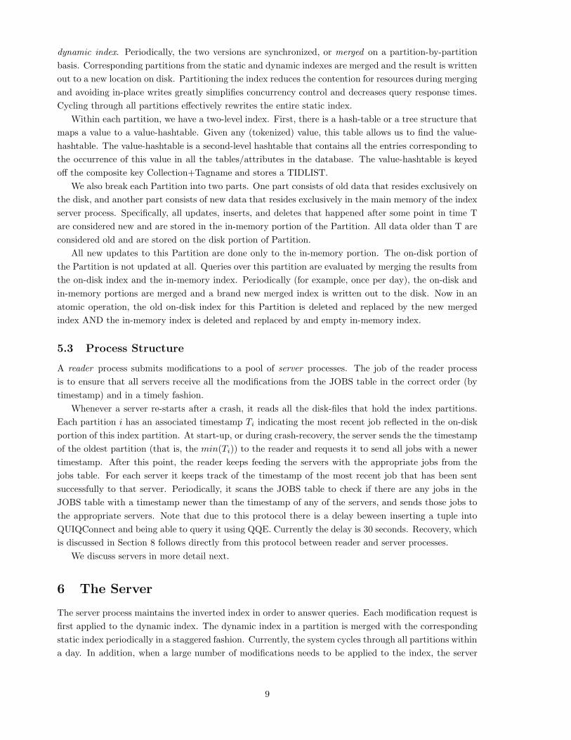
partition while it is being merged with the static partition. In order to handle change requests, a new
dynamic partition is constructed and change requests that arrive during the merge are applied to this
new partition. As a result, answering queries is slightly complicated by now having to consider three
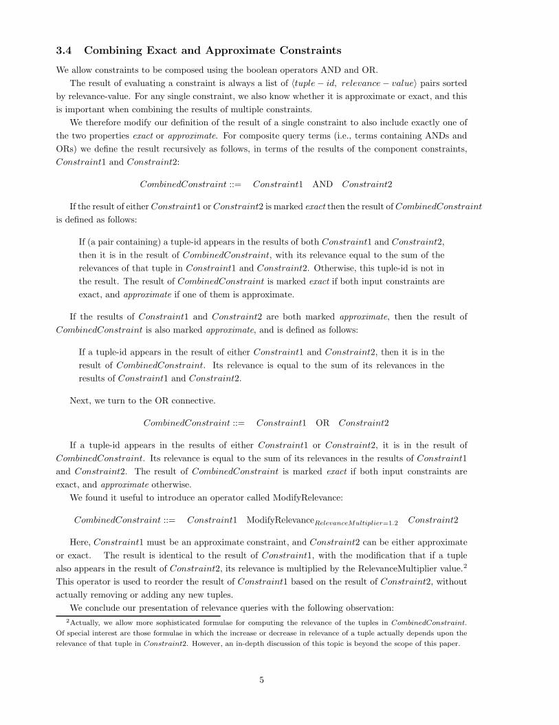
structure: the new dynamic partition, the frozen dynamic partition, and the static partition. Figure 1
illustrates all of the data structures during the merging of a partition. Section 8 covers in greater detail
the steps taken to insure that the refresh procedure allows a high rate of concurrent readers and writers.
Some beneficial properties arise from being self-organizing as a result of continually rewriting the
index. First, queries are fast since the organization of the index on disk does not have to account for
free-space often required of systems that apply changes in-place. A further speed-up is due to reduced
locking contention. However there is a tradeoff: system resources are spent writing all of the index
whereas some parts of the index are rarely modified.
A further benefit is that related data such as statistics are regularly refreshed as a side-effect. For
example, the number of entries in a token’s TIDLIST represents the number of times a token appears in
an attribute and is used in query evaluation as discussed in Section 7. Because of deletes, the TIDLIST
length is not accurate and is expensive to correct for every token. However, since the index is continually
refreshed and given that the rate of change is uniform and low in volume, the error in the statistic is
expected not to deviate significantly from the true value and is used without correction.
11
N0 i
Log0 N
QQE ServerQQE Reader
Cchanges
Archiving
i
Queries
Client
Figure 1: A Snapshot of QQE as Partition i is
Merged.
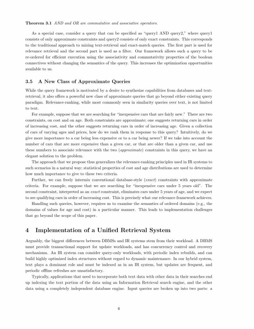
Header Body Category IsExpert
And Or
IsExpired
And−Not
fantasy
football
realconcept−0
Body
soccer
Filtertrue
QualityFilter
Match
Figure 2: The Plan for the Example Query
A final benefit of a self-organizing index is in evolution flexibility. For example, format changes may
be incorporated by simply restarting the server process with the new version of the executable to read
and write the new format.
6.4 Bulkload
The mode of the server that is optimized for loading large amounts of data is referred to as bulkload. The
motivation for bulkload is to efficiently handle large sets of scheduled change requests, such as during
an initial seeding from a migration or during a recovery from media failure. The server procedures for
handling changes are inefficient for large volumes of data. First, the forward-map must be maintained;
and second, when memory is fully consumed, the only way to make progress is to merge the dynamic
index with the static index. Such a merge requires all partitions to be written and is very expensive. A
large number of inserts/updates might require the entire index be merged multiple times, resulting in
very poor results. The bulkloading algorithm attacks this issue through a partitioned approach.
The Partitioned Bulkload algorithm proceeds in two phases. The first phase is the partitioning phase.
A change request may span multiple partitions, and so all change requests for tuples are partitioned
according to which static partition they affect. How to partition a single tuple modification is determined
using the same hash function as used at query time. Each partition’s changes are written out to separate
files. The second phase is the update phase. Each partition’s set of changes is read in and applied to
a single partition using the same procedure as a normal update. After the updates of a given partition
are processed, the corresponding partition index is refreshed (i.e., the dynamic index and static index
of that partition are merged and written out to disk, creating a new static index). This frees up all the
main memory that was used by this partition. The algorithm saves an order of magnitude in processing
time as compared to using the standard update algorithms. Note that while the server is bulkloading
the index, it can still process queries over the old data.
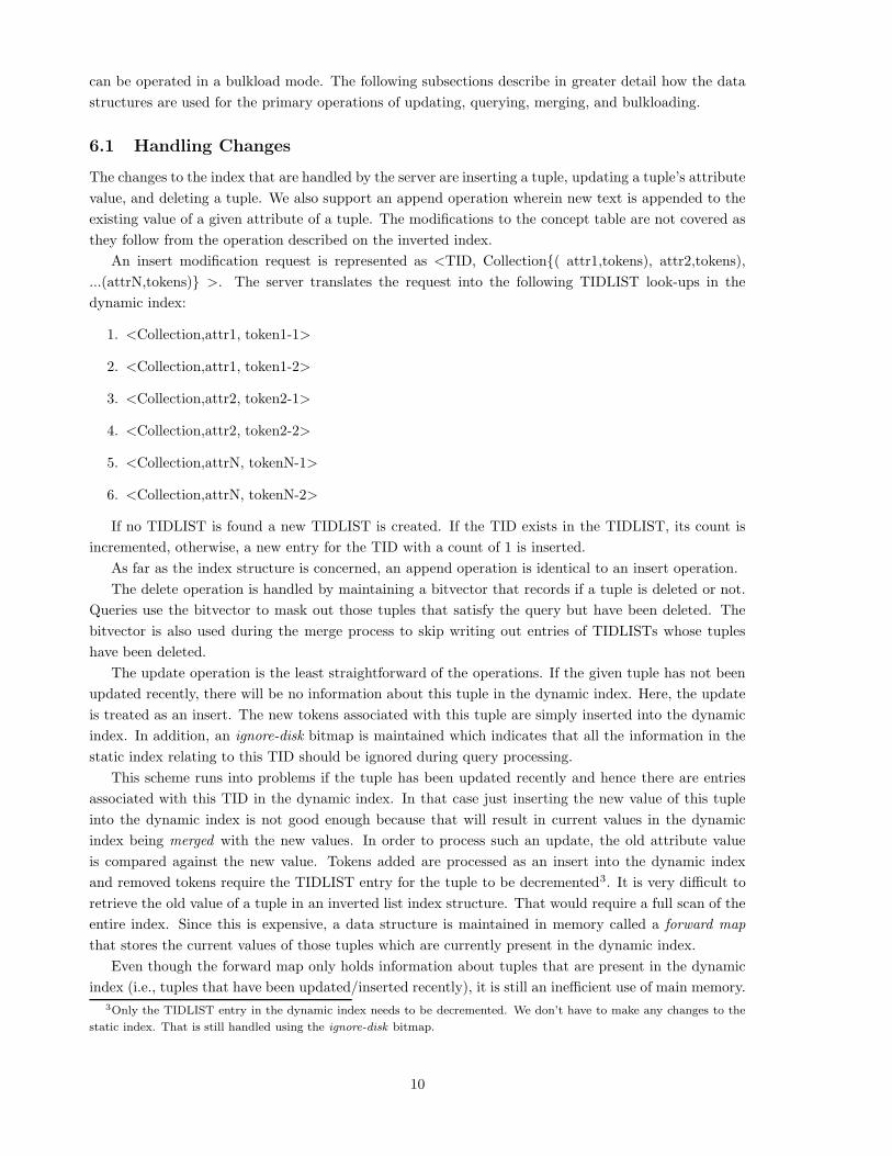
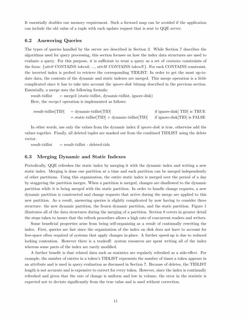
7 Query Processing
A plan for the example match–filter–quality query from Section 3 is shown in Figure 2. Note that
the same tokenization is applied to a query as is applied to the data. In the example, stopwords and
punctuation are removed, and, although it is not apparent in the example, stemming is typically applied
as well. The constraints are partitioned into positive or negative. The order of constraints in the plan
12
determines the evaluation order. Positive constraints with match are evaluated first, then filter and
quality constraints, and finally the negative constraints. The match constraints are approximate, and
therefore expand the result set. The filter constraint can only reduce the result set whereas the quality
constraint can reorder the result set. The negative constraints can only reduce the size of the result set.
If an OR of such queries is received, evaluation proceeds independently on each side of the OR and the
result sets are unioned.
During query evaluation, the constraints may be re-ordered to reduce the amount of computation.
For example, a filter constraint that is very selective can be evaluated before the other constraints thus
setting an upper limit on the size of the results. This would in keeping the computation costs low for the
rest of the query evaluation. The query semantics are such that all quality constraints must always be
applied after the filter and match constraints. However, filter and match constraints that are connected
by AND operators can be freely re-ordered without changing the meaning of the query.
7.1 Optimization
Since query evaluation can be resource intensive, certain optimizations are included in the plan. Par-
ticularly, query evaluation becomes more expensive as the total size of the TIDLISTs increases which
is influenced by the number of tokens and the individual TIDLIST sizes of the tokens in the query. As
a result, the optimizations only apply to the evaluation of the match constraints. One class of opti-
mizations focuses on dropping tokens. The tokens dropped are the ones that have the least IDF value
associated with them. In other words, these are tokens which are likely to contribute the least to the
relevance value of a result tuple. An added bonus is the fact that the least relevant tokens also tend to
have the longest TIDLISTs associated with them. Another optimization limits how much of a TIDLIST
to read in. Since TIDLISTs are stored in descending TID order, this optimization gives lower priority
is to older tuples. Finally, the size of the result set can be optimized against. Given a target result
set size, TIDLISTs are evaluated until the limit is reached after which point, the remaining tokens only
update the relevance values in the current result-set as opposed to adding new tuples to the result set.
All of the optimizations can be combined and the selection of an optimization is statically chosen by an
administrator.
8 Concurrency and Recovery
Concurrency during normal processing, i.e., in the absence of merging, requires only short term latches
since the disk structures are never written. During merge, the situation is more complicated. In order
to allow modifications to be applied during a merge, the dynamic index is frozen and a new dynamic
index is created. While the frozen dynamic index partition is merged with the static index partition and
written to a new file, change requests can applied to the new dynamic partition. In addition, queries
now have to consider three structures from which to merge results: new dynamic, frozen dynamic, and
static index. When the new parition is written to disk, a file pointer is swapped and the frozen dynamic
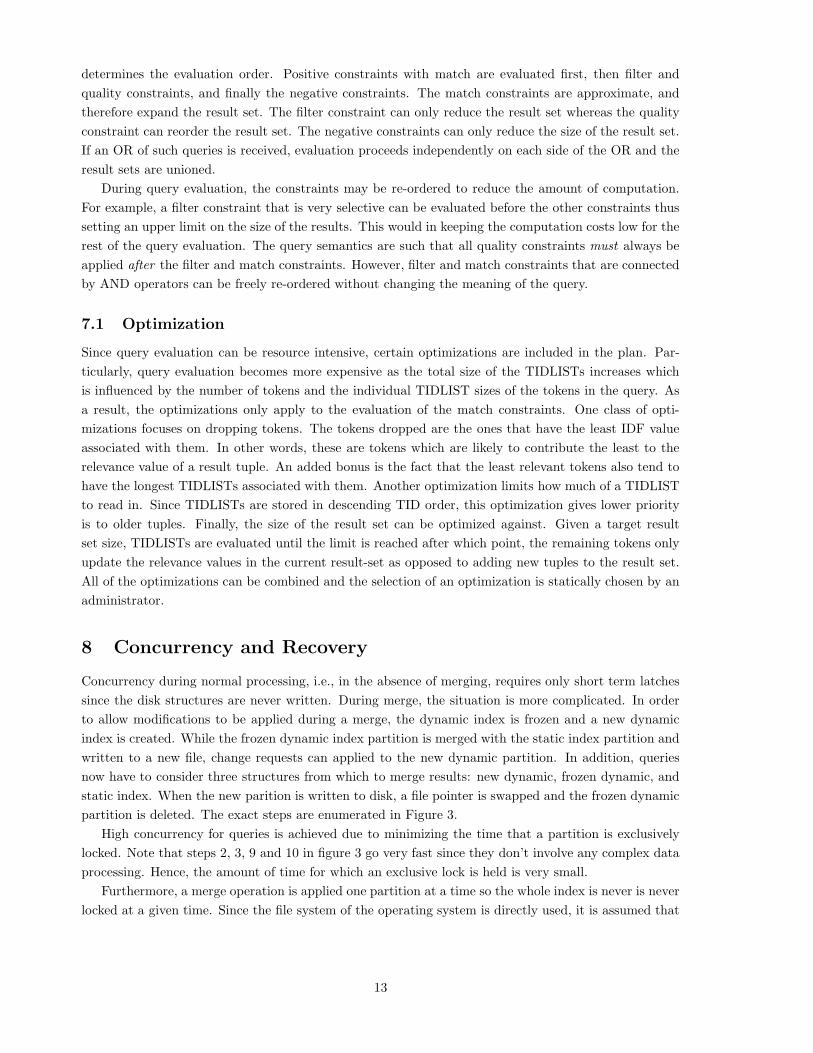
partition is deleted. The exact steps are enumerated in Figure 3.
High concurrency for queries is achieved due to minimizing the time that a partition is exclusively
locked. Note that steps 2, 3, 9 and 10 in figure 3 go very fast since they don’t involve any complex data
processing. Hence, the amount of time for which an exclusive lock is held is very small.
Furthermore, a merge operation is applied one partition at a time so the whole index is never is never
locked at a given time. Since the file system of the operating system is directly used, it is assumed that
13
1. Exclusively lock partition i, disable updates
2. Mark dynamic partition Di as frozen and create a new dynamic partition for i, D′
i
3. Record the timestamp of the last modification applied to Di
4. Release the lock on i
5. Merge Di with static partition i, Si
6. Write the merged data structure to a new static partition S ′
i
7. Record in S′
i the timestamp from step 3
8. Exclusively lock partition i
9. Delete Si
10. Rename S′
i to Si
11. Release the lock on partition i, enable updates
12. Delete Di
Figure 3: Steps Required to Merge a Partition
a reader thread can continue reading the orginally openned file while a merger thread renames the newly
written partition to the existing partition.
Recovery proceeds by using the minimum of all of the partition timestamps written in step 7. The
minimum timestamp is given to the reader process that processes the log, as described in Section 5.3.
Except for the brief period when the partition is exclusively locked, queries, inserts and deletes can
proceed concurrently with the partition merge process. Unfortunately, this is not true of updates. Due to
the semantics of the ignore-disk bitmap, an update cannot be run concurrently with the merge process.
If different portions of a single update transaction touch the ignore-disk bitmap of a partition before
and after the partition is merged, this will result in a loss of data. Due to this all updates that touch a
given partition have to be blocked while a partition merge process is in progress.
Currently, inserts, updates and deletes are all handled by a single thread in a server, and are processed
in the order they are received. When an update blocks because a partition merge is in progress, the
entire thread blocks, resulting in a blockage of any inserts/deletes that follow. This thread remains
blocked until the partition merge finishes. Since insert-tuple and delete-tuple cannot really interfere
with update-tuple jobs, it is possible to let insert-tuple and delete-tuple jobs to proceed even though an
update is blocked. However, this optimization has not currently been implemented in our system. As a
consequence, inserts and deletes in the system can proceed concurrently with a partition merge, but all
changes will stop at the first update that touches that partition.
Several properties hold with respect to our concurrency and recovery protocols. Let us call the system
quiescent if no inserts/updates/deletes are in progress, no partition is currently being merged, and no
queries are currently being processed; and active otherwise.
Theorem 8.1 1. In a quiescent system, the logical state of the index is identical to what it would
have been if all the jobs in the JOBS table had been applied to the index sequentially, in the absence
of queries and merge activity.
14
2. A query run on a quiescent system will always see all the data from all the update/insert/delete
jobs that have completed.
3. A query run on an active system will see all the change made by update/insert/delete jobs that are
complete at that instant. In addition (unfortunately), it might see partial data from the job that is
in progress at that instant.
4. Merge activity (whether in progress or completed) does not alter the logical state of the index. In
the absence of concurrent insert/delete/update jobs, a query that is run before, during or after
one or more partitions are merged will produce exactly the same results. Any sequence of in-
sert/delete/update jobs that run during a merge process results in the same logical state of the
index as obtained if those jobs ran in the absence of merge activity.
Theorem 8.2 1. Each partition i has an associated timestamp Ti. This indicates that the on-disk
portion of partition i reflects all the jobs in the JOBS table with timestamp ≤ Ti. During recovery
from a crash, a job is applied to a partition i if and only if its timestamp is greater than Ti.
2. After recovery is complete, the logical state of the index is the same as it would have been if all the
jobs had been applied sequentially to the index in the absence of any crashes, partition merging,
and queries.
3. If we ensure that the in-memory portion of all partitions are merged with the respective on-disk
index at least once per day, then it is never necessary to fetch jobs older than one day during the
recovery process (except in the case of media failure).
To recover from media failure, we simply restore the disk files from a backup, and restart the server.
The crash-recovery process will take care of the recovery after this point. The system automatically
figures out the smallest Ti associated with the oldest partition from the backups and fetches jobs newer
than that. The rest of recovery is exactly as described before.
9 Performance
In this section, we present results from a performance study of QQE. Specifically, we measure how
effectively the system can handle workloads composed of only queries, only inserts, only updates, as well
as a mix of queries and changes. In addition, we study bulkloading algorithms as well as the effect of
merging static and dynamic indexes on queries. As a part of the study, we implement the functionality
of QQE using an alternative system to which we apply the same workload. All experiments are run on
Pentium III dual processor machines with 1GB of memory, disks with a SCSI disk interface, and the
Linux operating system kernel version 2.4.18.
9.1 Studying QQE Standalone Performance
9.1.1 Queries
In this section we study the performance of queries in the system. The database consists of about 240,000
tuples, with an average size of about 3200 bytes per tuple. Specifically, there is a Header field in each
tuple that has average size of 160 bytes, and an Body field that has an average size of 1320 bytes. The
important parameters that affect query performance are the number of tokens (keywords) in the query,
the frequency of the tokens in the database, and the average size of the attribute being queried.
15

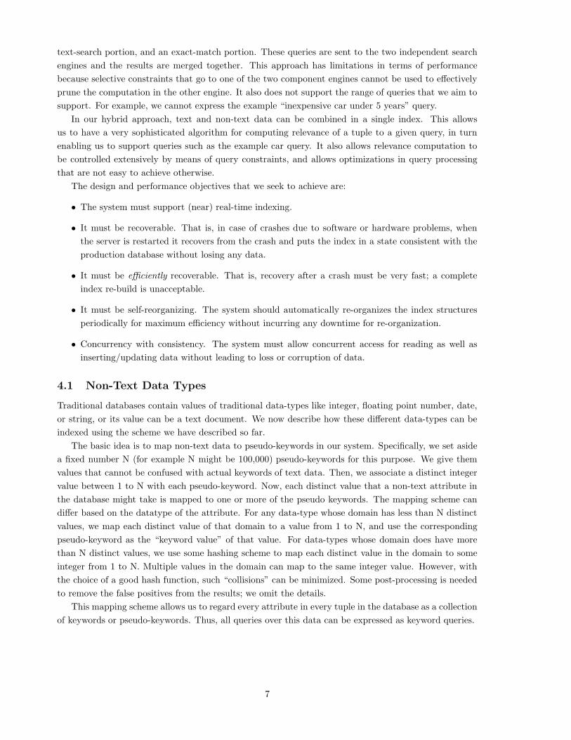
406080
100120140160180200220240
2 4 6 8 10 12 14 16 18 20
Tim
e (s
ecs)
Number of tokens
Low FrequencyHigh Frequency
Figure 4: Queries on the Body Field
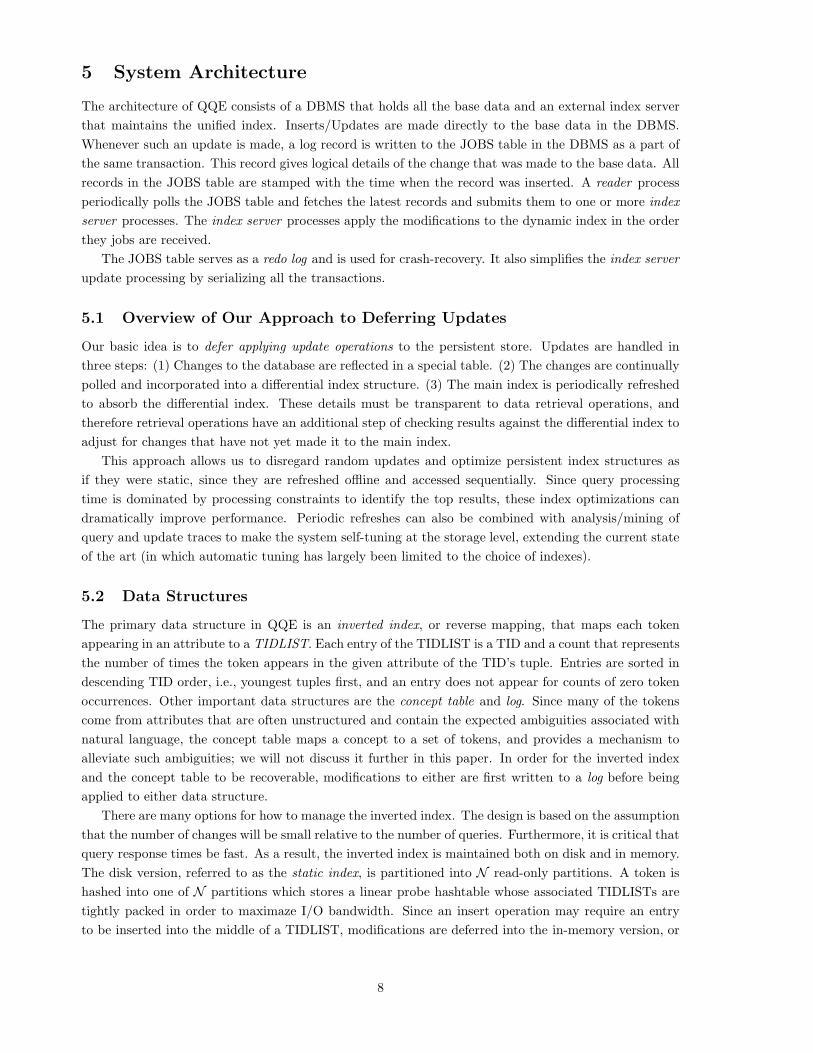
0
200
400
600
800
1000
1200
1400
1600
1800
20
Tim
e (s
ecs)
Number of tokens
LimitResultsDropTokens
DropTokensWithCache
Figure 5: Effect of Optimizations
Figure 4 shows the results of time taken to run the query workload as the number of tokens in the
query was increased upto 20. We note that the time taken shows a slightly super-linear increase as the
number of tokens is increased. This is to be expected, since the amount of work done for evaluating a
query is directly proportional to the number of tidlists that have to be fetched and processed. The super-
linear behavior is because of the fact that as the number of tokens increases, the size of the resultant
tidlists begins to grow, and the cost of merging the tidlists increases.
For this experiment, we chose a set of tokens each of which appears in more than 2% of all the
tuples in the system. These are the high frequency tokens. We chose another set of tokens each of
which appears in less than 0.2% of the tuples. These are the low frequency tokens. For each experiment,
queries were constructed by choosing N random tokens from the appropriate token set (high frequency
or low frequency) looking up the appropriate field (Header or Body). N was varied from 1 to 20. For
each value of N , 10 different clients each executed 100 such random queries. Evaluation of each query
consists of three steps. First, the entire query results were evaluated in the index server. Then the top
ten TIDs were fetched from the index server. Finally, these 10 tuples were fetched from the RDBMS.
We note that in all these experiments, the last two steps represent a fixed cost. The only thing that
usually varies from experiment to experiment is the cost of evaluating the query in the index server.
As the number of tokens in a query increases, the time taken increases rapidly. The increase is in
fact super-linear. This is because in addition to the cost of retreiving the TIDLISTs associated with
each token, the query has to merge the TIDLISTs. Since the merge is essentially an OR operation, the
sizes of the TIDLISTs to be merged increase with each extra token. Increasing the number of tokens
not only increases the number of fetch-TIDLIST and merge-TIDLIST operations, but also increases the
size of each merge-TIDLIST operation. Hence the performance deteriorates rapidly. Figure 5 shows the
effect of the optimizations for large queries discussed in Section 7.1. The optimizations considered were
DropTokens (in which only the top 20 most relevant tokens were retained in the query, and the others
were dropped), and LimitResults (in which the maximum result set size was set to 10000, and after this
point).
One problem we noticed with the DropTokens optimization was that before the optimization could
be applied, we have to figure out the IDF values of all the tokens in the query. Normally, this requires a
disk access per token (because we need to find the length of the TIDLIST associated with that token).
To reduce this expense, we maintain a cache of IDF values of the tokens in the system. The cache size if
16
limited to 2 MB, and an LRU replacement is used. The result of this experiment (DropTokensWithCache)
is also shown in the figure.
80
90
100
110
120
130
140
150
160
100 200 300 400 500 600 700
Tim
e (s
ecs)
Number of tuples (thousands)
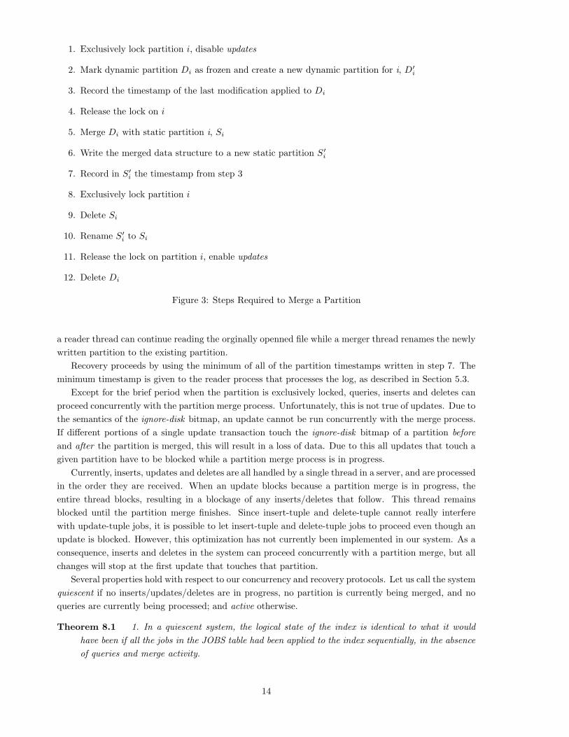
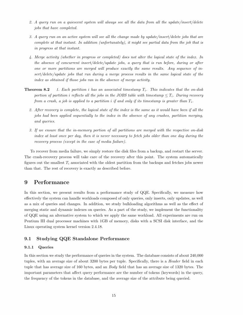
Figure 6: Effect of # of Tuples on Query Perfor-
mance
100
110
120
130
140
150
160
170
1000 2000 3000 4000 5000 6000 7000 8000 900010000
Tim
e (s
ecs)
Avg. Size of tuple (bytes)
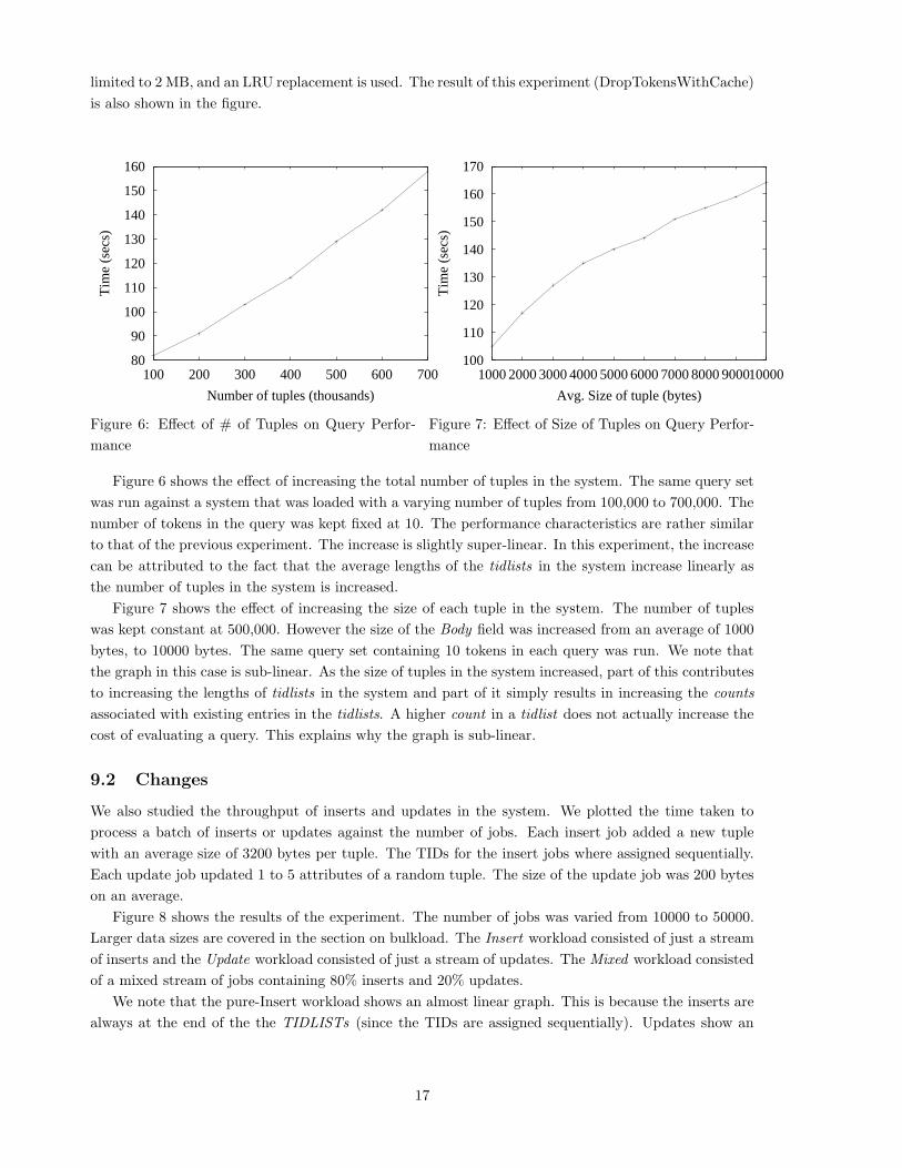
Figure 7: Effect of Size of Tuples on Query Perfor-
mance
Figure 6 shows the effect of increasing the total number of tuples in the system. The same query set
was run against a system that was loaded with a varying number of tuples from 100,000 to 700,000. The
number of tokens in the query was kept fixed at 10. The performance characteristics are rather similar
to that of the previous experiment. The increase is slightly super-linear. In this experiment, the increase
can be attributed to the fact that the average lengths of the tidlists in the system increase linearly as
the number of tuples in the system is increased.
Figure 7 shows the effect of increasing the size of each tuple in the system. The number of tuples
was kept constant at 500,000. However the size of the Body field was increased from an average of 1000
bytes, to 10000 bytes. The same query set containing 10 tokens in each query was run. We note that
the graph in this case is sub-linear. As the size of tuples in the system increased, part of this contributes
to increasing the lengths of tidlists in the system and part of it simply results in increasing the counts
associated with existing entries in the tidlists. A higher count in a tidlist does not actually increase the
cost of evaluating a query. This explains why the graph is sub-linear.
9.2 Changes
We also studied the throughput of inserts and updates in the system. We plotted the time taken to
process a batch of inserts or updates against the number of jobs. Each insert job added a new tuple
with an average size of 3200 bytes per tuple. The TIDs for the insert jobs where assigned sequentially.
Each update job updated 1 to 5 attributes of a random tuple. The size of the update job was 200 bytes
on an average.
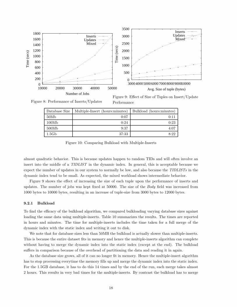
Figure 8 shows the results of the experiment. The number of jobs was varied from 10000 to 50000.
Larger data sizes are covered in the section on bulkload. The Insert workload consisted of just a stream
of inserts and the Update workload consisted of just a stream of updates. The Mixed workload consisted
of a mixed stream of jobs containing 80% inserts and 20% updates.
We note that the pure-Insert workload shows an almost linear graph. This is because the inserts are
always at the end of the the TIDLISTs (since the TIDs are assigned sequentially). Updates show an
17
0
200
400
600
800
1000
1200
1400
1600
1800
10000 20000 30000 40000 50000
Tim
e (s
ecs)
Number of Jobs
InsertsUpdates
Mixed
Figure 8: Performance of Inserts/Updates
0
500
1000
1500
2000
2500
3000
3500
300040005000600070008000900010000
Tim
e (s
ecs)
Avg. Size of tuple (bytes)
InsertsUpdates
Mixed
Figure 9: Effect of Size of Tuples on Insert/Update
Performance
Database Size Multiple-Insert (hours:minutes) Bulkload (hours:minutes)
50Mb 0:07 0:11
100Mb 0:24 0:23
500Mb 9:37 4:07
1.5Gb 37:33 8:22
Figure 10: Comparing Bulkload with Multiple-Inserts
almost quadratic behavior. This is because updates happen to random TIDs and will often involve an
insert into the middle of a TIDLIST in the dynamic index. In general, this is acceptable because we
expect the number of updates in our system to normally be low, and also because the TIDLISTs in the
dynamic index tend to be small. As expected, the mixed workload shows intermediate behavior.
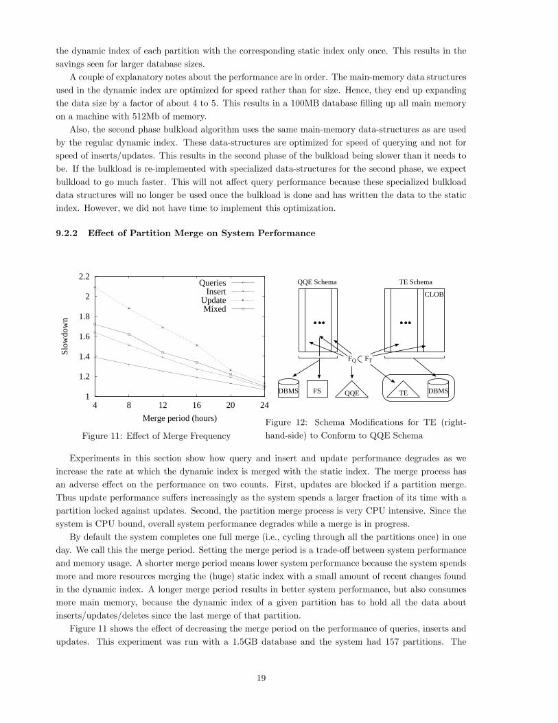
Figure 9 shows the effect of increasing the size of each tuple upon the performance of inserts and
updates. The number of jobs was kept fixed at 50000. The size of the Body field was increased from
1000 bytes to 10000 bytes, resulting in an increase of tuple-size from 3000 bytes to 12000 bytes.
9.2.1 Bulkload
To find the efficacy of the bulkload algorithm, we compared bulkloading varying database sizes against
loading the same data using multiple-inserts. Table 10 summarizes the results. The times are reported
in hours and minutes. The time for multiple-inserts includes the time taken for a full merge of the
dynamic index with the static index and writing it out to disk.
We note that for database sizes less than 50MB the bulkload is actually slower than multiple-inserts.
This is because the entire dataset fits in memory and hence the multiple-inserts algorithm can complete
without having to merge the dynamic index into the static index (except at the end). The bulkload
suffers in comparison because of the overhead of partitioning the data and reading it in again.
As the database size grows, all of it can no longer fit in memory. Hence the multiple-insert algorithm
has to stop processing everytime the memory fills up and merge the dynamic index into the static index.
For the 1.5GB database, it has to do this 14 times and by the end of the run, each merge takes almost
2 hours. This results in very bad times for the multiple-inserts. By contrast the bulkload has to merge
18
the dynamic index of each partition with the corresponding static index only once. This results in the
savings seen for larger database sizes.
A couple of explanatory notes about the performance are in order. The main-memory data structures
used in the dynamic index are optimized for speed rather than for size. Hence, they end up expanding
the data size by a factor of about 4 to 5. This results in a 100MB database filling up all main memory
on a machine with 512Mb of memory.
Also, the second phase bulkload algorithm uses the same main-memory data-structures as are used
by the regular dynamic index. These data-structures are optimized for speed of querying and not for
speed of inserts/updates. This results in the second phase of the bulkload being slower than it needs to
be. If the bulkload is re-implemented with specialized data-structures for the second phase, we expect
bulkload to go much faster. This will not affect query performance because these specialized bulkload
data structures will no longer be used once the bulkload is done and has written the data to the static
index. However, we did not have time to implement this optimization.
9.2.2 Effect of Partition Merge on System Performance
1
1.2
1.4
1.6
1.8
2
2.2
4 8 12 16 20 24
Slow
dow
n
Merge period (hours)
QueriesInsert
UpdateMixed
Figure 11: Effect of Merge Frequency
CLOB
DBMS FS QQE TE DBMS
FQ FT
QQE Schema TE Schema
Figure 12: Schema Modifications for TE (right-
hand-side) to Conform to QQE Schema
Experiments in this section show how query and insert and update performance degrades as we
increase the rate at which the dynamic index is merged with the static index. The merge process has
an adverse effect on the performance on two counts. First, updates are blocked if a partition merge.
Thus update performance suffers increasingly as the system spends a larger fraction of its time with a
partition locked against updates. Second, the partition merge process is very CPU intensive. Since the
system is CPU bound, overall system performance degrades while a merge is in progress.
By default the system completes one full merge (i.e., cycling through all the partitions once) in one
day. We call this the merge period. Setting the merge period is a trade-off between system performance
and memory usage. A shorter merge period means lower system performance because the system spends
more and more resources merging the (huge) static index with a small amount of recent changes found
in the dynamic index. A longer merge period results in better system performance, but also consumes
more main memory, because the dynamic index of a given partition has to hold all the data about
inserts/updates/deletes since the last merge of that partition.
Figure 11 shows the effect of decreasing the merge period on the performance of queries, inserts and
updates. This experiment was run with a 1.5GB database and the system had 157 partitions. The
19
merge process took an average of 47 seconds per partition. To set a baseline for the the performance,
we measured the time taken for each workload in the absence of any merge activity. These times were
compared against the times taken for the same operations in the presence of merge activity. For each
kind of operation, the graph plots the ratio of the time time for that operation when the system is
merging partition with the indicated period against the baseline. Thus, a value of 1.07 for the query
graph in the figure indicates that when the system merge period is set to 24 hours, the query workload
takes an average 7% longer. This does not mean that all queries take 10% longer all the time. Rather, it
means that queries perform at the baseline when a merge is not in progress, but slow down significantly
when a merge is in progress, resulting in an average slowdown of 7%.
We note that when the workload consists purely of inserts, the slowdown ranges from an average
of 12% for the 24-hour case to about 40% for the 4-hour case. However, performance is significantly
worse for the update workload. This is because the first update that touches the partition currently
being merged blocks the entire thread until the merge finishes. A mixed insert+update workload shows
similar behavior for the same reason.
9.3 A Comparative Study of QQE
Alternatives to QQE include directly managing the index structures in a relational database using tables,
using one of the available search engines, or using the text extensions commonly provided by database
vendors. An initial performance study at QUIQ using a B-tree for an inverted index yielded poor query
response times. The same conclusion was reached by [14]. Available search engines at the time QQE was
designed only supported static document collections so did not provide the appropriate functionality.
Though a publicly available search framework designed for a dynamic corpus currently exists (Lucene), a
database text extension was chosen for the comparison, given our need to manage the data in a database.
Examples of database text extensions include Oracle Text, DB2 TextExtender, and SQL Server Full-Text
Search.
The extension chosen is referred to as TE. First, the modifications applied to QUIQConnect in order
to utilize TE are described along with a characterization of the dataset. Next, the experimental setup
is described for each workload followed by results obtained.
9.4 TE Setup
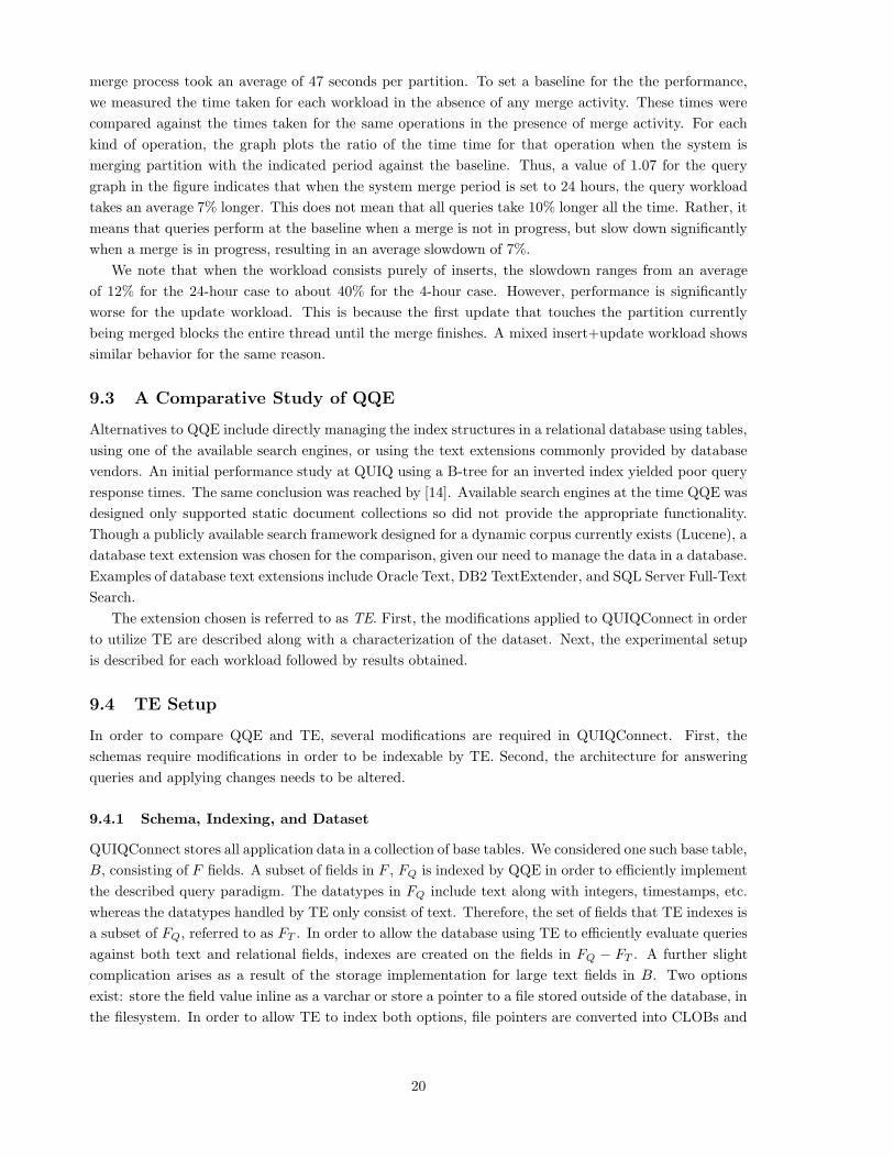
In order to compare QQE and TE, several modifications are required in QUIQConnect. First, the
schemas require modifications in order to be indexable by TE. Second, the architecture for answering
queries and applying changes needs to be altered.
9.4.1 Schema, Indexing, and Dataset
QUIQConnect stores all application data in a collection of base tables. We considered one such base table,
B, consisting of F fields. A subset of fields in F , FQ is indexed by QQE in order to efficiently implement
the described query paradigm. The datatypes in FQ include text along with integers, timestamps, etc.
whereas the datatypes handled by TE only consist of text. Therefore, the set of fields that TE indexes is
a subset of FQ, referred to as FT . In order to allow the database using TE to efficiently evaluate queries
against both text and relational fields, indexes are created on the fields in FQ − FT . A further slight
complication arises as a result of the storage implementation for large text fields in B. Two options
exist: store the field value inline as a varchar or store a pointer to a file stored outside of the database, in
the filesystem. In order to allow TE to index both options, file pointers are converted into CLOBs and
20
stored in extra fields that are added to B. A summary of the necessary modifications are summarized in
Figure 12. The schema, indexes, and file system usage is entirely consolidated into the database for TE.
Specifically, B contains 16,859 records and has a total of 16 fields in FT . Of those fields that are text
indexed, only 6 contain at least some data. Of the 6 fields that contain some data for indexing, only
2 fields contain a significant majority of the total data indexed. Since one field has consistently larger
values than the other, the fields are referred to as large and small fields.
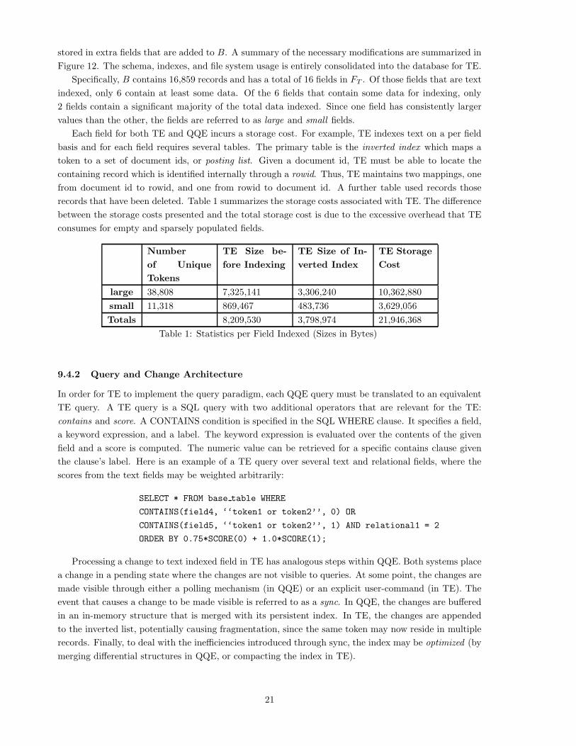
Each field for both TE and QQE incurs a storage cost. For example, TE indexes text on a per field
basis and for each field requires several tables. The primary table is the inverted index which maps a
token to a set of document ids, or posting list. Given a document id, TE must be able to locate the
containing record which is identified internally through a rowid. Thus, TE maintains two mappings, one
from document id to rowid, and one from rowid to document id. A further table used records those
records that have been deleted. Table 1 summarizes the storage costs associated with TE. The difference
between the storage costs presented and the total storage cost is due to the excessive overhead that TE
consumes for empty and sparsely populated fields.
Number
of Unique
Tokens
TE Size be-
fore Indexing
TE Size of In-
verted Index
TE Storage
Cost
large 38,808 7,325,141 3,306,240 10,362,880
small 11,318 869,467 483,736 3,629,056
Totals 8,209,530 3,798,974 21,946,368
Table 1: Statistics per Field Indexed (Sizes in Bytes)
9.4.2 Query and Change Architecture
In order for TE to implement the query paradigm, each QQE query must be translated to an equivalent
TE query. A TE query is a SQL query with two additional operators that are relevant for the TE:
contains and score. A CONTAINS condition is specified in the SQL WHERE clause. It specifies a field,
a keyword expression, and a label. The keyword expression is evaluated over the contents of the given
field and a score is computed. The numeric value can be retrieved for a specific contains clause given
the clause’s label. Here is an example of a TE query over several text and relational fields, where the
scores from the text fields may be weighted arbitrarily:
SELECT * FROM base table WHERE
CONTAINS(field4, ‘‘token1 or token2’’, 0) OR
CONTAINS(field5, ‘‘token1 or token2’’, 1) AND relational1 = 2
ORDER BY 0.75*SCORE(0) + 1.0*SCORE(1);
Processing a change to text indexed field in TE has analogous steps within QQE. Both systems place
a change in a pending state where the changes are not visible to queries. At some point, the changes are
made visible through either a polling mechanism (in QQE) or an explicit user-command (in TE). The
event that causes a change to be made visible is referred to as a sync. In QQE, the changes are buffered
in an in-memory structure that is merged with its persistent index. In TE, the changes are appended
to the inverted list, potentially causing fragmentation, since the same token may now reside in multiple
records. Finally, to deal with the inefficiencies introduced through sync, the index may be optimized (by
merging differential structures in QQE, or compacting the index in TE).
21
Workload TE QQE
1-Token-Low-Frequency-Header-Field 85 53
1-Token-Low-Frequency-Body-Field 92 57
1-Token-High-Frequency-Header-Field 314 72
1-Token-High-Frequency-Body-Field 614 79
2-Token-Low-Frequency-Header-Field 192 56
2-Token-Low-Frequency-Body-Field 195 59
2-Token-High-Frequency-Header-Field 672 76
2-Token-High-Frequency-Body-Field 1172 92
3-Token-Low-Frequency-Header-Field 302 66
3-Token-Low-Frequency-Body-Field 330 74
3-Token-High-Frequency-Header-Field 1225 101
3-Token-High-Frequency-Body-Field 2100 112
Figure 13: Comparing Query Performance
System Bulkload Insert Update Mixed Optimize
TE 142 4295 297 3425 82
QQE 179 59 83 67 107
Figure 14: Comparing Load and Update times (seconds)
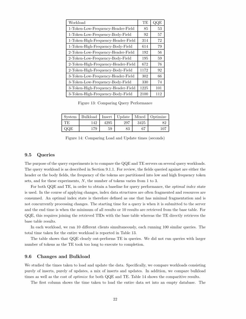
9.5 Queries
The purpose of the query experiments is to compare the QQE and TE servers on several query workloads.
The query workload is as described in Section 9.1.1. For review, the fields queried against are either the
header or the body fields, the frequency of the tokens are partitioned into low and high frequency token
sets, and for these experiments, N , the number of tokens varies from 1 to 3.
For both QQE and TE, in order to obtain a baseline for query performance, the optimal index state
is used. In the course of applying changes, index data structures are often fragmented and resources are
consumed. An optimal index state is therefore defined as one that has minimal fragmentation and is
not concurrently processing changes. The starting time for a query is when it is submitted to the server
and the end time is when the minimum of all results or 10 results are retrieved from the base table. For
QQE, this requires joining the retrieved TIDs with the base table whereas the TE directly retrieves the
base table results.
In each workload, we ran 10 different clients simultaneously, each running 100 similar queries. The
total time taken for the entire workload is reported in Table 13.
The table shows that QQE clearly out-performs TE in queries. We did not run queries with larger
number of tokens as the TE took too long to execute to completion.
9.6 Changes and Bulkload
We studied the times taken to load and update the data. Specifically, we compare workloads consisting
purely of inserts, purely of updates, a mix of inserts and updates. In addition, we compare bulkload
times as well as the cost of optimize for both QQE and TE. Table 14 shows the comparitive results.
The first column shows the time taken to load the entire data set into an empty database. The
22
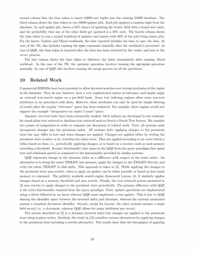
second column lists the time taken to insert 10000 new tuples into the existing 10MB database. The
third column shows the time taken to run 10000 update jobs. Each job updates a random tuple from the
database. In each update job, theres a 50% chance of updating the header field with a brand new value,
and the probability that any of the other fields get updated is a 20% each. The fourth column shows
the time taken to run a mixed workload of updates and inserts with 80% of the jobs being insert jobs.
For the Insert, Update and Mixed workloads, the time reported includes the time to sync the data. In
case of the TE, this includes running the sync command manually after the workload is processed. In
case of QQE, the time taken is reported after the data has been retrieved by the reader and sent to the
server process.
The last column shows the time taken to Optimize the index immediately after running Mixed
workload. In the case of the TE, the optimize operation involves running the optimize operation
manually. In case of QQE this involves running the merge process on all the partitions.
10 Related Work
Commercial RDBMSs have been extended to allow keyword searches over textual attributes of the tuples
in the database. They do not, however, have a very sophisticated notion of relevance, and simply apply
an external text-search engine on a per-field basis. Some text indexing engines allow some non-text
attributes to be associated with them. However, these attributes can only be used for simple filtering
of results after the regular “relevance” query has been evaluated. For example, these engines would not
support the example “inexpensive car under 5 years” query.
Dynamic inverted index have been extensively studied. Such indexes are developed in two contexts:
for stand-alone text retrieval or database text retrieval such as Oracle’s Oracle Text feature. We consider
two points of comparison in order to organize our discussion of related work. First, all systems must
incorporate changes into the persistent index. All systems defer applying changes to the persistent
store but may differ in how and when changes are applied. Changes are applied either by writing the
persistent store in-place or by rewriting the entire store. They are applied according to an event which is
either based on time, i.e., periodically applying changes, or is based on a resource such as used memory
exceeding a threshold. Second, functionality that arises in the QQE from the query paradigm that spans
text and relational queries is compared to the functionality provided by similar systems.
QQE represents change in the dynamic index as a difference with respect to the static index. An
alternative is to bring the entire TIDLIST into memory, apply the changes to the TIDLIST directly, and
write the entire TIDLIST to disk lazily. This approach is taken in [3]. While applying the changes to
the persistent store uses rewrite, when to apply an update can be either periodic or based on how much
memory is consumed. The publicly available search engine framework Lucene, [6, 5] similarly applies
changes based on a memory threshold and uses rewrite. Finally, the text retrieval system presented in
[4] uses rewrite to apply changes to the persistent store periodically. The primary difference with QQE
is the extra functionality required from the query paradigm. First, update operations are implemented
using a delete followed by an insert whereas QQE must implement a true update. This is due to QQE
sharing the identifier space between the inverted index and database, whereas the systems mentioned
assume a transient document identifier. Second, except for Lucene, the other systems assume a single
field record, i.e., a document, whereas QQE allows for many attributes per record.
The system described in [2] is a dynamic inverted index but changes are applied to the persistent
store using in-place writes. Similarly, the study in [13] considers various alternatives for applying changes
to the persistent store including a rewrite alternative. The results show that the throughput of applying
23
changes is higher using in-place writes at the cost of degrading query response time. Similarly, query
response time is lower when using rewrite since the inverted index is least fragmented whereas applying
changes degrades. In both systems, document or record identifiers are assumed to be transient so a true
update operation is not supported. In addition, multiple fields are not considered.
In terms of the query paradigm and maintanance issues arising from the integration with a relational
database, text extensions such as Oracle Text are appropriate for comparison with QQE. While QQE
maintains a single identifier space that spans the database and inverted index, Oracle Text maintains
disjoint identifier spaces that it translates between using two binary tables. Therefore, true updates are
supported in a manner comparable with QQE. Seperate identifier spaces offer flexibility and independence
for Oracle Text at the expense of requireing an identifier remapping during query processing. Another
difference is that changes to the persistent store are applied using in-place writes using a user invoked
function.
As an aside, similar techniques for deferring the application of change have arisen in database research.
The work in [11] argues for leaving a small area on disk for deferring changes so that the larger, existing
dataset can be better organized on disk. A technique for answering queries over the union of the
structures is also proposed. Data warehouses also need to accomodate changes to a structure that is
highly optimized for queries. The work in [8] proposes that the changes are similarly deferred and
merged into the main stcuture using a multi-level merge algorithm that depends on either hashing or
sorting. The Spider system [10, 9] uses an architecture similar to ours for supporting queries over
text data in a DBMS, but differs in its query paradigm and in many aspects of the implementation
approach. In particular, it applies updates in-place, as opposed to the defer and rewrite model that we
use. Also, the todo list is not accessed during query processing, resulting in a delay before data becomes
available for querying. [7] describes an implementation of the MOA object algebra which allows DBMS
and IR functionalities to be combined. This is implemented on top of the Monet [1] database system,
which implements a binary relation model. It is unclear how the performance characteristics of their
implemention would compare to the QQE.
11 Conclusion
In conclusion, QQE system is designed for applications that require the flexibility and intuitiveness of
text search combined with the structure present in a relational database. Furthermore, the system is
architected for environments that are dynamic but receive a significantly greater number of queries than
change requests. Furthermore, the anticipated applications requre query response time to be fasr.
The query paradigm that combines exact queries with approximate text queries is described. An
index into which text values are mapped to tokens and non-text values are mapped into pseudo-tokens
is described along with the processes and architecture required to efficiently query and maintain the
index. It is the combined management of these datatypes that allows QQE to efficiently implement the
combined query paradigm. Furthermore, the index allows concurrent querying and updates as a result
of a split index structure that defers the application of changes. The periodic, batched application of
changes is done by rewriting the index which greatly simplifies concurrency control and buys QQE the
benefits and flexibility of being self-organizing.
While multiple servers can be used to distribute query load, the requirement for full replication of the
index is wasteful. A parellization scheme that considers distributing chagnes is a significant candidate
for future work. Further work will also focus on the heuristics used for combining quality and match
and making the results more transparent to the user.
24
12 Acknowledgments
The authors would like to thank several people at QUIQ who contributed to the QUIQ system, and
to the implementation and testing of parts of QQE: Andrew Baptist, Matt Hanselman, Jim Kupsch,
Rajesh Raman, and Uri Shaft.
13 Bibliography
References
[1] P. Boncz and M. Kersten. Monet: an impressionist sketch of an advanced database system, proc.
biwitt, 1995.
[2] E.W. Brown, J.P. Callan, and W.B. Croft. Fast incremental indexing for full-text information
retrieval. In Proc. VLDB Conference, 1994.
[3] Tzi-Cker Chiueh and Lan Huang. Efficient real-time index updates in text retrieval systems (cite-
seer.nj.nec.com/chiueh99efficient.html).
[4] C. Clarke, G. Cormack, and F. Burkowski. Fast inverted indexes with on-line update (cite-
seer.nj.nec.com/clarke94fast.html), 1994.
[5] Doug Cutting. jakarta.apache.org/lucene.
[6] Doug Cutting and Jan Pedersen. Optimizations for dynamic inverted index maintenance. In Proc.
ACM SIGIR Conference, 1990.
[7] A. de Vries and A. Wilschut. The integration of ir and databases, proc. ifip working conference on
data semantics, 1999.
[8] H. V. Jagadish, I.S. Mumick, and A. Silberschatz. View maintenance issues for the chronicle data
model. In Proc. ACM PODS, 1995.
[9] D. Knaus and P. Schauble. The system architecture and the transaction concept of the spider ir
system. Data Engineering Bulletin, 19(1), 1996.
[10] P Schauble. Spider: A multiuser information retrieval system for semistructured and dynamic data.
In Proc. ACM SIGIR, 1993.
[11] D.G. Severance and G.M. Lohman. Differential files: Their application to the maintenance of large
databases. ACM TODS, 1(3):256–267, September 1976.
[12] A. Singhal, C. Buckley, and M. Mitra. Pivoted document length normalization. In Proc. ACM
SIGIR, 1996.
[13] Anthony Tomasic, Hector Garcıa-Molina, and Kurt Shoens. Incremental updates of inverted lists
for text document retrieval (citeseer.nj.nec.com/tomasic93incremental.html), 1994.
[14] Chun Zhang, Jeffrey F. Naughton, David J. DeWitt, Qiong Luo, and Guy M. Lohman. On sup-
porting containment queries in relational database management systems. In SIGMOD Conference,
2001.
25


![The NederDrone: a hybrid lift, hybrid energy hydrogen UAVhybrid energy [23]. 1.3. Hybrid Lift Hybrid Energy To combine the advantages of hybrid lift UAV with those of hybrid energy](https://img.pdfslide.net/doc/110x75/60d018b95ae9521d3952fc5b/the-nederdrone-a-hybrid-lift-hybrid-energy-hydrogen-uav-hybrid-energy-23-13.jpg)