Embed Size (px)
Citation preview
62
3The R environment
FIGURE 3.1All I want for Christmas is … some tasteful wallpaper
3.1. What will this chapter tell me? 1
At about 5 years old I moved from nursery (note that I moved, I was not ‘kicked out’ for showing my …) to primary school. Even though my older brother was already there, I remember being really scared about going. None of my nursery school friends were going to the same school and I was terrified about meeting lots of new children. I arrived in my classroom, and as I’d feared, it was full of scary children. In a fairly transparent ploy to
03-Field_R-4368-Ch-03.indd 62 11/02/2012 10:35:59 AM
Excerpt from: Field, A. P., Miles, J. N. V., & Field, Z. C. (2012). Discovering statistics using R: And sex and drugs and rock 'n' roll. London: Sage.
(c) Professor Andy P. Field, 2011

63CHAPTER 3 THE R ENV IRONMENT
make me think that I’d be spending the next 6 years building sand castles, the teacher told me to play in the sand pit. While I was nervously trying to discover whether I could build a pile of sand high enough to bury my head in, a boy came and joined me. He was Jonathan Land, and he was really nice. Within an hour he was my new best friend (5-year-olds are fickle …) and I loved school. Sometimes new environments seem scarier than they really are. This chapter introduces you to a scary new environment: R. The R environment is a generally more unpleasant environment in which to spend time than your normal environ-ment; nevertheless, we have to spend time there if we are to analyse our data. The purpose of this chapter is, therefore, to put you in a sand pit with a 5-year-old called Jonathan. I will orient you in your new home and reassure you that everything will be fine. We will explore how R works and the key windows in R (the console, editor and graphics/quartz windows). We will also look at how to create variables, data sets, and import and manipulate data.
3.2. Before you start 1
R is a free software environment for statistical computing and graphics. It is what’s known as ‘open source’, which means that unlike commercial software companies that protec-tively hide away the code on which their software is based, the people who developed R allow everyone to access their code. This open source philosophy allows anyone, anywhere to contribute to the software. Consequently, the capabilities of R dynamically expand as people from all over the world add to it. R very much embodies all that is good about the World Wide Web.
3.2.1. The R-chitecture 1
In essence, R exists as a base package with a reasonable amount of functionality. Once you have downloaded R and installed it on your own computer, you can start doing some data analysis and graphs. However, the beauty of R is that it can be expanded by download-ing packages that add specific functionality to the program. Anyone with a big enough brain and a bit of time and dedication can write a package for other people to use. These packages, as well as the software itself, are stored in a central location known as the CRAN (Comprehensive R Archive Network). Once a package is stored in the CRAN, anyone with an Internet connection can download it from the CRAN and install it to use within their own copy of R. R is basically a big global family of fluffy altruistic people contributing to the goal of producing a versatile data analysis tool that is free for everyone to use. It’s a statistical embodiment of The Beatles’ utopian vision of peace, love and humanity: a sort of ‘give ps a chance’.
The CRAN is central to using R: it is the place from where you download the software and any packages that you want to install. It would be a shame, therefore, if the CRAN were one day to explode or be eaten by cyber-lizards. The statistical world might col-lapse. Even assuming the cyber-lizards don’t rise up and overthrow the Internet, it is still a busy place. Therefore, rather than have a single CRAN location that everyone accesses, the CRAN is ‘mirrored’ at different places across the globe. ‘Mirrored’ simply means that there are identical versions of the CRAN scattered across the world. As a resident of the UK, I might access a CRAN location in the UK, whereas if you are in a different country you would likely access the copy of the CRAN in your own country (or one nearby). Bigger countries, such as the US, have multiple CRANs to serve them: the basic philosophy is to choose a CRAN that is geographically close to you.
03-Field_R-4368-Ch-03.indd 63 11/02/2012 10:35:59 AM
Excerpt from: Field, A. P., Miles, J. N. V., & Field, Z. C. (2012). Discovering statistics using R: And sex and drugs and rock 'n' roll. London: Sage.
(c) Professor Andy P. Field, 2011

64 D ISCOVER ING STAT IST ICS US ING R
Figure 3.2 shows schematically what we have just learnt. At the centre of the diagram is the CRAN: a repository of the base R software and hundreds of packages. People with big brains from all over the world write new packages and upload them into the CRAN for others to use. The CRAN itself is mirrored at different places across the globe (which just means there are multiple copies of it). As a user of R you download the software, and install any packages that you want to use via your nearest CRAN.
The idea of needing to install ‘packages’ into a piece of software to get it to do something for you might seem odd. However, whether you realize it or not many programs work in this way (just less obviously so). For example, the statistical package SPSS has a base ver-sion, but also has many modules (for example, the bootstrapping module, advanced sta-tistics, exact tests and so on). If you have not paid for these modules then certain options will be unavailable to you. Many students do not realize that SPSS has this modular format because they use it at a university and the university has paid for all of the modules that they need. Similarly, in Microsoft Excel you need to load the data analysis add-in before you can use certain facilities. R is not unusual in having a modular system, and in being modular it has enormous flexibility: as new statistical techniques are developed, contribu-tors can react quickly to produce a package for R; a commercial organization would likely take much longer to include this new technique.
3.2.2. Pros and cons of R 1
The main advantages of using R are that it is free, and it is a versatile and dynamic envi-ronment. Its open source format and the ability of statisticians to contribute packages to the CRAN mean that there are many things that you can do that cannot be done in com-mercially available packages. In addition, it is a rapidly expanding tool and can respond quickly to new developments in data analysis. These advantages make R an extremely powerful tool.
The downside to R is mainly ease of use. The ethos of R is to work with a command line rather than a graphical user interface (GUI). In layman’s terms this means typing instructions
FIGURE 3.2Users download R and install packages (uploaded by statisticians around the world) to their own computer via their nearest CRAN
03-Field_R-4368-Ch-03.indd 64 11/02/2012 10:36:01 AM
Excerpt from: Field, A. P., Miles, J. N. V., & Field, Z. C. (2012). Discovering statistics using R: And sex and drugs and rock 'n' roll. London: Sage.
(c) Professor Andy P. Field, 2011
65CHAPTER 3 THE R ENV IRONMENT
rather than pointing, clicking, and dragging things with a mouse. This might seem weird at first and a rather ‘retro’ way of working but I believe that once you have mastered a few fairly simple things, R’s written commands are a much more efficient way to work.
3.2.3. Downloading and installing R 1
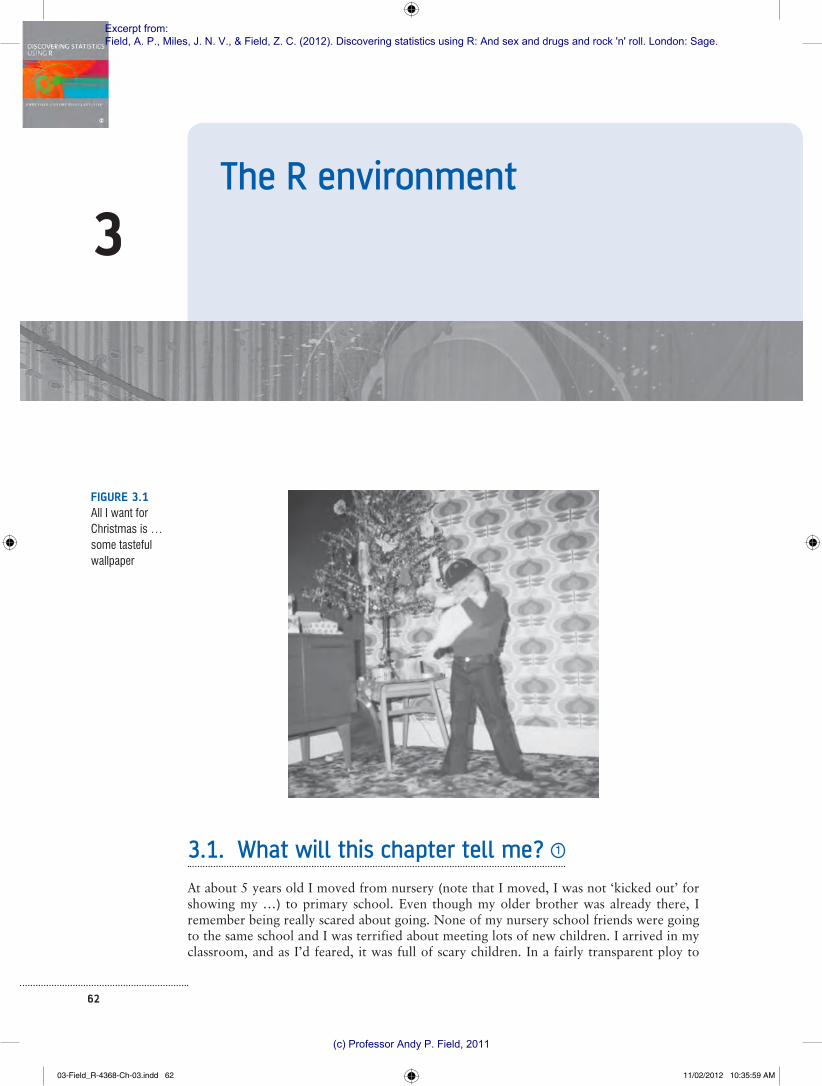
To install R onto your computer you need to visit the project website (http://www.R-project.org/). Figure 3.3 shows the process of obtaining the installation files. On the main project page, on the left-hand side, click on the link labelled ‘CRAN’. Remember from the previous section that there are various copies (mirrors) of the CRAN across the globe; therefore, the link to the CRAN will navigate you to a page of links to the various ‘mir-ror’ sites. Scroll down this list to find a mirror near to you (for example, in the diagram
FIGURE 3.3Downloading R
03-Field_R-4368-Ch-03.indd 65 11/02/2012 10:36:02 AM
Excerpt from: Field, A. P., Miles, J. N. V., & Field, Z. C. (2012). Discovering statistics using R: And sex and drugs and rock 'n' roll. London: Sage.
(c) Professor Andy P. Field, 2011
66 D ISCOVER ING STAT IST ICS US ING R
I have highlighted the mirror closest to me, http://www.stats.bris.ac.uk/R/) and click the link. Once you have been redirected to the CRAN mirror that you selected, you will see a web page that asks you which platform you use (Linux, MacOS or Windows). Click the link that applies to you. We’re assuming that most readers use either Windows or MacOS.
If you click on the ‘Windows’ link, then you’ll be taken to another page with some more links; click on ‘base’, which will redirect you to the webpage with the link to the setup file, once there click on the link that says ‘Download R 2.12.2 for Windows’,1 which will initi-ate the download of the R setup file. Once this file has been downloaded, double-click on it and you will enter a (hopefully) familiar install procedure.
If you click on the ‘MacOS’ link you will be taken directly to a page from where you can download the install package by clicking on the link labelled ‘R-2.12.2.pkg’ (please read the footnote about version numbers). Clicking this link will download the install file; once downloaded, double-click on it and you will enter the normal MacOS install procedure.
3.2.4. Versions of R 1
At the time of writing, the current version of R is 2.12.2; however, the software updates fairly regularly so we are confident that by the time anyone is actually read-
ing this, there will be a newer release (possibly several). Notice that the format of the version number is major.minor.patch, which means that we are currently on major version 2, minor version 12 and patch 2. Changes in the patch number happen fairly frequently and usually reflect fixes of minor bugs (so, for example, version 2.12.3 will come along pretty quickly but won’t really be a substantial change to the software, just some housekeeping). Minor versions come less regu-larly (about every 6 months) and still reflect a collection of bug fixes and minor housekeeping that keeps the software running optimally. Major releases are quite rare (the switch from version 1 to version 2 happened in 2006). As such, apart from minor fixes, don’t worry if you are using a more recent version of R than the one we’re using: it won’t make any difference, or shouldn’t do. The best advice is to update every so often but other than that don’t worry too much about which version you’re using; there are more important things in life to worry about.
3.3. Getting started 1
Once you have installed R you can activate it in the usual way. In windows go to the start menu (the big windows icon in the bottom left of the screen) select ‘All Programs’, then scroll down to the folder labelled ‘R’, click on it, and then click on the R icon (Figure 3.4). In MacOS, go to your ‘Applications’ folder, scroll down to the R icon and click on it (Figure 3.4).
1 At the time of writing the current version of R is 2.12.2, but by the time you read this book there will have been an update (or possibly several), so don’t be surprised if the ‘2.12.2’ in the link has changed to a different number. This difference is not cause for panic, the link will simply reflect the version number of R.
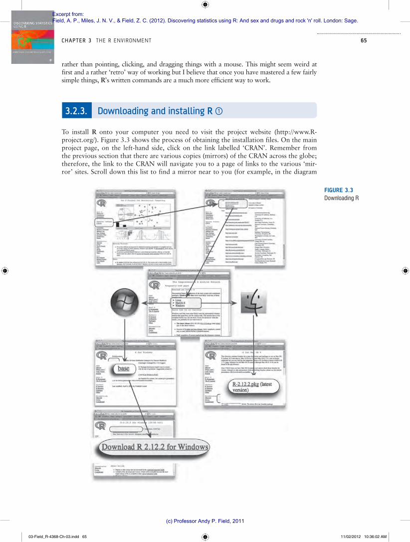
Which version ofR do I needed touse this book?
Which version ofR do I needed touse this book?
03-Field_R-4368-Ch-03.indd 66 11/02/2012 10:36:03 AM
Excerpt from: Field, A. P., Miles, J. N. V., & Field, Z. C. (2012). Discovering statistics using R: And sex and drugs and rock 'n' roll. London: Sage.
(c) Professor Andy P. Field, 2011

67CHAPTER 3 THE R ENV IRONMENT
3.3.1. The main windows in R 1
There are three windows that you will use in R. The main window is called the console (Figure 3.4) and it is where you can both type commands and see the results of executing these commands (in other words, see the output of your analysis). Rather than writing commands directly into the console you can also write them in a separate window (known as the editor window). Working with this window has the advantage that you can save col-lections of commands as a file that you can reuse at another point in time (perhaps to rerun the analysis, or to run a similar analysis on a different set of data). I generally tend to work in this way rather than typing commands into the console because it makes sense to me to save my work in case I need to replicate it, and as you do more analyses you begin to have a repository of R commands that you can quickly adapt when running a new analysis. Ultimately you have to do what works for you. Finally, if you produce any graphics or graphs they will appear in the graphics window (this window is labelled quartz in MacOS).
FIGURE 3.4Getting R started
3.3.2. Menus in R 1
Once R is up and running you’ll notice a menu bar similar to the ones you might have seen in other programs. Figure 3.4 shows the console window and the menu bar associated with this window. There are some subtle differences between Windows and MacOS versions of R and we will look at each version in the following two sections. At this stage, simply note that there are several menus at the top of the screen (e.g., ) that can be activated
03-Field_R-4368-Ch-03.indd 67 11/02/2012 10:36:04 AM
Excerpt from: Field, A. P., Miles, J. N. V., & Field, Z. C. (2012). Discovering statistics using R: And sex and drugs and rock 'n' roll. London: Sage.
(c) Professor Andy P. Field, 2011

71CHAPTER 3 THE R ENV IRONMENT
Table 3.3 Overview of the menus in R for MacOS
MenuFile: This menu allows you to do general things such as saving scripts or graphs. Likewise, you can open previously saved files and print graphs, data or output. In essence, it contains all of the options that are customarily found in File menus.
Edit: This menu contains edit functions such as cut and paste. From here you can also clear the console (i.e., remove all of the text from it), execute commands, find a particular bit of text and so on.
Format: This menu lets you change the text styles used (colour, font, etc.).
Workspace: This menu enables you to save the workspace (i.e., analysis output – see section 3.4), load an old workspace or browse your recent workspace files.
Packages & Data: This menu is very important because it is where you load, install and update packages.
Misc: This menu enables you to set or change the working directory. The working directory is the default location where R will search for and save files (see section 3.4.4).
Window: If you have multiple windows, this menu allows you to change how the windows in R are arranged.
Help: This is an invaluable menu because it offers you a searchable repository of help and frequently asked questions.
3.4. Using R 1
3.4.1. Commands, objects and functions 1
I have already said that R uses ‘commands’ that are typed into the console window. As such, unlike other data analysis packages with which you might be familiar (e.g., SPSS, SAS), there are no friendly dialog boxes that you can activate to run analyses. Instead, everything you want to do has to be typed into the console (or executed from a script file). This might sound like about as much fun as having one of the living dead slowly chewing on your brain, but there are advantages to working in this way: although there is a steep initial learning curve, after time it becomes very quick to run analyses.
Commands in R are generally made up of two parts: objects and functions. These are separated by ‘<-’, which you can think of as meaning ‘is created from’. As such, the general form of a command is:
Object<-function
Which means ‘object is created from function’. An object is anything created in R. It could be a variable, a collection of variables, a statistical model, etc. Objects can be single values (such as the mean of a set of scores) or collections of information; for example, when you run an analysis, you create an object that contains the output of that analysis, which means that this object contains many different values and variables. Functions are the things that you do in R to create your objects. In the console, to execute a command you simply type it into the console and press the return key. (You can put more than one command on a single line if you prefer – see R’s Souls’ Tip 3.2)
03-Field_R-4368-Ch-03.indd 71 11/02/2012 10:36:05 AM
Excerpt from: Field, A. P., Miles, J. N. V., & Field, Z. C. (2012). Discovering statistics using R: And sex and drugs and rock 'n' roll. London: Sage.
(c) Professor Andy P. Field, 2011

72 D ISCOVER ING STAT IST ICS US ING R
Table 3.4 Overview of the icons in R for MacOS
Icon Description Console EditorClicking this button stops the R processor from whatever it is doing. !
Clicking this button opens a dialog box that enables you to select a previously saved script or data file. !
Clicking this button opens a new graphics (quartz) window.!
Clicking this button opens the X11 window; X11 is a device that some R packages use. !
Clicking this button opens a dialog box into which you can enter your system password. This will enable R to run system commands. Frankly, I have never touched this button and I suspect it is to be used only by people who actually know what they’re doing.
!
Clicking this button activates a sidebar on the console window that lists all of your recently executed commands. !
Clicking this button opens the Preferences dialog box, from which you can change the console colours (amongst other things).
!
Clicking this button opens a dialog box from which you can select and open a previously saved script file. This file will open in the editor window.
!
Clicking this button opens a new editor window in which you can create a new script file. !
This icon activates a dialog box for printing whatever you are currently working on (what is printed depends on which window is active).
! !
Clicking this button saves the script file that you’re working on. If you have not already saved the file, clicking this button activates a Save As … dialog box.
!
Clicking this button quits R.!
Figure 3.5 shows a very simple example in which we have created an object called ‘metal-lica’, which is made up of the four band members’ (pre 2001) names. The function used is the concatenate function or c(), which groups things together. As such, we have written each band member’s name (in speech marks and separated by commas), and by enclosing them in c() we bind them into a single entity or object, which we have called ‘metallica’. If we type this command into the console then when we hit the return key on the keyboard the object that we have called ‘metallica’ is created. This object is stored in memory so we can refer back to it in future commands. Throughout this book, we denote commands entered into the command line in this way:
03-Field_R-4368-Ch-03.indd 72 11/02/2012 10:36:05 AM
Excerpt from: Field, A. P., Miles, J. N. V., & Field, Z. C. (2012). Discovering statistics using R: And sex and drugs and rock 'n' roll. London: Sage.
(c) Professor Andy P. Field, 2011

73CHAPTER 3 THE R ENV IRONMENT
FIGURE 3.5Using the command line in R
R ’s Souls ’ T ip 3 .2 Running multiple commands at once 1
The command line format of R tends to make you think that you have to run commands one at a time. Even if you use the R editor it is tempting to put different commands on a new line. There’s nothing wrong with doing this, and it can make it easier to decipher your commands if you go back to a long script months after you wrote it. However, it can be useful to run several commands in a single line. Separating them with a semicolon does this. For example, the two commands:
metallica<-metallica[metallica != "Jason"]
metallica<-c(metallica, "Rob")
can be run in a single line by using a semicolon to separate them:
metallica<-metallica[metallica != "Jason"]; metallica<-c(metallica, "Rob")
03-Field_R-4368-Ch-03.indd 73 11/02/2012 10:36:06 AM
Excerpt from: Field, A. P., Miles, J. N. V., & Field, Z. C. (2012). Discovering statistics using R: And sex and drugs and rock 'n' roll. London: Sage.
(c) Professor Andy P. Field, 2011
74 D ISCOVER ING STAT IST ICS US ING R
metallica<-c("Lars","James","Jason","Kirk")
which follows the style of the MacOS version of the R editor (the Windows version of the R editor uses plain text so don’t be concerned about the fact that you won’t see coloured text in Windows).
Now we have created an object called ‘metallica’ we can do things with it. First, we can have a look at its contents by typing ‘metallica’ (or ‘print(metallica)’ works too) into the command line and hitting the return key:
metallica
The contents of the object ‘metallica’ will be displayed in the console window. Throughout the book we display output as follows:
[1] "Lars" "James" "Jason" "Kirk"
Note that R has printed into the console the contents of the object ‘metallica’, and the contents are simply the four band members’ names. You need to be very careful when you type commands and create objects in R, because it is case sensitive (see R’s Souls’ Tip 3.3).
R ’s Souls ’ T ip 3 .3 R is case sensitive 1
R is case sensitive, which means that if the same things are written in upper or lower case, R thinks that they are completely different things. For example, we created a variable called metallica; if we asked to see the con-tents of Metallica (note the capital M), R would tell us that this object didn’t exist. If we wanted to completely confuse ourselves we could actually create a variable called Metallica (with a capital M) and put different data into it than in the variable metallica (with a small m), and R would have no problem with us doing so. As far as R is concerned, metallica and Metallica are as different to each other as variables called earwax and doseOfBellendium.
This case sensitivity can create problems if you don’t pay attention. Functions are generally lower case so you just need to avoid accidentally using capitals, but every so often you find a function that has a capital letter (such as as.Date() used in this chapter) and you need to make sure you have typed it correctly. For example, if you want to use the function data.frame() but type data.Frame() or Data.Frame() you will get an error. If you get an error, check that you have typed any functions or variable names exactly as they should be.
We can do other things with our newly created object too. The Metallica fans amongst you will probably be furious at me for listing the pre 2001 line up of the band. In 2001 bassist Jason Newstead left the band and was replaced by Rob Trujillo. Even as I type, there are hoards of Metallica fans with precognition about the contents of this book queuing outside my house and they have dubbed me unforgiven. Personally I’m a big fan of Rob Trujillo, he’s given the band a solid kick up the backside, and so let’s put him in his rightful place in the band. We currently have a ‘metallica’ object that contains Jason. First we can change our object to eject Jason (harsh, I know). To get rid of Jason in R we can use this command:
metallica<-metallica[metallica != "Jason"]
This just means that we’re re-creating the object ‘metallica’, the ‘<-‘ means that ‘we’re creating it from’ and our function is metallica[metallica != “Jason”] which means ‘use the object metallica, but get rid of (!=) Jason’. A simple line of text and Jason is gone, which
03-Field_R-4368-Ch-03.indd 74 11/02/2012 10:36:06 AM
Excerpt from: Field, A. P., Miles, J. N. V., & Field, Z. C. (2012). Discovering statistics using R: And sex and drugs and rock 'n' roll. London: Sage.
(c) Professor Andy P. Field, 2011
75CHAPTER 3 THE R ENV IRONMENT
was probably a lot less hassle than his actual ousting from the band. If only Lars and James had come to me for advice. If we have a look at our ‘metallica’ object now we’ll see that it contains only three names. We can do this by simply typing ‘metallica’ and hitting the return key. Below shows the command and the output:
metallica
[1] "Lars" "James" "Kirk"
Now let’s add Rob Trujillo to the band. To do this we can again create an object called ‘metallica’ (which will overwrite our previous object), and we can use the concatenate com-mand to take the old ‘metallica’ object and add “Rob” to it. The command looks like this:
metallica<-c(metallica, "Rob")
If we execute this command (by pressing return) and again look at the contents of ‘metal-lica’ we will see that Rob has been added to the band:
metallica
[1] "Lars" "James" "Kirk" "Rob"
SELF-TEST
9 Create an object that represents your favourite band (unless it’s Metallica, in which case use your second favourite band) and that contains the names of each band member. If you don’t have a favourite band, then create an object called friends that contains the names of your five best friends.
3.4.2. Using scripts 1
Although you can execute commands from the console, I think it is better to write com-mands in the R editor and execute them from there. A document of commands written in the R editor is known as a script. There are several advantages to this way of working. First, at the end of your session you can save the script file, which can be reloaded in the future if you need to re-create your analysis. Rerunning analyses, therefore, becomes a matter of loading a file and hitting a few buttons – it will take less than 10 seconds. Often in life you need to run analyses that are quite similar to ones that you have run before; if you have a repository of scripts then it becomes fairly quick to create new ones by editing an existing one or cutting and pasting commands from existing scripts and then editing the variable names. Personally I find that using old scripts to create new ones speeds things up a lot, but this could be because I’m pretty hopeless at remembering how to do things in R. Finally, I often mess things up and run commands that throw error messages back in my face; if these commands are written directly into the console then you have to rewrite the whole command (or cut and paste the wrong command and edit it), whereas if you ran the com-mand from the editor window then you can edit the command directly without having to cut and paste it (or rewrite it), and execute it. Again, it’s a small saving in time, but these savings add up until eventually the savings outweigh the actual time you’re spending doing the task and then time starts to run backwards. I was 56 when I started writing this book, but thanks to using the editor window in R I am now 37.
03-Field_R-4368-Ch-03.indd 75 11/02/2012 10:36:06 AM
Excerpt from: Field, A. P., Miles, J. N. V., & Field, Z. C. (2012). Discovering statistics using R: And sex and drugs and rock 'n' roll. London: Sage.
(c) Professor Andy P. Field, 2011

76 D ISCOVER ING STAT IST ICS US ING R
Figure 3.6 shows how to execute commands from the editor window. Assuming you have written some commands, all you need to do is to place the cursor in the line contain-ing the command that you want to execute, or if you want to execute many commands in one go then highlight a block of commands by dragging over them while holding down the left mouse button. Once your commands are highlighted, you can execute them in one of several ways.
In Windows, you have a plethora of choices: you can (1) click on ; (2) click the right mouse button while in the editor window to activate a menu, then click with the left mouse button on the top option which is to run the command (see Figure 3.6); (3) go through the main menus by selecting Edit!Run line or selection; or (4) press and hold down theCtrl key, and while holding it down press and release the letter R on the keyboard (this is by far the quickest option). In the book we notate pressing a key while another is held down as ‘hold + press’, for example Ctrl + R means press the R key while holding down the Ctrl key.
In MacOS you can run the highlighted commands, or the current line, through the menus by selecting Edit!Execute, but as with Windows the keyboard shortcut is much quicker: press and hold down the cmd key (a), and while holding it down press and release the return key ("). In case you skipped the previous paragraph, we will notate pressing a key while another is held down as ‘hold + press’, for example a + " means press the " key while holding down the a.
You’ll notice that the commands appear in the console window as they are executed, along with any consequences of those commands (for example, if one of your commands asks to view an object the contents will be printed in the console just the same as if you had typed the command directly into the console).
3.4.3. The R workspace 1
As you work on a given data set or analysis, you will create many objects, all of which are stored in memory. The collection of objects and things you have created in a session is known as your workspace. When you quit R it will ask you if you want to save your current workspace. If you choose to save the workspace then you are saving the contents of the
FIGURE 3.6Executing commands from the R editor window
03-Field_R-4368-Ch-03.indd 76 11/02/2012 10:36:07 AM
Excerpt from: Field, A. P., Miles, J. N. V., & Field, Z. C. (2012). Discovering statistics using R: And sex and drugs and rock 'n' roll. London: Sage.
(c) Professor Andy P. Field, 2011

77CHAPTER 3 THE R ENV IRONMENT
console window and any objects that have been created. The file is known as an R image and is saved in a file with .RData at the end. You can save the workspace at any time using the File!Save Workspace … menu in Windows or in MacOS make sure you are in the console window and select File!Save As ….
3.4.4. Setting a working directory 2
By default, when you try to do anything (e.g., open a file) from R it will go to the directory in which the program is stored on your computer. This is fine if you happen to store all of your data and output in that folder, but it is highly unlikely that you do. If you don’t then every time you want to load or save a file you will find yourself wasting time using the menus to navigate around your computer to try to find files, and you will probably lose track of things you save because they have been dumped in R’s home folder. You will also end up having to specify the exact file path for every file you save/access. For example, assuming that you’re using Windows, your user name is ‘Andy F’ (because you’ve stolen my identity), you have a folder in your main documents folder called ‘Data’ and within that you have another folder called ‘R Book Examples’, then if you want to access this folder (to save or load a file) you’d have to use this file path:
C:/Users/Andy F/Documents/Data/R Book Examples
So, to load a file called data.dat from this location you would need to execute the follow-ing command:
myData = read.delim("C:/Users/Andy F/Documents/Data/R Book Examples/data.dat")
Don’t worry about what this command means (we’ll get to that in due course), I just want you to notice that it is going to get pretty tedious to keep typing ‘C:/Users/Andy F/Documents/Data/R Book Examples’ every time you want to load or save something.
If you use R as much as I do then all this time typing locations has two consequences: (1) all those seconds have added up and I have probably spent weeks typing file paths when I could have been doing something useful like playing my drum kit; (2) I have increased my chances of getting RSI in my wrists, and if I’m going to get RSI in my wrists I can think of more enjoyable ways to achieve it than typing file paths (drumming again, obviously).
The best piece of advice I can give you is to establish a working directory at the beginning of your R session. This is a directory in which you want to store your data files, any scripts associated with the analysis or your workspace. Basically, anything to do with a session. To begin with, create this folder (in the usual way in Windows or MacOS) and place the data files you’ll be using in that folder. Then, when you start your session in R change the working directory to be the folder that you have just created. Let’s assume again that you’re me (Andy F), that you have a folder in ‘My Documents’ called ‘Data’ and within that you have created a folder called ‘R Book Examples’ in which you have placed some data files that you want to analyse. To set the working directory to be this folder, we use the setwd() command to specify this newly created folder as the working directory:
setwd("C:/Users/Andy F/Documents/Data/R Book Examples")
By executing this command, we can now access files in that folder directly without having to reference the full file path. For example, if we wanted to load our data.dat file again, we can now execute this command:
myData = read.delim("data.dat")
03-Field_R-4368-Ch-03.indd 77 11/02/2012 10:36:07 AM
Excerpt from: Field, A. P., Miles, J. N. V., & Field, Z. C. (2012). Discovering statistics using R: And sex and drugs and rock 'n' roll. London: Sage.
(c) Professor Andy P. Field, 2011
78 D ISCOVER ING STAT IST ICS US ING R
Compare this command with the one we wrote earlier; it is much shorter because we can now specify only the file name safe in the knowledge that R will automatically try to find the file in ‘C:/Users/Andy F/Documents/Data/R Book Examples’. If you want to check what the working directory is then execute this command:
getwd()
Executing this command will display the current working directory in the console window.2
In MacOS you can do much the same thing except that you won’t have a C drive. Assuming you are likely to work in your main user directory, the easiest thing to do is to use the ‘ ~ ’ symbol, which is a shorthand for your user directory. So, if we use the same file path as we did for Windows, we can specify this as:
setwd("~/Documents/Data/R Book Examples")
The ~ specifies the MacOS equivalent of ‘C:/Users/Andy F’. Alternatively, you can navigate to the directory that you want to use using the Misc!Change Working Directory menu path (or a + D).
Throughout the book I am going to assume that for each chapter you have stored the data files somewhere that makes sense to you and that you have set this folder to be your working directory. If you do not do this then you’ll find that commands that load and save files will not work.
3.4.5. Installing packages 1
Earlier on I mentioned that R comes with some base functions ready for you to use. However, to get the most out of it we need to install packages that enable us to do particu-lar things. For example, in the next chapter we look at graphs, and to create the graphs in that chapter we use a package called ggplot2. This package does not come pre-installed in R so to work through the next chapter we would have to install ggplot2 so that R can access its functions.
You can install packages in two ways: through the menus or using a command. If you know the package that you want to install then the simplest way is to execute this command:
install.packages("package.name")
in which ‘package.name’ is replaced by the name of the package that you’d like installed. For example, we have (hopefully) written a package containing some functions that are used in the book. This package is called DSUR, therefore, to install it we would execute:
install.packages("DSUR")
Note that the name of the package must be enclosed in speech marks.Once a package is installed you need to reference it for R to know that you’re using it.
You need to install the package only once3 but you need to reference it each time you start a new session of R. To reference a package, we simply execute this general command:
library(package.name)
2 In Windows, the filepaths can also be specified using ‘\\’ to indicate directories, so that “C:/Users/Andy F/Docu-ments/Data/R Book Examples” is exactly the same as “C: \\Users\\Andy F\\Documents\\Data\\R Book Examples”. R tends to return filepaths in the ‘\\’ form, but will accept it if you specify them using ‘/’. Try not to be confused by these two different formats. MacOS users don’t have these tribulations.
3 This isn’t strictly true: if you upgrade to a new version of R you will have to reinstall all of your packages again.
03-Field_R-4368-Ch-03.indd 78 11/02/2012 10:36:07 AM
Excerpt from: Field, A. P., Miles, J. N. V., & Field, Z. C. (2012). Discovering statistics using R: And sex and drugs and rock 'n' roll. London: Sage.
(c) Professor Andy P. Field, 2011
79CHAPTER 3 THE R ENV IRONMENT
in which ‘package.name’ is replaced by the name of the package that you’d like to use. Again, if we want to use the DSUR package we would execute:
library(DSUR)
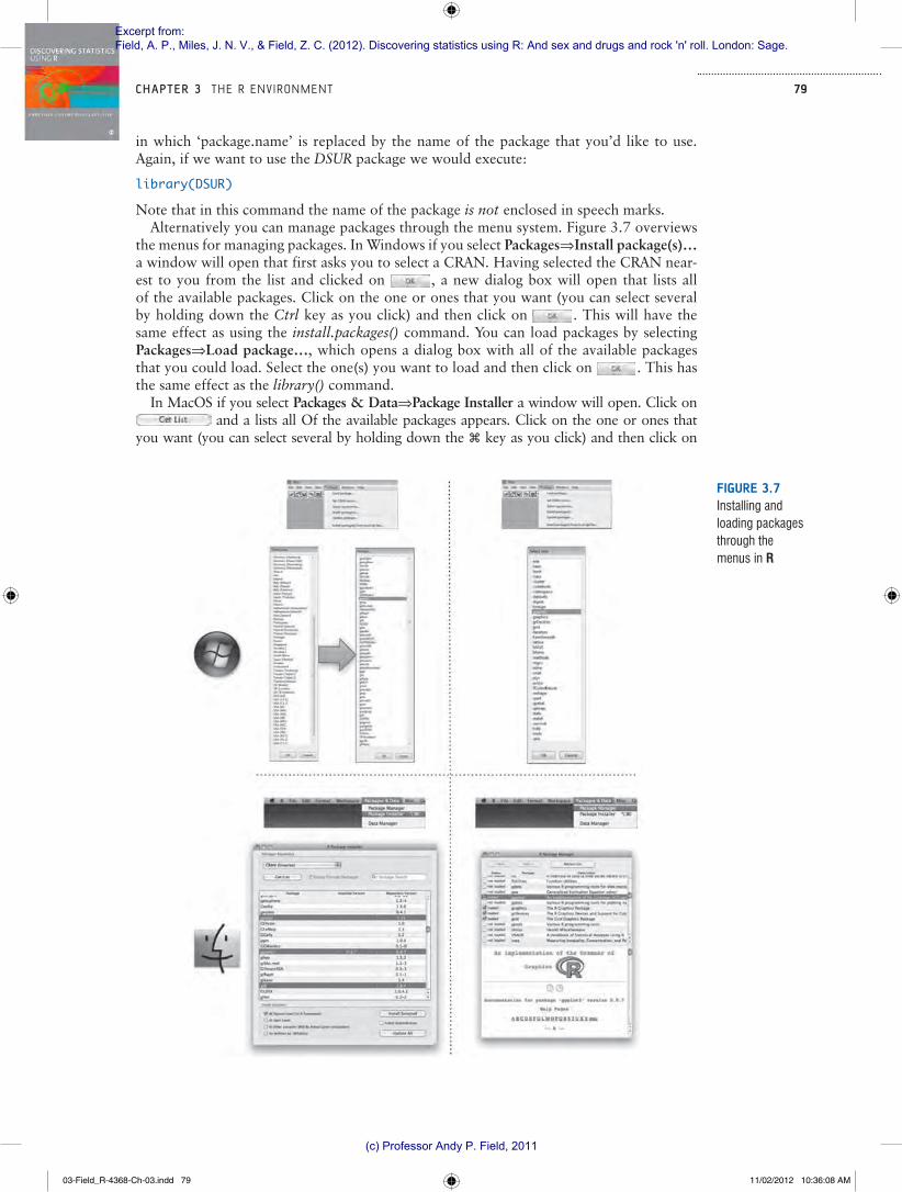
Note that in this command the name of the package is not enclosed in speech marks.Alternatively you can manage packages through the menu system. Figure 3.7 overviews
the menus for managing packages. In Windows if you select Packages!Install package(s)… a window will open that first asks you to select a CRAN. Having selected the CRAN near-est to you from the list and clicked on , a new dialog box will open that lists all of the available packages. Click on the one or ones that you want (you can select several by holding down the Ctrl key as you click) and then click on . This will have the same effect as using the install.packages() command. You can load packages by selecting Packages!Load package…, which opens a dialog box with all of the available packages that you could load. Select the one(s) you want to load and then click on . This has the same effect as the library() command.
In MacOS if you select Packages & Data!Package Installer a window will open. Click on and a lists all Of the available packages appears. Click on the one or ones that
you want (you can select several by holding down the a key as you click) and then click on
FIGURE 3.7Installing and loading packages through the menus in R
03-Field_R-4368-Ch-03.indd 79 11/02/2012 10:36:08 AM
Excerpt from: Field, A. P., Miles, J. N. V., & Field, Z. C. (2012). Discovering statistics using R: And sex and drugs and rock 'n' roll. London: Sage.
(c) Professor Andy P. Field, 2011
80 D ISCOVER ING STAT IST ICS US ING R
R ’s Souls ’ T ip 3 .4 Disambiguating functions 1
Occasionally you might stumble across two functions in two different packages that have the same name. For example, there is a recode() function in both the Hmisc and car packages. If you have both packages loaded and you try to use recode(), R won’t know which one to use or will have a guess (perhaps incorrectly). This situation is easy to rectify: you can specify the package when you use the function as follows:
package::function()
For example, if we want to use the recode() function in the car package we would write:
car::recode()
but to use the one in Hmisc we would write:
Hmisc::recode()
Here is an example where we recode a variable using recode() from the car package:
variableName <-car::recode(variableName, "2=0;0=2")
. This will have the same effect as using the install.packages() command. You can load packages by selecting Packages & Data!Package Manager, which opens a dialog box with all of the available packages that you could load. Click on the tick boxes next to the one(s) you want to load. This has the same effect as the library() command.
One entertaining (by which I mean annoying) consequence of any Tom, Dick or Harriet being able to contribute packages to R is that you sometimes encounter useful functions that have the same name as different functions in different packages. For example, there is a recode() function that exists in both the Hmisc and car packages. Therefore, if you have both of these packages loaded you will need to tell R which particular recode function you want to use (see R’s Souls’ Tip 3.4).
3.4.6. Getting help 1
There is an enormous amount of information on the Internet about using R, and I gener-ally find that if I get stuck I can find help with a quick Google (or whatever search engine you use) search. However, there is help built into R as well. If you are using a particular function and you want to know more about it then you can get help by executing the help() command:
help(function)
or by executing:
?function
In both cases function is the name of the function about which you need help. For example, we used the concatenate function earlier on, c(), if we wanted help with this function we could execute either:
help(c)
or
?c
03-Field_R-4368-Ch-03.indd 80 11/02/2012 10:36:08 AM
Excerpt from: Field, A. P., Miles, J. N. V., & Field, Z. C. (2012). Discovering statistics using R: And sex and drugs and rock 'n' roll. London: Sage.
(c) Professor Andy P. Field, 2011

81CHAPTER 3 THE R ENV IRONMENT
These commands open a new window with the help documentation for that function. Be aware that the help files are active only if you have loaded the package to which the func-tion belongs. Therefore, if you try to use help but the help files are not found, check that you have loaded the relevant package with the library() command.
3.5. Getting data into R 1
3.5.1. Creating variables 1
You can enter data directly into R. As we saw earlier on, you can use the c() function to cre-ate objects that contain data. The example we used was a collection of names, but you can do much the same with numbers. Earlier we created an object containing the names of the four members of metallica. Let’s do this again, but this time call the object metallicaNames. We can create this object by executing the following command:
metallicaNames<-c("Lars","James","Kirk","Rob")
We now have an object called metallicaNames containing the band members’ names. When we create objects it is important to name them in a meaningful way and you should put some thought into the names that you choose (see R’s Souls’ Tip 3.7).
Let’s say we wanted another object containing the ages of each band member. At the time of writing, their ages are 47, 47, 48 and 46, respectively. We can create a new object called metallicaAges in the same way as before, by executing:
metallicaAges<-c(47, 47, 48, 46)
Notice that when we specified names we placed the names in quotes, but when we entered their ages we did not. The quotes tell R that the data are not numeric. Variables that consist of data that are text are known as string variables. Variables that contain data that are numbers are known as numeric variables. R and its associated packages tend to be able to treat data fairly intelligently. In other words, we don’t need to tell R that a variable is numeric or not, it sort of works it out for itself – most of the time at least. However, string values should always be placed in quotes, and numeric val-ues are never placed in quotes (unless you want them to be treated as text rather than numbers).
3.5.2. Creating dataframes 1
We currently have two separate objects: metallicaNames and metallicaAges. Wouldn’t it be nice to combine them into a single object? We can do this by creating a dataframe. You can think of a dataframe as a spreadsheet (so, like the contents of the data editor in SPSS, or a worksheet in Excel). It is an object containing variables. There are other ways to combine variables in R but dataframes are the way we will most commonly use because of their ver-satility (R’s Souls’ Tip 3.5). If we want to combine metallicaNames and metallicaAges into a dataframe we can use the data.frame() function:
metallica<-data.frame(Name = metallicaNames, Age = metallicaAges)
In this command we create a new object (called metallica) and we create it from the func-tion data.frame(). The text within the data.frame() command tells R how to build the dataframe. First it tells R to create an object called ‘Name’, which is equal to the existing
03-Field_R-4368-Ch-03.indd 81 11/02/2012 10:36:08 AM
Excerpt from: Field, A. P., Miles, J. N. V., & Field, Z. C. (2012). Discovering statistics using R: And sex and drugs and rock 'n' roll. London: Sage.
(c) Professor Andy P. Field, 2011
82 D ISCOVER ING STAT IST ICS US ING R
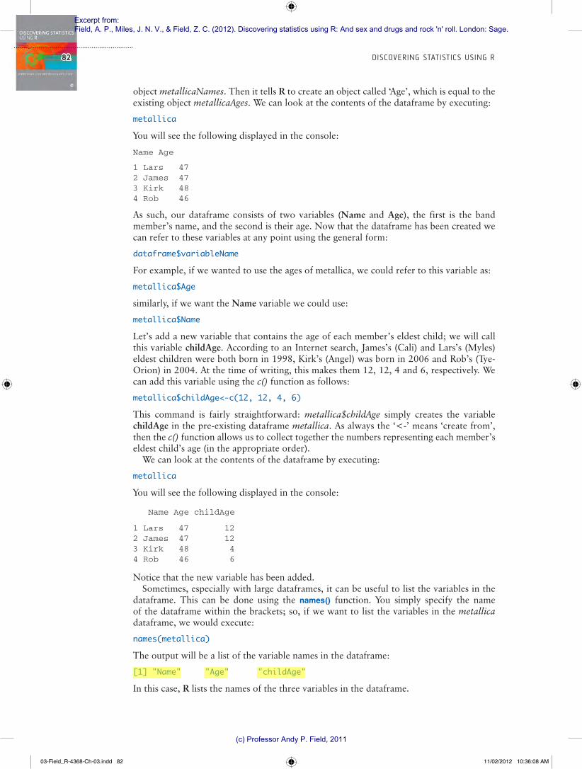
object metallicaNames. Then it tells R to create an object called ‘Age’, which is equal to the existing object metallicaAges. We can look at the contents of the dataframe by executing:
metallica
You will see the following displayed in the console:
Name Age
1 Lars 472 James 473 Kirk 484 Rob 46
As such, our dataframe consists of two variables (Name and Age), the first is the band member’s name, and the second is their age. Now that the dataframe has been created we can refer to these variables at any point using the general form:
dataframe$variableName
For example, if we wanted to use the ages of metallica, we could refer to this variable as:
metallica$Age
similarly, if we want the Name variable we could use:
metallica$Name
Let’s add a new variable that contains the age of each member’s eldest child; we will call this variable childAge. According to an Internet search, James’s (Cali) and Lars’s (Myles) eldest children were both born in 1998, Kirk’s (Angel) was born in 2006 and Rob’s (Tye-Orion) in 2004. At the time of writing, this makes them 12, 12, 4 and 6, respectively. We can add this variable using the c() function as follows:
metallica$childAge<-c(12, 12, 4, 6)
This command is fairly straightforward: metallica$childAge simply creates the variable childAge in the pre-existing dataframe metallica. As always the ‘<-’ means ‘create from’, then the c() function allows us to collect together the numbers representing each member’s eldest child’s age (in the appropriate order).
We can look at the contents of the dataframe by executing:
metallica
You will see the following displayed in the console:
Name Age childAge
1 Lars 47 122 James 47 123 Kirk 48 44 Rob 46 6
Notice that the new variable has been added.Sometimes, especially with large dataframes, it can be useful to list the variables in the
dataframe. This can be done using the names() function. You simply specify the name of the dataframe within the brackets; so, if we want to list the variables in the metallica dataframe, we would execute:
names(metallica)
The output will be a list of the variable names in the dataframe:
[1] "Name" "Age" "childAge"
In this case, R lists the names of the three variables in the dataframe.
03-Field_R-4368-Ch-03.indd 82 11/02/2012 10:36:08 AM
Excerpt from: Field, A. P., Miles, J. N. V., & Field, Z. C. (2012). Discovering statistics using R: And sex and drugs and rock 'n' roll. London: Sage.
(c) Professor Andy P. Field, 2011

83CHAPTER 3 THE R ENV IRONMENT
3.5.3. Calculating new variables from exisiting ones 1
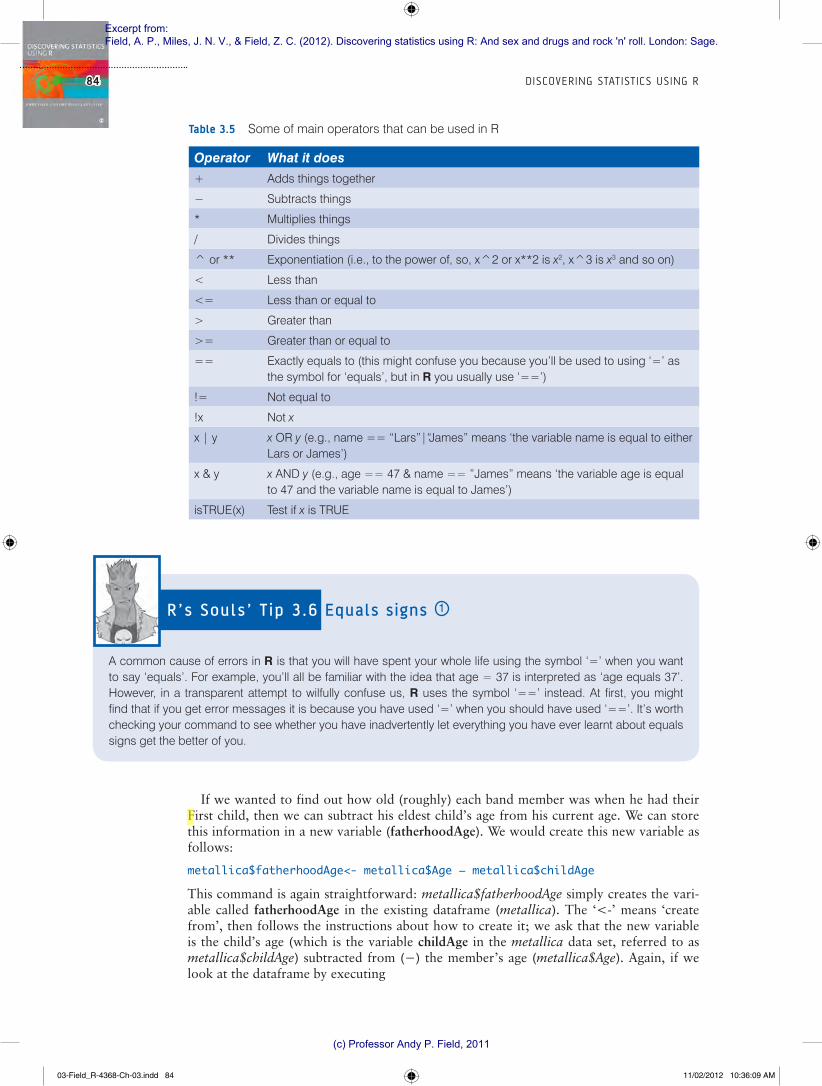
Although we’re not going to get into it too much here (but see Chapter 5), we can also use arithmetic and logical operators to create new variables from existing ones. Table 3.5 overviews some of the basic operators that are used in R. As you can see, there are many operations with which you will be familiar (but see R’s Souls’ Tip 3.6) that you can use on variables: you can add them (using +), subtract them (using #), divide them (using /), and multiply them (using *). We will encounter these and the others in the table as we progress through the book. For now, though, we will look at a simple example to give you a sense that dataframes are versatile frameworks for storing and manipulating data.
R ’s Souls ’ T ip 3 .5 The list() and cbind() functions 1
Dataframes are not the only way to combine variables in R: throughout the book you will find us using the list() and cbind() functions to combine variables. The list() function creates a list of separate objects; you can imagine it as though it is your handbag (or manbag) but nicely organized. Your handbag contains lots of different objects: lipstick, phone, iPod, pen, etc. Those objects can be different, but that doesn’t stop them being collected into the same bag. The list() function creates a sort of bag into which you can place objects that you have created in R. However, it’s a well-organized bag and so objects that you place in it are given a number to indicate whether they are the first, second etc. object in the bag. For example, if we executed these commands:
metallica<-list(metallicaNames, metallicaAges)
instead of the data.frame() function from the chapter, we would create a R-like handbag called metallica that looks like this:
[[1]][1] “Lars” “James” “Kirk” “Rob” [[2]][1] 47 47 48 46
Object [1] in the bag is the list of names, and object [2] in the bag is the list of ages.The function cbind() is used simply for pasting columns of data together (you can also use rbind() to combine
rows of data together). For example, if we execute:
metallica<-cbind(metallicaNames, metallicaAges)
instead of the data.frame() function from the chapter, we would create a matrix called metallica that looks like this:
metallicaNames metallicaAges
[1,] “Lars” “47” [2,] “James” “47” [3,] “Kirk” “48” [4,] “Rob” “46”
Notice that the end result is that the two variables have been pasted together as different columns in the same object. However, notice that the numbers are in quotes; this is because the variable containing names is text, so it causes the ages to be text as well. For this reason, cbind() is most useful for combining variables of the same type.
In general, dataframes are a versatile way to store variables: unlike cbind(), data.frame() stores variables of different types together (trivia note: cbind() works by using the data.frame() function so they’re basically the same). Therefore, we tend to work with dataframes; however, we will use list() sometimes because some functions like to work with lists of variables, and we will sometimes use cbind() as a quick method for combining numeric variables.
03-Field_R-4368-Ch-03.indd 83 11/02/2012 10:36:09 AM
Excerpt from: Field, A. P., Miles, J. N. V., & Field, Z. C. (2012). Discovering statistics using R: And sex and drugs and rock 'n' roll. London: Sage.
(c) Professor Andy P. Field, 2011
84 D ISCOVER ING STAT IST ICS US ING R
If we wanted to find out how old (roughly) each band member was when he had their First child, then we can subtract his eldest child’s age from his current age. We can store this information in a new variable (fatherhoodAge). We would create this new variable as follows:
metallica$fatherhoodAge<- metallica$Age ! metallica$childAge
This command is again straightforward: metallica$fatherhoodAge simply creates the vari-able called fatherhoodAge in the existing dataframe (metallica). The ‘<-’ means ‘create from’, then follows the instructions about how to create it; we ask that the new variable is the child’s age (which is the variable childAge in the metallica data set, referred to as metallica$childAge) subtracted from (!) the member’s age (metallica$Age). Again, if we look at the dataframe by executing
Table 3.5 Some of main operators that can be used in R
Operator What it does+ Adds things together
! Subtracts things
* Multiplies things
/ Divides things
^ or ** Exponentiation (i.e., to the power of, so, x^2 or x**2 is x2, x^3 is x3 and so on)
< Less than
<= Less than or equal to
> Greater than
>= Greater than or equal to
== Exactly equals to (this might confuse you because you’ll be used to using ‘=’ as the symbol for ‘equals’, but in R you usually use ‘==’)
!= Not equal to
!x Not x
x | y x OR y (e.g., name == “Lars”|“James” means ‘the variable name is equal to either Lars or James’)
x & y x AND y (e.g., age == 47 & name == ”James” means ‘the variable age is equal to 47 and the variable name is equal to James’)
isTRUE(x) Test if x is TRUE
R ’s Souls ’ T ip 3 .6 Equals signs 1
A common cause of errors in R is that you will have spent your whole life using the symbol ‘=’ when you want to say ‘equals’. For example, you’ll all be familiar with the idea that age = 37 is interpreted as ‘age equals 37’. However, in a transparent attempt to wilfully confuse us, R uses the symbol ‘==’ instead. At first, you might find that if you get error messages it is because you have used ‘=’ when you should have used ‘==’. It’s worth checking your command to see whether you have inadvertently let everything you have ever learnt about equals signs get the better of you.
03-Field_R-4368-Ch-03.indd 84 11/02/2012 10:36:09 AM
Excerpt from: Field, A. P., Miles, J. N. V., & Field, Z. C. (2012). Discovering statistics using R: And sex and drugs and rock 'n' roll. London: Sage.
(c) Professor Andy P. Field, 2011
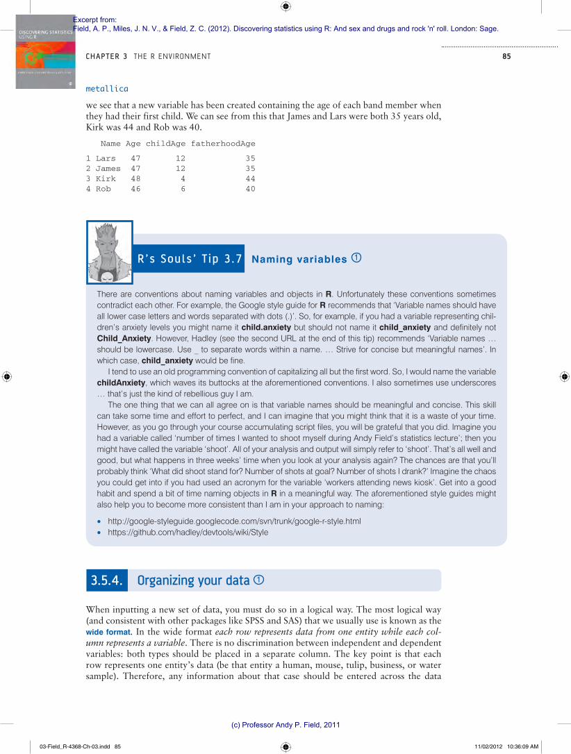
85CHAPTER 3 THE R ENV IRONMENT
metallica
we see that a new variable has been created containing the age of each band member when they had their first child. We can see from this that James and Lars were both 35 years old, Kirk was 44 and Rob was 40.
Name Age childAge fatherhoodAge
1 Lars 47 12 352 James 47 12 353 Kirk 48 4 444 Rob 46 6 40
R ’s Souls ’ T ip 3 .7 Naming variables 1
There are conventions about naming variables and objects in R. Unfortunately these conventions sometimes contradict each other. For example, the Google style guide for R recommends that ‘Variable names should have all lower case letters and words separated with dots (.)’. So, for example, if you had a variable representing chil-dren’s anxiety levels you might name it child.anxiety but should not name it child_anxiety and definitely not Child_Anxiety. However, Hadley (see the second URL at the end of this tip) recommends ‘Variable names … should be lowercase. Use _ to separate words within a name. … Strive for concise but meaningful names’. In which case, child_anxiety would be fine.
I tend to use an old programming convention of capitalizing all but the first word. So, I would name the variable childAnxiety, which waves its buttocks at the aforementioned conventions. I also sometimes use underscores … that’s just the kind of rebellious guy I am.
The one thing that we can all agree on is that variable names should be meaningful and concise. This skill can take some time and effort to perfect, and I can imagine that you might think that it is a waste of your time. However, as you go through your course accumulating script files, you will be grateful that you did. Imagine you had a variable called ‘number of times I wanted to shoot myself during Andy Field’s statistics lecture’; then you might have called the variable ‘shoot’. All of your analysis and output will simply refer to ‘shoot’. That’s all well and good, but what happens in three weeks’ time when you look at your analysis again? The chances are that you’ll probably think ‘What did shoot stand for? Number of shots at goal? Number of shots I drank?’ Imagine the chaos you could get into if you had used an acronym for the variable ‘workers attending news kiosk’. Get into a good habit and spend a bit of time naming objects in R in a meaningful way. The aforementioned style guides might also help you to become more consistent than I am in your approach to naming:
http://google-styleguide.googlecode.com/svn/trunk/google-r-style.html https://github.com/hadley/devtools/wiki/Style
3.5.4. Organizing your data 1
When inputting a new set of data, you must do so in a logical way. The most logical way (and consistent with other packages like SPSS and SAS) that we usually use is known as the wide format. In the wide format each row represents data from one entity while each col-umn represents a variable. There is no discrimination between independent and dependent variables: both types should be placed in a separate column. The key point is that each row represents one entity’s data (be that entity a human, mouse, tulip, business, or water sample). Therefore, any information about that case should be entered across the data
03-Field_R-4368-Ch-03.indd 85 11/02/2012 10:36:09 AM
Excerpt from: Field, A. P., Miles, J. N. V., & Field, Z. C. (2012). Discovering statistics using R: And sex and drugs and rock 'n' roll. London: Sage.
(c) Professor Andy P. Field, 2011
86 D ISCOVER ING STAT IST ICS US ING R
editor. For example, imagine you were interested in sex differences in perceptions of pain created by hot and cold stimuli. You could place some people’s hands in a bucket of very cold water for a minute and ask them to rate how painful they thought the experience was on a scale of 1 to 10. You could then ask them to hold a hot potato and again measure their perception of pain. Imagine I was a participant. You would have a single row representing my data, so there would be a different column for my name, my gender, my pain percep-tion for cold water and my pain perception for a hot potato: Andy, male, 7, 10.
The column with the information about my gender is a grouping variable (also known as a factor): I can belong to either the group of males or the group of females, but not both. As such, this variable is a between-group variable (different entities belong to different groups). Rather than representing groups with words, R uses numbers and words. This involves assigning each group a number, and a label that descibes the group. Therefore, between-group variables are represented by a single column in which the group to which the person belonged is defined using a number and label (see section 3.5.4.3). For example, we might decide that if a person is male then we give them the number 0, and if they’re female we give them the number 1. We then have to tell R that every time it sees a 1 in a particular column the person is a female, and every time it sees a 0 the person is a male. Variables that specify to which of several groups a person belongs can be used to split up data files (so in the pain example you could run an analysis on the male and female partici-pants separately – see section 5.5.3).
Finally, the two measures of pain are a repeated measure (all participants were subjected to hot and cold stimuli). Therefore, levels of this variable (see R’s Souls’ Tip 3.8) can be entered in separate columns (one for pain perception for a hot stimulus and one for pain perception for a cold stimulus).
R ’s Souls ’ T ip 3 .8 Entering data 1
There is a simple rule for how variables are typically arranged in an R dataframe: data from different things go in different rows of the dataframe, whereas data from the same things go in different columns of the dataframe. As such, each person (or mollusc, goat, organization, or whatever you have measured) is represented in a different row. Data within each person (or mollusc, etc.) go in different columns. So, if you’ve prodded your mollusc, or human, several times with a pencil and measured how much it twitches as an outcome, then each prod will be represented by a column.
In experimental research this means that any variable measured with the same participants (a repeated mea-sure) should be represented by several columns (each column representing one level of the repeated-measures variable). However, any variable that defines different groups of things (such as when a between-group design is used and different participants are assigned to different levels of the independent variable) is defined using a single column. This idea will become clearer as you learn about how to carry out specific procedures. (This golden rule is not as golden as it seems at first glance – often data need to be arranged in a different format ! but it’s a good place to start and it’s reasonable easy to rearrange a dataframe – see section 3.9.)
Imagine we were interested in looking at the differences between lecturers and students. We took a random sample of five psychology lecturers from the University of Sussex and five psychology students and then measured how many friends they had, their weekly
03-Field_R-4368-Ch-03.indd 86 11/02/2012 10:36:09 AM
Excerpt from: Field, A. P., Miles, J. N. V., & Field, Z. C. (2012). Discovering statistics using R: And sex and drugs and rock 'n' roll. London: Sage.
(c) Professor Andy P. Field, 2011
87CHAPTER 3 THE R ENV IRONMENT
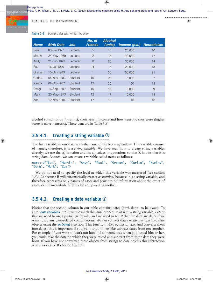
alcohol consumption (in units), their yearly income and how neurotic they were (higher score is more neurotic). These data are in Table 3.6.
3.5.4.1. Creating a string variable 1
The first variable in our data set is the name of the lecturer/student. This variable consists of names; therefore, it is a string variable. We have seen how to create string variables already: we use the c() function and list all values in quotations so that R knows that it is string data. As such, we can create a variable called name as follows:
name<-c("Ben", "Martin", "Andy", "Paul", "Graham", "Carina", "Karina", "Doug", "Mark", "Zoe")
We do not need to specify the level at which this variable was measured (see section 1.5.1.2) because R will automatically treat it as nominal because it is a string variable, and therefore represents only names of cases and provides no information about the order of cases, or the magnitude of one case compared to another.
3.5.4.2. Creating a date variable 1
Notice that the second column in our table contains dates (birth dates, to be exact). To enter date variables into R we use much the same procedure as with a string variable, except that we need to use a particular format, and we need to tell R that the data are dates if we want to do any date-related computations. We can convert dates written as text into date objects using the as.Date() function. This function takes strings of text, and converts them into dates; this is important if you want to do things like subtract dates from one another. For example, if you want to work out how old someone was when you tested him or her, you could take the date on which they were tested and subtract from it the date they were born. If you have not converted these objects from strings to date objects this subtraction won’t work (see R’s Souls’ Tip 3.9).
Table 3.6 Some data with which to play
Name Birth Date JobNo. of
FriendsAlcohol (units) Income (p.a.) Neuroticism
Ben 03-Jul-1977 Lecturer 5 10 20,000 10
Martin 24-May-1969 Lecturer 2 15 40,000 17
Andy 21-Jun-1973 Lecturer 0 20 35,000 14
Paul 16-Jul-1970 Lecturer 4 5 22,000 13
Graham 10-Oct-1949 Lecturer 1 30 50,000 21
Carina 05-Nov-1983 Student 10 25 5,000 7
Karina 08-Oct-1987 Student 12 20 100 13
Doug 16-Sep-1989 Student 15 16 3,000 9
Mark 20-May-1973 Student 12 17 10,000 14
Zoë 12-Nov-1984 Student 17 18 10 13
03-Field_R-4368-Ch-03.indd 87 11/02/2012 10:36:09 AM
Excerpt from: Field, A. P., Miles, J. N. V., & Field, Z. C. (2012). Discovering statistics using R: And sex and drugs and rock 'n' roll. London: Sage.
(c) Professor Andy P. Field, 2011
88 D ISCOVER ING STAT IST ICS US ING R
R ’s Souls ’ T ip 3 .9 Dates 1
If you want to do calculations involving dates then you need to tell R to treat a variable as a date object. Let’s look at what happens if we don’t. Imagine two variables (husband and wife) that contain the birthdates of four men and their respective wives. We might create these variables and enter these birthdates as follows:
husband<-c("1973-06-21", "1970-07-16", "1949-10-08", "1969-05-24")
wife<-c("1984-11-12", "1973-08-02", "1948-11-11", "1983-07-23")
If we want to now calculate the age gap between these partners, then we could create a new variable, agegap, which is the difference between the two variables (husband ! wife):
agegap <- husband-wife
We’d find this rather disappointing message in the console:
Error in husband - wife : non-numeric argument to binary operator
This message is R’s way of saying ‘What the hell are trying to get me to do? These are words; I can’t subtract letters from each other.’
However, if we use the as.Date() function when we create the variables then R knows that the strings of text are dates:
husband<-as.Date(c("1973-06-21", "1970-07-16", "1949-10-08", "1969-05-24"))
wife<-as.Date(c("1984-11-12", "1973-08-02", "1948-11-11", "1983-07-23"))
If we try again to calculate the difference between the two variables:
agegap <- husband-wife
agegap
we get a more sensible output:
Time differences in days
[1] -4162 -1113 331 -5173
This output tells us that in the first couple the wife is 4162 days younger than her husband (about 11 years), for the third couple the wife is 331 days older (just under a year).
The as.Date() function is placed around the function that we would normally use to enter a series of strings. Normally if we enter strings we use the form:
variable<-c("string 1", "string 2", "string 3", etc.)
For dates, these strings need to be in the form yyyy-mm-dd. In other words, if we want to enter the date 21 June 1973, then we would enter it as “1973-06-21”. As such, we could create a variable called birth_date containing the dates of birth by executing the following command:
birth_date<-as.Date(c("1977-07-03", "1969-05-24", "1973-06-21", "1970-07-16", "1949-10-10", "1983-11-05", "1987-10-08", "1989-09-16", "1973-05-20", "1984-11-12"))
Note that we have entered each date as a text string (in quotations) in the appropriate format (yyyy-mm-dd). By enclosing these data in the as.Date() function, these strings are converted to date objects.
03-Field_R-4368-Ch-03.indd 88 11/02/2012 10:36:10 AM
Excerpt from: Field, A. P., Miles, J. N. V., & Field, Z. C. (2012). Discovering statistics using R: And sex and drugs and rock 'n' roll. London: Sage.
(c) Professor Andy P. Field, 2011
89CHAPTER 3 THE R ENV IRONMENT
3.5.4.3. Creating coding variables/factors 1
A coding variable (also known as a grouping variable or factor) is a variable that uses num-bers to represent different groups of data. As such, it is a numeric variable, but these num-bers represent names (i.e., it is a nominal variable). These groups of data could be levels of a treatment variable in an experiment, different groups of people (men or women, an experimental group or a control group, ethnic groups, etc.), different geographic locations, different organizations, etc.
In experiments, coding variables represent independent variables that have been mea-sured between groups (i.e., different participants were assigned to different groups). If you were to run an experiment with one group of participants in an experimental condition and a different group of participants in a control group, you might assign the experimental group a code of 1 and the control group a code of 0. When you come to put the data into R you would create a variable (which you might call group) and type in the value 1 for any participants in the experimental group, and 0 for any participant in the control group. These codes tell R that all of the cases that have been assigned the value 1 should be treated as belonging to the same group, and likewise for the cases assigned the value 0. In situations other than experiments, you might simply use codes to distinguish naturally occurring groups of people (e.g., you might give students a code of 1 and lecturers a code of 0). These codes are completely arbitrary; for the sake of convention people typically use 0, 1, 2, 3, etc., but in practice you could have a code of 495 if you were feeling particularly arbitrary.
We have a coding variable in our data: the one describing whether a person was a lec-turer or student. To create this coding variable, we follow the steps for creating a normal variable, but we also have to tell R that the variable is a coding variable/factor and which numeric codes have been assigned to which groups.
First, we can enter the data and then worry about turning these data into a coding vari-able. In our data we have five lecturers (who we will code with 1) and five students (who we will code with 2). As such, we need to enter a series of 1s and 2s into our new variable, which we’ll call job. The way the data are laid out in Table 3.6 we have the five lecturers followed by the five students, so we can enter the data as:
job<-c(1,1,1,1,1,2,2,2,2,2)
In situations like this, in which all cases in the same group are grouped together in the data file, we could do the same thing more quickly using the rep() function. This function takes the general form of rep(number to repeat, how many repetitions). As such, rep(1, 5) will repeat the number 1 five times. Therefore, we could generate our job variable as follows:
job<-c(rep(1, 5),rep(2, 5))
Whichever method you use the end results is the same:
job
[1] 1 1 1 1 1 2 2 2 2 2
To turn this variable into a factor, we use the factor() function. This function takes the general form:
factor(variable, levels = c(x,y, … z), labels = c("label1", "label2", … "label3"))
This looks a bit scary, but it’s not too bad really. Let’s break it down: factor(variableName) is all you really need to create the factor – in our case factor(job) would do the trick. However, we need to tell R which values we have used to denote different groups and we do this with levels = c(1,2,3,4, …); as usual we use the c() function to list the values we have used. If we have used a regular series such as 1, 2, 3, 4 we can abbreviate this
03-Field_R-4368-Ch-03.indd 89 11/02/2012 10:36:10 AM
Excerpt from: Field, A. P., Miles, J. N. V., & Field, Z. C. (2012). Discovering statistics using R: And sex and drugs and rock 'n' roll. London: Sage.
(c) Professor Andy P. Field, 2011

90 D ISCOVER ING STAT IST ICS US ING R
as c(1:4), where the colon simply means ‘all the values between’; so, c(1:4) is the same as c(1,2,3,4) and c(0:6) is the same as c(0,1,2,3,4,5,6). In our case, we used 1 and 2 to denote the two groups, so we could specify this as c(1:2) or c(1,2). The final step is to assign labels to these levels using labels = c(“label”, …). Again, we use c() to list the labels that we wish to assign. You must list these labels in the same order as your numeric levels, and you need to make sure you have provided a label for each level. In our case, 1 cor-responds to lecturers and 2 to students, so we would want to specify labels of “Lecturer” and “Student”. As such, we could write levels = c(“Lecturers”, “Students”). If we put all of this together we get this command, which we can execute to transform job into a cod-ing variable:
job<-factor(job, levels = c(1:2), labels = c("Lecturer", "Student"))
Having converted job to a factor, R will treat it as a nominal variable. A final way to gener-ate factors is to use the gl() function – the ‘gl’ stands for general (factor) levels. This func-tion takes the general form:
newFactor<-gl(number of levels, cases in each level, total cases, labels = c("label1", "label2"…))
which creates a factor variable called newFactor; you specify the number of levels or groups of the factor, how many cases are in each level/group, optionally the total number of cases (the default is to multiply the number of groups by the number of cases per group), and you can also use the labels option to list names for each level/group. We could generate the variable job as follows:
job<-gl(2, 5, labels = c("Lecturer", "Student"))
The end result is a fully-fledged coding variable (or factor):
[1] Lecturer Lecturer Lecturer Lecturer Lecturer Student Student Student Student Student
With any factor variable you can see the factor levels and their order by using the levels() function, in which you enter the name of the factor. So, to see the levels of our variable job we could execute:
levels(job)
which will produce this output:
[1] “Lecturer” “Student”
In other words, we know that the variable job has two levels and they are (in this order) Lecturer and Student. We can also use this function to set the levels of a variable. For example, imagine we wanted these levels to be called Medical Lecturer and Medical Student, we could execute:
levels(job)<-c("Medical Lecturer", "Medical Student")
This command will rename the levels associated with the variable job (note, the new names are entered as text with speech marks, and are wrapped up in the c() function). You can also use this function to reorder the levels of a factor – see R’s Souls’ Tip 3.13.
This example should clarify why in experimental research grouping variables are used for variables that have been measured between participants: because by using a coding variable it is impossible for a participant to belong to more than one group. This situation should occur in a between-group design (i.e., a participant should not be tested in both the experimental and the control group). However, in repeated-measures designs (within subjects) each participant is tested in every condition and so we would not use this sort of coding variable (because each participant does take part in every experimental condition)
03-Field_R-4368-Ch-03.indd 90 11/02/2012 10:36:10 AM
Excerpt from: Field, A. P., Miles, J. N. V., & Field, Z. C. (2012). Discovering statistics using R: And sex and drugs and rock 'n' roll. London: Sage.
(c) Professor Andy P. Field, 2011

91CHAPTER 3 THE R ENV IRONMENT
3.5.4.4. Creating a numeric variable 1
Numeric variables are the easiest ones to create and we have already created several of these already in this chapter. Our next four variables are friends, alcohol, income and neu-rotic. These are all numeric variables and you can use what you have learnt so far to create them (I hope!).
SELF-TEST
9 Use what you have learnt about creating variables in R to create variables called friends, alcohol, income and neurotic containing the data in Table 3.6.
Hopefully you have tried out the exercise, and if so you should have executed the fol-lowing commands:
friends<-c(5,2,0,4,1,10,12,15,12,17)
alcohol<-c(10,15,20,5,30,25,20,16,17,18)
income<-c(20000,40000,35000,22000,50000,5000,100,3000,10000,10)
neurotic<-c(10,17,14,13,21,7,13,9,14,13)
SELF-TEST
9 Having created the variables in Table 3.6, construct a dataframe containing them all called lecturerData.
Having created the individual variables we can bind these together in a dataframe. We do this by executing this command:
lecturerData<-data.frame(name,birth_date,job,friends,alcohol,income, neurotic)
If we look at the contents of this dataframe you should hopefully see the same as Table 3.6:
> lecturerData
name birth_date job friends alcohol income neurotic1 Ben 1977-07-03 Lecturer 5 10 20000 102 Martin 1969-05-24 Lecturer 2 15 40000 173 Andy 1973-06-21 Lecturer 0 20 35000 144 Paul 1970-07-16 Lecturer 4 5 22000 135 Graham 1949-10-10 Lecturer 1 30 50000 216 Carina 1983-11-05 Student 10 25 5000 77 Karina 1987-10-08 Student 12 20 100 138 Doug 1989-09-16 Student 15 16 3000 99 Mark 1973-05-20 Student 12 17 10000 1410 Zoe 1984-11-12 Student 17 18 10 13
03-Field_R-4368-Ch-03.indd 91 11/02/2012 10:36:11 AM
Excerpt from: Field, A. P., Miles, J. N. V., & Field, Z. C. (2012). Discovering statistics using R: And sex and drugs and rock 'n' roll. London: Sage.
(c) Professor Andy P. Field, 2011

113CHAPTER 3 THE R ENV IRONMENT
R packages used in this chapter
foreign Rcmdr
R functions used in this chapter as.Date()as.matrix()c()cast()choose.file()data.frame()factor()getwd()gl()help()install.packages()levels()library()mean()melt()
names()print()read.csv()read.delim()read.spss()recode()rep()reshape()setwd()stack()subset()unstack()write.csv()write.table()
What have I discovered about statistics? 1
This chapter has provided a basic introduction to the R environment. We’ve seen that R is free software that you can download from the Internet. People with big brains contribute packages that enable you to carry out different tasks in R. They upload these packages to a mystical entity known as the CRAN, and you download them from there into your com-puter. Once you have installed and loaded a package you can use the functions within it.
We also saw that R operates through written commands. When conducting tasks in R, you write commands and then execute them (either in the console window, or using a script file). It was noteworthy that we learned that we cannot simply write “R, can you analyse my data for me please” but actually have to use specific functions and com-mands. Along the way, we discovered that R will do its best to place obstacles in our way: it will pedantically fail to recognize functions and variables if they are not written exactly as they should be, it will spew out vitriolic error messages if we miss punctuation marks, and it will act aloof and uninterested if we specify incorrectly even the smallest detail. It believes this behaviour to be character building.
You also created your first data set by specifying some variables and inputting some data. In doing so you discovered that we can code groups of people using numbers (coding vari-ables) and discovered that rows in the data represent different entities (or cases of data) and columns represent different variables. Unless of course you use the long format, in which case a completely different set of rules apply. That’s OK, though, because we learnt how to transform data from wide to long format. The joy that brought to us can barely be estimated.
We also discovered that I was scared of my new school. However, with the help of Jonathan Land my confidence grew. With this new confidence I began to feel comfort-able not just at school but in the world at large. It was time to explore.
03-Field_R-4368-Ch-03.indd 113 11/02/2012 10:37:42 AM
Excerpt from: Field, A. P., Miles, J. N. V., & Field, Z. C. (2012). Discovering statistics using R: And sex and drugs and rock 'n' roll. London: Sage.
(c) Professor Andy P. Field, 2011