Embed Size (px)
Citation preview

The R package MitISEM: Efficient and robust simulation procedures for Bayesian inference
NORGES BANKRESEARCH
10 | 2017
NALAN BASTURK, STEFANO GRASSI, LENNART HOOGERHEIDE, ANNE OPSCHOOR ANDHERMAN K. VAN DIJK
WORKING PAPER

NORGES BANK
WORKING PAPERXX | 2014
RAPPORTNAVN
2
Working papers fra Norges Bank, fra 1992/1 til 2009/2 kan bestilles over e-post: [email protected]
Fra 1999 og senere er publikasjonene tilgjengelige på www.norges-bank.no Working papers inneholder forskningsarbeider og utredninger som vanligvis ikke har fått sin endelige form. Hensikten er blant annet at forfatteren kan motta kommentarer fra kolleger og andre interesserte. Synspunkter og konklusjoner i arbeidene står for forfatternes regning.
Working papers from Norges Bank, from 1992/1 to 2009/2 can be ordered by e-mail:[email protected]
Working papers from 1999 onwards are available on www.norges-bank.no
Norges Bank’s working papers present research projects and reports (not usually in their final form) and are intended inter alia to enable the author to benefit from the comments of colleagues and other interested parties. Views and conclusions expressed in working papers are the responsibility of the authors alone.
ISSN 1502-819-0 (online) ISBN 978-82-7553-987-6 (online)

The R Package MitISEM: Efficient and Robust
Simulation Procedures for Bayesian Inference∗
Nalan BasturkMaastricht University
& RCEA
Stefano GrassiUniversity of Rome
“Tor Vergata”
Lennart HoogerheideVrije Universiteit Amsterdam
& Tinbergen Institute
Anne OpschoorVrije Universiteit Amsterdam
& Tinbergen Institute
Herman K. van Dijk
Erasmus University Rotterdam
& The Norges Bank
& Tinbergen Institute & RCEA
Abstract
This paper presents the R package MitISEM (mixture of t by importance samplingweighted expectation maximization) which provides an automatic and flexible two-stagemethod to approximate a non-elliptical target density kernel – typically a posterior den-sity kernel – using an adaptive mixture of Student-t densities as approximating density. Inthe first stage a mixture of Student-t densities is fitted to the target using an expectationmaximization algorithm where each step of the optimization procedure is weighted usingimportance sampling. In the second stage this mixture density is a candidate density forefficient and robust application of importance sampling or the Metropolis-Hastings (MH)method to estimate properties of the target distribution. The package enables Bayesianinference and prediction on model parameters and probabilities, in particular, for mod-els where densities have multi-modal or other non-elliptical shapes like curved ridges.These shapes occur in research topics in several scientific fields. For instance, analysisof DNA data in bio-informatics, obtaining loans in the banking sector by heterogeneousgroups in financial economics and analysis of education’s effect on earned income in laboreconomics. The package MitISEM provides also an extended algorithm, ‘sequential Mi-tISEM’, which substantially decreases computation time when the target density has tobe approximated for increasing data samples. This occurs when the posterior or predictivedensity is updated with new observations and/or when one computes model probabilitiesusing predictive likelihoods. We illustrate the MitISEM algorithm using three canonicalstatistical and econometric models that are characterized by several types of non-ellipticalposterior shapes and that describe well-known data patterns in econometrics and finance.We show that MH using the candidate density obtained by MitISEM outperforms, interms of numerical efficiency, MH using a simpler candidate, as well as the Gibbs sam-pler. The MitISEM approach is also used for Bayesian model comparison using predictivelikelihoods.
Keywords: finite mixtures, Student-t densities, importance sampling, MCMC, Metropolis-Hastings algorithm, expectation maximization, Bayesian inference, R software.
∗This paper should not be reported as representing the views of Norges Bank. The views expressed arethose of the authors and do not necessarily reflect those of Norges Bank.

2 The R package MitISEM
1. Introduction
There exist several classes of important statistical and econometric models where posteriorand/or predictive distributions have unknown analytical properties and non-elliptical BayesianHighest Posterior Density (HPD) credible sets. For a theoretical background see e.g., Berger(1985) and as examples we name the class of so-called instrumental variable regression modelswith weak instruments where, for instance, the effect of years of education on income is mod-eled and measured. This is very relevant for government agencies responsible for compulsoryschooling laws. A second example is the class of mixture processes where one component isnearly non-identified since it corresponds to very few observations, which may occur in finan-cial models with data that exhibit time varying volatility patterns and heavy tails and it mayalso occur in epidemiological models with regional data patterns where very few observationsof a disease occur. A detailed analysis of this literature is beyond the scope of the presentpaper. We refer to, e.g., Imbens and Angrist (1994) and Bos, Mahieu, and Van Dijk (2000),the references cited there and to several textbooks: Lancaster (2004); Geweke (2005); Rossi,Allemby, and McCulloch (2005) and Koop, Poirier, and Tobias (2007) for more background.In such studies an important technical issue is the development of efficient and robust proce-dures to generate (pseudo-) random draws from non-elliptical distributions in a numericallyefficient way. Even if simulation from the conditional distributions is relatively easy, for ex-ample, using the well-known Gibbs sampler, multi-modality and/or high correlations betweenmodel parameters may cause this sampler to converge extremely slowly and yield erroneousresults even with a relatively large sample of draws. We illustrate this in the present paper.
Two stage method and the approximation property
This paper presents the R (R Core Team 2017) package MitISEM (Basturk, Hoogerheide, Op-schoor, and Van Dijk 2017) which provides an automatic and flexible method to approximatea target posterior or predictive density by an adaptive mixture of Student-t densities, alsoreferred to in the following as approximate, candidate or proposal density1. The multivariatetarget density can be non-elliptical like being multi-modal, strongly correlated and/or havingcurved ridges in the surface. Only a kernel of the target density is required for the MitISEMmethod, which is typically a posterior density kernel. Our method consists of two stages.In the first stage a mixture of Student-t candidate densities is fitted to the target using anexpectation maximization (EM) algorithm where each step of the optimization procedure isweighted using importance sampling. Details are given in Section 2. In the second stage theobtained candidate density can be used in importance sampling or the independence chainMetropolis-Hastings method for Bayesian inference on model parameters and model proba-bilities. The MitISEM method has been introduced by Hoogerheide, Opschoor, and Van Dijk(2012) and it has been shown that the method provides substantial gains in computationalefficiency in Bayesian estimation. The MitISEM method makes use of convex combinations ofdensities, and the approximation properties of such density combinations have been analyzedextensively in the literature. For instance Zeevi and Meir (1997) show that under certainconditions any density function may be approximated to arbitrary accuracy by a convex com-bination of ‘basis’ densities. The class of mixtures of Student-t densities falls within thisframework.
Algorithmic steps
In the first stage the algorithm MitISEM iterates over importance weighted expectation max-
1These three terms are interchangeably used in the literature and we also do that in the present paper.

Nalan Basturk, Lennart Hoogerheide, Anne Opschoor, Herman K. van Dijk 3
imization steps in order to efficiently construct a mixture of Student-t densities that is anaccurate approximation of the target density. Starting with a single Student-t density, newmixture components are added in an iterative way until the required approximation is reached.At each iteration, parameters of the mixture components – consisting of mode, scale, degreesof freedom and mixing probability – are optimized such that the Kullback-Leibler divergencebetween target density and candidate density of Student-t mixtures is minimized. The con-structed mixture is used in the second stage for efficient and robust application of eitherimportance sampling (IS) or the independence chain Metropolis-Hastings (MH) method.
Illustrations
We illustrate the MitISEM algorithm using a well-known statistical example distribution fromGelman and Meng (1991) that is characterized by a very non-elliptical, possibly bi-modal,joint distribution while the conditional distributions are normal. We also use the posteriordistributions in two classes of canonical econometric models: the generalized autoregressiveconditional heteroskedasticity (GARCH) model that is extensively used in financial econo-metrics and the Instrumental Variable (IV) regression model that is often used to study theeffect of number of years of education on earned income. Both classes of models yield non-elliptical posterior and/or predictive distributions. Furthermore, we show that the MitISEMapproach can be used for the evaluation of model probabilities from predictive likelihoods,which are useful for Bayesian model comparison and model averaging. We also introduce anR program for an adapted MitISEM algorithm as in Hoogerheide, Opschoor, and Van Dijk(2012), named ‘sequential MitISEM’, which substantially decreases the computational timerequired for the candidate density optimization, when the posterior distribution is updatedusing new observations or when one computes model probabilities with predictive likelihoods.
The remainder of this paper is organized as follows: Section 2 discusses the basic idea of theMitISEM method and the ‘sequential MitISEM’ extension, and summarizes the steps of theexpectation maximization algorithm that we make use of. Section 3 presents applications ofthe algorithm to several model structures and datasets. Section 4 concludes.
2. Searching for a mixture of Student-t candidate densitiesusing IS weighted EM
The mixture of Student-t densities that is obtained by making use of importance samplingweighted expectation maximization is based on iteratively adding Student-t densities to themixture (Hoogerheide, Opschoor, and Van Dijk 2012). The algorithm provides an automaticand flexible method to construct a candidate density minimizing the Kullback-Leibler di-vergence (or cross-entropy distance) (Kullback and Leibler 1951) between two densities: theso-called target density, typically a posterior density, and the approximate or candidate den-sity. Each new Student-t component in the candidate density covers the areas of the targetdensity that are not well covered by the previous candidate density. The modes, scales, de-grees of freedom and mixing probabilities are quickly optimized using the importance samplingweighted expectation maximization method.
Henceforth we use the notation f(θ) for the target density kernel of θ, the k-dimensional vectorof interest. f(θ) can be a posterior density kernel of model parameters defined as f(θ|y) fordata y and model parameters θ. Alternatively, f(θ) can be a density kernel f(θ|α) for dataθ and given fixed model parameters α. We concentrate on the former case, where f(θ) is a
4 The R package MitISEM
posterior density kernel, and simplify the notation by having removed the conditioning ondata. Let g(θ) be a candidate density, a mixture of H Student-t densities such that:
g(θ) = g(θ|ζ) =H∑h=1
ηh tk(θ|µh,Σh, νh), (1)
where ζ is the set of location parameters µh, scale matrices Σh, degrees of freedom νh, andmixing probabilities ηh (h = 1, . . . ,H) of the k-dimensional Student-t components with den-sity:
tk(θ|µh,Σh, νh) =Γ(νh+k
2
)Γ(νh
2
)(πνh)k/2
|Σh|−1/2(
1 +(θ − µh)>Σ−1h (θ − µh)
νh
)−(k+νh)/2(2)
with h = 1, . . . ,H and Σh is positive definite, ηh ≥ 0 and∑Hh=1 ηh = 1. We further restrict
νh such that νh ≥ 0.01. Lower and upper bounds for the degrees of freedom parameter νhcan be defined using an optional input to the function MitISEM (e.g., demanding νh > 2).
MitISEM is a new approach that may be compared with the AdMit method (Hoogerheide,Kaashoek, and Van Dijk 2007b), implemented in Ardia, Hoogerheide, and Van Dijk (2009,2017). Both methods rely on the iterative construction of a mixture of Student-t densities asthe candidate density, but there are three substantial differences between these methods.
First, MitISEM minimizes the Kullback-Leibler divergence between target and candidatedensities, while AdMit aims at minimizing the variance of the IS estimator, or the varianceof the IS weights.
Second, in MitISEM all mixture parameters are optimized jointly by means of the relativelyquick EM algorithm, while in the AdMit method means and scale matrices of the candidatecomponents are chosen heuristically and are never updated when additional components areadded to the mixture. That is, AdMit optimizes only mixture component weights. MitISEMimplies a large reduction of the computing time in the approximation procedure, and isexpected to lead to a better candidate in most applications. Therefore the MitISEM methodmay be considered to be a substitute for the AdMit method, rather than an accompanyingmethod.
Third, as shown in Hoogerheide, Opschoor, and Van Dijk (2012), AdMit requires the joint tar-get density kernel, whereas MitISEM requires only candidate draws and importance weights.This implies that AdMit can not be applied partially to the marginal and conditional posteriordensities of subsets of parameters, whereas MitISEM can be used to approximate a marginaldensity of which no kernel is explicitly available.
2.1. Background on importance sampling
Importance sampling (Hammersley and Handscomb 1975; Kloek and Van Dijk 1978) is ageneral method for estimating expectations of a function h(θ) of parameter θ where the prob-ability density function of θ is possibly non-standard. Given a density kernel f(θ) for θ, whereone cannot directly generate random draws from in an easy manner, importance sampling isbased on draws from a different density, the so-called candidate or importance density g(θ),which is easy to simulate from and which is a reasonable approximation to f(θ). Given thisindirect sampling, instead of direct sampling from f(θ), one needs a correction step. That

Nalan Basturk, Lennart Hoogerheide, Anne Opschoor, Herman K. van Dijk 5
is, the draws from the candidate density are weighted according to the importance sampling(IS) weights that are ratios of target over candidate density. For a consistent estimator ofthe expectation of the function of θ, E(h(θ)), the candidate should cover the whole domainof θ values with f(θ) > 0 and the variance of the weights should be bounded (Geweke 1989).The finite sample accuracy of the estimator improves if g(θ) is a good approximation to thetarget kernel (Van Dijk 1984; Van Dijk, Hop, and Louter 1987; Geweke 1989; Hop and VanDijk 1992). IS weights for parameter draws θ from g(θ) are calculated as:
W (θ) = f(θ)/g(θ), (3)
i.e., draws with highest IS weights correspond to the region of the target where the candidateis much smaller than the target and this is a region that is covered too little by the candidatedensity.
Parallel Processing of Computations
Cappe, Douc, Guillin, Marin, and Robert (2008) note that there is a renewed interest inimportance sampling, due to the possibility of parallel processing implementation. Numericalefficiency in sampling methods is not only related to the efficient sample size or relativenumerical efficiency, but also to the possibility to perform the simulation process in a parallelfashion. Unlike alternative methods such as the random walk Metropolis method or the Gibbssampler, importance sampling makes use of independent draws from the candidate density,which in turn can be obtained from multiple core machines or computer clusters. See Gewekeand Durham (2011) for a very novel approach. We are currently exploring the idea to makeuse of paralleled computing in MitISEM. We comment on this possibility in Section 4.
2.2. Background on expectation maximization and our use of this algorithm
The EM algorithm is a method (Dempster, Laird, and Rubin 1977) to achieve the maximumlikelihood estimates of parameters θ in models with incomplete data or latent variables. Anexample of the latter case is the finite mixture model. For the use of the EM algorithm onfinite mixture models, we refer to e.g., McLachlan and Peel (2000); McLachlan and Krishnan(2008).
If the latent variables would be observable, the computation of the maximum likelihood es-timate of θ would be relatively straightforward, depending on the degree of nonlinearity ofthe first order conditions. The idea behind EM is to take the expectation of the objectivefunction, in most cases the log-likelihood function, with respect to the latent variables. Theexpectation of the log-likelihood function is then maximized with respect to the model param-eters. In most models, expectations of the latent variables depend on the model parametersθ, hence the two steps are repeated until convergence.
We emphasize that during the first stage of the method (in which the candidate density isoptimized) we do not have draws from the posterior but instead have draws from a previouslychosen candidate and corresponding importance weights. As a consequence, we make use ofan importance weighted EM algorithm. As shown in Hoogerheide, Opschoor, and Van Dijk(2012), in the MitISEM approach, we minimize the estimated Kullback-Leibler divergence,which implies that we maximize the weighted average of the logarithm of the candidate densityg(.|ζ) evaluated at a set of draws θi from a previous candidate g0(θ), where each candidatevalue log g(θi|ζ) is weighted by the importance sampling weights W i ≡ f(θi)/g0(θ
i) of each

6 The R package MitISEM
draw θi from the previous candidate g0(θ):
1
N
N∑i=1
W i log g(θi|ζ)
where g(.|ζ) is the mixture of Student-t densities to be optimally chosen.
The mixture of Student-t densities (1) for θi is equivalent with the specification
θi ∼ N(µh, wihΣh) if zih = 1,
where zi is a latent H-dimensional vector indicating from which Student-t component the‘observation’ θi stems: if θi stems from component h, then zih = 1, zij = 0 for j 6= h; Pr[zi =
eh] = ηh with eh the h-th column of the identity matrix; wih has the Inverse-Gamma densityIG(νh/2, νh/2). For a more extensive explanation of this mixture of Student-t densities, seee.g., Peel and McLachlan (2000).
2.3. The IS weighted EM algorithm
We reemphasize that in the literature the EM algorithm is typically used to find the optimalvalues of model parameters that maximize the log-likelihood for a given set of data. Here wemake use of EM to find the optimal mixture of Student-t densities for a given set of drawsfrom a previous candidate (and their corresponding weights). We apply an IS-weighted EMalgorithm to these candidate draws instead of a regular EM algorithm to posterior draws(obtained by applying the Metropolis-Hastings method to these candidate draws), since theformer has three advantages. First, we do not require a burn-in sample. Second, the use ofall candidate draws (without the rejections of the MH method) helps to prevent numericalproblems with estimating scale matrices of Student-t components; also draws with relativelysmall, but positive importance weights are helpful for this purpose. Third, the use of allcandidate draws may lead to a better approximation.
In Hoogerheide, Opschoor, and Van Dijk (2012) the different steps of the IS-weighted EMalgorithm in our case are derived. Here we summarize the steps for the mixture of Student-tdensities. Note that when one substitutes for the weight W i the value W i = 1 in Equations 8–10, then one is back in the case of a regular EM algorithm (without IS weighting). In ourcase the L-th expectation step for the mixture of Student-t densities is specified as follows:
zih ≡ E[zih
∣∣∣θi, ζ = ζ(L−1)]
=tk(θ
i|µh,Σh, νh) ηh∑Hj=1 tk(θ
i|µj ,Σj , νj) ηj, (4)
z/wi
h ≡ E
[zihwih
∣∣∣∣∣ θi, ζ = ζ(L−1)]
= zihk + νhρih + νh
, (5)
ξih ≡ E[logwih
∣∣∣θi, ζ = ζ(L−1)]
=
=
[log
(ρih + νh
2
)− ψ
(k + νh
2
)]zih +
[log
(νh2
)− ψ
(νh2
)](1− zih), (6)
δih ≡ E
[1
wih
∣∣∣∣∣ θi, ζ = ζ(L−1)]
=k + νhρih + νh
zih + (1− zih), (7)

Nalan Basturk, Lennart Hoogerheide, Anne Opschoor, Herman K. van Dijk 7
with ρih ≡ (θi−µh)>Σ−1h (θi−µh), ψ(.) the digamma function (the derivative of the logarithmof the gamma function log Γ(.)), and all parameters µh,Σh, νh, ηh elements of the set of can-didate’s parameters ζ(L−1) optimized in the previous EM step (L−1). Given the expectationof the latent variables in Equation 4 to Equation 7, parameters of each mixture componentare updated using the first order conditions of the expectation of the objective function inthe maximization step:
µ(L)h =
[N∑i=1
W i z/wi
h
]−1 [ N∑i=1
W i z/wi
h θi
], (8)
Σ(L)h =
∑Ni=1W
i z/wi
h (θi − µ(L)h )(θi − µ(L)h )>∑Ni=1W
i zih, (9)
η(L)h =
∑Ni=1W
i zih∑Ni=1W
i. (10)
Further, ν(L)h is solved from the first order condition of νh:
−ψ(νh/2) + log(νh/2) + 1−∑Ni=1W
i ξih∑Ni=1W
i−∑Ni=1W
i δih∑Ni=1W
i= 0. (11)
Cappe et al. (2008) only update the expectations and scale structures of the Student-t densi-ties and not the degrees of freedom, because there is no closed-form solution for the latter. Wedo optimize the degrees of freedom parameter νh during the EM procedure to obtain a betterapproximation of the target density. Furthermore, the resulting values of νh (h = 1, . . . ,H)may provide information on the shape, e.g., kurtosis of the target distribution.
2.4. MitISEM: The basic algorithm
Algorithm 1. The MitISEM approach for obtaining an approximation to a target density:
(0) Initialization: Simulate draws θ1, . . . , θN from a ‘naive’ candidate distribution withdensity gnaive, which is obtained as follows. First, we simulate candidate draws from aStudent-t distribution with density gmode, where the mode is taken equal to the modeof the target density and scale matrix equal to minus the inverse Hessian of the log-target density (evaluated at the mode), and where the degrees of freedom are chosen bythe user. Second, the mode and scale of gmode are updated using the IS weighted EMalgorithm. Note that gnaive is already a more advanced candidate than the commonlyused gmode; gmode typically yields a substantially worse numerical efficiency than gnaive.
(1) Adaptation: Estimate the target distribution’s mean and covariance matrix using ISwith the draws θ1, . . . , θN from gnaive. Use these estimates as the mode and scale matrixof Student-t density gadaptive. Draw a sample θ1, . . . , θN from this adaptive Student-tdistribution with density g0 = gadaptive, and compute the IS weights for this sample.
(2) Apply the IS-weighted EM algorithm given the latest IS weights and the drawnsample of step (1). The output consists of the new candidate density g with optimizedζ, the set of µh,Σh, νh, ηh (h = 1, . . . ,H). Draw a new sample θ1, . . . , θN from the

8 The R package MitISEM
distribution that corresponds with this proposal density and compute corresponding ISweights.
(3) Iterate on the number of mixture components: Given the current mixture of Hcomponents with corresponding µh,Σh, νh and ηh (h = 1, . . . ,H), take x% of the sampleθ1, . . . , θN that correspond to the highest IS weights. Construct with these draws andIS weights a new mode µH+1 and scale matrix ΣH+1 which are starting values for theadditional component in the mixture candidate density. This choice ensures that thenew component covers a region of the parameter space in which the previous candidatemixture had relatively too little probability mass. Given the latest IS weights and thedrawn sample from the current mixture of H components, apply the IS-weighted EMalgorithm to optimize each mixture component µh,Σh, νh and ηh with h = 1, . . . ,H+1.Draw a new sample from the mixture of H + 1 components and compute correspondingIS weights.
(4) Assess convergence of the candidate density’s quality by inspecting the ISweights and return to step (3) unless the algorithm has converged.
In step (0), we have specified a novel robustification by updating the initial proposal densityusing an IS weighted EM step compared to the MitISEM algorithm proposed in Hoogerheideet al. (2012). This step improves the algorithm when the initial mode and Hessian estimationin step (0) is poor. If these initial mode and Hessian estimates are obtained by grid-searchalgorithms, the estimates can be poor due to local maxima issues in the target density. Inaddition, first component of the candidate density can be user-specified, e.g., using anotheroptimization algorithm as discussed in Ardia et al. (2009), and the accuracy of these opti-mization algorithms depend on the target density properties. The additional robustificationstep we define eliminates extreme dependence of results to user-specified values especially incase these user-specified values are not accurate.
Step (1) can be seen as an intermediate step which quickly tries to improve the initial candidatedensity g0. If during the EM algorithm, a scale matrix Σh of a Student-t component becomes(nearly) singular, then this h-th component is removed from the mixture. Also if during theEM algorithm, a weight ηh becomes very small, then this h-th component is removed fromthe mixture.
In step (4) convergence can be assessed by computing the relative change in Coefficient ofVariation (CoV) of the IS weights, i.e. the standard deviation of the IS weights divided bytheir mean, as in Hoogerheide, Opschoor, and Van Dijk (2012), who use the candidate fromMitISEM for importance sampling or the independence chain MH method. Zellner, Ando,Basturk, Hoogerheide, and Van Dijk (2014), who use the MitISEM candidate for rejectionsampling, propose an alternative criterion for the convergence of the MitISEM algorithm.They use the unconditional acceptance probability, which is a more natural and intuitiveconvergence criterion in this case of rejection sampling. The default convergence in MitISEM isdefined as the change of the CoV being smaller than 10%, but the user can specify convergencein terms of the acceptance probability. The convergence tolerance can also be altered by theuser.
Starting values for νH+1 and ηH+1 are at each iteration set at 1 and 0.10, respectively. Thatis, the new component has fat tails, and a relatively low probability ex-ante. Starting valuesfor µh, Σh, and νh (h = 1, . . . ,H) are the optimal values in the previous mixture of H

Nalan Basturk, Lennart Hoogerheide, Anne Opschoor, Herman K. van Dijk 9
components, while ηh (h = 1, . . . ,H) is 0.90 times the previously optimal value. Alternativeinitial values for ηH+1 and νH+1 can be set by the user.
Finally, we introduce another novel robustification of the MitISEM method. With this robus-tification, the given number of candidate draws that is used to construct the candidate doesnot include draws for which the target density kernel is 0 (i.e., draws outside the ‘allowed’parameter region). If the target density is concentrated in a restricted parameter space, forexample for a mixture GARCH model, the number of ‘useful’ or ‘effective’ draws can be oth-erwise very small, especially during the first steps of the MitISEM algorithm. This robustsimulation is the default simulation method in the provided package, but can be disregardedby the user.
Approximating the Gelman-Meng density using MitISEM
We illustrate the MitISEM approach using a non-elliptical, bivariate density function proposedby Gelman and Meng (1991). The target density kernel is:
f (x1, x2) = exp{−0.5
(Ax21 + x21 + x22 − 2Bx1x2 − 2C1x1 − 2C2x2
)}, (12)
where (x1, x2)> plays the role of the vector of interest θ.
In order to obtain the MitISEM approximation to the density f(x1, x2) one first defines thetarget density kernel (see also Ardia, Hoogerheide, and Van Dijk (2017)):
R> GelmanMeng <- function(x, A = 1, B = 0, C1 = 3, C2 = 3, log = TRUE){
+ if (is.vector(x))
+ x <- matrix(x, nrow = 1)
+ r <- -0.5 * (A * x[,1]^2 * x[,2]^2 + x[,1]^2 + x[,2]^2
+ - 2 * B * x[,1] * x[,2] - 2 * C1 * x[,1] - 2 * C2 * x[,2])
+ if (!log)
+ r <- exp(r)
+ as.vector(r)
+ }
where an input log is added in this function for the following reason. We evaluate the ISweights in the following way. First, we compute the logarithm IS of the weight (log(W i))as the logarithm of the target density kernel minus the logarithm of the candidate density.Second, we subtract the maximum of the log(W i). Third, we take the exponent to obtainW i. If we would directly evaluate the IS weight as the ratio of the target density kerneland candidate density, then there would often be numerical problems (in the sense of an‘underflow’ or ‘overflow’, where all IS weights are stored as 0 or ∞). Note that rescalingthe IS weights does not matter in Equations 8–11, as W i always occurs in both a numeratorand a denominator of a ratio. So rescaling the IS weights does not matter for the MitISEMalgorithm. Obviously, the scale does matter for the evaluation of marginal and predictivelikelihoods. In these procedures we do keep track of the scale when rescaling. On the otherhand, we may want to plot the target density and the MitISEM approximation. In that casewe want to plot the actual densities, not their logarithm. Therefore, the ‘log’ argument isoptional.
MitISEM approximation to the target kernel is obtained using function MitISEM and an initialpoint, mu0, for the optimization in step (0), where with each additional mixture component,
10 The R package MitISEM
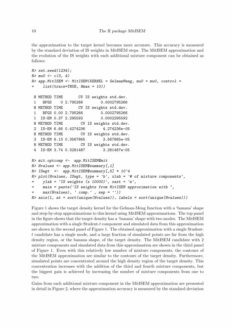
the approximation to the target kernel becomes more accurate. This accuracy is measuredby the standard deviation of IS weights in MitISEM steps. The MitISEM approximation andthe evolution of the IS weights with each additional mixture component can be obtained asfollows:
R> set.seed(1234);
R> mu0 <- c(3, 4)
R> app.MitISEM <- MitISEM(KERNEL = GelmanMeng, mu0 = mu0, control =
+ list(trace=TRUE, Hmax = 10))
H METHOD TIME CV IS weights std.dev.
1 BFGS 0 2.795266 0.0002795266
H METHOD TIME CV IS weights std.dev.
1 BFGS 0.00 2.795266 0.0002795266
1 IS-EM 0.37 2.295592 0.0002295592
H METHOD TIME CV IS weights std.dev.
2 IS-EM 6.66 0.4274236 4.274236e-05
H METHOD TIME CV IS weights std.dev.
3 IS-EM 6.13 0.3567865 3.567865e-05
H METHOD TIME CV IS weights std.dev.
4 IS-EM 3.74 0.3281487 3.281487e-05
R> mit.optcomp <- app.MitISEM$mit
R> Hvalues <- app.MitISEM$summary[,1]
R> ISwgt <- app.MitISEM$summary[,5] * 10^4
R> plot(Hvalues, ISwgt, type = 'b', xlab = '# of mixture components',
+ ylab = 'IS weights (x 10000)', xaxt = 'n',
+ main = paste('IS weights from MitISEM approximation with ',
+ max(Hvalues), ' comp.' , sep = ''))
R> axis(1, at = sort(unique(Hvalues)), labels = sort(unique(Hvalues)))
Figure 1 shows the target density kernel for the Gelman-Meng function with a ‘banana’ shapeand step-by-step approximations to this kernel using MitISEM approximations. The top panelin the figure shows that the target density has a ‘banana’ shape with two modes. The MitISEMapproximation with a single Student-t component and simulated data from this approximationare shown in the second panel of Figure 1. The obtained approximation with a single Student-t candidate has a single mode, and a large fraction of simulated points are far from the highdensity region, or the banana shape, of the target density. The MitISEM candidate with 2mixture components and simulated data from this approximation are shown in the third panelof Figure 1. Even with this relatively low number of mixture components, the contours ofthe MitISEM approximation are similar to the contours of the target density. Furthermore,simulated points are concentrated around the high density region of the target density. Thisconcentration increases with the addition of the third and fourth mixture components, butthe biggest gain is achieved by increasing the number of mixture components from one totwo.
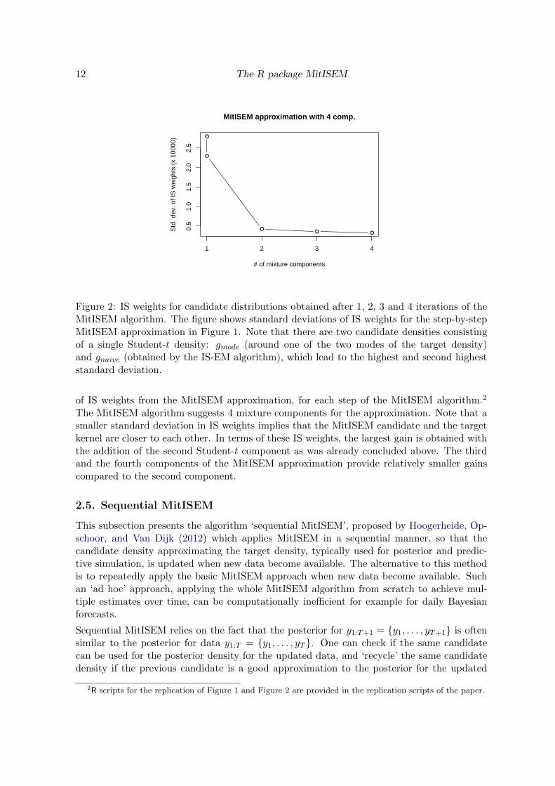
Gains from each additional mixture component in the MitISEM approximation are presentedin detail in Figure 2, where the approximation accuracy is measured by the standard deviation

Nalan Basturk, Lennart Hoogerheide, Anne Opschoor, Herman K. van Dijk 11
target density kernel
x1x 2
−2 0 2 4 6
−2
02
46
MitISEM approximation with 1 comp.
x1
x 2
−2 0 2 4 6
−2
02
46
−2 0 2 4 6−
20
24
6
draws from MitISEM approximation with 1 comp.
x1
x 2
w < q(0.1)q(0.1)<=w <q(0.5)w >=q (0.5)
MitISEM approximation with 2 comp.
x1
x 2
−2 0 2 4 6
−2
02
46
−2 0 2 4 6
−2
02
46
draws from MitISEM approximation with 2 comp.
x1
x 2
w < q(0.1)q(0.1)<=w <q(0.5)w >=q (0.5)
MitISEM approximation with 3 comp.
x1
x 2
−2 0 2 4 6
−2
02
46
−2 0 2 4 6
−2
02
46
draws from MitISEM approximation with 3 comp.
x1
x 2
w < q(0.1)q(0.1)<=w <q(0.5)w >=q (0.5)
MitISEM approximation with 4 comp.
x1
x 2
−2 0 2 4 6
−2
02
46
−2 0 2 4 6
−2
02
46
draws from MitISEM approximation with 4 comp.
x1
x 2
w < q(0.1)q(0.1)<=w <q(0.5)w >=q (0.5)
Figure 1: Evolution of the MitISEM candidate for the Gelman-Meng target density with abanana shape. The figure shows the target density kernel (top panel), the MitISEM approxi-mation to the target density kernel, and draws from this approximation for the Gelman-Mengdensity with a banana shape in Section 3.1, for MitISEM approximation with one to fourStudent-t components. MitISEM approximations are obtained using 105 draws, and 5× 10³
draws from the approximations are plotted. For draws from MitISEM approximations, wdenotes the IS weights of draws where weights are normalized to have mean 1. q(x) denotesthe x× 100 percentage quantile of IS weights from all draws.
12 The R package MitISEM
●
●
●● ●
0.5
1.0
1.5
2.0
2.5
MitISEM approximation with 4 comp.
# of mixture components
Std
. dev
. of I
S w
eigh
ts (
x 10
000)
1 2 3 4
Figure 2: IS weights for candidate distributions obtained after 1, 2, 3 and 4 iterations of theMitISEM algorithm. The figure shows standard deviations of IS weights for the step-by-stepMitISEM approximation in Figure 1. Note that there are two candidate densities consistingof a single Student-t density: gmode (around one of the two modes of the target density)and gnaive (obtained by the IS-EM algorithm), which lead to the highest and second higheststandard deviation.
of IS weights from the MitISEM approximation, for each step of the MitISEM algorithm.2
The MitISEM algorithm suggests 4 mixture components for the approximation. Note that asmaller standard deviation in IS weights implies that the MitISEM candidate and the targetkernel are closer to each other. In terms of these IS weights, the largest gain is obtained withthe addition of the second Student-t component as was already concluded above. The thirdand the fourth components of the MitISEM approximation provide relatively smaller gainscompared to the second component.
2.5. Sequential MitISEM
This subsection presents the algorithm ‘sequential MitISEM’, proposed by Hoogerheide, Op-schoor, and Van Dijk (2012) which applies MitISEM in a sequential manner, so that thecandidate density approximating the target density, typically used for posterior and predic-tive simulation, is updated when new data become available. The alternative to this methodis to repeatedly apply the basic MitISEM approach when new data become available. Suchan ‘ad hoc’ approach, applying the whole MitISEM algorithm from scratch to achieve mul-tiple estimates over time, can be computationally inefficient for example for daily Bayesianforecasts.
Sequential MitISEM relies on the fact that the posterior for y1:T+1 = {y1, . . . , yT+1} is oftensimilar to the posterior for data y1:T = {y1, . . . , yT }. One can check if the same candidatecan be used for the posterior density for the updated data, and ‘recycle’ the same candidatedensity if the previous candidate is a good approximation to the posterior for the updated
2R scripts for the replication of Figure 1 and Figure 2 are provided in the replication scripts of the paper.

Nalan Basturk, Lennart Hoogerheide, Anne Opschoor, Herman K. van Dijk 13
data. Even if the ‘old’ candidate is not a good approximation to the posterior for the updateddata, it may suffice to perform an update using the IS-weighted EM algorithm, keeping thenumber H of Student-t components the same. If the resulting quality is still below a desiredlevel, then one can start the MitISEM algorithm for the updated data, adding componentsuntil convergence. Note that the IS-weighted EM algorithm of MitISEM is much more suitedto perform (either small or large) adaptations than the AdMit method, since in the MitISEMmethod all Student-t components are updated.
Suppose that the MitISEM candidate is optimized for the data until time T and the data setnow includes observations upto time T + τ (τ = 1, 2, . . .). Define y1:T+τ = {y1, . . . , yT+τ}.For the updated data until T + τ the sequential MitISEM steps are as follows:
Algorithm 2. The sequential MitISEM approach for obtaining a candidate density for theposterior density for data y1:T+τ :
(1) Compute CoVrT+τ , the CoV value (Coefficient of Variation of the IS weights) that is
based on the posterior density kernel for data y1:T+τ and the current, reused candidatedensity.
(2) Compare CoVrT+τ with CoVT , the CoV value for the same candidate and the posterior
for data y1:T (the data set at the last time when the candidate was updated). If thechange is below a certain threshold (10%), stop. Otherwise go to step (3).
(3) Run the IS-weighted EM algorithm with the current mixture of H Student-t densities asstarting values. Sample from the new distribution (with the same number of componentsH) and compute IS weights and the corresponding CoVu
T+τ , the CoV value with onlyan EM update. Since the IS-weighted EM algorithm updates all mixture components,it can easily perform a useful shift of the candidate density.
(4) Compare CoVuT+τ and CoVr
T+τ . If the change of quality is below a certain threshold(10%), stop. Otherwise go to step (5).
(5) Iterate on the number of components until the CoV value has converged.
Note that the change in CoV value can be substantial if the new observation yT+1 is an outlier.Steps (3) and (5) in that case will typically be required. A Student-t component is deletedfrom the mixture if the weight of this component is too small, i.e., if the probability of onecomponent is close to zero. The default tolerance for the required mixing probability is 0, anda mixture component is removed from the MitISEM approximation if it has a 0 probability.Hence the number of Student-t components is not necessarily monotonically increasing overtime. This criterion for the removal of a mixture component can be altered by the userthrough an optional input to the function MitISEM. Further, in step (2) CoVr
T+τ is comparedwith CoVT rather than the CoV for the posterior at time yT+τ−1, since in the latter case aseries of small increases of the CoV may eventually lead to a much worse candidate density.
3. Applications in three domains

14 The R package MitISEM
In the following subsections, we make use of the MitISEM and the sequential MitISEM meth-ods in order to deal with distributions that have non-elliptical density contours in threedomains of applications:
(i) Approximating a specific class of well-known, non-elliptical densities in Section 3.1.Here, we continue to analyze the conditionally normal density of Gelman and Meng(1991), which can have non-elliptical, and even distinctly bi-modal, shapes in the jointdensity depending on specific values of the density function parameters. Note that thisis not a posterior density.
(ii) Approximating posterior densities of a class of models popular in financial econometricsin Section 3.2. We consider a standard GARCH model and a mixture GARCH model(for S&P 500 data), which are classes of models extensively used in financial practice. Wefurther consider an instrumental variables (IV) model and compare the approximationperformance using MitISEM candidate with the griddy Gibbs sampler in Ritter andTanner (1992).
(iii) Approximating model probabilities using the concept of predictive likelihoods in Sec-tion 3.3. We consider a mixture GARCH model and an IV model. The latter one usingincome-education data. Both GARCH and IV models yield non-elliptical distributionsfor posterior and predictive densities.
For cases (ii) and (iii) obtaining a good candidate density, for example for importance samplingor the independence chain Metropolis-Hastings method, is crucial for Bayesian estimation ofthe model parameters as well as model probabilities.
For all cases, we summarize the application of the R package MitISEM, and compare theperformance of the MitISEM method with a single, relatively ‘naive’ Student-t candidatedensity. The ‘naive’ density is still an adapted density, obtained by the IS weighted EMalgorithm, with degrees of freedom set as 1. The fat tails of the ‘naive’ candidate density(due to the low degrees of freedom parameter 1) reduce the probability that relevant parts ofthe target density are not covered by the ‘naive’ candidate. Still, despite the optimized modeand scale, this density is expected to lead to a relatively poor approximation in particularfor multi-modal target densities. In Section 3.2.2, we also compare the MitISEM methodwith the AdMit method implemented in Ardia et al. (2017), which also aims to constructa candidate density as a mixture of Student-t densities, in terms of approximation accuracyand computing time.
3.1. Approximating densities: The Gelman-Meng function
We continue the use of the MitISEM algorithm to approximate the Gelman-Meng densitypresented in Section 2.4.1. Here we compare the MitISEM approximation’s speed and accu-racy with a ‘naive’ approximation of the Gelman-Meng density. Next, we show for the case ofa ‘distinctly’ bi-modal Gelman-Meng density, the failure of a simple Gibbs sampler to yieldaccurate results even when the sample is relatively large.
Gelman-Meng density with a banana shape
For the Gelman-Meng target density, we set A = 1, B = 0, C1 = C2 = 3 in Equation 12, wherethis parameter setting leads to a non-elliptical banana shape in the target kernel, as shown in

Nalan Basturk, Lennart Hoogerheide, Anne Opschoor, Herman K. van Dijk 15
the top-left panel in Figure 3. We compare the performance of the MitISEM approach witha ‘naive’ density. We note that the MitISEM approximation to the target density is obtainedas before, using the target density function in Section 2.4.1 and function MitISEM:
R> set.seed(1111)
R> mu0 <- c(3,4)
R> App.GM <- MitISEM(KERNEL = GelmanMeng, mu0 = mu0)
The output of the function MitISEM is a list. The first component is CV, a vector containingthe coefficient of variation at each step of the adaptive fitting procedure. The second com-ponent is mit, a list consisting of the modes (mu), scale matrices (Sigma), degrees of freedomparameters (df) and mixing probabilities (p) of the mixture of Student-t densities constructedby MitISEM. The third component is summary, a data frame containing information on theadaptive fitting procedure, which will be explained in the GARCH example.
Similarly, the ‘naive’ approximation results are obtained by restricting the candidate densityin the MitISEM approximation to have a single multivariate Student-t component where thedegrees of freedom parameter is 1 by default, where only the mode and scale are optimizedin the MitISEM algorithm:
R> control <- list(optim.df = FALSE, Hmax = 1)
R> app.Naive <- MitISEM(KERNEL = GelmanMeng, mu0 = mu0, control = control)
After obtaining the MitISEM approximation, the Student-t components of the obtained can-didate can be plotted as follows:
R> mit <- App.GM$mit
R> x1 <- seq(-2,6,0.05)
R> x2 <- seq(-2,7,0.05)
R> H <- length(mit$p)
R> Mitcontour <- function(x1, x2, mit, log=FALSE){
+ dmvgt(cbind(x1, x2), mit = mit, log = log)
+ }
R> for (h in 1:H){
+ mit.h <- mapply(function(x)(as.matrix(x)[h,]), mit,
+ SIMPLIFY = FALSE)
+ mit.h$mu = matrix(mit.h$mu, nrow = 1)
+ mit.h$Sigma = matrix(mit.h$Sigma, nrow = 1)
+ it.h$p = 1
+ z <- outer(x1, x2, FUN = Mitcontour, mit = mit.h)
+ contour(x1, x2, z, col = h, lty = h, labels = "", add = (h!=1),
+ xlab = expression(x[1]), ylab = expression(x[2]),
+ main = "MitISEM approximation")
+ }
R> legend("topright", paste("component ", 1:H), lty = 1:H, col = 1:H,
+ bty = 'n')
For both approximations we use N = 104 draws to form the mixture components. Figure 3shows the target density kernel and approximations by the naive and MitISEM approxi-mations, the computational time and CoV measures for both approximations. The naive

16 The R package MitISEM
Student-t density captures only one mode of the target density while the MitISEM approx-imation captures the banana shape in the target kernel, with 4 components. The accuracymeasure, the coefficient of variation (CoV) of the importance weights, is substantially differentfor the two methods: the CoV is more than six times lower for the MitISEM candidate.
−2 0 2 4 6
−2
02
46
x1
x 2
−2 0 2 4 6
−2
02
46
x1
x 2
component 1component 2component 3component 4
target kernel composition of the MitISEM candidate
−2 0 2 4 6
−2
02
46
x1
x 2
−2 0 2 4 6
−2
02
46
x1
x 2
MitISEM candidate (4 components) Naive candidateCoV: 0.33, time: 17.07 seconds CoV: 2.28, time: 1.20 seconds
Figure 3: Banana shaped target density kernel, approximation by the naive Student-t density(achieved by step 0 and step 1 of the MitISEM algorithm), and optimal MitISEM candidatefor the Gelman-Meng density with A = 1, B = 0, C1 = C2 = 3.
Gelman-Meng density with a distinctly bi-modal shape
In this subsection, we simulate draws from a Gelman-Meng distribution using the Metropolis-Hastings algorithm with the MitISEM candidate, and compare these simulations with thesimulated draws from the Gibbs sampler. We specifically show that the simulated pointsusing the Gibbs sampler fail to cover the whole domain of the Gelman-Meng density. For thiscomparison, we consider a Gelman-Meng density in Equation 12 with two distinct modes,
Nalan Basturk, Lennart Hoogerheide, Anne Opschoor, Herman K. van Dijk 17
−2 0 2 4 6 8 10
−2
02
46
810
x1
x 2
● Gibbs sampler drawsdraws from MitISEM approximation
−2 0 2 4 6 8 10
−2
02
46
810
x1
x 2
● Gibbs sampler drawsdraws from MitISEM approximation
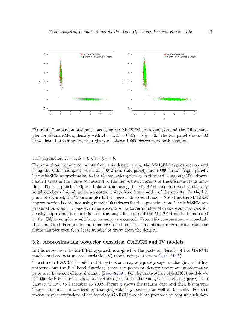
Figure 4: Comparison of simulations using the MitISEM approximation and the Gibbs sam-pler for Gelman-Meng density with A = 1, B = 0, C1 = C2 = 6. The left panel shows 500draws from both samplers, the right panel shows 10000 draws from both samplers.
with parameters A = 1, B = 0, C1 = C2 = 6.
Figure 4 shows simulated points from this density using the MitISEM approximation andusing the Gibbs sampler, based on 500 draws (left panel) and 10000 draws (right panel).The MitISEM approximation to the Gelman-Meng density is obtained using only 1000 draws.Shaded areas in the figure correspond to the high-density regions of the Gelman-Meng func-tion. The left panel of Figure 4 shows that using the MitISEM candidate and a relativelysmall number of simulations, we obtain points from both modes of the density. In the leftpanel of Figure 4, the Gibbs sampler fails to ‘cover’ the second mode. Note that the MitISEMapproximation is obtained using merely 1000 draws for the approximation. The MitISEM ap-proximation would become even more accurate if a larger number of draws would be used fordensity approximation. In this case, the outperformance of the MitISEM method comparedto the Gibbs sampler would be even more pronounced. From this comparison, we concludethat simulated data points and inference based on these simulations are erroneous using theGibbs sampler even for a large number of draws from the density.
3.2. Approximating posterior densities: GARCH and IV models
In this subsection the MitISEM approach is applied to the posterior density of two GARCHmodels and an Instrumental Variable (IV) model using data from Card (1995).
The standard GARCH model and its extensions may adequately capture changing volatilitypatterns, but the likelihood function, hence the posterior density under an uninformativeprior may have non-elliptical shapes (Zivot 2009). For the applications of GARCH models weuse the S&P 500 index percentage returns (100 times the change of the closing price) fromJanuary 2 1998 to December 26 2002. Figure 5 shows the returns data and their histogram.These data are characterized by changing volatility patterns as well as fat tails. For thisreason, several extensions of the standard GARCH models are proposed to capture such data

18 The R package MitISEM
patterns.
0 200 400 600 800 1000 1200
−6
−4
−2
02
46
observations
S&
P 5
00 %
ret
urns
returns
Fre
quen
cy
−6 −4 −2 0 2 4 6
010
2030
4050
Figure 5: Daily log-returns of the S&P 500 index for the period from January 2 1998 toDecember 26 2002.
Approximating posterior densities: A standard GARCH(1,1) model
We first illustrate the use of the MitISEM approach for the Bayesian estimation of the stan-dard GARCH model (Bollerslev 1986) for the S&P 500 data. An extended two-componentGaussian Mixture GARCH (1,1) model (Ausın and Galeano 2007), which possibly leads tomore irregular posterior densities, is considered afterwards.
The standard GARCH(1,1) model for a time series yt (t = 1, 2, . . . , T ) is given by
yt = µ+√ht εt, (13)
ht = ω + α(yt−1 − µ)2 + βht−1, (14)
εt ∼ N(0, 1) i.i.d. (15)
with ht the conditional variance of yt given the information set It−1 = {yt−1, yt−2, yt−3, . . .}.In addition, h0 is treated as a known constant, set as the sample variance of the time seriesyt, which will consist of daily stock index (log) returns in this example.
We restrict ω > 0, α ≥ 0 and β ≥ 0 to ensure positivity of ht. We specify flat priors forthe model parameters. Moreover, we truncate ω and µ such that these have proper (non-informative) priors. For the k = 4 dimensional parameter vector θ = (ω, β, α, µ), we havea uniform prior on [−1, 1] × (0, 1] × [0, 1) × [0, 1) with α + β < 1 which implies covariancestationarity.
The posterior density for the GARCH(1,1) model is implemented as follows:
R> prior.GARCH<-function(omega, beta, alpha, mu, log = TRUE){
+ c1 <- (omega > 0 & omega < 1 & beta >= 0 & alpha >= 0)
+ c2 <- (beta + alpha < 1)
+ c3 <- (mu > -1 & mu < 1)
+ r1 <- c1 & c2 & c3

Nalan Basturk, Lennart Hoogerheide, Anne Opschoor, Herman K. van Dijk 19
+ r2 <- rep.int(-Inf, length(omega))
+ r2[r1==TRUE] <- 0
+ if (!log)
+ r2 <- exp(r2)
+ cbind(r1, r2)
+ }
R> post.GARCH <- function(theta, data, h1, log = TRUE){
+ if (is.vector(theta))
+ theta <- matrix(theta, nrow = 1)
+ omega <- theta[,1]
+ beta <- theta[,2]
+ alpha <- theta[,3]
+ mu <- theta[,4]
+ N <- nrow(theta)
+ pos <- 2:length(data)
+ prior <- prior.GARCH(omega = omega, beta = beta, alpha = alpha,
+ mu = mu)
+ d <- rep.int(-Inf, N)
+ for (i in 1:N){
+ if (prior[i,1] == TRUE){
+ h <- c(h1, omega[i] + alpha[i] * (data[pos-1] - mu[i])^2)
+ for (j in pos)
+ h[j] <- h[j] + beta[i] * h[j-1]
+ tmp <- dnorm(data[pos], mu[i], sqrt(h[pos]), log = TRUE)
+ d[i] <- sum(tmp) + prior[i,2]
+ }
+ }
+ if (!log) d <- exp(d)
+ as.numeric(d)
+ }
The function prior.GARCH is coded outside the kernel function to render the program morereadable and flexible. The function prior.GARCH tests whether the constraints are fulfilled,and outputs a (N × 2) matrix whose first column indicates if the constraints are satisfied,and the second column returns the value of the prior at the corresponding point. Giventhe data vector/matrix and an initial point satisfying the prior parameter constraints, theMitISEM approximation is obtained. Posterior parameter draws can then be obtained usingthe Metropolis-Hastings or rejection sampling algorithm given the candidate constructed byMitISEM, or one can estimate posterior moments using importance sampling. In order to usethe MitISEM candidate for importance sampling or the Metropolis-Hastings algorithm, onecan make use of the function AdMitIS or AdMitMH provided by the R package AdMit, sincethese functions just perform IS or MH using a given candidate that is a mixture of Student-tdistributions. Specifically, the mixture of Student-t distribution obtained from the MitISEMcandidate is used as an input, mit, for functions AdMitIS or AdMitMH for posterior inference.An R code to obtain posterior parameters of the GARCH model is provided below, where weuse the R package tseries, Trapletti and Hornik (2017), to extract S&P 500 data.

20 The R package MitISEM
R> require("tseries")
R> require("AdMit")
R> prices <- as.vector(get.hist.quote("^GSPC", quote = "AdjClose",
+ start = "1998-01-02", end = "2002-12-26"))
R> data <- 100 * (prices[-1] - prices[-length(prices)]) /
+ (prices[-length(prices)])
R> plot(data, xlab = "observation", ylab = "S&P500 % returns")
R> hist(data, xlab = "returns")
R> theta <- c(0.08, 0.86, 0.02, 0.03)
R> names(theta) <- c("omega", "beta", "alpha", "mu")
R> h1 <- var(data);
R> set.seed(1111)
R> app.GARCH <- MitISEM(KERNEL = post.GARCH, mu0 = theta, h1 = h1,
+ data = data, control = list(trace = TRUE))
1 1 BFGS 0.76 1.1352420 1.135242e-04
2 1 IS-EM 28.70 0.7567956 7.567956e-05
3 2 IS-EM 57.91 0.4105256 4.105256e-05
4 3 IS-EM 56.76 0.3864224 3.864224e-05
R> IS.GARCH <- AdMitIS(N = 10e4, KERNEL = post.GARCH,
+ mit = app.GARCH$mit, data = data, h1 = h1)
R> print(IS.GARCH)
$ghat
[1] 0.08884915 0.84851733 0.10637618 0.03354568
$NSE
[1] 1.158643e-04 1.133241e-04 7.695703e-05 1.187978e-04
$RNE
[1] 0.6974687 0.7058110 0.7292880 0.8363404
The summary output of the function MitISEM is a data frame containing information onthe adaptive fitting procedure: H is the number of Student-t components; METHOD indicateswhether the IS-weighted EM algorithm has been used to optimize the candidate (where theBFGS method has been used to compute the mode of the target density); TIME gives thecomputing time required for this optimization; CV gives the coefficient of variation of theimportance sampling weights; std.dev. gives the standard deviation of the IS weights.The output of the function AdMitIS is a list. The first component is ghat, the importance
sampling estimator G =
∑N
i=1W iG(θi)∑N
i=1W i
of the property of interest E[G(θ)], which is in our case
the posterior mean of the parameters. The second component is NSE, a vector containing thenumerical standard errors (i.e., the standard deviation of the estimates that can be expectedif the simulations were to be repeated) of the components of ghat. The third component isRNE, a vector containing the relative numerical efficiencies of the components of ghat (i.e.,the ratio between the estimated variance of a hypothetical estimator based on direct samplingand the importance sampling estimator’s estimated variance with the same number of draws).RNE is an indicator of the efficiency of the chosen importance density; if target and importance
Nalan Basturk, Lennart Hoogerheide, Anne Opschoor, Herman K. van Dijk 21
densities coincide, RNE equals one, whereas a very poor importance density will have a RNE
close to zero. Both NSE and RNE are estimated by the method given in Geweke (1989).For estimating E[G(θ)] the N candidate draws are approximately as ‘valuable’ as RNE × Nindependent draws from the target would be.
The MitISEM approximation of the posterior density consists of 3 Student-t components. Thelow CoV values and the high RNE values show that the MitISEM candidate approximatesthe posterior density accurately.
Approximating posterior densities: A mixture GARCH(1,1) model
In this subsection the MitISEM approach is applied to the non-elliptical posterior densityin the two-component Gaussian Mixture GARCH (1,1) model of Ausın and Galeano (2007).For the Bayesian estimation of this model, Ausın and Galeano (2007) propose a griddy Gibbssampler (Ritter and Tanner 1992), since the recursive structure of the likelihood in GARCH-type models implies that a regular Gibbs sampling approach is not feasible.
The griddy Gibbs sampler is known to be very slow. As an alternative we use importancesampling with a candidate density resulting from the MitISEM algorithm, and compare theperformance of the MitISEM candidate density with the naive Student-t candidate densityand a candidate obtained from the AdMit method.
The two-component Gaussian mixture GARCH(1,1) model for the returns yt (t = 1, 2, . . . , T )is given by
yt = µ+√ht εt, (16)
ht = ω + α(yt−1 − µ)2 + βht−1, (17)
εt ∼{N(0, σ2) with probability ρ,N(0, σ2/λ) with probability 1− ρ,
(18)
with ht the conditional variance of yt given the information set It−1 = {yt−1, yt−2, yt−3, . . .}.In addition, 0 < λ < 1, and σ2 ≡ 1/(ρ + (1 − ρ)/λ) so that var(εt) = 1; h0 is treated as aknown constant, set as the sample variance of the return series. We restrict ω > 0, α ≥ 0 andβ ≥ 0 to ensure positivity of ht. We follow Ausın and Galeano (2007) by imposing the priorrestriction 0.5 < ρ < 1, so that it is ensured that the state with smaller variance has largerprobability than the state with larger variance. The mixture distribution in (18) has fattertails than a Gaussian distribution. We follow Ausın and Galeano (2007) also in specifying flatpriors for the model parameters. Moreover, we truncate ω and µ such that these have proper(non-informative) priors. For the k = 6 dimensional parameter vector θ = (ω, λ, β, α, ρ, µ),we have a uniform prior on (0, 1] × (0, 1) × [0, 1) × [0, 1) × (0.5, 1] × [−1, 1] with α + β < 1which implies covariance stationarity.
The posterior density for the Gaussian mixture GARCH(1,1) model is implemented as follows:
R> prior.mGARCH<-function(omega, lambda, beta, alpha, rho, mu,
+ log = TRUE){
+ c1 <- (omega > 0 & omega < 1 & beta >= 0 & alpha >= 0)
+ c2 <- (beta + alpha< 1)
+ c3 <- (lambda >= 0 & lambda <= 1)
+ c4 <- (rho>0.5 & rho<1)

22 The R package MitISEM
+ c5 <- (mu>-1 & mu<1)
+ r1 <- c1 & c2 & c3 & c4 & c5
+ r2 <- rep.int(-Inf, length(omega))
+ tmp <- log(2)
+ r2[r1==TRUE] <- tmp
+ if (!log)
+ r2 <- exp(r2)
+ cbind(r1, r2)
+ }
R> post.mGARCH <- function(theta, data, h1, log = TRUE){
+ if (is.vector(theta))
+ theta <- matrix(theta, nrow = 1)
+ omega <- theta[,1]
+ lambda <- theta[,2]
+ beta <- theta[,3]
+ alpha <- theta[,4]
+ rho <- theta[,5]
+ mu <- theta[,6]
+ N <- nrow(theta)
+ pos <- 2:length(data)
+ prior <- prior.mGARCH(omega = omega, lambda = lambda,
+ beta = beta, alpha = alpha, rho = rho, mu = mu)
+ d <- rep.int(-Inf,N)
+ for (i in 1:N){
+ if (prior[i,1] == TRUE){
+ h <- c(h1, omega[i] + alpha[i] * (data[pos-1]-mu[i])^2)
+ for (j in pos){
+ h[j] <- h[j] + beta[i] * h[j-1]
+ }
+ sigma <- 1 / (rho[i] + ((1-rho[i]) / lambda[i]))
+ tmp1 <- dnorm(data[pos], mu[i], sqrt(h[pos] * sigma),
+ log = TRUE)
+ tmp2 <- dnorm(data[pos], mu[i], sqrt(h[pos] * sigma /
+ lambda[i]), log = TRUE)
+ tmp <- log(rho[i] * exp(tmp1) + (1 - rho[i]) * exp(tmp2))
+ d[i] <- sum(tmp) + prior[i,2]
+ }
+ }
+ if (!log)
+ d <- exp(d)
+ as.numeric(d)
+ }
Given the data vector/matrix data the MitISEM approximation is calculated starting froman initial point satisfying the prior parameter constraints. Posterior parameter draws (orappropriately weighted candidate draws) are then obtained using the Metropolis-Hastingsalgorithm (or importance sampling) given the candidate constructed by MitISEM.

Nalan Basturk, Lennart Hoogerheide, Anne Opschoor, Herman K. van Dijk 23
Given the MitISEM candidate, one can again obtain importance sampling results using theAdMitIS function provided by the R package AdMit, where the MitISEM candidate is usedas an input to AdMitIS
R> require("tseries")
R> require("AdMit")
R> prices <- as.vector(get.hist.quote("^GSPC", quote = "AdjClose",
+ start = "1998-01-02", end = "2002-12-26"))
R> data <- 100 * (prices[-1] - prices[-length(prices)])/
+ (prices[-length(prices)])
R> mu0 <- c(0.08, 0.37, 0.86, 0.03, 0.82, 0.03)
R> names(mu0) <- c("omega", "lambda", "beta", "alpha", "rho", "mu")
R> h1 = var(data);
R> set.seed(1234)
R> app.mGARCH <- MitISEM(KERNEL = post.mGARCH, mu0 = mu0, h1 = h1,
+ data = data)
R> app.mGARCH$summary
H METHOD TIME CV IS weights std.dev.
1 1 BFGS 2.03 2.1170292 2.117029e-04
2 1 IS-EM 25.97 1.5332795 1.533280e-04
3 2 IS-EM 56.01 1.0081923 1.008192e-04
4 3 IS-EM 60.32 0.8610536 8.610536e-05
5 4 IS-EM 58.75 0.7905704 7.905704e-05
R> IS.mGARCH <- AdMitIS(N = 10e4, KERNEL = post.mGARCH,
+ mit = app.mGARCH$mit, data = data, h1 = h1)
R> print(IS.mGARCH,2)
$ghat
[1] 0.079 0.369 0.862 0.099 0.788 0.029
$NSE
[1] 1.4e-04 3.7e-04 1.3e-04 9.2e-05 5.8e-04 1.4e-04
$RNE
[1] 0.47 0.51 0.50 0.51 0.46 0.61
MitISEM method and the AdMit method (for which no output is shown above, since ourmain focus is on the novel MitISEM package) yield an approximation that is a mixture of 7and 4 Student-t components. The conditional posterior density kernel of parameters (ρ, λ)given that the other four parameters are equal to their (estimated) posterior means and theapproximations by three methods are shown in Figure 6. The MitISEM density is clearlythe best approximation of the posterior. Table 1 and Table 2 show that for this example,both ‘naive’ and MitISEM candidates outperform the AdMit approximation in terms of theimportance weights’ CoV, and in terms of the NSEs of the estimated posterior means. Thereare two reasons for the better performance of the ‘naive’ candidate compared with the AdMitcandidate. First, the IS-weighted EM algorithm implies that the ‘naive’ candidate’s singleStudent-t density is specified in an optimal way. Second, the novel robustification introduced

24 The R package MitISEM
in this paper, discarding candidate draws outside the ‘allowed range’ from the number ofcandidate draws during the construction of a new candidate, ensures that enough relevant,‘allowed’ candidate draws are obtained for the construction of the ‘naive’ candidate. In par-ticular for target densities with several parameter restrictions, such as the posterior in themixture GARCH model, this robustification is important. Further, the additional Student-tcomponents of the MitISEM candidate imply that it has a higher accuracy than the ‘naive’candidate. First, if we require simulation results with a certain very high precision, then Mi-tISEM would obviously require much fewer draws than the ‘naive’ and AdMit approximations,so that the total computing time (for both the construction and the subsequent use of thecandidate density) would be shorter for MitISEM. Second, the higher quality of the MitISEMapproximation of the target density compared to ‘naive’ and AdMit approximations impliesthat there is less risk that a relevant part of the target density is ‘missed’, for example in caseof a multi-modal target density, which would possibly cause substantially biased results forthe other methods.
Algorithm # t Components Time (seconds) CoV
AdMit 4 144.30 2.61Naive 1 19.40 2.47MitISEM 7 358.57 0.72
Table 1: Summary of naive, AdMit and MitISEM candidates for the mixture GARCH(1,1)model for S&P 500 data. The table reports the algorithm for obtaining the candidate distri-bution, the number of Student-t components (# t), time (in seconds) and CoV (coefficient ofvariation of the IS weights) for all compared algorithms. Candidates are constructed using104 draws.
Posterior mean NSE ×100
AdMit Naive MitISEM AdMit Naive MitISEM
ω 0.08 0.08 0.08 0.09 0.06 0.07λ 0.38 0.37 0.37 0.25 0.24 0.12β 0.86 0.86 0.86 0.09 0.06 0.06α 0.10 0.10 0.10 0.06 0.04 0.03ρ 0.78 0.78 0.78 0.43 0.32 0.21µ 0.03 0.03 0.03 0.10 0.07 0.04
Table 2: Estimated posterior means of parameters in mixture GARCH(1,1) model and Nu-merical Standard Errors (NSE) of the IS estimates using the naive, AdMit and MitISEMcandidates for the S&P 500 data. Candidate approximations and posterior results are basedon 104 and 103 draws, respectively.
Approximating posterior densities: An IV model
In this subsection we apply the MitISEM algorithm to an Instrumental Variables (IV) regres-sion model. We first make use of a set of simulated data and report the accuracy of posteriorinference from the Metropolis-Hastings and importance sampling algorithms based on a Mi-

Nalan Basturk, Lennart Hoogerheide, Anne Opschoor, Herman K. van Dijk 25
0.5 0.6 0.7 0.8 0.9
0.1
0.2
0.3
0.4
0.5
0.6
0.7
0.8
ρ
λ
0.5 0.6 0.7 0.8 0.9
0.1
0.2
0.3
0.4
0.5
0.6
0.7
0.8
ρ
λ
conditional posterior naive candidate
0.5 0.6 0.7 0.8 0.9
0.1
0.2
0.3
0.4
0.5
0.6
0.7
0.8
ρ
λ
0.5 0.6 0.7 0.8 0.9
0.1
0.2
0.3
0.4
0.5
0.6
0.7
0.8
ρ
λ
AdMit candidate MitISEM candidate4 components 4 components
Figure 6: Conditional posterior density kernel of (ρ, λ) given posterior means of the otherparameters (ω, β, α, µ) in the mixture GARCH(1,1) model together with the naive, AdMitand MitISEM approximations.
tISEM approximation to the posterior density and compare the results with those obtainedusing the griddy Gibbs sampler of Ritter and Tanner (1992). The griddy Gibbs algorithmthat we specify uses the inverse CDF technique to obtain posterior draws for each parameter.3
Second, we use empirical data from Card (1995) and apply the MitISEM algorithm to an IVmodel that describes the effect of years of education on earned income.
The IV model with one explanatory endogenous variable and p instruments is defined by(Bowden and Turkington 1990):
y = xβ + ε, (19)
x = zΠ + v, (20)
3A replication routine for this simulation study is provided in replication scripts of the paper.
26 The R package MitISEM
where the scalar β and the p × 1 vector Π are model parameters, y is the N × 1 vector ofobservations on the dependent variable income, x is the N × 1 vector of observations on theendogenous explanatory variable, education, z is the N × p matrix of observations on theinstruments. All variables are demeaned, i.e., both model equations do not include a constantterm. The disturbances are assumed to come from a normal distribution: (ε>, v>)> ∼
NID(0,Σ⊗ I), where Σ =
(σ211 ρσ11σ22
ρσ11σ22 σ222
)is a positive definite and symmetric 2× 2
matrix, I denotes the N ×N identity matrix and ⊗ denotes the Kronecker product operator.
‘Endogeneity’ of the variable x arises from possible correlation between the disturbances,given as ρ ≡ cor (εi, vi) for i = 1, . . . , N . The effect of latent abilities (leading to both ahigher education and a higher income given a certain education level) may cause a positivecorrelation ρ, whereas measurement errors in observed education may cause a negative ρ. Wenote that in case the covariance matrix Σ is diagonal, the IV model simplifies to a simpleregression model, with elliptical posterior densities (Zellner 1971). Therefore the instrumentsare only necessary if the correlation between the disturbances is different from zero.
Under conventional flat priors, it can be shown that the posterior density for the parametersfor the IV model is non-standard (Dreze 1976, 1977; Kleibergen and Van Dijk 1998). Foran exactly identified model with a single instrument, the posterior density resulting fromthis model is improper. For more details on the derivation we refer to Zellner et al. (2014).We specify a Jeffreys prior which leads to a proper posterior density, see e.g., Hoogerheide,Kleibergen, and Van Dijk (2007a) for the derivation. The posterior density of the model inEquations 19-20 under the Jeffreys prior can be implemented as follows:
R> Jeff.prior<-function(beta, Pi, Sigma11, rho, Sigma22){
+ c1 <- (Sigma11 > 0)
+ c2 <- (Sigma22 > 0)
+ c3 <- (rho > -1)
+ c4 <- (rho < 1)
+ r1 <- c1 & c2 & c3 & c4
+ r2 <- rep.int(-Inf, length(Sigma11))
+ r2[r1==TRUE] <- log(abs(Pi[r1==TRUE])) - 2 * log(Sigma11[r1==TRUE]
+ * Sigma22[r1==TRUE] * (1- rho[r1==TRUE]^2))
+ return(cbind(r1, r2))
+ }
R> post.IV<-function(theta, data, log = TRUE){
+ if(is.vector(theta))
+ theta = matrix(theta, nrow = 1)
+ y <- data[,1]
+ x <- data[,2]
+ z <- data[,3]
+ if (is.vector(theta))
+ theta <- matrix(theta, nrow = 1)
+ logprior <- Jeff.prior(theta[,1], theta[,2], theta[,3], theta[,4],
+ theta[,5])
+ rcov <- logprior[,1] == TRUE
+ fn_aux <- function(theta_aug,y,x,z){

Nalan Basturk, Lennart Hoogerheide, Anne Opschoor, Herman K. van Dijk 27
+ tmp <- matrix(c(theta_aug[3], theta_aug[4], theta_aug[4],
+ theta_aug[5]), 2, 2)
+ detfac <- log(det(tmp))
+ beta <- theta_aug[1]
+ Pi <- theta_aug[2]
+ res <- cbind(y - x * beta, x - z * Pi)
+ SigmaInv <- solve(tmp)
+ S <- SigmaInv %*% crossprod(res)
+ expfac <- -0.5*sum(diag(S))
+ (c(detfac,expfac))
+ }
+ theta_aug = theta[rcov,]
+ if(is.vector(theta_aug))
+ theta_aug = matrix(theta_aug, nrow = 1)
+ Sigma12 <- theta[rcov,4] * sqrt(theta[rcov,3] * theta[rcov,5])
+ theta_aug[,4] = Sigma12
+ T <- length(y)
+ d <- rep.int(-Inf, nrow(theta))
+ if(any(rcov)){
+ tmp_1 = t(apply(theta_aug, 1, FUN = fn_aux, y = y, x = x, z = z))
+ d[rcov] = - (T/2) * tmp_1[,1] + tmp_1[,2] + logprior[rcov,2]
+ }
+ if (!log)
+ d <- exp(d)
+ as.numeric(d)
+ }
As mentioned, we first apply the MitISEM method to artificial data for the case of an IVmodel. We simulate 300 observations from the IV model in Equations 19 and 20, with ‘true’parameter values (β, π, σ211, ρ, σ
222) = (0.73, 0.06, 0.21,−0.43, 0.17). These values correspond
to the posterior means of the parameters in the real data application, using Card (1995).Posterior results from MH and IS methods using the MitISEM approximation to the posteriordensity are obtained using the functions AdMitMH and AdMitIS in the R package AdMit.Specifically, the MitISEM candidate is used as an input to AdMitMH and AdMitIS functions.These two functions perform sampling from the MitISEM candidate and posterior inferenceusing the MitISEM candidate. The MitISEM approximation to the posterior density is basedon 10000 draws, leading to a 3-component mixture of Student-t densities, i.e., the posteriordensity is highly non-elliptical. For the Metropolis-Hastings algorithm we use 10000 burn-indraws and 10000 posterior draws. Importance sampling results are based on 10000 draws. Thealternative method, the griddy Gibbs sampler, is based on 10000 posterior draws, and 10000burn-in draws. For each parameter draw using the griddy Gibbs sampler, 200 equi-distantgrid points are taken on the parameter space β ∈ [−2, 2], π ∈ [−2, 2], (σ211, σ
222) ∈ (0, 2]2 and
ρ ∈ (−1, 1).
Estimated posterior means and standard deviations for parameters using the three samplingalgorithms are shown in Table 3.4 The griddy Gibbs sampling results are very different
4We emphasize that Bayesian posterior analysis, using a Jeffreys prior, does not necessarily yield posterior

28 The R package MitISEM
from the MH and IS results using the MitISEM candidate. In particular, posterior drawsof the correlation coefficient ρ are concentrated around 0.06 with a relatively small standarddeviation compared to results from MH and IS. This indicates that the griddy Gibbs samplerfails to cover the whole domain of the posterior density and it is seen that the MitISEMapproximation substantially improves the simulation inference for this example. We alsocomputed two convergence test results for griddy Gibbs draws as well as for MH draws (thatare based on a MitISEM approximation to the posterior). Results are obtained using theR package MCMCpack, Martin, Quinn, and Park (2011, 2017). P-values are based on aconvergence criterion presented in Geweke (1992), where the null hypothesis is the equalityof posterior means from the first and last parts of the Markov Chain. At the 5% level, thenull hypothesis is not rejected for griddy Gibbs draws as well as for the MH results althoughthe posterior mean estimates are numerically different. We additionally report results forthe Heidelberger and Welch (1981) test where the null hypothesis is that the samples ofposterior draws come from a stationary distribution. According to this test, β and ρ drawsfrom the griddy Gibbs sampler do not come from a stationary distribution while all drawsfrom MH ‘pass’ the test. These test results show that these tests are rather sensitive to theexact specification of the test and we recommend the use of multiple tests for convergenceassessment.
The relatively poor performance of the griddy Gibbs sampler is clearly shown in Figure 7 and8, where we present draws from (β, π, ρ) and the traceplot of all parameters from the MHalgorithm and the griddy Gibbs sampler. The left panel of Figure 7 shows that the griddyGibbs sampler leads to many draws of (β, π) that are far from the central part of the posteriorwhile draws from the MH algorithm using the MitISEM approximation are relatively moreconcentrated in that center. Similarly, on the right panel of Figure 7, relatively more (β, ρ)draws from the griddy Gibbs sampler are far from the important region of the posterior andlie at the bottom right area of the figure compared to MH draws. A reason for this poorperformance is the much higher serial correlation between griddy Gibbs draws compared toMH draws. This is shown in Figure 8. Griddy Gibbs draws are strongly serially correlated,particularly for parameters (β, ρ), while MH draws using the MitISEM candidate have very fewconsecutive draws with same parameter values. We conclude that the griddy Gibbs sampleris much less accurate given the same number of draws compared to IS and MH algorithmsusing the MitISEM approximation as the candidate density.5
We next apply the MitISEM algorithm to approximate the posterior density of the IV modelin Equations 19 and 20 for the Card (1995) data on income and education, and compare theresults with those obtained from the griddy Gibbs sampler. In these data, income levels aremeasured by hourly wage (in natural logarithms), education level is 1 if the individual attendedcollege and 0 otherwise. College proximity, which takes the value 1 if there is a nearby collegeand 0 otherwise, is the proposed instrument for the education level of individuals. The datafurther consist of other covariates such as gender, experience and area of residence for 1030men in 1976.6 For the analysis of the IV model, we first demean the income, education and
means that are equal to the so-called ‘true’ parameter values. The difference may due to a flat or skew posteriorand/or a relatively small sample.
5When the number of draws is increased to 10000 burn-in and 20000 posterior draws, the slight difference inMH and IS parameter estimates disappear, while posterior results for the griddy Gibbs sampler remain similarto those in Table 3.
6Data can be obtained from davidcard.berkeley.edu/data_sets/proximity.zip. The data includes sev-eral additional covariates compared to the standard model outlined in this section. Relevant variables need

Nalan Basturk, Lennart Hoogerheide, Anne Opschoor, Herman K. van Dijk 29
β π σ211 ρ σ222 Time
True values 0.73 0.06 0.21 -0.43 0.17
Posterior means and standard deviations
Griddy Gibbs Mean 0.13 0.05 0.15 0.10 0.16 2728Std. dev. 0.09 0.02 0.01 0.10 0.01
MH Mean 0.76 0.06 0.22 -0.44 0.17 64Std. dev. 0.33 0.02 0.07 0.22 0.01
IS Mean 0.76 0.06 0.21 -0.44 0.16 62Std. dev. 0.30 0.02 0.06 0.20 0.01
Table 3: Estimated posterior means and standard deviations of parameters for simulated IVdata based on griddy Gibbs sampler and MH and IS algorithms using MitISEM approxima-tion. MitISEM candidate is based on 10000 draws. MH and griddy Gibbs results are basedon 10000 posterior and 10000 burn-in draws. IS results are based on 10000 draws. For thegriddy Gibbs sampler we use 200 grid points for each parameter. The last column of the tablereports the elapsed time for each posterior sampler in minutes. For IS and MH algorithmswe report total time, including the time required to construct the MitISEM candidate.
-0.05 0.00 0.05 0.10
-0.5
0.0
0.5
1.0
1.5
p
b
griddy GibbsMH
-0.5 0.0 0.5
-0.5
0.0
0.5
1.0
1.5
r
b
griddy GibbsMH
Figure 7: Parameter (β, π) and (β, ρ) draws for simulated IV data based on the griddy Gibbssampler and the MH algorithm using MitISEM approximation. Horizontal and vertical linesare the true parameter values. Posterior results are obtained as in Table 3.

30 The R package MitISEM
1000 2000 3000 4000 5000
-0.5
0.0
0.5
1.0
1.5
2.0
griddy Gibbs posterior draw
b p s12 r s2
2
1000 2000 3000 4000 5000
-0.5
0.0
0.5
1.0
1.5
2.0
MH posterior draw
b p s12 r s2
2
Figure 8: Posterior draws of all parameters for simulated IV data based on the griddy Gibbssampler and the MH algorithm using MitISEM approximation. Posterior results are obtainedas in Table 3.
college proximity data, and transform these into residuals after regression on the exogenouscovariates in the dataset, which is equivalent to integrating out the corresponding coefficientsunder a flat prior.
Similar to the simulation study, the griddy Gibbs sampling results are different from theMetropolis-Hastings and importance sampling results using the MitISEM candidate, as seenin Table 4. Here, posterior draws from the correlation coefficient ρ are concentrated around0.12 with again a relatively small standard deviation. This small standard deviation confirmsthat the griddy Gibbs sampler fails to cover the whole domain of the posterior density andthat the MitISEM approximation substantially improves the simulation inference for thesedata.
3.3. Approximating model probabilities using the concept of predictivelikelihoods
In this subsection we show how the candidate density obtained by the MitISEM method canbe used to accurately calculate a model’s predictive likelihood. The calculation of modelprobabilities can be based on the models’ marginal likelihoods or the predictive likelihoods,where the former are problematic under non-informative priors on parameters that only occurin one of the models, in the sense that the ‘smaller’ model may be favored even if the ‘larger’model is the true Data Generating Process (DGP) (Bartlett 1957). The MitISEM packageprovides functions to calculate the marginal or predictive likelihood of a model given itsposterior density kernel and a candidate density obtained by the MitISEM method. Thereason is that the computation of marginal or predictive likelihoods is an important ingredientof many Bayesian analyses.
The predictive likelihood of a model M1 is obtained by splitting the data y = (y1, . . . yT ) intoy∗ = (y1, . . . ym) and y = (ym+1, . . . yT ) (Gelfand and Dey 1994; Eklund and Karlsson 2007):
p(y|y∗,M1) =
∫p(y|θ1, y∗,M1)p(θ1|y∗,M1)dθ1, (21)
to be extracted using the authors’ codebook in the website. The R code to prepare Card (1995) data for theexample IV model is supplied in replication scripts.

Nalan Basturk, Lennart Hoogerheide, Anne Opschoor, Herman K. van Dijk 31
β π σ211 ρ σ222 Time
Griddy Gibbs Mean 0.11 0.05 0.15 0.12 0.16 23.7Std. dev. 0.09 0.02 0.01 0.10 0.01
MH Mean 0.73 0.07 0.21 -0.43 0.17 1.1
Std. dev. 0.28 0.02 0.05 0.20 0.00(∗)
IS Mean 0.73 0.06 0.21 -0.43 0.17 1.1
Std. dev. 0.28 0.02 0.05 0.20 0.00(∗)
Table 4: Estimated posterior means and standard deviations of parameters for the IV modelfor Card (1995) data obtained using the griddy Gibbs sampler, Metropolis-Hastings algorithmbased on the MitISEM candidate and importance sampling based on the MitISEM candidate.MitISEM candidate is based on 104 draws. MH and griddy Gibbs results are based on 5000posterior and 5000 burn-in draws. IS results are based on 10000 draws. For the griddy Gibbssampler we use 200 grid points for each parameter. The last column of the table reports theelapsed time for each posterior sampler in minutes. For IS and MH algorithms we report totaltime, including the time required to construct the MitISEM candidate. For values indicatedby (∗), the standard deviation is 0.0044 at the 4-digit level.
which is the marginal likelihood if we consider y as ‘the data’ and p(θ1|y∗,M1), the exactposterior density, i.e., density including the normalizing constant, and the posterior kernel,after observing y∗, as the prior. Using Bayes’ rule for this exact posterior density p(θ1|y∗,M1)and substituting into Equation 21 yields
p(y|y∗,M1) =
∫p(y|θ1,M1)p(θ1|M1)dθ1∫p(y∗|θ1,M1)p(θ1|M1)dθ1
, (22)
where p(θ1|M1) is the prior on model parameters θ1 for model M1. Hence this predictive like-lihood is the ratio of the marginal likelihood for all observations over the marginal likelihoodfor the first part of the data. The integral in Equation 22 can be evaluated by numerical in-tegration using θ1 draws obtained from the Metropolis-Hastings algorithm in package AdMitusing the MitISEM candidate density.
Model probability for M1 is then calculated using the posterior density in Equation 22
p(M1|y) = p(M1|y, y∗) =p(M1|y∗)p(y|y∗,M1)
p(y|y∗)∝ p(M1|y∗)p(y|y∗,M1), (23)
where (p(y|y∗))−1, which is independent of the model M1, is the normalizing constant andp(M1|y∗) is the prior model probability conditional on prior data points y∗. In practice, thisprior model probability is often defined independent of prior data points and ensures equalprior model weights.
Approximating model probabilities using predictive likelihood: A mixture GARCH(1,1)model
As a first illustration, we apply the model in (16)–(18) to S&P 500 data and perform thesimulation-based computation of the predictive likelihoods. We also compare the performanceof the MitISEM candidate with a ‘naive’ candidate. The first half of the observations are

32 The R package MitISEM
regarded as the ‘training sample’ y∗ = (y1, . . . ym). Predictive likelihood calculation using theMitISEM approximation is implemented as:
R> library("MitISEM")
R> library("tseries")
R> source("PostmGARCH.R")
R> prices <-as.vector(get.hist.quote("^GSPC", quote = "AdjClose",
+ start = "1998-01-02", end = "2002-12-26"))
R> data <- 100 * (prices[-1] - prices[-length(prices)]) /
+ (prices[-length(prices)])
R> data.ss <- data[1:626]
R> h1 <- var(data)
R> mu0 <- c(0.08, 0.37, 0.86, 0.03, 0.82, 0.03)
R> names(mu0) <- c("omega", "lambda", "beta", "alpha", "p", "mu")
R> set.seed(1234)
R> mit.ss <- MitISEM(KERNEL = post.mGARCH, mu0 = mu0, data = data.ss,
+ h1 = h1, control=list(trace=TRUE))$mit
R> mit.fs <- MitISEM(KERNEL = post.mGARCH, mu0 = mu0, data = data,
+ h1 = h1, control=list(trace=TRUE))$mit
R> PL.mGARCH <- PredLik(N,mit.fs, mit.ss, post.mGARCH, data, data.ss, h1=h1)
where the posterior density function for the mixture of GARCH(1,1) is defined as in Sec-tion 3.2.2, y.ss is the training sample of 626 observations for predictive likelihood calcula-tions, the initial variance h1 of the GARCH model is defined as the sample variance of thedata, initial parameters are defined as mu0 and predictive likelihood calculation is based on N
draws.
In order to calculate the accuracy of the estimates, we replicate the predictive likelihoodcalculation 50 times. Table 5 shows simulation results where the average predictive likelihoodsand Numerical Standard Errors are calculated from 50 replications. The candidates for allcases are calculated using 104 draws, and the estimated predictive likelihood values are basedon 103 draws, where the latter was done to decrease the computing time of the 50 repetitions.
# t components Predictive likelihoodTraining sample Full sample Mean NSE
4 3 1.68 ×10−470 1.28 ×10−472
Table 5: Approximation and predictive likelihood for the mixture of GARCH model. Candi-date approximations and posterior results are based on 104 and 103 draws, respectively. Meanand Numerical Standard Error (NSE) for each estimate are based on 50 replications.
The MitISEM candidate consists of four and three mixture components for the training sampleand the full sample, respectively, indicating highly non-elliptical posterior shapes for bothdatasets. Despite these irregularities in the posterior densities, the small NSE reported inTable 5 shows that, even with the relatively small number of posterior draws, calculatedpredictive likelihoods for this model are quite accurate given the MitISEM approximation tothe posterior density.

Nalan Basturk, Lennart Hoogerheide, Anne Opschoor, Herman K. van Dijk 33
Computing a sequence of predictive likelihoods using sequential MitISEM
We next apply the sequential MitISEM algorithm to the two-component mixture GARCHmodel with the S&P 500 data. Sequential MitISEM is used to efficiently construct a series ofcandidates that approximate posteriors for increasing data sets, where the candidate can beused for estimation of posterior moments, marginal likelihoods or predictive likelihoods. Inthis example we consider the latter. We use the first half of the observations as the trainingsample y∗ (for the marginal likelihood in the denominator of the predictive likelihood inEquation 22). At each time t = 1204, . . . , 1252, the predictive likelihood is computed whilethe training sample y∗ is kept fixed. Such a sequence of updated predictive likelihoods couldbe used in an application of Bayesian model averaging (BMA), combining forecasts fromseveral models at each time t = 1204, . . . , 1252 by weighting these with the estimated modelprobabilities. Once the posterior kernel is specified, the sequential MitISEM approximationscan be obtained as follows:
R> require("tseries")
R> require("AdMit")
R> prices <- as.vector(get.hist.quote("^GSPC", quote = "AdjClose",
+ start = "1998-01-02", end = "2002-12-26"))
R> data <- 100 * (prices[-1] - prices[-length(prices)]) /
+ (prices[-length(prices)])
R> mu0 <- c(0.08, 0.37, 0.86, 0.03, 0.82, 0.03)
R> names(mu0) <- c("omega", "lambda", "beta", "alpha", "rho", "mu")
R> h1 = var(data)
R> data.ss <- data[1:floor(length(data) / 2)]
R> MitISEMapp.subsample <- MitISEM(KERNEL = post.mGARCH, mu0 = mu0, h1 = h1,
+ data = data.ss)
R> control.seq <- list(T0 = 1203, tau = 1:20)
R> app.mGARCH.SeqMitISEM <- SeqMitISEM(data, KERNEL = post.mGARCH, mu0 = mu0,
+ control.seq = control.seq, h1 = h1)
Table 6 presents the number of mixture components, CoV values and estimated predictivelikelihoods for each sequential algorithm, and provides more details about the results of thesequential MitISEM algorithm. Note that for the calculation of predictive likelihoods inincreased data samples, an ‘ad hoc’ MitISEM procedure would be applied 20 times, whilethe sequential MitISEM ‘adopts’ the candidate density only once for sample size 1208 and‘extends’ the candidate density only once for sample size 1209. In the remaining time periods,the candidate is simply ‘reused’, with minimal computational time. Table 6 shows thatthe MitISEM approximation using a subsample of the data is ‘reused’ 18 times, indicationapproximately 18 times speed gains compared to the standard MitISEM approximation foreach sample. Similarly, one MitISEM candidate is only ‘adjusted’, again providing speedgains compared to employing the whole MitISEM algorithm for each subsample. Note thatthe CoV values remain low, so that the huge gains in computing time do not lead to a badquality of the candidate distribution.
Approximating model probabilities using predictive likelihood: An IV model
As a third application of predictive likelihood approximations using the MitISEM algorithm,we consider the IV model in Equation 19 and Equation 20 with the Jeffreys prior for the Card

34 The R package MitISEM
#Observations #t CoV Predictive likelihood
1204 3 0.98 3.76×10−435
1205 3 1.01 0.64×10−435
1206 3 0.95 0.83×10−436
1207 3 1.04 1.35×10−437
1208 6 0.99 2.36×10−438
1209 6∗ 0.72 3.57×10−439
1210 6 0.72 0.50×10−439
1211 6 0.72 1.04×10−440
1212 6 0.73 2.09×10−441
1213 6 0.85 3.93×10−442
1214 6 0.76 0.97×10−442
1215 6 0.76 1.27×10−443
1216 6 0.75 2.97×10−444
1217 6 0.81 0.75×10−444
1218 6 0.82 1.81×10−445
1219 6 0.72 1.17×10−446
1220 6 0.77 2.59×10−447
1221 6 0.73 2.22×10−448
1222 6 0.74 0.52×10−448
1223 6 0.74 1.43×10−449
Sequential MitISEM steps
# reused 18# adapted 1# adapted and extended 1
Table 6: Predictive Likelihoods for the mixture GARCH model using sequential MitISEM.Candidate approximations and posterior results are based on 104 and 103 draws, respectively.#t denotes the number of Student-t components in MitISEM approximation. (∗) indicatesthat the candidate density from the previous approximation is adapted.
data on income and education described in Section 3.1. We define two models, one treatingeducation as an endogenous explanatory variable (i.e., the IV model in Equation 19 andEquation 20, and the second model treating education as an exogenous explanatory variable(i.e., the simple linear regression model). The linear regression model is a nested modelcompared to the IV model in Equation 19 and Equation 20 with the parameter restrictionρ = 0 and posterior inference for the effect of education on income, β, in this case is basedonly on Equation 19. For a comparison of these two models under uninformative priors, weuse the predictive likelihoods. The predictive probability of the null model (which assumesexogeneity) can be calculated using the Savage-Dickey Density Ratio (SDDR). Dickey (1971)shows that the Bayes factor can be calculated using a single model if the null model is arestricted version of the alternative model and the prior densities satisfy the condition thatthe prior for the restricted model equals the corresponding conditional prior (conditionalupon satisfying the restriction) in the unrestricted model. Under that condition the model
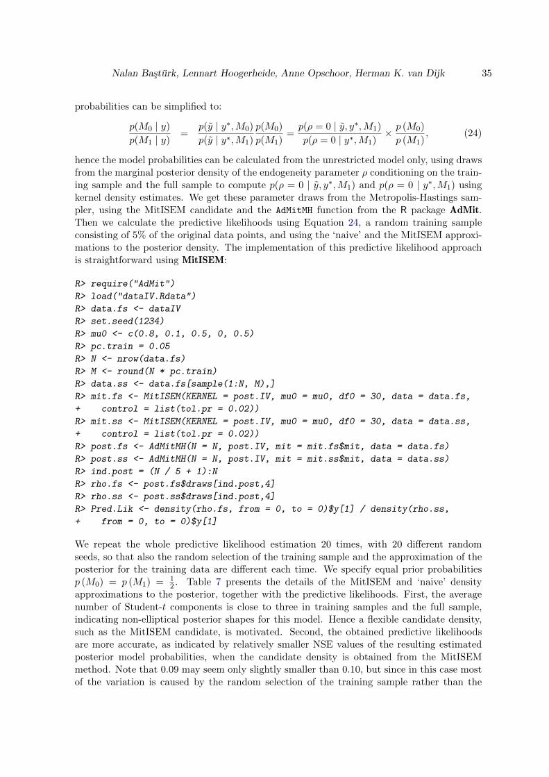
Nalan Basturk, Lennart Hoogerheide, Anne Opschoor, Herman K. van Dijk 35
probabilities can be simplified to:
p(M0 | y)
p(M1 | y)=
p(y | y∗,M0)
p(y | y∗,M1)
p(M0)
p(M1)=p(ρ = 0 | y, y∗,M1)
p(ρ = 0 | y∗,M1)× p (M0)
p (M1), (24)
hence the model probabilities can be calculated from the unrestricted model only, using drawsfrom the marginal posterior density of the endogeneity parameter ρ conditioning on the train-ing sample and the full sample to compute p(ρ = 0 | y, y∗,M1) and p(ρ = 0 | y∗,M1) usingkernel density estimates. We get these parameter draws from the Metropolis-Hastings sam-pler, using the MitISEM candidate and the AdMitMH function from the R package AdMit.Then we calculate the predictive likelihoods using Equation 24, a random training sampleconsisting of 5% of the original data points, and using the ‘naive’ and the MitISEM approxi-mations to the posterior density. The implementation of this predictive likelihood approachis straightforward using MitISEM:
R> require("AdMit")
R> load("dataIV.Rdata")
R> data.fs <- dataIV
R> set.seed(1234)
R> mu0 <- c(0.8, 0.1, 0.5, 0, 0.5)
R> pc.train = 0.05
R> N <- nrow(data.fs)
R> M <- round(N * pc.train)
R> data.ss <- data.fs[sample(1:N, M),]
R> mit.fs <- MitISEM(KERNEL = post.IV, mu0 = mu0, df0 = 30, data = data.fs,
+ control = list(tol.pr = 0.02))
R> mit.ss <- MitISEM(KERNEL = post.IV, mu0 = mu0, df0 = 30, data = data.ss,
+ control = list(tol.pr = 0.02))
R> post.fs <- AdMitMH(N = N, post.IV, mit = mit.fs$mit, data = data.fs)
R> post.ss <- AdMitMH(N = N, post.IV, mit = mit.ss$mit, data = data.ss)
R> ind.post = (N / 5 + 1):N
R> rho.fs <- post.fs$draws[ind.post,4]
R> rho.ss <- post.ss$draws[ind.post,4]
R> Pred.Lik <- density(rho.fs, from = 0, to = 0)$y[1] / density(rho.ss,
+ from = 0, to = 0)$y[1]
We repeat the whole predictive likelihood estimation 20 times, with 20 different randomseeds, so that also the random selection of the training sample and the approximation of theposterior for the training data are different each time. We specify equal prior probabilitiesp (M0) = p (M1) = 1
2 . Table 7 presents the details of the MitISEM and ‘naive’ densityapproximations to the posterior, together with the predictive likelihoods. First, the averagenumber of Student-t components is close to three in training samples and the full sample,indicating non-elliptical posterior shapes for this model. Hence a flexible candidate density,such as the MitISEM candidate, is motivated. Second, the obtained predictive likelihoodsare more accurate, as indicated by relatively smaller NSE values of the resulting estimatedposterior model probabilities, when the candidate density is obtained from the MitISEMmethod. Note that 0.09 may seem only slightly smaller than 0.10, but since in this case mostof the variation is caused by the random selection of the training sample rather than the

36 The R package MitISEM
finiteness of the number of candidate draws, the relative improvement of quality provided bythe MitISEM candidate is still considerable. In examples with a fixed training sample, therelative outperformance of the MitISEM method is much stronger.
MitISEM candidate Naive candidateCoV # t components CoV
Full Sample 1.33 2.9 14.4Training Sample 2.61 2.8 13.4
MitISEM candidate Naive candidateMean NSE Mean NSE
p(M0|y) 0.65 0.10 0.65 0.10p(M1|y) 0.35 0.10 0.35 0.10
Table 7: Model probabilities (p(M0|y) and p(M1|y), for models without/with endogeneity)based on predictive likelihood Equation 24 using ‘naive’ and MitISEM approximations. ‘# tcomponents’ denotes the average number of Student-t components in the MitISEM candidateover the 20 repetitions. Mean, NSE and # t are also based on these 20 repetitions. Thecandidate and posterior results at each repetition are based on 104 draws, respectively. Forthe Metropolis-Hastings method, we use a burn-in sample size of 2000.
4. Concluding remarks
We presented the R package MitISEM which provides an automatic algorithm for the ap-proximation of a possibly non-elliptical target density using an adaptive mixture of Student-tdensities as approximating or candidate density. The obtained approximation can, in par-ticular, be used for Bayesian analysis of models with non-elliptical posterior shapes, and forBayesian model comparison based on marginal or predictive likelihoods. The package alsoprovides the ‘sequential MitISEM’ algorithm, which decreases the computational time sub-stantially if the candidate density is used to assess posterior densities or model probabilitiesfor increasing data samples, where the posterior density is updated using new observations.For Bayesian estimation, the package provides an efficient method to calculate marginal andpredictive likelihoods, given a user-supplied kernel of a posterior density.
We illustrated the approximation properties of the MitISEM algorithm using two different,distinctly non-elliptical, Gelman-Meng (Gelman and Meng 1991) densities. After that, wemade use of posterior densities of two canonical econometric models: a mixture GARCHmodel for S&P 500 data and an IV model for the Card (1995) data. The posterior densities ofthese models are also characterized by non-elliptical shapes in which case Bayesian inferenceof model parameters and model probabilities, using importance sampling and Metropolis-Hastings algorithms, requires a flexible and appropriate candidate density. We illustratedthe use of the MitISEM method for forming such a flexible candidate density, and showedthat the obtained candidate can be used for efficient estimations of model parameters aswell as predictive likelihoods. Finally, we showed that the ‘sequential MitISEM’ algorithmprovides computational gains in subsequent estimation of the predictive likelihoods. In futureresearch we will explore the possibility of parallelized computation for the different steps of

Nalan Basturk, Lennart Hoogerheide, Anne Opschoor, Herman K. van Dijk 37
the MitISEM method, so that one can utilize graphical cards or multi-core computer systemsto substantially speed up the calculations.
Acknowledgements
During this project, Nalan Basturk and Herman K. van Dijk were partially supported bythe Netherlands Organisation for Scientific Research (NWO) Secondment Grant, number400-07-703. Lennart Hoogerheide was partially supported by the NWO Veni Grant, number451-09-028. We thank Tommi Tervonen and David Ardia for helpful comments.

38 The R package MitISEM
References
Ardia D, Hoogerheide LF, Van Dijk HK (2009). “Adaptive mixture of Student-t distributionsas a flexible candidate distribution for efficient simulation: The R package AdMit.” Journalof Statistical Software, 29(3), 1–32.
Ardia D, Hoogerheide LF, Van Dijk HK (2017). AdMit: Adaptive mixture of Student-tdistributions in R. R package version 2.1.3, URL http://CRAN.R-project.org/package=
AdMit.
Ausın MC, Galeano P (2007). “Bayesian estimation of the Gaussian mixture GARCH model.”Computational Statistics & Data Analysis, 51(5), 2636–2652.
Bartlett MS (1957). “A comment on DV Lindley’s statistical paradox.” Biometrika, 44(3–4),533.
Basturk N, Hoogerheide LF, Opschoor A, Van Dijk HK (2017). MitISEM: Mixture ofStudent-t distributions using importance sampling and expectation maximization in R. Ver-sion 1.1, URL http://cran.r-project.org/web/packages/MitISEM.
Berger JO (1985). Statistical decision theory and Bayesian analysis. Springer-Verlag.
Bollerslev T (1986). “Generalized autoregressive conditional heteroskedasticity.” Journal ofEconometrics, 31(3), 307–327.
Bos CS, Mahieu RJ, Van Dijk HK (2000). “Daily exchange rate behaviour and hedging ofcurrency risk.” Journal of Applied Econometrics, 15(6), 671–696.
Bowden RJ, Turkington DA (1990). Instrumental variables. Cambridge University Press.
Cappe O, Douc R, Guillin A, Marin JM, Robert CP (2008). “Adaptive importance samplingin general mixture classes.” Statistics and Computing, 18(4), 447–459.
Card D (1995). “Using geographic variation in college proximity to estimate the return toschooling.” In LN Christofides, EK Grant, R Swidinsky (eds.), Aspects of labour marketbehaviour: Essays in honour of John Vanderkamp, chapter 7. University of Toronto Press,Toronto.
Dempster AP, Laird NM, Rubin DB (1977). “Maximum Likelihood from incomplete data viathe EM algorithm.” Journal of the Royal Statistical Society B (Methodological), pp. 1–38.
Dickey JM (1971). “The weighted likelihood ratio, linear hypotheses on normal locationparameters.” The Annals of Mathematical Statistics, 42(1), 204–223.
Dreze JH (1976). “Bayesian limited information analysis of the simultaneous equations model.”Econometrica: Journal of the Econometric Society, 44(5), 1045–1075.
Dreze JH (1977). “Bayesian regression analysis using poly-t densities.” Journal of Economet-rics, 6(3), 329–354.
Eklund J, Karlsson S (2007). “Forecast combination and model averaging using predictivemeasures.” Econometric Reviews, 26(2–4), 329–363.

Nalan Basturk, Lennart Hoogerheide, Anne Opschoor, Herman K. van Dijk 39
Gelfand AE, Dey DK (1994). “Bayesian model choice: Asymptotics and exact calculations.”Journal of the Royal Statistical Society B, 56(3), 501–514.
Gelman A, Meng XL (1991). “A note on bivariate distributions that are conditionally normal.”The American Statistician, 45(2), 125–126.
Geweke J (1989). “Bayesian inference in econometric models using Monte Carlo integration.”Econometrica, 57, 1317–1339.
Geweke J (1992). “Evaluating the accuracy of sampling-based approaches to calculatingposterior moments.” In JM Bernado, JO Berger, AP Dawid, AFM Smith (eds.), BayesianStatistics, volume 4, pp. 169–193. Oxford University Press, New York.
Geweke J (2005). Contemporary Bayesian econometrics and statistics. John Wiley & Sons.
Geweke J, Durham G (2011). “Massively parallel sequential Monte Carlo for Bayesian in-ference.” Manuscript, URL https://papers.ssrn.com/sol3/papers.cfm?abstract_id=
1964731.
Hammersley JM, Handscomb DC (1975). Monte Carlo methods. Taylor & Francis.
Heidelberger P, Welch PD (1981). “A spectral method for confidence interval generation andrun length control in simulations.” Communications of the ACM, 24(4), 233–245.
Hoogerheide L, Kleibergen F, Van Dijk HK (2007a). “Natural conjugate priors for the in-strumental variables regression model applied to the Angrist-Krueger data.” Journal ofEconometrics, 138(1), 63–103.
Hoogerheide L, Opschoor A, Van Dijk HK (2012). “A class of adaptive importance sam-pling weighted EM algorithms for efficient and robust posterior and predictive simulation.”Journal of Econometrics, 171(1), 101–120.
Hoogerheide LF, Kaashoek JF, Van Dijk HK (2007b). “On the shape of posterior densities andcredible sets in instrumental variable regression models with reduced rank: An applicationof flexible sampling methods using neural networks.” Journal of Econometrics, 139(1),154–180.
Hop JP, Van Dijk HK (1992). “SISAM and MIXIN: Two algorithms for the computationof posterior moments and densities using Monte Carlo integration.” Computer Sciencein Economics & Management (Computational Economics), 5(3), 183–220. Reprinted inBulletin of the International Statistical Institute, Cairo, vol. LIV, book 3, 29 pages.
Imbens GW, Angrist JD (1994). “Identification and estimation of local average treatmenteffects.” Econometrica, 62(2), pp. 467–475. ISSN 00129682.
Kleibergen F, Van Dijk HK (1998). “Bayesian simultaneous equations analysis using reducedrank structures.” Econometric Theory, 14(06), 701–743.
Kloek T, Van Dijk HK (1978). “Bayesian estimates of equation system parameters: Anapplication of integration by Monte Carlo.” Econometrica, 46, 1–20.
Koop G, Poirier DJ, Tobias JL (2007). Bayesian econometric methods, volume 7. CambridgeUniversity Press.

40 The R package MitISEM
Kullback S, Leibler RA (1951). “On information and sufficiency.” The Annals of MathematicalStatistics, 22(1), 79–86.
Lancaster T (2004). An introduction to modern Bayesian econometrics. Blackwell Oxford.
Martin AD, Quinn KM, Park JH (2011). “MCMCpack: Markov chain Monte Carlo in R.”Journal of Statistical Software, 42(9), 22. URL http://www.jstatsoft.org/v42/i09/.
Martin AD, Quinn KM, Park JH (2017). MCMCpack: Markov chain Monte Carlo (MCMC)Package. Version 1.3–9, URL http://CRAN.R-project.org/package=MCMCpack.
McLachlan GJ, Krishnan T (2008). The EM algorithm and extensions. John Wiley & Sons.
McLachlan GJ, Peel D (2000). Finite mixture models. John Wiley & Sons.
Peel D, McLachlan GJ (2000). “Robust mixture modelling using the t distribution.” Statisticsand Computing, 10(4), 339–348.
R Core Team (2017). R: A language and environment for statistical computing. R Foundationfor Statistical Computing, Vienna, Austria. URL https://www.R-project.org/.
Ritter C, Tanner MA (1992). “Facilitating the Gibbs sampler: The Gibbs stopper and thegriddy-Gibbs sampler.” Journal of the American Statistical Association, 87, 861–868.
Rossi PE, Allemby GM, McCulloch Ra (2005). Bayesian statistics and marketing. John Wiley& Sons, West Sussex.
Trapletti A, Hornik K (2017). tseries: Time series analysis and computational finance. Rpackage version 0.10-33., URL http://CRAN.R-project.org/package=tseries.
Van Dijk HK (1984). “Posterior analysis of econometric models using Monte Carlo integra-tion.” Erasmus University Press, 207 pages.
Van Dijk HK, Hop JP, Louter AS (1987). “An algorithm for the computation of posteriormoments and densities using simple importance sampling.” The Statistician, 36, 83–90.
Zeevi AJ, Meir R (1997). “Density estimation through convex combinations of densities:Approximation and estimation bounds.” Neural Networks, 10(1), 99–109.
Zellner A (1971). An introduction to Bayesian inference in econometrics. John Wiley & Sons,New York.
Zellner A, Ando T, Basturk N, Hoogerheide L, Van Dijk HK (2014). “Bayesian analysis of in-strumental variable models: Acceptance-rejection within direct Monte Carlo.” EconometricReviews, 33(1–4), 3–35.
Zivot E (2009). “Practical issues in the analysis of univariate GARCH models.” In T Andersen,R Davis, JP Krei, T Mikosch (eds.), Handbook of Financial Time Series, pp. 113–155.Springer-Verlag, New York.

Nalan Basturk, Lennart Hoogerheide, Anne Opschoor, Herman K. van Dijk 41
Affiliation:
Nalan BasturkDepartment of Quantitative Economics, Maastricht UniversityP.O. Box 616, 6200 MD Maastricht, The NetherlandsE-mail: [email protected]