The R Package trafo for Transforming Linear … The R Package trafo for Transforming Linear Regression Models as the log-shift opt, or the Manly transformation, which is an exponential

The R Package trafo for Transforming Linear

Regression Models

Lily MedinaHumboldt Universitat zu Berlin

Piedad CastroHumboldt Universitat zu Berlin

Ann-Kristin KreutzmannFreie Universitat Berlin

Natalia Rojas-PerillaFreie Universitat Berlin

Abstract

The linear regression model has been widely used for descriptive, predictive, and infer-ential purposes. This model relies on a set of assumptions, which are not always fulfilledwhen working with empirical data. In this case, one solution could be the use of morecomplex regression methods that do not strictly rely in the same assumptions. However,in order to improve the validity of model assumptions, transformations are a simpler ap-proach and enable the user to keep using the well-known linear regression model. Buthow can a user find a suitable transformation? The R package trafo offers a simple user-friendly framework for selecting a suitable transformation depending on the user needs.The collection of selected transformations and estimation methods in the package trafocomplement and enlarge the methods that are existing in R so far.

Keywords: power transformations, optimal parameter, model assumptions, normality.

1. Introduction

To study the relation between two or more variables, the linear regression model is oneof the most employed statistical methods. For an appropriate usage of this model, a setof assumptions needs to be fulfilled. These assumptions are, among others, related to thefunctional form and to the error terms, such as linearity and homoscedasticity. However, inpractical applications, these assumptions are not always satisfied. This leads to the questionof how the practitioner can move on with the analysis in such case. One way to proceedis to conduct the analysis ignoring the model assumption violations which is, of course, notrecommended as it would likely yield misleading results. Another solution is to use morecomplex methods such as generalized linear regression models or non-parametric methods,as they might fit the data and problem better. A third method, which also constitutes thefocus of the present paper, is the application of suitable transformations. In this work, wemean by transformation that the response variable of the linear model is transformed with aknown transformation function. For more flexible transformation functions, we refer e.g., toHothorn, Most, and Buhlmann (2018).

Transformations have the potential to correct certain violations and by doing so, enableto continue the analysis with the known (linear) regression model. Due to its convenience,

2 The R Package trafo for Transforming Linear Regression Models

transformations such as the logarithm or the Box-Cox are commonly applied in many branchesof sciences; for example in economics (Hossain 2011) and neuroscience (Morozova, Koschutnig,Klein, and Wood 2016). In order to simplify the choice and the usage of transformationsin the linear regression model, the R (R Core Team 2018) package trafo (Medina, Castro,Kreutzmann, and Rojas-Perilla 2018) is developed. The present work is inspired by theframework proposed in Rojas-Perilla (2018, pp. 9-45) and extends other existing R packagesthat provide transformations.

Many packages that contain transformations do not focus especially on the usage of transfor-mations (Venables and Ripley 2002; Fox and Weisberg 2011; Molina and Marhuenda 2015;Ribeiro Jr. and Diggle 2016). Therefore, they often only include popular transformations likethe logarithmic or the Box-Cox transformation family. The package car (Fox and Weisberg2011) expands the selection of transformations. It includes the Box-Cox, the basic power,and the Yeo-Johnson transformation families, and uses the maximum likelihood approach forthe estimation of the transformation parameter. An exponential transformation proposedby Manly (1976) is provided in the package caret (Kuhn 2008) and the multiple parameterJohnson transformation in the packages Johnson (Fernandez 2014) and jtrans (Wang 2015).While package MASS (Venables and Ripley 2002) and package car (Fox and Weisberg 2011)only provide the maximum likelihood approach for the estimation of the transformation pa-rameter for the Box-Cox family, the estimation can be conducted by a wide range of methodsin the AID package (Dag, Asar, and Ilk 2017). Most of the provided methods are based ongoodness of fit tests like the Shapiro-Wilk or the Anderson-Darling test. However, the AIDpackage only contains the Box-Cox transformation.

It is noticeable that none of the above-mentioned packages helps the user in the process ofdeciding which transformation is actually suitable according to the users needs. Furthermore,most packages do not provide tools to see at the first sight if the transformation improves theuntransformed model with regards to fulfilling the model assumptions. Therefore, packagetrafo combines and extends the features provided by the packages mentioned above. Addi-tionally to transformations that are already provided by existing packages, the trafo packageincludes, among others, the Bickel-Doksum (Bickel and Doksum 1981), modulus (John andDraper 1980), the neglog (Whittaker, Whitehead, and Somers 2005) and glog (Durbin, Hardin,Hawkins, and Rocke 2002) transformations that are modifications of the Box-Cox and the log-arithmic transformation, respectively, in order to deal with negative values in the responsevariable. Furthermore, the selection of estimation methods for the transformation parameteris enlarged by methods based on moments and divergence measures (see e.g., Taylor 1985;Yeo and Johnson 2000; Royston, Lambert et al. 2011). The main benefits of the package trafocan be summarized as follows:

� An initial check can be conducted that helps to decide if and which transformation isuseful for the researchers needs.

� The untransformed model and a model with a transformed dependent variable as wellas two transformed models can be run simultaneously, and thus the models can be easilycompared with regard to the model assumptions.

� Extensive diagnostics are provided in order to check if the transformation helps to fulfillthe model assumptions normality, homoscedasticity, and linearity.

L. Medina, P. Castro, A. Kreutzmann, N. Rojas-Perilla 3

The remainder of this paper is structured as follows. In Section 2, the transformations andestimation methods included in the package are presented. Section 3 demonstrates in form ofa case study the functionality of the package. Section 4 summarizes the user-defined functionfeature of the package. In Section 5, some concluding remarks and potential extensions of thepackage are discussed. Finally, Appendix A presents the mathematical derivations underlyingthe package.

2. Transformations and estimation methods

The equation describing and summarizing the relationship between a continuous outcomevariable Y and different covariatesX (either discrete or continuous) is defined by yi = xTi β+ei,with i = 1, . . . , n. This is also known as the linear regression model and is composed by adeterministic and a random component, which rely on different assumptions. Among others,these assumptions can be summarized as follows:

� Normality (N): The conditional distribution of y given x follows a normal distribution.This is an optional, but often desired assumption.

� Homoscedasticity (H): The conditional variance of y given x is constant.

� Linearity (L): The conditional expectation of the outcome variable y given the contin-uous covariates x is a linear function in x.

As already mentioned, different approaches have been proposed for achieving these modelassumptions. Some of them include using alternative estimation methods of the regressionterms or applying more complex regression models (see e.g., Nelder and Wedderburn 1972;Berry 1993). In this paper, we focus on defining a parsimonious re-specification for the model,such as the usage of non-linear transformations of the outcome variable. The transformationsimplemented in the package trafo basically help to achieve normality. However, most of themsimultaneously correct other assumptions (see also Table 1 and Table 2).The transformations can be classified into transformations without a transformation param-eter and data-driven transformations with a transformation parameter that needs to be es-timated. The first set of transformations presented in Table 1 comprises, among others, thelogarithmic transformation, which is considered due to its popularity and straightforwardapplication. The data-driven transformations presented in Table 2 are dominated by the

Table 1: Transformations without transformation parameter.

Transformation Source Formula Support N H L

Log (shift) Box and Cox (1964) log(y + s) y ∈ R 7 7 7

Glog Durbin et al. (2002) log(y +√y2 + 1) y ∈ R 7 7 7

Neglog Whittaker et al. (2005) Sign(y) log(|y|+ 1) y ∈ R 7 7

Reciprocal Tukey (1977) 1y y 6= 0 7 7

Box-Cox transformation and its modifications or alternatives, e.g., the modulus or Bickel-Doksum transformation. However, more flexible versions of the logarithmic transformation,


as the log-shift opt, or the Manly transformation, which is an exponential transformation, arealso included in the package trafo.

Table 2: Data-driven transformations.

Transformation Source Formula Support N H L

Box-Cox (shift) Box and Cox (1964)

{(y+s)λ−1

λif λ 6= 0;

log(y + s) if λ = 0.y ∈ R 7 7 7

Log-shift opt Feng, Hannig, and Marron (2016) log(y + λ) y ∈ R 7 7 7

Bickel-Docksum Bickel and Doksum (1981)|y|λSign(y)−1

λif λ > 0 y ∈ R 7 7

Yeo-Johnson Yeo and Johnson (2000)

(y+1)λ−1

λif λ 6= 0, y ≥ 0;

log(y + 1) if λ = 0, y ≥ 0;(1−y)2−λ−1

λ−2if λ 6= 2, y < 0;

−log(1− y) if λ = 2, y < 0.

y ∈ R 7 7

Square Root (shift) Medina et al. (2018)√y + λ y ∈ R 7 7

Manly Manly (1976)

{eλy−1λ

if λ 6= 0;

y if λ = 0.y ∈ R 7 7

Modulus John and Draper (1980)

{Sign(y)

(|y|+1)λ−1λ

if λ 6= 0;

Sign(y) log (|y|+ 1) if λ = 0.y ∈ R 7

Dual Yang (2006)

{(yλ−y−λ)

2λif λ > 0;

log(y) if λ = 0.y > 0 7

Gpower Kelmansky, Martınez, and Leiva (2013)

{(y+√y2+1)λ−1λ

if λ 6= 0;

log(y +√y2 + 1) if λ = 0.

y ∈ R 7

Table 1 and 2 provide information about the range of the dependent variable that is supportedby the transformation. Some transformations are only suitable for positive values of y. Thisis generally true for the logarithmic and Box-Cox transformations. However, in case thatthe dependent variable contains negative values, the values are shifted by a deterministicshift s such that y + s > 0 by default in package trafo. Furthermore, the tables emphasizewhich assumptions the transformation helps to achieve. These are general suggestions and theactual success always also depends on the data. For specific properties of each transformationwe refer to the original references. The square root shift transformation with a data-drivenshift in analogy to the log-shift opt transformation is, to the best of our knowledge, firstlyimplemented in this work. In contrast, a square root transformation with deterministic shift,for example, is suggested in Bartlett (1947).

Since the transformations in Table 2 contain transformation parameters that need to beestimated, package trafo contains different methodologies for this estimation. The benefit ofeach estimation method depends on the research analysis and the underlying data. They canbe summarized as follows:

� Maximum likelihood theory

� Distribution moments optimization: Skewness or kurtosis

� Divergence minimization: Following Kolmogorov-Smirnov (KS), Cramer-von-Mises (KM)or Kullback-Leibler (KL) measurements


Table 3: Diagnostic checks provided in the package trafo

Assumption Diagnostic check Fast check

Normality Skewness and kurtosis 7

Shapiro-Wilk test 7

Quantile-quantile plotHistograms

Homoscedasticity Breusch-Pagan test 7

Residuals vs. fitted plotScale-location

Linearity Scatter plots between y and x 7

Observed vs. fitted plot

The maximum likelihood estimation method finds the set of values for the transformationparameter that maximizes the likelihood function of the dataset under the selected trans-formation (Box and Cox 1964). This is a standard approach that is also implemented inseveral of the mentioned R packages (Venables and Ripley 2002; Fox and Weisberg 2011).However, since the maximum likelihood estimation is rather sensitive to outliers, the skew-ness or kurtosis optimization might be preferable for the estimation of the transformationparameter in the presence of such outliers (see e.g., Royston et al. 2011). These methods areespecially favorable when it is important in the analysis to meet these moments. For instance,skewness minimization should be used when it is important to get a symmetric distribution.Additionally, if the focus lies on comparing the whole distribution of the transformed datawith a normal distribution, and not only some moments, different divergence measures as theKS, KM or KL can be used (see e.g., Yeo and Johnson 2000). For all estimation methods,a lambda range on which the functions are evaluated needs to be proposed. Therefore, de-fault values are set for the predefined transformations. For more information about differentestimation methods we refer to Rojas-Perilla (2018, pp. 9-45).

Since the user can only decide if the transformation is helpful by checking the above mentionedassumptions, the package trafo contains a wide range of diagnostic checks (e.g., Shapiro andWilk 1965; Breusch and Pagan 1979). A smaller selection is used in the fast check that helpsto decide if a transformation might be useful. Table 3 summarizes the implemented diagnosticchecks that are simultaneously returned for the untransformed and a transformed model ortwo differently transformed models and indicates which diagnostics are conducted in the fastcheck. Additionally, plots are provided that help to detect outliers such as the Cook’s distanceplot and influential observations by the residuals vs leverage plot.Another feature of the package trafo is the possibility of defining a customized transformation.Thus, a user can also use the infrastructure of the package for a transformation that suits theindividuals needs better than the predefined transformations. However, in this version of thepackage trafo the user needs to define the transformation and the standardized transformationin order to use this feature. For the derivation of the standardized transformation of allpredefined transformations, see Appendix A.


Table 4: Core functions of package trafo

Function Description

assumptions() Enables a fast check which transformation is suitable.trafo_lm() Compares the untransformed model with a transformed model.

trafo_compare() Compares two differently transformed models.diagnostics() Returns information about the transformation and different

diagnostics checks in form of tests.plot() Returns graphical diagnostics checks.

3. Case study

In order to show the functionality of the package trafo, we present – in form of a case study –the steps a user faces when checking the assumptions of the linear model. For this illustration,we use the data set called University from the R package Ecdat (Croissant 2016). This dataset contains variables about the equipment and costs of university teaching and research andcan be obtained as follows:

R> library(Ecdat)

R> data(University)

A practical question for the head of a university could be how study fees (stfees) raise theuniversities net assets (nassets). Both variables are metric. Thus, a linear regression couldhelp to explain the relation between these two variables. A linear regression model can beconducted in R using the lm function.

R> linMod <- lm(nassets ~ stfees, data = University)

The features in the package trafo that help to find a suitable transformation for this model andto compare different models are summarized in Table 4 and illustrated in the next sections.

3.1. Finding a suitable transformation

It is well known that the reliability of the linear regression model depends on assumptions.Amongst others, normality, homoscedasticity, and linearity are assumed. In this section, wefocus on presenting how the user can decide and assess, if and which, transformations helpto fulfill these model assumptions. Thus, a first fast check of these model assumptions canbe used in the package trafo in order to find out if the untransformed model meets theseassumptions or if using a transformation seems suitable. The fast check can be conducted bythe function assumptions. This function returns the skewness, the kurtosis and the Shapiro-Wilk test for normality, the Breusch-Pagan test for homoscedasticity and scatter plots betweenthe dependent and the explanatory variables for checking the linear relation. All possiblearguments of the function assumptions are summarized in Table 5. In the following, weonly show the returned normality and homoscedasticity tests. The results are ordered by thehighest p value of the Shapiro-Wilk and Breusch-Pagan test.


R> assumptions(linMod)

The default lambdarange for the log shift opt transformation is calculated

dependent on the data range. The lower value is set to -2035.751 and the upper

value to 404527.249

The default lambdarange for the square root shift transformation is calculated

dependent on the data range. The lower value is set to -2035.751 and the upper

value to 404527.249

Test normality assumption

Skewness Kurtosis Shapiro_W Shapiro_p

logshiftopt -0.4201 4.0576 0.9741 0.2132

boxcox -0.4892 4.2171 0.9621 0.0527

bickeldoksum -0.4892 4.2171 0.9621 0.0527

gpower -0.4892 4.2171 0.9621 0.0527

modulus -0.4892 4.2171 0.9621 0.0527

yeojohnson -0.4892 4.2171 0.9621 0.0527

dual -0.4837 4.2180 0.9619 0.0519

sqrtshift 0.6454 5.2752 0.9504 0.0139

log -1.1653 5.1156 0.9140 0.0004

neglog -1.1651 5.1150 0.9140 0.0004

glog -1.1653 5.1156 0.9140 0.0004

untransformed 2.4503 12.7087 0.7922 0.0000

reciprocal -3.7260 19.0487 0.5676 0.0000

Test homoscedasticity assumption

BreuschPagan_V BreuschPagan_p

modulus 0.1035 0.7477

yeojohnson 0.1035 0.7477

boxcox 0.1035 0.7476

bickeldoksum 0.1036 0.7476

gpower 0.1035 0.7476

dual 0.1128 0.7369

logshiftopt 0.1154 0.7341

neglog 0.7155 0.3976

log 0.7158 0.3975

glog 0.7158 0.3975

reciprocal 1.6109 0.2044

sqrtshift 5.4624 0.0194

untransformed 9.8244 0.0017

Following the Shapiro-Wilk test, the best transformation to fulfill the normality assumptionis the log-shift opt transformation followed by the Box-Cox, Bickel-Doksum, gpower, modulusand Yeo-Johnson transformation. The similarity or even equality of the test results for dif-ferent transformations is due to the the same functional form in the case of a positive λ andpositive values as e.g., the Box-Cox and Bickel-Doksum transformation, or to the rounding


Table 5: Arguments of function assumptions

Argument Description Default

object Object of class lm.method Estimation method for the transformation parameter. Maximum likelihood

std Normal or standardized transformation. Normal... Addtional arguments can be added, especially for changing Default values of

the lambda range for the estimation of the parameter, e.g. lambda range ofmanly_lr = c(0.000005,0.00005) each transformation

at four decimals. For improving the homoscedasticity assumption, all transformations helpexcept the square root (shift) transformation. As mentioned before, default values for thelambda range for all transformations are predefined and these are used in this fast check.Since the default values for the log-shift opt and square root (shift) transformation dependon the range of the response variable, the chosen range is reported in the return. The Manlytransformation is not in the list since the default lambda range for the estimation of thetransformation parameter is not suitable for this data set. It does not fit since the Manlytransformation is an exponential transformation and therefore it rather fits for flat or left-skewed data in contrast to most of the other transformations. In the case that the defaultlambda range does not work, the user can change the lambda range for the transformationsmanually. Similarly, the user can change the estimation methods for the transformation pa-rameter. For instance, if symmetry is of special interest for the user the skewness minimizationmight be a better choice than the default maximum likelihood method. In this case study allassumptions are assumed to be equally important. Thus, we choose the Box-Cox transforma-tion for the further illustrations even though some other transformations would be suitableas well.

3.2. Comparing the untransformed model with a transformed model

For a more detailed comparison of the transformed model with the untransformed model, afunction called trafo_lm (for the arguments see Table 6) can be used as follows:

R> linMod_trafo <- trafo_lm(linMod)

The Box-Cox transformation is the default option such that only the lm object needs tobe given to the function. The object linMod_trafo is of class trafo_lm and the user canconduct the methods print, summary and plot in the same way as for an object of class lm.The difference is that the new methods simultaneously return the results for both models, theuntransformed model and the transformed model. Furthermore, a method called diagnostics

helps to compare results of normality and homoscedasticity tests. In the following, we willshow the return of the diagnostics method and some selected plots in order to check thenormality, homoscedasticity and the linearity assumption of the linear model.


R> diagnostics(linMod_trafo)

Diagnostics: Untransformed vs transformed model

Transformation: boxcox

Estimation method: ml

Optimal Parameter: 0.1894257

Residual diagnostics:

Normality:

Pearson residuals:


Untransformed model 2.4503325 12.708681 0.7921672 6.024297e-08

Transformed model -0.4892222 4.217105 0.9620688 5.267566e-02

Heteroscedasticity:


Untransformed model 9.8243555 0.00172216

Transformed model 0.1035373 0.74762531

The first part of the return shows information of the applied transformation. As chosen,the Box-Cox transformation is used with the optimal transformation parameter around 0.19which is estimated using the maximum likelihood approach that is also set as default. Theoptimal transformation parameter differs from 0, which would be equal to the logarithmictransformation, and 1, which means that no transformation is optimal. The Shapiro-Wilk testrejects normality of the residuals of the untransformed model but it does not reject normalityfor the residuals of the transformed model on a 5% level of significance. Furthermore, theskewness shows that the residuals in the transformed model are more symmetric and thekurtosis is closer to 3, the value of the kurtosis of the normal distribution. The results ofthe Breusch-Pagan test clearly show that homoscedasticity is rejected in the untransformedmodel but not in the transformed model. These two findings can be supported by diagnosticplots shown in Figure 1.

R> plot(linMod_trafo)

In order to evaluate the linearity assumption, scatter plots of the dependent variable againstthe explanatory variable can help. Figure 2 shows that the assumption of linearity is vi-olated in the untransformed model. In contrast, the relation between the transformed netassets and the study fees seems to be linear. As demonstrated above, the user can receivediagnostics for an untransformed and a transformed model with only a little more effort incomparison to fitting the standard linear regression model without transformation. While weonly show the example with the default transformation, the user can also easily change thetransformation and the estimation method. For instance, the user could choose the log-shiftopt transformation with the skewness minimization as estimation method.

R> linMod_trafo2 <- trafo_lm(object = linMod, trafo = "logshiftopt",

+ method = "skew")


−2 −1 0 1 2

02

46

Untransformed model

Theoretical Quantiles

Sta

ndar

dize

d re

sidu

als

Normal Q−Q

25

416

−2 −1 0 1 2

−3

−2

−1

01

2

Transformed model

Theoretical Quantiles

Sta

ndar

dize

d re

sidu

als

Normal Q−Q

61

2958

(a) Q-Q plots of the error terms.

0 100000

−1e

+05

1e+

05

Untransformed model

Fitted values

Res

idua

ls

Residuals vs Fitted

25

416

120000 180000

−60

000

040

000

Transformed model

Fitted values

Res

idua

ls

Residuals vs Fitted

6129 58

(b) Residuals versus fitted.

Figure 1: Selection of diagnostic plots obtained by using plot(linMod_trafo). (a) shows Q-Q plots error terms of the untransformed and the transformed model. (b) shows the residualsagainst the fitted values of the untransformed and the transformed model.

nassets

0 5000 10000 15000

0e+

003e

+05

0.75

0e+00 2e+05 4e+05

010

000

stfees

Untransformed model

(a)

nassetst

0 5000 10000 15000

2030

4050

0.81

20 30 40 50

050

0015

000

stfees

Transformed model

(b)

Figure 2: Selection of obtained diagnostic plots by using plot(linMod_trafo). (a) showsthe scatter plot of the untransformed net assets and the study fees (b) shows scatter plot ofthe transformed net assets and the study fees. The numbers specify the correlation coefficientbetween the dependent and independent variable.

Table 6: Arguments of function trafo_lm.


object Object of class lm.trafo Selected transformation. Box-Coxlambda Estimation or a self-selected numeric value. Estimationmethod Estimation method for the transformation parameter. Maximum likelihood

lambdarange Determines lambdarange for the estimation of the Default lambdarangetransformation parameter. for each transformation.

std Normal or standardized transformation. Normalcustom_trafo Add customized transformation. None


3.3. Comparing two transformed models

The user can also compare different transformations with regard to meet the model assump-tions. In many present-day applications, the logarithm is often used without longer considera-tions about its usefulness. In order to compare the logarithm, e.g., with the selected Box-Coxtransformation, the user needs to specify two objects of class trafo as follows:

R> boxcox_uni <- boxcox(linMod)

R> log_uni <- logtrafo(linMod)

The utility of trafo objects is twofold. First, the user can use the functions for each trans-formation in order to simply receive the transformed vector. The print method gives firstinformation about the vector and the method as.data.frame returns the whole data framewith the transformed variable in the last column. The variable is named as the dependentvariable with an added t.

R> head(as.data.frame(boxcox_uni))

nassets stfees nassetst

1 3669.71 2821 19.71248

2 12156.00 4037 26.07723

3 185203.00 17296 47.24867

4 323100.00 18800 53.08840

5 32154.00 9314 32.42140

6 41669.00 7388 34.31882

Second, the objects can be used to compare linear models with differently transformed de-pendent variable using function trafo_compare. The arguments of this functions are shownin Table 7. The user creates an object of class trafo_compare by:

R> linMod_comp <- trafo_compare(object = linMod,

+ trafos = list(boxcox_uni, log_uni))

For this object, the user can use the same methods as for an object of class trafo_lm. In thiswork, we only want to show the return of method diagnostics.

R> diagnostics(linMod_comp)

Diagnostics of two transformed models

Transformations: Box-Cox and Log

Estimation methods: ml and no estimation

Optimal Parameters: 0.1894257 and no parameter


Table 7: Arguments of function trafo_compare.


object Object of class lm.trafos List of objects of class trafo.

std Normal or standardized transformation. Normal

Residual diagnostics:

Normality:

Pearson residuals:


Box-Cox -0.4892222 4.217105 0.9620688 0.0526756632

Log -1.1653028 5.115615 0.9140135 0.0003534879

Heteroscedasticity:


Box-Cox 0.1035373 0.7476253

Log 0.7158162 0.3975197

The first part of the return points out that the Box-Cox transformation is a data-driventransformation with a transformation parameter, while the logarithmic transformation doesnot adapt to the data. Furthermore, we can see that normality is rejected for the modelwith a logarithmic transformed dependent variable, while it is not rejected when the Box-Coxtransformation is used. The violation of the homoscedasticity assumption can be fixed byboth transformations.

4. Customized transformation

An additional user-friendly feature in the package trafo is the possibility of using the frame-work also for self-defined transformations. In the following, we show this option for the glogtransformation.

In a first step, the transformation and the standardized or scaled transformation need to bedefined. The mathematical expression of these two functions is presented in the AppendixA.2.

R> glog_trafo <- function(y) {

+ yt <- log(y + sqrt(y^2 + 1))

+ return(y = yt)}

R> glog_std <- function(y) {

+ zt <- log(y + sqrt(y^2 + 1)) * sqrt(geometric.mean(1 + y^2))

+ return(zt = zt)}

Second, the user inserts the two functions as a list argument to the trafo_lm function.Furthermore, the user needs to specify for the trafo argument if the transformation is without


a parameter ("custom_wo") or with one parameter ("custom_one"). The glog transformationdoes not rely on a transformation parameter.

R> linMod_custom <- trafo_lm(linMod, trafo = "custom_wo",

+ custom_trafo = list(glog_trafo = glog_trafo, glog_std = glog_std))

One limitation of this feature is the necessity to insert both the transformation and the scaledtransformation since the latter is often not known by the user. Furthermore, the frameworkis only suitable for transformations without and with one transformation parameter.

5. Conclusions and future developments

Even though the development in computing enables the use of complex methods nowadays,transformations are still a parsimonious way to meet model assumptions in a linear regressionmodel. In Section 3, we demonstrated how the package trafo helps the user to decide easily ifand which transformation is suitable to fulfill the model assumptions normality, homoscedas-ticity and linearity. To the best of our knowledge trafo is the only R package that supportsthis decision process. Furthermore, the package trafo provides an extensive collection of trans-formations usable in linear regression models and a wide range of estimation methods for thetransformation parameter. In future versions, we plan to enlarge this collection constantly,also for other types of data, e.g, count data. Additionally, more methods that are available forthe class lm could be developed for objects of class trafo_lm. We would also like to expandthe infrastructure for linear mixed regression models.

A. Likelihood derivation of the transformations

A.1. Log (shift) transformation

Let J(y) denote the Jacobian of a transformation from yi to y∗i . In order to obtain z∗i , the

scaled log (shift) transformation, given byy∗i

J(y)1/n, and for simplicity, we use a modification

of the definition of the geometric mean, denoted by yLS. Therefore, the Jacobian, the scaled,and the inverse of the log (shift) transformation are given below.

The log (shift) transformation presented in Table 1 is defined as:

y∗i = log(yi + s).

In case, the fixed shift parameter s would not be necessary, the standard logarithm function(logarithmic transformation with s = 0) is applied.

The modification of the definition of the geometric mean for this transformation is:

yLS =

[n∏i=1

yi + s

] 1n

.


Therefore, the expression of the Jacobian is defined as:

J(y) =n∏i=1

dy∗idy

=n∏i=1

1

yi + s

= y−nLS .

The scaled transformation is given by:

z∗i = log(yi + s)yLS .

The inverse function of the log (shift) transformation is denoted as:

f(yi) = log(yi + s)

y∗i = log(yi + s)

yi = ey∗i − s

⇒ f−1(y∗i ) = ey∗i − s.

A.2. Glog transformation


scaled glog transformation, given byy∗i

J(y)1/n, and for simplicity, we use a modification of the

definition of the geometric mean, denoted by yGL. Therefore, the Jacobian, the scaled, andthe inverse of the glog transformation are given below.

The glog transformation presented in Table 1 is defined as:

y∗i = log(yi +

√y2i + 1

)if λ = 0.


yGL =

[n∏i=1

1 + y2i

] 1n

.



J(y) =n∏i=1

dy∗idy

=n∏i=1

1

yi +√y2i + 1

(1 +

2yi

2√y2i + 1

)

=

n∏i=1

1

yi +√y2i + 1

(yi +

√y2i + 1√

y2i + 1

)

=

n∏i=1

1√y2i + 1

= y−n2GL .


z∗i = log(yi +

√y2i + 1

)y

12GL.

The inverse function of the glog transformation is denoted as:

f(yi) = log(yi +

√y2i + 1

)y∗i = log

(yi +

√y2i + 1

)ey∗i − yi =

√y2i + 1

(ey∗i − yi)2 = y2

i + 1

ey∗2i − 2ey

∗i yi = 1

yi = −(1− ey∗2i )

2ey∗i

⇒ f−1(y∗i ) = −(1− ey∗2i )

2ey∗i

.

A.3. Neglog transformation


scaled neglog transformation, given byy∗i

J(y)1/n, and for simplicity, we use a modification of

the definition of the geometric mean, denoted by yNL. Therefore, the Jacobian, the scaled,and the inverse of the neglog transformation are given below.

The neglog transformation presented in Table 1 is defined as:

y∗i = sign(yi) log (|yi|+ 1) .


yNL =

[n∏i=1

(|yi|+ 1)

] 1n

.


Therefore, the expression of the Jacobian comes to:

J(y) =

n∏i=1

dy∗idy

=

n∏i=1

sign(yi)1

|yi|+ 1

= sign

( n∏i=1

yi

)( n∏i=1

|yi|+ 1

)−1

= sign

( n∏i=1

yi

)y−nNL.


z∗i = sign(yi) log (|yi|+ 1) sign

( n∏i=1

yi

)yNL.

The inverse function of the neglog transformation is denoted as:

f(yi) = sign(yi) log (|yi|+ 1)

y∗i = sign(yi) log (|yi|+ 1)

|yi| = esign(y∗i )y∗i − 1

⇒ f−1(y∗i ) = ±[esign(y∗i )y∗i − 1

].

A.4. Reciprocal transformation


scaled reciprocal transformation, given byy∗i

J(y)1/n, and for simplicity, we use a modification

of the definition of the geometric mean, denoted by yR. Therefore, the Jacobian, the scaled,and the inverse of the reciprocal transformation are given below.

The reciprocal transformation presented in Table 1 is defined as:

y∗i =1

yi.

The definition of the geometric mean is:

yR =

[n∏i=1

yi

] 1n

.


J(y) =

n∏i=1

dy∗idy

=

n∏i=1

− 1

y2i

= −y−2nR .



z∗i = − 1

yiy2R.

The inverse function of the reciprocal transformation is denoted as:

f(yi) =1

yi

y∗i =1

yi

yi =1

y∗i

⇒ f−1(y∗i ) =1

y∗i.

A.5. Box-Cox (shift) transformation

y∗i (λ) =

{(yi+s)

λ−1λ if λ 6= 0 (A);

log(yi + s) if λ = 0 (B).

Box-Cox (shift) transformation case (A)

Let J(λ, y) denote the Jacobian of a transformation from yi to y∗i (λ). In order to obtain

z∗i (λ), the scaled Box-Cox (shift)(A) transformation, given byy∗i (λ)

J(λ,y)1/n, and for simplicity,

we use a modification of the definition of the geometric mean, denoted by yBC. Therefore,the Jacobian, the scaled, and the inverse of the Box-Cox (shift)(A) transformation are givenbelow.

The Box-Cox (shift)(A) transformation presented in Table 2 is defined as:

y∗i (λ) =(yi + s)λ − 1

λif λ 6= 0.

In case, the fixed shift parameter s is not necessary for making the dataset positive, thestandard Box-Cox transformation (with s = 0) is applied.


yBC =

[n∏i=1

yi + s

] 1n

.



J(λ,y) =n∏i=1

dy∗i (λ)

dy

=

n∏i=1

λ(yi + s)λ−1

λ

=

n∏i=1

(yi + s)λ−1

= yn(λ−1)BC .


z∗i (λ) =(yi + s)λ − 1

λ

1

yλ−1BC

.

The inverse function of the Box-Cox (shift)(A) transformation is denoted as:

f(yi) =(yi + s)λ − 1

λ

y∗i =(yi + s)λ − 1

λ

yi = (λy∗i + 1)1λ − s

⇒ f−1(y∗i ) = (λy∗i + 1)1λ − s.

Box-Cox (shift) transformation case (B)

This case is exactly equal to the log (shift) case.

A.6. Log-shift opt transformation


z∗i (λ), the scaled log-shift opt transformation, given byy∗i (λ)

J(λ,y)1/n, and for simplicity, we use

a modification of the definition of the geometric mean, denoted by yLSO. Therefore, theJacobian, the scaled, and the inverse of the log-shift opt transformation are given below.

The log-shift opt transformation presented in Table 2 is defined as:

y∗i (λ) = log(yi + λ).


yLSO =

[n∏i=1

yi + λ

] 1n

.



J(λ,y) =n∏i=1

dy∗i (λ)

dy

=n∏i=1

1

yi + λ

= y−nLSO.


z∗i (λ) = log(yi + λ)yLSO.

The inverse function of the log-shift opt transformation is denoted as:

f(yi) = log(yi + λ)

y∗i = log(yi + λ)

yi = ey∗i − λ

⇒ f−1(y∗i ) = ey∗i − λ.

A.7. Bickel-Docksum transformation


z∗i (λ), the scaled Bickel-Docksum transformation, given byy∗i (λ)

J(λ,y)1/n, and for simplicity, we

use a modification of the definition of the geometric mean, denoted by yBD. Therefore, theJacobian, the scaled, and the inverse of the Bickel-Docksum transformation are given below.

The Bickel-Docksum transformation presented in Table 2 is defined as:

y∗i (λ) =|yi|λsign(yi)− 1

λif λ > 0.


yBD =

[n∏i=1

|yi|

] 1n

.

Therefore, the expression of the jacobian comes to:

J(λ,y) =n∏i=1

dy∗i (λ)

dy

=

n∏i=1

sign(yi)λ|yi|λ−1

λ

= sign

( n∏i=1

yi

)( n∏i=1

|yi|)λ−1

= sign

( n∏i=1

yi

)yn(λ−1)BD .



z∗i (λ) =|yi|λsign(yi)− 1

λ

1

sign

(∏ni=1 yi

)y

(λ−1)BD

.

The inverse function of the Bickel-Docksum transformation is denoted as:

f(yi) =|yi|λsign(yi)− 1

λ

y∗i =|yi|λsign(yi)− 1

λ

|yi| =[sign(y∗i )(y

∗i λ+ 1)

] 1λ

⇒ f−1(y∗i ) = ±[sign(y∗i )(y

∗i λ+ 1)

] 1λ .

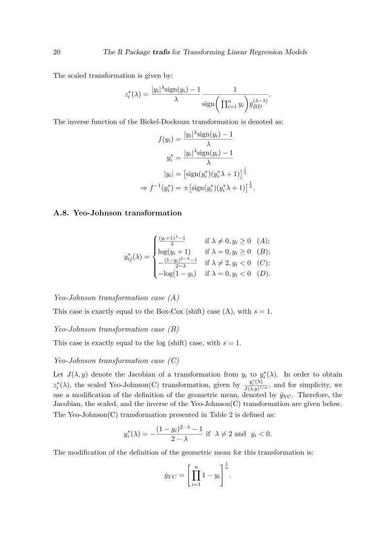
A.8. Yeo-Johnson transformation

y∗ij(λ) =

(yi+1)λ−1

λ if λ 6= 0, yi ≥ 0 (A);

log(yi + 1) if λ = 0, yi ≥ 0 (B);

− (1−yi)2−λ−12−λ if λ 6= 2, yi < 0 (C);

−log(1− yi) if λ = 0, yi < 0 (D).

Yeo-Johnson transformation case (A)

This case is exactly equal to the Box-Cox (shift) case (A), with s = 1.

Yeo-Johnson transformation case (B)

This case is exactly equal to the log (shift) case, with s = 1.

Yeo-Johnson transformation case (C)


z∗i (λ), the scaled Yeo-Johnson(C) transformation, given byy∗i (λ)


use a modification of the definition of the geometric mean, denoted by yYC. Therefore, theJacobian, the scaled, and the inverse of the Yeo-Johnson(C) transformation are given below.

The Yeo-Johnson(C) transformation presented in Table 2 is defined as:

y∗i (λ) = −(1− yi)2−λ − 1

2− λif λ 6= 2 and yi < 0.


yY C =

[n∏i=1

1− yi

] 1n

.



J(λ,y) =n∏i=1

dy∗i (λ)

dy

=n∏i=1

(2− λ)(1− yi)1−λ

2− λ

=n∏i=1

(1− yi)1−λ

= yn(1−λ)Y C .


z∗i (λ) = −(1− yij)2−λ − 1

2− λyn(1−λ)Y C .

The inverse function of the Yeo-Johnson(C) transformation is denoted as:

f(yi) = −(1− yi)2−λ − 1

2− λ

y∗i = −(1− yi)2−λ − 1

2− λ−y∗i (2− λ) = (1− yi)2−λ − 1

yi = 1−[− y∗i (2− λ) + 1

] 12−λ

⇒ f−1(y∗i ) = 1−[− y∗i (2− λ) + 1

] 12−λ .

Yeo-Johnson transformation case (D)

Let J(y) denote the Jacobian of a transformation from yi to y∗i . In order to obtain z∗i ,

the scaled Yeo-Johnson(D) transformation, given byy∗i

J(y)1/n, and for simplicity, we use a

modification of the definition of the geometric mean, denoted by yYD. Therefore, the Jacobian,the scaled, and the inverse of the Yeo-Johnson(D) transformation are given below.

The Yeo-Johnson(D) transformation presented in Table 2 is defined as:

y∗i = − log(1− yi).


yY D =

[n∏i=1

1− yi

] 1n

.


J(λ,y) =

n∏i=1

dy∗idy

=

n∏i=1

1

1− yi= y−nY D.



z∗i = − log(1− yi)yY D.

The inverse function of the Yeo-Johnson(D) transformation is denoted as:

f(yi) = − log(1− yi)y∗i = − log(1− yi)yi = −e−y∗i + 1

⇒ f−1(y∗i ) = −e−y∗i + 1.

A.9. Square root-shift opt transformation


z∗i , the scaled square root-shift opt transformation, given byy∗i (λ)


use a modification of the definition of the geometric mean, denoted by ySR. Therefore, theJacobian, the scaled, and the inverse of the square root-shift opt transformation are givenbelow.

The square root-shift opt transformation presented in Table 2 is defined as:

y∗i (λ) =√yi + λ.


ySR =

[n∏i=1

yi + λ

] 1n

.


J(λ,y) =n∏i=1

dy∗idy

=n∏i=1

− 1

2√yi + λ

=1

2y−n2SR .


z∗i = − 1

yiy2SR.

The inverse function of the square root-shift opt transformation is denoted as:

f(yi) =√yi + λ

y∗i =√yi + λ

yi = y∗2i − λ⇒ f−1(y∗i ) = y∗2i − λ.


A.10. Manly transformation

y∗i (λ) =

{eλyi−1λ if λ 6= 0 (A);

yi if λ = 0 (B).

Manly transformation case (A)


z∗i (λ), the scaled Manly(A) transformation, given byy∗i (λ)

J(λ,y)1/n, and for simplicity, we use a

modification of the definition of the geometric mean, denoted by yM. Therefore, the Jacobian,the scaled, and the inverse of the Manly(A) transformation are given below.

The Manly(A) transformation presented in Table 2 is defined as:

y∗i (λ) =eλyi − 1

λif λ 6= 0.


yM =

[n∏i=1

eyi

] 1n

=[e∑ni=1 yi

] 1n

= ey.


J(λ,y) =

n∏i=1

dy∗i (λ)

dy

=

n∏i=1

λeλyi

λ

=

(n∏i=1

eyi

)λ= yλnM

= eλny.


z∗i (λ) =eλyi − 1

λ

1

yλM

=eλyi − 1

λ

1

eλy.


The inverse function of the Manly(A) transformation is denoted as:

f(yi) =eλyi − 1

λ

y∗i =eλyi − 1

λ

λy∗i + 1 = eλyi

yi =log(λy∗i + 1)

λ

⇒ f−1(y∗i ) =log(λy∗i + 1)

λ.

Manly transformation case (B)

The variable remains equal, y∗i = yi.

A.11. Modulus transformation

y∗i (λ) =

{sign(yi)

(|yi|+1)λ−1λ if λ 6= 0 (A);

sign(yi) log (|yi|+ 1) if λ = 0 (B).

Modulus transformation case (A)


z∗i (λ), the scaled modulos(A) transformation, given byy∗i (λ)

J(λ,y)1/n, and for simplicity, we use

a modification of the definition of the geometric mean, denoted by yMA. Therefore, theJacobian, the scaled, and the inverse of the modulus(A) transformation are given below.

The modulus(A) transformation presented in Table 2 is defined as:

y∗i (λ) = sign(yi)(|yi|+ 1)λ − 1

λif λ 6= 0.


yMA =

[n∏i=1

|yi|+ 1

] 1n

.



J(λ,y) =

n∏i=1

dy∗i (λ)

dy

=n∏i=1

sign(yi)λ(|yi|+ 1)λ−1

λ

= sign

( n∏i=1

yi

)( n∏i=1

|yi|+ 1

)λ−1

= sign

( n∏i=1

yi

)yn(λ−1)MA .


z∗i (λ) = sign(yi)(|yi|+ 1)λ − 1

λ

1

sign

(∏ni=1 yi

)y

(λ−1)MA

.

The inverse function of the modulus(A) transformation is denoted as:

f(yi) = sign(yi)(|yi|+ 1)λ − 1

λ

y∗i = sign(yi)(|yi|+ 1)λ − 1

λ

|yi| =[sign(y∗i )λ+ 1

] 1λ − 1

⇒ f−1(y∗i ) = ±[(

sign(y∗i )λ+ 1) 1λ − 1

].

Modulus transformation case (B)

This case is exactly equal to the neglog transformation case.

A.12. Dual power transformation

y∗i (λ) =

{yλi −y

−λi

2λ if λ > 0 (A);

log(yi) if λ = 0 (B).

Dual power transformation case (A)


z∗i (λ), the scaled dual power(A) transformation, given byy∗i (λ)


use a modification of the definition of the geometric mean, denoted by yDA. Therefore, the


Jacobian, the scaled, and the inverse of the dual power(A) transformation are given below.The dual power(A) transformation presented in Table 2 is defined as:

y∗i (λ) =yλi − y

−λi

2λif λ > 0.


yDA =

[n∏i=1

(yλ−1i + y−λ−1

i

)] 1n

.


J(λ,y) =

n∏i=1

dy∗i (λ)

dy

=

n∏i=1

λyλ−1i + λy−λ−1

i

2λ

=1

2ynDA.


z∗i (λ) =yλi − y

−λi

2λ

2

yDA.

The inverse function of the dual power(A) transformation is found by solving the quadraticby completing the square as:

f(yi) =yλi − y

−λi

2λ

y∗i =yλi − y

−λi

2λ

2λy∗i = yλi − y−λi

2λy∗i = yλi −1

yλi

2λy∗i =y2λi − 1

yλi

2λy∗i yλi = y2λ

i − 1

1 + λ2y∗2i = y2λi − 2λy∗i y

λi + λ2y∗2i

1 + λ2y∗2i = (yλi − λy∗i )2√1 + λ2y∗2i + λy∗i = yλi

yi =[√

1 + λ2y∗2i + λy∗i

] 1λ

⇒ f−1(y∗i ) =[√

1 + λ2y∗2i + λy∗i

] 1λ.


Dual power transformation case (B)

This case is exactly equal to the Box-Cox (shift) transformation, case (B).

A.13. Gpower transformation

y∗i (λ) =

(yi+√y2i+1

)λ−1

λ if λ 6= 0 (A);

log(yi +

√y2i + 1

)if λ = 0 (B).

Gpower transformation case (A)


z∗i (λ), the scaled gpower(A) transformation, given byy∗i (λ)

J(λ,y)1/n, and for simplicity, we use a

modification of the definition of the geometric mean, denoted by yGA. Therefore, the Jacobian,the scaled, and the inverse of the gpower(A) transformation are given below.

The gpower(A) transformation presented in Table 2 is defined as:

y∗i (λ) =

[yi +

√y2i + 1

]λ− 1

λif λ 6= 0.


yGA =

[n∏i=1

(yi +

√y2i + 1

)λ−11 +

yi√y2i + 1

] 1n

.


J(λ,y) =n∏i=1

dy∗i (λ)

dy

=n∏i=1

λ(yi +

√y2i + 1

)λ−1(1 + 2yi

2√y2i+1

)λ

= ynGA.


z∗i (λ) =

[yi +

√y2i + 1

]λ− 1

λ

1

yGA.


The inverse function of the gpower(A) transformation is denoted as:

f(yi) =

[yi +

√y2i + 1

]λ− 1

λ

y∗i =

[yi +

√y2i + 1

]λ− 1

λ

λy∗i + 1 =[yi +

√y2i + 1

]λ(λy∗i + 1)

1λ = yi +

√y2i + 1[

(λy∗i + 1)1λ − yi

]2=[√

y2i + 1

]2

(λy∗i + 1)2λ − 2yi(λy

∗i + 1)

1λ + y2

i = y2i + 1

−yi(λy∗i + 1)1λ =

1− (λy∗i + 1)2λ

2

yi = −

[1− (λy∗i + 1)

2λ

2(λy∗i + 1)1λ

]

⇒ f−1(yi) = −

[1− (λyi + 1)

2λ

2(λyi + 1)1λ

].

Gpower transformation case (B)

This case is exactly equal to the glog transformation case.


References

Bartlett MS (1947). “The use of transformations.” Biometrics, 3(1), 39–52.

Berry WD (1993). Understanding Regression Assumptions. SAGE Publications, ThousandOaks.

Bickel PJ, Doksum KA (1981). “An analysis of transformations revisited.” Journal of theAmerican Statistical Association, 76(374), 296–311.

Box GEP, Cox DR (1964). “An analysis of transformations.” Journal of the Royal StatisticalSociety Series B, 26(2), 211–252.

Breusch TS, Pagan AR (1979). “A simple test for heteroscedasticity and random coefficientvariation.” Econometrica, 47(5), 1287–1294.

Croissant Y (2016). Ecdat: Data Sets for Econometrics. R package version 0.3-1, URLhttps://CRAN.R-project.org/package=Ecdat.

Dag O, Asar O, Ilk O (2017). AID: Box-Cox Power Transformation. R package version 2.3,URL https://CRAN.R-project.org/package=AID.

Durbin BP, Hardin JS, Hawkins DM, Rocke DM (2002). “A variance-stabilizing transforma-tion for gene-expression microarray data.” Bioinformatics, 18(1), 105–110.

Feng Q, Hannig J, Marron JS (2016). “A Note on Automatic Data Transformation.” Stat,5(1), 82–87.

Fernandez ES (2014). Johnson: Johnson Transformation. R package version 1.4, URLhttps://CRAN.R-project.org/package=Johnson.

Fox J, Weisberg S (2011). An R Companion to Applied Regression. SAGE Publications,Thousand Oaks.

Hossain MZ (2011). “The use of Box-Cox transformation technique in economic and statisticalanalyses.” Journal of Emerging Trends in Economics and Management Sciences, 2(1), 32–39.

Hothorn T, Most L, Buhlmann P (2018). “Most likely transformations.” Scandinavian Journalof Statistics, 45(1), 110–134.

John JA, Draper NR (1980). “An alternative family of transformations.” Journal of the RoyalStatistical Society Series C, 29(2), 190–197.

Kelmansky DM, Martınez EJ, Leiva V (2013). “A new variance stabilizing transformation forgene expression data analysis.” Statistical Applications in Genetics and Molecular Biology,12(6), 653–666.

Kuhn M (2008). “Building Predictive Models in R Using the caret Package.” Journal ofStatistical Software, 28(5), 1–26.

https://CRAN.R-project.org/package=Ecdat

https://CRAN.R-project.org/package=AID

https://CRAN.R-project.org/package=Johnson


Manly BFJ (1976). “Exponential data transformations.” Journal of the Royal StatisticalSociety Series D, 25(1), 37–42.

Medina L, Castro P, Kreutzmann AK, Rojas-Perilla N (2018). trafo: Estimation, Com-parison and Selection of Transformations. R package version 1.0.0, URL https://CRAN.

R-project.org/package=trafo.

Molina I, Marhuenda Y (2015). “sae: An R Package for Small Area Estimation.” The R Jour-nal, 7(1), 81–98. URL https://journal.r-project.org/archive/2015/RJ-2015-007/

index.html.

Morozova M, Koschutnig K, Klein E, Wood G (2016). “Monotonic Non-linear Transformationsas a Tool to Investigate Age-related Effects on Brain White Matter Integrity: A Box-CoxInvestigation.” NeuroImage, 125, 1119–1130.

Nelder JA, Wedderburn RWM (1972). “Generalized linear models.” Journal of the RoyalStatistical Society Series A, 135(3), 370–384.

R Core Team (2018). R: A Language and Environment for Statistical Computing. R Founda-tion for Statistical Computing, Vienna. URL https://www.R-project.org/.

Ribeiro Jr PJ, Diggle PJ (2016). “geoR: Analysis of Geostatistical Data.” R News, 1(2),15–18. URL http://cran.R-project.org/doc/Rnews.

Rojas-Perilla N (2018). The Use of Data-Driven Transformations and their Application inSmall Area Estimation. Ph.D. thesis, Freie Universitat Berlin. Unpublished.

Royston P, Lambert PC, et al. (2011). Flexible Parametric Survival Analysis using Stata:Beyond the Cox Model. Stata Press, College Station.

Shapiro SS, Wilk MB (1965). “An Analysis of Variance Test for Normality.” Biometrika,52(3/4), 591–611.

Taylor JMG (1985). “Power transformations to symmetry.” Biometrika, 72(1), 145–152.

Tukey JW (1977). Exploratory Data Analysis. Pearson, London.

Venables WN, Ripley BD (2002). Modern Applied Statistics with S. Springer-Verlag, NewYork.

Wang Y (2015). jtrans: Johnson Transformation for Normality. R package version 1.1.0,URL https://CRAN.R-project.org/package=jtrans.

Whittaker J, Whitehead C, Somers M (2005). “The neglog transformation and quantileregression for the analysis of a large credit scoring database.” Journal of the Royal StatisticalSociety Series C, 54(4), 863–878.

Yang Z (2006). “A modified family of power transformations.” Economics Letters, 92(1),14–19.

Yeo IK, Johnson RA (2000). “A new family of power transformations to improve normalityor symmetry.” Biometrika, 87(4), 954–959.

https://CRAN.R-project.org/package=trafo

https://CRAN.R-project.org/package=trafo

https://journal.r-project.org/archive/2015/RJ-2015-007/index.html

https://journal.r-project.org/archive/2015/RJ-2015-007/index.html

https://www.R-project.org/

http://cran.R-project.org/doc/Rnews

https://CRAN.R-project.org/package=jtrans


Affiliation:

Ann-Kristin KreutzmannInstitute for Statistics and EconometricsFaculty of EconomicsFreie Universitat Berlin14195 Berlin, GermanyE-mail: [email protected]: http://www.wiwiss.fu-berlin.de/fachbereich/vwl/Schmid/Team/Kreutzmann/index.html

mailto:[email protected]

http://www.wiwiss.fu-berlin.de/fachbereich/vwl/Schmid/Team/Kreutzmann/index.html

http://www.wiwiss.fu-berlin.de/fachbereich/vwl/Schmid/Team/Kreutzmann/index.html

Documents

The R Package trafo for Transforming Linear … The R Package trafo for Transforming Linear Regression Models as the log-shift opt, or the Manly transformation, which is an exponential