Embed Size (px)
Citation preview

Model SetupEquilibrium, Planner, Steady State & Dynamics
Government Consumption Spending and DynamicsWays of Financing Government Consumption
The Ramsey ModelLectures 11 to 14
Topics in Macroeconomics
November 10, 11, 24 & 25, 2008
Lecture 11, 12, 13 & 14 1/50 Topics in Macroeconomics
Model SetupEquilibrium, Planner, Steady State & Dynamics
Government Consumption Spending and DynamicsWays of Financing Government Consumption
The Ramsey Model: Introduction 2
Main Ingredients
◮ Neoclassical model of the firm
(Topics 1 & 2)
◮ Consumption-savings choice for consumers
(Topic 3, Certainty)
◮ “Solow model + incentives to save”
(recall example with taxes)
Lecture 11, 12, 13 & 14 2/50 Topics in Macroeconomics
Model SetupEquilibrium, Planner, Steady State & Dynamics
Government Consumption Spending and DynamicsWays of Financing Government Consumption
Model SetupMarkets and OwnershipRepresentative FirmRepresentative Household
Equilibrium, Planner, Steady State & DynamicsDefinition and Characterization of EquilibriumBenevolent Planner’s ProblemSteady StateOff Steady State Dynamics
Government Consumption Spending and DynamicsGovernment Consumption & Lump-Sum TaxesGvmt. Cons, Lump-Sum Taxes: Permanent IncreaseGvmt. Cons, Lump-Sum Taxes: Temporary Increase
Ways of Financing Government ConsumptionRicardian Equivalence: Lump-Sum Taxes vs. DebtDistortionary Taxes on Capital IncomeDistortionary Taxes on Labour Income
Lecture 11, 12, 13 & 14 3/50 Topics in Macroeconomics
Model SetupEquilibrium, Planner, Steady State & Dynamics
Government Consumption Spending and DynamicsWays of Financing Government Consumption
Markets and OwnershipRepresentative FirmRepresentative Household
Model: Markets and ownership 4
Agents◮ Firms produce goods, hire labor and rent capital◮ Households own labor and assets (capital),
receive wages and rental payments, consume and save◮ There are Nt households and many firms
Markets◮ Inputs: competitive wage rates, w , and rental rate, R◮ Assets: free borrowing and lending at interest rate, r◮ Output: competitive market for consumption good
Lecture 11, 12, 13 & 14 4/50 Topics in Macroeconomics
Model SetupEquilibrium, Planner, Steady State & Dynamics
Government Consumption Spending and DynamicsWays of Financing Government Consumption
Markets and OwnershipRepresentative FirmRepresentative Household
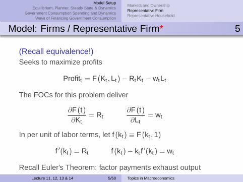
Model: Firms / Representative Firm* 5
(Recall equivalence!)Seeks to maximize profits
Profitt = F (Kt , Lt) − RtKt − wtLt
The FOCs for this problem deliver
∂F (t)∂Kt
= Rt∂F (t)∂Lt
= wt
In per unit of labor terms, let f (kt) ≡ F (kt , 1)
f ′(kt ) = Rt f (kt ) − kt f ′(kt ) = wt
Recall Euler’s Theorem: factor payments exhaust outputLecture 11, 12, 13 & 14 5/50 Topics in Macroeconomics
Model SetupEquilibrium, Planner, Steady State & Dynamics
Government Consumption Spending and DynamicsWays of Financing Government Consumption
Markets and OwnershipRepresentative FirmRepresentative Household
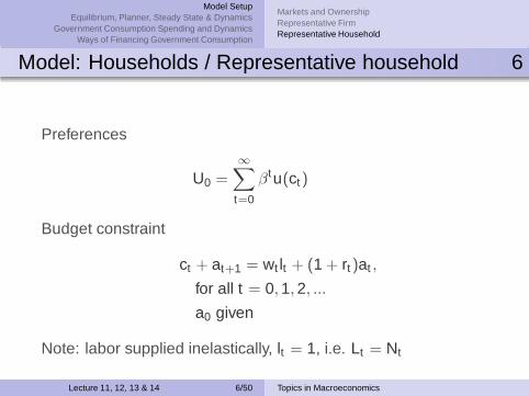
Model: Households / Representative household 6
Preferences
U0 =
∞∑
t=0
βtu(ct)
Budget constraint
ct + at+1 = wt lt + (1 + rt)at ,
for all t = 0, 1, 2, ...
a0 given
Note: labor supplied inelastically, lt = 1, i.e. Lt = Nt
Lecture 11, 12, 13 & 14 6/50 Topics in Macroeconomics
Model SetupEquilibrium, Planner, Steady State & Dynamics
Government Consumption Spending and DynamicsWays of Financing Government Consumption
Markets and OwnershipRepresentative FirmRepresentative Household
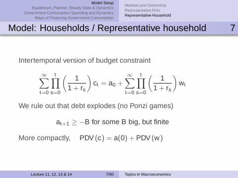
Model: Households / Representative household 7
Intertemporal version of budget constraint
∞∑
t=0
t∏
s=0
(
11 + rs
)
ct = a0 +∞∑
t=0
t∏
s=0
(
11 + rs
)
wt
We rule out that debt explodes (no Ponzi games)
at+1 ≥ −B for some B big, but finite
More compactly, PDV (c) = a(0) + PDV (w)
Lecture 11, 12, 13 & 14 7/50 Topics in Macroeconomics
Model SetupEquilibrium, Planner, Steady State & Dynamics
Government Consumption Spending and DynamicsWays of Financing Government Consumption
Markets and OwnershipRepresentative FirmRepresentative Household
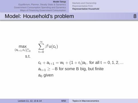
Model: Household’s problem 8
max(at+1,ct )
∞
t=0
∞∑
t=0
βtu(ct)
s.t.
ct + at+1 = wt + (1 + rt)at , for all t = 0, 1, 2, ...
at+1 ≥ −B for some B big, but finite
a0 given
Lecture 11, 12, 13 & 14 8/50 Topics in Macroeconomics
Model SetupEquilibrium, Planner, Steady State & Dynamics
Government Consumption Spending and DynamicsWays of Financing Government Consumption
Markets and OwnershipRepresentative FirmRepresentative Household
Model: Household’s problem 9
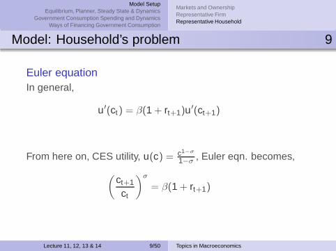
Euler equationIn general,
u′(ct) = β(1 + rt+1)u′(ct+1)
From here on, CES utility, u(c) = c1−σ
1−σ , Euler eqn. becomes,
(
ct+1
ct
)σ
= β(1 + rt+1)
Lecture 11, 12, 13 & 14 9/50 Topics in Macroeconomics
Model SetupEquilibrium, Planner, Steady State & Dynamics
Government Consumption Spending and DynamicsWays of Financing Government Consumption
Markets and OwnershipRepresentative FirmRepresentative Household
Model: Household’s problem 10
Budget constraint
ct + at+1 = wt + (1 + rt)at , for all t = 0, 1, 2, ...
Lecture 11, 12, 13 & 14 10/50 Topics in Macroeconomics
Model SetupEquilibrium, Planner, Steady State & Dynamics
Government Consumption Spending and DynamicsWays of Financing Government Consumption
Markets and OwnershipRepresentative FirmRepresentative Household
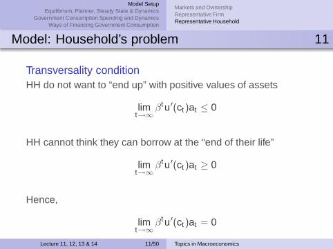
Model: Household’s problem 11
Transversality conditionHH do not want to “end up” with positive values of assets
limt→∞
βtu′(ct)at ≤ 0
HH cannot think they can borrow at the “end of their life”
limt→∞
βtu′(ct)at ≥ 0
Hence,
limt→∞
βtu′(ct)at = 0
Lecture 11, 12, 13 & 14 11/50 Topics in Macroeconomics
Model SetupEquilibrium, Planner, Steady State & Dynamics
Government Consumption Spending and DynamicsWays of Financing Government Consumption
Definition and Characterization of EquilibriumBenevolent Planner’s ProblemSteady StateOff Steady State Dynamics
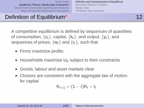
Definition of Equilibrium* 12
A competitive equilibrium is defined by sequences of quantitiesof consumption, {ct}, capital, {kt}, and output, {yt}, andsequences of prices, {wt} and {rt}, such that
◮ Firms maximize profits
◮ Households maximize U0 subject to their constraints
◮ Goods, labour and asset markets clear◮ Choices are consistent with the aggregate law of motion
for capitalKt+1 = (1 − δ)Kt + It
Lecture 11, 12, 13 & 14 12/50 Topics in Macroeconomics

Model SetupEquilibrium, Planner, Steady State & Dynamics
Government Consumption Spending and DynamicsWays of Financing Government Consumption
Definition and Characterization of EquilibriumBenevolent Planner’s ProblemSteady StateOff Steady State Dynamics
Characterizing Equilibrium Quantities* 13
From the equilibrium conditions derived before, we find:
◮ There cannot be arbitrage opportunities in equilibrium
Rt − δ = rt
In equilibrium it does not pay to invest in capital directly.The riskless asset and capital have the same payoff.
Lecture 11, 12, 13 & 14 13/50 Topics in Macroeconomics
Model SetupEquilibrium, Planner, Steady State & Dynamics
Government Consumption Spending and DynamicsWays of Financing Government Consumption
Definition and Characterization of EquilibriumBenevolent Planner’s ProblemSteady StateOff Steady State Dynamics
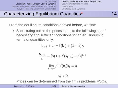
Characterizing Equilibrium Quantities* 14
From the equilibrium conditions derived before, we find:
◮ Substituting out all the prices leads to the following set ofnecessary and sufficient conditions for an equilibrium interms of quantities only.
kt+1 + ct = f (kt) + (1 − δ)kt
ct+1
ct= [β(1 + f ′(kt+1) − δ)]1/σ
limt→∞
βtu′(ct )kt = 0
k0 > 0
Prices can be determined from the firm’s problems FOCs.Lecture 11, 12, 13 & 14 14/50 Topics in Macroeconomics
Model SetupEquilibrium, Planner, Steady State & Dynamics
Government Consumption Spending and DynamicsWays of Financing Government Consumption
Definition and Characterization of EquilibriumBenevolent Planner’s ProblemSteady StateOff Steady State Dynamics
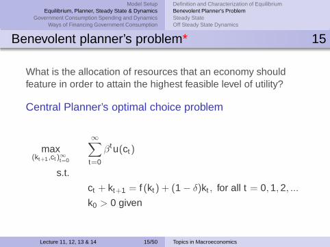
Benevolent planner’s problem* 15
What is the allocation of resources that an economy shouldfeature in order to attain the highest feasible level of utility?
Central Planner’s optimal choice problem
max(kt+1,ct)
∞
t=0
∞∑
t=0
βtu(ct)
s.t.
ct + kt+1 = f (kt) + (1 − δ)kt , for all t = 0, 1, 2, ...
k0 > 0 given
Lecture 11, 12, 13 & 14 15/50 Topics in Macroeconomics
Model SetupEquilibrium, Planner, Steady State & Dynamics
Government Consumption Spending and DynamicsWays of Financing Government Consumption
Definition and Characterization of EquilibriumBenevolent Planner’s ProblemSteady StateOff Steady State Dynamics
Benevolent planner’s problem 16
Welfare
Socially optimal allocation coincides with the equilibriumallocation.
The competitive equilibrium leads to the social optimum.
Not surprising: no distortions or externalities→ Welfare Theorems hold
Lecture 11, 12, 13 & 14 16/50 Topics in Macroeconomics
Model SetupEquilibrium, Planner, Steady State & Dynamics
Government Consumption Spending and DynamicsWays of Financing Government Consumption
Definition and Characterization of EquilibriumBenevolent Planner’s ProblemSteady StateOff Steady State Dynamics
Notes: simplifying features* 17
◮ We are considering an economy without population growth.
◮ There is no exogenous technological change, either.
Lecture 11, 12, 13 & 14 17/50 Topics in Macroeconomics
Model SetupEquilibrium, Planner, Steady State & Dynamics
Government Consumption Spending and DynamicsWays of Financing Government Consumption
Definition and Characterization of EquilibriumBenevolent Planner’s ProblemSteady StateOff Steady State Dynamics
Steady state* 18
Definition
A balanced growth path (BGP) is a situation in which output,capital and consumption grow at a constant rate.
If this constant rate is zero, it is called a steady state.
We can usually redefine the state variable so that the latter isconstant (i.e. the growth rate is zero)
Recall from the Solow model:
aggregate capital stock for (n = 0, g = 0)capital per unit of labor for (n > 0, g = 0)capital per unit of effective labor for (n > 0, g > 0)
Lecture 11, 12, 13 & 14 18/50 Topics in Macroeconomics

Model SetupEquilibrium, Planner, Steady State & Dynamics
Government Consumption Spending and DynamicsWays of Financing Government Consumption
Definition and Characterization of EquilibriumBenevolent Planner’s ProblemSteady StateOff Steady State Dynamics
Steady state 19
From the Euler equation,
ct+1
ct= [β(1 + f ′(kt+1) − δ)]1/σ , for all t
If consumption grows at a constant rate (BGP), say γ
1 + γ = [β(1 + f ′(kt+1) − δ)]1/σ , for all t
Thus RHS must be constant→ kt+1 = kt = k∗ must be constant along the BGP
Lecture 11, 12, 13 & 14 19/50 Topics in Macroeconomics
Model SetupEquilibrium, Planner, Steady State & Dynamics
Government Consumption Spending and DynamicsWays of Financing Government Consumption
Definition and Characterization of EquilibriumBenevolent Planner’s ProblemSteady StateOff Steady State Dynamics
Steady state 20
But then, from the resource constraint with kt = kt+1 = k∗:
ct + kt+1 = f (kt) + (1 − δ)kt , for all t
i.e.,ct = f (k∗) − δk∗
ct+1 = f (k∗) − δk∗
We find that consumption must be constant along the BGP,→ ct+1 = ct = c∗ or γ = 0
Hence we have a steady state in per capita variables.
Lecture 11, 12, 13 & 14 20/50 Topics in Macroeconomics
Model SetupEquilibrium, Planner, Steady State & Dynamics
Government Consumption Spending and DynamicsWays of Financing Government Consumption
Definition and Characterization of EquilibriumBenevolent Planner’s ProblemSteady StateOff Steady State Dynamics
Steady state* 21
Hence from the Euler equation
1 + γ = 1 = [β(1 + f ′(k∗) − δ)]1/σ
or, simplified
f ′(k∗) =1β− (1 − δ) = ρ + δ
we can solve for k∗and from the (simplified) resource constraint
c∗ = f (k∗) − δk∗
we can solve for c∗
Lecture 11, 12, 13 & 14 21/50 Topics in Macroeconomics
Model SetupEquilibrium, Planner, Steady State & Dynamics
Government Consumption Spending and DynamicsWays of Financing Government Consumption
Definition and Characterization of EquilibriumBenevolent Planner’s ProblemSteady StateOff Steady State Dynamics
Modified golden rule* 22
The capital stock that maximizes utility in steady state is calledthe modified golden rule level of capital
f ′(k∗) = ρ + δ
Using f (k) = kα, we get
k∗ = kMGR =
[
α
ρ + δ
]1
1−α
Compare to golden rule level of capital(max conso in st. st.)
kGR =[α
δ
]1
1−α
(see Problem set 2, Q 2.2, assume A = 1 and set s = α)Lecture 11, 12, 13 & 14 22/50 Topics in Macroeconomics
Model SetupEquilibrium, Planner, Steady State & Dynamics
Government Consumption Spending and DynamicsWays of Financing Government Consumption
Definition and Characterization of EquilibriumBenevolent Planner’s ProblemSteady StateOff Steady State Dynamics
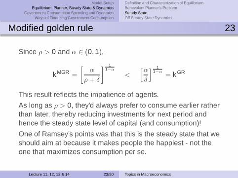
Modified golden rule 23
Since ρ > 0 and α ∈ (0, 1),
kMGR =
[
α
ρ + δ
]1
1−α
<[α
δ
]1
1−α
= kGR
This result reflects the impatience of agents.
As long as ρ > 0, they’d always prefer to consume earlier ratherthan later, thereby reducing investments for next period andhence the steady state level of capital (and consumption)!
One of Ramsey’s points was that this is the steady state that weshould aim at because it makes people the happiest - not theone that maximizes consumption per se.
Lecture 11, 12, 13 & 14 23/50 Topics in Macroeconomics
Model SetupEquilibrium, Planner, Steady State & Dynamics
Government Consumption Spending and DynamicsWays of Financing Government Consumption
Definition and Characterization of EquilibriumBenevolent Planner’s ProblemSteady StateOff Steady State Dynamics
Off steady state dynamics* 24
Off the steady state, consumption and capital adjust to reachthe steady state eventually.
To analyze these dynamics, consider the movements of c and kseparately.
Let ∆c = ct+1 − ct and ∆k = kt+1 − kt . See graphical analysis.
Lecture 11, 12, 13 & 14 24/50 Topics in Macroeconomics
Model SetupEquilibrium, Planner, Steady State & Dynamics
Government Consumption Spending and DynamicsWays of Financing Government Consumption
Definition and Characterization of EquilibriumBenevolent Planner’s ProblemSteady StateOff Steady State Dynamics
Off steady state dynamics* 25
We use 2 equilibrium conditions:
◮ Euler equation (EE)
ct+1
ct= [β(1 + f ′(kt+1) − δ)]1/σ
◮ Resource constraint (RC)
ct + kt+1 = f (kt) + (1 − δ)kt
Lecture 11, 12, 13 & 14 25/50 Topics in Macroeconomics
Model SetupEquilibrium, Planner, Steady State & Dynamics
Government Consumption Spending and DynamicsWays of Financing Government Consumption
Definition and Characterization of EquilibriumBenevolent Planner’s ProblemSteady StateOff Steady State Dynamics
Off steady state dynamics* 26
◮ Let ∆c = ct+1 − ct and ∆k = kt+1 − kt
◮ Use EE to determine points where ∆c = 0
◮ Use RC to determine points where ∆k = 0
◮ Look at dynamics left and right of ∆c = 0
◮ Look at dynamics above and below ∆k = 0
◮ Steady state is where ∆c = 0 and ∆k = 0
Lecture 11, 12, 13 & 14 26/50 Topics in Macroeconomics
Model SetupEquilibrium, Planner, Steady State & Dynamics
Government Consumption Spending and DynamicsWays of Financing Government Consumption
Definition and Characterization of EquilibriumBenevolent Planner’s ProblemSteady StateOff Steady State Dynamics
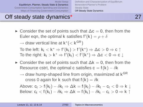
Off steady state dynamics* 27
◮ Consider the set of points such that ∆c = 0, then from theEuler eqn, the optimal k satisfies f ′(k) = ρ + δ
→ draw vertical line at k∗(< kGR)
To the left: kt < k∗ ⇒ f ′(kt) > f ′(k∗) ⇒ ∆c > 0 ⇒ c ↑To the right: kt > k∗ ⇒ f ′(kt) < f ′(k∗) ⇒ ∆c < 0 ⇒ c ↓
◮ Consider the set of points such that ∆k = 0, then from theResource cstrt, the optimal c satisfies c = f (k) − δk
→ draw hump-shaped line from origin, maximized at kGR
cross 0 again for k such that f (k) = δk
Above: ct > f (kt) − δkt ⇒ ∆k = f (kt ) − δkt − ct < 0 ⇒ k ↓Below: ct < f (kt) − δkt ⇒ ∆k = f (kt) − δkt − ct > 0 ⇒ k ↑
Lecture 11, 12, 13 & 14 27/50 Topics in Macroeconomics
Model SetupEquilibrium, Planner, Steady State & Dynamics
Government Consumption Spending and DynamicsWays of Financing Government Consumption
Definition and Characterization of EquilibriumBenevolent Planner’s ProblemSteady StateOff Steady State Dynamics
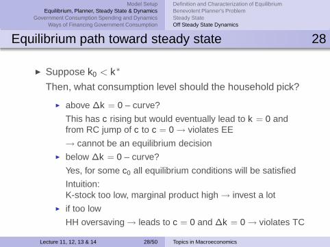
Equilibrium path toward steady state 28
◮ Suppose k0 < k∗
Then, what consumption level should the household pick?
◮ above ∆k = 0 – curve?
This has c rising but would eventually lead to k = 0 andfrom RC jump of c to c = 0 → violates EE
→ cannot be an equilibrium decision◮ below ∆k = 0 – curve?
Yes, for some c0 all equilibrium conditions will be satisfied
Intuition:K-stock too low, marginal product high → invest a lot
◮ if too low
HH oversaving → leads to c = 0 and ∆k = 0 → violates TC
Lecture 11, 12, 13 & 14 28/50 Topics in Macroeconomics
Model SetupEquilibrium, Planner, Steady State & Dynamics
Government Consumption Spending and DynamicsWays of Financing Government Consumption
Definition and Characterization of EquilibriumBenevolent Planner’s ProblemSteady StateOff Steady State Dynamics
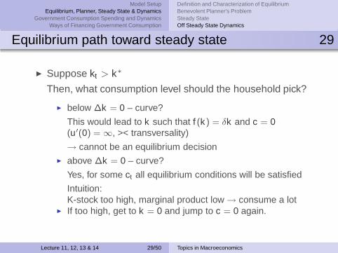
Equilibrium path toward steady state 29
◮ Suppose kt > k∗
Then, what consumption level should the household pick?
◮ below ∆k = 0 – curve?
This would lead to k such that f (k) = δk and c = 0(u′(0) = ∞, >< transversality)
→ cannot be an equilibrium decision◮ above ∆k = 0 – curve?
Yes, for some ct all equilibrium conditions will be satisfied
Intuition:K-stock too high, marginal product low → consume a lot
◮ If too high, get to k = 0 and jump to c = 0 again.
Lecture 11, 12, 13 & 14 29/50 Topics in Macroeconomics
Model SetupEquilibrium, Planner, Steady State & Dynamics
Government Consumption Spending and DynamicsWays of Financing Government Consumption
Government Consumption & Lump-Sum TaxesGvmt. Cons, Lump-Sum Taxes: Permanent IncreaseGvmt. Cons, Lump-Sum Taxes: Temporary Increase
Fiscal policy (Romer 1996 p.59–72) 30
→ Government cons. spending (per capita), gt
→ Financed by lump-sum taxes τt borne by households
The main modifications to the model are:
◮ Public sector
τt = gt , for all t = 0, 1, 2, ...
◮ Household pays taxes
ct + at+1 = wt + (1 + rt)at − τt , for all t = 0, 1, 2, ...
Lecture 11, 12, 13 & 14 30/50 Topics in Macroeconomics
Model SetupEquilibrium, Planner, Steady State & Dynamics
Government Consumption Spending and DynamicsWays of Financing Government Consumption
Government Consumption & Lump-Sum TaxesGvmt. Cons, Lump-Sum Taxes: Permanent IncreaseGvmt. Cons, Lump-Sum Taxes: Temporary Increase
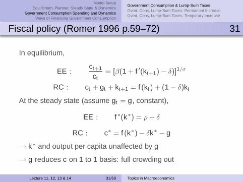
Fiscal policy (Romer 1996 p.59–72) 31
In equilibrium,
EE :ct+1
ct= [β(1 + f ′(kt+1) − δ)]1/σ
RC : ct + gt + kt+1 = f (kt) + (1 − δ)kt
At the steady state (assume gt = g, constant),
EE : f ∗(k∗) = ρ + δ
RC : c∗ = f (k∗) − δk∗ − g
→ k∗ and output per capita unaffected by g
→ g reduces c on 1 to 1 basis: full crowding out
Lecture 11, 12, 13 & 14 31/50 Topics in Macroeconomics
Model SetupEquilibrium, Planner, Steady State & Dynamics
Government Consumption Spending and DynamicsWays of Financing Government Consumption
Government Consumption & Lump-Sum TaxesGvmt. Cons, Lump-Sum Taxes: Permanent IncreaseGvmt. Cons, Lump-Sum Taxes: Temporary Increase
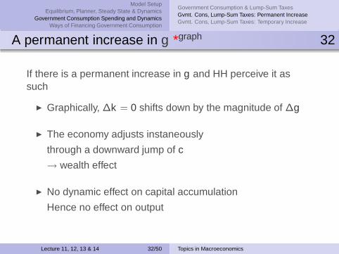
A permanent increase in g *graph 32
If there is a permanent increase in g and HH perceive it assuch
◮ Graphically, ∆k = 0 shifts down by the magnitude of ∆g
◮ The economy adjusts instaneously
through a downward jump of c
→ wealth effect
◮ No dynamic effect on capital accumulation
Hence no effect on output
Lecture 11, 12, 13 & 14 32/50 Topics in Macroeconomics
Model SetupEquilibrium, Planner, Steady State & Dynamics
Government Consumption Spending and DynamicsWays of Financing Government Consumption
Government Consumption & Lump-Sum TaxesGvmt. Cons, Lump-Sum Taxes: Permanent IncreaseGvmt. Cons, Lump-Sum Taxes: Temporary Increase
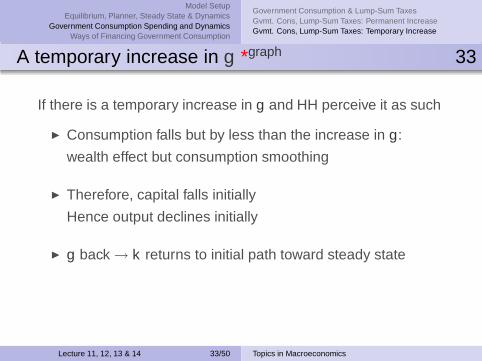
A temporary increase in g *graph 33
If there is a temporary increase in g and HH perceive it as such
◮ Consumption falls but by less than the increase in g:
wealth effect but consumption smoothing
◮ Therefore, capital falls initially
Hence output declines initially
◮ g back → k returns to initial path toward steady state
Lecture 11, 12, 13 & 14 33/50 Topics in Macroeconomics
Model SetupEquilibrium, Planner, Steady State & Dynamics
Government Consumption Spending and DynamicsWays of Financing Government Consumption
Government Consumption & Lump-Sum TaxesGvmt. Cons, Lump-Sum Taxes: Permanent IncreaseGvmt. Cons, Lump-Sum Taxes: Temporary Increase
First conclusions 34
Government spending cannot increase the steady state level ofoutput per capita.
It can even decrease it in the short–run,e.g. when changes are temporary.
Lecture 11, 12, 13 & 14 34/50 Topics in Macroeconomics
Model SetupEquilibrium, Planner, Steady State & Dynamics
Government Consumption Spending and DynamicsWays of Financing Government Consumption
Ricardian Equivalence: Lump-Sum Taxes vs. DebtDistortionary Taxes on Capital IncomeDistortionary Taxes on Labour Income
Ricardian equivalence: lump sum taxes vs. debt 35
Does it matter whether the government chooses to finance
expenditures through debt or non distortionary taxes?
Two approaches:
Lecture 11, 12, 13 & 14 35/50 Topics in Macroeconomics
Model SetupEquilibrium, Planner, Steady State & Dynamics
Government Consumption Spending and DynamicsWays of Financing Government Consumption
Ricardian Equivalence: Lump-Sum Taxes vs. DebtDistortionary Taxes on Capital IncomeDistortionary Taxes on Labour Income
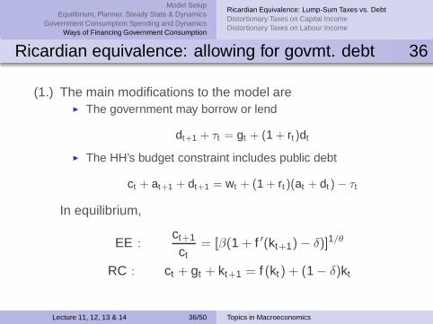
Ricardian equivalence: allowing for govmt. debt 36
(1.) The main modifications to the model are◮ The government may borrow or lend
dt+1 + τt = gt + (1 + rt)dt
◮ The HH’s budget constraint includes public debt
ct + at+1 + dt+1 = wt + (1 + rt )(at + dt ) − τt
In equilibrium,
EE :ct+1
ct= [β(1 + f ′(kt+1) − δ)]1/θ
RC : ct + gt + kt+1 = f (kt) + (1 − δ)kt
Lecture 11, 12, 13 & 14 36/50 Topics in Macroeconomics
Model SetupEquilibrium, Planner, Steady State & Dynamics
Government Consumption Spending and DynamicsWays of Financing Government Consumption
Ricardian Equivalence: Lump-Sum Taxes vs. DebtDistortionary Taxes on Capital IncomeDistortionary Taxes on Labour Income
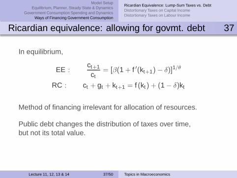
Ricardian equivalence: allowing for govmt. debt 37
In equilibrium,
EE :ct+1
ct= [β(1 + f ′(kt+1) − δ)]1/θ
RC : ct + gt + kt+1 = f (kt) + (1 − δ)kt
Method of financing irrelevant for allocation of resources.
Public debt changes the distribution of taxes over time,but not its total value.
Lecture 11, 12, 13 & 14 37/50 Topics in Macroeconomics
Model SetupEquilibrium, Planner, Steady State & Dynamics
Government Consumption Spending and DynamicsWays of Financing Government Consumption
Ricardian Equivalence: Lump-Sum Taxes vs. DebtDistortionary Taxes on Capital IncomeDistortionary Taxes on Labour Income
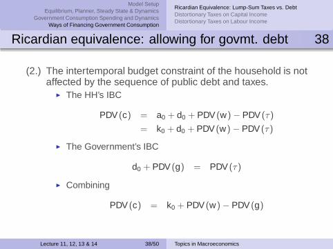
Ricardian equivalence: allowing for govmt. debt 38
(2.) The intertemporal budget constraint of the household is notaffected by the sequence of public debt and taxes.
◮ The HH’s IBC
PDV (c) = a0 + d0 + PDV (w) − PDV (τ)
= k0 + d0 + PDV (w) − PDV (τ)
◮ The Government’s IBC
d0 + PDV (g) = PDV (τ)
◮ Combining
PDV (c) = k0 + PDV (w) − PDV (g)
Lecture 11, 12, 13 & 14 38/50 Topics in Macroeconomics
Model SetupEquilibrium, Planner, Steady State & Dynamics
Government Consumption Spending and DynamicsWays of Financing Government Consumption
Ricardian Equivalence: Lump-Sum Taxes vs. DebtDistortionary Taxes on Capital IncomeDistortionary Taxes on Labour Income
Ricardian equivalence: allowing for govmt. debt 39
PDV (c) = k0 + PDV (w)− PDV (g)
All that matters for household’s behaviour is the present valueof government expenditures, irrespective of how thegovernment decides to pay for it.
Lecture 11, 12, 13 & 14 39/50 Topics in Macroeconomics
Model SetupEquilibrium, Planner, Steady State & Dynamics
Government Consumption Spending and DynamicsWays of Financing Government Consumption
Ricardian Equivalence: Lump-Sum Taxes vs. DebtDistortionary Taxes on Capital IncomeDistortionary Taxes on Labour Income
Key assumptions for Ricardian equivalence to hold 40
The debate on Ricardian equivalence:
◮ Infinite horizon OR OLG framework
◮ Perfect capital markets → liquidity constraints
◮ Lump-sum taxation → distortionary taxes: next
◮ Full rationality → rule of thumb?
are key assumptions underlying Ricardian
Lecture 11, 12, 13 & 14 40/50 Topics in Macroeconomics
Model SetupEquilibrium, Planner, Steady State & Dynamics
Government Consumption Spending and DynamicsWays of Financing Government Consumption
Ricardian Equivalence: Lump-Sum Taxes vs. DebtDistortionary Taxes on Capital IncomeDistortionary Taxes on Labour Income
Distortionary taxes on capital income 41
Tax rate on capital income, τk , with receipts being used tofinance government consumption, g.
The main modifications to the basic model are:
◮ Government’s budget constraint
τkt rtat = gt
◮ Household’s budget constraint
ct + at+1 = wt + (1 + (1 − τkt)rt )at
The tax rate influences the after-tax rate of return on savings.
Lecture 11, 12, 13 & 14 41/50 Topics in Macroeconomics
Model SetupEquilibrium, Planner, Steady State & Dynamics
Government Consumption Spending and DynamicsWays of Financing Government Consumption
Ricardian Equivalence: Lump-Sum Taxes vs. DebtDistortionary Taxes on Capital IncomeDistortionary Taxes on Labour Income
Distortionary taxes on capital income 42
The Euler equation becomes:
EE :ct+1
ct= [β(1 + (1 − τkt+1)rt+1)]
1/θ
In equilibrium,
EE :ct+1
ct= [β(1 + (1 − τkt+1)(f
′(kt+1) − δ)]1/θ
RC : ct + gt + kt+1 = f (kt) + (1 − δ)kt
in addition to k0 > 0 and the transversality condition.
Notice that now the EE changes, hence the intertemporalconsumption-savings decision is distorted.
Lecture 11, 12, 13 & 14 42/50 Topics in Macroeconomics
Model SetupEquilibrium, Planner, Steady State & Dynamics
Government Consumption Spending and DynamicsWays of Financing Government Consumption
Ricardian Equivalence: Lump-Sum Taxes vs. DebtDistortionary Taxes on Capital IncomeDistortionary Taxes on Labour Income
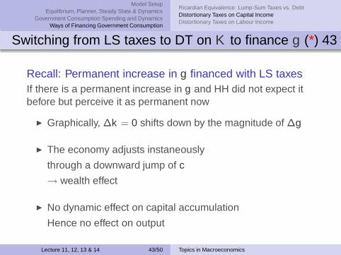
Switching from LS taxes to DT on K to finance g (*) 43
Recall: Permanent increase in g financed with LS taxesIf there is a permanent increase in g and HH did not expect itbefore but perceive it as permanent now
◮ Graphically, ∆k = 0 shifts down by the magnitude of ∆g
◮ The economy adjusts instaneously
through a downward jump of c
→ wealth effect
◮ No dynamic effect on capital accumulation
Hence no effect on output
Lecture 11, 12, 13 & 14 43/50 Topics in Macroeconomics
Model SetupEquilibrium, Planner, Steady State & Dynamics
Government Consumption Spending and DynamicsWays of Financing Government Consumption
Ricardian Equivalence: Lump-Sum Taxes vs. DebtDistortionary Taxes on Capital IncomeDistortionary Taxes on Labour Income
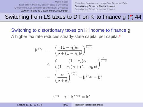
Switching from LS taxes to DT on K to finance g (*) 44
Switching to distortionary taxes on K income to finance gA higher tax rate reduces steady-state capital per capita.*
k∗τk =
(
(1 − τk )α
ρ + (1 − τk )δ
)1
1−α
<
(
(1 − τk )α
(1 − τk )ρ + (1 − τk)δ
)1
1−α
=
(
α
ρ + δ
)1
1−α
= k∗τLS = k∗
k∗τk < k∗τLS = k∗
Lecture 11, 12, 13 & 14 44/50 Topics in Macroeconomics
Model SetupEquilibrium, Planner, Steady State & Dynamics
Government Consumption Spending and DynamicsWays of Financing Government Consumption
Ricardian Equivalence: Lump-Sum Taxes vs. DebtDistortionary Taxes on Capital IncomeDistortionary Taxes on Labour Income
Switching from LS taxes to DT on K to finance g (*) 45
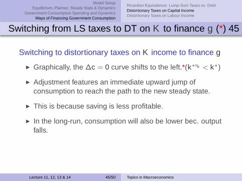
Switching to distortionary taxes on K income to finance g
◮ Graphically, the ∆c = 0 curve shifts to the left.*(k∗τk < k∗)
◮ Adjustment features an immediate upward jump ofconsumption to reach the path to the new steady state.
◮ This is because saving is less profitable.
◮ In the long-run, consumption will also be lower bec. outputfalls.
Lecture 11, 12, 13 & 14 45/50 Topics in Macroeconomics
Model SetupEquilibrium, Planner, Steady State & Dynamics
Government Consumption Spending and DynamicsWays of Financing Government Consumption
Ricardian Equivalence: Lump-Sum Taxes vs. DebtDistortionary Taxes on Capital IncomeDistortionary Taxes on Labour Income
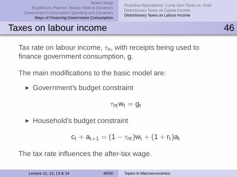
Taxes on labour income 46
Tax rate on labour income, τn, with receipts being used tofinance government consumption, g.
The main modifications to the basic model are:
◮ Government’s budget constraint
τntwt = gt
◮ Household’s budget constraint
ct + at+1 = (1 − τnt)wt + (1 + rt)at
The tax rate influences the after-tax wage.
Lecture 11, 12, 13 & 14 46/50 Topics in Macroeconomics
Model SetupEquilibrium, Planner, Steady State & Dynamics
Government Consumption Spending and DynamicsWays of Financing Government Consumption
Ricardian Equivalence: Lump-Sum Taxes vs. DebtDistortionary Taxes on Capital IncomeDistortionary Taxes on Labour Income
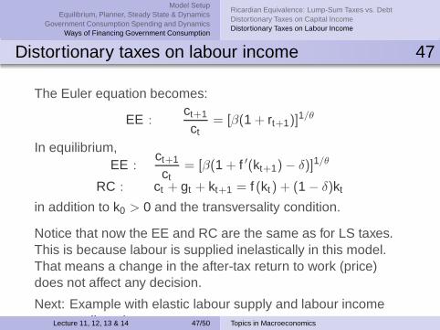
Distortionary taxes on labour income 47
The Euler equation becomes:
EE :ct+1
ct= [β(1 + rt+1)]
1/θ
In equilibrium,EE :
ct+1
ct= [β(1 + f ′(kt+1) − δ)]1/θ
RC : ct + gt + kt+1 = f (kt) + (1 − δ)kt
in addition to k0 > 0 and the transversality condition.
Notice that now the EE and RC are the same as for LS taxes.This is because labour is supplied inelastically in this model.That means a change in the after-tax return to work (price)does not affect any decision.
Next: Example with elastic labour supply and labour incometaxes → distortionLecture 11, 12, 13 & 14 47/50 Topics in Macroeconomics
Model SetupEquilibrium, Planner, Steady State & Dynamics
Government Consumption Spending and DynamicsWays of Financing Government Consumption
Ricardian Equivalence: Lump-Sum Taxes vs. DebtDistortionary Taxes on Capital IncomeDistortionary Taxes on Labour Income
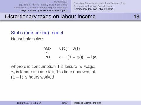
Distortionary taxes on labour income 48
Static (one period) modelHousehold solves
maxc,l
u(c) + v(l)
s.t. c = (1 − τn)(1 − l)w
where c is consumption, l is leisure, w wage,τn is labour income tax, 1 is time endowment,(1 − l) is hours worked
Lecture 11, 12, 13 & 14 48/50 Topics in Macroeconomics
Model SetupEquilibrium, Planner, Steady State & Dynamics
Government Consumption Spending and DynamicsWays of Financing Government Consumption
Ricardian Equivalence: Lump-Sum Taxes vs. DebtDistortionary Taxes on Capital IncomeDistortionary Taxes on Labour Income
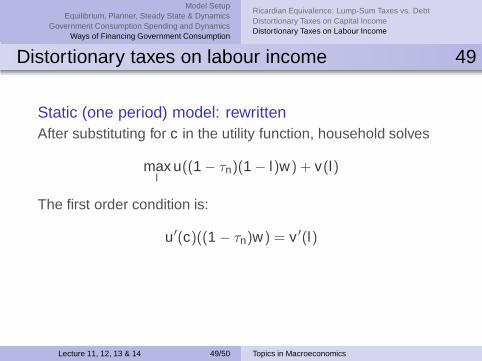
Distortionary taxes on labour income 49
Static (one period) model: rewrittenAfter substituting for c in the utility function, household solves
maxl
u((1 − τn)(1 − l)w) + v(l)
The first order condition is:
u′(c)((1 − τn)w) = v ′(l)
Lecture 11, 12, 13 & 14 49/50 Topics in Macroeconomics
Model SetupEquilibrium, Planner, Steady State & Dynamics
Government Consumption Spending and DynamicsWays of Financing Government Consumption
Ricardian Equivalence: Lump-Sum Taxes vs. DebtDistortionary Taxes on Capital IncomeDistortionary Taxes on Labour Income
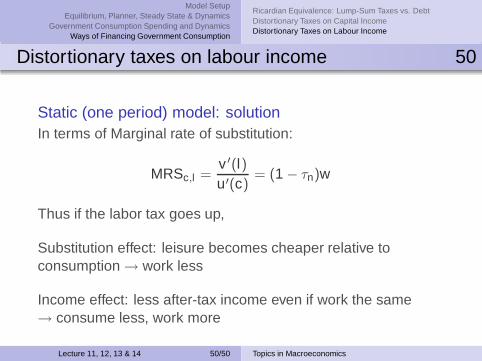
Distortionary taxes on labour income 50
Static (one period) model: solutionIn terms of Marginal rate of substitution:
MRSc,l =v ′(l)u′(c)
= (1 − τn)w
Thus if the labor tax goes up,
Substitution effect: leisure becomes cheaper relative toconsumption → work less
Income effect: less after-tax income even if work the same→ consume less, work more
Lecture 11, 12, 13 & 14 50/50 Topics in Macroeconomics