The Randall-Sundrum Model

Maxime Gabella

June 2006

IPPC, EPFL

Abstract

The Randall-Sundrum model was conceived in 1999 to address theHiggs Hierarchy Problem in particle physics. It arose enormous inter-est from theoreticians and phenomenologists ever since and revealed afruitful tool to explore the physics of extra dimensions. The aim of thispaper is to provide an introductory exposition of this model. After ashort survey of Kaluza-Klein theories, the setup of the RS model willbe exposed and its metric derived. We will explain how an exponentialhierarchy between the gravity scale and the weak scale can be natu-rally generated, and how the standard 4D gravity emerges from thismodel in the Newtonian limit. The Golberger-Wise mechanism willbe presented as a way to stabilize the radius of the extra dimensionwithout reintroducing a fine-tuning. Those topics will be presented inan utterly pedagogical way. Here you will find what textbooks feel freeto disregard as too advanced but research papers consider as too basicto even be mentioned.

1

Contents

1 Basics of Kaluza-Klein theories 3

2 Setup 5

3 Warped metric 5

4 Exponential hierarchy 9

5 Graviton modes 11

6 Graviton spectrum 17

7 Newtonian limit 18

8 Radius stabilization 21

A Einstein tensor 25

2

1 Basics of Kaluza-Klein theories

The existence of extra dimensions of space was first put forth in the middleof the 1920’s by Theodor Kaluza and Oskar Klein [1] as a means of unifyingthe electromagnetic and gravitational fields as components of a single higher-dimensional field. As an illustration, consider the case of a five-dimensionaltheory, with the extra dimension periodically identified:

x5 ∼ x5 + 2πR.

This procedure is called toroidal compactification [2]. The space obtainedis the product of the traditional four-dimensional Minkowski space with acircle, noted M4 ⊗ S1, which can be imagined as a 5D cylinder of radius R.In such a theory, a massless scalar field φ(xµ, x5) would have a quantizedmomentum in the periodic dimension:

p5 =n

R,

with n ∈ Z. We may then expand the field in Fourier series:

φ(xµ, x5) =∞∑

n=−∞φn(xµ)ei

nR

x5.

With this decomposition, the five-dimensional equation of motions (∂µ∂µ +

∂5∂5)φ = 0 becomes

∂µ∂µφn(xµ) =

n2

R2φn(xµ).

In this way, an infinite tower of fields with masses m2 = n2/R2 is generated.At energies small compared to R−1, only the x5-independent massless zero-mode remains and the physics is effectively four-dimensional. At energiesabove R−1, the tower of Kaluza-Klein (KK) states comes into play.

An experimental bound on the size of the compactification radius R isimposed by the fact that those KK states have not been detected at collidersup to TeV energies. Their masses would thus have to be greater, n/R >TeV,which implies a strong constraint on R:

R . 10−21cm.

It is nearly hopeless to seek experimental confirmations of such minusculedimensions.

A way out of this restriction was suggested in 1998 by Arkani-Hamed,Dimopoulos and Dvali (ADD) [3], based on an idea formulated in 1983 byRubakov and Shaposhnikov [4]. If the extra dimensions are accessible only

3

0 πR0 πR~ 2πR

­y

+y

0 πR

L

φ

y

~ ­πR

Figure 1: S1/Z2 orbifold.

to gravity and not to the SM fields, the bound on their size is fixed byexperimental tests of Newton’s law of gravitation, which has only been leddown to about a millimeter:

R . 1mm.

Such large extra dimensions could then perfectly exist and nevertheless haveescaped our vigilance so far!

In addition, this scenario provides a solution to one of the central prob-lems of particle physics: the Hierarchy Problem. This problem arises inquantum field theory because of the quadratically divergent corrections tothe Higgs field mass, which require an incredible fine-tuning in order to getthe expected mass of a few hundreds GeV. This problem can be equivalentlyformulated in terms of the unnatural discrepancy between the strength ofgravity and those of the other three forces. In the ADD scenario, the weak-ness of gravity compared to the other forces finds an explanation in the factthat gravity gets diluted in the large volume of the extra dimensions. Thehierarchy between the four-dimensional Planck scale MPl ' 1019GeV andthe scale of weak interactions MW 'TeV would in reality be only apparent.

However, this solution merely translates the Hierarchy Problem into theproblem of the discrepancy between the large size of the extra dimensionsR ' 1mm and their natural value R ' lPl ' 10−33cm.

The model presented in [5] and [6] by Lisa Randall and Raman Sundrumin 1999 provides a new explanation of the Hierarchy Problem.

4

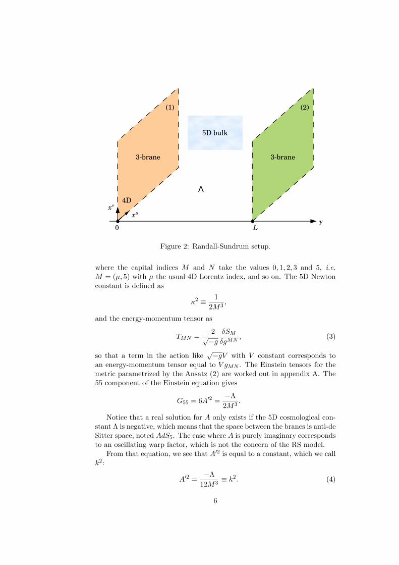
2 Setup

The Randall-Sundrum model assumes the existence of one extra dimensioncompactified on a circle whose upper and lower halves are identified (see fig.1).

Formally, this means we work in S1/Z2 orbifold, where S1 is the one-dimensional sphere (i.e. the circle) and Z2 is the multiplicative group{−1, 1}. This construction entails two fixed points, one at the origin y = 0and one at the other extremity of the circle, at y = πR ≡ L. On each ofthese boundaries stands a four-dimensional world like the one we live in. Byanalogy with membranes enclosing a volume, these worlds with 3+1 dimen-sions enclosing the 5D bulk have been called 3-branes. The picture is thentwo 3-branes, at a distance L one from another, enclosing a 5D bulk (cf. fig.2).

Taking into account the 5D cosmological constant Λ (which unlike theeffective 4D cosmological constant does not need to be vanishing or evensmall) the fundamental action is the sum of the Hilbert-Einstein action SH

and a matter part SM :

S = SH + SM =∫d4x

∫ +L

−Ldy√−g(M3R− Λ), (1)

where M is the fundamental 5D mass scale, R the 5D Ricci scalar and g thedeterminant of the metric, whose explicit form will be investigated in thenext section.

3 Warped metric

The first step is to find the metric for such a setup. Since we are lookingfor solutions to the 5D Einstein equations that might fit the real world, werequire that the metric should preserve Poincare invariance: the 4D universederived from this theory should appear flat and static. This leads to thefollowing Ansatz:

ds2 = e−2A(y)ηµνdxµdxν + dy2, (2)

where ηµν = diag(−1, 1, 1, 1) is the 4D Minkowski metric. The prefactore−2A(y), called the warp factor, is written as an exponential for convenience.Its dependence on the extra dimension coordinate y causes this metric tobe non-factorisable, which means that, unlike the metrics appearing in theusual Kaluza-Klein scenarios, it cannot be expressed as a product of the 4DMinkowski metric and a manifold of extra dimensions. To determine thefunction A(y), we have to calculate the 5D Einstein equations:

GMN = RMN −12gMNR = κ2TMN ,

5

5D bulk

y0 L

3­brane 3­brane

xµxν

(2)(1)

Λ4D

Figure 2: Randall-Sundrum setup.

where the capital indices M and N take the values 0, 1, 2, 3 and 5, i.e.M = (µ, 5) with µ the usual 4D Lorentz index, and so on. The 5D Newtonconstant is defined as

κ2 ≡ 12M3

,

and the energy-momentum tensor as

TMN =−2√−g

δSM

δgMN, (3)

so that a term in the action like√−gV with V constant corresponds to

an energy-momentum tensor equal to V gMN . The Einstein tensors for themetric parametrized by the Ansatz (2) are worked out in appendix A. The55 component of the Einstein equation gives

G55 = 6A′2 =−Λ2M3

.

Notice that a real solution for A only exists if the 5D cosmological con-stant Λ is negative, which means that the space between the branes is anti-deSitter space, noted AdS5. The case where A is purely imaginary correspondsto an oscillating warp factor, which is not the concern of the RS model.

From that equation, we see that A′2 is equal to a constant, which we callk2:

A′2 =−Λ

12M3≡ k2. (4)

6

Integrating over y gets us the expression for A:

A(y) = ±ky.

As we want a solution that respects the orbifold symmetry, i.e. invarianceunder the transformation y → −y, we choose

A(y) = k|y|.

Finally, the background metric in the Randall-Sundrum model is paramet-rized by

ds2 = e−2k|y|ηµνdxµdxν + dy2, (5)

with −L ≤ y ≤ L.Let us look now at the µν component of the 5D Einstein equations.

Appendix A gives

Gµν = (6A′2 − 3A′′)gµν .

From the solution we just found for A we see that the first derivative of Ais

A′ = sgn(y)k.

The term sgn(y) may be written as a combination of Heaviside functions as

sgn(y) = θ(y)− θ(−y),

so the second derivative is

A′′ = 2kδ(y).

This delta function arose from the kink of A at the origin y = 0 (cf. fig. 3).In the same way, the kink at y = L gives rise to another delta function, andthe complete expression for A′′ is

A′′ = 2k(δ(y)− δ(y − L)

).

Plugging those results into the expression of the Einstein tensor gives

Gµν = 6k2gµν − 6k(δ(y)− δ(y − L)

)gµν .

The first term is equal to the µν components of the energy-momentum tensormultiplied by the 5D Newton constant:

κ2Tµν =−Λ2M3

gµν = 6k2gµν .

7

A(y)

y

A’(y) A’’(y)

L0 L0L

0

Figure 3: The function A(y) and its first and second derivatives.

The second term however seems to have nothing to be matched to. Theresolution of this situation is to take into account the energy densities ofthe branes themselves, called brane tensions. This is done by adding to theaction one term for each brane, corresponding to the brane tensions λ1 andλ2:

S1 = −∫d4x

√−g1λ1 = −

∫d4xdy

√−gλ1δ(y),

S2 = −∫d4x

√−g2λ2 = −

∫d4xdy

√−gλ2δ(y − L). (6)

The terms g1 and g2 stand for the determinants of the metrics induced onthe first brane and on the second brane respectively. The induced metricsdefine distances along the branes:

ds2 = giµνdx

µdxν

= gµν(x, yi)dxµdxν ,

with i = 1, 2 and y1 = 0, y2 = L. Notice that with the metric given by (5),g1 = gδ(y) and g2 = gδ(y − L) because g55 = 1.

In order to satisfy the Einstein equations we need to impose the relation

λ1 = −λ2 = 12kM3. (7)

Moreover, by the definition of k we have

Λ = − λ21

12M3.

Those two relations are consequences of the requirement that the 4D universebe flat and static. The 4D brane sources are balanced by the 5D bulkcosmological constant in order to get a vanishing effective 4D cosmologicalconstant.

8

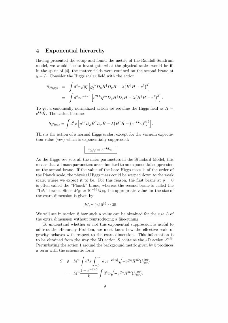
4 Exponential hierarchy

Having presented the setup and found the metric of the Randall-Sundrummodel, we would like to investigate what the physical scales would be if,in the spirit of [4], the matter fields were confined on the second brane aty = L. Consider the Higgs scalar field with the action

SHiggs =∫d4x

√g2

[gµν2 DµH

†DνH − λ(H†H − v2

)2]=

∫d4xe−4kL

[e2kLηµνDµH

†DνH − λ(H†H − v2

)2].

To get a canonically normalized action we redefine the Higgs field as H =ekLH. The action becomes

SHiggs =∫d4x

[ηµνDµH

†DνH − λ(H†H − (e−kLv)2

)2].

This is the action of a normal Higgs scalar, except for the vacuum expecta-tion value (vev) which is exponentially suppressed:

veff = e−kLv.

As the Higgs vev sets all the mass parameters in the Standard Model, thismeans that all mass parameters are submitted to an exponential suppressionon the second brane. If the value of the bare Higgs mass is of the order ofthe Planck scale, the physical Higgs mass could be warped down to the weakscale, where we expect it to be. For this reason, the first brane at y = 0is often called the “Planck” brane, whereas the second brane is called the“TeV” brane. Since MW ' 10−16MPl, the appropriate value for the size ofthe extra dimension is given by

kL ' ln1016 ' 35.

We will see in section 8 how such a value can be obtained for the size L ofthe extra dimension without reintroducing a fine-tuning.

To understand whether or not this exponential suppression is useful toaddress the Hierarchy Problem, we must know how the effective scale ofgravity behaves with respect to the extra dimension. This information isto be obtained from the way the 5D action S contains the 4D action S4D.Perturbating the action 1 around the background metric given by 5 producesa term with the schematic form

S 3 M3

∫d4x

∫ +L

−Ldye−2k|y|

√−g(0)R4D(h(0)

µν )

= M3 1− e−2kL

k

∫d4x

√−g(0)R4D(h(0)

µν ).

9

y0 L

TeV

Planckhierarchyveff = exp(­ky) v

M ~ MPl

hidden

Figure 4: The generation of an exponential hierarchy.

This term corresponds to the 4D action, so that we can read off the valueof the effective 4D Planck mass:

M2Pl = (1− e−2kL)M3/k.

We see that it weakly depends on the size of the extra dimension L, providedkL is moderately large.

Putting our two last results together, we see that the weak scale is ex-ponentially suppressed along the extra dimension, while the gravity scale ismostly independent of it (see fig.4).

In conclusion, in a theory where the values of all the bare parameters(M,Λ, λ1, v) are determined by the Planck scale, an exponential hierarchycan be naturally generated between the weak and the gravity scales. Thusthe Randall-Sundrum model provides an original solution to the HierarchyProblem.

Remarkably, the effective Planck mass remains finite even if we take thedecompactification limit L→∞. This case where there is only one brane isknown as the Randall-Sundrum II model (RS2). The fact that there couldbe an infinite extra dimension and still a 4D gravity as we experience itresults from the localization of gravity around the brane at y = 0, which wenow turn our attention to.

10

5 Graviton modes

In order to understand how gravity works in the Randall-Sundrum model,we first have to find explicit expressions for the gravitons, which correspondto small fluctuations hMN (x, y) around the background metric given by

ds2 = e−2k|y|ηµνdxµdxν + dy2.

That will be achieved by computing the solutions of the linearized Einsteinequation.

Conformally flat metric It is convenient to work with a conformally flatmetric, i.e. a metric proportional to flat space. To achieve this, we define anew extra dimension variable z related to y through

dy2 ≡ e−2k|y|dz2.

The integration of this equation produces a constant, which we set so as tohave the zero value of y corresponding to the zero value of z. The result is

k|z| = ek|y| − 1, (8)

and thus

e−2k|y| =1

(k|z|+ 1)2.

With this new coordinate, the metric is given by

ds2 =1

(k|z|+ 1)2(ηµνdx

µdxν + dz2).

To underline the fact that it is conformally flat we rewrite it in the followingway:

ds2 = e−2A(z)ηMNdxMdxN ,

where we use the notation x5 = z. The function A(z) is given by

e−2A(z) =1

(k|z|+ 1)2,

and so A(z) = ln(k|z|+ 1). For later reference, we give its first and secondderivatives:

A′(z) =sgn(z)kk|z|+ 1

, (9)

and

A′′(z) =2k(δ(z)− δ(z − Lz))

k|z|+ 1− k2

(k|z|+ 1)2, (10)

where we have used again that sgn′(z) = 2δ(z).

11

Linearized Einstein equations To keep the calculations as concise aspossible we will not compute the Einstein tensor by brute force, but ratheruse a formula about conformally related metrics (see [7] appendix D). Specif-ically, if some metric gMN is a conformal transformation of another metricgMN , for example

gMN = e−2AgMN ,

then the respective Einstein tensors are related by

GMN (gMN ) = GMN (gMN ) + (n− 2)[∇MA∇NA+ ∇M∇NA

−gMN (∇R∇RA− n− 32∇RA∇RA)

],

where n is the number of spacetime dimensions. In the present case, theperturbed metric has the form

gMN = e−2A(ηMN + hMN )

and n = 5, so the formula gives, taking into account the Christoffel symbolscontained inside the covariant derivatives:

GMN = GMN + 3[∂MA∂NA+ ∂M∂NA− ΓR

MN∂RA

−gMN (∂R∂RA− ΓR

RS∂SA− ∂RA∂

RA)]. (11)

To linear order, the Christoffel symbols are easily found:

ΓRMN =

12(∂Mh

RN + ∂Nh

RM − ∂RhMN ),

where we have used ηMN to rise the indices. It is particularly convenient inthat kind of calculations to work with a gauge in which the fluctuations donot have any extra dimension component and are transverse and traceless:

hM5 = 0,∂µhµν = 0 and ηµνhµν = hµ

µ = 0.

We verify that those 10 conditions restrict the number of degrees of freedomof the symmetric 5× 5 tensor hMN from 15 to 5, as appropriate for a spin-two 5D particle (see [8] section 2.3 and [9] section 10.6). With this gaugefixing, the second Christoffel symbol in equation (11) vanishes, whereas thefirst one reduces to −∂5hMN/2 given that it is contracted with ∂RA, whoseonly non-vanishing component is ∂5A. In addition, the expression of theEinstein tensor for fluctuations around the flat metric (see [7] eq. (4.4.5))shrinks to

GMN = −12∂R∂

RhMN .

12

The µν component of the linearized Einstein tensor in this gauge is thengiven by

Gµν = −12∂R∂

Rhµν +32h′µνA

′ − 3(ηµν + hµν)(A′′ −A′2). (12)

On the other hand, we have to compute the energy-momentum tensorfor the perturbed metric. Coming back to the expression of the action termsfor the brane tensions (6), we have to be careful about the fact that withthe conformally flat metric the determinants of the metrics induced on thebranes are now related to the determinant of the full metric by

g = gig55 = gie−2A(zi),

with i = 1, 2 and z1 = 0, z2 = Lz. The corresponding actions read

S1 = −∫d4x

√−g1λ1 = −

∫d4xdz

√−gλ1e

A(0)δ(z)

S2 = −∫d4x

√−g2λ2 = −

∫d4xdz

√−gλ2e

A(Lz)δ(z − Lz).

The µν component of the energy-momentum tensor multiplied by the 5DNewton constant is then

κ2Tµν =1

2M3

[−Λ− λ1e

Aδ(z)− λ2eAδ(z − Lz)

]gµν

=1

2M3

[−Λe−2A − λ1e

−Aδ(z)− λ2e−Aδ(z − Lz)

](ηµν + hµν).

Remembering the definition (4) of k as well as the relation (7) between thebrane-tensions and referring to the expressions (9) and (10) of the first andsecond derivatives of A allows us to rewrite it as

κ2Tµν =[6k2e−2A − 6k

(δ(z)− δ(z − Lz)

)eA](ηµν + hµν)

=[6A′2 − 3(A′′ +A′2)

](ηµν + hµν)

= (3A′2 − 3A′′)(ηµν + hµν). (13)

When we put the two sides (12) and (13) of the µν component of thelinearized Einstein equation together, the terms proportional to ηµν repro-duce the unperturbed Einstein equations, and we are left with the part dueto the perturbations:

−12∂R∂

Rhµν + 32A

′h′µν = 0.

13

Schrodinger-like equation An elegant way of solving this equation is torewrite it in the form of a Schrodinger equation.

As a start, in order to get rid of the first derivatives h′µν , we make thefollowing rescaling:

hµν → eαAhµν ,

with α a constant. A pencil and a small piece of scratch paper bring theEinstein equations to

−12∂R∂

Rhµν +(

32− α

)A′h′µν +

[(32α− 1

2α2

)A′2 − 1

2αA′′

]hµν = 0.

For the choice α = 3/2, the coefficient of h′µν vanishes and we are left with

−12∂R∂

Rhµν +[98A′2 − 3

4A′′]hµν = 0.

Performing a Kaluza-Klein decomposition,

hµν(x, z) =∞∑

n=0

hnµν(x)ψn(z),

with �hnµν ≡ ∂ρ∂

ρhnµν = m2

nhnµν , we get

−ψ′′n(z) +[

94A

′2(z)− 32A

′′(z)]ψn(z) = m2

nψn(z). (14)

That looks just like a Schrodinger equation with potential

V (z) =94A′2(z)− 3

2A′′(z)

=94

k2

(k|z|+ 1)2− 3

2

(2k(δ(z)− δ(z − Lz)

)k|z|+ 1

− k2

(k|z|+ 1)2

)

=154

k2

(k|z|+ 1)2−

3k(δ(z)− δ(z − Lz)

)k|z|+ 1

.

The shape of this potential looks like a volcano (see fig. 5).

Boundary conditions To get the boundary conditions that the solutionswill have to obey, we integrate equation (14) over small domains around theboundaries. For the boundary at z = 0 we get∫ 0+

0−dz(−ψ′′n + V ψn) =

∫ 0+

0−dzm2ψn

−ψ′n(0+) + ψ′n(0−)− 3kψn(0) = 0.

14

z0

V(z)

L­L

Figure 5: Volcano potential.

The wave-function has to be an even function under the transformationz → −z, and so its first derivative is an odd function: ψ′n(0−) = −ψ′n(0+).The boundary condition at the Planck brane is then

ψ′n(0) = −3k2ψn(0). (15)

Similarly, we get the boundary condition at the TeV brane:

ψ′n(Lz) = − 3k2(kLz + 1)

ψn(Lz). (16)

Zero-mode The zero-mode is the solution of the Schrodinger-like equationwith m0 = 0:

−ψ′′0 +[94A′2 − 3

2A′′]ψ0 = 0.

It is given by

ψ0(z) = e−32A = (k|z|+ 1)−3/2,

which satisfies the boundary conditions (15) and (16). We see that thegraviton zero-mode has a wave function that is peaked around the origin (cf.fig. 5). As we are going to see in section 7, the gravitational interactionsare predominantly mediated by the graviton zero-mode. Gravity is thuslocalized on the Planck brane, while on the TeV brane we feel only thetail of the graviton wave-function. So in the RS model the reason of the

15

z0

ψ(0)(z)

Figure 6: Localization of the graviton zero-mode around the Planck brane.

weakness of gravity is that it is localized far away from where we live — incontrast to the ADD scenario, which attributes it to the dilution of gravityin the higher-dimensional volume.

Kaluza-Klein modes Between the boundaries, the massive Kaluza-Kleinmodes have to satisfy the following equation:

ψ′′n +(m2

n −154

k2

(k|z|+ 1)2

)ψn = 0.

This is a Bessel equation of order 2 (see [10] eq. 9.1.49.), and its solutionsare linear combinations of Bessel functions of first and second kinds:

ψn = (|z|+ 1/k)1/2[anJ2

(mn(|z|+ 1/k)

)+ bnY2

(mn(|z|+ 1/k)

)], (17)

with an and bn some coefficients.To get an approximation of these wave-functions, we will use asymptotic

expressions of the Bessel functions (see [6]). We can rewrite the aboveequation as

ψn = Nn(|z|+ 1/k)1/2

[Y2

(mn(|z|+ 1/k)

)+

4k2

πm2J2

(mn(|z|+ 1/k)

)],

where Nn is a normalization constant. The coefficient in front of J2 hasbeen determined using the boundary condition (15) and the asymptoticexpressions of the Bessel functions for small arguments (mn|z| � 1):

Y2

(mn(|z|+ 1/k)

)' − 4

πm2n(|z|+ 1/k)2

− 1π

16

and

J2

(mn(|z|+ 1/k)

)' m2(|z|+ 1/k)2

8.

As k/mn � 1, the term with J2 dominates in the expression of the wavefunction. To evaluate the constant Nn, we use an approximation for largevalues of mn|z|:

√zJ2(mn|z|) ' (2/πmn)1/2cos(mn|z| − 5π/4),

which we plug in the normalization relation∫ +L

−Ldz|ψ|2 = 1.

We get ∫ +L

−LdzN2

n

32k4

π3m5n

cos2(mn|z| − 5π/4) = N2n

32k4

π3m5n

L = 1,

which implies

Nn =√π

2πm

5/2n

4k2√L.

Our approximation for the KK states wave-functions in the limit of largemn|z| is then

ψn = cos(mn|z| − 5π/4)/√L. (18)

6 Graviton spectrum

The presence of two branes induces the quantization of the masses of theKK states. To see it, let us look at the effect of the two boundary conditions(15) and (16) on the general solutions (17). The derivative of these solutionsturns out to be (cf. [10] eq. 9.1.29)

ψ′n = mn(|z|+ 1/k)1/2[anJ1

(mn(|z|+ 1/k)

)+ bnY1

(mn(|z|+ 1/k)

)]−3

2(|z|+ 1/k)−1/2

[anJ2

(mn(|z|+ 1/k)

)+ bnY2

(mn(|z|+ 1/k)

)],

so the boundary conditions become

anJ1(mn/k) + bnY1(mn/k) = 0,anJ1

(mn(Lz + 1/k)

)+ bnY1

(mn(Lz + 1/k)

)= 0.

17

This system has solutions only if its determinant vanishes, i.e. only if

J1(mn/k)Y1

(mn(Lz + 1/k)

)− J1

(mn(Lz + 1/k)

)Y1(mn/k) = 0.

Coming back to the coordinate y, which effectively represents to the distancealong the extra dimension (see equation (8)),

Lz '1kekL � 1,

we can write

J1(mn/k)Y1(mnekL/k)− J1(mne

kL/k)Y1(mn/k) = 0.

In the approximation of small masses (mn/k � 1), the Bessel functions offirst order behave like J1(mn/k) ∼ mn/k and Y1(mn/k) ∼ ln(mn/2k)mn/k(see [10] eqs. 9.4.4 and 9.4.5.), so that we can assume that −Y1(mn/k) �J1(mn/k). The requirement that the determinant vanishes reduces to

J1

(mne

kL/k)

= 0.

The masses of the KK tower are thus given by

mn = ke−kLjn,

where jn are the zeros of the Bessel function: J1(jn) = 0.As the value of k is supposed to be of order of the Planck scale and

the factor exp(−kL) at the TeV brane has been fixed to solve the HierarchyProblem, the masses of the KK states are of order TeV. Furthermore, jn+1−jn ' π, so that the splitting of the masses is also of order TeV. This impliesthe possibility to observe individual resonances of the first KK states atcolliders in the very near future [11]. Figure 6 shows an extrapolation of thecross-section for the process e+e− → µ+µ− at a linear collider, with differentvalues of the ratio k/MPl. The resonances for the first and second KK modesare well-defined and can be seen individually, in dramatic opposition to thephenomenology of the ADD scenario, which predicts only collective effects,given the smallness of the splitting between the KK modes.

7 Newtonian limit

We would like to verify that the gravitational interactions mediated by thegravitons modes that we found are in agreement with Newton’s law. For thatpurpose, we consider a minimal coupling of matter to gravity and look for thevalues of the coupling constants. The action is composed of a gravity part

18

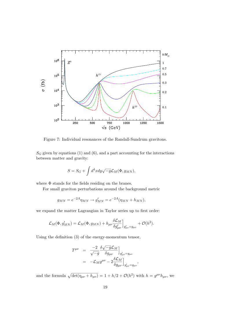
Z0

h(2)

h(1)

k/MPl

1

0.7

0.5

0.3

0.2

0.1

Figure 7: Individual resonances of the Randall-Sundrum gravitons.

SG given by equations (1) and (6), and a part accounting for the interactionsbetween matter and gravity:

S = SG +∫d4xdy

√−gLM (Φ, gMN ),

where Φ stands for the fields residing on the branes.For small graviton perturbations around the background metric

gMN = e−2AηMN → g′MN = e−2A(ηMN + hMN ),

we expand the matter Lagrangian in Taylor series up to first order:

LM (Φ, g′MN ) = LM (Φ, gMN ) + hµνδLM

δg′µν

]g′µν=gµν

+O(h2).

Using the definition (3) of the energy-momentum tensor,

Tµν =−2√−g

δ√−gLM

δgµν

]g′µν=gµν

= −LMgµν − 2

δLM

δgµν

]g′µν=gµν

,

and the formula√

det(ηµν + hµν) = 1 + h/2 + O(h2) with h = gµνhµν , we

19

can write√g′LM (φ, g′MN ) =

√g(1 + h/2)LM (φ, g′MN ) +O(h2)

=√g

[LM (Φ, gMN ) + hµν

δLM

δg′µν

]g′µν=gµν

+h

2LM (Φ, gMN )

]+O(h2)

=√g

[LM (Φ, gMN )− 1

2hµνT

µν

]+O(h2).

On the other side, when we expand SG up to the second order in theperturbations, we get the following terms: one part independent of hµν thatvanishes because of the requirement of the vanishing of the effective cosmo-logical constant; one linear part, which is the action leading to the linearequations of motion, so that it vanishes on shell; and one quadratic part,which corresponds the usual Pauli-Fierz Lagrangian LPF . Remembering thesolution we found for the KK modes after a rescaling by exp(3A/2) and aKK decomposition drives us to

LM (Φ, g′MN ) = LM (Φ, gMN ) +M3∑

n

LPF (hnµν(x))

−∑

n

e32Aψ(n)(z)

2hn

µν(x)Tµν

In order to get a canonically normalized Pauli-Fierz Lagrangian, we proceedto a field redefinition:

hnµν(x) →

1√M3

hnµν(x),

and we finally obtain

LM (φ, g) = LM (Φ, η) +∑

n

LPF (hnµν(x))−

∑n

e32Aψn(z)

2√M3

hnµν(x)T

µν ,

from which we can read the expression of the gravity-matter coupling con-stants:

an =e

32Aψn(z)

2√M3

.

We can now compute the gravitational potential between two particleswith unit masses on the TeV brane at z = Lz, i.e. the static potentialgenerated by the exchange of the zero-mode and the massive KK states.Like in the case of a Yukawa interaction (see [12] eq. (4.127)), it is given by

V (r) = −∞∑

n=0

a2n

4πe−mnr

r.

20

The contribution of the zero-mode ψ0(z) = exp(−3A/2) to the gravita-tional interaction is

V0(r) = − 116πM3

1r

= −GN

r,

with GN the Newton constant. This reproduces the 4D gravity.With the help of the approximation (18) for the KK states wave-fun-

ctions, the non-relativistic gravitational potential mediated by the nth mas-sive graviton on the TeV brane reads

Vn(r) = − k3L2

16πM3cos2(mnLz − 5π/4)

e−mnr

r

= −GN

rk3L2cos2(mnLz − 5π/4)e−mnr.

These contributions to the gravitational potential are exponentially sup-pressed, and thus may be neglected down to distances of order of the fermi,r . 10−13 cm. The actual experimental tests of gravity having only probeddown to the millimeter scale, there is no perspective of detecting such smallcorrections any time soon.

In conclusion, gravity in the RS model corresponds effectively to 4Dgravity as we experience it.

8 Radius stabilization

Until now we have treated the length, or equivalently the radius, of theextra dimension as a parameter, and we felt free to set it to the appropriatevalue to solve the Hierarchy Problem (see section 4). However, such a degreeof freedom would imply the existence in the effective theory of a masslessscalar field, corresponding to the fluctuations of the radius along the extradimension: the radion. This massless radion would cause a fifth force inviolation to the equivalence principle. Therefore, to preserve the viabilityof the Randall-Sundrum model, the radion has to obtain a mass, i.e. to bestabilized.

A way to do it is the Goldberger-Wise mechanism [13]. The idea is tointroduce a massive scalar field φ in the bulk with a potential V (φ) and addsome potentials V1(φ) and V2(φ) on the two branes at the boundaries. Thecorresponding action reads

S =∫d4xdy

√−g[M3R+

12∂Mφ∂

Mφ− V (φ)

−V1(φ)δ(y)− V2(φ)δ(y − L)].

21

The requirement of Poincare invariance imposes to choose the metricgiven by

ds2 = e−2A(y)ηµνdxµdxν + dy2,

and to restrict the dependence of the scalar field to the extra dimension:

φ(x, y) = φ(y).

To find φ(y), the scalar field and the Einstein equations should be solvedsimultaneously. The scalar equation is

1√−g

∂M√−ggMN∂Nφ = −∂Vtot

∂φ,

with Vtot = −V − V1δ(y) − V2δ(y − L). Only the 55 component gives anon-vanishing result:

φ′′ − 4A′φ′ =∂V

∂φ+∂V1

∂φδ(y) +

∂V2

∂φδ(y − L).

Referring to the expression of the Einstein tensors found in appendix A,the 55 and µν components of the Einstein equations GMN = κ2TMN are

A′2 =κ2

12φ′2 − κ2

6V (φ), (19)

and

2A′2 −A′′ =κ2

6φ′2 − κ2

3(V + V1δ(y) + V2δ(y − L)).

We can simplify the second result by using the first one to eliminate φ′:

A′′ =κ2

3(V1δ(y) + V2δ(y − L)).

To obtain the boundary conditions, we integrate those results on verysmall domains around the positions y1 = 0 and y2 = L. The kinks of φ andA at those positions will result in jumps in the derivatives:

φ′]y+

i

y−i

=∂Vi

∂φ,

and

A′]y+

i

y−i

=κ2

3Vi.

Together with the scalar and Einstein equations these equations form thegravity-scalar system. It is quite hard to solve generally, so we will restrainour study to a special case.

22

Suppose that V has the special form

V (φ) =18

(∂W (φ)∂φ

)2

− κ2

6W 2(φ),

for some function W (φ), called “superpotential”. As equation (19) can bewritten as

V (φ) =12φ′2 − 6

κ2A′2,

we conclude that

φ′ =12∂W

∂φand A′ =

κ2

6W (φ).

We want the bulk potential to include a cosmological constant term(independent of φ) and a mass term (quadratic in φ), so we choose forexample

W =6kκ2− uφ2,

with u a parameter. From that we have

φ′ =12∂W

∂φ= −uφ,

whose solution is easily found:

φ(y) = φP e−uy.

On the TeV brane we get

φT = φP e−uL,

which can be inverted to

L = ln(φP /φT )/u.

The value of the radius is thus determined by the equation of motion. Tosolve the Hierarchy Problem, we need kL ' 35, which only implies a modesttuning of order O(50) on the input parameters. Thus the solution to theHierarchy Problem provided by the Randall-Sundrum model does not arise –like in the case of large extra dimensions – at the cost of introducing anotherfine-tuning.

23

Acknowledgments

One of us (MG) would like to express his gratitude to Antonios Papazogloufor the patient guidance of his first hesitating steps in general relativity:cheers!

References

[1] T. Kaluza, Sitzungsber. Preuss. Akad. Wiss. Berlin (Math. Phys.) K1,966 (1921); O. Klein, Z. Phys. 37, 895 (1926).

[2] J. Polchinski, String Theory, Cambridge, Vol. I, chap. 8: Toroidal com-pactification and T -duality (1995).

[3] N. Arkani-Hamed, S. Dimopoulos and G.R. Dvali, Phys. Rev. D59,086004 (1999) hep-ph/9807344.

[4] V. A. Rubakov and M. E. Shaposhnikov, Do We Live inside a DomainWall?, Phys. Lett. B125, 136 (1983).

[5] L. Randall and R. Sundrum, A Large Mass Hierarchy from a SmallExtra Dimension, Phys. Rev. Lett. 83, 3370 (1999).

[6] L. Randall and R. Sundrum, An Alternative to Compactification, Phys.Rev. Lett. 83, 4690 (1999).

[7] R. M. Wald, General Relativity, The University of Chicago Press, 1984.

[8] C. Csaki, TASI Lectures on Extra Dimensions and Branes (2002) hep-ph/0404096.

[9] B. Zwiebach, A First Course in String Theory, Cambridge UniversityPress, 2005.

[10] M. Abramowitz and I. A. Stegun, Handbook of Mathematical Functions,Dover Publications, 1972.

[11] H. Davoudiasl, J. L. Hewett and T. G. Rizzo, Phys. Rev. Lett. 84, 2080(2000).

[12] M. E. Peskin and D. V. Schroeder, An Introduction to Quantum FieldTheory, Addison-Wesley Publishing Company, 1995.

[13] W. D. Goldberger and M. B. Wise, Modulus Stabilization with BulkFields, Phys. Rev. Lett. 83, 4922 (1999) hep-ph/9907447.

24

A Einstein tensor

We want to calculate the Einstein tensor for the metric

ds2 = e−2A(y)ηµνdxµdxν + dy2

= gMN (y)dxMdxN ,

with

gMN (y) = e−2A(y)ηµν + δ5Mδ5N .

The inverse metric is

gMN (y) = e2A(y)ηµν + δM5 δN

5 .

Christoffel symbols

ΓPMN =

12gPR(∂MgNR + ∂NgRM − ∂RgMN ).

As gMN is a function of the extra dimension only, and this only in its µνcomponents, we have

∂LgMN = ∂5gMN = ∂5gµν .

That implies that only two types of Christoffel symbols are non-vanishing:

Γ5µν =

12g5R(−∂Rgµν)

=12g55(−∂5gµν)

= A′e−2Aηµν ,

and

Γνµ5 =

12gνR(∂5gRµ)

=12e2Aηνρ(−2A′e−2Aηρµ)

= −A′δνµ.

Ricci tensor

RMN = ∂P ΓPMN − ∂NΓP

MP + ΓPPQΓQ

MN − ΓPNQΓQ

MP .

Rµν = ∂5Γ5µν + Γσ

σ5Γ5µν − Γσ

ν5Γ5µσ − Γ5

νσΓσµ5

= (A′′ − 2A′2)e−2Aηµν − 4A′2e−2Aηµν

+A′2e−2Aηµν +A′2e−2Aηµν

= (A′′ − 4A′2)gµν .

25

Rµ5 = 0.

R55 = −∂5Γσ5σ − Γσ

5ρΓρ5σ

= 4A′′ − 4A′2.

Ricci scalar

R = gMNRMN

= gµνRµν + g55R55

= 4(A′′ − 4A′2) + 4A′′ − 4A′2

= 8A′′ − 20A′2.

Einstein tensor

Gµν = Rµν −12gµνR

= (6A′2 − 3A′′)gµν .

G55 = R55 −12g55R

= 6A′2.

26