The random walk Metropolis: linking theory and

practice through a case study.

Chris Sherlock1,3, Paul Fearnhead1, and Gareth O. Roberts2

1. Department of Mathematics and Statistics, Lancaster University, Lancaster, LA1 4YF,

UK

2. Department of Statistics, University of Warwick, Coventry, CV4 7AL, UK.

3. Correspondence should be addressed to Chris Sherlock.

(e-mail: c.sherlock@lancs.ac.uk).

Summary: The random walk Metropolis (RWM) is one of the most common Markov Chain

Monte Carlo algorithms in practical use today. Its theoretical properties have been exten-

sively explored for certain classes of target, and a number of results with important practical

implications have been derived. This article draws together a selection of new and existing

key results and concepts and describes their implications. The impact of each new idea on

algorithm efficiency is demonstrated for the practical example of the Markov modulated Pois-

son process (MMPP). A reparameterisation of the MMPP which leads to a highly efficient

RWM within Gibbs algorithm in certain circumstances is also presented.

Keywords: random walk Metropolis, Metropolis-Hastings, MCMC, adaptive MCMC, MMPP

1

1 Introduction

Markov chain Monte Carlo (MCMC) algorithms provide a framework for sampling from

a target random variable with a potentially complicated probability distribution π(·) by

generating a Markov chain X(1),X(2), . . . with stationary distribution π(·). The single most

widely used sub-class of MCMC algorithms is based around the random walk Metropolis

(RWM).

Theoretical properties of RWM algorithms for certain special classes of target have been in-

vestigated extensively. Reviews of RWM theory have, for example, dealt with optimal scaling

and posterior shape (Roberts and Rosenthal, 2001), and convergence (Roberts, 2003). This

article does not set out to be a comprehensive review of all theoretical results pertinent to

the RWM. Instead the article reviews and develops specific aspects of the theory of RWM

efficiency in order to tackle an important and difficult problem: inference for the Markov

modulated Poisson process (MMPP). It includes sections on RWM within Gibbs, hybrid

algorithms, and adaptive MCMC, as well as optimal scaling, optimal shaping, and conver-

gence. A strong emphasis is placed on developing an intuitive understanding of the processes

behind the theoretical results, and then on using these ideas to improve the implementation.

All of the RWM algorithms described in this article are tested against data sets arising from

MMPPs. Realised changes in efficiency are then compared with theoretical predictions.

Observed event times of an MMPP arise from a Poisson process whose intensity varies

with the state of an unobserved continuous time Markov chain. The MMPP has been

used to model a wide variety of clustered point processes, for example requests for web

pages from users of the World Wide Web (Scott and Smyth, 2003), arrivals of photons from

single molecule fluorescence experiments (Burzykowski et al., 2003; Kou et al., 2005), and

occurences of a rare DNA motif along a genome (Fearnhead and Sherlock, 2006).

In common with mixture models and other hidden Markov models, inference for the MMPP

2

is greatly complicated by a lack of knowledge of the hidden data. The likelihood function

often possesses many minor modes since the data might be approximately described by a

hidden process with fewer states. For this same reason the likelihood often does not appoach

zero as certain combinations of parameters approach zero and/or infinity and so improper

priors lead to improper posteriors (e.g. Sherlock, 2005). Further, as with many hidden

data models the likelihood is invariant under permutation of the states, and this “labelling”

problem leads to posteriors with several equal modes.

This article focusses on generic concepts and techniques for improving the efficiency of RWM

algorithms whatever the statistical model. The MMPP provides a non-trivial testing ground

for them. All of the RWM algorithms described in this article are tested against two sim-

ulated MMPP data sets with very different characteristics. This allows us to demonstrate

the influence on performance of posterior attributes such as shape and orientation near the

mode and lightness or heaviness of tails.

Section 2 introduces RWM algorithms and then describes theoretical and practical measures

of algorithm efficiency. Next the two main theoretical approaches to determining efficiency

are decribed, and the section ends with a brief overview of the MMPP and a description

of the data analysed in this article. Section 3 introduces a series of concepts which allow

potential improvements in the efficiency of a RWM algorithm. The intuition behind each

concept is described, followed by theoretical justification and then details of one or more

RWM algorithms motivated by the theory. Actual results are described and compared with

theoretical predictions in Section 4, and the article is summarised in Section 5.

3

2 Background

In this section we introduce the background material on which the remainder of this article

draws. We describe the random walk Metropolis algorithm and a variation, the random

walk Metropolis-within-Gibbs. Both practical issues and theoretical approaches to algorithm

efficiency are then discussed. We conclude with an introduction to the Markov modulated

Poisson process and to the data sets used later in the article.

2.1 Random walk Metropolis algorithms

The random walk Metropolis (RWM) updating scheme was first applied in Metropolis

et al. (1953) and proceeds as follows. Given a current value of the d-dimensional Markov

chain, X, a new value X∗ is obtained by proposing a jump Y∗ := X∗ − X from the pre-

specified Lebesgue density

r (y∗;λ) :=1

λdr

(

y∗

λ

)

, (1)

with r(y) = r(−y) for all y. Here λ > 0 governs the overall size of the proposed jump and

(see Section 3.1) plays a crucial role in determining the efficiency of any algorithm. The

proposal is then accepted or rejected according to acceptance probability

α(x,y∗) = min

(

1,π(x + y∗)

π(x)

)

. (2)

If the proposed value is accepted it becomes the next current value (X′ ← X+Y∗), otherwise

the current value is left unchanged (X′ ← X).

An intuitive interpretation of the above formula is that “uphill” proposals (proposals which

take the chain closer to a local mode) are always accepted, whereas “downhill” proposals

are accepted with probability exactly equal to the relative “heights” of the posterior at the

proposed and current values. It is precisely this rejection of some “downhill” proposals which

acts to keep the Markov chain in the main posterior mass most of the time.

4

More formally, denote by P (x, ·) the transition kernel of the chain, which represents the com-

bined process of proposal and acceptance/rejection leading from one element of the chain (x)

to the next. The acceptance probability (2) is chosen so that the chain is reversible at equi-

librium with stationary distribution π(·). Reversibility (that π(x)P (x,x′) = π(x′)P (x′,x))

is an important property precisely because it is so easy to construct reversible chains which

have a pre-specified stationary distribution. It is also possible to prove a slightly stronger cen-

tral limit theorem for reversible (as opposed to non-reversible) geometrically ergodic chains

(e.g. Section 2.2.1).

We now describe a generalisation of the RWM which acts on a target whose components

have been split into k sub-blocks. In general we write X = (X1, . . . ,Xk), where Xi is the

ith sub-block of components of the current element of the chain. Starting from value X, a

single iteration of this algorithm cycles through all of the sub-blocks updating each in turn.

It will therefore be convenient to define the shorthand

x(B)i := x′

1, . . . ,x′i−1,xi,xi+1, . . . ,xk

x(B)∗i := x′

1, . . . ,x′i−1,xi + y∗

i ,xi+1, . . . ,xk ,

where x′j is the updated value of the jth sub-block. For the ith sub-block a jump Y ∗

i is proposed

from symmetric density ri(y;λi) and accepted or rejected according to acceptance probability

π(

x(B)∗i

)

/π(

x(B)i

)

. Since this algorithm is in fact a generalisation of both the RWM and of

the Gibbs sampler (for a description of the Gibbs sampler see for example Gamerman and

Lopes, 2006) we follow for example Neal and Roberts (2006) and call this the random walk

Metropolis-within-Gibbs or RWM-within-Gibbs. The most commonly used random walk

Metropolis within Gibbs algorithm, and also the simplest, is that employed in this article:

here all blocks have dimension 1 so that each component of the parameter vector is updated

in turn.

As mentioned earlier in this section, the RWM is reversible; but even though each stage of

the RWM-within-Gibbs is reversible, the algorithm as a whole is not. Reversible variations

5

include the random scan RWM-within-Gibbs, wherein at each iteration a single component

is chosen at random and updated conditional on all the other components.

Convergence of the Markov chain to its stationary distribution can be guaranteed for all of

the above algorithms under quite general circumstances (e.g. Gilks et al., 1996).

2.2 Algorithm efficiency

Consecutive draws of an MCMC Markov chain are correlated and the sequence of marginal

distributions converges to π(·). Two main (and related) issues arise with regard to the

efficiency of MCMC algorithms: convergence and mixing.

2.2.1 Convergence

In this article we will be concerned with practical determination of a point at which a chain

has converged. The method we employ is simple heuristic examination of the trace plots for

the different components of the chain. Note that since the state space is multi-dimensional it

is not sufficient to simply examine a single component. Alternative techniques are discussed

in Chapter 7 of Gilks et al. (1996).

Theoretical criteria for ensuring convergence (ergodicity) of MCMC Markov chains are ex-

amined in detail in Chapters 3 and 4 of Gilks et al. (1996) and references therein, and will

not be discussed here. We do however wish to highlight the concepts of geometric and poly-

nomial ergodicity. A Markov chain is with transition kernel P is geometrically ergodic

with stationary distribution π(·) if

||P n(x, ·)− π(·)||1 ≤ M(x) rn (3)

for some positive r < 1 and M(·) ≥ 0; if M(·) is bounded above then the chain is uniformly

6

ergodic. Here ||F (·)−G(·)||1 denotes the total variational distance between measures F (·)

and G(·) (see for example Meyn and Tweedie, 1993), and P n is the n-step transition kernel.

Efficiency of a geometrically ergodic algorithm is measured by the geometric rate of conver-

gence, r, which over a large number of iterations is well approximated by the second largest

eigenvalue of the transition kernel (the largest eigenvalue being 1, and corresponding to the

stationary distribution π(·)). Geometric ergodicity is usually a purely qualitative property

since in general the constants M(x) and r are not known. Crucially for practical MCMC

however any geometrically ergodic reversible Markov chain satisfies a central limit theorem

for all functions with finite second moment with respect to π(·). Thus there is a σ2f <∞ such

that

n1/2(

fn − Eπ [f(X)])

⇒ N(0, σ2f) (4)

where ⇒ denotes convergence in distribution. The central limit theorem (4) guarantees not

only convergence of the Monte Carlo estimate (5) but also supplies its standard error, which

decreases as n−1/2.

When the second largest eigenvalue is also 1 a Markov chain is termed polynomially er-

godic if

||P n(x, ·)− π(·)||1 ≤M(x) n−r

Clearly polynomial ergodicity is a weaker condition than geometric ergodicity. Central limit

theorems for polynomially ergodic MCMC are much more delicate; see Jarner and Roberts

(2002) for details.

In this article a chain is referred to as having “reached stationarity” or “converged” when

the distribution from which an element is sampled is as close to the stationary distribution

as to make no practical difference to any Monte-Carlo estimates.

An estimate of the expectation of a given function f(X), which is more accurate than a

naive Monte Carlo average over all the elements of the chain, is likely to be obtained by

discarding the portion of the chain X0, . . . ,Xm up until the point at which it was deemed to

7

have reached stationarity; iterations 1, . . .m are commonly termed “burn in”. Using only the

remaining elements Xm+1, . . . ,Xm+n (with m+n = N) our Monte Carlo estimator becomes

fn :=1

n

m+n∑

m+1

f(Xi) (5)

Convergence and burn in are not discussed any further here, and for the rest of this section

the chain is assumed to have started at stationarity and continued for n further iterations.

2.2.2 Practical measures of mixing efficiency

For a stationary chain, X0 is sampled from π(·), and so for all k > 0 and i ≥ 0

Cov [f(Xk), f(Xk+i)] = Cov [f(X0), f(Xi)]

This is the autocorrelation at lag i. Therefore at stationarity, from the definition in (4),

σ2f := lim

n→∞nVar

[

fn

]

= Var [f(X0)] + 2

∞∑

i=1

Cov [f(X0), f(Xi)]

provided the sum exists (e.g. Geyer, 1992). If elements of the stationary chain were inde-

pendent then σ2f would simply be Var [f(X0)] and so a measure of the inefficiency of the

Monte-Carlo estimate fn relative to the perfect i.i.d. sample is

σ2f

Var [f(X0)]= 1 + 2

∞∑

i=1

Corr [f(X0), f(Xi)] (6)

This is the integrated autocorrelation time (ACT) and represents the effective number of

dependent samples that is equivalent to a single independent sample. Alternatively n∗ =

n/ACT may be regarded as the effective equivalent sample size if the elements of the chain

had been independent.

To estimate the ACT in practice one might examine the chain from the point at which it is

deemed to have converged and estimate the lag-i autocorrelation Corr [f(X0), f(Xi)] by

γi =1

n− i

n−i∑

j=1

(

f(Xj)− fn)(

f(Xj+i)− fn)

(7)

8

Naively, substituting these into (6) gives an estimate of the ACT. However contributions

from all terms with very low theoretical autocorrelation in a real run are effectively random

noise, and the sum of such terms can dominate the deterministic effect in which we are

interested (e.g. Geyer, 1992). For this article we employ the simple solution suggested in

Carlin and Louis (2009): the sum (6) is truncated from the first lag, l, for which the estimated

autocorrelation drops below 0.05 . This gives the (slightly biassed) estimator

ACTest := 1 + 2l−1∑

i=1

γi. (8)

Given the potential for relatively large variance in estimates of integrated ACT howsoever

they might be obtained (e.g. Sokal, 1997), this simple estimator should be adequate for

comparing the relative efficiencies of the different algorithms in this article. Geyer (1992)

provides a number of more complex window estimators and provides references for regularity

conditions under which they are consistent.

A given run will have a different ACT associated with each parameter. An alternative

efficiency measure, which is aggregated over all parameters is provided by the Mean Square

Euclidean Jump Distance (MSEJD)

S2Euc :=

1

n− 1

n−1∑

i=1

∣

∣

∣

∣x(i+1) − x(i)∣

∣

∣

∣

2

2.

The expectation of this quantity at stationarity is referred to as the Expected Square Eu-

clidean Jump Distance (ESEJD). Consider a single component of the target with variance

σ2i := Var [Xi] = Var [X ′

i], and note that E [X ′i −Xi] = 0, so

E[

(X ′i −Xi)

2]

= Var [X ′i −Xi] = 2σ2

i (1− Corr [Xi, X′i])

Thus when the chain is stationary and the posterior variance is finite, maximising the ESEJD

is equivalent to minimising a weighted sum of the lag-1 autocorrelations.

If the target has finite second moments and is roughly elliptical in shape with (known)

covariance matrix Σ then an alternative measure of efficiency is the Mean Square Jump

9

0 200 400 600 800

−3

−2

−1

01

23

(a) Chain: lambda=0.24

0 10 20 30 40

0.0

0.2

0.4

0.6

0.8

1.0

Lag

AC

F

(d) ACF: lambda=0.24

0 200 400 600 800

−3

−2

−1

01

23

(b) Chain: lambda=2.4

0 10 20 30 40

0.0

0.2

0.4

0.6

0.8

1.0

Lag

AC

F

(e) ACF: lambda=2.4

0 200 400 600 800

−3

−2

−1

01

23

(c) Chain: lambda=24

0 10 20 30 40

0.0

0.2

0.4

0.6

0.8

1.0

Lag

AC

F

(f) ACF: lambda=24

xxx

Figure 1: Trace plots ((a), (b), and (c)) and corresponding autocorrelation plots ((d), (e), and

(f)), for exploration of a standard Gaussian initialised from x = 0 and using the random walk

Metropolis algorithm with Gaussian proposal for 1000 iterations. Proposal scale parameters for

the three scenarios are respectively (a) & (d) 0.24, (b) & (e) 2.4, and (c) & (f) 24.

Distance (MSJD)

S2d :=

1

n− 1

n−1∑

i=1

(

x(i+1) − x(i))t

Σ−1(

x(i+1) − x(i))

,

which is proportional to the unweighted sum of the lag-1 autocorrelations over the principal

components of the ellipse. The theoretical expectation of the MSJD at stationarity is known

as the expected squared jump distance (ESJD).

Figure 1 shows trace plots for three different Markov chains. Estimates of the autocorrelation

from lag-0 to lag-40 for each Markov chain appear alongside the corresponding traceplot.

The simple window estimator for integrated ACT provides estimates of respectively 39.7,

5.5, and 35.3. The MSEJDs are respectively 0.027, 0.349, and 0.063, and are equal to the

MSJDs since the stationary distribution has a variance of 1.

10

2.2.3 Assessing accuracy

An MCMC algorithm might efficiently explore an unimportant part of the parameter space

and never find the main posterior mass. ACT’s will be low therefore, but the resulting

posterior estimate will be wildly innaccurate. In most practical examples it is not possible

to determine the accuracy of the posterior estimate, though consistency between several

independent runs or between different portions of the same run can be tested.

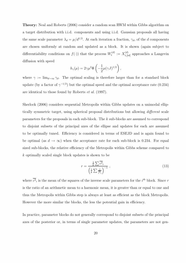
For the purposes of this article it was important to have a relatively accurate estimate of

the posterior, not determined by a RWM algorithm. Fearnhead and Sherlock (2006) detail

a Gibbs sampler for the MMPP; this Gibbs sampler was run for 100 000 iterations on each

of the data sets analysed in this article. A “burn-in” of 1000 iterations was allowed for, and

a posterior estimate from the last 99 000 iterations was used as a reference for comparison

with posterior estimates from RWM runs of 10 000 iterations (after burn in).

2.2.4 Theoretical approaches for algorithm efficiency

To date, theoretical results on the efficiency of RWM algorithms have been obtained through

two very different approaches. We wish to quote, explain, and apply theory from both and

so we give a heuristic description of each and define associated notation. Both approaches

link some measure of efficiency to the expected acceptance rate - the expected proportion of

proposals accepted at stationarity.

The first approach was pioneered in Roberts et al. (1997) for targets with independent

identically distributed components and then generalised in Roberts and Rosenthal (2001) to

targets of the form

π(x) =

d∏

1

Ci f(Cixi).

The inverse scale parameters, Ci, are assumed to be drawn from some distribution with a

11

given (finite) mean and variance. A single component of the d dimensional chain (without

loss of generality the first) is then examined; at iteration i of the algorithm it is denoted

X(d)1,i . A scaleless, speeded up, continuous time process which mimics the first component of

the chain is defined as

W(d)t := C1X

(d)1,[td],

where [u] denotes the nearest integer less than or equal to u. Finally, proposed jumps are

assumed to be Gaussian

Y(d) ∼ N(

0, λ2dI)

.

Subject to conditions on the first two deriviatives of f(·), Roberts and Rosenthal (2001)

show that if E [Ci] = 1 and E [C2i ] = b, and provided λd = µ/d1/2 for some fixed µ (the

scale parameter but “rescaled” according to dimension) then as d→ ∞, W(d)t approaches

a Langevin diffusion process with speed

h(µ) =C2

1µ2

bαd where αd := 2Φ

(

−1

2µJ1/2

)

. (9)

Here Φ(x) is the cumulative distribution function of a standard Gaussian, J := E[

((log f)′)2]

is a measure of the roughness of the target, and αd corresponds to the acceptance rate.

Bedard (2007) proves a similar result for a triangular sequence of inverse scale parameters

ci,d, which are assumed to be known. A necessary and sufficient condition equivalent to (11)

below is attached to this result. In effect this requires the scale over which the smallest

component varies to be “not too much smaller” than the scales of the other components.

The second technique (e.g. Sherlock and Roberts, 2009) uses expected square jump distance

(ESJD) as a measure of efficiency. Exact analytical forms for ESJD (denoted S2d) and

expected acceptance rate are derived for any unimodal elliptically symmetric target and any

proposal density. Many standard sequences of d-dimensional targets (d = 1, 2, . . . ), such as

the Gaussian, satisfy the condition that as d→∞ the probability mass becomes concentrated

in a spherical shell which itself becomes infinitesimally thin relative to its radius. Thus the

12

random walk on a rescaling of the target is, in the limit, effectively confined to the surface

of this shell. Sherlock and Roberts (2009) consider a sequence of targets which satisfies such

a “shell” condition, and a sequence of proposals which satisfies a slightly stronger condition.

Specifically it is required that there exist sequences of positive real numbers, {k(d)x } and

{k(d)y }, such that

∣

∣

∣

∣X(d)∣

∣

∣

∣

k(d)x

p−→ 1 and

∣

∣

∣

∣Y(d)∣

∣

∣

∣

λd k(d)y

m.s.−→ 1.

For such combinations of target and proposal, as d→∞

d

k(d)x

2S2d(µ)→ µ2 αd with αd(µ) := 2Φ

(

−1

2µ

)

. (10)

Here αd is the limiting expected acceptance rate, and µ := d1/2λdk(d)y /k

(d)x . For target and

proposal distributions with independent components, such as are used in the diffusion results,

k(d)x = k

(d)y = d1/2, and hence (consistently) µ = d1/2λd.

It is also required that the elliptical target not be too eccentric. Specifically, for a sequence of

target densities πd(x) := fd

(

∑di=1 c

2i,dx

2i

)

(for some appropriate sequence of functions {fd})

maxi c2i,d

∑di=1 c

2i,d

→ 0 as d→∞. (11)

Theoretical results from the two techniques are remarkably similar and as will be seen, lead

to identical strategies for optimising algorithm efficiency. It is worth noting however that

results from the first approach apply only to targets with independent components and

results from the second only to targets which are unimodal and elliptically symmetric. That

they lead to identical strategies indicates a certain potential robustness of these strategies

to the form of the target. This potential, as we shall see, is born out in practice.

13

0 2 4 6 8 10

0 2 4 6 8 10

222

111

state

state

Figure 2: Two 2-state continuous time Markov chains simulated for 10 seconds from generator Q

with q12 = q21 = 1; the rug plots show events from an MMPP simulated from these chains, with

intensity vectors ψ = [10, 30] (upper graph) and ψ = [10, 17] (lower graph).

2.3 The Markov Modulated Poisson Process

Let Xt be a continuous time Markov chain on discrete state space {1, . . . , d} and let ψ :=

[ψ1, . . . , ψd] be a d-dimensional vector of (non-negative) intensities. The linked but stochas-

tically independent Poisson process Yt whose intensity is ψXt is a Markov modulated Poisson

process - it is a Poisson process whose intensity is modulated by a continuous time Markov

chain.

The idea is best illustrated through two examples, which also serve to introduce the notation

and data sets that will be used throughout this article. Consider a two-dimensional Markov

chain Xt with generator Q with q12 = q21 = 1.

Figure 2 shows realisations from two such chains over a period of 10 seconds. Now consider

a Poisson process Yt which has intensity 10 when Xt is in state 1 and intensity 30 when

Xt is in state 2. This is an MMPP with event intensity vector ψ = [10, 30]. A realisation

(obtained via the realisation of Xt) is shown as a rug plot underneath the chain in the upper

graph. The lower graph shows a realisation from an MMPP with event intensities [10, 17].

14

It can be shown (e.g. Fearnhead and Sherlock, 2006) that the likelihood for data from an

MMPP which starts from a distribution ν over its states is

L(Q,Ψ, t) = ν ′e(Q−Ψ)t1Ψ . . . e(Q−Ψ)tnΨe(Q−Ψ)tn+11. (12)

Here Ψ := diag(ψ), 1 is a vector of 1’s, n is the number of observed events, t1 is the time

from the start of the observation window until the first event, tn+1 is the time from the last

event until the end of observation window, and ti (2 ≤ i ≤ n) is the time between the i− 1th

and ith events. In the absence of further information, the initial distribution ν is often taken

to be the stationary distribution of the underlying Markov chain.

The likelihood of an MMPP is invariant to a relabelling of the states. Hence if the prior is

similarly invariant then so too is the posterior: if the posterior for a two dimensional MMPP

has a mode at (ψ1, ψ2, q12, q21) then it has an identical mode at (ψ2, ψ1, q21, q12). In this

article our overriding interest is in the efficiency of the MCMC algorithms rather than the

exact meaning of the parameters and so we choose the simplest solution to this identifiablity

problem: the state with the lower Poisson intensity ψ is always referred to as State 1.

2.3.1 MMPP data in this article

The two data sets of event times used in this article arose from two independent MMPP’s

simulated over an observation window of 100 seconds. Both underlying Markov chains have

q12 = q21 = 1; data set D1 has event intensity vector ψ = [10, 30] whereas data set D2 has

ψ = [10, 17], so that the overall intensity of events in D2 is lower than in D1. As mentioned

in Section 2.2.3, a posterior sample from a long run of the Gibbs sampler of Fearnhead and

Sherlock (2006) was used to approximate the true posterior. Figure 3 shows estimates of the

marginal posterior distribution for (ψ1, ψ2) and for (ψ1, q12) for D1 (top) and D2 (bottom).

Because the difference in intensity between the states is so much larger in D1 than in D2 it is

easier with D1 than D2 to distinguish the state of the underlying Markov chain, and thus the

15

8 9 10 11 12

2728

2930

3132

8 9 10 11 12

0.6

0.8

1.0

1.2

1.4

1.6

6 7 8 9 10 11 12 13

1415

1617

1819

6 7 8 9 10 11 12 13

0.0

0.5

1.0

1.5

ψ1ψ1

ψ1ψ1

ψ2

ψ2

q12

q12

Figure 3: Estimated marginal posteriors for ψ1 and ψ2 and for ψ1 and q12 from long runs of the

Gibbs sampler for data sets D1 (top) and D2 (bottom).

values of the Markov and Poisson parameters. Further, in the limit of the underlying chain

being known precisely, for example as ψ2 → ∞ with ψ1 finite, and provided the priors are

independent, the posteriors for the Poisson intensity parameters ψ1 and ψ2 are completely

independent of each other and of the Markov parameters q12 and q21. Dependence between

the Markov parameters is also small, being O(1/T ) (e.g. Fearnhead and Sherlock, 2006).

In Section 4, differences between D1 and D2 will be related directly to observed differences

in efficiency of the various RWM algorithms between the two data sets.

3 Implementations of the RWM: theory and practice

This section describes several theoretical results for the RWM or for MCMC in general.

Intuitive explanation of the principle behind each result is emphasised and the manner in

16

which it informs the RWM implementation is made clear. Each algorithm was run three

times on each of the two data sets.

3.1 Optimal scaling of the RWM

Intuition: Consider the behaviour of the RWM as a function of the overall scale parameter

of the proposed jump, λ, in (1). If most proposed jumps are small compared with some

measure of the scale of variability of the target distribution then, although these jumps will

often be accepted, the chain will move slowly and exploration of the target distribution

will be relatively inefficient. If the jumps proposed are relatively large compared with the

target distribution’s scale, then many will not be accepted, the chain will rarely move and

will again explore the target distribution inefficiently. This suggests that given a particular

target and form for the jump proposal distribution, there may exist a finite scale parameter

for the proposal with which the algorithm will explore the target as efficiently as possible.

These ideas are clearly demonstrated in Figure 1 which shows traceplots for a one dimen-

sional Gaussian target explored using a Gaussian proposal with scale parameter an order of

magnitude smaller (a) and larger (c) than is optimal, and (b) with a close to optimal scale

parameter.

Theory: Equation (9) gives algorithm efficiency for a target with independent and identical

(up to a scaling) components as a function of the “rescaled” scale parameter µ = d1/2λd

of a Gaussian proposal. Equation (10) gives algorithm efficiency for a unimodal elliptically

symmetric target explored by a spherically symmetric proposal with µ = d1/2λdk(d)y /k

(d)x . Ef-

ficiencies are therefore optimal at µ ≈ 2.38/I1/2 and µ ≈ 2.38 respectively. These correspond

to actual scale parameters of respectively

λd =2.38

J1/2d1/2and λd =

2.38 k(d)x

d1/2k(d)y

.

The equivalence between these two expressions for Gaussian data explored with a Gaussian

17

target is clear from Section 2.2.4. However the equations offer little direct help in choosing

a scale parameter for a target which is neither elliptical, nor possesses components which

are i.i.d. up to a scale parameter. Substitution of each expression into the corresponding

acceptance rate equation, however, leads to the same optimal acceptance rate, α ≈ 0.234.

This justifies the relatively well known adage that for random walk algorithms with a large

number of parameters, the scale parameter of the proposal should be chosen so that the ac-

ceptance rate is approximately 0.234. On a graph of asymptotic efficiency against acceptance

rate (e.g. Roberts and Rosenthal, 2001), the curvature near the mode is slight, especially

to its right, so that an acceptance rate of anywhere between 0.2 and 0.3 should lead to an

algorithm of close to optimally efficiency.

In practice updates are performed on a finite number of parameters; for example a two di-

mensional MMPP has four parameters (ψ1, ψ2, q12, q21). A block update involves all of these,

whilst each update of a simple Metropolis within Gibbs step involves just one parameter. In

finite dimensions the optimal acceptance rate can in fact take any value between 0 and 1.

Sherlock and Roberts (2009) provide analytical formulae for calculating the ESJD and the

expected acceptance rate for any proposal and any elliptically symmetric unimodal target.

In one dimension, for example, the optimal acceptance rate for a Gaussian target explored

by a Gaussian proposal is 0.44, whilst the optimum for a Laplace target (π(x) ∝ e−|x|) ex-

plored with a Laplace proposal is exactly α = 1/3. Sherlock (2006) considers several simple

examples of spherically symmetric proposal and target across a range of dimensions and

finds that in all cases curvature at the optimal acceptance rate is small, so that a range of

acceptance rates is nearly optimal. Further, the optimal acceptance rate is itself between 0.2

and 0.3 for d ≥ 6 in all the cases considered.

Sherlock and Roberts (2009) also weaken the “shell” condition of Section 2.2.4 and consider

sequences of spherically symmetric targets for which the (rescaled) radius converges to some

random variable R rather than a point mass at 1. It is shown that, provided the sequence

of proposals still satisfies the shell condition, the limiting optimal acceptance rate is strictly

18

less than 0.234. Acceptance rate tuning should thus be seen as only a guide, though a guide

which has been found to be robust in practice.

Algorithm 1 (Blk): The first algorithm (Blk) used to explore data sets D1 and D2 is a

four dimensional block updating RWM with proposal Y ∼ N(0, λ2I) and λ tuned so that

the acceptance rate is approximately 0.3.

3.2 Optimal scaling of the RWM within Gibbs

Intuition: Consider first a target either spherically symmetric, or with i.i.d. components,

and let the overall scale of variability of the target be η. For full block proposals the optimal

scale parameter should beO(

η/d1/2)

so that the square of the magnitude of the total proposal

is O(η2). If a Metropolis within Gibbs update is to be used with k sub-blocks and d∗ = d/k

of the components updated at each stage then the optimal scale parameter should be larger,

O(

η/d1/2∗

)

. However only one of the k stages of the RWM within Gibbs algorithm updates

any given component whereas with k repeats of a block RWM that component is updated k

times. Considering the squared jump distances it is easy to see that, given the additivity of

square jump distances, the larger size of the RWM within Gibbs updates is exactly canceled

by their lower frequency, and so (in the limit) there is no difference in efficiency when

compared with a block update. The same intuition applies when comparing a random scan

Metropolis within Gibbs scheme with a single block update.

Now consider a target for which different components vary on different scales. If sub-blocks

are chosen so as to group together components with similar scales then a Metropolis within

Gibbs scheme can apply suitable scale paramaters to each block whereas a single block

update must choose one scale parameter that is adequate for all components. In this scenario,

Metropolis within Gibbs updates should therefore be more efficient.

19

Theory: Neal and Roberts (2006) consider a random scan RWM within Gibbs algorithm on

a target distribution with i.i.d. components and using i.i.d. Gaussian proposals all having

the same scale parameter λd = µ/d1/2. At each iteration a fraction, γd, of the d components

are chosen uniformly at random and updated as a block. It is shown (again subject to

differentiability conditions on f(·)) that the process W(d)t := X

(d)1,[td] approaches a Langevin

diffusion with speed

hγ(µ) = 2γµ2Φ

(

−1

2µ(γJ)1/2

)

,

where γ := limd→∞ γd. The optimal scaling is therefore larger than for a standard block

update (by a factor of γ−1/2) but the optimal speed and the optimal acceptance rate (0.234)

are identical to those found by Roberts et al. (1997).

Sherlock (2006) considers sequential Metropolis within Gibbs updates on a unimodal ellip-

tically symmetric target, using spherical proposal distributions but allowing different scale

parameters for the proposals in each sub-block. The k sub-blocks are assumed to correspond

to disjoint subsets of the principal axes of the ellipse and updates for each are assumed

to be optimally tuned. Efficiency is considered in terms of ESEJD and is again found to

be optimal (as d → ∞) when the acceptance rate for each sub-block is 0.234. For equal

sized sub-blocks, the relative efficiency of the Metropolis within Gibbs scheme compared to

k optimally scaled single block updates is shown to be

r =1k

∑

c2i(

1k

∑

1

c2i

)−1 , (13)

where c2i is the mean of the squares of the inverse scale parameters for the ith block. Since r

is the ratio of an arithmetic mean to a harmonic mean, it is greater than or equal to one and

thus the Metropolis within Gibbs step is always at least as efficient as the block Metropolis.

However the more similar the blocks, the less the potential gain in efficiency.

In practice, parameter blocks do not generally correspond to disjoint subsets of the principal

axes of the posterior or, in terms of single parameter updates, the parameters are not gen-

20

erally orthogonal. Equation 13 therefore corresponds a limiting maximum efficiency gain,

obtainable only when the parameter sub-blocks are orthogonal.

Algorithm 2 (MwG): Our second algorithm (MwG) is a sequential Metropolis within

Gibbs algorithm with proposed jumps Yi ∼ N(0, λ2i ). Each scale parameter is tuned

seperately to give an acceptance rate of between 0.4 and 0.45 (approximately the optimum

for a one-dimensional Gaussian target and proposal).

3.3 Tailoring the shape of a block proposal

Intuition: First consider a two-dimensional target with roughly elliptical contours and with

the scale of variation along one of the principle axes much larger than the scale of variation

along the other (e.g. the two right-hand panels of Figure 3). The size of updates from a

proposal of the type used in Algorithm 1 is constrained by the smaller of the two scales of

variation. Thus, even when Algorithm 1 is optimally tuned, the efficiency of exploration

along the larger axis depends on the ratio of the two scales and so can be arbitrarily low in

targets where this this ratio is large. Now consider a general target with roughly elliptical

contours and covariance matrix Σ. It seems intuitively sensible that a “tailored” block

proposal distribution with the same shape and orientation as the target will tend to produce

larger jumps along the target’s major axes and smaller jumps along its minor axes and should

therefore allow for more efficient exploration of the target.

Theory: Sherlock (2006) considers exploration of a unimodal elliptically symmetric target

with either a spherically symmetric proposal or a tailored elliptically symmetric proposal in

the limit as d → ∞. Subject to condition (11) (and a “shell”-like condition similar to that

mentioned in Section 2.2.4), it is shown that with each proposal shape it is in fact possible to

achieve the same optimal expected square jump distance. However if a spherically symmetric

proposal is used on an elliptical target, some components are explored better than others and

21

in some sense the overall efficiency is reduced. This becomes clear on considering the ratio

r, of the expected squared Euclidean jump distance for an optimal spherically symmetric

proposal to that of an optimal tailored proposal. Sherlock (2006) shows that for a sequence

of targets, where the target with dimension d has elliptical axes with inverse scale parameters

cd,1, . . . , cd,d, the limiting ratio is

r =limd→∞

(

1d

∑di=1 c

−2d,i

)−1

limd→∞1d

∑di=1 c

2d,i

.

The numerator is the limiting harmonic mean of the squared inverse scale parameters, which

is less than or equal to their arithmetic mean (the denominator), with equality if and only if

(for a given d) all the cd,i are equal. Roberts and Rosenthal (2001) examine similar relative

efficiencies but for targets and proposals with independent components with inverse scale

parameters C sampled from some distribution. In this case the derived measure of relative

efficiency is the relative speeds of the diffusion limits for the first component of the target

r∗ =E [C]2

E [C2].

This is again less than or equal to one, with equality when all the scale parameters are equal.

Hence efficiency is indeed directly related to the relative compatibility between target and

proposal shapes.

Furthermore Bedard (2008) shows that if a proposal has i.i.d. components yet the target

(assumed to have independent components) is wildly asymmetric, as measured by (11), then

the limiting optimal acceptance rate can be anywhere between 0 and 1. However even at

this optimum, some components will be explored infinitely more slowly than others.

In practice the shape Σ of the posterior is not known and must be estimated, for example by

numerically finding the posterior mode and the Hessian matrix H at the mode, and setting

Σ = H−1. We employ a simple alternative which uses an earlier MCMC run.

Algorithm 3 (BlkShp): Our third algorithm first uses an optimally scaled block RWM

22

algorithm (Algorithm 1), which is run for long enough to obtain a “reasonable” estimate of

the covariance from the posterior sample. A fresh run is then started and tuned to give an

acceptance rate of about 0.3 but using proposals

Y ∼ N(0, λ2Σ).

For each data set, so that our implementation would reflect likely statistical practice, each

of the three replicates of this algorithm estimated the Σ matrix from iterations 1000-2000

of the corresponding replicate of Algorithm 1 (i.e. using 1000 iterations after “burn in”). In

all therefore, six different variance matrices were used.

3.4 Improving tail exploration

Intuition: A posterior with relatively heavy polynomial tails such as the one-dimensional

Cauchy distribution has considerable mass some distance from the origin. Proposal scalings

which efficiently explore the body of the posterior are thus too small to explore much of the

tail mass in a “reasonable” number of iterations. Further, polynomial tails become flatter

with distance from the origin so that for unit vector u, π(x + λu)/π(x)→ 1 as ||x||2 →∞.

Hence the acceptance rate for a random walk algorithm approaches 1 in the tails, whatever

the direction of the proposed jump. The algorithm therefore loses almost all sense of the

direction to the posterior mass.

Theory: Roberts (2003) brings together literature relating the tails of the d-dimensional

posterior and proposal to the ergodicity of the Markov chain and hence its convergence

properties. Three important cases are noted

1. If ∃ s > 0 such that π(x) ∝ e−s||x||2 , at least outside some compact set, then the

random walk algorithm is geometrically ergodic.

23

2. If ∃ r > 0 such that the tails of the proposal are bounded by some multiple of ||x||−(r+d)2

and if π(x) ∝ ||x||−(r+d)2 , at least outside some compact set, then the algorithm is

polynomially ergodic with rate r/2.

3. If ∃ r > 0 and η ∈ (0, 2) such that π(x) ∝ ||x||−(r+d)2 , at least for large enough x, and

the proposal has tails q(x) ∝ ||x||−(d+η)2 , then the algorithm is polynomially ergodic

with rate r/η.

Thus posterior distributions with exponential or lighter tails lead to a geometrically er-

godic Markov chain, whereas polynomially tailed posteriors can lead to polynomially ergodic

chains, and even this is only guaranteed if the tails of the proposal are at least as heavy as

the tails of the posterior. However by using a proposal with tails so heavy that it has infinite

variance, the polynomial convergence rate can be made as large as is desired.

Algorithm 4 (BlkShpCau): Our fourth algorithm is identical to BlkShp but samples

the proposed jump from the heavy tailed multivariate Cauchy. Proposals are generated by

simulating V ∼ N(0, Σ) and Z ∼ N(0, 1) and setting Y∗ = V/Z. No acceptance rate

criteria exist for proposals with infinite variance and so the optimal scaling parameter for this

algorithm was found (for each dataset and Σ) by repeating several small runs with different

scale parameters and noting which produced the best ACT’s for each data set.

Algorithm 5 (BlkShpMul): The fifth algorithm relies on the fact that taking logarithms

of parameters shifts mass from the tails to the centre of the distribution. It uses a random

walk on the posterior of θ := (logψ1, logψ2, log q12, log q21). Shape matrices Σ were estimated

as for Algorithm 3, but using the logarithms of the posterior output from Algorithm 1. In

the original parameter space this algorithm is equivalent to a proposal with components

X∗i = Xi e

Y ∗

i and so has been called the multiplicative random walk (see for example

Dellaportas and Roberts, 2003). In the original parameter space the acceptance probability

24

is

α(x,x∗) = min

(

1,

∏d1 x

∗i

∏d1 xi

π(x∗)

π(x)

)

.

Since the algorithm is simply an additive random walk on the log parameter space, the usual

acceptance rate optimality criteria apply.

A logarithmic transformation is clearly only appropriate for positive parameters and can

in fact lead to a heavy left hand tail if a parameter (in the original space) has too much

mass close to zero. The transformation θi = sign(θi) log(1 + |θi|) circumvents both of these

problems.

3.5 Additional strategies

Scaling and shaping of the proposal, the choice of proposal distribution (here Gaussian or

Cauchy), and an informed choice between RWM and Metropolis within Gibbs updates can

all lead to a more efficient algorithm. Building on these possibilities, we now consider two

further mechanisms for improving efficiency: adaptive MCMC, and utilising problem specific

knowledge.

3.5.1 Adaptive MCMC

Intuition: Algorithm 3 used the output from a previous MCMC run to estimate the

shape Matrix Σ. An overall scaling parameter was then varied to give an acceptance rate of

around 0.3. With adaptive MCMC a single chain is run, and this chain gradually alters its

own proposal distribution (e.g. changing Σ), by learning about the posterior from its own

output. This simple idea has a major potential pitfall, however.

If the algorithm is started away from the main posterior mass, for example in a tail or a

25

minor mode, then it initially learns about that region. It therefore alters the proposal so that

it efficiently explores this region of minor importance. Worse, in so altering the proposal the

algorithm may become even less efficient at finding the main posterior mass, remain in an

unimportant region for longer and become even more influenced by that unimportant region.

Since the transition kernel is continually changing, potentially with this positive feedback

mechanism, it is no longer guaranteed that the overall stationary distribution of the chain is

π(·).

A simple solution is so called finite adaptation wherein the algorithm is only allowed to evolve

for the first n0 iterations, after which time the transition kernel is fixed. Such a scheme is

equivalent to running a shorter “tuning” chain and then a longer subsequent chain (e.g.

Algorithm 3). If the tuning portion of the chain has only explored a minor mode or a tail

this still leads to an inefficient algorithm. We would prefer to allow the chain to eventually

correct for any errors made at early iterations and yet still lead to the intended stationary

distribution. It seems sensible that this might be achieved provided changes to the kernel

become smaller and smaller as the algorithm proceeds and provided the above-mentioned

positive feedback mechanism can never pervert the entire algorithm.

Theory: At the nth iteration let Γn represent the choice of transition kernel; for the RWM

it might represent the current shape matrix Σ and the overall scaling λ. Denote the cor-

responding transition kernel PΓn(x, ·). Roberts and Rosenthal (2007) derive two conditions

which together guarantee convergence to the stationary distribution. A key concept is that

of diminishing adaptation, wherein changes to the kernel must become vanishingly small as

n→∞

supx

∣

∣

∣

∣PΓn+1(x, ·)− PΓn(x, ·)∣

∣

∣

∣

1

p−→ 0 as n→∞.

A second containment condition considers the ǫ-convergence time under repeated application

of a fixed kernel, γ, and starting point x,

Mǫ(x, γ) := infn

{

n ≥ 1 :∣

∣

∣

∣P nγ (x, ·)− π(·)

∣

∣

∣

∣

1≤ ǫ}

,

26

and requires that for all δ > 0 there is an N such that for all n

P (Mǫ(Xn,Γn) ≤ N | X0 = x0,Γ0 = γ0) ≥ 1− δ.

The containment condition is, difficult to check in practice; some criteria are provided in Bai

et al. (2009).

Adaptive MCMC is a highly active research area and so we confine ourselves to an adaptive

version of Algorithm 5. Roberts and Rosenthal (2009) describe an adaptive RWM algo-

rithm for which the proposal at the nth iteration is sampled from a mixture of an adaptive

N(

0, 1d2.382Σn

)

and a non-adaptive Gaussian distribution; here Σn is the variance matrix

calculated from the previous n− 1 iterations of the scheme. Changes to the variance matrix

are O(1/n) at the nth iteration and so the algorithm satisfies the diminishing adaptation

condition.

Choice of the overall scaling factor 2.382/d follows directly from the optimal scaling limit

results reviewed in Section 3.1, with J = 1 or k(d)x = k

(d)y . In general therefore a different

scaling might be appropriate, and so our scheme extends that of Roberts and Rosenthal

(2009) by allowing the overall scaling factor to adapt.

Algorithm 6 (BlkAdpMul): Our adaptive MCMC algorithm is a block multiplicative

random walk which samples jump proposals on the log-posterior from the mixture

Y ∼

N(

0, m2nΣn

)

w.p. 1− δ

N(

0, 1dλ2

0I)

w.p. δ.

Here δ = 0.05, d = 4, and Σn is the variance matrix of the logarithms of the posterior

sample to date. A few minutes were spent tuning the block multiplicative random walk with

proposal variance 14λ2

0I to give at least a reasonable value for λ0 (acceptance rate ≈ 0.3),

although this is not stricly necessary.

To ensure a sensible non-singular Σn, proposals from the adaptive part of the mixture were

only allowed once there had been at least 10 proposed jumps accepted. The overall scaling

27

factor for the adaptive part of the kernel, mn, was initialised to m0 = 2.38/d1/2 and an

adaptation quantity ∆ = m0/100 was defined. If iteration i was from the non-adaptive part

of the kernel then mi+1 ← mi; otherwise:

• If the proposal was rejected then mi+1 ← mi −∆/i1/2.

• If the proposal was accepted then mi+1 ← mi + 2.3 ∆/i1/2.

This leads to an equilibrium acceptance rate of 1/3.3 ≈ 30%, the target acceptance rate for

the other block updating algorithms which use Gaussian proposals (Algorithms 1, 3, and

5). Changes to m are scaled by i1/2 since they must be large enough to adapt to changes

in the covariance matrix yet small enough that an equilibrium value is established relatively

quickly. As with the variance matrix, such a value would then only change noticeably if

there were consistent evidence that it should.

3.5.2 Utilising problem specific knowledge

Intuition: Algorithms are always applied to specific data sets with specific forms for the

likelihood and prior. Combining techniques such as optimal scaling and shape adjustment

with problem specific knowledge can often markedly improve efficiency. In the case of the

MMPP we define a reparameterisation based on the intuition that for an MMPP with ψ1 ≈

ψ2 (as in D2) the data contain a great deal of information about the average intensity but

relatively little information about the difference between the intensities.

Theory: For a 2 dimensional MMPP define an overall transition intensity, stationary

distribution, mean intensity at stationarity, and a measure of the difference between the two

event intensities as follows:

q := q12 + q21 , ν :=1

q[q21, q12] , ψ := νtψ and δ :=

(ψ2 − ψ1)

ψ.(14)

28

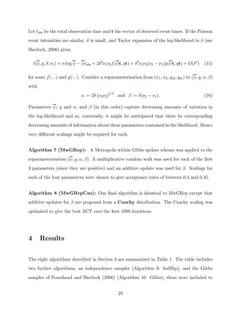
Let tobs be the total observation time and t the vector of observed event times. If the Poisson

event intensities are similar, δ is small, and Taylor expansion of the log-likelihood in δ (see

Sherlock, 2006) gives

l(ψ, q, δ, ν1) = n logψ − ψtobs + 2δ2ν1ν2f(ψt, qt) + δ3ν1ν2(ν2 − ν1)g(ψt, qt) +O(δ4) (15)

for some f(·, ·) and g(·, ·). Consider a reparameterisation from (ψ1, ψ2, q12, q21) to (ψ, q, α, β)

with

α := 2δ (ν1ν2)1/2 and β := δ(ν2 − ν1). (16)

Parameters ψ; q and α; and β (in this order) capture decreasing amounts of variation in

the log-likelihood and so, conversely, it might be anticipated that there be corresponding

decreasing amounts of information about these parameters contained in the likelihood. Hence

very different scalings might be required for each.

Algorithm 7 (MwGRep): A Metropolis within Gibbs update scheme was applied to the

reparameterisation (ψ, q, α, β). A multiplicative random walk was used for each of the first

3 parameters (since they are positive) and an additive update was used for β. Scalings for

each of the four parameters were chosen to give acceptance rates of between 0.4 and 0.45.

Algorithm 8 (MwGRepCau): Our final algorithm is identical to MwGRep except that

additive updates for β are proposed from a Cauchy distribution. The Cauchy scaling was

optimised to give the best ACT over the first 1000 iterations.

4 Results

The eight algorithms described in Section 3 are summarised in Table 1. The table includes

two further algorithms, an independence sampler (Algorithm 9: IndShp), and the Gibbs

sampler of Fearnhead and Sherlock (2006) (Algorithm 10: Gibbs); these were included to

29

No. Abbreviation Description

1 Blk Block additive with tuned proposal N(0, λ2I).

2 MwG Sequential additive with tuned proposals N(0, λ2i ), (i = 1 . . . 4).

3 BlkShp Block additive with tuned proposal N(0, λ2Σ).

4 BlkShpCau Block additive with tuned proposal Cauchy(0, λ2Σ).

5 BlkShpMul Block multiplicative with tuned proposal N(0, λ2Σ).

6 BlkAdpMul Block multiplicative with adaptively tuned mixture proposal.

7 MwGRep Sequential multiplicative/additive Gaussian; reparameterisation.

8 MwGRepCau Sequential multiplicative Gaussian and additive Cauchy; reparameterisation.

9 IndShp Block indepenence sampler with tuned proposal t5(0, Σ).

10 Gibbs Hidden data Gibbs sampler of Fearnhead and Sherlock (2006).

Table 1: Summary of the algorithms used in this paper.

benchmark the efficiency of RWM algorithms against some sensible alternatives. The inde-

pendence sampler used a multivariate t distribution with 5 degrees of freedom and the same

set of covariance matrices as Algorithm 3.

Each RWM variation was tested against data sets D1 and D2 as described in Section 2.3.1.

For each data set, each algorithm was started from the known “true” parameter values and

was run 3 times with 3 different random seeds (referred to as Replicates 1-3). All algorithms

were run for 11000 iterations; a burn in of 1000 iterations was sufficient in all cases.

Priors were independent and exponential with means the known “true” parameter values.

The likelihood of an MMPP with maximum and minimum Poisson intensities ψmax and

ψmin and with n events observed over a time window of length tobs, is bounded above by

ψnmaxe−ψmintobs. In this article only MMPP parameters and their logarithms are considered

for estimation. Since exponential priors are employed the parameters and their logarithms

therefore have finite variance, and geometric ergodicity is guaranteed.

30

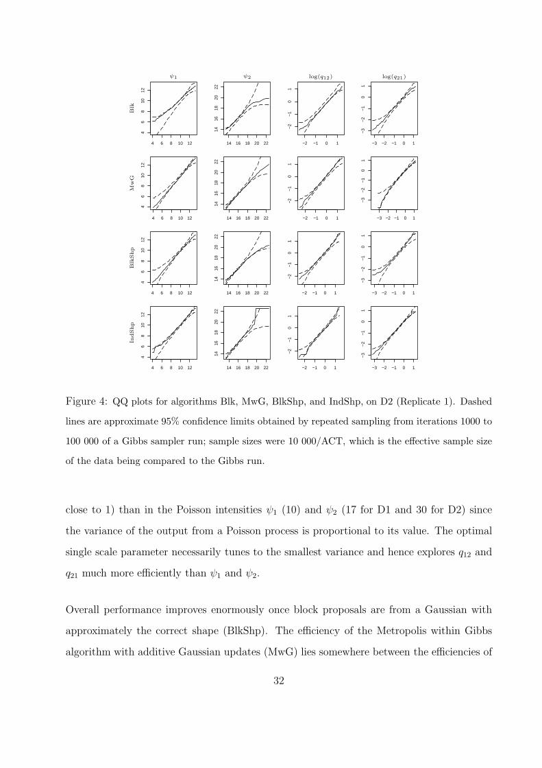
The accuracy of posterior simulations is assessed via QQ plot comparison with the output

from a very long run of a Gibbs sampler (see Section 2.2.3). QQ plots for almost all replicates

were almost entirely within their 95% confidence bounds. Figure 4 shows such plots for

Algorithms 1-3 and 9 (the independence sampler) on data set D2 (Replicate 1). In general

these combinations produced the least accurate performance, and only with the independence

sampler is there reason to doubt that the posterior sample is a reasonable representation of

the true posterior. The relatively poor performance on D2 of Algorithms 1-3, and especially

Algorithm 9 is repeated for the other two replicates. The third replicate of Algorithm 4 on

D2 also showed an imperfect fit in the tails.

The integrated ACT was estimated for each parameter and each replicate using the final 10

000 iterations from that replicate. Calculation of the likelihood is by far the most compu-

tationally intensive operation (taking approximately 99.8% of the total CPU time) and is

performed four times for each Metropolis within Gibbs iteration (once for each parameter)

and only once for each block update; a similar calculation is performed once for each update

of the Gibbs sampelr. To give a truer indication of overall efficiency the ACTs for each

Metropolis within Gibbs replicate have therefore been multiplied by four. Table 2 shows

the mean adjusted ACT for each algorithm, parameter, and data set. For each set of three

replicates most of the ACTs lay within 20% of their mean, and for the exceptions (Blk and

BlkShpCau for data sets D1 and D2, and BlkShp and BlkShpMul for data set D2) full sets

of ACTs are given in Table 3 in Appendix A.

In general all algorithms performed better on D1 than on D2 because, as discussed in Section

2.3.1 data set D1 contains more information on the parameters than D2; it therefore has

lighter tails and is more easily explored by the chain.

The simple block additive algorithm using Gaussian proposals with variance matrix propor-

tional to the identity matrix (Blk) performs relatively poorly on both data sets. In absolute

terms there is much less uncertaintly about the transition intensities q12 and q21 (both are

31

4 6 8 10 124

68

1012

14 16 18 20 22

1416

1820

22

−2 −1 0 1

−2

−1

01

−3 −2 −1 0 1

−3

−2

−1

01

4 6 8 10 12

46

810

12

14 16 18 20 2214

1618

2022

−2 −1 0 1

−2

−1

01

−3 −2 −1 0 1

−3

−2

−1

01

4 6 8 10 12

46

810

12

14 16 18 20 22

1416

1820

22

−2 −1 0 1−

2−

10

1−3 −2 −1 0 1

−3

−2

−1

01

4 6 8 10 12

46

810

12

14 16 18 20 22

1416

1820

22

−2 −1 0 1

−2

−1

01

−3 −2 −1 0 1−

3−

2−

10

1

ψ1 ψ2 log(q12) log(q21)

Blk

Mw

GB

lkShp

IndShp

Figure 4: QQ plots for algorithms Blk, MwG, BlkShp, and IndShp, on D2 (Replicate 1). Dashed

lines are approximate 95% confidence limits obtained by repeated sampling from iterations 1000 to

100 000 of a Gibbs sampler run; sample sizes were 10 000/ACT, which is the effective sample size

of the data being compared to the Gibbs run.

close to 1) than in the Poisson intensities ψ1 (10) and ψ2 (17 for D1 and 30 for D2) since

the variance of the output from a Poisson process is proportional to its value. The optimal

single scale parameter necessarily tunes to the smallest variance and hence explores q12 and

q21 much more efficiently than ψ1 and ψ2.

Overall performance improves enormously once block proposals are from a Gaussian with

approximately the correct shape (BlkShp). The efficiency of the Metropolis within Gibbs

algorithm with additive Gaussian updates (MwG) lies somewhere between the efficiencies of

32

D1 D2

Algorithm ψ1 ψ2 log (q12) log (q21) ψ1 ψ2 log (q12) log (q21)

Blk 66 126 15 19 176 175 80 70

MwG∗ 22 22 33 33 103 90 114 99

BlkShp 13 18 13 15 46 25 37 36

BlkShpCau 19 32 25 24 63 50 56 38

BlkShpMul 13 17 13 15 33 26 22 16

BlkAdpMul 12 12 14 14 20 20 17 23

MwGRep∗ 13 14 32 44 20 23 23 21

MwGRepCau∗ 14 15 37 42 24 233 25 23

IndShp+ 3.7 5.5 3.5 3.7

Gibbs 4.2 3.2 5.7 5.9 26 19 32 27

Table 2: Mean estimated integrated autocorrelation time for the four parameters over three

independent replicates for data sets D1 and D2. ∗Estimates for MwG replicates have been

multiplied by 4 to provide figures comparable with full block updates in terms of CPU time.

+ ACT results for the independence sampler for D2 are irrelevant since the MCMC sample

was not an accurate representation of the posterior.

Blk and BlkShp but the improvement over Blk is larger for data set D1 than for data set

D2. As discussed in Section 2.3.1 the parameters in D1 are more nearly independent than

the parameters in D2. Thus for data set D1 the principal axes of an elliptical approximation

to the posterior are more nearly parallel to the cartesian axes. Metropolis-within-Gibbs

updates are (by definition) parallel to each of the cartesian axes and so can make large

updates almost directly along the major axis of the ellipse for data set D1.

For the heavy tailed posterior of data set D2 we would expect block updates resulting from

a Cauchy proposal (BlkShpCau) to be more efficient than those from a Gaussian proposal.

However for both data sets Cauchy proposals are slightly less efficient than Gaussian propos-

33

als. It is likely that the heaviness of the Cauchy tails leads to more proposals with at least

one negative parameter, such proposals being automatically rejected. Moreover Σ represents

the main posterior mass, yet some large Cauchy jump proposals from this mass will be in

the posterior tail. It may be that Σ does not accurately represent the shape of the posterior

tails.

Multiplicative updates (BlkShpMul) make little difference for D1, but for the relatively

heavy tailed D2 there is a definite improvement over BlkShp. The adaptive multiplicative

algorithm (BlkAdpMul) is slightly more efficient still, since the estimated variance matrix

and the overall scaling are refined thoughout the run.

As was noted earlier in this section, due to our choice of exponential priors the quantities

estimated in this article have exponential or lighter posterior tails and so all the non-adaptive

algorithms in this article are geometrically ergodic. The theory in Section 3.4 suggests ways

to improve tail exploration for polynomially ergodic algorithms and so, strictly speaking,

need not apply here. However the exponential decay only becomes dominant some distance

from the posterior mass, especially for data set D2. Polynomially increasing terms in the

likelihood ensure that initial decay is slower than exponential, and that the multiplicative

random walk is therefore more efficient than the additive random walk.

The adaptive overall scaling m showed variability of O(0.1) over the first 1000 iterations

after which time it quickly settled down to 1.2 for all three replicates on D1 and to 1.1 for all

three replicates on D2. Both of these values are very close to the scaling of 1.19 that would

be used for a four dimensional update in the scheme of Roberts and Rosenthal (2009). The

algorithm similarly learnt very quickly about the variance matrix Σ, with individual terms

settling down after less than 2000 iterations, and with exploration close to optimal after less

than 500 iterations. This can be seen clearly in Figure 5 which shows trace plots for the first

2000 iterations of the first replicate of BlkAdpMul on D2.

34

0 500 1000 1500 2000

68

10

12

Index

0 500 1000 1500 2000

14

16

18

20

22

Index

0 500 1000 1500 2000

−2

−1

01

Index

0 500 1000 1500 2000

−2

.0−

1.0

0.0

1.0

Index

ψ1

ψ2

log(q

12)

log(q

21)

Figure 5: Trace plots for the first 2000 iterations of BlkAdpMul on data set D2 (Replicate 1).

The adaptive algorithm uses its own history to learn about d(d+1)/2 covariance terms and a

best overall scaling. One would therefore expect that the larger the number of parameters, d,

the more iterations are required for the scheme to learn about all of the adaptive terms and

hence reach a close to optimal efficiency. To test this a data set (D3) was simulated from a

three-dimensional MMPP with ψ = [10, 17, 30]t and q12 = q13 = q21 = q23 = q31 = q32 = 0.5.

The following adaptive algorithm was then run three times, each for 20 000 iterations.

Algorithm 6b (BlkAdpMul(b)): This adaptive algorithm is identical to BlkAdpMul

(with d = 9) except that no adaptive proposals were used until at least 100 non-adaptive

proposals had been accepted, and that if an adaptive proposal was accepted then the overall

scaling was updated with m ← m + 3 ∆/i1/2 so that the equilibrium acceptance rate was

approximately 0.25.

Figure 6 shows the evolution of four of the forty six adaptive parameters (Replicate 1). All

parameters seem close to their optimal values after 10 000 iterations, although covariance

35

0 5000 10000 15000 20000

0.0

0.2

0.4

0.6

0.8

1.0

1.2

Index

0 5000 10000 15000 20000

0.0

00

0.0

02

0.0

04

0.0

06

Index

0 5000 10000 15000 20000

0.0

1.0

2.0

3.0

Index

0 5000 10000 15000 20000

−0

.04

−0

.02

0.0

0

Index

m

Var[logψ

1]

Var[logq12]

Cov[ψ

1,q12]

Figure 6: Plots of the adaptive scaling parameter m and three estimated covariance parameters

Var [ψ1], Var [q12], and Cov [ψ1, q12] for BlkAdpMul(b) on data set D3 (Replicate 1).

parameters appear to be still slowly evolving even after 20 000 iterations. In contrast, trace

plots of parameters (not shown) reveal that the speed of exploration of the posterior is close

to its final optimum after only 1500 iterations. This behaviour was repeated across the other

two replicates, indicating that, as with the two-dimensional adaptive and non-adaptive runs,

even a very rough approximation to the variance matrix improves efficiency considerably.

Over the full 20 000 iterations, all three replicates showed a definite multimodality with λ2

often close to either λ1 or λ3, indicating that the data might reasonably be explained by a

two dimensional MMPP. In all three replicates the optimal scaling settled between 0.25 and

0.3, noticeably lower than Roberts and Rosenthal (2009) value of 2.38/√

9. With reference to

Section 3.1 this is almost certainly due to the roughness inherent in a multimodal posterior.

The reparameterisation of Section 3.5.2 was designed for data sets similar to D2, and on this

data set the resulting Metropolis within Gibbs algorithm (MwGRep) is at least as efficient

as the adaptive multiplicative random walk. On data set D1 however exploration of q12 and

36

q21 is arguably less efficient than for the Metropolis within Gibbs algorithm with the original

parameter set. The lack of improvement when using a Cauchy proposal for β (MwGRepCau)

suggests that this inefficiency is not due to poor exploration of the potentially heavy tailed

β. Further investigation in the (ψ, q, α, β) parameter space showed that for data set D1

only q was explored efficiently; the posteriors of ψ and β were strongly positively correlated

(ρ ≈ 0.8), and both ψ and β were strongly negatively correlated with α (ρ ≈ −0.65).

Posterior correlations were small |ρ| < 0.3 for all parameters with data set D2 and for all

correlations involving q for data set D1.

The optimal scaling for the one-dimensional additive Cauchy proposal in MwGRepCau was

approximately two thirds of the optimal scaling for the one-dimensional additive Gaussian

proposal in MwGRep. In four dimensions the ratio was approximately one half. These ratios

allow the Cauchy proposals to produce similar numbers of small to medium sized jumps to

the Gaussian proposals.

The independence sampler is arguably the most efficient of all of the algorithms considered

for D1. However, as discussed earlier in this section, there are doubts about the accuracy of

its exploration of D2. Mengersen and Tweedie (1996) show that an independence sampler

is uniformly ergodic if and only if the ratio of the proposal density to the target density is

bounded below, and that one minus this ratio gives the geometric rate of convergence. To

ensure the lower bound it is advisable to propose from a relatively heavy-tailed distribution,

such as the t5 used here. The problem in this instance arises because dataset D2 could, just

possibly, have been generated by a single Poisson process with intensity ψ ≈ (ψ1 + ψ2)/2.

The resulting minor mode (or, more precisely, ridge) is some distance from the centre of the

distribution, resulting in a low ratio of proposal and target densities.

The Gibbs sampler of Fearnhead and Sherlock (2006) is accurate, with its efficiency directly

related to the amount of information about the hidden Markov chain that is available from

the data (Sherlock, 2006). Thus for D1 the Gibbs sampler is more efficient than the best

37

RWM algorithms, but this is not the case for D2.

5 Discussion

We have described the theory and intuition behind a number of techniques for improving the

efficiency of random walk Metropolis algorithms and tested these on two data sets generated

from Markov modulated Poisson processes (MMPPs). Tests on these data sets also showed

a sensibly implemented RWM to be at least as good as some of the other available MCMC

algorithms. Some RWM implementations were uniformly successful at improving efficiency,

whilst for others success depended on the shape and/or tails of the posterior. All of the

underlying concepts discussed here are quite general and easily applied to statistical models

other than the MMPP.

Simple acceptance rate tuning to obtain the optimal overall variance term for a symmetric

Gaussian proposal can increase efficiency by many orders of magnitude. However with our

data sets, even after such tuning, the RWM algorithm was very inefficient. The effectiveness

of the sampling increased enormously once the shape of the posterior was taken into account

by proposing from a Gaussian with variance proportional to an estimate of the posterior

variance. For Algorithms 3, 4 and 5 the posterior variance was estimated though a short

“training run” - the first 1000 iterations after burn-in of Algorithm 1.

As expected, use of the “multiplicative random walk” (Algorithm 5), a random walk on

the posterior of the logarithm of the parameters, improved efficiency most noticeably on

the posterior with the heavier tails. However, contrary to expectation, even on the heavier

tailed posterior an additive Cauchy proposal (Algorithm 4) was, if anything, less efficient

than a Gaussian. Tuning of Cauchy proposals was also more time-consuming since simple

acceptance rate criteria could not be used.

38

Algorithm 6 combined the successesful strategies of optimal scaling, shape tuning, and trans-

forming the data, to create a multiplicative random walk which learned the most efficient

shape and scale parameters from its own history as it progressed. This adaptive scheme

was easy to implement and was arguably the most efficient RWM for each of the data sets.

A slight variant of this algorithm was used to explore the posterior of a three-dimensional

MMPP, and showed that in higher dimensions such algorithms take longer to discover close

to optimal values for the adaptive parameters. These runs also confirmed the finding for the

two dimensional MMPP that RWM efficiency improves enormously with knowledge of the

posterior variance, even if this knowledge is only approximate. For a multimodal posterior

such as that found for the three-dimensional MMPP it might be argued that a different vari-

ance matrix should be used for each mode. Such “regionally adaptive” algorithms present

additional problems, such as the definition of the different regions, and are discussed further

in Roberts and Rosenthal (2009).

Metropolis within Gibbs updates performed better when the parameters were close to orthog-

onal, at which point the algorithms were almost as efficient as an equivalent block updating

algorithm with tuned shape matrix. The best Metropolis within Gibbs scheme for data set

D2 arose from a new reparameterisation devised specifically for the two dimensional MMPP

with parameter orthogonality in mind. On D2 this performed nearly as well as the best

scheme, the adaptive multiplicative random walk.

The adaptive schemes discussed here provide a significant step towards a goal of completely

automated algorithms. However, as already discussed, for d model-parameters, a posterior

variance matrix has O(d2) components. Hence the length of any “training run” or of the

adaptive “learning period” increases quickly with dimension. For high dimension it is there-

fore especially important to utilise to the full any problem specific knowledge that is available

so as to provide as efficient a starting algorithm as possible.

39

A Runs with highly variable ACTs

Three replicates were performed for each data set and algorithm, and ACTs are summarised

by their mean in Table 2. However for certain combinations the algorithms and data sets

the ACTs varied considerably; full sets of ACTs for these replicates are given in Table 3.

Algorithm ψ1 ψ2 log (q12) log (q21)

Blk (D1) 59,64,75 120,155,104 12,15,17 19,21,17

BlkShpCau (D1) 28,16,12 36,29,31 20,20,35 26,23,24

Blk (D2) 121,259,146 107,262,157 41,139,61 51,110,48

BlkShp (D2) 54,51,34 23,24,29 40,45,27 50,35,23

BlkShpCau (D2) 46,51,92 46,57,48 31,42,94 39,41,34

BlkShpMul (D2) 53,24,23 22,33,25 20,23,24 17,18,13

Table 3: Estimated ACT for the four parameters, on three independent replicates for Blk

and BlkShpCau on data set D1 and Blk, BlkShp, BlkShpCau and BlkShpMul on D2.

References

Bai, Y., Roberts, G. O. and Rosenthal, J. S. (2009). On the containment condition for

adaptive Markov chain Monte Carlo algorithms. Submitted Preprint.

Bedard, M. (2007). Weak convergence of Metropolis algorithms for non-i.i.d. target distri-

butions. Ann. Appl. Probab. 17(4), 1222–1244.

Bedard, M. (2008). Optimal acceptance rates for Metropolis algorithms: moving beyond

0.234. Stochastic Process. Appl. 118(12), 2198–2222.

Burzykowski, T., Szubiakowski, J. and Ryden, T. (2003). Analysis of photon count data

from single-molecule fluorescence experiments. Chemical Physics 288, 291–307.

40

Carlin, B. P. and Louis, T. A. (2009). Bayesian methods for data analysis . Texts in Statistical

Science Series, CRC Press, Boca Raton, FL, 3rd edition.

Dellaportas, P. and Roberts, G. O. (2003). An introduction to MCMC. In: Spatial Statistics

and Computational Methods (ed. J. Moller), number 173 in Lecture Notes in Statistics,

Springer, Berlin, 1–41.

Fearnhead, P. and Sherlock, C. (2006). An exact Gibbs sampler for the Markov modulated

Poisson processes. J. R. Stat. Soc. Ser. B Stat. Methodol. 68(5), 767–784.

Gamerman, D. and Lopes, H. F. (2006). Markov chain Monte Carlo. Texts in Statistical

Science Series, Chapman & Hall/CRC, Boca Raton, FL, 2nd edition, stochastic simulation

for Bayesian inference.

Geyer, C. J. (1992). Practical Markov chain Monte Carlo. Statistical Science 7, 473–483.

Gilks, W. R., Richardson, S. and Spiegelhalter, D. J. (1996). Markov Chain Monte Carlo in

practice. Chapman and Hall, London, UK.

Jarner, S. F. and Roberts, G. O. (2002). Polynomial convergence rates of Markov chains.

Ann. Appl. Probab. 12(1), 224–247.

Kou, S. C., Xie, X. S. and Liu, J. S. (2005). Bayesian analysis of single-molecule experimental

data. Appl. Statist. 54, 1–28.

Mengersen, K. L. and Tweedie, R. L. (1996). Rates of convergence of the Hastings and

Metropolis algorithms. Ann. Statist. 24(1), 101–121.

Metropolis, N., Rosenbluth, A. W., Rosenbluth, M. N., Teller, A. H. and Teller, E. (1953).

Equations of state calculations by fast computing machine. J. Chem. Phys. 21, 1087–1091.

Meyn, S. P. and Tweedie, R. L. (1993). Markov chains and stochastic stability . Communi-

cations and Control Engineering Series, Springer-Verlag London Ltd., London.

41

Neal, P. and Roberts, G. (2006). Optimal scaling for partially updating MCMC algorithm.

Ann. Appl. Probab. 16, 475–515.

Roberts, G. O. (2003). Linking theory and practice of MCMC. In: Highly structured stochas-

tic systems , volume 27 of Oxford Statist. Sci. Ser., Oxford Univ. Press, Oxford, 145–178,

with part A by Christian P. Robert and part B by Arnoldo Frigessi.

Roberts, G. O. and Rosenthal, J. S. (2001). Optimal scaling for various Metropolis-Hastings

algorithms. Statistical Science 16, 351–367.

Roberts, G. O. and Rosenthal, J. S. (2007). Coupling and ergodicity of adaptive Markov

chain Monte Carlo algorithms. J. Appl. Probab. 44(2), 458–475.

Roberts, G. O. and Rosenthal, J. S. (2009). Examples of adaptive MCMC. J. Comp. Graph.

Stat. To appear.

Roberts, G. O., Gelman, A. and Gilks, W. R. (1997). Weak convergence and optimal scaling

of random walk Metropolis algorithms. The Annals of Applied Probability 7, 110–120.

Scott, S. L. and Smyth, P. (2003). The Markov modulated Poisson process and Markov

Poisson cascade with applications to web traffic modelling. Bayesian Statistics 7, 1–10.

Sherlock, C. (2005). In discussion of ’Bayesian analysis of single-molecule experimental data’.

Journal of the Royal Statistical Society, Series C 54, 500.

Sherlock, C. (2006). Methodology for inference on the Markov modulated Poisson process

and theory for optimal scaling of the random walk Metropolis. Ph.D. thesis, Lancaster

University, available from http://eprints.lancs.ac.uk/850/.

Sherlock, C. and Roberts, G. (2009). Optimal scaling of the random walk Metropolis on

elliptically symmetric unimodal targets. Bernoulli 15(3), 774–798.

Sokal, A. (1997). Monte Carlo methods in statistical mechanics: foundations and new algo-

rithms. In: Functional integration (Cargese, 1996), volume 361 of NATO Adv. Sci. Inst.

Ser. B Phys., Plenum, New York, 131–192.

42