Embed Size (px)
Citation preview
The Rangeland Hydrology and Erosion Model: A Dynamic Approach for Predicting 1 Soil Loss on Rangelands 2
3
Mariano Hernandez1, Mark A. Nearing1, Osama Z. Al-Hamdan2, Frederick B. Pierson3, 4 Gerardo Armendariz1, Mark A. Weltz4, Kenneth E. Spaeth5, C. Jason Williams1, and Carl 5 L. Unkrich1 6
1USDA, Agricultural Research Service, Southwest Watershed Research Center, Tucson, 7 Arizona, USA 8 2Texas A&M University-Kingsville, Kingsville, Texas, USA 9 3USDA, Agricultural Research Service, Northwest Watershed Research Center, Boise, Idaho, 10 USA 11 4USDA, Agricultural Research Service, Exotic and Invasive Weeds Research Unit, Reno, 12 Nevada, USA 13 5USDA, Natural Resources Conservation Service, Central National Technology Support Center, 14 Ft. Worth, Texas, USA 15
Corresponding author: Mariano Hernandez ([email protected]) 16
Key Points: 17
• List up to three key points (at least one is required) 18
• Key Points summarize the main points and conclusions of the article 19
• Each must be 140 characters or less with no special characters or acronyms. 20 21
The Rangeland Hydrology and Erosion Model (RHEM) is a process-based erosion 22 prediction tool specific for rangeland application, based on fundamentals of infiltration, 23 hydrology, hydraulics, and erosion mechanics. RHEM captures the influence of plant 24 lifeform type, vegetation foliar and ground cover, rock cover, slope steepness, soil texture, 25 and rainfall on the dominant erosion processes on rangelands. The model utilizes a partial 26 differential equation that solves in downslope distance and time during the event. Here we 27 present the new dynamic model and evaluate it against 23 observed runoff and sediment 28 events collected in a shrub-dominated semiarid watershed in the Arizona, USA. To 29 evaluate the model, primary model parameters were determined using RHEM parameter 30 estimation equations. Second, the model was calibrated to measurements from the 31 watershed. The parameters estimated by the parameter estimation equations were within 32 the lowest and highest values of the calibrated parameter set. Third, 124 data points in 33 Arizona and New Mexico were used to evaluate runoff and erosion as a function of foliar 34 canopy cover and ground cover. The dependence of average sediment yield on surface 35 ground cover was moderately stronger than that on foliar canopy cover. The RHEM 36 model is shown to track runoff volume, peak runoff, and sediment yield with sufficient 37 accuracy for operational use of the model. 38
39
1 Introduction 40 The complex interactions of climate change processes, vegetation characteristics, surface soil 41
processes, and human activities have major impacts on runoff and soil erosion processes on 42 rangeland ecosystems. These processes and activities affect ecosystem function over a wide 43 range of spatial and temporal scales [Williams et al., 2016]. Nearing et al. [2004] suggested that 44 climatic variability will increase in the future. That is, global warming is expected to lead to a 45 more vigorous hydrological cycle, including total rainfall and more frequent high-intensity 46 rainfall events [Nearing et al., 2004]. Rangeland degradation is more likely to occur during these 47 extreme rainfall events. Decades of research have shown that rangelands can sustainably produce 48 a variety of goods and services even in the face of extreme climatic events if managers respond 49 quickly and appropriately to changes [Havstad et al., 2009]. While individual ranchers may not 50 be able to reduce the progress of climate change through mitigation, they may be able to adjust to 51 climate change and devise management practices that are more resilient to climate impacts. Soil 52 erosion is among the climate-related impacts that concern rangeland managers since 53 conservation of topsoil is critical to sustained productivity in rangeland ecosystems. Soil loss 54 rates on rangelands are regarded as one of the few quantitative indicators for assessing rangeland 55 health and conservation practice effectiveness [Nearing et al., 2011]. 56 57
According to Briske et al. [2011], the environmental benefits of grazing lands conservation 58 practices have not previously been quantified at a national scale. The Rangeland Conservation 59 Effects Assessment Project (CEAP) was formally initiated in 2006 to evaluate conservation 60 effectiveness on rangelands and grazed forest that together comprise 188 million hectares of 61 USA nonfederal rural land, as well as large areas of federal land in the western United States. 62 Broad-scale assessments of this type rely on reliable modeling capabilities. According to 63 Nearing and Hairsine [2011], future erosion prediction technology must be capable of simulating 64 the complex interactions between vegetation characteristics, surface soil properties and 65

hydrologic and erosion processes on rangelands. Furthermore, Al-Hamdan et al. [2012b] pointed 66 out that better representation of the temporal dynamics of soil erodibility related to disturbed 67 rangeland conditions (e.g., fire) is also needed. 68
69 In 2006, the USDA-Agricultural Research Service (USDA-ARS) developed the Rangeland 70
Hydrology and Erosion Model (RHEM) V1.0 based on state-of-the-art technology from the 71 Water Erosion Prediction Project (WEPP) [Flanagan and Nearing, 1995]. However, the basic 72 equations in the WEPP model are based on experimental data from croplands. While many of the 73 fundamental hydrologic and erosion processes can be expressed in a common way on both crop 74 and rangelands, there were several aspects of the WEPP model that are not optimum for 75 rangeland application and were modified, dropped, or replaced in RHEM [Nearing et al., 2011]. 76 77
RHEM V1.0 was initially developed for undisturbed rangelands where the impact of 78 concentrated flow erosion is limited and most soil loss occurs by rain splash and sheet erosion 79 processes. RHEM V1.0 included a new splash and sheet equation developed by Wei et al. [2009] 80 based on rainfall simulation data collected on rangeland plots from the WEPP and IRWET 81 [IRWET and NRST, 1998] projects, which together covered 49 rangeland sites distributed across 82 15 western states. Also, it was incorporated the full solution to the kinematic wave equation for 83 overland flow routing instead of the approximate method for calculating peak runoff 84 implemented in WEPP [Stone et al., 1992]. Furthermore, RHEM V1.0 adapted the WEPP's 85 steady state cropland-based shear stress approach for modeling concentrated flow erosion. 86 Consequently, it was not possible to quantify within-storm sediment dynamics [Bulygina et al., 87 2007]. That is, a steady state model does not provide information on peak sediment discharge or 88 the sediment load pattern within the storm, both of which can be useful for assessing potential 89 pollution loadings from sediment fluxes into water courses and identifying sediment sources for 90 designing appropriate management alternatives that reduce sediment losses [Kalin et al., 2004]. 91 RHEM V1.0 uses the shear stress partitioning detachment and deposition concepts developed by 92 Foster [1982], which distributes the transport capacity among various particle types. 93 94
The enhanced RHEM V2.3 model discussed herein provides major advantages over existing 95 erosion model prediction technology, including RHEM V1.0. RHEM V2.3 is capable of 96 capturing the influence of different plant types, disturbances such as fire, climate change, and 97 rangeland management practices on important erosion processes acting on rangelands. RHEM 98 has undergone continued review and expansion of capabilities. The most significant between this 99 model and the original are: (1) The model uses a dynamic solution of the sediment continuity 100 equation based on kinematic wave routing of runoff, and the integration of the newly developed 101 splash and sheet source term equation and stream power for predicting sediment transport of 102 concentrated flow erosion. (2) It integrates the approach for estimating the splash and sheet 103 erodibility coefficient formulated by Al-Hamdan et al. [2016], who developed equations to 104 predict the differences of erodibility before and after disturbance across a wide range of soil 105 texture classes and vegetation cover types. (3) The model integrates the method for predicting 106 concentrated flow erosion based on the work by Al-Hamdan et al. [2013], who developed a 107 dynamic erodibility approach for modeling concentrated flow erosion (e.g., for sites with 108 relatively immediate disturbance, such as fire). (4) The model includes a user-friendly web-based 109 interface to allow users to simplify the use of RHEM, manage scenarios, centralize scenario 110

results, compare scenario results, and provide tabular and graphical results [Hernandez et al., 111 2015]. 112
113 RHEM has been applied successfully to illustrate the influence of plant and soil 114
characteristics on soil erosion and hydrologic function in MLRA 41 located in Southeastern 115 Basin and Range region of the southern U.S. [Hernandez et al., 2013]; assess non-federal 116 western rangeland soil loss rates at the national scale for determining areas of vulnerability for 117 accelerated soil loss using USDA Natural Resources Conservation Services(NRCS) National 118 Resources Inventory(NRI) data [Weltz et al., 2014]; predict runoff and erosion rates for 119 refinement and development of Ecological Site Descriptions [Williams et al., 2016]; characterize 120 rangeland conditions based on a probabilistic approach subject to the presence of a set of soil 121 erosion thresholds [Hernandez et al. 2016]. 122
123 The objectives of this study were as follows. (1) to present the driving equations for the 124
new RHEM V2.3 model; (2) to calibrate the new RHEM V2.3 model using 23 rainfall-runoff-125 sediment yield events on a small semiarid sub-watershed within the Walnut Gulch Experimental 126 Watershed in Arizona, and compare them against parameters estimated by the RHEM parameter 127 estimation equations; (3) to examine the ranges of parameter values from RHEM parameter 128 estimation equations and compare them to calibrated parameter values; (4) to evaluate the overall 129 influence of foliar canopy cover, ground surface cover, and annual rainfall on soil erosion rates 130 from rangelands using 124 NRI plots in Arizona and New Mexico. 131
132 2. Material and Methods 133 134
This section is divided into four main parts as follows. (1) Presentation of fundamental 135 hydrologic and erosion equations in RHEM, (2) An overview of the RHEM parameter estimation 136 equations, (3) Model calibration with the Model-Independent Parameter ESTimation (PEST) 137 program, (4) Statistical analysis. 138 139 2.1. Fundamental hydrologic and erosion equations 140 141 2.1.1. Overland flow model 142 143
The hydrology component of the enhanced RHEM model is based on the KINEROS2 144 model [Smith et al., 1995]. The model was implemented to simulate one-dimensional overland 145 flow within an equivalent plane representing an arbitrarily shaped hillslope with uniform or 146 curvilinear slope profiles. The flow per unit width across a plane surface as a result of rainfall 147 can be described by the one-dimensional continuity equation [Woolhiser et al. 1990]. 148 149
𝜕ℎ𝜕𝑡 +
𝜕𝑞𝜕𝑥 = s 𝑥, 𝑡 (1) 150
151 where h is the flow depth at time t and the position x; x is the space coordinate along the 152 direction of flow; q is the volumetric water flux per unit plane width (m2 s-1); and s (x, t) is the 153 rainfall excess (m s-1). 154
155 s 𝑥, 𝑡 = 𝑟 − 𝑓 (2) 156
157 where r is the rainfall rate (m s-1), and f is the infiltration rate (m s-1). The following equation 158 represents the relationship between q and h: 159 160
𝑞 =8𝑔𝑆𝑓4
56ℎ7 6 (3) 161
162 where g is the gravity acceleration (m s-2), S is the slope (m m-1), and ft is the total friction factor 163 estimated by [Al-Hamdan et al., 2013]. Substituting Equations (2) and (3) in Equation (1) results 164 in the hydrology routing equation: 165 166
𝜕ℎ𝜕𝑡 +
328𝑔𝑆𝑓4
56ℎ5 6
𝜕ℎ𝜕𝑥 = 𝑟 − 𝑓 (4) 167
168 In RHEM, for a single plane, the upstream boundary is assumed to be at zero depth and the 169 downstream boundary is a continuing plane (along the direction of flow). 170
171 ℎ 0, 𝑡 = 0 (5) 172
173 The infiltration rate is computed in KINEROS2 using the three-parameter infiltration 174
equation [Parlange et al., 1982], in which the models of Green and Ampt [1911] and Smith and 175 Parlange [1978] are included as two limiting cases. 176 177
𝑓 = 𝐾= 1 +a
𝑒𝑥𝑝 ∝ 𝐼𝐺Δ𝜃E
− 1 (6) 178
179 where I is the cumulative depth of the water infiltrated into the soil (m), Ke is the surface 180 effective saturated hydraulic conductivity (m s-1), G (m) accounts for the effect of capillary 181 forces on moisture absorption during infiltration, and a is a scaling parameter. When a=0, 182 Equation 6 is reduced to the simple Green and Ampt infiltration model, and when a=1, the 183 equation simplifies to the Parlange model. Most soil exhibit infiltrability behavior intermediate 184 to these two models, and KINEROS2 uses a weighting a value of 0.85 [Smith et al., 1993]. The 185 state variable for infiltrability is the initial water content, in the form of the soil saturation deficit, 186 𝐵 = 𝐺 𝜃H − 𝜃E , defined as the saturated moisture content minus the initial moisture content. 187 The saturation deficit (𝜃H − 𝜃E) is one parameter because θs is fixed from storm to storm. For 188 ease of estimation, the KINEROS2 input parameter for soil water is a scaled moisture content, 189 S=θ/ϕ, (ϕ is the soil porosity) which varies from 0 to 1. Thus initial soil conditions are 190 represented by the variable Si (=θi/ϕ). Thus, there are two parameters, Ke, and G to characterize 191 the soil, and the variable Si to characterize the initial condition 192
193 2.1.2. Overland soil erosion, deposition, and transport 194 195 The RHEM erosion model uses a dynamic sediment continuity equation to describe the 196 movement of suspended sediment in a concentrated flow area [Bennett, 1974]. 197
198 𝜕 𝐶ℎ𝜕𝑡 +
𝜕 𝐶𝑞J𝜕𝑥 = 𝐷HH + 𝐷LM (7) 199
200 Where C is the measured sediment concentration (kg m-3), qr is the flow discharge of 201 concentrated flow per unit width (m-2 s-1), Dss is the splash and sheet detachment rate (kg s-1 m-1), 202 and Dcf is the concentrated flow detachment rate (kg s-1 m-2). For a unit wide plane, when 203 overland flow accumulates into a concentrated flow path, the following equation calculates the 204 concentrated flow discharge per unit width (qr): 205 206
𝑞J =𝑞𝑤 (8) 207
208 Where w is the concentrated flow width (m) calculated by [Al-Hamdan et al., 2012a] 209 210
𝑤 =2.46 𝑄R.7S
𝑆R.T (9) 211 212 The splash and sheet detachment rate (Dss) is calculated by the following equation [Wei et al., 213 2009]: 214 215
𝐷HH = 𝐾HH𝑟5.RV6𝜎R.VS6 (10) 216 217 where Kss is the splash and sheet erodibility, r (m s-1) is the rainfall intensity and σ is rainfall 218 excess (m s-1). 219 220 Concentrated flow detachment rate (Dcf) is calculated as the net detachment and deposition rate 221 [Foster, 1982]: 222 223
𝐷LM = 𝐷L 1 −
𝐶𝑄𝑇L
, 𝐶𝑄 ≤ 𝑇L
0.5 𝑉M𝑄 𝑇L − 𝐶𝑄 , 𝐶𝑄 ≥ 𝑇L
(11) 224
225 where Dc is the concentrated flow detachment capacity (kg s-1 m-2); Q is the flow discharge (m3 s-226 1); Tc is the sediment transport capacity (kg s-1); and Vf is the soil particle fall velocity (m s-1) that 227 is calculated as a function of particle density and size [Fair et al., 1971]. 228 229
Sediment detachment rate from the concentrated flow is calculated by employing soil 230 erodibility characteristics of the site and hydraulic parameters of the flow such as flow width and 231
stream power. Soil detachment is assumed to start when concentrated flow starts (i.e. no 232 threshold concept for initiating detachment is used) [Al-Hamdan et al., 2012b]. 233
234 To calculate Dc, the equation developed by Al-Hamdan et al. [2012b] is used: 235
236 𝐷L = 𝐾\ 𝑤 (12) 237
238 where Kw is the stream power erodibility factor (s2 m-2) and w is the stream power (kg s-3). We 239 implemented the empirical equation developed by Nearing et al. [1997] to calculate the transport 240 capacity (Tc). 241 242
𝐿𝑜𝑔5R10𝑇L𝑤 = −34.47 + 38.61 ∗
𝑒𝑥𝑝 0.845 + 0.412 log 1000𝑤1 + 𝑒𝑥𝑝 0.845 + 0.412 log 1000𝑤 (13) 243
244 Soil detachment is assumed to be a nonselective process, so the sediment particles size 245
distribution generated from actively eroding areas is assumed to be a function of the fraction of 246 total sediment load represented by five particle classes based on soil texture. The transport 247 capacity equation of Nearing et al. [1997] does not account for particle sorting. Consequently, 248 routing of sediment by size particle is not carried out. 249 250
Several studies have documented increases in peak flows and erosion occurring on 251 systems that have been altered by some disturbance. For example, at the plot/hillslope scale, 252 factor increases in sediment delivery between 2- and 1000 -fold have been reported [Morris and 253 Moses, 1987; Scott and Van Wyk, 1992; Shakesby et al., 1993; Cerda, 1998; Cannon et al., 254 2001; Pierson et al., 2002]. Results from rainfall simulator experiments suggest that erosion rates 255 are much higher in the early part of a runoff event than in the latter part of the event on forest 256 roads [Foltz et al., 2008] and burned rangeland [Pierson et al., 2008]. These rapid changes in the 257 concentrated flow erosion rate on disturbed soils may be caused by the winnowing of fine or 258 easily detached soil particles during the early stages of erosive runoff, thus leaving larger or 259 more embedded particles and/or aggregates which require greater stream power for detachment 260 [Robichaud et al., 2010]. 261
262 RHEM also has the capacity, as an option, to use equations developed by Al-Hamdan et 263
al. [2012b] for characterizing events with high concentrated flow erodibility at the onset of the 264 event with exponentially decreasing erodibility because of the reduction of the availability of 265 disturbance generated sediment. 266
267 𝐷L = 𝐾\ cde dfg𝑒𝑥𝑝 𝛽 𝑞L 𝜔 (14) 268
269
𝑞L = 𝑞J𝑑𝑡 (15) 270
271 𝜔 = 𝛾𝑆𝑞J (16) 272
273 where Kw(Max)adj is the maximum stream power erodibility (s2 m-2) corresponding to the decay 274 factor b = -5.53 (m-2), b is a decay coefficient representing erodibility change during an event 275
(m-2), w is the stream power (kg s-3), qc is the cumulative flow discharge of concentrated flow per 276 unit width (m2), g is the water specific weight (kg m-2 s-2), and S is the slope (m m-1). 277 278 279 2.2. RHEM Model Parameter Estimation Equations 280 281
An important aspect of RHEM about the application by rangeland managers is that it is 282 parameterized based on plant growth form types using data that are typically collected for 283 rangeland management processes (e.g. rangeland health or NRI assessments). 284
285 2.2.1. Effective saturated hydraulic conductivity 286 287
Research has indicated that infiltration, runoff, and erosion dynamics are correlated with 288 the presence/absence and composition of specific plant taxa and growth attributes [Davenport et 289 al., 1998, Wainwright et al., 2000, Ludwig et al., 2005, Peters et al., 2007, Turnbull et al., 2008, 290 Turnbull et al., 2012, Petersen et al., 2009, Pierson et al., 2010, Pierson et al., 2013, Wilcox et 291 al., 2012a and Williams et al., 2014]. It has been known that infiltration of rainfall on rangelands 292 is increased with an increase of vegetal surface cover present. Tromble et al. [1974] evaluated 293 infiltrability on three range sites in Arizona and found vegetal cover and litter biomass to be most 294 positively related, whereas gravel cover was negatively related. Meeuwig [1970] and Dortignac 295 and Love [1961] also found litter cover to be important. Work by Spaeth et al. [1996] concluded 296 that plant species and ground cover effects significantly enhanced estimation of infiltration 297 capacity compared to purely physically based predictions. The study by Thompson et al. [2010] 298 provides a detail literature review about research that has been conducted concerning vegetation-299 infiltration relationships across climate and soil type gradients. 300 301
Soil texture may be used as the first estimator of Ke because texture affects the pore space 302 available for water movement. Also, soil texture is easy to measure and often available for an 303 area of interest. Rawls et al. [1982] developed a look-up table of Ks values for the 11 USDA soil 304 textural classes. Bulk density is another basic soil property that is related to pore space and water 305 movement. Rawls et al. [1998] revised the texture-based look-up table to include two porosity 306 classes within each textural class, the geometric means of the Ks along with the 25% and 75% 307 percentile values. The texture/porosity Ks estimates were based on a national database of 308 measured Ks values and soil properties at 953 locations. These estimates indicate that (1) Ks is 309 highest for coarse-textured soils and (2) within a textural class, soils with greater porosity (lower 310 bulk density) have higher Ks values. 311 312
The geometric mean of Ks sorted according to the soil texture, and bulk density classes 313 along with the 25% and 75% percentile values are presented in Table 3. Also, reported in Table 1 314 is the corresponding arithmetic mean porosity ϕ (m3 m-3) and mean capillary drive G (mm). 315 316 317 318 319
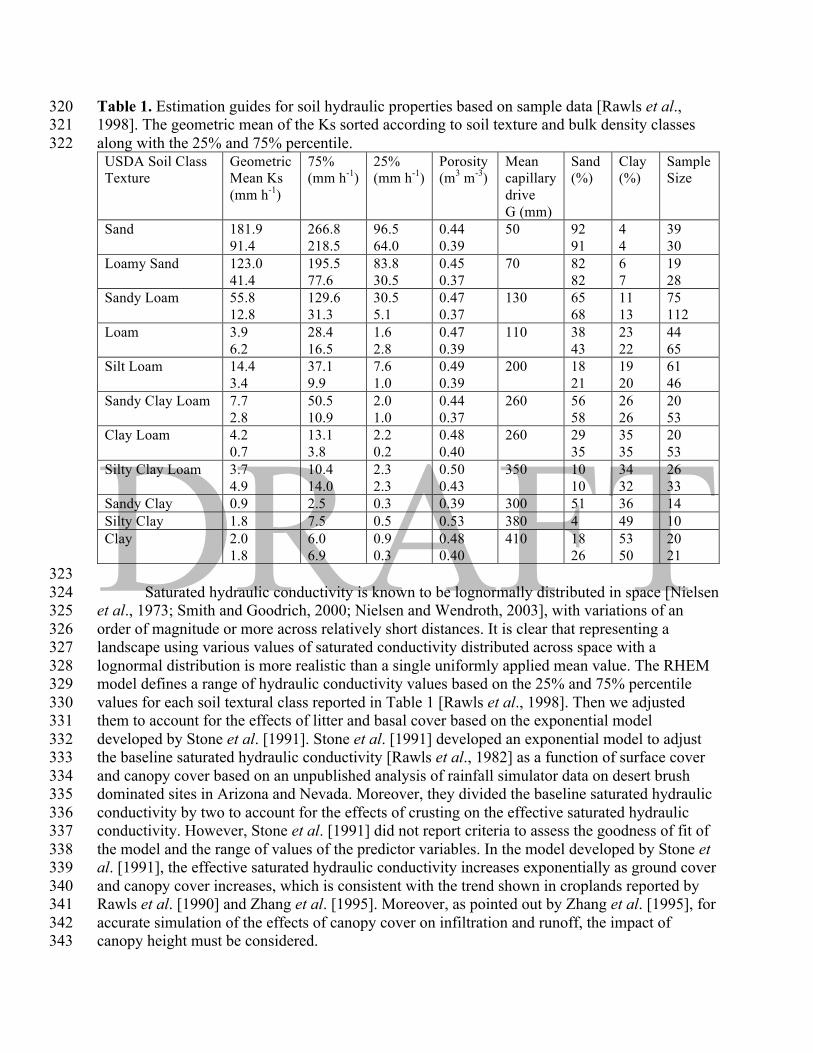
Table 1. Estimation guides for soil hydraulic properties based on sample data [Rawls et al., 320 1998]. The geometric mean of the Ks sorted according to soil texture and bulk density classes 321 along with the 25% and 75% percentile. 322
USDA Soil Class Texture
Geometric Mean Ks (mm h-1)
75% (mm h-1)
25% (mm h-1)
Porosity (m3 m-3)
Mean capillary drive G (mm)
Sand (%)
Clay (%)
Sample Size
Sand
181.9 91.4
266.8 218.5
96.5 64.0
0.44 0.39
50 92 91
4 4
39 30
Loamy Sand
123.0 41.4
195.5 77.6
83.8 30.5
0.45 0.37
70
82 82
6 7
19 28
Sandy Loam 55.8 12.8
129.6 31.3
30.5 5.1
0.47 0.37
130 65 68
11 13
75 112
Loam 3.9 6.2
28.4 16.5
1.6 2.8
0.47 0.39
110 38 43
23 22
44 65
Silt Loam 14.4 3.4
37.1 9.9
7.6 1.0
0.49 0.39
200 18 21
19 20
61 46
Sandy Clay Loam 7.7 2.8
50.5 10.9
2.0 1.0
0.44 0.37
260 56 58
26 26
20 53
Clay Loam 4.2 0.7
13.1 3.8
2.2 0.2
0.48 0.40
260 29 35
35 35
20 53
Silty Clay Loam 3.7 4.9
10.4 14.0
2.3 2.3
0.50 0.43
350 10 10
34 32
26 33
Sandy Clay 0.9 2.5 0.3 0.39 300 51 36 14 Silty Clay 1.8 7.5 0.5 0.53 380 4 49 10 Clay 2.0
1.8 6.0 6.9
0.9 0.3
0.48 0.40
410 18 26
53 50
20 21
323 Saturated hydraulic conductivity is known to be lognormally distributed in space [Nielsen 324
et al., 1973; Smith and Goodrich, 2000; Nielsen and Wendroth, 2003], with variations of an 325 order of magnitude or more across relatively short distances. It is clear that representing a 326 landscape using various values of saturated conductivity distributed across space with a 327 lognormal distribution is more realistic than a single uniformly applied mean value. The RHEM 328 model defines a range of hydraulic conductivity values based on the 25% and 75% percentile 329 values for each soil textural class reported in Table 1 [Rawls et al., 1998]. Then we adjusted 330 them to account for the effects of litter and basal cover based on the exponential model 331 developed by Stone et al. [1991]. Stone et al. [1991] developed an exponential model to adjust 332 the baseline saturated hydraulic conductivity [Rawls et al., 1982] as a function of surface cover 333 and canopy cover based on an unpublished analysis of rainfall simulator data on desert brush 334 dominated sites in Arizona and Nevada. Moreover, they divided the baseline saturated hydraulic 335 conductivity by two to account for the effects of crusting on the effective saturated hydraulic 336 conductivity. However, Stone et al. [1991] did not report criteria to assess the goodness of fit of 337 the model and the range of values of the predictor variables. In the model developed by Stone et 338 al. [1991], the effective saturated hydraulic conductivity increases exponentially as ground cover 339 and canopy cover increases, which is consistent with the trend shown in croplands reported by 340 Rawls et al. [1990] and Zhang et al. [1995]. Moreover, as pointed out by Zhang et al. [1995], for 341 accurate simulation of the effects of canopy cover on infiltration and runoff, the impact of 342 canopy height must be considered. 343
344 RHEM estimates of effective saturated hydraulic conductivity are computed as follows: 345
346 𝐾=l = 𝐾ml 𝑒
nl oE44=JpmdHdo (17) 347 348
In this equation, Kbi is the 25% percentile saturated hydraulic conductivity for each soil 349 textural class, i, listed in Table 1. P is defined as the natural log of the ratio of the 75% to the 350 25% percentile values of saturated hydraulic conductivity; litter is litter cover (%); and basal is 351 basal area cover (%). 352 353 2.2.2. Hydraulic roughness coefficient 354 355
Al-Hamdan et al. [2013] developed empirical equations that predict the total measured 356 friction factor (ft) by regressing the total measured friction against the measured vegetation and 357 rock cover, slope, and flow rate. The data used in their study were obtained from rangeland 358 rainfall simulator experiments conducted by the USDA-ARS Northwest Watershed Research 359 Center in Boise, Idaho. The data were collected from rangeland sites within the U.S. Great Basin 360 region and a broad range of slope angles (5.6% to 65.8%), soil types, and vegetation cover. 361 Many of these sites show some degree of disturbance and/or treatment, such as tree 362 encroachment, prescribed fire, wildfire, tree mastication, and/or tree cutting. Average slope, 363 canopy and ground cover, and micro-topography were measured for each plot [Pierson et al., 364 2007, 2009, 2010]. 365 366
According to Al-Hamdan et al. [2013], total hydraulic friction was negatively correlated 367 with flow discharge and the percentage of bare ground, and it was positively correlated with the 368 presence of vegetation cover and slope. Equations that were developed from concentrated flow 369 data have significantly different coefficients values compared to those obtained from sheet flow 370 data. The flow discharge and slope in the total friction equation enhanced the prediction of the 371 total friction, and consequently improved the estimation of the proportion of the assumed soil 372 friction to total friction. All equations derived by Al-Hamdan et al. [2013] showed that basal 373 plant cover was the most important effect on total friction among other cover attributes. 374 375
RHEM computes the total friction (ft) factor estimated by [Al-Hamdan et al., 2013] as 376 follows: 377 378 log 𝑓4 = −0.109 + 1.425 𝑙𝑖𝑡𝑡𝑒𝑟 + 0.442 𝑟𝑜𝑐𝑘 + 1.764 𝑏𝑎𝑠𝑎𝑙 + 𝑐𝑟𝑦𝑝𝑡𝑜𝑔𝑎𝑚𝑠 +379 2.068 𝑆 (18) 380 381 where litter is the fraction of area covered by litter to total area (m2 m-2), basal + cryptogams is 382 the fraction of area covered by basal plants and cryptogams to total area (m2 m-2), and rock is the 383 fraction of area covered by rock to total area (m2 m-2), and S is the slope (m m-1). 384 385 2.2.3. Splash and sheet erodibility factor 386 387
The RHEM model parameterization represents erosion processes on undisturbed 388 rangelands, as well as rangelands that show disturbances such as fire or woody plant 389
encroachment [Nearing et al., 2012; Hernandez et al. 2013; Al-Hamdan et al. 2016; Williams et 390 al. 2016]. In RHEM, soil detachment is predicted as a combination of two erosion processes, rain 391 splash and thin sheet flow (splash and sheet) detachment and concentrated flow detachment. 392 393
This section presents empirical equations developed by Al-Hamdan et al. [2016] using 394 piecewise regression analysis to predict erodibility across a broad range of soil texture classes 395 based on vegetation cover and surface slope steepness. 396 397 Bunch Grass: 398 399 Log5R 𝐾𝑠𝑠 =
4.154 − 2.547 ∗ 𝐺 − 0.7822 ∗ 𝐹 + 2.5535 ∗ 𝑆 if 𝐺 ≤ 0.475 3.1726975 − 0.4811 ∗ 𝐺 − 0.7822 ∗ 𝐹 + 2.5535 ∗ 𝑆 if 𝐺 > 0.475 (19) 400
401 Sod Grass: 402 403 Log5R 𝐾𝑠𝑠 =
4.2169 − 2.547 ∗ 𝐺 − 0.7822 ∗ 𝐹 + 2.5535 ∗ 𝑆 if 𝐺 ≤ 0.475 3.2355975 − 0.4811 ∗ 𝐺 − 0.7822 ∗ 𝐹 + 2.5535 ∗ 𝑆 if 𝐺 > 0.475 (20) 405
404 Shrub: 406 407 Log5R 𝐾𝑠𝑠 =
4.2587 − 2.547 ∗ 𝐺 − 0.7822 ∗ 𝐹 + 2.5535 ∗ 𝑆 if 𝐺 ≤ 0.475 3.2773975 − 0.4811 ∗ 𝐺 − 0.7822 ∗ 𝐹 + 2.5535 ∗ 𝑆 if 𝐺 > 0.475 (21) 409
408 Forbs: 410 411 Log5R 𝐾𝑠𝑠 =
4.1106 − 2.547 ∗ 𝐺 − 0.7822 ∗ 𝐹 + 2.5535 ∗ 𝑆 if 𝐺 ≤ 0.475 3.1292975 − 0.4811 ∗ 𝐺 − 0.7822 ∗ 𝐹 + 2.5535 ∗ 𝑆 if 𝐺 > 0.475 (22) 412
413 414 where G is the area fraction of ground cover, F is the area fraction of foliar cover, and S is the 415 slope gradient (expressed as a fraction). 416 417
The performance of the model with the new parameterization schemes indicates that 418 using Kss alone, as the indicator of erodibility factor in RHEM, works reasonably well as long as 419 concentrated flow paths work primarily as the transport tool of the splash and sheet-generated 420 sediments. The default value for Kw was set as 7.7x10⁻⁶ (s2 m-2) in the current RHEM V2.3. This 421 small value of concentrated flow erodibility is typical for undisturbed rangeland. It is 422 recommended to use the Kss equation that represents the dominant vegetation community in the 423 site to be evaluated. However, if the site does not have a dominant vegetation form or more 424 details are needed, then weight averaging between equations (19) through (22) based on the 425 percentage of life form would be used. Only in the special case of abrupt disturbance with steep 426 slopes (> 20%) and high silt, would the parameterization of Kw (as described in Section 2.2.4) be 427 needed. 428 429 2.2.4. Concentrated flow erodibility coefficients 430 431
The model employs two empirical functions developed by Al-Hamdan et al. (2012b) to 432 calculate Kw for a broad range of undisturbed rangeland sites and tree encroached sites. 433
434 𝑙𝑜𝑔5R 𝐾\ = −4.14 − 1.28𝑙𝑖𝑡𝑡𝑒𝑟 − 0.98𝑟𝑜𝑐𝑘 − 15.16𝑐𝑙𝑎𝑦 + 7.09𝑠𝑖𝑙𝑡 (23) 435 436 𝑙𝑜𝑔5R 𝐾\ = −4.05 − 0.81 𝑙𝑖𝑡𝑡𝑒𝑟 + 𝑐𝑟𝑦𝑝𝑡𝑜𝑔𝑎𝑚𝑠 + 𝑏𝑎𝑠𝑎𝑙 − 11.87𝑐𝑙𝑎𝑦437
+ 5.19𝑠𝑖𝑙𝑡 (24) 438 439 The model also has the capacity, as an option, to use equations developed by Al-Hamdan 440
et al. [2012b] for predicting maximum erodibility for a wide range of burned rangeland sites 441 including burned tree encroached sites. 442
443 𝑙𝑜𝑔5R 𝐾\ ��� dfg444
= −3.28 − 1.77𝑙𝑖𝑡𝑡𝑒𝑟 − 1.26𝑟𝑜𝑐𝑘 − 2.46 𝑏𝑎𝑠𝑎𝑙 + 𝑐𝑟𝑦𝑝𝑡𝑜445 + 3.53𝑠𝑖𝑙𝑡 25 446
447 𝑙𝑜𝑔5R 𝐾\ ��� dfg448
= −3.64 − 1.97 𝑙𝑖𝑡𝑡𝑒𝑟 + 𝑏𝑎𝑠𝑎𝑙 + 𝑐𝑟𝑦𝑝𝑡𝑜 − 1.85𝑟𝑜𝑐𝑘 − 4.99𝑐𝑙𝑎𝑦449 + 6.0𝑠𝑖𝑙𝑡 (26) 450
451 where litter, basal, and crypto are the fraction of area covered by litter, basal, and cryptogam to 452 total area (m2 m-2), rock is the fraction of area covered by rock to the total area (m2 m-2), and clay 453 and silt fraction. 454 455 2.3. PEST model parameterization 456 457 This study employs PEST software [Doherty, 2005] to calibrate RHEM parameters and 458 evaluate model performance for the 23 rainfall-runoff-erosion events at LH106. The parameter 459 calibration process included two approaches: first, the overland flow related parameters were 460 calibrated (effective saturated hydraulic conductivity, total friction factor, capillary drive, and 461 saturation). The parameters slope, coefficient of variation for Ke, and Interception were held 462 constant during the calibration. A detailed description of the overland flow parameters can be 463 found in Smith et al. [1995]; second, the calibration of the splash-and-sheet soil erodibility 464 coefficient was achieved by keeping constant the optimized overland flow parameters. 465 466 467 468 2.4. Statistical analysis 469 470 Nash-Sutcliffe Efficiency (NSE) [Nash and Sutcliffe, 1970] between observed and 471 calculated cumulative flows was calculated for each single event at LH106 as follows: 472 473
𝑁𝑆𝐸 = 1 −𝑂4 − 𝑀4
6�4�5
𝑂4 − 𝑂 6�4�5
(27) 474
475
where Ot, 𝑂 and Mt are observed cumulative flows at time step t, average cumulative value, and 476 modeled cumulative flows at time step t, respectively. T is the total number of time steps in the 477 simulation for each rainfall event. 478 479
Moreover, percent bias (PBIAS) [Gupta et al., 1999] and the RMSE-observations 480 standard deviation ratio (RSR) [Moriasi et. al., 2007] were calculated to evaluate the overall 481 performance of the model for runoff volume, peak runoff, and sediment yield estimates from the 482 23 events at LH106. 483
484 PBIAS was calculated by 485 486
𝑃𝐵𝐼𝐴𝑆 = 𝑂E − 𝑀E ∗ 100�
E�5
𝑂E�E�5
(28) 487
RSR was calculated by 488 489
𝑅𝑆𝑅 =𝑂E − 𝑀E
6�E�5
𝑂E − 𝑂 6�E�5
(29) 490
491 where Oi is the observed value of event i; Mi is the model generated value for the corresponding 492 event i; 𝑂 is the average of the observed values, and N is the total number of events at LH106. 493 494 495 3. Study Area and NRI database 496 497 3.1. Lucky Hills 106 watershed 498 499
The data used for the calibration and evaluation of the model were obtained from the 500 USDA-ARS Southwest Watershed Research Center's Lucky Hills experimental site, located in 501 the Walnut Gulch Experimental Watershed (WGEW). The semiarid WGEW is located in 502 southeastern Arizona (31o 43’N, 110o 41’W) and surrounds the town of Tombstone, Arizona 503 (Fig. 1). It has a mean annual temperature of 17.7oC and a mean annual precipitation of 350 mm, 504 the majority of which is a result of high-intensity convective thunderstorms in the summer 505 monsoon season [Keefer et al., 2015]. 506 507
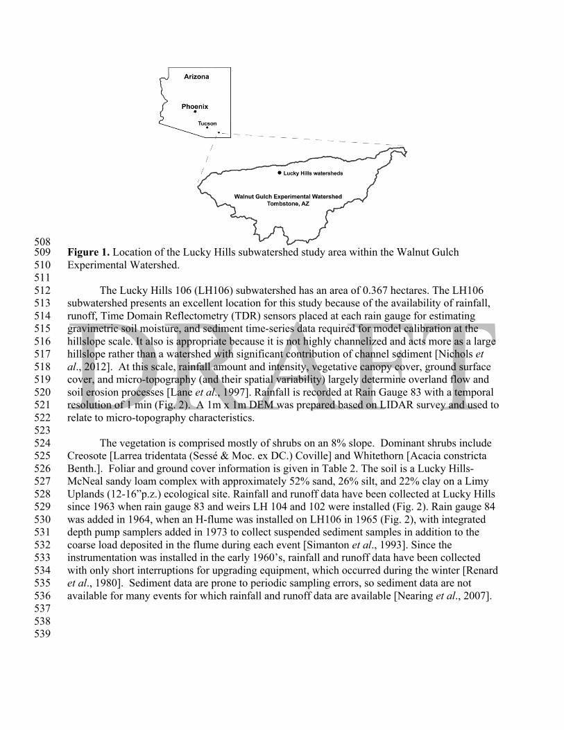
508 Figure 1. Location of the Lucky Hills subwatershed study area within the Walnut Gulch 509 Experimental Watershed. 510
511 The Lucky Hills 106 (LH106) subwatershed has an area of 0.367 hectares. The LH106 512
subwatershed presents an excellent location for this study because of the availability of rainfall, 513 runoff, Time Domain Reflectometry (TDR) sensors placed at each rain gauge for estimating 514 gravimetric soil moisture, and sediment time-series data required for model calibration at the 515 hillslope scale. It also is appropriate because it is not highly channelized and acts more as a large 516 hillslope rather than a watershed with significant contribution of channel sediment [Nichols et 517 al., 2012]. At this scale, rainfall amount and intensity, vegetative canopy cover, ground surface 518 cover, and micro-topography (and their spatial variability) largely determine overland flow and 519 soil erosion processes [Lane et al., 1997]. Rainfall is recorded at Rain Gauge 83 with a temporal 520 resolution of 1 min (Fig. 2). A 1m x 1m DEM was prepared based on LIDAR survey and used to 521 relate to micro-topography characteristics. 522
523 The vegetation is comprised mostly of shrubs on an 8% slope. Dominant shrubs include 524
Creosote [Larrea tridentata (Sessé & Moc. ex DC.) Coville] and Whitethorn [Acacia constricta 525 Benth.]. Foliar and ground cover information is given in Table 2. The soil is a Lucky Hills-526 McNeal sandy loam complex with approximately 52% sand, 26% silt, and 22% clay on a Limy 527 Uplands (12-16”p.z.) ecological site. Rainfall and runoff data have been collected at Lucky Hills 528 since 1963 when rain gauge 83 and weirs LH 104 and 102 were installed (Fig. 2). Rain gauge 84 529 was added in 1964, when an H-flume was installed on LH106 in 1965 (Fig. 2), with integrated 530 depth pump samplers added in 1973 to collect suspended sediment samples in addition to the 531 coarse load deposited in the flume during each event [Simanton et al., 1993]. Since the 532 instrumentation was installed in the early 1960’s, rainfall and runoff data have been collected 533 with only short interruptions for upgrading equipment, which occurred during the winter [Renard 534 et al., 1980]. Sediment data are prone to periodic sampling errors, so sediment data are not 535 available for many events for which rainfall and runoff data are available [Nearing et al., 2007]. 536
537 538 539
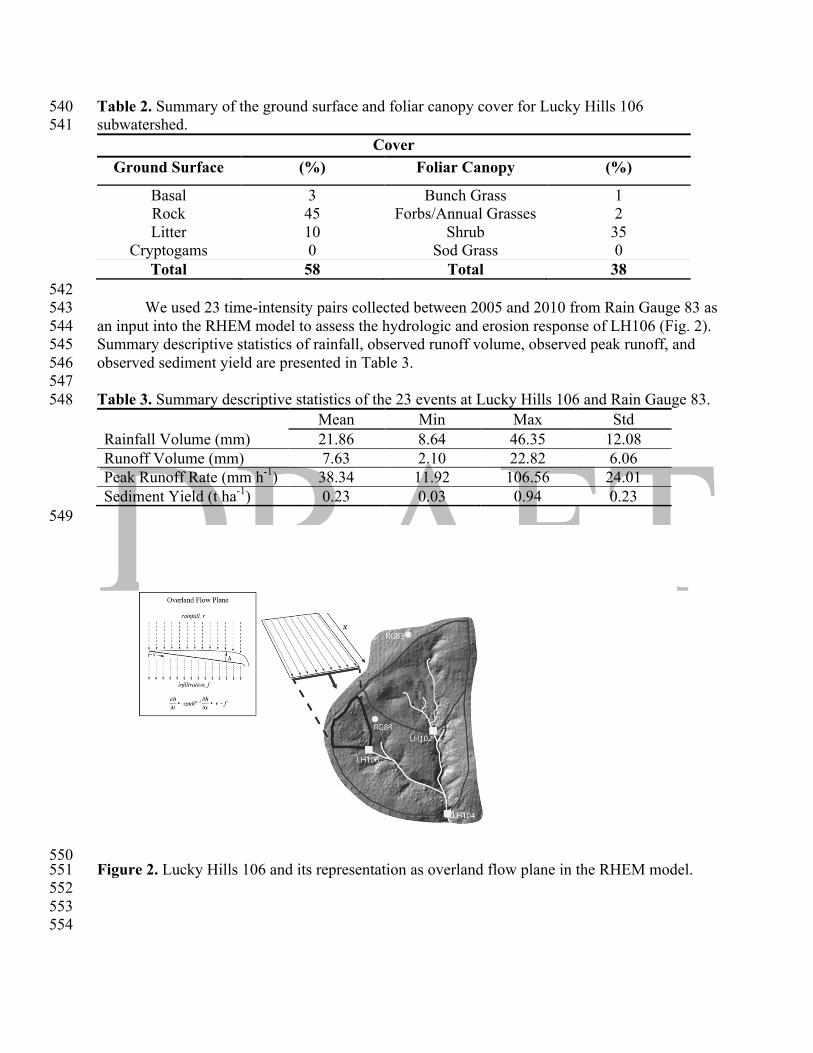
Table 2. Summary of the ground surface and foliar canopy cover for Lucky Hills 106 540 subwatershed. 541
Cover Ground Surface (%) Foliar Canopy (%)
Basal 3 Bunch Grass 1 Rock 45 Forbs/Annual Grasses 2 Litter 10 Shrub 35
Cryptogams 0 Sod Grass 0 Total 58 Total 38
542 We used 23 time-intensity pairs collected between 2005 and 2010 from Rain Gauge 83 as 543
an input into the RHEM model to assess the hydrologic and erosion response of LH106 (Fig. 2). 544 Summary descriptive statistics of rainfall, observed runoff volume, observed peak runoff, and 545 observed sediment yield are presented in Table 3. 546 547 Table 3. Summary descriptive statistics of the 23 events at Lucky Hills 106 and Rain Gauge 83. 548 Mean Min Max Std Rainfall Volume (mm) 21.86 8.64 46.35 12.08 Runoff Volume (mm) 7.63 2.10 22.82 6.06 Peak Runoff Rate (mm h-1) 38.34 11.92 106.56 24.01 Sediment Yield (t ha-1) 0.23 0.03 0.94 0.23
549
550 Figure 2. Lucky Hills 106 and its representation as overland flow plane in the RHEM model. 551 552 553
554
3.2. National Resources Inventory Field Measurements and Data Description 555 556
A major data source for rangeland assessment on non-federal lands is the National 557 Resource Inventory (NRI) [Goebel and Schmude, 1980]. The USDA-NRCS provided data for 558 542 NRI points collected between 2003 and 2014 across Arizona, New Mexico, and Utah to 559 parameterize the RHEM model. The points were grouped by soil texture classes, as follows: 560 sand, sandy loam, silt loam, and clay loam. For this study, we selected only the sandy loam soil 561 texture class to be in agreement with the LH106 soil texture class. We found 124 NRI points in 562 the sandy loam group. Furthermore, the 124 NRI data points were further grouped into annual 563 rainfall regimes measured at five weather stations. The Jornada weather station is located in New 564 Mexico, and Ganado, Laveen, Snowflake, and Willcox are in Arizona. 565
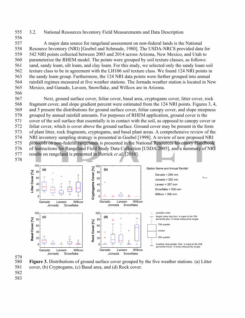
566 Next, ground surface cover, foliar cover, basal area, cryptogams cover, litter cover, rock 567
fragment cover, and slope gradient percent were estimated from the 124 NRI points. Figures 3, 4, 568 and 5 present the distributions for ground surface cover, foliar canopy cover, and slope steepness 569 grouped by annual rainfall amounts. For purposes of RHEM application, ground cover is the 570 cover of the soil surface that essentially is in contact with the soil, as opposed to canopy cover or 571 foliar cover, which is cover above the ground surface. Ground cover may be present in the form 572 of plant litter, rock fragments, cryptogams, and basal plant areas. A comprehensive review of the 573 NRI inventory sampling strategy is presented in Goebel [1998]. A review of new proposed NRI 574 protocols on non-federal rangelands is presented in the National Resources Inventory Handbook 575 of Instructions for Rangeland Field Study Data Collection [USDA 2005], and a summary of NRI 576 results on rangeland is presented in Herrick et al. [2010]. 577 578
579 Figure 3. Distributions of ground surface cover grouped by the five weather stations. (a) Litter 580 cover, (b) Cryptogams, (c) Basal area, and (d) Rock cover. 581 582 583
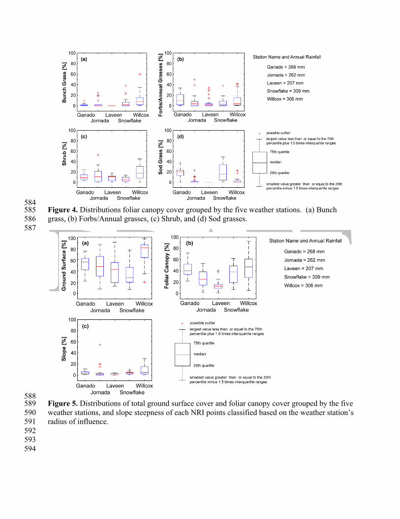
584 Figure 4. Distributions foliar canopy cover grouped by the five weather stations. (a) Bunch 585 grass, (b) Forbs/Annual grasses, (c) Shrub, and (d) Sod grasses. 586
587
588 Figure 5. Distributions of total ground surface cover and foliar canopy cover grouped by the five 589 weather stations, and slope steepness of each NRI points classified based on the weather station’s 590 radius of influence. 591 592 593 594

4. Results and Discussion 595 596
597 4.1. Model performance with RHEM parameter estimation equations 598
599 Total friction factor (ft), effective saturated hydraulic conductivity (Ke), splash and sheet 600
erodibility coefficient (Kss), and concentrated flow erodibility coefficient (Kw) were estimated 601 with the RHEM empirical equations for LH106 (Table 4). In this case we calculated Kw as the 602 geometric mean of Equations (23) and (24). 603
604 Table 4. RHEM parameter values estimated using the empirical equations. 605
Parameters Symbol Units Value Total friction factor ft dimensionless 5.50 Effective saturated hydraulic conductivity Ke (mm h-1) 7.29 Splash and sheet erodibility coefficient Kss dimensionless 2661.22 Concentrated flow erodibility coefficient Kw (s2 m-2) 8.62x10⁻⁶
606 The model performance based on the PBIAS and RSR goodness of fit criteria for runoff 607
volume, peak runoff, and sediment yield at LH106 is shown in Table 5. 608 609
Table 5. Model performance statistics for Lucky Hills 106. 610 Evaluation criteria Runoff Volume Peak Runoff Sediment Yield PBIAS (%) 2 21 -28 RSR (dimensionless) 0.49 0.57 0.58
611 Based on the model performance criteria reported by Moriasi et al. [2007], model 612
performance based on the RSR criterion can be evaluated as “very good” if 0 ≤ RSR ≤ 0.5 and 613 “good” if 0.50 < RSR ≤ 0.60. Therefore, these rankings suggest that RHEM performance can be 614 evaluated as “very good” for runoff volume, and “good” for peak runoff and sediment yield. 615 However, based on Moriasi et al., (2007) PBIAS criterion, the RHEM performance can be 616 evaluated for runoff volume and peak runoff as “very good’ if PBIAS < ±10, “good” if ±10 ≤ 617 PBIAS ≤ 15, and “satisfactory if ±15 ≤ PBIAS ≤ 25, and for sediment yield can be evaluated as 618 “good” if ±15 ≤ PBIAS ≤ 30. These criteria suggest that RHEM can be evaluated as ‘very good’ 619 for runoff volume, “satisfactory” for peak runoff, and “good” for sediment yield. 620
621 Positive PBIAS values indicate model underestimation bias, and negative values indicate 622
overestimation bias [Gupta et al., 1999]. It is apparent from Figure 6(a) that the model 623 performance for runoff volume prediction is poor with small events and improves with large 624 events, which is common for models [Nearing, 2000]. Figure 6(b) shows strong under prediction 625 of peak runoff among 14 runoff events, whereas sediment yield is in general over predicted for 626 the small events in Figure 6(c). One explanation for this behavior could be attributed to Kw; that 627 is, it was estimated by calculating the geometric mean between the equations (23) and (24) 628 developed by Al-Hamdan et al., [2012b]. Equation (23) estimates Kw as a function of litter, rock, 629 clay and silt, and Equation (24) based on litter, basal, clay, and silt. Al-Hamdan et al. [2012b] 630 proposed these equations to estimate average erodibility for a wide range of undisturbed 631
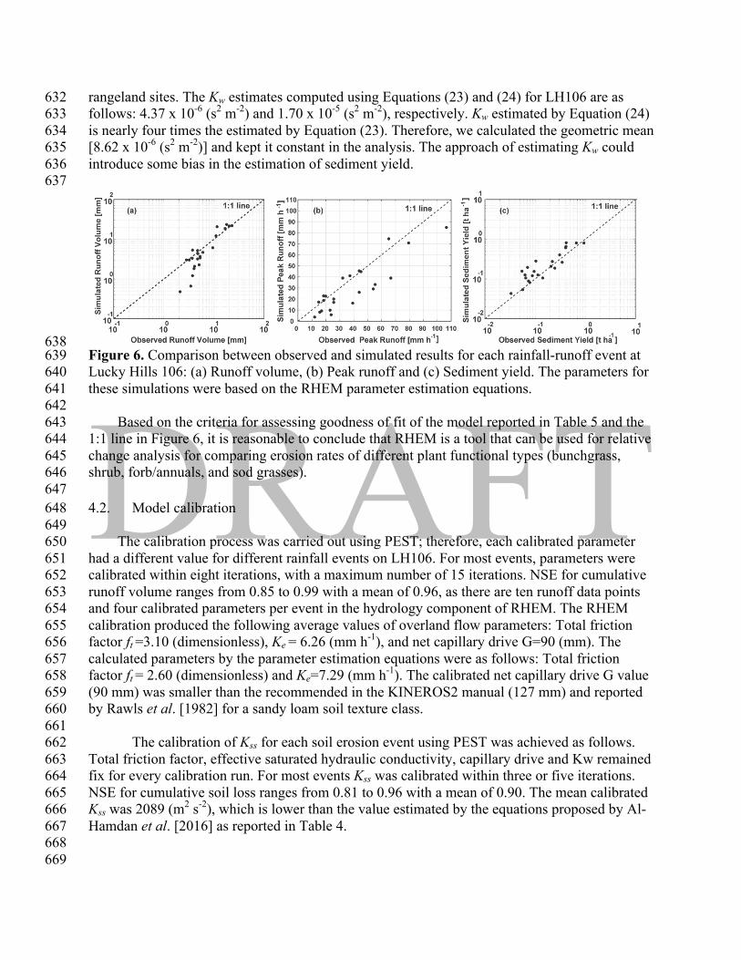
rangeland sites. The Kw estimates computed using Equations (23) and (24) for LH106 are as 632 follows: 4.37 x 10⁻⁶ (s2 m-2) and 1.70 x 10⁻⁵ (s2 m-2), respectively. Kw estimated by Equation (24) 633 is nearly four times the estimated by Equation (23). Therefore, we calculated the geometric mean 634 [8.62 x 10⁻⁶ (s2 m-2)] and kept it constant in the analysis. The approach of estimating Kw could 635 introduce some bias in the estimation of sediment yield. 636 637
638 Figure 6. Comparison between observed and simulated results for each rainfall-runoff event at 639 Lucky Hills 106: (a) Runoff volume, (b) Peak runoff and (c) Sediment yield. The parameters for 640 these simulations were based on the RHEM parameter estimation equations. 641 642
Based on the criteria for assessing goodness of fit of the model reported in Table 5 and the 643 1:1 line in Figure 6, it is reasonable to conclude that RHEM is a tool that can be used for relative 644 change analysis for comparing erosion rates of different plant functional types (bunchgrass, 645 shrub, forb/annuals, and sod grasses). 646 647 4.2. Model calibration 648 649
The calibration process was carried out using PEST; therefore, each calibrated parameter 650 had a different value for different rainfall events on LH106. For most events, parameters were 651 calibrated within eight iterations, with a maximum number of 15 iterations. NSE for cumulative 652 runoff volume ranges from 0.85 to 0.99 with a mean of 0.96, as there are ten runoff data points 653 and four calibrated parameters per event in the hydrology component of RHEM. The RHEM 654 calibration produced the following average values of overland flow parameters: Total friction 655 factor ft =3.10 (dimensionless), Ke = 6.26 (mm h-1), and net capillary drive G=90 (mm). The 656 calculated parameters by the parameter estimation equations were as follows: Total friction 657 factor ft = 2.60 (dimensionless) and Ke=7.29 (mm h-1). The calibrated net capillary drive G value 658 (90 mm) was smaller than the recommended in the KINEROS2 manual (127 mm) and reported 659 by Rawls et al. [1982] for a sandy loam soil texture class. 660
661 The calibration of Kss for each soil erosion event using PEST was achieved as follows. 662
Total friction factor, effective saturated hydraulic conductivity, capillary drive and Kw remained 663 fix for every calibration run. For most events Kss was calibrated within three or five iterations. 664 NSE for cumulative soil loss ranges from 0.81 to 0.96 with a mean of 0.90. The mean calibrated 665 Kss was 2089 (m2 s-2), which is lower than the value estimated by the equations proposed by Al-666 Hamdan et al. [2016] as reported in Table 4. 667
668 669
4.3 Model Evaluation using NRI data 670 671
This section reports the effects of ground cover on total friction factor (ft), effective 672 saturated hydraulic conductivity (Ke), and splash and sheet erodibility factor (Kss) estimated 673 using the parameter estimation equations. 674
675 To investigate the effect of foliar canopy cover and ground cover on sediment yield on the 676
124 NRI points, the RHEM model was run for a 300-year synthetic rainfall sequence generated 677 by CLIGEN V5.3 [Nicks et al., 1995] based on the statistics of historic rainfall at each climate 678 station. 679 680
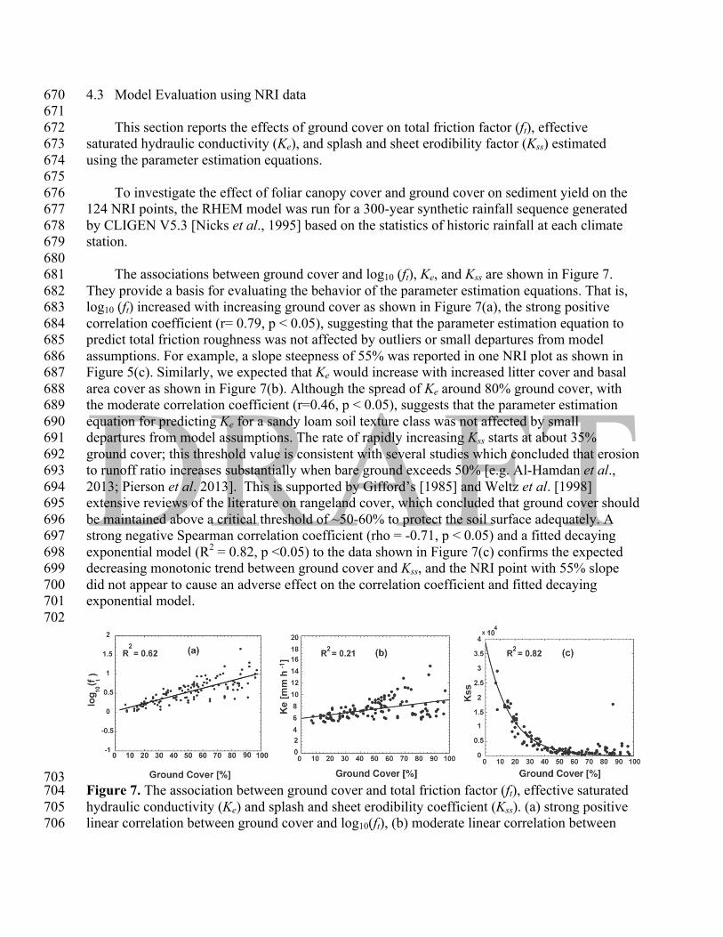
The associations between ground cover and log10 (ft), Ke, and Kss are shown in Figure 7. 681 They provide a basis for evaluating the behavior of the parameter estimation equations. That is, 682 log10 (ft) increased with increasing ground cover as shown in Figure 7(a), the strong positive 683 correlation coefficient (r= 0.79, p < 0.05), suggesting that the parameter estimation equation to 684 predict total friction roughness was not affected by outliers or small departures from model 685 assumptions. For example, a slope steepness of 55% was reported in one NRI plot as shown in 686 Figure 5(c). Similarly, we expected that Ke would increase with increased litter cover and basal 687 area cover as shown in Figure 7(b). Although the spread of Ke around 80% ground cover, with 688 the moderate correlation coefficient (r=0.46, p < 0.05), suggests that the parameter estimation 689 equation for predicting Ke for a sandy loam soil texture class was not affected by small 690 departures from model assumptions. The rate of rapidly increasing Kss starts at about 35% 691 ground cover; this threshold value is consistent with several studies which concluded that erosion 692 to runoff ratio increases substantially when bare ground exceeds 50% [e.g. Al-Hamdan et al., 693 2013; Pierson et al. 2013]. This is supported by Gifford’s [1985] and Weltz et al. [1998] 694 extensive reviews of the literature on rangeland cover, which concluded that ground cover should 695 be maintained above a critical threshold of ~50-60% to protect the soil surface adequately. A 696 strong negative Spearman correlation coefficient (rho = -0.71, p < 0.05) and a fitted decaying 697 exponential model (R2 = 0.82, p <0.05) to the data shown in Figure 7(c) confirms the expected 698 decreasing monotonic trend between ground cover and Kss, and the NRI point with 55% slope 699 did not appear to cause an adverse effect on the correlation coefficient and fitted decaying 700 exponential model. 701 702
703 Figure 7. The association between ground cover and total friction factor (ft), effective saturated 704 hydraulic conductivity (Ke) and splash and sheet erodibility coefficient (Kss). (a) strong positive 705 linear correlation between ground cover and log10(ft), (b) moderate linear correlation between 706
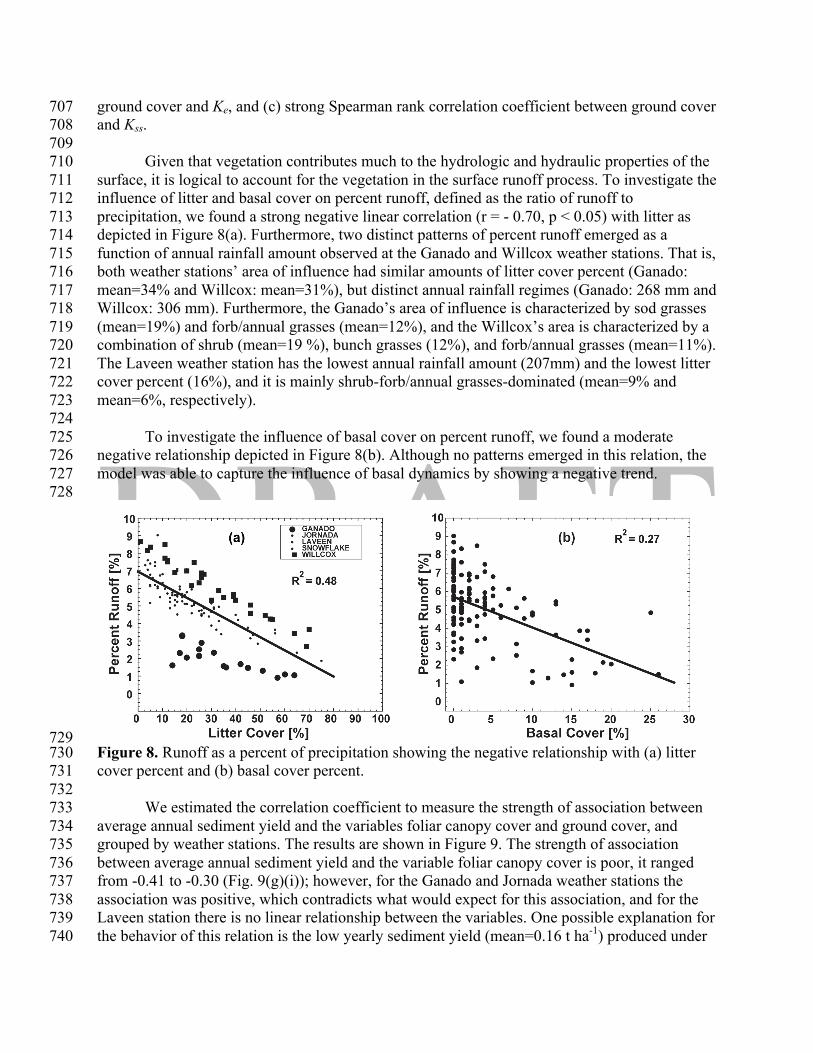
ground cover and Ke, and (c) strong Spearman rank correlation coefficient between ground cover 707 and Kss. 708 709 Given that vegetation contributes much to the hydrologic and hydraulic properties of the 710 surface, it is logical to account for the vegetation in the surface runoff process. To investigate the 711 influence of litter and basal cover on percent runoff, defined as the ratio of runoff to 712 precipitation, we found a strong negative linear correlation (r = - 0.70, p < 0.05) with litter as 713 depicted in Figure 8(a). Furthermore, two distinct patterns of percent runoff emerged as a 714 function of annual rainfall amount observed at the Ganado and Willcox weather stations. That is, 715 both weather stations’ area of influence had similar amounts of litter cover percent (Ganado: 716 mean=34% and Willcox: mean=31%), but distinct annual rainfall regimes (Ganado: 268 mm and 717 Willcox: 306 mm). Furthermore, the Ganado’s area of influence is characterized by sod grasses 718 (mean=19%) and forb/annual grasses (mean=12%), and the Willcox’s area is characterized by a 719 combination of shrub (mean=19 %), bunch grasses (12%), and forb/annual grasses (mean=11%). 720 The Laveen weather station has the lowest annual rainfall amount (207mm) and the lowest litter 721 cover percent (16%), and it is mainly shrub-forb/annual grasses-dominated (mean=9% and 722 mean=6%, respectively). 723 724 To investigate the influence of basal cover on percent runoff, we found a moderate 725 negative relationship depicted in Figure 8(b). Although no patterns emerged in this relation, the 726 model was able to capture the influence of basal dynamics by showing a negative trend. 727 728
729 Figure 8. Runoff as a percent of precipitation showing the negative relationship with (a) litter 730 cover percent and (b) basal cover percent. 731 732
We estimated the correlation coefficient to measure the strength of association between 733 average annual sediment yield and the variables foliar canopy cover and ground cover, and 734 grouped by weather stations. The results are shown in Figure 9. The strength of association 735 between average annual sediment yield and the variable foliar canopy cover is poor, it ranged 736 from -0.41 to -0.30 (Fig. 9(g)(i)); however, for the Ganado and Jornada weather stations the 737 association was positive, which contradicts what would expect for this association, and for the 738 Laveen station there is no linear relationship between the variables. One possible explanation for 739 the behavior of this relation is the low yearly sediment yield (mean=0.16 t ha-1) produced under 740
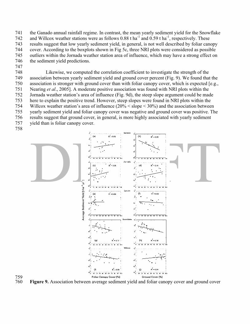
the Ganado annual rainfall regime. In contrast, the mean yearly sediment yield for the Snowflake 741 and Willcox weather stations were as follows 0.88 t ha-1 and 0.59 t ha-1, respectively. These 742 results suggest that low yearly sediment yield, in general, is not well described by foliar canopy 743 cover. According to the boxplots shown in Fig 5c, three NRI plots were considered as possible 744 outliers within the Jornada weather station area of influence, which may have a strong effect on 745 the sediment yield predictions. 746
747 Likewise, we computed the correlation coefficient to investigate the strength of the 748
association between yearly sediment yield and ground cover percent (Fig. 9). We found that the 749 association is stronger with ground cover than with foliar canopy cover, which is expected [e.g., 750 Nearing et al., 2005]. A moderate positive association was found with NRI plots within the 751 Jornada weather station’s area of influence (Fig. 9d), the steep slope argument could be made 752 here to explain the positive trend. However, steep slopes were found in NRI plots within the 753 Willcox weather station’s area of influence (20% < slope < 30%) and the association between 754 yearly sediment yield and foliar canopy cover was negative and ground cover was positive. The 755 results suggest that ground cover, in general, is more highly associated with yearly sediment 756 yield than is foliar canopy cover. 757
758
759 Figure 9. Association between average sediment yield and foliar canopy cover and ground cover 760
5. Conclusions 761 762
Reliable parameter inference is critical for meaningful prediction of soil erosion models. 763 The capability of RHEM for simulating flow and soil erosion was tested on a small watershed in 764 Arizona and on 124 NRI plots placed in Arizona and New Mexico. In particular, we were 765 interested in evaluating the parameter estimation equations for predicting total friction factor (ft), 766 effective saturated hydraulic conductivity (Ke), splash and sheet erodibility coefficient (Kss), and 767 concentrated flow erodibility coefficient (Kw). 768
769 The performance of the model for predicting runoff volume, peak runoff, and sediment 770
yield using the parameter estimation equations in 23 events at LH106 is as follows. Based on the 771 RSR criterion [Moriasi et al., 2007], model performance is “very good” for runoff volume, and 772 “good” for peak runoff and sediment yield. However, based on the PBIAS criterion [Moriasi et 773 al., 2007], the performance of the model can be evaluated as ‘very good’ for runoff volume, 774 “satisfactory” for peak runoff, and “good” for sediment yield. We achieved acceptable goodness 775 of fit for runoff volume and sediment yield in the model calibration at LH106 on 23 events, the 776 level of calibration was quantified with the Nash and Sutcliffe efficiency coefficient. 777
778 We compared the parameters calculated by the parameter estimation equations with the 779
calibrated parameters at LH106. The parameter values calculated with the parameter estimation 780 equations fell within the lowest and highest calibrated values of each parameter. The ability of 781 the parameter estimation equations to adequately produce parameter values for the application of 782 RHEM on a small watershed suggest that the model is well suited for small subwatersheds, 783 provided that gully erosion is not the main active process in the watershed. 784
785 It should be noted that we kept Kw (8.62 x 10⁻⁶ m2 s-2) constant to avoid over-786
parameterization and cause adverse effects on model soil erosion predictive capacity. Runoff 787 generation and sediment predictions are simulated in the model with separate functions, but we 788 assumed that splash and sheet and detachment by concentrated flow are processes acting 789 simultaneously in rangelands. Therefore, particular attention is needed as to whether Kw remains 790 constant in further applications of RHEM outside of Lucky Hills environment. 791
792 We selected 124 NRI points in Arizona and New Mexico and ran those points through 793
RHEM to estimate runoff and sediment yield. The NRI points were placed into five groups 794 according to the weather station’s area of influence. The results suggest that the parameter 795 estimation equations conveyed coherent information to the model. That is, moderate and strong 796 negative correlation coefficients between ground cover percent and total friction factor, effective 797 hydraulic conductivity, and splash and sheet erodibility coefficient were achieved. Likewise, 798 moderate and strong negative correlation coefficients were found between litter cover and basal 799 cover percent and percent runoff. In contrast, weak and moderate negative correlation 800 coefficients were found between foliar canopy cover and ground cover and sediment yield, in the 801 Jornada weather station group, the correlation coefficient was weak and positive. Lack of 802 information on this location prevents further analysis as to explain the behavior of the weak 803 positive trend between the foliar canopy and ground cover variables and sediment yield. We 804 noticed NRI points having large slopes (55 %) in this area and considered as possible outliers, 805
these inconsistencies in the data may be transferred and amplified in the sediment yield 806 simulations. 807
808 Evaluation of the model predictions undertaken in this study demonstrates that RHEM 809
produces results of satisfactory quality when simulating large flow and soil erosion events, but a 810 greater degree of uncertainty is associated with predictions of small runoff and soil erosion 811 events. 812
A high level of empirical knowledge and, in particular, prior knowledge of rangeland, 813 management practices, soil and climatic conditions is a big advantage during all phases of the 814 RHEM modeling, from hillslope characterization to interpretation of results. 815
816
References 817
818 Al-Hamdan O. Z, F. B. Pierson, M. A. Nearing, C. J. Williams, M. Hernandez, J. Boll, S. K. 819 Nouwakpo, M. A. Weltz, and K. E. Spaeth (2016), Developing a parameterization approach of 820 soil erodibility for the Rangeland Hydrology and Erosion Model (RHEM). Journal of the 821 American Society of Agricultural and Biological Engineers, (in press). 822 823 Al-Hamdan O. Z, F. B. Pierson, M. A. Nearing, J. J. Stone, C. J. Williams, C. A. Moffet, P. R. 824 Kormos, J. Boll, and M. A. Weltz (2012a), Characteristics of concentrated flow hydraulics for 825 rangeland ecosystems: implications for hydrologic modeling. Earth Surface Processes Landforms 826 37: 157–168. 827 828 Al-Hamdan, O. Z., F. B. Pierson, M. A. Nearing, C. J. Williams, J. J. Stone, P. R. Kormos, J. 829 Boll, and M. A. Weltz (2012b), Concentrated flow erodibility for physically based erosion 830 models: Temporal variability in disturbed and undisturbed rangelands. Water Resources 831 Research. 48, W07504.l 832 833 Al-Hamdan, O., F. B. Pierson, M. A. Nearing, C. J. Williams, J. J. Stone, P. R. Kormos, J. Boll, 834 M. A. Weltz (2013), Risk assessment of erosion from concentrated flow on rangelands using 835 overland flow distribution and shear stress partitioning. Transactions of the ASABE. 56(2):539-836 548. 837 838 Al-Hamdan, O.Z., M. Hernandez, F. B. Pierson, M. A. Nearing, C. J. Williams, J. J. Stone, J. 839 Boll, and M. A. Weltz (2014), Rangeland Hydrology and Erosion Model (RHEM) enhancements 840 for applications on disturbed rangelands. Hydological Processes. DOI: 10.1002/hyp.10167. 841 842 Bennett, J. P. (1974), Concepts of mathematical modeling of sediment yield. Water Resources 843 Research 10(3):485-492. 844 845 Briske, D.D., L. W. Jolley, L. F. Duriancik, and J. P. Dobrowolski (2011), Introduction to the 846 Conservation Effects Assessment Project and Rangeland Literature Syntheses. In: Conservation 847 Benefits of Rangeland Practices, USDA-NRCS. 848 849
Bulygina, N.S., M. A. Nearing, J. J. Stone, and M. H. Nichols (2007), DWEPP: A dynamic soil 850 erosion model based on WEPP source terms. Earth Surface Proceses and Landforms. 32:998-851 1012. 852 853 Cannon, S.H., Kirkham, R.M., Parise, M., 2001a. Wildfire-related debris flow initiation 854 processes, Storm King Mountain, Colorado. Geomorphology 39, 171 – 188. 855 856 Cerda`, A., 1998. Post-fire dynamics of erosional processes under Mediterranean climatic 857 conditions. Zeitschrift fu¨ r Geomorphologie 42, 373 – 398. 858 859 Dortignac, E. J. and L. D. Love, (1961) Infiltration studies on ponderosa pine ranges of 860 Colorado. Rocky Mountain Forest and Range Exp. Sta., Pap 59, 34p. 861 862 Fair, G. M., J. C. Geyer, and D. A. Okun, (1966) Water and Wastewater Engineering, Volume 1: 863 Water Supply and Wastewater Removal, John Wiley & Sons Inc.; 1St Edition. 864 865 Flanagan, D. C., and M. A. Nearing, eds. 1995. USDA Water Erosion Prediction Project 866 Hillslope Profile and Watershed Model Documentation. NSERL Report No. 10. West Lafayette, 867 Ind.: USDA-ARS National Soil Erosion Research Laboratory. 868 869 Foltz, R.B., H. Rhee and W.J. Elliot. 2008. Modeling changes in rill erodiblity and critical shear 870 stress on native surface roads. Hydrologic Processes 22:4783-4788. 871 872 Foster GR. 1982. Modeling the erosion process. In Hydrologic Modeling of Small Watersheds, 873 ASAE Monograph 5, Haan CT (ed.). ASAE: St. Joseph, MI; 297–360 874 875 Goebel, J.J., and K.O. Schmude. 1980. Planning the SCS national resource inventory. In Arid 876 Land Resource Inventories: Developing Cost-Efficient Methods. General Technical Report WO-877 28. U.S. Department of Agriculture, Forest Service, Washington, D.C. pp. 148-153. 878 879 Goebel, J. J. (1998) The National Resources Inventory and its role in U.S. agriculture, 880 Agricultural Statistics 2000, International Statistical Institute, Voorburg, The Netherlands, 181-881 192. 882 883 Green W. H. and A. G. Ampt (1911), Studies of soil physics, part I – the flow of air and water 884 through soils. Journal of Agricultural Science 4: 1–24. 885 886 IRWET and NRST, (1998), Interagency Rangeland Water Erosion Project report and state data 887 summaries. Interagency Rangeland Water Erosion Team (IRWET) and National Rangeland 888 Study Team (NRST). NWRC 98-‐1. Boise, Idaho: USDA-‐ARS Northwest Watershed Research 889 Center. 890 891 Kalin L, R. S. Govindaraju, and M. M. Hantush (2004), Development and application of a 892 methodology sediment source identification. 1: Modified unit sedimentograph approach. Journal 893 of Hydrologic Engineering, ASCE 9(3): 184–193 894 895
Lane, L.J., M. Hernandez, and M. H. Nichols (1997), Dominant processes controlling sediment 896 yield as functions of watershed scale. Proc. MODSIM 97, Internat'l. Conf. on Modelling and 897 Simulation, Dec. 8-11, Hobart, Tasmania, A.D. McDonald and M. McAleer (eds.), Vol. 1, 5 pp. 898 899 Havstad, K.M., Deb Peters, B. Allen-Diaz, B. T. Bestelmeyer, D. Briske, J. L. Brown, M. 900 Brunson, J. E. Herrick, P. Johnson, L. Joyce, R. Pieper, A. J. Svejcar, J. Yao, J. Bartolome, and 901 L. Huntsinger (2009), The western United States rangelands, a major resource. In: Grassland, 902 Quietness and Strength for a New American Agriculture, Chapter 5 903 904 Hernandez, M., M. A. Nearing, J. J. Stone, G. Armendariz, F. B. Pierson, O. Z. Al-Hamdan, C. 905 J. Williams, K. E. Spaeth, M. A. Weltz, H. Wei, P. Heilman, and D. C. Goodrich (2015), Web-906 Based Rangeland Hydrology and Erosion Model. Proceedings 907 908 Hernandez, M., M.A. Nearing, F.B. Pierson, C. J. Williams, K. E. Spaeth, and M. A. Weltz, 909 M.A. 2016. A risk-based vulnerability approach for rangeland management. In: Proceedings of 910 the 10th International Rangeland Congress, The Future Management of Grazing and Wild Lands 911 in a High Tech World, July 17-22, 2016, Saskatoon, SK, Canada. p. 1014-1015. 912 913 Hernandez, M., M. A. Nearing, J. J. Stone, F. B. Pierson Jr., H. Wei, K. E. Spaeth, P. Heilman, 914 M. A. Weltz, and D. C. Goodrich (2013), Application of a rangeland soil erosion model using 915 NRI data in southeastern Arizona. Journal of Soil and Water Conservation. 68(6):512-525. 916 917 Keefer, T.O., K. G. Renard, D. C. Goodrich, P. Heilman, and C. L. Unkrich (2015), Quantifying 918 Extreme Precipitation Events and their Hydrologic Response in Southeastern Arizona. Journal of 919 Hydrologic Engineering. 21(1): 1-10. 10.1061/(ASCE)HE.1943-5584.0001270. 920 921 Kustas, W.P. and D. C. Goodrich (1994), Preface for the Monsoon '90 multidisciplinary field 922 campaign. Water Resour. Res. 30(5):1211-1225. 923 Morris, S.E. and T. A. Moses (1987), Forest fire and the natural soil erosion regime in the 924 Colorado Front Range. Annals of the Association of American Geographers 77, 245 – 254. 925 926 Meeuwig, R. O. (1969), Infiltration and Soil Erosion as Influenced by Vegetation and Soil in 927 Northern Utha, Journal of Range Management, 23:185-189 928 929 Morris, S.E., and T. A. Moses, (1987) Forest fire and the natural soil erosion regime in the 930 Colorado Front Range. Annals of the Association of American Geographers 77, 245 – 254. 931 932 Nearing, M.A. 2000. Evaluating soil erosion models using measured plot data: Accounting for 933 variability in the data. Earth Surface Processes and Landforms. 25:1035-1043. 934 935 Nearing, M.A., V. Jetten, C. Baffaut, O. Cerdan, A. Couturier, M. Hernandez, Y. Le Bissonnais, 936 M.H. Nichols, J.P. Nunes, C.S. Renschler, V. Souchère, and K. van Oost. (2005), Modeling 937 response of soil erosion and runoff to changes in precipitation and cover. Catena 61(2-3):131–938 154. 939 940
Nearing, M.A., M. H. Nichols, J.J. Stone, K.G. Renard, and J.R. Simanton (2007), Sediment 941 yields from unit-source semi-arid watersheds at Walnut Gulch. Water Resources Research 942 43:W06426, doi:10.1029/2006WR005692. 943 944 Nearing, M.A. and P. B. Hairsine (2011), The Future of Soil Erosion Modelling. Ch. 20 In: 945 Morgan, R.P. and M.A. Nearing (eds.). 2011. Handbook of Erosion Modelling. ISBN: 978-1- 946 051-9010-7. 416 pgs. Wiley-Blackwell Publishers, Chichester, West Sussex, UK. pps. 391-397. 947 948 Nearing, M.A., H. Wei, J. J. Stone, F. B. Pierson, K. E. Spaeth, M. A. Weltz, D. C. Flanagan, 949 and M. Hernandez (2011) A Rangeland Hydrology and Erosion Model. Trans. American Society 950 Agricultural Engineers. 54(3): 901-908. 951 952 Nearing, M.A., F. F. Pruski, and M. R. O'Neal (2004), Expected climate change impacts on soil 953 erosion rates: A review. J. Soil and Water Cons. 59(1):43-50. 954 955 Nearing M. A., L. D. Norton, D. A. Bulgakov, G.A. Larionov, L. T. West, and K. M. Dontsova 956 (1997), Hydraulics and erosion in eroding rills. Water Resources Research 33: 865–876. 957 958 Nichols, M.H., M.A. Nearing, V.O. Polyakov, J.J. Stone (2012), A sediment budget for a small 959 semiarid watershed in southeastern Arizona, USA. Geomorphology 180: 137-145 DOI: 960 10.1016/j.geomorph.2012.10.002. 961 962 Parlange, J.Y., I. Lisle, R. D. Braddock, and R. E. Smith, (1982), "The three-parameter 963 infiltration equation." Soil Science, 133(6), pp337-341. 964 965 Pierson, F.B., D. H. Carlson, and K. E. Spaethe (2002), Impacts of wildfire on soil hydrological 966 properties of steep sagebrush-steppe rangeland. International Journal of Wildfire 11, 145 – 151. 967 968 Pierson, F. B., J. D. Bates, T. J. Svejcar, and S. P. Hardegree (2007), Runoff and erosion after 969 cutting western juniper, Rang. Ecology Manage., 60, 285–292. -- Highlighted Sep 6, 2016 970 971 Pierson, F.B., P. R. Robichaud, C. A. Moffet, K. E. Spaeth, S. P. Hardegree, P. E. Clark, and C. 972 J. Williams (2008), Fire effects on rangeland hydrology and erosion in a steep sagebrush-973 dominated landscape. Hydrological Processes 22, 2916–2929. 974 975 Pierson, F. B., C. A. Moffet, C. J. Williams, S. P. Hardegree, and P. Clark (2009), Prescribed-fire 976 effects on rill and interrill runoff and erosion in a mountainous sagebrush landscape, Earth Surf. 977 Processes Landforms, 34,193–203. 978 979 Pierson, F. B., C. J. Williams, P. R. Kormos, S. P. Hardegree, and P. E.Clark (2010), Hydrologic 980 vulnerability of sagebrush steppe following pinyon and juniper encroachment, Rang. Ecol. 981 Manage., 63, 614–629, doi:10.2111/REM-D-09-00148.1. -- Highlighted Sep 6, 2016. 982 983 Pierson, F.B., Carlson, D.H., Spaethe, K.E., 2002. Impacts of wildfire on soil hydrological 984 properties of steep sagebrush-steppe rangeland. International Journal of Wildfire 11, 145 – 151. 985 986
Rawls, W. J., D. L. Brakensiek, J. R. Simanton, and D. Kho, (1990), Development of a crust 987 factor for a Green Ampt model. Transactions of the ASAE 33(4):1224-1228 988 989 Rawls, W. J., D. L. Brakensiek and K. E. Saxton (1982) Estimation of Soil Water Properties, 990 Transactions of the ASAE, Paper No. 81-2510. 991 992 Rawls, W. L., D. Gimenez, and R. Grossman, (1998) Use of soil texture, bulk density, and slope 993 of the water retention curve to predict saturated hydraulic conductivity, Transactions of the 994 ASAE 41:983-988 995 996 Renard, K.G., M. H. Nichols, D. A. Woolhiser, and H. B. Osborn (2008) A brief background on 997 the U.S. Department of Agriculture Agricultural Research Service Walnut Gulch Experimental 998 Watershed. Water Resources Research. Vol. 44, W05S02 999 1000 Renard, K. G. (1993). “Agricultural impacts in an arid environment: Walnut Gulch case study.” 1001 Hydrol. Sci. Tech., 9(1–4), 145–190. 1002 1003 Renard, K.G. 1980. Estimating erosion and sediment yield from rangelands. Proc. ASCE Sym. 1004 on Watershed Manage. '80, Boise, ID, pp. 164-175. 1005 1006 Scott, D.F., Van Wyk, D.B., 1990. The effects of wildfire on soil wettability and hydrological 1007 behavior of an afforested catchment. Journal of Hydrology 121, 239 – 256. 1008 1009 Shakesby, R.A., Coelho, C. de O.A., Ferreira, A.D., Terry, J.P., Walsh, R.P.D., 1993. Wildfire 1010 impacts on soil erosion and hydrology in wet Mediterranean forest, Portugal. International 1011 Journal of Wildland Fire 3, 95 – 110 1012 1013 Simanton, J.R., W. R. Osterkamp, and K. G. Renard (1993), Sediment yield in a semiarid basin: 1014 Sampling equipment impacts. Proc. Yokohama, Japan Sym., Sediment Problems: Strategies for 1015 Monitoring, Prediction and Control, R.F. Hadley and T. Mizuyama (eds.), July, IAHS Pub. No. 1016 217, pp. 3-9. 1017 1018 Smith, R.E., D. C. Goodrich, D. A. Woolhiser, and C. L. Unkrich (1995). KINEROS - A 1019 kinematic runoff and erosion model. Chpt. 20 In: Computer Models of Watershed Hydrology, 1020 V.P. Singh (ed.), Water Resources Publs., pp. 697-732. 1021 1022 Smith, R. E., C. Corradini, and F. Melone (1993), Modeling infiltration for multi-storm runoff 1023 event. Water Resour. Res., 29 (1), 133-44. 1024 1025 Smith, R. E. and Parlange, J.- Y (1978). A parameter-efficient hydrologic infiltration model. 1026 Water Resour. Res., 14 (3), 533-8. 1027 1028 Spaeth, K. E., F. B. Pierson, M. A. Weltz, and J. B. Awang, (1996), Gradient analysis of 1029 infiltration and environmental variables as related to rangeland vegetation. Trans. ASAE 39(1): 1030 67-‐77. 1031 1032
Stone, J.J., L. J. Lane, and E. D. Shirley (1992), Infiltration and runoff simulation on a plane. 1033 Trans. ASAE 35(1):161-170. 1034 1035 Tromble, J. M., K. G. Renard and A.P. Thatcher, (1973) Infiltration for Three Rangeland Soil-1036 Vegetation Complexes, Journal of Range Management, 27(4). 1037 1038 Wei, H., M. A. Nearing, J. J. Stone, D. P. Guertin, K. E. Spaeth, F. B. Pierson, M. H. Nichols, C. 1039 A. Moffett (2009), A new Splash and Sheet Erosion Equation for Rangelands. Soil Science of 1040 America Journal. 73:1386-1392. 1041 1042 Weltz, M.A., K.E. Speath, M.H. Taylor, K. Rollins, F. B. Pierson, L. W. Jolley, M. A. Nearing, 1043 D.C. Goodrich, M. Hernandez, S. Nouywakpo, C. Rossi (2014), Cheatgrass invasion and woody 1044 species encroachment in the Great Basin: benefits of conservation. Journal of Soil and Water 1045 Conservation. 69(2):39A-44A. 1046 1047 Weltz, M.A., M.R. Kidwell and H. D. Fox (1998), Influence of abiotic and biotic factors in 1048 measuring and modeling soil erosion on rangelands: State of knowledge. J. Range Manage. 1049 51(5):482-495. 1050 1051 Williams, C.J., F.B. Pierson, P.R. Robichaud, and J. Boll. (2014), Hydrologic and erosion 1052 responses to wildfire along the rangeland–xeric forest continuum in the western US: a review 1053 and model of hydrologic vulnerability. International Journal of Wildland Fire 23:155-172. 1054 1055 Williams, C. J., F. B. Pierson, K. E. Spaeth, J. R. Brown, O.Z. Al-Hamdan, M. A. Weltz, M. A. 1056 Nearing, J. E. Herrick, J. Boll, P. R. Robichaud, D.C. Goodrich, P. Heilman, D. P. Guertin, M. 1057 Hernandez, H. Wei, S.P. Hardegree, E.K. Strand, J.D. Bates, L.J. Metz, and M.H. Nichols 1058 (2016), Incorporating hydrologic data and ecohydrologic relationships into ecological site 1059 descriptions. Rangeland Ecology and Management. 69: 4-19. 1060 http://dx.doi.org/10.1016/j.rama.2015.10.001. 1061 1062 Woolhiser, D.A., R. E. Smith, and D. C. Goodrich (1990), KINEROS, a kinematic runoff and 1063 erosion model: Documentation and user manual. U. S. Depart. of Agric., Agric. Res. Service, 1064 ARS-77, 130 p. 1065 1066 Zhang, X. C., M. A. Nearing, and L. M. Risse (1995), Estimation of Green-Ampt Conductivity 1067 Parameters: Part I. Row Crops, Transactions of the ASAE, Vol. 38(4):1069-1077. 1068 1069