Embed Size (px)
Citation preview

The Rank One Abelian Stark Conjecture
Samit DasguptaMatthew Greenberg
March 11, 2011

2

To Smriti and Kristina

4

Contents
1 Statement of the conjecture 7
1.1 A cyclotomic example . . . . . . . . . . . . . . . . . . . . . . . . . . . . . . 7
1.2 The conjecture . . . . . . . . . . . . . . . . . . . . . . . . . . . . . . . . . . 8
1.3 Further motivation—L-functions . . . . . . . . . . . . . . . . . . . . . . . . . 10
1.4 Trichotomy of the conjecture . . . . . . . . . . . . . . . . . . . . . . . . . . . 13
1.5 The Brumer–Stark–Tate conjecture . . . . . . . . . . . . . . . . . . . . . . . 14
1.6 Units, Shintani’s method, and group cohomology . . . . . . . . . . . . . . . 17
2 Gross’s conjectures 19
2.1 Gross’s tower of fields conjecture . . . . . . . . . . . . . . . . . . . . . . . . 19
2.2 Signs in case TR∞ . . . . . . . . . . . . . . . . . . . . . . . . . . . . . . . . 19
2.3 Gross’s conjecture in case TRp . . . . . . . . . . . . . . . . . . . . . . . . . . 20
2.4 Gross’s “weak” conjecture in case TRp . . . . . . . . . . . . . . . . . . . . . 21
3 Shintani’s method 23
3.1 Hurwitz zeta functions . . . . . . . . . . . . . . . . . . . . . . . . . . . . . . 23
3.2 The Hurwitz zeta functions at nonpositive integers . . . . . . . . . . . . . . 26
3.2.1 The multiple Γ-function . . . . . . . . . . . . . . . . . . . . . . . . . 27
3.3 Shintani zeta functions . . . . . . . . . . . . . . . . . . . . . . . . . . . . . . 27
3.4 Special values of Shintani zeta functions . . . . . . . . . . . . . . . . . . . . 31
3.4.1 Generalized Bernoulli polynomials . . . . . . . . . . . . . . . . . . . . 32
3.4.2 An algebraic version of Shintani’s formula . . . . . . . . . . . . . . . 32
3.5 Derivatives of Shintani zeta functions at s = 0 . . . . . . . . . . . . . . . . . 34
3.5.1 The multiple sine function . . . . . . . . . . . . . . . . . . . . . . . . 35
3.6 Partial zeta functions . . . . . . . . . . . . . . . . . . . . . . . . . . . . . . . 36
3.7 Shintani decompositions of partial zeta functions . . . . . . . . . . . . . . . . 38
3.7.1 Dependence on rotation matrices . . . . . . . . . . . . . . . . . . . . 38
3.7.2 Dependence on the cover . . . . . . . . . . . . . . . . . . . . . . . . . 39
3.7.3 Dependence on representative ideal . . . . . . . . . . . . . . . . . . . 41
3.8 Kronecker’s limit formula and Shintani zeta functions . . . . . . . . . . . . . 41
3.9 Complex cubic fields–the work of Ren and Sczech . . . . . . . . . . . . . . . 44
3.10 TR∞ – The invariants of Shintani and Yamamoto . . . . . . . . . . . . . . . 46
5

6 CONTENTS
4 Eisenstein cocycles and applications to case TRp 494.1 Motivation: Siegel’s formula . . . . . . . . . . . . . . . . . . . . . . . . . . . 49
4.1.1 Eisenstein series . . . . . . . . . . . . . . . . . . . . . . . . . . . . . . 494.1.2 The Dedekind-Rademacher homomorphism . . . . . . . . . . . . . . . 524.1.3 Siegel’s formula . . . . . . . . . . . . . . . . . . . . . . . . . . . . . . 534.1.4 The Eisenstein cocycle . . . . . . . . . . . . . . . . . . . . . . . . . . 564.1.5 Pairing between cohomology and homology . . . . . . . . . . . . . . . 574.1.6 Smoothing . . . . . . . . . . . . . . . . . . . . . . . . . . . . . . . . . 58
4.2 Sczech’s construction of the Eisenstein cocycle . . . . . . . . . . . . . . . . . 604.2.1 Sczech’s definition of Ψ . . . . . . . . . . . . . . . . . . . . . . . . . . 614.2.2 A finite formula for Ψ . . . . . . . . . . . . . . . . . . . . . . . . . . 634.2.3 Proof of Theorem 4.7 . . . . . . . . . . . . . . . . . . . . . . . . . . . 674.2.4 The cocycle properties . . . . . . . . . . . . . . . . . . . . . . . . . . 704.2.5 Relationship with zeta functions . . . . . . . . . . . . . . . . . . . . . 71
4.3 Integrality of the `-smoothed cocycle Ψ` . . . . . . . . . . . . . . . . . . . . 734.3.1 A decomposition of the `-smoothed Dedekind sum . . . . . . . . . . . 744.3.2 The case d = 0 . . . . . . . . . . . . . . . . . . . . . . . . . . . . . . 754.3.3 Proof of Theorem 4.15 . . . . . . . . . . . . . . . . . . . . . . . . . . 76
4.4 Applications to Stark’s conjecture . . . . . . . . . . . . . . . . . . . . . . . . 804.4.1 A cocycle of measures . . . . . . . . . . . . . . . . . . . . . . . . . . 804.4.2 p-adic zeta functions . . . . . . . . . . . . . . . . . . . . . . . . . . . 824.4.3 A conjectural formula for Stark units . . . . . . . . . . . . . . . . . . 84
4.5 General degree . . . . . . . . . . . . . . . . . . . . . . . . . . . . . . . . . . 874.5.1 Sczech’s construction of Ψ . . . . . . . . . . . . . . . . . . . . . . . . 884.5.2 `-smoothing . . . . . . . . . . . . . . . . . . . . . . . . . . . . . . . . 89
Chapter 1
Statement of the conjecture
We begin with an example to motivate the rank one abelian Stark conjecture.
1.1 A cyclotomic example
Let f be a positive integer, and let a be an integer relatively prime to f . Define the partialzeta function
ζf (a, s) =∞∑n=1
n≡a (f)
1
ns, s ∈ C,Re(s) > 1.
Here the sum ranges over positive integers n congruent to a modulo f . If a is chosen in therange 0 < a ≤ f , then ζf (a, s) is related to the Hurwitz zeta function
ζH(x, s) :=∞∑n=0
1
(x+ n)s, x, s,∈ C,Re(x) > 0,Re(s) > 1,
by the relation
ζf (a, s) = f−sζH
(a
f, s
).
The function ζf (a, s) has a meromorphic continuation to C, with a simple pole at s = 1 andno other poles. Since ζH(x, s) has a simple pole with residue 1 at s = 1, the Taylor expansionof ζf (a, s) at s = 1 begins
ζf (a, s) =1
f· 1
s− 1+ b(a, f) + · · · .
Stark’s conjecture in this setting concerns the constants b(a, f). However, the statementand generalization of the conjecture is cleaner if we change the point of interest from s = 1to s = 0. These two points are related by the functional equation for the ζf (a, s), and hencecontain the same “information.” The constants b(a, f) appear (after a simple transformation)as the leading terms of the Taylor expansions of ζf (a, s) at s = 0, and it is these leadingterms that we will study.
7
8 CHAPTER 1. STATEMENT OF THE CONJECTURE
We assume that f 6= 1, and we consider the symmetrized zeta functions
ζ+f (a, s) = ζf (a, s) + ζf (−a, s).
As we discuss in greater generality below, this symmetrization ensures that ζ+f (a, 0) = 0;
indeed, for 0 < a < f we have ζf (a, s) = 12− a
f. Using the classical formula
d
dsζH(x, s)|s=0 = log Γ(x)− 1
2log(2π)
for the derivative of the Hurwitz zeta function at s = 0, one finds that the Taylor expansionof ζ+
f (a, s) at s = 0 begins:
ζ+f (a, s) = c(a, f)s+ . . . ,
where
c(a, f) = logΓ( a
f)Γ(1− a
f)
2π
=− log
(2 sin
(πa
f
))=− 1
2log
(2− 2 cos
(2πa
f
)).
We may write
c(a, f) = −1
2log(u(a, f)) where u(a, f) = (1− ζaf )(1− ζ−af ). (1.1)
Here ζf := e2πi/f , and u(a, f) is an f -unit in the totally real cyclotomic field
Q(ζf )+ = Q(ζf + ζ−1
f ) ⊂ Q(ζf ).
Furthermore, if f is divisible by at least two distinct primes, then u(a, f) is actually a unit,not just an f -unit.
In summary, we have shown that the partial zeta function ζ+f (a, s) has a zero at s = 0, and
that its derivative at s = 0 is the constant −1/2 times the logarithm of an f -unit. Stark’srank one abelian conjecture is a generalization of this statement to abelian extensions ofnumber fields K/F , in place of Q(ζf )
+/Q in this example. The reason that we considered thesymmetrized zeta function ζ+
f (a, s) rather than ζf (a, s) (and correspondingly the extensionQ(ζf )
+ rather than Q(ζf )) is that the real place of Q splits completely in Q(ζf )+, but not
in Q(ζf ). Stark’s conjecture, as formulated by Tate, considers more generally any place ofF that splits completely in K—real, complex, or finite.
1.2 The conjecture
Let K/F denote an abelian extension of number fields with associated rings of integersOK ,OF . Let S denote a finite set of places of F containing the archimedean places and
1.2. THE CONJECTURE 9
those which ramify in K. Assume that S contains at least one place v that splits completelyin K and that |S| ≥ 2. For each ideal n ⊂ OF not divisible by a prime that ramifies in K, wedenote by σn the associated Frobenius element in G := Gal(K/F ). For each element σ ∈ G,we define the partial zeta function
ζK/F,S(σ, s) :=∑n⊂OF
(n,S)=1, σn=σ
1
Nns, s ∈ C, Re(s) > 1. (1.2)
Here Nn denotes the norm of the ideal n. In the example of Section 1.1, we have F = Q,K = Q(ζf )
+, S = ∞, p | f, and ζf (a, s) = ζK/F,S(σa, s). Each function ζK/F (σ, s) hasa meromorphic continuation to C, with a simple pole at s = 1 and no other poles. Asexplained in the Section 1.3, the fact that S contains a place v that splits completely in Kensures that ζK/F,S(σ, 0) = 0 for all σ ∈ G. Denote by e the number of roots of unity in K.Let Uv,S = Uv,S(K) denote the set of elements u ∈ K× such that:
• if |S| ≥ 3, then |u|w′ = 1 for all w′ - v;
• if S = v, v′, then |u|w′ is constant over all w′ above v′, and |u|w′ = 1 for all w′ 6∈ S.
The following is the rank one abelian Stark conjecture.
Conjecture 1.1 (Stark). Fix a place w of K lying above v. There exists a u ∈ Uv,S suchthat
ζ ′K/F,S(σ, 0) = −1
elog |uσ|w for all σ ∈ G (1.3)
and such that K(u1/e)/F is an abelian extension.
In the example of Section 1.1, we had
u = u(1, f) = (1− ζf )(1− ζ−1f ) = 2− 2 cos
(2π
f
),
uσa = u(a, f).
We checked equation (1.3) and the condition u ∈ Uv,S in the case when f is divisible by atleast 2 primes (i.e. when |S| ≥ 3). Exercise: in this example, check that u ∈ Uv,S in the case|S| = 2, and that the condition that K(u1/e)/F is abelian holds.
Returning to the general case, note that the conditions u ∈ Uv,S and equation (1.3)together specify the absolute value of u at every place of K. Therefore, if the unit u exists,it is unique up to multiplication by a root of unity in K×. In order to state an alternateequivalent version of Conjecture 1.1 in which the relevant unit is actually unique (not justup to a root of unity), we introduce a finite set T of primes of F such that S ∩ T = ϕ. Wedefine “smoothed” zeta functions ζK/F,S,T (σ, s) by the group ring equation∑
σ∈G
ζK/F,S,T (σ, s)[σ−1] =∏c∈T
(1− [σ−1c ] Nc1−s)
∑σ∈G
ζK/F,S(σ, s)[σ−1] (1.4)
10 CHAPTER 1. STATEMENT OF THE CONJECTURE
in C[G]. For example, if T is a one-element set c, then
ζK/F,S,T (σ, s) = ζK/F,S(σ, s)− Nc1−sζK/F,S(σσ−1c , s).
Let Uv,S,T denote the finite index group of Uv,S consisting of the u ∈ Uv,S such that u ≡ 1(mod cOK) for every prime c ∈ T . We assume that there are no non-trivial roots of unityin Uv,S,T . This condition is automatically satisfied if either T contains two distinct primeswith different residue characteristics, or one prime with residue characteristic at least 2 plusits absolute ramification index.
Stark’s rank one abelian conjecture has the following equivalent formulation. It wasstated by Tate in this form in [33].
Conjecture 1.2 (Stark–Tate). Fix a place w of K lying above v. There exists an elementuT ∈ Uv,S,T such that
ζ ′K/F,S,T (σ, 0) = − log |uσT |w for all σ ∈ G. (1.5)
Note that uT , if it exists, is uniquely determined by the conditions of Conjecture 1.2since we have assumed that Uv,S,T contains no non-trivial roots of unity. Exercise: check theequivalence of Conjectures 1.1 and 1.2 (see [33]); the elements u and uT of the two conjecturesare related by the equation uT = (u1/e)gT , where gT =
∏c∈T (1− [σ−1
c ] Nc) ∈ Z[G]. Note thatgT annihilates roots of unity.
1.3 Further motivation—L-functions
Conjecture 1.1 can be motivated by viewing it as a generalization of the Dirichlet classnumber formula. For a finite set of places S of F containing the infinite places, the S-imprimitive Dedekind zeta function of F is the special case of the function ζK/F,S defined in(1.2) for K = F , namely,
ζF,S(s) :=∑n⊂OF(n,S)=1
1
Nns=∏p6∈S
(1− Np−s)−1, Re(s) > 1. (1.6)
Here p ranges over the set of primes of F not contained in S. The function ζF,S can beextended to a meromorphic function on the complex plane that satisfies a functional equationrelating the values at s and 1− s. The function ζF,S has a simple pole at s = 1; the Dirichletclass number formula gives the residue at this pole. Using the functional equation, theDirichlet class number formula has the following elegant formulation at s = 0:
Theorem 1.3. The Taylor series of ζF,S(s) at s = 0 begins:
ζF,S(s) = −hSRS
eFs|S|−1 +O(s|S|), (1.7)
where hS and RS are the S-class number and S-regulator of F defined below, and eF is thenumber of roots of unity in F .
1.3. FURTHER MOTIVATION—L-FUNCTIONS 11
Note that the order of vanishing of ζF,S(s) at s = 0 is the rank
rS = |S| − 1 (1.8)
of the group of S-units O×F,S, as given by the Dirichlet unit theorem,. The S-class numberof F is defined as hS = |Cl(OF,S)|, the class number of the ring of S-integers of F . Thegroup Cl(OF,S) may be identified with the quotient of the usual class group Cl(OF ) by thesubgroup generated by the images of the finite primes in S. The S-regulator of F is definedas follows. Let u1, . . . , urS be a basis for the quotient of O×F,S by its torsion subgroup. Denotethe elements of S by v0, v1, . . . , vrS . Then the S-regulator of F is the absolute value of thedeterminant of a certain (rS × rS)-matrix:
RS =∣∣det(log(|ui|vj))1≤i,j≤rS
∣∣ .Notice that the place v0 has been ignored in the definition of RS. One checks that thedefinition of RS is independent of the various choices made.
Now let us turn to our setting of interest, namely a finite abelian extension K/F ofnumber fields. For each character χ: G → C× we define an associated L-function by theformula
LS(χ, s) =∑σ∈G
χ(σ)ζK/F,S(σ, s) =∑n⊂OF(n,S)=1
χ(σ)
Nns, (1.9)
where the second formula holds for Re(s) > 1. In certain respects, the L-functions ofcharacters are better behaved than the partial zeta functions ζK/F,S(σ, s). For instance, theyposses Euler products:
LS(χ, s) =∏p6∈S
(1− χ(p) Np−s
)−1. (1.10)
Furthermore, there is a functional equation relating LS(χ, s) and LS(χ, 1 − s). Also, thereis an explicit formula for the order of vanishing of LS(χ, s) at s = 0:
rS(χ) = dimC(O×SK ⊗C)χ−1
=
|v ∈ S : χ(Gv) = 1| if χ 6= 1
|S| − 1 if χ = 1,(1.11)
where SK denotes the set of places of K above the places in S, Gv ⊂ G denotes the decom-position group at v, and the superscript χ−1 denotes the “χ−1-component”:
(O×SK ⊗C)χ−1
:= x ∈ O×SK ⊗C : σ(x) = χ−1(σ)x for all σ ∈ G.
The zeta function ζK,SK (s) can be factored in terms of the L-functions associated to theabelian extension K/F :
ζK,SK (s) =∏χ∈G
LS(χ, s). (1.12)

12 CHAPTER 1. STATEMENT OF THE CONJECTURE
Note that the factor on the right corresponding to χ = 1 is LS(1, s) = ζF,S(s). This fac-torization formula can proven directly from the Euler products (1.6) and (1.10). (Exercise1: Prove (1.12). Exercise 2: prove that (1.12) is consistent with the orders of vanishing ats = 0 of both sides given by (1.8) and (1.11), i.e. prove that
|SK | − 1 = |S| − 1 +∑χ 6=1
|v : χ(Gv) = 1|.)
Stark’s motivation for his conjectures was the idea that in harmony with equation (1.12), theleading term −hSKRSK/eK of ζK,SK (s) at s = 0 should factor in a nice way over the variouscharacters χ. More precisely, the leading term of LS(χ, s) at s = 0 should be expressible asa rational number times the determinant of an rS(χ)× rS(χ)-matrix whose entries are linearforms of logarithms of elements of (O×SK ⊗C)χ
−1.
We do not deal with the general formulation of Stark’s conjecture in this article. Instead,we concentrate on the “rank one” setting, which concerns only the first derivative of LS(χ, s)at s = 0 in the case rS(χ) ≥ 1 for all χ. The reason that in the statement of the rank oneabelian Stark conjecture (Conjecture 1.1) we assume that |S| ≥ 2 and that S contains aplace that splits completely in K (i.e. such that Gv = 1) is that this implies that rS(χ) ≥ 1for all χ, by (1.11). Using equation (1.9), one easily checks that the following is an equivalentformulation of the conjecture.
Conjecture 1.4 (Stark). Suppose that v ∈ S splits completely in K, and fix a place w ∈ SKabove v. There exists a u ∈ Uv,S such that
L′S(χ, 0) = −1
e
∑σ∈G
χ(σ) log |uσ|w for all χ ∈ G (1.13)
and such that K(u1/e)/F is an abelian extension.
Note that the element
uχ−1
:=∑σ∈G
uσ ⊗ χ(σ) ∈ O×K,S ⊗C
lies in (O×K,S ⊗C)χ−1
, and that the sum in (1.13) is simply the value of the linear extension
of log | · |w to O×K,S ⊗C, evaluated at uχ−1.
If |S| ≥ 3 and S contains at least two places that split completely in S, then r(χ) ≥ 2for all χ and Conjecture 1.4 holds trivially with u = 1. Exercise: prove that Conjecture 1.4holds if |S| = 2 and both places of S split completely in K.
We conclude this section by noting that Stark’s conjecture is known to be true in thecases where one has an explicit class theory. Namely, when F = Q and v is the infinite place,we essentially proved Conjecture 1.1 in Section 1.1 using the cyclotomic units u(a, f) definedin (1.1). When F = Q and v is a finite prime p, Conjecture 1.1 follows from Stickelberger’sTheorem (see the discussion in Section 1.6). When F is a quadratic imaginary field, Starkproved the conjecture himself using the theory of elliptic units and Kronecker’s second limit

1.4. TRICHOTOMY OF THE CONJECTURE 13
formula [32]. There are certain other special cases known. For example, if K/F is a quadraticextension, then one can prove Conjecture 1.4 since the leading term of LS(χ, s) for thenontrivial character χ ∈ G is determined by the factorization formula (1.12)
LS(χ, s) =ζK,SK (s)
ζF,S(s)
together with the Dirichlet class number formula (1.7). Sands generalized this method toprove Conjecture 1.4 when the abelian group G has exponent 2 and the place v is finite (withsome small exceptions) [21]. We do not attempt to give a complete list of the known cases ofthe conjecture here, but we remark that the only ground fields F for which the conjecture isknown for all abelian extensions K/F are the ones mentioned already, namely F = Q and Fa quadratic imaginary field. In this article, we consider Conjecture 1.4 in all cases for whichit applies and is nontrivial.
1.4 Trichotomy of the conjecture
In view of the fact that the rank one abelian Stark conjecture holds trivially when S containstwo primes that split completely in K, we need only consider the setting where S containsexactly one prime v that splits completely in K. Since complex places split completely inevery extension, we are left with the following possibilities:
• Case TR∞: F is totally real, and the place v is real. The places of K above v are real,and all other archimedean places are complex.
• Case ATR: F is “almost totally real,” i.e. it has one complex place v and all otherplaces are real. The field K is totally complex.
• Case TRp: F is totally real and the place v is finite. The field K is totally complex.
In case TR∞, equation (1.3) gives an exact formula for u and its conjugates up to sign:
uσ = ± exp(−2ζ ′K/F,S(σ, 0)) in the real embedding w. (1.14)
Exercise: As mentioned before, the Stark unit u is only unique up to sign. Prove, however,that the condition that K(u1/2)/F is abelian implies that the sign of uσ in the real embeddingw is the same for all σ. Therefore, we may make the convention that the sign in (1.14) is +for all σ.
Equation (1.14) has striking implications for explicit class field theory for the extensionK/F . In computational terms, it is possible to write down the characteristic polynomialof uT over F in the real embedding v by taking as coefficients the appropriate elementarysymmetric functions of the values in (1.14). Then, assuming that a basis for OF is known,it is possible to “recognize” these real numbers as elements of F using standard latticealgorithms (such as LLL) and thereby write down the characteristic polynomial of u as anelement of F [x]. In this way, Stark’s conjecture in case TR∞ can be viewed as giving progress

14 CHAPTER 1. STATEMENT OF THE CONJECTURE
towards an explicit class field theory for F and has significance in the study of Hilbert’s 12thproblem. Many computations of this form were carried out in [13].
Exponentiating (1.5) provides the following formula analogous to (1.14) for uT and itsconjugates:
uσT = ± exp(−ζ ′K/F,S,T (σ, 0)) in the real embedding w. (1.15)
The units uT are unique (not just up to sign). In [16], Gross stated a general conjecture thatin particular addresses the question of the ± signs in (1.15). Gross’s conjectures will be thetopic of the next chapter.
Let us now consider case ATR. Since the place w is complex, inverting equation (1.5)only yields a formula for the absolute value of uT and its conjugates:
|uσT |w = exp(−ζ ′K/F,S,T (σ, 0)).
This equation does not provide a formula for the image of uT ∈ C under the embeddingw itself. The distinction with case TR∞ is that the group of elements of C× with absolutevalue 1 is an entire circle, not merely the finite set ±1. Unless we can somehow specifythe argument of the complex number uT , it is not possible to directly write down the char-acteristic polynomial of uT as an element of F [x] as simply as we suggested in case TR∞.1
Therefore, in case ATR, Stark’s conjecture does not directly make contact with explicit classfield theory and Hilbert’s 12th problem. This leads us to the central motivating questionaddressed by this article.
Question 1.5. Can we give, in all three cases of the rank one abelian Stark conjecture, anexact formula for the image of uT at the place w rather than just a formula for its absolutevalue?
As we will see, the answer to this question is “yes,” though the formulas that arise arenot stated as succinctly as Stark’s conjecture. Since equation (1.14) together with Gross’sConjecture 2.1 essentially answers this question in case TR∞, we concentrate on the twoother cases in this article. (There are, however, several interesting papers featuring alternateconjectural constructions of Stark’s units in case TR∞, including [27], [1], and [35].)
In the ATR case, there are two techniques for deriving formulas for uT ∈ C. Renand Sczech [20] construct candidates for Stark units using Shintani’s method, especially hisdecomposition of the quantity ζ ′K/F,S(σ, 0) in the case where K/F is complex cubic. Another
approach, based on periods of Eisenstein series, was developed by Charollois and Darmon [4].This theory is applicable in the case where the ATR field F admits a totally real subfieldF+ with [F : F+] = 2. Extending these constructions to arbitrary ATR fields and unifyingthem is an interesting open problem.
1.5 The Brumer–Stark–Tate conjecture
Let us unwind Conjecture 1.2 in case TRp, where F is a totally real field and v is a finiteprime p ⊂ OF . In this case, we may define R = S − p and consider the partial zeta
1See, however, the computations of Stark units carried out for cubic ATR fields in [14].
1.5. THE BRUMER–STARK–TATE CONJECTURE 15
function ζK/F,R,T (σ, s). Since p splits completely in K, we have
ζK/F,S,T (σ, s) = (1− Np−s)ζK/F,R,T (σ, s).
Differentiating and evaluating at s = 0, we obtain the following expression for the left sideof (1.5):
ζ ′K/F,S,T (σ, 0) = (log Np) · ζK/F,R,T (σ, 0).
Meanwhile, for the right side of (1.5), we fix a place w = P above p and note that
− log |uσT |P = (log Np) ordP(uσT ),
where ordP ∈ Z is the usual P-adic valuation. Equation (1.5) can hence be written
ordP(uσT ) = ζK/F,R,T (σ, 0). (1.16)
This equation makes sense, because it is known that the right side of (1.16) is an integer.This integrality result is due independently to Deligne–Ribet [12], Cassou-Nogues [3], andBarsky [2]. We will give a proof in the case that F is a real quadratic field (and describe theproof of a partial result in the general totally real field case) in Chapter 4.
The left side of (1.16) can alternatively be written ordPσ−1 (uT ). Therefore if we let
θR,T :=∑σ∈G
ζK/F,R,T (σ, 0)[σ−1] ∈ Z[G],
then the element uT ∈ K× (which is a unit outside the places above p) is a generator of theideal
PθR,T =∏σ∈G
(Pσ−1
)ζK/F,R,T (σ,0).
These steps are reversible—if PθR,T is a principal ideal admitting a generator uT satisfy-ing |uT | = 1 at all archimedean places of K and uT ≡ 1 (mod cOK) for all c ∈ T , thenConjecture 1.2 holds for the data (K/F, S, T, p).
Let us consider Conjecture 1.2 as the ideal p varies. Let IK,T denote the group of fractionalideals of K relatively prime to T . For any a ∈ IK,T , consider the condition
aθR,T = (u) (1.17)
for some u ∈ K× such that |u| = 1 at every archimedean place of K and u ≡ 1 (mod c) forall c ∈ T .2 The set of a satisfying this condition is clearly a subgroup of IK,T . It is easy tocheck that this subgroup contains the subgroup PK,T ⊂ IK,T generated by principal ideals(α) where α ≡ 1 (mod c) for all c ∈ T . In particular, condition (1.17) depends only on theimage of a in the generalized class group AK,T := IK,T/PK,T . It is an easy exercise using theCebotarev Density Theorem that the images of the primes P lying above primes p 6∈ R ∪ Tthat split completely in K generate the group AK,T . Therefore, Conjecture 1.2 for the data(K/F,R ∪ p, T, p) as p ranges over all primes not in R ∪ T that split completely in K isequivalent to the following statement.
2For u ∈ K×, u ≡ 1 (mod c) means ordq(u− 1) ≥ ordq(c) for all primes q of K dividing cOk.

16 CHAPTER 1. STATEMENT OF THE CONJECTURE
Conjecture 1.6 (Brumer–Stark–Tate). For all a ∈ IK,T , we have aθR,T = (u) for someu ∈ K× such that |u| = 1 at every archimedean place of K and u ≡ 1 (mod c) for all c ∈ T .
This conjecture was actually formulated by Tate. However, the fact that θR,T annihilatesthe class group of K had been conjectured earlier by Brumer as a generalization of Stick-elberger’s Theorem (which is a proof of this fact in the case F = Q). Tate supplementedBrumer’s conjecture by adding the condition that not only should aθR,T be principal for everyideal a ⊂ OK relatively prime to R and T , but it should be generated by an element con-gruent to 1 (mod cOK) for all c ∈ T and with absolute value 1 at every archimedean place.This condition was inspired by (Tate’s formulation of) Stark’s Conjecture (Conjecture 1.2).For this reason, Tate called Conjecture 1.6 the Brumer–Stark conjecture; we have taken theliberty of adding Tate’s name above.
The formulation of Conjecture 1.6 shows that Stark’s conjecture in case TRp is finite inthe sense that it is true if we allow ourselves to multiply both sides of (1.5) by a sufficientlylarge positive integer. More precisely, the “rational” (as opposed to “integral”) version ofStark’s conjecture in case TRp is true rather trivially:
Proposition 1.7. Let F be a totally real field, and let p be a finite prime that splits completelyin the totally complex finite abelian extension K. Let S and T be as above, with p ∈ S. Thereexists a unique uT ∈ Up,S,T ⊗Q such that
ζK/F,R,T (σ, 0) = ordP(uσT )
for all σ ∈ G.
Here the P-adic valuation Up,S,T → Z has been linearly extended to Up,S,T ⊗Q→ Q.
Proof. Let h denote the size of AK,T , and write Ph = (α). Then
uT = αθR,T ⊗ 1h
is the desired element of Up,S,T ⊗Q.
Stark’s conjecture in case TRp gives rather little information about the p-unit uT ; namely,it describes the valuations of uT at all the primes above p. In Chapter 2, we discuss twoconjectures of Gross that refine Stark’s conjecture in case TRp by providing more informationabout uT . Gross’s “weak” conjecture describes the p-adic logarithm of the local norm of uTfrom KP to Qp in terms of the derivative at zero of the p-adic partial zeta functions of F .Gross’s “strong” conjecture, which applies in case TR∞ as well, is a strengthening that givesthe image of uT under the Artin reciprocity map of local class field theory.
We will provide an even stronger refinement of Stark’s conjecture in case TRp in Chapter 4by presenting an exact analytic formula for uT in the completion KP. This conjecture willanswer our motivating question in case TRp.
1.6. UNITS, SHINTANI’S METHOD, AND GROUP COHOMOLOGY 17
1.6 Units, Shintani’s method, and group cohomology
The fields for which explicit theory class field theory is best understood are the rational fieldQ and quadratic imaginary fields. Not coincidentally, these fields are distinguished by thefact that their unit groups are finite. In general, the special values of partial zeta functionsof a number field F can often be expressed as periods parameterized by the unit group ofF . We leave the term “period” in this context vague, but we have in mind an integral ofa differential r-form along an r-cycle, where r is the rank of the unit group of F . As anexample of such a formula, see Theorem 4.1 below. When r = 0, this “integral” degeneratesto the value of a function—for example the function e(x) := e2πix for F = Q and to ellipticfunctions for the case of F an imaginary quadratic field. Using CM theory, the values ofthese functions can be interpreted as invariants of algebraic objects and hence shown to bealgebraic (and in fact, units living in the desired abelian extensions).
Units in the ground field F , therefore, play an important obstruction in our understandingof class field theory in general3 and Stark’s conjectures in particular. In fact, the units inF will provide an obstacle to answering our motivating question, i.e. to providing exactformulas for Stark units. See (2.4) below for an explicit manifestation of this phenomenonin the case TRp.
There are two broad principles that have appeared in the literature towards circumvent-ing the obstruction provided by units in attempts to give exact formulas for Stark units.One method, inspired by Shintani’s work, is to embed F into Rn and to choose a funda-mental domain for the action of the units of F that consists of a union of simplicial cones.One removes the ambiguity caused by units by considering only the elements of F lying inthis fundamental domain; at the conclusion of any construction, one must prove that theconstruction is independent of the domain chosen. Shintani’s method is the motivation forthe works [27], [20], and [11], and is the topic of Chapter 3.
Another approach to deal with units in F is define a universal object—namely a certain“Eisenstein” cohomology class—that contains more information than the special values ofthe partial zeta functions of the number field F . To be (slightly) more precise, these classeswill be in Hr(Γ) for a group Γ equipped with homomorphism ϕF : O×F → G. The classwill have the property that special values of the partial zeta functions of F will appear asspecializations of the class on the image of a basis of units under ϕF . Our conjectural formulafor Stark units will occur as certain other specializations. One interesting feature is that ourcohomology class will be universal in the sense that it does not depend on F , only its degree.The main point in this construction is that instead of considering an r-dimensional period ofone function, we have lifted to an entire r-dimensional cohomology class. The cohomologicalmethod, with particular attention paid to the construction of Sczech [24] and its refinementin [5], is the topic of Chapter 4.
Solomon [30], [31], Hu [18], and Hill [17] have begin to unify these two approaches bydefining certain cohomology classes using Shintani’s method. The goal of the group project at
3Note, however, that there is a general CM theory that applies to CM number fields. This theory involvesthe study of abelian varieties and their endomorphisms. While much has been done in this direction, it isinteresting to note that the (higher rank) Stark conjectures remain open for CM fields of degree greater than2.
18 CHAPTER 1. STATEMENT OF THE CONJECTURE
the Arizona Winter School will be to further develop this connection by finding relationshipsbetween the various different constructions of Eisenstein cohomology classes.
Chapter 2
Gross’s conjectures
In 1988, Gross stated a conjectural refinement of Stark’s Conjecture 1.2 [16]. In this chapterwe state Gross’s conjecture and study its implications in cases TR∞ and TRp.
2.1 Gross’s tower of fields conjecture
Let the abelian extension K/F and finite sets of primes S and T of F be fixed as before, withthe place v ∈ S splitting completely in K. Assume that Conjecture 1.2 holds. Let L be afinite abelian extension of F containingK and unramified outside S. Since v splits completelyin K and w is a place of K above v, there is a canonical isomorphism of completions:Fv ∼= Kw. Let
recw : Kw −→ A×K −→ Gal(L/K) (2.1)
denote the Artin reciprocity map of local class field theory. From the canonical inclusionK× ⊂ K×w , we may evaluate recw on any element of K×. The following is [16, Conjecture7.6].
Conjecture 2.1 (Gross, strong form). Let uT ∈ Uv,S,T ⊂ K× denote Stark’s unit satisfyingConjecture 1.2. Then
recw(uσT ) =∏
τ∈Gal(L/F )τ |K=σ
τ−ζL/F,S,T (τ,0) (2.2)
in Gal(L/K) for each σ ∈ G.
Note that the right side of (2.2) lies in Gal(L/K) since∑τ∈Gal(L/F )τ |K=σ
ζL/F,S,T (τ, 0) = ζK/F,S,T (σ, 0) = 0.
2.2 Signs in case TR∞
Let us consider Gross’s Conjecture 2.1 in case TR∞. Here v and w are real places. Supposethat the places above v in the auxiliary extension L/F are complex; choose such a place
19
20 CHAPTER 2. GROSS’S CONJECTURES
w′ above w. Let c ∈ Gal(L/K) denote the restriction to L of the complex conjugation onLw′ ∼= C. Then for x ∈ K×w ∼= R×, we have
recw x =
1 if x > 0
c if x < 0.
Therefore, Gross’s Conjecture 2.1 applied to this setting determines the signs of the unit uσTin the real embedding w that were left ambiguous in (1.14). For example, if L is a quadraticextension of K, then the two elements τ, τ ′ ∈ Gal(L/F ) restricting to a given σ ∈ G satisfy
τ ′ · τ−1 = c, ζL/F,S,T (τ ′, 0) = −ζL/F,S,T (τ, 0).
Therefore the right side of (2.2) simplifies to cζL/F,S,T (τ,0), and we find that Conjecture 2.1states:
uσT > 0⇐⇒ ζL/F,S,T (τ, 0) is even.
More generally, if L/K is not necessarily quadratic, we choose representatives τi for
τ ∈ Gal(L/F ) : τ |K = σ/1, c
and find that Conjecture 2.1 states:
uσT > 0⇐⇒[L:K]/2∑i=1
ζL/F,S,T (τi, 0) is even.
Exercise: Using class field theory, give necessary and sufficient conditions for the existenceof an abelian L/F unramified outside S and with the places of L above v complex. Inthese cases Gross’s Conjecture 2.1 can be used with the extension L (or more precisely itscompositum with K) to determine the sign of uσT .
2.3 Gross’s conjecture in case TRp
We now consider the implications of Gross’s conjecture 2.1 in case TRp. Let F be a totallyreal field, let v be a finite place p, and let K be totally complex finite abelian extension ofF in which p splits completely. For concreteness, we assume that K is the maximal suchextension with its given conductor f, that is, we assume that K is the maximal subfield ofthe narrow ray class field of F of conductor f in which p splits completely.
Next, we take the field L = Ln in the statement of Gross’s conjecture to be the narrowray class field of conductor fpn for some positive integer n. The Artin reciprocity map (2.1)induces an isomorphism
recp : F×p /Ep(f)Up,n∼= Gal(Ln/K), (2.3)
where Ep(f) denotes the group of totally positive p-units of F that are congruent to 1 modulof, and Up,n := 1 + pnOF,p is the group of p-adic units congruent to 1 modulo pn. Applyingthe inverse of the map recp to equation (2.2), Conjecture 2.1 can be viewed as a formula for

2.4. GROSS’S “WEAK” CONJECTURE IN CASE TRP 21
the image of uσT in F×p /Ep(f)Up,n, the left side of (2.3). (Here, uσT is viewed as an element ofF×p via uσT ∈ K ⊂ KP
∼= Fp.) To make this precise, we fix an ideal a 6∈ S ∪ T of F whoseassociated Frobenius in Gal(K/F ) is equal to σ. Conjecture 2.1 then states that the imageof uσT in F×p satisfies
uσT ≡∏
x∈F×p /Ep(f)Up,n
x−ζLn/F,S,T (σa·recp(x),0) (mod Ep(f)Up,n). (2.4)
Taking the limit as n→∞ gives a formula for the image of uσT in F×p /Ep(f), where the hatdenotes topological closure. One of the goals of this article is to remove the ambiguity of
Ep(f) inherent in Gross’s conjecture by giving an exact conjectural formula for uσT .We should mention that we have not extracted the most information possible from Gross’s
conjecture in our analysis above, since the abelian extension L is allowed to have increasedramification at all primes above S. Furthermore, the valuation at p of the p-unit uσT is
specified by Conjecture 1.2, so we can reduce the ambiguity of Ep(f) to one provided by its
subgroup E(f), where E(f) denotes the group of totally positive units of F congruent to 1modulo f. These issues are discussed in [11, §3].
Furthermore, one can attempt to systematically increase knowledge about uσT usingGross’s conjecture by judiciously adding primes to the set S in the manner of Taylor andWiles. This is discussed in [11, §5.4].
2.4 Gross’s “weak” conjecture in case TRp
Prior to stating Conjecture 2.1, Gross had stated another conjecture applicable in case TRp
[15]. This conjecture requires an additional assumption. Suppose that the finite place in Ssplitting completely in K, denoted p, has characteristic p; we assume that S contains all theprimes of F above p.
Let W the denote the weight space of continuous group homomorphisms f : Z×p →Z×p .1 The integers can be embedded as a dense subset of W by associating to k ∈ Z thehomomorphism x 7→ xk. For this reason, we write xs instead of s(x) for any s ∈ W . Notealso that W is naturally an abelian group.
There exists, by independent work of Deligne–Ribet [12], Cassou-Nogues [3], and Barksy[2], for each σ ∈ G a p-adic meromorphic function
ζK/F,S,p(σ, s) :W −→ Qp (2.5)
such thatζK/F,S,p(σ, n) = ζK/F,S(σ, n) ∈ Q (2.6)
1Write q = p if p is odd and q = 4 if p = 2. There is an isomorphism W ∼= (Z/qZ)× × (1 + pZp)× givenby f 7→ (f(ζ), f(1 + q)), where ζ is a primitive q-th root of unity in Z×p . Furthermore, (1 + pZp)× ∼= Zp viathe p-adic logarithm map. Therefore, W can be viewed as ϕ(q) copies of the p-adic space Zp. Note that ourweight spaceW is only a piece of the larger weight space of continuous group homomorphisms f : Z×p → C×p ;however, our definition will suffice for our purposes.
22 CHAPTER 2. GROSS’S CONJECTURES
for integers n ≤ 0. The function ζS,p is regular away from s = 1, and has at most a simplepole at s = 1; Colmez has shown that the existence of this pole at s = 1 is equivalent to theLeopoldt conjecture for F [6].
Gross’s conjecture states that whereas the classical values ζ ′S,K/F (σ, 0) determine the p-
adic valuations of the units uσ, the p-adic zeta values ζ ′S,K/F,p(σ, 0) determine the p-adic
logarithms of the (norms of the) units uσ. To make this precise, we consider the branchlogp : Q×p −→ Zp of the p-adic logarithm for which logp(p) = 0. Next, fix a place P of Kabove p, and consider the composition of the norm map from K×P to Q×p with logp:
logp NormKP/Qp : K×P −→ Zp.
Via the canonical embeddings Up,S ⊂ K ⊂ KP, we may restrict the function logp NormKP/Qp
to a homomorphism from the finitely generated abelian group Up,S to Zp, and extend byscalars to a map
logp NormKP/Qp : Up,S ⊗Q −→ Qp.
As demonstrated in Proposition 1.7, we may consider the image of uσ in Up,S ⊗ Q un-conditionally. Gross’s conjecture from [15] then states:
Conjecture 2.2 (Gross, weak form). For each σ ∈ G we have
ζ ′K/F,S,p(σ, 0) = − logp NormKP/Qp(uσ).
We call Conjecture 2.2 the “weak” Gross conjecture and Conjecture 2.1 the “strong”Gross conjecture, since, as was known to Gross, Conjecture 2.1 implies Conjecture 2.2. See[11] for a proof of this fact.
In [9], Conjecture 2.2 was proven under certain assumptions. If F is a real quadratic fieldand K is a narrow ring class extension of F , then these assumptions hold automatically, andhence the proof is unconditional.
We conclude this section with a T -smoothed version of Conjecture 2.2 for future reference.Define T -smoothed p-adic ζ-functions ζK/F,S,T,p(σ, s) from the p-adic ζ-functions ζK/F,S,p(σ, s)using the group ring equation (1.4), with s now an element of W . Conjecture 2.2 yields:
Conjecture 2.3 (Gross, weak form, T -smoothed). Assume Conjecture 1.2 with v = p andw = P. For each σ ∈ G we have
ζ ′K/F,S,T,p(σ, 0) = − logp NormKP/Qp(uσT ).

Chapter 3
Shintani’s method
In the 1970s, Shintani introduced a powerful technique for analyzing zeta functions associatedto number fields, allowing him to give new proofs that Hecke L-functions admit meromorphiccontinuation and that values of L-functions of totally real fields at negative integers arealgebraic. His analysis is based on an ingenious generalization of Riemann’s first proof ofthe meromorphic continuation of ζ(s). To emphasize this analogy, we recall some elementsof Riemann’s method.
3.1 Hurwitz zeta functions
The Riemann zeta function has the remarkable property that its values at nonpositive inte-gers can be packaged into a simple generating function:
z
ez − 1= 1 +
∞∑n=1
(−1)nζ(1− n)
(n− 1)!zn.
Equivalently, we have
ζ(1− n) = −Bn
n(n ≥ 1),
where the Bernoulli numbers Bn are defined by the Taylor expansion
z
ez − 1=∞∑n=0
Bnzn
n!.
This formula has many applications, in particular to p-adic interpolation of the values of ζ(s)at negative integers. Shintani’s zeta functions form a very general class of zeta functionssharing the property that their values at negative integers can be packaged into a nicegenerating function. Before discussing Shintani’s zeta functions themselves, we consider theimportant special case of Hurwitz zeta functions. The propeties of Hurwitz zeta functionswill be used in our analysis of general Shintani zeta functions.
23
24 CHAPTER 3. SHINTANI’S METHOD
Let ξ ∈ R>0 let and α = (α1, . . . , αd) be a vector such that αi > 0 for all i. Define themultiple Hurwitz zeta function by
ζ(α, ξ, s) =∑k∈Zd≥0
(ξ + 〈k, α〉)−s.
It is easy to see that the convergence behaviour of the series above is the same as that of theDirichlet series ∑
k∈Z>0
(k − 1 + · · ·+ kd)−σ =
∞∑n=1
sn,dn−σ, (3.1)
where sn,d is the number of ways of writing n as a sum of d positive integers. We have thetrivial bound sn,d ≤ nd−1, from which it follows that the series (3.1), and hence that definingζ(α, ξ, s), converges absolutely for Re(s) > d. In fact, it will follow from our study that theexponent d− 1 in our approximation of sn,d is optimal, i.e., sn,d 6= O(nd−1−ε) for any ε > 0.(Exercise: Prove this using elementary methods.)
The analytic continuation of ζ(α, ξ, s) can be established using Riemann’s method. Asobserved by Euler, the change of variable t→ ξ + 〈k, α〉 shows that
Γ(s)(ξ + 〈k, α〉)−s =
∫ ∞0
e−(ξ+〈k,α〉)tts−1dt,
where
Γ(s) =
∫ ∞0
e−tts−1dt, Re(s) > 0.
Therefore, for Re(s) > d we have
Γ(s)ζ(α, ξ, s) =∑k∈Zd≥0
∫ ∞0
e−(ξ+〈k,α〉)tts−1dt
=
∫ ∞0
e−ξt∑k∈Zd≥0
e−〈k,α〉tts−1dt
=
∫ ∞0
e−ξt
(d∏i=1
∞∑ki=0
e−αikit
)ts−1dt
=
∫ ∞0
e−ξt
(d∏i=1
eαit
eαit − 1
)ts−1dt
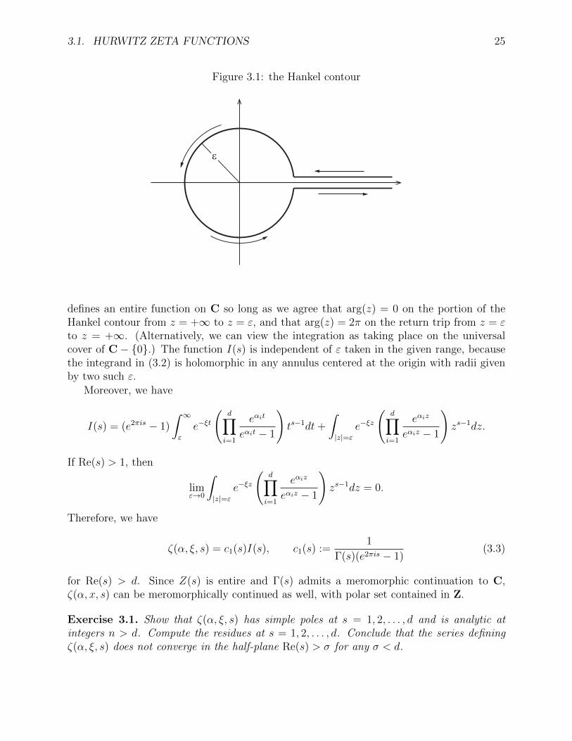
For ε > 0, we let C(∞, ε) be the Hankel contour — the path that traces the real axis from∞ to ε, circles the origin counterclockwise along |z| = ε, and then retraces the real axis fromε to ∞. (See Figure 3.1.)
Suppose ε < 12(2π/minαi). We choose the branch of log(z) such that 0 ≤ arg(z) < 2π.
Then the function
I(s) = I(α, ξ, s) :=
∫C(∞,ε)
e−ξz
(d∏i=1
eαiz
eαiz − 1
)zs−1dz (3.2)
3.1. HURWITZ ZETA FUNCTIONS 25
Figure 3.1: the Hankel contour
ε
defines an entire function on C so long as we agree that arg(z) = 0 on the portion of theHankel contour from z = +∞ to z = ε, and that arg(z) = 2π on the return trip from z = εto z = +∞. (Alternatively, we can view the integration as taking place on the universalcover of C− 0.) The function I(s) is independent of ε taken in the given range, becausethe integrand in (3.2) is holomorphic in any annulus centered at the origin with radii givenby two such ε.
Moreover, we have
I(s) = (e2πis − 1)
∫ ∞ε
e−ξt
(d∏i=1
eαit
eαit − 1
)ts−1dt+
∫|z|=ε
e−ξz
(d∏i=1
eαiz
eαiz − 1
)zs−1dz.
If Re(s) > 1, then
limε→0
∫|z|=ε
e−ξz
(d∏i=1
eαiz
eαiz − 1
)zs−1dz = 0.
Therefore, we have
ζ(α, ξ, s) = c1(s)I(s), c1(s) :=1
Γ(s)(e2πis − 1)(3.3)
for Re(s) > d. Since Z(s) is entire and Γ(s) admits a meromorphic continuation to C,ζ(α, x, s) can be meromorphically continued as well, with polar set contained in Z.
Exercise 3.1. Show that ζ(α, ξ, s) has simple poles at s = 1, 2, . . . , d and is analytic atintegers n > d. Compute the residues at s = 1, 2, . . . , d. Conclude that the series definingζ(α, ξ, s) does not converge in the half-plane Re(s) > σ for any σ < d.
26 CHAPTER 3. SHINTANI’S METHOD
3.2 The Hurwitz zeta functions at nonpositive integers
In this section, we derive formulas for ζ(ξ, α, 1− n), n ≥ 1, when ξ has the form ξ = 〈α, x〉for some x ∈ Rn
≥0, x 6= 0.It is a standard fact that
lims→−m
(s+m)Γ(s) =(−1)m
m!
for nonnegative integers m. It follows that
lims→−m
1
Γ(s)(e2πis − 1)=
(−1)mm!
2πi.
Adapting (3.3), we have
ζ(α, 〈α, x〉, s) =1
Γ(s)(e2πis − 1)
∫C(∞,ε)
d∏i=1
e(1−xi)αiz
eαiz − 1zs−1dz. (3.4)
By the residue theorem, if n ≥ 1, then
ζ(α, 〈α, x〉, 1− n) =(−1)n−1(n− 1)!
2πi· 2πi res
z=0
(d∏i=1
e(1−xi)αiz
eαiz − 1z−n
)
=(−1)n−1(n− 1)!∏d
i=1 αicoeff(F (z), n+ d− 1), (3.5)
where
F (z) =d∏i=1
αize(1−xi)αiz
eαiz − 1.
The Taylor coefficients of F (z) are essentially values of the Bernoulli polynomials, definedby the expansion
zexz
ez − 1=∞∑n=0
Bn(x)zn
n!.
We have the identity of power series
F (z) =d∏i=1
∞∑n=0
Bn(1− xi)αnin!
zn. (3.6)
Combining (3.5) and (3.6), we obtain a useful formula for ζ(α, 〈α, x〉, 0):
ζ(α, 〈α, x〉, 0) = (−1)d∑
r1+···+rd=drj∈Z≥0
d∏j=1
αrj−1j
rj!Brj(xj). (3.7)
Here we have used the fact that Br(1 − x) = (−1)rBr(x). Since the Bernoulli polynomialshave rational coefficients, we have established the following result:
Proposition 3.2. The values ζ(x, α, 1− n), n ≥ 1, belong to the field Q(xi, αi).
3.3. SHINTANI ZETA FUNCTIONS 27
3.2.1 The multiple Γ-function
Finally, recall the classical Hurwitz zeta function ζH(x, s) discussed in §1.1. The Lerchformula relates the derivative of ζH(x, s) at s = 0 to the Γ-function:
∂
∂sζH(x, s)
∣∣s=0
= log
(Γ(x)√
2π
).
Motivated by this formula, we define the multiple Γ-function Γ(x, α) by
log Γ(α, ξ) =∂
∂sζ(α, ξ, s)
∣∣s=0
.
Note thatΓ(x) =
√2πΓ(x, 1).
The multiple log-Γ-function admits meromorphic continuation in ξ to C. To see this, wedifferentiate (3.2) under the integral sign to obtain
I ′(α, ξ, 0) =
∫C(∞,ε)
e−ξz
(d∏i=1
eαiz
eαiz − 1
)log(z)
dz
z. (3.8)
Combined with (3.3), this yields
log Γ(α, ξ) = c′1(0)I(α, ξ, 0) + c1(0)
∫C(∞,ε)
e−ξz
(d∏i=1
eαiz
eαiz − 1
)log(z)
dz
z. (3.9)
The function I(α, ξ, 0) is meromorphic in ξ, as is the function defined by the integral on theright. The meromorphic continuability of log Γ(α, ξ) follows.
3.3 Shintani zeta functions
Shintani axiomatized and enlarged the class of functions whose meromorphic continuationcan be established using the techniques of the previous subsection plus an ingenious changeof variable. Let a = (aji ) ∈ Mn×d(C) such that Re(aji ) > 0 for all i, j and let x ∈ Rd
≥0 be anonzero column vector. We write ai and aj i-th row and the j-th column of a, respectively.Define the Shintani zeta function
ζ(a, x, s) =∑k∈Zd≥0
N(a(x+ k)
)−s(Re(s) > d/n), (3.10)
where x and k are viewed as column vectors, and the “norm” Nv of a vector v ∈ Rn isdefined to be
Nv = v1 · · · vn.
Remark 3.3. If F is a number field of degree n and x 7→ xi are the embeddings of F intoC, then Nx = NF/Q(x).

28 CHAPTER 3. SHINTANI’S METHOD
The multiple Hurwitz zeta function is simply the special case n = 1 of the Shintani zetafunction.
The convergence of the series (3.10) is governed by that of∑k∈Z>0
(k1 + · · ·+ kd)−nσ.
By the discussion of the previous section, this series converges absolutely when nσ > d, orequivalently, when σ > d/n.
By Euler’s trick, we obtain∫ ∞0
e−ai(x+k)tits−1i dti = Γ(s)(ai(x+ k))−s. (3.11)
We write t for the row vector (t1, . . . , tn) and ts−1dt for (t1 · · · tn)s−1dt1 · · · dtn. Taking theproduct of (3.11) over i = 1, . . . , n, we are led to
Γ(s)n N(a(x+ k)
)−s=
∫(0,∞)n
e−ta(x+k)ts−1dt
=
∫(0,∞)n
e−taxe−takts−1dt.
Summing over k, we have
Γ(s)nζ(a, x, s) =
∫(0,∞)n
e−tax∑k∈Zm≥0
e−takts−1dt.
Noting the geometric series
∑k∈Zd≥0
e−tak =d∏j=1
1
1− e−taj=
d∏j=1
etaj
etaj − 1,
we have
Γ(s)nζ(a, x, s) =
∫(0,∞)n
G(t)ts−1dt,
where
G(t) = e−taxd∏j=1
etaj
etaj − 1=
d∏j=1
etaj(1−xj)
etaj − 1. (3.12)
It is tempting to attempt to adapt Riemann’s Hankel contour method for obtaininga meromorphic continuation of ζ(a, x, s) to the complex plane. Unfortunately, a directapplication of the method fails: the hyperplane (aj)⊥ ⊂ Cn has positive dimension if n > 1,and thus interects any polydisk centred at 0 ∈ Cn. Therefore, G(t) will have a singularityalong C(∞, ε1)×· · ·×C(∞, εn) for all choices of εi > 0. Shintani circumvented these analytic

3.3. SHINTANI ZETA FUNCTIONS 29
difficulties by decomposing the domain Rn>0 of integration and applying a change of variable.
We describe his method. Set
Dk = (t1, . . . , tn) ∈ Rn>0 : tj ≤ tk for all j,
and
zk(a, x, s) = Γ(s)−n∫Dk
G(t)ts−1dt. (3.13)
We have
Rn>0 =
n∐k=1
Dk and ζ(a, x, s) =n∑k=1
zk(a, x, s). (3.14)
Consider the change of variable
t = uy = u(y1, . . . , yn), t ∈ Dk,
where u = tk > 0. Since t ∈ Dk, we have 0 ≤ yj ≤ 1 for all j and yk = 1. Substitutingin (3.14), we have
zk(x, a, s) = Γ(s)−n∫
(0,∞)
uns−1
∫(0,1)n−1
G(uy)ys−1dy
du, (3.15)
where we have written
y = (y1, . . . , yk−1, 1, yk+1, . . . , yn) ∈ Rn, y = (y1, . . . , yk−1, yk+1, . . . , yn) ∈ Rn−1,
andys−1dy :=
∏j 6=k
ys−1j dyj.
Set
cn(s) =1
(e2πins − 1)(e2πis − 1)n−1Γ(s)n(3.16)
and let C(1, ε) be the subcontour of C(∞, ε) that starts and ends at z = 1 instead of atz = +∞.
Proposition 3.4. For sufficiently small ε, we have
zk(a, x, s) = cn(s)
∫C(∞,ε)
uns−1
∫C(1,ε)n−1
G(uy)ys−1dy
du. (3.17)
The iterated line integral on the right is absolutely convergent and defines a meromorphicfunction of s that is independent of ε, provided ε is sufficiently small.
Proof. Set
Ik,ε(s) = Ik,ε(a, x, s) =
∫C(∞,ε)
uns−1
∫C(1,ε)n−1
G(uy)ys−1dy
du. (3.18)
30 CHAPTER 3. SHINTANI’S METHOD
First we verify that, for sufficiently small epsilon, the integrand has no singularities alongC(∞, ε) × C(1, ε)n−1. We must show that, for ε sufficiently small, uyaj is not an integermultiple of 2πi. By the Cauchy-Schwartz inequality, we can find ε1 > 0 such that
|uyaj| ≤ ‖uy‖ · ‖aj‖ < 1 (j = 1, . . . , d),
whenever |u| < ε1. On the other hand,
limy→0
yaj = ajk.
Therefore, we may find ε2 > 0 such that
Re(yaj) >1
2minRe(aji ) : i = 1, . . . , n > 0, j = 1, . . . , d,
whenever |yi| < ε2 for all i 6= k. (This is where we use our assumption that the entries of ahave positive real part.) In particular, yaj is nonzero for these y. Letting ε0 = minε1, ε2,we have 0 < |uyaj| < 1 whenever |u| < ε1 and |yi| < ε1 for all i 6= k. Thus, uyaj is nota multiple of 2πi for these u, y, and the holomorphy of Ik,ε(s) follows. Cauchy’s theoremimplies that Ik,ε(s) is independent of ε for ε < ε0. Therefore, we may denote this functionsimply by Ik(s) = Ik(a, x, s).
Let ε < ε0. By arguments similar to those of the previous section,
Ik(s) =
∫|u|=ε
uns−1
∫|yi|=εi 6=k
G(uy)ys−1dy
du+
(e2πins − 1)(e2πis − 1)n−1
∫(ε,∞)
uns−1
∫(ε,1)n−1
G(uy)ys−1dy
du.
If s > d/n, then a trivial estimate shows that
limε→0
∫|u|=ε
uns−1
∫|yi|=εi 6=k
G(uy)ys−1dy
du = 0.
Therefore,
Ik(s) = (e2πins − 1)(e2πis − 1)n−1
∫(0,∞)
uns−1
∫(0,1)n−1
G(uy)ys−1dy
du
= (e2πins − 1)(e2πis − 1)n−1Γ(s)nzk(a, x, s)
= cn(s)−1zk(a, x, s).
Exercise 3.5. Find the poles of ζ(a, x, s), their orders, and their residues.
Exercise 3.6. Show how to define and meromorphically continue the more general Shintanizeta function
ζ(a, x, (s1, . . . , sn)) =∑k∈Zd≥0
n∏i=1
(ai(x+ k))−si .

3.4. SPECIAL VALUES OF SHINTANI ZETA FUNCTIONS 31
3.4 Special values of Shintani zeta functions
In this section, we give Shintani’s formulas for the values of ζ(a, x, s) when s is a nonpositiveinteger. We first consider the special case s = 0, particularly important from the point ofview of Stark’s conjecture. The residue of Γ(s) at s = 0 is 1, and hence
lims→0
cn(s) =1
n(2πi)n, cn(s) :=
1
(e2πins − 1)(e2πis − 1)n−1Γ(s)n.
Therefore, (3.17) becomes
zk(a, x, 0) =1
n(2πi)nIk(0) =
1
n(2πi)n
∫C(∞,ε)
u−1
∫C(1,ε)n−1
G(uy)y−1dy
du.
Observe that G(uy) is holomorphic in the variables yi, i 6= k. Therefore, by the residuetheorem, ∫
C(1,ε)n−1
G(uy)∏i 6=k
dyiyi
= G(0, . . . , 0, u, 0, . . . , 0)
= (2πi)n−1
d∏j=1
e(1−xj)ajku
eajku − 1
. (3.19)
Thus, by (3.4) and (3.7),
zk(a, x, 0) =1
n(2πi)
∫C(∞,ε)
d∏j=1
e(1−xj)ajku
eajku − 1
du
u
=1
nζ(ak, 〈ak, x〉, 0) (3.20)
=(−1)d
n
∑`∈Zd≥0
`1+···+`d=d
d∏j=1
B`j(xj)(ajk)
`j−1
`j!. (3.21)
Proposition 3.7. We have:
ζ(a, x, 0) =(−1)d
n
n∑k=1
∑`∈Zd≥0
`1+···+`d=d
d∏j=1
B`j(xj)(ajk)
`j−1
`j!. (3.22)
Corollary 3.8. The value ζ(a, x, 0) belongs to the field generated by the components of xand the entries of a.
We record the n = d = 2 case of this formula for later use. Writing
w =
(w1
w2
), a =
(p qr s
),
we have
ζ(a, w, 0) =1
4
(p
q+r
s
)B2(w1) + 4B1(w1)B2(w2) +
(q
p+s
r
)B2(w2)
. (3.23)

32 CHAPTER 3. SHINTANI’S METHOD
3.4.1 Generalized Bernoulli polynomials
To evaluate ζ(a, x, 1 − n) for n ≥ 1, we define generalized Bernoulli polynomials Bk,m(a, x)by
Bk,m(a,1− x)
(m!)n= coeff
(G(uy), (uny1 · · · yk−1yk+1 · · · yn)m−1
), (3.24)
where 1 is the vector (1, . . . , 1).
Theorem 3.9 ([26, Proposition 1]). Let m ≥ 1 be an integer. Then
ζ(a, x, 1−m) =(−1)n(m−1)
n
n∑k=1
Bk,m(a,1− x)
mn.
Proof. Applying the residue theorem a total of n times, we have
Ik,ε(1−m) =
∫C(∞,ε)
un(1−m)−1
∫C(1,ε)n−1
G(uy)y−mdy
du
= 2πi coeff((2πi)n−1 coeff(G(uy), ym−1), un(m−1))
= (2πi)nBk,m(a,1− x)
(m!)n.
Since
lims→1−m
(e2πins − 1)(e2πis − 1)n−1Γ(s)n = n
((−1)m−12πi
(m− 1)!
)nwe conclude using Proposition 3.4 that
zk(a, x, 1−m) =(−1)n(m−1)
n
Bk,m(1− x)
mn.
The desired result follows from (3.14).
Exercise 3.10. Express the generalized Bernoulli polynomial Bk,m(a, x) in terms of thestandard Bernoulli polynomials Bk.
Corollary 3.11. The value ζ(a, x, 1 −m) belongs to the field generated by the componentsof x and the entries of a.
3.4.2 An algebraic version of Shintani’s formula
Recall that the singularity of
G(t) =d∏j=1
e(1−xi)taj
etaj − 1.

3.4. SPECIAL VALUES OF SHINTANI ZETA FUNCTIONS 33
at t = 0 is not isolated, implying that G(t) does not have a convergent Laurent expansionin any punctured neighbourhood of t = 0. Nevertheless, for j = 1, . . . , d, we may define
Gj(t) =
taj
etaj − 1if taj 6= 0,
1, otherwise.
The functions Gj(t) are holomorphic at t = 0 and thus have convergent Taylor expansions
Gj(t) ∈ C[[t]] := C[[t1, . . . , tn]].
Since∏d
j=1 taj ∈ C[t] ⊂ C[[t]], we may identify G(t) as a quotient
G(t) =d∏j=1
Gj(t)e(1−xi)taj
taj∈ C((t)),
where C((t)) denotes the field of fractions of C[[t]]. Caution is required when workingwith the field C((t)) because, unless n = 1, its elements are not simply formal sums ofmonomials tm, m ∈ Zn. In particular, it does not make sense to talk about the coefficientof tm appearing in a general element of C((t)) when n > 1. However, we make the followingtrivial observation:
Lemma 3.12. Let h(t) ∈ C[t] be a homogeneous polynomial of degree r such that
coeff(h(t), trk) 6= 0,
let g(t) ∈ C[[t]], and let f(t) = g(t)/h(t). Then
f(tk(t1, . . . , tk−1, 1, tk+1, . . . tn)) ∈ t−rk C[[t]].
If f(t) is as in the lemma, then the expression
coeff(f(tk(t1, . . . , tk−1, 1, tk+1, . . . tn)), tm) (3.25)
is well defined for all t ∈ Zn. Now, G(t) has the property of Lemma 3.12 with h(t) =∏d
j=1 taj
(recall that each aji has positive real part and in particular is non-zero). Therefore it makessense to discuss the coefficients (3.25) for the algebraic object G(t) ∈ C((t)); these coefficientsencode the values of ζ(a, x, s) at nonpositive integers, as described in the following corollary.
Corollary 3.13. Let m be a nonnegative integer. Then
ζ(a, x,−m) = ∆(m)G :=((−1)mm!)n
n×
n∑k=1
coeff (G(tk(t1, . . . , tk−1, 1, tk, . . . , tn)), (t1 · · · tk−1tnktk+1 · · · tn)m) .

34 CHAPTER 3. SHINTANI’S METHOD
3.5 Derivatives of Shintani zeta functions at s = 0
Recall that by Proposition 3.4, we have
zk(a, x, s) = cn(s)Ik(a, x, s).
(These functions were defined in (3.13), (3.16), and (3.18).) Therefore,
z′k(a, x, 0) = c′n(0)Ik(a, x, 0) + cn(0)I ′k(a, x, 0)
= c′n(0)(2πi)n−1I(ak, 〈ak, x〉, 0) + cn(0)I ′k(a, x, 0), (3.26)
Differentiating under the integral sign,
I ′k(a, x, 0) = n
∫C(∞,ε)
log(u)
∫C(1,ε)n−1
G(uy)dy
y
du
u(3.27)
+ cn(0)−1∑i 6=k
δk,i(a, x) (3.28)
where
δk,i(a, x) = cn(0)
∫C(∞,ε)
∫C(1,ε)n−1
G(uy) log(yi)dy
y
du
u(i 6= k).
By (3.19), the term from (3.27) may be written
n(2πi)n−1
∫C(∞,ε)
log(u)d∏j=1
e(1−xj)ajku
eajku − 1
du
u
=n(2πi)n−1
c1(0)(log Γ(ak, 〈ak, x〉)− c′1(0)I(ak, 〈ak, x〉, 0)) , (3.29)
Here (3.29) follows from (3.9).Combining (3.26)–(3.29) and applying the identities
cn(0)n(2πi)n−1 = c1(0), c′n(0)(2πi)n−1 = c′1(0),
we see thatz′k(a, x, 0) = log Γ(ak, 〈ak, x〉) +
∑i 6=k
δk,i(a, x). (3.30)
The terms δk,i(a, x) can be evaluated in “elementary” terms:
δk,i(a, x) =(−1)d
n
d∑j=1
∑`∈Zd≥0
`1+···+`d=d`j=0
(log(ajk)− log(ajk + aji ))∏r 6=j
B`r(xr)
`r!
(arkajk− ariaji
)`r−1
. (3.31)
Note that for all i, j, k,
∏r 6=k
(arkajk− ariaji
)`r−1
= −∏r 6=k
(ariaji− arkajk
)`r−1
.

3.5. DERIVATIVES OF SHINTANI ZETA FUNCTIONS AT S = 0 35
Therefore,n∑k=1
∑i 6=k
δk,i(a, x) =n∑k=1
δk(a, x),
where
δk(a, x) =(−1)d
n
d∑j=1
∑`∈Zd≥0
`1+···+`d=d`j=0
log(ajk)∏r 6=j
B`r(xr)
`r!
(arkajk− ariaji
)`r−1
, (3.32)
and we havez′k(a, x, 0) = Γ(ak, 〈ak, x〉, 0) + δk(a, x).
Combining with (3.14), we obtain
ζ ′(a, x, 0) =n∑k=1
(Γ(ak, 〈ak, x〉, 0) + δk(a, x)
). (3.33)
This formula will be used in the construction of Stark units in the ATR case.
3.5.1 The multiple sine function
Suppose now that, in addition to previously imposed hypotheses, we have 0 ≤ Re(xj) ≤ 1and 1− Re(x) 6= 0, where 1 = (1, . . . , 1) ∈ Rd. Define
ζ+(a, x, s) = −ζ(a, x, s) + (−1)dζ(a,1− x, s).
By 3.7 and the identityB`(t) = (−1)`B`(1− t), (3.34)
we haveζ+(a, x, 0) = 0.
Thus, it is very natural to consider the derivative of ζ+(a, x, s) at s = 0. We define theShintani sine function by
S(x, a) = exp
(d
dsζ+(x,A, s)
∣∣∣∣∣s=0
).
Applying (3.34) again, we see that
δk(a, x) + (−1)dδk(a,1− x) = 0.
Therefore,
S(a, x) = (ζ+)′(a, x, 0) =n∑k=1
(ζ+)′(ak, 〈ak, x〉, 0) =n∑k=0
S(ak, 〈x, ak〉).
We will apply this formula later to our study of Stark’s conjecture in the TR∞ case.
36 CHAPTER 3. SHINTANI’S METHOD
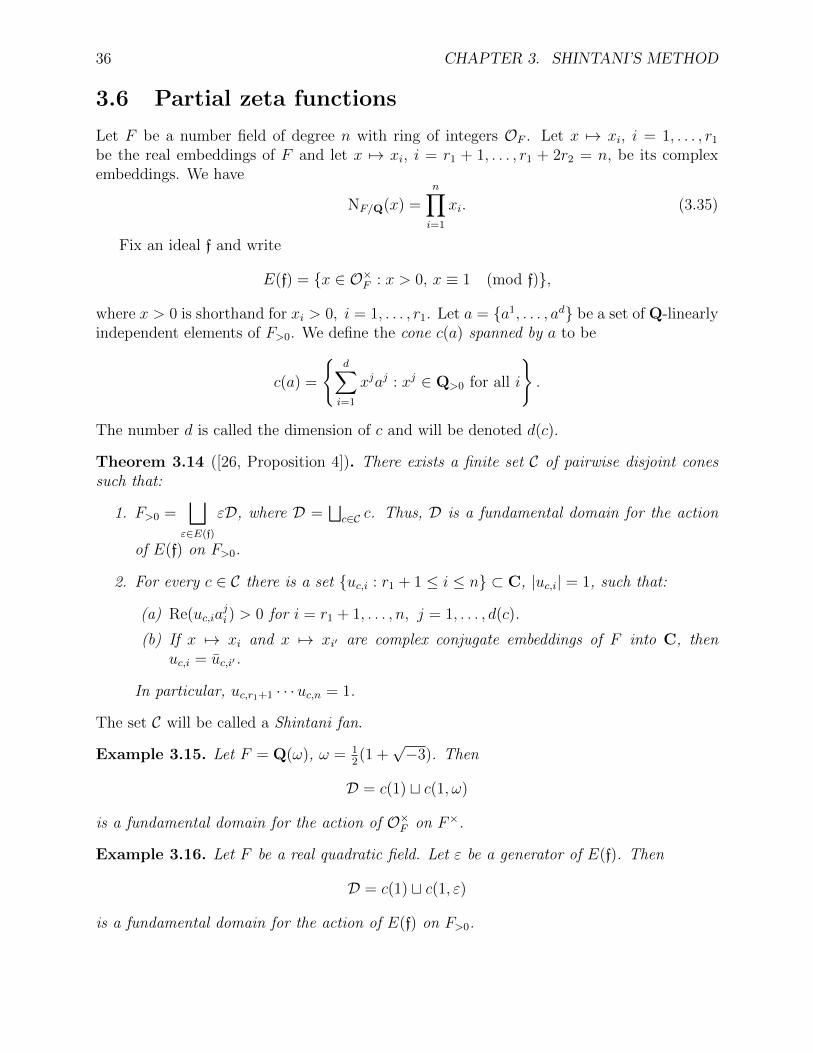
3.6 Partial zeta functions
Let F be a number field of degree n with ring of integers OF . Let x 7→ xi, i = 1, . . . , r1
be the real embeddings of F and let x 7→ xi, i = r1 + 1, . . . , r1 + 2r2 = n, be its complexembeddings. We have
NF/Q(x) =n∏i=1
xi. (3.35)
Fix an ideal f and write
E(f) = x ∈ O×F : x > 0, x ≡ 1 (mod f),
where x > 0 is shorthand for xi > 0, i = 1, . . . , r1. Let a = a1, . . . , ad be a set of Q-linearlyindependent elements of F>0. We define the cone c(a) spanned by a to be
c(a) =
d∑i=1
xjaj : xj ∈ Q>0 for all i
.
The number d is called the dimension of c and will be denoted d(c).
Theorem 3.14 ([26, Proposition 4]). There exists a finite set C of pairwise disjoint conessuch that:
1. F>0 =⊔
ε∈E(f)
εD, where D =⊔c∈C c. Thus, D is a fundamental domain for the action
of E(f) on F>0.
2. For every c ∈ C there is a set uc,i : r1 + 1 ≤ i ≤ n ⊂ C, |uc,i| = 1, such that:
(a) Re(uc,iaji ) > 0 for i = r1 + 1, . . . , n, j = 1, . . . , d(c).
(b) If x 7→ xi and x 7→ xi′ are complex conjugate embeddings of F into C, thenuc,i = uc,i′.
In particular, uc,r1+1 · · ·uc,n = 1.
The set C will be called a Shintani fan.
Example 3.15. Let F = Q(ω), ω = 12(1 +
√−3). Then
D = c(1) t c(1, ω)
is a fundamental domain for the action of O×F on F×.
Example 3.16. Let F be a real quadratic field. Let ε be a generator of E(f). Then
D = c(1) t c(1, ε)
is a fundamental domain for the action of E(f) on F>0.
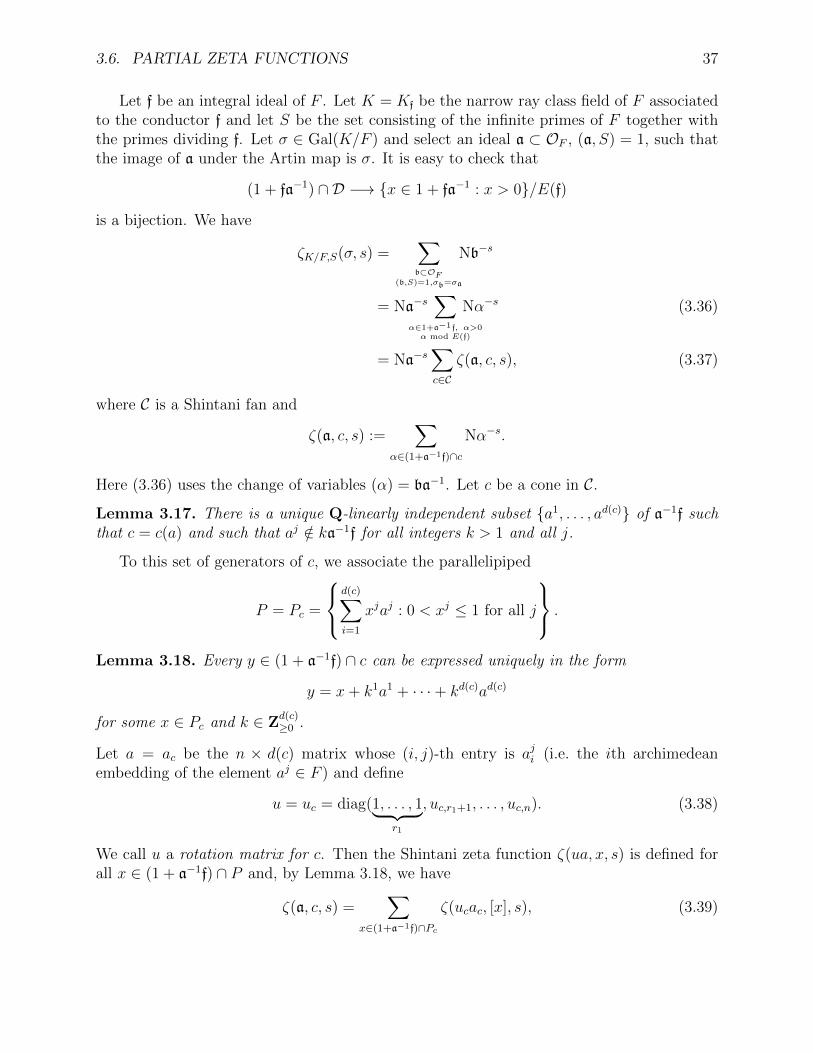
3.6. PARTIAL ZETA FUNCTIONS 37
Let f be an integral ideal of F . Let K = Kf be the narrow ray class field of F associatedto the conductor f and let S be the set consisting of the infinite primes of F together withthe primes dividing f. Let σ ∈ Gal(K/F ) and select an ideal a ⊂ OF , (a, S) = 1, such thatthe image of a under the Artin map is σ. It is easy to check that
(1 + fa−1) ∩ D −→ x ∈ 1 + fa−1 : x > 0/E(f)
is a bijection. We have
ζK/F,S(σ, s) =∑b⊂OF
(b,S)=1,σb=σa
Nb−s
= Na−s∑
α∈1+a−1f, α>0α mod E(f)
Nα−s (3.36)
= Na−s∑c∈C
ζ(a, c, s), (3.37)
where C is a Shintani fan and
ζ(a, c, s) :=∑
α∈(1+a−1f)∩c
Nα−s.
Here (3.36) uses the change of variables (α) = ba−1. Let c be a cone in C.
Lemma 3.17. There is a unique Q-linearly independent subset a1, . . . , ad(c) of a−1f suchthat c = c(a) and such that aj /∈ ka−1f for all integers k > 1 and all j.
To this set of generators of c, we associate the parallelipiped
P = Pc =
d(c)∑i=1
xjaj : 0 < xj ≤ 1 for all j
.
Lemma 3.18. Every y ∈ (1 + a−1f) ∩ c can be expressed uniquely in the form
y = x+ k1a1 + · · ·+ kd(c)ad(c)
for some x ∈ Pc and k ∈ Zd(c)≥0 .
Let a = ac be the n × d(c) matrix whose (i, j)-th entry is aji (i.e. the ith archimedeanembedding of the element aj ∈ F ) and define
u = uc = diag(1, . . . , 1︸ ︷︷ ︸r1
, uc,r1+1, . . . , uc,n). (3.38)
We call u a rotation matrix for c. Then the Shintani zeta function ζ(ua, x, s) is defined forall x ∈ (1 + a−1f) ∩ P and, by Lemma 3.18, we have
ζ(a, c, s) =∑
x∈(1+a−1f)∩Pc
ζ(ucac, [x], s), (3.39)

38 CHAPTER 3. SHINTANI’S METHOD
where [x] ∈ Qd≥0 is the coefficient vector of x with respect to the columns of ac, i.e. such that
x =∑d(c)
j=1[x]jaj. In (3.39), we have used the fact that uc,r1+1 · · ·un = 1 along with (3.35). It
follows that
ζK/F,S(σ, s) = Na−s∑c∈C
∑x∈(1+a−1f)∩Pc
ζ(ucac, [x], s) (3.40)
= Na−s∑c∈C
∑x∈(1+a−1f)∩Pc
n∑k=1
zk(ucac, [x], s). (3.41)
Corollary 3.19. The partial zeta function ζK/F,S(σ, s) admits a meromorphic continuationto the whole complex plane and takes on rational values at nonpositive integral arguments.
Exercise 3.20. Suppose F has at least one complex place and |S| ≥ 2. Show that ζS(σ, n) = 0for n < 0. Hint: Think about the gamma factors in the functional equation.
3.7 Shintani decompositions of partial zeta functions
We can use the decomposition of Shintani zeta functions in (3.14) to decompose ζS(σ, s).Define
zk(a, C, uc, s) =∑c∈C
∑x∈(1+a−1f)∩Pc
zk(ucac, [x], s), (3.42)
where [x] ∈ Qd≥0 is the coordinate vector of x with respect to the columns of ac. As we shall
see, the existence of this decomposition is the key to all the conjectural, archimedean Starkunit constructions based on Shintani-type methods. To obtain well-defined candidates forStark units, we must analyze the dependence of zk(a, C, uc, 0) and z′k(a, C, uc, 0) on thechoices of a, C and uc.
3.7.1 Dependence on rotation matrices
Proposition 3.21. Suppose u and v are diagonal matrices such that all the entries of auand av have positive real part.
1. We have ζ(ua, x, 0) = ζ(va, x, 0). More precisely,
ζ(ua, x, 0) =(−1)d
n
n∑k=1
∑`∈Zd≥0
`1+···`d=d
d∏j=1
B`j(xj)
`j!(ajk)
`j−1.
2. Suppose that a = ac and u = uc where c = c(a1, . . . , ad) is a cone in F>0 and thatx ∈ Q2
≥0, x 6= 0. Then
ζ(ua, x, 0) = TrF/Q
(−1)d
n
∑`∈Zd≥0
`1+···`d=d
d∏j=1
B`j(xj)
`j!(aj)`i−1
∈ Q.

3.7. SHINTANI DECOMPOSITIONS OF PARTIAL ZETA FUNCTIONS 39
3. Let vc be another rotation matrix for c and let N be a positive integer such thatζ(x, ua, 0) ∈ 1
NZ. Then
z′k(ua, x, 0)− ζ(a, x, 0) log(uk) ≡ z′k(va, x, 0)− ζ(0, a, x) log(vk) (mod 2πiN
Z)
for k = 1, . . . , n.
Remark 3.22. The formula for ζ(ua, x, 0) in 1. is the same as that appearing in (3.22).Thus, rotation matrices have no effect on the values of Shintani zeta functions at s = 0.
Proof. The deduction of 1. and 2. from previous results is left as an exercise for the reader.For a proof of 3., see [20, Proposition 2] case v = 1.
Setting
ϕk(a, u, x) = z′k(ua, x, 0)− ζ(ua, x, 0) log(uk),
Φk(a, C, uc) =∑c∈C
∑xc∈(1+a−1f)∩Pc
ϕk(ac, uc, xc)
we have shown that the cosets ϕk(a, u, x)+ 2πiN
Z and Φk(a, C, uc)+ 2πiN
Z are independent ofthe rotation matrix u. Since rotations corresponding to conjugate embeddings are conjugate,we obtain from (3.41):
n∑k=1
Φk(a, C, uc) ≡ ζ ′S(σa, 0) (mod 2πiN
Z) (3.43)
when ζK/F,S(σa, 0) = 0. This decomposition of ζ ′S(σa, 0) is the key to the refinement of Stark’sconjecture in the ATR case.
3.7.2 Dependence on the cover
We say that (C ′, uc′) is a refinement or simplicial subdivision of (C, uc) if
1. C ′ can be partitioned into subsets C ′c, c ∈ C, such that each c is the disjoint union ofthe simplicial cones c′ ∈ C ′c;
2. For each c′ ∈ C ′c, we have uc′ = uc.
Proposition 3.23.
1. The quantity Φk(a, C, uc) is invariant under refinement of C.
2. Let (C, uc) and (D, ud) be as in Theorem 3.14. Then there an unit η ∈ E(f) suchthat
Φk(a,D, ud) ≡ Φk(a, C, uc)−1
Nlog ηk (mod 2πi
NZ).

40 CHAPTER 3. SHINTANI’S METHOD
Remark 3.24. The proof of statement 1. is the technical heart of the paper [20].
Proof. Let c be a simplicial, let a = ac be its matrix of generators, and let u = uc be anassociated rotation matrix. To show that
ϕk(a, u, x) = z′k(ua, x, 0) + ζ(ua, x, 0) log(uk)
= log Γ(uak, 〈uak, x〉) + δk(ua, x) + ζ(ua, x, 0) log(uk)
is invariant under simplicial subdivision, we consider its three constituents separately. Toshow that log Γ(uak, 〈uak, x〉) and ζ(ua, x, 0) are invariant under simplicial subdivision of cis a routine exercise. Showing that δk(ua, x) is similarly invariant is hard, technical work.We refer the reader to [20, Lemma 1] for details.
We prove 2. As⋃C and
⋃D may be different fundamental domains for the action of
E(f) on F>0, there need be no common refinement. However, by 1., we may assume thefollowing property is satisfied: For each c ∈ C there is a unique unit ηc ∈ E(f), such thatcηc ∈ D. Since
⋃C and
⋃D are both fundamental domains for the action of E(f) on F>0,
we must have D = cηc : c ∈ C.Set
δc = diag(η(1)c , . . . , η(n)
c ), vc = ucδ−1c .
Noting that acηc = δcac, we see that the entries of the matrices vcacηc = ucac have positivereal parts. We have:
ϕk(acηc , vc, x) = ϕk(δcac, ucδ−1c , x)
≡ ϕk(ac, uc, x)− ζ(ucac, x, 0) log η(k)c (mod 2πi
NZ)
by statement 3. of Proposition 3.21. Since ηc ≡ 1 (mod f), we have
(1 + a−1f) ∩ Pcηc = ((1 + a−1f) ∩ Pc)ηc.
Therefore,
Φk(a,D, vc) ≡ Φk(a, C, uc)−∑c∈C
∑(1+a−1f)∩Pcηc
ζ(ucac, x, 0) log(η(k)c ) (mod 2πi
NZ).
For each c and x, lett(c, x) = Nζ(ucac, x, 0) ∈ Z.
Then ∑c∈C
∑(1+a−1f)∩Pcηc
ζ(ucac, x, 0) log(η(k)c ) =
1
Nlog η(k),
whereη :=
∏c∈E
∏(1+a−1f)∩Pcηc
ηt(c,x)c ,
and we have
Φk(a,D, vc) ≡ Φk(a, C, uc)−1
Nlog η(k) (mod 2πi
NZ).
This proves 2., completing the proof.
3.8. KRONECKER’S LIMIT FORMULA AND SHINTANI ZETA FUNCTIONS 41
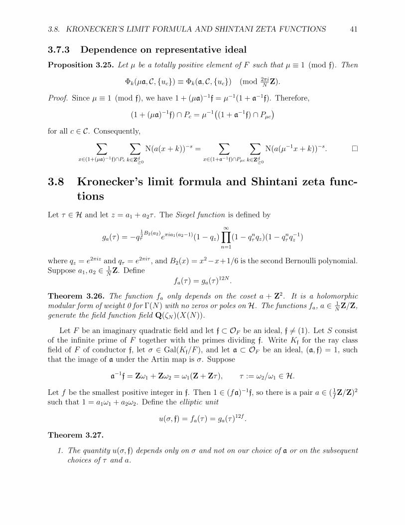
3.7.3 Dependence on representative ideal
Proposition 3.25. Let µ be a totally positive element of F such that µ ≡ 1 (mod f). Then
Φk(µa, C, uc) ≡ Φk(a, C, uc) (mod 2πiN
Z).
Proof. Since µ ≡ 1 (mod f), we have 1 + (µa)−1f = µ−1(1 + a−1f). Therefore,
(1 + (µa)−1f) ∩ Pc = µ−1((1 + a−1f) ∩ Pµc
)for all c ∈ C. Consequently,∑
x∈(1+(µa)−1f)∩Pc
∑k∈Zd≥0
N(a(x+ k))−s =∑
x∈(1+a−1f)∩Pµc
∑k∈Zd≥0
N(a(µ−1x+ k))−s.
3.8 Kronecker’s limit formula and Shintani zeta func-
tions
Let τ ∈ H and let z = a1 + a2τ . The Siegel function is defined by
ga(τ) = −q12B2(a2)
τ eπia1(a2−1)(1− qz)∞∏n=1
(1− qnτ qz)(1− qnτ q−1z )
where qz = e2πiz and qτ = e2πiτ , and B2(x) = x2−x+1/6 is the second Bernoulli polynomial.Suppose a1, a2 ∈ 1
NZ. Define
fa(τ) = ga(τ)12N .
Theorem 3.26. The function fa only depends on the coset a + Z2. It is a holomorphicmodular form of weight 0 for Γ(N) with no zeros or poles on H. The functions fa, a ∈ 1
NZ/Z,
generate the field function field Q(ζN)(X(N)).
Let F be an imaginary quadratic field and let f ⊂ OF be an ideal, f 6= (1). Let S consistof the infinite prime of F together with the primes dividing f. Write Kf for the ray classfield of F of conductor f, let σ ∈ Gal(Kf/F ), and let a ⊂ OF be an ideal, (a, f) = 1, suchthat the image of a under the Artin map is σ. Suppose
a−1f = Zω1 + Zω2 = ω1(Z + Zτ), τ := ω2/ω1 ∈ H.
Let f be the smallest positive integer in f. Then 1 ∈ (fa)−1f, so there is a pair a ∈ ( 1fZ/Z)2
such that 1 = a1ω1 + a2ω2. Define the elliptic unit
u(σ, f) = fa(τ) = ga(τ)12f .
Theorem 3.27.
1. The quantity u(σ, f) depends only on σ and not on our choice of a or on the subsequentchoices of τ and a.
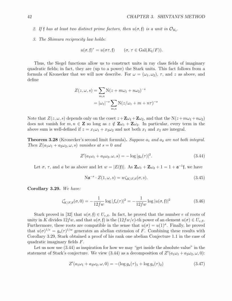
42 CHAPTER 3. SHINTANI’S METHOD
2. If f has at least two distinct prime factors, then u(σ, f) is a unit in OKf.
3. The Shimura reciprocity law holds:
u(σ, f)τ = u(στ, f) (σ, τ ∈ Gal(Kf/F )).
Thus, the Siegel functions allow us to construct units in ray class fields of imaginaryquadratic fields; in fact, they are (up to a power) the Stark units. This fact follows from aformula of Kronecker that we will now describe. For ω = (ω1, ω2), τ , and z as above, anddefine
Z(z, ω, s) =∑m,n
N(z +mω1 + nω2)−s
= |ω1|−s∑m,n
N(z/ω1 +m+ nτ)−s
Note that Z(z, ω, s) depends only on the coset z+Zω1 +Zω2, and that the N(z+mω1 +nω2)does not vanish for m,n ∈ Z so long as z /∈ Zω1 + Zω2. In particular, every term in theabove sum is well-defined if z = x1ω1 + x2ω2 and not both x1 and x2 are integral.
Theorem 3.28 (Kronecker’s second limit formula). Suppose a1 and a2 are not both integral.Then Z(a1ω1 + a2ω2, ω, s) vanishes at s = 0 and
Z ′(a1ω1 + a2ω2, ω, s) = − log |ga(τ)|2. (3.44)
Let σ, τ , and a be as above and let w = |E(f)|. As Zω1 + Zω2 + 1 = 1 + a−1f, we have
Na−s · Z(1, ω, s) = wζK/F,S(σ, s). (3.45)
Corollary 3.29. We have:
ζ ′K/F,S(σ, 0) = − 1
12fwlog |fa(τ)|2 = − 1
12fwlog |u(σ, f)|2 (3.46)
Stark proved in [32] that u(σ, f) ∈ Uv,S. In fact, he proved that the number e of roots ofunity in K divides 12fw, and that u(σ, f) is the (12fw/e)-th power of an element u(σ) ∈ Uv,S.Furthermore, these roots are compatible in the sense that u(σ) = u(1)σ. Finally, he provedthat u(σ)1/e = ga(τ)1/w generates an abelian extension of F . Combining these results withCorollary 3.29, Stark obtained a proof of his rank one abelian Conjecture 1.1 in the case ofquadratic imaginary fields F .
Let us now use (3.44) as inspiration for how we may “get inside the absolute value” in thestatement of Stark’s conjecture. We view (3.44) as a decomposition of Z ′(a1ω1 + a2ω2, ω, 0):
Z ′(a1ω1 + a2ω2, ω, 0) = −(log ga(τ)1 + log ga(τ)2) (3.47)
3.8. KRONECKER’S LIMIT FORMULA AND SHINTANI ZETA FUNCTIONS 43
into two components corresponding to the embeddings x 7→ xi, i = 1, 2, of F into C. We haveseen such decompositions already, namely (3.43) in the context of Shintani zeta functions.These phenomena are related: Note that we may write
Z(z, ω, s) =∑
m∈Z2≥0
N(z +m1ω1 +m2ω2)−s
+∑
m∈Z2≥0
N(z + (−1−m1)ω1 +m2ω2)−s
+∑
m∈Z2≥0
N(z +m1ω1 + (−1−m2)ω2)−s
+∑
m∈Z2≥0
N(z + (−1−m1)ω1 + (−1−m2)ω2)−s. (3.48)
Assume that E(f) = 1. Then the above decomposition of Z(z, ω, s) corresponds to anexpression of Z(s, ω, s) as a combination of Shintani zeta functions. By (3.48), z /∈ Zω1+Zω2
implies that
z + Zω1 + Zω2 = (z + Zω1 + Zω2) ∩⋃
σ∈±2cσ,
where
c++ = c(ω1, ω2), c−+ = c(−ω1, ω2, ), c−− = c(−ω1,−ω2), c+− = c(ω1,−ω2).
Let uσ be a rotation matrix for cσ and write aσ for acσ , σ ∈ ±2. Then
Z(z, ω, s) =∑
σ∈±2
ζ
(u++a++,
(x1
x2
), s
)+ ζ
(u−+a−+,
(1− x1
x2
), s
)+
ζ
(u−−a−−,
(1− x1
1− x2
), s
)+ ζ
(u+−a+−,
(x1
1− x2
), s
)holds whenever z /∈ Zω1 +Zω2. This holds in particular when z = 1 in which case, by (3.45),we have an expression for ζS(σ, s) as a sum of four Shintani zeta functions. By the followingexercise, this is the decomposition of ζS(σa, s) subordinate to the Shintani fan
C := cσ : σ ∈ ±2.
Exercise 3.30.
1. We may assume without loss of generality that 0 ≤ xi ≤ 1, for i = 1, 2, with strictinequalities for at least one i. Why?
2. Show that
(1 + Zω1 + Zω2) ∩ Pc++ =
(x1
x2
),
and similarly for the other cones in C.

44 CHAPTER 3. SHINTANI’S METHOD
Thus, by (3.43), we have
Φ1(a, C, uc) + Φ2(a, C, uc) ≡ ζ ′S(σa, 0) (mod 2πiN
Z).
Note that Φ1(a, C, uc) and Φ2(a, C, uc) are complex conjugate and that, by statement2. of Proposition 3.23, the cosets
Φk(a, C, uc) +2πi
NwZ (k = 1, 2)
are independent of C. Let us denote these cosets by Φk(a).
Theorem 3.31 ([28]). Let f be the smallest positive integer in f. Then we may take N = fand we have
Φk(a) ≡ − log ga(τ)(k)
(mod
2πi
NwZ
)Since the multiple Γ-functions constitute the main terms of derivatives at s = 0 of
Shintani zeta functions, it is becomes less surprising that Shintani’s method can be used toprove the Kronecker limit formula. The standard construction of the Siegel function uses thetheory of elliptic functions. The prototypical elliptic function, the Weierstrass ℘-function, isintimately related to the double gamma function.
Exercise 3.32. Show that
d3
dz3Γ(z, (ω1, ω2)) = −2
∑m,n
(z +mω1 + nω2)−3 =d
dz℘(z, (ω1, ω2)).
Can you compute the constant
ν :=d2
dz2Γ(z, (ω1, ω2))− ℘(z, (ω1, ω2))?
3.9 Complex cubic fields–the work of Ren and Sczech
Let F be an ATR cubic field with distinct embeddings
x 7→ x1 ∈ R, x 7→ x2 ∈ C, x 7→ x3 ∈ C.
Note that x2 and x3 are complex conjugates for all x ∈ F . Let f, σ, and a all be as in §3.6and let ε be the generator of E(f) such that ε1 > 1. Let (C, uc) be as Theorem 3.14. Define
ϑ(a, C) = ϑ2(a, C) = Φ2(a, C)− Φ1(a, C) log ε2
log ε1
.
Proposition 3.33.
1. The coset ϑ(a, C) + 2πiN
Z does not depend on our choices of a and C.

3.9. COMPLEX CUBIC FIELDS–THE WORK OF REN AND SCZECH 45
2. We have
ϑ(a, C) + ϑ(a, C) = Φ1(a, C) + Φ2(a, C) + Φ3(a, C) = ζ ′S(σ, 0).
Proof. We first consider the dependence on C. Let C ′ be another Shintani fan for F . ByProposition 3.23, there is a unit η ∈ E(f) such that
Φk(a, C ′)− Φk(a, C) ≡1
Nlog η1 (mod 2πi
NZ) (k = 1, 2, 3). (∗k)
Multiplying ∗1 by log(η2)/ log(η1) and subtracting the result from ∗2, we obtain
Φ2(a, C ′)− log η2
log η1
Φ1(a, C ′) ≡ Φ2(a, C)− log η2
log η1
Φ1(a, C) (mod 2πiN
Z).
Since ε generates E(f), η = εm for some m ∈ Z and we have
log(η2)
log(η1)=
log(ε2)
log(ε1).
(This is where we use the fact that we are working with a cubic field.) Therefore, 1. holds.We now prove 2. Since Φ1(a, C) is real and Φ2(a, C) = Φ3(a, C),
ϑ(a, C) + ϑ(a, C) = −Φ1(a, C) log ε(2) + log ε(3)
log ε(1)+ Φ2(a, C) + Φ3(a, C)
= Φ2(a, C)− log(ε2)
log(ε1)Φ1(a, C) + Φ3(a, C))− log(ε3)
log(ε1)Φ1(a, C)
= Φ1(a, C) + Φ2(a, C) + Φ3(a, C)= ζ ′K/F,S(σa, 0),
where the penultimate equality uses the fact that log ε(1) + log ε(2) + log ε(3) = 0.
Therefore, the following is compatible with Stark’s conjecture:
Conjecture 3.34 ([20, Conjecture 2]). The Stark unit u(σ, f) satisfies
log u(σ, f)2 ≡ ϑ2(a, C) (mod 2πiN
Z) (k = 2, 3).
Since complex cubic fields have unit rank one, the quotient ηk′/ηk is independent of η forany k, k′. We used this fact in an essential way in the proof of Proposition 3.33.
Question: Can the methods described above be adapted to give candidate formulas forStark units of ATR fields of degree > 3?
46 CHAPTER 3. SHINTANI’S METHOD
3.10 TR∞ – The invariants of Shintani and Yamamoto
Let F be a totally real field with infinite places v1, . . . , vm. For x ∈ F , we abbreviate vi(x)by x(i). Let f be an ideal of OF , let Kf be the narrow ray class field of F of conductor f, andlet G(f) = Gal(Kf/F ). Choose elements µ1, . . . , µm ∈ OF such that
µ(j)i
< 0 if i = j;
> 0 if i 6= j,(3.49)
and let τi ∈ G(f) be the image of (µi) under the Artin map. Let χ be a character of G(f)and consider the Hecke L-function L(χ, s). Then
ords=0 L(χ, s) = |i : χ(τi) = 1|. (3.50)
Let µ = µ1 · · ·µm and τ = τ1 · · · τm, and define
ζ+(σ, s) = −ζ(σ, s) + (−1)mζ(στ, s).
Lemma 3.35. We have ζ+(σ, 0) = 0 for all σ ∈ G(f).
Proof. Applying the Fourier inversion formula,
ζ(στ, 0) =∑
χ:G(f)→C×
χ(στ)−1L(χ, 0).
By (3.50), L(χ, 0) = 0 unless χ(τi) = −1 for all i, in which case χ(τ) = (−1)m. Therefore,
ζ(στ, 0) = (−1)mζ(σ, 0).
The result follows.
Since ζ+(σ, s) vanishes at s = 0, it is natural to investigate the derivative. Define theShintani-Yamamoto invariant by
X(σ) = exp
(d
ds
∣∣∣∣∣s=0
ζ+(σ, s)
).
This invariant was introduced by Shintani in the case m = 2. Its definition and propertiesin the case of totally real fields of arbitrary degree are due to Yamamoto. To connect X(σ)with the Stark conjecture for Hecke L-functions, fix an index i and let χ : G(f) → C× besuch that
χ(τj) =
1 if i = j;
−1 if i 6= j.
Then L(χ, s) has a simple zero at s = 0, putting us in case TR∞.
3.10. TR∞ – THE INVARIANTS OF SHINTANI AND YAMAMOTO 47
Proposition 3.36. We have:
L(χ, s) = −1
2
∑σ∈G(f)
χ(σ)X(σ).
Proof. Choose a set of representatives % for G(f)/〈τ〉. Then
L(χ, 0) =∑%
(χ(%)ζ(%, 0) + χ(%τ)ζ(%τ, 0)
)=∑%
χ(%)(ζ(%, 0) + (−1)m−1ζ(%τ, 0)
)= −1
2
∑σ∈G(f)
χ(σ)X(σ)
Let a be an ideal, (a, f) = 1, whose image under the Artin map is σ ∈ G(f). Let A bethe set of constituent cones of a Shintani fundamental domain of E(f) acting on Rm
>0 suchthat, for every A ∈ A, we have A(j) ∈ a−1f for all j. Define the refined Shintani-Yamamotoinvariant
Xk(σ) =∏A∈A
∏x∈Ω(1,a−1f,A)
S(x(k), A(k)).
Theorem 3.37 (Shintani (m = 2), Yamamoto (m ≥ 2)). The invariant Xk(σ) is welldefined, i.e., its value does not depend on our choice of ideal a or cone decomposition A.Moreover, we have the following decomposition of X(σ)
X(σ) =m∏k=1
Xk(σ).
Remark 3.38. The quantities logX(σ) and log(X1(σ) · · ·Xm(σ)
)are the derivatives at s =
0 of the partial zeta function ζ+(σ, s) and the Shintani zeta function ζ+(a,A, s), respectively.The main step in the proof of the theorem is establishing the equality of these two zetafunctions.
The following result indicates that the construction of the refined Shintani-Yamamotoinvariants is consistent with a hypothetical Shimura reciprocity law:
Theorem 3.39 (Shintani (m = 2), Yamamoto (m ≥ 2)). We have:
Xk(τjσ) =
Xk(σ) if j = k;
Xk(σ)−1 if j 6= k.
From here, a formal argument establishes the following sharpening of Proposition 3.36.
Corollary 3.40. Let χ be as in Proposition 3.36. Then
L(χ, s) = −1
2
∑σ∈G(f)
χ(σ)Xi(σ).
48 CHAPTER 3. SHINTANI’S METHOD
Exercise 3.41. Prove the corollary. Hint: Consider the sum∑ν∈0,1m
χ(τ ν11 · · · τ νmm σ) logX(τ ν11 · · · τ νmm σ).
Chapter 4
Eisenstein cocycles and applicationsto case TRp
4.1 Motivation: Siegel’s formula
The definition of the Eisenstein cocycle is motivated by a formula of Siegel relating specialvalues of zeta functions of real quadratic fields to periods of Eisenstein series.
4.1.1 Eisenstein series
For an even integer k > 2, consider the weight k Eisenstein series defined by the absolutelyconvergent sum:
Ek(z) :=∑′
m,n
1
(mz + n)k(4.1)
=2(2πi)k
(k − 1)!
−Bk
2k+∞∑n=1
∑d|n
dk−1qn
. (4.2)
As usual, the ′ adorning the sum in (4.1) indicates that the sum runs over all pairs
(m,n) ∈ Z2 − (0, 0).
The Bernoulli numbers Bk appearing in (4.2) are defined for all k ≥ 0 by the formal powerseries
text
et − 1=∞∑n=0
Bn(x)tn
n!,
with Bk = Bk(0). The holomorphic function Ek on the upper half plane H is a modularform of weight k for Γ := SL2(Z).
More generally, fix a pair v = (v1, v2) ∈ (Q/Z)2 and define
Ek,v(z) :=∑′
m,n
e(mv1 + nv2)
(mz + n)k, e(x) := e2πix. (4.3)
49

50 CHAPTER 4. EISENSTEIN COCYCLES AND APPLICATIONS TO CASE TRP
If we write (v1, v2) = (a/N, b/N), the q-expansion of Ek,(v1,v2) is given by
Ek,(v1,v2)(z) =2(2πi)k
(k − 1)!
[−Bk(v2)
2k+
1
Nk−1
∞∑n=1
σk−1,(v1,v2)(n)qnN
], qN = e(z/N), (4.4)
where
σk−1,(v1,v2)(n) =1
2
∑d|n
d≡b (N)
dk−1e(−ndv1
)+ (−1)k
∑d|n
d≡−b (N)
dk−1e(ndv1
) .
Here the “periodic Bernoulli polynomials” Bk(x) are defined by Bk(x) = Bk(x− [x]) if k 6= 1,and
B1(x) =
x− [x]− 1
2x 6∈ Z
0 x ∈ Z.(4.5)
For k ≥ 1, these periodic functions satisfy the explicit Fourier expansion:
Bk(x) = − k!
(2πi)k
∑′
n∈Z
e(nx)
nk. (4.6)
The sum (4.6) converges absolutely for k > 1, but requires special comment for k = 1. Onecan evaluate the sum either by summing from −N to N and taking the limit as N → ∞(“Eisenstein summation”) or by introducing a factor of |n|s in the denominator, which causesthe sum to converge absolutely for Re(s) > 0, and taking the limit as s→ 0 from the right(“Hecke summation”). It turns out that both methods give the same result (this followsfrom Abel’s Theorem for Dirichlet Series, see [25]), namely the function (4.5).
In view of the absolute convergence of the sum defining Ek,v(z) for k > 2, it is easy tosee that Ek,v is a modular form of weight k for the modular group Γ(N) ⊂ Γ, where N isthe denominator of v. More generally, the Ek,v for varying v are permuted under the weight
k action of Γ; for γ =
(a bc d
)∈ Γ, we have
Ek,v|γ(z) = (cz + d)−kEk,v(γz) = Ek,γ−1v(z), (4.7)
where Γ acts on Q2 by left multiplication on column vectors.Because the series (4.3) does not converge absolutely for k = 2, the situation for the
Eisenstein series of weight 2 is somewhat more delicate. Hecke’s method of dealing with theproblem is to introduce an extra complex variable s:
E2,v(z, s) :=∑′
m,n
e(mv1 +mv2)
(mz + n)2|mz + n|s.
This sum converges absolutely for Re(s) > 0, and for fixed z can be extended by analyticcontinuation to a function of s on the entire complex plane. Hecke then considered the valueof the analytically continued E2,v(z, s) at s = 0.
4.1. MOTIVATION: SIEGEL’S FORMULA 51
A more classical way to deal with the weight 2 Eisenstein series, due to Eisenstein, is tospecify an order of summation for the terms in the conditionally convergent sum. We maydefine:
E2,v(z) := limM→∞
M∑m=−M
(limN→∞
N∑′
n=−N
e(mv1 + nv2)
(mz + n)2
).
The Eisenstein summation method yields the function E2,v(z) with q-expansion given by(4.4). A proof of this fact is given in [34, Part III, equation (11)]. The Hecke summationyields the same function E2,v(z) when v 6= (0, 0) ∈ (Q/Z)2. However, when v = 0, the Heckesummation method yields the function
E2,(0,0)(z, 0) = E2,(0,0)(z) +π
Im(z).
The holomorphic function E2(z) = E2,(0,0) on the upper half-plane obtained using Eisen-stein summation is not a modular form of weight 2; it satisfies a transformation formulafor the weight 2 action of Γ that contains a certain “error term.” Conversely, the functionE2(z) + π/ Im(z) obtained using Hecke summation is invariant under the weight 2 action ofΓ, but it is not holomorphic.
We avoid these difficulties by only considering1
v ∈ V := (Q/Z)2 − (0, 0),
for which the function E2,v(z) is in fact a modular form of weight 2 for the group Γ(N),where N is the denominator of v. This fact can be proven using the fact that E2,v can beexpressed as a linear combination of certain special values of the Weierstrass ℘-function.2
Alternatively, one can show that for v ∈ V , E2,v(z) is a scalar multiple of the logarithmicderivative of a modular unit on Γ(N) called a Siegel unit. (Recall that a modular unit is amodular function of weight zero with no zeroes or poles on H; the logarithmic derivative ofsuch a function is always a modular form of weight 2.) Furthermore, the E2,v satisfy (4.7)for v ∈ V .
1We view the elements of V as column vectors, so V has a natural left Γ-action.2Exercise: Prove that if (a, b) 6∈ NZ2, then
E2,(a/N,b/N)(z) =1
N2
N−1∑A,B=0
(A,B) 6=(0,0)
e
(Aa+Bb
N
)℘z
(Az +B
N
), (4.8)
where ℘z denotes the Weierstrass function associated to the lattice 〈1, z〉:
℘z(x) =1
x2+∑′
m,n∈Z
(1
(mz + n+ x)2− 1
(mz + n)2
),
using the final formula of [34, Chapter III, §8]. Conclude that E2,(a/N,b/N)(z) is a modular form of weight 2on Γ(N).

52 CHAPTER 4. EISENSTEIN COCYCLES AND APPLICATIONS TO CASE TRP
Finally, we note a distribution property satisfied by the Ek,v(z). For each positive integerN and fixed v ∈ (Q/Z)2, assuming additionally that v ∈ V if k = 2, we have∑
w∈( 1NZ/Z)2
Ek,v/N+w(z) = N2−k · Ek,v(z). (4.9)
4.1.2 The Dedekind-Rademacher homomorphism
Though not essential for our exposition, we would be remiss if we did not mention theDedekind-Rademacher homomorphism. Fix a prime p ∈ Z. The congruence subgroup
Γ0(p) ⊂ Γ = SL2(Z)
is the subgroup of matrices whose reductions modulo p are upper triangular. Define
E∗2(z) := E2(z)− pE2(pz)
= 2(2πi)2
p− 1
24+∞∑n=1
∑d|n
(d,p)=1
dqn
. (4.10)
The fact that E∗2(z) is a modular form of weight 2 on Γ0(p) follows from the transformationproperty of E2(z) under the action of Γ (the “error terms” for E2(z) and pE2(pz) cancel).However, we give another proof that perhaps sheds more light on the situation. Associatedto the prime p we define the modular unit α(z) := ∆(pz)/∆(z) on Γ0(p)\H (recall that amodular function is called a modular unit if it has no zeroes or poles on the complex upperhalf plane). It is easy to check using the q-expansion of ∆ that the logarithmic derivative ofα is simply E∗2(z), up to a constant:
E∗2(z) =2πi
12· α′(z)
α(z). (4.11)
Exercise: prove (4.11) by comparing q-expansions and conclude that E∗2(z) is a modularform of weight 2 on Γ0(p).
The modular form E∗2(z) defines a homomorphism Φp : Γ0(p) −→ Z by the rule
Φp(γ) =12
(2πi)2
∫ γτ
τ
E∗2(z)dz, (4.12)
for any τ ∈ H. The fact that E∗2(z)dz is invariant under γ implies that the value (4.12)is independent of τ . The fact that Φp is an integer follows from equation (4.11) and theargument principle: let c denote a smooth oriented path in the upper half-plane connectingthe point τ to γτ ; then Φp(γ) is the winding number of the closed path α(c) around theorigin in the complex plane. The homomorphism Φp is called the Dedekind–Rademacherhomomorphism, and is studied in detail in [19].
Note that the forms E2,v refine E∗2 in the sense that
p−1∑i=1
E2,(i/p,0)(z) = −E∗2(z).

4.1. MOTIVATION: SIEGEL’S FORMULA 53
4.1.3 Siegel’s formula
Let F be a real quadratic field, and let f be an ideal of OF . Define K = Kf to be the narrowray class field of F associated to the conductor f, and let R denote the set of archimedeanprimes and those dividing f. Let a be an ideal of OF relatively prime to f, and denote by σathe Frobenius automorphism in G = Gal(K/F ) associated to a. Siegel’s formula expressesthe values of the ζ-function ζK/F,R(σa, s) at nonpositive integers as periods of Eisensteinseries.
Fix a Z-basis w1, w2 for the fractional ideal a−1f. Fix a real place of F and assumethat the basis is oriented in the sense that
w1w2 − w2w1 > 0 (4.13)
at this place. The pair w1, w2 provides a Q basis for F , and the action of multiplicationby F on itself provides an embedding
ι : F →M2(Q) such that ι(OF ) ⊂M2(Z);
explicitly we have
ι(α) =
(a bc d
)where (w1α,w2α) = (w1, w2)
(a bc d
). (4.14)
Let ε denote a fundamental totally positive unit of F congruent to 1 (mod f) such that
0 < ε < 1 (4.15)
in our chosen real embedding. Letγ = ι(ε) ∈ Γ. (4.16)
Let P = Q[x, y], and let Γ act on P by3
(gP )(x, y) := P ((x, y)g).
Define a quadratic form P ∈ P :
P (x, y) = Na · NormF/Q(xw1 + yw2) (4.17)
= Na · (xw1 + yw2)(xw1 + yw2) ∈ Z[x, y].
While the quadratic form P depends on the chosen basis w1, w2, the Γ-equivalence class ofP depends only on the ideal a−1f (and the fixed real place used to define the orientation).Next, define a vector v = (v1, v2) ∈ Q2 by the equation
1 = v1w1 + v2w2. (4.18)
Siegel’s formula may be stated:
3Our convention is that the argument of P is a row vector. However, we will often be interested in thevalue of P on a column vector v, in which case we simply write P (v) for P (vt), where vt is the transpose ofv. In terms of the action of Γ, we have (gP )(v) := (gP )(vt) = P (vtg), which is written in terms of a columnvector as P (gtv). This should not cause confusion, because only one of the expressions gv or vg makes senseif v is a vector, depending on whether it is a column vector or row vector.

54 CHAPTER 4. EISENSTEIN COCYCLES AND APPLICATIONS TO CASE TRP
Theorem 4.1. Fix τ in the complex upper half-plane H. Let r ≥ 1 be an integer, andsuppose that v ∈ V when r = 1. Then
ζK/F,R(σa, 1− r) =(2r − 1)!
(2πi)2r
∫ γτ
τ
P (z, 1)r−1E2r,v(z)dz. (4.19)
Exercise: prove that
γtP = P and γ−1v ≡ v (mod Z2),
and deduce that the right side of (4.19) is independent of τ . Prove furthermore that thisvalue depends on the image of a in the narrow ray class group of conductor f, and not on aitself.
Proof. Siegel’s theorem actually relates the right side of (4.19) to the value of a certain zetafunction at r; our formulation invokes the functional equation for these zeta functions. Wewill demonstrate how to obtain our result from Siegel’s.
Consider the dual of the ideal a−1f under the trace map, namely af−1d−1, where d is thedifferent of F . This fractional ideal has Z-basis w∗1, w∗2, the dual basis to the basis w1, w2of a−1f under the trace. Note that this basis is oriented as in (4.13). Define
P ∗(x, y) := N(a−1fd) N(xw∗1 + yw∗2) ∈ Z[x, y]. (4.20)
One may verify that P ∗(y,−x) · Nf = −P (x, y). Let γ∗ denote the inverse transpose of γ.This matrix satisfies
(w∗1, w∗2)γ∗ = (w∗1, w
∗2)ε−1.
Let us now invoke the change of variables
u = −1/z = S(z), S =
(0 −11 0
),
in the integral on the right side of (4.19). Writing τ ′ = Sτ , and noting Sγ∗S−1 = −γ wefind ∫ γτ
τ
P (z, 1)r−1E2r,v(z)dz =
∫ γ∗τ ′
τ ′P (1,−u)r−1E2r,(v2,−v1)(u)du
= (−Nf)r−1
∫ γ∗τ ′
τ ′P ∗(u, 1)r−1E2r,(v2,−v1)(u)du. (4.21)
Hifssatz 1 of [29] states that for r > 1, we have:∫ γ∗τ
τ
P ∗(z, 1)r−1E2r,(v2,−v1)(z)dz = crζ(P ∗, γ∗, v, r) (4.22)
where
cr = (−1)r−1 ((r − 1)!)2
(2r − 1)!Dr−1/2, D = disc(F ),

4.1. MOTIVATION: SIEGEL’S FORMULA 55
and
ζ(P ∗, γ∗, v, r) :=∑′
(m,n)/∼
e(mv1 + nv2)
P ∗(m,n)r. (4.23)
Here the equivalence relation ∼ on Z2 − 0 is given by (m,n) ∼ (m,n)(γ∗)t = (m,n)γ−1.Note that the sign denoted j in [29, Hilfssatz 1] is +1 since w∗1, w∗2 is oriented, and γ∗
represents the action of ε−1 > 1 with respect to this basis.
The sum in (4.23) converges absolutely for r > 1, and we define it for r = 1 using Heckesummation; to be precise, we let
ζ(P ∗, γ∗, v, 1, s) :=∑′
(m,n)/∼
e(mv1 + nv2)
P ∗(m,n)|P ∗(m,n)|s, Re(s) > 0, (4.24)
and define
ζ(P ∗, γ∗, v, 1) := lims→0+
ζ(P ∗, γ∗, v, 1, s). (4.25)
The fact that (4.22) holds for r = 1 when v ∈ V is a form of Meyer’s Theorem.
The value ζ(P ∗, γ∗, v, r) is in fact the special value of a Hecke L-function of F as follows.Define two characters χi : F
∗ → ±1 by χ0(x) = 1, χ1(x) = sign(Nx). Define the associatedL-functions
L∗j(s) :=∑
α∈af−1d−1/ε
χj(α)e(trace(α))
|N(α)|s.
The function L∗j(s) converges for Re(s) > 1 and has an analytic continuation to the entirecomplex plane. Under the change of variables (m,n) 7→ α = mw∗1 + nw∗2, it is clear that
ζ(P ∗, γ∗, v, r) = N(a−1fd)−rL∗j(r), j ≡ r (mod 2). (4.26)
The function L∗j(s) satisfies a functional equation relating it to
Lj(s) :=∑
α∈a−1f+1/ε
χj(s)
|Nα|s,
namely,
L∗j(s) =(−1)jD1/2(Na−1f)π2s22s−2
Γ(s)2· Lj(1− s). (4.27)
This is [24, pg. 594]. Finally, one may show (see [24, pg. 595]) that
ζK/F,R(σa, 1− r) = 2−2 Nar−1Lj(1− r). (4.28)
Combining equations (4.21)–(4.22) and (4.26)–(4.28) gives the desired result (4.19).

56 CHAPTER 4. EISENSTEIN COCYCLES AND APPLICATIONS TO CASE TRP
4.1.4 The Eisenstein cocycle
Siegel’s formula expresses the partial zeta functions of all real quadratic fields via the samemechanism—integrate Eisenstein series against polynomials. It is then natural to considermore generally, for τ ∈ H and γ ∈ Γ, the function P × V −→ C defined by
Ψτ (γ)(P, v) :=(d+ 1)!
(2πi)d+2
∫ γτ
τ
P (z, 1)Ed+2,v(z)dz (4.29)
when P is a homogeneous polynomial of degree d, and extended by linearity to P . Let Mdenote the set of maps
f : P × V −→ C
such that for fixed homogeneous P ∈ P of degree d the function
f(P,−) : V −→ C
satisfies the distribution property∑w∈( 1
NZ/Z)2
f(P,
v
N+ w
)= N−d · f(P, v), (4.30)
and for each fixed v ∈ V , the function
f(−, v) : P −→ C
is a Q-linear map. It is easy to verify using the distribution property (4.9) of the Ek,v thatthe function Ψτ (γ) is an element of M.
The abelian group M has a Γ-module structure given by
(γf)(P, v) = f(γtP, γ−1v).
Proposition 4.2. The function Ψτ : Γ −→M is an inhomogeneous 1-cocycle:
Ψτ (AB) = Ψτ (A) + AΨτ (B) (4.31)
for A,B ∈ Γ.
Proof. For a homogeneous polynomial P of degree d we calculate, writing
ad =(d+ 1)!
(2πi)d+2
for simplicity:
Ψτ (AB)(P, v) = ad
∫ ABτ
τ
P (z, 1)Ed+2,v(z)dz
= ad
[∫ Aτ
τ
P (z, 1)Ek,v(z)dz +
∫ ABτ
Aτ
P (z, 1)Ek,v(z)dz
]= ad
[∫ Aτ
τ
P (z, 1)Ek,v(z)dz +
∫ Bτ
τ
P ((z, 1)At)Ek,A−1v(z)dz
]= Ψτ (A)(v) + Ψτ (B)(AtP,A−1v)
= (Ψτ (A) + AΨτ (B))(P, v)
as desired.
4.1. MOTIVATION: SIEGEL’S FORMULA 57
We leave as an exercise the fact that the cohomology class [Ψτ ] ∈ H1(Γ,M) representedby Ψτ is independent of τ .
4.1.5 Pairing between cohomology and homology
Given that Ψτ is a cocycle whose cohomology class does not depend on τ , it is naturalto state Siegel’s formula in terms of the canonical pairing between the cohomology groupH1(Γ,M) and the homology group H1(Γ,M∨). Here M∨ = Hom(M,C) is the C-vectorspace dual of M, which is endowed with a natural dual Γ-action: (γm∨)(m) = m∨(γ−1m).
For a Γ-module M , our notation for describing elements of H1(Γ,M) is as follows. LetIΓ be the augmentation ideal of Z[Γ], which is endowed with a natural left Γ-action. Thegroup H1(Γ,M) is identified with the kernel of the map
(IΓ ⊗M)Γ −→ (Z[Γ]⊗M)Γ∼= M (4.32)
The left side of (4.32) denotes the Γ-coinvariants of the tensor product IΓ ⊗M , on whichΓ acts componentwise.4 An element of IΓ ⊗M will be called a 1-chain. A 1-chain whoseimage in (IΓ⊗M)Γ lies in the kernel of (4.32) will be called a 1-cycle. The class in H1(Γ,M)associated to a 1-cycle C will be denoted [C].
Given a real quadratic field F and ideals a, f as in Section 4.1.3, the associated dataγ, P (x, y), and v give rise to a 1-cycle for Γ in M∨ as follows. Let ϕP,v ∈ M∨ be given byevaluation at P, v:
ϕP,v(f) := f(P, v). (4.33)
Define a chainCP,v,r := (1− [γ])⊗ ϕP r−1,v ∈ IΓ ⊗M∨.
Note that for any g ∈ Γ, our definitions imply gϕP,v = ϕg−tP,gv. The fact that γtP = P andγ−1v = v implies that C is in fact a 1-cycle, i.e. it lies in the kernel of (4.32). The homologyclass [CP,v,r] ∈ H1(Γ,M∨) depends only on a, f, and r, and not the choice of basis w1, w2.There is a canonical pairing
H1(Γ,M)×H1(Γ,M∨) −→ C
given by ⟨[Ψ],
[∑([A1]− [A2])⊗ ϕ
]⟩=∑
ϕ(Ψ(A−11 A2)).
Siegel’s theorem can than be stated
ζK/F,R(σa, 1− r) = 〈[Ψτ ], [CP,v,r]〉 ∈ C.
4To prove this description of H1(Γ,M), tensor the exact sequence of Γ modules
0 −→ IΓ −→ Z[Γ] −→ Z −→ 0
with M and take the long exact sequence in homology. The module Z[Γ] ⊗M is induced and hence hastrivial H1; the result follows. Note that the composed map (IΓ ⊗M)Γ →M in (4.32) is given explicitly by∑
([γ1]− [γ2])⊗m 7→∑
(γ−11 m− γ−1
2 m).

58 CHAPTER 4. EISENSTEIN COCYCLES AND APPLICATIONS TO CASE TRP
One appeal of this formulation of Siegel’s theorem is that it demonstrates that the formulafor ζK/F,R(σa, 1− r) depends only on the cohomology class [Ψτ ]. Though it is not clear fromour current presentation, we will show below that there is a cocycle Ψ representing the class[Ψτ ] that assumes rational values, i.e. Ψ(γ)(P, v) ∈ Q for all γ ∈ Γ, P ∈ P and v ∈ V .This will imply the classical theorem (also due to Siegel) that the values ζK/F,R(σa, 1 − r)are rational for positive integers r.5
4.1.6 Smoothing
We now introduce a prime ` to “smooth” the cocycle Ψτ . Not only will this allow us todefine a representative cocycle that achieves rational values, we will in fact show that certainspecializations of this cocycle lie in Z[1
`]. On the zeta function side of Siegel’s formula, the
prime ` will correspond to a prime that splits in the real quadratic field F ; making a choiceof prime ideal c ⊂ OF with norm `, we will take the smoothing set T = c.
Define V` := Q2 − (1`Z× Z) modulo Z2. For v ∈ V` define
E(`)k,v(z) := `k−2 · (Ek,(`v1,v2)(`z)− Ek,v(z)).
From (4.7), it follows that the E(`)k,v are permuted by the weight k action of Γ0(`):
E(`)k,v|γ = E
(`)
k,γ−1v, γ ∈ Γ0(`). (4.34)
In particular, each individual E(`)k,v is a modular form of weight k on Γ0(`) ∩ Γ(N), where N
is the denominator of v. The purpose of `-smoothing is that the constant term of E(`)k,v(z)
vanishes at the cusp ∞ by (4.4). The constant term of E(`)2,v(z) also vanishes at the cusp γ∞
for each γ ∈ Γ0(`) by (4.34).We define for γ ∈ Γ0(`), v ∈ V`, τ ∈ H and a homogeneous P ∈ P of degree d, the period
Ψ`,τ (γ)(P, v) =(d+ 1)!
(2πi)d+2
∫ γτ
τ
P (z, 1)E(`)d+2,v(z)dz ∈ C.
The fact that the constant term of E(`)d+2,v(z) vanishes at the cusps ∞ and γ∞ implies that
the integral above converges as τ →∞, i.e. the integral:
Ψ`(γ)(P, v) = Ψ`,∞(γ)(P, v) :=(d+ 1)!
(2πi)d+2
∫ γ∞
∞P (z, 1)E
(`)d+2,v(z)dz (4.35)
is well-defined. The remarkable fact is that the values in (4.35) can be shown to be rationalnumbers. In fact, an even stronger result holds (see Theorem 4.4 below); before stating thisresult, we first show that Ψ` is a 1-cocycle. Let M` be defined the same as M (see thebeginning of Section 4.1.4) with V replaced by V`. The abelian groupM` is a Γ0(`)-module.
5Since we are avoiding the difficulties associated to v = (0, 0), our proof will only hold under the additionalassumption f 6= 1. One can handle the case f = 1 as well by enlarging the module M and generalizing ourcocycle Ψ. This is discussed in Section 4.5.

4.1. MOTIVATION: SIEGEL’S FORMULA 59
Proposition 4.3. The function Ψ` is a 1-cocycle on Γ0(`) valued in M`:
Ψ` ∈ Z1(Γ0(`),M`).
Proof. Let
π` =
(` 00 1
). (4.36)
For any τ ∈ H and homogeneous P ∈ P of degree d, we have
`−d ·Ψ`,τ (γ)(P, v) = Ψπ`τ (π`γπ−1` )(π−1
` P, π`v)− `Ψτ (γ)(P, v). (4.37)
The fact that Ψ`,τ is a cocycle on Γ0(`) valued inM` follows formally from the fact that Ψτ
is a 1-cocycle on Γ together with (4.37) and the observation that conjugation by π` sendsΓ0(`) into Γ. We leave this as an exercise: prove that
Ψ`,τ (AB) = Ψ`,τ (A) + AΨ`,τ (B)
for A,B ∈ Γ0(`) using (4.31) and (4.37). Taking the limit as τ → i∞ gives the desired resultfor Ψ`.
The integrality result that we would like to state is best presented in terms of the pairingbetween between cohomology and homology introduced in Section 4.1.5. LetH1(Γ0(`),M∨
` )int
denote the subgroup of H1(Γ0(`),M∨` ) generated by the 1-chains
C = ([A1]− [A2])⊗ ϕP,v ∈ IΓ0(`) ⊗M∨`
(see (4.33)) with Ai ∈ Γ0(`), P ∈ P , and v ∈ V` such that:
• we haveAt1P = At2P and A−1
1 v = A−12 v; (4.38)
• P homogeneous and satisfies
P (v + 1`Z⊕ Z) ⊂ Z
[1`
]. (4.39)
Condition (4.38) ensures that the 1-chain C is in fact a 1-cycle.
Theorem 4.4. The value Ψ`(γ)(P, v) is a rational number for any γ ∈ Γ0(`), P ∈ P, v ∈ V.Furthermore,
〈[Ψ`], [C]〉 ∈ Z[1`]
for any [C] ∈ H1(Γ0(`),M∨` )int.
We will not prove this fact in this article, but we refer the reader to [8] and [10] for similarresults. As mentioned before, we will take a different approach to the Eisenstein cocycle dueto Sczech and prove Theorem 4.4 in this setting.
Let us now present an `-smoothed version of Siegel’s theorem. Suppose that the prime` splits or ramifies in the real quadratic field F , and that ` is relatively prime to f. Let c

60 CHAPTER 4. EISENSTEIN COCYCLES AND APPLICATIONS TO CASE TRP
denote a prime ideal of OF of norm `, and let T = c. Choose an oriented basis w1, w2of a−1f such that 1
`w1, w2 is a basis of a−1c−1f. Let ε be a fundamental totally positive
unit congruent to 1 (mod f) such that 0 < ε < 1 in our fixed real embedding of F . If γ isthe matrix for multiplication by ε with respect to the row vector w1, w2 as in (4.14), thenγ ∈ Γ0(`). Let P (x, y) ∈ Z[x, y] be defined by
P (x, y) = N(a) NormF/Q(xw1 + yw2), (4.40)
and define v ∈ Q2 by1 = v1w1 + v2w2. (4.41)
Note that v 6∈ 1`Z ⊕ Z if f 6= 1. The pair (P, v) satisfy the integrality criterion (4.39) of
Theorem 4.4 (exercise), so together with γ they define the cycle
CP,v,r = ([1]− [γ])⊗ ϕP r−1,v (4.42)
yielding a class [CP,v,r] ∈ H1(Γ0(`),M∨` )int.
We leave as an exercise the proof of the following `-smoothed version of Siegel’s Theorem,using (4.37) and Theorem 4.1:
Theorem 4.5. For integers r ≥ 1, we have
ζK/F,R,T (σa, 1− r) = Ψ`(γ)(P r−1, v)
= 〈[Ψ`], [CP,v,r]〉.
Combining with Theorem 4.4, one obtains
Theorem 4.6. We haveζK/F,R,T (σa, 1− r) ∈ Z
[1`
]for all positive integers r.
This result was originally proven for real quadratic fields F by Coates and Sinnott [7],and for general totally real fields F by Deligne and Ribet [12], Pi. Cassou-Nogues [3], andBarsky [2], using different techniques.
4.2 Sczech’s construction of the Eisenstein cocycle
Instead of calculating the integrals in (4.35) exactly and proving the integrality Theorem 4.4,we will instead provide a definition of the Eisenstein cocycle given by Sczech in [24] andrefined by `-smoothing in [5]. We will prove the analogue of Siegel’s theorem using Sczech’sdefinition of the Eisenstein cocycle directly, and prove the integrality Theorem 4.4 for an`-smoothed version of Sczech’s cocycle. The justification for adopting this approach is thatSczech’s method generalizes to n > 2, and we describe this generalization at the end of thischapter. It may very well be the case that the method of integration of Eisenstein seriesgeneralizes to n > 2 as well, but this remains an open question.
The contents of Section 4.2 are all drawn from various papers of Sczech—[24], [23], [22].
4.2. SCZECH’S CONSTRUCTION OF THE EISENSTEIN COCYCLE 61
4.2.1 Sczech’s definition of Ψ
Sczech’s method begins by integrating (4.3) in weight k = 2 formally, term by term, disre-garding issues of convergence. We obtain∫ Aτ
τ
E2,v(z)dz =∑′
m,n
(Aτ − τ)e(mv1 + nv2)
(mAτ + n)(mτ + n).
Let us study this sum if we send τ → ∞, or more generally to a rational number r/s. We
obtain, with A =
(a bc d
), the sum
∑′
m,n
((ar + bs)s− (cr + ds)r)e(mv1 + nv2)
(m(ar + bs) + n(cr + ds))(mr + ns). (4.43)
There are two clear problems with this sum—(1) There are pairs (m,n) for which the de-nominator vanishes, namely those pairs orthogonal to the column vectors
(rs
)or A
(rs
); (2)
even if these terms are excluded, the sum converges only conditionally, so we must specifyan order in which to sum the terms.
To handle the first problem, complete the column vector(rs
)to a matrix
B =
(r ts u
)∈ Γ.
If (m,n) is orthogonal to (r, s), then it is necessarily not orthogonal to (t, u) since the matrixB is invertible. Hence we can replace mr+ns with mt+nu. Similarly, if (m,n) is orthogonalto the first column of AB, then it is necessarily not orthogonal to the second column, andwe may replace the dot product of (m,n) with the first column of AB in (4.43) by the dotproduct with the second column. The inclusion of these extra terms into the sum mustseem artificial at this point; let us therefore make two comments. First, the inclusion ofthese terms allows one to prove that the resulting sum is a (homogeneous) 1-cocycle for Γ.Second, upon `-smoothing, these extra terms will cancel out and hence can be ignored.
Therefore, for matrices A1, A2 ∈ Γ and any vector z ∈ R2 − 0 (these play the role ofB, AB, and (m,n) in the discussion above, respectively), we define σi = σi(z) to be the firstcolumn of the matrix Ai that is not orthogonal to z. Let σ = (σ1, σ2) Consider the sum:6
Ψ(A1, A2)(1, v) :=1
(2πi)2
∑′
z∈Z2
det(σ)
〈z, σ1〉〈z, σ2〉· e(〈z, v〉). (4.44)
Let us address the convergence of this sum. Let Q be a nondegenerate binary quadratic formover Q with positive discriminant. For each real number t, the integer vectors z ∈ Z2 suchthat |Q(z)| < t lie on the union of finitely many hyperbolas. On each hyperbola, it is easy
6Here and in the sequel, we view the elements z ∈ Z2 as row vectors. We write 〈z, v〉 for the usualdot product where z is a row vector and v is a column vector. In particular, for γ ∈ GL2(R), we have〈zγ, v〉 = 〈z, γv〉.
62 CHAPTER 4. EISENSTEIN COCYCLES AND APPLICATIONS TO CASE TRP
to see that the sum in (4.44) converges absolutely, since the denominator is quadratic in z.Therefore, the sum in (4.44) is well-defined if we restrict to the z such that |Q(z)| < t. Wewill show that the limit
Ψ(A1, A2)(1, v) :=1
(2πi)2limt→∞
∑′
z∈Z2
|Q(z)|<t
det(σ)
〈z, σ1〉〈z, σ2〉· e(〈z, v〉) (4.45)
exists. In fact, we will provide a finite closed form formula for Ψ(A1, A2)(v) that shows thatthis value is a rational number that is independent of the choice of Q. Equation (4.45) givesSczech’s definition of the Eisenstein cocycle specialized to P = 1; we will show that it is ahomogeneous 1-cocycle for Γ, which entails two properties:7
• Ψ(γA1, γA2) = γΨ(A1, A2) for γ,A1, A2 ∈ Γ,
• Ψ(A1, A2)−Ψ(A1, A3) + Ψ(A2, A3) = 0 for A1, A2, A3 ∈ Γ.
(A function satisfying the first property above is called a homogeneous 1-cochain. Thesecond property is the cocycle condition.) At this point we can explain why we have chosento introduce the quadratic form Q rather than the two more natural methods of evaluatingconditionally convergent sums. Eisenstein summation is not preserved under the action ofΓ, so it would not be clear how to establish that Ψ is a Γ-invariant cochain; under Heckesummation it is difficult to directly establish the cocycle condition. (See, however, thecomments and footnote following the proof of Proposition 4.12.)
Let us now define the cocycle Ψ evaluated on a general homogeneous polynomial P ∈ Pof degree d. In view of the equation (4.29) that has provided our motivation, we note that
P (−∂x,−∂y)(
1
(xτ + y)2
)= (d+ 1)!
P (τ, 1)
(xτ + y)d+2.
Therefore, we generalize from P = 1 to general P as follows. Let A1, A2 ∈ Γ. Recall thatfor z = (x, y) ∈ R2 − 0 we defined σi = σi(z) to be the first column of Ai that is notorthogonal to z. Write σ for the matrix with columns (σ1, σ2). Define a function ψ(A1, A2)on R2 − 0 by
ψ(A1, A2)(z) =det(σ)
〈z, σ1〉〈z, σ2〉.
Writeψ(A1, A2)(P, z) := P (−∂x,−∂y)ψ(A1, A2)(z), z = (x, y),
and define
Ψ(A1, A2)(P, v) :=1
(2πi)2+dlimt→∞
∑′
z∈Z2
|Q(z)|<t
ψ(A1, A2)(P, z) · e(〈z, v〉). (4.46)
7Recall that one recovers the more familiar “crossed homomorphism” definition of an inhomogeneous1-cocycle via c(γ) := Ψ(1, γ).
4.2. SCZECH’S CONSTRUCTION OF THE EISENSTEIN COCYCLE 63
By specializing to the constant polynomial P = 1, we recover the special case given in (4.45).In the following sections, we will prove that this limit as t → ∞ exists and is independentof Q, that the value of Ψ is a rational number, and that Ψ is a homogeneous 1-cocycle for Γvalued inM. Then we will relate special values of Ψ to special values of classical and p-adiczeta functions of real quadratic fields.
Exercise: Prove that the function ψ(A1, A2)(P,−) on R2−0 has the following explicitformula. Write
(σtP )(x, y) = P ((x, y)σt) =d∑r=0
Pr(σ)xryd−r
r!(d− r)!. (4.47)
Then
ψ(A1, A2)(P, z) =d∑r=0
Pr(σ) det(σ)
〈z, σ1〉1+r〈z, σ2〉1+d−r . (4.48)
Having defined Ψ, we can define an `-smoothed version as follows. Recall the matrixπ` defined in (4.36). If A1, A2 ∈ Γ0(`), then the matrices A′i := π`Aiπ
−1` lie in Γ. For a
homogeneous P ∈ P of degree d, define P ′ = π−1` P , i.e. P ′(x, y) = P (x/`, y). Similarly for
v ∈ V`, let v′ = π`v = (`v1, v2). Then we define
Ψ`(A1, A2)(P, v) := `d (Ψ(A′1, A′2)(P ′, v′)− `Ψ(A1, A2)(P, v)) . (4.49)
The fact that Ψ ∈ Z1(Γ,M) implies that Ψ` ∈ Z1(Γ0(`),M`). This is essentially the sameexercise, in homogenous form, as that given in the proof of Proposition 4.3.
4.2.2 A finite formula for Ψ
The key step in evaluating the sum (4.46) defining Ψ is the calculation of the following sum,for positive integers r, s:
Br,s(v,Q) := limt→∞
(2πi)−r−s∑′
z∈Z2
|Q(z)|≤t
e(〈z, v〉)zr1z
s2
. (4.50)
Here the ′ indicates that the sum extends over all z ∈ Z2 such that z1z2 6= 0. In addition toproving that this limit exists and is independent of Q, we will give an explicit formula forits value in terms of the periodic Bernoulli polynomials.
Theorem 4.7. For v ∈ V, the limit (4.50) exists and its value is given by
Br,s(v) :=Br(v1)Bs(v2)
r!s!.
In particular the value is independent of Q.
Remark 4.8. If v = (0, 0), Theorem 4.7 still holds unless r = s = 1; in this case, the limit(4.50) exists and is rational, but its value depends in a simple way on Q.

64 CHAPTER 4. EISENSTEIN COCYCLES AND APPLICATIONS TO CASE TRP
We prove Theorem 4.7 in the next section; for now, we show how it enables the proof of:
Theorem 4.9. For A1, A2 ∈ Γ, P ∈ P , and v ∈ V, the limit
Ψ(A1, A2)(P, v) =1
(2πi)2+dlimt→∞
∑′
z∈Z2
|Q(z)|<t
ψ(A1, A2)(P, z) · e(〈z, v〉) (4.51)
exists, is independent of Q, and is a rational number. In fact, if we write the Ai in termsof their columns as Ai = (ρi, τi) and write ρ = (ρ1, ρ2), then the value of Ψ is given by theformula
Ψ(A1, A2)(P, v) = sgn(det(ρ))d∑r=0
Pr(ρ)∑
w∈Z2/ρZ2
B1+r,1+d−r(ρ−1(v + w)) (4.52)
− det(τ1, ρ2)d∑r=0
Pr(τ1, ρ2)
det(ρ)1+d−rB0,2+d(A−11 v) (4.53)
− det(ρ1, τ2)d∑r=0
Pr(ρ1, τ2)(−1)1+r
det(ρ)1+rB0,2+d(A
−12 v) (4.54)
when det(ρ) 6= 0, and
Ψ(A1, A2)(P,Q, v) = − det(τ1, τ2)d∑r=0
Pr(τ1, τ2)
det(τ1, ρ2)B0,2+d(A
−11 v) (4.55)
when det(ρ) = 0.
Proof. Let us consider first the “main term” in the sum in (4.51), which arises from thosez ∈ Z2 not orthogonal to either of the first columns ρ1, ρ2 of A1, A2. The contribution to thevalue of Ψ from these z is given by
det(ρ)
(2πi)2+d
∑z∈Z2,〈z,ρi〉6=0|Q(z)|<t
d∑r=0
Pr(ρ)e(〈z, v〉)〈z, ρ1〉1+r〈z, ρ2〉1+d−r . (4.56)
Changing the order of summation (in this absolutely convergent sum) and substituting therow vector u = zρ we obtain
det(ρ)
(2πi)2+d
d∑r=0
Pr(ρ)∑′
u∈Z2ρ
|(ρ−1Q)(u)|<t
e(〈u, ρ−1v〉)u1+r
1 u1+d−r2
. (4.57)
To deal with the fact that the sum ranges over Z2ρ rather than Z2, we introduce a characterrelation for u ∈ Z2: ∑
w∈Z2/ρZ2
e(〈u, ρ−1w〉) =
| det ρ| if u ∈ Z2ρ
0 if u 6∈ Z2ρ,

4.2. SCZECH’S CONSTRUCTION OF THE EISENSTEIN COCYCLE 65
where the sum ranges over column vectors w representing Z2/ρZ2. Therefore, (4.57) may bewritten
sgn(det(ρ))
(2πi)2+d
d∑r=0
Pr(ρ)∑
w∈Z2/ρZ2
∑′
u∈Z2
|(ρ−1Q)(u)|<t
e(〈u, ρ−1(v + w)〉u1+r
1 u1+d−r2
.
The limit of the inner sum as t→∞ is seen to exist and be independent of Q by Theorem 4.7,giving the following rational value for (4.56):
sgn(det(ρ))d∑r=0
Pr(ρ)∑
w∈Z2/ρZ2
B1+r,1+d−r(ρ−1(v + w)). (4.58)
This is the term on line (4.52).
The determination of the other terms in the sum defining Ψ is easier. For instance,consider the terms z ∈ Z2 such that z is orthogonal to ρ1, but not to ρ2. Write ρ1 =
(ab
).
The set of integer tuples orthogonal to ρ1 is the set of multiples of ρ⊥1 :=(−ba
), and these
vectors are not orthogonal to ρ2 precisely when det(ρ) 6= 0. We assume this holds and obtainthe following sum as the contribution to Ψ:
det(τ1, ρ2)
(2πi)2+d
∑′
k∈Z|k|<t′
d∑r=0
Pr(τ1, ρ2)e(k〈ρ⊥1 , v〉)k1+r(k · det ρ)1+d−r .
Here we have written t′ = t/|Q(−b, a)|. Taking the limit as t → ∞ and applying (4.6), weobtain the value
− det(τ1, ρ2)d∑r=0
Pr(τ1, ρ2)
det(ρ)1+d−r ·B2+d(〈ρ⊥1 , v〉)
(d+ 2)!∈ Q, (4.59)
giving the term on line (4.53). Similarly, one finds that the contribution to Ψ of the z ∈ Z2
not orthogonal to ρ1 but orthogonal to ρ2 is given by the term (4.54). Finally, we note thatthere exist z ∈ Z2−0 orthogonal to both ρ1 and ρ2 precisely when det(ρ) = 0. When thisholds, we have seen that the terms above offer no contribution to Ψ, whereas the contributionof these z to Ψ is calculated to be (4.55).
For an integer matrix ρ and v ∈ Q2/Z2, define the Dedekind sum
Dr,s(ρ, v) := sgn(det(ρ))∑
w∈Z2/ρZ2
Br,s(ρ−1(v + w)),
with the convention that this value is zero if det(ρ) = 0. The main term (4.52) in Theorem 4.9can be written succinctly as
d∑r=0
Pr(ρ)D1+r,1+d−r(ρ, v).
66 CHAPTER 4. EISENSTEIN COCYCLES AND APPLICATIONS TO CASE TRP
We conclude this section by giving a similar formula for the `-smoothed cocycle Ψ` ∈Z1(Γ0(`),M`). Given A1, A2 ∈ Γ0(`), let ρi denote the first column of Ai and write ρ =(ρ1, ρ2). Since each Ai ∈ Γ0(`), the matrix
ρ` := 1`π`ρ
has integer entries. The matrix ρ` is simply the matrix of first columns of the matricesA′i = π`Aiπ
−1` . Define the `-smoothed Dedekind sum
D `r,s(ρ, v) := Dr,s(ρ`, π`v)− `r+s−1Dr,s(ρ, v). (4.60)
Theorem 4.10. Let P be homogeneous of degree d. We have
Ψ`(A1, A2)(P, v) =d∑r=0
Pr(ρ)D `1+r,1+d−r(ρ, v). (4.61)
Proof. Recall the definition of Ψ` from (4.49). The right side of (4.61) is the contributionof the main terms of Ψ(A1, A2) and Ψ(A′1, A
′2) arising from (4.52). The `-smoothing cancels
the other terms. This can be shown directly from the formulas (4.53)–(4.55), but we provideanother, more conceptual argument.
Consider the 4 pairs of tuples e = (e1, e2) with ei = 1, 2. Let X(e) denote the set of pairsz ∈ Z2 − 0 such that for i = 1, 2, the first column of Ai not orthogonal to z is the eithone; define X ′(e) using A′1, A
′2 similarly. The pair e = (1, 1) corresponds to the main term.
We will show that for e 6= (1, 1), the contribution of the X(e) to ` · Ψ(A1, A2) cancels thecontribution of the X ′(e) to Ψ(A′1, A
′2). Indeed, the map
π` : z = (x, y) 7−→ zπ` = (`x, y)
gives a bijection between X ′(e) and X(e). (Exercise: Prove this fact. The only non-trivialpart is surjectivity; this is where one uses e 6= (1, 1) and the fact that Ai ∈ Γ0(`).) Under thisbijection, the terms in the definition of Ψ(A′1, A
′2) and ` · Ψ(A1, A2) (see (4.46) and (4.48))
match up for z ∈ X ′(e) and zπ` ∈ X(e); writing (r, d− r) = (r1, r2) and Σ(r, e) :=∑
i:ei=1 ri,we have:
P ′r(σ′) = Pr(σ) · `−Σ(r,e),
〈z, σ′i〉 =
〈zπ`, σi〉 if ei 6= 1
`−1〈zπ`, σi〉 if ei = 1,
det(σ′) = `1−#i: ei=1 det(σ).
Combining these equalities gives for z ∈ X ′(e):d∑r=0
P ′r(σ′) det(σ′)e(〈z, π`v〉)
〈z, σ′i〉1+r〈z, σ′i〉1+d−r = ` ·d∑r=0
Pr(σ) det(σ)e(〈zπ`, v〉)〈zπ`, σi〉1+r〈zπ`, σi〉1+d−r .
Summing over z ∈ X ′(e), the terms from X ′(e) and X(e) cancel out as desired. (In theapplication of (4.46), we must use Q(z) on the left and Q(zπ`) on the right and invoke theindependence of the final result on the choice of Q.)
4.2. SCZECH’S CONSTRUCTION OF THE EISENSTEIN COCYCLE 67
4.2.3 Proof of Theorem 4.7
In this section we prove that for positive integers r, s, the limit
Br,s(Q, v) = limt→∞
(2πi)−r−s∑′
z∈Z2
|Q(z)|≤t
e(〈z, v〉)zr1z
s2
.
has the explicit evaluation
Br,s(v) =Br(v1)Bs(v2)
r!s!(4.62)
under the assumption v ∈ V when r = s = 1. We first remark that the desired evaluationholds easily using Eisenstein summation, i.e.
limM→∞
M∑′
z1=−M
(limN→∞
N∑′
z2=−N
(2πi)−r−se(〈z, v〉)zr1z
s2
)=Br(v1)Bs(v2)
r!s!
by (4.6). Our summation method using Q, however, significantly complicates the situation.Instead of directly calculating Br,s(v), we will study for (u,w) ∈ Q2 the limit
Sr,s(u,w,Q) := limt→∞
∑′
z∈Z2+(u,w)|Q(z)|≤t
1
zr1zs2
.
We can then recover Br,s(v) by the formula
Br,s
(aN, bN, Q)
= (2Nπi)−r−sN∑
i,j=0
e
(ai+ bj
N
)Sr,s
(iN, jN, Q). (4.63)
Without loss of generality, fix u,w such that 0 ≤ u,w < 1. Denote by L the set of pairs(x, y) ∈ Z2 + (u,w) such that xy 6= 0. For a positive real number t, let
X(t) = z ∈ R2 : |Q(z)| < t.
We partition X(t) into its “symmetric part” S(t) and “asymmetric part” A(t) as drawn inthe diagram below.
In inequalities,
S(t) := (x, y) ∈ R2 : |Q(x, y)| < t, |Q(x,−y)| < tA(t) := (x, y) ∈ R2 : |Q(x, y)| < t ≤ |Q(x,−y)|,X(t) = S(t) t A(t).
Write X(t, L) = X(t) ∩ L, etc. With the exclusion of points near the boundary or near theaxes, we can associate to every point
(x, y) = (p+ u, q + w) ∈ S(t, L), (p, q) ∈ Z2,
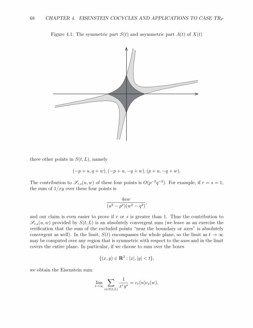
68 CHAPTER 4. EISENSTEIN COCYCLES AND APPLICATIONS TO CASE TRP
Figure 4.1: The symmetric part S(t) and asymmetric part A(t) of X(t)
three other points in S(t, L), namely
(−p+ u, q + w), (−p+ u,−q + w), (p+ u,−q + w).
The contribution to Sr,s(u,w) of these four points is O(p−2q−2). For example, if r = s = 1,the sum of 1/xy over these four points is
4uw
(u2 − p2)(w2 − q2),
and our claim is even easier to prove if r or s is greater than 1. Thus the contribution toSr,s(u,w) provided by S(t, L) is an absolutely convergent sum (we leave as an exercise theverification that the sum of the excluded points “near the boundary or axes” is absolutelyconvergent as well). In the limit, S(t) encompasses the whole plane, so the limit as t → ∞may be computed over any region that is symmetric with respect to the axes and in the limitcovers the entire plane. In particular, if we choose to sum over the boxes
(x, y) ∈ R2 : |x|, |y| < t,
we obtain the Eisenstein sum:
limt→∞
∑z∈S(t,L)
1
xrys= cr(u)cs(w),

4.2. SCZECH’S CONSTRUCTION OF THE EISENSTEIN COCYCLE 69
where cr are the periodic functions8
cr(u) := limN→∞
N∑′
k=−N
1
(k + u)r.
It remains to deal with the sum over A(t, L). Let us first treat the case r = s = 1. Wehave ∑
(x,y)∈A(t,L)
1
xy=
1
t2
∑(x,y)∈A(1, 1
tL)
1
xy.
Interpreting the right side as a Riemann sum, we recognize the limit as t→∞ as the integral
IQ :=
∫A(1)
dxdy
xy. (4.64)
The key point in this argument is that the improper integral IQ converges absolutely (ex-ercise), whereas the same is not true for the integral over X(1); this explains the need toextract the symmetric region S(t) from X(t).
A key component of Sczech’s thesis is the determination of the integral IQ. Incredibly,the integral always has the value 0, π2, or −π2, depending on Q.9 For our purposes, we willnot need the exact value of IQ, but only the fact that it depends only on Q and not on thepair (u,w). We have shown that
S1,1(u,w,Q) = c1(u)c1(w) + IQ. (4.65)
If (r, s) 6= (1, 1), then a similar argument applies, but we must be careful to deal with thefact that the integral
∫A(1)
dxdy/(xrys) does not converge because of the singularities on the
axes. We fix an ε > 0 and let
Aε(t) := (x, y) ∈ A(t) : |x| ≤ εt or |y| ≤ εt.
An elementary estimate shows that
limt→∞
∑(x,y)∈Aε(t,L)
1
xrys= 0
if (r, s) 6= (1, 1). On the complementary region A′ε(t) = A(t)− Aε(t) we have
∑(x,y)∈A′ε(t,L)
1
xrys=
1
tr+s−2
1
t2
∑(x,y)∈A′ε(1, 1tL)
1
xrys
. (4.66)
8For u 6∈ Z the cr have expressions in terms of standard trigonometric functions. For example, c1(u) =π cot(πu). We have d
ducr(u) = −rcr+1(u), hence c2(u) = π2 sin−2(πu). For u ∈ Z, we have cr(Z) = 0 for rodd and cr(Z) = 2ζ(r) for r even.
9More precisely, factor Q(x, y) = c(αx+ y)(α′x+ y). Then IQ = (sgn(α) + sgn(α′)) · π2/4.

70 CHAPTER 4. EISENSTEIN COCYCLES AND APPLICATIONS TO CASE TRP
Figure 4.2: Excising the portion of A(t) within εt of the axes
The sum in parenthesis can again be recognized as a Riemann sum whose limit as t→∞ isthe convergent integral
∫A′ε(1)
dxdy/(xrys). The extra factor 1/tr+s−2 causes the value (4.66)
to vanish as t→∞ when (r, s) 6= (1, 1). Therefore for (r, s) 6= (1, 1), we have
Sr,s(u,w,Q) = cr(u)cs(w). (4.67)
The desired result (4.62) now follows from (4.63), (4.65), and (4.67) using the Fourierexpansion (4.6) of the periodic Bernoulli polynomials. Note in particular that in the case(r, s) = (1, 1), the terms involving IQ cancel in the sum over all i, j in (4.63), since (a, b) 6∈NZ2, i.e. since v 6= 0 in (Q/Z)2. Our calculation holds with an extra term involving IQ inthe case v = 0, r = s = 1. It is possible to make a cocycle that includes the possibilityv = 0, but the module of coefficients M must be enlarged to allow for the mild dependenceon Q caused by the term IQ. This is discussed in greater detail in Section 4.5.
4.2.4 The cocycle properties
In this section, we prove that Ψ ∈ Z1(Γ,M). The Γ-invariance property of Ψ is easy toverify.
Proposition 4.11. For γ,A1, A2 ∈ Γ, P ∈ P , v ∈ V, we have
Ψ(γA1, γA2)(P, v) = Ψ(A1, A2)(γtP, γ−1v).
Proof. The Γ-invariance property
ψ(γA1, γA2)(P, z) = ψ(A1, A2)(γtP, zγ) (4.68)
4.2. SCZECH’S CONSTRUCTION OF THE EISENSTEIN COCYCLE 71
follows directly from (4.48). The desired result now follows from the definition (4.46) andthe fact that the value of Ψ is independent of the Q used to define it (use Q(z) on the leftand Q(zγ−1) on the right).
The cocycle condition is more interesting.
Proposition 4.12. For A1, A2, A3 ∈ Γ, we have
Ψ(A1, A2)−Ψ(A1, A3) + Ψ(A2, A3) = 0.
Proof. Given fixed z ∈ Z2−0, the contribution of z to Ψ(Ai, Aj) is a constant (dependingon z but not the Ai) times ψ(Ai, Aj)(P, z). Therefore it suffices to prove that
ψ(A1, A2)(P, z)− ψ(A1, A3)(P, z) + ψ(A2, A3)(P, z) = 0. (4.69)
We stress that it is crucial in this argument that region of the sum, namely |Q(z)| < t, isindependent of the Ai.
10
For each matrix Ai we let σi denote the first column not orthogonal to z. Equation (4.69)for P = 1 reads:
det(σ1, σ2)
〈z, σ1〉〈z, σ2〉− det(σ1, σ3)
〈z, σ1〉〈z, σ3〉+
det(σ2, σ3)
〈z, σ2〉〈z, σ3〉= 0. (4.70)
We will prove (4.70) for all z ∈ R2 such that the denominators do not vanish; equation (4.69)then holds for general P by applying the differential operator P (−∂x,−∂y) to equation (4.70),where z = (x, y). To prove equation (4.70), note that
det
(〈z, σ1〉 〈z, σ2〉 〈z, σ3〉σ1 σ2 σ3
)= 0
since the first row is a linear combination of the last two. Dividing by∏3
i=1〈z, σi〉 gives thedesired result.
We have proven that Ψ ∈ Z1(Γ,M); as mentioned before, this implies formally thatΨ` ∈ Z1(Γ0(`),M`).
4.2.5 Relationship with zeta functions
In this section, we prove that with Sczech’s definition of the Eisenstein cocycle, Siegel’sformula still holds. First we need a lemma. Let σ ∈ M2(R) have nonzero columns σ1, σ2.Let z ∈ Z2 be such that 〈z, σi〉 6= 0 for i = 1, 2. For a homogeneous polynomial P of degreed, define f(σ)(P, z) by the right side of (4.48):
f(σ)(P, z) =d∑r=0
Pr(σ) det(σ)
〈z, σ1〉r+1〈z, σ2〉d−r+1,
10Therefore, if one tries to regularize the sum defining Ψ by some other method, such as Hecke’s methodof multiplying by |denominator|s and analytically continuing to s = 0, then this proof of the cocycle relationwould need to altered in a significant way. In our setting, the Hecke summation method does produce thesame explicit formula for Ψ in terms of Dedekind sums for v ∈ V, and therefore gives a cocycle; but this isa quirk for dimension n = 2 and we do not know if this fact holds for n ≥ 3.
72 CHAPTER 4. EISENSTEIN COCYCLES AND APPLICATIONS TO CASE TRP
with the Pr(σ) as in (4.47). We mention two important features of the function f :
• The value of f is unchanged if either column of σ is scaled by a nonzero constant.
• For fixed P and z, f is a continuous function of σ on its domain in M2(R).
We now fix a real quadratic field F , integral ideals a and f, and let the notation be as inSection 4.1.3. In particular, w∗1, w∗2 is the dual basis to the oriented basis w1, w2 of a−1f.Let
W =
(w∗1 w∗1w∗2 w∗2
)∈ GL2(R),
using our fixed chosen embedding F ⊂ R. Recall the quadratic form P ∗ defined in (4.20):
P ∗(x, y) = N(a−1fd) N(xw∗1 + yw∗2).
Lemma 4.13. For every positive integer r, we have
f(W )(P r−1, z) =((r − 1)!)2 Nfr−1Dr−1/2
P ∗(z)r.
Proof. It is easy to verify that P ((x, y)W t) = xy · Na. Hence P r−1j (W ) = 0 for j 6= r − 1,
and P r−1r−1 (W ) = ((r− 1)!)2 Nar−1 by (4.47). The result follows from the definition of P ∗ and
the fact that det(W ) = Naf−1/√D.
The following is Siegel’s formula using Sczech’s definition of the Eisenstein cocycle.
Theorem 4.14. Let γ, P and v be defined as in (4.16), (4.17) and (4.18). For any positiveinteger r, we have
ζK/F,R(σa, 1− r) = Ψ(1, γ)(P r−1, v).
Proof. In view of the proof of Theorem 4.1 (and maintaining the notation there), we mustprove the analogue of equations (4.21)–(4.22) for the cocycle Ψ, namely
(2πi)2rΨ(1, γ)(P r−1, v) = Nfr−1Dr−1/2((r − 1)!)2ζ(P ∗, γ∗, v, r). (4.71)
Here the right side was defined in (4.23) for r > 2 and in (4.25) for r = 1.Now
(2πi)2rΨ(1, γ)(P r−1, v) = limt→∞
∑′
z∈Z2
|Q(z)|<t
ψ(1, γ)(P r−1, z)e(〈z, v〉). (4.72)
Let us choose Q = P ∗ in this limit; this choice implies that the region |Q(z)| < t is preservedunder the right action of γ on the row vectors R2. Furthermore, since γv ≡ v (mod Z2),the value of e(〈z, v〉) is preserved under this action. We therefore let Dt denote a set ofrepresentatives for the right action of γ on z ∈ Z2 − 0 : |P ∗(z)| < t, and write the sumin (4.72) as ∑
z∈Dt
e(〈z, v〉)∞∑
k=−∞
ψ(1, γ)(P r−1, zγk). (4.73)
4.3. INTEGRALITY OF THE `-SMOOTHED COCYCLE Ψ` 73
Using the cocycle properties (4.68) and (4.69) of ψ and the fact that γtP = P , the innersum in (4.73) can be recognized as the limit as N →∞ of a telescoping sum:
N∑k=−N+1
ψ(1, γ)(P r−1, zγk) =N∑
k=−N+1
ψ(γ−k, γ−k+1)((γ−k)tP r−1, z)
=N∑
k=−N+1
ψ(γ−k, γ−k+1)(P r−1, z)
= ψ(γ−N , γN)(P, z). (4.74)
Let τn denote the first column of γn. For z fixed, it is clear that τN and τ−N are not orthogonalto z for N large enough (in fact, 〈z, τn〉 = 0 for at most one value of n). Therefore, if we letαN denote the matrix with columns (τ−N , τN), then the right side of (4.74) may be writtenf(αN)(P, z). Now we use the two properties of the function f noted earlier. One checks that
τ−N ·εN
w1
=
(w∗1w∗2
)+ε2Nw1
w1
(w∗1w∗2
), (4.75)
τN ·εN
w1
=
(w∗1w∗2
)+ε2Nw1
w1
(w∗1w∗2
). (4.76)
Since the function f is invariant under scaling of columns, we replace αN by the matrixwhose columns are given by the expressions on the right in (4.75), (4.76). By the continuityproperty of f , we see that the limit as N →∞ is simply f(W )(P, z) since 0 < ε < 1. UsingLemma 4.13, we obtain that the value of (4.73) is equal to
((r − 1)!)2 Nfr−1Dr−1/2∑z∈Dt
e(〈z, v〉)P ∗(z)r
. (4.77)
For r > 1, the sum in (4.77) converges absolutely over all z ∈ (Z2 − 0)/γ, so the limit ast→∞ is equal to ζ(P ∗, γ∗, v, r) by definition (see (4.23)). For r = 1, write ζ(P ∗, γ∗, v, 1, s)(see (4.24)) as a Dirichlet series
∑∞n=1 ann
−s. By definition of Dt, the limit as t→∞ of thesum in (4.77) is the (only conditionally convergent) sum
∑∞n=1 an; meanwhile ζ(P ∗, γ∗, v, 1)
is defined to be the value of the analytic continuation of∑∞
n=1 ann−s at s = 0. By the version
of Abel’s Theorem for Dirichlet series (see [25]), these are equal. Therefore we obtain thedesired equality (4.71) for all positive integers r. The proof now follows the remainder of theproof of Theorem 4.1.
4.3 Integrality of the `-smoothed cocycle Ψ`
In this section, we prove the integrality property stated in Theorem 4.4 for the `-smoothedcocycle Ψ`, using Szcech’s definition of Ψ. The idea of `-smoothing Sczech’s cocycle wasintroduced in [5]; the contents of the rest of this chapter (except Section 4.5.1) are drawnfrom that paper.
Recall the definition of the integral subspace H1(Γ0(`),M∨` )int given in (4.39).

74 CHAPTER 4. EISENSTEIN COCYCLES AND APPLICATIONS TO CASE TRP
Theorem 4.15. We have
〈[Ψ`], [C]〉 ∈ Z[1`]
for any [C] ∈ H1(Γ,M∨` )int.
Theorem 4.15 will be proven over the next three sections. As noted in our discussionof the modular symbol definition of Ψ` in Section 4.1.6, Theorems 4.14 and 4.15 imply theintegrality result for partial zeta functions stated in Theorem 4.6. We restate the resultbelow.
Theorem 4.16. For integers r ≥ 1, we have
ζK/F,R,T (σa, 1− r) = Ψ`(1, γ)(P r−1, v)
= 〈[Ψ`], [CP,v,r]〉 ∈ Z[1`].
4.3.1 A decomposition of the `-smoothed Dedekind sum
We will prove Theorem 4.15 using the formula for Ψ` given in Theorem 4.10 by decomposingD `r,s(ρ, v) into a sum of terms that individually share an analogous integrality property. To
this end, fix a linear map L ∈ Hom(Z2,F`) such that L(
10
), L(
01
)are nonzero. For x ∈ R2−Z2,
z ∈ F`, and positive integers r, s, define
BL,zr,s (x) := Br,s(x)− `r+s−1
∑y∈F 2
`L(y)=z
Br,s
(x+ y
`
), (4.78)
where the summation runs over all y ∈ F 2` such that L(y) = z. Note that BL,z
r,s depends onx mod `Z2 rather than mod Z2, since the summation over y is restricted. It satisfies thefollowing distribution relation for integers N relatively prime to `:
BL,Nzr,s (x) = N r+s−2
∑k∈(`Z/`NZ)2
BL,zr,s
(x+ k
N
). (4.79)
As in the previous section, consider A1, A2 ∈ Γ0(`) and let ρ denote the matrix consistingof the first columns of A1, A2. We assume that det(ρ) 6= 0 since otherwise D `
r,s(ρ, v) = 0.Recall the notation ρ` = π``
−1ρ. Let R denote the first row of ρ and define L(y) = 〈R, y〉(mod `). Our desired decomposition is:
Lemma 4.17. Let x = (x1, x2) ⊂ Z2 denote a set of representatives for Z2/ρ`Z2. We
have
D `r,s(ρ, v) = sgn(det(ρ))
∑x
BL,−x1r,s (ρ−1
` (x+ π`v)). (4.80)
Remark 4.18. One easily checks that the summand in (4.80) is independent of the choiceof representative x ∈ Z2 for each class in Z2/ρ`Z
2.
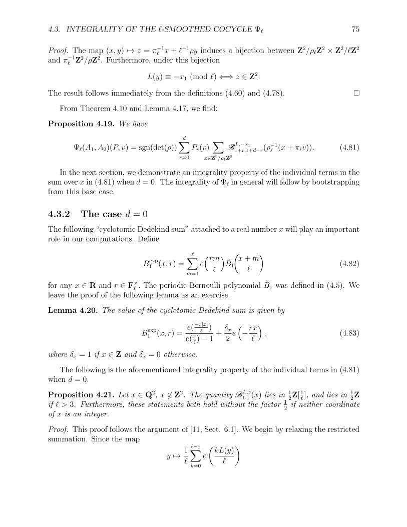
4.3. INTEGRALITY OF THE `-SMOOTHED COCYCLE Ψ` 75
Proof. The map (x, y) 7→ z = π−1` x + `−1ρy induces a bijection between Z2/ρ`Z
2 × Z2/`Z2
and π−1` Z2/ρZ2. Furthermore, under this bijection
L(y) ≡ −x1 (mod `)⇐⇒ z ∈ Z2.
The result follows immediately from the definitions (4.60) and (4.78).
From Theorem 4.10 and Lemma 4.17, we find:
Proposition 4.19. We have
Ψ`(A1, A2)(P, v) = sgn(det(ρ))d∑r=0
Pr(ρ)∑
x∈Z2/ρ`Z2
BL,−x11+r,1+d−r(ρ
−1` (x+ π`v)). (4.81)
In the next section, we demonstrate an integrality property of the individual terms in thesum over x in (4.81) when d = 0. The integrality of Ψ` in general will follow by bootstrappingfrom this base case.
4.3.2 The case d = 0
The following “cyclotomic Dedekind sum” attached to a real number x will play an importantrole in our computations. Define
Bexp1 (x, r) =
∑m=1
e(rm`
)B1
(x+m
`
)(4.82)
for any x ∈ R and r ∈ F×` . The periodic Bernoulli polynomial B1 was defined in (4.5). Weleave the proof of the following lemma as an exercise.
Lemma 4.20. The value of the cyclotomic Dedekind sum is given by
Bexp1 (x, r) =
e(−r[x]`
)
e( r`)− 1
+δx2e(−rx`
), (4.83)
where δx = 1 if x ∈ Z and δx = 0 otherwise.
The following is the aforementioned integrality property of the individual terms in (4.81)when d = 0.
Proposition 4.21. Let x ∈ Q2, x 6∈ Z2. The quantity BL,z1,1 (x) lies in 1
2Z[1
`], and lies in 1
2Z
if ` > 3. Furthermore, these statements both hold without the factor 12
if neither coordinateof x is an integer.
Proof. This proof follows the argument of [11, Sect. 6.1]. We begin by relaxing the restrictedsummation. Since the map
y 7→ 1
`
`−1∑k=0
e
(kL(y)
`
)
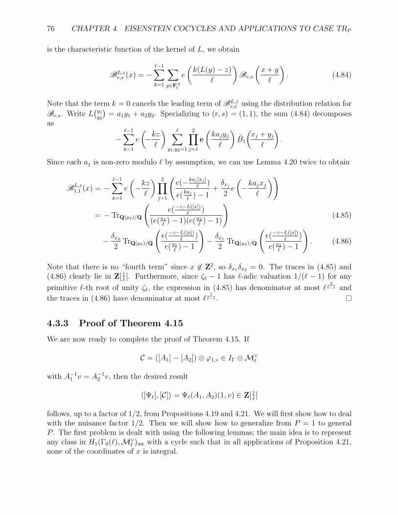
76 CHAPTER 4. EISENSTEIN COCYCLES AND APPLICATIONS TO CASE TRP
is the characteristic function of the kernel of L, we obtain
BL,zr,s (x) = −
`−1∑k=1
∑y∈F 2
`
e
(k(L(y)− z)
`
)Br,s
(x+ y
`
). (4.84)
Note that the term k = 0 cancels the leading term of BL,zr,s using the distribution relation for
Br,s. Write L(y1y2
)= a1y1 + a2y2. Specializing to (r, s) = (1, 1), the sum (4.84) decomposes
as
−`−1∑k=1
e
(−kz`
) ∑y1,y2=1
2∏j=1
e
(kajyj`
)B1
(xj + yj
`
).
Since each aj is non-zero modulo ` by assumption, we can use Lemma 4.20 twice to obtain
BL,z1,1 (x) = −
`−1∑k=1
e
(−kz`
) 2∏j=1
(e(−kaj [xj ]
`)
e(kaj`
)− 1+δxj2e
(−kajxj
`
))
= − TrQ(µ`)/Q
(e(−z−L([x])
`)
(e(a1`
)− 1)(e(a2`
)− 1)
)(4.85)
− δx22
TrQ(µ`)/Q
(e(−z−L([x])
`)
e(a1`
)− 1
)− δx1
2TrQ(µ`)/Q
(e(−z−L([x])
`)
e(a2`
)− 1
). (4.86)
Note that there is no “fourth term” since x 6∈ Z2, so δx1δx2 = 0. The traces in (4.85) and(4.86) clearly lie in Z[1
`]. Furthermore, since ζ` − 1 has `-adic valuation 1/(` − 1) for any
primitive `-th root of unity ζ`, the expression in (4.85) has denominator at most `2`−1 and
the traces in (4.86) have denominator at most `1`−1 .
4.3.3 Proof of Theorem 4.15
We are now ready to complete the proof of Theorem 4.15. If
C = ([A1]− [A2])⊗ ϕ1,v ∈ IΓ ⊗M∨`
with A−11 v = A−1
2 v, then the desired result
〈[Ψ`], [C]〉 = Ψ`(A1, A2)(1, v) ∈ Z[1`]
follows, up to a factor of 1/2, from Propositions 4.19 and 4.21. We will first show how to dealwith the nuisance factor 1/2. Then we will show how to generalize from P = 1 to generalP . The first problem is dealt with using the following lemmas; the main idea is to representany class in H1(Γ0(`),M∨
` )int with a cycle such that in all applications of Proposition 4.21,none of the coordinates of x is integral.

4.3. INTEGRALITY OF THE `-SMOOTHED COCYCLE Ψ` 77
Lemma 4.22. Any class [C] ∈ H1(Γ,M∨` )int has a representative C that can be expressed as
a linear combination of cycles of the form
([1]− [γ])⊗ ϕP,v (4.87)
satisfying conditions (4.38) and (4.39), and such that π`v ∈ V has neither coordinate integral.
Proof. By definition, a class [C] ∈ H1(Γ,M∨` )int has a representative C that may be expressed
as a linear combination of cycles
([A1]− [A2])⊗ ϕP,vsatisfying (4.38) and (4.39). This cycle is equivalent modulo the action of Γ0(`) to
([1]− [γ])⊗ ϕAt1P,A−11 v (4.88)
where γ = A−11 A2. The element (4.88) still satisfies (4.38) and (4.39). Let us therefore
relabel (At1P,A−11 v) as (P, v), with γ satisfing γtP = P and γ−1v = v. The lemma is proven
unless one of the coordinates of π`v is integral. To handle this situation we use a trick. Notethat for any g ∈ Γ0(`), we have
([1]− [g])⊗ ϕP,v = ([γ]− [γg])⊗ ϕP,vin (IΓ0(`) ⊗M∨
` )Γ0(`), and hence
([1]− [γ])⊗ ϕP,v = ([g]− [γg])⊗ ϕP,v= [1]− [g−1γg]⊗ ϕgtP,g−1v. (4.89)
The right side of (4.89) satisfies (4.38) and (4.39), and we will show that it is possible tochoose g such that g−1v has neither coordinate integral. We are given that v ∈ V`, so either
`v1 or v2 is not integral. If v2 is not integral, then g =
(1 01 1
)has the desired property, and
if `v1 is not integral, then g =
(1 0` 1
)has the desired property.
Lemma 4.23. Consider a cycle([1]− [γ])⊗ ϕP,v
satisfying conditions (4.38) and (4.39), and such that π`v ∈ V has neither coordinate integral.Then neither coordinate of y is integral for all y ∈ ρ−1
` (Z2 + π`v).
Here, as usual, ρ` denotes the matrix containing the first columns of the matrices 1 andπ`γπ
−1` .
Proof. If γ =
(a bc` d
), then ρ` =
(1 a0 c
). We have π`v ∈ ρ`(y)+Z2. In particular, v2 ≡ cy2
(mod Z), so y2 6∈ Z. Write γ′ =
(a b`c d
)= π`γπ
−1` . Since γ′(π`v) ≡ π`v (mod Z2), it follows
that π`v ∈ (γ′)−1ρ`(v) + Z2. Since (γ′)−1ρ` =
(d 1−c 0
), we find v2 ≡ −cy1 (mod Z), so
y1 6∈ Z.
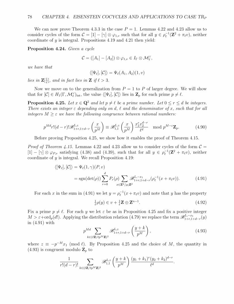
78 CHAPTER 4. EISENSTEIN COCYCLES AND APPLICATIONS TO CASE TRP
We can now prove Theorem 4.3.3 in the case P = 1. Lemmas 4.22 and 4.23 allow us toconsider cycles of the form C = [1] − [γ] ⊗ ϕ1,v such that for all y ∈ ρ−1
` (Z2 + π`v), neithercoordinate of y is integral. Propositions 4.19 and 4.21 then yield:
Proposition 4.24. Given a cycle
C = ([A1]− [A2])⊗ ϕ1,v ∈ IΓ ⊗M∨` ,
we have that〈[Ψ`], [C]〉 = Ψ`(A1, A2)(1, v)
lies in Z[1`], and in fact lies in Z if ` > 3.
Now we move on to the generalization from P = 1 to P of larger degree. We will showthat for [C] ∈ H1(Γ,M∨
` )int, the value 〈[Ψ`], [C]〉 lies in Zp for each prime p 6= `.
Proposition 4.25. Let x ∈ Q2 and let p 6= ` be a prime number. Let 0 ≤ r ≤ d be integers.There exists an integer ε depending only on d, ` and the denominator of x, such that for allintegers M ≥ ε we have the following congruence between rational numbers:
pMdr!(d− r)!BL,z1+r,1+d−r
(x
pM
)≡ BL,z
1,1
(x
pM
)xr1x
d−r2
`dmod pM−εZp. (4.90)
Before proving Proposition 4.25, we show how it enables the proof of Theorem 4.15.
Proof of Theorem 4.15. Lemmas 4.22 and 4.23 allow us to consider cycles of the form C =[1] − [γ] ⊗ ϕP,v satisfying (4.38) and (4.39), such that for all y ∈ ρ−1
` (Z2 + π`v), neithercoordinate of y is integral. We recall Proposition 4.19:
〈[Ψ`], [C]〉 = Ψ`(1, γ)(P, v)
= sgn(det(ρ))d∑r=0
Pr(ρ)∑
x∈Z2/ρ`Z2
BL,−x11+r,1+d−r(ρ
−1` (x+ π`v)). (4.91)
For each x in the sum in (4.91) we let y = ρ−1` (x+ π`v) and note that y has the property
1`ρ(y) ∈ v + 1
`Z⊕ Zn−1. (4.92)
Fix a prime p 6= `. For each y we let ε be as in Proposition 4.25 and fix a positive integerM > ε+ordp(d!). Applying the distribution relation (4.79) we replace the term BL,−x1
1+r,1+d−r(y)in (4.91) with
pMd∑
k∈(`Z/`pMZ)2
BL,z1+r,1+d−r
(y + k
pM
), (4.93)
where z ≡ −p−Mx1 (mod `). By Proposition 4.25 and the choice of M , the quantity in(4.93) is congruent modulo Zp to
1
r!(d− r)!∑
k∈(`Z/`pMZ)2
BL,z1,1
(y + k
pM
)(y1 + k1)r(y2 + k2)d−r
`d.

4.3. INTEGRALITY OF THE `-SMOOTHED COCYCLE Ψ` 79
Plugging this expression into (4.91), we note that each coefficient Pr(ρ)r!(d−r)!`d in lies in Zp, and
hence Ψ`(1, γ)(P, v) is congruent modulo Zp to
±∑x
∑k∈(`Z/`pMZ)2
BL,z1,1
(y + k
pM
) d∑r=0
Pr(σ)
r!(d− r)!· (y1 + k1)r(y2 + k2)d−r
`d. (4.94)
By the definition (4.47), the sum over r in (4.94) is equal to P(ρ(y+k)
`
), which by (4.92) and
the propertyP (v + 1
`Z⊕ Z) ⊂ Z
[1`
]given in (4.39) lies in Zp. Therefore, by Proposition 4.21, each term in (4.94) lies in Zp, andthe theorem is proven.
Proof of Proposition 4.25. As in the classical Kubota–Leopoldt construction of p-adic L-functions over Q, the proof relies on the fact that the Bernoulli polynomial Bk(x) begins
Bk(x) = xk − k
2xk−1 + · · · . (4.95)
We recall equation (4.84):
BL,z1+r,1+d−r(x) = −
`−1∑k=1
∑y∈F 2
`
e
(k(L(y)− z)
`
)B1+r,1+d−r
(x+ y
`
). (4.96)
At the expense of altering z, we may translate x by an element of pMZn and assumethat x/pM belongs to [0, 1)2. Furthermore, for each class in F 2
` we choose the representativey ∈ Z2 with 0 ≤ yj ≤ `− 1. Suppose that r ≥ 1. Equation (4.95) yields
pMrB1+r
( x1pM
+ y1
`
)≡ p−M
(x1
`
)1+r
+ (1 + r)(x1
`
)r (y1
`− 1
2
)mod pM−εZp,
where ε depends only on r, ` and the power of p in the denominator of x1. Write L(y1y2
)=
a1y1 + a2y2, and multiply the previous congruence by e(ka1y1`
). Summing over all 0 ≤ y1 ≤`− 1, the leading term of the right side vanishes and we obtain
pMr∑y1∈F`
e
(ka1y1
`
)B1+r
( x1pM
+ y1
`
)≡
(1 + r)(x1
`
)r ∑y1∈F`
e
(ka1y1
`
)B1
( x1pM
+ y1
`
)mod pM−εZp[ζ`],
(4.97)
with both sides lying in p−εZp[ζ`]. Of course, if r = 0 then this congruence holds tautolog-ically. Let us now multiply this congruence by the analogous one with r replaced by d − rand (x1, y1) by (x2, y2).
Multiplying by −e(−kz/`) and summing over k = 1, . . . , ` − 1 gives the desired resultby using (4.96) on both sides of the congruence (after dividing by (1 + r)(1 + d − r) andincreasing ε accordingly).
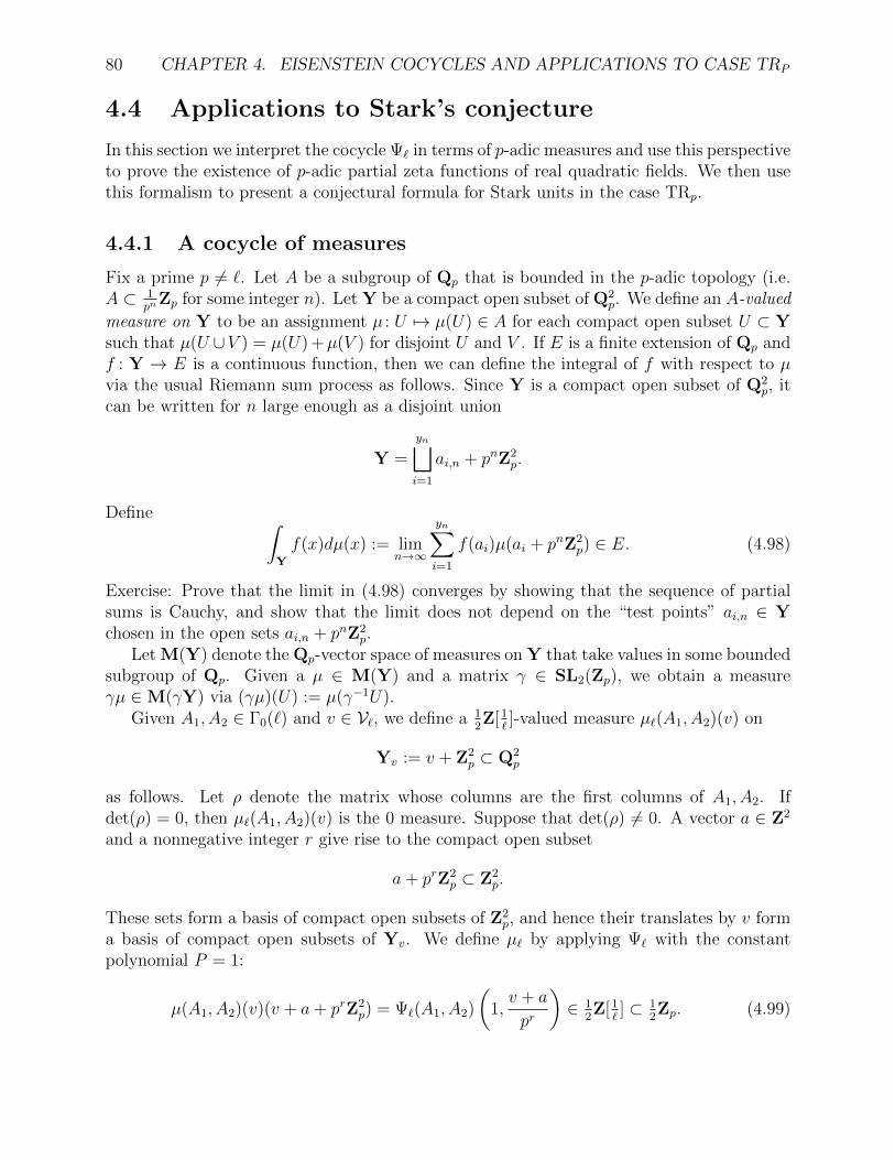
80 CHAPTER 4. EISENSTEIN COCYCLES AND APPLICATIONS TO CASE TRP
4.4 Applications to Stark’s conjecture
In this section we interpret the cocycle Ψ` in terms of p-adic measures and use this perspectiveto prove the existence of p-adic partial zeta functions of real quadratic fields. We then usethis formalism to present a conjectural formula for Stark units in the case TRp.
4.4.1 A cocycle of measures
Fix a prime p 6= `. Let A be a subgroup of Qp that is bounded in the p-adic topology (i.e.A ⊂ 1
pnZp for some integer n). Let Y be a compact open subset of Q2
p. We define an A-valued
measure on Y to be an assignment µ : U 7→ µ(U) ∈ A for each compact open subset U ⊂ Ysuch that µ(U ∪V ) = µ(U) +µ(V ) for disjoint U and V . If E is a finite extension of Qp andf : Y → E is a continuous function, then we can define the integral of f with respect to µvia the usual Riemann sum process as follows. Since Y is a compact open subset of Q2
p, itcan be written for n large enough as a disjoint union
Y =
yn⊔i=1
ai,n + pnZ2p.
Define ∫Y
f(x)dµ(x) := limn→∞
yn∑i=1
f(ai)µ(ai + pnZ2p) ∈ E. (4.98)
Exercise: Prove that the limit in (4.98) converges by showing that the sequence of partialsums is Cauchy, and show that the limit does not depend on the “test points” ai,n ∈ Ychosen in the open sets ai,n + pnZ2
p.Let M(Y) denote the Qp-vector space of measures on Y that take values in some bounded
subgroup of Qp. Given a µ ∈ M(Y) and a matrix γ ∈ SL2(Zp), we obtain a measureγµ ∈M(γY) via (γµ)(U) := µ(γ−1U).
Given A1, A2 ∈ Γ0(`) and v ∈ V`, we define a 12Z[1
`]-valued measure µ`(A1, A2)(v) on
Yv := v + Z2p ⊂ Q2
p
as follows. Let ρ denote the matrix whose columns are the first columns of A1, A2. Ifdet(ρ) = 0, then µ`(A1, A2)(v) is the 0 measure. Suppose that det(ρ) 6= 0. A vector a ∈ Z2
and a nonnegative integer r give rise to the compact open subset
a+ prZ2p ⊂ Z2
p.
These sets form a basis of compact open subsets of Z2p, and hence their translates by v form
a basis of compact open subsets of Yv. We define µ` by applying Ψ` with the constantpolynomial P = 1:
µ(A1, A2)(v)(v + a+ prZ2p) = Ψ`(A1, A2)
(1,v + a
pr
)∈ 1
2Z[1
`] ⊂ 1
2Zp. (4.99)
4.4. APPLICATIONS TO STARK’S CONJECTURE 81
It is easily checked that this assignment is well-defined, and that the distribution relationfor Ψ` implies the necessary additivity property for µ`.
Let M`,p denote the space of functions that assigns to each v ∈ V` a measure α(v) ∈M(Yv), such that the distribution relation∑
w∈( 1NZ/Z)2
α( vN
+ w)
= α(v)
is satisfied for each positive integer N relatively prime to p. Exercise: show that µ`(A1, A2) ∈M`,p.
Proposition 4.26. The function µ` : Γ0(`)2 →M`,p is a homogeneous 1-cocycle.
Proposition 4.26 follows directly from the fact that Ψ` is a cocycle; we leave the proofas an exercise. The following theorem shows that the cocycle Ψ` can be recovered from thecocycle of measures µ`; in other words, the cocycle Ψ` specialized to P = 1 determines itsvalue on all P ∈ P .
Theorem 4.27. For any P ∈ P we have
Ψ`(A1, A2)(P, v) =
∫Yv
P (x) dµ`(A1, A2)(v)(x). (4.100)
Proof. It suffices to prove the result when P is homogeneous of degree d. We follow closelythe proof of Theorem 4.15. It was shown there (see (4.94)) that there exists an integer εsuch that for each positive integer M ≥ ε, the quantity Ψ`(A1, A2)(P, v) is congruent to
±∑x
∑k∈(`Z/`pMZ)2
BL,−p−Mx11,1
(y + k
pM
)P
(ρ(y + k)
`
)(4.101)
modulo pM−εZp. Here x sums over representatives in Z2 for Z2/ρ`Z2 and y = ρ−1
` x+ ρ−1`v.The ± sign is sgn(det(ρ)). The expression (4.101) is simplified with a change of variables.Let j run over arbitrary representatives for Z2/pMZ2 (i.e. not necessarily divisible by `) suchthat j ≡ k (mod pM), and let u = x+ ρ`(j); the expression (4.101) is congruent modulo pM
to:
±∑
u∈Z2/pMρ`Z2
BL,−p−Mu11,1
(ρ−1` (u) + σ−1`v
pM
)P (π−1
` u+ v). (4.102)
Let us meanwhile evaluate the Riemann sums approximating the integral on the rightside of (4.100). There is a δ, depending on the powers of p in the denominator of P (v), suchthat for M large we have∫
Yv
P (x) dµ(x) ≡∑
j∈(Z/pMZ)2
P (v + j)µ(v + j + pMZ2p) (mod pM−δZp)
=∑
j∈(Z/pMZ)2
P (v + j)D `1,1
(ρ,v + j
pM
). (4.103)

82 CHAPTER 4. EISENSTEIN COCYCLES AND APPLICATIONS TO CASE TRP
As j runs over (Z/pMZ)2, let k run over representatives for Z2/pMZ2 such that k ≡ π`j.An argument similar to the proof of Lemma 4.17 shows that
D `1,1
(ρ,v + j
pM
)=
∑z∈Z2/ρ`Z2
BL,−z1−p−Mk1,1
(ρ−1` (z) +
ρ−1` (k) + ρ−1`v
pM
).
Substituting this expression into (4.103) and using the change of variables u = pMz+k showsthat the integral is congruent to (4.102) modulo pM−maxε,δ. Taking the limit as M → ∞,the result follows.
As before, it is convenient to express our results in terms of the natural pairings betweencohomology and homology. LetM∨
`,p denote the Zp-dual ofM`,p, which is endowed with thedual action of Γ0(`). As in Section 4.1.5, there is a natural pairing
H1(Γ0(`),M`,p)×H1(Γ0(`),M∨`,p)→ Zp
given by ⟨[µ],[∑
([A1]− [A2])⊗ ϕ]⟩
=∑
ϕ(µ(A1, A2)).
An element v ∈ V` and a continuous function f: Yv → Zp and a give rise to an elementϕf,v ∈M∨
`,p defined by
ϕf,v(α) =
∫Yv
f(x)dµ(x) where µ = α(v). (4.104)
If a polynomial P ∈ P and v ∈ V` satisfy the integrality condition (4.39), then P viewed asa continuous function on Yv has image contained in Zp. Combined with (4.104) this inducesa natural map
H1(Γ0(`),M∨` )int −→ H1(Γ0(`),M∨
`,p). (4.105)
([A1]− [A2])⊗ ϕP,v 7−→ ([A1]− [A2])⊗ ϕP,v.
Theorem 4.27 implies that for [C] ∈ H1(Γ0(`),M∨` )int, we have
〈[Ψ`], [C]〉 = 〈[µ`], [D]〉, (4.106)
where [D] denotes the image of [C] under (4.105).
4.4.2 p-adic zeta functions
We now return to the setting of a real quadratic field F . Let a be an integral ideal of Fand let c be an ideal of norm ` such that (ac, f) = 1. Let S and T be finite sets of primesof F as before, and assume that S contains all the primes of F lying above p. We will usethe p-adic measures defined above to construct the p-adic zeta functions associated to theextension K/F .
4.4. APPLICATIONS TO STARK’S CONJECTURE 83
Theorem 4.28. Fix K/F, S, T, and p as above. Let σ ∈ G = Gal(K/F ). There exists aunique Zp-valued analytic function ζK/F,S,T,p(σ, s) of the p-adic variable s ∈ W such that
ζK/F,S,T,p(σ, 1− r) = ζK/F,S,T (σ, 1− r). (4.107)
for all positive integers r.
The special values of the classical zeta function on the right side of (4.107) lie in Z[1`] ⊂ Zp
by Theorem 4.6.
Proof. First we note that it suffices to consider the case where f is divisible by all primes ofF above p. Indeed, if we let g denote the least common multiple of f and the primes dividingp, then the p-adic zeta functions for K/F and Kg/F are related as follows:
ζK/F,S,T,p(σ, s) =∑
τ∈Gal(Kg/F )
τ |K=σ
ζKg/F,S,T,p(τ, s). (4.108)
The analogous equation for the classical partial zeta functions follows from the conditionthat S contains all the primes above p.
Therefore, suppose that f is divisible by all primes of F above p. Fix a relatively prime tof and p such that σa = σ. Let P, v, and γ be as in (4.40)–(4.41). For any x ∈ Zn the quantityP (v+ x) is the norm of an integral ideal of F relatively prime to f. Since f is divisible by allthe primes above p, this quantity is an integer relatively prime to p. By the continuity of P ,we find that
P (v + x) ∈ Z×p
for all x ∈ Z2p.
We define a p-adic analytic Zp-valued function on Yv ×W :
f(x, s) = P (x)−s.
The function f in turn yields a p-adic analytic family of cycles
Ds := ([1]− [γ])⊗ ϕf(−,s),v
giving classes [Ds] ∈ H1(Γ0(`),M∨`,p).We define an analytic function ζK/F,S,T,p(σ, s) :W → Zp
by:
ζK/F,S,T,p(σ, s) = 〈[µ`], [Ds]〉 (4.109)
=
∫Yv
P (x)−sdµ(A1, A2)(v)(x). (4.110)
If r is a positive integer, then the image of CP,v,r = ([A1] − [A2]) ⊗ ϕP r−1,v under (4.105) isD1−r. Therefore, we find from (4.106):
ζK/F,S,T,p(σ, 1− r) = 〈[µ`], [D1−r]〉= 〈[Ψ`], [CP,v,r]〉= ζK/F,S,T (σ, 1− r).
This is the desired interpolation property of our p-adic zeta function.

84 CHAPTER 4. EISENSTEIN COCYCLES AND APPLICATIONS TO CASE TRP
Note that the meromorphic function ζK/F,S,p :W → Qp mentioned in (2.5) can be definedby choosing the set T = c such that c splits completely in K, and letting
ζK/F,S,p(σ, s) =ζK/F,S,T,p(σ, s)
(1− Nc1−s). (4.111)
Exercise: Show that ζK/F,S,p has the desired interpolation property (2.6) and that (4.111) isindependent of the choice of T .
4.4.3 A conjectural formula for Stark units
We finally come to the climax of our discussion of the Eisenstein cocycle—a conjecturalformula for Stark units in case TRp. Recall that K is the narrow ray class field of conductorf of F . To simplify notation, we assume that the rational prime p is inert in F , and satisfiesp ≡ 1 (mod f). This implies that p splits completely in K. The general case—in which p isreplaced by an arbitrary prime ideal p and K is replaced by its maximal subfield in which psplits—is similar, but notationally more complicated.
Denote by X := Z2p − pZ2
p the set of primitive vectors in Z2p.
Proposition 4.29. With notation as above, we have
ζK/F,S,T,p(σa, s) =
∫X
P (x)−sdµ`(1, γ)(v)(x). (4.112)
Proof. It is possible to prove this directly from our construction of ζK/F,S,T,p(σa, s) using(4.108). However, we sketch a shorter argument. Let R = S−p. Since p splits completelyin K, we have
ζK/F,S,T (σa, s) = ζK/F,R,T (σa, s)(1− p−2s) (4.113)
for s ∈ C. Let s = 1− r, with r a positive integer. We will express the zeta value in (4.113)as an integral against the measure µ using Theorems 4.16 and 4.27. Note that Yv = Z2
p
since (f, p) = 1. We have:
ζK/F,R,T (σa, s) =
∫Z2p
P (x)−sdµ`(1, γ)(v)(x) (4.114)
and
p−2sζK/F,R,T (σa, s) =
∫Z2p
P (px)−sdµ`(1, γ)(v)(x)
=
∫pZ2
p
P (x)−sdµ`(1, γ)(pv)(x)
=
∫pZ2
p
P (x)−sdµ`(1, γ)(v)(x). (4.115)

4.4. APPLICATIONS TO STARK’S CONJECTURE 85
The last equality uses the fact that pv ≡ v (mod Z2), which holds since p ≡ 1 (mod f).Combining (4.113)–(4.115) we find
ζK/F,S,T (σa, s) =
∫X
P (x)−sdµ`(1, γ)(v)(x). (4.116)
Now the left and right sides of (4.112) are continuous functions on W that agree with theleft and right sides of (4.116) on the dense set of s = 1− r, for positive integers r. Thereforethey agree as functions on W .
Note that by specializing (4.112) to s = 0, one finds that µ(1, γ)(v) has total measure 0when restricted to X:
µ(1, γ)(v)(X) = 0. (4.117)
(This is easy to prove directly as well.) Writing (4.112) using the definition of P , we have:
ζK/F,S,T,p(σa, s) = Na−s∫X
NFp/Qp(x1w1 + x2w2)−sdµ`(1, γ)(v)(x).
Taking the derivative with respect to s and evaluating at s = 0, we obtain
ζ ′K/F,S,T,p(σa, 0) = −∫X
logp NFp/Qp(x1w1 + x2w2)dµ`(1, γ)(v)(x). (4.118)
Let us fix a prime P of K above p. Gross’s Conjecture 2.3 states that the left side of (4.118)is equal to − logp NKP/Qp(u
σaT ), where uT is the Brumer–Stark–Tate unit associated to the
data (K/F, S, T, p,P):
− logp NKP/Qp(uσaT )
?= −
∫X
logp NFp/Qp(x1w1 + x2w2)dµ`(1, γ)(v)(x). (4.119)
It is natural to try to refine Gross’s conjecture by simply removing the norms from (4.119).We arrive at:
Conjecture 4.30 (Logarithmic form). We have
logp(uσaT ) =
∫X
logp(x1w1 + x2w2)dµ`(1, γ)(v)(x) ∈ OF,p.
Here OF,p denotes the p-adic completion of OF , and logp : F×p → OF,p is the Iwawasabranch of the p-adic logarithm (logp(p) = 0). The p-unit uσaT is viewed as an element of F×pvia uσaT ∈ K ⊂ KP
∼= Fp.Conjecture 4.30 is a true strengthening of Gross’s Conjecture 2.3. Whereas Gross’s
formula for uσaT has an ambiguity of multiplication by elements of norm 1 in O×F,p, Conjec-
ture 4.30 only has a finite ambiguity of the roots of unity in O×F,p. (Recall that the p-adicvaluation of uσaT is specified by the Brumer–Stark–Tate conjecture.) Gross’s conjecture is anequality in Zp, whereas Conjecture 4.30 is an equality in the quadratic unramified extensionOF,p.

86 CHAPTER 4. EISENSTEIN COCYCLES AND APPLICATIONS TO CASE TRP
We now remove the logarithms from Conjecture 4.30 in order to present an exact formulafor uσaT . Suppose that ` > 3. Using Lemma 4.22, let us assume that neither coordinate ofv ∈ V` is integral. Following the proof of Lemma 4.23 one finds that neither coordinate of yis integral for y ∈ ρ−1
` (Z2 + π`(v+apr
)) when a ∈ Z2. By Propositions 4.19 and 4.21, it followsthat
µ(1, γ)(v)(v + a+ prZ2p) = Ψ`(1, γ)
(1,v + a
pr
)∈ Z, (4.120)
i.e. µ(1, γ)(v) is a Z-valued measure on X.Let Op be the ring of integers in an extension of Qp. Given a Z-valued measure µ on X
and a continuous function f: X→ O×p , there is a multiplicative integral defined as follows:
×∫X
f(x)dµ(x) := limr→∞
∏a∈(Z/prZ)2
p-a
f(a)µ(a+prZ2p) ∈ O×p .
Here f(a) denotes the value of f at any test point in the open set a+prZ2p. The multiplicative
integral and the additive integral of (4.98) are related by the formula
logp
(×∫X
f(x)dµ(x)
)=
∫X
logp(f(x))dµ(x).
The following conjecture refines Conjecture 4.30.
Conjecture 4.31 (Multiplicative form). The element
uT (a) := pζK/F,R,T (σa,0) ×∫X
(x1w1 + x2w2)dµ`(1, γ)(v)(x) ∈ F×p (4.121)
is an element of K ⊂ KP∼= Fp. Furthermore, uT (a) ∈ Up,S,T (K), and we have the “Shimura
Reciprocity Law:”uT (a)σb = uT (ab).
Note that Conjecture 4.31 is self-contained and makes no reference to the conjectures ofBrumer–Stark–Tate or Gross. In fact, the steps we used above to motivate the statement ofConjecture 4.31 can be easily reversed to show that this conjecture implies Conjectures 1.6and 2.3, with uσaT = uT (a). We leave as an exercise the proof of the less obvious fact thatConjecture 4.31 implies Gross’s strong Conjecture 2.1 (see [11, Theorem 3.22]).
We conclude this chapter by formulating Conjecture 4.31 in terms of pairings betweencohomology and homology. Let M(X; Z) denote the Γ-module of Z-valued measures on X,and let M0(X; Z) denote the submodule of measures with total measure zero. Let C(X)denote the Γ-module of continuous functions X → O×p , and let C0(X) denote the quotientof C(X) by the subgroup of constant functions. There is a natural pairing:
M0(X; Z)× C0(X) −→ O×p (4.122)
(µ, f) 7−→ ×∫X
f(x)dµ(x).
4.5. GENERAL DEGREE 87
Let H1(Γ0(`),M`,p)int denote the subgroup generated by classes [µ] such that
µ(A1, A2)(v) ∈M0(X; Z)
whenever A1, A2 ∈ Γ0(`) and v ∈ V` satisfy
A−11 v = A−1
2 v, pv ≡ v (mod Z).
Our work above (including the application of Lemmas 4.22 and 4.23 to pass from 12Z to Z)
shows that the cohomology class [µ`] lies in H1(Γ0(`),M`,p)int.Let V`,p = v ∈ V` : pv ≡ v (mod Z2), and let N`,p denote the Γ-module of divisors on
the Γ-set C0(X)× V`,p:N`,p := Z[C0(X)× V`,p].
To be consistent with our previous notation, we denote the element corresponding to thepair (f, v) by ϕf,v. Let H1(Γ0(`),N`,p)int denote the subgroup of H1(Γ0(`),N`,p) generatedby cycles of the form ([A1]− [A2])⊗ ϕf,v, i.e. such simple tensors such that At1f = At2f andA−1
1 v = A−12 v.
The pairing (4.122) then induces a pairing:
H1(Γ0(`),M`,p)int ×H1(Γ0(`),N`,p)int −→ O×p (4.123)
([µ], ([A1]− [A2])⊗ ϕf,v) 7−→ ×∫X
f(x)dµ(A1, A2)(v)(x).
Given the setting of our real quadratic field F , it is easy to check that if
f(x1, x2) := x1w1 + x2w2,
the cycleCf,v := ([1]− [γ])⊗ ϕf,v
defines a class [Cf,v] ∈ H1(Γ0(`),N`,p)int. The main part of this verification is the observationthat γtf = ε · f , so the functions γtf and f are equal in C0(X). We then have the followingrestatement of Conjecture 4.31:
Conjecture 4.32 (Multiplicative pairing form). The element
uT (a) := pζK/F,R,T (σa,0)〈[µ`], [Cf,v]〉 ∈ F×pis an element of K ⊂ KP
∼= Fp. Furthermore, uT (a) ∈ Up,S,T (K), and we have the “ShimuraReciprocity Law:”
uT (a)σb = uT (ab).
4.5 General degree
The constructions of this chapter, from Sczech’s definition of the cocycle Ψ in Section 4.2onward, generalize to degree n ≥ 2. Furthermore, in the description above we removed0 from (Q/Z)2 in the definition of V to simplify matters. In this section we describe thegeneralization to n ≥ 2 and V := (Q/Z)n.

88 CHAPTER 4. EISENSTEIN COCYCLES AND APPLICATIONS TO CASE TRP
4.5.1 Sczech’s construction of Ψ
Let Γ = SLn(Z). For i = 1, . . . ,m, let Qi denote a linear form in n-variables with coefficientsin R that are linearly independent over Q (in particular, all the coefficients are non-zero).Let Q =
∏mi=1Qi, and let Q denote the Γ-module of such products Q, with γQ(x) := Q(xγ).
In our discussion above, we considered the case m = n = 2.For an n-tuple of matrices A = (A1, . . . , An) and an element z ∈ Zn, let σ = σ(A, z)
denote the n×n matrix whose ith column σi is the first column of the matrix Ai that is notorthogonal to z. For a polynomial P ∈ P := Q[x1, . . . , xn], let
ψ(A)(P, z) := P (−∂z1 , . . . ,−∂zn)det(σ)
〈z, σ1〉 · · · 〈z, σn〉.
If P is homogenous of degree d and v ∈ V = (Q/Z)n, define
Ψ(A)(P,Q, v) :=1
(2πi)n+dlimt→∞
∑′
z∈Zn|Q(z)|<t
ψ(A)(P, z) · e(〈z, v〉).
Sczech proved that this limit exists, but its value in general depends onQ (we saw this alreadyin the proof of Theorem 4.7 when n = 2 and v = 0). Furthermore, its value is expressible infinite terms as a Q-linear combination of generalized Dedekind sums. The dependence on Qis mild—only the signs of the coefficients of Qi(xσ
−1) enter into the formula.Next, we letM denote the Γ-module of functions P ×Q×V → Q that are distributions
in the V variable and linear in the P variable, with
(γf)(P,Q, v) := f(γtP, γ−1Q, γ−1v).
Then Ψ is a homogeneous (n− 1)-cocycle for Γ on M:
Ψ ∈ Zn−1(Γ,M).
Specializations of [Ψ] yield the classical partial zeta-values of totally real fields F of degreen at nonpositive integers. Let a, f denote integral ideals of F that are relatively prime. Letw1, . . . , wn denote a Z-basis of a−1f, and define v ∈ Qn by 1 =
∑i viwi. Define P ∈ P and
Q ∈ Q by
P (x) = NormF/Q
(n∑i=1
xiwi
), Q(x) = NormF/Q
(n∑i=1
xiw∗i
),
where w∗i is the dual basis to wi with respect to the trace. Let εin−1i=1 denote a basis
for the (free abelian) group of totally positive units of O×F congruent to 1 (mod f). There isa sign condition on the regulator of the εi to ensure compatibility with the orientation ofthe wi, as in (4.13) and (4.15). Let Ai ∈ Γ denote the matrix for multiplication by εi withrespect to the basis wj considered as a row vector. Finally, let
A =∑
π∈Sn−1
sgn(π)[(1, Aπ(1), Aπ(1)Aπ(2), . . . , Aπ(1)Aπ(2) · · ·Aπ(n−1))] ∈ Z[Γn].

4.5. GENERAL DEGREE 89
Let K be the narrow ray class extension of F associated to the conductor f, and let Rdenote the set of infinite primes of F and the primes dividing f. Sczech proves
ζK/F,R(σa, 1− r) = Ψ(A)(P r−1, Q, v) ∈ Q
for each positive integer r.
4.5.2 `-smoothing
The integrality results obtained from `-smoothing Sczech’s cocycle Ψ and applications to-wards the construction of p-adic zeta functions and Stark units is the topic of the work inprogress [5]. The basic results are sketched here.
Let Γ0(`) ⊂ Γ denote the congruence subgroup containing those matrices whose firstcolumns have every entry but the first divisible by `. Let π` denote the n × n diagonalmatrix whose first entry is ` and other diagonal entries are 1. For P homogeneous of degreed, define
Ψ`(A)(P,Q, v) = `d(Ψ(π`Aπ
−1` , π−1
` P, π`Q, π`v)− `Ψ(A,P,Q, v)).
The smoothed cocycle Ψ` satisfies the following integrality property analogous to Theo-rem 4.15:
Ψ`(A)(P,Q, v) ∈ 1
m2nZ[1
`]
if P ∈ Z[1`][x1, . . . , xn] and v satisfy
P (v + 1`Z⊕ Z) ⊂ Z[1
`].
Up to the factor m2n, which we are currently trying to eliminate using arguments such asthose in Lemmas 4.22 and 4.23, this integrality property implies Theorem 4.6 of Deligne–Ribet, Cassou–Nogues, and Barsky for the partial zeta functions of F :
ζK/F,R,T (σa, 1− r) ∈ Z[1`]
for positive integers r, where T = c for a prime of F of norm `.The arguments of Section 4.4.3 can be generalized to define a cocycle of measures µ on
the sets Yv = v + Znp . The cocycle µ can in turn be used to produce the p-adic partial zeta
functions of F as in (4.110):
ζK/F,S,T,p(σa, s) :=
∫Yv
P (x)−sdµ(A)(Q, v)(x),
where S contains all primes of F above p. Finally, we may state a conjectural formula forStark units in the general case TRp as in (4.30). For simplicity we assume that p is inert inF and that p ≡ 1 (mod f). We only present the logarithmic form of the conjecture becauseof the nuisance factor n2n (note m = n for our choice of Q) that prevents the definition ofZ-valued measures.
Conjecture 4.33. Let f(x) = x1w1 + · · ·+ xnwn. We have
logp(uσaT ) =
∫X
logp(f(x))dµ`(A)(Q, v)(x) ∈ OF,p.

90 CHAPTER 4. EISENSTEIN COCYCLES AND APPLICATIONS TO CASE TRP

Bibliography
[1] T. Arakawa, Generalized eta-functions and certain ray class invariants of realquadratic fields. Math. Ann. 260 (1982), 475–494.
[2] D. Barsky. Fonctions zeta p-adic d’une classe de rayon de nombres totalement reels.Groupe d’Etude d’Analyse Ultrametrique (5e annee: 1977/78), Exp. No. 16, 23 pp.,Secretariat Math., Paris, 1978.
[3] Pi. Cassou–Nogues. Valuers aux entiers negatifs des fonctions zeta et fonctions zetap-adique. Invent. Math. 51 (1979), no. 1, 29–59.
[4] P. Charollois, H. Darmon. Arguments des unites de Stark et periodes de seriesd’Eisenstein. (French) [Arguments for the Stark units and periods of Eisenstein series]Algebra Number Theory 2 (2008), no. 6, 655–688.
[5] P. Charollois, S. Dasgupta. An Integral Eisenstein Cocycle and Gross–Stark Unitsfor Totally Real Fields. In preparation.
[6] P. Colmez. Residu en s = 1 des fonctions zeta p-adic, Invent. Math. 91 (1988), no.2, 371–389.
[7] J. Coates, W. Sinnott. On p-adic L-functiosn over Real Quadratic Fields. Invent.Math. 25 (1974), 253–279.
[8] H. Darmon, S. Dasgupta. Elliptic Units for Real Quadratic Fields. Ann. of Math. (2)163 (2006), no. 1, 301–346.
[9] H. Darmon, S. Dasgupta, R. Pollack Hilbert modular forms and the Gross-Starkconjecture. Ann. of Math. in press.
[10] S. Dasgupta. Computations of Elliptic Units for Real Quadratic Fields. Canad. J.Math. 59 (2007), no. 3, 553–574.
[11] S. Dasgupta. Shintani Zeta Functions and Gross–Stark Units for Totally Real Fields.Duke Math. J. 143 (2008), no. 2, 225–279.
[12] P. Deligne, K. Ribet. Values of abelian L-functions at negative integers over totallyreal fields. Invent. Math. 59 (1980), no. 3, 227–286.
91
92 BIBLIOGRAPHY
[13] D. Dummit, J. Sands, B. Tangedal, Computing Stark units for totally real cubic fields.Math. Comp. 66 (1997), no. 219, 1239–1267.
[14] D. Dummit, B. Tangedal, P. van Wamelen, Stark’s conjecture over complex cubicnumber fields. Math. Comp. 73 (2004), no. 247, 1525–1546
[15] B. Gross, p-adic L-series at s = 0. J. Fac. Sci. Univ. Tokyo Sect. IA Math. 28 (1981),no. 3, 979–994 (1982).
[16] B. Gross, On the values of abelian L-functions at s = 0. J. Fac. Sci. Univ. TokyoSect. IA Math. 35 (1988), no. 1, 177–197.
[17] R. Hill, Shintani cocycles on GLn. Bull. Lond. Math. Soc. 39 (2007), no. 6, 993–1004.
[18] S. Hu, D. Solomon. Properties of higher-dimensional Shintani generating functionsand cocycles on PGL3(Q). Proc. London Math. Soc. (3) 82 (2001), no. 1, 64–88.
[19] B. Mazur. On the Arithmetic of Special Values of L-functions. Invent. Math. 55(1979), 207–240.
[20] T. Ren, R. Sczech, A refinement of Stark’s conjecture over complex cubic numberfields. J. Number Theory 129 (2009), no. 4, 831–857.
[21] J. Sands. Galois groups of exponent two and the Brumer–Stark conjecture. J. ReineAngew. Math. 349 (1984) 129–135.
[22] R. Sczech. Zur Summation von L-Reihen. (German) [On the summation of L-series]Dissertation, Rheinische Friedrich-Wilhelms-Universitat, Bonn, 1981. Bonner Math-ematische Schriften [Bonn Mathematical Publications], 141.
[23] R. Sczech. Eisenstein cocycles for GL2(Q) and values of L-functions in real quadraticfields. Comment. Math. Helv. 67 (1992), no. 3, 363–382.
[24] R. Sczech. Eisenstein Group Cocycles for GLn and values of L-functions. Invent.Math. 113 (1993), no. 3, 581–616.
[25] J. P. Serre. A Course in Arithmetic. Graduate Texts in Mathematics, No. 7. NewYork–Heidelberg, 1973.
[26] T. Shintani, On evaluation of zeta functions of totally real algebraic number fieldsat non-positive integers. J. Fac. Sci. Univ. Tokyo Sect. IA Math. 23 (1976), no. 2,393417.
[27] T. Shintani, On certain ray class invariants of real quadratic fields, Proc. JapanAcad. 53 (1977), 128–131.
[28] T. Shintani, A proof of the classical Kronecker limit formula. Tokyo J. Math. 3 (1980),191–199.

BIBLIOGRAPHY 93
[29] C. Siegel. Bernoullische Polynome und quadratische Zahlkorper. Nachr. Akad. Wiss.G ottingen Math.–Phys. Kl. II (1968), 7–38.
[30] D. Solomon, Algebraic properties of Shintani’s generating functions: Dedekind sumsand cocycles on PGL2(Q). Compositio Math. 112 (1998), no. 3, 333–362.
[31] D. Solomon, The Shintani cocycle. II. Partial zeta functions, cohomologous cocyclesand p-adic interpolation. J. Number Theory 75 (1999), no. 1, 53–108.
[32] H. Stark, L-functions at s = 1. IV. First derivatives at s = 0. Adv. in Math. 35(1980) , no. 3, 197–235.
[33] J. Tate. On Stark’s conjectures on the Behaviour of L(s, χ) at s = 0. J. Fac. Sci.Univ. Tokyo Sect. 1A Math. 28 (1981), no. 3, 963–978.
[34] A. Weil. Elliptic Functions According to Eisenstein and Kronecker. Springer–Verlag,Berlin, 1976.
[35] S. Yamamoto. On Shintani’s ray class invariant for totally real number fields, Math.Ann. 364 (2010), 449–476.