The Rationality of USDA Forecasts under

Multivariate Asymmetric Loss

Siddhartha S. Bora, Ani L. Katchova, and Todd H. Kuethe

Bora, S.S., A.L. Katchova, and T.H. Kuethe. “The Rationality of USDA Forecasts under Multivariate Asymmetric Loss.” American Journal of

Agricultural Economics (2020) https://doi.org/10.1111/ajae.12142

Siddhartha S. Bora is a Ph.D. student and Ani L. Katchova is an associate professor and

Farm Income Enhancement Chair in the Department of Agricultural, Environmental, and

Development Economics at The Ohio State University. Todd H. Kuethe is an associate

professor and the Schrader Chair in Farmland Economics in the Department of Agricultural

Economics at Purdue University.

The authors would like to thank the editor Timothy Richards and three anonymous re-

viewers for their helpful comments and suggestions and the USDA-ERS Farm Income

Team for providing us with the farm income forecast data.

Copyright 2020 by Siddhartha S. Bora, Ani L. Katchova and Todd H. Kuethe. All rights

reserved.

2

The Rationality of USDA Forecasts under Multivariate Asym-metric Loss

Abstract

A large number of previous studies suggest that many USDA forecasts are biased and/or

inefficient. These findings, however, may be the result of the assumed loss function of

USDA forecasters. We test the rationality of the USDA net cash income forecasts and the

WASDE production and price forecasts between 1988-2018 using a flexible multivariate

loss function that allows for asymmetric loss and non-separable forecast errors. Our results

provide robust evidence that USDA forecasters are rational expected loss minimizers yet

demonstrate a tendency to place a greater weight on under- or over-prediction. As a result,

this study provides an alternate interpretation of previous findings of forecast irrationality.

Key words: asymmetric loss, fixed-event forecasts, forecast rationality, net cash income,

WASDE.

JEL codes: D84, E37, Q11, Q12, Q13, Q14

1

“The U.S. Agriculture Department said on Wednesday it had pulled all staff

from an annual crop tour after an employee was threatened, and three sources

said the threat of violence was made during a phone call from an angry farmer.”

Huffstutter and Polansek (2019)

The Federal government’s statistical agencies and programs generate a large volume of

data that “the public, businesses, and governments need to make informed decisions” (Of-

fice of Management and Budget 2018, pp. 3). The U.S. Department of Agriculture (USDA)

plays an important role within the Federal government’s statistical agencies and programs.

The USDA is responsible for producing a variety of principal federal economic indicators.

Further, the USDA is home to two of the Federal government’s thirteen principal statistical

agencies, the National Agricultural Statistics Service (NASS) and the Economic Research

Service (ERS), which accounted for approximately 8% of the $3.2 billion appropriated to

primary statistical agencies in fiscal year 2017 (Office of Management and Budget 2018).

In order to provide timely information for decision-makers across the agricultural sector,

the USDA’s statistical agencies and programs provide forecasts of agricultural production,

prices, trade, uses, inventories, and farm income. The existing literature, however, suggests

that many USDA forecasts are not rational (Bailey and Brorsen 1998; Sanders and Man-

fredo 2003; Isengildina, Irwin, and Good 2006; Isengildina-Massa, MacDonald, and Xie

2012; Xiao, Hart, and Lence 2017; Kuethe, Hubbs, and Sanders 2018). The overwhelming

evidence of irrationality may lead many forecast users to question the usefulness of USDA

forecasts.

In this paper, we study the degree to which prior findings of irrationality in USDA fore-

casts can be attributed to assumptions researchers make about the costs of forecast errors,

by examining the forecaster’s loss function. The conventional practice is (i) to assume a

priori that USDA forecasts are generated to minimize a mean squared error (MSE) loss

function and (ii) to test the weak form conditions of rationality under MSE loss.1 Many

2

of the weak form conditions of forecast rationality, however, do not hold under other loss

functions (Patton and Timmermann 2007). As a result, rejections of forecast rationality

may be due to misspecified loss functions, rather than lack of rationality (Elliott, Timmer-

mann, and Komunjer 2005). Our empirical approach, by contrast, only assumes that the

forecaster’s loss function belongs to a flexible class of loss functions, of which MSE is a

special case. We then back out the parameters of the loss function that are consistent with

the observed forecasts.

As Auffhammer (2007) argues, a forecast is only optimal for a particular forecast user

when his or her loss function matches that of the forecast producer. As a result, we empiri-

cally estimate the loss functions associated with two of USDA’s most prominent forecasts

from 1988 through 2018. First, we examine USDA’s forecasts of annual net farm income

and its components. The USDA’s farm income forecasts are among the department’s most

cited statistics (McGath et al. 2009). They are closely monitored by various farm sector

stakeholders, including farm input and machinery suppliers, lenders, other farm related

industries, and state and local governments (Dubman, McElroy, and Dodson 1993). In

addition, USDA’s farm income forecasts are frequently cited in farm policy debates in

Congress and are inputs in numerous other statistical models, such as the estimation of

gross domestic production (McGath et al. 2009). Second, we examine a set of production

and price forecasts from the World Agricultural Supply and Demand Estimates (WASDE)

for three major commodities: corn, soybeans, and wheat. WASDE is an important source

of information for commodity production, consumption, trade, and prices. The existing lit-

erature provides robust evidence that WASDE releases move commodity markets (Sumner

and Mueller 1989; Fortenbery and Sumner 1993; Isengildina-Massa et al. 2008; McKenzie

2008; Adjemian 2012; Dorfman and Karali 2015; Adjemian and Irwin 2018; Karali et al.

2019; Isengildina-Massa et al. 2020a). Further, the USDA production forecasts were sub-

ject to intense scrutiny during the recent 2019 growing season. USDA’s corn acreage and

3

yield forecasts were even believed to motivate threats of violence against USDA employees

by disgruntled farmers (Huffstutter and Polansek 2019).

This study makes a number of important contributions to the literature. First, our empir-

ical approach relaxes the assumptions of MSE loss. We build on the generalized method

of moments (GMM) framework of Elliott, Timmermann, and Komunjer (2005) that jointly

estimates the forecaster’s loss function and tests for rationality of the forecasts. Elliott,

Timmermann, and Komunjer’s method is flexible as it allows for several parameteriza-

tions, as well as asymmetry in the loss function due to differential costs of over- and under-

prediction. As detailed in the next section, there are a number of reasons to believe that the

bias and inefficiencies documented in USDA forecasts may be the direct result of asym-

metric costs of over- and under-prediction.

Second, we evaluate forecasts in a multivariate framework. The overwhelming majority

of prior evaluations of USDA forecasts test rationality on each variable independently, even

though the forecasts are released as joint forecasts of several variables.2 This practice im-

plicitly assumes that the marginal costs for forecast errors in one variable are independent

of the costs for other variables or that there are no interactions between variables. Thus,

previous researchers implicitly assume separable loss functions. We instead apply the esti-

mation procedure of Komunjer and Owyang (2012) that generalizes the approach of Elliott,

Timmermann, and Komunjer (2005) to a multivariate setting with non-separable loss. Both

net farm income and WASDE are based on accounting equations, so the forecast errors of

each variable likely depend on the errors of other variables. For example, within the farm

income forecast, the costs associated with over-predicting cash receipts are compounded

when jointly under-predicting cash expenses, or within WASDE, the costs associated with

over-predicting yields are compounded when jointly over-predicting acreage.

Third, while our results are generally consistent with previous findings, our analysis

yields an alternative interpretation of the results of prior research. Batchelor (2007) draws

a distinction between a rational forecaster and a “technically” rational forecast. A rational

4

forecaster uses all available information when constructing a forecast, as in Muth (1960),

and a forecast is “technically” rational when it is unbiased and efficient, as in Diebold and

Lopez (1996). Batchelor (2007) identifies three possible explanations why rational fore-

casters may publish “technically” irrational forecasts. One, the forecaster may lack the skill

to use information efficiently and learn from forecasting errors. Two, the forecaster may

have the skill to use information efficiently, but the forecaster’s information set is insuffi-

cient. Three, the forecaster may have skill and sufficient data but responds to incentives to

make an optimistic or pessimistic forecast, namely, the forecaster responds to asymmetries

in the consequences of over- versus under-prediction. We find robust evidence that USDA

forecasts are generated to minimize an asymmetric loss function. While many USDA fore-

casts are technically irrational under traditional tests (biased and/or inefficient), this study

suggests that USDA forecasters are rational expected loss minimizers under asymmetric

loss. As Keane and Runkle (1990, pp. 719) state, “if forecasters have differential costs of

over- and under-prediction, it could be rational for them to produce biased forecasts. If we

were to find that forecasts are biased, it could still be claimed that forecasters were rational

if it could be shown that they had such differential costs.”

Background

As Elliott and Timmermann (2008, pp. 8) suggest, “no forecast is going to always be

correct, so a specification of how costly different mistakes are is needed to guide the pro-

cedure.” The loss function is a mathematical representation of the costs associated with

forecast errors, and forecasters generate projections that minimize the expected loss func-

tion. Elliott and Timmermann (2008) argue that the loss function interpretation of forecast

evaluation is valid when (i) forecasters care about the accuracy of their forecasts, and (ii)

forecasters can adjust their forecasts in a way that incorporates any costs associated with

forecast errors. The two most common loss functions employed in the existing literature

are mean squared error (MSE) and mean absolute error (MAE).

5

Forecast evaluation under MSE is particularly popular because rationality implies a num-

ber of properties that can be easily tested empirically. A rational forecast under MSE loss

is unbiased, forecast errors are serially uncorrelated, and the unconditional variance of the

forecast error is a non-decreasing function of the forecast horizon (Diebold and Lopez

1996). However, many forecasts fail to meet these conditions. Traditional tests of forecast

rationality under MSE loss suffer from the “joint hypothesis problem,” as rejection of ra-

tionality stems from either irrationality of the forecasts or a misspecified test (Fritsche et al.

2015). Thus, traditional rationality tests may be misspecified with respect to the assumed

loss function of the forecaster.

The loss function is sometimes referred to as the utility function of the forecast producer.

Kahneman and Tversky (1973) argue that forecasters may intentionally produce technically

irrational forecasts because of behavioral biases in information processing. For example,

when forecasters have a large utility of a positive outcome, they may assign greater proba-

bility weights to some values out of anticipation, hope, or greed (Weber 1994). Similarly,

when forecasters have a large disutility of a negative outcome, they may assign greater

probability weights to some values out of fear of the negative consequences associated with

underestimating probability (Weber 1994). The asymmetries in probability weights mirrors

the asymmetric reaction to gains and losses (Kahneman and Tversky 1979). Asymmetries

in the consequences of over- or under-prediction of uncertain quantities are frequently re-

ferred to as asymmetric loss functions. Weber (1994) demonstrates that asymmetric loss

functions can be derived from either an expected utility or a rank-dependent utility frame-

work.

West, Edison, and Cho (1993) argue that an asymmetric loss function is a natural can-

didate to evaluate forecasts when one seeks to emulate a utility-function-based approach

to forecast evaluation. Under asymmetric loss functions, the optimal forecast is the con-

ditional mean (MSE) or median (MAE) plus an optimal bias term (Granger 1969; Zellner

1986b; Christoffersen and Diebold 1997; Granger 1999). The size of the optimal bias will

6

depend on the parameters of the loss function (Granger 1969). In addition, the forecast

errors will not be orthogonal to variables in the forecaster’s information set (Batchelor and

Peel 1998). Patton and Timmermann (2007) assert that optimal forecasts are only unbiased

when they meet the “double symmetry” condition, in which both the variable forecasted

and the forecaster’s loss function are distributed symmetrically.

In addition to internal asymmetric costs, such as anticipation or fear, forecasters may

face external asymmetric consequences for forecast errors (Weber 1994). For example,

Laster, Bennett, and Geoum (1999) show that when forecasters are rewarded based on both

accuracy and their ability to generate publicity, their efforts to attract publicity may com-

promise forecast accuracy. In an experimental setting, Maddox and Bohil (1998) show

that people react in the appropriate direction to asymmetric payoff functions, but they are

often too conservative in their reactions. In addition to publicity, forecasters may derive

some benefit from cultivating a reputation as optimists or pessimists (Batchelor and Dua

1990). For example, when forecasters rely on others for information, optimism may help to

build relationships with information providers (Francis, Hanna, and Philbrick 1997; Fran-

cis and Philbrick 1993; Lim 2001). Similarly, forecasters may alter their predictions to

make their forecasts more attractive to particular client groups or forecast users (Batchelor

2007). While USDA forecasters may be subject to limited internal asymmetric costs, such

as anticipation or fear, they may be subject to external asymmetric consequences for fore-

cast errors, given their reliance on information from farmers and other agricultural sector

professionals, who are also USDA forecast users.

Asymmetric loss functions carry important consequences for fixed event forecasts, such

as USDA’s farm income or WASDE forecasts. Kahneman and Tversky (1973) argue that

forecasters may overweight their own past forecasts and under-react to new information.

Thus, any bias in initial forecasts will propagate forward. Batchelor (2007) demonstrates

that bias in initial forecasts will also propagate forward if forecasters face penalties for

forecast revision or are rewarded for consistency. Given that the optimal forecast under

7

asymmetric loss includes an optimal bias, any asymmetric loss early in the forecast process

may carry forward throughout later forecast revisions.

An asymmetric loss function in any one forecast may also carry important consequences

for later forecasts of other economic variables. When forecasts are made sequentially by

different agents, each published forecast becomes part of the information set of the next

forecaster. Graham (1999) demonstrates that this process of “information cascades” may

lead to herding when later forecasts are biased towards early forecasts.3 As previously

stated, USDA produces a variety of forecasts, and any asymmetries in one USDA forecast

may carry over to later USDA forecasts through information cascades. For example, if

WASDE forecasts project a significant decline in the production of a particular commodity,

this information will likely be incorporated in the USDA farm income forecasts.

Finally, the existing literature offers several explanations as to why forecasts produced

by government agencies, such as USDA, may be generated under asymmetric loss. A

number of previous studies suggest that government agency forecasts tend to be conserva-

tive or cautious (Capistran 2008; Ellison and Sargent 2012; Caunedo et al. 2018). Gov-

ernment forecasters may be cautious because stability is a crucial economic policy goal

(Capistran 2008), policy-making may require “worst case scenario” forecasts (Ellison and

Sargent 2012), or over-predicting prosperity may be worse for policymakers than under-

predicting (Caunedo et al. 2018). In addition, government forecasts may also be used to

stimulate some private sector response (Estrin and Holmes 1990). For example, Beaudry

and Willems (2018) demonstrate that overly optimistic GDP growth forecasts triggers pub-

lic and private debt accumulation. Finally, it has been argued that government agency

forecasts may be used as an instrument to justify a particular policy response (Jonung and

Larch 2006; Frankel 2011) or to put the incumbent party in a favorable light (Ulan, Dewald,

and Bullard 1995).

As previously stated, traditional forecast evaluation methods test the weak form prop-

erties of rationality under an assumed loss function, such as MSE or MAE, yet whether

8

one can conclude that bias or inefficiency represents irrationality requires knowledge of

the shape of the forecaster’s loss function (Keane and Runkle 1998). A number of studies

develop alternative loss functions that account for asymmetry (Varian 1975; Zellner 1986a;

Christoffersen and Diebold 1996; Batchelor and Peel 1998; Granger and Pesaran 2000; Ulu

2013).

Elliott, Timmermann, and Komunjer (2005), in contrast, develop an alternative forecast

evaluation framework that maintains the assumption of loss minimizing behavior and esti-

mates the shape of the loss function, or class of loss functions, that are consistent with the

observed forecasts. The method is flexible as it allows for several alternative parameteri-

zations of the loss function, with symmetry as a special case. Elliott, Timmermann, and

Komunjer’s (2005) method jointly estimates the asymmetry parameters of the forecaster’s

loss function and tests for rationality of the forecasts. Kruger and LeCrone (2019) show that

this method has a high power and is robust to fat tails, serial correlation, and outliers. The

method has been used to evaluate forecasts of a number of economic variables by profes-

sional forecasters (Aretz, Bartram, and Pope 2011; Pierdzioch, Rulke, and Stadtmann 2013;

Mamatzakis and Koutsomanoli-Filippaki 2014; Fritsche et al. 2015; Pierdzioch, Reid, and

Gupta 2016; Tsuchiya 2016a,b; Christodoulakis 2020), government agencies (Auffhammer

2007; Krol 2013; Tsuchiya 2016a; Giovannelli and Pericoli 2020), international organiza-

tions (Christodoulakis and Mamatzakis 2008; Tsuchiya 2016a; Giovannelli and Pericoli

2020), and central banks (Capistran 2008; Baghestani 2013; Pierdzioch, Rulke, and Stadt-

mann 2015; Ahn and Tsuchiya 2019; Caunedo et al. 2020). These studies overwhelmingly

suggest that forecasts that are biased or inefficient under MSE loss are rational under asym-

metric loss.

9

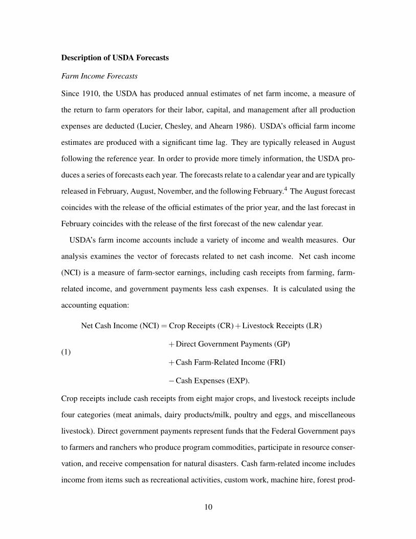
Description of USDA Forecasts

Farm Income Forecasts

Since 1910, the USDA has produced annual estimates of net farm income, a measure of

the return to farm operators for their labor, capital, and management after all production

expenses are deducted (Lucier, Chesley, and Ahearn 1986). USDA’s official farm income

estimates are produced with a significant time lag. They are typically released in August

following the reference year. In order to provide more timely information, the USDA pro-

duces a series of forecasts each year. The forecasts relate to a calendar year and are typically

released in February, August, November, and the following February.4 The August forecast

coincides with the release of the official estimates of the prior year, and the last forecast in

February coincides with the release of the first forecast of the new calendar year.

USDA’s farm income accounts include a variety of income and wealth measures. Our

analysis examines the vector of forecasts related to net cash income. Net cash income

(NCI) is a measure of farm-sector earnings, including cash receipts from farming, farm-

related income, and government payments less cash expenses. It is calculated using the

accounting equation:

(1)

Net Cash Income (NCI) = Crop Receipts (CR)+Livestock Receipts (LR)

+Direct Government Payments (GP)

+Cash Farm-Related Income (FRI)

−Cash Expenses (EXP).

Crop receipts include cash receipts from eight major crops, and livestock receipts include

four categories (meat animals, dairy products/milk, poultry and eggs, and miscellaneous

livestock). Direct government payments represent funds that the Federal Government pays

to farmers and ranchers who produce program commodities, participate in resource conser-

vation, and receive compensation for natural disasters. Cash farm-related income includes

income from items such as recreational activities, custom work, machine hire, forest prod-

10

ucts, and other farm sources. The first four items are added up to calculate gross cash

income, after which cash production expenses are subtracted to arrive at net cash income.

Since cash farm-related income forecasts are not available for most of the years and since

cash farm-related income contributes less than 10% to gross cash income, we exclude this

variable from our analysis.

McGath et al. (2009) document the economic model and estimation procedure for each

component. The forecast procedure relies on data obtained from a variety of sources, in-

cluding WASDE, Agricultural Resource Management Survey (ARMS), and NASS. While

the data sources remain constant throughout the farm income forecast process, the timing

of the release of the forecast revisions is selected to reflect changes in information. For ex-

ample, the August revision reflects updates in crop production estimates and cash receipts

from the USDA’s survey-based production and yield estimates, and the November revision

reflects updated crop production and harvest information. As time progresses, many of the

forecasted values are substituted with the official estimates. For example, by February of

next year, the WASDE acreage and yield values are final estimates, however, prices for the

marketing year remain forecasts (McGath et al. 2009).

Kuethe, Hubbs, and Sanders (2018) previously found that USDA’s bottom-line net farm

income forecasts are biased and inefficient. Specifically, initial forecasts systematically

under-predict realized values, and later forecast revisions over-react to new information.5

Isengildina-Massa et al. (2020b) extend the work of Kuethe, Hubbs, and Sanders (2018)

by examining the vector of net cash income and its components, including crop receipts,

livestock receipts, government payments, gross cash income, and cash expenditures.

Isengildina-Massa et al. (2020b) find a similar downward bias in initial net cash income

forecasts, which mainly stems from forecasts of crop receipts.

11

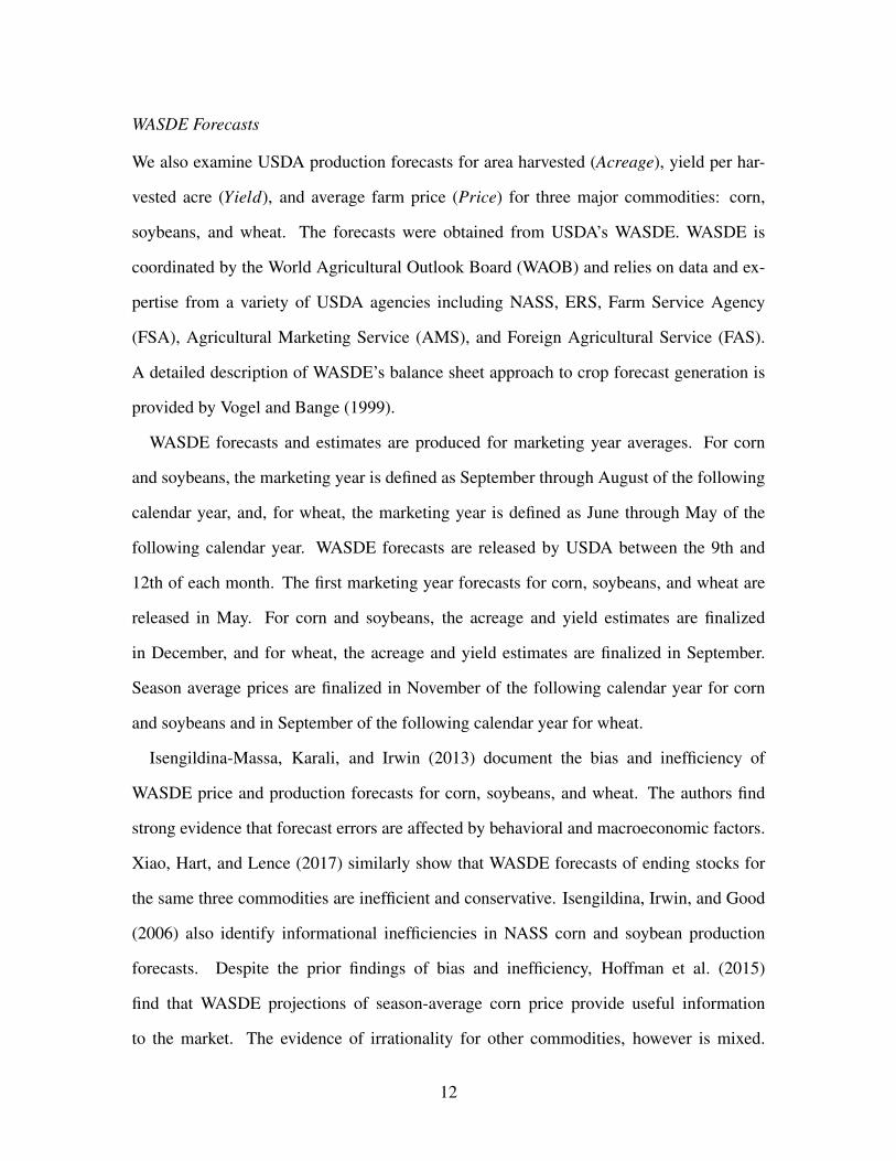
WASDE Forecasts

We also examine USDA production forecasts for area harvested (Acreage), yield per har-

vested acre (Yield), and average farm price (Price) for three major commodities: corn,

soybeans, and wheat. The forecasts were obtained from USDA’s WASDE. WASDE is

coordinated by the World Agricultural Outlook Board (WAOB) and relies on data and ex-

pertise from a variety of USDA agencies including NASS, ERS, Farm Service Agency

(FSA), Agricultural Marketing Service (AMS), and Foreign Agricultural Service (FAS).

A detailed description of WASDE’s balance sheet approach to crop forecast generation is

provided by Vogel and Bange (1999).

WASDE forecasts and estimates are produced for marketing year averages. For corn

and soybeans, the marketing year is defined as September through August of the following

calendar year, and, for wheat, the marketing year is defined as June through May of the

following calendar year. WASDE forecasts are released by USDA between the 9th and

12th of each month. The first marketing year forecasts for corn, soybeans, and wheat are

released in May. For corn and soybeans, the acreage and yield estimates are finalized

in December, and for wheat, the acreage and yield estimates are finalized in September.

Season average prices are finalized in November of the following calendar year for corn

and soybeans and in September of the following calendar year for wheat.

Isengildina-Massa, Karali, and Irwin (2013) document the bias and inefficiency of

WASDE price and production forecasts for corn, soybeans, and wheat. The authors find

strong evidence that forecast errors are affected by behavioral and macroeconomic factors.

Xiao, Hart, and Lence (2017) similarly show that WASDE forecasts of ending stocks for

the same three commodities are inefficient and conservative. Isengildina, Irwin, and Good

(2006) also identify informational inefficiencies in NASS corn and soybean production

forecasts. Despite the prior findings of bias and inefficiency, Hoffman et al. (2015)

find that WASDE projections of season-average corn price provide useful information

to the market. The evidence of irrationality for other commodities, however is mixed.

12

Isengildina-Massa, MacDonald, and Xie (2012) find evidence of bias and inefficiency in

WASDE cotton forecasts, yet Lewis and Manfredo (2012) fail to reject the rationality of

WASDE sugar production and consumption forecasts.

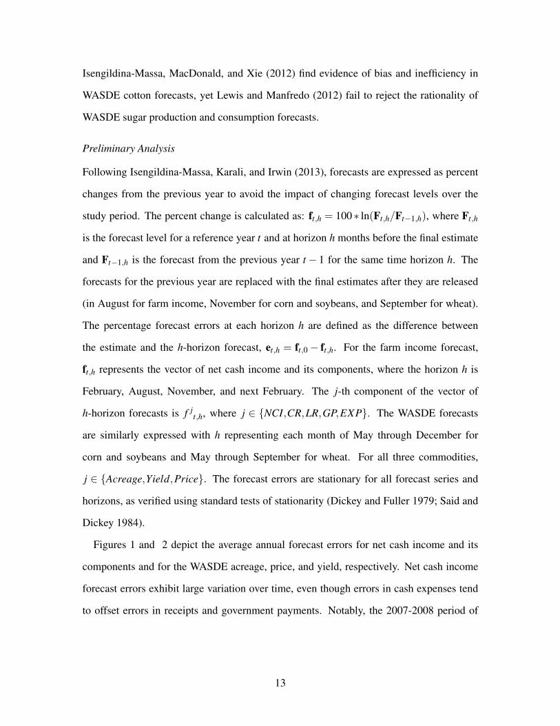
Preliminary Analysis

Following Isengildina-Massa, Karali, and Irwin (2013), forecasts are expressed as percent

changes from the previous year to avoid the impact of changing forecast levels over the

study period. The percent change is calculated as: ft,h = 100 ∗ ln(Ft,h/Ft−1,h), where Ft,h

is the forecast level for a reference year t and at horizon h months before the final estimate

and Ft−1,h is the forecast from the previous year t − 1 for the same time horizon h. The

forecasts for the previous year are replaced with the final estimates after they are released

(in August for farm income, November for corn and soybeans, and September for wheat).

The percentage forecast errors at each horizon h are defined as the difference between

the estimate and the h-horizon forecast, et,h = ft,0− ft,h. For the farm income forecast,

ft,h represents the vector of net cash income and its components, where the horizon h is

February, August, November, and next February. The j-th component of the vector of

h-horizon forecasts is f jt,h, where j ∈ {NCI,CR,LR,GP,EXP}. The WASDE forecasts

are similarly expressed with h representing each month of May through December for

corn and soybeans and May through September for wheat. For all three commodities,

j ∈ {Acreage,Yield,Price}. The forecast errors are stationary for all forecast series and

horizons, as verified using standard tests of stationarity (Dickey and Fuller 1979; Said and

Dickey 1984).

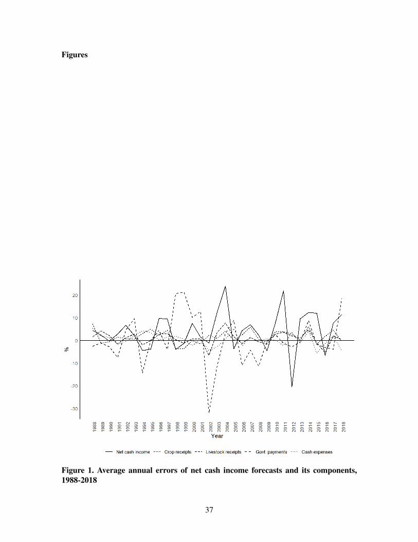
Figures 1 and 2 depict the average annual forecast errors for net cash income and its

components and for the WASDE acreage, price, and yield, respectively. Net cash income

forecast errors exhibit large variation over time, even though errors in cash expenses tend

to offset errors in receipts and government payments. Notably, the 2007-2008 period of

13

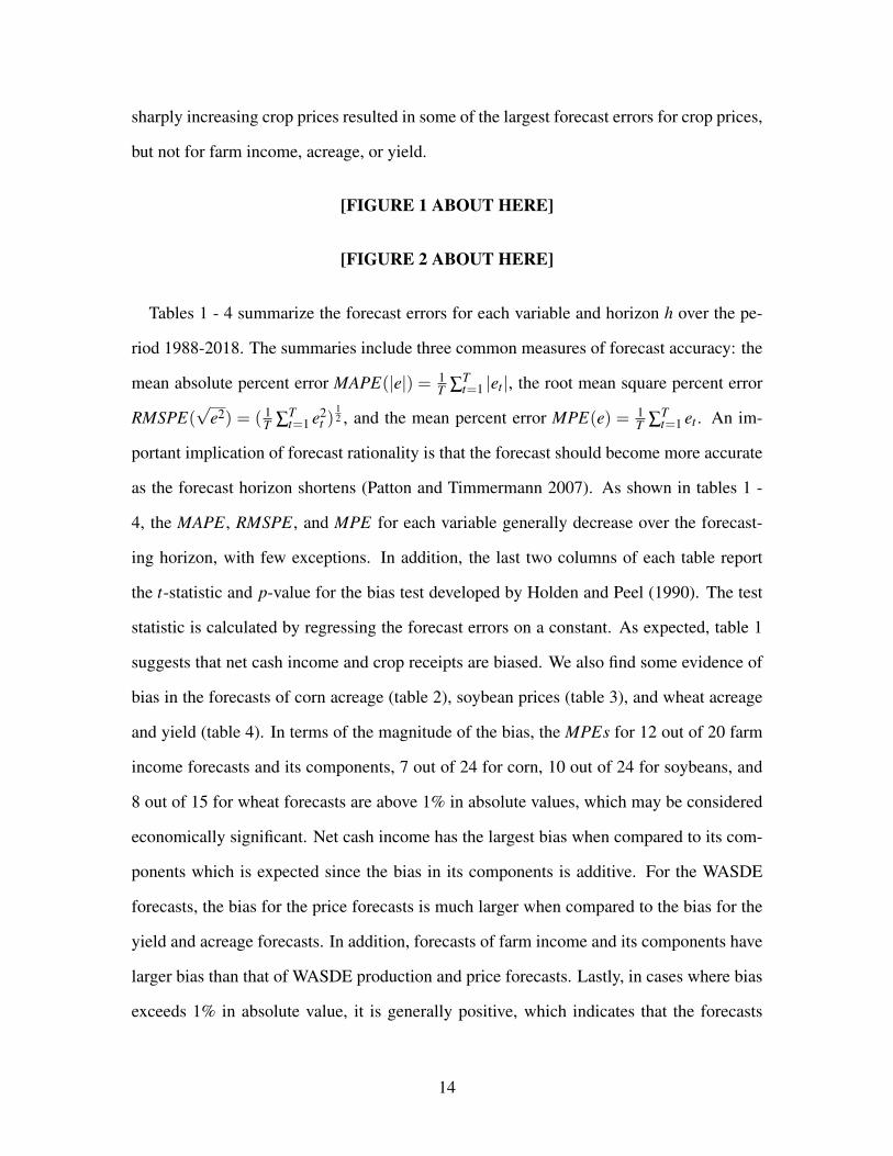
sharply increasing crop prices resulted in some of the largest forecast errors for crop prices,

but not for farm income, acreage, or yield.

[FIGURE 1 ABOUT HERE]

[FIGURE 2 ABOUT HERE]

Tables 1 - 4 summarize the forecast errors for each variable and horizon h over the pe-

riod 1988-2018. The summaries include three common measures of forecast accuracy: the

mean absolute percent error MAPE(|e|) = 1T ∑

Tt=1 |et |, the root mean square percent error

RMSPE(√

e2) = ( 1T ∑

Tt=1 e2

t )12 , and the mean percent error MPE(e) = 1

T ∑Tt=1 et . An im-

portant implication of forecast rationality is that the forecast should become more accurate

as the forecast horizon shortens (Patton and Timmermann 2007). As shown in tables 1 -

4, the MAPE, RMSPE, and MPE for each variable generally decrease over the forecast-

ing horizon, with few exceptions. In addition, the last two columns of each table report

the t-statistic and p-value for the bias test developed by Holden and Peel (1990). The test

statistic is calculated by regressing the forecast errors on a constant. As expected, table 1

suggests that net cash income and crop receipts are biased. We also find some evidence of

bias in the forecasts of corn acreage (table 2), soybean prices (table 3), and wheat acreage

and yield (table 4). In terms of the magnitude of the bias, the MPEs for 12 out of 20 farm

income forecasts and its components, 7 out of 24 for corn, 10 out of 24 for soybeans, and

8 out of 15 for wheat forecasts are above 1% in absolute values, which may be considered

economically significant. Net cash income has the largest bias when compared to its com-

ponents which is expected since the bias in its components is additive. For the WASDE

forecasts, the bias for the price forecasts is much larger when compared to the bias for the

yield and acreage forecasts. In addition, forecasts of farm income and its components have

larger bias than that of WASDE production and price forecasts. Lastly, in cases where bias

exceeds 1% in absolute value, it is generally positive, which indicates that the forecasts

14

generally under-predict realized values. These results are consistent with our later findings

that forecasters have a greater cost of over-prediction than under-prediction.

[TABLE 1 ABOUT HERE]

[TABLE 2 ABOUT HERE]

[TABLE 3 ABOUT HERE]

[TABLE 4 ABOUT HERE]

Methodology

Traditional forecast evaluation assumes that the forecaster’s objective is to minimize the

univariate mean square error (MSE) loss function:

(2) L( f jt,0, f j

t,h) = ( f jt,0− f j

t,h)2

where L(·) is the loss function, f jt,0 is the realized value of variable j for period t, and f j

t,h

is the forecast of f jt,0 conducted at a horizon of h months ahead of the realized value.

As previously stated, Elliott, Timmermann, and Komunjer (2005) develop a method for

testing forecast rationality under a flexible class of asymmetric loss functions which nest

MSE loss as a special case. Their generalized method of moments (GMM) approach jointly

estimates the asymmetry parameters of the loss function and tests for rationality. In this

study, we follow Komunjer and Owyang (2012), who develop a generalized version of the

Elliott, Timmermann, and Komunjer (2005) approach that examines multivariate forecasts

and allows for non-separable loss. We define the multivariate loss function Lp(τττ,e) as,

(3) Lp(τττ,e) =(||e||p + τττ

′e)||e||p−1

p ,

where 1≤ p < ∞, 1/p+1/q = 1, e ∈ Rn and τττ ∈Bnq = {u ∈ Rn : ||u||q < 1}. The vector

e comprises the forecast errors of n variables. The asymmetry parameter τττ determines the

15

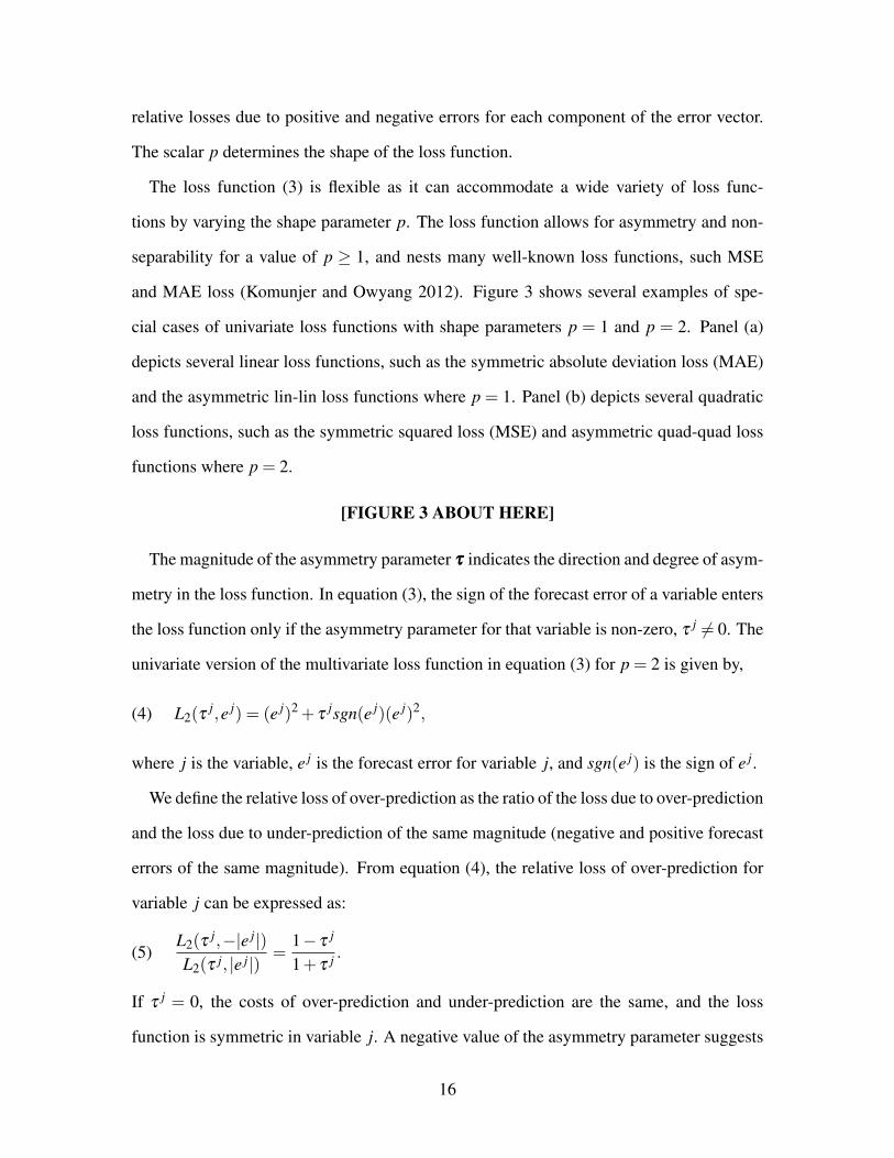
relative losses due to positive and negative errors for each component of the error vector.

The scalar p determines the shape of the loss function.

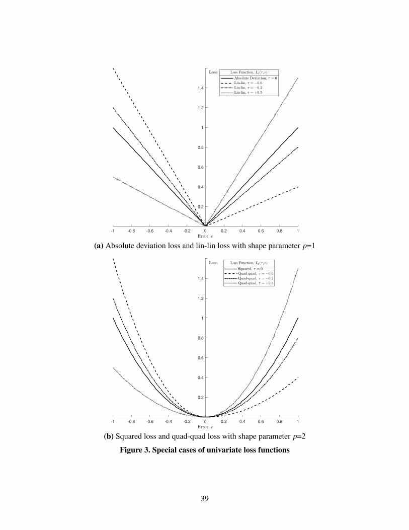
The loss function (3) is flexible as it can accommodate a wide variety of loss func-

tions by varying the shape parameter p. The loss function allows for asymmetry and non-

separability for a value of p ≥ 1, and nests many well-known loss functions, such MSE

and MAE loss (Komunjer and Owyang 2012). Figure 3 shows several examples of spe-

cial cases of univariate loss functions with shape parameters p = 1 and p = 2. Panel (a)

depicts several linear loss functions, such as the symmetric absolute deviation loss (MAE)

and the asymmetric lin-lin loss functions where p = 1. Panel (b) depicts several quadratic

loss functions, such as the symmetric squared loss (MSE) and asymmetric quad-quad loss

functions where p = 2.

[FIGURE 3 ABOUT HERE]

The magnitude of the asymmetry parameter τττ indicates the direction and degree of asym-

metry in the loss function. In equation (3), the sign of the forecast error of a variable enters

the loss function only if the asymmetry parameter for that variable is non-zero, τ j 6= 0. The

univariate version of the multivariate loss function in equation (3) for p = 2 is given by,

(4) L2(τj,e j) = (e j)2 + τ

jsgn(e j)(e j)2,

where j is the variable, e j is the forecast error for variable j, and sgn(e j) is the sign of e j.

We define the relative loss of over-prediction as the ratio of the loss due to over-prediction

and the loss due to under-prediction of the same magnitude (negative and positive forecast

errors of the same magnitude). From equation (4), the relative loss of over-prediction for

variable j can be expressed as:

(5)L2(τ

j,−|e j|)L2(τ j, |e j|)

=1− τ j

1+ τ j .

If τ j = 0, the costs of over-prediction and under-prediction are the same, and the loss

function is symmetric in variable j. A negative value of the asymmetry parameter suggests

16

that the relative loss of over-prediction is greater than one, suggesting over-predictions

are costlier than under-predictions. Figure 3 shows how the sign and magnitude of the

asymmetry parameter influence the univariate lin-lin and quad-quad loss functions.

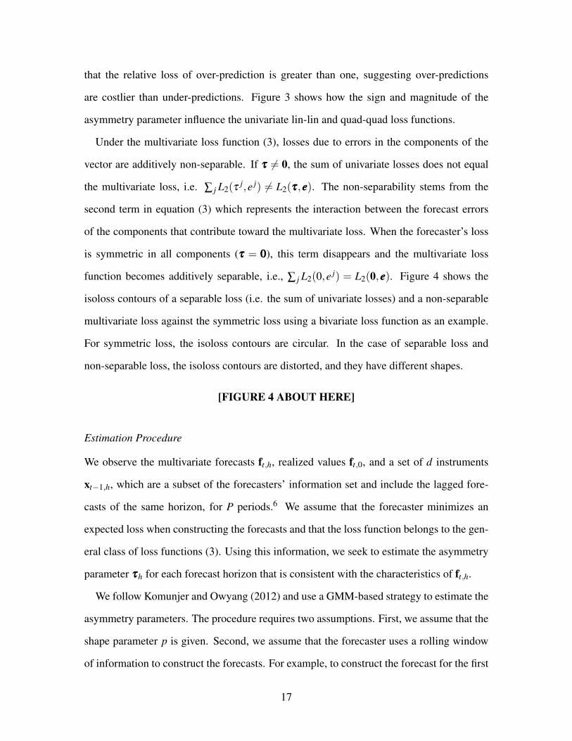
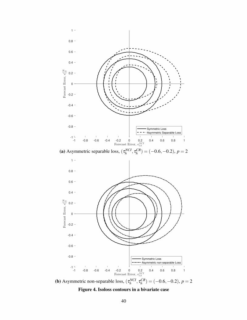
Under the multivariate loss function (3), losses due to errors in the components of the

vector are additively non-separable. If τττ 6= 0, the sum of univariate losses does not equal

the multivariate loss, i.e. ∑ j L2(τj,e j) 6= L2(τττ,eee). The non-separability stems from the

second term in equation (3) which represents the interaction between the forecast errors

of the components that contribute toward the multivariate loss. When the forecaster’s loss

is symmetric in all components (τττ = 000), this term disappears and the multivariate loss

function becomes additively separable, i.e., ∑ j L2(0,e j) = L2(0,eee). Figure 4 shows the

isoloss contours of a separable loss (i.e. the sum of univariate losses) and a non-separable

multivariate loss against the symmetric loss using a bivariate loss function as an example.

For symmetric loss, the isoloss contours are circular. In the case of separable loss and

non-separable loss, the isoloss contours are distorted, and they have different shapes.

[FIGURE 4 ABOUT HERE]

Estimation Procedure

We observe the multivariate forecasts ft,h, realized values ft,0, and a set of d instruments

xt−1,h, which are a subset of the forecasters’ information set and include the lagged fore-

casts of the same horizon, for P periods.6 We assume that the forecaster minimizes an

expected loss when constructing the forecasts and that the loss function belongs to the gen-

eral class of loss functions (3). Using this information, we seek to estimate the asymmetry

parameter τττh for each forecast horizon that is consistent with the characteristics of ft,h.

We follow Komunjer and Owyang (2012) and use a GMM-based strategy to estimate the

asymmetry parameters. The procedure requires two assumptions. First, we assume that the

shape parameter p is given. Second, we assume that the forecaster uses a rolling window

of information to construct the forecasts. For example, to construct the forecast for the first

17

period under our study, the forecaster uses information from the previous R periods. The

information window is then rolled forward to construct all forecasts until the Pth period.

Under these assumptions, the GMM estimator of the asymmetry parameter is given by,

(6) τττh = argminτττ∈Bn

q

[P−1

P

∑t=1

gp(τττ;et,h,xt−1,h)

]′× S−1×

[P−1

P

∑t=1

gp(τττ;et,h,xt−1,h)

]where,

gp(τττ;et,h,xt−1,h) = pν(et,h)+ τττ||et,h||p−1p +(p−1)τττ ′et,h||eeet,h||−1

p ν(et,h)⊗xt,h

ν(et,h) = (sgn(e j1t,h)|e

j1t,h|

p−1, . . . ,sgn(e jnt,h)|e

jnt,h|

p−1)

The optimal weight matrix S−1 is iteratively determined during the GMM estimation using

the equation,

(7) S(τττ) = P−1P

∑t=1

gp(τττ;et,h,xt−1,h)gp(τττ;et,h,xt−1,h)′

For a given shape parameter p, Komunjer and Owyang (2012) outline the conditions on

the observed errors so that the GMM estimate of the asymmetry parameter is asymptotically

normal (see Theorem 3 pp. 1072). Komunjer and Owyang (2012) also construct a J-

statistic with d > 1 instruments to test the rationality of the multivariate forecasts.

(8) Jh =

[P−1

P

∑t=1

gp(τττh;et,h,xt−1,h)

]′× S−1×

[P−1

P

∑t=1

gp(τττh;et,h,xt−1,h)

]∼ χ

2n(d−1)

A failure to reject the null hypothesis of rationality would suggest that, for a given set of

instruments, there exists some value of the asymmetry parameter for which the forecasts

are rational. Komunjer and Owyang (2012) further provide Monte Carlo evidence that the

GMM estimation under non-separable loss yields consistent estimates of the asymmetry

parameter even when the components of the vector ft,h are highly correlated. If the loss

function is misspecified as separable, it would likely produce biased estimates. Moreover,

many equations employed in USDA’s forecast models use time-lagged information from

18

several sources as inputs (Dubman, McElroy, and Dodson 1993; McGath et al. 2009; Vogel

and Bange 1999). Therefore, it is reasonable to assume that the forecaster uses a rolling

window of information to generate the forecasts. These advantages make the GMM ap-

proach well-suited for evaluating the USDA forecasts.

Robustness Checks

Our estimation procedure requires two important assumptions: the instrumental variable

set xt−1,h and the shape parameter p. To ensure that our results are not overly influenced by

these choices, we offer two important robustness checks. First, following Elliott, Timmer-

mann, and Komunjer (2005), our preferred specification uses an instrument set consisting

of a constant and one year lagged forecasts of a single variable of the same horizon (net

cash income for net cash income forecasts and average farm prices for WASDE production

forecasts). To ensure that our results are robust to the choice of instruments, we compute the

asymmetry parameters using several sets of alternative instruments that are plausibly part

of the forecaster’s information set. Second, in our preferred specification, the shape param-

eter of the loss function was fixed at p = 2, which corresponds to the well-known quadratic

loss in the univariate case. Komunjer and Owyang (2012) have shown that different values

of the shape parameter p result in consistent estimates of the asymmetry parameter. Yet,

to ensure that our results are robust to the choice of p, we estimate the model under dif-

ferent choices for the shape parameter: p = 1.5,2,2.5. Finally, our preferred specification

estimates a single asymmetry parameter over the observation period 1988 – 2018. There

may be some concern as to whether the asymmetry parameters are stable over time. The

forecast performance may change due to changes in forecasting procedures over time or un-

expected shocks, such as price disturbances, that may affect the loss function parameters.

Isengildina-Massa, Karali, and Irwin (2013), for example, showed that structural changes

in the commodity markets during the mid 2000s accounted for the largest increase in errors

in several WASDE forecasts for corn, soybeans, and wheat. Previous research suggests

19

that, if the underlying data generating process of a variable is not stable, it is rational for

error-minimizing forecasters to make serially correlated forecast revisions and systematic

forecast errors as they learn about changes in the process driving the target variable (Muth

1960; Batchelor 2007). Further, Isengildina-Massa, Karali, and Irwin (2013) demonstrate

that WASDE forecast errors grew during periods of economic growth. Higgins and Mishra

(2014) show that when forecasters are concerned with missing turning points, the forecasts

are biased downward during expansions and biased upward during recessions.

To test for the stability of the estimated loss function parameters, we use an out-

of-sample technique of detecting forecast breakdowns proposed by Giacomini and

Rossi (2009) which has been used in similar econometric settings (Mamatzakis and

Koutsomanoli-Filippaki 2014; Mamatzakis and Tsionas 2015; Christodoulakis 2020).

Following Isengildina-Massa, Karali, and Irwin (2013), we specifically examine the

potential for forecast breakdowns during the 2007-2008 commodity price boom.

Giacomini and Rossi (2009) defines forecast breakdown as a situation where the out-

of-sample performance of a forecast model is significantly inferior to its in-sample per-

formance. The method involves dividing the sample period P into in-sample and out-of-

sample windows of length m and n, where P = m+n. Then a “surprise loss” is calculated

as the difference between the out-of-sample loss and the average in-sample loss:

(9) SLt+1(τττ t) = Lt+1(τττ t)−Lt(τττ t), for t = m, . . . ,(P−1)

The average in-sample loss Lt(τττ t) is computed by first estimating the asymmetry parame-

ters τττ ttt for the in-sample window. Then the out-of-sample loss Lt+1(τττ t) is calculated using

the in-sample asymmetry parameter estimates. The test is based on the hypothesis that in

the absence of forecast breakdowns, the out-of-sample mean of the surprise losses should

be zero.

(10) H0 : E(n−1

ΣP−1t=mSLt+1(τττ t)

)= 0

20

The test statistic is calculated using a Newey-West standard error as,

(11) tm,n,1 = n1/2 SLm,n

σm,n

If the null hypothesis is rejected, a forecast breakdown is detected. We use three different

forecasting schemes which follow different assumptions about the data generating process,

(a) a fixed scheme with in-sample window t = 1, . . . ,m for all t; (b) a rolling forecasting

scheme with in-sample window t = t−m+ 1, . . . , t at time t; and (c) a recursive forecast-

ing scheme with in-sample window t = 1, . . . , t at time t. The forecast breakdown test is

performed for each of the three forecasting schemes by using the period before 2007 as the

in-sample window.

Results

The estimated asymmetry parameters for our preferred specification are presented in table

5 and figure 5 for the USDA net cash income forecasts and in table 6 and figure 6 for the

WASDE production and price forecasts for corn, soybean, and wheat. Following Komunjer

and Owyang (2012) and Caunedo et al. (2018), we use two instruments to avoid size distor-

tions in the J-test. The instrument sets used for farm income forecasts consist of a constant

and one year lagged forecasts of net cash income. For the WASDE forecasts, the instru-

ments include a constant and one year lagged forecasts of the average farm price. In each

case, the shape parameter was fixed at p = 2.

The results for the J-test for rationality under τ are presented in the bottom two rows

of tables 5 and 6. The results show that the null hypothesis of rationality could not be

rejected for any of the forecasts at the 5% significance level, for both separable and non-

separable losses. This suggests that the USDA net cash income and WASDE forecasts are

rationalizable under asymmetric loss.

Table 5 shows the GMM estimates of the asymmetry parameters for each component

of the net cash income forecast under separable and non-separable loss, along with their

21

standard errors. Figure 5 graphically presents the asymmetry parameters for net cash in-

come and its components with 95% confidence intervals under non-separable loss. While

the magnitude of τ j is generally larger in absolute terms for separable loss than for non-

separable loss, the sign and significance are mostly consistent under separable and non-

separable loss. For example, the asymmetry estimate for the February (18-month-ahead)

forecast of net cash income is –0.624 assuming separable loss, but only –0.458 under non-

separable loss. The estimates of the asymmetry parameters for crop and livestock receipts

and cash expenses are much closer to symmetric under non-separable loss, yet the asym-

metry parameters are still significantly different from zero. In contrast, the estimates are

markedly asymmetric under separable loss. These results are consistent with Komunjer

and Owyang (2012), who demonstrate that rationality could be achieved with smaller de-

gree of asymmetry under non-separable loss relative to separable loss. The pattern also

follows the empirical findings of Caunedo et al. (2018), who show that Federal Reserve’s

forecasts of growth, inflation, and unemployment are asymmetric, yet the degree of asym-

metry is less under non-separable loss. For example, the asymmetry parameter for growth

and unemployment were −0.30 and 0.32 under separable loss and −0.29 and 0.03 under

non-separable loss.

[TABLE 5 ABOUT HERE]

[TABLE 6 ABOUT HERE]

[FIGURE 5 ABOUT HERE]

Given that USDA’s net cash income forecasts are constructed using the accounting iden-

tity (1), we focus our discussion on the results under non-separable loss which is a more

realistic assumption. The relative losses associated with the asymmetry parameters are

calculated using equation (5) and presented in figure 7. The estimates of the asymmetry

parameter of net cash income are negative and significant, which suggests that USDA has

22

2.7 times higher costs associated with over-predicting 1% in the February net cash income

forecast than under-predicting it by 1%. This finding provides an alternative explanation of

the bias findings in table 1 and of previous studies’ findings that the February (18-month-

ahead) forecasts tend to under-predict net cash income and net farm income (Isengildina-

Massa et al. 2020b; Kuethe, Hubbs, and Sanders 2018). Following Granger (1969), USDA’s

initial forecasts appear biased because because over-predictions are costlier, and therefore,

the forecasts are rationally conservative. Among the components of net cash income, the

asymmetry parameter estimate is significant and negative, particularly for the February

forecast of government payments. On the other hand, the asymmetry parameter estimates

for crop and livestock receipts and production expenses are closer to zero (symmetry) even

though they are significant in most cases. These asymmetry parameters suggest that USDA

has 1.2 to 1.5 times higher costs associated with over-predicting crop and livestock receipts

and cash expenses.

[FIGURE 7 ABOUT HERE]

The estimates of asymmetry parameters generally move closer to symmetry as the ter-

minal event of releasing the USDA official estimates approaches, with the exception of

government payments (figure 5). One implication of forecast rationality is that the forecast

error should be a weakly non-decreasing function of the forecast horizon (Patton and Tim-

mermann 2007), or alternatively, that the forecasts become more accurate as the forecast

horizon reduces from say 18 months ahead to 6 months ahead of the final estimate. As a

result, a smaller degree of asymmetry is required to rationalize the forecasts as the hori-

zon reduces. Direct government payments, however, show an interesting pattern across the

forecast horizon. The asymmetry parameter is negative for the February (18-month-ahead)

forecast of government payments, suggesting over-predictions by 1% percent are 2.8 times

costlier than under-predictions by 1%. However, for the November (9-month-ahead) fore-

casts of government payments, and to some extent, for the next February (6-month-ahead)

23

forecasts, the asymmetry estimate is positive, suggesting under-predictions are costlier.

That is, before production, at the beginning of the calendar year USDA does not want to

over-predict government outlays. However, in November, after the growing season, the

USDA does not want to under-predict government program payments to farmers. This

behavior, while curious, is consistent with the bias in USDA forecasts of government pay-

ments previously reported by Isengildina-Massa et al. (2020b) and shown in table 1.

Several of the findings described above for the USDA farm income forecasts also hold

for the WASDE production and price forecasts for corn, soybeans, and wheat. The esti-

mates of the asymmetry parameters for the WASDE acreage, yield, and price forecasts are

presented in table 6 and graphically presented in figure 6 under non-separable loss, while

the separable loss results are presented in table 7. Most of the asymmetry parameters for

acreage are positive or not significant, with some negative asymmetry parameters partic-

ularly for the November and December forecasts for soybean acreage. The asymmetry

parameters for acreage are relatively small in magnitude, suggesting that although USDA

tends to over- or under-predict some acreage forecasts, the relative costs of over-predicting

are not very high. The asymmetry parameters for price, on the other hand, are mostly neg-

ative and large in magnitude. Further, the asymmetry does not appear to decrease over the

forecast horizon. In the case of corn and soybeans, the asymmetry parameters are high-

est during planting and harvest. For example, the asymmetry parameter of –0.524 for the

soybean price forecast in May shows that the relative cost of over-predicting soybean price

by 1% is 3.2 times higher than the cost of under-predicting it by 1%. Similarly, the asym-

metry parameter estimates for yield are mostly negative and significant, but they generally

move toward more symmetry over the time horizon, particularly during the last couple of

months before harvest. These findings closely correspond to the bias results shown in ta-

bles 2 – 4. Overall, these findings show that the relative costs of over-predicting prices and

yields are higher, while the relative costs of under-predicting acreage are generally higher,

particularly for wheat.

24

[FIGURE 6 ABOUT HERE]

[TABLE 7 ABOUT HERE]

Beyond our preferred specification, we also show that our findings are robust to both

the choice of shape parameter and the instrument sets used in the estimation procedure.

Through Monte Carlo simulation, Komunjer and Owyang (2012) show that different values

of the shape parameter p result in consistent estimates of the asymmetry parameter. As a

robustness check, we obtain similar results using different shape parameters. In figure 8, we

plot non-separable asymmetry estimates with shape parameter values p = 1.5 and p = 2.5

along with our preferred specification of p = 2. In both cases, the asymmetry parameter

estimates have the same sign as reported in the main results, and the magnitudes are similar,

except for government payments in the August forecasts. These estimates show that our

main results are not driven by the shape of the loss function, and the presence of asymmetry

cannot be ruled out under alternative specifications. As an additional robustness check, we

hold the shape parameter at p = 2 but vary the instruments sets. These estimates are plotted

in figure 9. The results show that the estimates of the asymmetry parameters are similar

to those reported in table 5, both in terms of sign and magnitude, except for the August

forecast of government payments.

[FIGURE 8 ABOUT HERE]

[FIGURE 9 ABOUT HERE]

The results of the structural breakdown test of Giacomini and Rossi (2009) are presented

in table 8 for the net cash income forecasts and in table 9 for the WASDE acreage, yield,

and price forecasts. Using the fixed, rolling, and recursive forecasting schemes to test

for structural breaks before and after the 2007 commodity price spikes, the test statistics

are not significant at the 5% level, with the exception of the November and December

soybean forecasts. Our interpretation is that even though crop prices sharply increased in

25

2007 resulting in high price forecast errors, the forecast errors for farm income and crop

production were not the highest in 2007 as compared to the rest of the years in our sample

(figures 1 and 2). Even though we do not find evidence of structural breakdown before

and after 2007 when considering the vector of forecasts for net cash income and WASDE

production and prices, our test does not preclude the possibility that individual asymmetry

parameters for specific components at specific time horizons may differ across sub-periods.

[TABLE 8 ABOUT HERE]

[TABLE 9 ABOUT HERE]

Conclusions

Previous studies suggest that many of the forecasts generated by the USDA are technically

irrational (biased and/or inefficient). A rejection of rationality, however, may be the result

of either the forecaster’s inefficient use of information or a misspecification of the fore-

caster’s loss function (Elliott, Timmermann, and Komunjer 2005). In this study, we jointly

estimate the parameters of USDA forecasters’ loss function and test for rationality for two

important sets of USDA forecasts: net cash income and WASDE production and price

forecasts for corn, soybeans, and wheat. Following Komunjer and Owyang (2012), the loss

function is estimated under a flexible multivariate loss function that allows for asymmetry

and non-separability in the forecast errors.

Our analysis yields two important findings. First, we find evidence of asymmetric loss

in both net cash income and WASDE forecasts. These results are consistent with previ-

ous findings of bias and inefficiency (Isengildina-Massa, Karali, and Irwin 2013; Kuethe,

Hubbs, and Sanders 2018; Isengildina-Massa et al. 2020b), yet our empirical approach

provides an alternate interpretation of these results. For example, Isengildina-Massa et al.

(2020b) find that initial USDA net cash income forecasts are downward biased. Our re-

sults suggest that a 1% over-prediction of the initial net cash income is 2.7 times as costly

26

as an under-prediction of the same percent. Thus, USDA is averse to over-predicting net

cash income at the early stages of the forecasting process. We similarly find that USDA

has a higher cost over-predicting both price and yield for corn, soybeans, and wheat. Sec-

ond, we find that under asymmetric loss, the USDA forecasters are rational expected loss

minimizers. Economic theory provides a variety of internal and external costs that may

lead otherwise rational forecasters to release “technically irrational” forecasts (Weber 1994;

Batchelor 2007).

Our findings are important for a variety of USDA forecast users, including farmers,

lenders, agricultural business leaders, and agricultural policymakers. As Auffhammer

(2007) argues, a forecast is only optimal for a particular forecast user when his or her

loss function matches that of the forecast producer. Accurately describing the loss func-

tion of USDA forecasters is therefore an important first step in forecast evaluation. Given

the important role that USDA’s farm income forecasts play in farm policy debates and

WASDE’s influence in commodity markets, the USDA should consider the internal and ex-

ternal forces that influence the cost of forecast errors. Merola and Perez (2013) argue that

government forecasting processes can be improved by increasing (i) transparency on data

reporting, (ii) accountability of forecasters, and (iii) ex ante incentives to release unbiased

forecasts. Previous research suggests that biased public forecasts can influence private de-

cision making. For example, Beaudry and Willems (2018) demonstrate that over-optimistic

GDP growth forecasts leads to higher public and private debt accumulation and later reces-

sions. Thus, our findings may also help inform future revisions of USDA forecast models

and procedures.

27

Notes1Notable exceptions include evaluations of USDA’s interval forecasts of commodity prices, including

Sanders and Manfredo (2003), Isengildina, Irwin, and Good (2004), and Isengildina-Massa and Sharp (2012).

These studies examine the proportion of actual market prices that fall in the forecasted range, or “hit rate,” of

various USDA interval forecasts. In a spirit similar to the current study, Isengildina, Irwin, and Good (2004)

examine the degree to which inaccuracy of USDA’s interval forecasts of corn and soybean price forecasts

can be attributed to inefficient use of information or the utility function of the forecasters. The authors find

evidence of the latter.

2Isengildina-Massa et al. (2020b) is one recent exception.

3Fritsche et al. (2015), conversely, identify an “anti-herding” behavior in professional forecasters where

later forecasters strategically differentiate their forecasts from those previously published.

4USDA may further revise the estimates in subsequent releases, mainly to correct errors or to incorporate

information that was not available earlier. However, to maintain consistency, we consider the first official

estimates as the realized values throughout the study, following Kuethe, Hubbs, and Sanders (2018) and

Isengildina-Massa et al. (2020b).

5Kuethe, Hubbs, and Sanders (2018) examine bottom-line net farm income which includes non-cash

income and expenses. The differences between the two measures is documented in McGath et al. (2009).

6The instrumental variables must be stationary with a full rank covariance matrix and satisfy the standard

exclusion restrictions, as outlined in Komunjer and Owyang (2012), Appendix pp. 1078-1080.

References

Adjemian, M.K. 2012. “Quantifying the WASDE announcement effect.” American Journal

of Agricultural Economics 94:238–256.

Adjemian, M.K., and S.H. Irwin. 2018. “USDA Announcement Effects in Real-Time.”

American Journal of Agricultural Economics 100:1151–1171.

Ahn, Y.B., and Y. Tsuchiya. 2019. “Asymmetric loss and the rationality of inflation fore-

casts: evidence from South Korea.” Pacific Economic Review 24:588–605.

Aretz, K., S.M. Bartram, and P.F. Pope. 2011. “Asymmetric loss functions and the rational-

ity of expected stock returns.” International Journal of Forecasting 27:413–437.

28

Auffhammer, M. 2007. “The rationality of EIA forecasts under symmetric and asymmetric

loss.” Resource and Energy Economics 29:102–121.

Baghestani, H. 2013. “Evaluating Federal Reserve predictions of growth in consumer

spending.” Applied Economics 45:1637–1646.

Bailey, D., and B.W. Brorsen. 1998. “Trends in the accuracy of USDA production forecasts

for beef and pork.” Journal of Agricultural and Resource Economics, pp. 515–525.

Batchelor, R. 2007. “Bias in macroeconomic forecasts.” International Journal of Forecast-

ing 23:189–203.

Batchelor, R., and D.A. Peel. 1998. “Rationality testing under asymmetric loss.” Economics

Letters 61:49–54.

Batchelor, R.A., and P. Dua. 1990. “Product differentiation in the economic forecasting

industry.” International Journal of Forecasting 6:311–316.

Beaudry, P., and T. Willems. 2018. “On the macroeconomic consequences of over-

optimism.” Working paper, National Bureau of Economic Research.

Capistran, C. 2008. “Bias in Federal Reserve inflation forecasts: Is the Federal Reserve

irrational or just cautious?” Journal of Monetary Economics 55:1415–1427.

Caunedo, J., R. Dicecio, I. Komunjer, and M.T. Owyang. 2020. “Asymmetry, Complemen-

tarities, and State Dependence in Federal Reserve Forecasts.” Journal of Money, Credit

and Banking 52:205–228.

Caunedo, J., R. Dicecio, I. Komunjer, and T. Owyang, Michael. 2018. “Asymmetry, Com-

plementarities, and State Dependence in Federal Reserve Forecasts.” Journal of Money,

Credit and Banking, pp. .

Christodoulakis, G. 2020. “Estimating the term structure of commodity market prefer-

ences.” European Journal of Operational Research 282:1146–1163.

Christodoulakis, G.A., and E.C. Mamatzakis. 2008. “An assessment of the EU growth fore-

casts under asymmetric preferences.” Journal of Forecasting 27:483–492.

29

Christoffersen, P.F., and F.X. Diebold. 1996. “Further results on forecasting and model

selection under asymmetric loss.” Journal of applied econometrics 11:561–571.

—. 1997. “Optimal prediction under asymmetric loss.” Econometric theory 13:808–817.

Dickey, D.A., and W.A. Fuller. 1979. “Distribution of the Estimators for Autoregressive

Time Series with a Unit Root.” Journal of the American Statistical Association 74:427–

431.

Diebold, F.X., and J.A. Lopez. 1996. “Forecast evaluation and combination.” Handbook of

Statistics 14:241–268.

Dorfman, J.H., and B. Karali. 2015. “A Nonparametric Search for Information Effects from

USDA Reports.” Journal of Agricultural and Resource Economics, pp. 124–143.

Dubman, R., R. McElroy, and C. Dodson. 1993. “Forecasting Farm Income: Documenting

USDA’s Forecast Model.” Technical Bulletin No. 1825, US Department of Agriculture,

Economic Research Service, Washington DC.

Elliott, G., and A. Timmermann. 2008. “Economic Forecasting.” Journal of Economic Lit-

erature 46:3–56.

Elliott, G., A. Timmermann, and I. Komunjer. 2005. “Estimation and Testing of Forecast

Rationality under Flexible Loss.” The Review of Economic Studies 72:1107–1125.

Ellison, M., and T.J. Sargent. 2012. “A Defense of the FOMC.” International Economic

Review 53:1047–1065.

Estrin, S., and P. Holmes. 1990. “Indicative planning in developed economies.” Journal of

Comparative Economics 14:531–554.

Fortenbery, T.R., and D. Sumner. 1993. “The effects of USDA reports in futures and options

markets.” Journal of Futures Markets 13:157–173.

Francis, J., J.D. Hanna, and D.R. Philbrick. 1997. “Management communications with

securities analysts.” Journal of Accounting and Economics 24:363–394.

Francis, J., and D. Philbrick. 1993. “Analysts’ decisions as products of a multi-task envi-

ronment.” Journal of Accounting Research 31:216–230.

30

Frankel, J. 2011. “Over-optimism in forecasts by official budget agencies and its implica-

tions.” Oxford Review of Economic Policy 27:536–562.

Fritsche, U., C. Pierdzioch, J.C. Rulke, and G. Stadtmann. 2015. “Forecasting the Brazilian

real and the Mexican peso: Asymmetric loss, forecast rationality, and forecaster herd-

ing.” International Journal of Forecasting 31:130–139.

Giacomini, R., and B. Rossi. 2009. “Detecting and Predicting Forecast Breakdowns.” The

Review of Economic Studies 76:669–705.

Giovannelli, A., and F.M. Pericoli. 2020. “Are GDP forecasts optimal? Evidence on Euro-

pean countries.” International Journal of Forecasting, pp. .

Graham, J.R. 1999. “Herding among investment newsletters: Theory and evidence.” The

Journal of Finance 54:237–268.

Granger, C.W. 1999. “Outline of forecast theory using generalized cost functions.” Spanish

Economic Review 1:161–173.

—. 1969. “Prediction with a generalized cost of error function.” Journal of the Operational

Research Society 20:199–207.

Granger, C.W.J., and M.H. Pesaran. 2000. “A decision theoretic approach to forecast evalu-

ation.” In W. Chan, W. Li, and H. Tong, eds. Statistics and finance: An interface. Imperial

College Press, pp. 261–278.

Higgins, M.L., and S. Mishra. 2014. “State dependent asymmetric loss and the consensus

forecast of real US GDP growth.” Economic Modelling 38:627–632.

Hoffman, L.A., X.L. Etienne, S.H. Irwin, E.V. Colino, and J.I. Toasa. 2015. “Forecast

performance of WASDE price projections for US corn.” Agricultural economics 46:157–

171.

Holden, K., and D.A. Peel. 1990. “On testing for unbiasedness and efficiency of forecasts.”

The Manchester School 58:120–127.

Huffstutter, P., and T. Polansek. 2019. “Farmer’s threat prompts U.S. Agriculture Depart-

ment to pull staff from crop tour.”, pp. .

31

Isengildina, O., S.H. Irwin, and D.L. Good. 2006. “Are revisions to USDA crop production

forecasts smoothed?” American Journal of Agricultural Economics 88:1091–1104.

—. 2004. “Evaluation of USDA Interval Forecasts of Corn and Soybean Prices.” American

Journal of Agricultural Economics 86:990 – 1004.

Isengildina-Massa, O., X. Cao, B. Karali, S.H. Irwin, M. Adjemian, and R.C. Johansson.

2020a. “When does usda information have the most impact on crop and livestock mar-

kets?” Journal of Commodity Markets, pp. 100137.

Isengildina-Massa, O., S.H. Irwin, D.L. Good, and J.K. Gomez. 2008. “The impact of

situation and outlook information in corn and soybean futures markets: Evidence from

WASDE reports.” Journal of Agricultural and Applied Economics 40:89–103.

Isengildina-Massa, O., B. Karali, and S.H. Irwin. 2013. “When do the USDA forecasters

make mistakes?” Applied Economics 45:5086–5103.

Isengildina-Massa, O., B. Karali, T. Kuethe, and A.L. Katchova. 2020b. “Joint Evaluation

of the System of USDA’s Farm Income Forecasts.” Applied Economic Perspectives and

Policy, pp. .

Isengildina-Massa, O., S. MacDonald, and R. Xie. 2012. “A Comprehensive Evaluation of

USDA Cotton Forecasts.” Journal of Agricultural and Resource Economics, pp. 98–113.

Isengildina-Massa, O., and J.L. Sharp. 2012. “Evaluation of USDA Interval Forecasts Re-

visited: Asymmetry and Accuracy of Corn, Soybean, and Wheat Prices.” Agribusiness

28:310–323.

Jonung, L., and M. Larch. 2006. “Improving fiscal policy in the EU: the case for indepen-

dent forecasts.” Economic Policy 21:492–534.

Kahneman, D., and A. Tversky. 1973. “On the psychology of prediction.” Psychological

review 80:237.

—. 1979. “Prospect Theory: An Analysis of Decision under Risk.” Econometrica 47:263–

292.

32

Karali, B., O. Isengildina-Massa, S.H. Irwin, M.K. Adjemian, and R. Johansson. 2019.

“Are USDA reports still news to changing crop markets?” Food Policy 84:66–76.

Keane, M.P., and D.E. Runkle. 1998. “Are financial analysts’ forecasts of corporate profits

rational?” Journal of Political Economy 106:768–805.

—. 1990. “Testing the rationality of price forecasts: New evidence from panel data.” Amer-

ican Economic Review 80:714–735.

Komunjer, I., and M.T. Owyang. 2012. “Multivariate Forecast Evaluation and Rationality

Testing.” The Review of Economics and Statistics 94:1066–1080.

Krol, R. 2013. “Evaluating state revenue forecasting under a flexible loss function.” Inter-

national Journal of Forecasting 29:282–289.

Kruger, J.J., and J. LeCrone. 2019. “Forecast Evaluation Under Asymmetric Loss: A

Monte Carlo Analysis of the EKT Method.” Oxford Bulletin of Economics and Statis-

tics 81:437–455.

Kuethe, T., T. Hubbs, and D.R. Sanders. 2018. “Evaluating the USDA’s Net Farm Income

Forecast.” Journal of Agricultural and Resource Economics 43:276505.

Laster, D., P. Bennett, and I.S. Geoum. 1999. “Rational bias in macroeconomic forecasts.”

The Quarterly Journal of Economics 114:293–318.

Lewis, K.E., and M.R. Manfredo. 2012. “An evaluation of the USDA sugar production and

consumption forecasts.” Journal of Agribusiness 30:155–172.

Lim, T. 2001. “Rationality and analysts’ forecast bias.” The journal of Finance 56:369–385.

Lucier, G., A. Chesley, and M.C. Ahearn. 1986. “Farm Income Data: A Historical Perspec-

tive.” Statistical Bulletin No. 740, US Department of Agriculture, Economic Research

Service, Washington DC.

Maddox, W.T., and C.J. Bohil. 1998. “Base-rate and payoff effects in multidimensional per-

ceptual categorization.” Journal of Experimental Psychology: Learning, Memory, and

Cognition 24:1459.

33

Mamatzakis, E., and A. Koutsomanoli-Filippaki. 2014. “Testing the rationality of DOE’s

energy price forecasts under asymmetric loss preferences.” Energy Policy 68:567–575.

Mamatzakis, E., and M.G. Tsionas. 2015. “How are market preferences shaped? The case

of sovereign debt of stressed euro-area countries.” Journal of Banking & Finance 61:106

– 116.

McGath, C., R. McElroy, R. Strickland, L. Traub, T. Covey, S. Short, J. Johnson, R. Green,

M. Ali, and S. Vogel. 2009. “Forecasting Farm Income: Documenting USDA’s Fore-

cast Model.” Technical Bulletin No. 1924, US Department of Agriculture, Economic

Research Service, Washington DC.

McKenzie, A.M. 2008. “Pre-harvest price expectations for corn: The information content

of USDA reports and new crop futures.” American Journal of Agricultural Economics

90:351–366.

Merola, R., and J.J. Perez. 2013. “Fiscal forecast errors: governments versus independent

agencies?” European Journal of Political Economy 32:285–299.

Muth, J.F. 1960. “Optimal properties of exponentially weighted forecasts.” Journal of the

american statistical association 55:299–306.

Office of Management and Budget. 2018. “Statistical programs of the United States gov-

ernment.” Annual Report, pp. .

Patton, A.J., and A. Timmermann. 2007. “Properties of optimal forecasts under asymmetric

loss and nonlinearity.” Journal of Econometrics 140:884–918.

Pierdzioch, C., M.B. Reid, and R. Gupta. 2016. “Forecasting the South African inflation

rate: On asymmetric loss and forecast rationality.” Economic Systems 40:82–92.

Pierdzioch, C., J.C. Rulke, and G. Stadtmann. 2015. “Central banks’ inflation forecasts un-

der asymmetric loss: Evidence from four Latin-American countries.” Economics Letters

129:66–70.

—. 2013. “Forecasting US housing starts under asymmetric loss.” Applied Financial Eco-

nomics 23:505–513.

34

Said, S.E., and D.A. Dickey. 1984. “Testing for Unit Roots in Autoregressive-Moving Av-

erage Models of Unknown Order.” Biometrika 71:599–607.

Sanders, D.R., and M.R. Manfredo. 2003. “USDA Livestock Price Forecasts: A Compre-

hensive Evaluation.” Journal of Agricultural and Resource Economics, pp. 19.

Sumner, D.A., and R.A. Mueller. 1989. “Are harvest forecasts news? USDA announce-

ments and futures market reactions.” American Journal of Agricultural Economics 71:1–

8.

Tsuchiya, Y. 2016a. “Assessing macroeconomic forecasts for Japan under an asymmetric

loss function.” International Journal of Forecasting 32:233–242.

—. 2016b. “Asymmetric loss and rationality of Chinese renminbi forecasts: An implication

for the trade between China and the US.” Journal of International Financial Markets,

Institutions and Money 44:116–127.

Ulan, M., W.G. Dewald, and J.B. Bullard. 1995. “US official forecasts of G-7 economies,

1976-90.” Federal Reserve Bank of St. Louis Review 77:39.

Ulu, Y. 2013. “Multivariate test for forecast rationality under asymmetric loss functions:

Recent evidence from MMS survey of inflation–output forecasts.” Economics Letters

119:168–171.

Varian, H.R. 1975. “A Bayesian approach to real estate assessment.” In S. E. Fienber and

A. Zellner, eds. Studies in Bayesian econometric and statistics in Honor of Leonard J.

Savage. Amsterdam: North Holland, pp. 195–208.

Vogel, F., and G. Bange. 1999. “Understanding USDA Crop Forecasts.” Technical Bulletin

No. 1554, US Department of Agriculture, National Agricultural Statistics Service and

Office of the Chief Economist, World Agricultural Outlook Board, Washington DC.

Weber, E.U. 1994. “From subjective probabilities to decision weights: The effect of asym-

metric loss functions on the evaluation of uncertain outcomes and events.” Psychological

Bulletin 115:228.

35

West, K.D., H.J. Edison, and D.C. Cho. 1993. “A Utility-Based Comparison of Some Mod-

els of Exchange Rate Volatility.” Journal of International Economics 35:23–45.

Xiao, J., C.E. Hart, and S.H. Lence. 2017. “USDA Forecasts Of Crop Ending Stocks: How

Well Have They Performed?” Applied Economic Perspectives and Policy 39:220–241.

Zellner, A. 1986a. “Bayesian estimation and prediction using asymmetric loss functions.”

Journal of the American Statistical Association 81:446–451.

—. 1986b. “Biased predictors, rationality and the evaluation of forecasts.” Economics Let-

ters 21:45–48.

36

Figures

Figure 1. Average annual errors of net cash income forecasts and its components,1988-2018

37

Figure 2. Average annual errors of WASDE forecasts for acreage, yield, and price,1988-2018 38

-1 -0.8 -0.6 -0.4 -0.2 0 0.2 0.4 0.6 0.8 1

0.2

0.4

0.6

0.8

1

1.2

1.4

(a) Absolute deviation loss and lin-lin loss with shape parameter p=1

-1 -0.8 -0.6 -0.4 -0.2 0 0.2 0.4 0.6 0.8 1

0.2

0.4

0.6

0.8

1

1.2

1.4

(b) Squared loss and quad-quad loss with shape parameter p=2

Figure 3. Special cases of univariate loss functions

39

-1 -0.8 -0.6 -0.4 -0.2 0 0.2 0.4 0.6 0.8 1-1

-0.8

-0.6

-0.4

-0.2

0

0.2

0.4

0.6

0.8

1

Symmetric Loss

Asymmetric Separable Loss

(a) Asymmetric separable loss, (τNCIh ,τCR

h ) = (−0.6,−0.2), p = 2

-1 -0.8 -0.6 -0.4 -0.2 0 0.2 0.4 0.6 0.8 1-1

-0.8

-0.6

-0.4

-0.2

0

0.2

0.4

0.6

0.8

1

Symmetric Loss

Asymmetric non-separable Loss

(b) Asymmetric non-separable loss, (τNCIh ,τCR

h ) = (−0.6,−0.2), p = 2

Figure 4. Isoloss contours in a bivariate case

40

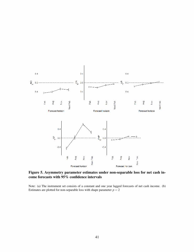
Figure 5. Asymmetry parameter estimates under non-separable loss for net cash in-come forecasts with 95% confidence intervals

Note: (a) The instrument set consists of a constant and one year lagged forecasts of net cash income. (b)Estimates are plotted for non-separable loss with shape parameter p = 2

41

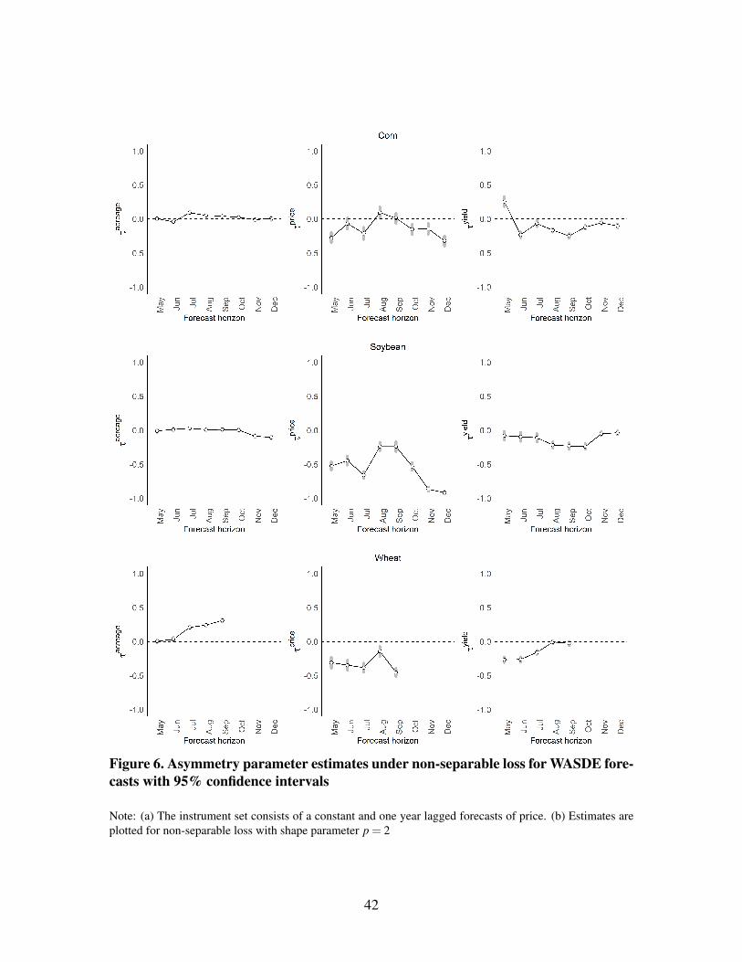
Figure 6. Asymmetry parameter estimates under non-separable loss for WASDE fore-casts with 95% confidence intervals

Note: (a) The instrument set consists of a constant and one year lagged forecasts of price. (b) Estimates areplotted for non-separable loss with shape parameter p = 2

42

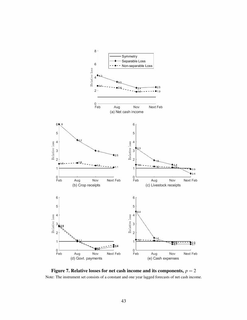
Figure 7. Relative losses for net cash income and its components, p = 2Note: The instrument set consists of a constant and one year lagged forecasts of net cash income.

43

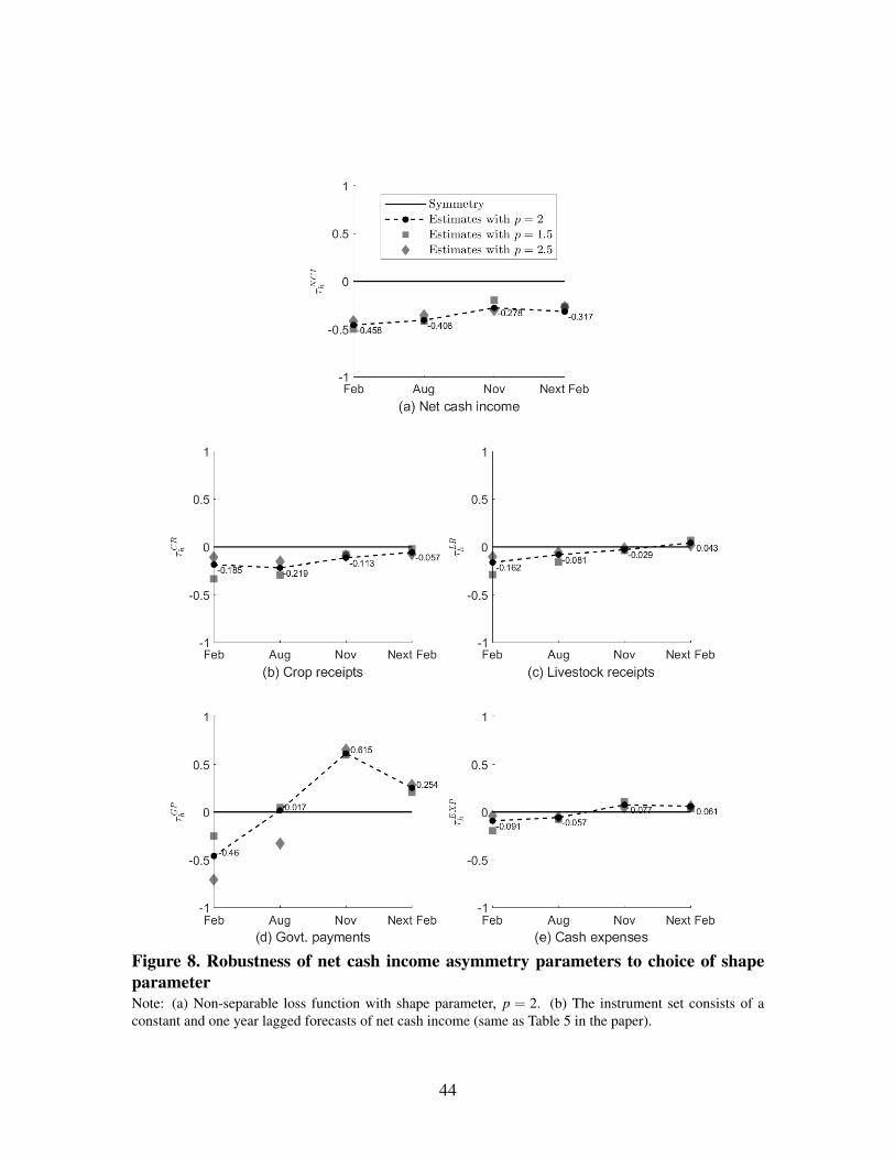
Figure 8. Robustness of net cash income asymmetry parameters to choice of shapeparameterNote: (a) Non-separable loss function with shape parameter, p = 2. (b) The instrument set consists of aconstant and one year lagged forecasts of net cash income (same as Table 5 in the paper).

44

Figure 9. Robustness of net cash income asymmetry parameters to choice of instru-mentsNote: (a) Non-separable loss function with shape parameter, p = 2. (b) The instrument consists of a constantand one year lagged forecasts of 1) net cash income(same as Table 5 in the paper), 2) crop receipts, 3)livestock receipts, 4) government payments, and 5) net cash income and crop receipts.

45

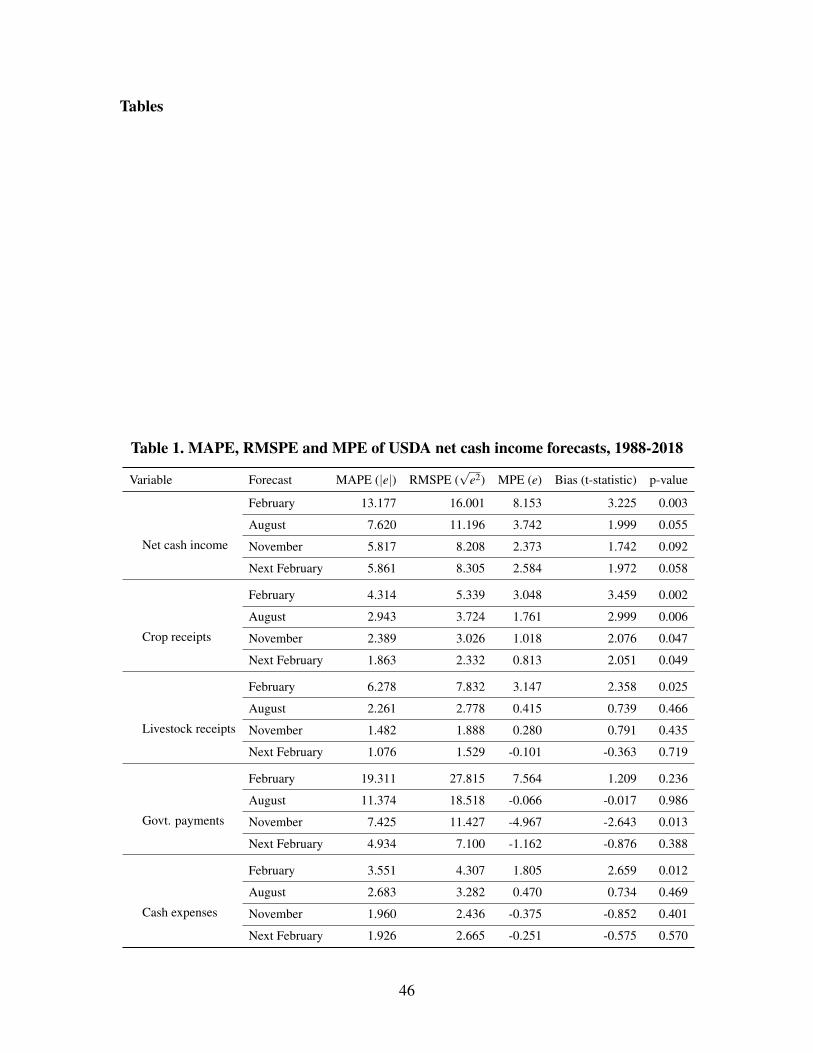
Tables

Table 1. MAPE, RMSPE and MPE of USDA net cash income forecasts, 1988-2018

Variable Forecast MAPE (|e|) RMSPE (√

e2) MPE (e) Bias (t-statistic) p-value

February 13.177 16.001 8.153 3.225 0.003

August 7.620 11.196 3.742 1.999 0.055

November 5.817 8.208 2.373 1.742 0.092Net cash income

Next February 5.861 8.305 2.584 1.972 0.058

February 4.314 5.339 3.048 3.459 0.002

August 2.943 3.724 1.761 2.999 0.006

November 2.389 3.026 1.018 2.076 0.047Crop receipts

Next February 1.863 2.332 0.813 2.051 0.049

February 6.278 7.832 3.147 2.358 0.025

August 2.261 2.778 0.415 0.739 0.466

November 1.482 1.888 0.280 0.791 0.435Livestock receipts

Next February 1.076 1.529 -0.101 -0.363 0.719

February 19.311 27.815 7.564 1.209 0.236

August 11.374 18.518 -0.066 -0.017 0.986

November 7.425 11.427 -4.967 -2.643 0.013Govt. payments

Next February 4.934 7.100 -1.162 -0.876 0.388

February 3.551 4.307 1.805 2.659 0.012

August 2.683 3.282 0.470 0.734 0.469

November 1.960 2.436 -0.375 -0.852 0.401Cash expenses

Next February 1.926 2.665 -0.251 -0.575 0.570

46

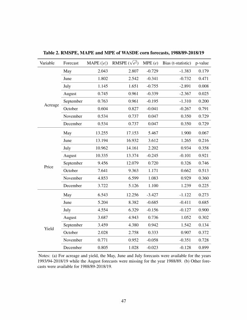
Table 2. RMSPE, MAPE and MPE of WASDE corn forecasts, 1988/89-2018/19

Variable Forecast MAPE (|e|) RMSPE (√

e2) MPE (e) Bias (t-statistic) p-value

May 2.043 2.807 -0.729 -1.383 0.179

June 1.802 2.542 -0.341 -0.732 0.471

July 1.145 1.651 -0.755 -2.891 0.008

August 0.745 0.961 -0.339 -2.367 0.025

September 0.763 0.961 -0.195 -1.310 0.200

October 0.604 0.827 -0.041 -0.267 0.791

November 0.534 0.737 0.047 0.350 0.729

Acreage

December 0.534 0.737 0.047 0.350 0.729

May 13.255 17.153 5.467 1.900 0.067

June 13.194 16.932 3.612 1.265 0.216

July 10.962 14.161 2.202 0.934 0.358

August 10.335 13.374 -0.245 -0.101 0.921

September 9.456 12.079 0.720 0.326 0.746

October 7.641 9.363 1.171 0.662 0.513

November 4.853 6.599 1.083 0.929 0.360

Price

December 3.722 5.126 1.100 1.239 0.225

May 6.543 12.256 -3.427 -1.122 0.273

June 5.204 8.382 -0.685 -0.411 0.685

July 4.554 6.329 -0.156 -0.127 0.900

August 3.687 4.943 0.736 1.052 0.302

September 3.459 4.380 0.942 1.542 0.134

October 2.028 2.758 0.333 0.907 0.372

November 0.771 0.952 -0.058 -0.351 0.728

Yield

December 0.805 1.028 -0.023 -0.128 0.899

Notes: (a) For acreage and yield, the May, June and July forecasts were available for the years1993/94-2018/19 while the August forecasts were missing for the year 1988/89. (b) Other fore-casts were available for 1988/89-2018/19.

47

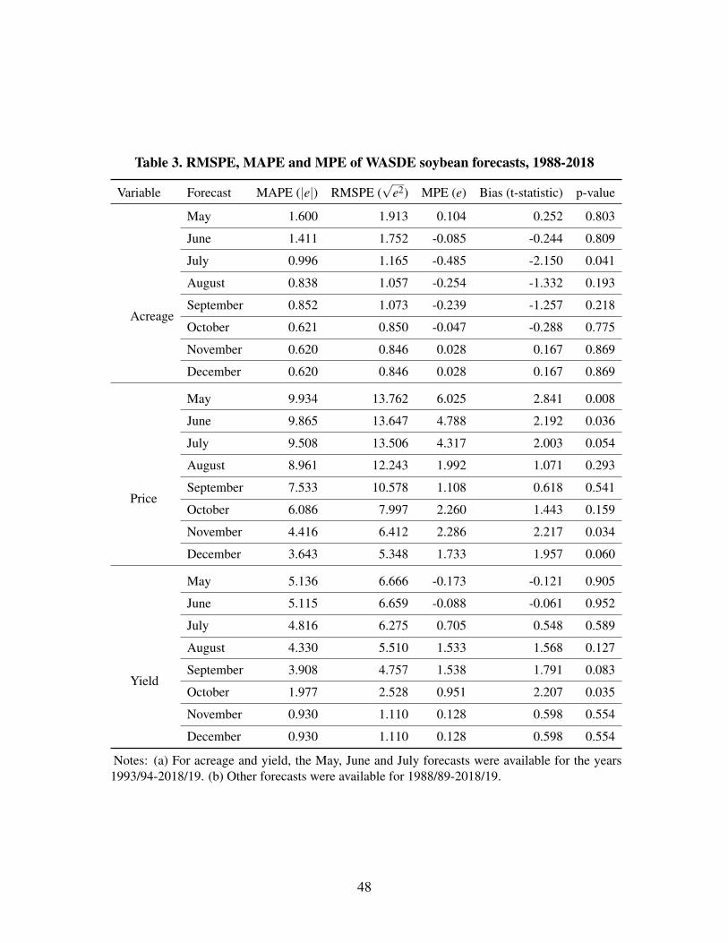
Table 3. RMSPE, MAPE and MPE of WASDE soybean forecasts, 1988-2018

Variable Forecast MAPE (|e|) RMSPE (√

e2) MPE (e) Bias (t-statistic) p-value

May 1.600 1.913 0.104 0.252 0.803

June 1.411 1.752 -0.085 -0.244 0.809

July 0.996 1.165 -0.485 -2.150 0.041

August 0.838 1.057 -0.254 -1.332 0.193

September 0.852 1.073 -0.239 -1.257 0.218

October 0.621 0.850 -0.047 -0.288 0.775

November 0.620 0.846 0.028 0.167 0.869

Acreage

December 0.620 0.846 0.028 0.167 0.869

May 9.934 13.762 6.025 2.841 0.008

June 9.865 13.647 4.788 2.192 0.036

July 9.508 13.506 4.317 2.003 0.054

August 8.961 12.243 1.992 1.071 0.293

September 7.533 10.578 1.108 0.618 0.541

October 6.086 7.997 2.260 1.443 0.159

November 4.416 6.412 2.286 2.217 0.034

Price

December 3.643 5.348 1.733 1.957 0.060

May 5.136 6.666 -0.173 -0.121 0.905

June 5.115 6.659 -0.088 -0.061 0.952

July 4.816 6.275 0.705 0.548 0.589

August 4.330 5.510 1.533 1.568 0.127

September 3.908 4.757 1.538 1.791 0.083

October 1.977 2.528 0.951 2.207 0.035

November 0.930 1.110 0.128 0.598 0.554

Yield

December 0.930 1.110 0.128 0.598 0.554

Notes: (a) For acreage and yield, the May, June and July forecasts were available for the years1993/94-2018/19. (b) Other forecasts were available for 1988/89-2018/19.

48

Table 4. MAPE, RMSPE and MPE of WASDE wheat forecasts, 1988-2018

Variable Forecast MAPE (|e|) RMSPE (√

e2) MPE (e) Bias (t-statistic) p-value

May 2.158 2.700 -0.407 -0.763 0.452

June 2.142 2.663 -0.301 -0.535 0.598

July 1.272 1.625 -1.145 -5.660 0.000

August 1.056 1.351 -0.903 -4.839 0.000Acreage

September 1.056 1.351 -0.903 -4.839 0.000

May 11.840 14.839 2.583 0.935 0.357

June 11.083 13.653 2.220 0.886 0.383

July 8.570 10.794 2.709 1.401 0.172

August 6.435 7.866 1.169 0.797 0.432Price

September 4.812 5.774 1.056 1.004 0.324

May 4.759 5.923 2.149 1.943 0.063

June 3.957 4.749 1.985 2.302 0.030

July 2.470 3.358 0.797 1.591 0.123

August 1.674 2.173 0.259 0.736 0.468Yield

September 1.230 1.607 0.186 0.638 0.528

Notes: (a) For acreage and yield, the May and June forecasts were available for the years 1993/94-2018/19 while the July forecasts were missing for the year 1988/89. (b) Other forecasts wereavailable for 1988/89-2018/19.

49

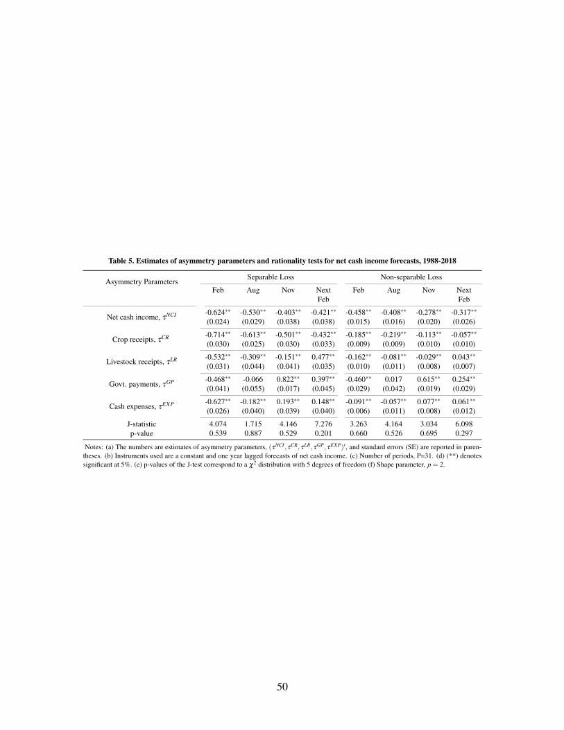
Table 5. Estimates of asymmetry parameters and rationality tests for net cash income forecasts, 1988-2018

Asymmetry ParametersSeparable Loss Non-separable Loss

Feb Aug Nov NextFeb

Feb Aug Nov NextFeb

Net cash income, τNCI -0.624∗∗ -0.530∗∗ -0.403∗∗ -0.421∗∗ -0.458∗∗ -0.408∗∗ -0.278∗∗ -0.317∗∗

(0.024) (0.029) (0.038) (0.038) (0.015) (0.016) (0.020) (0.026)

Crop receipts, τCR -0.714∗∗ -0.613∗∗ -0.501∗∗ -0.432∗∗ -0.185∗∗ -0.219∗∗ -0.113∗∗ -0.057∗∗

(0.030) (0.025) (0.030) (0.033) (0.009) (0.009) (0.010) (0.010)

Livestock receipts, τLR -0.532∗∗ -0.309∗∗ -0.151∗∗ 0.477∗∗ -0.162∗∗ -0.081∗∗ -0.029∗∗ 0.043∗∗

(0.031) (0.044) (0.041) (0.035) (0.010) (0.011) (0.008) (0.007)

Govt. payments, τGP -0.468∗∗ -0.066 0.822∗∗ 0.397∗∗ -0.460∗∗ 0.017 0.615∗∗ 0.254∗∗

(0.041) (0.055) (0.017) (0.045) (0.029) (0.042) (0.019) (0.029)

Cash expenses, τEXP -0.627∗∗ -0.182∗∗ 0.193∗∗ 0.148∗∗ -0.091∗∗ -0.057∗∗ 0.077∗∗ 0.061∗∗

(0.026) (0.040) (0.039) (0.040) (0.006) (0.011) (0.008) (0.012)

J-statistic 4.074 1.715 4.146 7.276 3.263 4.164 3.034 6.098p-value 0.539 0.887 0.529 0.201 0.660 0.526 0.695 0.297

Notes: (a) The numbers are estimates of asymmetry parameters, (τNCI,τCR,τLR,τGP,τEXP)′, and standard errors (SE) are reported in paren-theses. (b) Instruments used are a constant and one year lagged forecasts of net cash income. (c) Number of periods, P=31. (d) (**) denotessignificant at 5%. (e) p-values of the J-test correspond to a χ2 distribution with 5 degrees of freedom (f) Shape parameter, p = 2.

50

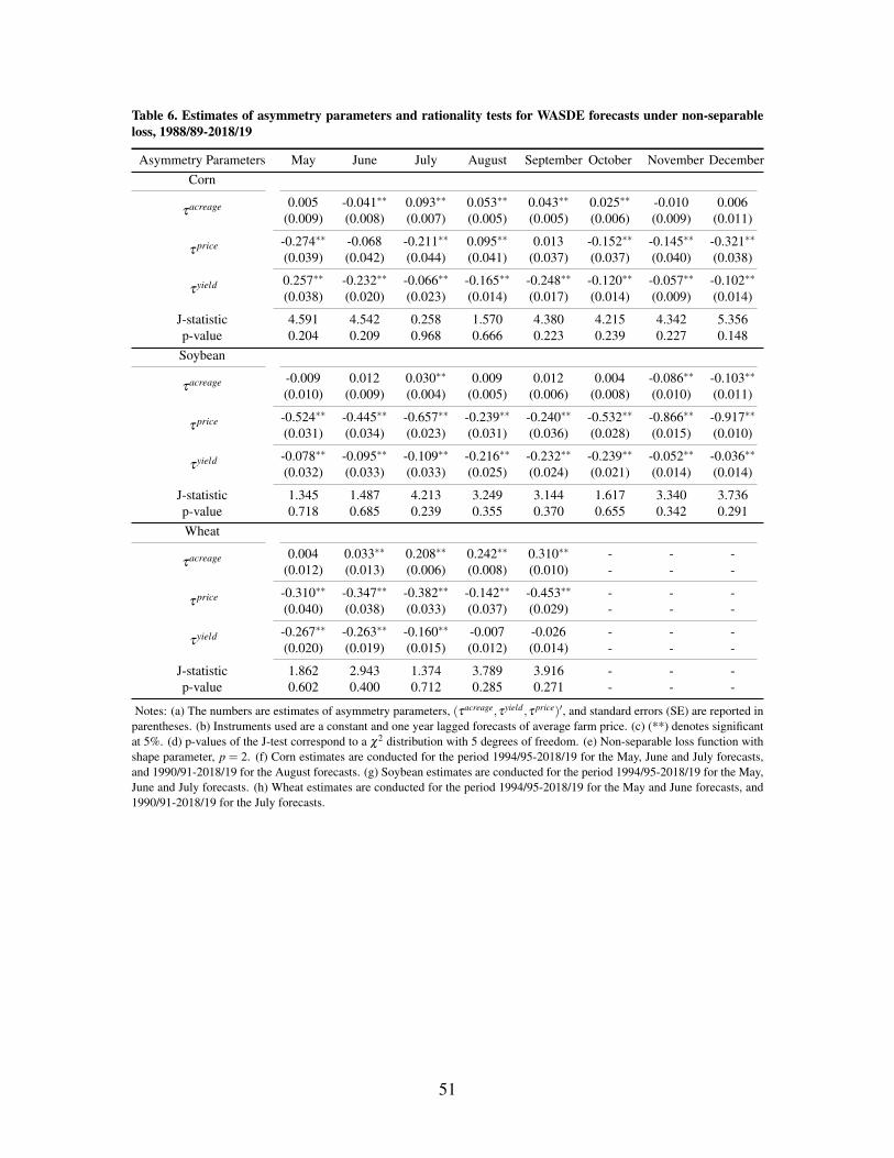
Table 6. Estimates of asymmetry parameters and rationality tests for WASDE forecasts under non-separableloss, 1988/89-2018/19

Asymmetry Parameters May June July August September October November DecemberCorn

τacreage 0.005 -0.041∗∗ 0.093∗∗ 0.053∗∗ 0.043∗∗ 0.025∗∗ -0.010 0.006(0.009) (0.008) (0.007) (0.005) (0.005) (0.006) (0.009) (0.011)

τ price -0.274∗∗ -0.068 -0.211∗∗ 0.095∗∗ 0.013 -0.152∗∗ -0.145∗∗ -0.321∗∗

(0.039) (0.042) (0.044) (0.041) (0.037) (0.037) (0.040) (0.038)

τyield 0.257∗∗ -0.232∗∗ -0.066∗∗ -0.165∗∗ -0.248∗∗ -0.120∗∗ -0.057∗∗ -0.102∗∗

(0.038) (0.020) (0.023) (0.014) (0.017) (0.014) (0.009) (0.014)

J-statistic 4.591 4.542 0.258 1.570 4.380 4.215 4.342 5.356p-value 0.204 0.209 0.968 0.666 0.223 0.239 0.227 0.148Soybean

τacreage -0.009 0.012 0.030∗∗ 0.009 0.012 0.004 -0.086∗∗ -0.103∗∗

(0.010) (0.009) (0.004) (0.005) (0.006) (0.008) (0.010) (0.011)

τ price -0.524∗∗ -0.445∗∗ -0.657∗∗ -0.239∗∗ -0.240∗∗ -0.532∗∗ -0.866∗∗ -0.917∗∗

(0.031) (0.034) (0.023) (0.031) (0.036) (0.028) (0.015) (0.010)

τyield -0.078∗∗ -0.095∗∗ -0.109∗∗ -0.216∗∗ -0.232∗∗ -0.239∗∗ -0.052∗∗ -0.036∗∗

(0.032) (0.033) (0.033) (0.025) (0.024) (0.021) (0.014) (0.014)

J-statistic 1.345 1.487 4.213 3.249 3.144 1.617 3.340 3.736p-value 0.718 0.685 0.239 0.355 0.370 0.655 0.342 0.291Wheat

τacreage 0.004 0.033∗∗ 0.208∗∗ 0.242∗∗ 0.310∗∗ - - -(0.012) (0.013) (0.006) (0.008) (0.010) - - -

τ price -0.310∗∗ -0.347∗∗ -0.382∗∗ -0.142∗∗ -0.453∗∗ - - -(0.040) (0.038) (0.033) (0.037) (0.029) - - -

τyield -0.267∗∗ -0.263∗∗ -0.160∗∗ -0.007 -0.026 - - -(0.020) (0.019) (0.015) (0.012) (0.014) - - -

J-statistic 1.862 2.943 1.374 3.789 3.916 - - -p-value 0.602 0.400 0.712 0.285 0.271 - - -

Notes: (a) The numbers are estimates of asymmetry parameters, (τacreage,τyield ,τ price)′, and standard errors (SE) are reported inparentheses. (b) Instruments used are a constant and one year lagged forecasts of average farm price. (c) (**) denotes significantat 5%. (d) p-values of the J-test correspond to a χ2 distribution with 5 degrees of freedom. (e) Non-separable loss function withshape parameter, p = 2. (f) Corn estimates are conducted for the period 1994/95-2018/19 for the May, June and July forecasts,and 1990/91-2018/19 for the August forecasts. (g) Soybean estimates are conducted for the period 1994/95-2018/19 for the May,June and July forecasts. (h) Wheat estimates are conducted for the period 1994/95-2018/19 for the May and June forecasts, and1990/91-2018/19 for the July forecasts.

51

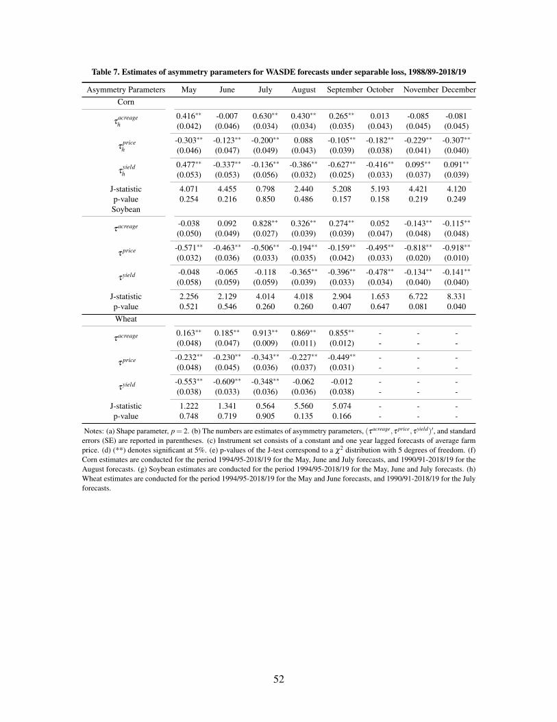
Table 7. Estimates of asymmetry parameters for WASDE forecasts under separable loss, 1988/89-2018/19

Asymmetry Parameters May June July August September October November DecemberCorn

τacreageh

0.416∗∗ -0.007 0.630∗∗ 0.430∗∗ 0.265∗∗ 0.013 -0.085 -0.081(0.042) (0.046) (0.034) (0.034) (0.035) (0.043) (0.045) (0.045)

τpriceh

-0.303∗∗ -0.123∗∗ -0.200∗∗ 0.088 -0.105∗∗ -0.182∗∗ -0.229∗∗ -0.307∗∗

(0.046) (0.047) (0.049) (0.043) (0.039) (0.038) (0.041) (0.040)

τyieldh

0.477∗∗ -0.337∗∗ -0.136∗∗ -0.386∗∗ -0.627∗∗ -0.416∗∗ 0.095∗∗ 0.091∗∗

(0.053) (0.053) (0.056) (0.032) (0.025) (0.033) (0.037) (0.039)

J-statistic 4.071 4.455 0.798 2.440 5.208 5.193 4.421 4.120p-value 0.254 0.216 0.850 0.486 0.157 0.158 0.219 0.249Soybean

τacreage -0.038 0.092 0.828∗∗ 0.326∗∗ 0.274∗∗ 0.052 -0.143∗∗ -0.115∗∗

(0.050) (0.049) (0.027) (0.039) (0.039) (0.047) (0.048) (0.048)

τ price -0.571∗∗ -0.463∗∗ -0.506∗∗ -0.194∗∗ -0.159∗∗ -0.495∗∗ -0.818∗∗ -0.918∗∗

(0.032) (0.036) (0.033) (0.035) (0.042) (0.033) (0.020) (0.010)

τyield -0.048 -0.065 -0.118 -0.365∗∗ -0.396∗∗ -0.478∗∗ -0.134∗∗ -0.141∗∗

(0.058) (0.059) (0.059) (0.039) (0.033) (0.034) (0.040) (0.040)

J-statistic 2.256 2.129 4.014 4.018 2.904 1.653 6.722 8.331p-value 0.521 0.546 0.260 0.260 0.407 0.647 0.081 0.040Wheat

τacreage 0.163∗∗ 0.185∗∗ 0.913∗∗ 0.869∗∗ 0.855∗∗ - - -(0.048) (0.047) (0.009) (0.011) (0.012) - - -

τ price -0.232∗∗ -0.230∗∗ -0.343∗∗ -0.227∗∗ -0.449∗∗ - - -(0.048) (0.045) (0.036) (0.037) (0.031) - - -

τyield -0.553∗∗ -0.609∗∗ -0.348∗∗ -0.062 -0.012 - - -(0.038) (0.033) (0.036) (0.036) (0.038) - - -

J-statistic 1.222 1.341 0.564 5.560 5.074 - - -p-value 0.748 0.719 0.905 0.135 0.166 - - -

Notes: (a) Shape parameter, p= 2. (b) The numbers are estimates of asymmetry parameters, (τacreage,τ price,τyield)′, and standarderrors (SE) are reported in parentheses. (c) Instrument set consists of a constant and one year lagged forecasts of average farmprice. (d) (**) denotes significant at 5%. (e) p-values of the J-test correspond to a χ2 distribution with 5 degrees of freedom. (f)Corn estimates are conducted for the period 1994/95-2018/19 for the May, June and July forecasts, and 1990/91-2018/19 for theAugust forecasts. (g) Soybean estimates are conducted for the period 1994/95-2018/19 for the May, June and July forecasts. (h)Wheat estimates are conducted for the period 1994/95-2018/19 for the May and June forecasts, and 1990/91-2018/19 for the Julyforecasts.

52

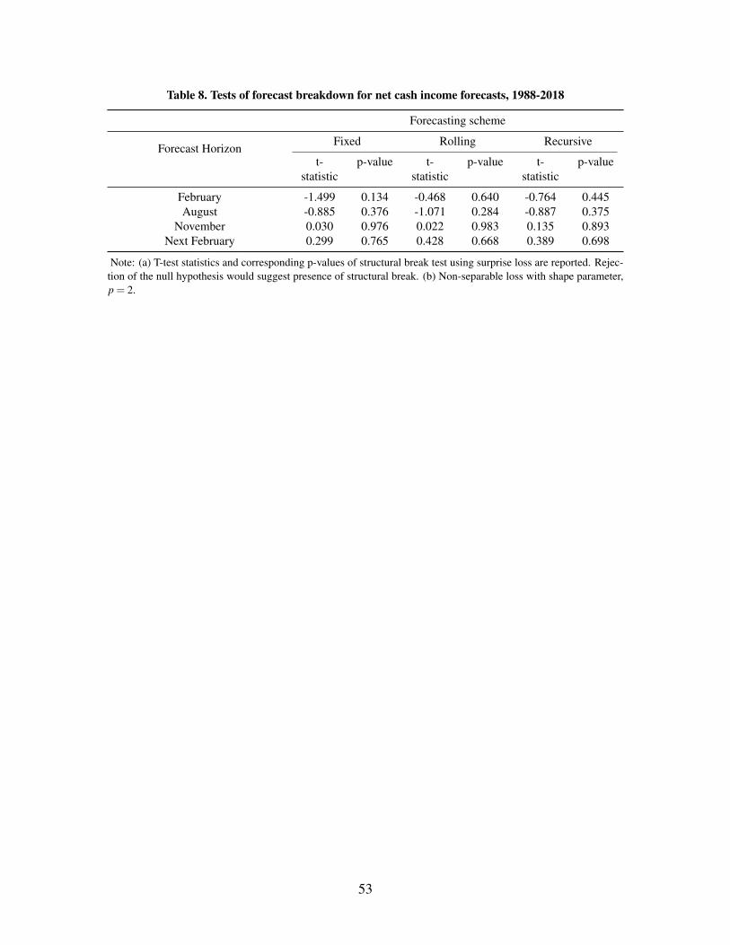
Table 8. Tests of forecast breakdown for net cash income forecasts, 1988-2018

Forecasting scheme

Forecast HorizonFixed Rolling Recursive

t-statistic

p-value t-statistic

p-value t-statistic

p-value

February -1.499 0.134 -0.468 0.640 -0.764 0.445August -0.885 0.376 -1.071 0.284 -0.887 0.375

November 0.030 0.976 0.022 0.983 0.135 0.893Next February 0.299 0.765 0.428 0.668 0.389 0.698

Note: (a) T-test statistics and corresponding p-values of structural break test using surprise loss are reported. Rejec-tion of the null hypothesis would suggest presence of structural break. (b) Non-separable loss with shape parameter,p = 2.

53

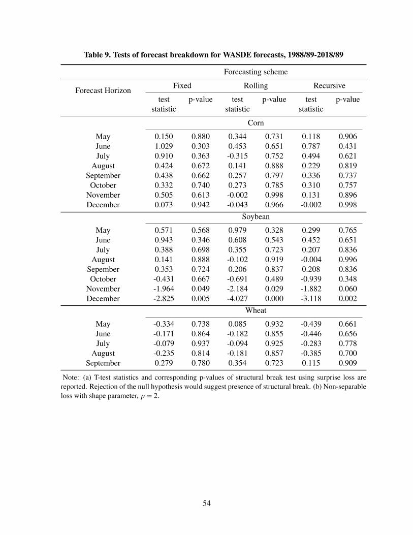
Table 9. Tests of forecast breakdown for WASDE forecasts, 1988/89-2018/89

Forecasting scheme

Forecast HorizonFixed Rolling Recursive

teststatistic

p-value teststatistic

p-value teststatistic

p-value

Corn

May 0.150 0.880 0.344 0.731 0.118 0.906June 1.029 0.303 0.453 0.651 0.787 0.431July 0.910 0.363 -0.315 0.752 0.494 0.621

August 0.424 0.672 0.141 0.888 0.229 0.819September 0.438 0.662 0.257 0.797 0.336 0.737

October 0.332 0.740 0.273 0.785 0.310 0.757November 0.505 0.613 -0.002 0.998 0.131 0.896December 0.073 0.942 -0.043 0.966 -0.002 0.998

Soybean

May 0.571 0.568 0.979 0.328 0.299 0.765June 0.943 0.346 0.608 0.543 0.452 0.651July 0.388 0.698 0.355 0.723 0.207 0.836

August 0.141 0.888 -0.102 0.919 -0.004 0.996Sepember 0.353 0.724 0.206 0.837 0.208 0.836October -0.431 0.667 -0.691 0.489 -0.939 0.348

November -1.964 0.049 -2.184 0.029 -1.882 0.060December -2.825 0.005 -4.027 0.000 -3.118 0.002

Wheat

May -0.334 0.738 0.085 0.932 -0.439 0.661June -0.171 0.864 -0.182 0.855 -0.446 0.656July -0.079 0.937 -0.094 0.925 -0.283 0.778

August -0.235 0.814 -0.181 0.857 -0.385 0.700September 0.279 0.780 0.354 0.723 0.115 0.909

Note: (a) T-test statistics and corresponding p-values of structural break test using surprise loss arereported. Rejection of the null hypothesis would suggest presence of structural break. (b) Non-separableloss with shape parameter, p = 2.

54