The Recoverable Robust Facility Location Problem

Eduardo Alvarez-MirandaDEI, Universita di Bologna, Bologna, Italy; DMGI, Universidad de Talca, Curico, Chile, ealvarez@utalca.cl

Elena FernandezDepartament of Statistics and Operational Research, Universidad Politecnica de Catalunya, Barcelona,

Spain,e.fernandez@upc.edu

Ivana LjubicDepartment of Statistics and Operations Research, Universitat Wien, Vienna, Austria,ivana.ljubic@univie.ac.at

This work deals with a facility location problem in which location and allocation policy is defined in two

stages such that a first-stage solution should be robust against the possible realizations (scenarios) of the

input data that can only be revealed in a second stage. This solution should be robust enough so that

it can be recovered promptly and at low cost in the second stage. In contrast to some related modeling

approaches from the literature, this new recoverable robust model is more general in terms of the considered

data uncertainty; it can address situations in which uncertainty may be present in any of the following four

categories: provider-side uncertainty, receiver-side uncertainty, uncertainty in-between, and uncertainty with

respect to the cost parameters.

For this novel problem, a sophisticated algorithmic framework based on a Benders decomposition approach

is designed and complemented by several non-trivial enhancements, including dual lifting, branching pri-

orities, matheuristics and zero-half cuts. Two large sets of realistic instances that incorporate spatial and

demographic information of countries such as Germany and US (transportation) and Bangladesh and the

Philippines (disaster management) are introduced. They are used to analyze in detail the characteristics of

the proposed model and the obtained solutions as well as the effectiveness, behavior and limitations of the

designed algorithm.

Key words : Facility Location, Two-Stage Robust Optimization, Branch-and-Cut, L-Shaped Cuts

History :

1. Introduction

Nowadays, we are more and more aware of the growing presence of dynamism and uncertainty in

decision making. Fortunately, as the decisions become more complex, the availability of modeling,

algorithmic and computational tools increases as well. Facility location and allocation decisions are

among the most relevant decisions in several private and public logistic contexts and they usually

involve strategic and operative policies with mid and long term impacts. Precisely because of the

practical relevance of these decisions, it is important that they incorporate the uncertainty that

1

2

naturally appears during the planning, modeling and operative process. Such uncertainty can be

represented by different realizations of the input data: customers that actually require a commodity

or a service, locations where the facilities can be located, the network that can be used for con-

necting customers with facilities, and the corresponding costs. The true values of this data usually

become available later in the decision process. In such cases a standard deterministic optimization

model that considers a single possible outcome of the input data can lead towards solutions that

are unlikely to be optimal, or for that matter even feasible, for the final data realization.

Supply chain management is a strategical area in which both uncertainty and facility location

are core elements. For instance, as it is pointed out in (Snyder and Daskin 2005), supply chains

are particularly vulnerable to disruptions (intentional or accidental), imposing the need of taking

into account the possible availability of depots and roads and different structures of the demand.

Likewise, short-term phenomena such as fluctuations in commodity prices (such as oil) or long-term

public policies (such as new toll road concessions) might lead to operational cost increases that

should be considered when deciding the transportation network to be used.

In another context, natural events such as tsunamis, hurricanes or blizzards can produce disas-

trous effects with unpredictable intensity on populated areas and on the transportation infrastruc-

ture. Countries such as Bangladesh and the Philippines are two typical examples; both of them are

regularly hit by hydrological disasters such as floods and typhoons. According to the Department

of Disaster Management of Bangladesh (DDM 2014), every year around 18% of the country is

flooded, which produces over 5000 causalities and the destruction of more than 7 millions of homes.

However, flooded areas my exceed the 75% of the country in case of severe events (as in 1988, 1998

and 2004). In the case of the Philippines, between 6 to 9 typhoons make landfall every year produc-

ing thousands of human losses and incalculable urban destruction; in November of 2013, typhoon

Haiyan produced 6241 causalities and material damage of over 809 millions USD (see PAGASA

2014). In these examples, it is crucial to be able to count with a robust system of humanitarian

relief facilities that even in the worst possible scenario can provide assistance with the quickest

possible response reducing the number of human loses after the occurrence of the event.

The Uncapacitated Facility Location Problem (UFL), also referred as the Simple Plant Location

Problem, is one of the fundamental models in the wide spectrum of Facility Location problems (see,

e.g., recent overviews presented in Eiselt and Marianov 2011, Daskin 2013). In the classical deter-

ministic version of the UFL one is given the set of customers, the set of locations, the facility set-up

costs and the allocation costs. The goal is to define where to open facilities and how to allocate

the customers to them so that the sum of set-up plus allocation costs is minimized.

In practice, it is usually the case that from the moment that the information is gathered until

the moment in which the solution has to be implemented, some of the data might change with

3

respect to the initial setting. As mentioned above, even if some (rough) idea about customers and

locations is known, changes in demographic, socio-economic, or meteorological factors can lead to

changes in the structure of the demand during the planning horizon, and/or the availability of a

given location to host a facility (even if a facility has been already installed). This means that the

solution obtained using a classical method might become infeasible and a new solution might have

to be redefined from scratch. In these cases it would be better to recognize the presence of different

scenarios for the data and find a solution comprised by first- and second-stage decisions.

Two well-known approaches to deal with uncertainty in optimization are Two-stage Stochastic

Optimization (2SSO) and Robust Optimization (RO). In 2SSO (see Birge and Louveaux 2011) the

solutions are built in two stages. In the first stage, a partial collection of decisions is defined which

are later on completed (in the second stage), when the true data is revealed. Hence, the objective is

to minimize the cost of the first-stage decisions plus the expected cost of the recourse (second-stage)

decisions. The quality of the solutions provided by this model strongly depends on the accuracy of

the random representation of the parameter values (such as probability distributions) that allow

to estimate the second-stage expected cost. Nonetheless, sometimes such accuracy is not available

so the use of RO models dealing with deterministic uncertainty arises as a suitable alternative (see

Kouvelis and Yu 1997, Bertsimas and Sim 2004, Ben-Tal et al. 2010). On the one hand these models

do not require assumptions about the distribution of the uncertain input parameters; but on the

other hand, they are usually meant for calculating single-stage decisions that are immune (in a

certain sense) to all possible realizations of the parameter values.

A novel alternative that combines RO and 2SSO is Two-stage Robust Optimization (2SRO); as

in RO, no stochasticity of the parameters is assumed, and as in 2SSO, decisions are taken in two

stages. In this case, the cost of the second-stage decision is computed by looking at the worst-

case realization of the data. Therefore, the goal of 2SRO is to find a robust first-stage solution

that minimizes both the first-stage cost plus the worst-case second-stage cost among all possible

data outcomes. 2SRO is a rather generic classification of models; for references on different 2SRO

settings we refer the reader to (Ben-Tal et al. 2004, Zhao and Zeng 2012).

One of the possibilities in the 2SRO framework is Recoverable Robustness (see Liebchen et al.

2009). Recalling our practical motivation, assume that the facility location and allocation policy

is defined in two stages such that we are required to find a first-stage solution that should be

robust against the possible realizations (scenarios) of the input data in a second stage. This means

that the first-stage solution is expected to perform reasonably well, in terms of feasibility and/or

optimality, for any possible realization of the uncertain parameters. An essential element of this

approach is the possibility of recovering the solution built in the first stage (i.e., to modify the

previously defined location-allocation policy in order to render it feasible and/or cheaper) once

4

the uncertainty is resolved in a second stage. The recovery plan is comprised by recovery actions

which are known in advance and whose costs might also depend on the possible scenario. This

recovery plan is limited, in the sense that the effort needed to recover a solution may be limited

algorithmically (in terms of how a solution may be modified) and economically (in terms of the

total cost of recovery actions). Therefore, instead of looking for a static solution that is robust

against all possible scenarios without allowing any kind of recovery (which is the case for many RO

approaches, see Ben-Tal et al. 2010), we want a solution robust enough so that it can be recovered

promptly and at low cost once the uncertainty is resolved. This balance between robustness and

recoverability is what defines a recoverable robust optimization problem.

With respect to the UFL, we want to find a solution whose first-stage component (opening

of some facilities and allocating some customers) is implemented before the complete realization

of the data. This solution can then be recovered in the second stage (to turn it into a feasible

one) once the actual sets of customers and locations become available. In this case the recovery

actions correspond to the opening of new facilities, the establishment of new allocations and the

re-allocation of customers.

The Recoverable Robust UFL (RRUFL) looks for a solution that minimizes the sum of the first-

stage costs plus the second-stage robust recovery cost defined as the the worst case recovery cost

over all possible scenarios. A formal definition of the RRUFL is given in §2.1.

1.1. Our Contribution and Outline of the Paper

The contributions of this work can be summarized as follows: (i) Due to the nature of the con-

sidered uncertainty, we use a recent concept of recoverable robust optimization to formulate a

Mixed Integer Programming (MIP) model that allows to derive a facility location and alloca-

tion policy composed by first- and second-stage decisions; (ii) for this novel problem we design a

sophisticated algorithmic framework based on Benders decomposition which is complemented by

several non-trivial enhancements; (iii) using instances from two different large classes (representing

transportation and disaster management settings) we analyze in detail the characteristics of the

proposed model and the obtained solutions as well as the effectiveness, behavior, and limitations

of the designed approach.

In §2 the concept of Recoverable Robustness is presented and the RRUFL is formally defined.

The proposed algorithmic framework is described in §3. The description of the benchmark instances

and a detailed analysis of the computational results are presented in §4. Finally, conclusions and

final remarks are given in §5.

5

1.2. The Uncapacitated Facility Location Problem

It is hard to establish a single seminal work presenting the UFL, nonetheless (Kuehn and Hamburger

1963) is usually regarded as the earliest work where the UFL is presented as commonly known

today. We refer the reader to (Cornuejols et al. 1990, Verter 2011) (including the references therein)

for comprehensive surveys on the UFL and some of its variants.

A MIP formulation for the UFL can be given as follows. Let R be the set of customers, J the

set of potential location of facilities, and A a set of links (i, j) connecting customers i in R with

locations j in J (A⊆R× J). The cost of opening a facility at location j ∈ J is given by fj, and

the cost of assigning customer i ∈ R to facility j ∈ J using an existing link (i, j) is given by cij.

Let y ∈ {0,1}|J| be a vector of binary variables such that yj = 1 if a facility is opened at location

j ∈ J and yj = 0 otherwise, and let x∈ {0,1}|A| be a vector of binary variables such that xij = 1 if

customer i∈R is allocated to a facility in j ∈ J using link (i, j)∈A. Using this notation, the UFL

can be formulated as follows:

OPT = min∑j∈J

fjyj +∑

(i,j)∈A

cijxij

s.t.∑

(i,j)∈A

xij = 1, ∀i∈R

xij ≤ yj, ∀(i, j)∈A, ∀j ∈ J

y ∈ {0,1}|J| and x∈ [0,1]|A|.

Despite its simple definition, the UFL is known to be NP-Hard (Cornuejols et al. 1990); however,

the current advances in MIP solvers, computing machinery and the development of sophisticated

preprocessing techniques allow to find optimal or nearly optimal solutions for large instances of the

UFL within reasonable time. We refer to (Letchford and Miller 2012) for recent works on reduction

procedures for the UFL.

The incorporation of different types of uncertainty when modeling and solving the UFL is not

new; in §2.2 we will provide a brief review of Facility Location under uncertainty and compare our

setting with previously proposed problems.

2. The Recoverable Robust UFL

In this section we present a literature review on Recoverable Robustness and formally define the

RRUFL.

Recoverable Robust Optimization Recoverable Robust Optimization (RRO) was first intro-

duced in (Liebchen et al. 2007, 2009) as a tool for decision making under uncertainty in applications

arising in the railway scheduling. In (Cacchiani et al. 2008) and (D’Angelo et al. 2011) one can

find further applications of RRO in the context of railway scheduling.

6

In the last couple of years, RRO has been applied to other problems. The recoverable robust

knapsack problem considering different models of uncertainty is studied in (Busing et al. 2011).

Formulations and algorithms for different variants of the recoverable robust shortest path problem

are given in (Busing 2012). Models, properties and exact algorithms for recoverable robust two-level

network design problems are presented in (Alvarez-Miranda et al. 2013). A more general framework

of the RRO is studied in (Cicerone et al. 2012) where multiple recovery stages are allowed. The

authors apply this new model to timetabling and delay management applications.

Different types of uncertainty, e.g., interval, polyhedral and discrete sets, can be included in the

decision process trough RRO. In this paper, we use discrete sets to model the uncertainty.

2.1. A Formulation of the RRUFL

As mentioned above, facility location along with the corresponding allocation decisions are typically

exposed to uncertainty in different input data. As described in (Shen et al. 2011), it is possible to

classify uncertainty in three categories: provider-side uncertainty, receiver-side uncertainty, and in-

between uncertainty. The first corresponds to the uncertainty in facility capacity, facility reliability,

facility availability, etc.; the second is related to the uncertain structure of the set of customers,

customer demands, customer locations, etc.; and the third refers to the lack of complete knowledge

about the transportation network topology, transportation times or costs between facilities and

customers. The proposed recoverable robust UFL model is a general approach and it can address

situations in which uncertainty may be present in any of these three categories.

Suppose we are given an instance of the UFL in which uncertainty is present in the set of

customers R, the set of locations J , the set of allocation links A and the corresponding set-up and

allocation costs. Such application might arise, for instance, in the event of natural disasters. In

these cases it can be very hard to estimate in advance (i) which areas will require humanitarian

relief, (ii) where the emergency facilities (e.g., Red Cross facilities) can be located and (iii) how

the damaged areas can be reached by the emergency brigades coming from the installed facilities.

Therefore, instead of dealing with deterministic sets R, J and A we are given a finite set K of

discrete scenarios such that each scenario k ∈K is characterized by its own sets Rk, Jk and Ak

and also by the corresponding set-up and allocation costs.

Formally, let K be a set of scenarios representing possible realizations of the problem data, more

precisely, for a given k ∈K: let Rk be the set of customers that require the service if scenario k is

realized; let Jk be the set of locations where facilities can be opened if scenario k is realized; and

let Ak be the set of links that can be used if scenario k is realized. We define R0 =⋃k∈K R

k as the

set of potential customers, J0 =⋃k∈K J

k as the set of potential locations and A0 =⋃k∈K A

k as the

set of potential connections. We assume that the classical UFL has at least one feasible solution

for R0, J0 and A0, and that each customer i∈Rk can be reached by some link from Ak.

7

The decision maker faces a two-stage decision: she/he needs to define a first-stage plan (to open

some facilities and to allocate some customers to these open facilities) without knowing in advance

the actual data that will be revealed. Once the actual information is available in a second stage

(i.e., a single k ∈K and its corresponding Rk, Jk and Ak) additional decisions can be taken in

order to recover the first-stage plan and turn it into a feasible solution for the revealed data. A

second-stage decision is said to be feasible if for all k ∈K each customer i∈Rk is allocated to one

installed facility in j ∈ Jk and the allocation link is operational, i.e., (i, j)∈Ak. These second-stage

decisions consist of (i) the opening of new facilities, (ii) the allocation of customers to facilities that

are either opened in the second-stage or were opened in the first-stage, and (iii) the re-allocation

of customers that were allocated in the first-stage to facilities that are actually not available in the

realized scenario.

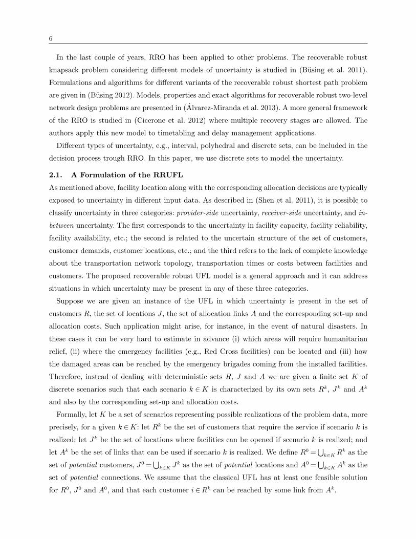
In Figure 1(a) an instance of the RRUFL with set of facilities J0 = {A,B,C}, set of customers

R0 = {1,2,3,4} and with two scenarios is shown. Scenario k = 1 is given by R1 = {1,3,4}, J1 =

{A,B}, A1 = {(1,A), (1, b), (3,A), (4,B)}, and scenario k= 2 is given by R2 = {2,3,4}, J2 = {B,C},A2 = {(2,B), (4,B), (3,C)}. In the first stage, allocation and facility set-up costs are 1 and 2,

respectively. In the second stage, allocation and set-up costs are 1.5 and 3, respectively, the cost

of re-allocating a customer is 2 and the penalty for a facility opened at a non-available site is

3.5. A first-stage solution is shown in Figure 1(b); a facility at site A is opened, customers 1

and 3 are allocated to it and the total cost is: 2 (one opening) + 1 + 1 (two allocations) = 4. For

this given first-stage decision, we present in Figure 1(c) the optimal second-stage solution in case

scenario k = 1 is realized: a facility at site B has to be installed while the facility at A remains

open, customers 1 and 3 keep their allocations while customer 4 is allocated to the facility in

B; so the second-stage cost is: 3 (one opening) + 1.5 (one allocation) = 4.5. The optimal second-

stage solution in case scenario k = 2 is realized is shown in Figure 1(d): facilities at B and C

have to be installed while the facility at A becomes unavailable, customers 2 and 4 are allocated

to the facility at B, while customer 3 has to be re-allocated to the facility in C; the cost is:

3 + 3 (two opening) + 1.5 + 1.5 (two allocations) + 2 (one re-allocation) + 3.5 (one penalty) = 14.5.

Therefore, in the worst case, the overall cost of establishing this first-stage solution and recover it

in the second stage is given as max{4 + 4.5,4 + 14.5}= 18.5. Our goal will be to find the optimal

first-stage decision, so that in the worst-case total cost of the first- and second-stage is minimized.

For this example, the optimal first-stage solution is defined by the installation of a facility in B

and the allocation of 4 to it; this solutions induces a first-stage cost of 3 and worst case second

stage cost of 6, yielding a total cost of 9.

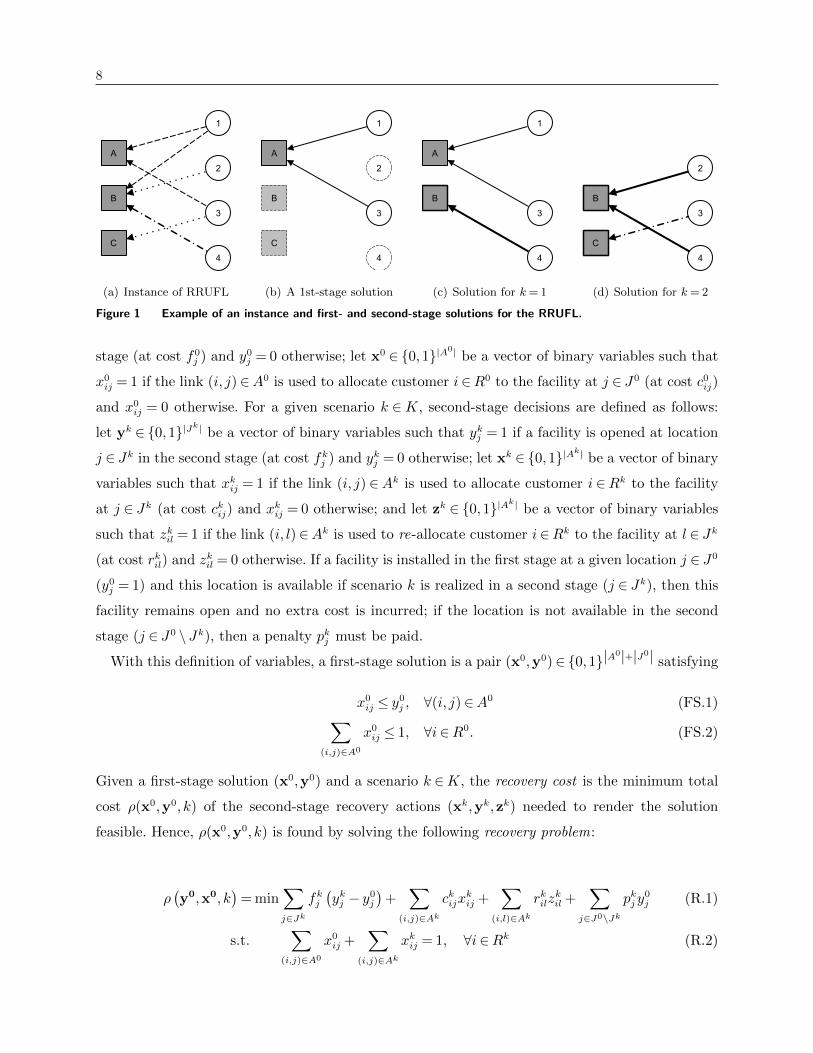
MIP Formulation In the first stage, decisions are modeled as follows: let y0 ∈ {0,1}|J0| be a

vector of binary variables such that y0j = 1 if a facility is opened at location j ∈ J0 in the first

8

(a) Instance of RRUFL (b) A 1st-stage solution (c) Solution for k= 1 (d) Solution for k= 2

Figure 1 Example of an instance and first- and second-stage solutions for the RRUFL.

stage (at cost f0j ) and y0

j = 0 otherwise; let x0 ∈ {0,1}|A0| be a vector of binary variables such that

x0ij = 1 if the link (i, j)∈A0 is used to allocate customer i∈R0 to the facility at j ∈ J0 (at cost c0

ij)

and x0ij = 0 otherwise. For a given scenario k ∈K, second-stage decisions are defined as follows:

let yk ∈ {0,1}|Jk| be a vector of binary variables such that ykj = 1 if a facility is opened at location

j ∈ Jk in the second stage (at cost fkj ) and ykj = 0 otherwise; let xk ∈ {0,1}|Ak| be a vector of binary

variables such that xkij = 1 if the link (i, j) ∈Ak is used to allocate customer i ∈Rk to the facility

at j ∈ Jk (at cost ckij) and xkij = 0 otherwise; and let zk ∈ {0,1}|Ak| be a vector of binary variables

such that zkil = 1 if the link (i, l)∈Ak is used to re-allocate customer i∈Rk to the facility at l ∈ Jk

(at cost rkil) and zkil = 0 otherwise. If a facility is installed in the first stage at a given location j ∈ J0

(y0j = 1) and this location is available if scenario k is realized in a second stage (j ∈ Jk), then this

facility remains open and no extra cost is incurred; if the location is not available in the second

stage (j ∈ J0 \ Jk), then a penalty pkj must be paid.

With this definition of variables, a first-stage solution is a pair (x0,y0)∈ {0,1}|A0|+|J0| satisfying

x0ij ≤ y0

j , ∀(i, j)∈A0 (FS.1)∑(i,j)∈A0

x0ij ≤ 1, ∀i∈R0. (FS.2)

Given a first-stage solution (x0,y0) and a scenario k ∈K, the recovery cost is the minimum total

cost ρ(x0,y0, k) of the second-stage recovery actions (xk,yk,zk) needed to render the solution

feasible. Hence, ρ(x0,y0, k) is found by solving the following recovery problem:

ρ(y0,x0, k

)= min

∑j∈Jk

fkj(ykj − y0

j

)+

∑(i,j)∈Ak

ckijxkij +

∑(i,l)∈Ak

rkilzkil +

∑j∈J0\Jk

pkjy0j (R.1)

s.t.∑

(i,j)∈A0

x0ij +

∑(i,j)∈Ak

xkij = 1, ∀i∈Rk (R.2)

9∑(i,j)∈A0\Ak

x0ij ≤

∑(i,l)∈Ak

zkil, ∀i∈Rk (R.3)

xkij + zkij ≤ ykj , ∀(i, j)∈Ak, ∀i∈Rk (R.4)

y0j ≤ ykj , ∀j ∈ Jk (R.5)

yk ∈ {0,1}|Jk|, xk ∈ {0,1}|A

k|, zk ∈ {0,1}|Ak|. (R.6)

Objective function (R.1) is comprised by the set-up cost of facilities in the second-stage

(∑

j∈Jk fkj (ykj − y0j )), the allocation cost in the second-stage (

∑(i,j)∈Ak ckijx

kij), the cost of re-

allocating customers (∑

(i,l)∈Ak rkilzkil), and the total penalty paid by those facilities opened in the

first stage that can not operate if scenario k ∈ K is realized (∑

j∈J0\Jk pkjy0j ). Constraints (R.2)

state that a customer is either allocated in the first stage (∑

(i,j)∈A0 x0ij) or in the second-stage

(∑

(i,j)∈Ak xkij). Constraints (R.3) model the fact that if a customer i ∈ Rk has been allocated in

the first-stage to a facility j ∈ J0 by means of a link (i, j) ∈A0\Ak then it has to be re-allocated

to another facility l ∈ Jk through a link (i, l) available in the second-stage (∑

(i,l)∈Ak zkil). Con-

straints (R.4) impose that if a customer is allocated or re-allocated to a facility j ∈ Jk, then that

facility has to be available and reachable in the second-stage. The fact that a facility that has been

opened in the first stage should remain opened in the second stage is modeled by (R.5). The nature

of the variables is imposed in (R.6) (note that one can also relax the integrality constraints for xk

and zk, ∀k ∈K).

For a given first-stage solution (x0,y0) the robust recovery cost R(x0,y0) corresponds to the

maximum recovery cost among all k ∈K, i.e.,

R(x0,y0

)= max

k∈Kρ(x0,y0, k

). (RR)

Combining (FS.1)-(FS.2), (R.1)-(R.6) and (RR), we define the Recoverable Robust UFL problem

(RRUFL) as

OPTRR = min∑j∈J0

f0j y

0j +

∑(i,j)∈A0

c0ijx

0ij +R

(x0,y0

)(1)

s.t. (FS.1)-(FS.2), (R.2)-(R.6) and (x0,y0)∈ {0,1}|A0|+|J0|. (2)

In the proposed formulation of the RRUFL we impose that each customer i ∈ Rk has to be

assigned (or re-assigned) to exactly one available facility j ∈ Jk for any given k ∈K. It is possible

to relax this and, instead, impose a penalty, say tki , if customer i∈Rk is not served by any facility

if scenario k is realized. This can be done by introducing a dummy facility πk with a set-up cost

equal to 0 and connecting it to every customer i ∈Rk with an allocation (and re-allocation) cost

ckiπ = rkiπ = tki .

10

In many applications it is natural to think that whichever decision we take in the future it will

be more expensive than if it would have been taken at present. For instance, opening a facility

at a given location is likely to be more expensive later on in the planning horizon than now

(fkj ≥ f0j ). Likewise, an agreement between a depot (facility) and a customer is expected to have

better conditions (for one of the two parties at least) if it is established earlier than if it is defined

when the market conditions have evolved (ckij ≥ c0ij). Furthermore, it is also natural to think that if

an already agreed pact between a depot and a customer is forced to be changed (e.g., because no

allocation link is available between them), this will entail an additional re-allocation cost possibly

higher than the original one (rkil ≥ c0ij, for all l ∈ Jk).

An optimal first-stage solution (x0,y0) is robust because, regardless which scenario occurs, it

guarantees that the second-stage actions will be efficient (due to the minimization of the worst

case) and easy to implement (because only a simple UFL has to be solved). Hence, the more

scenarios we take into consideration to find (x0,y0), the more robust the solution is; because we

are foreseeing more possible states of the future uncertainty. Unlike common approaches of RO

that protect solutions against perturbations in parameters as costs or demands, our approach also

hedges against uncertainty in the very topology of the network. Likewise, a first-stage solution is

recoverable, or possesses recoverability, because it can become feasible in a second stage by means

of second-stage actions.

The Robust UFL without Recovery To assess the effectiveness and benefits of the RRULF,

we also introduce another natural, but more conservative, model. Assume a decision-making context

equivalent to the one taken into account before. Consider a model in which first-stage decisions

are comprised only by y0 and second-stage decisions only by xk, ∀k ∈K. This is, an 2SRO model

in which facilities can be opened only in the first stage and allocations can be decided only in the

second stage. We will refer to this new problem simply as Robust Uncapacitated Facility Location

without Recovery (RUFL). This alternative model lacks the concept of recoverability since the

solution cannot be intrinsically changed: no new facility can be opened and there is no need to

re-allocate any customer in the second stage. Therefore, the solutions of such model although

possibly more robust (since they are more conservative) are expected to be more expensive, either

because unnecessarily many facilities have to be opened in the first stage or because the second-

stage allocation costs are considerably higher than those of the first stage. If we consider again the

instance in Figure 1(a), one can easily see that for this new model the optimal (and only feasible)

first-stage solution would be given by the installation of facilities in A, B and C (with a cost of 6).

In both k= 1 and k= 2 the optimal second-stage cost would be 8. This leads to a total cost equal

to 6 + max{8,8}= 14, which is more than the cost of the optimal solution of the RRUFL which is

9.

11

2.2. The RRUFL and Previously Proposed Problems

Already in the 70’s efforts were devoted to provide both theoretical and algorithmic contributions

on Stochastic UFL. In (Snyder 2006) one can find an excellent review on Facility Location under

uncertainty, describing contributions not only from the stochastic but also from the RO perspective.

More recent references to Facility Location under uncertainty include (Snyder and Daskin 2005,

Averbakh 2005, Snyder and Daskin 2006, Cui et al. 2010, Shen et al. 2011, Albareda-Sambola et al.

2011, Adjiashvili 2012, Gao 2012, Alumur et al. 2012, Albareda-Sambola et al. 2013, Gılpinar et al.

2013) and (Li et al. 2013).

Our definition of the RRUFL, as well as the algorithmic framework described later, spans different

possible cases of uncertainty in Facility Location. Some of them have been already addressed in

the literature by the use of stochastic and robust two-stage models.

For instance if Jk = J0 and Ak = A0, ∀k ∈K, then we are only addressing uncertainty in the

set of customers and, eventually, in the second-stage costs. A 2SSO approach for this problem has

been considered in (Ravi and Sinha 2006), where approximation algorithms have been proposed.

In (Snyder and Daskin 2005, Cui et al. 2010, Shen et al. 2011) and (Li et al. 2013), uncertainty

has been addressed only in the set of locations (Rk = R0 and Ak = A0, ∀k ∈K). As stressed by

the authors, this model is suitable for applications where facilities might become unavailable in a

second stage due to disruptions caused by natural disasters, terrorists attacks or labor strikes (see

Cui et al. 2010). These papers share two important features. First, uncertainty is tackled by means

of 2SSO since probabilities of facility failure are known in advance for each scenario. Second, a

user is assigned to a so-called primary facility that will serve it under normal circumstances, as

well as to a set of ordered backup facilities such that the first of them that is available will serve

the customer when the primary is not available (see Snyder and Daskin 2005). This second feature

cannot be included in our framework without introducing additional binary variables; nonetheless

decision-maker preferences about the re-allocation of a customer in case the originally assigned

facility fails can be incorporated by a proper definition of the re-allocation second-stage costs.

A third case is the one where only connections are subject to uncertainty (Rk =R0 and Jk = J0,

∀k ∈K). A 2SRO model of this case is studied in (Hassin et al. 2009) where the relevance of such

a model of uncertainty is emphasized in the context of response planning after disasters.

3. Algorithmic Framework

Note that formulation (1)-(2) has a polinomial number of variables and constraints with respect to

|R0|, |A0| and |K|. Therefore it can be solved directly (as a compact model) through any state-of-

the-art MIP solver (e.g., CPLEX). However, as we will show later, when large realistic instances

have to be solved, the direct use of solvers turns out to be impractical.

12

Model (1)-(2) is a natural candidate to be solved by means of a Benders-like decomposition

approach: the first-stage variables (x0,y0) are incorporated in the master problem (MP) and the

second-stage variables (xk,yk,zk) are projected out and replaced by a single variable ω representing

the robust recovery cost, for a given (x0, y0), that is computed by solving |K| slave problems

(SPs). Thus, the objective function (1) becomes OPTRR = min∑

j∈J0 f0j y

0j +

∑(i,j)∈A0 c0

ijx0ij + ω,

where ω ≥ ρ (x0,y0, k) ,∀k ∈K. Hence, for each given value of (x0,y0, k), ω can be computed by

independently solving |K| problems (R.1)-(R.6).

One of the main drawbacks of traditional implementations of Benders decomposition for two-

stage integer problems is the need for solving several MIP problems (MP and SPs) at each iteration

in order to obtain a single Benders-cut. Nonetheless, nowadays most of MIP optimization suites

provide branch-and-cut frameworks supported by the use of callbacks. Therefore, a Benders decom-

position algorithm can be transformed into a pure branch-and-cut approach by the use of callbacks.

Benders cuts are added to the model as valid lower-bounds on ω each time a potential solution of

the MP is found by means of solving a Linear Programming (LP) problem in a given node of the

enumeration tree. This technique exploits the benefits of the decomposition allowing to implement

additional methods for heuristically finding more cuts and/or for strengthening the obtained ones.

That way, both, the speed and the convergence of the algorithm can be improved (see Ljubic et al.

2013, Perez-Galarce et al. 2014).

Basic Separation of L-shaped and Integer L-shaped Cuts In our approach, a valid lower

bound on ω is iteratively imposed by means of L-shaped and integer L-shaped cuts (see Van Slyke

and Wets 1967, Laporte and Louveaux 1993). For a given first-stage solution, the second-stage

problem can be decomposed into |K| independent problems: dual variables of the LP-relaxations

of these SPs yield L-shaped cuts that are added to the MP while integer solutions of the SPs yield

integer L-shaped cuts.

At a given node of the enumeration tree, let (x0, y0) be a first-stage solution satisfying (FS.1)-

(FS.2) and let ω be the current value of variable ω. For a given k ∈K, the dual of (R.1)-(R.6) after

removing the integrality constrains can be formulated as

max∑i∈Rk

αi1−

∑(i,j)∈A0

x0ij

+ γi

∑(i,j)∈A0\Ak

x0ij

+∑j∈Jk

(εj − fkj

)y0j +

∑j∈J0\Jk

pkj y0j (D.1)

s.t. αi− δij ≤ ckij, ∀(i, j)∈Ak, ∀i∈Rk (D.2)

γi− δil ≤ rkil, ∀(i, l)∈Ak, ∀i∈Rk (D.3)

εj +∑

(i,j)∈Ak

δij ≤ fkj , ∀j ∈ Jk (D.4)

(α, γ, δ, ε)≥ 0, (D.5)

13

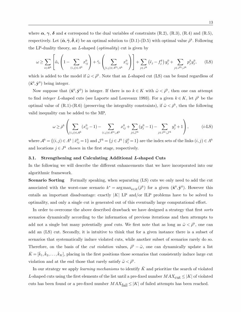
where α, γ, δ and ε correspond to the dual variables of constraints (R.2), (R.3), (R.4) and (R.5),

respectively. Let (α, γ, δ, ε) be an optimal solution to (D.1)-(D.5) with optimal value ρk. Following

the LP-duality theory, an L-shaped (optimality) cut is given by

ω≥∑i∈Rk

αi1−

∑(i,j)∈A0

x0ij

+ γi

∑(i,j)∈A0\Ak

x0ij

+∑j∈Jk

(εj − fkj

)y0j +

∑j∈J0\Jk

pkjy0j , (LS)

which is added to the model if ω < ρk. Note that an L-shaped cut (LS) can be found regardless of

(x0, y0) being integer.

Now suppose that (x0, y0) is integer. If there is no k ∈K with ω < ρk, then one can attempt

to find integer L-shaped cuts (see Laporte and Louveaux 1993). For a given k ∈K, let ρk be the

optimal value of (R.1)-(R.6) (preserving the integrality constraints), if ω < ρk, then the following

valid inequality can be added to the MP,

ω≥ ρk ∑

(i,j)∈Ak

(x0ij − 1)−

∑(i,j)∈Ak\Ak

x0ij +

∑j∈J k

(y0j − 1)−

∑j∈Jk\J k

y0j + 1

, (i-LS)

where Ak = {(i, j)∈Ak | x0ij = 1} and J k = {j ∈ Jk | y0

j = 1} are the index sets of the links (i, j)∈Ak

and locations j ∈ Jk chosen in the first stage, respectively.

3.1. Strengthening and Calculating Additional L-shaped Cuts

In the following we will describe the different enhancements that we have incorporated into our

algorithmic framework.

Scenario Sorting Formally speaking, when separating (LS) cuts we only need to add the cut

associated with the worst-case scenario k∗ = arg maxk∈K(ρk) for a given (x0, y0). However this

entails an important disadvantage: exactly |K| LP and/or ILP problems have to be solved to

optimality, and only a single cut is generated out of this eventually large computational effort.

In order to overcome the above described drawback we have designed a strategy that first sorts

scenarios dynamically according to the information of previous iterations and then attempts to

add not a single but many potentially good cuts. We first note that as long as ω < ρk, one can

add an (LS) cut. Secondly, it is intuitive to think that for a given instance there is a subset of

scenarios that systematically induce violated cuts, while another subset of scenarios rarely do so.

Therefore, on the basis of the cut violation values, ρk − ω, one can dynamically update a list

K = [k1, k2, . . . , kK ], placing in the first positions those scenarios that consistently induce large cut

violation and at the end those that rarely satisfy ω < ρk.

In our strategy we apply learning mechanisms to identify K and prioritize the search of violated

L-shaped cuts using the first elements of the list until a pre-fixed number MAXcut ≤ |K| of violated

cuts has been found or a pre-fixed number MAXfail ≤ |K| of failed attempts has been reached.

14

Algorithm 1 Basic L-shaped cut Separation with Scenario sorting

Input: Fractional solution (x0, y0, ω); vectors freq and viol; MAXcut and MAXfail.

1: K = sortScenarios(K,viol, freq);

2: Set ccut = 0 and cfail = 0;

3: repeat

4: k= getFirst(K);

5: Solve the LP-relaxation of the k−th SP (R.1)-(R.6) and let ρk be the corresponding optimal value;

6: freq[k] = freq[k] + 1 and viol[k] = viol[k] + (ρk − ω);

7: if ω < ρk then

8: Insert an L-shaped cut given by (LS) into the LP;

9: ccut++;

10: else

11: cfail++;

12: until ccut =MAXcut or cfail =MAXfail

13: Resolve the LP;

In Algorithm 1 we present the general scheme of the separation of L-shaped cuts using the

scenario sorting strategy. For each scenario k ∈K, the value freq[k] accumulates the number of

separation calls in which we have solved the corresponding SP. Likewise, the value viol[k] is a

cumulative cut violation value of scenario k, over all previous separation calls. In Step 1 the list

K is created and its elements are sorted in decreasing order with respect to viol[k]/freq[k], which

represents the average violation that each scenario has induced in the previous iterations. In loop 3-

12 the L-shaped cuts are added: in line 4 the first scenario in the list K is taken and removed;

the k−th SP is solved in line 5; both vectors needed to sort scenarios are updated in line 6; if

the solution of the SP induces a violated cut (line 7) then the corresponding inequality is added

in line 8 and the counter of added cuts is increased (line 9); if no violated cut is generated, the

corresponding counter is increased in line 11.

In our default implementation (and after parameter tuning), we have set MAXcut = 0.25× |K|and MAXfail = 0.25× |K|.Dual Lifting Clearly, the strength of the generated L-shaped cuts will strongly influence the

performance of the algorithm; the stronger they are, the less MP iterations (hence, the less explored

nodes in the enumeration tree) are needed. In this paper we use a recently proposed technique to

strengthen L-shaped cuts (see Ljubic et al. 2013). In contrast to other approaches for generating

stronger cuts (see, e.g., Magnanti and Wong 1981), this method does not require to solve any

additional LP problem and the strengthening process can be performed in linear time (with respect

to the number of variables).

Let (x0, y0) be a pair satisfying (FS.1)-(FS.2), ω the current value of variable ω, and (α, γ, δ, ε) an

optimal solution to (D.1)-(D.5) that satisfies ω < ρk. The scheme to strengthen the corresponding

15

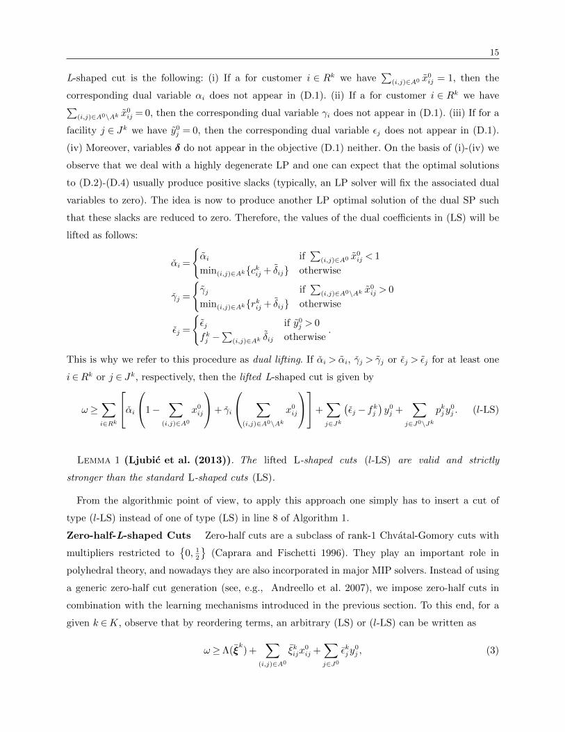
L-shaped cut is the following: (i) If a for customer i ∈ Rk we have∑

(i,j)∈A0 x0ij = 1, then the

corresponding dual variable αi does not appear in (D.1). (ii) If a for customer i ∈ Rk we have∑(i,j)∈A0\Ak x0

ij = 0, then the corresponding dual variable γi does not appear in (D.1). (iii) If for a

facility j ∈ Jk we have y0j = 0, then the corresponding dual variable εj does not appear in (D.1).

(iv) Moreover, variables δ do not appear in the objective (D.1) neither. On the basis of (i)-(iv) we

observe that we deal with a highly degenerate LP and one can expect that the optimal solutions

to (D.2)-(D.4) usually produce positive slacks (typically, an LP solver will fix the associated dual

variables to zero). The idea is now to produce another LP optimal solution of the dual SP such

that these slacks are reduced to zero. Therefore, the values of the dual coefficients in (LS) will be

lifted as follows:

αi =

{αi if

∑(i,j)∈A0 x0

ij < 1

min(i,j)∈Ak{ckij + δij} otherwise

γj =

{γj if

∑(i,j)∈A0\Ak x0

ij > 0

min(i,j)∈Ak{rkij + δij} otherwise

εj =

{εj if y0

j > 0

fkj −∑

(i,j)∈Ak δij otherwise.

This is why we refer to this procedure as dual lifting. If αi > αi, γj > γj or εj > εj for at least one

i∈Rk or j ∈ Jk, respectively, then the lifted L-shaped cut is given by

ω≥∑i∈Rk

αi1−

∑(i,j)∈A0

x0ij

+ γi

∑(i,j)∈A0\Ak

x0ij

+∑j∈Jk

(εj − fkj

)y0j +

∑j∈J0\Jk

pkjy0j . (l-LS)

Lemma 1 (Ljubic et al. (2013)). The lifted L-shaped cuts (l-LS) are valid and strictly

stronger than the standard L-shaped cuts (LS).

From the algorithmic point of view, to apply this approach one simply has to insert a cut of

type (l-LS) instead of one of type (LS) in line 8 of Algorithm 1.

Zero-half-L-shaped Cuts Zero-half cuts are a subclass of rank-1 Chvatal-Gomory cuts with

multipliers restricted to{

0, 12

}(Caprara and Fischetti 1996). They play an important role in

polyhedral theory, and nowadays they are also incorporated in major MIP solvers. Instead of using

a generic zero-half cut generation (see, e.g., Andreello et al. 2007), we impose zero-half cuts in

combination with the learning mechanisms introduced in the previous section. To this end, for a

given k ∈K, observe that by reordering terms, an arbitrary (LS) or (l-LS) can be written as

ω≥Λ(ξk) +

∑(i,j)∈A0

ξkijx0ij +

∑j∈J0

εkjy0j , (3)

16

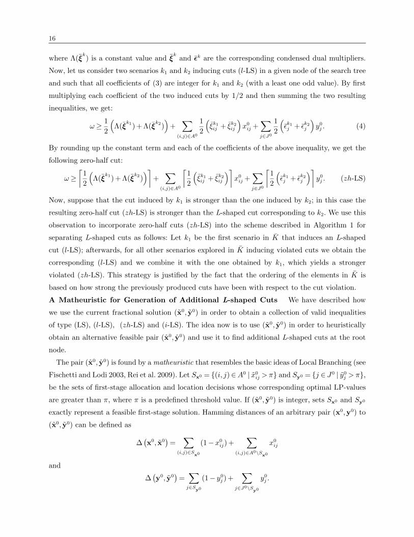
where Λ(ξk) is a constant value and ξ

kand εk are the corresponding condensed dual multipliers.

Now, let us consider two scenarios k1 and k2 inducing cuts (l-LS) in a given node of the search tree

and such that all coefficients of (3) are integer for k1 and k2 (with a least one odd value). By first

multiplying each coefficient of the two induced cuts by 1/2 and then summing the two resulting

inequalities, we get:

ω≥ 1

2

(Λ(ξ

k1) + Λ(ξk2))

+∑

(i,j)∈A0

1

2

(ξk1ij + ξk2

ij

)x0ij +

∑j∈J0

1

2

(εk1j + εk2

j

)y0j . (4)

By rounding up the constant term and each of the coefficients of the above inequality, we get the

following zero-half cut:

ω≥⌈

1

2

(Λ(ξ

k1) + Λ(ξk2))⌉

+∑

(i,j)∈A0

⌈1

2

(ξk1ij + ξk2

ij

)⌉x0ij +

∑j∈J0

⌈1

2

(εk1j + εk2

j

)⌉y0j . (zh-LS)

Now, suppose that the cut induced by k1 is stronger than the one induced by k2; in this case the

resulting zero-half cut (zh-LS) is stronger than the L-shaped cut corresponding to k2. We use this

observation to incorporate zero-half cuts (zh-LS) into the scheme described in Algorithm 1 for

separating L-shaped cuts as follows: Let k1 be the first scenario in K that induces an L-shaped

cut (l-LS); afterwards, for all other scenarios explored in K inducing violated cuts we obtain the

corresponding (l-LS) and we combine it with the one obtained by k1, which yields a stronger

violated (zh-LS). This strategy is justified by the fact that the ordering of the elements in K is

based on how strong the previously produced cuts have been with respect to the cut violation.

A Matheuristic for Generation of Additional L-shaped Cuts We have described how

we use the current fractional solution (x0, y0) in order to obtain a collection of valid inequalities

of type (LS), (l-LS), (zh-LS) and (i-LS). The idea now is to use (x0, y0) in order to heuristically

obtain an alternative feasible pair (x0, y0) and use it to find additional L-shaped cuts at the root

node.

The pair (x0, y0) is found by a matheuristic that resembles the basic ideas of Local Branching (see

Fischetti and Lodi 2003, Rei et al. 2009). Let Sx0 = {(i, j)∈A0 | x0ij >π} and Sy0 = {j ∈ J0 | y0

j >π},be the sets of first-stage allocation and location decisions whose corresponding optimal LP-values

are greater than π, where π is a predefined threshold value. If (x0, y0) is integer, sets Sx0 and Sy0

exactly represent a feasible first-stage solution. Hamming distances of an arbitrary pair (x0,y0) to

(x0, y0) can be defined as

∆(x0, x0

)=

∑(i,j)∈S

x0

(1−x0ij) +

∑(i,j)∈A0\S

x0

x0ij

and

∆(y0, y0

)=∑j∈S

y0

(1− y0j ) +

∑j∈J0\S

y0

y0j .

17

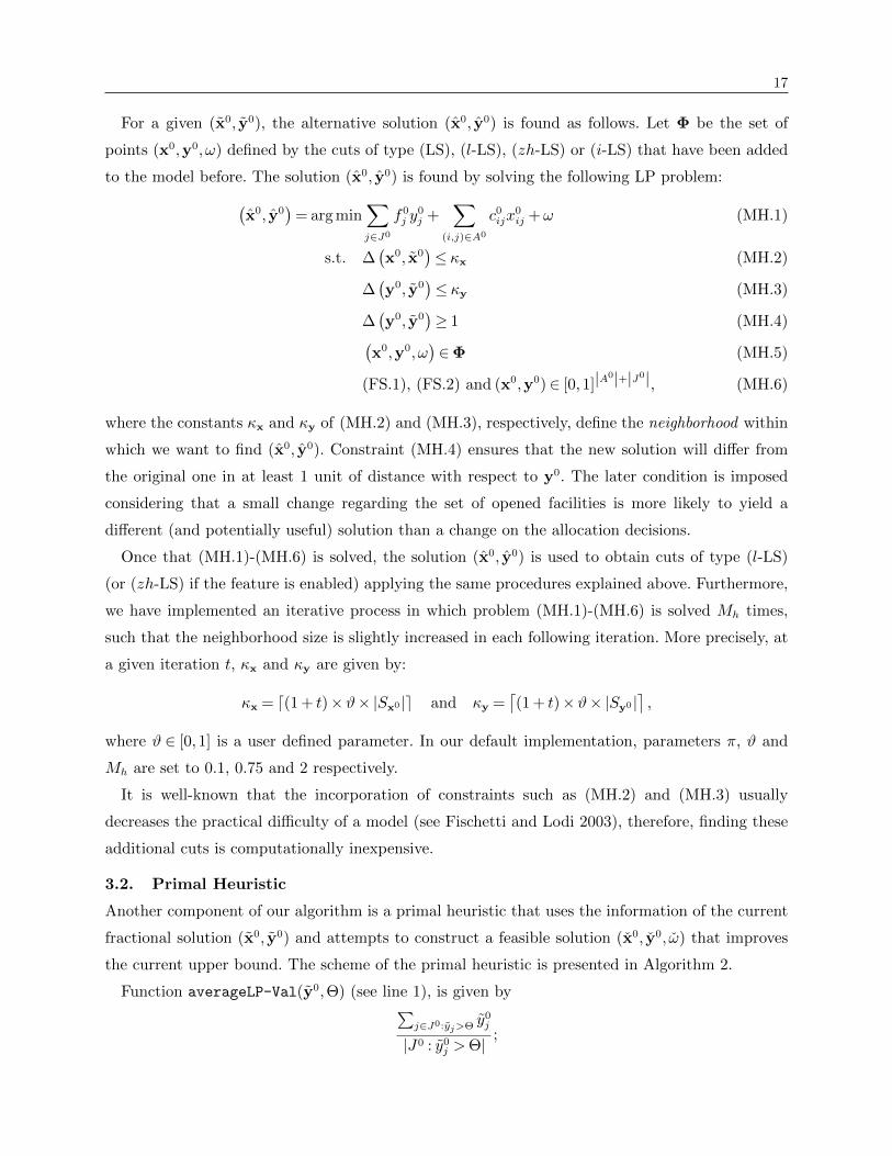
For a given (x0, y0), the alternative solution (x0, y0) is found as follows. Let Φ be the set of

points (x0,y0, ω) defined by the cuts of type (LS), (l-LS), (zh-LS) or (i-LS) that have been added

to the model before. The solution (x0, y0) is found by solving the following LP problem:(x0, y0

)= arg min

∑j∈J0

f0j y

0j +

∑(i,j)∈A0

c0ijx

0ij +ω (MH.1)

s.t. ∆(x0, x0

)≤ κx (MH.2)

∆(y0, y0

)≤ κy (MH.3)

∆(y0, y0

)≥ 1 (MH.4)(

x0,y0, ω)∈Φ (MH.5)

(FS.1), (FS.2) and (x0,y0)∈ [0,1]|A0|+|J0|, (MH.6)

where the constants κx and κy of (MH.2) and (MH.3), respectively, define the neighborhood within

which we want to find (x0, y0). Constraint (MH.4) ensures that the new solution will differ from

the original one in at least 1 unit of distance with respect to y0. The later condition is imposed

considering that a small change regarding the set of opened facilities is more likely to yield a

different (and potentially useful) solution than a change on the allocation decisions.

Once that (MH.1)-(MH.6) is solved, the solution (x0, y0) is used to obtain cuts of type (l-LS)

(or (zh-LS) if the feature is enabled) applying the same procedures explained above. Furthermore,

we have implemented an iterative process in which problem (MH.1)-(MH.6) is solved Mh times,

such that the neighborhood size is slightly increased in each following iteration. More precisely, at

a given iteration t, κx and κy are given by:

κx = d(1 + t)×ϑ× |Sx0 |e and κy =⌈(1 + t)×ϑ× |Sy0 |

⌉,

where ϑ ∈ [0,1] is a user defined parameter. In our default implementation, parameters π, ϑ and

Mh are set to 0.1, 0.75 and 2 respectively.

It is well-known that the incorporation of constraints such as (MH.2) and (MH.3) usually

decreases the practical difficulty of a model (see Fischetti and Lodi 2003), therefore, finding these

additional cuts is computationally inexpensive.

3.2. Primal Heuristic

Another component of our algorithm is a primal heuristic that uses the information of the current

fractional solution (x0, y0) and attempts to construct a feasible solution (x0, y0, ω) that improves

the current upper bound. The scheme of the primal heuristic is presented in Algorithm 2.

Function averageLP-Val(y0,Θ) (see line 1), is given by∑j∈J0:yj>Θ y

0j

|J0 : y0j >Θ|

;

18

Algorithm 2 Primal Heuristic

Input: Fractional solution (x0, y0, ω); threshold Θ.

1: y= averageLP-Val(y0,Θ);

2: x= averageLP-Val(x0,Θ);

3: Initialize J0 = ∅, R0 = ∅ and ω= 0;

4: J0 = {j ∈ J0 | y0j > rand[Θ, y]};

5: R0 = {i∈R0 |∑

(i,j)∈A0 x0ij > rand[Θ, x]};

6: if |J0|> 0 then

7: Set yj = 1 if j ∈ J0 and yj = 0 otherwise;

8: Set xij∗ = 1 if i∈ R0 and j∗ = arg min{(i,j)∈A0|j∈J0} cij and xij = 0 otherwise.

9: ω= maxk∈K ρ(x0, y0, k

)10: Try to set (x0, y0, ω) as incumbent solution;

which means that y is computed using only those elements whose LP-values are larger than Θ,

where Θ is a predefined threshold value. The value x is computed similarly (see line 2).

A key element of the proposed heuristic is given in lines 4 and 5: set J0 (resp. R0) is built by

adding an element j (resp. i) if y0j (resp.

∑(i,j)∈A0 x0

ij) is greater than a value, uniformly randomly

generated in the interval [Θ, y] (resp. [Θ, x]). Thanks to the use of average LP-values x and y,

important information about the solution topology is transferred from the current LP solution to

the heuristic solution. On the other hand, the use of random thresholds (lines 4 and 5) provides

diversification to the heuristic and helps in escaping local optima. The feasible first-stage solution

(x0, y0) is computed in lines 7 and 8 by means of a very simple greedy heuristic. The heuristic

value of ω is found in line 9. Although |K| ILP problems (R.1)-(R.6) have to be solved they are

not solved to optimality but until a gap of less than 1% is reached (which typically takes at most

a few seconds). The default value of Θ was set to 0.01.

3.3. Auxiliary Variables and Branching Priorities

Looking more carefully at the objective function of a k-th subproblem, one easily observes that

for each customer i ∈ R, its assignment variables are grouped together into binary decisions: (i)

the customer is served in the first stage (∑

(i,j)∈A0 x0ij), and (ii) the customer is served in the

first stage by a wrong facility (∑

(i,j)∈A0\Ak x0ij). This motivates us to introduce additional binary

decision variables and impose a new non-standard branching on them. More precisely, we introduce

auxiliary binary variables q, s∈ {0,1}|Rk|, for all k ∈K, as follows:

qki =∑

(i,j)∈A0

x0ij, ∀i∈Rk, ∀k ∈K (5)

ski =∑

(i,j)∈A0\Ak

x0ij, ∀i∈Rk, ∀k ∈K. (6)

19

These auxiliary variables play two important roles in our algorithmic framework. First, they are

useful in the efficient construction of the LP (and ILP) SPs. The right-hand-side of (R.2) and (R.3)

can be fixed for each i∈Rk without the need of any extra loop to sum up the values of the first-stage

solution x0. Second, and more important, these auxiliary variables are used to guide the branching

in a more effective way by imposing higher branching priorities on them. Clearly, fixing to 0 or to

1 one of these variables immediately fixes the value of other variables. For instance if qki = 1 and

ski = 0 for a given i∈Rk (customer i∈Rk has been allocated in the first-stage to a facility through

a link that is available in scenario k in the second stage), then xkij = zkij = 0 ∀(i, j)∈Ak. Otherwise,

if qki = 0 (customer i ∈ Rk has not been allocated in the first-stage to any facility), then ski = 0,∑i∈Rk xkij = 1 and zkij = 0 ∀(i, j)∈Ak. Other combinations can be analyzed straightforwardly.

Adding these variables and constraints (5)-(6) does not modify the polyhedral characterization

of (1)-(2), so the computational effort does not intrinsically change by including them.

4. Computational Results

In this section we first introduce two sets of benchmark instances that resemble application of

facility location in transportation networks and in the disaster management, respectively. We use

these instances (i) to analyze the properties of the obtained solutions and their dependence on the

cost structure, (ii) for showing the advantages of the recoverable robustness, and (iii) for assessing

the performance of the proposed branch-and-cut algorithm. Finally, we also compare the perfor-

mance of the proposed algorithm with the performance of CPLEX when solving formulation (1)-(2)

directly (i.e., as a compact model).

All the experiments were performed on an Intel CoreTM i7 (4702QM) 2.2GHz machine (8 cores)

with 16 GB RAM. The branch-and-cut was implemented using CPLEXTM 12.5 and Concert Tech-

nology framework. When testing our branch-and-cut all CPLEX parameters were set to their

default values, except the following ones: (i) All cuts were turned off, (ii) heuristics were turned

off, (iii) preprocessing was turned off, (iv) the time limit was set to 600 seconds. Besides, higher

branching priorities were given to y0 and to the auxiliary variables q and s as described in §3.3.

We have turned some CPLEX features off (only when running our algorithm) in order to make

a fair assessment of the performance of the techniques described in §3.

4.1. Benchmark Instances

We consider two classes of instances, that we refer to as Trans and Dis. Instances of the first class

are intended to resemble real transportation networks in which the transportation costs depend on

both the distance to be covered and the amount of commodities to be transported, and where the

set-up cost of facilities strongly depends on the demographic characteristics of the corresponding

(urban) area. Dis instances approximate situations such as humanitarian relief in natural disasters

20

in which some transportation links are interdicted, i.e., they are damaged so that the transportation

time can be severely increased. We assume that if a given city i ∈ Rk requires to be served but

each path from any j ∈ Jk to i contains at least one interdicted link, then the city is still assisted

although at a very high response time. Besides, set-up costs f0j are such that one might favor

to install facilities in cities where the average distance to all the potential customers is relatively

small.

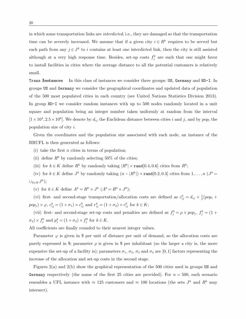
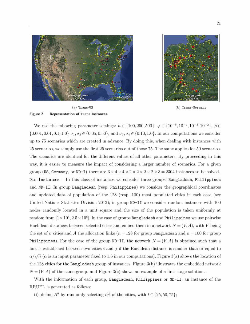
Trans Instances In this class of instances we consider three groups: US, Germany and ND-I. In

groups US and Germany we consider the geographical coordinates and updated data of population

of the 500 most populated cities in each country (see United Nations Statistics Division 2013).

In group ND-I we consider random instances with up to 500 nodes randomly located in a unit

square and population being an integer number taken uniformly at random from the interval

[1×104,2.5×106]. We denote by dij the Euclidean distance between cities i and j, and by popi the

population size of city i.

Given the coordinates and the population size associated with each node, an instance of the

RRUFL is then generated as follows:

(i) take the first n cities in terms of population;

(ii) define R0 by randomly selecting 50% of the cities;

(iii) for k ∈K define Rk by randomly taking |R0| × rand[0.4,0.6] cities from R0;

(iv) for k ∈K define Jk by randomly taking (n−|Rk|)×rand[0.2,0.3] cities from 1, . . . , n (J0 =

∪k∈KJk);

(v) for k ∈K define Ak =Rk× Jk (A0 =R0× J0);

(vi) first- and second-stage transportation/allocation costs are defined as c0ij = dij × 1

2(popi +

popj)×ϕ, ckij = (1 +σ1)× c0ij and rkij = (1 +σ2)× c0

ij for k ∈K;

(vii) first- and second-stage set-up costs and penalties are defined as f0j = ρ× popj, fkj = (1 +

σ3)× f0j and pkj = (1 +σ4)× f0

j for k ∈K.

All coefficients are finally rounded to their nearest integer values.

Parameter ϕ is given in $ per unit of distance per unit of demand, so the allocation costs are

purely expressed in $; parameter ρ is given in $ per inhabitant (so the larger a city is, the more

expensive the set-up of a facility is); parameters σ1, σ2, σ3 and σ4 are [0,1] factors representing the

increase of the allocation and set-up costs in the second stage.

Figures 2(a) and 2(b) show the graphical representation of the 500 cities used in groups US and

Germany respectively (the name of the first 25 cities are provided). For n = 500, each scenario

resembles a UFL instance with ≈ 125 customers and ≈ 100 locations (the sets Jk and Rk may

intersect).

21

(a) Trans-US (b) Trans-Germany

Figure 2 Representation of Trans Instances.

We use the following parameter settings: n ∈ {100,250,500}, ϕ ∈ {10−5,10−4,10−3,10−2}, ρ ∈

{0.001,0.01,0.1,1.0} σ1, σ2 ∈ {0.05,0.50}, and σ3, σ4 ∈ {0.10,1.0}. In our computations we consider

up to 75 scenarios which are created in advance. By doing this, when dealing with instances with

25 scenarios, we simply use the first 25 scenarios out of those 75. The same applies for 50 scenarios.

The scenarios are identical for the different values of all other parameters. By proceeding in this

way, it is easier to measure the impact of considering a larger number of scenarios. For a given

group (US, Germany, or ND-I) there are 3× 4× 4× 2× 2× 2× 2× 3 = 2304 instances to be solved.

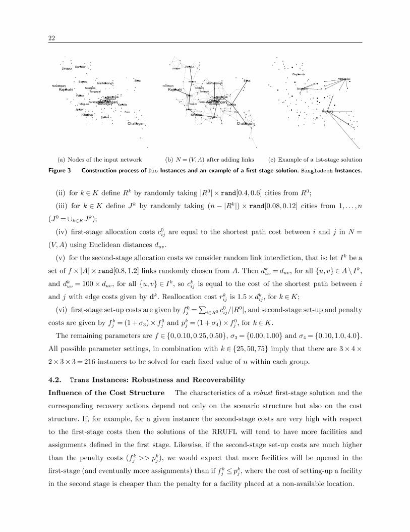
Dis Instances In this class of instances we consider three groups: Bangladesh, Philippines

and ND-II. In group Bangladesh (resp. Philippines) we consider the geographical coordinates

and updated data of population of the 128 (resp. 100) most populated cities in each case (see

United Nations Statistics Division 2013); in group ND-II we consider random instances with 100

nodes randomly located in a unit square and the size of the population is taken uniformly at

random from [1×104,2.5×106]. In the case of groups Bangladesh and Philippines we use pairwise

Euclidean distances between selected cities and embed them in a network N = (V,A), with V being

the set of n cities and A the allocation links (n= 128 for group Bangladesh and n= 100 for group

Philippines). For the case of the group ND-II, the network N = (V,A) is obtained such that a

link is established between two cities i and j if the Euclidean distance is smaller than or equal to

α/√n (α is an input parameter fixed to 1.6 in our computations). Figure 3(a) shows the location of

the 128 cities for the Bangladesh group of instances, Figure 3(b) illustrates the embedded network

N = (V,A) of the same group, and Figure 3(c) shows an example of a first-stage solution.

With the information of each group, Bangladesh, Philippines or ND-II, an instance of the

RRUFL is generated as follows:

(i) define R0 by randomly selecting t% of the cities, with t∈ {25,50,75};

22

(a) Nodes of the input network (b) N = (V,A) after adding links (c) Example of a 1st-stage solution

Figure 3 Construction process of Dis Instances and an example of a first-stage solution. Bangladesh Instances.

(ii) for k ∈K define Rk by randomly taking |R0| × rand[0.4,0.6] cities from R0;

(iii) for k ∈ K define Jk by randomly taking (n − |Rk|) × rand[0.08,0.12] cities from 1, . . . , n

(J0 =∪k∈KJk);

(iv) first-stage allocation costs c0ij are equal to the shortest path cost between i and j in N =

(V,A) using Euclidean distances duv.

(v) for the second-stage allocation costs we consider random link interdiction, that is: let Ik be a

set of f ×|A|×rand[0.8,1.2] links randomly chosen from A. Then dkuv = duv, for all {u, v} ∈A \ Ik,

and dkuv = 100× duv, for all {u, v} ∈ Ik, so ckij is equal to the cost of the shortest path between i

and j with edge costs given by dk. Reallocation cost rkij is 1.5× dkij, for k ∈K;

(vi) first-stage set-up costs are given by f0j =

∑i∈R0 c0

ij/|R0|, and second-stage set-up and penalty

costs are given by fkj = (1 +σ3)× f0j and pkj = (1 +σ4)× f0

j , for k ∈K.

The remaining parameters are f ∈ {0,0.10,0.25,0.50}, σ3 = {0.00,1.00} and σ4 = {0.10,1.0,4.0}.

All possible parameter settings, in combination with k ∈ {25,50,75} imply that there are 3× 4×

2× 3× 3 = 216 instances to be solved for each fixed value of n within each group.

4.2. Trans Instances: Robustness and Recoverability

Influence of the Cost Structure The characteristics of a robust first-stage solution and the

corresponding recovery actions depend not only on the scenario structure but also on the cost

structure. If, for example, for a given instance the second-stage costs are very high with respect

to the first-stage costs then the solutions of the RRUFL will tend to have more facilities and

assignments defined in the first stage. Likewise, if the second-stage set-up costs are much higher

than the penalty costs (fkj >> pkj ), we would expect that more facilities will be opened in the

first-stage (and eventually more assignments) than if fkj ≤ pkj , where the cost of setting-up a facility

in the second stage is cheaper than the penalty for a facility placed at a non-available location.

23

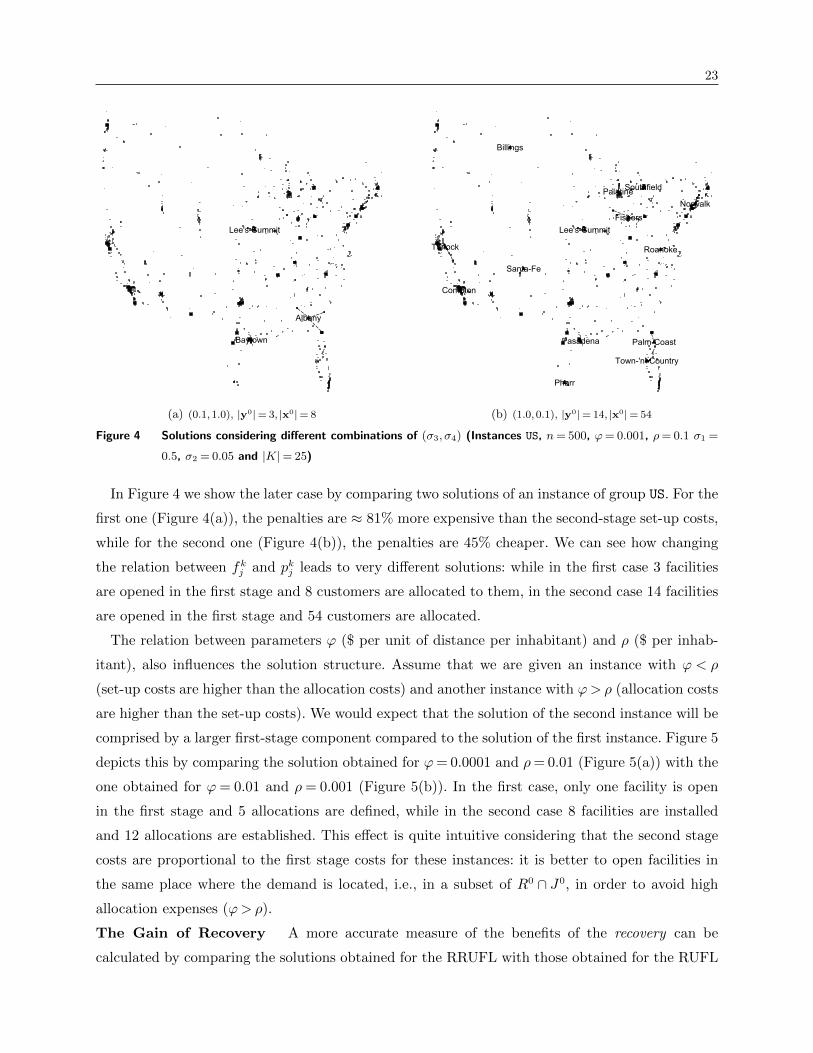
(a) (0.1,1.0), |y0| = 3, |x0| = 8 (b) (1.0,0.1), |y0| = 14, |x0| = 54

Figure 4 Solutions considering different combinations of (σ3, σ4) (Instances US, n= 500, ϕ= 0.001, ρ= 0.1 σ1 =

0.5, σ2 = 0.05 and |K|= 25)

In Figure 4 we show the later case by comparing two solutions of an instance of group US. For the

first one (Figure 4(a)), the penalties are ≈ 81% more expensive than the second-stage set-up costs,

while for the second one (Figure 4(b)), the penalties are 45% cheaper. We can see how changing

the relation between fkj and pkj leads to very different solutions: while in the first case 3 facilities

are opened in the first stage and 8 customers are allocated to them, in the second case 14 facilities

are opened in the first stage and 54 customers are allocated.

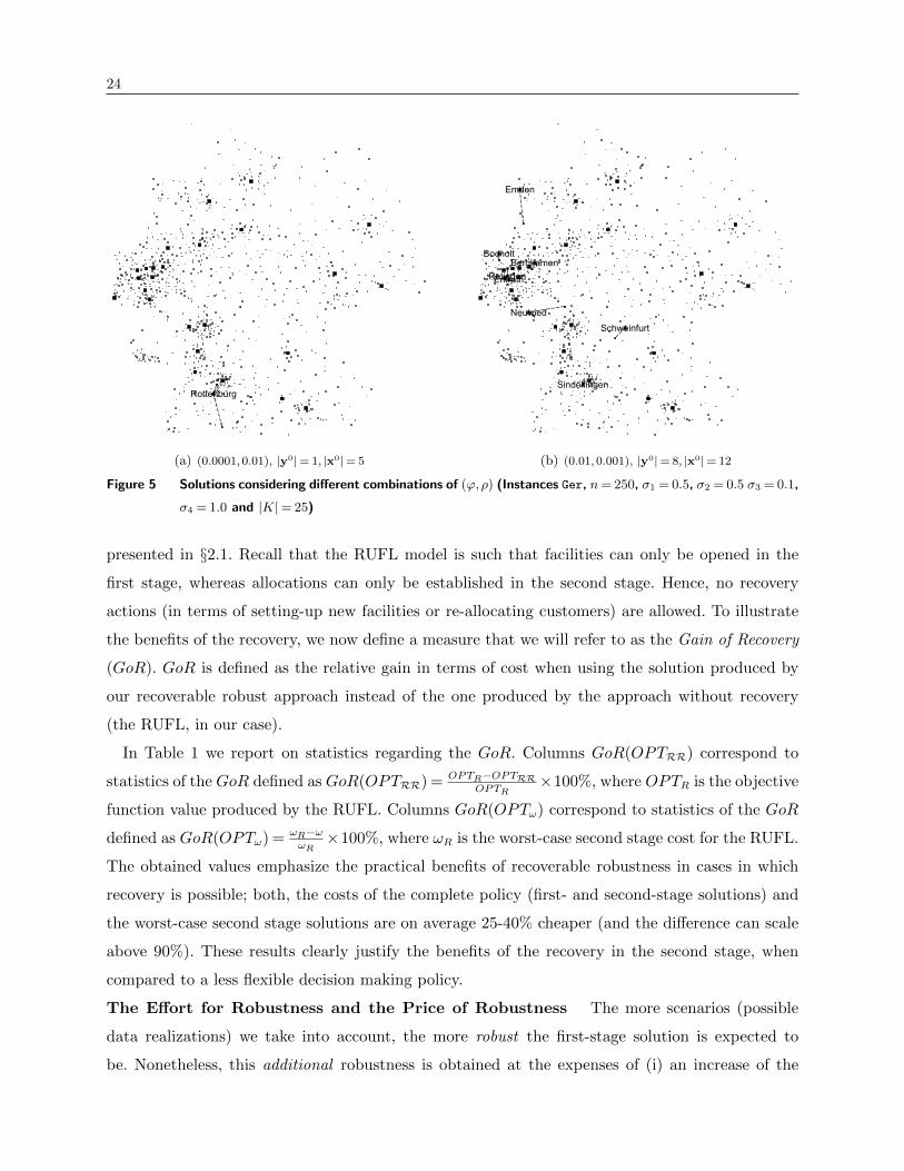
The relation between parameters ϕ ($ per unit of distance per inhabitant) and ρ ($ per inhab-

itant), also influences the solution structure. Assume that we are given an instance with ϕ < ρ

(set-up costs are higher than the allocation costs) and another instance with ϕ> ρ (allocation costs

are higher than the set-up costs). We would expect that the solution of the second instance will be

comprised by a larger first-stage component compared to the solution of the first instance. Figure 5

depicts this by comparing the solution obtained for ϕ= 0.0001 and ρ= 0.01 (Figure 5(a)) with the

one obtained for ϕ= 0.01 and ρ= 0.001 (Figure 5(b)). In the first case, only one facility is open

in the first stage and 5 allocations are defined, while in the second case 8 facilities are installed

and 12 allocations are established. This effect is quite intuitive considering that the second stage

costs are proportional to the first stage costs for these instances: it is better to open facilities in

the same place where the demand is located, i.e., in a subset of R0 ∩ J0, in order to avoid high

allocation expenses (ϕ> ρ).

The Gain of Recovery A more accurate measure of the benefits of the recovery can be

calculated by comparing the solutions obtained for the RRUFL with those obtained for the RUFL

24

(a) (0.0001,0.01), |y0| = 1, |x0| = 5 (b) (0.01,0.001), |y0| = 8, |x0| = 12

Figure 5 Solutions considering different combinations of (ϕ,ρ) (Instances Ger, n= 250, σ1 = 0.5, σ2 = 0.5 σ3 = 0.1,

σ4 = 1.0 and |K|= 25)

presented in §2.1. Recall that the RUFL model is such that facilities can only be opened in the

first stage, whereas allocations can only be established in the second stage. Hence, no recovery

actions (in terms of setting-up new facilities or re-allocating customers) are allowed. To illustrate

the benefits of the recovery, we now define a measure that we will refer to as the Gain of Recovery

(GoR). GoR is defined as the relative gain in terms of cost when using the solution produced by

our recoverable robust approach instead of the one produced by the approach without recovery

(the RUFL, in our case).

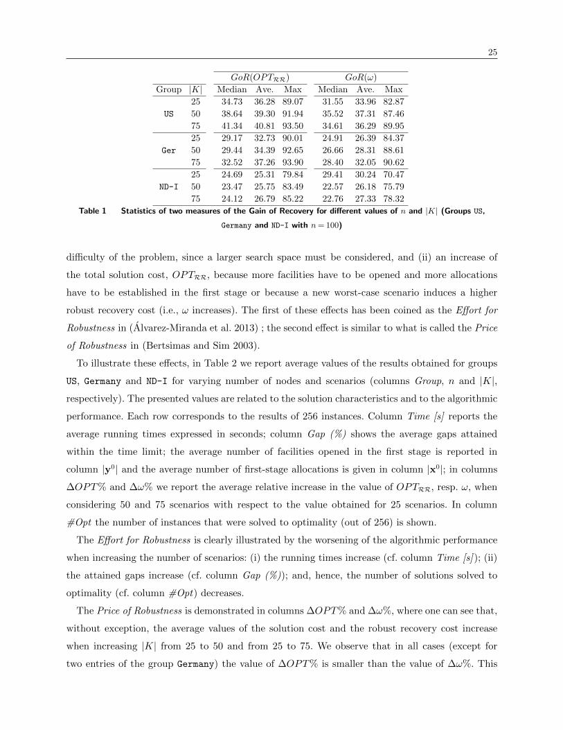
In Table 1 we report on statistics regarding the GoR. Columns GoR(OPTRR) correspond to

statistics of the GoR defined as GoR(OPTRR) = OPTR−OPTRROPTR

×100%, where OPTR is the objective

function value produced by the RUFL. Columns GoR(OPTω) correspond to statistics of the GoR

defined as GoR(OPTω) = ωR−ωωR×100%, where ωR is the worst-case second stage cost for the RUFL.

The obtained values emphasize the practical benefits of recoverable robustness in cases in which

recovery is possible; both, the costs of the complete policy (first- and second-stage solutions) and

the worst-case second stage solutions are on average 25-40% cheaper (and the difference can scale

above 90%). These results clearly justify the benefits of the recovery in the second stage, when

compared to a less flexible decision making policy.

The Effort for Robustness and the Price of Robustness The more scenarios (possible

data realizations) we take into account, the more robust the first-stage solution is expected to

be. Nonetheless, this additional robustness is obtained at the expenses of (i) an increase of the

25

GoR(OPTRR) GoR(ω)

Group |K| Median Ave. Max Median Ave. Max

25 34.73 36.28 89.07 31.55 33.96 82.87

US 50 38.64 39.30 91.94 35.52 37.31 87.46

75 41.34 40.81 93.50 34.61 36.29 89.95

25 29.17 32.73 90.01 24.91 26.39 84.37

Ger 50 29.44 34.39 92.65 26.66 28.31 88.61

75 32.52 37.26 93.90 28.40 32.05 90.62

25 24.69 25.31 79.84 29.41 30.24 70.47

ND-I 50 23.47 25.75 83.49 22.57 26.18 75.79

75 24.12 26.79 85.22 22.76 27.33 78.32

Table 1 Statistics of two measures of the Gain of Recovery for different values of n and |K| (Groups US,

Germany and ND-I with n= 100)

difficulty of the problem, since a larger search space must be considered, and (ii) an increase of

the total solution cost, OPTRR, because more facilities have to be opened and more allocations

have to be established in the first stage or because a new worst-case scenario induces a higher

robust recovery cost (i.e., ω increases). The first of these effects has been coined as the Effort for

Robustness in (Alvarez-Miranda et al. 2013) ; the second effect is similar to what is called the Price

of Robustness in (Bertsimas and Sim 2003).

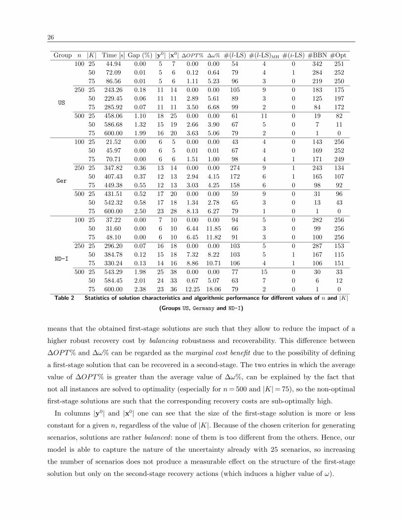
To illustrate these effects, in Table 2 we report average values of the results obtained for groups

US, Germany and ND-I for varying number of nodes and scenarios (columns Group, n and |K|,

respectively). The presented values are related to the solution characteristics and to the algorithmic

performance. Each row corresponds to the results of 256 instances. Column Time [s] reports the

average running times expressed in seconds; column Gap (%) shows the average gaps attained

within the time limit; the average number of facilities opened in the first stage is reported in

column |y0| and the average number of first-stage allocations is given in column |x0|; in columns

∆OPT% and ∆ω% we report the average relative increase in the value of OPTRR, resp. ω, when

considering 50 and 75 scenarios with respect to the value obtained for 25 scenarios. In column

#Opt the number of instances that were solved to optimality (out of 256) is shown.

The Effort for Robustness is clearly illustrated by the worsening of the algorithmic performance

when increasing the number of scenarios: (i) the running times increase (cf. column Time [s]); (ii)

the attained gaps increase (cf. column Gap (%)); and, hence, the number of solutions solved to

optimality (cf. column #Opt) decreases.

The Price of Robustness is demonstrated in columns ∆OPT% and ∆ω%, where one can see that,

without exception, the average values of the solution cost and the robust recovery cost increase

when increasing |K| from 25 to 50 and from 25 to 75. We observe that in all cases (except for

two entries of the group Germany) the value of ∆OPT% is smaller than the value of ∆ω%. This

26

Group n |K| Time [s] Gap (%) |y0| |x0| ∆OPT% ∆ω% #(l-LS) #(l-LS)MH #(i-LS) #BBN #Opt

US

100 25 44.94 0.00 5 7 0.00 0.00 54 4 0 342 251

50 72.09 0.01 5 6 0.12 0.64 79 4 1 284 252

75 86.56 0.01 5 6 1.11 5.23 96 3 0 219 250

250 25 243.26 0.18 11 14 0.00 0.00 105 9 0 183 175

50 229.45 0.06 11 11 2.89 5.61 89 3 0 125 197

75 285.92 0.07 11 11 3.50 6.68 99 2 0 84 172

500 25 458.06 1.10 18 25 0.00 0.00 61 11 0 19 82

50 586.68 1.32 15 19 2.66 3.90 67 5 0 7 11

75 600.00 1.99 16 20 3.63 5.06 79 2 0 1 0

Ger

100 25 21.52 0.00 6 5 0.00 0.00 43 4 0 143 256

50 45.97 0.00 6 5 0.01 0.01 67 4 0 169 252

75 70.71 0.00 6 6 1.51 1.00 98 4 1 171 249

250 25 347.82 0.36 13 14 0.00 0.00 274 9 1 243 134

50 407.43 0.37 12 13 2.94 4.15 172 6 1 165 107

75 449.38 0.55 12 13 3.03 4.25 158 6 0 98 92

500 25 431.51 0.52 17 20 0.00 0.00 59 9 0 31 96

50 542.32 0.58 17 18 1.34 2.78 65 3 0 13 43

75 600.00 2.50 23 28 8.13 6.27 79 1 0 1 0

ND-I

100 25 37.22 0.00 7 10 0.00 0.00 94 5 0 282 256

50 31.60 0.00 6 10 6.44 11.85 66 3 0 99 256

75 48.10 0.00 6 10 6.45 11.82 91 3 0 100 256

250 25 296.20 0.07 16 18 0.00 0.00 103 5 0 287 153

50 384.78 0.12 15 18 7.32 8.22 103 5 1 167 115

75 330.24 0.13 14 16 8.86 10.71 106 4 1 106 151

500 25 543.29 1.98 25 38 0.00 0.00 77 15 0 30 33

50 584.45 2.01 24 33 0.67 5.07 63 7 0 6 12

75 600.00 2.38 23 36 12.25 18.06 79 2 0 1 0

Table 2 Statistics of solution characteristics and algorithmic performance for different values of n and |K|

(Groups US, Germany and ND-I)

means that the obtained first-stage solutions are such that they allow to reduce the impact of a

higher robust recovery cost by balancing robustness and recoverability. This difference between

∆OPT% and ∆ω% can be regarded as the marginal cost benefit due to the possibility of defining

a first-stage solution that can be recovered in a second-stage. The two entries in which the average

value of ∆OPT% is greater than the average value of ∆ω%, can be explained by the fact that

not all instances are solved to optimality (especially for n= 500 and |K|= 75), so the non-optimal

first-stage solutions are such that the corresponding recovery costs are sub-optimally high.

In columns |y0| and |x0| one can see that the size of the first-stage solution is more or less

constant for a given n, regardless of the value of |K|. Because of the chosen criterion for generating

scenarios, solutions are rather balanced : none of them is too different from the others. Hence, our

model is able to capture the nature of the uncertainty already with 25 scenarios, so increasing

the number of scenarios does not produce a measurable effect on the structure of the first-stage

solution but only on the second-stage recovery actions (which induces a higher value of ω).

27

4.3. Trans Instances: Algorithmic Performance

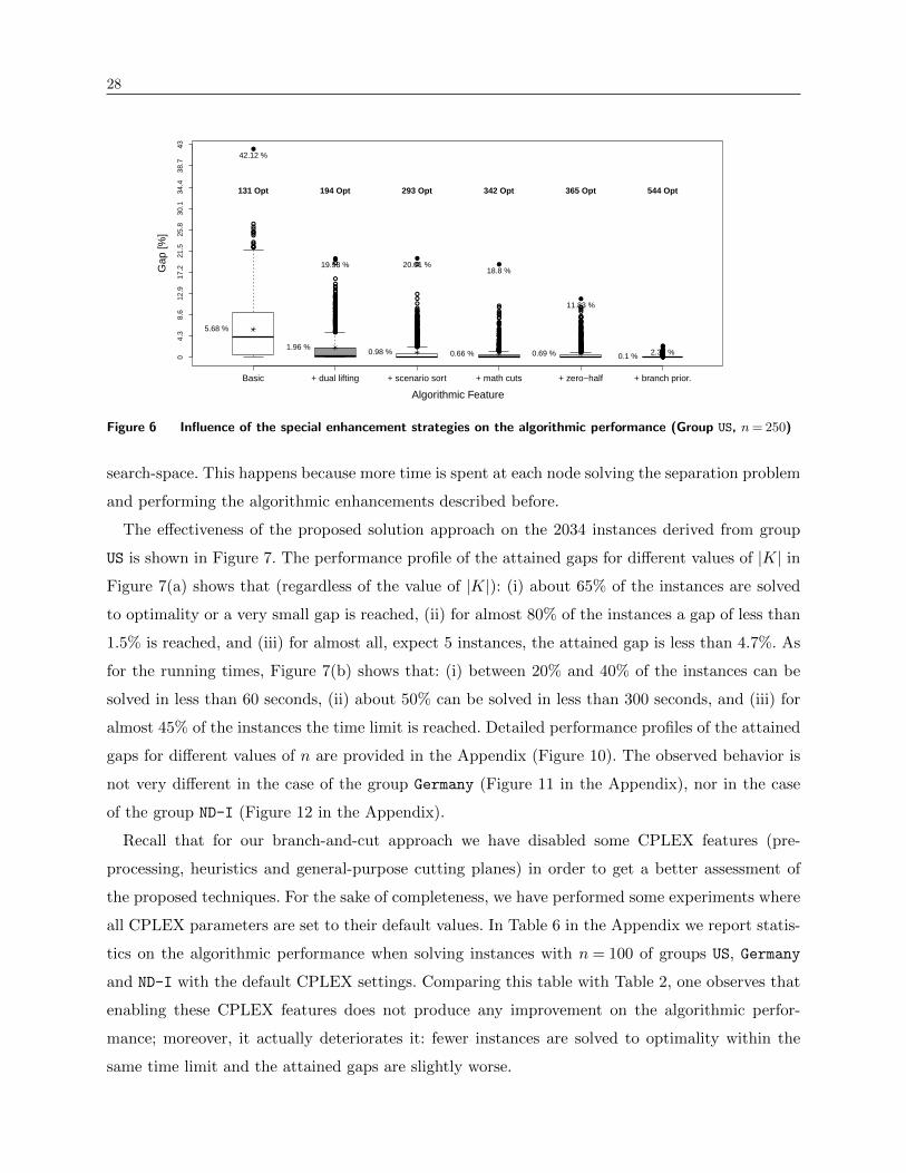
Assessment of Algorithmic Enhancements In §3 we have described several enhance-

ments for our algorithm: cut strengthening based on dual-lifting, scenario sorting, zero-half cuts,

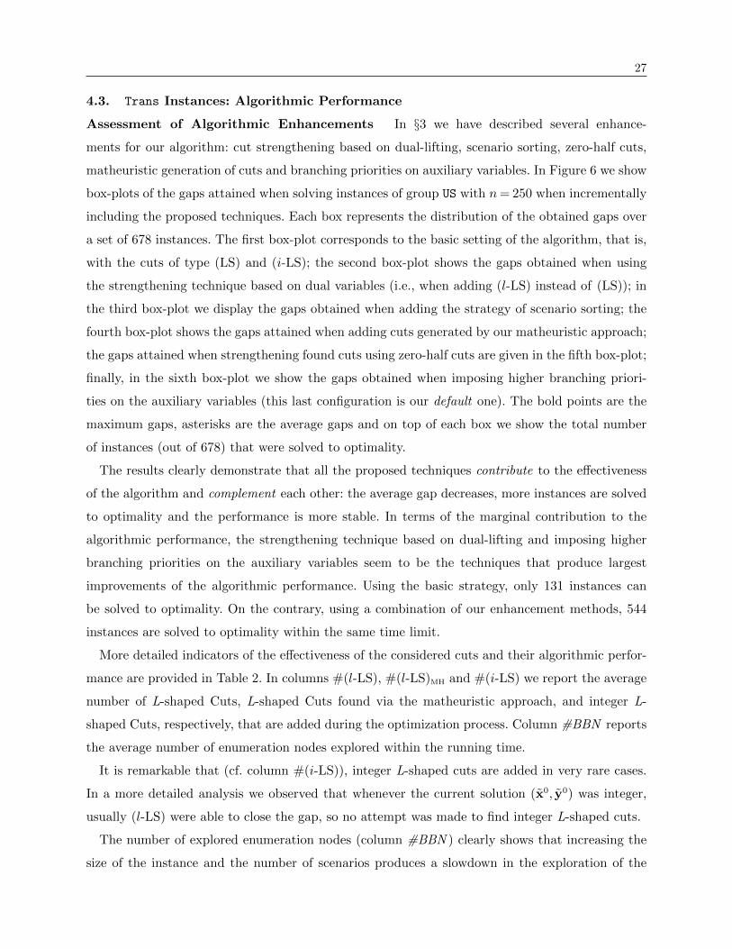
matheuristic generation of cuts and branching priorities on auxiliary variables. In Figure 6 we show

box-plots of the gaps attained when solving instances of group US with n= 250 when incrementally

including the proposed techniques. Each box represents the distribution of the obtained gaps over

a set of 678 instances. The first box-plot corresponds to the basic setting of the algorithm, that is,

with the cuts of type (LS) and (i-LS); the second box-plot shows the gaps obtained when using

the strengthening technique based on dual variables (i.e., when adding (l-LS) instead of (LS)); in

the third box-plot we display the gaps obtained when adding the strategy of scenario sorting; the

fourth box-plot shows the gaps attained when adding cuts generated by our matheuristic approach;

the gaps attained when strengthening found cuts using zero-half cuts are given in the fifth box-plot;

finally, in the sixth box-plot we show the gaps obtained when imposing higher branching priori-

ties on the auxiliary variables (this last configuration is our default one). The bold points are the

maximum gaps, asterisks are the average gaps and on top of each box we show the total number

of instances (out of 678) that were solved to optimality.

The results clearly demonstrate that all the proposed techniques contribute to the effectiveness

of the algorithm and complement each other: the average gap decreases, more instances are solved

to optimality and the performance is more stable. In terms of the marginal contribution to the

algorithmic performance, the strengthening technique based on dual-lifting and imposing higher

branching priorities on the auxiliary variables seem to be the techniques that produce largest

improvements of the algorithmic performance. Using the basic strategy, only 131 instances can

be solved to optimality. On the contrary, using a combination of our enhancement methods, 544

instances are solved to optimality within the same time limit.

More detailed indicators of the effectiveness of the considered cuts and their algorithmic perfor-

mance are provided in Table 2. In columns #(l-LS), #(l-LS)MH and #(i-LS) we report the average

number of L-shaped Cuts, L-shaped Cuts found via the matheuristic approach, and integer L-

shaped Cuts, respectively, that are added during the optimization process. Column #BBN reports

the average number of enumeration nodes explored within the running time.

It is remarkable that (cf. column #(i-LS)), integer L-shaped cuts are added in very rare cases.

In a more detailed analysis we observed that whenever the current solution (x0, y0) was integer,

usually (l-LS) were able to close the gap, so no attempt was made to find integer L-shaped cuts.

The number of explored enumeration nodes (column #BBN ) clearly shows that increasing the

size of the instance and the number of scenarios produces a slowdown in the exploration of the

28

●

●

●

●

●

●

●●

●●

●

●

●

●

●

●

●●

●

●

●

●

●●

●

●

●

●

●●

●●●●

●

●

●

●●

●

●

●

●

●

●

●●●

●●

●●

●●

●

●

●●●●

●

●

●

●

●

●

●

●

●

●

●

●

●

●

●

●

●

●●●

●

●

●

●

●

●

●

●

●●

●

●

●●

●

●

●

●

●

●

●

●●●

●

●

●●●

●

●

●

●●●

●

●

●

●

●

●

●

●

●

●●●

●

●

●

●

●●

●●

●

●

●●

●

●●

●

●●●

●

●

●

●

●●

●

●

●●

●

●

●

●●●●

●

●

●●●●●●●●●

●●●●●●●

●

●

●

●●

●●

●

●

●

●

●●

●

●

●

●

●

●

●●●●●

●

●

●

●●●

●

●

●

●

●

●

●

●

●

●

●●

●

●

●●

●●●●

●

●

●

●

●

●●●

●

●●

●●●

●

●

●

●

●

●

●

●

●

●

●

●●●●●●

●●

●

●●

●●●●●

●

●

●

●

●●

●

●

●

●

●

●

●

●

●

●

●

●●●●●●●

●

●

●

●

●

●●●●

●●●●●●●●

●●

●●●●●●●

●●

●●●●

●

●

●●●●●

●●●●●●

●●●

●

●●●●●●●●

●

●●

●

●

●

●●●●●●●●●●

●

●

●

●●●

●

●

●●●●●

●

●●

●

●

●●

●●●

●●●●●

●

●●

●

●●●

●●●●●●

●

●

●●●

●

●

●

●

●

●

●

●

●

●●

●

●●●

●

●

●

●

●

●

●

●●●

●

●

●

●

●

●●●●●

●

●

●

●

●●

●●●

●●

●

●

●●●●

●●●

●●●

●●●●●●●●

●●●

●●●●●●●●●●●●●●●●●●●●●●●●●●●●●●●●●●●●●●●●●●●●●●●●●●●●●●●●●●●●

●●●●●●●●●●●●●●●●●●●●●●●●●●●●●●●

●●●●●●●●●●●●●●●●●

●

●●●●●●●●●●●●

●

●●●

Algorithmic Feature

Gap

[%]

Basic + dual lifting + scenario sort + math cuts + zero−half + branch prior.

04.

38.

612

.917

.221

.525

.830

.134

.438

.743

5.68 %

●

42.12 %

131 Opt

1.96 %

●

19.98 %

194 Opt

0.98 %

●

20.01 %

293 Opt

0.66 %

●

18.8 %

342 Opt

0.69 %

●

11.83 %

365 Opt

0.1 %

●

2.32 %

544 Opt

Figure 6 Influence of the special enhancement strategies on the algorithmic performance (Group US, n= 250)

search-space. This happens because more time is spent at each node solving the separation problem

and performing the algorithmic enhancements described before.

The effectiveness of the proposed solution approach on the 2034 instances derived from group

US is shown in Figure 7. The performance profile of the attained gaps for different values of |K| in

Figure 7(a) shows that (regardless of the value of |K|): (i) about 65% of the instances are solved

to optimality or a very small gap is reached, (ii) for almost 80% of the instances a gap of less than

1.5% is reached, and (iii) for almost all, expect 5 instances, the attained gap is less than 4.7%. As

for the running times, Figure 7(b) shows that: (i) between 20% and 40% of the instances can be

solved in less than 60 seconds, (ii) about 50% can be solved in less than 300 seconds, and (iii) for

almost 45% of the instances the time limit is reached. Detailed performance profiles of the attained

gaps for different values of n are provided in the Appendix (Figure 10). The observed behavior is

not very different in the case of the group Germany (Figure 11 in the Appendix), nor in the case

of the group ND-I (Figure 12 in the Appendix).

Recall that for our branch-and-cut approach we have disabled some CPLEX features (pre-

processing, heuristics and general-purpose cutting planes) in order to get a better assessment of

the proposed techniques. For the sake of completeness, we have performed some experiments where

all CPLEX parameters are set to their default values. In Table 6 in the Appendix we report statis-

tics on the algorithmic performance when solving instances with n = 100 of groups US, Germany

and ND-I with the default CPLEX settings. Comparing this table with Table 2, one observes that

enabling these CPLEX features does not produce any improvement on the algorithmic perfor-

mance; moreover, it actually deteriorates it: fewer instances are solved to optimality within the

same time limit and the attained gaps are slightly worse.

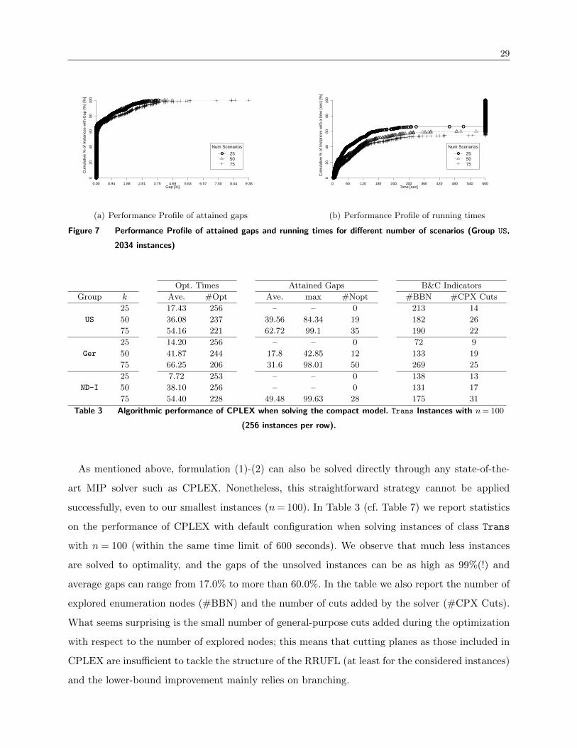
29

Gap [%]

Cum

ulat

ive

% o

f Ins

tanc

es w

ith G

ap (

%)

[%]

●●●●●●●●●●●●●●●●●●●●●●●●●●●●●●●●●●●●●●●●●●●●●●●●●●●●●●●●●●●●●●●●●●●●●●●●●●●●●●●●●●●●●●●●●●●●●●●●●●●●●●●●●●●●●●●●●●●●●●●●●●●●●●●●●●●●●●●●●●●●●●●●●●●●●●●●●●●●●●●●●●●●●●●●●●●●●●●●●●●●●●●●●●●●●●●●●●●●●●●●●●●●●●●●●●●●●●●●●●●●●●●●●●●●●●●●●●●●●●●●●●●●●●●●●●●●●●●●●●●●●●●●●●●●●●●●●●●●●●●●●●●●●●●●●●●●●●●●●●●●●●●●●●●●●●●●●●●●●●●●●●●●●●●●●●●●●●●●●●●●●●●●●●●●●●●●●●●●●●●●●●●●●●●●●●●●●●●●●●●●●●●●●●●●●●●●●●●●●●●●●●●●●●●●●●●●●●●●●●●●●●●●●●●●●●●●●●●●●●●●●●●●●●●●●●●●●●●●●●●●●●●●●●●●●●●●●●●●●●●●●●●●●●●●●●●●●●●●●●●●●●●●●●●●●●●●●●●●●●●●●●●●●●●●●●●●●●●●●●●●●●●●●●●●●●●●●●●●●●●●●

●●●●●●●●●●●●●●●●●●●●●●●●●●●●●●●●●●

●●●●●●●●●●●●●●●●●●●●●●●●●●●●●●●●●●

●●●●●●●●●●●●●●●●●●●●●●●●●●●●●●●●●●

●●●●●●●●●●●●●●●●●●●●●●●●●●●●●●●●●●

●●●●●●●●●●●●●●●●●●●●●●●●●●●●●●●●●●

●●●●●●●●●●●●●●●●●●●●●●●●●●●●●●●● ●●●●●

0.00 0.94 1.88 2.81 3.75 4.69 5.63 6.57 7.50 8.44 9.38

020

4060

8010

0

●

Num Scenarios

255075

(a) Performance Profile of attained gaps

Time [sec]

Cum

ulat

ive

% o

f Ins

tanc

es w

ith a

tim

e (s

ec)

[%]

●●●●●●●●●●●●●●●●●●●●●●●●●●●●●●●●●●●●●●●●●●●●●●●●●●●●●●●●●●●●●●●●●●●●●●●●●●●●●●●●●●●●●●●●●●●●●●●●●●●●●●●●●●●●●●●●●●●●●●●●●●●●●●●●●●●●●●●●●●●●●●●●●●●●●●●●●●●●●●●●●●●●●●●●●●●●●●●●●●●●●●●●●●●●●●●●●●●●●●●●●●●●●●●●●●●●●●●●●●●●●●●●●●●●●●●●●●●●●●●●●●●●●●●●●●●●●●●●●●●●●●●●●●●●●●●●●●●●●●●●●●●●●●●●●●●●●●●●●●●●●●●●●●●●●●●●●●●●●●●●●●●

●●●●●●●●●●●●●●●●●●●●●●●●●●●●●●●●●●

●●●●●●●●●●●●●●●●●●●●●●●●●●●●●●●●●●

●●●●●●●●●●●●●●●●●●●●●●●●●●●●●●●●●●

●●●●●●●●●●●●●●●●●●●●●●●●●●●●●●●●●●

●●●●●●●●●●●●●●●●●●●●● ●●●●●●●●●●●●●●●●●●●●●●●●● ● ● ● ●●●●●●●●●●●●●●●●●●●●●●●●●●●●●●●●●●●●●●●●●●●●●●●●●●●●●●●●●●●●●●●●●●●●●●●●●●●●●●●●●●●●●●●●●●●●●●●●●●●●●●●●●●●●●●●●●●●●●●●●●●●●●●●●●●●●●●●●●●●●●●●●●●●●●●●●●●●●●●●●●●●●●●●●●●●●●●●●●●●●●●●●●●●●●●●●●●●●●●●●●●●●●●●●●●●●●●●●●●●●●●●●●●●●●●●●●●●●●●●●●●●●●●●●●●●●●●●●●●●●

0 60 120 180 240 300 360 420 480 540 600

020

4060

8010

0

●

Num Scenarios

255075

(b) Performance Profile of running times

Figure 7 Performance Profile of attained gaps and running times for different number of scenarios (Group US,

2034 instances)

Opt. Times Attained Gaps B&C Indicators

Group k Ave. #Opt Ave. max #Nopt #BBN #CPX Cuts

US

25 17.43 256 – – 0 213 14

50 36.08 237 39.56 84.34 19 182 26

75 54.16 221 62.72 99.1 35 190 22

Ger

25 14.20 256 – – 0 72 9

50 41.87 244 17.8 42.85 12 133 19

75 66.25 206 31.6 98.01 50 269 25

ND-I

25 7.72 253 – – 0 138 13

50 38.10 256 – – 0 131 17

75 54.40 228 49.48 99.63 28 175 31

Table 3 Algorithmic performance of CPLEX when solving the compact model. Trans Instances with n= 100

(256 instances per row).

As mentioned above, formulation (1)-(2) can also be solved directly through any state-of-the-

art MIP solver such as CPLEX. Nonetheless, this straightforward strategy cannot be applied

successfully, even to our smallest instances (n= 100). In Table 3 (cf. Table 7) we report statistics

on the performance of CPLEX with default configuration when solving instances of class Trans

with n = 100 (within the same time limit of 600 seconds). We observe that much less instances

are solved to optimality, and the gaps of the unsolved instances can be as high as 99%(!) and

average gaps can range from 17.0% to more than 60.0%. In the table we also report the number of

explored enumeration nodes (#BBN) and the number of cuts added by the solver (#CPX Cuts).

What seems surprising is the small number of general-purpose cuts added during the optimization

with respect to the number of explored nodes; this means that cutting planes as those included in

CPLEX are insufficient to tackle the structure of the RRUFL (at least for the considered instances)

and the lower-bound improvement mainly relies on branching.

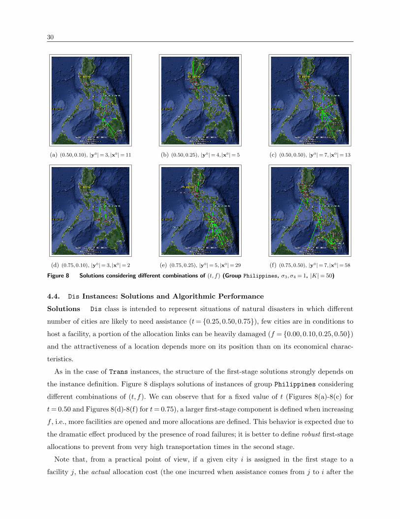
30

(a) (0.50,0.10), |y0| = 3, |x0| = 11 (b) (0.50,0.25), |y0| = 4, |x0| = 5 (c) (0.50,0.50), |y0| = 7, |x0| = 13

(d) (0.75,0.10), |y0| = 3, |x0| = 2 (e) (0.75,0.25), |y0| = 5, |x0| = 29 (f) (0.75,0.50), |y0| = 7, |x0| = 58

Figure 8 Solutions considering different combinations of (t, f) (Group Philippines, σ3, σ4 = 1, |K|= 50)

4.4. Dis Instances: Solutions and Algorithmic Performance

Solutions Dis class is intended to represent situations of natural disasters in which different

number of cities are likely to need assistance (t= {0.25,0.50,0.75}), few cities are in conditions to

host a facility, a portion of the allocation links can be heavily damaged (f = {0.00,0.10,0.25,0.50})

and the attractiveness of a location depends more on its position than on its economical charac-

teristics.

As in the case of Trans instances, the structure of the first-stage solutions strongly depends on

the instance definition. Figure 8 displays solutions of instances of group Philippines considering

different combinations of (t, f). We can observe that for a fixed value of t (Figures 8(a)-8(c) for

t= 0.50 and Figures 8(d)-8(f) for t= 0.75), a larger first-stage component is defined when increasing

f , i.e., more facilities are opened and more allocations are defined. This behavior is expected due to

the dramatic effect produced by the presence of road failures; it is better to define robust first-stage

allocations to prevent from very high transportation times in the second stage.

Note that, from a practical point of view, if a given city i is assigned in the first stage to a

facility j, the actual allocation cost (the one incurred when assistance comes from j to i after the

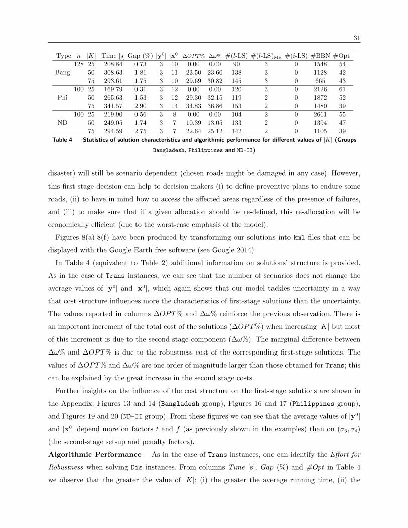
31

Type n |K| Time [s] Gap (%) |y0| |x0| ∆OPT% ∆ω% #(l-LS) #(l-LS)MH #(i-LS) #BBN #Opt

Bang128 25 208.84 0.73 3 10 0.00 0.00 90 3 0 1548 54

50 308.63 1.81 3 11 23.50 23.60 138 3 0 1128 42

75 293.61 1.75 3 10 29.69 30.82 145 3 0 665 43

Phi100 25 169.79 0.31 3 12 0.00 0.00 120 3 0 2126 61

50 265.63 1.53 3 12 29.30 32.15 119 2 0 1872 52

75 341.57 2.90 3 14 34.83 36.86 153 2 0 1480 39

ND100 25 219.90 0.56 3 8 0.00 0.00 104 2 0 2661 55

50 249.05 1.74 3 7 10.39 13.05 133 2 0 1394 47

75 294.59 2.75 3 7 22.64 25.12 142 2 0 1105 39

Table 4 Statistics of solution characteristics and algorithmic performance for different values of |K| (Groups

Bangladesh, Philippines and ND-II)

disaster) will still be scenario dependent (chosen roads might be damaged in any case). However,

this first-stage decision can help to decision makers (i) to define preventive plans to endure some

roads, (ii) to have in mind how to access the affected areas regardless of the presence of failures,

and (iii) to make sure that if a given allocation should be re-defined, this re-allocation will be

economically efficient (due to the worst-case emphasis of the model).

Figures 8(a)-8(f) have been produced by transforming our solutions into kml files that can be

displayed with the Google Earth free software (see Google 2014).

In Table 4 (equivalent to Table 2) additional information on solutions’ structure is provided.

As in the case of Trans instances, we can see that the number of scenarios does not change the

average values of |y0| and |x0|, which again shows that our model tackles uncertainty in a way

that cost structure influences more the characteristics of first-stage solutions than the uncertainty.

The values reported in columns ∆OPT% and ∆ω% reinforce the previous observation. There is

an important increment of the total cost of the solutions (∆OPT%) when increasing |K| but most

of this increment is due to the second-stage component (∆ω%). The marginal difference between

∆ω% and ∆OPT% is due to the robustness cost of the corresponding first-stage solutions. The

values of ∆OPT% and ∆ω% are one order of magnitude larger than those obtained for Trans; this

can be explained by the great increase in the second stage costs.

Further insights on the influence of the cost structure on the first-stage solutions are shown in

the Appendix: Figures 13 and 14 (Bangladesh group), Figures 16 and 17 (Philippines group),

and Figures 19 and 20 (ND-II group). From these figures we can see that the average values of |y0|

and |x0| depend more on factors t and f (as previously shown in the examples) than on (σ3, σ4)

(the second-stage set-up and penalty factors).

Algorithmic Performance As in the case of Trans instances, one can identify the Effort for

Robustness when solving Dis instances. From columns Time [s], Gap (%) and #Opt in Table 4

we observe that the greater the value of |K|: (i) the greater the average running time, (ii) the

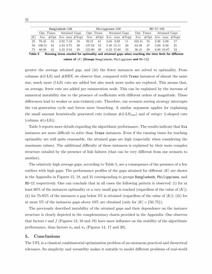
32

Bangladesh-128 Philippines-100 ND-II-100

Opt. Times Attained Gaps Opt. Times Attained Gaps Opt. Times Attained Gaps

|K| Ave. #Opt Ave. max #Nopt Ave. #Opt Ave. max #Nopt Ave. #Opt Ave. max #Nopt

25 78.45 54 2.92 7.43 18 92.21 61 2.04 3.93 11 102.41 55 2.38 5.09 17

50 100.51 42 4.33 9.75 30 137.03 52 5.48 15.11 20 62.38 47 5.00 9.20 25

75 86.98 43 4.33 9.94 29 122.90 39 6.32 15.60 33 36.16 39 6.00 10.87 33

Table 5 Running times needed for optimality and attained gaps when reaching the time limit for different

values of |K| (Groups Bangladesh, Philippines and ND-II)

greater the average attained gap, and (iii) the fewer instances are solved to optimality. From

columns #(l-LS) and #BBN, we observe that, compared with Trans instances of almost the same

size, much more (l-LS) cuts are added but also much more nodes are explored. This means that,

on average, fewer cuts are added per enumeration node. This can be explained by the increase of

numerical instability due to the presence of coefficients with different orders of magnitude. These

differences lead to weaker or non-violated cuts. Therefore, our scenario sorting strategy interrupts

the cut-generation cycle and forces more branching. A similar argument applies for explaining

the small amount heuristically generated cuts (column #(l-LS)MH) and of integer L-shaped cuts

(column #(i-LS)).

Table 5 reports more details regarding the algorithmic performance. The results indicate that Dis

instances are more difficult to solve than Trans instances. Even if the running times for reaching

optimality are still quite reasonable, the attained gaps are high (especially when considering the

maximum values). The additional difficulty of these instances is explained by their more complex

structure entailed by the presence of link failures (that can be very different from one scenario to

another).

The relatively high average gaps, according to Table 5, are a consequence of the presence of a few

outliers with high gaps. The performance profiles of the gaps attained for different |K| are shown

in the Appendix in Figures 15, 18, and 21 corresponding to groups Bangladesh, Philippines, and

ND-II respectively. One can conclude that in all cases the following pattern is observed: (i) for at

least 60% of the instances optimality or a very small gap is reached (regardless of the value of |K|);(ii) for 75-85% of the instances a gap below 5% is attained (regardless of the value of |K|); (iii) for

at most 5% of the instances gaps above 10% are obtained (only for |K|= {50,75}).The previously described instability of the attained gaps and their dependence on the instance

structure is clearly depicted in the complementary charts provided in the Appendix. One observes

that factors t and f (Figures 13, 16 and 19) have more influence on the stability of the algorithmic

performance, than factors σ3 and σ4 (Figures 14, 17 and 20).

5. Conclusions

The UFL is a classical combinatorial optimization problem of an enormous practical and theoretical

relevance. Its simplicity and versatility makes it suitable to model different problems of real-world

33

decision making. Nonetheless, when truly implementable solutions are sought, the consideration of

uncertainty is unavoidable. For the UFL under different sources of uncertainty, we applied a new

recoverable robust optimization approach (RRO) that falls within the framework of 2SRO. In this

new concept, a robust solution is sought such that it can be recovered (i.e., rendered feasible using a

limited set of recovery actions) once the uncertainty is revealed in a second stage. For the resulting

problem, RRUFL, we designed an algorithmic framework based on Benders decomposition and we

included several tailored enhancements to improve its performance.

The proposed algorithm was extensively tested on more than 7500 realistic instances divided into

two groups. The results show the efficacy of the algorithm to find good quality solutions within

a short running time. Moreover, the results demonstrate the strong influence of the instance cost

structure on both the algorithmic performance and solution characteristics. Our computational

study also illustrates how robustness and recoverability are expressed in the structure of optimal

solutions, and it demonstrates the benefits of RRO when compared to a RO model without recovery.

Finally, the obtained results indicate that solving the RRUFL is a not an easy task for general

purpose MIP solvers. To cope with the size of realistic instances, it is inevitable to use more

sophisticated decomposition techniques, like the one presented in this study.

ReferencesD. Adjiashvili. Structural Robustness in Combinatorial Optimization. PhD thesis, ETH ZURICH, 2012.

M. Albareda-Sambola, E. Fernandez, and F. Saldanha-da Gama. The Facility Location problem withBernoulli demands. Omega, 39(3):335–345, 2011.

M. Albareda-Sambola, A. Alonso-Ayuso, L. Escudero, E. Fernandez, and C. Pizarro. Fix-and-relax-coordination for a multi-period location-allocation problem under uncertainty. Computers & OR, 40(12):2878–2892, 2013.

S. Alumur, S. Nickel, and F. Saldanha-da Gama. Hub location under uncertainty. Transportation ResearchPart B: Methodological, 46(4):529–543, 2012.

E. Alvarez-Miranda, I. Ljubic, S. Raghavan, and P. Toth. The recoverable robust two-level network designproblem. Submitted to INFORMS J. on Computing, 2013.

G. Andreello, A. Caprara, and M. Fischetti. Embedding {0,1/2}-cuts in a branch-and-cut framework: Acomputational study. INFORMS Journal on Computing, 19:229–238, 2007.

I. Averbakh. The minmax relative regret median problem on networks. INFORMS Journal on Computing,17(4):451–461, 2005.

A. Ben-Tal, A. Goryashko, E. Guslitzer, and A. Nemirovski. Adjustable robust solutions of uncertain linearprograms. Mathematical Programming, Series A(99):351–376, 2004.

A. Ben-Tal, L. El-Ghaoui, and A. Nemirovski, editors. Robust Optimization. Series in Applied Mathematics.Princeton, 1st edition, 2010.

D. Bertsimas and M. Sim. Robust discrete optimization and network flows. Mathematical Programming,Series B(98):49–71, 2003.

D. Bertsimas and M. Sim. The price of robustness. Operations Research, 52(1):35–53, 2004.

J. Birge and F. Louveaux. Introduction to Stochastic Programming. Series in Operations Research andFinancial Engineering. Springer, 2nd edition, 2011.

34

C. Busing. Recoverable robust shortest path problems. Networks, 59(1):181–189, 2012.

C. Busing, A. Koster, and M. Kutschka. Recoverable robust knapsacks: the discrete scenario case. Opti-mization Letters, 5(3):379–392, 2011.

V. Cacchiani, A. Caprara, L. Galli, L. Kroon, and G. Maroti. Recoverable robustness for railway rollingstock planning. In M. Fischetti and P. Widmayer, editors, Proceedings of ATMOS 2008, volume 9 ofOpenAccess Series in Informatics. Schloss Dagstuhl, 2008.

A. Caprara and M. Fischetti. {0, 12}-Chvatal-Gomory cuts. Mathematical Programming, 74:221–235, 1996.

S. Cicerone, G. Di Stefano, M. Schachtebeck, and A. Schobel. Multi-stage recovery robustness for optimiza-tion problems: A new concept for planning under disturbances. Information Sciences, 190:107–126,2012.

G. Cornuejols, G. Nemhauser, and L. Wolsey. The uncapacitated facility location problem. In P. Mirchandaniand R. Francis, editors, Discrete Location Theory. Wiley-Interscience, 1990.

T. Cui, Y. Ouyang, and Z. Shen. Reliable facility location design under the risk of disruptions. OperationsResearch, 58(4):998–1011, 2010.

G. D’Angelo, G. Di Stefano, A. Navarra, and C. Pinotti. Recoverable robust timetables: An algorithmicapproach on trees. IEEE Transactions on Computers, 60(3):433–446, 2011.

M. Daskin. Network and Discrete Location: Models, Algorithms, and Applications. Wiley, 2nd edition, 2013.

DDM. Department of Disaster Management of Bangladesh, Ministry of Disaster Management and Relief,Government of the Republic Bangladesh, 2014. URL http://http://www.ddm.gov.bd/flood.php/.

H. A. Eiselt and V. Marianov, editors. Foundations of Location Analysis, volume 155 of International Seriesin Operations Research & Management Science. Springer, 2011.

M. Fischetti and A. Lodi. Local branching. Mathematical Programming, 98(1–3):23–47, 2003.

Y. Gao. Uncertain models for single facility location problems on networks. Applied Mathematical Modelling,36(6):2592 – 2599, 2012.

N. Gılpinar, D. Pachamanova, and E. Canakoglu. Robust strategies for facility location under uncertainty.European Journal of Operational Research, 225(1):21–35, 2013.

Google. Google Earth, 2014. URL http://www.google.com/intl/en/earth/.

R. Hassin, R. Ravi, and F. Salman. Facility location on a network with unreliable links. In Proceedings ofINOC 2009. University of Pisa, 2009.

P. Kouvelis and G. Yu, editors. Robust discrete optimization and its applications. Nonconvex Optimizationand its Applications. Kluwer Academic Publishers, 1st edition, 1997.

A. Kuehn and M. Hamburger. A heuristic program for locating warehouses. Management Science, 9(4):643–666, 1963.

G. Laporte and F. Louveaux. The integer L-shaped method for stochastic integer programs with completerecourse. Operations Research Letters, 13(3):133–142, 1993.

A. Letchford and S. Miller. Fast bounding procedures for large instances of the simple plant location problem.Computers & Operations Research, 39(5):985–990, 2012.

Q. Li, B. Zeng, and A. Savachkin. Reliable facility location design under disruptions. Computers & OR, 40(4):901–909, 2013.

C. Liebchen, M. Lubbecke, R. Mohring, and S. Stiller. Recoverable robustness. Technical Report ARRIVAL-TR-0066, ARRIVAL Project, 2007.

C. Liebchen, M. Lubbecke, R. Mohring, and S. Stiller. The concept of recoverable robustness, linear pro-gramming recovery, and railway applications. In R. Ahuja, R. Mohring, and C. Zaroliagis, editors,Robust and Online Large-Scale Optimization, volume 5868 of LNCS, pages 1–/27. Springer, 2009.

I. Ljubic, P. Mutzel, and B. Zey. Stochastic survivable network design problems. Electronic Notes in DiscreteMathematics, 41:245–252, 2013.

35

T. Magnanti and R. Wong. Accelerating Benders decomposition: Algorithmic enhancement and modelselection criteria. Operations Research, 29(3):464–484, 1981.

PAGASA. Philippine Atmospheric, Geophysical and Astronomical Services Administration, Department ofScience and Technology, Republic of the Philippines, 2014. URL http://web.pagasa.dost.gov.ph/.

F. Perez-Galarce, E. Alvarez-Miranda, A. Candia, and P. Toth. On exact solutions for the Minmax Regretspanning tree problem. Forthcoming in Computers & OR, 2014. URL http://dx.doi.org/10.1016/j.cor.2014.02.007.

R. Ravi and A. Sinha. Hedging uncertainty: Approximation algorithms for stochastic optimization problems.Mathematical Programming, 108(1):97–114, 2006.

W. Rei, J-F. Cordeau, M. Gendreau, and P. Soriano. Accelerating Benders decomposition by local branching.INFORMS Journal on Computing, 21(2):333–345, 2009.

Z. Shen, R. Zhan, and J. Zhang. The reliable facility location problem: Formulations, heuristics, and approx-imation algorithms. INFORMS Journal on Computing, 23(3):470–482, 2011.

L. Snyder. Facility location under uncertainty: a review. IIE Transactions, 38(7):547–564, 2006.

L. Snyder and M. Daskin. Reliability models for facility location: The expected failure cost case. Trans-portation Science, 39(3):400–416, 2005.

L. Snyder and M. Daskin. Stochastic p-robust location problems. IIE Transactions, 38(11):971–985, 2006.

United Nations Statistics Division. UNSD Statistical Databases, 2013. URL http://millenniumindicators.un.org/unsd/databases.htm.

R. Van Slyke and R. Wets. L-shaped linear programs with applications to optimal control and stochasticprogramming. SIAM Journal of Applied Mathematics, 17(4):638–663, 1967.

V. Verter. Uncapacitated and capacitated facility location problems. In H. A. Eiselt and V. Marianov,editors, Foundations of Location Analysis, volume 155 of International Series in Operations Research& Management Science, pages 25–37. Springer, 2011.

L. Zhao and B. Zeng. An exact algorithm for two-stage robust optimization with mixed integer recourseproblems. Tech. Report - University of South Florida, 2012.

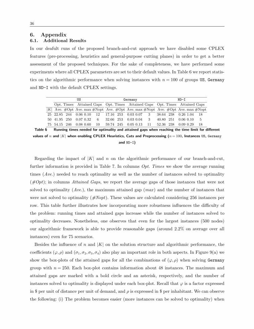
36

6. Appendix6.1. Additional Results

In our deafult runs of the proposed branch-and-cut approach we have disabled some CPLEX

features (pre-processing, heuristics and general-purpose cutting planes) in order to get a better

assessment of the proposed techniques. For the sake of completeness, we have performed some

experiments where all CPLEX parameters are set to their default values. In Table 6 we report statis-

tics on the algorithmic performance when solving instances with n = 100 of groups US, Germany

and ND-I with the default CPLEX settings.

US Germany ND-I

Opt. Times Attained Gaps Opt. Times Attained Gaps Opt. Times Attained Gaps

|K| Ave. #Opt Ave. max #Nopt Ave. #Opt Ave. max #Nopt Ave. #Opt Ave. max #Nopt

25 22.85 244 0.06 0.10 12 17.16 253 0.03 0.07 3 38.64 238 0.26 1.04 18

50 41.95 250 0.07 0.32 6 32.66 253 0.03 0.04 3 40.80 251 0.06 0.10 5

75 54.15 246 0.08 0.60 10 59.74 245 0.05 0.13 11 52.36 238 0.09 0.29 18

Table 6 Running times needed for optimality and attained gaps when reaching the time limit for different

values of n and |K| when enabling CPLEX Heuristics, Cuts and Preprocessing (n= 100, Instances US, Germany

and ND-I)

Regarding the impact of |K| and n on the algorithmic performance of our branch-and-cut,

further information is provided in Table 7. In columns Opt. Times we show the average running

times (Ave.) needed to reach optimality as well as the number of instances solved to optimality

(#Opt); in columns Attained Gaps, we report the average gaps of those instances that were not

solved to optimality (Ave.), the maximum attained gap (max ) and the number of instances that

were not solved to optimality (#Nopt). These values are calculated considering 256 instances per

row. This table further illustrates how incorporating more robustness influences the difficulty of

the problem: running times and attained gaps increase while the number of instances solved to

optimality decreases. Nonetheless, one observes that even for the largest instances (500 nodes)

our algorithmic framework is able to provide reasonable gaps (around 2.2% on average over all

instances) even for 75 scenarios.

Besides the influence of n and |K| on the solution structure and algorithmic performance, the

coefficients (ϕ,ρ) and (σ1, σ2, σ3, σ4) also play an important role in both aspects. In Figure 9(a) we

show the box-plots of the attained gaps for all the combinations of (ϕ,ρ) when solving Germany

group with n = 250. Each box-plot contains information about 48 instances. The maximum and

attained gaps are marked with a bold circle and an asterisk, respectively, and the number of

instances solved to optimality is displayed under each box-plot. Recall that ϕ is a factor expressed

in $ per unit of distance per unit of demand, and ρ is expressed in $ per inhabitant. We can observe

the following: (i) The problem becomes easier (more instances can be solved to optimality) when

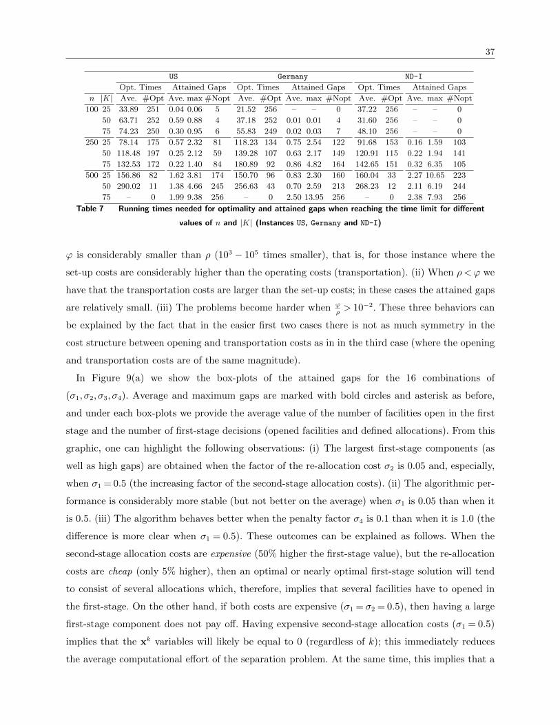
37

US Germany ND-I

Opt. Times Attained Gaps Opt. Times Attained Gaps Opt. Times Attained Gaps

n |K| Ave. #Opt Ave. max #Nopt Ave. #Opt Ave. max #Nopt Ave. #Opt Ave. max #Nopt

100 25 33.89 251 0.04 0.06 5 21.52 256 – – 0 37.22 256 – – 0

50 63.71 252 0.59 0.88 4 37.18 252 0.01 0.01 4 31.60 256 – – 0

75 74.23 250 0.30 0.95 6 55.83 249 0.02 0.03 7 48.10 256 – – 0

250 25 78.14 175 0.57 2.32 81 118.23 134 0.75 2.54 122 91.68 153 0.16 1.59 103

50 118.48 197 0.25 2.12 59 139.28 107 0.63 2.17 149 120.91 115 0.22 1.94 141

75 132.53 172 0.22 1.40 84 180.89 92 0.86 4.82 164 142.65 151 0.32 6.35 105

500 25 156.86 82 1.62 3.81 174 150.70 96 0.83 2.30 160 160.04 33 2.27 10.65 223

50 290.02 11 1.38 4.66 245 256.63 43 0.70 2.59 213 268.23 12 2.11 6.19 244

75 – 0 1.99 9.38 256 – 0 2.50 13.95 256 – 0 2.38 7.93 256

Table 7 Running times needed for optimality and attained gaps when reaching the time limit for different

values of n and |K| (Instances US, Germany and ND-I)

ϕ is considerably smaller than ρ (103 − 105 times smaller), that is, for those instance where the

set-up costs are considerably higher than the operating costs (transportation). (ii) When ρ<ϕ we

have that the transportation costs are larger than the set-up costs; in these cases the attained gaps

are relatively small. (iii) The problems become harder when ϕρ> 10−2. These three behaviors can

be explained by the fact that in the easier first two cases there is not as much symmetry in the

cost structure between opening and transportation costs as in in the third case (where the opening

and transportation costs are of the same magnitude).

In Figure 9(a) we show the box-plots of the attained gaps for the 16 combinations of

(σ1, σ2, σ3, σ4). Average and maximum gaps are marked with bold circles and asterisk as before,

and under each box-plots we provide the average value of the number of facilities open in the first

stage and the number of first-stage decisions (opened facilities and defined allocations). From this

graphic, one can highlight the following observations: (i) The largest first-stage components (as

well as high gaps) are obtained when the factor of the re-allocation cost σ2 is 0.05 and, especially,

when σ1 = 0.5 (the increasing factor of the second-stage allocation costs). (ii) The algorithmic per-

formance is considerably more stable (but not better on the average) when σ1 is 0.05 than when it

is 0.5. (iii) The algorithm behaves better when the penalty factor σ4 is 0.1 than when it is 1.0 (the

difference is more clear when σ1 = 0.5). These outcomes can be explained as follows. When the

second-stage allocation costs are expensive (50% higher the first-stage value), but the re-allocation

costs are cheap (only 5% higher), then an optimal or nearly optimal first-stage solution will tend

to consist of several allocations which, therefore, implies that several facilities have to opened in

the first-stage. On the other hand, if both costs are expensive (σ1 = σ2 = 0.5), then having a large

first-stage component does not pay off. Having expensive second-stage allocation costs (σ1 = 0.5)

implies that the xk variables will likely be equal to 0 (regardless of k); this immediately reduces

the average computational effort of the separation problem. At the same time, this implies that a

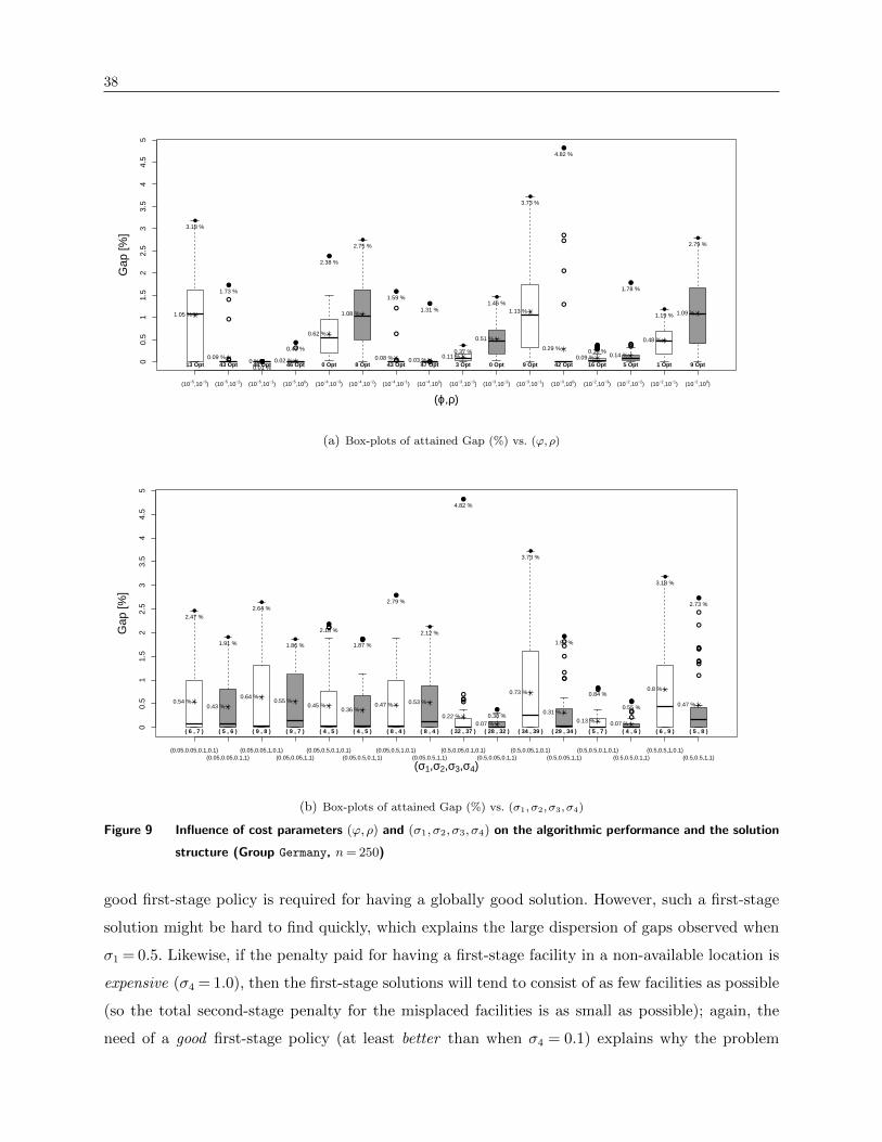
38

●

●

●

●● ●●●●

●●

●

●

●●

●

●

●

●

●

●

●

●

●●

●●●●●●●●● ●

●

●●

(ϕ,ρ)

Gap

[%]

(10−5,10−3) (10−5,10−2) (10−5,10−1) (10−5,100) (10−4,10−3) (10−4,10−2) (10−4,10−1) (10−4,100) (10−3,10−3) (10−3,10−2) (10−3,10−1) (10−3,100) (10−2,10−3) (10−2,10−2) (10−2,10−1) (10−2,100)

00.

51

1.5

22.

53

3.5

44.

55

1.05 %

●

3.18 %

13 Opt0.09 %

●

1.73 %

43 Opt 0 % ●

0.01 %48 Opt0.02 %

●

0.43 %

46 Opt

0.62 %

●

2.38 %

0 Opt

1.08 %

●

2.75 %

8 Opt0.08 %

●

1.59 %

43 Opt0.03 %

●

1.31 %

47 Opt0.11 %

●

0.37 %

3 Opt

0.51 %

●

1.46 %

0 Opt

1.13 %

●

3.73 %

9 Opt

0.29 %

●

4.82 %

42 Opt0.09 %

●

0.38 %

16 Opt

0.14 %

●

1.78 %

5 Opt

0.48 %

●

1.19 %

1 Opt

1.09 %

●

2.79 %

9 Opt

(a) Box-plots of attained Gap (%) vs. (ϕ,ρ)

●●●

●●●

●

●●

●

●●

●

●

●

●

●

●

●

●

●●●

●

●●

●

●

●

●●

●

●

●

●

●

●

●

(σ1,σ2,σ3,σ4)

Gap

[%]

(0.05,0.05,0.1,0.1) (0.05,0.05,1,0.1) (0.05,0.5,0.1,0.1) (0.05,0.5,1,0.1) (0.5,0.05,0.1,0.1) (0.5,0.05,1,0.1) (0.5,0.5,0.1,0.1) (0.5,0.5,1,0.1) (0.05,0.05,0.1,1) (0.05,0.05,1,1) (0.05,0.5,0.1,1) (0.05,0.5,1,1) (0.5,0.05,0.1,1) (0.5,0.05,1,1) (0.5,0.5,0.1,1) (0.5,0.5,1,1)

00.

51

1.5

22.

53

3.5

44.

55

0.54 %

●

2.47 %

( 6 , 7 )

0.43 %

●

1.91 %

( 5 , 6 )

0.64 %

●

2.64 %

( 9 , 8 )

0.55 %

●

1.86 %

( 9 , 7 )

0.45 %

●

2.18 %

( 4 , 5 )

0.36 %

●

1.87 %

( 4 , 5 )

0.47 %

●

2.79 %

( 8 , 4 )

0.53 %

●

2.12 %

( 8 , 4 )

0.22 %

●

4.82 %

( 32 , 37 )0.07 %

●

0.38 %

( 28 , 32 )

0.73 %

●

3.73 %

( 34 , 39 )

0.31 %

●

1.92 %

( 29 , 34 )

0.13 %

●

0.84 %

( 5 , 7 )0.07 %

●

0.55 %

( 4 , 6 )

0.8 %

●

3.18 %

( 6 , 9 )

0.47 %

●

2.73 %

( 5 , 8 )

(b) Box-plots of attained Gap (%) vs. (σ1, σ2, σ3, σ4)

Figure 9 Influence of cost parameters (ϕ,ρ) and (σ1, σ2, σ3, σ4) on the algorithmic performance and the solution

structure (Group Germany, n= 250)

good first-stage policy is required for having a globally good solution. However, such a first-stage

solution might be hard to find quickly, which explains the large dispersion of gaps observed when

σ1 = 0.5. Likewise, if the penalty paid for having a first-stage facility in a non-available location is

expensive (σ4 = 1.0), then the first-stage solutions will tend to consist of as few facilities as possible

(so the total second-stage penalty for the misplaced facilities is as small as possible); again, the

need of a good first-stage policy (at least better than when σ4 = 0.1) explains why the problem

39

becomes harder, especially when a greater value of σ1 pushes towards solutions with more facilities

opened in the first stage.

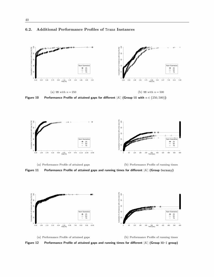
40

6.2. Additional Performance Profiles of Trans Instances

Gap [%]

Cum

ulat

ive

% o

f Ins

tanc

es w

ith G

ap (

%)

[%]

●●●●●●●●●●●●●●●●●●●●●●●●●●●●●●●●●●●●●●●●●●●●●●●●●●●●●●●●●●●●●●●●●●●●●●●●●●●●●●●●●●●●●●●●●●●●●●●●●●●●●●●●●●●●●●●●●●●●●●●●●●●●●●●●●●●●●●●●●●●●●●●●●●●●●●●●●●●●●●●●●●●●●●●●●●●●●●●●●●●●

●●●●●●●●●●●●●●●●

●●●●●●●●●●● ●●●●●●●●●● ●●●●●● ●●●●●●●●●

●●●●●●●●●●● ●●●●● ● ●●●● ● ● ●

0.00 0.23 0.46 0.70 0.93 1.16 1.39 1.63 1.86 2.09 2.32

020

4060

8010

0

●

Num Scenarios

255075

(a) US with n= 250

Gap [%]

Cum

ulat

ive

% o

f Ins

tanc

es w

ith G

ap (

%)

[%]

●●●●●●●●●●●●●●●●●●●●●●●●●●●●●●●●●●●●●●●●●●●●●●●●●●●●●●●●●●●●●●●●●●●●●●●●●●●●●●●●●●●●●●●●●●●●●●●●●●●

●●●●●●●●●●●●●●●●●●

●●●●●●●●●●●●●●●●●●●●●●●●

●●●●●●●●●●●●●

●●●●●●●●●●●●●●●●●●●●●●●●●●●●●●●●●●●●●●●●●●●●●●●●●●●●●●●●●●●●●●●●●●●

●●●●●●●●●●●●

●●●●●●●●●●●●●●●●●

● ●●●●●

0.00 0.94 1.88 2.81 3.75 4.69 5.63 6.57 7.50 8.44 9.38

020

4060

8010

0

●

Num Scenarios

255075

(b) US with n= 500

Figure 10 Performance Profile of attained gaps for different |K| (Group US with n∈ {250,500})

Gap [%]

Cum

ulat

ive

% o

f Ins

tanc

es w

ith G

ap (

%)

[%]

●●●●●●●●●●●●●●●●●●●●●●●●●●●●●●●●●●●●●●●●●●●●●●●●●●●●●●●●●●●●●●●●●●●●●●●●●●●●●●●●●●●●●●●●●●●●●●●●●●●●●●●●●●●●●●●●●●●●●●●●●●●●●●●●●●●●●●●●●●●●●●●●●●●●●●●●●●●●●●●●●●●●●●●●●●●●●●●●●●●●●●●●●●●●●●●●●●●●●●●●●●●●●●●●●●●●●●●●●●●●●●●●●●●●●●●●●●●●●●●●●●●●●●●●●●●●●●●●●●●●●●●●●●●●●●●●●●●●●●●●●●●●●●●●●●●●●●●●●●●●●●●●●●●●●●●●●●●●●●●●●●●●●●●●●●●●●●●●●●●●●●●●●●●●●●●●●●●●●●●●●●●●●●●●●●●●●●●●●●●●●●●●●●●●●●●●●●●●●●●●●●●●●●●●●●●●●●●●●●●●●●●●●●●●●●●●●●●●●●●●●●●●●●●●●●●●●●●●●●●●●●●●●●●●●●●●●●●●●●●●●●●●●●●●●●●●●●●●●●●●●●●●●●●●●●●●●●●●●●●●●●●●●●●●●●●●●●●●●●●●●●●●●●●●●●●●●●●●●●●●●●●●●●●●●●●●●●●●●●●●●●●●●●●●●●●●●●●●●●●●●●●●●●●●●●●●●●●●●●●●●●●●●●●●●●●●●●●●●●●●●●●●●●●●●●●●●●●●●●●●●●●●●●●●●●●●●●●●●●●●●●●●●●●●●●●●●●●●●●●●●●●●●●●●●●●●●●

●●●●●●●●●●●●●●●●●●●●●●●●●●●●●●●●●●

●●●●●●●●●●●●●●●●●●●●

0.00 1.39 2.79 4.18 5.58 6.97 8.37 9.76 11.16 12.55 13.95

020

4060

8010

0

●

Num Scenarios

255075

(a) Performance Profile of attained gaps

Time [sec]

Cum

ulat

ive

% o

f Ins

tanc

es w

ith a

tim

e (s

ec)

[%]

●●●●●●●●●●●●●●●●●●●●●●●●●●●●●●●●●●●●●●●●●●●●●●●●●●●●●●●●●●●●●●●●●●●●●●●●●●●●●●●●●●●●●●●●●●●●●●●●●●●●●●●●●●●●●●●●●●●●●●●●●●●●●●●●●●●●●●●●●●●●●●●●●●●●●●●●●●●●●●●●●●●●●●●●●●●●●●●●●●●●●●●●●●●●●●●●●●●●●●●●●●●●

●●●●●●●●●●●●●●●●●●●●●●●●●●●●●●●●●●

●●●●●●●●●●●●●●●●●●●●●●●●●●●●●●●●●●

●●●●●●●●●●●●●●●●●●●●●●●●●●●●●●●●●●

●●●●●●●●●●●●●●●●●●●●●●●●●●●●●●●●●●

●●●●●●●●●●●●●●●●●●●●●●●●●●●●●●●●●●

●●●●●●●●●●●●●●●●●●●●●●●●●●●●●●●●●●

●●●●●●●●●●●●●●●●●●●●●●●●●●●●●●●●●●●●●●●●●●●●●●●●●●

●●●●●●●●●●●●●●●●●●●●●●●●●● ● ● ●●●●●●●●●●●●●●●●●●●●●●●●●●●●●●●●●●●●●●●●●●●●●●●●●●●●●●●●●●●●●●●●●●●●●●●●●●●●●●●●●●●●●●●●●●●●●●●●●●●●●●●●●●●●●●●●●●●●●●●●●●●●●●●●●●●●●●●●●●●●●●●●●●●●●●●●●●●●●●●●●●●●●●●●●●●●●●●●●●●●●●●●●●●●●●●●●●●●●●●●●●●●●●●●●●●●●●●●●●●●●●●●●●●●●●●●●●●●●●●●●●●●●●●●●●●●●●●●●●●●●●●●●●●●●●●●●●●●●●●●●●

0 60 120 180 240 300 360 420 480 540 600

020

4060

8010

0

●

Num Scenarios

255075

(b) Performance Profile of running times

Figure 11 Performance Profile of attained gaps and running times for different |K| (Group Germany)

Gap [%]

Cum

ulat

ive

% o

f Ins

tanc

es w

ith G

ap (

%)

[%]

●●●●●●●●●●●●●●●●●●●●●●●●●●●●●●●●●●●●●●●●●●●●●●●●●●●●●●●●●●●●●●●●●●●●●●●●●●●●●●●●●●●●●●●●●●●●●●●●●●●●●●●●●●●●●●●●●●●●●●●●●●●●●●●●●●●●●●●●●●●●●●●●●●●●●●●●●●●●●●●●●●●●●●●●●●●●●●●●●●●●●●●●●●●●●●●●●●●●●●●●●●●●●●●●●●●●●●●●●●●●●●●●●●●●●●●●●●●●●●●●●●●●●●●●●●●●●●●●●●●●●●●●●●●●●●●●●●●●●●●●●●●●●●●●●●●●●●●●●●●●●●●●●●●●●●●●●●●●●●●●●●●●●●●●●●●●●●●●●●●●●●●●●●●●●●●●●●●●●●●●●●●●●●●●●●●●●●●●●●●●●●●●●●●●●●●●●●●●●●●●●●●●●●●●●●●●●●●●●●●●●●●●●●●●●●●●●●●●●●●●●●●●●●●●●●●●●●●●●●●●●●●●●●●●●●●●●●●●●●●●●●●●●●●●●●●●●●●●●●●●●●●●●●●●●●●●●●●●●●●●●●●●●●●●●●●●●●●●●●●●●●●●●●●●●●●●●●●●●●●●●

●●●●●●●●●●●●●●●●●●●●●●●●●●●●●●●●●●

●●●●●●●●●●●●●●●●●●●●●●●●●●●●●●●●●●●●

●●●●●●●●●●●●●●●●●●●●●●●●●●●●●●●●●●

●●●●●●●●●●●●●●●●●●●●●●●●●●●●●●●●●●

●●●●●●●●●●●●●●●●●●●●●●●●●●●●●●●●●●●●●●●●●●●●●●●

●●●●●●●● ●●●●●● ●●●● ●●●●

0.00 1.06 2.13 3.19 4.26 5.32 6.39 7.45 8.52 9.58 10.65

020

4060

8010

0

●

Num Scenarios

255075

(a) Performance Profile of attained gaps

Time [sec]

Cum

ulat

ive

% o

f Ins

tanc

es w

ith a

tim

e (s

ec)

[%]

●●●●●●●●●●●●●●●●●●●●●●●●●●●●●●●●●●●●●●●●●●●●●●●●●●●●●●●●●●●●●●●●●●●●●●●●●●●●●●●●●●●●●●●●●●●●●●●●●●●●●●●●●●●●●●●●●●●●●●●●●●●●●●●●●●●●●●●●●●●●●●●●●●●●●●●●●●●●●●●●●●●●●●●●●●●●●●●●●●●●●●●●●●●●●●●●●●●●●●●●●●●●●●●●●●●●●●●●●●●●●●●●●●●●●●●●●●●●●●●●●●●●●●●●●●●●●●●●●●●●●●●●●●●●●●●●●●●●●●●●●●●●●●●●●●●●●●●●●●●●●●●●●●●●●●●●●●●●●●●●●●●

●●●●●●●●●●●●●●●●●●●●●●●●●●●●●●●●●●

●●●●●●●●●●●●●●●●●●●●●●●●●●●●●●●●●●●●●●●●●●●●●●●●●●●

●●●●●●●●●●●●●●●●●●●●●●●●●●●●●●● ●● ● ●●●●●●●●●●●●●●●●●●●●●●●●●●●●●●●●●●●●●●●●●●●●●●●●●●●●●●●●●●●●●●●●●●●●●●●●●●●●●●●●●●●●●●●●●●●●●●●●●●●●●●●●●●●●●●●●●●●●●●●●●●●●●●●●●●●●●●●●●●●●●●●●●●●●●●●●●●●●●●●●●●●●●●●●●●●●●●●●●●●●●●●●●●●●●●●●●●●●●●●●●●●●●●●●●●●●●●●●●●●●●●●●●●●●●●●●●●●●●●●●●●●●●●●●●●●●●●●●●●●●●●●●●●●●●●●●●●●●●●●●●●●●●●●●●●●●●●●●●●●●●●●●●●●●●●●●●●●●●●●●●●●●●●

0 60 120 180 240 300 360 420 480 540 600

020

4060

8010

0

●

Num Scenarios

255075

(b) Performance Profile of running times

Figure 12 Performance Profile of attained gaps and running times for different |K| (Group ND-I group)

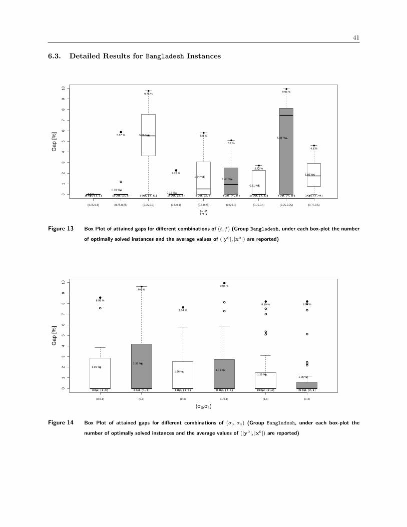
41

6.3. Detailed Results for Bangladesh Instances

●

●

●

(t,f)

Gap

[%]

(0.25,0.1) (0.25,0.25) (0.25,0.5) (0.5,0.1) (0.5,0.25) (0.5,0.5) (0.75,0.1) (0.75,0.25) (0.75,0.5)

01

23

45

67

89

10

0 %18 Opt, ( 1 , 1 )

0.39 %

●

5.87 %

16 Opt, ( 2 , 3 )

5.56 %

●

9.75 %

1 Opt, ( 3 , 11 )0.13 %

●

2.26 %

17 Opt, ( 2 , 9 )

1.64 %

●

5.8 %

9 Opt, ( 2 , 6 )

1.43 %

●

5.1 %

5 Opt, ( 4 , 27 )

0.81 %

●

2.72 %

12 Opt, ( 3 , 12 )

5.31 %

●

9.94 %

6 Opt, ( 4 , 15 )

1.85 %

●

4.6 %

1 Opt, ( 7 , 40 )

Figure 13 Box Plot of attained gaps for different combinations of (t, f) (Group Bangladesh, under each box-plot the number

of optimally solved instances and the average values of (|y0|, |x0|) are reported)

●

●

●

●

●

●

●

●

●

●

●

●

●

●

●

●

●

●

(σ3,σ4)

Gap

[%]

(0,0.1) (0,1) (0,4) (1,0.1) (1,1) (1,4)

01

23

45

67

89

10

1.99 %

●

8.56 %

8 Opt, ( 2 , 3 )

2.32 %

●

9.6 %

8 Opt, ( 1 , 3 )

1.56 %

●

7.64 %

8 Opt, ( 1 , 3 )

1.71 %

●

9.94 %

21 Opt, ( 2 , 4 )

1.29 %

●

8.19 %

23 Opt, ( 2 , 4 )

1.05 %

●

8.19 %

26 Opt, ( 2 , 6 )

Figure 14 Box Plot of attained gaps for different combinations of (σ3, σ4) (Group Bangladesh, under each box-plot the

number of optimally solved instances and the average values of (|y0|, |x0|) are reported)

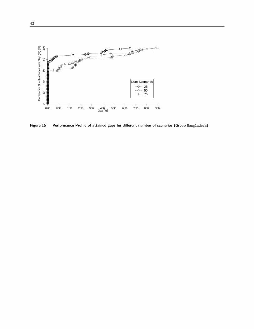
42

Gap [%]

Cum

ulat

ive

% o

f Ins

tanc

es w

ith G

ap (

%)

[%]

●●●●●●●●●●●●●●●●●●●●●●●●●●●●●●●●●●●●●●●●●●●●●●●●●●●●●●

●●●●●

●●●● ● ● ●●

●●● ● ●

0.00 0.99 1.99 2.98 3.97 4.97 5.96 6.96 7.95 8.94 9.94

020

4060

8010

0

●

Num Scenarios

255075

Figure 15 Performance Profile of attained gaps for different number of scenarios (Group Bangladesh)

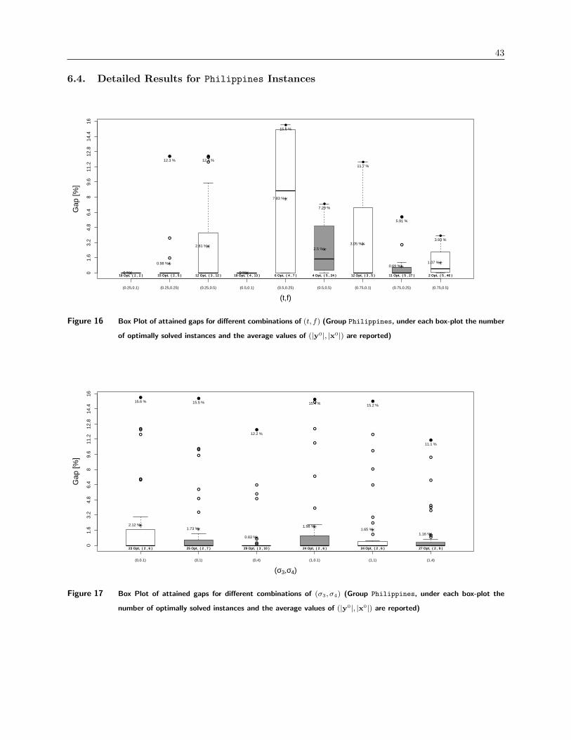
43

6.4. Detailed Results for Philippines Instances

●

●

●

●●

●

●

●

(t,f)

Gap

[%]

(0.25,0.1) (0.25,0.25) (0.25,0.5) (0.5,0.1) (0.5,0.25) (0.5,0.5) (0.75,0.1) (0.75,0.25) (0.75,0.5)

01.

63.

24.

86.

48

9.6

11.2

12.8

14.4

16

0 %18 Opt, ( 2 , 2 )

0.98 %

●

12.3 %

15 Opt, ( 2 , 5 )

2.81 %

●

12.3 %

12 Opt, ( 3 , 12 )0 %

18 Opt, ( 4 , 13 )

7.83 %

●

15.6 %

6 Opt, ( 4 , 7 )

2.5 %

●

7.29 %

4 Opt, ( 5 , 24 )

3.05 %

●

11.7 %

12 Opt, ( 3 , 5 )

0.69 %

●

5.91 %

11 Opt, ( 5 , 27 )

1.07 %

●

3.93 %

2 Opt, ( 5 , 46 )

Figure 16 Box Plot of attained gaps for different combinations of (t, f) (Group Philippines, under each box-plot the number

of optimally solved instances and the average values of (|y0|, |x0|) are reported)

●

●●

●

●

●

●

●

●

●

●

●

●

●

●

●

●

●

●

●

●

●

●

●

●

●

●

●

●

●

●

●

●

●

●

●

●

●

●

●

●

●

(σ3,σ4)

Gap

[%]

(0,0.1) (0,1) (0,4) (1,0.1) (1,1) (1,4)

01.

63.

24.

86.

48

9.6

11.2

12.8

14.4

16

2.12 %

●

15.6 %

23 Opt, ( 2 , 6 )

1.73 %

●

15.5 %

25 Opt, ( 2 , 7 )

0.83 %

●

12.2 %

29 Opt, ( 3 , 10 )

1.98 %

●

15.4 %

24 Opt, ( 2 , 6 )

1.65 %

●

15.2 %

24 Opt, ( 2 , 6 )

1.16 %

●

11.1 %

27 Opt, ( 2 , 9 )

Figure 17 Box Plot of attained gaps for different combinations of (σ3, σ4) (Group Philippines, under each box-plot the

number of optimally solved instances and the average values of (|y0|, |x0|) are reported)

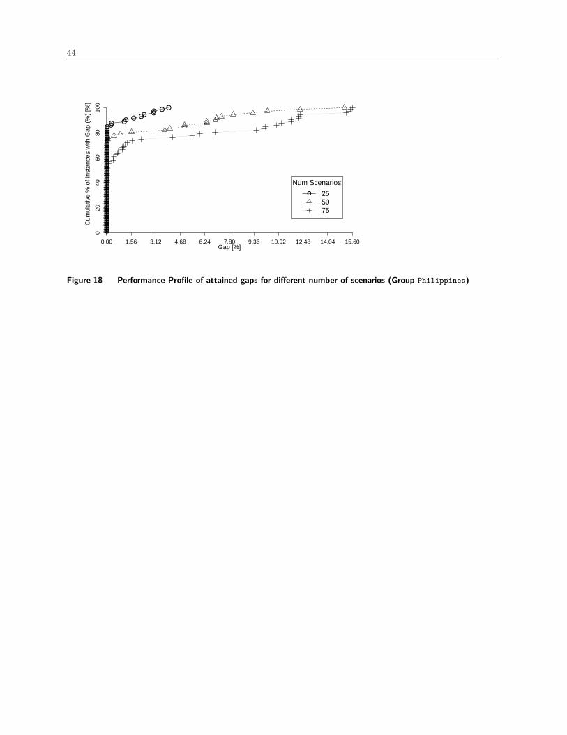
44

Gap [%]

Cum

ulat

ive

% o

f Ins

tanc

es w

ith G

ap (

%)

[%]

●●●●●●●●●●●●●●●●●●●●●●●●●●●●●●●●●●●●●●●●●●●●●●●●●●●●●●●●●●●●●●●

●●● ●● ●●

● ●

0.00 1.56 3.12 4.68 6.24 7.80 9.36 10.92 12.48 14.04 15.60

020

4060

8010

0

●

Num Scenarios

255075

Figure 18 Performance Profile of attained gaps for different number of scenarios (Group Philippines)

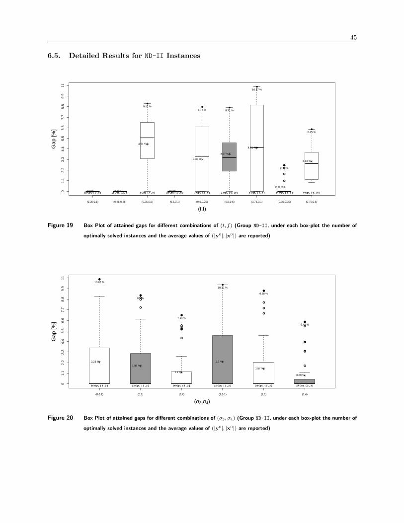
45

6.5. Detailed Results for ND-II Instances

●

●

●

●

(t,f)

Gap

[%]

(0.25,0.1) (0.25,0.25) (0.25,0.5) (0.5,0.1) (0.5,0.25) (0.5,0.5) (0.75,0.1) (0.75,0.25) (0.75,0.5)

01.

12.

23.

34.

45.

56.

67.

78.

89.

911

0 %18 Opt, ( 0 , 0 )

0 %18 Opt, ( 2 , 3 )

4.91 %

●

9.12 %

3 Opt, ( 4 , 8 )0 %

18 Opt, ( 3 , 5 )

3.33 %

●

8.77 %

7 Opt, ( 3 , 5 )

3.87 %

●

8.71 %

1 Opt, ( 6 , 18 )

4.51 %

●

10.87 %

8 Opt, ( 3 , 4 )

0.45 %

●

2.71 %

14 Opt, ( 3 , 6 )

3.13 %

●

6.45 %

0 Opt, ( 8 , 36 )

Figure 19 Box Plot of attained gaps for different combinations of (t, f) (Group ND-II, under each box-plot the number of

optimally solved instances and the average values of (|y0|, |x0|) are reported)

●

●

●

●●

●

●

●●●

●

●

●

●

●

●

●

●

●●

●

●

(σ3,σ4)

Gap

[%]

(0,0.1) (0,1) (0,4) (1,0.1) (1,1) (1,4)

01.

12.

23.

34.

45.

56.

67.

78.

89.

911

2.28 %

●

10.87 %

20 Opt, ( 2 , 2 )

1.86 %

●

9.2 %

23 Opt, ( 2 , 2 )

1.2 %

●

7.14 %

26 Opt, ( 1 , 2 )

2.3 %

●

10.31 %

21 Opt, ( 2 , 2 )

1.57 %

●

9.68 %

24 Opt, ( 2 , 3 )

0.89 %

●

6.45 %

27 Opt, ( 2 , 3 )

Figure 20 Box Plot of attained gaps for different combinations of (σ3, σ4) (Group ND-II, under each box-plot the number of

optimally solved instances and the average values of (|y0|, |x0|) are reported)

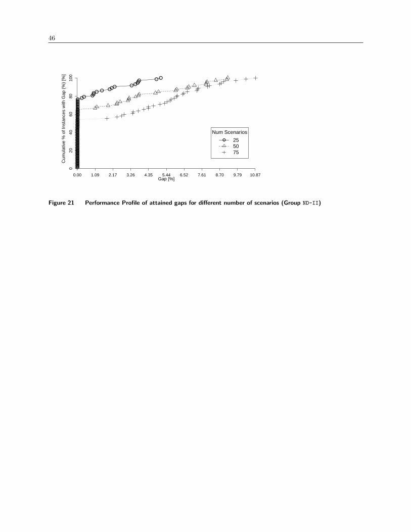
46

Gap [%]

Cum

ulat

ive

% o

f Ins

tanc

es w

ith G

ap (

%)

[%]

●●●●●●●●●●●●●●●●●●●●●●●●●●●●●●●●●●●●●●●●●●●●●●●●●●●●●●● ●● ●●

●● ● ●●● ●●●●● ● ●

0.00 1.09 2.17 3.26 4.35 5.44 6.52 7.61 8.70 9.79 10.87

020

4060

8010

0

●

Num Scenarios

255075

Figure 21 Performance Profile of attained gaps for different number of scenarios (Group ND-II)