The Redistributional Impact of Nonlinear Electricity Pricingfaculty.haas.berkeley.edu/borenste/download/AEJEP12NonlinearElec.pdfusing estimates of price and income elasticity of demand

56

American Economic Journal: Economic Policy 2012, 4(3): 56–90 http://dx.doi.org/10.1257/pol.4.3.56

With rising energy costs and growing awareness of the threat of climate change, policy makers are increasingly coming to the realization that retail energy

prices are going to have to rise in order to reflect the full cost of consumption. At the same time, there is concern that higher energy prices—whether attributable to green-house gas policies, resource scarcity, or market power of sellers—will dispropor-tionately impact the poor. In the electric utility sector, this tension between income distribution concerns and high energy prices has been recognized for decades. In the 1970s and 1980s these concerns led to widespread adoption of increasing-block pricing (IBP) of electricity—also commonly called inverted-block pricing, increasing-tier pricing, or lifeline rates (though some lifeline rates are means tested). IBP increases the marginal price charged per unit of consumption as the customer consumes more units during a billing period. Supporters of IBP argue that these tariffs promote conservation by setting high marginal prices for many consumers while protecting small energy consumers—who are presumed to be poorer on aver-age—by keeping the price for a baseline level of consumption relatively low.1

1 Declining-block pricing—under which the marginal price of electricity to the customer is lower for units of consumption beyond a certain baseline level—had been common in the 1960s and 1970s. In the following decades, with increasing focus on conservation, it became seen as promoting wasteful consumption of power, despite the fact that a two-part tariff almost surely is a closer reflection than IBP of the true cost of serving a residential customer.

The Redistributional Impact of Nonlinear Electricity Pricing†

By Severin Borenstein*

Electricity regulators often mandate increasing-block pricing (IBP)—i.e., marginal price increases with the customer’s average daily usage—to protect low-income households from rising costs. IBP has no cost basis, raising a classic conflict between efficiency and distributional goals. Combining household-level utility billing data with census data on income, I find that IBP in California results in modest wealth redistribution, but creates substantial deadweight loss relative to the transfers. I also show that a common approach to studying income distribution effects by using median household income within census block groups may be misleading. (JEL D31, L11, L51, L94, L98, Q41, Q48)

* Haas School of Business, University of California, Berkeley, CA 94720-1900 (e-mail: [email protected]). I am grateful to Koichiro Ito for excellent research assistance and very helpful comments, and to Andrew Bell, Jim Bushnell, David Card, Raj Chetty, Howard Chong, Lucas Davis, Stephen Holland, Patrick Kline, Chris Knittel, Bill Marcus, Erich Muehlegger, Karen Notsund, Nancy Ryan, Emmanuel Saez, Glen Weyl, Frank Wolak, an anonymous referee, participants in the 2008 POWER Conference, the winter 2010 NBER Industrial Organization program meeting, and seminar audiences at UC Berkeley, Columbia, MIT, New York University, and UC San Diego for very helpful comments and discussions.

† To comment on this article in the online discussion forum, or to view additional materials, visit the article page at http://dx.doi.org/10.1257/pol.4.3.56.

ContentsThe Redistributional Impact of Nonlinear Electricity Pricing† 56

I. Previous Studies of the Distributional Impacts of Electricity Pricing 58II. Increasing-Block Residential Electricity Rates in California 59III. Data Sources 62IV. Creating Benchmark and Counterfactual Bills 65V. Matching Households to Income Brackets 66VI. Refining the Redistribution Estimates 71VII. Demand Elasticity and the Efficiency Costs of Income Redistribution 76VIII. Increasing-Block Pricing versus a Tariff for Low-Income Households 81IX. Conclusion 84Appendix: Utilization of CARE Participation Information in Ranking Methods 86References 88

http://dx.doi.org/10.1257/pol.4.3.56

VoL. 4 No. 3 57BorENstEIN: rEdIstrIButIoNAL ImPACt of ELECtrICIty PrICINg

California’s regulated utilities adopted increasing-block residential electricity tar-iffs in the 1980s. Prior to the California electricity crisis in 2000–2001, all three of the large regulated electric utilities in California—Pacific Gas and Electric (PG&E), Southern California Edison (SCE), and San Diego Gas and Electric (SDG&E)—had two-tiered residential rate structures where the marginal price in the second tier was 15 percent–18 percent higher than in the first tier. That was in line with the structure in many other states. One recent survey of 61 US utilities (BC Hydro 2008), found that about one-third of them use IBP for residential customers. Many more utilities and regulators are currently considering adopting IBP tariffs.

After the California electricity crisis, these three investor-owned utilities (IOUs) needed to raise substantial revenues, but regulators and state legislators were con-cerned about the impact on lower-income households. Regulators adopted a five-tier increasing-block retail pricing structure where the prices on the first two tiers were virtually frozen at pre-crisis levels and incremental revenue needs were to be col-lected by raising prices on tiers 3, 4, and 5. The result has been a much more extreme increasing-block tariff structure. By 2008, the price on the highest block—which is the marginal price for about 6 to 9 percent of all residential customers—ranged from about 80 percent higher to more than triple the price on the lowest block, depending on the utility.

Regardless of one’s views of the externality costs of electricity consumption and the need for conservation, it is clear that increasing-block electricity pricing dis-torts the relative marginal prices that different customers face.2 Thus, the use of increasing-block pricing presents a classic tradeoff between efficiency and distribu-tional effects in regulated tariff design. There is, however, very little firm evidence on the magnitude of this tradeoff, and none that is based on a large-scale systematic empirical study.

Combining residential bill data with income data at the census block group level, I first develop an approach that yields bounds on the income redistribution effects of these IBP tariffs. This approach and the resulting bounds are related to the lit-erature on ecological regression.3 I then develop an estimate of redistribution based on those bounds that uses additional information to more accurately estimate the income status of individual customers. I find that low-income customers benefit from California’s current steeply tiered rate structure compared to the bills they would have paid under a flat rate tariff. If this were the only electricity program aimed at helping the poor, I find that IBP would lower the bills of SCE customers in the lowest income bracket (approximately a quintile) by about $11 per month, with somewhat smaller changes for the other two utilities.

Such analysis of transfers raises the question of the cost in terms of inefficient pricing. Under a wide range of demand elasticity assumptions, I calculate the

2 Some have argued that heavy residential users impose higher costs per unit consumption. Such suggestions are based on the correlation between the timing of consumption patterns and overall use, but the increasing-block tariff takes no account of the timing of use so the connection is quite indirect. See Marcus and Ruszovan (2007). Borenstein (2011) presents data analysis for PG&E customers that suggests high-use customers are on average slightly more costly to serve due to the timing of their demand, but the differential is a tiny fraction of the price spread between lower and higher blocks of the IBP tariffs that I analyze.

3 See Goodman (1953), Freedman (2001), and Wakefield (2004).

58 AmErICAN ECoNomIC JourNAL: ECoNomIC PoLICy August 2012

deadweight loss that would result from IBP. For all of the plausible long-run elas-ticity scenarios, it seems very likely that the efficiency costs of IBP would be sub-stantial compared to the redistributional impact. An interesting exception arises if the marginal cost of electricity were quite high (on the order of three times higher than wholesale electricity prices during the sample period), in which case the IBP tariffs that I study for California could actually reduce deadweight loss compared to a break-even flat-rate tariff.

Increasing-block rates are not, however, the only program targeted at helping low-income customers with electricity costs. Electric utilities in California, as in many other states, have a low-income energy assistance program that offers lower rates to customers who meet some means test. I examine that program as well, called the CARE program in California. I find that a means-tested program that gives a lower flat rate to low-income households than to others is likely to create less deadweight loss per dollar transfered to the poor. I also find that the presence of the CARE program reduces the redistributional effect of IBP by more than half.

Separate from the analysis of electricity rates, the approach I propose for analyz-ing redistributional effects has implications for a wide variety of studies that use census block group level data to look at the effect of business or public policies on income distribution or vice versa. Many studies use the median household income for a census block group to represent the income of all households in that area. I show, however, that there is very large heterogeneity of household incomes within census block groups and that the use of median household income greatly truncates the income distribution. Thus, studying publicly available data on income distribu-tion both across and within census block groups could be very informative, particu-larly for analyzing impacts on low-income households.

I. Previous Studies of the Distributional Impacts of Electricity Pricing

An active literature on IBP in the United States existed in the late 1970s and 1980s. A precursor is Feldstein (1972), who develops a model of the optimal trade-off between a fixed and volumetric charge to recover utility costs when the regulator cares about both efficiency and equity. He then applies the model to Massachusetts using estimates of price and income elasticity of demand from another study. A number of later papers attempt to infer income transfers from simulations using their own or others’ estimates of the income elasticity of demand. A few others combine billing data with household surveys of relatively small populations to infer the impact of IBP. Hennessy (1984) surveys this literature. Faruqui (2008) presents a recent analysis using the simulation approach, as well as a discussion of IBP poli-cies among US utilities.4

4 Numerous studies outside the United States are concerned with the impact of nonlinear electricity prices on the poor. Wodon, Ajwad, and Siaens (2003), and Al-Qudsi and Shatti (1987) present policy analyses of IBP in Honduras and Kuwait, respectively. Gibson and Price (1986) examine the distributional impact of two-part tariffs in the UK natural gas and electricity markets. Hancock and Price (1995) and Price and Hancock (1998) consider the distributional effects of market liberalization in the UK gas, telecom and electricity markets, including changes in the fixed and variable-rate components of the tariffs.


Inferring redistribution from estimates of income elasticity presents two prob-lems. The first is that those estimates vary widely (with large standard errors) among refereed publications, implying huge variations in the redistribution effect of IBP. The income elasticities of residential demand reported in Taylor’s (1975) survey of electricity demand estimation vary by nearly an order of magnitude, and other studies come to even more divergent estimates. The second problem is interpreta-tion of the income elasticity estimates. The standard income elasticity estimate is an attempt to capture the causal partial derivative of electricity consumption with respect to income. To the extent that the regression controls for other factors, the parameter estimated on income does not capture indirect income effects that come about from house size, number of people living in the dwelling, propensity to heat with electricity, and other factors. Nor does it capture factors that may have no causal link with low income, but are highly correlated with income and influence electricity use, such as weather. If the goal is to redistribute income to the poor through IBP, then the cross-sectional co-variation of income and usage is of interest, not the causal impact of income (directly or indirectly) on usage.

The survey-based studies tend to capture this relationship more effectively than the regression/simulation studies, but the survey studies are based on much smaller samples than I am able to use in this case. In addition, while the surveys have indi-vidual household demographics, they suffer from lower response rates and greater selection issues than data from the census. The cost of using the census data is that questions are not as targeted and the data are not available at the household level for matching to electricity billing data.

II. Increasing-Block Residential Electricity Rates in California

The analysis in this study has been carried out for all three of the large reg-ulated public utilities in California—Pacific Gas and Electric (PG&E), Southern California Edison (SCE), and San Diego Gas and Electric (SDG&E)—with fairly similar results. I focus in the body of the paper on SCE, but present the results for the other two utilities as well in the online Appendix. The conclusions are consistent across the three utilities.

The standard residential tariff for SCE during 2006 is illustrated in Figure 1. The increasing-block tariff structure implies an increasing marginal price for electricity. A SCE customer whose consumption level puts him or her on the highest tier, for instance, still pays the lower-tier rates for consumption up to 200 percent of baseline.5

The marginal rate that a residential customer pays increases as consumption increases relative to a “baseline” consumption level, as shown on the horizontal axis of Figure 1. A household’s baseline allocation is supposed to correspond to a minimal basic electricity usage. The baseline, however, is the same for all residential

5 For example, under the standard residential rate illustrated in Figure 1, a SCE customer with a baseline consumption allocation of 300 kWh during a given billing period who actually consumes 1,100 kWh would pay 11.62 cents for each of the first 300 kWh, 13.61 cents for each of the next 90 kWh, 22.01 cents for each of the next 210 kWh, 30.49 cents for each of the next 300 kWh, and 30.49 cents for each of the last 200 kWh. During 2006, the regulated prices on the fourth and fifth tier were equal, though that has not always been the case in earlier or succeeding years.


customers in a region regardless of the size of the residence or the number of people who live there. Within the region, a studio apartment receives the same baseline allocation as a four-bedroom house.6

Baseline allocations do differ by geographic regions within the utility area: SCE’s service territory is divided into six different baseline regions. This is argued to reflect variation in basic electricity need due to climate differences, but in prac-tice baselines are set based on different average usage across regions. As a result, variation is driven not only by climate differences, but also by wealth levels, average residence size, and choices to install air-conditioning. Within each climate region, the household baselines also differ between winter and summer periods, generally much higher during the summer in areas that use a lot of air conditioning. This effec-tively lowers the marginal price to many customers at the times when the wholesale cost of power is highest. In my analysis, I take the baseline allocations as fixed for IBP. Adjustments to baselines, given the existence of IBP, would obviously has redistributional impact as well. In this study I focus on comparing the existing IBP rates and baselines with a flat-rate pricing schedule.7

Prior to the California electricity crisis in 2000–2001, SCE had a two-tier rate struc-ture with prices near those on the first two tiers of the structure shown in Figure 1.

6 The baseline allocation is higher for approximately 10 percent of customers who have electric heating systems and some other electrical appliances.

7 The higher baselines in the summer approximately offset the higher summer consumption (by design), so the average rate is about the same in winter and summer. Thus, designing a separate flat rate for winter and summer that is revenue-neutral within each time period would change the results very little.

Figure 1. SCE’s Standard Retail Electricity Tariff in 2006

$0.00

$0.05

$0.10

$0.15

$0.20

$0.25

$0.30

$0.35M

argi

nal p

rice

per

kilo

wat

t-ho

ur

Consumption as a percentage of baseline quantity

100%

200%

300%

400%


All consumption above the baseline level was charged at the second-tier rate. After the extreme financial losses associated with the electricity crisis, the structure was changed to five tiers and rates were raised substantially for the third, fourth, and fifth tiers. As a result, in 2006 the marginal price on the fourth and fifth tier was nearly three times higher than on the first tier. The same qualitative changes occurred at the other two regulated utilities in California, but the resulting rates are noticably different—more steeply tiered at PG&E, less so at SDG&E—owing in part to the differences in economic losses they incurred during the California electricity crisis.

Not all residential customers of the IOUs are on the standard tariff. The largest exception from the standard tariff is customers who are on the CARE (California Alternate Rates for Energy) program, which is an income-based program that offers lower rates to low-income customers.8 At SCE, 25.2 percent of residential custom-ers were on the CARE program in 2006. The CARE program is advertised as offer-ing “a 20 percent discount” off the standard residential rates, but not all components of the bill are included in the discount, some components are not charged to CARE customers, and the exact implementation is quite complex. In practice, the discount is at least 20 percent and was up to 44 percent on marginal consumption at higher tiers during 2006. Overall, because of the discount on each tier and the fact that CARE customers consumed a higher proportion of their power on lower tiers, the average price paid per kilowatt-hour was 39 percent lower for CARE customers than for customers on the standard residential rate.

A small number of customers are on special tariffs that incorporate time-of-use elec-tricity pricing, interruptible air-conditioning use, mobilehome/RV/marina accounts, or other idiosyncratic rate structures. In aggregate, these nonstandard tariffs covered 1.4 percent of SCE’s residential customers in 2006, who consumed 2.1 percent of residential power. Most of these customers still face a five-tier tariff, but with different baseline allocations and in some cases somewhat different rates on the tiers.

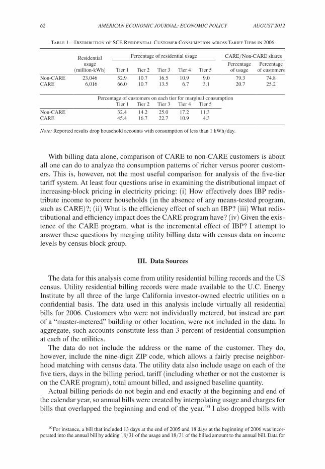
Regardless of the tariff that a customer is on, the customer has a baseline alloca-tion and his or her monthly consumption can be allocated across the five tiers of the tariff. The top panel of Table 1 shows the total quantity of residential consumption that was billed on each of the tiers during 2006. The lower-income customers who are on the CARE program consume less on average than other residential custom-ers, but there is substantial overlap in the distributions with many low-consuming customers who are not on CARE, and some CARE customers with consumption levels even out to the fifth tier. The bottom panel of Table 1 shows the proportion of households whose average daily consumption puts them on each of the five tiers in the rate structure.9 Among SCE’s non-CARE customers, for instance, 32.4 percent consume less than the baseline and therefore face the tier 1 price for their marginal consumption, while 11.3 percent consume more than 300 percent of baseline so face the tier 5 price for their marginal consumption.

8 For 2006, a residence with one or two occupants had to have a household income no higher than $28,600 in order to qualify for CARE, with the threshold increasing by $5,000 for a third occupant, and by $6,900 for each additional occupant.

9 To be precise, the bottom panel of Table 1 shows the customer-days weighted-average proportion of bills dur-ing 2006 for which marginal consumption was billed at each tier.


With billing data alone, comparison of CARE to non-CARE customers is about all one can do to analyze the consumption patterns of richer versus poorer custom-ers. This is, however, not the most useful comparison for analysis of the five-tier tariff system. At least four questions arise in examining the distributional impact of increasing-block pricing in electricity pricing: (i) How effectively does IBP redis-tribute income to poorer households (in the absence of any means-tested program, such as CARE)?; (ii) What is the efficiency effect of such an IBP? (iii) What redis-tributional and efficiency impact does the CARE program have? (iv) Given the exis-tence of the CARE program, what is the incremental effect of IBP? I attempt to answer these questions by merging utility billing data with census data on income levels by census block group.

III. Data Sources

The data for this analysis come from utility residential billing records and the US census. Utility residential billing records were made available to the U.C. Energy Institute by all three of the large California investor-owned electric utilities on a confidential basis. The data used in this analysis include virtually all residential bills for 2006. Customers who were not individually metered, but instead are part of a “master-metered” building or other location, were not included in the data. In aggregate, such accounts constitute less than 3 percent of residential consumption at each of the utilities.

The data do not include the address or the name of the customer. They do, however, include the nine-digit ZIP code, which allows a fairly precise neighbor-hood matching with census data. The utility data also include usage on each of the five tiers, days in the billing period, tariff (including whether or not the customer is on the CARE program), total amount billed, and assigned baseline quantity.

Actual billing periods do not begin and end exactly at the beginning and end of the calendar year, so annual bills were created by interpolating usage and charges for bills that overlapped the beginning and end of the year.10 I also dropped bills with

10 For instance, a bill that included 13 days at the end of 2005 and 18 days at the beginning of 2006 was incor-porated into the annual bill by adding 18/31 of the usage and 18/31 of the billed amount to the annual bill. Data for

Table 1—Distribution of SCE Residential Customer Consumption across Tariff Tiers in 2006

Residentialusage

(million-kWh)

Percentage of residential usage CARE/Non-CARE shares

Percentage PercentageTier 1 Tier 2 Tier 3 Tier 4 Tier 5 of usage of customers

Non-CARE 23,046 52.9 10.7 16.5 10.9 9.0 79.3 74.8CARE 6,016 66.0 10.7 13.5 6.7 3.1 20.7 25.2

Percentage of customers on each tier for marginal consumptionTier 1 Tier 2 Tier 3 Tier 4 Tier 5

Non-CARE 32.4 14.2 25.0 17.2 11.3CARE 45.4 16.7 22.7 10.9 4.3

Note: Reported results drop household accounts with consumption of less than 1 kWh/day.


consumption of less than 1 kWh/day. A refrigerator typically uses 1–2 kWh/day,11 so it is implausible that an occupied primary residence would fall below 1 kWh/day. Dropping these observations should permit a closer match to the census data. Including these observations does not change the qualitative results, but it increases the number of customer-days by about 1.4 percent.

Summary household income data are available from the US Census Bureau at the level of census block group (CBG), a geographic designation that on average includes about 600 households in California.12 Census block groups are consider-ably larger than the areas associated with nine-digit ZIP codes. Each nine-digit ZIP code is assigned to the CBG in which it was located.13 The analysis presented here was then carried out at the CBG level. Results presented here use 2000 census data updated to 2007 by Geolytics, but the results are very similar if the analysis is based on the original 2000 data.14

Census measures of Household Income.—Household income data at the CBG level includes median household income and mean per capita income.15 In eco-nomics, epidemiology, and other areas of research, these summary measures are frequently used by associating them with every household in the CBG.16

Unfortunately for such applications, there is considerable income heterogeneity within CBGs. This is evident from additional data released by the Census that break down households into very small income brackets for each CBG in the 2000 cen-sus. Because many brackets have zero households in many CBGs and because this is a 17 percent sample, not a census, I aggregate the data to 5 income brackets that are approximate quintile breaks: $0–$20,000; $20,000–$40,000; $40,000–$60,000; $60,000–$100,000; and over $100,000. In the 17,768 census block groups I consider in California—those served by the three investor-owned utilities—the breakpoints between these categories correspond to the 18th, 41st, 59th, and 82nd percentiles in the distribution of household income.

There would be little concern about within-CBG income heterogeneity if all of the population in a given CBG fell into one of these income brackets, but that is far

PG&E, unfortunately, did not extend beyond the end of 2006, so billing periods that ended after December 31, 2006 would be lost if I were to apply this procedure to PG&E. To greatly reduce this problem, the period of analysis for PG&E was shifted by one month and I instead studied December 2005–November 2006.

11 See http://www.energystar.gov/index.cfm?fuseaction=refrig.display_products_html.12 These are public data from the Census Summary File 3. The US Census Bureau does not suppress data when

the counts in an income category are small, but they report that some random error is added to figures to prevent exact identification in cases of small numbers.

13 About 2.8 percent of customer records did not include a nine-digit ZIP code, or did not match to a nine-digit ZIP code in the census data. In the case of nine-digit ZIP codes that did not match to the census data, I used the numerically closest nine-digit ZIP code. In the case of having only a five-digit ZIP code, those customers were allocated probabilistically among all of the nine-digit ZIP codes within the five-digit ZIP code based on the share of households that were in each of the nine-digit ZIP codes. These two approaches assigned nine-digit ZIP codes to all but 0.17 percent of the households. The remaining households were dropped.

14 For details of the updating see, http://www.geolytics.com.15 Household income data from the US Census Bureau are based on the “long form” questionnaire that is dis-

tributed to about 1/6 of all households.16 Examples in economics include hedonic real estate demand models, Bajari and Kahn (2008); auto demand,

Busse, Silva-Risso, and Zettelemeyer (2006); education valuation, Jacob and Lefgren (2007), and Hastings, Kane, and Staiger (2005); local pollution impacts on housing, Gayer, Hamilton, and Viscusi (2000); and effects of low income housing tax credits, Baum-Snow and Marion (2009). Of course, the importance of this simplification will differ depending on the empirical application.


from the case. Looking at the shares of households in each bracket, one can calcu-late a Herfindahl index to measure concentration of households within the income brackets for a given CBG. This index is the sum of the squared shares of population in each bracket. With five income groups, it has a minimum of 0.2 (if households within a CBG were evenly divided across the five brackets) and a maximum of 1 (if households were all in the same bracket). Calculating this index for the census block groups I examine in California, the average value is 0.29, indicating more dispersion than if the population within each CBG were evenly divided across any three income brackets (which would yield a value of 0.33).

Because of this within-CBG dispersion, assigning to every household within a CBG the median household income or mean per capita income for that CBG sub-stantially understates the variance in the distribution at the household level. More extreme high and low income levels are underrepresented. Figure 2 illustrates this effect for CBGs I use in California by showing the distribution of median household incomes within CBGs and the assignment of individual households to each of the five income brackets. The median household income data are weighted by house-holds across CBGs, so Figure 2 shows that while about 18 percent of households report income below $20,000, only about 2.5 percent of households live in CBGs with a median income below $20,000.

Thus, it will be important for this analysis to account for income heterogeneity within the CBGs. I do that in a variety of ways, as explained in Section V.

It important to note that household income is probably not exactly the “need” measure on which policy makers would want to focus. First, it does not control for household composition, the number of occupants or their ages or other charac-teristics. Unfortunately, the data and analytic approach here do not provide a clear way to incorporate household composition in the analysis. Borenstein and Davis

Figure 2. Distribution of Household Income versus Median Household Income of CBGs

Note: Distribution of median household income is weighted by households.

0%

5%

10%

15%

20%

25%

30%

35%

$0–20k $20–40k $40–60k $60–100k $100k+

Household income

Median census block group household income


(forthcoming) do so in examining the distributional impact of nonlinear natural gas pricing. They find about one-third less redistribution to the poorest quintile when measured using the ratio of income to poverty threshold for the household rather than using just household income. Second, it does not control for wealth or permanent income. A household might have low current income currently, but could still have high wealth and not be particularly in need of financial assistance. Unfortunately, the data do not provide information on wealth or permanent income.17

IV. Creating Benchmark and Counterfactual Bills

I begin the analysis by constructing the bills that each customer would face under alternative tariff structures. Essentially, this amounts to calculating the alternative tariff structures under the constraint that they all generate the same total revenue. Implicit in this exercise is the assumption that demand is completely inelastic. Obviously, this is not realistic if customers exhibit some elasticity with respect to the marginal price variation after controlling for the system average price. I return to this issue in Section VII, re-estimating the impact for a range of elasticities and explaining why the effect of this change is quite small.

The two major residential tariffs for SCE during 2006 are shown in the top left panel of Table 2.18 I focus first on a relatively simple case in which there is no means-tested (e.g., CARE) program. A hypothetical five-tier tariff structure is cre-ated by subtracting a constant from each tier of the non-CARE tariff resulting in a tariff structure that generates the same total revenue as under the actual tariffs under the current participation in the CARE program.19 The resulting tariff “Benchmark Five-Tier Tariff with No CARE Program” is shown at the top of the right-hand panel of Table 2. From this alternative five-tier tariff, it is straightforward to generate a flat electricity rate for comparison.20 Focusing on this case, without the complex-ity of an overlapping means-tested program, allows a clear analysis of the impact of a steeply increasing tiered rate structure alone. In Section VIII, I reintroduce the means-tested program.

With these tariffs, the quantities consumed by each customer, and the assump-tion of no demand elasticity, it is straightforward to generate the total amount each customer would be billed under each of these tariffs. The more challenging aspect

17 One potential approach is to examine home ownership or living space, which are noisy measures of wealth. The census data do have such measures at the CBG level. These measures are likely to be highly correlated with electricity use, but it is unclear how well they capture permanent income variation across a large area with greatly varying land prices.

18 The tariff changed very slightly during 2006. Table 2 presents the weighted average price for each tier, where the weights are the number of days each tariff was in effect. These are just the volumetric electricity rates. SCE also had a small daily fixed charge, $0.03/day, which I assume is unchanged under the alternative tariffs that I consider. All three utilities also had minimum daily charges for electricity, but these were set at about the same level as the minimum daily usage cut off and that I impose below.

19 I construct the benchmark five-tier tariff by subtracting a constant from the actual tariff, because the CARE pro-gram is funded in part from non-CARE residential energy by a flat per-kWh charge. Over half of the CARE funding comes from commercial/industrial/agricultural customers. For the purpose of this study, I hold that transfer between customer classes constant and assume that all rate changes must be revenue-neutral among residential customers.

20 I also create a two-tiered tariff with an 18 percent step between the tiers, which more closely reflects the IBPs in use in many other states as well as the structure that existed in California prior to the 2000–2001 electricity crisis. Results for this tariff are presented in the online Appendix.


of the analysis is to match customers with income brackets, as is discussed in the next section.

V. Matching Households to Income Brackets

As explained earlier, with very high accuracy each customer can be matched to a census block group and the census data include the distribution of household income across income brackets. The income brackets are helpful in capturing the tails of the distribution, but they are especially useful if one can use other information to allocate households within a CBG across the income brackets. Household electric-ity usage is potentially such complementary information. Though estimates of the income elasticity of demand for electricity vary widely, they are nearly all positive and significantly different from zero.21

The same positive relationship seems likely to hold within census block groups. Unfortunately, I could find no direct studies of the level of that correlation within a CBG or, more specifically for this analysis, how closely the ranking of households by usage would correspond to the ranking by income. Nor do the data for this study allow such inference.

There are, however, two cases that can be easily studied and imply bounds (of a sort I describe below) on the degree of redistribution associated with the differ-ent tariffs. Variants of this approach may be usable in accounting for within-CBG income dispersion in studying the impact of many policy changes on people of dif-ferent income.

First, one can assume that within a CBG, usage is completely uncorrelated with household income. It is possible that income and electricity usage could be negatively correlated within CBGs, but a negative correlation is not supported by any empirical studies of larger populations. Under the assumption of zero cor-relation, households could be randomly allocated across income brackets within

21 Every study I have found estimates a positive long-run income elasticity of demand for electricity, though the estimates range at least from 0.2 to 1.6. See Taylor (1975), Herriges and King (1994), and Kamerschen and Porter (2004).

Table 2—2006 Southern California Edison Retail Electricity Rates (per Kilowatt-Hour)

Actual 2006 tariff (time-weighted average in 2006) Benchmark five-tier tariff with no CARE program

Percentage of Standard CARE Percentage of Standardbaseline residential low-income baseline residential

Tier quantity rate rate Tier quantity rate

1 0–100 $0.1162 $0.0834 1 0–100 $0.10692 100–130 $0.1361 $0.1053 2 100–130 $0.12683 130–200 $0.2201 $0.1691 3 130–200 $0.21084 200–300 $0.3049 $0.1717 4 200–300 $0.29565 300+ $0.3049 $0.1717 5 300+ $0.2956

Alternative flat-rate tariff with CARE program Alternative flat-rate tariff with no CARE program

All $0.1731 $0.1060 All $0.1592


the CBG in proportion to the census data share of households within each income bracket. This is similar to assigning the CBG median household income to all house-holds in that it gives every household the same expected income. This approach, however, utilizes the full distribution of income in the CBG, so it still allocates many more households to very low-income and high-income categories than does the median household income. Thus, if the goal is to examine the change in elec-tricity costs with particular focus on low-income households, this approach would be substantially more informative than assigning every household in the CBG the median CBG household income. Since there is almost certainly some positive corre-lation between income and electricity usage, this “random-rank method” will incor-rectly associate too many poor households with high usage and too many wealthy households with low usage within each CBG.

At the opposite extreme, one can assume that usage is perfectly rank correlated with household income within a CBG. Households can then be ranked by usage and allocated across income brackets in proportion to the census data shares such that every member of a lower income bracket has lower household electricity usage than any member of a higher income bracket. In reality, the rank correlation between income and usage is certainly not perfect, so this “usage-rank method” will incor-rectly associate too many poor households with low usage and too many wealthy households with high usage within each CBG. Note again that this allocation is only occurring within each CBG, so either approach will still capture the income redis-tribution across CBGs that results from different average income and usage levels.

This bounding approach is closely related to the techniques of ecological or aggregate regression.22 In an ecological regression there are only categorical share data for the two variables, usually by spatial areas of aggregation—such as a CBG or county. A representative topic in ecological regression would be to infer the overall share of blacks who are registered Republicans from data by voting precinct on the share of adults registered Republican and the share of adults who are black. In broad terms, the ecological regression literature is an investigation of what can be learned from a regression of share-Republican on share-black and how such a regression may produce biased estimates of the propensity of blacks to register Republican.

In this analysis, I have individual level data on the “predictor” variable, elec-tricity consumption, though there is still no ability to directly match the indi-vidual consumption data to individual data on the “response variable,” which is income.23 Instead, I have only aggregate share data on the response variable, which is shares of the population that fall into each income bracket. The random-rank method described above corresponds closely to the “neighborhood model” regres-sion approach described by Freedman (2001). The underlying assumption is that within-neighborhood variation is not helpful in identifying the relationship, i.e., that within-neighborhood variation in the electricity consumption is orthogonal to income. My approach differs somewhat, because the effect of interest in this case—the change in electricity bill—is a mechanical function of the variable for

22 Freedman (2001) gives a concise overview of ecological regression.23 The “predictor” and “response” terminology comes from Wakefield (2004). He is careful to point out that the

relationship need not be causal.


which individual data are available—electricity usage—so a regression to estimate an average relationship is not necessary. Instead, both the random-rank method and the usage-rank method are numerical calculations.

Both the random-rank and the usage rank methods are related to the “method of bounds” suggested by Duncan and Davis (1953). In the standard 2-groups/2-states model in ecological regression, the minimum and maximum possible propensity of one group to be in either state can be calculated from the aggregate shares of the groups and the states. For instance, if the share of registered Republicans in a precinct is 30 percent and the share of registered black voters is 80 percent, then the share of black voters who are registered Republicans must lie between 12.5 percent (10/80, if all non-black voters are Republican) and 37.5 percent (30/80, if all non-black voters are not Republican).

Similarly, given the aggregate income distribution in a CBG, one could construct the minimum and maximum consumption of the customers in any one income bracket by assigning the highest-usage or lowest-usage bills within the CBG to that income bracket. In practice, given that the income elasticity of demand is widely believed to be positive throughout the income distribution, it seems the most plau-sible bound is one in which customers are assigned monotonically by usage to the income brackets. The opposite bound would be a monotonic inverse assignment by usage, but that bound is obviously much less helpful than the random-rank approach if we are fairly certain that electricity usage is nondecreasing with income. So, the random-rank and usage-rank approaches are a practical adaptation of the method of bounds to this dataset and policy question. Both approaches are calculations based on the entire population of households so, taking the census figures on CBG income distribution as data (i.e., ignoring the fact that they are themselves estimates based on the 1/6 long-form sampling) there is no estimation error in the bounds.

The inference from this bounding method is limited, however, by two factors. First, in a 5-group application such as the present case, the switch from random ranking to usage ranking only has clear implications for the lowest and highest groups. The random-rank method understates the degree of usage differentiation across income groups within the CBG, so it would understate average usage of the highest-income group and overstate average usage of the lowest-income group.24 The usage-rank method overstates average usage of the highest-income group and understates average usage of the lowest-income group. For the three “interior” income brackets, however, the change from applying these approaches will depend on the particular distributions of usage and income.

Second, the goal of this investigation is to analyze bill changes due to the tariff change (not usage or bill levels). Only if the impact of the policy change (in this case, the change in tariff structure) is weakly monotonic in the observed predictor vari-able (in this case, household electricity consumption) would these two approaches produce upper and lower bounds on the redistributional impact of the policy, at least for the lowest and highest income brackets where the approaches do place bounds on the usage of members of these groups. In this case, if the change to an

24 This is the case assuming that the true within-CBG correlation between income and usage is positive.


IBP tariff had a monotonically increasing effect on bills as usage increased, then the “random-rank method” would provide a lower bound on the policy’s impact (on the top and bottom income brackets) and the “usage rank method” would provide an upper bound.

That is in fact the case in studying the proportional change in bills. As shown in Figure 3 for SCE, the percentage bill change is constant out to 100 percent of base-line, and then increases monotonically beyond 100 percent of baseline. As a result, the random-rank method will provide a lower bound on the percentage decrease that lowest income households will face and the percentage increase that the highest income households will face. The “usage rank method” will provide upper bounds on each.

The analysis of the monetary (i.e., measured in dollars, not proportional) bill change by income bracket is less straightforward because the monetary bill change is not monotonic in usage, as is also shown in Figure 3 for SCE. The change is necessarily zero for a zero-consumption customer and decreases linearly over the 0–100 percent of baseline range, for which the per-kWh price change is constant. In fact, the bill change grows more negative out to a consumption level equal to 130 percent of baseline—nearly coincident with the median usage level—and rises after that. As a result, the change from random ranking to usage ranking does not necessarily increase the assumed within-CBG correlation between income and size of the bill change a customer would face from the new policy.

Figure 3. Change in Bill Due to Switch from Flat-Rate to Five-Tier Tariff

Note: Figure presents the monetary and percentage change in SCE residential bills due to switching from a flat-rate to a five-tier tariff as a function of customer’s consumption/baseline ratio.

−60.0%

−40.0%

−20.0%

0.0%

20.0%

40.0%

60.0%

80.0%

−$60.00

−$40.00

−$20.00

$0.00

$20.00

$40.00

$60.00

$80.00

100%

50%

150%

200%

250%

300%

350%

400%

Consumption as a percentage of baseline quantity

Monthly monetary bill change

Monthly percentage bill change


Nonetheless, these two approaches are valuable because they provide benchmarks for at least the lowest and highest income brackets and, more importantly, because they are the basis for a refinement I develop to improve on the bounding approach.

Before applying the random and usage ranking approaches, I make one further adjustment due to an additional piece of information that is available in this empiri-cal application: the billing data indicate whether or not each household is participat-ing in the CARE program, which indicates a much higher probability of being poor. This adjustment is described in detail in the Appendix. Essentially, for each CBG I allocate slots within each of the five income brackets to CARE and non-CARE customers based on earlier studies of the rate of CARE penetration among eligible customers. Within each CBG, I then allocate “CARE slots” among CARE custom-ers and “non-CARE slots” among non-CARE customers based on the random or usage ranking methods. This adjustment for CARE participation does not have a large impact in the random-rank and usage-rank boundary cases, but it does tend to reduce slightly the differences between the two ranking approaches. It will be more relevant in the subsequent analysis where I compare the redistributional impacts of IBP and a means-tested program like CARE.25

Finally, for comparison, I also calculate the bill changes and transfer estimates if one assigned the median household income in each CBG to every household in the CBG.

results.—Under each of the within-CBG ranking methods, Table 3 presents the average annual electricity bills in each of the income brackets under the bench-mark five-tier tariff and the alternative revenue-neutral flat tariff, each applied to all residential customers. Unfortunately, the random-rank and usage-rank bounds do not narrow the range of the redistributional impact as much as one would like.26 Changing from a flat rate tariff to the benchmark five-tier tariff lowers the annual bills of households in the lowest income bracket by between 8 percent and 29 per-cent on average.27 The $78 to $149 range of monetary bill decline are not strict bounds due to the nonmonotonic relationship between consumption level and mon-etary bill change, but they reinforce the point that the bounds offer less guidance than one would hope for.28 The right-hand column of Table 3 shows the aggregate transfers to/from household in each income category. Transfers to the two lowest income brackets are more than twice as large with the usage-rank calculation as with the random-rank.

The average bill change calculations using the median household income in this instance are between the random-rank and usage-rank for the lower three income categories and outside of that range for the two highest income categories. This results from the selection of households designated for each income category using

25 At this point, I am using the CARE participation information only to identify households that are more likely to be low income. For now, all customers are still assumed to be subject to the same tariff for the purpose of the redistribution calculations.

26 This is consistent with the difficulty that Freedman (2001) reports with the method of bounds in ecologi-cal regression.

27 Even these bounds assume that the correlation is positive.28 The tables in the online Appendix also includes results for a two-tier tariff approach with an 18 percent dif-

ferential between the baseline price and the second-tier price, which are quite close to the flat-rate results.


median household income. Only 2.2 percent of households are allocated to the low-est income bracket and 5.2 percent are allocated to the highest household. As a result, this suggests that the aggregate transfers to the lowest bracket are quite small.

VI. Refining the Redistribution Estimates

In addition to suggesting very different redistributional impacts, the two usage-rank and random-rank approaches imply substantial differences in average consump-tion quantities. Under the usage-rank method, households in the highest bracket are estimated to consume on average over four times as much electricity as those in the lowest bracket. The random-rank method, however, implies that households in the highest bracket consume on average only 41 percent more electricity than those in the lowest bracket. These implied average differences in the ancillary attribute can be used to calibrate the within-CBG allocation of households to income brack-ets and potentially obtain a more accurate estimate of income redistribution than either approach affords in isolation. Conceptually, if one knew the actual average consumption by income bracket, one could use some weighting of the random rank-ing and usage ranking to develop redistribution estimates that matched the actual distribution of this attribute as closely as possible.

I return momentarily to the question of how to estimate averages of the ancillary attribute by income bracket. For now, assume that one knew the average of ancillary attribute ϕ for each income bracket,

_ ϕ b , within the population of households the

utility serves and that the random-rank and usage-rank methods each produced an implied ̃

ϕ b for each income bracket. I develop a weighting of the random-rank and

Table 3—Average Bill by Income Bracket under Five-Tier and Flat-Rate Tariffs

Percentageof

customers

Averagedaily use(kWh)

Average annualized bill Aggregateannual

change ($M)Income Five- Dollar Percentagerange Flat tier change change

Median $0–$20k 2.2 13.51 $785 $656 −$128 −16.4 −$12 household $20k–$40k 29.0 16.09 $935 $833 −$101 −10.8 −$119 income $40k–$60k 35.0 18.66 $1,084 $1,032 −$52 −4.8 −$74 in CBG $60k–$100k 28.5 23.05 $1,339 $1,426 $87 6.5 $100

>$100k 5.2 32.12 $1,866 $2,366 $500 26.8 $104

Random $0–$20k 17.9 16.98 $986 $908 −$78 −8.0 −$57 rank $20k–$40k 22.1 17.93 $1,041 $985 −$57 −5.5 −$51 method $40k–$60k 18.9 19.34 $1,124 $1,104 −$19 −1.7 −$15

$60k–$100k 23.7 20.86 $1,212 $1,237 $25 2.0 $24>$100k 17.4 23.85 $1,386 $1,527 $141 10.2 $99

Usage $0–$20k 17.9 8.85 $514 $365 −$149 −28.9 −$108 rank $20k–$40k 22.1 14.56 $846 $696 −$150 −17.7 −$134 method $40k–$60k 18.9 16.61 $965 $834 −$131 −13.6 −$100

$60k–$100k 23.7 21.90 $1,272 $1,201 −$72 −5.6 −$69>$100k 17.4 38.08 $2,212 $2,797 $585 26.4 $412

Notes: Table presents the average SCE bill by income bracket under the benchmark five-tier and flat-rate tariffs using median-income, random-rank and usage-rank estimation methods. Excludes bills with daily consumption less than 1kWh/day. Includes all CARE and non-CARE customers, all on no-CARE-program rates from Table 1.


usage-rank methods in order to find the weight that minimizes a metric of the differ-ence between the resulting ̃

ϕ vector and the

_ ϕ vector.

To be concrete, with N households in a CBG, they are assigned integer rank-ings from 1 to N, which are then used to assign them to the income bracket slots as was described earlier. In the case of random ranking, these integer ranks are assigned based on random number generation, while in the case of usage ranking, they are assigned in order of average daily usage. For any weighting factor w, where 0 ≤ w ≤ 1, each household is assigned a weighted ranking value, v h = (1 − w) ⋅ r rh + w ⋅ r uh , where r rh and r uh are the integer rankings from the random-rank and usage-rank methods, respectively. They are then assigned to the income bracket slots based on the ranking of their v h values. Every w yields a vector of ̃

ϕ b (w) attri-

butes across income brackets. Table 3 shows the attribute, average daily usage, for w = 0 (random rank) and w = 1 (usage rank). It is straightforward to calculate these average attribute values for any w, which I do for every − 1 < w < 1 at incre-ments of 0.01.29

For each possible w, I then calculate the goodness-of-fit measure

(1) g(w) = ∑ b=1

5

s b · [ ̃ ϕ b(w) − _ ϕ b]2,

where s b is the share of the population in income bracket b. The value of w that minimizes g is then w * , the weighting of the random-rank and usage-rank methods that best calibrates the ancillary attribute.

Unfortunately, no data are available for which I can generate exact calculations of average usage by income bracket. Luckily, however, a survey of energy use in California allows estimation of these means. The Residential Appliance Saturation Survey (RASS) is a stratified random sample, conducted by the California Energy Commission, that asks about 20,000 California households a variety of appliance ownership and usage questions. They then get electricity and natural gas consump-tion data for these households directly from the utilities. The survey includes a question about income, which uses the same categories as the census data report in Summary File 3, and information about the utilities that serve the customer. The most recent RASS survey available, from 2003, includes 8,240 customers served by SCE.30 I drop customers who are master metered, those for whom the house is not their full-year residence or consumption averages less than 1 kWh per day, and those who did not answer the income question on the survey.31 For the remaining

29 The search includes negative values of w for completeness, but the bootstrap estimates of w * include no nega-tive values out of 1,000 for each utility.

30 Another RASS survey was conducted in 2009, but the household-level data are not yet available and would not necessarily be a better match with the 2006 billing data.

31 Ideally, the RASS itself could be used to estimate the redistributional impact of IBP, but only annual usage is made available and the CEC does not release the billing information that indicates the customer’s tariff or baseline quantity. If usage date were by billing cycle (or even monthly) and information on baseline quantity were available, estimation with RASS would allow exact matching of the bill change to household income, but would be based on a much smaller sample size.


6,570 customers, a simple OLS regression determines the mean daily consumption within each income bracket.32 The resulting

_ q b are shown in Table 4.33

Each possible weighting of the usage and random ranks, w, generates a within-CBG ranking of households by income and a resulting ̃ q bg (w) for each income bracket in each CBG. From these, I calculate the population-weighted average sys-temwide ̃ q b (w), which are then used to calculate the goodness-of-fit measure

(2) g = ∑ b=1

5

s b · [ ̃ q b(w) − _ q b]2,

where s b is the share of the population in income bracket b. The value of w that minimizes g is then w * , the weighting of the random-rank and usage-rank methods that best calibrates the ancillary attribute.34 For SCE, this procedure yields an esti-mated w * = 0.29, meaning that the estimated average usage by income bracket is best matched with a weighting of random-rank (71 percent weight) and usage-rank (29 percent weight) allocations.

32 Despite the fact that about 14 percent of customers did not answer the income question, the 6,570 customers in the analysis reflect the census shares across income categories fairly closely. In the 2000 census, the share of households in SCE territory in the 5 income categories is shown in Table 3. In the RASS, the shares are 19 percent, 26 percent, 18 percent, 21 percent, and 16 percent. I make one further adjustment because the overall mean usage of the households in this 2003 sample I use is about 14 percent lower than in the 2006 dataset of all residential customers. I scale up all usage by a fixed factor so that overall mean usage is the same as in the 2006 data. The range of the price tiers did differ between 2003 and 2006, with prices ranging from about 12 cents to 23 cents in 2003 and about 12 cents to 31 cents in 2006. Ito’s (2010) estimates of elasticities to such tier price changes suggests that this change would have only a small impact on the relative consumption of high-tier versus low-tier customers. Since the distributions of consumption for the different income brackets have a great deal of overlap, the effect of the price change on the relative consumption of household in different income brackets is likely to be very small. I don’t attempt to adjust for the impact of the tariff change on the relative consumption of households in different income brackets. All of this analysis is carried out using the stratification weights provided in RASS, but using the data unweighted makes almost no difference.

33 The RASS are not helpful in estimating w * directly. The w parameter captures the within-CBg rank correla-tion of income and consumption. The RASS data are not sufficiently dense to credibly shed light on that correlation. There are approximately the same number of observations in the RASS for each utility as there are CBGs, so an average of one observation per CBG.

34 This approach does still constrain w * to be the same for all CBGs, which is almost certainly not the case. Given that I do not have sufficient data to calculate average usage by income categories separately for each CBG, there isn’t a clear way to improve on this approach with the available data.

Table 4—OLS Estimation of Mean Consumption by Income Bracket from RASS Dataset

Dependent variable: Household daily average consumption (kWh/day)Robust

Coefficient std error

$0–$20k bracket 14.729 0.506$20k–$40k bracket 17.011 0.554$40k–$60k bracket 18.793 0.619$60k–$100k bracket 21.532 0.552>$100k bracket 28.970 0.982

r 2 0.14f(4,6565) 51.68Observations 6,570

Note: r2 and f-test reported for regression with constant term.


The estimate of interest, however, is not w * itself, but average bill changes by income bracket, which are a highly nonlinear and possibly even nonmonotonic function of w * . Thus, bill changes implied by the point estimate of w * might not be reliable estimates, and would almost certainly be improved upon by taking into account the entire distribution of the w * estimate. Since w * is the result of minimiz-ing a function of estimated parameters, it is possible to generate a distribution of the estimated w * with standard bootstrap methods. From 1000 bootstrap estimates of the regression, the resulting distribution of w * implies a 95 percent confidence interval of [0.21, 0.37]—so both the random-rank results and the usage-rank results are rejected—a mean estimate of w * = 0.29, and a median estimate of w * = 0.28.

Each w value is uniquely associated with a ranking of customers for allocation across the income brackets and therefore generates a unique set of changes to the average bills of customers in each bracket. So, a distribution of the w * estimates implies a distribution of the estimated bill changes. In Table 5, I report the mean and 95 percent confidence interval of those distributions. For the lowest income bracket, this approach results in an expected monetary bill change of − $132 per year, a drop of about $11 per month. This is only somewhat less than the usage-rank approach yields even though the distribution of w * is far from w = 1, because the monetary change is not monotonic in usage, as discussed earlier. The distribution of monetary bill change is somewhat skewed, with a 95 percent confidence interval of [− $139, − $122].35 More of the weight of the w * distribution is associated with bill declines that are slightly larger than the point estimate, but both tails of the w * distribution have smaller (in absolute value) changes and one tail (towards random rank) has much smaller changes. The distribution of percentage bill changes does not exhibit nearly as much skewness, with a mean of − 16.9 percent and a 95 per-cent confidence interval of [− 19.2, − 14.8] percent. For the percentage bill changes for the lowest income bracket, both the random-rank and usage-rank results lie far outside the 95 percent confidence intervals. Comparable results for the other two utilities are shown in the online Appendix.36

35 So the estimate is statistically distinguishable from the usage-rank estimate.36 The estimated bill changes are somewhat smaller for PG&E and SDG&E. SDG&E’s smaller impact is prob-

ably explained in part by the fact that it has a less-steep IBP tariff, but PG&E’s tariff is steeper than SCE’s yet appears to effect less income redistribution.

Table 5—Average Bill by Income Bracket Using Weighted-Rank Estimation Method

Averagedaily use(kWh)

Average annualized bill Aggregateannual

change ($M)Income Five- Dollar 95 percent Percentage 95 percentrange Flat tier change conf. interval change conf. interval

$0–$20k 13.51 $785 $653 −$132 [−$140, −$123] −16.9 [−19.2, −14.8] −$95$20k–$40k 16.75 $973 $879 −$94 [−$110,−$80] −9.7 [−11.6, −8.0] −$84$40k–$60k 19.41 $1,128 $1,098 −$29 [−$45, −$21] −2.6 [−4.1, −1.9] −$22$60k–$100k 21.24 $1,234 $1,260 $26 [−$24. $26] 2.1 [1.9, 2.2] $25>$100k 28.33 $1,646 $1,900 $253 [$216, $301] 15.4 [13.8, 17.3] $178

Notes: Table presents the SCE average bill by income bracket under benchmark five-tier tariff and flat-rate tariff using weighted-rank within-CBG allocation method. Excludes bills with daily consumption less than 1kWh/day. Includes all CARE and non-CARE customers, all on no-CARE-program rates from Table 1.


Interestingly, the estimates of per-customer bill changes for the two lowest income brackets are quite similar between the weighted-rank approach and the calculations based on the median household income in the CBG, though only 2.2 percent of households are included in the lowest income bracket based on median household income. This is not entirely a coincidence. It suggests that for electricity consump-tion, the households that reside in those especially poor CBGs are fairly representa-tive of the poor households that reside in wealthier CBGs. The aggregate transfer calculations are quite different, however, due to the compressed distribution of the median household income statistic: the weighted-rank approach suggests about an 8 times larger transfer to households below $20,000 income and a 37 percent larger transfer to the two lowest income brackets.

The results for all three utilities confirm that moving from a flat rate tariff to IBP on average generates statistically significant transfers from the two wealthiest income brackets—mostly from the wealthiest bracket—to the three poorer income brackets—mostly to the two lowest. Among the slightly more than 4 million full-year-equivalent SCE customers in the dataset,37 those monetary redistribution estimates represent aggre-gate annual transfers shown in the right-hand column of Table 5. Figure 4 presents the aggregate change in payments made by households in each income bracket under each of the methods. The weighted-ranking approach is much closer to the usage-rank method for the lowest income bracket, but closer to the random-rank approach for the highest bracket. The median household income approach attributes relatively little transfer to the highest and lowest income brackets, as expected.

37 This is the total number of customer-days in the dataset divided by 365.

Figure 4. Alternative Estimates of Aggregate Change in Payments by Income Bracket

−$150

−$100

−$50

$0

$50

$100

$150

$200

$250

$300

$350

$400

$450

$0–$20k $20k–$40k $40k–$60k $60k–$100k >$100k

Agg

rega

te c

hang

e in

pay

men

ts (m

illio

ns)

Median HH income in CBG

Random-rank method

Weighted-rank method

Usage-rank method


It is important to note again two central assumptions on which these results are based, perfectly inelastic demand and no other program for low-income customers. In the next two sections, I address and relax these assumptions.

VII. Demand Elasticity and the Efficiency Costs of Income Redistribution

In this section, I show that incorporating reasonable elasticity estimates changes the income redistribution results fairly little, but does suggest that the efficiency costs of an IBP tariff may be substantial in comparison to the redistribution that is accomplished.

Incorporating demand elasticity requires two critical pieces of data: the elasticity of demand and the marginal cost for marginal changes in production. Unfortunately, reliable estimates of the relevant elasticity for this analysis are difficult to come by and the true long-run marginal cost of electricity production and delivery is the subject of quite a bit of disagreement. Therefore, I proceed by analyzing the results over a range of demand elasticity and marginal cost assumptions.

In this analysis, the assumption about price elasticity also requires an assump-tion about the price to which customers respond. Do consumers actually respond to the marginal price they end up facing at the end of the billing period? Or do they respond to average price, or to some weighted average of the marginal price in the neighborhood of their typical consumption? Ito (2010) suggests that customers responding to these complex price schedules are more accurately characterized as responding to average price. For the purpose of these calculations, I make the con-ventional assumption that consumers respond to actual ex post marginal price for the billing period. I return to this issue below.

I examine a range of demand elasticities from zero (the previous results) to −0.3, in all cases assuming a constant elasticity functional form of demand. Longer run estimates of electricity demand elasticity are generally at the more elastic end of this range (or even larger, in absolute value), but they have not explicitly examined how well customers understand the IBP tariff and whether they would demonstrate the same elasticity in response to large changes in marginal price that have fairly small effects on the average price that most customers face.38

In order to maintain the assumption that the tariff change is profit-neutral for the utility, analysis of the consumer surplus change with non-zero demand elastic-ity also requires an assumption about the marginal cost of quantity changes. For this analysis, I start out with the assumption that the long-run marginal cost of incremental quantity changes is equal to the average cost under the existing tariffs, which is equal to the average price under the assumption that the existing tariff is break-even. This is the flat-rate tariff in the previous section, in the case of SCE, $0.1592/kWh. One could argue that this is too high—because this price included covering sunk losses from the 2000–2001 California electricity crisis (and some

38 A further complication is that elasticities may differ in a way that is correlated with household consumption, though Ito (2010) finds no statistically significant difference in elasticity between smaller and larger consumers. It is also certainly possible that the constant elasticity functional form of demand is not the most accurate description, but unfortunately existing research does not provide very useful guidance on this subject either.


long-term contracts signed shortly after) or because there are economies of scale in at least the electricity distribution activity—or too low—due to constraints on the expansion of cost-effective generation, for instance from regulatory constraints on building new fossil fuel power plants or new transmission lines.39 I return below to the robustness of the results to different marginal cost assumptions. I show that for small elasticities the income redistribution results are less sensitive than one might expect to the MC assumption, because it affects only the cost change that results from the net change in quantity as some consumers increase consumption when their marginal price falls and others decrease consumption as their marginal price rises. The analysis of the deadweight loss from IBP, however, is much more sensi-tive to marginal cost.

The approach I take is to calculate the change in consumption of each consumer in each billing period when the tariff changes from the flat-rate tariff to the benchmark five-tier tariff that is shown in Table 1. Because the actual quantities observed were for customers facing the five-tier tariff, however, the quantities consumed under the alternative flat rate tariff depend on the elasticity assumption. Total consumption tends to be larger under the flat rate tariff because about half of the customers are on blocks 3, 4, or 5, while the other half of customers are on blocks 1 or 2 for marginal consumption. The customers on blocks 3, 4, and 5 are large-demand customers and see a substantially lower marginal price with a flat rate tariff, while those on blocks 1 and 2 are small customers and see a somewhat higher marginal price under a flat rate tariff. Because output expands under the flat rate compared to the five-tier tariff, the break-even flat rate tariff must rise if marginal cost is above average cost or fall if marginal cost is below average cost.

The changes in annual average household consumer surplus by income bracket are shown in the middle columns of Table 6. Table 6 presents results under the assumption that marginal cost is $0.1592/kWh, the actual average revenue per kWh that SCE collected. In the online Appendix, I also show results under the alternative assumptions: mC = $0.1092/kWh, five cents lower and possibly a more accurate indication of marginal cost if no environmental costs are incurred; mC = $0.2092/kWh, five cents higher and potentially more accurate if expansion of generation, transmission, and distribution is severely constrained or environmen-tal costs are very high; and mC = $0.2592/kWh, an extremely high figure even with environmental externalities included, but which illustrates the potential ben-efits of IBP, as I discuss below.40

39 One possible benchmark for the marginal cost of power is the regulator’s analysis. The California Public Utilities Commission each year creates a “Market Price Referent” (MPR) that is used as an indicator price below which offers to the utilities from merchant generators will automatically be considered just and reasonable by the regulator. The Market Price Referent in 2006 for long-term power purchases was about $0.085/kWh. This is a wholesale power price, however, and does not include transmission and distribution (T&D, including billing) costs. T&D costs average about $0.04/kWh and the marginal cost is probably somewhat lower than that, though not all regulatory analysts would agree that marginal T&D costs are below average. Still, a long-run marginal cost of between $0.11 and $0.12 is fairly defensible if one excludes environmental externalities that are not priced in the MPR. If greenhouse gases were priced at $30/ton—which is in the range contemplated in current proposed legislation—this would raise the cost of power by about 1.5 cents per kWh in California because that would be the emissions cost of a gas-fired power plant that is most often setting the market price.

40 Raising the marginal cost of production by five cents due to greenhouse gas emissions alone, however, would require a price on GHGs of around $100 per ton of C O 2 equivalent.


Focusing first on the middle columns of the second panel, the ε = 0 column replicates the results from Table 5, though with the sign reversed because I am now considering change in consumer surplus rather than the change in the bill. The next three columns to the right show the change in average household consumer surplus under increasing elasticity assumptions. They indicate that incorporating more elas-tic demand changes the results, but not the qualitative inference.41 Over the alter-native elasticity assumptions from zero to −0.3, the estimated average consumer surplus gain for households in the poorest income bracket due to the IBP tariff are all in the range of about $9–$11 per month, which is 18 percent to 24 percent of their estimated bills under the existing five-tier tariff.42

Incorporating the elasticity of electricity demand leads to the question of the trad-eoff between income redistribution and economic efficiency. The four right-hand columns present the aggregate transfers, in millions of dollars per year, to or from each income bracket, taking into account the share of households in each bracket. Because these calculations were carried out for a break-even utility, the difference in deadweight loss between the IBP tariff and the flat rate is simply the aggregate change in consumer surplus that occurs with the switch from one to the other. This is shown in the row beneath the four right-hand columns.

For example, with a demand elasticity of −0.1, switching from a flat rate tariff to the five-tier tariff raises deadweight loss by $67 million per year, reducing the con-sumer surplus of households in the two highest income brackets by $242 million per year (= $200 + $42), while increasing by $175 million per year the consumer sur-plus of households in the other three income brackets, with $164 million per year of

41 Incorporating demand elasticity necessarily, by revealed preference, makes more positive (or less negative) the change in consumer surplus caused by a change from the observed price structure and associated quantities to any given alternative. In this case, the sign of this effect is ambiguous, however, because I am evaluating the change from a hypothetical alternative flat rate to the IBP price structure at which quantity has been actually observed. That is, the change in elasticity assumption pivots the demand curve around the point at which it is intersecting the five-tier price schedule.

42 In examining consumption responses to changes in the tariff, these calculations ignore income effects. Even for customers in the lowest income bracket these are likely to be very small, amounting to about 1 percent of their income. Estimates of the income elasticity of demand vary greatly, but even if it assumed to be 1.5 in the long run—which is towards the high end of the distribution of estimates in the literature—the quantity effect from the income change would be in the noise of these estimates.

Table 6—Change in Consumer Surplus Switching from Flat-Rate to Five-Tier Tariff

Change in annual average Change in annual aggregatehousehold consumer surplus consumer surplus from

Incomerange

from switch to five-tier tariff ($/yr) switch to five-tier tariff ($M/yr)ε = 0 ε = −0.1 ε = −0.2 ε = −0.3 ε = 0 ε = −0.1 ε = −0.2 ε = −0.3

$0–$20k $132 $124 $117 $109 $95 $90 $84 $79$20k–$40k $94 $83 $71 $60 $84 $74 $64 $53$40k–$60k $29 $14 −$2 −$19 $22 $11 −$2 −$14$60k–$100k −$26 −$44 −$64 −$83 −$25 −$42 −$61 −$80>$100k −$253 −$284 −$315 −$348 −$178 −$200 −$222 −$245

Aggregate increase in DWL from IBP ($M/yr) $0 $67 $136 $207Ratio of DWL to transfers to two lowest income brackets 0.00 0.41 0.92 1.57

Note: All calculations using weighted-rank within-CBG allocation method.


that going to households in the two lowest income brackets. The second row beneath the right-hand columns reports the ratio of the deadweight loss to the amount of income transfered to households in the two lowest income brackets, i.e., households with annual income below $40,000 per year. This seems to be a somewhat inef-ficient redistributional program. The 0.41 ratio is in the higher range of many esti-mates of the marginal cost of public funds. Those estimates generally do not include the increase or decline in distortion that could result from the distribution of those funds to lower income households, through for instance either reductions in payroll taxes or distorted prices on subsidized goods.43 The ratio, however, is much higher if the elasticity of demand is −0.2 or −0.3. The ratios are substantially higher for PG&E which has a steeper IBP tariff, and lower for SDG&E with a flatter IBP tariff, as shown in the online Appendix.

Conceptually, the deadweight loss impact of a switch from a flat rate to an IBP tariff can be decomposed into the resulting inter-buyer misallocation of any given total quantity of electricity—which results from buyers facing heterogeneous prices for marginal purchases under IBP—and inefficient aggregate consumption of elec-tricity—which results from the marginal price differing from marginal cost. The flat rate tariff is clearly more efficient in terms of inter-buyer misallocation, but it may be more or less efficient than the IBP tariff in terms of optimizing total consumption, depending on how closely each tariff reflects marginal cost across all consumers. In the case presented in Table 6 the flat rate tariff is reducing deadweight loss to zero by setting price equal to marginal cost for all customers.

Though it may be tempting to conclude that the case in which the flat rate tariff is equal to marginal cost maximizes the deadweight loss advantage of a flat rate tariff over increasing-block pricing, that is not the case. In this empirical analy-sis, the deadweight loss difference is even larger if marginal cost is lower. While a lower marginal cost (holding constant the firm’s total cost at the observed quanti-ties) increases deadweight loss under flat rate pricing, in this case it increases the deadweight loss under the IBP structure by even more. This difference is shown in online Appendix Table 6, where for a given elasticity, the deadweight loss difference is substantially larger with mC = $0.1092/kWh than with mC = $0.1592/kWh. The intuition here is that the deadweight loss induced by moving the marginal price slightly above or below marginal cost is second order, but increases with the square of that difference. Thus, the change in deadweight loss if marginal cost is $0.1092 instead of $0.1592 is quite large for customers who are out on the fifth tier paying around $0.30/kWh.

Conversely, if marginal cost is well above average cost, increasing-block pricing induces much less deadweight loss because the many customers out on the higher tiers (who are also the high-use consumers) are facing prices that are much closer to marginal cost. An intuitive extreme case would be if all customers were on the fifth tier and marginal cost were equal to the fifth tier price, but the firm was still breaking even due to marginal cost being well above average cost. In that case,

43 See Ballard and Fullerton (1992), and Snow and Warren (1996).


the increasing-block pricing would eliminate deadweight loss, while switching to a break-even flat-rate tariff would induce substantial deadweight loss.

In fact, as shown in the online Appendix, if the marginal cost were $0.2592/kWh in this case, a switch from a break-even flat-rate tariff to the benchmark five-tier tariff would reduce deadweight loss while also transferring income from richer to poorer households. This was almost certainly not the case for California in 2006, though it is worth keeping in mind for cases in which firms have fairly low historical costs but face severe constraints on output expansion or face high mar-ginal pollution cost, but not higher average costs due to permit allocations under cap-and-trade. On the other hand, if marginal cost were actually in the range of $0.11–$0.16, as seems likely to have been the case for SCE in 2006, increasing-block pricing was probably a fairly inefficient way of transferring income to poorer households.44 The results for PG&E and SDG&E indicate the same tradeoff: the deadweight loss cost of redistributing income through IBP is fairly high if marginal cost is below average cost, but is lower if marginal cost is above average cost and could be negative if marginal cost were around $0.25/kWh or higher.

It is worth noting two considerations that this analysis does not incorporate. First, the deadweight loss calculations assume that there are no other distortions in the economy, but in fact we start from a situation far from the first best due to taxes on labor and other commodities. Intuitively, the distortion due to above-marginal-cost pricing of electricity exacerbates the pre-existing labor supply distortion resulting from income taxes by reducing the real after-tax wage.45 Below-marginal-cost pric-ing of electricity for some customers, however, may reduce the pre-existing labor supply distortion. The net impact of these effects is difficult to calculate, but it is worth pointing out that the customers charged above-marginal-cost electricity prices are disproportionately those who already face high marginal tax rates on labor, while those charged below-marginal-cost prices tend to be in lower marginal tax brack-ets and are thus likely to engender smaller pre-existing distortions from the tax on labor. So it seems likely that incorporating this indirect tax distortion would raise the estimated deadweight loss. Second, there is significant theoretical and empirical support for the idea that customers do not respond to the ex post observed marginal price that they face, but rather to some average of marginal prices over at the range of potential consumption, or to just an average price for the month.46 These effects could reduce the deadweight loss from IBP.

44 This discussion ignores the “conservation motive” that is frequently suggested as another reason for using IBP. It is difficult to reconcile such arguments with a marginal cost that is well below the highest-tier prices unless one incorporates behavioral considerations. If a very high marginal price gets households to make energy efficiency investments that actually pay off even if price equals the much-lower true social marginal cost—but for some reason households were unwilling to make these investments under a less extreme marginal price—then the analysis would be more favorable to IBP.

45 See Bovenberg and Goulder (1996).46 See Shin (1985); Borenstein (2009); and Ito (2010) on electricity. Saez (2010) explores a closely related issue

in income tax effects.


VIII. Increasing-Block Pricing versus a Tariff for Low-Income Households

Many policymakers and economists argue for a means-tested program for the poor rather than a price schedule like IBP that distorts prices for all consumers and only redistributes to the poor indirectly through the correlation with usage. And, of course, virtually all economists would prefer to see lump-sum transfers, rather than price distortions. Means-tested programs, however, raise their own set of concerns, most notably the difficulty in identifying and enrolling low-income, and only low-income, customers. Nearly every state has some form of means-tested assistance for energy bills in addition to the federal government’s Low Income Home Energy Assistance Program (LIHEAP).47

The CARE (California Alternate Rates for Energy) program in California is a dis-counted electricity tariff targeted at low-income households. As shown in Table 2, the CARE program is also an increasing-block price schedule for electricity, but each block’s price is discounted off of the standard residential tariff. The discounts are not the same on each tier. Thus, the CARE program delivers a lower average electricity price and a different structure of increasing-block pricing.

Despite the lower prices offered under CARE, the utilities have had a difficult time getting all or nearly all of the eligible customers to sign up for the program. After many years of significant efforts by the utilities and independent poverty-assistance programs, the utilities report penetration rates among eligible households of 70 percent–80 percent. Unfortunately, those figures probably overstate the pro-gram effectiveness because they are calculated by dividing the number of CARE participants by an estimate of the number of eligible households. Implicitly, such a calculation assumes that all households on CARE are eligible, but some data sug-gest that the reality may be substantially different, as discussed in the Appendix. Nonetheless, for this analysis, I base my calculations on the reported figures recog-nizing that the results probably overstate the degree of income redistribution accom-plished by the CARE program.48

To examine the transfers resulting from CARE, it is useful to separate the lower average price from the increasing-block nature of each tariff. To do this, I first con-sider the case of different flat-rate tariffs for CARE and non-CARE customers. Once again assuming zero demand elasticity, it is straightforward to create separate reve-nue-neutral flat-rate tariffs for each group. These are shown in the lower left-hand panel of Table 1. CARE participation is indicated in the billing data for each house-hold, so one can then easily assess the change in each household’s bills with the intro-duction of the CARE program under a flat-rate tariff, and under a five-tier tariff.49

47 Summaries of each state’s programs are at http://liheap.ncat.org. In California, the CARE program is about 10 times the size of the transfers available through LIHEAP.

48 Currie (2006) dicusses the enrollment difficulties in means-tested and non-means-tested social programs. The rates reported for CARE appear to be in the normal range for means-tested programs.

49 Throughout this study, I have assumed that tariff changes would be revenue neutral. That is unlikely to be exactly true with CARE, because more than half of the subsidy comes from surcharges on commercial, industrial, and agricultural electricity bills. However, it is impossible to predict how a change in the CARE program would alter the cross-subsidies between these customer classes, and very difficult to determine how the impact of bill changes among these non-residential customer classes is shared among households of different income brackets. Therefore, I maintain the assumption that changes in CARE would be financed by changes in the non-CARE resi-dential rates. Absent elastic responses, this is equivalent to assuming that the incidence of changes in electricity


Table 7 shows the average annual bills by income bracket under four alternative scenarios using the weighted-rank method. The effect of the CARE program and five-tier tariff on average bills by income bracket are shown separately and com-bined in the right-hand columns as changes from the flat-tariff/No-CARE results. A flat-rate tariff for both non-CARE and CARE customers—maintaining the average discount of 39 percent for CARE customers that results from the current program—would reduce the average bill for households in the lowest income bracket to $609 versus $653 if the IBP tariff was offered, but with no means-tested program. Of course, such a comparison depends entirely on the size of the CARE discount and the steepness of IBP.

Some other insights from Table 7 are likely to be more general, how-ever. Comparing the bill changes from No-CARE/five-tier with those from CARE/flat-rate, it is apparent that a substantially smaller share of the funds that CARE redistributes come from the very wealthiest customers. Rather, the cost of the transfers are shared more by households in the next highest income bracket and even in the middle bracket. In that sense, a CARE-like program may be less progressive than IBP. This result, which holds true for all three utilities, reflects the fact that the CARE program is financed by raising price for all non-CARE custom-ers by the same amount per kilowatt-hour. The IBP, however, lowers price for base-line energy by raising it the most for the heaviest users, who are disproportionately from the highest income bracket.

The IBP and CARE programs are substitutes to a great extent, so the presence of the CARE program lowers the incremental redistributive effect of the IBP (and vice versa). The additional impact of the IBP, given the exitense of the CARE program, is to lower the average bill of households in the lowest income bracket by $63/year or about $5 per month, about 10 percent of the bill they would face without IBP.

While the CARE program and IBP do redistribute income from wealthier to poorer customers, they both also distort prices and potentially lower eco-nomic efficiency. Table 8 carries out the same type of elasticity adjustment and

costs for non-residential customers are borne entirely by residential customers of the same utility and allocated in the same proportion as their residential electricity bills.

Table 7—Estimated Average Annual Bills with and without IBP and CARE

Bill change

Average annualized bill from No-CARE/flat

No-CARE with CARE No-CARE w/CARE w/CAREIncome Flat Five-tier Flat Five-tier Five-tier Flat Five-tierrange tariff tariff tariff tariff tariff tariff tariff

$0–$20k $785 $653 $609 $546 −$132 −$176 −$239$20k–$40k $973 $879 $863 $804 −$94 −$111 −$170$40k–$60k $1,128 $1,098 $1,163 $1,115 −$29 $35 −$12$60k–$100k $1,234 $1,260 $1,337 $1,327 $26 $103 $93>$100k $1,646 $1,900 $1,790 $1,996 $253 $144 $350

Notes: All calculations using weighted-rank within-CBG allocation method. Excludes bills with daily consumption less than 1kWh/day. Includes all CARE and non-CARE customers.


deadweight-loss analysis for SCE’s CARE program that Table 6 presented for SCE’s increasing-block pricing. Comparing Table 8 with Table 6, however, sug-gests that the induced deadweight loss is likely to be much smaller per dollar transfered with the CARE program. The deadweight loss is drastically lower if marginal cost is around average cost or, as shown in the online Appendix, if mar-ginal cost is below average cost. Even if marginal cost is slightly over $0.20/kWh, results in the online Appendix show that CARE creates less than half as much deadweight loss per dollar transfered. If marginal cost is even higher, however, the ability of IBP to reflect high marginal cost while maintaining a lower average price can make it more attractive.50

These results are based on a 78 percent CARE penetration rate among eligible customers, as reported by SCE for 2006, which probably overstates participation by low-income households, as explained in the Appendix. Using an adjusted penetra-tion rate of 65 percent (discussed in the Appendix) reduces the efficiency dominance of the CARE program somewhat, but still suggests that it creates much less inef-ficiency for a given transfer to the lowest income bracket than does IBP.51

A complete comparison between IBP and CARE would require a much more extensive study of the eligibility and consumption of households on CARE. Faced with great difficulty signing up customers who qualify for the lower rates, utili-ties and the regulator in California have focused more on reducing the number of eligible customers who don’t take advantage of the program than on tracking down ineligible customers who do. Nonetheless, over the plausible range on CARE

50 These deadweight loss calculations raise the same issue of pre-existing labor market distortions as in the previous section, though the correlation between high prices and high marginal tax brackets is probably not as great in this case. Another possible distortion, however, is the disincentive to increase income if it would disqualify one from the CARE program. Still, such an effect is likely to be very small in most cases given the size of electricity bill savings relative to the potential chang in income and, more importantly, due to the extremely weak enforcement of the income eligibility rules for CARE.

51 The lower penetration rate yields virtually the same deadweight loss as in Table 8, but reduces the transfers by about 15 percent.

Table 8—Change in Consumer Surplus Switching from No-CARE to With-CARE

Change in annual average Change in annual aggregatehousehold consumer surplus consumer surplus from

Incomerange

from adding CARE program ($/yr) adding CARE program ($M/yr)ε = 0 ε = −0.1 ε = −0.2 ε = −0.3 ε = 0 ε = −0.1 ε = −0.2 ε = −0.3

$0–$20k $176 $180 $185 $189 $127 $130 $133 $137$20k–$40k $111 $114 $117 $121 $99 $102 $105 $108$40k–$60k −$35 −$37 −$39 −$42 −$27 −$28 −$30 −$32$60k–$100k −$103 −$109 −$115 −$122 −$98 −$104 −$110 −$117>$100k −$144 −$154 −$166 −$178 −$101 −$109 −$117 −$125

Aggregate increase in DWL from CARE ($M/yr) $0 $9 $19 $29Ratio of DWL to transfers to two lowest income brackets 0.00 0.04 0.08 0.12

Notes: Table presents the change in consumer surplus from switching from a break-even tariff with no CARE pro-gram to a break-even tariff structure with a CARE program under flat-rate tariffs and alternative demand elasticities. All calculations using weighted-rank within-CBG allocation method.


penetration rates and likely marginal costs, CARE redistributes more income to the lowest income bracket per dollar of deadweight loss created than does IBP. Under CARE, however, more of the funds for that redistribution come from middle-income households and less from wealthy households.

Besides the difficulty in accurately identifying truly eligible customers, CARE-like programs also may have higher “customer acquisition” and administration costs. In fact, program administrative costs should be considered in analyzing both IBP and CARE. No data are available on the additional administrative cost of IBP versus a flat-rate tariff, though it seems likely to be quite small due to the fact that it is mandatory and calculated automatically in the billing process. In contrast, the utilities file detailed reports on their CARE program administration costs. For 2006, SCE reported its costs were $4.2 million of which about two-thirds were “outreach” and “processing, certification and verification.”52 In comparing the deadweight loss calculations in Tables 6 and 8, however, adding $4.2 million to the CARE costs doesn’t qualitatively change the analysis.

IX. Conclusion

Increasing-block pricing has long been seen as a way to ensure that nearly every household can afford a basic quantity of electricity while raising additional revenue from wealthier customers. As electricity costs rise, due to increases in fuel prices and additional greenhouse gas permit costs, electric utilities and their regulators are again focusing on ways to balance equity concerns with effi-ciency and the need to meet the company’s budget constraints. As a result, there is renewed interest in IBP. The IBP tariffs currently in use by California’s large utilities increase marginal price with usage much more steeply than other current or proposed IBP tariffs in other states, so they are a useful guidepost to the effects that such tariffs may have.

While it is generally agreed that wealthier customers on average consume larger quantities of electricity per person, it is less clear how strong that association is between wealth and household consumption after adjusting for differential numbers of household members. The impact of the steeply tiered rates in protecting low-income customers is also no doubt mitigated by the existence of the CARE program that offers lower rates to low-income households in California. Similar programs exist in most states in the United States.53

With access to residence-level electricity consumption, but only census block group data on income distribution, I have attempted to create an effective match-ing of households to incomes in order to infer the income redistribution impact of alternative electricity tariffs. Some previous studies facing similar challenges have assigned the median household income of each census block group to all households in the CBG. Actual household incomes within CBGs, however, are quite heteroge-neous. Matching to median income compresses the apparent income distribution

52 See Low Income Oversight Board (2007).53 In California, eligibility criteria for CARE have been expanded since 2000 leading to a more than doubling of

participation in the program between 2000 and 2006.


substantially and does not take account of the within-CBG correlation of household incomes with the program variable of interest. The approach explored here seems likely to be adaptable to other situations in which household-level data are available on the program variable, but income data are not.

I find that California’s IBP tariffs do redistribute income on average from wealthier to poorer households, but the effect is fairly modest. This is due in part to the CARE program, which targets a lower overall electricity tariff at house-holds that are deemed to be low income. If the CARE program were not present, I find that the IBP would reduce the bills of households in the lowest income bracket (approximately a quintile) by about $11 per month or around 17 per-cent. The redistributional impact of the current CARE program by itself is prob-ably somewhat larger than the impact of the steep IBP tariffs in California, but the two programs are partial substitutes in redistributing income, so combining them benefits low income households by substantially less than the sum of their separate effects.

I find that most income redistribution under IBP comes from households in the top income bracket, while the CARE program spreads the contribution burden more evenly among middle income and wealthy households, so IBP does seem to be more progressive. The CARE program, however, creates substantially less deadweight loss, because the prices that would result from the CARE program alone would more closely reflect the current marginal cost of electricity. Thus, it seems that if marginal cost is near or well below average cost, a mean-tested tariff for poor households is likely to be a more economically efficient way to ease the burden of electricity costs for low-income customers. If a utility is facing mar-ginal cost well above average cost, however, IBP tariffs can potentially both ben-efit low-income households and reduce deadweight loss by setting high marginal prices for most customers.

Two issues that have not been addressed here are worth at least a brief mention. First, the redistributional analysis has focused on reducing average energy costs for low-income households, an issue of “vertical equity” in public finance terms. There are also potentially important issues of horizontal equity if similarly positioned households—where position can include both income and electricity “need”—are treated differently in terms of prices or, perhaps, bills. Applying horizontal equity concepts to increasing-block pricing is complex. The challenge is also apparent with means-tested programs, such as CARE. If imperfect information or aversion to shar-ing household details causes some eligible customers to enroll in CARE while oth-ers don’t, that too raises issues of horizontal equity.

Second, I have not addressed the question of why electricity regulators should consider income distribution or affordability of electricity at all in setting tariff structures. The standard economic argument is that such issues are best addressed through economy-wide tax policy, not in the pricing of specific goods. While there is a great deal of logic and intellectual support for that framework, there is little indica-tion that it is winning the argument in the regulatory arena. The fact is that nearly all electricity regulators feel pressure or the desire to address the issue of affordability of this specific good. The aim of this paper is to provide information that can at least allow that goal to be pursued more efficiently.


Appendix: Utilization of CARE Participation Information in Ranking Methods

Reports from the utilities suggest that the CARE participation rate was 70 percent –80 percent among eligible households in 2006. The figures, however, appear to come from dividing the number of participating households by an estimate of the number of eligible households, based on census data. Implicitly, that assumes that all households on CARE are eligible. There is some evidence that this is not a good approximation.

One issue is that households may be qualified when they sign up, but then become ineligible due to an income increase or a decrease in the number of household resi-dents. The calculation implicitly assumes that households report immediately when they become ineligible, which seems to be fairly rare. Instead, it appears from CARE dropout rates, which spike at the end of the two-year eligibility recertifica-tion period, that households that are no longer eligible simply do not recertify at renewal time. Given that 5 percent to 10 percent of households that are on CARE do not recertify when their renewal is required, it seems quite likely that at least a few percent of households on CARE have become ineligible since they enrolled.

In addition, some households may not be eligible at the time they join. The sign-up process requires a statement of eligibility, but does not require supporting evidence to be submitted. Much of CARE enrollment comes from contacting households that have qualified for other low-income programs, but one can also sign up through the Web sites of the utilities or by mail. In their monthly and annual reports, the utilities report the results of random eligibility verification which is requested from about 1 percent of participants annually. A surprisingly high number of participants selected for the random verification do not respond to the request for supporting information, over half in 2006 for SCE and PG&E, about one-quarter for SDG&E, and as a result are subject to being dropped from the CARE program (though it is unclear how quickly that happens). A much smaller share are found to be ineligible based on documentation submitted. It is difficult to know how many of the nonre-spondents are unable or unwilling to provide documentation, but are actually eli-gible. Still, that seems unlikely to be the explanation for all of the nonrespondents.

Despite these concerns, in the study I have assumed a CARE penetration rate based on 78 percent participation (for SCE) for the algorithm described below. Based on the failure to recertify at the two-year interval and the low rate of response to requests for eligibility for verification, it seems that a participation rate of 65 percent is quite plausible, but there has been no study of ineligible participants on CARE.54 A lower rate of CARE participation would mean that fewer of the households in the lowest income bracket and more of the households in higher income brackets are assumed to be CARE participants. Assuming that fewer of the CARE participants are in the lowest bracket leads to the conclusion of somewhat higher redistribu-tion resulting from increasing-block pricing. If a much larger share of CARE par-ticipants were actually ineligible, then the redistributive impact of CARE would be

54 There are many reasons that an eligible household might not respond to the request for verification, including language barriers, concern about privacy, and undocumented immigration status.


smaller than is commonly assumed and the redistributive impact of increasing-block pricing would be greater than I have concluded.

To incorporate the CARE information and allocate CARE customers across income brackets, the CBG income distribution data are first used to determine the share of the households in the CBG that will fall into each of the five income brackets. From the billing data, we know the total number of CARE customers in the CBG. So, starting from the lowest income bracket 78 percent of the household “slots” are allocated to CARE customers.55

For instance, if the total number of CARE customers in the CBG is less than 78 percent of the household “slots” in the lowest income bracket, then all CARE customers are assumed to fall in the lowest income bracket.56 If the total number of CARE customers in the CBG is greater than 78 percent of the household slots in the lowest bracket, then 78 percent of the slots in that bracket are allocated to CARE customers and remaining CARE customers are carried over to the second lowest income bracket. The same algorithm is then applied to the second lowest income bracket and if there are remaining customers, they are carried over to the third low-est income bracket, and so on. In the extremely small number of cases where this algorithm yielded leftover CARE customers beyond the highest income bracket, i.e., the number of CARE customers exceeded 78 percent of the total number of households that received utility bills in the CBG, the CARE customers were simply divided proportionately across the population.

To be concrete, assume that a census block group has H households that receive electricity bills and the billing data indicate that H c of them are on the CARE pro-gram. Assume that, according to the census, the shares of population in the income brackets are s 1 ,..., s 5 where s 1 is the lowest income bracket. Finally, assume that the share of customers eligible for CARE who actually sign up, i.e., the CARE partici-pation rate, is p. Then, with s ic representing the share of all customers in the CBG who are in income bracket i and are on the CARE program, the allocation can be broken into six cases:

(1) If Hp s 1 > H c

then s 1c = H c _ H

, s 2c = s 3c = s 4c = s 5c = 0.

(2) If Hp s 1 < H c < Hp( s 1 + s 2 )

then s 1c = p s 1 , s 2c = H c − s 1c H _ H s 2

, s 3c = s 4c = s 5c = 0.

55 I present the algorithm in terms of household “slots,” but it is somewhat more complicated because many households are in the sample for less than the full 365 days of the year. In practice, this means that household-days, rather than households, are allocated across the income brackets.

56 Virtually all of these customers should be signing up for the CARE program, but the participation rate is well below 100 percent, as discussed above.


(3) If Hp( s 1 + s 2 ) < H c < Hp( s 1 + s 2 + s 3 )

then s 1c = p s 1 , s 2c = p s 2 , s 3c = H c − ( s 1c + s 2c )H __ H s 3

,

s 4c = s 5c = 0.

(4) If Hp( s 1 + s 2 + s 3 ) < H c < Hp( s 1 + s 2 + s 3 + s 4 )

then s 1c = p s 1 , s 2c = p s 2 , s 3c = p s 3 ,

s 4c = H c − ( s 1c + s 2c + s 3c )H __ H s 4

, s 5c = 0.

(5) If Hp( s 1 + s 2 + s 3 + s 4 ) < H c < Hp( s 1 + s 2 + s 3 + s 4 + s 5 )

then s 1c = p s 1 , s 2c = p s 2 , s 3c = p s 3 , s 4c = p s 4 ,

s 5c = H c − ( s 1c + s 2c + s 3c + s 4c )H ___ H s 5

.

(6) If Hp < H c

then s 1c = H c _ H

s 1 , s 2c = H c _ H

s 2 , s 3c = H c _ H

s 3 ,

s 4c = H c _ H

s 4 , s 5c = H c _ H

s 5 .

For each case, the share of all customers who are in income bracket i and are not on the CARE program, is s in = s i − s ic .

This approach determined the average CARE penetration in each income bracket. That average rate was assumed to hold in every CBG up to a constant multiplier. So, for instance, if applying these penetration rates within a CBG would create fewer CARE customers than were actually in the CBG, penetration rates in all income brackets were scaled up to exactly match the actual number of CARE customers. Wherever possible, the ratio of penetration rates across income categories was held constant. In the instances where this was not possible because it implied a pen-etration rate of greater than 100 percent, that income bracket was assumed to be 100 percent CARE customers and the “overflow” was allocated to the other brackets so as to maintain their relative penetration rates.

REFERENCES

Al-Qudsi, Sulayman S., and Abdul M. Shatti. 1987. “Is Lifeline a Viable Alternative to Kuwait’s Fixed Electricity Rates?” In World Energy markets: Coping with Instability, edited by John G. Rowse, 435–45. Calgary: University of Calgary Press.


Bajari, Patrick, and Matthew E. Kahn. 2008. “Estimating Hedonic Models of Consumer Demand with an Application to Urban Sprawl.” In Hedonic methods in Housing markets, edited by Andrea Baranzini, José Ramirez, Caroline Schaerer, and Philippe Thalmann, 129–55. New York: Springer Science.

Ballard, Charles L., and Don Fullerton. 1992. “Distortionary Taxes and the Provision of Public Goods.” Journal of Economic Perspectives 6 (3): 117–31.

Baum-Snow, Nathaniel, and Justin Marion. 2009. “The Effects of Low Income Housing Tax Credit Developments on Neighborhoods.” Journal of Public Economics 93 (5–6): 654–66.

BC Hydro. 2008. British Columbia Utilities Commission. “2008 Residential Inclining Block Rate Application.” http://www.bcuc.com/ApplicationView.aspx?ApplicationId=187.

Borenstein, Severin. 2009. “To What Electricity Price Do Consumers Respond? Residential Demand Elasticity Under Increasing-Block Pricing.” http://faculty.haas.berkeley.edu/borenste/download/NBER_SI_2009.pdf.

Borenstein, Severin. 2011. “Effective and Equitable Adoption of Opt-In Residential Dynamic Electric-ity Pricing.” University of California Berkeley Energy Institute at Haas Working Paper 229.

Borenstein, Severin. 2012. “The Redistributional Impact of Nonlinear Pricing: Dataset.” American Economic Journal: Economic Policy. http://dx.doi.org/10.1257/pol.4.3.56.

Borenstein, Severin, and Lucas W. Davis. Forthcoming. “The Equity and Efficiency of Two-Part Tariffs in U.S. Natural Gas Markets.” Journal of Law and Economics.

Bovenberg, A. Lans, and Lawrence H. Goulder. 1996. “Optimal Environmental Taxation in the Pres-ence of Other Taxes: General-Equilibrium Analyses.” American Economic review 86 (4): 985–1000.

Busse, Meghan, Jorge Silva-Risso, and Florian Zettelmeyer. 2006. “$1,000 Cash Back: The Pass-Through of Auto Manufacture Promotions.” American Economic review 96 (4): 1253–70.

Currie, Janet. 2006. “The Take-Up of Social Benefits.” In Public Policy and the Income distribution, edited by Alan J. Auerbach, David Card, and John M. Quigley, 80–148. New York: Russell Sage Foundation.

Duncan, O. Dudley, and Beverly Davis. 1953. “An Alternative to Ecological Correlation.” American sociological review 18 (6): 665–66.

Faruqui, Ahmad. 2008. “Inclining Toward Efficiency.” Public utilities fortnightly, August. http://www.fortnightly.com/display_pdf.cfm?id=/08012008_CommissionWatch.pdf.

Feldstein, Martin S. 1972. “Equity and Efficiency in Public Sector Pricing: The Optimal Two-Part Tariff.” Quarterly Journal of Economics 86 (2): 175–87.

Freedman, David A. 2001. “Ecological Inference.” In International Encyclopedia of the social & Behavioral sciences, edited by Neil J. Smelser and Paul B. Baltes, 4027–30. Amsterdam: Elsevier Press.

Gayer, Ted, James T. Hamilton, and W. Kip Viscusi. 2000. “Private Values of Risk Tradeoffs at Super-fund Sites: Housing Market Evidence on Learning about Risk.” review of Economics and statis-tics 82 (3): 439–51.

Gibson, Michael, and Catherine Price. 1986. “Standing Charge Rebates: Costs and Benefits.” Energy Policy 14 (3): 262–71.

Goodman, Leo A. 1953. “Ecological Regressions and Behavior of Individuals.” American sociologi-cal review 18 (6): 663–64.

Hancock, Ruth, and Catherine Waddams Price. 1995. “Competition in the British Domestic Gas Mar-ket: Efficiency and Equity.” fiscal studies 16 (3): 81–105.

Hastings, Justine S., Thomas J. Kane, Douglas O. Staiger. 2005. “Parental Preferences and School Competition: Evidence from a Public School Choice Program.” National Bureau of Economic Research (NBER) Working Paper 11805.

Hennessy, Michael. 1984. “Evaluation of Lifeline Electricity Rates: Methods and Myths.” Evaluation review 8 (3): 327–46.

Herriges, Joseph A., and Kathleen Kuester King. 1994. “Residential Demand for Electricity under Inverted Block Rates: Evidence from a Controlled Experiment.” Journal of Business and Economic statistics 12 (4): 419–30.

Ito, Koichiro. 2010. “Do Consumers Respond to Marginal or Average Price? Evidence from Nonlinear Electricity Pricing.” University of California Berkeley Energy Institute at Haas Working Paper 210.

Jacob, Brian A., and Lars Lefgren. 2007. “What Do Parents Value in Education? An Empirical Inves-tigation of Parents’ Revealed Preferences for Teachers.” Quarterly Journal of Economics 122 (4): 1603–37.

Kamerschen, David R., and David V. Porter. 2004. “The Demand for Residential, Industrial, and Total Electricity, 1973–1998.” Energy Economics 26 (1): 87–100.

http://www.bcuc.com/ApplicationView.aspx?ApplicationId=187

http://faculty.haas.berkeley.edu/borenste/download/NBER_SI_2009.pdf

http://faculty.haas.berkeley.edu/borenste/download/NBER_SI_2009.pdf

http://dx.doi.org/10.1257/pol.4.3.56

http://www.fortnightly.com/display_pdf.cfm?id=/08012008_CommissionWatch.pdf

http://www.fortnightly.com/display_pdf.cfm?id=/08012008_CommissionWatch.pdf


Low Income Oversight Board (LIOB). 2007. California Public Utilities Commission. “Southern Cal-ifornia Edison Company’s (U-338 E) Annual Progress Report for the California Alternate Rates for Energy Program for the Period January–December 2006.” http://www.liob.org/resultsqv.cfm?doctypes=10.

Marcus, William B., and Greg Ruszovan. 2007. “Know Your Customers: A Review of Load Research Data and Economic, Demographic, and Appliance Saturation Characteristics of California Utility Residential Customers.” Paper presented at University of California’s Electric Institute Policy Con-ference, Sacramento, December 11.

Price, Catherine Waddams, and Ruth Hancock. 1998. “Distributional Effects of Liberalising UK Resi-dential Utility Markets.” fiscal studies 19 (3): 295–319.

Saez, Emmanuel. 2010. “Do Taxpayers Bunch at Kink Points? ” American Economic Journal: Eco-nomic Policy 2 (3): 180–212.

Shin, Jeong-Shik. 1985. “Perception of Price When Price Information Is Costly: Evidence from Resi-dential Electricity Demand.” review of Economics and statistics 67 (4): 591–98.

Snow, Arthur, and Ronald S. Warren, Jr. 1996. “The Marginal Welfare Cost of Public Funds: Theory and Estimates.” Journal of Public Economics 61 (2): 289–305.

Taylor, Lester D. 1975. “The Demand for Electricity: A Survey.” Bell Journal of Economics 6 (1): 74–110.

Wakefield, Jon. 2004. “Ecological Inference for 2 x 2 Tables.” Journal of the royal statistical society: series A statistics in society 167 (3): 385–426.

Wodon, Quentin, Mohamed Ahsan Ajwad, and Corinne Siaens. 2003. “Lifeline or Means-Test-ing? Electric Utility Subsidies in Honduras.” In Infrastructure for Poor People: Public Policy for Private Provision, edited by Penelope J. Brook and Timothy C. Irwin, 277–96. Washington, DC: World Bank.

http://www.liob.org/resultsqv.cfm?doctypes=10

http://www.liob.org/resultsqv.cfm?doctypes=10

Documents

The Redistributional Impact of Nonlinear Electricity Pricingfaculty.haas.berkeley.edu/borenste/download/AEJEP12NonlinearElec.pdfusing estimates of price and income elasticity of demand