The Regression Discontinuity Design

The Regression Discontinuity Design*

Matias D. Cattaneo� Rocıo Titiunik� Gonzalo Vazquez-Bare§

June 1, 2020

Handbook chapter published in

Handbook of Research Methods in Political Science and International Relations

Sage Publications, Ch. 44, pp. 835-857, June 2020.

Published version:

http://dx.doi.org/10.4135/9781526486387.n47

*We thank Rich Nielsen for his comments and suggestions on a previous version of this chapter.�Department of Operations Research and Financial Engineering, Princeton University.�Department of Politics, Princeton University.§Department of Economics, University of California at Santa Barbara.

http://dx.doi.org/10.4135/9781526486387.n47

Contents

1 Introduction 1

2 General Setup 2

3 The Continuity-Based Framework 4

3.1 Bandwidth Selection . . . . . . . . . . . . . . . . . . . . . . . . . . . . . . . 7

3.2 Estimation and Inference . . . . . . . . . . . . . . . . . . . . . . . . . . . . . 9

4 The Local Randomization Framework 12

4.1 Estimation and Inference within a Known Window . . . . . . . . . . . . . . 14

4.1.1 Fisherian approach . . . . . . . . . . . . . . . . . . . . . . . . . . . . 15

4.1.2 Large-Sample approach . . . . . . . . . . . . . . . . . . . . . . . . . . 17

4.2 Window Selection . . . . . . . . . . . . . . . . . . . . . . . . . . . . . . . . . 18

5 Falsification Methods 20

6 Empirical Illustration 21

7 Final Remarks 31

Bibliography 33

i

1 Introduction

The Regression Discontinuity (RD) design has emerged in the last decades as one of the

most credible non-experimental research strategies to study causal treatment effects. The

distinctive feature behind the RD design is that all units receive a score, and a treatment

is offered to all units whose score exceeds a known cutoff, and withheld from all the units

whose score is below the cutoff. Under the assumption that the units’ characteristics do not

change abruptly at the cutoff, the change in treatment status induced by the discontinuous

treatment assignment rule can be used to study different causal treatment effects on outcomes

of interest.

The RD design was originally proposed by Thistlethwaite and Campbell (1960) in the

context of an education policy, where an honorary certificate was given to students with test

scores above a threshold. Over time, the design has become common in areas beyond educa-

tion, and is now routinely used by scholars and policy-makers across the social, behavioral,

and biomedical sciences. In particular, the RD design is now part of the standard quanti-

tative toolkit of political science research, and has been used to study the effect of many

different interventions including party incumbency, foreign aid, and campaign persuasion.

In this chapter, we provide an overview of the basic RD framework, discussing the main

assumptions required for identification, estimation, and inference. We first discuss the most

common approach for RD analysis, the continuity-based framework, which relies on assump-

tions of continuity of the conditional expectations of potential outcomes given the score,

and defines the basic parameter of interest as an average treatment effect at the cutoff. We

discuss how to estimate this effect using local polynomials, devoting special attention to the

role of the bandwidth, which determines the neighborhood around the cutoff where the anal-

ysis is implemented. We consider the bias-variance trade-off inherent in the most common

bandwidth selection method (which is based on mean-squared-error minimization), and how

to make valid inferences with this bandwidth choice. We also discuss the local nature of the

RD parameter, including recent developments in extrapolation methods that may enhance

the external validity of RD-based results.

In the second part of this chapter, we overview an alternative framework for RD analysis

that, instead of relying on continuity of the potential outcome regression functions, makes

the assumption that the treatment is as-if randomly assigned in a neighborhood around the

cutoff. This interpretation was the intuition provided by Thistlethwaite and Campbell (1960)

in their original contribution, though it now has become less common due to the stronger

nature of the assumptions it requires. We discuss situations in which this local randomization

1

framework for RD analysis may be relevant, focusing on cases where the running variable

has mass points, which occurs very frequently in applications.

To conclude, we discuss a battery of data-driven falsification tests that can provide em-

pirical evidence about the validity of the design and the plausibility of its key identifying

assumptions. These falsification tests are intuitive and easy to implement, and thus should

be included as part of any RD analysis in order to enhance its credibility and replicability.

Due to space limitations, we do not discuss variations and extensions of the canonical

(sharp) RD designs, such as fuzzy, kink, geographic, multi-cutoff or multi-score RD designs.

A practical introduction to those topics can be found in Cattaneo, Idrobo and Titiunik (2019,

2020a), in the recent edited volume Cattaneo and Escanciano (2017), and the references

therein. For a recent review on program evaluation methods see Abadie and Cattaneo

(2018).

2 General Setup

We start by introducing the basic notation and framework. We consider a study where

there are multiple units from a population of interest (such as politicians, parties, students,

households or firms), and each unit i has a score or running variable, denoted by Xi. This

running variable could be, for example, a party’s vote share in a congressional district,

a student’s score from a standardized test, a household’s poverty index, or a firm’s total

revenues in a certain period of time. This running variable may be continuous, in which

case no two units will have the same value of Xi, or not, in which case the same value of Xi

might be shared by multiple units. The latter case is usually called “discrete”, but in many

empirical applications the score variable is actually both.

In the simplest RD design, each unit receives a binary treatment Di when their score

exceeds some fixed threshold c, and does not receive the treatment otherwise. This type

of RD design is commonly known as the sharp RD design, where the word sharp refers

to the fact that the assignment of treatment coincides with the actual treatment taken—

that is, compliance with treatment assignment is perfect. When treatment compliance is

imperfect, the RD design becomes a fuzzy RD design and its analysis requires additional

methods beyond the scope of this chapter (see the Introduction for references). The methods

described here for analyzing sharp RD designs can be applied directly in the context of fuzzy

RD designs when the parameter of interest is the intention-to-treat effect.

2

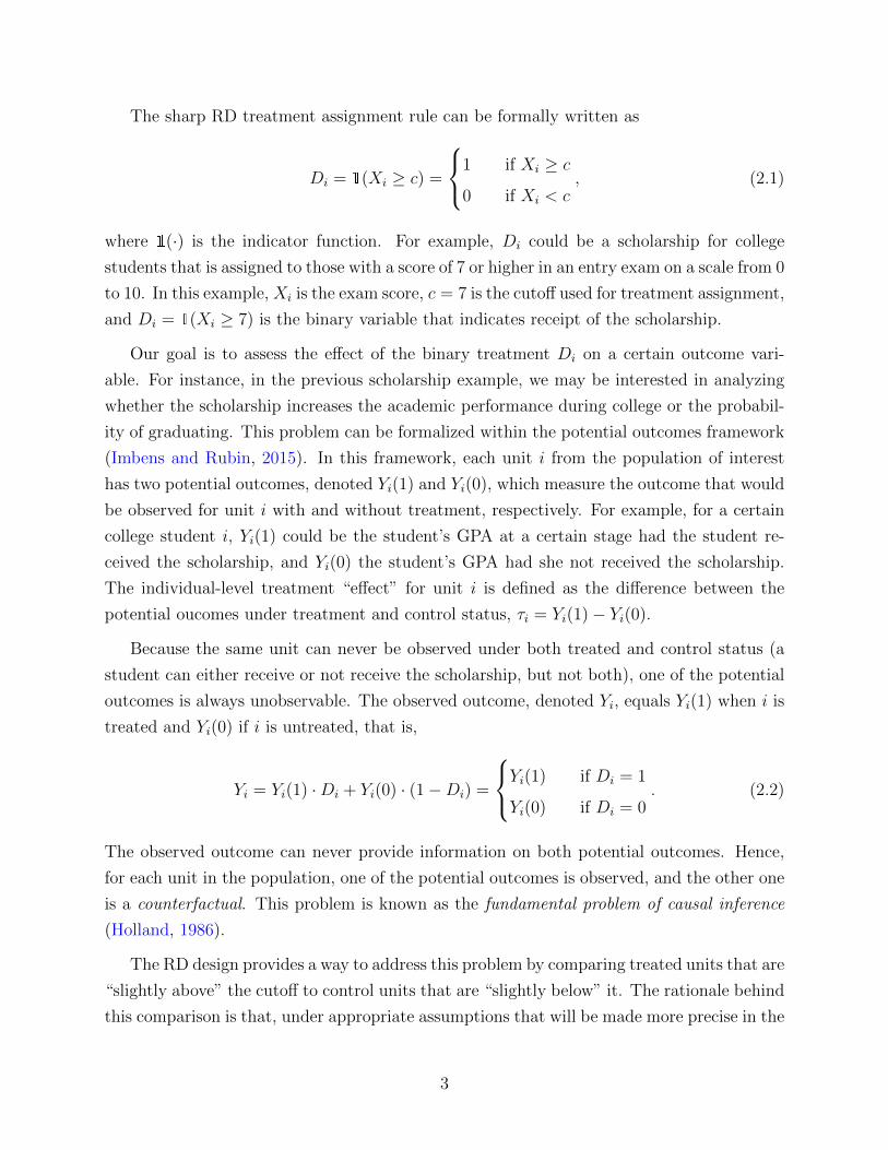
The sharp RD treatment assignment rule can be formally written as

Di = 1(Xi ≥ c) =

1 if Xi ≥ c

0 if Xi < c, (2.1)

where 1(·) is the indicator function. For example, Di could be a scholarship for college

students that is assigned to those with a score of 7 or higher in an entry exam on a scale from 0

to 10. In this example, Xi is the exam score, c = 7 is the cutoff used for treatment assignment,

and Di = 1(Xi ≥ 7) is the binary variable that indicates receipt of the scholarship.

Our goal is to assess the effect of the binary treatment Di on a certain outcome vari-

able. For instance, in the previous scholarship example, we may be interested in analyzing

whether the scholarship increases the academic performance during college or the probabil-

ity of graduating. This problem can be formalized within the potential outcomes framework

(Imbens and Rubin, 2015). In this framework, each unit i from the population of interest

has two potential outcomes, denoted Yi(1) and Yi(0), which measure the outcome that would

be observed for unit i with and without treatment, respectively. For example, for a certain

college student i, Yi(1) could be the student’s GPA at a certain stage had the student re-

ceived the scholarship, and Yi(0) the student’s GPA had she not received the scholarship.

The individual-level treatment “effect” for unit i is defined as the difference between the

potential oucomes under treatment and control status, τi = Yi(1)− Yi(0).

Because the same unit can never be observed under both treated and control status (a

student can either receive or not receive the scholarship, but not both), one of the potential

outcomes is always unobservable. The observed outcome, denoted Yi, equals Yi(1) when i is

treated and Yi(0) if i is untreated, that is,

Yi = Yi(1) ·Di + Yi(0) · (1−Di) =

Yi(1) if Di = 1

Yi(0) if Di = 0. (2.2)

The observed outcome can never provide information on both potential outcomes. Hence,

for each unit in the population, one of the potential outcomes is observed, and the other one

is a counterfactual. This problem is known as the fundamental problem of causal inference

(Holland, 1986).

The RD design provides a way to address this problem by comparing treated units that are

“slightly above” the cutoff to control units that are “slightly below” it. The rationale behind

this comparison is that, under appropriate assumptions that will be made more precise in the

3

upcoming sections, treated and control units in a small neighborhood or window around the

cutoff are comparable in the sense of having similar observed and unobserved characteristics

(with the only exception being treatment status). Thus, observing the outcomes of units

just below the cutoff provides a valid measure of the average outcome that treated units just

above the cutoff would have had if they had not received the treatment.

In the remainder of this chapter, we describe two alternative approaches for analyzing

RD designs. The first one, which we call the continuity-based framework, assumes that

the observed sample is a random draw from an infinite population of interest, and invokes

assumptions of continuity. In this framework, identification of the parameter of interest,

defined precisely in the next section, relies on assuming that the average potential outcomes

given the score are continuous as a function of the score. This assumption implies that

the researcher can compare units marginally above the cutoff to units marginally below to

identify (and estimate) the average treatment effect at the cutoff.

The second approach for RD analysis, which we call the local randomization framework,

assumes that the treatment of interest is as-if randomly assigned in a small region around the

cutoff. This approach formalizes the interpretation of RD designs as local experiments, and

allows researchers to use the standard tools from the classical analysis of experiments. In

addition, if the researcher is willing to assume that potential outcomes are fixed (non-random)

and that the n units that are observed in the sample conform the finite population of interest,

this approach also allows the researcher to use finite-sample exact randomization inference

tools, which are specially appealing in applications where the number of observations near

the cutoff is small.

For both frameworks, we discuss the parameters of interest, estimation, inference, and

bandwidth or window selection methods. We then compare the two approaches and provide

a series of falsification methods that are commonly employed to assess the validity of the RD

design. See also Cattaneo, Titiunik and Vazquez-Bare (2017) for an overview and practical

comparisons between these RD approaches.

3 The Continuity-Based Framework

Under the continuity-based framework, the observed data {Yi(1), Yi(0), Xi, Di}, for i =

1, 2, . . . , n, is a random sample from an infinite population of interest (or data generating

process). The main objects of interest under this framework are the conditional expectation

4

functions of the potential outcomes,

µ1(x) = E[Yi(1)|Xi = x] and µ0(x) = E[Yi(0)|Xi = x], (3.1)

which capture the population average of the potential outcomes for each value of the score.

In the sharp RD design, for each value of x, only one of these functions is observed: µ1(x) is

observed for x at or above the cutoff, and µ0(x) is observed for values of x below the cutoff.

The observed conditional expectation function is

µ(x) = E[Yi|Xi = x] =

µ1(x) if x ≥ c

µ0(x) if x < c.(3.2)

We start by defining the function τ(x), which gives the average treatment effect condi-

tional on Xi = x:

τ(x) = E[Yi(1)− Yi(0)|Xi = x] = µ1(x)− µ0(x). (3.3)

The first step is to establish conditions for identification, that is, conditions under which

we can write the parameter of interest, which depends on unobservable quantities due to

the fundamental problem of causal inference, in terms of observable (i.e., identifiable) and

thus estimable quantities. In the continuity-based framework, the key assumption for iden-

tification is that µ1(x) and µ0(x) are continuous functions of the score at the cutoff point

x = c. Intuitively and informally, this condition states that the observable and unobservable

characteristics that determine the average potential outcomes do not jump abruptly at the

cutoff. When this assumption holds, the only difference between units on opposite sides of

the cutoff whose scores are “very close” to the cutoff is their treatment status.

Intuitively, we can think that treated and control units with very different score values will

generally be very different in terms of important observable and unobservable characteristics

affecting the outcome of interest but, as their scores approach the cutoff and become similar

in that dimension, the only remaining difference between them will be their treatment status,

thus ensuring comparability between units just above and just below the cutoff, at least in

terms of their potential outcome mean regression functions.

More formally, Hahn, Todd and van der Klaauw (2001) showed that, when conditional

expectation functions are continuous in x at the cutoff level x = c,

τ(c) = limx↓c

E[Yi|Xi = x]− limx↑c

E[Yi|Xi = x], (3.4)

5

so that the difference between average observed outcomes for units just above and just below

the cutoff is equal to the average treatment effect at the cutoff, τ(c) = E[Yi(1)−Yi(0)|Xi = c].

Note that this identification result expresses the estimand τ(c), which is unobservable, as a

function of two limits that depend only on observable (i.e., identifiable) quantities that are

estimable from the data.

As a consequence, in a sharp RD design, a natural parameter of interest is τ(c), the

average treatment effect at the cutoff. This parameter captures the average effect of the

treatment on the outcome of interest, given that the value of the score is equal to the cutoff.

It is useful to compare this parameter to the average treatment effect, ATE = E[Yi(1)−Yi(0)],

which is the difference that we would see in average outcomes if all units were switched from

control to treatment. In contrast to ATE, which is a weighted average of τ(x) over x because

ATE = E[τ(Xi)], τ(c) is only the average effect of the treatment at a particular value of the

score, x = c. For this reason, the RD parameter of interest τ(c) is often referred to as a local

average treatment effect, because it is only informative of the effect of the treatment for units

whose value of the score is at (or, loosely speaking, in a local neighborhood of) the cutoff.

This limits the external validity of the RD parameter τ(c). A recent and growing literature

studies how to extrapolate treatment effects in RD designs (Angrist and Rokkanen, 2015;

Dong and Lewbel, 2015; Cattaneo, Keele, Titiunik and Vazquez-Bare, 2016a; Bertanha and

Imbens, 2019; Cattaneo, Keele, Titiunik and Vazquez-Bare, 2020c).

The main advantage of the identification result in (3.4) is that it relies on continuity

conditions of µ1(x) and µ0(x) at x = c, which are nonparametric in nature and reasonable in

a wide array of empirical applications. Section 5 describes several falsification strategies to

provide indirect empirical evidence to assess the plausibility of this assumption. Assuming

continuity holds, the estimation of the RD parameter τ(c) can proceed without making

parametric assumptions about the particular form of E[Yi|Xi = x]. Instead, estimation can

proceed by using nonparametric methods to approximate the regression function E[Yi|Xi =

x], separately for values of x above and below the cutoff.

However, estimation and inference via nonparametric local approximations near the cutoff

is not without challenges. When the score is continuous, there are in general no units with

value of the score exactly equal to the cutoff. Thus, estimation of the limits of E[Yi|Xi = x]

as x tends to the cutoff from above or below will necessarily require extrapolation. To this

end, estimation in RD designs requires specifying a neighborhood or bandwidth around the

cutoff in which to approximate the regression function E[Yi|Xi = x], and then, based on

that approximation, calculate the value that the function has exactly at x = c. In what

follows, we describe different methods for estimation and bandwidth selection under the

6

continuity-based framework.

3.1 Bandwidth Selection

Selecting the bandwidth around the cutoff in which to estimate the effect is a crucial step

in RD analysis, as the results and conclusions are typically sensitive to this choice. We

now briefly outline some common methods for bandwidth selection in RD designs. See also

Cattaneo and Vazquez-Bare (2016) for an overview of neighborhood selection methods in

RD designs.

The approach for bandwidth selection used in early RD studies is what we call ad-hoc

bandwidth selection, in which the researcher chooses a bandwidth without a systematic

data-driven criterion, perhaps relying on intuition or prior knowledge about the particular

context. This approach is not recommended since it lacks objectivity, does not have a rigorous

justification and, by leaving bandwidth selection to the discretion of the researcher, opens

the door for specification searches. For these reasons, the ad-hoc approach to bandwidth

selection has been replaced by systematic, data-driven criteria.

In the RD continuity-based framework, the most widely used bandwidth selection cri-

terion in empirical practice is the mean squared error (MSE) criterion (Imbens and Kalya-

naraman, 2012; Calonico, Cattaneo and Titiunik, 2014b; Arai and Ichimura, 2018; Calonico,

Cattaneo, Farrell and Titiunik, 2019b), which relies on a tradeoff between the bias and vari-

ance of the RD point estimator. The bandwidth determines the neighborhood of observations

around the cutoff that will be used to approximate the unknown function E[Yi|Xi = x] above

and below the cutoff. Intuitively, choosing a very small bandwidth around the cutoff will

tend to reduce the misspecification error in the approximation, thus reducing bias. A very

small bandwidth, however, requires discarding a large fraction of the observations and hence

reduces the sample, leading to estimators with larger variance. Conversely, choosing a very

large bandwidth allows the researcher to gain precision using more observations for estima-

tion and inference, but at the expense of a larger misspecification error, since the function

E[Yi|Xi = x] now has to be approximated over a larger range. The goal of bandwidth se-

lection methods based on this tradeoff is therefore to find the bandwidth that optimally

balances bias and variance.

We let τ denote a local polynomial estimator of the RD treatment effect τ(c)—we explain

how to construct this estimator in the next section. For a given bandwidth h and a total

7

sample size n, the MSE of τ is

MSE(τ) = Bias2(τ) + Variance(τ) = B2 + V , (3.5)

which is the sum of the squared bias and the variance of the estimator. The MSE-optimal

bandwidth, hMSE, is the value of h that balances bias and variance by minimizing the MSE

of τ ,

hMSE = arg minh>0

MSE(τ). (3.6)

The shape of the MSE depends on the specific estimator chosen. For example, when τ

is obtained using local linear regression (LLR), which will be discussed in the next section,

the MSE can be approximated by

MSE(τ) ≈ h4B2 +1

nhV

where B and V are constants that depend on the data generating process and specific features

of the estimator used. This expression clearly highlights how a smaller bandwidth reduces the

bias term while increasing the variance and vice versa. In this case, the optimal bandwidth,

simply obtained by setting the derivative of the above expression with respect to h equal to

zero, is

hLLRMSE = CMSE · n−1/5, (3.7)

where the constant CMSE = (V/(4B2))1/5 is unknown but estimable. This shows that the

MSE-optimal bandwidth for a local linear estimator is proportional to n−1/5.

While hMSE is optimal for point estimation, it is generally not optimal for conducting

inference. Calonico, Cattaneo and Farrell (2018, 2019a, 2020) show how to choose the

bandwidth to obtain confidence intervals minimizing the coverage error probability (CER).

More precisely, let IC(τ) be an α-level confidence interval for the RD parameter τ(c) based

on the estimator τ . A CER-optimal bandwidth makes the coverage probability as close as

possible to the desired level 1− α:

hCER = arg minh>0

|P[τ(c) ∈ IC(τ)]− (1− α)|. (3.8)

For the case of local linear regression, the CER-optimal h is

hLLRCER = CCER · n−1/4,

8

where again the constant CCER unknown, because depends in part on the data generating

process, but estimable. Hence, the CER-optimal bandwidth is smaller than the MSE-optimal

bandwidth, at least in large samples.

Based on the ideas above, several variations of optimal bandwidth selectors exist, includ-

ing one-sided CER-optimal and MSE-optimal bandwidths with and without accounting for

covariate adjustment, clustering, or other specific features. In all cases, these bandwidth

selectors are implemented in two steps: first the constant (e.g., CMSE or CCER) is estimated,

and then the bandwidth is chosen using that preliminary estimate and the appropriate rate

formula (e.g., n−1/5 or n−1/4).

3.2 Estimation and Inference

Given a bandwidth h, continuity-based estimation in RD designs consists on estimating the

outcome regression functions, given the score, separately for treated and control units whose

scores are within the bandwidth. Recall from Equation (3.4) that we need to estimate the

limits of the conditional expectation function of the observed outcome from the right and

from the left.

One possible approach would be to simply estimate the difference in average outcomes

between treated and controls within h. This strategy is equivalent to fitting a regression

including only an intercept at each side of the cutoff. However, since the goal is to estimate

two boundary points, this local constant approach will have a bias that can be reduced

by including a slope term in the regression. More generally, the most common approach

for point estimation in the continuity-based RD framework is to employ local polynomial

methods (Fan and Gijbels, 1996), which involve fitting a polynomial of order p separately

on each side of the cutoff, only for observations inside the bandwidth. Local polynomial

approximations usually include a weighting scheme that places more weight on observations

that are closer to the cutoff; this weighting scheme is based on a kernel function, which we

denote by K(·).

More formally, the treatment effect is estimated as:

τ = α+ − α−

where α+ is obtained as the intercept from the (possibly misspecified) regression model:

Yi = α+ + β1+(Xi − c) + . . .+ βp+(Xi − c)p + ui

9

on the treated observations using weights K((Xi − c)/h), and similarly α− is obtained as

the intercept from an analogous regression fit employing only the control observations. Al-

though theoretically a large value of p can capture more features of the unobserved regression

functions, µ1(x) and µ0(x), in practice high-order polynomials can have erratic behavior, es-

pecially when estimating boundary points, a fact usually known as Runge’s phenomenon

(Calonico, Cattaneo and Titiunik, 2015a, p. 1756-57). In addition, global polynomials can

lead to counter-intuitive weighting schemes, as discussed by Gelman and Imbens (2019).

Common choices for p are p = 1 or p = 2.

As we can see, once the bandwidth has been appropriately chosen, the implementation of

local polynomial regression reduces to simply fitting two linear or quadratic regressions via

weighted least-squares—see Cattaneo, Idrobo and Titiunik (2019) for an extended discussion

and practical introduction. Despite the implementation and algebraic similarities between

ordinary least squares (OLS) methods and local polynomial methods, there is a crucial

difference: OLS methods assume that the polynomial used for estimation is the true form of

the function, while local polynomial methods see it as just an approximation to an unknown

regression function. Thus, inherent in the use of local polynomial methods is the idea that

the resulting estimate will contain a certain error of approximation or misspecification bias.

This difference between OLS and local polynomial methods turns out to be very conse-

quential for inference purposes—that is, for testing statistical hypotheses and constructing

confidence intervals. The conventional OLS inference procedure to test the null hypothesis of

no treatment effect at the cutoff, H0 : τ(c) = 0, relies on the assumption that the distribution

of the t-statistic is approximately standard normal in large samples:

τ√V

a∼ N (0, 1), (3.9)

where V is the (conditional) variance of τ , that is, the square of the standard error.

However, this will only occur in cases where the misspecification bias or approximation

error of the estimator τ for τ(c) becomes sufficiently small in large samples, so that the

distribution of the t-statistic is correctly centered at zero. In general, this will not occur in

RD analysis, where the local polynomials are used as a nonparametric approximation device,

and do not make any specific functional form assumptions about the regression functions

µ1(x) and µ0(x), which will be generally misspecified. The general approximation to the

t-statistic in the presence of misspecification error is

τ −B√V

a∼ N (0, 1), (3.10)

10

where B is the (conditional) bias of τ for τ(c). This approximation will be equivalent to the

one in (3.9) only when B/√

V is small, at least in large samples.

More generally, it is crucial to account for the bias B when conducting inference. The

magnitude of the bias depends on the shape of the true regression functions and on the length

of the bandwidth. As discussed before, the smaller the bandwidth, the smaller the bias.

Although the conventional asymptotic approximation in (3.9) will be valid in some special

cases, such as when the bandwidth is small enough, it is not valid in general. In particular,

if the bandwidth chosen for implementation is the MSE-optimal bandwidth discussed in the

prior section, the bias will remain even in large samples, making inferences based on (3.9)

invalid. In other words, the MSE-optimal bandwidth, which is optimal for point estimation,

is too large when conducting inference according to the usual OLS approximations.

Generally valid inferences thus require researchers to use the asymptotic approximation

in (3.10), which contains the bias. In particular, Calonico, Cattaneo and Titiunik (2014b)

propose a way to construct a t-statistic that corrects the bias of the estimator (thus making

the approximation valid for more bandwidth choices, including the MSE-optimal choice) and

simultaneously adjusts the standard errors to account for the variability that is introduced in

the bias correction step—this additional variability is introduced because the bias is unknown

and thus must be estimated. This approach is known as robust bias-corrected inference.

Based on the approximation (3.10), Calonico, Cattaneo and Titiunik (2014b) propose

robust bias-corrected confidence intervals

CIrbc =[ (τ − B

)± 1.96 ·

√Vbc

],

where, in general, Vbc > V because Vbc includes the variability of estimating B with B. In

terms of implementation, the infeasible variance Vbc can be replaced by a consistent estimator

Vbc, which can account for heteroskedasticity and clustering as apprpriate.

Robust bias correction methods for RD designs have been further developed in recent

years. For example, see Calonico, Cattaneo, Farrell and Titiunik (2019b) for robust bias

correction inference in the context of RD designs with covariate adjustments, clustered data,

and other empirically relevant features. In addition, see Calonico, Cattaneo and Farrell

(2018, 2019a, 2020) for theoretical results justifying some of features of robust bias correc-

tion inference. Finally, see Ganong and Jager (2018) and Hyytinen, Merilainen, Saarimaa,

Toivanen and Tukiainen (2018) for two recent applications and empirical comparisons of

robust bias correction methods.

11

Continuity-based framework: summary

1. Key assumptions:

(a) Random potential outcomes drawn from an infinite population

(b) The regression functions are continuous at the cutoff

2. Bandwidth selection:

(a) Systematic, data-driven selection based on non-parametric methods

(b) Optimality criteria: MSE, coverage error

3. Estimation:

(a) Nonparametric local polynomial regression within bandwidth

(b) Choice parameters: order of the polynomial, weighting method (kernel)

4. Inference:

(a) Large-sample normal approximation

(b) Robust, bias corrected

4 The Local Randomization Framework

The local randomization approach to RD analysis provides an alternative to the continuity-

based framework. Instead of relying on assumptions about the continuity of regression

functions and their approximation and extrapolation, this approach is based on the idea

that, close enough to the cutoff, the treatment can be interpreted to be “as good as randomly

assigned”. The intuition is that, if units either have no knowledge of the cutoff or have

no ability to precisely manipulate their own score, units whose scores are close enough

to the cutoff will have the same chance of being barely above the cutoff as barely below

it. If this is true, close enough to the cutoff, the RD design may create experimental-

like variation in treatment assignment. The idea that RD designs create conditions that

resemble an experiment near the cutoff has been present since the origins of the method

(see Thistlethwaite and Campbell, 1960), and has been sometimes proposed as a heuristic

interpretation of continuity-based RD results.

12

Cattaneo, Frandsen and Titiunik (2015) used this local randomization idea to develop

a formal framework, and to derive alternative assumptions for the analysis of RD designs,

which are stronger than the typical continuity conditions. The formal local randomization

framework was further developed by Cattaneo, Titiunik and Vazquez-Bare (2017). The

central idea behind the local randomization approach is to assume the existence of a neigh-

borhood or window around the cutoff where the assignment to being above or below the

cutoff behaves as it would have behaved in an actual experiment. In other words, the local

randomization RD approach makes the assumption that there is a window around the cutoff

where assignment to treatment is as-if experimental.

The formalization of these assumptions requires a more general notation. In prior sec-

tions, we used Yi(Di) to denote the potential outcome under treatment Di, which could be

equal to one (treatment) or zero (control). Since Di = 1(Xi ≥ c), this also allowed the

score Xi to indirectly affect the potential outcomes; moreover, this notation did not prevent

Yi(·) from being a function of Xi, but this was not explicitly noted. We now generalize the

notation to explicitly note that the potential outcomes may be a direct function of Xi, so we

write Yi(Di, Xi). In addition, note that here and in all prior sections we are implicitly assum-

ing that potential outcomes only depend on unit i’s own treatment assignment and running

variable, an assumption known as SUTVA (stable unit treatment value assumption). While

some of the methods described in this section are robust to some violations of the SUTVA,

we impose this assumption to ease exposition. See Cattaneo, Titiunik and Vazquez-Bare

(2017) for more discussion.

To formalize the local randomization RD approach, we assume that there exists a window

W0 around the cutoff where the following two conditions hold:

� Unconfounded Assignment. The distribution function of the score inside the win-

dow, FXi|Xi∈W0(r), does not depend on the potential outcomes, is the same for all units,

and is known:

FXi|Xi∈W0(x) = F0(x), (4.1)

where F0(x) is a known distribution function.

� Exclusion Restriction. The potential outcomes do not depend on the value of the

running variable inside the window, except via the treatment assignment indicator

Yi(d, x) = Yi(d) ∀ i such that Xi ∈ W0. (4.2)

This condition requires the potential outcomes to be unrelated to the score inside the

13

window.

Importantly, these two assumptions would not be satisfied by randomly assigning the

treatment inside W0, because the random assignment of Di inside W0 does not by itself

guarantee that the score and the potential outcomes are unrelated (the exclusion restriction).

For example, imagine a RD design based on elections, where the treatment is the electoral

victory of a political party, the score is the vote share, and the party wins the election if the

vote share is above 50%. Even if, in very close races, election winners were chosen randomly

instead of based on their actual vote share, donors might still believe that districts where

the party obtained a bare majority are more likely to support the party again, and thus they

may donate more money to the races where the party’s vote share was just above 50% than

to races where the party was just below 50%. If donations are effective in boosting the party,

this would induce a positive relationship near the cutoff between the running variable (vote

share) and the outcome of interest (victory in the future election).

The discussion above illustrates why the unconfounded assignment assumption in equa-

tion (4.1) is not enough for a local randomization approach to RD analysis. We must

explicitly assume that the score and the potential outcomes are unrelated inside W0, which

is not implied by (4.1). This issue is discussed in detail by Sekhon and Titiunik (2017),

who use several examples to show that the exclusion restriction in (4.2) is neither implied

by assuming statistical independence between the potential outcomes and the treatment in

W0, nor by assuming that the running variable is randomly assigned in W0. In addition,

see Sekhon and Titiunik (2016) for a discussion of the status of RD designs among obser-

vational studies, and Titiunik (2020) for a discussion of the connection between RD designs

and natural experiments.

4.1 Estimation and Inference within a Known Window

The local randomization conditions (4.1) and (4.2) open new possibilities for RD estimation

and inference. Of course, these conditions are strong and, just like the continuity conditions

in Section 3, they are not implied by the RD treatment assignment rule but rather must be

assumed in addition to it (Sekhon and Titiunik, 2016). Because these assumptions are strong

and are inherently untestable, it is crucial for researchers to provide as much information

as possible regarding their plausibility. We discuss this issue in Section 5, where we present

several strategies for empirical falsification of the RD assumptions.

The key assumption of the local randomization approach is that there exists a neigh-

borhood around the cutoff in which (4.1) and (4.2) hold—implying that we can treat the

14

RD design as a randomized experiment near the cutoff. We denote this neighborhood by

W0 = [c − w, c + w], where c continues to be the RD cutoff, but we now use the nota-

tion w as opposed to h to emphasize that w will be chosen and interpreted differently from

the previous section. Furthermore, to ease the exposition, we start by assuming that W0 is

known, and then discuss how to select W0 based on observable information. This data-driven

window selection step will be crucial in applications, as in most empirical examples W0 is

fundamentally unknown, if it exists at all—but see Hyytinen et al. (2018) for an exception.

Given a window W0, the local randomization framework summarized by assumptions

(4.1) and (4.2) allows us to analyze the RD design employing the standard tools of the

classical analysis of experiments. Depending on the available number of observations inside

the window, the experimental analysis can follow two different approaches. In the Fisherian

approach, also known as a randomization inference approach, potential outcomes are consid-

ered non-random, the assignment mechanism is assumed to be known, and this assignment

is used to calculate the exact finite-sample distribution of a test statistic of interest under

the null hypothesis that the treatment effect is zero for every unit. On the other hand, in

the large-sample approach, the potential outcomes may be fixed or random, the assignment

mechanism need not be known, and the finite-sample distribution of the test statistic is

approximated under the assumption that the number of observations is large. Thus, in con-

trast to the Fisherian approach, in the large-sample approach inferences are based on test

statistics whose finite-sample properties are unknown, but whose null distribution can be

approximated by a Normal distribution under the assumption that the sample size is large

enough.

Below we briefly review both Fisherian and large-sample methods for analysis of RD

designs under a local randomization framework. Fisherian methods will be most useful

when the number of observations near the cutoff is small, which may render large-sample

methods invalid. In contrast, in applications with many observations, large-sample methods

will be the most natural approach, and Fisherian methods can be used as a robustness check.

4.1.1 Fisherian approach

In the Fisherian framework, the potential outcomes are seen as fixed, non-random magnitudes

from a finite population of n units. The information on the observed sample of units i =

1, . . . , n is not seen as a random draw from an infinite population, but as the population of

interest. This feature allows for the derivation of the finite-sample-exact distribution of test

statistics without relying on approximations.

15

We follow the notation in Cattaneo, Titiunik and Vazquez-Bare (2017), adapting slightly

our previous notation. Let X = (X1, . . . , Xn)′ denote the n × 1 column vector collecting

the observed running variable of all units in the sample, and D = (D1, . . . , Dn)′ be the

vector collecting treatment assignments. The non-random potential outcomes for each unit

i are denoted by yi(d, x) where d and x are possible values for Di and Xi. All the potential

outcomes are collected in the vector y(d,x). The vector of observed outcomes is simply the

vector of potential outcomes, evaluated at the observed values of the treatment and running

variable, Y = y(D,X).

Because potential outcomes are assumed non-random, all the randomness in the model

enters through the running variable vector X, and the treatment assignment D which is a

function of it. In what follows, we let the subscript “0” indicate the subvector inside the

neighborhood W0, so that X0, D0 and Y0 denote the vectors of running variables, treatment

assignments and observed outcomes inside W0. Finally, N+0 will denote the number of

observations inside the neighborhood and above the cutoff (treated units inside W0), and

N−0 the number of units in the neighborhood below the cutoff (control units in W0), with

N0 = N+0 + N−0 . Note that using the fixed-potential outcomes notation, the exclusion

restriction becomes yi(d, x) = yi(d), ∀ i in W0 (see assumption 1(b) in Cattaneo, Frandsen

and Titiunik, 2015).

In this Fisherian framework, a natural null hypothesis to test for the presence of a treat-

ment effect is the sharp null of no effect :

Hs0 : yi(1) = yi(0), ∀i in W0.

This sharp null hypothesis states that switching treatment status does not affect potential

outcomes, implying that the treatment does not have an effect on any unit inside the window.

In this context, a hypothesis is sharp when it allows the researcher to impute all the missing

potential outcomes. Thus, Hs0 is sharp because when there is no effect, all the missing

potential outcomes are equal to the observed ones.

Under Hs0, the researcher can impute all the missing potential outcomes and, since the

assignment mechanism is assumed to be known, it is possible to calculate the distribution

of any test statistic T (D0,Y0) to assess how far in the tails the observed statistic falls.

This reasoning provides a way to calculate a p-value for Hs0 that is finite-sample exact and

does not require any distributional approximation. This randomization inference p-value is

obtained by calculating the value of T (D0,Y0) for all possible values of the treatment vector

inside the window D0, and calculating the probability of T (D0,Y0) being larger than the

16

observed value Tobs. See Cattaneo, Frandsen and Titiunik (2015), Cattaneo, Titiunik and

Vazquez-Bare (2017) and Cattaneo, Titiunik and Vazquez-Bare (2016b) for further details

and implementation issues. See also Cattaneo, Idrobo and Titiunik (2020a) for a practical

introduction to local randomization methods.

In addition to testing the null hypothesis of no treatment effect, the researcher may

be interested in obtaining a point estimate for the effect. When condition (4.2) holds, a

difference in means between treated and controls inside the window,

∆ =1

N+0

n∑i=1

YiDi −1

N−0

n∑i=1

Yi(1−Di),

where the sum runs over all observations inside W0, is unbiased for the sample average

treatment effect in W0,

τ0 =1

N0

n∑i=1

(yi(1)− yi(0)).

However, it is important to emphasize that the randomization inference method described

above cannot test hypotheses on τ0 because the null hypothesis that τ0 = 0 is not sharp, that

is, does not allow the researcher to unequivocally impute all the missing potential outcomes,

without further restrictive assumptions, which is a necessary condition to use Fisherian

methods. Hence, under the assumptions imposed so far, hypothesis testing on τ0 has to be

based on asymptotic approximations, as described in Section 4.1.2.

The assumption that the potential outcomes do not depend on the running variable,

stated in Equation (4.2), can be relaxed by assuming a local parametric model for the

relationship between Y0 and X0. Specifically, Cattaneo, Titiunik and Vazquez-Bare (2017)

assume there exists a transformation φ(·) such that the transformed outcomes do not depend

on X0. This transformation could be, for instance, a linear adjustment that removes the

slope whenever the relationship between outcomes and the running variable is assumed to

be linear. The case where potential outcomes do not depend on the running variable is a

particular case in which φ(·) is the identity function. Both inference and estimation can

therefore be conducted using the transformed outcomes when the assumption that potential

outcomes are unrelated is not reasonable, or as a robustness check.

4.1.2 Large-Sample approach

In the most common large-sample approach, we treat potential outcomes as random vari-

ables, and often see the units in the study as a random sample from a larger population.

17

(Though in the Neyman large-sample approach, potential outcomes are fixed; see Imbens

and Rubin (2015) for more discussion.) In addition to the randomness of the potential out-

comes, this approach differs from the Fisherian approach in its null hypothesis of interest.

Given the randomness of the potential outcomes, the focus is no longer on the sharp null

but rather typically on the hypothesis that the average treatment effect is zero. In our RD

context, this null hypothesis can be written as

Hs0 : E[Yi(1)] = E[Yi(0)], ∀i in W0

Inference in this case is based on the usual large-sample methods for the analysis of ex-

periments, relying on usual difference-in-means tests and Normal-based confidence intervals.

See Imbens and Rubin (2015) and Cattaneo et al. (2020a) for details.

4.2 Window Selection

In practice, the window W0 in which the RD design can be seen as a randomized experiment

is not known and needs to be estimated. Cattaneo, Frandsen and Titiunik (2015) propose

a window selection mechanism based on the idea that in a randomized experiment, the

distribution of observed covariates has to be equal between treated and controls. Thus, if

the local assumption is plausible in any window, it should be in a window where we cannot

reject that the pre-determined characteristics of treated and control units are on average

identical.

The idea of this procedure is to select a test statistic that summarizes differences in a

vector of covariates between groups, such as difference-in-means or the Kolmogorov-Smirnov

statistic, and start with an initial “small” window. Inside this initial window, the researcher

conducts a test of the null hypothesis that covariates are balanced between treated and

control groups. This can be done, for example, by assessing whether the minimum p-value

from the tests of differences-in-means for each covariate is larger than some specified level,

or by conducting a joint test using for instance a Hotelling statistic. If the null hypothesis

is not rejected, enlarge the window and repeat the process. The selected window will be

the widest window in which the null hypothesis is not rejected. Common choices for the

test statistic T (D0,Y0) are the difference-in-means between treated and controls, the two-

sample Kolmogorov-Smirnov statistic or the rank sum statistic. The minimum window to

start the procedure should contain enough observations to ensure enough statistical power

to reject the null hypothesis of covariate balance. The appropriate minimum number of

18

observations will naturally depend on unknown, application-specific parameters, but based

on standard power calculations we suggest using no less than approximately 10 observations

in each group.

See Cattaneo, Frandsen and Titiunik (2015) and Cattaneo, Titiunik and Vazquez-Bare

(2017) for methodological details, Cattaneo, Idrobo and Titiunik (2020a) for a practical

introduction, and Cattaneo, Titiunik and Vazquez-Bare (2016b) for software implementation.

Local randomization framework: summary

1. Key assumptions:

(a) There exists a window W0 in which the treatment assignment mechanism

satisfies two conditions:

� Probability of receiving a particular score value in W0 does not depend

on the potential outcomes

� Exclusion restriction or parametric relationship between Y and X in

W0

2. Window selection:

(a) Goal: Find a window where the key assumptions are plausible

(b) Iterative procedure to balance observed covariates between groups

(c) Choice parameters: test statistic, stopping rule

3. Estimation:

(a) Difference in means between treated and controls within neighborhood OR

(b) Flexible parametric modeling to account for the effect of Xi

4. Inference:

(a) Fisherian randomization-based inference or large-sample inference

(b) Conditional on sample and chosen window

(c) Choice parameter: test statistic, randomization mechanism in Fisherian

19

5 Falsification Methods

Every time researchers use an RD design, they must rely on identification assumptions

that are fundamentally untestable, and that do not hold by construction. If we employ a

continuity-based approach, we must assume that the regression functions are smooth func-

tions of the score at the cutoff. If, on the other hand, we employ a local randomization

approach, we must assume that there exists a window where the treatment behaves as if it

had been randomly assigned. These assumptions may be violated for many reasons. Thus, it

is crucial for researchers to provide as much empirical evidence as possible about its validity.

Although testing the assumptions directly is not possible, there are several empirical

regularities that we expect to hold in most cases where the assumptions are met. We discuss

some of these tests below. Our discussion is brief, but we refer the reader to Cattaneo,

Idrobo and Titiunik (2019) for an extensive practical discussion of RD falsification methods,

and additional references.

1. Covariate Balance. If either the continuity or local randomization assumptions hold,

the treatment should not have an effect on any predetermined covariates, that is, on

covariates whose values are realized before the treatment is assigned. Since the treat-

ment effect on predetermined covariates is zero by construction, consistent evidence of

non-zero effects on covariates that are likely to be confounders would raise questions

about the validity of the RD assumptions. For implementation, researchers should

analyze each covariate as if it were an outcome. In the continuity-based approach, this

requires choosing a bandwidth and performing local polynomial estimation and infer-

ence within that bandwidth. Note that the optimal bandwidth is naturally different for

each covariate. In the local randomization approach, the null hypothesis of no effect

should be tested for each covariate using the same choices as used for the outcome. If

the window is chosen using the covariate balance procedure discussed above, the se-

lected window will automatically be a region where no treatment effects on covariates

are found.

2. Density of Running Variable. Another common falsification test is to study the

number of observations near the cutoff. If units cannot manipulate precisely the value

of the score that they receive, we should expect as many observations just above the

cutoff as just below it. In contrast, for example, if units had the power to affect

their score and they knew that the treatment were very beneficial, we should expect

more people just above the cutoff (where the treatment is received) than below it.

In the continuity-based framework, the procedure is to test the null hypothesis that

20

the density of the running variable is continuous at the cutoff (McCrary, 2008), which

can be implemented in a more robust way via the novel density estimator proposed in

Cattaneo, Jansson and Ma (2020b). In the local randomization framework, Cattaneo,

Titiunik and Vazquez-Bare (2017) propose a novel implementation via a finite sample

exact binomial test of the null hypothesis that the number of treated and control

observations in the chosen window is compatible with a 50% probability of treatment

assignment.

3. Alternative cutoff values. Another falsification test estimates the treatment effect

on the outcome at a cutoff value different from the actual cutoff used for the RD treat-

ment assignment, using the same procedures used to estimate the effect in the actual

cutoff but only using observations that share the same treatment status (all treatment

observations if the artificial cutoff is above the real one, or all control observations if

the artificial cutoff is below the real cutoff). The idea is that no treatment effect should

be found at the artificial cutoff, since the treatment status is not changing.

4. Alternative bandwidth and window choices. Another approach is to study the

robustness of the results to small changes in the size of the bandwidth or window. For

implementation, the main analysis is typically repeated for values of the bandwidth

or window that are slightly smaller and/or larger than the values used in the main

analysis. If the effects completely change or disappear for small changes in the chosen

neighborhood, researchers should be cautious in interpreting their results.

6 Empirical Illustration

To illustrate all the RD methods discussed so far, we partially re-analyze the study by Klasnja

and Titiunik (2017). These authors study municipal mayor elections in Brazil between 1996

and 2012, examining the effect of a party’s victory in the current election on the probability

that the party wins a future election for mayor in the same municipality. The unit of analysis

is the municipality, the score is the party’s margin of victory at election t—defined as the

party’s vote share minus the vote share of the party’s strongest opponent, and the treatment

is the party’s victory at t. Their original analysis focuses on the unconditional victory of the

party at t+1 as the outcome of interest. In this illustration, our outcome of interest is instead

the party’s margin of victory at t + 1, which is only defined for those municipalities where

the incumbent party runs for reelection at t + 1. We analyze this effect for the incumbent

party (defined as the that party won election t−1, whatever this party is) in the full sample.

21

Klasnja and Titiunik (2017) discuss the interpretation and validity issues that arise when

conditioning on the party’s decision to re-run, but we ignore such issues here for the purposes

of illustration.

In addition to the outcome and score variables used for the main empirical analysis, our

covariate-adjusted local polynomial methods, window selection procedure, and falsification

approaches employ seven covariates at the municipality level: per-capita GDP, population,

number of effective parties, and indicators for whether each of four parties (the Democratas,

PSDB, PT and PMDB) won the prior (t− 1) election.

We implement the continuity-based analysis with the rdrobust software (Calonico, Cat-

taneo and Titiunik, 2014a, 2015b; Calonico, Cattaneo, Farrell and Titiunik, 2017), the lo-

cal randomization analysis using the rdlocand software (Cattaneo, Titiunik and Vazquez-

Bare, 2016b), and the density test falsification using the rddensity software (Cattaneo,

Jansson and Ma, 2018). The packages can be obtained for R and Stata from https:

//sites.google.com/site/rdpackages/. We do not present the code to conserve space,

but the full code employed is available in the packages’ website. Cattaneo, Idrobo and Titiu-

nik (2019, 2020a) offer a detailed tutorial on how to use these packages, employing a different

empirical illustration.

Falsification Analysis

We start by presenting a falsification analysis. In order to falsify the continuity-based analy-

sis, we analyze the density of the running variable, and also the effect of the RD treatment on

several predetermined covariates. We start by reporting the result of a continuity-based den-

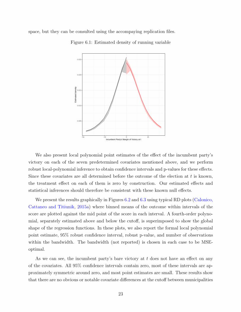
sity test, using the local polynomial density estimator developed by Cattaneo, Jansson and

Ma (2020b). The estimated difference in the density of the running variable at the cutoff is

−0.0753, and the p-value associated with the test of the null hypothesis that this difference

is zero is 0.94. This test is illustrated in Figure 6.1, which shows the local-polynomial-

estimated density of the incumbent party’s margin of victory at t at the cutoff, separately

estimated from above and below the cutoff. These results indicate that the density of the

running variable does not change abruptly at the cutoff, and are thus consistent with the

assumption that parties do not precisely manipulate their margin of victory to ensure a win

in close races.

In addition, we also implemented the finite sample exact binomial tests proposed in

Cattaneo, Titiunik and Vazquez-Bare (2017), which confirmed the empirical results obtained

via local polynomial density methods. We do not report these numerical result to conserve

22

https://sites.google.com/site/rdpackages/

https://sites.google.com/site/rdpackages/

space, but they can be consulted using the accompaying replication files.

Figure 6.1: Estimated density of running variable

0.005

0.010

0.015

0.020

0.025

−50 −25 0 25

Incumbent Party's Margin of Victory at t

Est

imat

ed d

ensi

ty

We also present local polynomial point estimates of the effect of the incumbent party’s

victory on each of the seven predetermined covariates mentioned above, and we perform

robust local-polynomial inference to obtain confidence intervals and p-values for these effects.

Since these covariates are all determined before the outcome of the election at t is known,

the treatment effect on each of them is zero by construction. Our estimated effects and

statistical inferences should therefore be consistent with these known null effects.

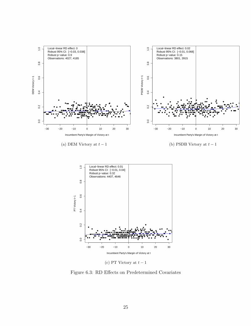
We present the results graphically in Figures 6.2 and 6.3 using typical RD plots (Calonico,

Cattaneo and Titiunik, 2015a) where binned means of the outcome within intervals of the

score are plotted against the mid point of the score in each interval. A fourth-order polyno-

mial, separately estimated above and below the cutoff, is superimposed to show the global

shape of the regression functions. In these plots, we also report the formal local polynomial

point estimate, 95% robust confidence interval, robust p-value, and number of observations

within the bandwidth. The bandwidth (not reported) is chosen in each case to be MSE-

optimal.

As we can see, the incumbent party’s bare victory at t does not have an effect on any

of the covariates. All 95% confidence intervals contain zero, most of these intervals are ap-

proximately symmetric around zero, and most point estimates are small. These results show

that there are no obvious or notable covariate differences at the cutoff between municipalities

23

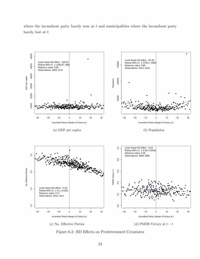
where the incumbent party barely won at t and municipalities where the incumbent party

barely lost at t.

● ●

●●

●

●● ●

●●

●

●●

●

●●

●●

●

●●

●●

●

●

●

●

●●

●

●●

●

●●

●●

●

●●

●●

●●

●●●

●●

●

●

●

●

●

●●

●

●

●●●

●

●●●

●●●

●

●

●

●

●

●

●●●●●●

●

●●

●●

●●

●

●

●

●●

●●

●

●●

●

●

●

●●

●

●●●

●

●

●

●●●●

●

●

●

●●

●

●●

●●

●

●

●

●

●

●

●●

●

●●

●●

●

●●●

●

●●

●

●

●

●●●

●●

●

●

●●●

●

●●

●

●●●

●●●

●●●●●

●

●

●

●

●

●●

●

●

●

●●

●

●

●

●

●

●

●●●

●

●

●

●

●

●

●

●

●

●

●

●

●●

●

●●

●

●

●

●

●

●

●

●●

●

●●

●●

●●●●

●

●

●

●●

●

●●

●

●

●

●

●

●●

●●

●●●

●●

●●

●

●

●

●●

●

● ●●

●

●

●

−30 −20 −10 0 10 20 30

1000

020

000

3000

040

000

5000

060

000


GD

P p

er c

apita

Local−linear RD effect: −150.03Robust 95% CI: [−1205.87, 990]Robust p−value: 0.85Observations: 3628, 3741

(a) GDP per capita

●●

●

●

●

●

●

●

●

●

●

●

●

●

●

●

●

●

●

●

●

●

●

●●

●

●

●●

●●●

●

●

●●

●

●

●●●

●

●

●●

●

●

●

●

●

●●●

●

●

●

●●

●

●●●●

●

●

●

●

●

●●●

●●

●

●●

●

●●

●

●

●

●

●

●

●

●●

●

●

●

●

●

●

●

●

●●

●●●●

●

●●

●

●

●

●

●

●

●●●●

●●

●

●

●

●●

●●

●

●

●

●●●●●●●●

●●

●

●●

●

●●

●●

●

●

●

●

●

●●

●●

●

●

●●

●

●

●●

●

●

●

●

●

●

●

●

●

●

●

●

●

●●

●

●●

●●

●●●

●●

●

●●●

●

●

●

●

●●

●

●

●

●

●

●●

●

●

●

●

●

●

●

●

●

●

●●

●

●●●

●

●●●●●

●

●

●

●

●

●

●

●

●

●

●

●

●

●

●

●●●

●

●

●

●●

●

●

●

●

●

●

●

●

●

●

●

●

●

●

●

●

●

●

−30 −20 −10 0 10 20 3050

000

1000

0015

0000


Pop

ulat

ion

Local−linear RD effect: −26.43Robust 95% CI: [−3793.2, 4500]Robust p−value: 0.86Observations: 2513, 2543

(b) Population

●

●● ● ●

●●

● ● ●

●

●

●

●

●

●

●●

●

●

●●

●

●●●

●

●

●

●

●

●

●

●

●

●

●

●●

●

●

●

●●

●●●

●

●●

●

●

●●

●

●

●

●

●

●

●

●●

●

●

●

●

●

●●

●●

●

●

●

●

●

●●●

●

●

●

●

●

●

●

●

●

●●

●

●

●

●

●●

●

●

●

●

●

●

●

●

●

●

●

●

●

●

●

●

●

●

●

●

●

●●●

●

●

●●

●

●

●●

●

●

●●

●

●

●

●

●

●

●

●

●●●●

●

●

●●

●

●

●

●

●●●●●

●●●●●

●

●

●

●

●

●

●

●●

●

●

●

●

●●●

●●

●

●

●

●

●●●●

●●

●

●

●

●

●

●

●

●

●

●

●

●

●

●

●

●

●

●

●

●

●

●

●

●

●

●●

●

●

●

●

●

●

●

●●

●

●

●

●●

●

●

●

●

●●

●

●

●

●

●

●

●

●

●

●

●●

●●●

●

●

●

●●

●

●

●

●

●

●

●

●●

●

●

●●

●

●

●

●

●

●

●●

●

●

●

●

●●

●

●

●

●

●●

●

●

●

●

●

●

●

●

●●

●

●●

●

●●

●

●●

●

●

●

●

●

●●●

●●●●●

●

●●●●

●●●●●●

●

●

●

●

●

●

●

●

●

●

●

●

●

●

●●●

●●●●

●

●

●

●

●

●●●

●

●●

●

●●

●

●

●

●

●

−30 −20 −10 0 10 20 30

1.0

1.5

2.0

2.5


No.

Effe

ctiv

e P

artie

s

Local−linear RD effect: −0.04Robust 95% CI: [−0.1, 0.018]Robust p−value: 0.17Observations: 3314, 3411

(c) No. Effective Parties

● ●

●

● ●

●

●

●

●

●

●

●●

●

●

●

●

●

●

●

●

●

●●

●

●●

●

●

●

●

●

●

●

●

●

●

●

●

●

●

●

●

●●

●

●

●

●

●

●

●

●

●

●

●

●●

●

●

●

●

●

●●

●

●

●●

●●

●

●

●

●

●

●

●●

●

●

●

●●

●

●

●

●

●

●●

●

●

●

●

●●

●

●

●

●

●●

●

●

●

●

●

●

●

●●

●

●

●

●

●

●●●

●

●

●

●

●

●

●

●

●

●

●

●●

●

●

●

●

●

●

●

●

●●●

●

●

●●

●

●

●

●

●

●

●

●

●

●

●

●

●

●●●●

●

●

●

●

●

●

●

●

●●

●

●

●

●

●

●

●

●

●

●

●

●

●

●

●●●

●

●

●

●

●

●●

●

●

●

●

●

●

●

●

●

●

●

●

●

●

●●

●●

●

●

●

●

●

●

●●

●●

●

●

●

●●

●

●

●

●●●●

●

●

●

●

●

●

●

●●

●

●

●

●

●

●

●

●

●

●●

● ● ●

●

●

● ●

−30 −20 −10 0 10 20 30

0.0

0.2

0.4

0.6

0.8

1.0


PM

DB

Vic

tory

t−1

Local−linear RD effect: −0.03Robust 95% CI: [−0.09, 0.0059]Robust p−value: 0.09Observations: 3838, 3962

(d) PMDB Victory at t− 1

Figure 6.2: RD Effects on Predetermined Covariates

24

●

●

●

●

●

●

●

●

● ●

●●●

●●●

●

●●

●

●

●

●

●

●

●

●

●

●

●

●●

●

●

●

●●●

●

●

●●

●

●

●

●

●

●

●●

●

●

●

●●

●

●

●●

●

●

●

●

●

●

●

●

●

●

●●

●

●

●

●●●●

●●

●

●

●●●

●

●

●●

●

●

●●

●

●

●

●

●

●

●

●●

●●

●

●

●

●

●

●

●●

●

●

●

●

●●

●

●

●

●

●

●

●

●

●

●

●

●

●

●

●●

●●

●

●

●

●

●

●

●

●

●

●

●

●

●

●

●

●

●

●

●

●

●

●

●

●

●

●

●

●

●

●

●

●

●

●

●

●

●

●●

●

●

●

●●●

●

●

●

●●●

●

●

●

●●●

●

●

●

●

●●

●

●

●

●

●

●

●

●

●

●

●

●●●

●

●

●

●

●

●

●

●

●

●

●

●

●

●●

●

●

●

●

●

●●●

●

●●

●

●

●

●

●

●

●●

●

●

●

●

●

●

●

●

●●

●●

●

●

●

●

●

●

●

−30 −20 −10 0 10 20 30

0.0

0.2

0.4

0.6

0.8

1.0


DE

M V

icto

ry t−

1

Local−linear RD effect: 0Robust 95% CI: [−0.03, 0.038]Robust p−value: 0.9Observations: 4027, 4185

(a) DEM Victory at t− 1

●

●

●

●

●

● ●

●

●

●

●

●

●

●

●●

●

●

●

●

●

●

●

●

●

●

●

●

●

●

●

●

●

●

●

●●

●

●

●

●

●

●●

●●

●

●

●

●

●

●●

●

●

●

●

●●

●

●●

●

●

●

●

●

●

●

●

●

●

●

●

●

●

●

●●●

●

●

●

●

●

●

●

●●

●

●

●

●

●

●

●

●

●

●

●

●

●

●

●

●

●

●

●

●

●

●

●

●●

●

●

●

●

●

●

●

●

●

●

●

●

●

●

●

●

●

●

●

●●

●

●

●●

●

●

●

●●

●●

●

●

●

●

●●

●

●

●

●

●

●

●

●

●

●

●

●

●

●

●

●

●

●

●

●

●

●

●

●

●●

●

●

●

●

●

●

●

●

●

●

●

●

●

●

●

●

●

●

●

●

●

●

●

●●

●

●

●●●

●

●

●

●

●

●

●

●

●

●

●

●

●

●

●

●

●

●

●

●

●●

●

●

●

●

●

●

●

●

●●

●

●

●

●

●

●

●

●

●

●

●

●

●●●

●

●

●

●

●

●

●

●

●

−30 −20 −10 0 10 20 30

0.0

0.2

0.4

0.6

0.8

1.0


PS

DB

Vic

tory

t−1

Local−linear RD effect: 0.02Robust 95% CI: [−0.01, 0.068]Robust p−value: 0.15Observations: 3801, 3915

(b) PSDB Victory at t− 1

●

●

●

●

●

●

●

● ● ●

●

●

●

●●

●

●

●

●

●

●

●

●

●

●

●

●

●

●

●

●

●

●

●●

●

●●

●

●

●

●

●

●

●●

●●

●

●

●

●

●●●●

●

●

●

●●

●

●

●

●

●

●

●

●

●●

●

●

●

●

●●

●

●●

●

●

●

●●

●

●

●

●

●

●

●

●

●

●

●●

●

●

●

●

●

●

●●

●

●

●

●

●●

●●

●

●

●●

●

●

●

●

●

●

●●●

●

●

●

●

●

●●

●

●●

●

●

●

●

●

●

●

●●

●●●

●

●

●

●

●

●●

●

●

●●

●

●

●

●

●

●●●

●

●

●

●

●

●●

●●

●

●

●

●

●

●

●

●

●

●

●

●●

●

●

●

●

●

●

●

●

●

●

●

●

●

●

●

●

●

●

●●

●

●

●

●

●

●

●

●

●

●

●

●●

●

●

●

●

●●

●

●

●

●

●

●

●

●

●

●

●

●●●

●

●

●

●

●

●

●●

●

●

●

●

●

●

●

●

●

●

●

● ●

−30 −20 −10 0 10 20 30

0.0

0.2

0.4

0.6

0.8

1.0


PT

Vic

tory

t−1

Local−linear RD effect: 0.01Robust 95% CI: [−0.01, 0.04]Robust p−value: 0.32Observations: 4407, 4646

(c) PT Victory at t− 1

Figure 6.3: RD Effects on Predetermined Covariates

25

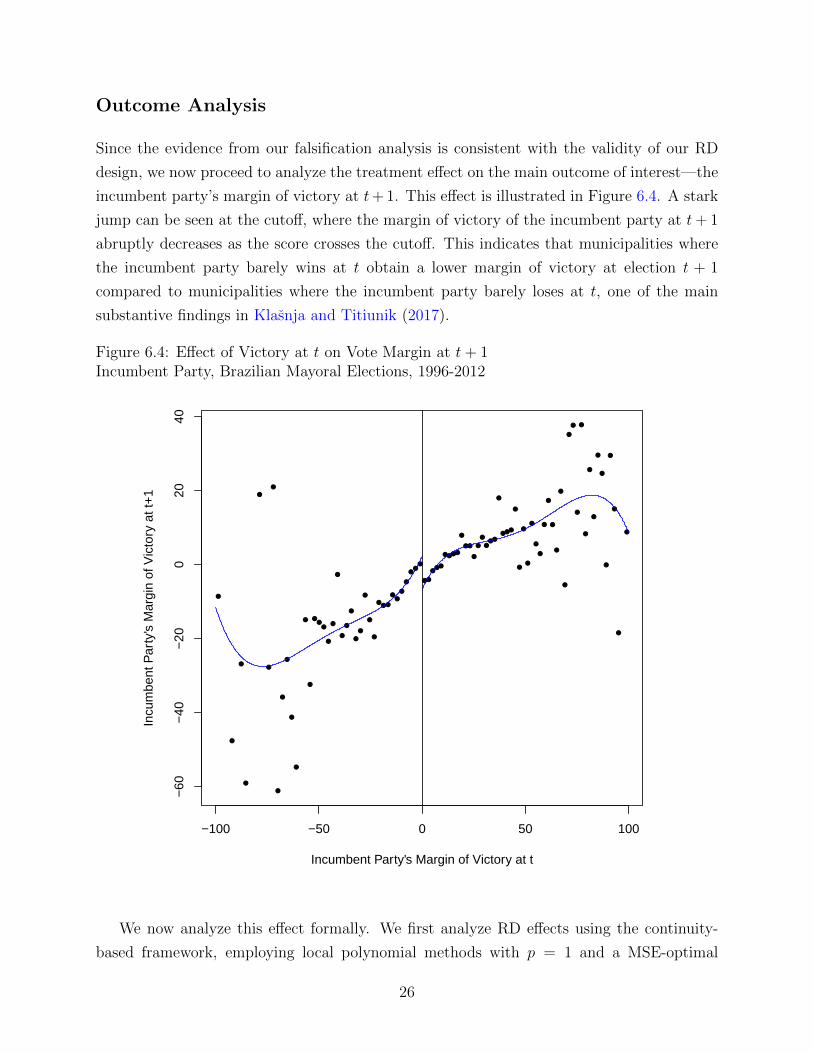
Outcome Analysis

Since the evidence from our falsification analysis is consistent with the validity of our RD

design, we now proceed to analyze the treatment effect on the main outcome of interest—the

incumbent party’s margin of victory at t+ 1. This effect is illustrated in Figure 6.4. A stark

jump can be seen at the cutoff, where the margin of victory of the incumbent party at t+ 1

abruptly decreases as the score crosses the cutoff. This indicates that municipalities where

the incumbent party barely wins at t obtain a lower margin of victory at election t + 1

compared to municipalities where the incumbent party barely loses at t, one of the main

substantive findings in Klasnja and Titiunik (2017).

Figure 6.4: Effect of Victory at t on Vote Margin at t+ 1Incumbent Party, Brazilian Mayoral Elections, 1996-2012

●

●

●

●

●

●

●

●

●

●

●

●

●

●

●●

●

●

●

●

●

●

●

●

●

●

●

●

●●●

●●

●

●

●●

●

●●

●●●

●●●●

●

●●

●

●

●

●●●

●

●●●

●

●

●

●

●

●

●

●

●

●

●

●

●

●

●

●

●

●

●

●

●

●

●

●

●

●

●

−100 −50 0 50 100

−60

−40

−20

020

40


Incu

mbe

nt P

arty

's M

argi

n of

Vic

tory

at t

+1

We now analyze this effect formally. We first analyze RD effects using the continuity-

based framework, employing local polynomial methods with p = 1 and a MSE-optimal

26

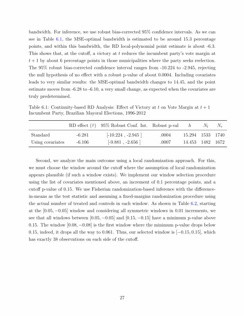
bandwidth. For inference, we use robust bias-corrected 95% confidence intervals. As we can

see in Table 6.1, the MSE-optimal bandwidth is estimated to be around 15.3 percentage

points, and within this bandwidth, the RD local-polynomial point estimate is about -6.3.

This shows that, at the cutoff, a victory at t reduces the incumbent party’s vote margin at

t+ 1 by about 6 percentage points in those municipalities where the party seeks reelection.

The 95% robust bias-corrected confidence interval ranges from -10.224 to -2.945, rejecting

the null hypothesis of no effect with a robust p-value of about 0.0004. Including covariates

leads to very similar results: the MSE-optimal bandwidth changes to 14.45, and the point

estimate moves from -6.28 to -6.10, a very small change, as expected when the covariates are

truly predetermined.

Table 6.1: Continuity-based RD Analysis: Effect of Victory at t on Vote Margin at t+ 1Incumbent Party, Brazilian Mayoral Elections, 1996-2012

RD effect (τ) 95% Robust Conf. Int. Robust p-val h Nl Nr

Standard -6.281 [-10.224 , -2.945 ] .0004 15.294 1533 1740

Using covariates -6.106 [-9.881 , -2.656 ] .0007 14.453 1482 1672

Second, we analyze the main outcome using a local randomization approach. For this,

we must choose the window around the cutoff where the assumption of local randomization

appears plausible (if such a window exists). We implement our window selection procedure

using the list of covariates mentioned above, an increment of 0.1 percentage points, and a

cutoff p-value of 0.15. We use Fisherian randomization-based inference with the difference-

in-means as the test statistic and assuming a fixed-margins randomization procedure using

the actual number of treated and controls in each window. As shown in Table 6.2, starting

at the [0.05,−0.05] window and considering all symmetric windows in 0.01 increments, we

see that all windows between [0.05,−0.05] and [0.15,−0.15] have a minimum p-value above

0.15. The window [0.08,−0.08] is the first window where the minimum p-value drops below

0.15, indeed, it drops all the way to 0.061. Thus, our selected window is [−0.15, 0.15], which

has exactly 38 observations on each side of the cutoff.

27

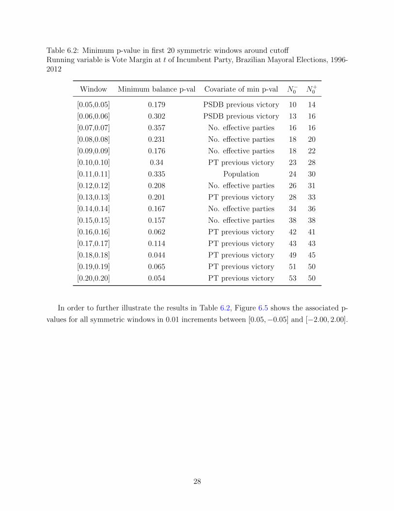
Table 6.2: Minimum p-value in first 20 symmetric windows around cutoffRunning variable is Vote Margin at t of Incumbent Party, Brazilian Mayoral Elections, 1996-2012

Window Minimum balance p-val Covariate of min p-val N−0 N+0

[0.05,0.05] 0.179 PSDB previous victory 10 14

[0.06,0.06] 0.302 PSDB previous victory 13 16

[0.07,0.07] 0.357 No. effective parties 16 16



[0.10,0.10] 0.34 PT previous victory 23 28

[0.11,0.11] 0.335 Population 24 30










In order to further illustrate the results in Table 6.2, Figure 6.5 shows the associated p-

values for all symmetric windows in 0.01 increments between [0.05,−0.05] and [−2.00, 2.00].

28

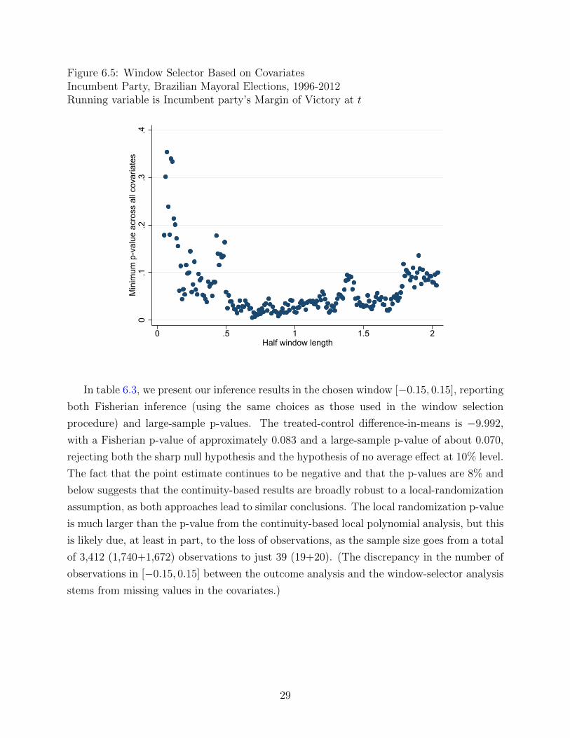
Figure 6.5: Window Selector Based on CovariatesIncumbent Party, Brazilian Mayoral Elections, 1996-2012Running variable is Incumbent party’s Margin of Victory at t

0.1

.2.3

.4M

inim

um p

-val

ue a

cros

s al

l cov

aria

tes

0 .5 1 1.5 2Half window length

In table 6.3, we present our inference results in the chosen window [−0.15, 0.15], reporting

both Fisherian inference (using the same choices as those used in the window selection

procedure) and large-sample p-values. The treated-control difference-in-means is −9.992,

with a Fisherian p-value of approximately 0.083 and a large-sample p-value of about 0.070,

rejecting both the sharp null hypothesis and the hypothesis of no average effect at 10% level.

The fact that the point estimate continues to be negative and that the p-values are 8% and

below suggests that the continuity-based results are broadly robust to a local-randomization

assumption, as both approaches lead to similar conclusions. The local randomization p-value

is much larger than the p-value from the continuity-based local polynomial analysis, but this

is likely due, at least in part, to the loss of observations, as the sample size goes from a total

of 3,412 (1,740+1,672) observations to just 39 (19+20). (The discrepancy in the number of

observations in [−0.15, 0.15] between the outcome analysis and the window-selector analysis

stems from missing values in the covariates.)

29

Table 6.3: Local Randomization RD Analysis: Effect of Victory at t on Vote Margin at t+ 1Incumbent Party, Brazilian Mayoral Elections, 1996-2012

RD effect τ0 Fisher p-val Large-sample p-val Window N−0 N+0

-9.992 0.083 0.0697 [-0.15, 0.15] 19 20

30

7 Final Remarks

We reviewed two alternative frameworks for analyzing sharp RD designs. First, the continuity-

based approach, which is more common in empirical work, assumes that the unknown regres-

sion functions are continuous at the cutoff. Estimation is conducted nonparametrically using

local polynomial methods, and bandwidth selection relies on minimizing a criterion such as

the MSE or the coverage error probability. Inference under this framework relies on large

sample distributional approximations, and requires robust bias correction to account for mis-

specification errors local to the cutoff. Second, the local randomization approach formalizes

the intuition that RD designs can be interpreted as local experiments in a window around

the cutoff. In this case, the window is chosen to ensure that treated and controls are com-

parable in terms of observed predetermined characteristics, as in a randomized experiment.

Within this window, inference is conducted using randomization inference methods assuming

that potential outcomes are non-random, or other canonical analysis of experiments methods

based on large sample approximations.

These two approaches rely on different assumptions, each with its own advantages and

disadvantages, and thus we see them as complementary. On the one hand, the continuity-

based approach is agnostic about the data generating process and does not require any

modeling or distributional assumptions on the regression functions. This generality comes

at the expense of basing inference on large-sample approximations, which may not be reliable

when the sample size is small (a case that is common in RD designs, given their local nature).

On the other hand, the Fisherian local randomization approach provides tools to conduct

inference that is exact in finite samples and does not rely on distributional approximations.

This type of inference is more reliable than large-sample-based inference when the sample

size is small. And if the sample size near the cutoff is large, the analysis can also be

conducted using standard large-sample methods for the analysis of experiments. However,

the conclusions drawn under the local randomization approach (either Fisherian or large-

sample) require stronger assumptions (unconfounded assignment, exclusion restriction) than

the continuity-based approach, are conditional on a specific sample and window, and do not

generalize to other samples or populations.

In sum, as in Cattaneo, Titiunik and Vazquez-Bare (2017), we recommend the continuity-

based approach as the default approach for analysis, since it does not require parametric

modeling assumptions and automatically accounts for misspecification bias in the regression

functions when conducting estimation and inference. The local randomization approach can

be used as a robustness check, especially when the sample size is small and the large-sample

31

approximations may not be reliable.

There is one particular case, however, in which the continuity-based approach is not

applicable: when the running variable exhibits only a few distinct values or mass points

(even if the sample size is large because of repeated values). In this case, the nonparametric

methods for estimation, inference, and bandwidth selection described above do not apply,

since they are developed under the assumption of local approximations and continuity of the

score variable, which are violated by construction when the running variable is discrete with

a small number of mass points. Thus, in settings where the running variable has few mass

points, local randomization methods, possibly employing only the closest observations to the

cutoff, are a more natural approach for analysis. We refer the reader to Cattaneo, Idrobo

and Titiunik (2020a) for a more detailed discussion and practical illustration of this point.

32

Bibliography

Abadie, A., and Cattaneo, M. D. (2018), “Econometric Methods for Program Evaluation,”

Annual Review of Economics, 10, 465–503.

Angrist, J. D., and Rokkanen, M. (2015), “Wanna get away? Regression discontinuity esti-

mation of exam school effects away from the cutoff,” Journal of the American Statistical

Association, 110, 1331–1344.

Arai, Y., and Ichimura, H. (2018), “Simultaneous Selection of Optimal Bandwidths for the

Sharp Regression Discontinuity Estimator,” Quantitative Economics, 9, 441–482.

Bertanha, M., and Imbens, G. W. (2019), “External Validity in Fuzzy Regression Disconti-

nuity Designs,” Journal of Business & Economic Statistics, forthcoming.

Calonico, S., Cattaneo, M. D., and Farrell, M. H. (2018), “On the Effect of Bias Estimation

on Coverage Accuracy in Nonparametric Inference,” Journal of the American Statistical

Association, 113, 767–779.

(2019a), “Coverage Error Optimal Confidence Intervals for Local Polynomial Regres-

sion,” arXiv:1808.01398.

(2020), “Optimal Bandwidth Choice for Robust Bias Corrected Inference in Regres-

sion Discontinuity Designs,” Econometrics Journal, forthcoming.

Calonico, S., Cattaneo, M. D., Farrell, M. H., and Titiunik, R. (2017), “rdrobust: Software

for Regression Discontinuity Designs,” Stata Journal, 17, 372–404.

(2019b), “Regression Discontinuity Designs Using Covariates,” Review of Economics

and Statistics, 101, 442–451.

Calonico, S., Cattaneo, M. D., and Titiunik, R. (2014a), “Robust Data-Driven Inference in

the Regression-Discontinuity Design,” Stata Journal, 14, 909–946.

(2014b), “Robust Nonparametric Confidence Intervals for Regression-Discontinuity

Designs,” Econometrica, 82, 2295–2326.

(2015a), “Optimal Data-Driven Regression Discontinuity Plots,” Journal of the

American Statistical Association, 110, 1753–1769.

(2015b), “rdrobust: An R Package for Robust Nonparametric Inference in

Regression-Discontinuity Designs,” R Journal, 7, 38–51.

33

Cattaneo, M. D., and Escanciano, J. C. (2017), Regression Discontinuity Designs: Theory

and Applications (Advances in Econometrics, volume 38), Emerald Group Publishing.

Cattaneo, M. D., Frandsen, B., and Titiunik, R. (2015), “Randomization Inference in the

Regression Discontinuity Design: An Application to Party Advantages in the U.S. Senate,”

Journal of Causal Inference, 3, 1–24.

Cattaneo, M. D., Idrobo, N., and Titiunik, R. (2019), A Practical Introduction to Regression

Discontinuity Designs: Foundations, Cambridge Elements: Quantitative and Computa-

tional Methods for Social Science, Cambridge University Press.

(2020a), A Practical Introduction to Regression Discontinuity Designs: Extensions,

In preparation for Cambridge Elements: Quantitative and Computational Methods for

Social Science, Cambridge University Press.

Cattaneo, M. D., Jansson, M., and Ma, X. (2018), “Manipulation Testing based on Density

Discontinuity,” Stata Journal, 18, 234–261.

(2020b), “Simple Local Polynomial Density Estimators,” Journal of the American

Statistical Association, forthcoming.

Cattaneo, M. D., Keele, L., Titiunik, R., and Vazquez-Bare, G. (2016a), “Interpreting Re-

gression Discontinuity Designs with Multiple Cutoffs,” Journal of Politics, 78, 1229–1248.

(2020c), “Extrapolating Treatment Effects in Multi-Cutoff Regression Discontinuity

Designs,” arXiv:1808.04416.

Cattaneo, M. D., Titiunik, R., and Vazquez-Bare, G. (2016b), “Inference in Regression

Discontinuity Designs under Local Randomization,” Stata Journal, 16, 331–367.

(2017), “Comparing Inference Approaches for RD Designs: A Reexamination of the

Effect of Head Start on Child Mortality,” Journal of Policy Analysis and Management,

36, 643–681.

Cattaneo, M. D., and Vazquez-Bare, G. (2016), “The Choice of Neighborhood in Regression

Discontinuity Designs,” Observational Studies, 2, 134–146.

Dong, Y., and Lewbel, A. (2015), “Identifying the Effect of Changing the Policy Threshold

in Regression Discontinuity Models,” Review of Economics and Statistics, 97, 1081–1092.

Fan, J., and Gijbels, I. (1996), Local polynomial Modelling and Its Applications, Vol. 66,

CRC Press.

34

Ganong, P., and Jager, S. (2018), “A Permutation Test for the Regression Kink Design,”

Journal of the American Statistical Association, 113, 494–504.

Gelman, A., and Imbens, G. W. (2019), “Why High-Order Polynomials Should Not be Used

in Regression Discontinuity Designs,” Journal of Business & Economic Statistics, 37, 447–

456.

Hahn, J., Todd, P., and van der Klaauw, W. (2001), “Identification and Estimation of

Treatment Effects with a Regression-Discontinuity Design,” Econometrica, 69, 201–209.

Holland, P. W. (1986), “Statistics and Causal Inference,” Journal of the American Statistical

Association, 81, 945–960.

Hyytinen, A., Merilainen, J., Saarimaa, T., Toivanen, O., and Tukiainen, J. (2018), “When

does regression discontinuity design work? Evidence from random election outcomes,”

Quantitative Economics, 9, 1019–1051.

Imbens, G., and Rubin, D. B. (2015), Causal Inference in Statistics, Social, and Biomedical

Sciences, Cambridge University Press.

Imbens, G. W., and Kalyanaraman, K. (2012), “Optimal Bandwidth Choice for the Regres-

sion Discontinuity Estimator,” Review of Economic Studies, 79, 933–959.

Klasnja, M., and Titiunik, R. (2017), “The incumbency curse: Weak parties, term limits,

and unfulfilled accountability,” American Political Science Review, 111, 129–148.

McCrary, J. (2008), “Manipulation of the running variable in the regression discontinuity

design: A density test,” Journal of Econometrics, 142, 698–714.

Sekhon, J. S., and Titiunik, R. (2016), “Understanding Regression Discontinuity Designs as

Observational Studies,” Observational Studies, 2, 174–182.

(2017), “On Interpreting the Regression Discontinuity Design as a Local Experi-

ment,” in Regression Discontinuity Designs: Theory and Applications (Advances in Econo-

metrics, volume 38), eds. M. D. Cattaneo and J. C. Escanciano, Emerald Group Publish-

ing, pp. 1–28.

Thistlethwaite, D. L., and Campbell, D. T. (1960), “Regression-discontinuity Analysis: An

Alternative to the Ex-Post Facto Experiment,” Journal of Educational Psychology, 51,

309–317.

Titiunik, R. (2020), “Natural Experiments,” in Advances in Experimental Political Science,

eds. J. Druckman and D. Green, Cambridge University Press, forthcoming.

35

Documents

The Regression Discontinuity Design