David Goodstein’s Cosmology Book

The Reionization of Cosmic Hydrogenby the First Galaxies

Abraham LoebDepartment of Astronomy, Harvard University, 60 Garden St., Cambridge MA, 02138

Abstract

Cosmology is by now a mature experimental science. We are privileged to live at a time when the story ofgenesis (how the Universe started and developed) can be critically explored by direct observations. Lookingdeep into the Universe through powerful telescopes, we can see images of the Universe when it was youngerbecause of the finite time it takes light to travel to us from distant sources.

Existing data sets include an image of the Universe when it was 0.4 million years old (in the form of thecosmic microwave background), as well as images of individual galaxies when the Universe was older than abillion years. But there is a serious challenge: in between these two epochs was a period when the Universewas dark, stars had not yet formed, and the cosmic microwave background no longer traced the distributionof matter. And this is precisely the most interesting period, when the primordial soup evolved into the richzoo of objects we now see.

The observers are moving ahead along several fronts. The first involves the construction of large infraredtelescopes on the ground and in space, that will provide us with new photos of the first galaxies. Current plansinclude ground-based telescopes which are 24-42 meter in diameter, and NASA’s successor to the HubbleSpace Telescope, called the James Webb Space Telescope. In addition, several observational groups aroundthe globe are constructing radio arrays that will be capable of mapping the three-dimensional distribution ofcosmic hydrogen in the infant Universe. These arrays are aiming to detect the long-wavelength (redshifted21-cm) radio emission from hydrogen atoms. The images from these antenna arrays will reveal how the non-uniform distribution of neutral hydrogen evolved with cosmic time and eventually was extinguished by theultra-violet radiation from the first galaxies. Theoretical research has focused in recent years on predictingthe expected signals for the above instruments and motivating these ambitious observational projects.

1 Introduction

1.1 Observing our past

When we look at our image reflected off a mirror at a distance of 1 meter, we see the way we looked 6.7nanoseconds ago, the light travel time to the mirror and back. If the mirror is spaced 1019 cm ≃ 3 pcaway, we will see the way we looked twenty one years ago. Light propagates at a finite speed, and so byobserving distant regions, we are able to see what the Universe looked like in the past, a light travel timeago (Figure 1). The statistical homogeneity of the Universe on large scales guarantees that what we see faraway is a fair statistical representation of the conditions that were present in in our region of the Universea long time ago.

This fortunate situation makes cosmology an empirical science. We do not need to guess how the Universeevolved. Using telescopes we can simply see how it appeared at earlier cosmic times. In principle, this allowsthe entire 13.7 billion year cosmic history of our universe to be reconstructed by surveying the galaxies andother sources of light to large distances (Figure 2). Since a greater distance means a fainter flux from a sourceof a fixed luminosity, the observation of the earliest sources of light requires the development of sensitiveinstruments and poses challenges to observers.

As the universe expands, photon wavelengths get stretched as well. The factor by which the observedwavelength is increased (i.e. shifted towards the red) relative to the emitted one is denoted by (1+ z), wherez is the cosmological redshift. Astronomers use the known emission patterns of hydrogen and other chemicalelements in the spectrum of each galaxy to measure z. This then implies that the universe has expandedby a factor of (1 + z) in linear dimension since the galaxy emitted the observed light, and cosmologists cancalculate the corresponding distance and cosmic age for the source galaxy. Large telescopes have allowedastronomers to observe faint galaxies that are so far away that we see them more than twelve billion yearsback in time. Thus, we know directly that galaxies were in existence as early as 500 million years after theBig Bang, at a redshift of z ∼ 10 or higher.

1

z = 1100

z = 50

z = 10

z = 1

z = 2

z = 5

Big Bang

Today

Here distance

time

redshift

Hydro

gen

Rec

ombinati

on

Rei

oniz

ation

z = ∞

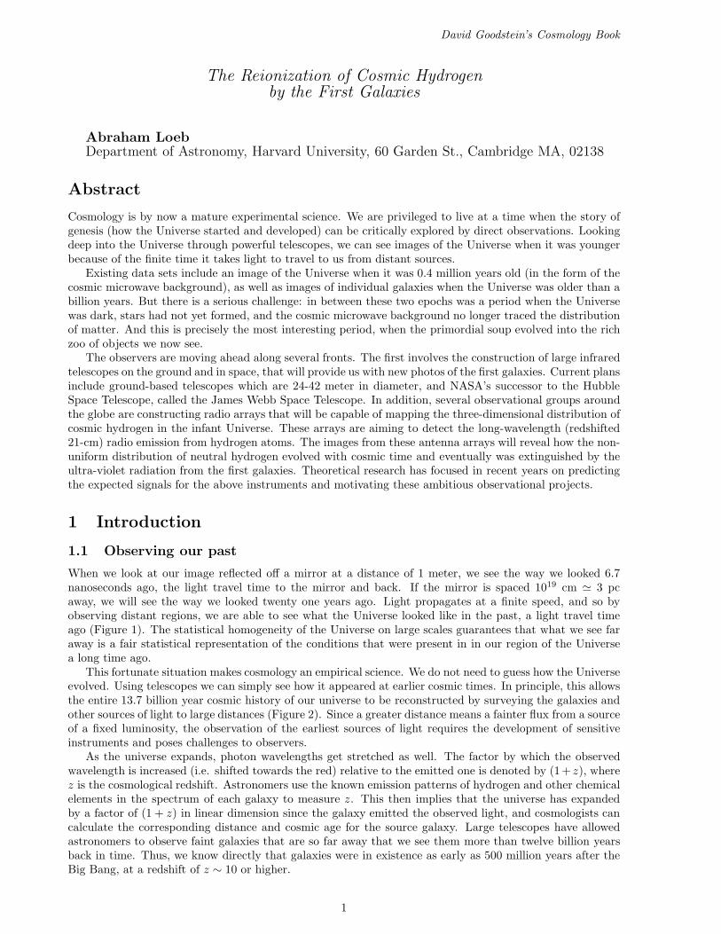
Figure 1: Cosmic archaeology of the observable volume of the Universe, in comoving coordinates (which factorout the cosmic expansion). The outermost observable boundary (z = ∞) marks the comoving distance thatlight has travelled since the Big Bang. Future observatories aim to map most of the observable volume ofour Universe, and improve dramatically the statistical information we have about the density fluctuationswithin it. Existing data on the CMB probes mainly a very thin shell at the hydrogen recombination epoch(z ∼ 103, beyond which the Universe is opaque), and current large-scale galaxy surveys map only a smallregion near us at the center of the diagram. The formation epoch of the first galaxies that culminated withhydrogen reionization at a redshift z ∼ 10 is shaded grey. Note that the comoving volume out to any of theseredshifts scales as the distance cubed. Figure credit: Loeb, A., “How Did the First Stars and GalaxiesForm?”, Princeton University Press (2010).

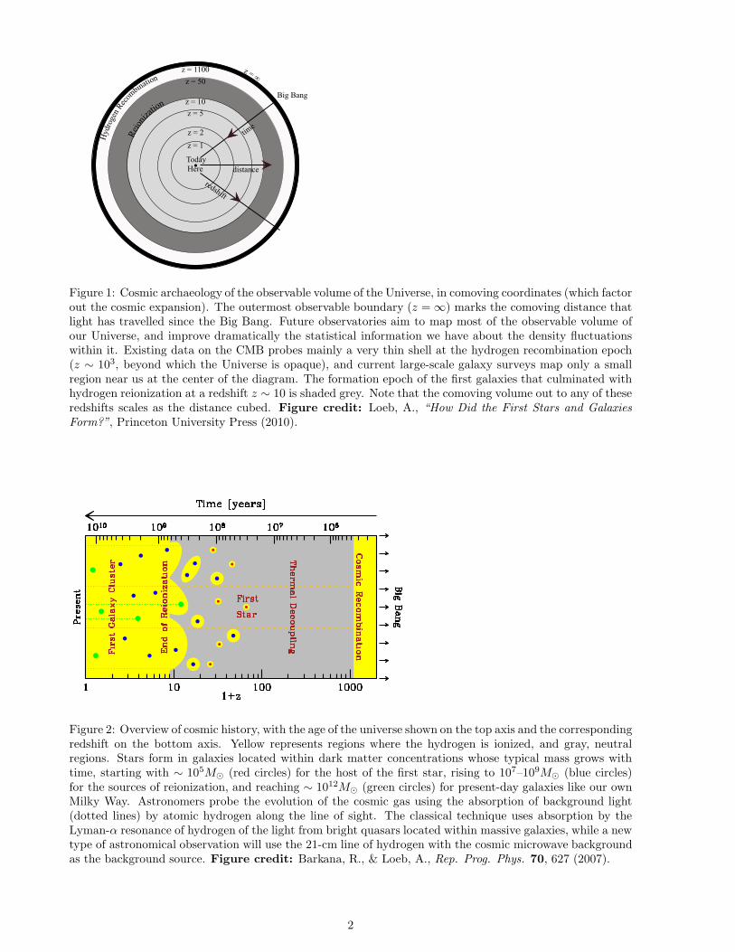
Figure 2: Overview of cosmic history, with the age of the universe shown on the top axis and the correspondingredshift on the bottom axis. Yellow represents regions where the hydrogen is ionized, and gray, neutralregions. Stars form in galaxies located within dark matter concentrations whose typical mass grows withtime, starting with ∼ 105M⊙ (red circles) for the host of the first star, rising to 107–109M⊙ (blue circles)for the sources of reionization, and reaching ∼ 1012M⊙ (green circles) for present-day galaxies like our ownMilky Way. Astronomers probe the evolution of the cosmic gas using the absorption of background light(dotted lines) by atomic hydrogen along the line of sight. The classical technique uses absorption by theLyman-α resonance of hydrogen of the light from bright quasars located within massive galaxies, while a newtype of astronomical observation will use the 21-cm line of hydrogen with the cosmic microwave backgroundas the background source. Figure credit: Barkana, R., & Loeb, A., Rep. Prog. Phys. 70, 627 (2007).

2

We can in principle image the Universe only if it is transparent. Earlier than 400 000 years after the bigbang, the cosmic hydrogen was broken into its constituent electrons and protons (i.e. “ionized”) and theUniverse was opaque to scattering by the free electrons in the dense plasma. Thus, telescopes cannot be usedto electromagnetically image the infant Universe at earlier times (or redshifts > 103). The earliest possibleimage of the Universe was recorded by the COBE and WMAP satellites, which measured the temperaturedistribution of the cosmic microwave background (CMB) on the sky.

The CMB, the relic radiation from the hot, dense beginning of the universe, is indeed another majorprobe of observational cosmology. The universe cools as it expands, so it was initially far denser and hotterthan it is today. For hundreds of thousands of years the cosmic gas consisted of a plasma of free protons andelectrons, and a slight mix of light nuclei, sustained by the intense thermal motion of these particles. Justlike the plasma in our own Sun, the ancient cosmic plasma emitted and scattered a strong field of visibleand ultraviolet photons. As mentioned above, about 400 000 years after the Big Bang the temperature ofthe universe dipped for the first time below a few thousand degrees Kelvin. The protons and electrons werenow moving slowly enough that they could attract each other and form hydrogen atoms, in a process knownas cosmic recombination. With the scattering of the energetic photons now much reduced, the photonscontinued traveling in straight lines, mostly undisturbed except that cosmic expansion has redshifted theirwavelength into the microwave regime today. The emission temperature of the observed spectrum of theseCMB photons is the same in all directions to one part in 100 000, which reveals that conditions were nearlyuniform in the early universe.

It was just before the moment of cosmic recombination (when matter started to dominate in energydensity over radiation) that gravity started to amplify the tiny fluctuations in temperature and densityobserved in the CMB data. Regions that started out slightly denser than average began to develop a greaterdensity contrast with time because the gravitational forces were also slightly stronger than average in theseregions. Eventually, after hundreds of millions of years, the overdense regions stopped expanding, turnedaround, and eventually collapsed to make bound objects such as galaxies. The gas within these collapsedobjects cooled and fragmented into stars. This process, however, would have taken too long to explain theabundance of galaxies today, if it involved only the observed cosmic gas. Instead, gravity is strongly enhancedby the presence of dark matter – an unknown substance that makes up the vast majority (83%) of the cosmicdensity of matter. The motion of stars and gas around the centers of nearby galaxies indicates that each issurrounded by an extended mass of dark matter, and so dynamically-relaxed dark matter concentrations aregenerally referred to as “halos”.

According to the standard cosmological model, the dark matter is cold (abbreviated as CDM), i.e.,it behaves as a collection of collisionless particles that started out at matter domination with negligiblethermal velocities and have evolved exclusively under gravitational forces. The model explains how bothindividual galaxies and the large-scale patterns in their distribution originated from the small initial densityfluctuations. On the largest scales, observations of the present galaxy distribution have indeed found thesame statistical patterns as seen in the CMB, enhanced as expected by billions of years of gravitationalevolution. On smaller scales, the model describes how regions that were denser than average collapsed dueto their enhanced gravity and eventually formed gravitationally-bound halos, first on small spatial scales andlater on larger ones. In this hierarchical model of galaxy formation, the small galaxies formed first and thenmerged or accreted gas to form larger galaxies. At each snapshot of this cosmic evolution, the abundance ofcollapsed halos, whose masses are dominated by dark matter, can be computed from the initial conditionsusing numerical simulations. The common understanding of galaxy formation is based on the notion thatstars formed out of the gas that cooled and subsequently condensed to high densities in the cores of some ofthese halos.

Gravity thus explains how some gas is pulled into the deep potential wells within dark matter halos andforms the galaxies. One might naively expect that the gas outside halos would remain mostly undisturbed.However, observations show that it has not remained neutral (i.e., in atomic form) but was largely ionizedby the UV radiation emitted by the galaxies. The diffuse gas pervading the space outside and betweengalaxies is referred to as the intergalactic medium (IGM). For the first hundreds of millions of years aftercosmological recombination, the so-called cosmic “dark ages”, the universe was filled with diffuse atomichydrogen. As soon as galaxies formed, they started to ionize diffuse hydrogen in their vicinity. Within lessthan a billion years, most of the IGM was re-ionized. We have not yet imaged the cosmic dark ages beforethe first galaxies had formed. One of the frontiers in current cosmological studies aims to study the cosmicepoch of reionization and the first generation of galaxies that triggered it.

1.2 The expanding universe

The modern physical description of the Universe as a whole can be traced back to Einstein, who assumed forsimplicity the so-called “cosmological principle”: that the distribution of matter and energy is homogeneous

3

and isotropic on the largest scales. Today isotropy is well established for the distribution of faint radio sources,optically-selected galaxies, the X-ray background, and most importantly the cosmic microwave background(hereafter, CMB). The constraints on homogeneity are less strict, but a cosmological model in which theUniverse is isotropic but significantly inhomogeneous in spherical shells around our special location, is alsoexcluded.

In General Relativity, the metric for a space-time which is spatially homogeneous and isotropic is theFriedman-Robertson-Walker metric, which can be written in the form

ds2 = c2dt2 − a2(t)

[

dr2

1 − k r2+ r2

(

dθ2 + sin2 θ dφ2)

]

, (1)

where c is the speed of light, a(t) is the cosmic scale factor which describes expansion in time t, and (r, θ, φ)are spherical comoving coordinates. The constant k determines the geometry of space; it is positive in aclosed Universe, zero in a flat Universe (Euclidean space), and negative in an open Universe. Observers atrest remain at rest, at fixed (r, θ, φ), with their physical separation increasing with time in proportion toa(t). A given observer sees a nearby observer at physical distance D receding at the Hubble velocity H(t)D,where the Hubble constant at time t is H(t) = d a(t)/dt. Light emitted by a source at time t is observed att = 0 with a redshift z = 1/a(t) − 1, where we set a(t = 0) ≡ 1 for convenience.

The Einstein field equations of General Relativity yield the Friedmann equation

H2(t) =8πG

3ρ − k

a2, (2)

which relates the expansion of the Universe to its matter-energy content. For each component of the energydensity ρ, with an equation of state p = p(ρ), the density ρ varies with a(t) according to the thermodynamicrelation

d(ρc2r3) = −pd(r3) . (3)

With the critical density

ρC(t) ≡ 3H2(t)

8πG(4)

defined as the density needed for k = 0, we define the ratio of the total density to the critical density as

Ω ≡ ρ

ρC. (5)

With Ωm, ΩΛ, and Ωr denoting the present contributions to Ω from matter (including cold dark matter aswell as a contribution Ωb from ordinary matter [“baryons”] made of protons and neutrons), vacuum energy(cosmological constant), and radiation, respectively, the Friedmann equation becomes

H(t)

H0=

[

Ωm

a3+ ΩΛ +

Ωr

a4+

Ωk

a2

]

, (6)

where we define H0 and Ω0 = Ωm + ΩΛ + Ωr to be the present values of H and Ω, respectively, and we let

Ωk ≡ − k

H20

= 1 − Ωm. (7)

In the particularly simple Einstein-de Sitter model (Ωm = 1, ΩΛ = Ωr = Ωk = 0), the scale factor variesas a(t) ∝ t2/3. Even models with non-zero ΩΛ or Ωk approach the Einstein-de Sitter scaling-law at highredshift, i.e. when (1 + z) ≫ |Ωm

−1 − 1| (as long as Ωr can be neglected). In this high-z regime the age ofthe Universe is

t ≈ 2

3H0

√Ωm

(1 + z)−3/2 ≈ 109yr

(

1 + z

7

)−3/2

. (8)

Recent observations confine the standard set of cosmological parameters to a relatively narrow range. Inparticular, we seem to live in a universe dominated by a cosmological constant (Λ) and cold dark matter, or inshort a ΛCDM cosmology (with Ωk so small that it is usually assumed to equal zero) with an approximatelyscale-invariant primordial power spectrum of density fluctuations, i.e., n ≈ 1 where the initial power spectrumis P (k) = |δk|2 ∝ kn in terms of the wavenumber k of the Fourier modes δk (see §2.1 below). Also, theHubble constant today is written as H0 = 100h km s−1Mpc−1 in terms of h, and the overall normalizationof the power spectrum is specified in terms of σ8, the root-mean-square amplitude of mass fluctuations inspheres of radius 8 h−1 Mpc. For example, the best-fit cosmological parameters matching the WMAP datatogether with large-scale surveys of galaxies and supernovae are σ8 = 0.81, n = 0.96, h = 0.72, Ωm = 0.28,ΩΛ = 0.72 and Ωb = 0.046.

4

2 Galaxy Formation

2.1 Growth of linear perturbations

As noted in the Introduction, observations of the CMB show that the universe at cosmic recombination(redshift z ∼ 103) was remarkably uniform apart from spatial fluctuations in the energy density and inthe gravitational potential of roughly one part in ∼ 105. The primordial inhomogeneities in the densitydistribution grew over time and eventually led to the formation of galaxies as well as galaxy clusters andlarge-scale structure. In the early stages of this growth, as long as the density fluctuations on the relevantscales were much smaller than unity, their evolution can be understood with a linear perturbation analysis.

As before, we distinguish between fixed and comoving coordinates. Using vector notation, the fixedcoordinate r corresponds to a comoving position x = r/a. In a homogeneous Universe with density ρ, wedescribe the cosmological expansion in terms of an ideal pressureless fluid of particles each of which is atfixed x, expanding with the Hubble flow v = H(t)r where v = dr/dt. Onto this uniform expansion weimpose small perturbations, given by a relative density perturbation

δ(x) =ρ(r)

ρ− 1 , (9)

where the mean fluid density is ρ, with a corresponding peculiar velocity u ≡ v − Hr. Then the fluid isdescribed by the continuity and Euler equations in comoving coordinates:

∂δ

∂t+

1

a∇ · [(1 + δ)u] = 0 (10)

∂u

∂t+ Hu +

1

a(u · ∇)u = −1

a∇φ . (11)

The potential φ is given by the Poisson equation, in terms of the density perturbation:

∇2φ = 4πGρa2δ . (12)

This fluid description is valid for describing the evolution of collisionless cold dark matter particles untildifferent particle streams cross. This “shell-crossing” typically occurs only after perturbations have grownto become non-linear, and at that point the individual particle trajectories must in general be followed.Similarly, baryons can be described as a pressureless fluid as long as their temperature is negligibly small,but non-linear collapse leads to the formation of shocks in the gas.

For small perturbations δ ≪ 1, the fluid equations can be linearized and combined to yield

∂2δ

∂t2+ 2H

∂δ

∂t= 4πGρδ . (13)

This linear equation has in general two independent solutions, only one of which grows with time. Startingwith random initial conditions, this “growing mode” comes to dominate the density evolution. Thus, untilit becomes non-linear, the density perturbation maintains its shape in comoving coordinates and grows inproportion to a growth factor D(t). The growth factor in the matter-dominated era is given by

D(t) ∝(

ΩΛa3 + Ωka + Ωm

)1/2

a3/2

∫ a

0

a′3/2 da′

(ΩΛa′3 + Ωka′ + Ωm)3/2, (14)

where we neglect Ωr when considering halos forming in the matter-dominated regime at z ≪ 104. In theEinstein-de Sitter model (or, at high redshift, in other models as well) the growth factor is simply proportionalto a(t).

The spatial form of the initial density fluctuations can be described in Fourier space, in terms of Fouriercomponents

δk =

∫

d3x δ(x)e−ik·x . (15)

Here we use the comoving wave-vector k, whose magnitude k is the comoving wavenumber which is equalto 2π divided by the wavelength. The Fourier description is particularly simple for fluctuations generatedby inflation. Inflation generates perturbations given by a Gaussian random field, in which different k-modesare statistically independent, each with a random phase. The statistical properties of the fluctuations aredetermined by the variance of the different k-modes, and the variance is described in terms of the powerspectrum P (k) as follows:

〈δkδ∗k′〉 = (2π)

3P (k) δ(3) (k − k′) , (16)

5

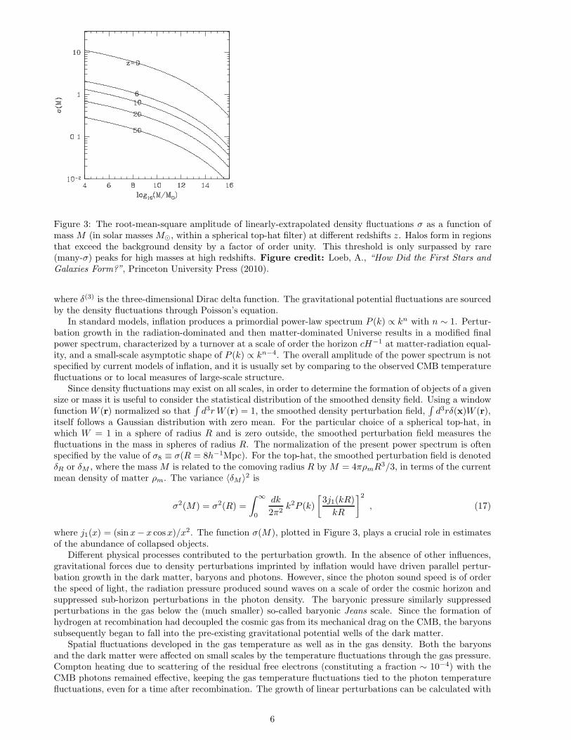
Figure 3: The root-mean-square amplitude of linearly-extrapolated density fluctuations σ as a function ofmass M (in solar masses M⊙, within a spherical top-hat filter) at different redshifts z. Halos form in regionsthat exceed the background density by a factor of order unity. This threshold is only surpassed by rare(many-σ) peaks for high masses at high redshifts. Figure credit: Loeb, A., “How Did the First Stars andGalaxies Form?”, Princeton University Press (2010).

where δ(3) is the three-dimensional Dirac delta function. The gravitational potential fluctuations are sourcedby the density fluctuations through Poisson’s equation.

In standard models, inflation produces a primordial power-law spectrum P (k) ∝ kn with n ∼ 1. Pertur-bation growth in the radiation-dominated and then matter-dominated Universe results in a modified finalpower spectrum, characterized by a turnover at a scale of order the horizon cH−1 at matter-radiation equal-ity, and a small-scale asymptotic shape of P (k) ∝ kn−4. The overall amplitude of the power spectrum is notspecified by current models of inflation, and it is usually set by comparing to the observed CMB temperaturefluctuations or to local measures of large-scale structure.

Since density fluctuations may exist on all scales, in order to determine the formation of objects of a givensize or mass it is useful to consider the statistical distribution of the smoothed density field. Using a windowfunction W (r) normalized so that

∫

d3r W (r) = 1, the smoothed density perturbation field,∫

d3rδ(x)W (r),itself follows a Gaussian distribution with zero mean. For the particular choice of a spherical top-hat, inwhich W = 1 in a sphere of radius R and is zero outside, the smoothed perturbation field measures thefluctuations in the mass in spheres of radius R. The normalization of the present power spectrum is oftenspecified by the value of σ8 ≡ σ(R = 8h−1Mpc). For the top-hat, the smoothed perturbation field is denotedδR or δM , where the mass M is related to the comoving radius R by M = 4πρmR3/3, in terms of the currentmean density of matter ρm. The variance 〈δM 〉2 is

σ2(M) = σ2(R) =

∫ ∞

0

dk

2π2k2P (k)

[

3j1(kR)

kR

]2

, (17)

where j1(x) = (sinx− x cosx)/x2. The function σ(M), plotted in Figure 3, plays a crucial role in estimatesof the abundance of collapsed objects.

Different physical processes contributed to the perturbation growth. In the absence of other influences,gravitational forces due to density perturbations imprinted by inflation would have driven parallel pertur-bation growth in the dark matter, baryons and photons. However, since the photon sound speed is of orderthe speed of light, the radiation pressure produced sound waves on a scale of order the cosmic horizon andsuppressed sub-horizon perturbations in the photon density. The baryonic pressure similarly suppressedperturbations in the gas below the (much smaller) so-called baryonic Jeans scale. Since the formation ofhydrogen at recombination had decoupled the cosmic gas from its mechanical drag on the CMB, the baryonssubsequently began to fall into the pre-existing gravitational potential wells of the dark matter.

Spatial fluctuations developed in the gas temperature as well as in the gas density. Both the baryonsand the dark matter were affected on small scales by the temperature fluctuations through the gas pressure.Compton heating due to scattering of the residual free electrons (constituting a fraction ∼ 10−4) with theCMB photons remained effective, keeping the gas temperature fluctuations tied to the photon temperaturefluctuations, even for a time after recombination. The growth of linear perturbations can be calculated with

6

the standard CMBFAST code (http://www.cmbfast.org), after a modification to account for the fact thatthe speed of sound of the gas also fluctuates spatially.

After recombination, two main drivers affect the baryon density and temperature fluctuations, namely,the thermalization with the CMB and the gravitational force that attracts the baryons to the dark matterpotential wells. The density perturbations in all species grow together on scales where gravity is unopposed,outside the horizon (i.e., at k < 0.01 Mpc−1 at z ∼ 1000). At z = 1200 the perturbations in the baryon-photon fluid oscillate as acoustic waves on scales of order the sound horizon (k ∼ 0.01 Mpc−1), whilesmaller-scale perturbations in both the photons and baryons are damped by photon diffusion and the dragof the diffusing photons on the baryons. On sufficiently small scales the power spectra of baryon density andtemperature roughly assume the shape of the dark matter fluctuations (except for the gas-pressure cutoff atthe very smallest scales), due to the effect of gravitational attraction on the baryon density and of the resultingadiabatic expansion on the gas temperature. After the mechanical coupling of the baryons to the photonsends at z ∼ 1000, the baryon density perturbations gradually grow towards the dark matter perturbationsbecause of gravity. Similarly, after the thermal coupling ends at z ∼ 200, the baryon temperature fluctuationsare driven by adiabatic expansion towards a value of 2/3 of the density fluctuations. By z = 200 the baryoninfall into the dark matter potentials is well advanced and adiabatic expansion is becoming increasinglyimportant in setting the baryon temperature.

2.2 Halo properties

The small density fluctuations evidenced in the CMB grow over time as described in the previous subsection,until the perturbation δ becomes of order unity, and the full non-linear gravitational problem must beconsidered. The dynamical collapse of a dark matter halo can be solved analytically only in cases of particularsymmetry. If we consider a region which is much smaller than the horizon cH−1, then the formation of ahalo can be formulated as a problem in Newtonian gravity, in some cases with minor corrections comingfrom General Relativity. The simplest case is that of spherical symmetry, with an initial (t = ti ≪ t0)top-hat of uniform overdensity δi inside a sphere of radius R. Although this model is restricted in its directapplicability, the results of spherical collapse have turned out to be surprisingly useful in understanding theproperties and distribution of halos in models based on cold dark matter.

The collapse of a spherical top-hat perturbation is described by the Newtonian equation (with a correctionfor the cosmological constant)

d2r

dt2= H2

0ΩΛ r − GM

r2, (18)

where r is the radius in a fixed (not comoving) coordinate frame, H0 is the present-day Hubble constant,M is the total mass enclosed within radius r, and the initial velocity field is given by the Hubble flowdr/dt = H(t)r. The enclosed δ grows initially as δL = δiD(t)/D(ti), in accordance with linear theory, buteventually δ grows above δL. If the mass shell at radius r is bound (i.e., if its total Newtonian energy isnegative) then it reaches a radius of maximum expansion and subsequently collapses. As demonstrated inthe previous section, at the moment when the top-hat collapses to a point, the overdensity predicted bylinear theory is δL = 1.686 in the Einstein-de Sitter model, with only a weak dependence on Ωm and ΩΛ.Thus a tophat collapses at redshift z if its linear overdensity extrapolated to the present day (also termedthe critical density of collapse) is

δcrit(z) =1.686

D(z), (19)

where we set D(z = 0) = 1.Even a slight violation of the exact symmetry of the initial perturbation can prevent the tophat from

collapsing to a point. Instead, the halo reaches a state of virial equilibrium by violent relaxation (phasemixing). Using the virial theorem U = −2K to relate the potential energy U to the kinetic energy Kin the final state (implying that the virial radius is half the turnaround radius - where the kinetic energyvanishes), the final overdensity relative to the critical density at the collapse redshift is ∆c = 18π2 ≃ 178 inthe Einstein-de Sitter model, modified in a Universe with Ωm + ΩΛ = 1 to the fitting formula

∆c = 18π2 + 82d − 39d2 , (20)

where d ≡ Ω zm − 1 is evaluated at the collapse redshift, so that

Ω zm =

Ωm(1 + z)3

Ωm(1 + z)3 + ΩΛ + Ωk(1 + z)2. (21)

7

Figure 4: Left panel: The mass fraction incorporated into dark matter halos per logarithmic bin of halo mass(M2dn/dM)/ρm, as a function of M at different redshifts z. Here ρm = Ωmρc is the present-day matterdensity, and n(M)dM is the comoving density of halos with masses between M and M +dM . The halo massdistribution was calculated based on an improved version of the Press-Schechter formalism for ellipsoidalcollapse [Sheth, R. K., & Tormen, G. Mon. Not. R. Astron. Soc. 329, 61 (2002)] that fits better numericalsimulations. Right panel: Number density of halos per logarithmic bin of halo mass, Mdn/dM (in units ofcomoving Mpc−3), at various redshifts. Figure credit: Loeb, A., “How Did the First Stars and GalaxiesForm?”, Princeton University Press (2010).

A halo of mass M collapsing at redshift z thus has a virial radius

rvir = 0.784

(

M

108 h−1 M⊙

)1/3 [

Ωm

Ω zm

∆c

18π2

]−1/3 (

1 + z

10

)−1

h−1 kpc , (22)

and a corresponding circular velocity,

Vc =

(

GM

rvir

)1/2

= 23.4

(

M

108 h−1 M⊙

)1/3 [

Ωm

Ω zm

∆c

18π2

]1/6 (

1 + z

10

)1/2

km s−1 . (23)

In these expressions we have assumed a present Hubble constant written in the form H0 = 100 h km s−1Mpc−1.We may also define a virial temperature

Tvir =µmpV

2c

2k= 1.98 × 104

( µ

0.6

)

(

M

108 h−1 M⊙

)2/3 [

Ωm

Ω zm

∆c

18π2

]1/3 (

1 + z

10

)

K , (24)

where µ is the mean molecular weight and mp is the proton mass. Note that the value of µ depends on theionization fraction of the gas; for a fully ionized primordial gas µ = 0.59, while a gas with ionized hydrogenbut only singly-ionized helium has µ = 0.61. The binding energy of the halo is approximately1

Eb =1

2

GM2

rvir= 5.45 × 1053

(

M

108 h−1 M⊙

)5/3 [

Ωm

Ω zm

∆c

18π2

]1/3 (

1 + z

10

)

h−1 erg . (25)

Note that the binding energy of the baryons is smaller by a factor equal to the baryon fraction Ωb/Ωm.Although spherical collapse captures some of the physics governing the formation of halos, structure

formation in cold dark matter models proceeds hierarchically. At early times, most of the dark matter isin low-mass halos, and these halos continuously accrete and merge to form high-mass halos (see Figure4). Numerical simulations of hierarchical halo formation indicate a roughly universal spherically-averageddensity profile for the resulting halos, though with considerable scatter among different halos. The typicalprofile has the form

ρ(r) =3H2

0

8πG(1 + z)3

Ωm

Ω zm

δc

cNx(1 + cNx)2, (26)

1The coefficient of 1/2 in equation (25) would be exact for a singular isothermal sphere with ρ(r) ∝ 1/r2.

8

where x = r/rvir, and the characteristic density δc is related to the concentration parameter cN by

δc =∆c

3

c3N

ln(1 + cN) − cN/(1 + cN). (27)

The concentration parameter itself depends on the halo mass M , at a given redshift z.

2.3 Formation of the first stars

Theoretical expectations for the properties of the first galaxies are based on the standard cosmological modeloutlined in the Introduction. The formation of the first bound objects marked the central milestone in thetransition from the initial simplicity (discussed in the previous subsection) to the present-day complexity.Stars and accreting black holes output copious radiation and also produced explosions and outflows thatbrought into the IGM chemical products from stellar nucleosynthesis and enhanced magnetic fields. However,the formation of the very first stars, in a universe that had not yet suffered such feedback, remains a well-specified problem for theorists.

Stars form when large amounts of matter collapse to high densities. However, the process can be stoppedif the pressure exerted by the hot intergalactic gas prevents outlying gas from falling into dark matterconcentrations. As the gas falls into a dark matter halo, it forms shocks due to converging supersonic flowsand in the process heats up and can only collapse further by first radiating its energy away. This restricts thisprocess of collapse to very large clumps of dark matter that are around 100 000 times the mass of the Sun.Inside these clumps, the shocked gas loses energy by emitting radiation from excited molecular hydrogenthat formed naturally within the primordial gas mixture of hydrogen and helium.

The first stars are expected to have been quite different from the stars that form today in the MilkyWay. The higher pressure within the primordial gas due to the presence of fewer cooling agents suggeststhat fragmentation only occurred into relatively large units, in which gravity could overcome the pressure.Due to the lack of carbon, nitrogen, and oxygen – elements that would normally dominate the nuclear energyproduction in modern massive stars – the first stars must have condensed to extremely high densities andtemperatures before nuclear reactions were able to heat the gas and balance gravity. These unusually massivestars produced high luminosities of UV photons, but their nuclear fuel was exhausted after 2–3 million years,resulting in a huge supernova or in collapse to a black hole. The heavy elements which were dispersed by thefirst supernovae in the surrounding gas, enabled the enriched gas to cool more effectively and fragment intolower mass stars. Simple calculations indicate that a carbon or oxygen enrichment of merely <10−3 of thesolar abundance is sufficient to allow solar mass stars to form. These second-generation “low-metallicity”stars are long-lived and could in principle be discovered in the halo of the Milky Way galaxy, providing fossilrecord of the earliest star formation episode in our cosmic environment.

Advances in computing power have made possible detailed numerical simulations of how the first starsformed. These simulations begin in the early universe, in which dark matter and gas are distributed uniformly,apart from tiny variations in density and temperature that are statistically distributed according to thepatterns observed in the CMB. In order to span the vast range of scales needed to simulate an individualstar within a cosmological context, the adopted codes zoom in repeatedly on the densest part of the firstcollapsing cloud that is found within the simulated volume. The simulation follows gravity, hydrodynamics,and chemical processes in the primordial gas, and resolves a scale that is > 10 orders of magnitudes smallerthan that of the simulated box. In state-of-the-art simulations, the resolved scale is approaching the scale ofthe proto-star. The simulations have established that the first stars formed within halos containing ∼ 105M⊙

in total mass, and indicate that the first stars most likely weighed tens to hundreds of solar masses each.To estimate when the first stars formed we must remember that the first 100 000 solar mass halos collapsed

in regions that happened to have a particularly high density enhancement very early on. There was initiallyonly a small abundance of such regions in the entire universe, so a simulation that is limited to a small volumeis unlikely to find such halos until much later. Simulating the entire universe is well beyond the capabilitiesof current simulations, but analytical models predict that the first observable star in the universe probablyformed 30 million years after the Big Bang, less than a quarter of one percent of the Universe’s total age of13.7 billion years.

Although stars were extremely rare at first, gravitational collapse increased the abundance of galactichalos and star formation sites with time (Figure 2). Radiation from the first stars is expected to haveeventually dissociated all the molecular hydrogen in the intergalactic medium, leading to the domination ofa second generation of larger galaxies where the gas cooled via radiative transitions in atomic hydrogen andhelium. Atomic cooling occurred in halos of mass above ∼ 108M⊙, in which the infalling gas was heatedabove 10,000 K and became ionized. The first galaxies to form through atomic cooling are expected tohave formed around redshift 45, and such galaxies were likely the main sites of star formation by the timereionization began in earnest. As the IGM was heated above 10,000 K by reionization, its pressure jumped

9

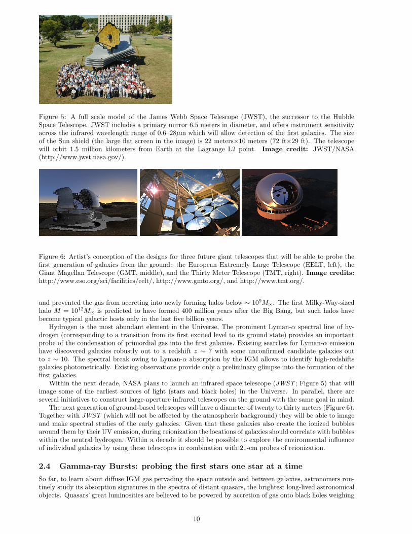
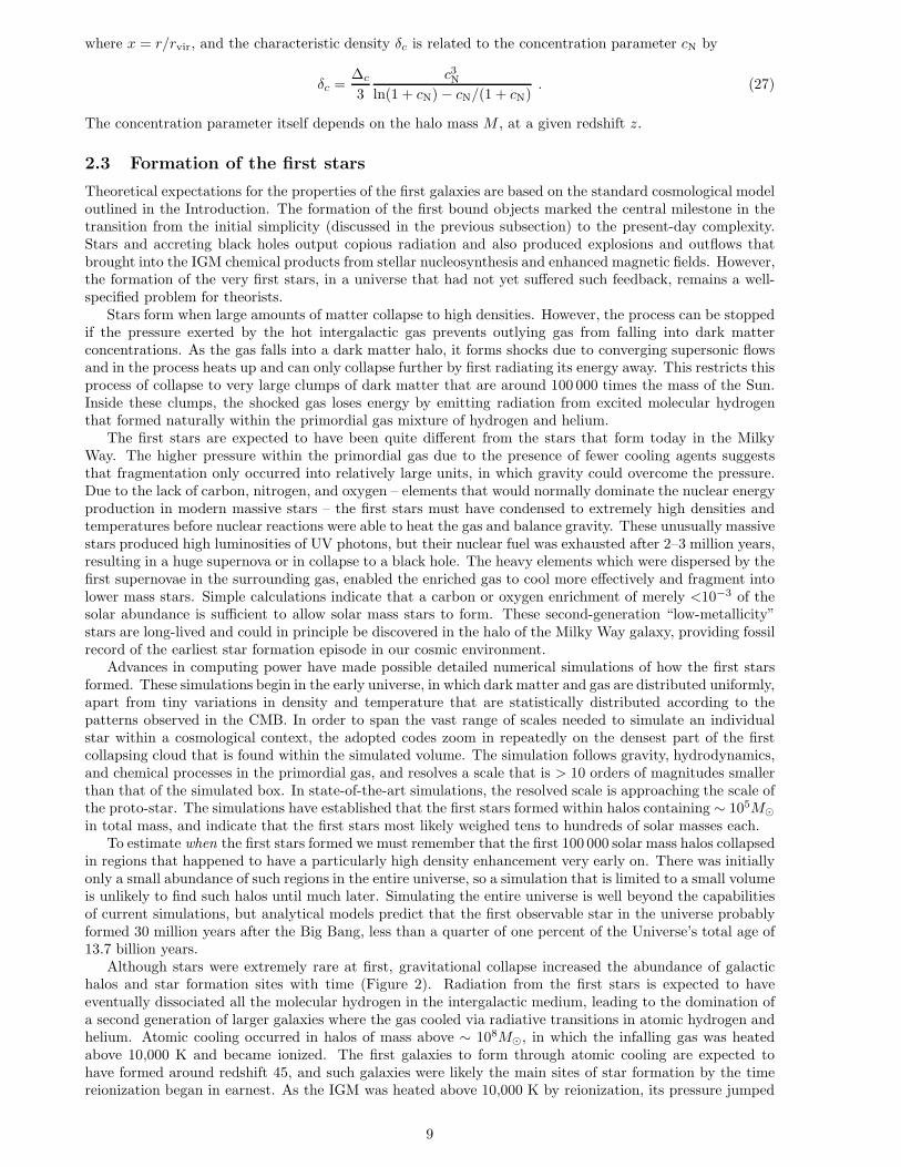
Figure 5: A full scale model of the James Webb Space Telescope (JWST), the successor to the HubbleSpace Telescope. JWST includes a primary mirror 6.5 meters in diameter, and offers instrument sensitivityacross the infrared wavelength range of 0.6–28µm which will allow detection of the first galaxies. The sizeof the Sun shield (the large flat screen in the image) is 22 meters×10 meters (72 ft×29 ft). The telescopewill orbit 1.5 million kilometers from Earth at the Lagrange L2 point. Image credit: JWST/NASA(http://www.jwst.nasa.gov/).

Figure 6: Artist’s conception of the designs for three future giant telescopes that will be able to probe thefirst generation of galaxies from the ground: the European Extremely Large Telescope (EELT, left), theGiant Magellan Telescope (GMT, middle), and the Thirty Meter Telescope (TMT, right). Image credits:http://www.eso.org/sci/facilities/eelt/, http://www.gmto.org/, and http://www.tmt.org/.

and prevented the gas from accreting into newly forming halos below ∼ 109M⊙. The first Milky-Way-sizedhalo M = 1012M⊙ is predicted to have formed 400 million years after the Big Bang, but such halos havebecome typical galactic hosts only in the last five billion years.

Hydrogen is the most abundant element in the Universe, The prominent Lyman-α spectral line of hy-drogen (corresponding to a transition from its first excited level to its ground state) provides an importantprobe of the condensation of primordial gas into the first galaxies. Existing searches for Lyman-α emissionhave discovered galaxies robustly out to a redshift z ∼ 7 with some unconfirmed candidate galaxies outto z ∼ 10. The spectral break owing to Lyman-α absorption by the IGM allows to identify high-redshiftsgalaxies photometrically. Existing observations provide only a preliminary glimpse into the formation of thefirst galaxies.

Within the next decade, NASA plans to launch an infrared space telescope (JWST ; Figure 5) that willimage some of the earliest sources of light (stars and black holes) in the Universe. In parallel, there areseveral initiatives to construct large-aperture infrared telescopes on the ground with the same goal in mind.

The next generation of ground-based telescopes will have a diameter of twenty to thirty meters (Figure 6).Together with JWST (which will not be affected by the atmospheric background) they will be able to imageand make spectral studies of the early galaxies. Given that these galaxies also create the ionized bubblesaround them by their UV emission, during reionization the locations of galaxies should correlate with bubbleswithin the neutral hydrogen. Within a decade it should be possible to explore the environmental influenceof individual galaxies by using these telescopes in combination with 21-cm probes of reionization.

2.4 Gamma-ray Bursts: probing the first stars one star at a time

So far, to learn about diffuse IGM gas pervading the space outside and between galaxies, astronomers rou-tinely study its absorption signatures in the spectra of distant quasars, the brightest long-lived astronomicalobjects. Quasars’ great luminosities are believed to be powered by accretion of gas onto black holes weighing

10

Figure 7: GRB afterglow flux as a function of time since the γ-ray trigger in the observer frame. The flux(solid curves) is calculated at the redshifted Lyman-α wavelength. The dotted curves show the planneddetection threshold for the James Webb Space Telescope (JWST), assuming a spectral resolution R = 5000with the near infrared spectrometer, a signal to noise ratio of 5 per spectral resolution element, and anexposure time equal to 20% of the time since the GRB explosion. Each set of curves shows a sequence ofredshifts, namely z = 5, 7, 9, 11, 13, and 15, respectively, from top to bottom. Figure credit: Barkana,R., & Loeb, A., Astrophys. J. 601, 64 (2004).

up to a few billion times the mass of the Sun that are situated in the centers of massive galaxies. As thesurrounding gas spirals in toward the black hole sink, the viscous dissipation of heat makes the gas glowbrightly into space, creating a luminous source visible from afar.

Over the past decade, an alternative population of bright sources at cosmological distances was discovered,the so-called afterglows of Gamma-Ray Bursts (GRBs). These events are characterized by a flash of high-energy (> 0.1 MeV) photons, typically lasting 0.1–100 seconds, which is followed by an afterglow of lower-energy photons over much longer timescales. The afterglow peaks at X-ray, UV, optical and eventuallyradio wavelengths on time scales of minutes, hours, days, and months, respectively. The central engines ofGRBs are believed to be associated with the compact remnants (neutron stars or stellar-mass black holes)of massive stars. Their high luminosities make them detectable out to the edge of the visible Universe.GRBs offer the opportunity to detect the most distant (and hence earliest) population of massive stars, theso-called Population III (or Pop III), one star at a time. In the hierarchical assembly process of halos thatare dominated by cold dark matter (CDM), the first galaxies should have had lower masses (and lower stellarluminosities) than their more recent counterparts. Consequently, the characteristic luminosity of galaxiesor quasars is expected to decline with increasing redshift. GRB afterglows, which already produce a peakflux comparable to that of quasars or starburst galaxies at z ∼ 1− 2, are therefore expected to outshine anycompeting source at the highest redshifts, when the first dwarf galaxies formed in the Universe.

GRBs, the electromagnetically-brightest explosions in the Universe, should be detectable out to redshiftsz > 10. High-redshift GRBs can be identified through infrared photometry, based on the Lyman-α breakinduced by absorption of their spectrum at wavelengths below 1.216 µm[(1+ z)/10]. Follow-up spectroscopyof high-redshift candidates can then be performed on a 10-meter-class telescope. GRB afterglows offer theopportunity to detect stars as well as to probe the metal enrichment level of the intervening IGM. Recently,the Swift satellite has detected a GRB originating at z ≃ 8.3, thus demonstrating the viability of GRBs asprobes of the early Universe.

Another advantage of GRBs is that the GRB afterglow flux at a given observed time lag after the γ-ray trigger is not expected to fade significantly with increasing redshift, since higher redshifts translateto earlier times in the source frame, during which the afterglow is intrinsically brighter. For standardafterglow lightcurves and spectra, the increase in the luminosity distance with redshift is compensated bythis cosmological time-stretching effect as shown in Figure 7.

GRB afterglows have smooth (broken power-law) continuum spectra unlike quasars which show strongspectral features (such as broad emission lines or the so-called “blue bump”) that complicate the extraction

11

of IGM absorption features. In particular, the extrapolation into the spectral regime marked by the IGMLyman-α absorption during the epoch of reionization is much more straightforward for the smooth UVspectra of GRB afterglows than for quasars with an underlying broad Lyman-α emission line. However,the interpretation may be complicated by the presence of damped Lyman-α absorption by dense neutralhydrogen in the immediate environment of the GRB within its host galaxy. Since GRBs originate from thedense environment of active star formation, such damped absorption is expected and indeed has been seen,including in the most distant GRB at z = 8.3.

2.5 Supermassive black holes

The fossil record in the present-day Universe indicates that every bulged galaxy hosts a supermassive blackhole (BH) at its center. This conclusion is derived from a variety of techniques which probe the dynamics ofstars and gas in galactic nuclei. The inferred BHs are dormant or faint most of the time, but occasionallyflash in a short burst of radiation that lasts for a small fraction of the age of the Universe. The short dutycycle accounts for the fact that bright quasars are much less abundant than their host galaxies, but it begsthe more fundamental question: why is the quasar activity so brief? A natural explanation is that quasarsare suicidal, namely the energy output from the BHs regulates their own growth.

Supermassive BHs make up a small fraction, < 10−3, of the total mass in their host galaxies, and sotheir direct dynamical impact is limited to the central star distribution where their gravitational influencedominates. Dynamical friction on the background stars keeps the BH close to the center. Random fluctu-ations in the distribution of stars induces a Brownian motion of the BH. This motion can be described bythe same Langevin equation that captures the motion of a massive dust particle as it responds to randomkicks from the much lighter molecules of air around it. The characteristic speed by which the BH wandersaround the center is small, ∼ (m⋆/MBH)1/2σ⋆, where m⋆ and MBH are the masses of a single star and theBH, respectively, and σ⋆ is the stellar velocity dispersion. Since the random force fluctuates on a dynamicaltime, the BH wanders across a region that is smaller by a factor of ∼ (m⋆/MBH)1/2 than the region traversedby the stars inducing the fluctuating force on it.

The dynamical insignificance of the BH on the global galactic scale is misleading. The gravitationalbinding energy per rest-mass energy of galaxies is of order ∼ (σ⋆/c)2 < 10−6. Since BH are relativisticobjects, the gravitational binding energy of material that feeds them amounts to a substantial fraction itsrest mass energy. Even if the BH mass amounts to a fraction as small as ∼ 10−4 of the baryonic mass in agalaxy, and only a percent of the accreted rest-mass energy is deposited into the gaseous environment of theBH, this slight deposition can unbind the entire gas reservoir of the host galaxy. This order-of-magnitudeestimate explains why quasars may be short lived. As soon as the central BH accretes large quantities ofgas so as to significantly increase its mass, it releases large amounts of energy and momentum that couldsuppress further accretion onto it. In short, the BH growth might be self-regulated.

The principle of self-regulation naturally leads to a correlation between the final BH mass, Mbh, andthe depth of the gravitational potential well to which the surrounding gas is confined. The latter can becharacterized by the velocity dispersion of the associated stars, ∼ σ2

⋆ . Indeed a correlation between Mbh

and σ4⋆ is observed in the present-day Universe. If quasars shine near their Eddington limit as suggested

by observations of low and high-redshift quasars, then a fraction of ∼ 5–10% of the energy released by thequasar over a galactic dynamical time needs to be captured in the surrounding galactic gas in order for theBH growth to be self-regulated. With this interpretation, the Mbh–σ⋆ relation reflects the limit introducedto the BH mass by self-regulation; deviations from this relation are inevitable during episodes of BH growthor as a result of mergers of galaxies that have no cold gas in them. A physical scatter around this upperenvelope could also result from variations in the efficiency by which the released BH energy couples to thesurrounding gas.

Various prescriptions for self-regulation were sketched in the literature. These involve either energy ormomentum-driven winds, with the latter type being a factor of ∼ vc/c less efficient. The quasar remainsactive during the dynamical time of the initial gas reservoir, ∼ 107 years, and fades afterwards due to thedilution of this reservoir. The BH growth may resume if the cold gas reservoir is replenished through a newmerger. Following early analytic work, extensive numerical simulations demonstrated that galaxy mergers doproduce the observed correlations between black hole mass and spheroid properties. Because of the limitedresolution near the galaxy nucleus, these simulations adopt a simple prescription for the accretion flow thatfeeds the black hole. The actual feedback in reality may depend crucially on the geometry of this flow andthe physical mechanism that couples the energy or momentum output of the quasar to the surrounding gas.

The inflow of cold gas towards galaxy centers during the growth phase of the BH would naturally beaccompanied by a burst of star formation. The fraction of gas that is not consumed by stars or ejectedby supernova-driven winds, will continue to feed the BH. It is therefore not surprising that quasar andstarburst activities co-exist in Ultra Luminous Infrared Galaxies, and that all quasars show broad metal

12

lines indicating pre-enrichment of the surrounding gas with heavy elements.The upper mass of galaxies may also be regulated by the energy output from quasar activity. This would

account for the fact that cooling flows are suppressed in present-day X-ray clusters, and that massive BHsand stars in galactic bulges were already formed at z ∼ 2. In the cores of cooling X-ray clusters, there isoften an active central BH that supplies sufficient energy to compensate for the cooling of the gas. Theprimary physical process by which this energy couples to the gas is still unknown.

The quasars discovered so far at z ∼ 6 mark the early growth of the most massive BHs and galacticspheroids. The BHs powering these bright quasars possess a mass of a few billion solar masses. A quasarradiating at its Eddington limiting luminosity, LE = 1.4 × 1047 erg s−1(Mbh/109M⊙), with a radiativeefficiency, ǫrad = LE/Mc2, for converting accreted mass into radiation, would grow exponentially in mass asa function of time t, Mbh = Mseed expt/tE from its initial seed mass Mseed, on a time scale, tE = 4.1 ×107 yr(ǫrad/0.1). Thus, the required growth time in units of the Hubble time thubble = 109 yr[(1 + z)/7]−3/2

istgrowth

thubble= 0.7

( ǫrad10%

)

(

1 + z

7

)3/2

ln

(

Mbh/109M⊙

Mseed/100M⊙

)

. (28)

The age of the Universe at z ∼ 6 provides just sufficient time to grow a BH with Mbh ∼ 109M⊙ out of astellar mass seed with ǫrad = 10%. The growth time is shorter for smaller radiative efficiencies or a higherseed mass.

2.6 The epoch of reionization

Given the understanding described above of how many galaxies formed at various times, the course ofreionization can be determined universe-wide by counting photons from all sources of light. Both starsand black holes contribute ionizing photons, but the early universe is dominated by small galaxies which inthe local universe have central black holes that are disproportionately small, and indeed quasars are rareabove redshift 6. Thus, stars most likely dominated the production of ionizing UV photons during thereionization epoch [although high-redshift galaxies should have also emitted X-rays from accreting blackholes and accelerated particles in collisionless shocks]. Since most stellar ionizing photons are only slightlymore energetic than the 13.6 eV ionization threshold of hydrogen, they are absorbed efficiently once theyreach a region with substantial neutral hydrogen). This makes the IGM during reionization a two-phasemedium characterized by highly ionized regions separated from neutral regions by sharp ionization fronts.

We can obtain a first estimate of the requirements of reionization by demanding one stellar ionizingphoton for each hydrogen atom in the IGM. If we conservatively assume that stars within the early galaxieswere similar to those observed locally, then each star produced ∼ 4000 ionizing photons per baryon. Starformation is observed today to be an inefficient process, but even if stars in galaxies formed out of only ∼ 10%of the available gas, it was still sufficient to accumulate a small fraction (of order 0.1%) of the total baryonicmass in the universe into galaxies in order to ionize the entire IGM. More accurate estimates of the actualrequired fraction account for the formation of some primordial stars (which were massive, efficient ionizers,as discussed above), and for recombinations of hydrogen atoms at high redshifts and in dense regions.

From studies of quasar absorption lines at z ∼ 6 we know that the IGM is highly ionized a billion yearsafter the big bang. There are hints, however, that some large neutral hydrogen regions persist at these earlytimes and so this suggests that we may not need to go to much higher redshifts to begin to see the epochof reionization. We now know that the universe could not have fully reionized earlier than an age of 300million years, since WMAP observed the effect of the freshly created plasma at reionization on the large-scale polarization anisotropies of the CMB and this limits the reionization redshift; an earlier reionization,when the universe was denser, would have created a stronger scattering signature that would be inconsistentwith the WMAP observations. In any case, the redshift at which reionization ended only constrains theoverall cosmic efficiency of ionizing photon production. In comparison, a detailed picture of reionization asit happens will teach us a great deal about the population of young galaxies that produced this cosmic phasetransition. A key point is that the spatial distribution of ionized bubbles is determined by clustered groupsof galaxies and not by individual galaxies. At such early times galaxies were strongly clustered even on verylarge scales (up to tens of Mpc), and these scales therefore dominate the structure of reionization. The basicidea is simple. At high redshift, galactic halos are rare and correspond to rare, high density peaks. As ananalogy, imagine searching on Earth for mountain peaks above 5000 meters. The 200 such peaks are not atall distributed uniformly but instead are found in a few distinct clusters on top of large mountain ranges.Given the large-scale boost provided by a mountain range, a small-scale crest need only provide a smalladditional rise in order to become a 5000 meter peak. The same crest, if it formed within a valley, would notcome anywhere near 5000 meters in total height. Similarly, in order to find the early galaxies, one must firstlocate a region with a large-scale density enhancement, and then galaxies will be found there in abundance.

13

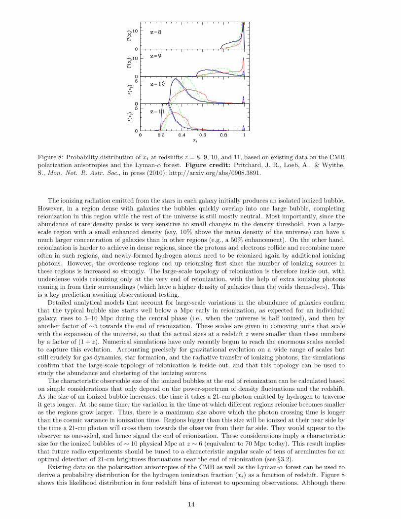
Figure 8: Probability distribution of xi at redshifts z = 8, 9, 10, and 11, based on existing data on the CMBpolarization anisotropies and the Lyman-α forest. Figure credit: Pritchard, J. R., Loeb, A.. & Wyithe,S., Mon. Not. R. Astr. Soc., in press (2010); http://arxiv.org/abs/0908.3891.

The ionizing radiation emitted from the stars in each galaxy initially produces an isolated ionized bubble.However, in a region dense with galaxies the bubbles quickly overlap into one large bubble, completingreionization in this region while the rest of the universe is still mostly neutral. Most importantly, since theabundance of rare density peaks is very sensitive to small changes in the density threshold, even a large-scale region with a small enhanced density (say, 10% above the mean density of the universe) can have amuch larger concentration of galaxies than in other regions (e.g., a 50% enhancement). On the other hand,reionization is harder to achieve in dense regions, since the protons and electrons collide and recombine moreoften in such regions, and newly-formed hydrogen atoms need to be reionized again by additional ionizingphotons. However, the overdense regions end up reionizing first since the number of ionizing sources inthese regions is increased so strongly. The large-scale topology of reionization is therefore inside out, withunderdense voids reionizing only at the very end of reionization, with the help of extra ionizing photonscoming in from their surroundings (which have a higher density of galaxies than the voids themselves). Thisis a key prediction awaiting observational testing.

Detailed analytical models that account for large-scale variations in the abundance of galaxies confirmthat the typical bubble size starts well below a Mpc early in reionization, as expected for an individualgalaxy, rises to 5–10 Mpc during the central phase (i.e., when the universe is half ionized), and then byanother factor of ∼5 towards the end of reionization. These scales are given in comoving units that scalewith the expansion of the universe, so that the actual sizes at a redshift z were smaller than these numbersby a factor of (1 + z). Numerical simulations have only recently begun to reach the enormous scales neededto capture this evolution. Accounting precisely for gravitational evolution on a wide range of scales butstill crudely for gas dynamics, star formation, and the radiative transfer of ionizing photons, the simulationsconfirm that the large-scale topology of reionization is inside out, and that this topology can be used tostudy the abundance and clustering of the ionizing sources.

The characteristic observable size of the ionized bubbles at the end of reionization can be calculated basedon simple considerations that only depend on the power-spectrum of density fluctuations and the redshift.As the size of an ionized bubble increases, the time it takes a 21-cm photon emitted by hydrogen to traverseit gets longer. At the same time, the variation in the time at which different regions reionize becomes smalleras the regions grow larger. Thus, there is a maximum size above which the photon crossing time is longerthan the cosmic variance in ionization time. Regions bigger than this size will be ionized at their near side bythe time a 21-cm photon will cross them towards the observer from their far side. They would appear to theobserver as one-sided, and hence signal the end of reionization. These considerations imply a characteristicsize for the ionized bubbles of ∼ 10 physical Mpc at z ∼ 6 (equivalent to 70 Mpc today). This result impliesthat future radio experiments should be tuned to a characteristic angular scale of tens of arcminutes for anoptimal detection of 21-cm brightness fluctuations near the end of reionization (see §3.2).

Existing data on the polarization anisotropies of the CMB as well as the Lyman-α forest can be used toderive a probability distribution for the hydrogen ionization fraction (xi) as a function of redshift. Figure 8shows this likelihood distribution in four redshift bins of interest to upcoming observations. Although there

14

is considerable uncertainty in xi at each redshift, it is evident from existing data that hydrogen is highlyionized by z = 8 (at least to xi > 0.8).

To produce one ionizing photon per baryon requires a minimum comoving density of Milky-Way (so-calledPopulation II) stars of,

ρ⋆ ≈ 1.7 × 106f−1esc M⊙ Mpc−3, (29)

or equivalently, a cosmological density parameter in stars of Ω⋆ ∼ 1.25 × 10−5f−1esc . More typically, the

threshold for reionization involves at least a few ionizing photons per proton (with the right-hand-side being∼ 10−6 cm−3), since the recombination time at the mean density is comparable to the age of the Universeat z ∼ 10.

For the local mass function of (Population II) stars at solar metallicity, the star formation rate per unitcomoving volume that is required for balancing recombinations in an already ionized IGM, is given by

ρ⋆ ≈ 2 × 10−3f−1escC

(

1 + z

10

)3

M⊙ yr−1 Mpc−3, (30)

where C = 〈n2e〉/〈nH〉2 is the volume-averaged clumpiness factor of the electron density up to some threshold

overdensity of gas which remains neutral. Current state-of-the-art surveys (HST WFC3/IR) are only sensitiveto the bright end of the luminosity function of galaxies at z > 6 and hence provide a lower limit on theproduction rate of ionizing photons during reionization.

2.7 Post-reionization suppression of low-mass galaxies

After the ionized bubbles overlapped in each region, the ionizing background increased sharply, and the IGMwas heated by the ionizing radiation to a temperature TIGM > 104 K. Due to the substantial increase in theIGM pressure, the smallest mass scale into which the cosmic gas could fragment, the so-called Jeans mass,increased dramatically, changing the minimum mass of forming galaxies.

Gas infall depends sensitively on the Jeans mass. When a halo more massive than the Jeans massbegins to form, the gravity of its dark matter overcomes the gas pressure. Even in halos below the Jeansmass, although the gas is initially held up by pressure, once the dark matter collapses its increased gravitypulls in some gas. Thus, the Jeans mass is generally higher than the actual limiting mass for accretion.Before reionization, the IGM is cold and neutral, and the Jeans mass plays a secondary role in limitinggalaxy formation compared to cooling. After reionization, the Jeans mass is increased by several orders ofmagnitude due to the photoionization heating of the IGM, and hence begins to play a dominant role inlimiting the formation of stars. Gas infall in a reionized and heated Universe has been investigated in anumber of numerical simulations. Three dimensional numerical simulations found a significant suppressionof gas infall in even larger halos (Vc ∼ 75 km s−1), but this was mostly due to a suppression of late infall atz<2.

When a volume of the IGM is ionized by stars, the gas is heated to a temperature TIGM ∼ 104 K. Ifquasars dominate the UV background at reionization, their harder photon spectrum leads to TIGM > 2×104

K. Including the effects of dark matter, a given temperature results in a linear Jeans mass corresponding toa halo circular velocity of

VJ ≈ 80

(

TIGM

1.5 × 104K

)1/2

km s−1. (31)

In halos with a circular velocity well above VJ , the gas fraction in infalling gas equals the universal meanof Ωb/Ωm, but gas infall is suppressed in smaller halos. A simple estimate of the limiting circular velocity,below which halos have essentially no gas infall, is obtained by substituting the virial overdensity for themean density in the definition of the Jeans mass. The resulting estimate is

Vlim = 34

(

TIGM

1.5 × 104K

)1/2

km s−1. (32)

This value is in rough agreement with the numerical simulations mentioned before.Although the Jeans mass is closely related to the rate of gas infall at a given time, it does not directly

yield the total gas residing in halos at a given time. The latter quantity depends on the entire history of gasaccretion onto halos, as well as on the merger histories of halos, and an accurate description must involve atime-averaged Jeans mass. The gas content of halos in simulations is well fit by an expression which dependson the filtering mass, a particular time-averaged Jeans mass.

The reionization process was not perfectly synchronized throughout the Universe. Large-scale regionswith a higher density than the mean tended to form galaxies first and reionized earlier than underdenseregions. The suppression of low-mass galaxies by reionization is therefore modulated by the fluctuations

15

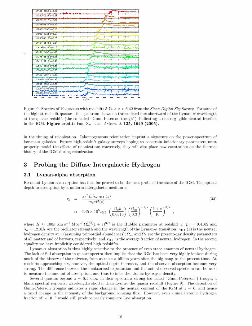
Figure 9: Spectra of 19 quasars with redshifts 5.74 < z < 6.42 from the Sloan Digital Sky Survey. For some ofthe highest-redshift quasars, the spectrum shows no transmitted flux shortward of the Lyman-α wavelengthat the quasar redshift (the so-called “Gunn-Peterson trough”), indicating a non-negligible neutral fractionin the IGM. Figure credit: Fan, X., et al. Astron. J. 125, 1649 (2005).

in the timing of reionization. Inhomogeneous reionization imprint a signature on the power-spectrum oflow-mass galaxies. Future high-redshift galaxy surveys hoping to constrain inflationary parameters mustproperly model the effects of reionization; conversely, they will also place new constraints on the thermalhistory of the IGM during reionization.

3 Probing the Diffuse Intergalactic Hydrogen

3.1 Lyman-alpha absorption

Resonant Lyman-α absorption has thus far proved to be the best probe of the state of the IGM. The opticaldepth to absorption by a uniform intergalactic medium is

τs =πe2fαλαnH I (z)

mecH(z)(33)

≈ 6.45 × 105xH I

(

Ωbh

0.0315

) (

Ωm

0.3

)−1/2 (

1 + z

10

)3/2

,

where H ≈ 100h km s−1 Mpc−1Ω1/2m (1 + z)3/2 is the Hubble parameter at redshift z; fα = 0.4162 and

λα = 1216A are the oscillator strength and the wavelength of the Lyman-α transition; nH I (z) is the neutralhydrogen density at z (assuming primordial abundances); Ωm and Ωb are the present-day density parametersof all matter and of baryons, respectively; and xH I is the average fraction of neutral hydrogen. In the secondequality we have implicitly considered high redshifts.

Lyman-α absorption is thus highly sensitive to the presence of even trace amounts of neutral hydrogen.The lack of full absorption in quasar spectra then implies that the IGM has been very highly ionized duringmuch of the history of the universe, from at most a billion years after the big bang to the present time. Atredshifts approaching six, however, the optical depth increases, and the observed absorption becomes verystrong. The difference between the unabsorbed expectation and the actual observed spectrum can be usedto measure the amount of absorption, and thus to infer the atomic hydrogen density.

Several quasars beyond z ∼ 6.1 show in their spectra a strong (so-called “Gunn-Peterson”) trough, ablank spectral region at wavelengths shorter than Lyα at the quasar redshift (Figure 9). The detection ofGunn-Peterson troughs indicates a rapid change in the neutral content of the IGM at z ∼ 6, and hencea rapid change in the intensity of the background ionizing flux. However, even a small atomic hydrogenfraction of ∼ 10−3 would still produce nearly complete Lyα absorption.

16

While only resonant Lyα absorption is important at moderate redshifts, the damping wing of the Lyα lineplays a significant role when neutral fractions of order unity are considered at z > 6. The scattering cross-section of the Lyα resonance line by neutral hydrogen is given by

σα(ν) =3λ2

αΛ2α

8π

(ν/να)4

4π2(ν − να)2 + (Λ2α/4)(ν/να)6

, (34)

where Λα = (8π2e2fα/3mecλ2α) = 6.25 × 108 s−1 is the Lyα (2p → 1s) decay rate, fα = 0.4162 is the

oscillator strength, and λα = 1216A and να = (c/λα) = 2.47× 1015 Hz are the wavelength and frequency ofthe Lyα line. The term in the numerator is responsible for the classical Rayleigh scattering.

Although reionization is an inhomogeneous process, we consider here a simple illustrative case of instan-taneous reionization. Consider a source at a redshift zs beyond the redshift of reionization, zreion, and thecorresponding scattering optical depth of a uniform, neutral IGM of hydrogen density nH,0(1 + z)3 betweenthe source and the reionization redshift. The optical depth is a function of the observed wavelength λobs,

τ(λobs) =

∫ zs

zreion

dzcdt

dznH,0(1 + z)3σα [νobs(1 + z)] , (35)

where νobs = c/λobs and for a flat Universe with (Ωm + ΩΛ) = 1,

dt

dz= [(1 + z)H(z)]−1 = H−1

0 ×[

Ωm(1 + z)5 + ΩΛ(1 + z)2]−1/2

. (36)

At wavelengths longer than Lyα at the source, the optical depth obtains a small value; these photonsredshift away from the line center along its red wing and never resonate with the line core on their wayto the observer. Considering only the regime in which |ν − να| ≫ Λα, we may ignore the second termin the denominator of equation (34). This leads to an analytical result for the red damping wing of theGunn-Peterson trough,

τ(λobs) = τs

(

Λ

4π2να

)

λ3/2obs

[

I(λ−1obs) − I([(1 + zreion)/(1 + zs)]λ

−1obs)

]

, (37)

an expression valid for λobs ≥ 1, where τs is given in equation (33), and we also define

λobs ≡λobs

(1 + zs)λα(38)

and

I(x) ≡ x9/2

1 − x+

9

7x7/2 +

9

5x5/2 + 3x3/2 + 9x1/2 − 9

2ln

[

1 + x1/2

1 − x1/2

]

. (39)

3.2 21-cm absorption or emission

3.2.1 The spin temperature of the 21-cm transition of hydrogen

The ground state of hydrogen exhibits hyperfine splitting owing to the possibility of two relative alignmentsof the spins of the proton and the electron. The state with parallel spins (the triplet state) has a slightlyhigher energy than the state with anti-parallel spins (the singlet state). The 21-cm line associated with thespin-flip transition from the triplet to the singlet state is often used to detect neutral hydrogen in the localuniverse. At high redshift, the occurrence of a neutral pre-reionization IGM offers the prospect of detectingthe first sources of radiation and probing the reionization era by mapping the 21-cm emission from neutralregions. While its energy density is estimated to be only a 1% correction to that of the CMB, the redshifted21-cm emission should display angular structure as well as frequency structure due to inhomogeneities in thegas density field, hydrogen ionized fraction, and spin temperature. Indeed, a full mapping of the distributionof H I as a function of redshift is possible in principle.

The basic physics of the hydrogen spin transition is determined as follows. The ground-state hyperfinelevels of hydrogen tend to thermalize with the CMB background, making the IGM unobservable. If otherprocesses shift the hyperfine level populations away from thermal equilibrium, then the gas becomes ob-servable against the CMB in emission or in absorption. The relative occupancy of the spin levels is usuallydescribed in terms of the hydrogen spin temperature TS , defined by

n1

n0= 3 exp

−T∗

TS

, (40)

17

where n0 and n1 refer respectively to the singlet and triplet hyperfine levels in the atomic ground state (n =1), and T∗ = 0.068 K is defined by kBT∗ = E21, where the energy of the 21 cm transition is E21 = 5.9×10−6

eV, corresponding to a frequency of 1420 MHz. In the presence of the CMB alone, the spin states reachthermal equilibrium with TS = TCMB = 2.725(1 + z) K on a time-scale of T∗/(TCMBA10) ≃ 3× 105(1 + z)−1

yr, where A10 = 2.87 × 10−15 s−1 is the spontaneous decay rate of the hyperfine transition. This time-scaleis much shorter than the age of the universe at all redshifts after cosmological recombination.

The IGM is observable when the kinetic temperature Tk of the gas differs from TCMB and an effectivemechanism couples TS to Tk. Collisional de-excitation of the triplet level dominates at very high redshift,when the gas density (and thus the collision rate) is still high, but once a significant galaxy populationforms in the universe, the spin temperature is affected also by an indirect mechanism that acts through thescattering of Lyman-α photons. Continuum UV photons produced by early radiation sources redshift by theHubble expansion into the local Lyman-α line at a lower redshift. These photons mix the spin states via theWouthuysen-Field process whereby an atom initially in the n = 1 state absorbs a Lyman-α photon, and thespontaneous decay which returns it from n = 2 to n = 1 can result in a final spin state which is different fromthe initial one. Since the neutral IGM is highly opaque to resonant scattering, and the Lyman-α photonsreceive Doppler kicks in each scattering, the shape of the radiation spectrum near Lyman-α is determinedby Tk, and the resulting spin temperature (assuming TS ≫ T∗) is then a weighted average of Tk and TCMB:

TS =TCMBTk(1 + xtot)

Tk + TCMBxtot, (41)

where xtot = xα + xc is the sum of the radiative and collisional threshold parameters. These parameters are

xα =P10T⋆

A10TCMB, (42)

and

xc =4κ1−0(Tk)nHT⋆

3A10TCMB, (43)

where P10 is the indirect de-excitation rate of the triplet n = 1 state via the Wouthuysen-Field process,related to the total scattering rate Pα of Lyman-α photons by P10 = 4Pα/27. Also, the atomic coefficientκ1−0(Tk) is tabulated as a function of Tk. The coupling of the spin temperature to the gas temperaturebecomes substantial when xtot > 1; in particular, xα = 1 defines the thermalization rate of Pα:

Pth ≡ 27A10TCMB

4T∗

≃ 7.6 × 10−12

(

1 + z

10

)

s−1 . (44)

A patch of neutral hydrogen at the mean density and with a uniform TS produces (after correcting forstimulated emission) an optical depth at a present-day (observed) wavelength of 21(1 + z) cm,

τ(z) = 9.0 × 10−3

(

TCMB

TS

) (

Ωbh

0.03

)(

Ωm

0.3

)−1/2 (

1 + z

10

)1/2

, (45)

assuming a high redshift z ≫ 1. The observed spectral intensity Iν relative to the CMB at a frequency νis measured by radio astronomers as an effective brightness temperature Tb of blackbody emission at thisfrequency, defined using the Rayleigh-Jeans limit of the Planck radiation formula: Iν ≡ 2kBTbν

2/c2.The brightness temperature through the IGM is Tb = TCMBe−τ +TS(1−e−τ ), so the observed differential

antenna temperature of this region relative to the CMB is

Tb = (1 + z)−1(TS − TCMB)(1 − e−τ )

≃ 28 mK

(

Ωbh

0.033

) (

Ωm

0.27

)−1/2 (

1 + z

10

)1/2 (

TS − TCMB

TS

)

, (46)

where τ ≪ 1 is assumed and Tb has been redshifted to redshift zero. Note that the combination that appearsin Tb is

TS − TCMB

TS=

xtot

1 + xtot

(

1 − TCMB

Tk

)

. (47)

In overdense regions, the observed Tb is proportional to the overdensity, and in partially ionized regions Tb

is proportional to the neutral fraction. Also, if TS ≫ TCMB then the IGM is observed in emission at a levelthat is independent of TS . On the other hand, if TS ≪ TCMB then the IGM is observed in absorption at alevel that is enhanced by a factor of TCMB/TS. As a result, a number of cosmic events are expected to leaveobservable signatures in the redshifted 21-cm line, as discussed below in further detail.

18

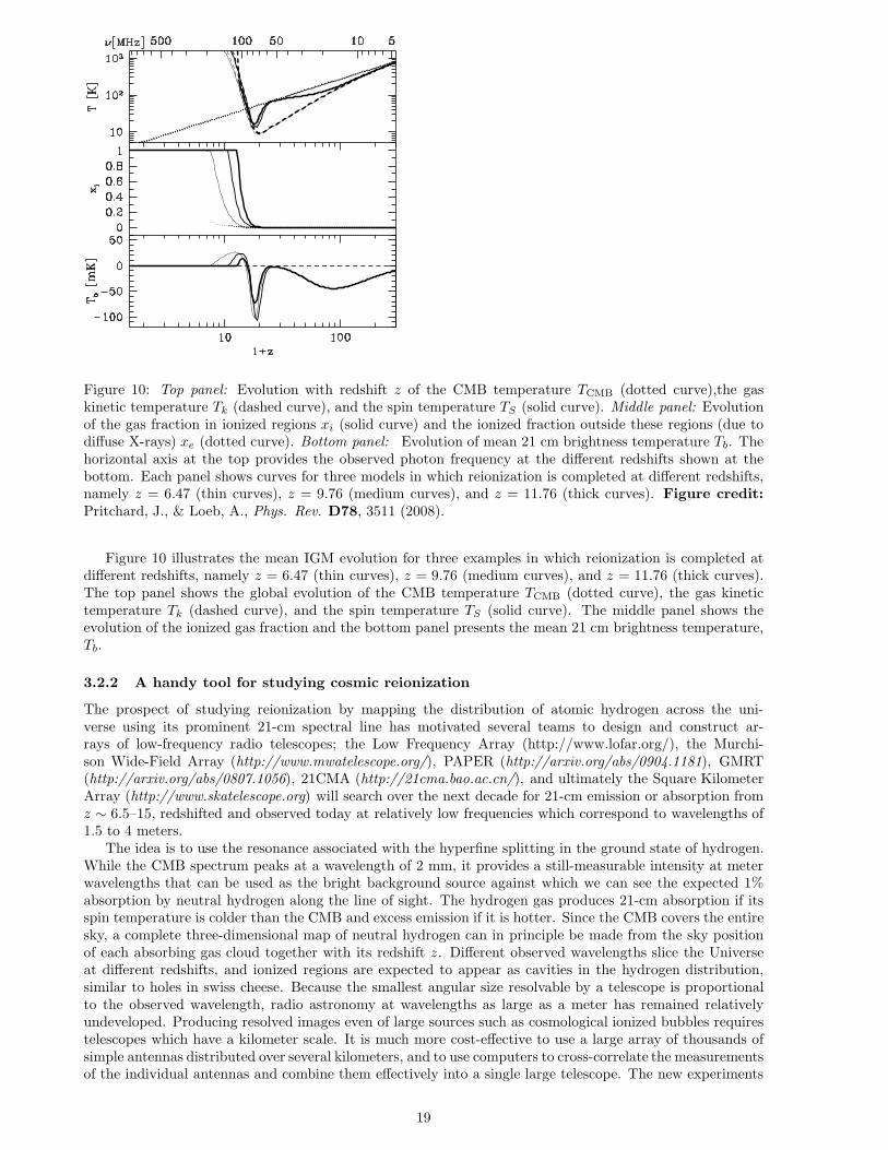
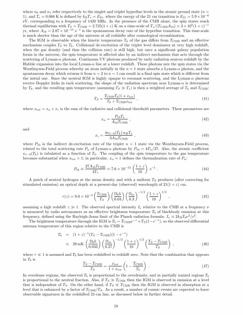
Figure 10: Top panel: Evolution with redshift z of the CMB temperature TCMB (dotted curve),the gaskinetic temperature Tk (dashed curve), and the spin temperature TS (solid curve). Middle panel: Evolutionof the gas fraction in ionized regions xi (solid curve) and the ionized fraction outside these regions (due todiffuse X-rays) xe (dotted curve). Bottom panel: Evolution of mean 21 cm brightness temperature Tb. Thehorizontal axis at the top provides the observed photon frequency at the different redshifts shown at thebottom. Each panel shows curves for three models in which reionization is completed at different redshifts,namely z = 6.47 (thin curves), z = 9.76 (medium curves), and z = 11.76 (thick curves). Figure credit:Pritchard, J., & Loeb, A., Phys. Rev. D78, 3511 (2008).

Figure 10 illustrates the mean IGM evolution for three examples in which reionization is completed atdifferent redshifts, namely z = 6.47 (thin curves), z = 9.76 (medium curves), and z = 11.76 (thick curves).The top panel shows the global evolution of the CMB temperature TCMB (dotted curve), the gas kinetictemperature Tk (dashed curve), and the spin temperature TS (solid curve). The middle panel shows theevolution of the ionized gas fraction and the bottom panel presents the mean 21 cm brightness temperature,Tb.

3.2.2 A handy tool for studying cosmic reionization

The prospect of studying reionization by mapping the distribution of atomic hydrogen across the uni-verse using its prominent 21-cm spectral line has motivated several teams to design and construct ar-rays of low-frequency radio telescopes; the Low Frequency Array (http://www.lofar.org/), the Murchi-son Wide-Field Array (http://www.mwatelescope.org/), PAPER (http://arxiv.org/abs/0904.1181), GMRT(http://arxiv.org/abs/0807.1056), 21CMA (http://21cma.bao.ac.cn/), and ultimately the Square KilometerArray (http://www.skatelescope.org) will search over the next decade for 21-cm emission or absorption fromz ∼ 6.5–15, redshifted and observed today at relatively low frequencies which correspond to wavelengths of1.5 to 4 meters.

The idea is to use the resonance associated with the hyperfine splitting in the ground state of hydrogen.While the CMB spectrum peaks at a wavelength of 2 mm, it provides a still-measurable intensity at meterwavelengths that can be used as the bright background source against which we can see the expected 1%absorption by neutral hydrogen along the line of sight. The hydrogen gas produces 21-cm absorption if itsspin temperature is colder than the CMB and excess emission if it is hotter. Since the CMB covers the entiresky, a complete three-dimensional map of neutral hydrogen can in principle be made from the sky positionof each absorbing gas cloud together with its redshift z. Different observed wavelengths slice the Universeat different redshifts, and ionized regions are expected to appear as cavities in the hydrogen distribution,similar to holes in swiss cheese. Because the smallest angular size resolvable by a telescope is proportionalto the observed wavelength, radio astronomy at wavelengths as large as a meter has remained relativelyundeveloped. Producing resolved images even of large sources such as cosmological ionized bubbles requirestelescopes which have a kilometer scale. It is much more cost-effective to use a large array of thousands ofsimple antennas distributed over several kilometers, and to use computers to cross-correlate the measurementsof the individual antennas and combine them effectively into a single large telescope. The new experiments

19

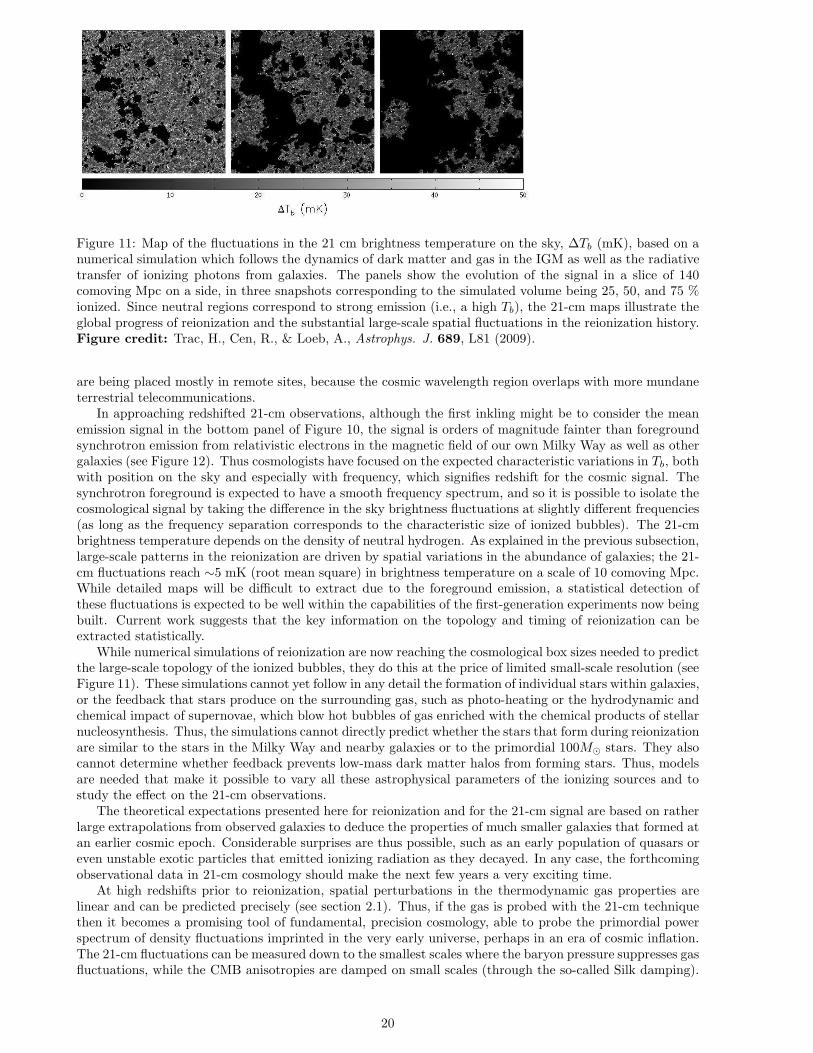
Figure 11: Map of the fluctuations in the 21 cm brightness temperature on the sky, ∆Tb (mK), based on anumerical simulation which follows the dynamics of dark matter and gas in the IGM as well as the radiativetransfer of ionizing photons from galaxies. The panels show the evolution of the signal in a slice of 140comoving Mpc on a side, in three snapshots corresponding to the simulated volume being 25, 50, and 75 %ionized. Since neutral regions correspond to strong emission (i.e., a high Tb), the 21-cm maps illustrate theglobal progress of reionization and the substantial large-scale spatial fluctuations in the reionization history.Figure credit: Trac, H., Cen, R., & Loeb, A., Astrophys. J. 689, L81 (2009).

are being placed mostly in remote sites, because the cosmic wavelength region overlaps with more mundaneterrestrial telecommunications.

In approaching redshifted 21-cm observations, although the first inkling might be to consider the meanemission signal in the bottom panel of Figure 10, the signal is orders of magnitude fainter than foregroundsynchrotron emission from relativistic electrons in the magnetic field of our own Milky Way as well as othergalaxies (see Figure 12). Thus cosmologists have focused on the expected characteristic variations in Tb, bothwith position on the sky and especially with frequency, which signifies redshift for the cosmic signal. Thesynchrotron foreground is expected to have a smooth frequency spectrum, and so it is possible to isolate thecosmological signal by taking the difference in the sky brightness fluctuations at slightly different frequencies(as long as the frequency separation corresponds to the characteristic size of ionized bubbles). The 21-cmbrightness temperature depends on the density of neutral hydrogen. As explained in the previous subsection,large-scale patterns in the reionization are driven by spatial variations in the abundance of galaxies; the 21-cm fluctuations reach ∼5 mK (root mean square) in brightness temperature on a scale of 10 comoving Mpc.While detailed maps will be difficult to extract due to the foreground emission, a statistical detection ofthese fluctuations is expected to be well within the capabilities of the first-generation experiments now beingbuilt. Current work suggests that the key information on the topology and timing of reionization can beextracted statistically.

While numerical simulations of reionization are now reaching the cosmological box sizes needed to predictthe large-scale topology of the ionized bubbles, they do this at the price of limited small-scale resolution (seeFigure 11). These simulations cannot yet follow in any detail the formation of individual stars within galaxies,or the feedback that stars produce on the surrounding gas, such as photo-heating or the hydrodynamic andchemical impact of supernovae, which blow hot bubbles of gas enriched with the chemical products of stellarnucleosynthesis. Thus, the simulations cannot directly predict whether the stars that form during reionizationare similar to the stars in the Milky Way and nearby galaxies or to the primordial 100M⊙ stars. They alsocannot determine whether feedback prevents low-mass dark matter halos from forming stars. Thus, modelsare needed that make it possible to vary all these astrophysical parameters of the ionizing sources and tostudy the effect on the 21-cm observations.

The theoretical expectations presented here for reionization and for the 21-cm signal are based on ratherlarge extrapolations from observed galaxies to deduce the properties of much smaller galaxies that formed atan earlier cosmic epoch. Considerable surprises are thus possible, such as an early population of quasars oreven unstable exotic particles that emitted ionizing radiation as they decayed. In any case, the forthcomingobservational data in 21-cm cosmology should make the next few years a very exciting time.

At high redshifts prior to reionization, spatial perturbations in the thermodynamic gas properties arelinear and can be predicted precisely (see section 2.1). Thus, if the gas is probed with the 21-cm techniquethen it becomes a promising tool of fundamental, precision cosmology, able to probe the primordial powerspectrum of density fluctuations imprinted in the very early universe, perhaps in an era of cosmic inflation.The 21-cm fluctuations can be measured down to the smallest scales where the baryon pressure suppresses gasfluctuations, while the CMB anisotropies are damped on small scales (through the so-called Silk damping).

20

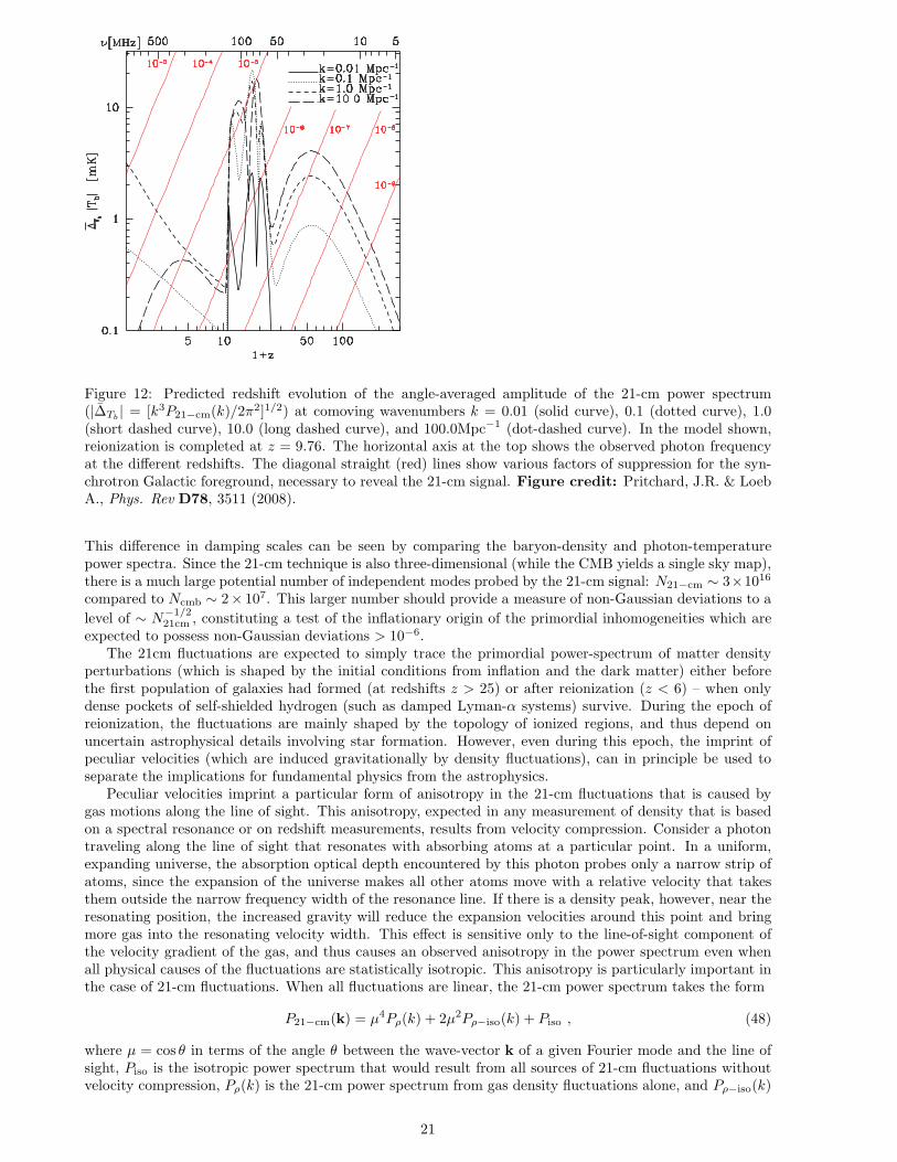
Figure 12: Predicted redshift evolution of the angle-averaged amplitude of the 21-cm power spectrum(|∆Tb

| = [k3P21−cm(k)/2π2]1/2) at comoving wavenumbers k = 0.01 (solid curve), 0.1 (dotted curve), 1.0(short dashed curve), 10.0 (long dashed curve), and 100.0Mpc−1 (dot-dashed curve). In the model shown,reionization is completed at z = 9.76. The horizontal axis at the top shows the observed photon frequencyat the different redshifts. The diagonal straight (red) lines show various factors of suppression for the syn-chrotron Galactic foreground, necessary to reveal the 21-cm signal. Figure credit: Pritchard, J.R. & LoebA., Phys. Rev D78, 3511 (2008).

This difference in damping scales can be seen by comparing the baryon-density and photon-temperaturepower spectra. Since the 21-cm technique is also three-dimensional (while the CMB yields a single sky map),there is a much large potential number of independent modes probed by the 21-cm signal: N21−cm ∼ 3×1016

compared to Ncmb ∼ 2× 107. This larger number should provide a measure of non-Gaussian deviations to a

level of ∼ N−1/221cm , constituting a test of the inflationary origin of the primordial inhomogeneities which are

expected to possess non-Gaussian deviations > 10−6.The 21cm fluctuations are expected to simply trace the primordial power-spectrum of matter density

perturbations (which is shaped by the initial conditions from inflation and the dark matter) either beforethe first population of galaxies had formed (at redshifts z > 25) or after reionization (z < 6) – when onlydense pockets of self-shielded hydrogen (such as damped Lyman-α systems) survive. During the epoch ofreionization, the fluctuations are mainly shaped by the topology of ionized regions, and thus depend onuncertain astrophysical details involving star formation. However, even during this epoch, the imprint ofpeculiar velocities (which are induced gravitationally by density fluctuations), can in principle be used toseparate the implications for fundamental physics from the astrophysics.

Peculiar velocities imprint a particular form of anisotropy in the 21-cm fluctuations that is caused bygas motions along the line of sight. This anisotropy, expected in any measurement of density that is basedon a spectral resonance or on redshift measurements, results from velocity compression. Consider a photontraveling along the line of sight that resonates with absorbing atoms at a particular point. In a uniform,expanding universe, the absorption optical depth encountered by this photon probes only a narrow strip ofatoms, since the expansion of the universe makes all other atoms move with a relative velocity that takesthem outside the narrow frequency width of the resonance line. If there is a density peak, however, near theresonating position, the increased gravity will reduce the expansion velocities around this point and bringmore gas into the resonating velocity width. This effect is sensitive only to the line-of-sight component ofthe velocity gradient of the gas, and thus causes an observed anisotropy in the power spectrum even whenall physical causes of the fluctuations are statistically isotropic. This anisotropy is particularly important inthe case of 21-cm fluctuations. When all fluctuations are linear, the 21-cm power spectrum takes the form

P21−cm(k) = µ4Pρ(k) + 2µ2Pρ−iso(k) + Piso , (48)

where µ = cos θ in terms of the angle θ between the wave-vector k of a given Fourier mode and the line ofsight, Piso is the isotropic power spectrum that would result from all sources of 21-cm fluctuations withoutvelocity compression, Pρ(k) is the 21-cm power spectrum from gas density fluctuations alone, and Pρ−iso(k)

21

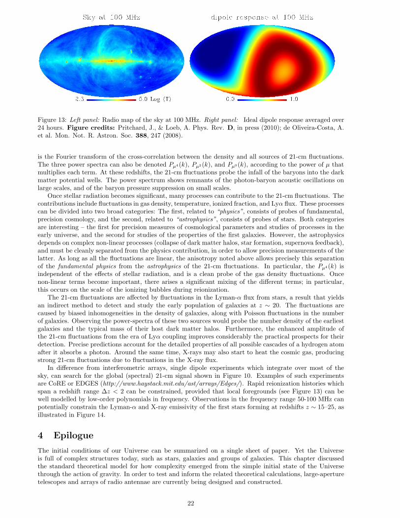
Figure 13: Left panel: Radio map of the sky at 100 MHz. Right panel: Ideal dipole response averaged over24 hours. Figure credits: Pritchard, J., & Loeb, A. Phys. Rev. D, in press (2010); de Oliveira-Costa, A.et al. Mon. Not. R. Astron. Soc. 388, 247 (2008).

is the Fourier transform of the cross-correlation between the density and all sources of 21-cm fluctuations.The three power spectra can also be denoted Pµ4(k), Pµ2(k), and Pµ0(k), according to the power of µ thatmultiplies each term. At these redshifts, the 21-cm fluctuations probe the infall of the baryons into the darkmatter potential wells. The power spectrum shows remnants of the photon-baryon acoustic oscillations onlarge scales, and of the baryon pressure suppression on small scales.

Once stellar radiation becomes significant, many processes can contribute to the 21-cm fluctuations. Thecontributions include fluctuations in gas density, temperature, ionized fraction, and Lyα flux. These processescan be divided into two broad categories: The first, related to “physics”, consists of probes of fundamental,precision cosmology, and the second, related to “astrophysics”, consists of probes of stars. Both categoriesare interesting – the first for precision measures of cosmological parameters and studies of processes in theearly universe, and the second for studies of the properties of the first galaxies. However, the astrophysicsdepends on complex non-linear processes (collapse of dark matter halos, star formation, supernova feedback),and must be cleanly separated from the physics contribution, in order to allow precision measurements of thelatter. As long as all the fluctuations are linear, the anisotropy noted above allows precisely this separationof the fundamental physics from the astrophysics of the 21-cm fluctuations. In particular, the Pµ4(k) isindependent of the effects of stellar radiation, and is a clean probe of the gas density fluctuations. Oncenon-linear terms become important, there arises a significant mixing of the different terms; in particular,this occurs on the scale of the ionizing bubbles during reionization.

The 21-cm fluctuations are affected by fluctuations in the Lyman-α flux from stars, a result that yieldsan indirect method to detect and study the early population of galaxies at z ∼ 20. The fluctuations arecaused by biased inhomogeneities in the density of galaxies, along with Poisson fluctuations in the numberof galaxies. Observing the power-spectra of these two sources would probe the number density of the earliestgalaxies and the typical mass of their host dark matter halos. Furthermore, the enhanced amplitude ofthe 21-cm fluctuations from the era of Lyα coupling improves considerably the practical prospects for theirdetection. Precise predictions account for the detailed properties of all possible cascades of a hydrogen atomafter it absorbs a photon. Around the same time, X-rays may also start to heat the cosmic gas, producingstrong 21-cm fluctuations due to fluctuations in the X-ray flux.

In difference from interferometric arrays, single dipole experiments which integrate over most of thesky, can search for the global (spectral) 21-cm signal shown in Figure 10. Examples of such experimentsare CoRE or EDGES (http://www.haystack.mit.edu/ast/arrays/Edges/). Rapid reionization histories whichspan a redshift range ∆z < 2 can be constrained, provided that local foregrounds (see Figure 13) can bewell modelled by low-order polynomials in frequency. Observations in the frequency range 50-100 MHz canpotentially constrain the Lyman-α and X-ray emissivity of the first stars forming at redshifts z ∼ 15–25, asillustrated in Figure 14.

4 Epilogue

The initial conditions of our Universe can be summarized on a single sheet of paper. Yet the Universeis full of complex structures today, such as stars, galaxies and groups of galaxies. This chapter discussedthe standard theoretical model for how complexity emerged from the simple initial state of the Universethrough the action of gravity. In order to test and inform the related theoretical calculations, large-aperturetelescopes and arrays of radio antennae are currently being designed and constructed.

22

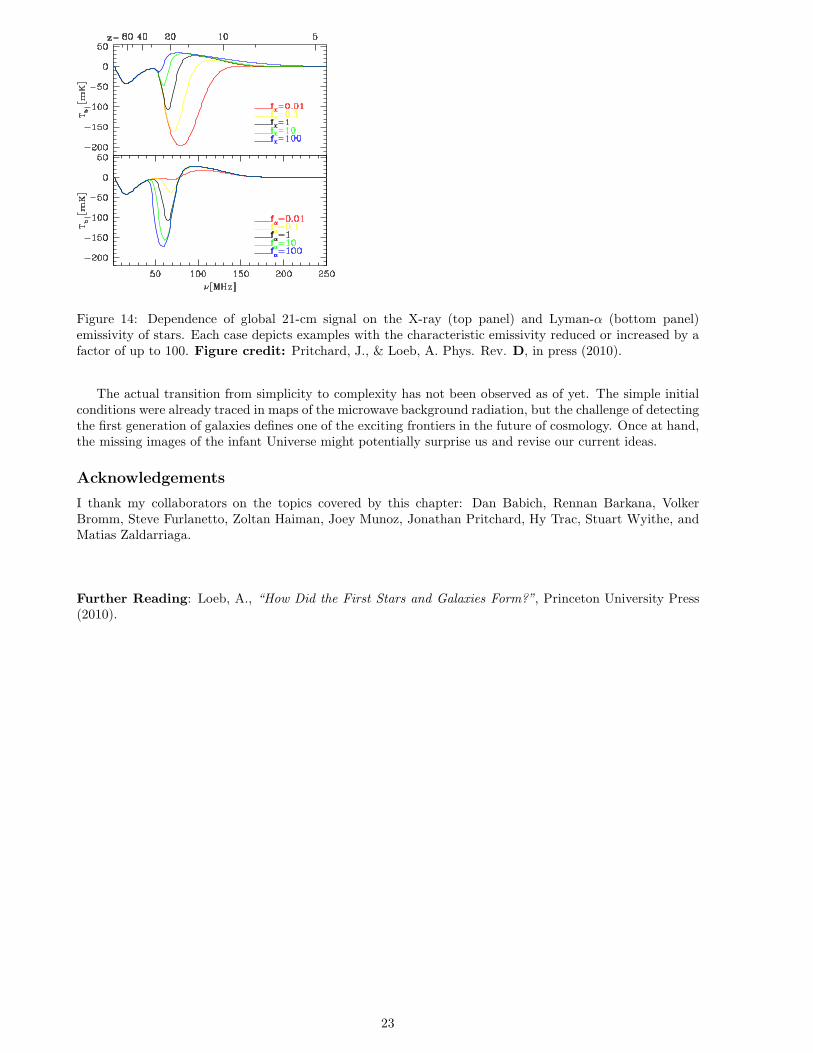
Figure 14: Dependence of global 21-cm signal on the X-ray (top panel) and Lyman-α (bottom panel)emissivity of stars. Each case depicts examples with the characteristic emissivity reduced or increased by afactor of up to 100. Figure credit: Pritchard, J., & Loeb, A. Phys. Rev. D, in press (2010).

The actual transition from simplicity to complexity has not been observed as of yet. The simple initialconditions were already traced in maps of the microwave background radiation, but the challenge of detectingthe first generation of galaxies defines one of the exciting frontiers in the future of cosmology. Once at hand,the missing images of the infant Universe might potentially surprise us and revise our current ideas.

Acknowledgements

I thank my collaborators on the topics covered by this chapter: Dan Babich, Rennan Barkana, VolkerBromm, Steve Furlanetto, Zoltan Haiman, Joey Munoz, Jonathan Pritchard, Hy Trac, Stuart Wyithe, andMatias Zaldarriaga.

Further Reading: Loeb, A., “How Did the First Stars and Galaxies Form?”, Princeton University Press(2010).

23