Embed Size (px)
Citation preview
The Relational Database Model
2
Objectives
• How relational database model takes a logical view of data
• Understand how the relational model’s basic components are relations implemented through tables in a relational DBMS
• How relations are organized in tables composed of rows (tuples) and columns (attributes)
• Use relational database operators, the data dictionary, and the system catalog
• How data redundancy is handled in the relational database model
• Why indexing is important
3
A Logical View of Data• Relational model
– Enables programmer to view data logically rather than physically
• Table – Has advantages of structural and data
independence– Resembles a file from conceptual point of view– Easier to understand than its hierarchical and
network database predecessors
4
Tables and Their Characteristics
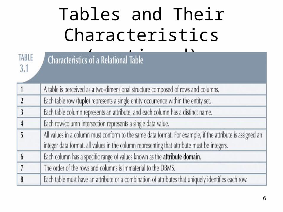
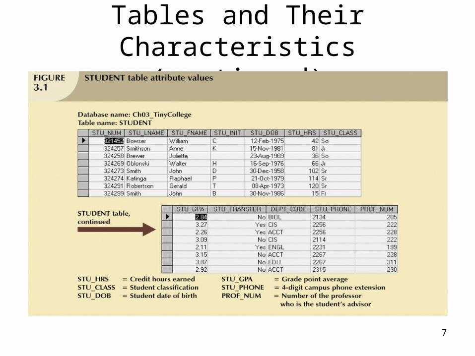
• Table: two-dimensional structure composed of rows and columns
• Contains group of related entities = an entity set– Terms entity set and table are often used
interchangeably
5
Tables and Their Characteristics (continued)
• Table also called a relation because the relational model’s creator, Codd, used the term relation as a synonym for table
• Think of a table as a persistent relation:– A relation whose contents can be permanently
saved for future use
6
Tables and Their Characteristics (continued)
7
Tables and Their Characteristics (continued)
8
Keys
• Consists of one or more attributes that determine other attributes
• Primary key (PK) is an attribute (or a combination of attributes) that uniquely identifies any given entity (row)
• Key’s role is based on determination– If you know the value of attribute A, you can
look up (determine) the value of attribute B
9
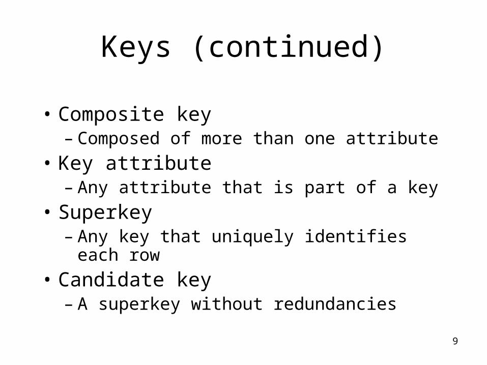
Keys (continued)
• Composite key– Composed of more than one attribute
• Key attribute– Any attribute that is part of a key
• Superkey– Any key that uniquely identifies each row
• Candidate key – A superkey without redundancies
10
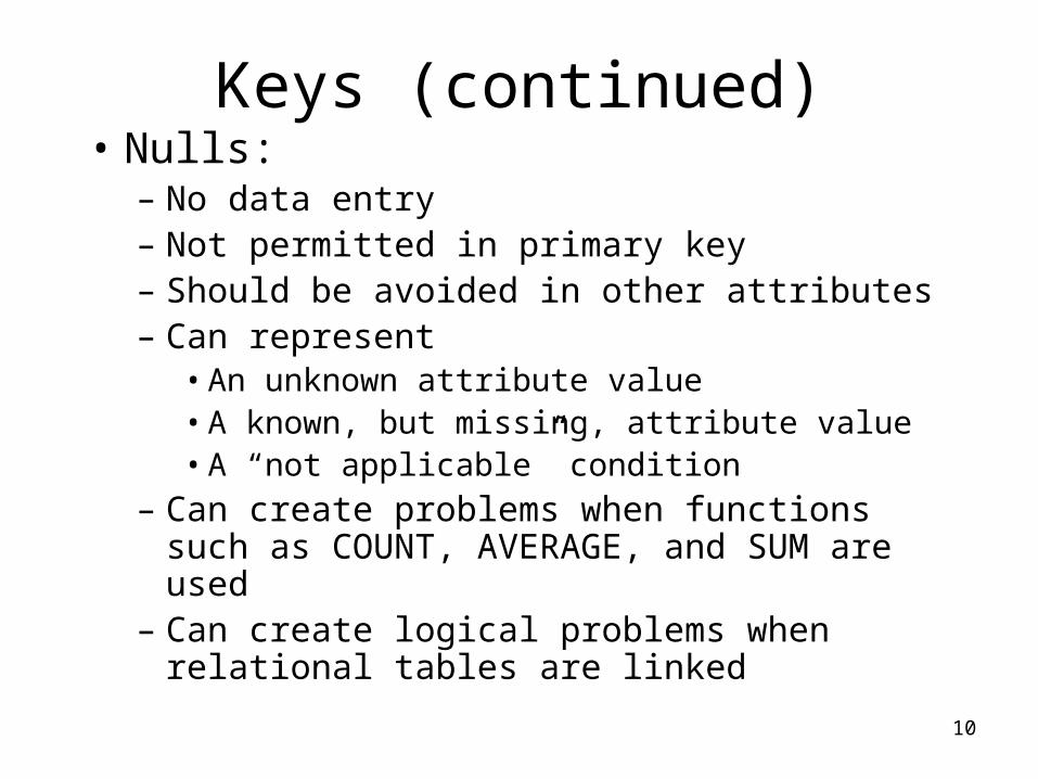
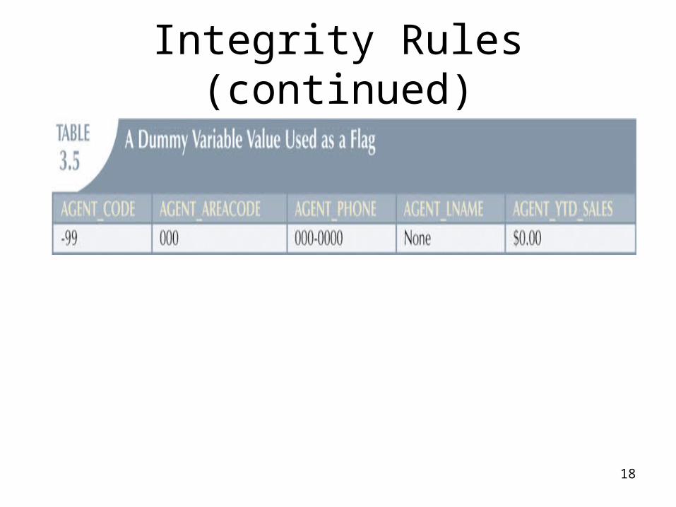
Keys (continued)• Nulls:
– No data entry– Not permitted in primary key– Should be avoided in other attributes– Can represent
• An unknown attribute value• A known, but missing, attribute value• A “not applicable” condition
– Can create problems when functions such as COUNT, AVERAGE, and SUM are used
– Can create logical problems when relational tables are linked
11
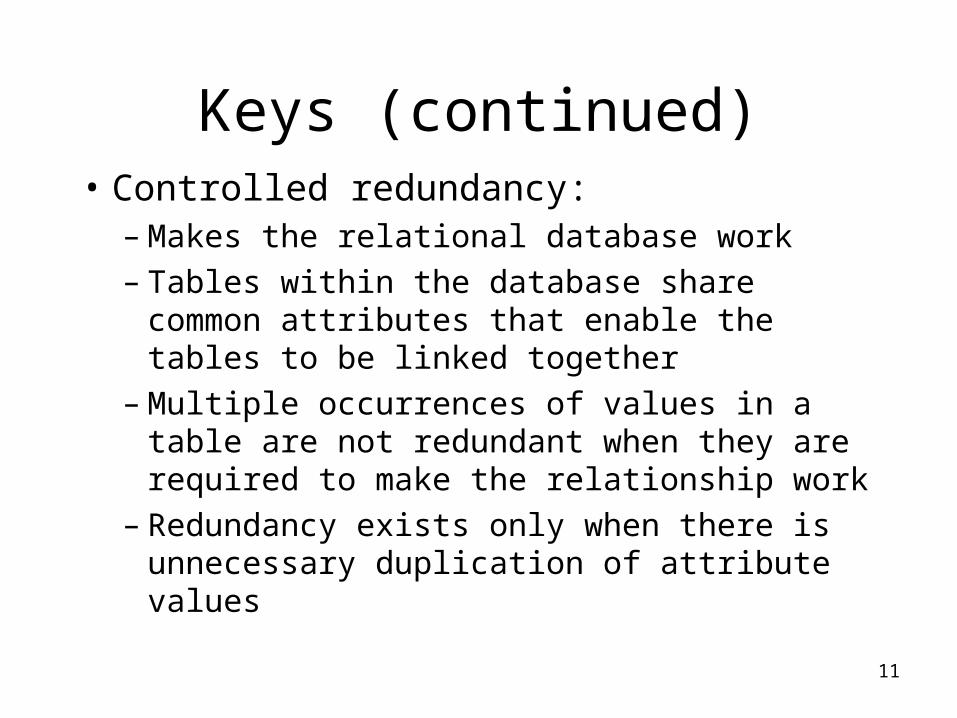
Keys (continued)• Controlled redundancy:
– Makes the relational database work– Tables within the database share common
attributes that enable the tables to be linked together
– Multiple occurrences of values in a table are not redundant when they are required to make the relationship work
– Redundancy exists only when there is unnecessary duplication of attribute values
12
Keys (continued)
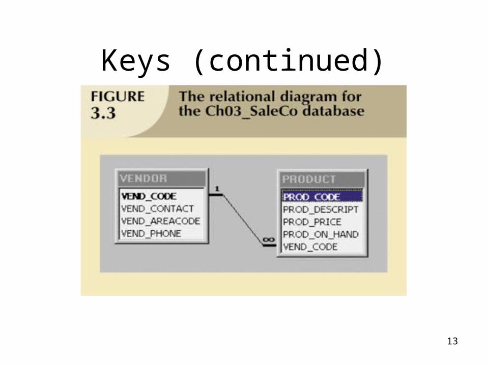
13
Keys (continued)
14
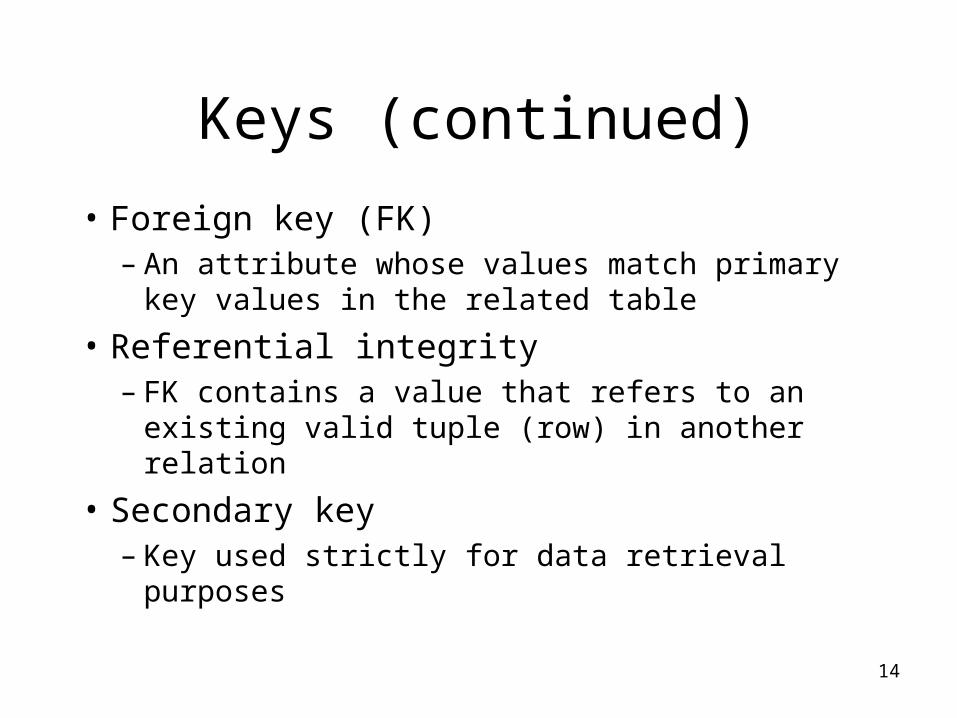
Keys (continued)
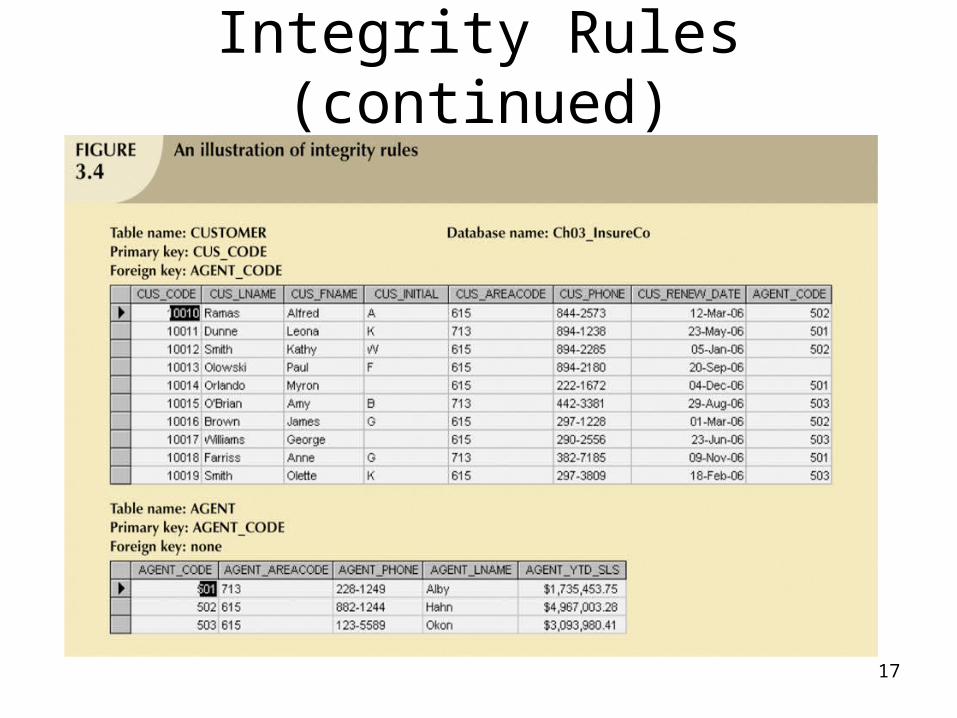
• Foreign key (FK) – An attribute whose values match primary
key values in the related table
• Referential integrity – FK contains a value that refers to an
existing valid tuple (row) in another relation
• Secondary key – Key used strictly for data retrieval purposes
15
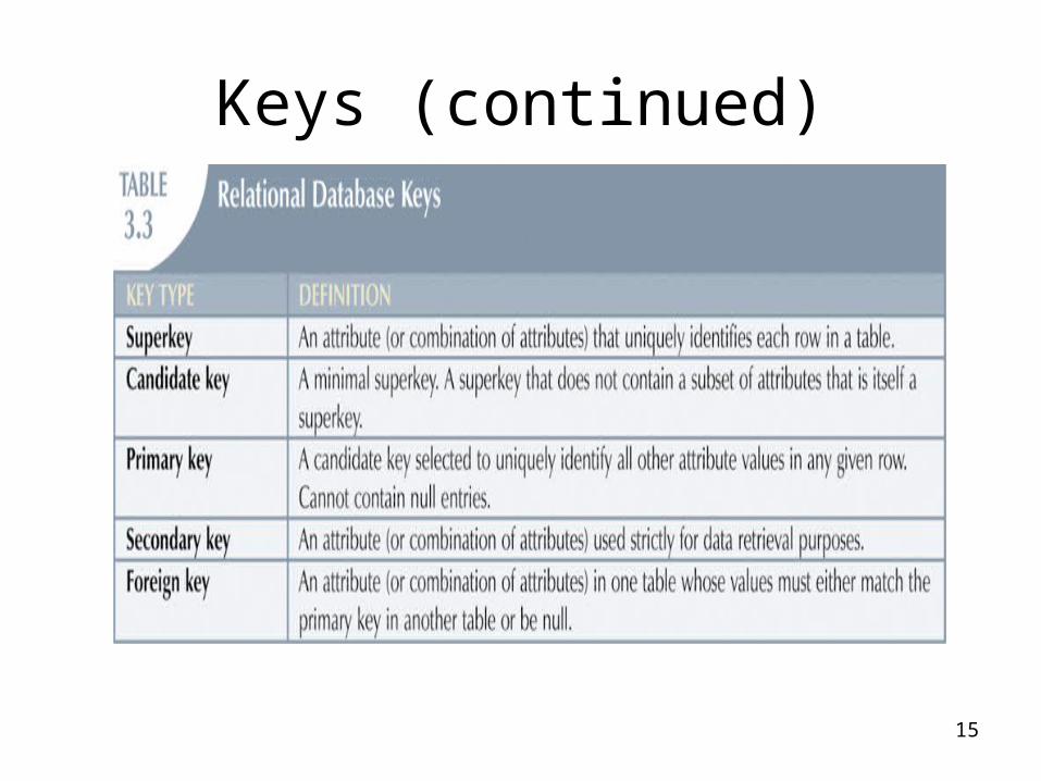
Keys (continued)
16
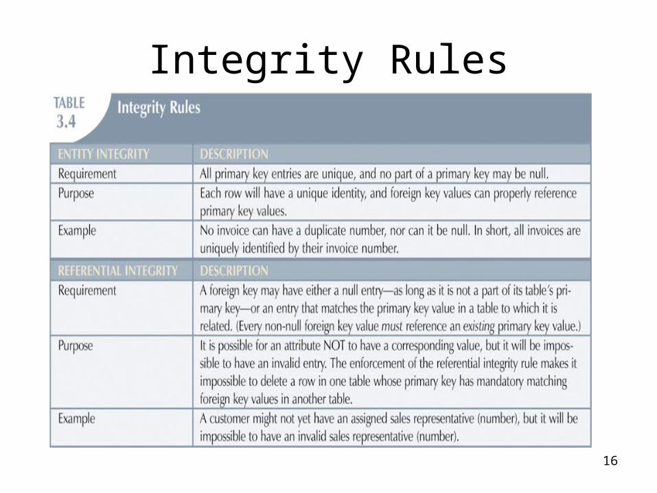
Integrity Rules
17
Integrity Rules (continued)
18
Integrity Rules (continued)
19
Relational Database Operators
• Relational algebra
– Defines theoretical way of manipulating table contents using relational operators
– Use of relational algebra operators on existing tables (relations) produces new relations
20
Relational Algebra Operators (continued)
• UNION
• INTERSECT
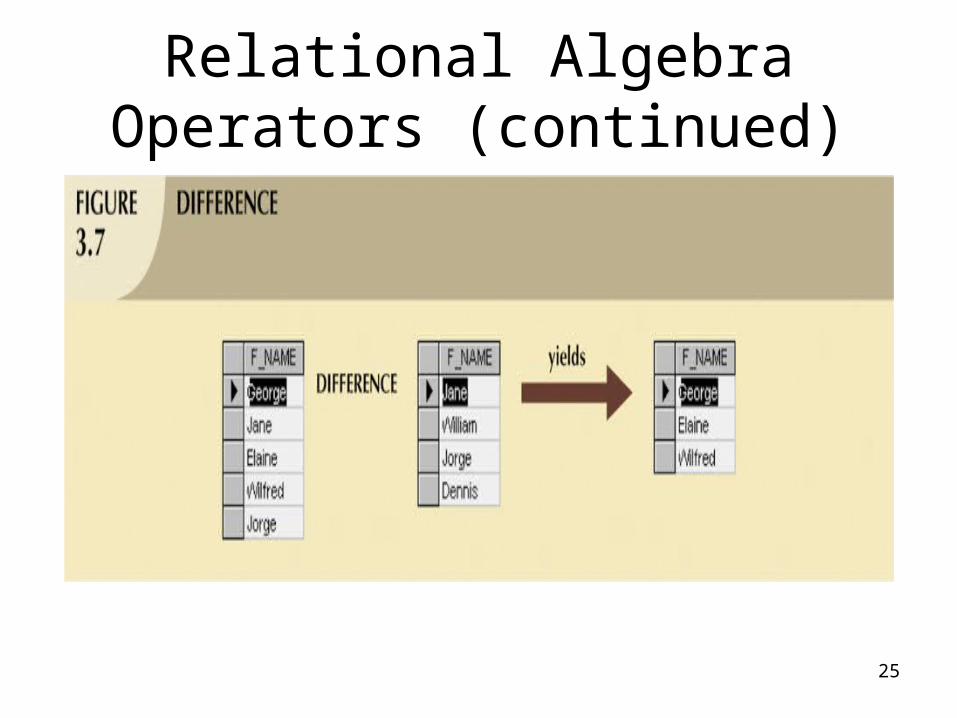
• DIFFERENCE
• PRODUCT
• SELECT
• PROJECT
• JOIN
• DIVIDE
21
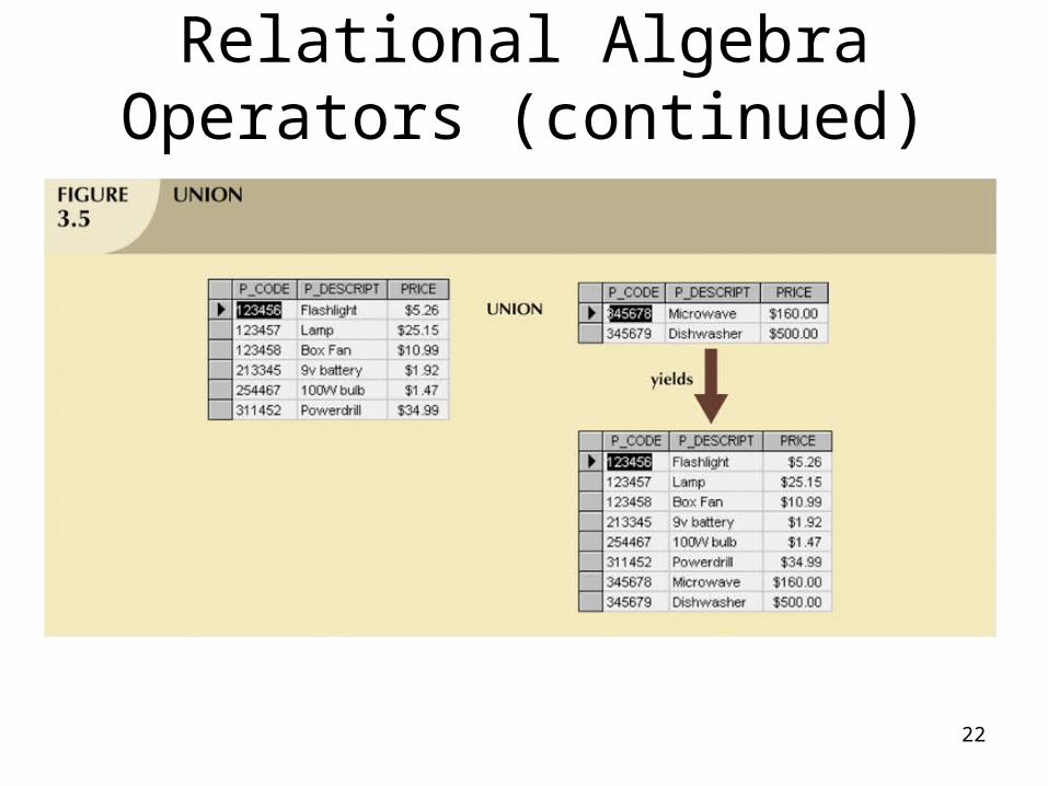
Relational Algebra Operators (continued)
• Union:– Combines all rows from two tables, excluding
duplicate rows
– Tables must have the same attribute characteristics
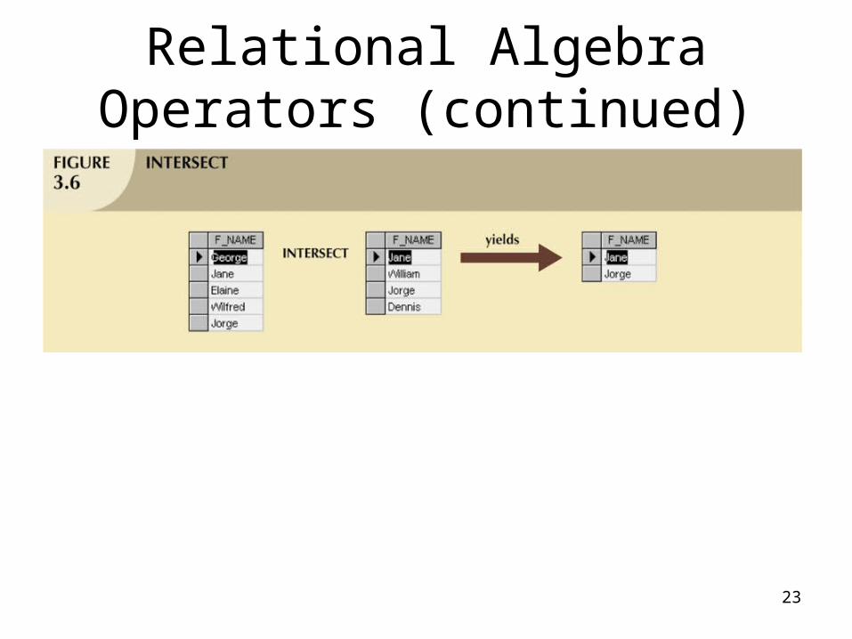
• Intersect:– Yields only the rows that appear in both tables
22
Relational Algebra Operators (continued)
23
Relational Algebra Operators (continued)
24
Relational Algebra Operators (continued)
• Difference– Yields all rows in one table not found in the
other table — that is, it subtracts one table from the other
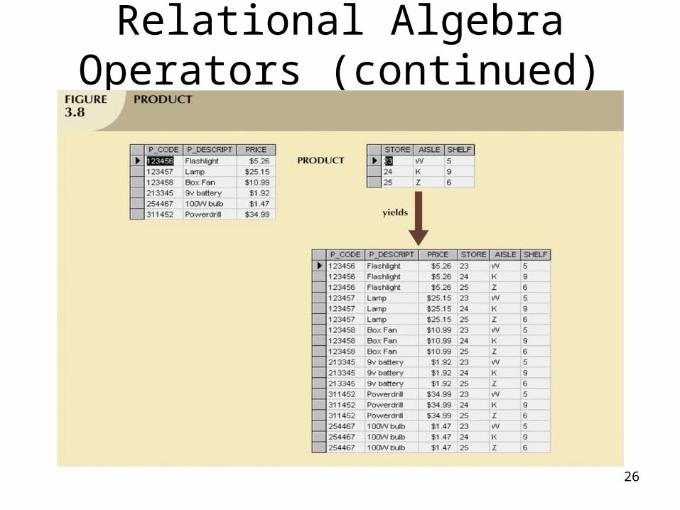
• Product– Yields all possible pairs of rows from two
tables• Also known as the Cartesian product
25
Relational Algebra Operators (continued)
26
Relational Algebra Operators (continued)
27
Relational Algebra Operators (continued)
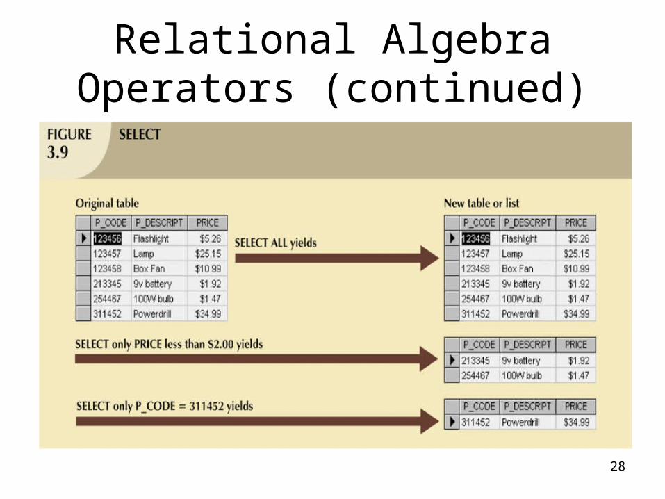
• Select– Yields values for all rows found in a table– Can be used to list either all row values or it
can yield only those row values that match a specified criterion
– Yields a horizontal subset of a table
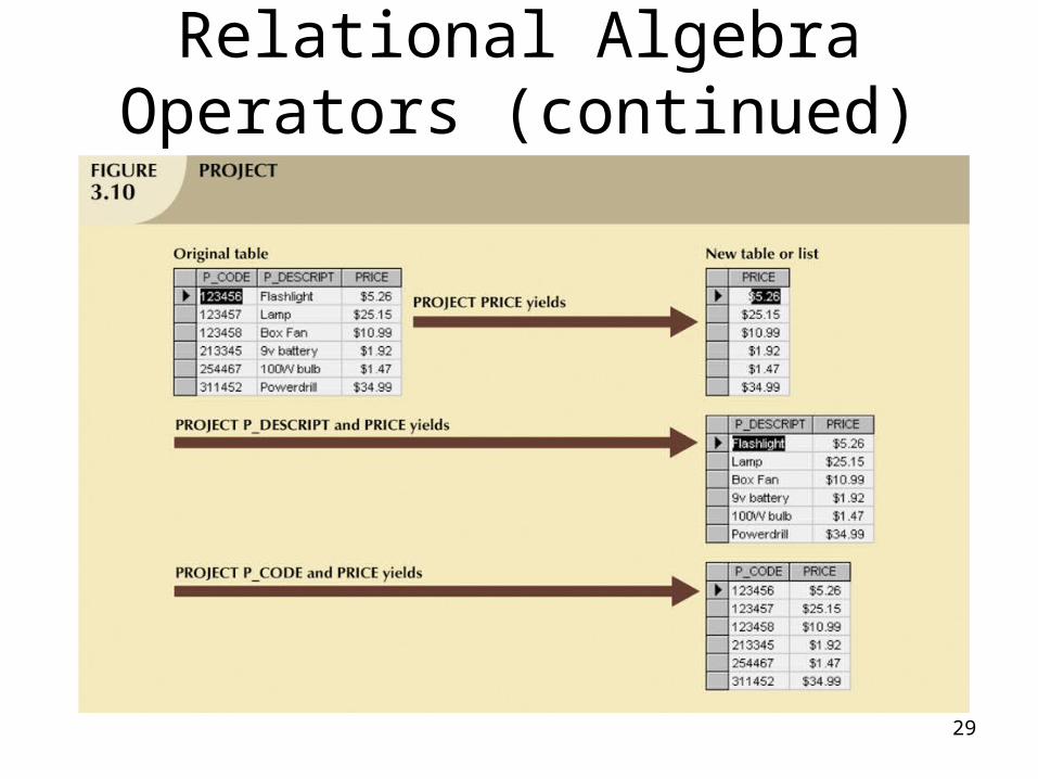
• Project– Yields all values for selected attributes– Yields a vertical subset of a table
28
Relational Algebra Operators (continued)
29
Relational Algebra Operators (continued)
30
Relational Algebra Operators (continued)
• Join– Allows information to be combined from two or
more tables– Real power behind the relational database,
allowing the use of independent tables linked by common attributes
31
Relational Algebra Operators (continued)
32
Relational Algebra Operators (continued)
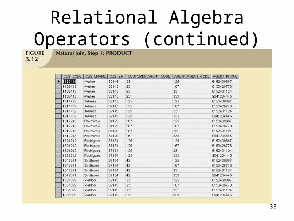
• Natural Join– Links tables by selecting only rows with
common values in their common attribute(s)
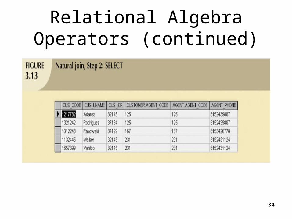
– Result of a three-stage process:• PRODUCT of the tables is created• SELECT is performed on Step 1 output to yield only the
rows for which the AGENT_CODE values are equal– Common column(s) are called join column(s)
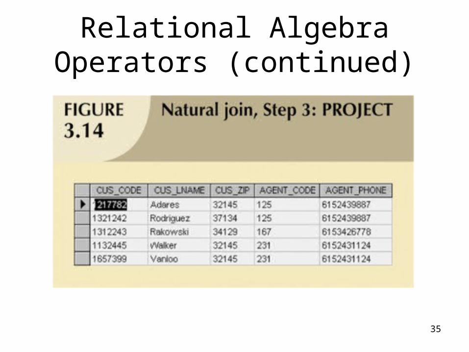
• PROJECT is performed on Step 2 results to yield a single copy of each attribute, thereby eliminating duplicate columns
33
Relational Algebra Operators (continued)
34
Relational Algebra Operators (continued)
35
Relational Algebra Operators (continued)
36
Relational Algebra Operators (continued)
• Natural Join:– Final outcome yields table that
• Does not include unmatched pairs
• Provides only copies of matches
– If no match is made between the table rows• the new table does not include the
unmatched row
37
Relational Algebra Operators (continued)
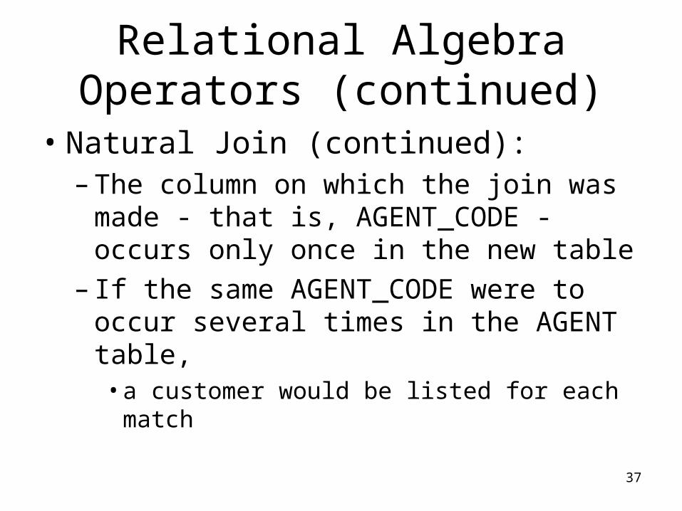
• Natural Join (continued):– The column on which the join was made -
that is, AGENT_CODE - occurs only once in the new table
– If the same AGENT_CODE were to occur several times in the AGENT table, • a customer would be listed for each match
38
Relational Algebra Operators (continued)
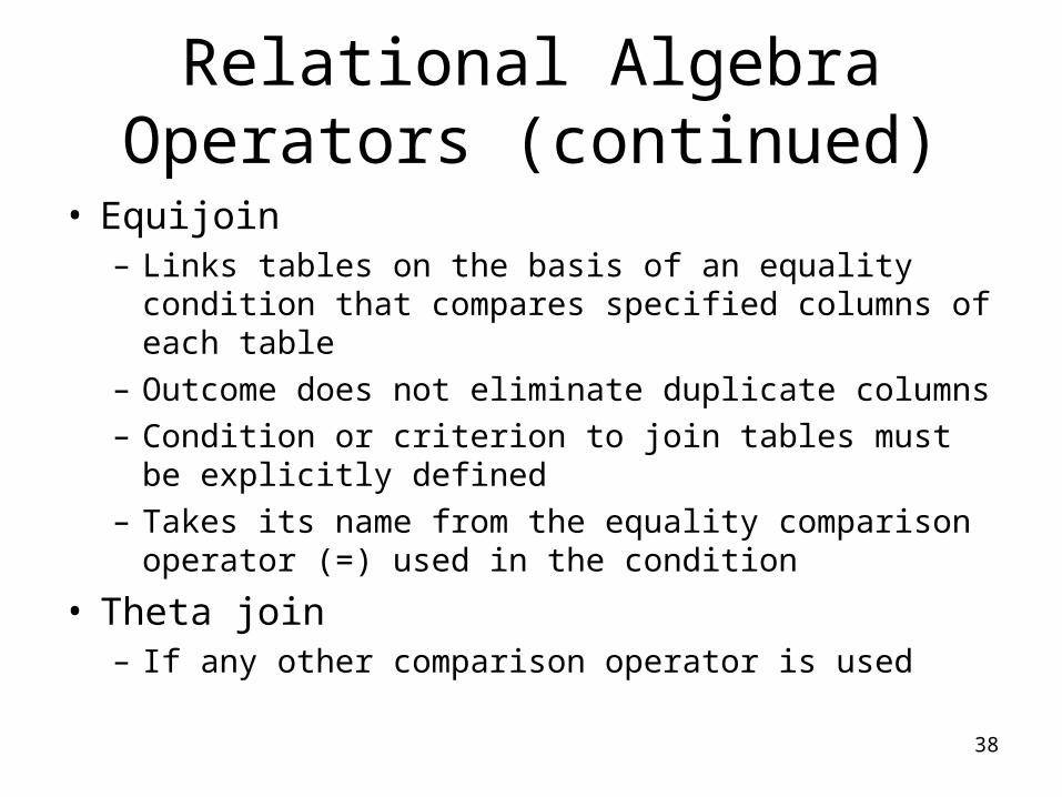
• Equijoin– Links tables on the basis of an equality condition that
compares specified columns of each table– Outcome does not eliminate duplicate columns– Condition or criterion to join tables must be explicitly
defined– Takes its name from the equality comparison operator
(=) used in the condition
• Theta join– If any other comparison operator is used
39
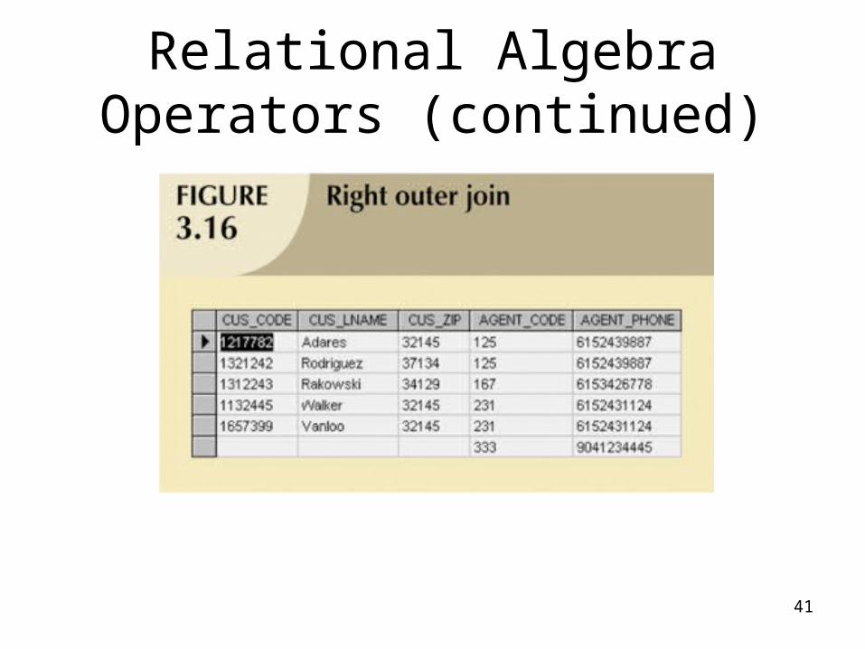
Relational Algebra Operators (continued)
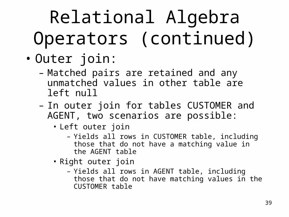
• Outer join:– Matched pairs are retained and any unmatched
values in other table are left null– In outer join for tables CUSTOMER and AGENT,
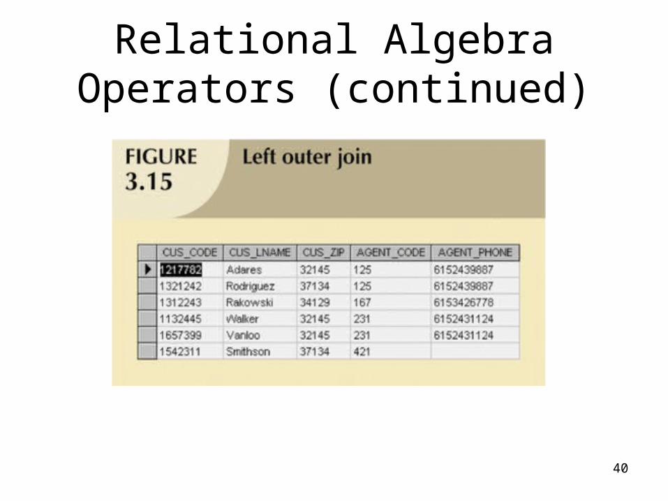
two scenarios are possible:• Left outer join
– Yields all rows in CUSTOMER table, including those that do not have a matching value in the AGENT table
• Right outer join – Yields all rows in AGENT table, including those that do not
have matching values in the CUSTOMER table
40
Relational Algebra Operators (continued)
41
Relational Algebra Operators (continued)
42
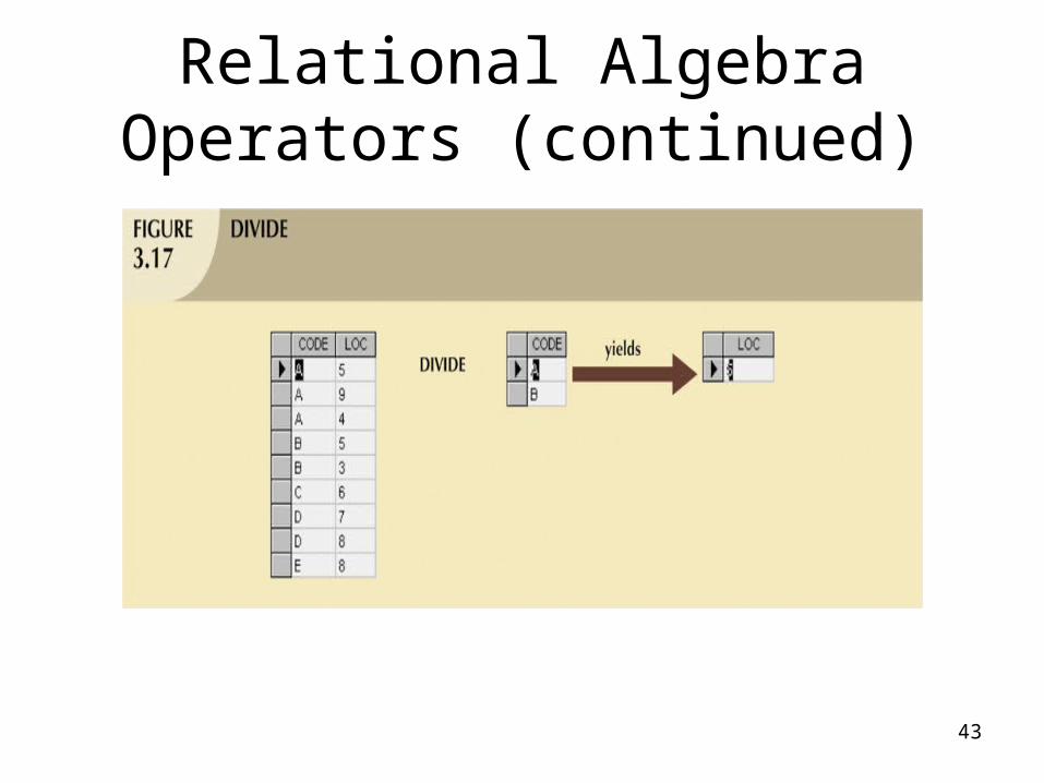
Relational Algebra Operators (continued)
• DIVIDE requires the use of one single-column table and one two-column table
43
Relational Algebra Operators (continued)
44
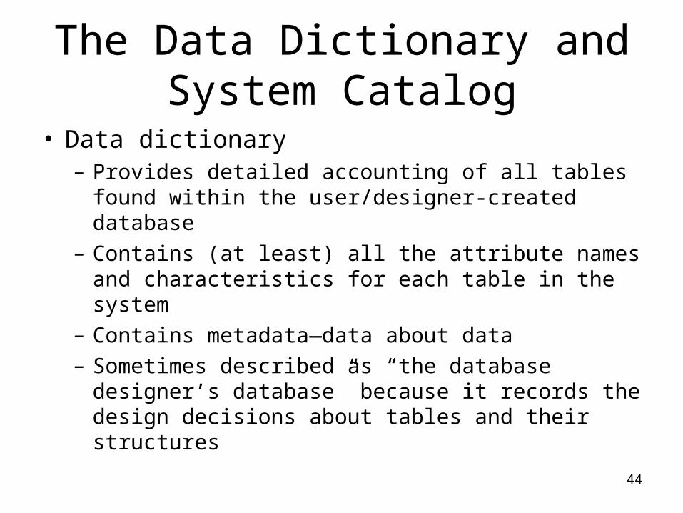
The Data Dictionary and System Catalog
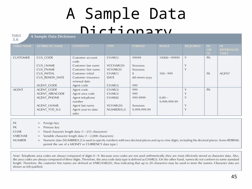
• Data dictionary – Provides detailed accounting of all tables found within
the user/designer-created database– Contains (at least) all the attribute names and
characteristics for each table in the system– Contains metadata—data about data– Sometimes described as “the database designer’s
database” because it records the design decisions about tables and their structures
45
A Sample Data Dictionary
46
The Data Dictionary and System Catalog (continued)
• System catalog – Contains metadata– Detailed system data dictionary that describes
all objects within the database– Terms “system catalog” and “data dictionary”
are often used interchangeably– Can be queried just like any user/designer-
created table
47
Relationships within the Relational Database
• 1:M relationship – Relational modeling ideal– Should be the norm in any relational database design
• 1:1 relationship– Should be rare in any relational database design
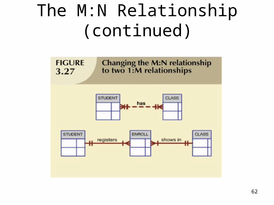
• M:N relationships – Cannot be implemented as such in the relational
model– M:N relationships can be changed into two 1:M
relationships
48
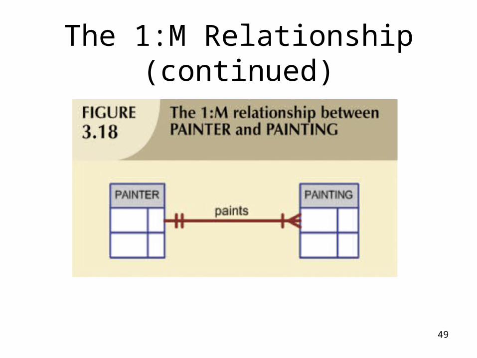
The 1:M Relationship
• Relational database norm
• Found in any database environment
49
The 1:M Relationship (continued)
50
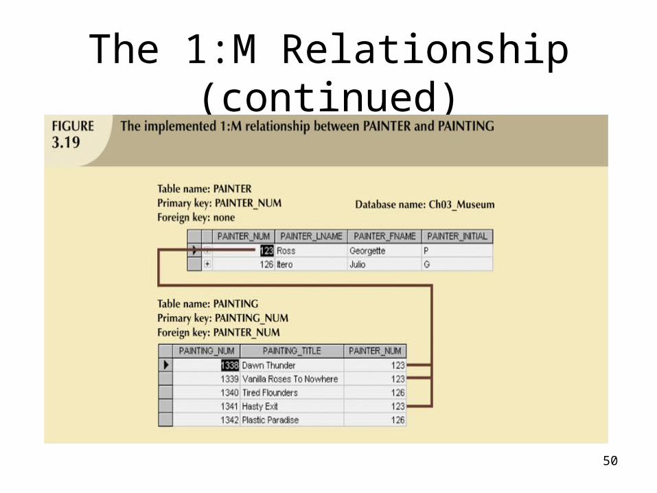
The 1:M Relationship (continued)
51
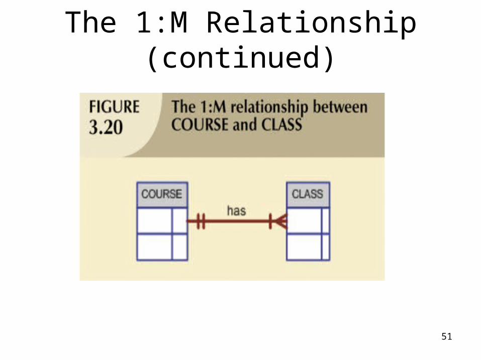
The 1:M Relationship (continued)
52
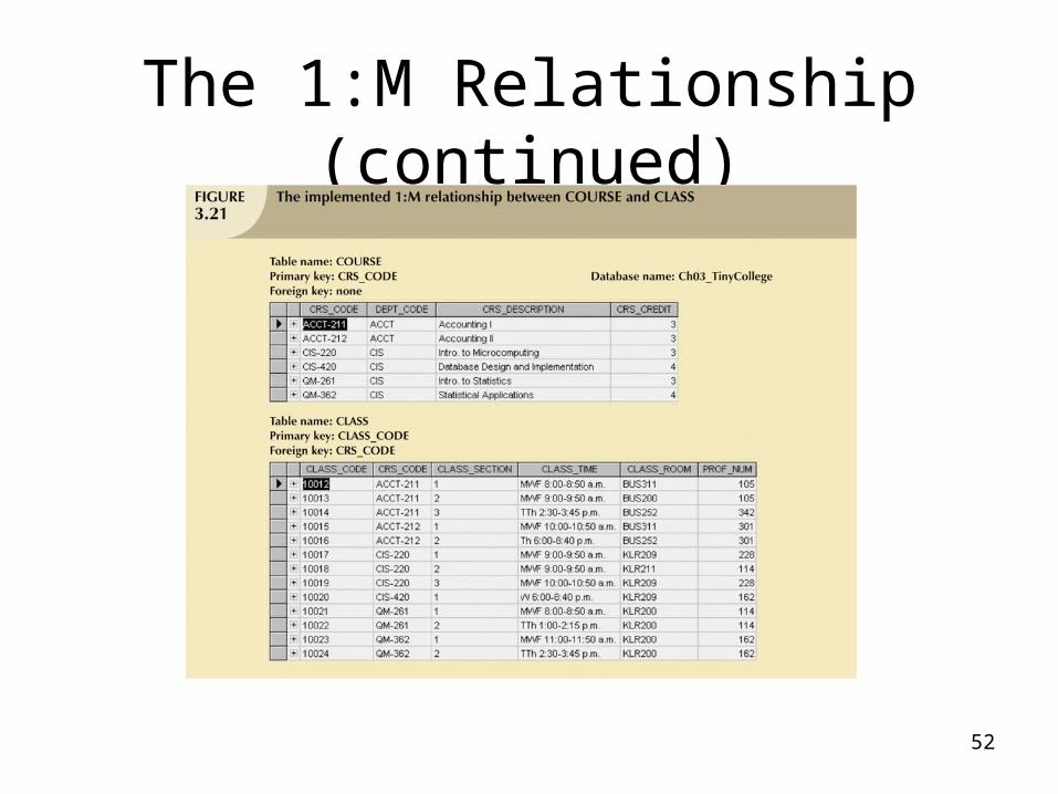
The 1:M Relationship (continued)
53
The 1:1 Relationship
• One entity can be related to only one other entity, and vice versa
• Sometimes means that entity components were not defined properly
• Could indicate that two entities actually belong in the same table
• As rare as 1:1 relationships should be, certain conditions absolutely require their use
54
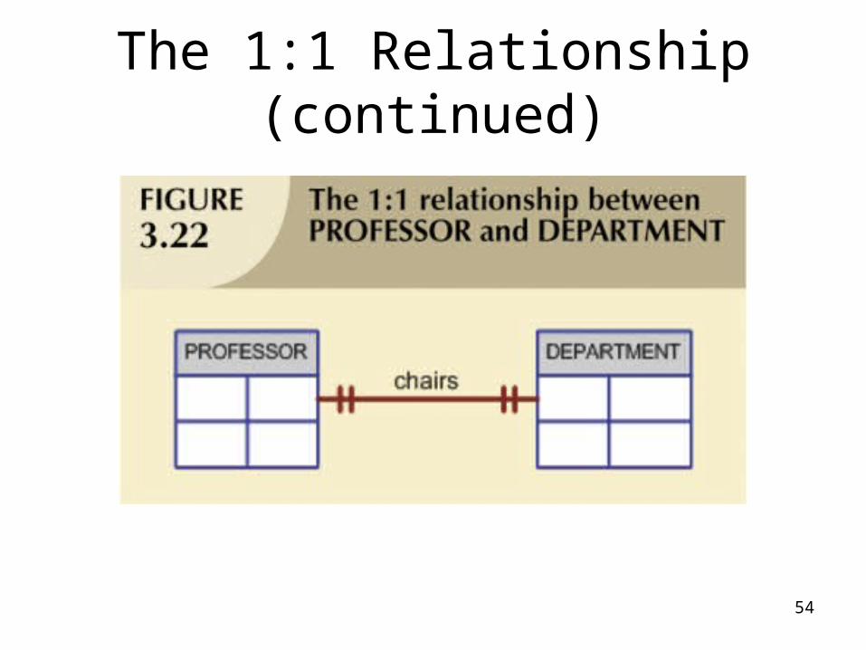
The 1:1 Relationship (continued)
55
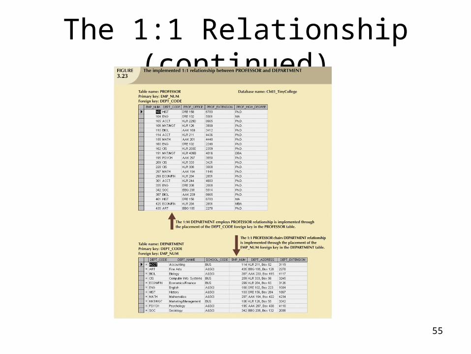
The 1:1 Relationship (continued)
56
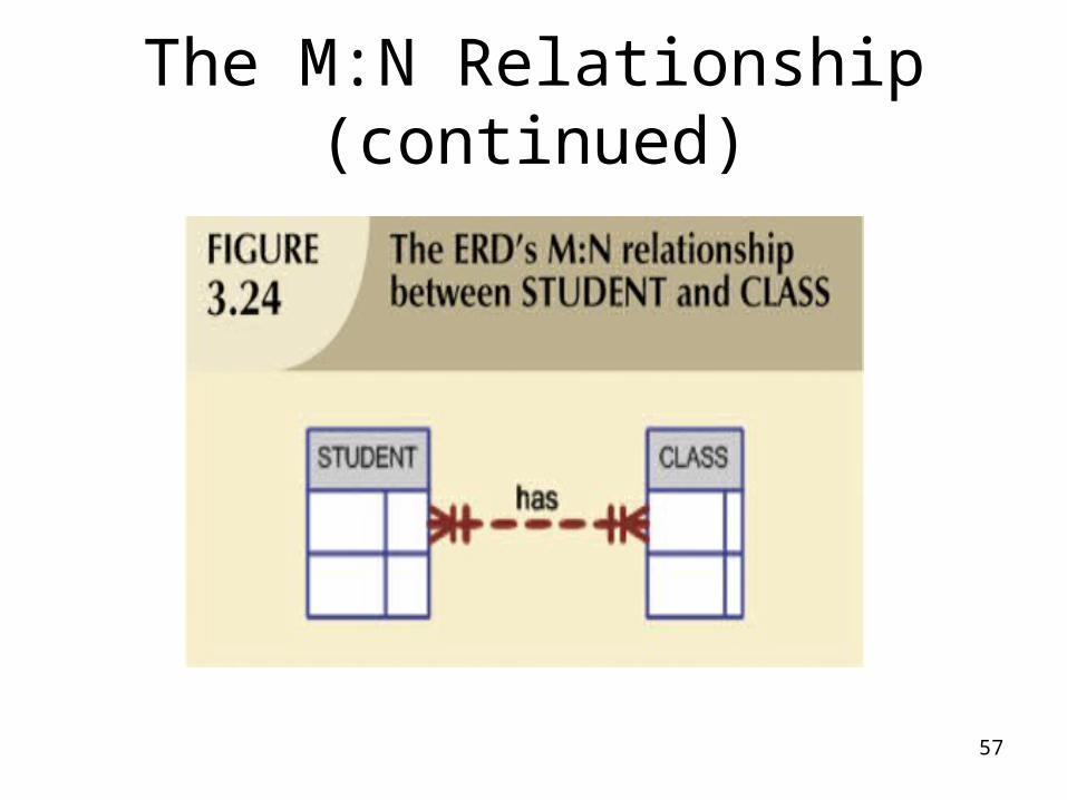
The M:N Relationship
• Can be implemented by breaking it up to produce a set of 1:M relationships
• Can avoid problems inherent to M:N relationship by creating a composite entity or bridge entity
57
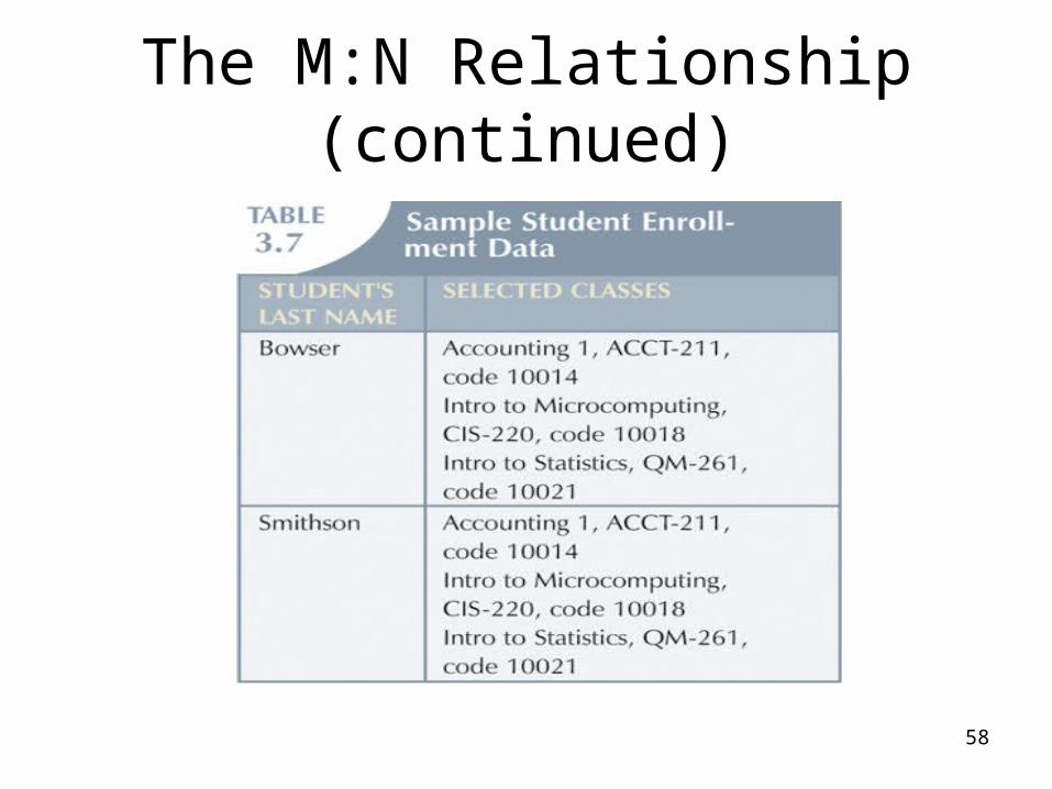
The M:N Relationship (continued)
58
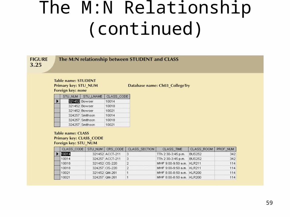
The M:N Relationship (continued)
59
The M:N Relationship (continued)
60
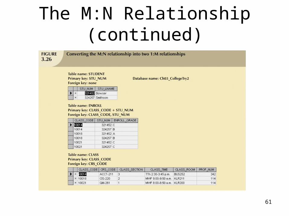
The M:N Relationship (continued)
• Implementation of a composite entity• Yields required M:N to 1:M conversion• Composite entity table must contain at
least the primary keys of original tables• Linking table contains multiple
occurrences of the foreign key values• Additional attributes may be assigned
as needed
61
The M:N Relationship (continued)
62
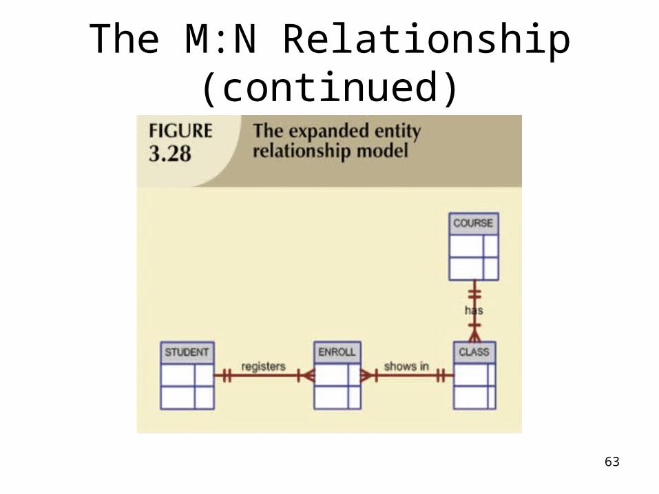
The M:N Relationship (continued)
63
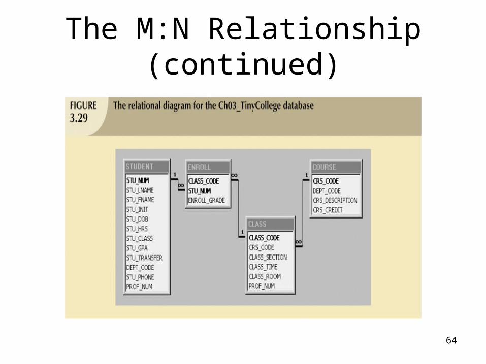
The M:N Relationship (continued)
64
The M:N Relationship (continued)
65
Data Redundancy Revisited
• Data redundancy leads to data anomalies– Such anomalies can destroy the effectiveness
of the database
• Foreign keys– Control data redundancies by using common
attributes shared by tables– Crucial to exercising data redundancy control
• Sometimes, data redundancy is necessary
66
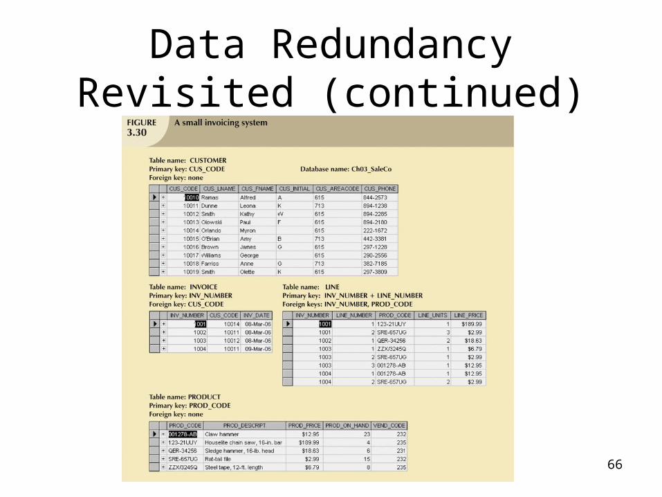
Data Redundancy Revisited (continued)
67
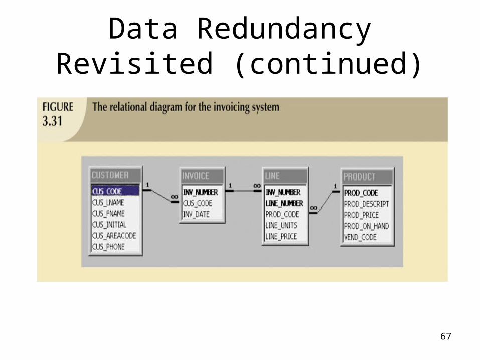
Data Redundancy Revisited (continued)
68
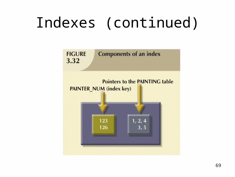
Indexes• Arrangement used to logically access rows
in a table• Index key
– Index’s reference point
– Points to data location identified by the key
• Unique index– Index in which the index key can have only one
pointer value (row) associated with it
• Each index is associated with only one table
69
Indexes (continued)
70
Codd’s Relational Database Rules
• In 1985, Codd published a list of 12 rules to define a relational database system
• The reason was the concern that many vendors were marketing products as “relational” even though those products did not meet minimum relational standards

71
Codd’s Relational Database Rules (Continued)
72
Summary
• Tables are basic building blocks of a relational database
• Keys are central to the use of relational tables• Keys define functional dependencies
– Superkey– Candidate key– Primary key– Secondary key– Foreign key
73
Summary (continued)
• Each table row must have a primary key which uniquely identifies all attributes
• Tables can be linked by common attributes. Thus, the primary key of one table can appear as the foreign key in another table to which it is linked
• The relational model supports relational algebra functions: SELECT, PROJECT, JOIN, INTERSECT, UNION, DIFFERENCE, PRODUCT, and DIVIDE.
• Good design begins by identifying appropriate entities and attributes and the relationships among the entities. Those relationships (1:1, 1:M, and M:N) can be represented using ERDs.