The Relationship between Vehicle Yaw Acceleration Response andSteering Velocity for Steering Control

M.J. Thoresson; T.R. Botha; P.S. Els

Department of Mechanical and Aeronautical Engineering, University of Pretoria, Pretoria 0002, SouthAfrica

Abstract

This paper proposes a novel concept for the modelling of a vehicle steering driver model for pathfollowing. The proposed steering driver reformulates and applies the Magic Formula, used for tyremodelling, to the vehicle's yaw acceleration vs. steering velocity response as a function of vehicle speed.

The path-following driver model was developed for use in gradient-based mathematical optimisation ofvehicle suspension characteristics for handling. Successful application of gradient-based optimisationdepends on the availability of good gradient information. This requires a robust driver model that canensure completion of the required handling manoeuvre, even when the vehicle handling is poor.

The steering driver is applied to a non-linear full vehicle model of a Sports Utility Vehicle, performing asevere double lane change manoeuvre. Simulation results show excellent correlation with test results. Theproposed driver model is robust and well suited to gradient-based optimisation of vehicle handling.

Keywords: driver model, Magic Formula, steering response, tyre characteristics, handling, mathematicaloptimisation.

1. Introduction

The use of lateral path following driver models for the simulation of closed loop vehiclehandling manoeuvres is vital. However, great difficulty is often experienced indetermining the gain parameters for a stable driver at all realistic vehicle speeds, andvehicle parameters.

The primary reason for requiring a driver model in the present study is for theoptimisation of an off-road vehicle's suspension system. The suspension characteristicsare to be optimised for handling, while performing the closed loop ISO 3888-1(International Organisation for Standardisation, 2004) severe double lane changemanoeuvre. The driver model thus has to be robust for various suspension setups, andperform only one simulation to return the objective function value. Therefore steeringcontrollers with learning capability will not be considered, as the suspension could bevastly different from one simulation to the next. Only lateral path following is consideredin this preliminary research, as the double lane change manoeuvre is normally performedat a constant vehicle speed. Furthermore the main purpose of the driver model is toenable successful completion of the handling manoeuvre, so that good gradient

information can be determined, especially when the suspension settings are far from theoptimum settings for handling. Accurate representations of real human driver behaviourunder these conditions are less important than the successful completion of themanoeuvre.

The current research is concerned with the development of a controllable suspensionsystem for Sports Utility Vehicles (SUV's). The suspension system has to be modelled,and the handling dynamics simulated, for widely varying suspension settings. The vehiclein question has a comparatively soft suspension, coupled to a high centre of gravity,resulting in large suspension deflections when performing the double lane changemanoeuvre. This large suspension deflection results in highly unstable vehicle behaviour,eliminating the use of driver models suited to vehicles with minimal suspensiondeflection. Steady state rollover calculations also show that the vehicle will roll overbefore it will slide.

A robust driver model is difficult to achieve, especially when suspension spring anddamper characteristics are allowed to vary over a wide range. The determination of drivermodel parameters become especially complex when accurate, non-linear full vehiclemodels, with large suspension travel, are to be controlled in proximity to the handlinglimits of the vehicle.

This research proposes a novel lateral path-following driver model based on therelationship between vehicle yaw response and non-linear tyre characteristics. The non-linearity of the tyre characteristics is replicated for the steering model’s parameters. Thenon-linear response of the vehicle is captured by fitting the Magic Formula (frequentlyused for tyre lateral force vs. slip angle modelling) to the vehicle’s yaw acceleration vs.steering velocity for different vehicle speeds.

Previous research into lateral vehicle model drivers is now discussed, followed by themathematical vehicle model. The characterization of the vehicle's dynamics, with theMagic Formula driver model, and the implementation thereof completes the paper.

An extensive overview of driver models for vehicle dynamics applications is given byPlöchl and Edelmann (2007). Many different driver models have been proposed, most ofwhich have specific applications and are difficult to generalise for all requirements.

Snider (2009) evaluated various driver models in CarSim (2011). The driver modelsranged from simple kinematic and geometric models, used by various autonomousvehicles (Thrun et al., 2006 and Urmson et al., 2008), to more complex dynamic modelsbased on optimal control theory (Tewari, 2002). Snider (2009) concluded that the drivermodels can be tuned to suit a specific range of conditions. With most exhibiting acompromise between low speed performance and high speed stability.

Sharp, Casanova and Symonds (2000) implement a linear, multiple preview pointcontroller, with steering saturation limits mimicking tyre saturation, for vehicle tracking.The vehicle model used is a 5-degree-of-freedom (dof) model, with non-linear MagicFormula tyre characteristics, but no suspension deflection. This model is successfully

applied to a Formula One vehicle performing a lane change manoeuvre. Gordon, Bestand Dixon (2002) make use of a novel method, based on convergent vector fields, tocontrol the vehicle along desired routes. The vehicle model is a 3-dof vehicle, with non-linear Magic Formula tyre characteristics, but with no suspension deflection included.The driver model is successfully applied to lane change manoeuvres. The primarysimilarity between these methods is that vehicle models with no suspension deflectionwere used.

Prokop (2001) implements a PID (Proportional Integral Derivative) prediction model fortracking control of a bicycle model vehicle. The driver model makes use of a driver plantmodel that is representative of the actual vehicle. The driver plant increases withcomplexity to perform the required dynamic manoeuvre, from a point mass to a two trackmodel with elastokinematic suspension. This model is then optimised with the SQP(Sequential Quadratic Programming) optimisation algorithm for each time step. Thisapproach, however, becomes computationally expensive, when optimisation of thevehicle's handling is to be considered.

A typical simple linearised single point path following driver model is discussed byGenta (1997). This type of driver model is frequently used in the simulation of vehiclehandling.

For the current research several driver model approaches were implemented, but withlimited success. Due to the unsuccessful implementation of these driver models forsteering control, it was decided to characterize the whole vehicle system, using step steer,and ramp steer inputs, and observe various vehicle parameters. This lead to the discoverythat the relationship between vehicle yaw acceleration vs. steering rate for various vehiclespeeds appeared very similar to the side force vs. slip angle characteristics of the tyres.With this discovery it was decided to implement the proposed novel driver model, withthe gain factor modelled with the Pacejka Magic Formula, normally used for tyre data.

2. Mathematical Vehicle Model

For the simulation performed in this study, a Land Rover Defender 110 is modelled inMSC.ADAMS View with standard suspension settings, as a baseline. The non-linearMSC.ADAMS Pacejka 89 tyre model (Bakker, Pacejka and Linder, 1989) is fitted tomeasured tyre data, and used within the model. The tyre's vertical dynamics and loaddependent lateral dynamics are considered in this model. The longitudinal dynamicbehaviour of the tyres and vehicle is not considered because the vehicle is driven atconstant speed. The vehicle body is modelled as two rigid bodies connected along the rollaxis at the chassis height, by a revolute joint and a torsional spring, in order to bettercapture the vehicle dynamics due to body torsion in roll. The anti-roll bar is modelled asa torsional spring between the two rear trailing arms to be representative of the actualanti-roll bar's effect. The bump and rebound stops are modelled with non-linear splines,as force elements between the axles and vehicle body. The suspension bushings aremodelled as kinematic joints with torsional spring characteristics that are representativeof the actual vehicle's suspension joint characteristics, in an effort to speed up the

solution time, and help decrease numerical noise. The baseline vehicle's springs anddampers are modelled with experimentally determined non-linear splines. The vehicle'scentre of gravity (cg) height and moments of inertia were also measured by Uys et al.(2005) and used within the model. Provision is made to vary the spring and dampercharacteristics over a wide range, for optimisation purposes. Figure 1 indicates thekinematic modelling of the rear and front suspensions. The complete model consists of 15unconstrained degrees of freedom, 16 moving parts, 6 spherical joints, 8 revolute joints, 7Hooke's joints, and one motion defined by the steering driver. The unconstrained degreesof freedom are indicated in table 1.

Table 1 - MSC.ADAMS vehicle model's unconstrained degrees of freedom

Body Degrees of Freedom Associated MotionsVehicle Body 7 body torsion

(2 rigid bodies) longitudinal, lateral, verticalroll, pitch, yaw

Front Axle 2 roll, verticalRear Axle 2 roll, vertical

Wheels 4 x 1 rotation

The speed control is modelled as a variable force attached to the body at wheel centreheight. The magnitude of this force depends on the difference between the instantaneousspeed and desired speed. Because the vehicle is four-wheel drive with open differentials,the vertical tyre force is measured at all tyres. If any tyre looses contact with the ground,the driving force to the vehicle is removed until all wheels are again in contact with theground. This MSC.ADAMS model is then linked to the Simulink based driver model thatreturns as outputs the desired vehicle speed and steering angle, calculated using thevehicle's dynamic response.

The vehicle model is validated against measured test data for the double lane changemanoeuvre at an entry speed of 65 km/h, where the steering input, as measured on thevehicle, is used to steer the simulation model. The results for the comparison between theMSC.ADAMS model and the measured results are presented in Figure 2, with excellentcorrelation achieved.

3. Driver Model Description

To investigate the relationship between vehicle response and steering inputs, simulationswere performed for various constant steering input rates, at various vehicle speeds withthe vehicle’s baseline suspension system. The results of some of these simulations aredisplayed in Figure 3. The plots indicate that the yaw acceleration attains a constant valuefor a significant part of the duration of the simulation, for each specific steer rate andvehicle speed, for almost all steer rates at low speeds and for low steer rates at highspeeds. It can also be noted that the response becomes larger as vehicle speed increasesfor the same steer rate. This increase in sensitivity is well known with modern vehiclesequipped with active steering systems which reduce the steer ratio to improve steeringstability at high vehicle speeds, such as BMW’s active steering system Qinchao et al(2011). As a result of the increase in sensitivity, lower steer rates are required at higher

speeds to generate the same yaw acceleration response. Thus, the use of lower steer ratesat higher speeds ensures that the yaw acceleration response still obtains a constant valuefor a significant part of the input duration. These constant values of the responsessuddenly reduce towards the end of the test. This sudden reduction is most likely due tothe tyre reaching its saturation level.

Since both the steer rate and vehicle speed would influence the time to reach tyresaturation, the yaw acceleration was therefore plotted against lateral acceleration ratherthan time. The lateral acceleration also gives a measure of the level of tyre saturation.Figure 4 shows the yaw acceleration vs. lateral acceleration as a function of steer rate fordifferent vehicle speeds. The figure better illustrates the near constant response obtainedby the yaw acceleration. The response stays fairly constant up to very high lateralaccelerations after which a sudden drop occurs (indicating that the tyre force issaturating).

Reymond et al. (2001), as well as Hugemann and Nickel (2002), showed that normaldrivers typically reached higher lateral accelerations as vehicle speeds increased. Thisincrease was however only up to a certain speed. After exceeding this speed they tendedto reach lower lateral accelerations with increasing speed to increase the safety marginavailable to them. In their tests conducted during normal driving the lateral accelerationseldomly exceeded 6 m/s2. Thus, the normal operating lateral accelerations of a vehiclecan be considered to be below 6 m/s2. If it is considered that the yaw accelerationresponse remains fairly constant below lateral acceleration of 6 m/s2, it can be said thatthe yaw acceleration obtains a steady state response during normal operating conditionsfor a specific vehicle speed and steer rate.

It is thus possible to obtain the steady state yaw acceleration response as a function ofsteer rate and vehicle speed. The steady state yaw acceleration vs. steer rate curve,obtained from the results indicated in Figure 3 and 4 are shown in Figure 5. This trend isvery similar to the tyre's lateral force vs. slip angle at various vertical loads as indicatedin Figure 6. At low speeds the characteristic is linear but as the vehicle speed increases,the characteristic becomes more non-linear as the non-linearity of the tyres comes intoplay. Because of this trend it was postulated that the vehicle could be controlled bycomparing the actual yaw acceleration to the desired yaw acceleration, and adjusting thesteering input rate.

From kinematic principles it is known that, for a rigid body undergoing motion in a plane(see Figure 7), the rotational angle as a function of time is dependant on: the current

rotational angle, ay , the current rotational velocity, ay& , the rotational acceleration, y&& ,and the time step, t , over which the rotational acceleration is assumed constant. If therotational acceleration is not constant, but sufficiently small time steps t are considered,the predicted rotational angle dy will be sufficiently well approximated. The predictedrotational angle can therefore be determined as follows:

2

21 tytyyy &&& ++= aad (1)

The yaw acceleration y&& needed to obtain the desired yaw angle at time )( t+t iscalculated from equation (1) as follows:

22t

tyyyy aad &&&

--= (2)

While most driver models only make use of the vehicle’s yaw angle for control, thisformulation uses the vehicle’s yaw angle and yaw rate to better approximate the requiredsteering input. The inclusion of the yaw rate in the formulation improves the robustnessof the driver model.

The vehicle's steady state yaw acceleration, y&& , with respect to different steering rates, d& ,was determined with the simulation model for a number of constant vehicle speeds, x& , aspresented in Figure 5. The steady state yaw acceleration reached during every simulationwas then used to generate the figure. When comparing Figure 5 to the vehicle's lateraltyre characteristics, presented in Figure 6, it appears reasonable that the Magic Formulacould also be fitted to the steering response data. Therefore the reformulated MagicFormula, discussed below, is fitted to this data, and returns the required steering rate d& ,which is defined as:

),( xf &&&& yd = (3)

As output, the driver model provides the required steering rate d& , which is thenintegrated for the time step tD to give the required steering angle d .

4. Magic Formula Fits

The Magic Formula was proposed by Bakker, Pacejka and Linder (1989) to describe thetyre's handling characteristics in one formula. In this research the Magic Formula will bediscussed in terms of the tyre's lateral force vs. slip angle relationship, which directlyaffects the vehicle's handling and steering response. The Magic Formula is defined as:

))})arctan((arctan{sin()( BxBxEBxCDxy --=

vSxyXY += )()( (4)

hSXx +=

The terms are defined as:)(XY tyre lateral force yF

X tyre slip angle aB stiffness factor

C shape factorD peak factorE curvature factor

hS horizontal shift

vS vertical shift

These terms are dependent on the vertical tyre load, zF , and camber angle, g . The MagicFormula can now be fitted to the steady state yaw acceleration vs. steering rate fordifferent vehicle speeds as indicated in Figure 7, with the parameters redefined as:

vertical tyre load zF is equivalent to vehicle speed x&tyre slip angle a is equivalent to steering rate d&tyre lateral force yF is equivalent to vehicle yaw acceleration y&&

The Magic Formula for the vehicle's steering response can now be stated again as inequation (4), but with the terms now defined as:

)(XY steady state yaw acceleration y&&X steering rate d&B stiffness factorC shape factorD peak factorE curvature factor

hS horizontal shift

vS vertical shift

With the redefined parameters, the Magic Formula coefficients can be determined in theusual manner. The determination of the coefficients applied for the steering driver is nowdiscussed.

4.1 Determination of Coefficients

The peak factor D is determined by plotting the maximum yaw acceleration value y&&against the vehicle speed x& . For this the graphs have to be interpolated. Quadratic curveswere fitted through the vehicle's response curves, and the estimated peak values wereused. The peak factor is defined as:

xaxaD && 22

1 += (5)

The peak factor curve was fitted through the estimated peak values, with emphasis onaccurately capturing the data for vehicle speeds of 60 to 90 km/h. The resulting quadraticcurve fit to the predicted peak values of the yaw acceleration is shown in Figure 8. It isobserved that the fit for the Magic Formula is poor for any speed below 60 km/h. This is

attributed to the almost linear curve fit through the yaw acceleration vs. steering rate forspeeds below 60 km/h, resulting in an unrealistically high prediction of the peak values.Thus, the insufficient fitting of the peak factor for speeds below 60 km/h has little effecton the overall fit since the response will remain within the linear region at these speedswell beyond the steer rates which are humanly possible. The peak factor is however animportant parameter in capturing the non-linear response at vehicle speeds over 60 km/h,hence the emphasis on accurately capturing the peak value at higher speeds.

In the original tyre model paper (Bakker, Pacejka and Linder, 1989), BCD is defined asthe cornering stiffness. Here it will be termed the ‘yaw acceleration gain’. For the yawacceleration gain the gradient at zero steering rate is plotted against vehicle speed asillustrated in Figure 9. The camber term g of the original paper will be ignored thuscoefficient 5a becomes zero. The yaw acceleration gain is fitted with the followingfunction:

)1))(/arctan(2sin( 543 gaaxaBCD -= & (6)

For the determination of the curvature E , quadratic curves were fitted through each ofthe curves in Figure 5. These approximations could then be differentiated twice to obtainthe curvature for each. This curvature is plotted against vehicle speed x& (Figure 10), andthe straight line approximation:

76 axaE += & (7)

is then fitted through the data points, in order to determine the coefficients 6a and 7a .The straight line approximation fitted through the points is also shown in Figure 10.

The shape factor C , is determined by optimising the resulting Magic Formula fits to themeasured data. This parameter is the only parameter that has to be adjusted in order toachieve better Magic Formula fits to the original data. It is defined in terms of the MagicFormula coefficient 0a as follows:

0aC = (8)

The stiffness factor B is determined by dividing BCD by C and D :

CDBCDB /= (9)

In the current research the horizontal and vertical shift of the curves were ignoredallowing coefficients 8a to 13a to be assumed zero.

The Magic Formula fits to the original data are presented in Figure 11. It can be seen thatall of the fits are very good. The insufficient fitting of the peak factor at speeds below 60

km/h as mentioned had no effect on the quality of the fit at those speeds. The gradient atall speeds is captured very well as to be expected from the fit of the yaw acceleration gainin Figure 8. The fit at 80 and 90 km/h drops more at higher steer rates, however, themaximum relative error is still below 10%.

With the Magic Formula coefficients being determined, the manipulation of the MagicFormula for the driver application is now discussed.

5. Reformulated Magic Formula

The steering driver requires, as output, the steering rate d& . For this reason the MagicFormula is reformulated to make it possible to have as inputs, vehicle velocity x& andrequired vehicle yaw acceleration y&& , and as output required steering rate d& . However,due to the nature of the Magic Formula it is not possible to change the dependent variableof the formula. The arc tan function is therefore described by the pseudo arc tanfunction, suggested by Pacejka (2002), as:

p/)(21)1(

)arctan( 2axxbxax

xpseudo+++

= (10)

where a =1.1 and b =1.6. The Magic Formula can now be written as:

÷÷ø

öççè

æ

+++

--=p/))((21

)1(2BxaBxb

BxaBxBxEBxF

÷øö

çèæ=

CDyF )/arcsin(tan (11)

A closed-form expression having x as the dependent variable was obtained usingMATLAB's Symbolic Math Toolbox (Matlab Symbolic Math Toolbox, 2008), andreturns an exceptionally long equation, of three terms, not presented here due to its shearsize. This resulting equation is coded into the Simulink model consisting of theMSC.ADAMS model and the steering controller.

6. Implementation of Results

In order to validate the performance of the proposed methodology, the Magic Formuladriver was implemented in the vehicle simulation model. The driver model is interfacedwith the MSC.ADAMS simulation via a MSC.ADAMS/Simulink co-simulation. Thevehicle model’s differential equations are solved using MSC.ADAMS. The simulationmodel supplies the driver model, which is implemented in Simulink, at each time stepwith the x position of the vehicle’s cg, vehicle speed, yaw rate as well as yaw angle. Thedesired yaw angle is obtained from the x position of the vehicle’s cg and the desired path,which is also modelled in Simulink. The driver model then solves for the required steer

rate input and returns the integration thereof to the simulation. This interface isgraphically displayed in Figure 12.

The vehicle was simulated performing the ISO3888-1 (International Organisation forStandardisation, 2004) double lane change manoeuvre. The excellent comparison withmeasured results is presented in Figure 13, for kingpin angle, yaw velocity, left rear (lr)spring displacement and left front (lf) lateral acceleration. It is important to note that thedouble lane change is simulated at a constant speed while the measured results (seeFigure 2) show that the driver decreased speed during the manoeuvre, explaining thediscrepancies towards the end of the double lane change.

Comparison of the kingpin steering angle produced by the driver model and that appliedby the human driver during actual tests (Figure 13) indicates that the driver model closelyfollows human driver behaviour. It should also be noted that significant differences existfor the human driver behaviour during different test runs.

The driver model was then analysed for changing the vehicle's suspension system fromstiff to soft, for various speeds. Presented in Figure 14 is the driver model's ability tokeep the vehicle at the desired yaw angle (Genta, 1997) over time. From the results it canbe seen that a varying preview time with vehicle speed, would be beneficial, however, itis felt that for this preliminary research the constant 0.5 seconds preview time issufficient. Also it is evident that the softer suspension system, at 70 km/h vehicle speed, isslightly less stable, as seen by the oscillatory nature at the end of the double lane changemanoeuvre.

The results show that the driver model provides a well controlled steering input. Alsothere is a lack of high frequency oscillation typically associated with single point previewdriver models, when applied to highly non-linear vehicle models like SUV’s, which arebeing operated close to their limits in the double lane change manoeuvre.

Another non-linear driver model implemented was that of Freund and Mayr (1997). Thisdriver model includes a dynamic vehicle model, inclusion of the non-linear tyredynamics, speed dependent steer angle saturation function. The driver model alsoimplements a path filter which incorporates the path angle and the rate of path anglechange in the preview point. Aspects of this driver model are implemented in thecommercial software veDYNA (Plöchl and Edelmann, 2007 and Irmscher and Ehmann,2004). The driver model has one tuning parameter which was tuned to give the bestperformance at 60 km/h. Presented in Figure 15 is the driver model’s ability to keep thevehicle at the desired yaw angle over time. In comparison to the proposed driver model,Freund’s model provides stable but poorer performance over the given manoeuvre.

The proposed driver model was successfully used in the optimisation of a vehiclesuspension system by Thoresson et al. (2009a and 2009b), where the requirement for arobust driver model is essential. The driver model allowed suspension parameters to bemodified without requiring any modification to the driver model while still maintainingexcellent path following ability.

The fact that the driver model parameters, obtained from the baseline suspensioncharacteristics, also work well for the other suspension characteristics, indicates that thedriver model is robust, but also that vehicle yaw response is strongly dependant on thelateral tyre properties.

7. Conclusions

It has been shown that the Magic Formula, traditionally used for describing tyrecharacteristics, can be fitted to the vehicle's steering response, in the form of yawacceleration vs. steering rate, for different vehicle speeds.

A robust single point steering driver model has been successfully implemented on ahighly non-linear vehicle model. The success of the single point steering driver can beattributed to the non-linear gain factor, modelled using the Magic Formula, that changesin value with vehicle speed and required yaw acceleration.

Future work could entail an investigation into determining the driver model parametersdirectly from the lateral tyre properties instead of using the expensive simulation. Afurther aspect that could be considered is determining the value of varying preview timewith vehicle speed.

References

Bakker, E., Pacejka, H.B., Linder, L. (1989) ‘A New Tire Model with an Application inVehicle Dynamics Studies’, SAE 890087.

CarSim (2011). Mechanical Simulation Corporation. Obtained through the Internet:http://www.carsim.com, [accessed 08/02/2011].

Freund, E. and Mayr, R. (1997) ‘Nonlinear Path Control in Automated VehicleGuidance’, IEEE Transactions on Robotics and Automation, Volume 13/1(1997), pp. 49-60.

Genta, G. (1997), Motor Vehicle Dynamics, Modelling and Simulation. Series onAdvances in Mathematics for Applied Sciences: Volume 43. World Scientific, NewJersey, USA.

Gordon,T.J., Best, M.C., Dixon, P.J. (2002) ‘An Automated Driver Based on ConvergentVector Fields’. Proceedings of the Institute of Mechanical Engineers, Part D: Journal ofAutomotive Engineering, 216 Special Issue, pp. 36-56.

Hugemann, W. and Nickel, M. (2002) ‚Longitudinal and Lateral Accelerations in NormalDay Driving’. Ingenieurburo Morawski and Hugemann. Obtained through the Internet:http://www.unfallrekonstruktion.de/pdf/itai_2003_english.pdf, [accessed 08/02/2011].

International Organisation for Standardisation (2004) Passenger cars - Test track for asevere lane-change manoeuvre - Part 1: Double lane-change ISO 3888-1, 06 October2004.

Irmscher, M. and Ehmann, M. (2004) ‘Driver Classification Using ve-DYNA AdvancedDriver’, SAE 2004-01-0451.

Matlab Symbolic Math Toolbox (2008), Obtained through the Internet:http://www.mathworks.com/products/symbolic/, [accessed 09/04/2008].

Pacejka, H.B. (2002) Tyre and Vehicle Dynamics, Society of Automotive EngineersWarrendale, USA.

Plöchl, M. and Edelmann, J. (2007) ‘Driver models in automobile dynamics application’,Vehicle System Dynamics, 45:7, pp. 699–741.

Prokop, G. (2001) ‘Modelling Human Vehicle Driving by Model Predictive OnlineOptimisation’, Vehicle System Dynamics, Volume 35/1, pp. 19-53.

Qinchao, Z., Xuncheng, W., Fang, L. (2011) ‘The Overview of Active Front SteeringSystem and The Principle of Changeable Transmission Ratio’, 2011 Third InternationalConference on Measuring Technology and Mechatronics Automation. pp. 894-897.

Reymond, G., Kemeny, A., Dorulez, J., Berthoz, A. (2001) ‘Role of Lateral Accelerationin Curve Driving: Driver Model and Experiments on a Real Vehicle and a DrivingSimulator’, Human Factors: The Journal of the Human Factors and Ergonomics Society,2001 43: 483.

Sharp, R.S., Casanova, D., Symonds, P. (2000) ‘A Mathematical Model for DriverSteering Control, with Design, Tuning and Performance Results’, Vehicle SystemDynamics, Vol 33, pp. 289-326.

Snider, J.M. (2009) ‘Automatic Steering Methods for Autonomous Automobile PathTracking’, Technical Report CMU-RI-TR-09-08, Carnegie Mellon University RoboticsInstitute. Obtained through the Internet:http://www.ri.cmu.edu/pub_files/2009/2/Automatic_Steering_Methods_for_Autonomous_Automobile_Path_Tracking.pdf, [accessed 08/02/2011].

Tewari, A. (2002) Modern Control Design. Wiley.

Thoresson, M.J., Uys, P.E., Els, P.S., Snyman, J.A. (2009b) ‘Efficient optimisation of avehicle suspension system, using a gradient-based approximation method, Part 1:Mathematical modelling’, Mathematical and Computer Modelling, 50 (2009), pp. 1421-1436.

Thoresson, M.J., Uys, P.E., Els, P.S., Snyman, J.A. (2009a) ‘Efficient optimisation of avehicle suspension system, using a gradient-based approximation method, Part 2:Optimisation results’, Mathematical and Computer Modelling, 50 (2009) pp. 1437-1447.

Thrun, S., Montemerlo, M., Dahlkamp, H., Stavens, D., Aron, A., Diebel, J., Fong, P.,Gale, J., Halpenny, M., Hoffmann, G., Lau, K., Oakley, C., Palatucci, M., Pratt, V.,Stang, P., Strohband, S., Dupont, C., Jendrossek, L.E., Koelen, C., Markey, C., Rummel,C., van Niekerk, J., Jensen, E., Alessandrini, P., Bradski, G., Davies, B., Ettinger, S.,Kaehler, A., Nefian, A., Mahoney, P. (2006) ‘Stanley: The Robot That Won the DARPAGrand Challenge’, Journal of Field Robotics, 23(9), pp. 661-692.

Urmson, C., Anhalt, J., Bagnell D., Baker, C., Bittner, R., Clark, M.N., Dolan, J.,Duggins, D., Galatali, T., Geyer, C., Gittleman, M., Harbaugh, S., Herbert, M., Howard,T.M., Kilski, S., Kelly, A., Likhachev, M., McNaughton, M., Miller, N., Peterson, K.,Pilnick, B., Rajkumar, R., Rybski, P., Salesky, B., Seo, Y.W., Singh, S., Snider, J.,Stentz, A., Whittaker, W., Wolkowicki, Z., Ziglar, J., Hong, B., Brown, T., Demitrish, D.,Litkouhi, B., Nickolaou, J., Sadekar, V., Zhang, W., Struble, J., Taylor, M., Darms, M.,Ferguson, D. (2008) ’Autonomous Driving in Urban Environments: Boss and the UrbanChallenge’, Journal of Field Robotics, 25(8), pp. 425-466.

Uys, P.E., Els, P.S., Thoresson, M.J., Voigt, K.G., Combrink, W.C. (2005) ‘Experimentaldetermination of moments of inertia for an off-road vehicle in a regular engineeringlaboratory’, International Journal of Mechanical Engineering Education, Volume 34/4,pp. 291-314.

Figure 1. Model of the full vehicle in MSC.ADAMS

Figure 2. Validation of MSC.ADAMS model's handling dynamics. Double lane change atan entry speed of 65 km/h. Steering input measured during tests used (lr refers to leftrear).

Figure 3. Yaw acceleration response to front wheel steer rate at various vehicle speeds.

Figure 4. Yaw acceleration vs. lateral acceleration for various front wheel steer rates atvarious vehicle speeds.

Figure 5. Vehicle yaw acceleration response to different steering rates

Figure 6. Tyre lateral force vs. slip angle characteristics for different vertical loads

Figure 7. Definition of driver model parameters

Figure 8. Magic Formula coefficient quadratic fit through equivalent peak values

Figure 9. Magic Formula fit of yaw acceleration gain through the actual data

Figure 10. Determination of curvature coefficients

Figure 11. Magic Formula fits to original vehicle steering behaviour

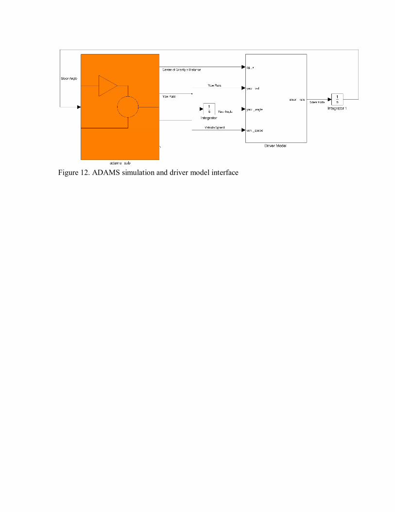
Figure 12. ADAMS simulation and driver model interface

Figure 13. Correlation of Magic Formula driver model to vehicle test at an entry speed of63 km/h

Figure 14. Comparison of different suspension settings and vehicle speeds, for the doublelane change manoeuvre with proposed driver model, where the desired is as proposed byGenta (1997)

Figure 15. Comparison of different suspension settings and vehicle speeds, for thedouble lane change manoeuvre with driver model by Freund and Mayer (1997), wherethe desired is as proposed by Genta (1997)