The Relationship of Sample Size and Accuracy in …...The Relationship of Sample Size and Accuracy in Radial Basis Function Networks HYONTAI SUG Division of Computer and Information

The Relationship of Sample Size and Accuracy in Radial Basis Function Networks

HYONTAI SUG

Division of Computer and Information Engineering Dongseo University

Busan, 617-716 REPUBLIC OF KOREA

[email protected] http://kowon.dongseo.ac.kr/~sht

Abstract: - Even though radial basis function networks are known to have good prediction accuracy in several domains, it is not known to decide a proper sample size like other data mining algorithms, so the task of deciding proper sample sizes for the networks tends to be arbitrary. As the size of samples grows, the improvement in error rates becomes better slowly. But we cannot use larger and larger samples, because we have limited training examples, and there is some fluctuation in accuracy depending on the sample sizes. This paper suggests a progressive resampling technique to cope with the fluction of prediction accuracy values for better radial basis function networks. The suggestion is proved by experiments with promising results. Key-Words: - neural networks, radial basis function networks, sampling

1 Introduction Even though we do not know exactly the reason why a neural network makes a certain forecast, we like neural networks, because their performance in the prediction task is very compatative compared to other data mining or machine learning techniques. So, neural networks are widely used for forecasting tasks like classification and numerical forecasting. Therefore, training neural networks with good accuracy in forecast for a given data set has been a major concern for their success. But even though neural networks are one of the most successful data mining or machine learning methodologies, there are some points of improvement due to the fact that they are built based on greedy algorithms and the knowledge of human experts.

There are two major neural networks that have been applied successfully – multilayer perceptron (MLP) neural networks and radial basis function (RBF) networks. Even though the two networks are similar in shape, their traing mechanisms are very different. MLP neural networks use backpropagation algorithms to train the connection weights so that it takes very long time to train. On the other hand, RBF networks do not perform the backprogagation so that traing time is relatively very short [1, 2].

In order to train connection weights of MLP neural networks the backpropagation algorithms rely on some greedy search algorithms like gradient decent.

Even though the gradient descent works well in most cases, there is still some possibility of considering local optima as global optima [3].

There are many attempts to determine the optimal structures of neural networks based on data [4, 5]. But due to complexity of the methods and specificness of the application domain the structures of the networks are often decided by the knowledge of human experts with some experiments. As a result, built neural networks may not represent the best data mining models that are best for the target domain of the application.

Moreover, because most target databases for data mining are very large, we need sampling process to the target databases. But the task of determining proper sample sizes is arbitrary and the found knowledge based on the random samples is prone to sampling errors or sampling bias.

According to statistics a proper sample size for a feature is 30 or so [6]. For example, to determine the average weight of people, we need to do random sampling for 30 people. But, in general, the target databases of data mining contain a lot of features, so if we do sampling like this, the sample size could become enormous. Moreover, according to experiments using RBF networks the accuracy of the trained RBF networks does not increase monotonically as the sample size grows. So adapting larger and larger sized samples is of no use to find

WSEAS TRANSACTIONS on COMPUTERS Hyontai Sug

ISSN: 1109-2750 1175 Issue 7, Volume 8, July 2009

better RBF networks. Therefore, we need an alternative strategy for sampling.

In section 2, we provide the related work to our research, and in sections 3 we present the background of our method and present the suggested method. Experiments were run to see the effect of the method in section 4. Finally section 5 provides some conclusions.

2 Related Work Neural networks are widely used for machine learning or data mining tasks since the first neural network algorithm, the perceptron [7]. Because of the limited predictability of the perceptron, multilayer perceptrons(MLP) have been invented. In multilayer perceptrons there are two kinds of networks based on how the networks are interconnected – feed-forward neural networks and recurrent neural networks [8]. Radial basis function(RBF) networks are one of the most popular feed-forward networks [9]. Even though RBF networks have three layers including the input layer, hidden layer, and output layer, they differ from a multilayer perceptron, because in RBF networks the hidden layer performs some computation. A good point of RBF networks is that they can be trained in relatively rapid speed. Due to the feed-forward nature and functions in the hidden layer of RBF networks, local optima problem may occur. In order to overcome this problem many evolutionary search algorithms were suggested [10, 11, 12]. Evolutionary search algorithms try to find global optimal solutions based on data so that it is possible to find better RBF networks. But the algorithms require more extensive computing time as well as more elaborate techniques related to the evolutionray computation like the representation technique of the network structures and weights.

Because some induction method is used to train the data mining models like neural networks, the behavior of trained data mining models also dependent on the taining data set. So, there is some research on sample size as well as the property of samples and sampling scheme. Fukunaga and Hayes [13] discussed the effect of sample size for parameter estimates in a family of functions for classifiers. Raudys and Jain [14] prefer small sized samples for feature selection and error estimation for several classifiers for pattern recognition. In [15] the authors showed that class imbalance in training data has effects in neural network development especially for medical domain.

Jensen and Oates [16] investigated three sampling schemes, arithmetic, geometric, and dynamic sampling for decision tree algorithms. In arithmetic sampling and geometric sampling, the sample size grows in arithmetic and geometric manner respectively. Dynamic sampling method determines the sample size based on dynamic programming. They found that the accuracy of predictors increases as the sample size increases and the curve of accuracy is logarithmic, so they used the rate of increase in accuracy as stopping criteria for sampling. In [17] several resampling techniques like cross-validation, the leave-one-out, etc. are tested to see the effect of the sampling techniques in the performance of neural networks, and discovered that the resampling techniques has very different accuracy depending on feature space and sample size.

3 The background of suggested method

3.1 Principles of radial basis function networks Radial basis function networks or RBF networks were introduced in late 80’s. There are many cases that report successful application of RBF networks [18, 19]. The function of RBF networks is based on the function of actual neurons like visual cortices that have the property of being sensitive to some particular visual characteristics [20].

The task of forecasting with RBF network is a classification or regression problem, so the problem can be stated as a function approximation problem. Given a set x of samples (xi, yi) such that f(xi) = yi

for i = 1, ..., n, where n is the sample size and xi is the input vector. We want to find an unknown function f’ that minimize the error, E(f, f’) where f is a prior function that predicts outcome exactly. So, f can be written as follows:

f: I � O (1) where I is the domain of input and O is the domain of output.

Because in the real world situation it is very common to have incomplete training input data set, error estimation is necessary and it is usually done by checking the sum of square of errors E’:

E’ = ∑i=1~n (yi – f’(xi))2 (2)

So, RBF network is a function f’(x) having a linear combination of hidden radial function hj(x). So the RBF network can be written as follows:



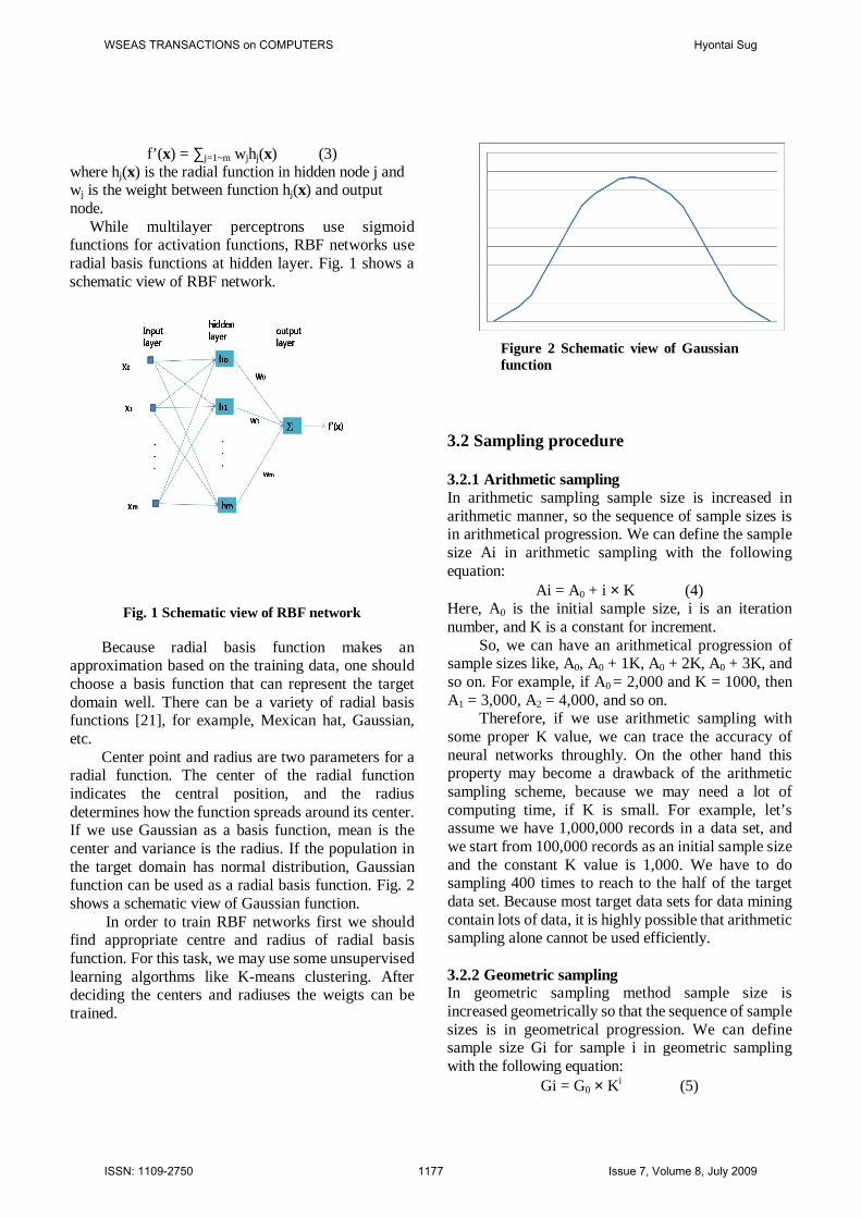
f’( x) = ∑j=1~m wjhj(x) (3) where hj(x) is the radial function in hidden node j and wj is the weight between function hj(x) and output node. While multilayer perceptrons use sigmoid functions for activation functions, RBF networks use radial basis functions at hidden layer. Fig. 1 shows a schematic view of RBF network.

Fig. 1 Schematic view of RBF network

Because radial basis function makes an approximation based on the training data, one should choose a basis function that can represent the target domain well. There can be a variety of radial basis functions [21], for example, Mexican hat, Gaussian, etc.

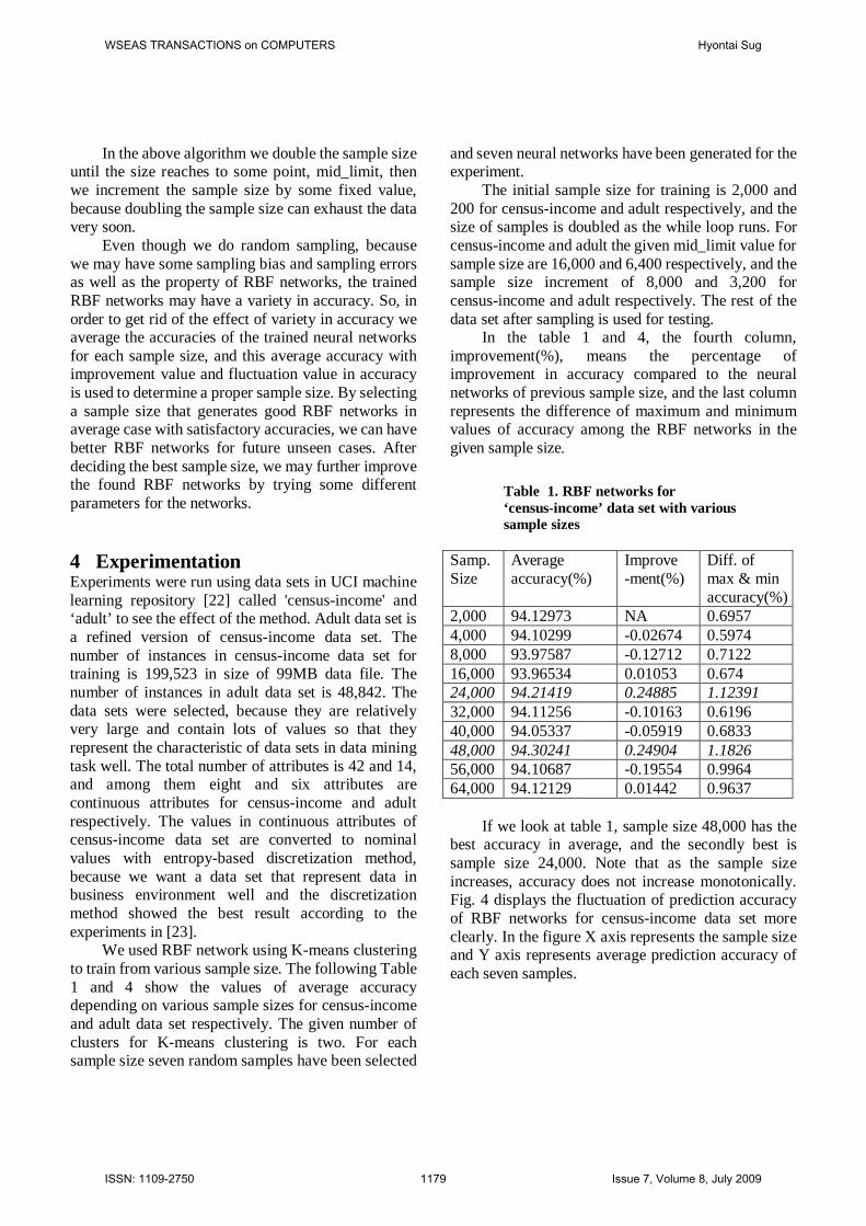
Center point and radius are two parameters for a radial function. The center of the radial function indicates the central position, and the radius determines how the function spreads around its center. If we use Gaussian as a basis function, mean is the center and variance is the radius. If the population in the target domain has normal distribution, Gaussian function can be used as a radial basis function. Fig. 2 shows a schematic view of Gaussian function.

In order to train RBF networks first we should find appropriate centre and radius of radial basis function. For this task, we may use some unsupervised learning algorthms like K-means clustering. After deciding the centers and radiuses the weigts can be trained.

Figure 2 Schematic view of Gaussian function

3.2 Sampling procedure 3.2.1 Arithmetic sampling In arithmetic sampling sample size is increased in arithmetic manner, so the sequence of sample sizes is in arithmetical progression. We can define the sample size Ai in arithmetic sampling with the following equation:

Ai = A0 + i × K (4) Here, A0 is the initial sample size, i is an iteration number, and K is a constant for increment.

So, we can have an arithmetical progression of sample sizes like, A0, A0 + 1K, A0 + 2K, A0 + 3K, and so on. For example, if A0 = 2,000 and K = 1000, then A1 = 3,000, A2 = 4,000, and so on.

Therefore, if we use arithmetic sampling with some proper K value, we can trace the accuracy of neural networks throughly. On the other hand this property may become a drawback of the arithmetic sampling scheme, because we may need a lot of computing time, if K is small. For example, let’s assume we have 1,000,000 records in a data set, and we start from 100,000 records as an initial sample size and the constant K value is 1,000. We have to do sampling 400 times to reach to the half of the target data set. Because most target data sets for data mining contain lots of data, it is highly possible that arithmetic sampling alone cannot be used efficiently. 3.2.2 Geometric sampling In geometric sampling method sample size is increased geometrically so that the sequence of sample sizes is in geometrical progression. We can define sample size Gi for sample i in geometric sampling with the following equation:

Gi = G0 × Ki (5)



Here, G0 is the initial sample size and K is a constant for increment.

So, we can have a geometrical progression of samples in size, G0, G0⋅K, G0⋅K2, G0⋅K3, and so on. For example, if G0 = 2,000 and K = 2, then G1 = 4,000, G2 = 8,000, and so on. As we can see from the example, if we use geometric sampling, sooner or later we can see very big sample sizes. So, the target data set may be exhausted within a few rounds.

As an example, let’s assume that we have 1,000,000 records in a data set as before, and we start from 2,000 records as an initial sample size and the constant K value is 2. So, the sequence of sample size becomes like 2,000, 4,000, 8,000, 16,000, 32,000, 64,000, 128,000, 256,000, 512,000. It takes only 9 rounds to reach to the half of the target data set.

Another noticeable fact in geometric sampling is that the sample size values are very sparse at the later stage of the sampling. So, geometric sampling cannot be a good sampling strategy, if used data mining algorithms do not have the tendency of monotonic increase in accuracy. Let’s assume that we have a learning curve that have some sudden peaks in accuracy as the training size grows. Because geometric sampling method has very sparse sampling interval with respect to sample size at the later stage of the sampling schedule, we might miss the points. Please look at Fig. 3 that depicts learning curve for some induction algorithm. Because there some sudden peaks in accuracy, sparseness in sample sizes may not detect the points.

Fig. 3 Learning curve in accuracy for some possible data mining algorithm

3.3 The method Because we have only limited number of data in the data set and the data set should be divided into two

parts, training and testing, it is not easy to determine an appropriate sample size that is the best for the target data set. In order to overcome this problem we resort to our repeated sampling scheme that considers various sizes of samples to find the best one for the target data set.

We do the sampling until the sample size is less than the half of the target data set, because we assume that we have some large target data set and we want to have enough test data also. The following is a brief description of the procedure of the sampling scheme. ----------------------------------------------------------------------- INPUT : a data set for data mining,

k: the number of random sampling for each sample size,

s: initial sample size. OUTPUT: A, V, I, D. /* A: set of accuracy, V: set of average accuracy, I: set of average improvement D: set of difference in max and min accuracy */ j := 1; Do while s < | target data set | / 2

Do for i = 1 to k /* generate k RBF networks for each loop*/

Do random sampling of size s; Train and test a RBF network; aij := Accuracy of the RBF network; Aj := Aj ∪ {aij};

End for; A := A ∪ Aj; v := the average accuracy in Aj; V := V ∪ {v}; /* V: average accuracy values */ i := (the average accuracy of the RBF networks of

previous step) – ( the average accuracy of the RBF networks); /* average improvement rate */

I := I ∪ { i}; /* I: set of i values */ d := (maximum of accuracy among the trained RBF

networks) - (minimum of accuracy among the trained RBF networks);

/* d stands for the fluctuation of accuracy values in the trained RBF networks */

D := D ∪ {d}; /* D: set of d values */ If s >= mid_limit Then

s := s + sample_size_increment; j++; Else s := s × 2; j++;continue; /* while loop */

End if End while; ---------------------------------------------------------------



In the above algorithm we double the sample size until the size reaches to some point, mid_limit, then we increment the sample size by some fixed value, because doubling the sample size can exhaust the data very soon.

Even though we do random sampling, because we may have some sampling bias and sampling errors as well as the property of RBF networks, the trained RBF networks may have a variety in accuracy. So, in order to get rid of the effect of variety in accuracy we average the accuracies of the trained neural networks for each sample size, and this average accuracy with improvement value and fluctuation value in accuracy is used to determine a proper sample size. By selecting a sample size that generates good RBF networks in average case with satisfactory accuracies, we can have better RBF networks for future unseen cases. After deciding the best sample size, we may further improve the found RBF networks by trying some different parameters for the networks.

4 Experimentation Experiments were run using data sets in UCI machine learning repository [22] called 'census-income' and ‘adult’ to see the effect of the method. Adult data set is a refined version of census-income data set. The number of instances in census-income data set for training is 199,523 in size of 99MB data file. The number of instances in adult data set is 48,842. The data sets were selected, because they are relatively very large and contain lots of values so that they represent the characteristic of data sets in data mining task well. The total number of attributes is 42 and 14, and among them eight and six attributes are continuous attributes for census-income and adult respectively. The values in continuous attributes of census-income data set are converted to nominal values with entropy-based discretization method, because we want a data set that represent data in business environment well and the discretization method showed the best result according to the experiments in [23].

We used RBF network using K-means clustering to train from various sample size. The following Table 1 and 4 show the values of average accuracy depending on various sample sizes for census-income and adult data set respectively. The given number of clusters for K-means clustering is two. For each sample size seven random samples have been selected

and seven neural networks have been generated for the experiment.

The initial sample size for training is 2,000 and 200 for census-income and adult respectively, and the size of samples is doubled as the while loop runs. For census-income and adult the given mid_limit value for sample size are 16,000 and 6,400 respectively, and the sample size increment of 8,000 and 3,200 for census-income and adult respectively. The rest of the data set after sampling is used for testing.

In the table 1 and 4, the fourth column, improvement(%), means the percentage of improvement in accuracy compared to the neural networks of previous sample size, and the last column represents the difference of maximum and minimum values of accuracy among the RBF networks in the given sample size.

Table 1. RBF networks for ‘census-income’ data set with various sample sizes

Samp. Size

Average accuracy(%)

Improve -ment(%)

Diff. of max & min accuracy(%)

2,000 94.12973 NA 0.6957 4,000 94.10299 -0.02674 0.5974 8,000 93.97587 -0.12712 0.7122 16,000 93.96534 0.01053 0.674 24,000 94.21419 0.24885 1.12391 32,000 94.11256 -0.10163 0.6196 40,000 94.05337 -0.05919 0.6833 48,000 94.30241 0.24904 1.1826 56,000 94.10687 -0.19554 0.9964 64,000 94.12129 0.01442 0.9637

If we look at table 1, sample size 48,000 has the

best accuracy in average, and the secondly best is sample size 24,000. Note that as the sample size increases, accuracy does not increase monotonically. Fig. 4 displays the fluctuation of prediction accuracy of RBF networks for census-income data set more clearly. In the figure X axis represents the sample size and Y axis represents average prediction accuracy of each seven samples.



Fig. 4 Fluctuation of average accuracy values of RBF networks for ‘census-income’ data set

Table 2 and table 3 show the details of the experiment for sample size 24,000 and 48,000 for census-income data set respectively.

Table 2 The accuracy of RBF networks for ‘census-income’ data set with sample size 24,000

Sample number Accuracy(%) 1 93.7832 2 94.1808 3 93.8076 4 94.1621 5 93.7768 6 94.7693 7 95.0177

average 94.2142

Table 3 The accuracy of RBF networks for ‘census-income’ data set with sample size 48,000


average 94.3024

The following fig. 5 shows corresponding graph for table 2 data.

Fig. 5 The accuracy of RBF networks for ‘census-income’ data set with sample size 24,000

The following fig. 6 show corresponding graph for table 2 and table 3 data.

The best accuracy in sample size 24,000 is

95.0177% and the best accuracy in sample size 48,000 is 94.9367% so that we may choose one of them as our neural network.

Table 4. RBF networks for ‘adult’ data set with various sample sizes

Samp. size

Average accuracy(%)

Improve -ment(%)

Diff. of max & min accuracy(%)

200 82.15153 NA 2.4239 400 83.3527 1.20117 1.6907 800 82.86174 -0.49096 0.9783 1,600 83.13183 0.27009 1.5071 3,200 83.64977 0.51794 1.1419 6,400 83.38611 -0.26366 2.0288



9,600 83.57734 0.19123 0.6345 12,800 83.45717 -0.12017 0.6165

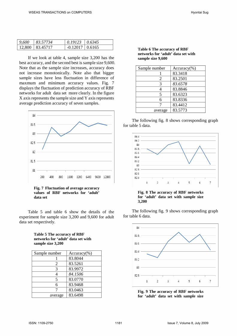
If we look at table 4, sample size 3,200 has the

best accuracy, and the second best is sample size 9,600. Note that as the sample size increases, accuracy does not increase monotonically. Note also that bigger sample sizes have less fluctuation in difference of maxmum and minimum accuracy values. Fig. 7 displays the fluctuation of prediction accuracy of RBF networks for adult data set more clearly. In the figure X axis represents the sample size and Y axis represents average prediction accuracy of seven samples.

Fig. 7 Fluctuation of average accuracy values of RBF networks for ‘adult’ data set

Table 5 and table 6 show the details of the

experiment for sample size 3,200 and 9,600 for adult data set respectively.

Table 5 The accuracy of RBF networks for ‘adult ’ data set with sample size 3,200


average 83.6498

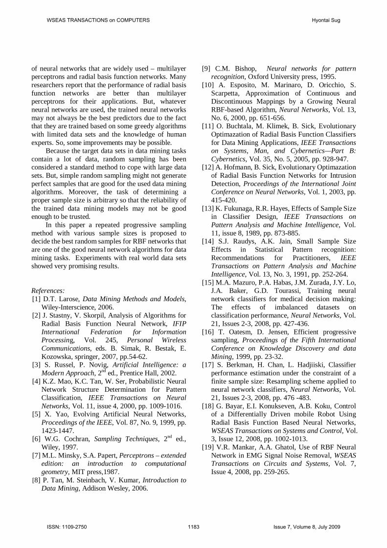
Table 6 The accuracy of RBF networks for ‘adult’ data set with sample size 9,600


average 83.5773 The following fig. 8 shows corresponding graph

for table 5 data.

Fig. 8 The accuracy of RBF networks for ‘adult’ data set with sample size 3,200


Fig. 9 The accuracy of RBF networks for ‘adult’ data set with sample size



9,600

The best accuracy in sample size 3,200 is 84.1506% and the best accuracy in sample size 9,600 is 83.8846% so that we may choose one of them as our neural network.

Finally, in order to see whether we may have better RBF networks, we experimented more with diffrent parameter value for the number of clusters for the sample sizes that have the best average prediction accuracy.Table 7 shows the result for census-income data set with sampel size 48,000. The given number of clusters for K-means clustering is six.

Table 7 The accuracy of RBF networks for ‘census-income’ data set with sample size 48,000 when the number of clusters is six


average 94.4155 If we compare table 3 and table 7, we know that

we obtained the average of 0.1131% improvemet compared to the accuracy of which the number of clusters is two. But the best RBF network was found when the number of cluster is two.


Fig. 10 The accuracy of RBF networks for ‘census-income’ data set with sample size 48,000 when the number of clusters is six

Table 8 shows the result for adult data set with sampel size 3,200. Because adult data set is relatively smaller than census-income data set, the given number of clusters for K-means clustering is four.

Table 8 The accuracy of RBF networks for ‘adult’ data set with sample size 3,200 when the number of clusters is four


average 84.0568 The following fig. 11 shows corresponding graph

for table 7 data.

Fig. 11 The accuracy of RBF networks for ‘adult’ data set with sample size 3,200 when the number of clusters is four

If we compare table 5 and table 8, we know that we obtained the average of 0.4795% improvemet compared to the accuracy of which the number of clusters is two. Moreover, the best one has accuracy of 84.5108%. Note that the best one from two clusters has accuracy of 84.1506%..

5 Conclusions Neural networks are widely accepted for data mining or machine learning tasks so that it is known that neural networks are one of the most successful data mining tools for prediction tasks. There are two kinds



of neural networks that are widely used – multilayer perceptrons and radial basis function networks. Many researchers report that the performance of radial basis function networks are better than multilayer perceptrons for their applications. But, whatever neural networks are used, the trained neural networks may not always be the best predictors due to the fact that they are trained based on some greedy algorithms with limited data sets and the knowledge of human experts. So, some improvements may be possible.

Because the target data sets in data mining tasks contain a lot of data, random sampling has been considered a standard method to cope with large data sets. But, simple random sampling might not generate perfect samples that are good for the used data mining algorithms. Moreover, the task of determining a proper sample size is arbitrary so that the reliability of the trained data mining models may not be good enough to be trusted.

In this paper a repeated progressive sampling method with various sample sizes is proposed to decide the best random samples for RBF networks that are one of the good neural network algorithms for data mining tasks. Experiments with real world data sets showed very promising results. References: [1] D.T. Larose, Data Mining Methods and Models,

Wiley-Interscience, 2006. [2] J. Stastny, V. Skorpil, Analysis of Algorithms for

Radial Basis Function Neural Network, IFIP International Federation for Information Processing, Vol. 245, Personal Wireless Communications, eds. B. Simak, R. Bestak, E. Kozowska, springer, 2007, pp.54-62.

[3] S. Russel, P. Novig, Artificial Intelligence: a Modern Approach, 2nd ed., Prentice Hall, 2002.

[4] K.Z. Mao, K.C. Tan, W. Ser, Probabilistic Neural Network Structure Determination for Pattern Classification, IEEE Transactions on Neural Networks, Vol. 11, issue 4, 2000, pp. 1009-1016.

[5] X. Yao, Evolving Artificial Neural Networks, Proceedings of the IEEE, Vol. 87, No. 9, 1999, pp. 1423-1447.

[6] W.G. Cochran, Sampling Techniques, 2nd ed., Wiley, 1997.

[7] M.L. Minsky, S.A. Papert, Perceptrons – extended edition: an introduction to computational geometry, MIT press,1987.

[8] P. Tan, M. Steinbach, V. Kumar, Introduction to Data Mining, Addison Wesley, 2006.

[9] C.M. Bishop, Neural networks for pattern recognition, Oxford University press, 1995.

[10] A. Esposito, M. Marinaro, D. Oricchio, S. Scarpetta, Approximation of Continuous and Discontinuous Mappings by a Growing Neural RBF-based Algorithm, Neural Networks, Vol. 13, No. 6, 2000, pp. 651-656.

[11] O. Buchtala, M. Klimek, B. Sick, Evolutionary Optimazation of Radial Basis Function Classifiers for Data Mining Applications, IEEE Transactions on Systems, Man, and Cybernetics—Part B: Cybernetics, Vol. 35, No. 5, 2005, pp. 928-947.

[12] A. Hofmann, B. Sick, Evolutionary Optimazation of Radial Basis Function Networks for Intrusion Detection, Proceedings of the International Joint Conference on Neural Networks, Vol. 1, 2003, pp. 415-420.

[13] K. Fukunaga, R.R. Hayes, Effects of Sample Size in Classifier Design, IEEE Transactions on Pattern Analysis and Machine Intelligence, Vol. 11, issue 8, 1989, pp. 873-885.

[14] S.J. Raudys, A.K. Jain, Small Sample Size Effects in Statistical Pattern recognition: Recommendations for Practitioners, IEEE Transactions on Pattern Analysis and Machine Intelligence, Vol. 13, No. 3, 1991, pp. 252-264.

[15] M.A. Mazuro, P.A. Habas, J.M. Zurada, J.Y. Lo, J.A. Baker, G.D. Tourassi, Training neural network classifiers for medical decision making: The effects of imbalanced datasets on classification performance, Neural Networks, Vol. 21, Issues 2-3, 2008, pp. 427-436.

[16] T. Oatesm, D. Jensen, Efficient progressive sampling, Proceedings of the Fifth International Conference on Knowledge Discovery and data Mining, 1999, pp. 23-32.

[17] S. Berkman, H. Chan, L. Hadjiiski, Classifier performance estimation under the constraint of a finite sample size: Resampling scheme applied to neural network classifiers, Neural Networks, Vol. 21, Issues 2-3, 2008, pp. 476 -483.

[18] G. Bayar, E.I. Konukseven, A.B. Koku, Control of a Differentially Driven mobile Robot Using Radial Basis Function Based Neural Networks, WSEAS Transactions on Systems and Control, Vol. 3, Issue 12, 2008, pp. 1002-1013.

[19] V.R. Mankar, A.A. Ghatol, Use of RBF Neural Network in EMG Signal Noise Removal, WSEAS Transactions on Circuits and Systems, Vol. 7, Issue 4, 2008, pp. 259-265.



[20] T. Piggio, F. Girosi, Regularization Algorithms for Learning That are equivalent to Multilayer Networks, Science, Vol. 2247, 1990, pp. 987-982.

[21] Z. Zainuddin, O. Pauline, Function Approximation Using Artificial Neural Networks, WSEAS Transactions on Mathematics, Vol. 7, issue 6, 2008, pp. 333-338.

[22] D. Newman, UCI KDD Archive [http://kdd.ics.uci.edu]. Irvine, CA: University of California, Department of Information and Computer Science, 2005.

[23] Liu, H., Hussain, F., Tan, C.L., Dash, M., Discretization: An Enabling Technique, Data Mining and Knowledge Discovery, Vol. 6, 393-423, 2002.



Documents

The Relationship of Sample Size and Accuracy in …...The Relationship of Sample Size and Accuracy in Radial Basis Function Networks HYONTAI SUG Division of Computer and Information