Embed Size (px)
Citation preview
POUR L'OBTENTION DU GRADE DE DOCTEUR ÈS SCIENCES
PAR
Master of applied science in mechanical engineering, University of Waterloo, Waterloo, Canadade nationalité canadienne
acceptée sur proposition du jury:
Lausanne, EPFL2007
Prof. P. Xirouchakis, président du juryProf. I. Botsis, directeur de thèse
PRof. P. Ermanni, rapporteurProf. R. Salathé, rapporteurProf. A. Vautrin, rapporteur
The response of embedded fbg sensors To non-uniform sTrains in cfrp composiTes during pro-
cessing and delaminaTion
Larissa SORENSEN
THÈSE NO 3710 (2006)
ÉCOLE POLYTECHNIQUE FÉDÉRALE DE LAUSANNE
PRÉSENTÉE LE 20 DÉCEMBRE 2006
à LA FACULTÉ DES SCIENCES ET TECHNIQUES DE L'INGÉNIEUR
Laboratoire de mécanique appliquée et d'analyse de fiabilité
SECTION DE GÉNIE MÉCANIQUE

ii

iii
Acknowledgements
As I finish writing my thesis, I realize how many people motivated, assisted and inspired my work. I must first start by remembering that the door to this thesis opened as I was still trying to close the door on my Master’s thesis. I have Prof. John Botsis to thank for making me an exceptional offer that was definitely worth my crossing the Atlantic. He has given me wonderful opportunities to expand my horizons. I thank him for all the time and effort he has given me as my mentor.
My work has also benefited from close collaboration with Prof. Thomas Gmür. I thank him for his continued support, especially in all areas “numeric”. Dr. Laurent Humbert, provided me with invaluable assistance in matters such as mechanical modelling, optics, and proof-reading. I am very grateful for both his help and friendship.
I would also like to thank the other members of the LMAF laboratory for their assistance, discussion and friendship. In particular, I would like to name Dr. Fabiano Colpo, Gabriel Dunkel, Aleksandar Sekulic, Matteo Galli and Muriel Videlier. Dr. Joël Cugnoni was particularly helpful with regards to material identification tests, digital image correlation and inverse numerical identification methods.
In the early days when I was still getting my feet wet, Dr. Philipe Giaccari was there to show me how to use an OLCR, and how to enjoy a good wine from Valais! Thank-you! Soon after, Dragan Coric arrived – my other optic half. I thank him for all of his help, especially his illuminating explanations and suggestions regarding polarization and birefringence.
I must also thank the students who decided to lend me a hand by dedicating their semester and diploma project work to my cause. Frederic Burri and Gaetan Wicht contributed to the production of specimens and materials testing. Nicolas Amundruz produced the hybrid FBG-Fabry Perot specimens in coordination with the local company ZR-concept. Olivier Compte figured out how to make the hydraulic test machine cooperate and performed preliminary delamination tests. I cannot imagine how all this work would have been accomplished without all of these very capable people. I must also thank the staff of the Atelier – Marc Jeanneret, Gino Crivellari, Nicolas Favre and Stéphane Haldner for their excellent workmanship!
This work would not have been possible without the financial support of the Swiss National Science Foundation and composite material provided by Dr. David Leach of Cytec Industries.
Now, to the people who inspired me and motivated me to come this far, I thank my brother Erik, my extended family and my friends. My mother and father have given me all the support and love a daughter could ask for. I want them both to know how much I appreciate them and how proud I am that they are my parents! Finally, I would like to thank my husband Eric Lumis for supporting my dreams and sharing in the adventures. Without him this would have been a much longer road. How lucky I am to have found such a magnificent partner in life!

v
Abstract
From airplanes to sailboats to bridges, composite materials have become a significant part of our everyday structures. With increasing demand, these materials are pushed to their limits to improve structural efficiency. As a consequence, research and development must continually improve products and provide support for the end user who will need to know the characteristics of their new material. Progress made in the area of optical fibre sensing has opened new avenues for measuring and monitoring fibre-reinforced polymer (FRP) composites, since they can be embedded directly into the composite during manufacturing. These globally noninvasive sensors can provide internal strain and temperature measurements from the moment processing starts until the final failure of the part.
The goal of this research is to develop and demonstrate fibre optic sensing techniques that can characterize the internal strain state of FRP composites. In particular, this work focuses on measuring three-dimensional, non-uniform strain fields in carbon fibre-reinforced polymers (CFRP) using fibre Bragg grating (FBG) sensors. Although FBG sensors are becoming widespread for simple uniaxial strain measurements, their response to complex, non-homogeneous strain fields is still difficult to interpret. To illustrate advances in both experimental techniques and the interpretation of measured FBG data, two main areas of composite monitoring are addressed. They include the study of residual strain evolution and of delamination cracking, which both produce non-homogeneous strain fields.
Unidirectional carbon fibre-reinforced polyphenylene sulphide (AS4/PPS) laminates are observed during processing to measure residual strain progression, and then later subjected to Mode I double cantilever beam delamination tests. These thermoplastic composite specimens are also produced in a cross-ply configuration, for the purpose of residual strain monitoring. In each laminate, a long-gauge length (20-35 mm) FBG is embedded parallel to the reinforcing fibres, and centred along the length of the plate.
Results of polarization sensitive FBG monitoring indicate characteristic material state changes such as the glass-transition and the melting temperatures. These measurements take advantage of both the transverse and longitudinal strain sensitivity of the FBG. When transverse strains are unequal they induce birefringence in the FBG (defining a fast and a slow axis), which results in a split of the normally bell-shaped reflected spectrum. An evolution of this birefringence is monitored during cooling, culminating in average residual transverse strain differences in the embedded FBGs of 230 με and 410 με for unidirectional and cross-ply specimens respectively. Based on the wavelengths measured along the fast polarization axis of the fibre, (observed to be less sensitive to transverse strains) cross-ply specimens exhibit absolute longitudinal residual strains in the order of -350 με. Small longitudinal strain values are the result of the low coefficient of thermal expansion of the carbon reinforcing fibres.
An important step forward in FBG monitoring is taken by measuring the absolute values of the three unequal principal strains in a composite material without making assumptions about the state of strain in the FBG (i.e. diametric loads, plane stress, axisymmetry, etc.). For this purpose, a polarization controlled, hybrid FBG-Fabry Perot optical sensing technique is developed to measure residual strain evolution. The Fabry Perot sensor used in this hybrid method is only sensitive to longitudinal strains, thus providing the additional data required to solve the three-dimensional strain state directly.
vi
To better understand the state of residual strain in the composite material, a temperature dependent thermoelastic finite element model is employed to investigate the strain accumulation during cooling. By comparing modelled results to the data from the optical fibre, it is shown that the mould influences the residual strain development during cooling, and that some of these strains are released after demoulding. Examination of the simulated and experimental curves indicates that the final residual strain state observed with the FBG is close to that of a freely cooling composite plate.
Since the embedded optical fibre is a local inclusion, its strain state is not necessarily that of its host material. In this work, finite element models are used to determine the stresses and strains developed in the surrounding composite material. Near the optical fibre, there is a perturbation of the strain field that extends to a distance of three fibre diameters. In the far-field of cross-ply specimens, tensile transverse stresses reach half the matrix fracture strength. This may help to explain matrix cracking observed on the surface of these specimens.
The second portion of this study is aimed at the measurement of non-uniform longitudinal strains superimposed on an already three-dimensional residual strain state. A polarization adapted optical low coherence reflectometry (OLCR) technique takes distributed measurements of the local Bragg wavelengths for a given polarization axis. For a constant state of birefringence, one can relate the distributed wavelengths to the non-uniform longitudinal strains along the length of the FBG sensor.
Delamination cracking in double cantilever beam specimens creates a non-uniform strain field ideally suited to illustrate this type of measurement. At increasing crack lengths, the distributed wavelengths (proportional to axial strain) are measured by an FBG embedded parallel to the delamination plane. The long gauge length of the sensor provides a sufficiently large set of data so that the crack position and growth direction can be distinguished. The strains retrieved from these experiments are further employed to determine the stress distribution caused by the fibres bridging the delamination crack.
The combination of FBG measurements with inverse identification via finite element modelling is a new technique for determining bridging laws from static delamination specimens. Results of this work indicate that the maximum bridging stress is approximately 2.5 MPa and that the fibre bridging zone length ranges from 20-50 mm. Comparisons of bridging laws determined using this method and a J-integral approach are made using a second finite element model that includes cohesive elements. Simulations of advancing delamination cracks highlight the sensitivity of the force-displacement response of the specimen to differences in bridging laws.
Through the advances in FBG-based methods outlined in this thesis, significant progress is made in the area of non-homogeneous strain detection in fibre-reinforced composites. This allows for improved characterization of three-dimensional residual strain states and the non-uniform strain distributions caused by delamination cracking.
Keywords: fibre Bragg gratings, thermoplastic composites, carbon fibres, polyphenylene sulphide, residual stress, delamination, bridging, birefringence
vii
Version abrégée
Que ce soient les avions, les bateaux ou les ponts, les structures composites font partie de la vie quotidienne. Avec des besoins croissants, ces matériaux sont poussés aux limites pour améliorer l’efficacité des structures. En conséquence, les entreprises doivent continuellement adapter leurs produits et répondre aux besoins des clients qui cherchent à connaître avec précision les caractéristiques des nouveaux matériaux. Comme les senseurs optiques de Bragg (FBGs) peuvent être intégrés directement dans les composites lors de la fabrication, ils suscitent un intérêt croissant pour la mesure et le contrôle des structures composites renforcées. Ces senseurs globalement non invasifs peuvent fournir des informations sur les déformations et la température internes, aussi bien pendant la phase de production qu’au moment de la rupture.
Cette étude a pour but de proposer et développer des techniques de mesure avec des fibres optiques qui permettent la caractérisation de l’état de déformation dans les composites polymères renforcés. En particulier, ce travail s’intéresse à la mesure des déformations tridimensionnelles et non uniformes dans les composites renforcés par des fibres de carbone en utilisant des senseurs de Bragg. Bien que les FBGs soient largement utilisés pour mesurer les déformations uniaxiales, leurs réponses aux champs non homogènes complexes restent toujours difficiles à interpréter. Pour illustrer les avances faites dans les méthodes expérimentales et l’interprétation des données FBG, on étudie dans cette thèse les déformations résiduelles et la délamination dans des composites laminés modèles. Tous les deux produisent des champs de déformation non uniformes.
Des laminés unidirectionnels constitués de polyphenylene sulfide renforcés par des fibres de carbone (AS4/PPS) sont tout d’abord étudiés pendant la phase de production afin de quantifier les déformations résiduelles. Ils sont soumis ensuite à des tests de délamination de type poutre bi-encastrée (mode I). D’autres spécimens sont également fabriqués selon une configuration plis croisés, afin de mesurer les déformations résiduelles. Dans chaque laminé, on insère typiquement un senseur FBG de longueur 20-35-mm parallèlement aux fibres de renfort et à mi-longueur de la plaque.
Les résultats des tests pendant la phase de production montrent que les FBGs peuvent détecter des changements caractéristiques du matériau, tels que la transition vitreuse et la fusion. Cela est possible grâce à la grande sensibilité du senseur aux déformations transverses et axiales. Lorsque les déformations transverses sont différentes, elles induisent de la biréfringence dans le senseur et par conséquent deux axes propres de polarisation (axes lent et rapide) sont à considérer. Le pic de Bragg de la réponse spectrale du FBG se sépare alors en deux. Pendant la phase de refroidissement, on observe une évolution de la biréfringence qui donne lieu à la fin du processus à des différences de déformations transverses de 230 με et 410 με pour les éprouvettes unidirectionnelles et plis croisés, respectivement. Basées sur les longueurs d’onde mesurées le long de l’axe de polarisation rapide, dans ce cas peu sensible aux effets transverses, des déformations longitudinales de l’ordre de -350 με sont enregistrées pour les échantillons plis croisés. Cette valeur assez basse est attribuée au faible coefficient d’expansion thermique des fibres de renfort en carbone.
Une amélioration importante de la méthode de mesure FBG consiste à obtenir des valeurs fiables pour les trois déformations principales dans un composite sans avoir recours à une hypothèse préalable sur l’état de déformation interne. Pour ce faire, on a développé un système hybride FBG-Fabry Perot afin de mesurer les déformations résiduelles, avec un
viii
contrôle de la polarisation. Comme le senseur Fabry Perot est sensible uniquement aux déformations longitudinales, il permet de résoudre complètement les équations opto-mécaniques et d’obtenir les trois composantes de la déformation sans ambigüité.
Afin de mieux comprendre l’état de déformation dans le composite AS4/PPS, on crée un modèle thermoélastique par éléments finis, qui permet de suivre l’évolution des déformations pendant le refroidissement du composite à la fois à l’intérieur et à l’extérieur du moule. En comparant les résultats numériques avec les données expérimentales, on constate que le moule a une influence notable sur les déformations pendant le refroidissement, mais qu’une bonne partie de ces contraintes est relâchée après le démoulage. L’examen des courbes expérimentales et simulées montre qu’au final les déformations dans le FBG sont comparables à celles attendues lorsque le composite se refroidit librement.
Comme la fibre optique est une inclusion, localement les déformations enregistrées ne sont pas forcement celles du matériau environnant. On développe ici un modèle numérique par éléments finis pour déterminer les contraintes et déformations qui se développent dans le composite autour de la fibre. Pour les composites unidirectionnels libres, les contraintes sont proches de zéro tandis que pour les composites à plis croisés elles atteignent la moitié de la résistance de la matrice dans les couches à 90°. On constate une perturbation du champ de déformation à proximité de la fibre optique qui s’étend jusqu’à trois diamètres de fibre.
La deuxième partie de cette étude s’intéresse à la mesure des déformations non uniformes axiales qui se superposent au champ de contraintes résiduelles initial. Une méthode de réflectométrie optique à basse cohérence (OLCR), avec contrôle de polarisation, donne les distributions des longueurs d’onde de Bragg pour chacun des axes de polarisation. Lorsque la biréfringence reste constante, on peut déterminer les déformations non uniformes axiales le long du senseur FBG.
La présence d’une fissure de délamination dans une poutre bi-encastrée engendre un champ non uniforme qui est intéressant pour ce type de mesures. A partir de longueurs de délamination croissantes, on peut mesurer les longueurs d’ondes distribuées (proportionnelles aux déformations axiales) avec un FBG inséré parallèlement au plan de délamination. La longueur du FBG est suffisante pour distinguer la position et la direction de propagation de la fissure.
Les déformations obtenues précédemment peuvent être utilisées pour calculer la distribution de contraintes produites par les fibres pontantes. La combinaison des mesures FBG avec une technique d’identification inverse s’appuyant sur les calculs par éléments finis permet de déterminer une loi de pontage. Les résultats de ce travail indiquent que la contrainte maximale est environ de 2.5 MPa et que la zone de pontage a une longueur de 20 à 40 mm. On propose finalement une comparaison entre la loi de pontage ainsi obtenue et celle qui est prédite par une autre méthode, basée sur l’intégrale J. En implémentant ces lois de pontage dans un second modèle basé sur les éléments cohésifs, on peut alors prédire le comportement global du composite. Les simulations montrent notamment que la courbe force-déplacement de l’échantillon est sensible aux petites variations des paramètres de la loi de pontage.
Grâce aux méthodes de mesure FBG présentées dans cette thèse, un progrès considérable est réalisé dans le domaine de la détection de déformations non homogènes dans les composites polymériques renforcés. Une caractérisation plus précise des déformations résiduelles et des déformations non uniformes causées par les délaminations est ainsi possible.
Mots-clés : senseurs de Bragg, composites thermoplastiques, fibres de carbone, polyphenylene sulfide, contraintes résiduelles, délamination, pontage, biréfringence
ix
Table of Contents
Chapter 1 Introduction...................................................................................................... 1
1.1 Thesis objectives ........................................................................................................ 1 1.2 Thesis organization .................................................................................................... 2
Chapter 2 State of the Art ................................................................................................. 5
2.1 Influence of embedded sensors on composite behaviour .......................................... 5 2.2 Residual strain measurements.................................................................................... 6 2.3 Delamination detection .............................................................................................. 9
Chapter 3 Optical Fibre Sensing .................................................................................... 15
3.1 Description of a fibre Bragg grating ........................................................................ 15 3.2 Spectral amplitude response .................................................................................... 17
3.2.1 Uniform strains along the sensor length .......................................................... 17 3.2.2 Non-uniform strains along the sensor length ................................................... 21 3.2.3 Interpretation of spectra ................................................................................... 22
3.3 Description of hybrid sensing for 3D strain states................................................... 23 3.3.1 Working principles of EFPI sensors ................................................................ 25
3.4 OLCR technique for measuring FBG response ....................................................... 25 3.4.1 Description of OLCR-based system ................................................................ 26 3.4.2 Adaptation of OLCR system for polarization sensitive measurements ........... 28
Chapter 4 Materials and Methods.................................................................................. 31
4.1 Composite plate preparation .................................................................................... 31 4.2 Characterization of AS4/PPS................................................................................... 33
4.2.1 Room temperature elastic properties ............................................................... 35 4.2.2 Temperature dependent elastic properties ....................................................... 36 4.2.3 Coefficients of thermal expansion ................................................................... 37
4.3 Optical fibre characterization................................................................................... 38 4.3.1 Temperature sensitivity.................................................................................... 38 4.3.2 Determination of optomechanical constants .................................................... 38
4.4 Integration of FBG sensors ...................................................................................... 40 4.5 Composite specimens............................................................................................... 42
Chapter 5 Residual Strains ............................................................................................. 45
5.1 Experimental overview ............................................................................................ 45 5.2 Wavelength shifts during processing ....................................................................... 46 5.3 Birefringence as an indication of material state changes during processing ........... 50 5.4 Numerical modelling of residual strains .................................................................. 55
5.4.1 Description of modelling ................................................................................. 55 5.4.2 Explanation of thermoelastic finite element model ......................................... 57 5.4.3 Influence of material properties on simulated Bragg wavelength evolutions.. 60 5.4.4 Comparison of simulated and experimental Bragg wavelength evolutions..... 65 5.4.5 Final stress and strain distributions in the composite ...................................... 67
x
5.5 Discussion of optomechanical relationship simplifications..................................... 73 5.6 Hybrid sensing for 3D residual strain measurement................................................ 74
5.6.1 Specimen description ....................................................................................... 74 5.7 Fibre Bragg grating implementation and response .................................................. 75 5.8 Response of EFPI sensors........................................................................................ 79 5.9 Transverse strains calculated from combined EFPI and FBG data ......................... 79
Chapter 6 Delamination .................................................................................................. 81
6.1 Experimental – DCB testing .................................................................................... 81 6.1.1 Specimen preparation....................................................................................... 81 6.1.2 DCB test procedure.......................................................................................... 83 6.1.3 Mechanical testing results................................................................................ 84 6.1.4 Energy release rate results ............................................................................... 85
6.2 Experimental – FBG measurements ........................................................................ 88 6.2.1 Spectral measurements..................................................................................... 88 6.2.2 OLCR measurements ....................................................................................... 90
6.3 Numerical modelling of DCB specimens ................................................................ 94 6.3.1 Two-dimensional modelling ............................................................................ 95 6.3.2 Three-dimensional modelling .......................................................................... 96 6.3.3 Additional effects on modelling....................................................................... 98
6.4 Numerical identification of bridging stress distributions....................................... 100 6.4.1 Results of optimization .................................................................................. 102 6.4.2 Discussion of results from numerical identification ...................................... 105
6.5 Alternate method for describing bridging.............................................................. 108 6.5.1 Determination of bridging law using J-integral approach ............................. 108 6.5.2 Description of cohesive element behaviour ................................................... 112 6.5.3 Cohesive element modelling.......................................................................... 114
Chapter 7 Conclusions and Perspectives ..................................................................... 119
7.1 Residual strains ...................................................................................................... 119 7.2 Delamination.......................................................................................................... 121 7.3 Perspectives............................................................................................................ 121
References ............................................................................................................................. 123
Appendix A – Silane Preparation....................................................................................... 133
xi
List of Figures
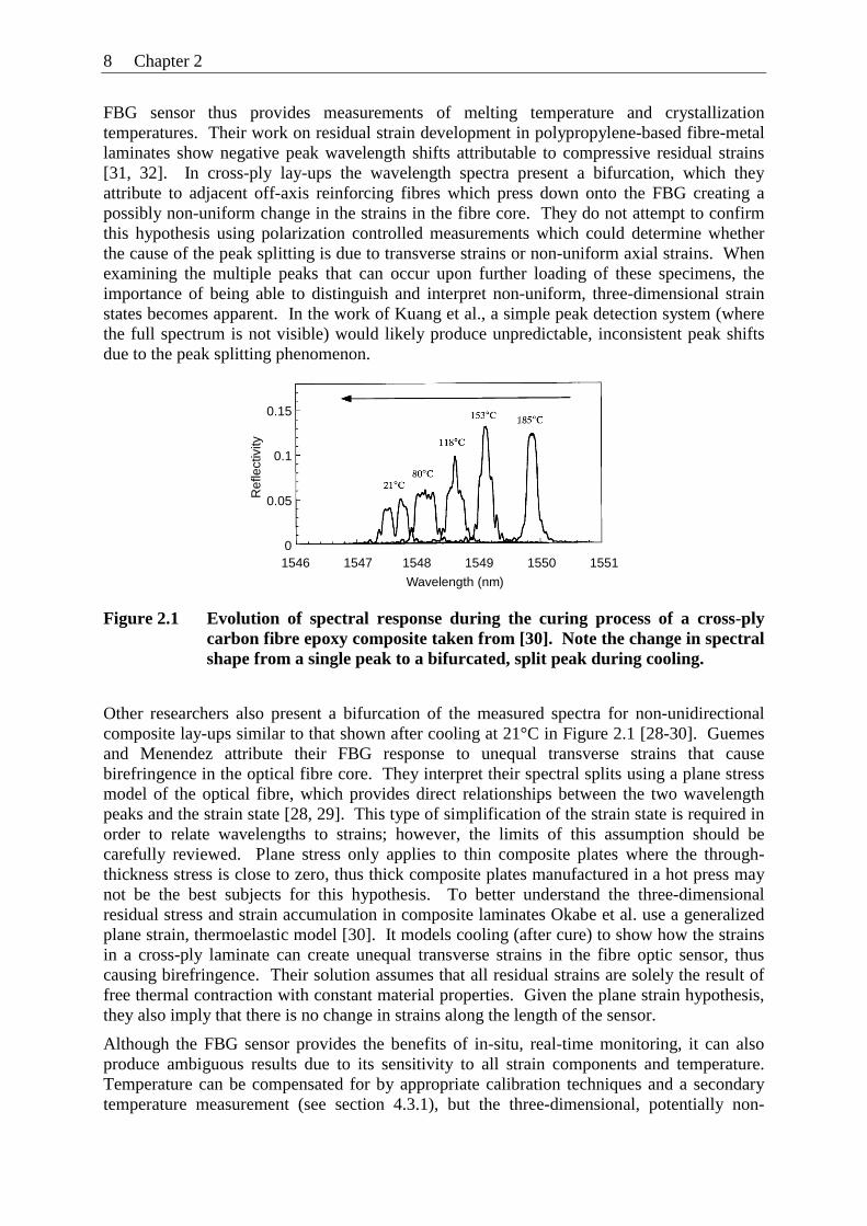
Figure 2.1 Evolution of spectral response during the curing process of a cross-ply carbon fibre epoxy composite taken from [30]. Note the change in spectral shape from a single peak to a bifurcated, split peak during cooling. .................................... 8
Figure 2.2 A 400 KHz air-coupled through-transmission C-scan of solar honeycomb panel with a 5x5-cm stiffener insert from [41]. ......................................................... 10
Figure 2.3 Cohesive laws for different types of material softening, taken from [62]. ...... 12
Figure 3.1 Physical schematic of optical fibre with typical dimensions for single mode fibres used in this study. ................................................................................... 15
Figure 3.2 Profiles of refractive index modulations for (a) a homogeneous grating, and (b)
a chirped grating, with a period defined by)(
2zz θπ +
Λ . ................................. 16
Figure 3.3 Schematic of a free FBG with a constant grating pitch Λ. When broadband light I(λ) is injected into the FBG its original spectral amplitude wavelength peak λB can be defined by either the reflection R(λ) or transmission T(λ) responses. ......................................................................................................... 17
Figure 3.4 Illustration of spectral measurements for the FBG response to unequal transverse strains .............................................................................................. 19
Figure 3.5 Example of peak split observed when light is injected into an FBG with strain-induced birefringence. Here light is injected at an angle of about 45° to the principal strain/optical axes.............................................................................. 20
Figure 3.6 Spectrum taken from the work of Studer et al. showing the response to non-uniform axial strains caused by debonding [75]. ............................................. 21
Figure 3.7 Example of spectral response for an embedded FBG subjected to a distributed longitudinal strain field εz(z) caused by a delamination crack. ........................ 22
Figure 3.8 Hybrid optical fibre measurement system........................................................ 24
Figure 3.9 EFPI sensor schematic ..................................................................................... 25
Figure 3.10 Simplified schematic of OLCR-based measurement system constructed by P. Giaccari. A more detailed schematic can be found in [70]. ............................ 26
Figure 3.11 a) Impulse amplitude measurement of 22 mm long FBG sensor, b) reflection spectrum and c) reconstructed local Bragg wavelengths along the length of the sensor, where the sensor entrance is found at a position of 1.5 mm. ............... 27
Figure 3.12 Measurements of phase φ (z) in an unembedded FBG grating. ....................... 27
Figure 3.13 Measurements of local Bragg wavelength for the sensor from Figure 3.12. Measurements are taken with two different mirror step sizes and starting at both ends of the sensor (forwards and backwards). ......................................... 28
Figure 3.14 Schematic of polarization adapted OLCR system, including additional polarization control. OLCR based on [70]. ..................................................... 29
xii
Figure 3.15 Impulse amplitude response when a) light is aligned along an axis (or no birefringence), and b) when light is injected at about 45° in a birefringent specimen. The distance between minima is half the beat length. ................... 29
Figure 4.1 a) Pre-preg plies stacked in steel mould. b) Mould in hot-press (plastic release film prevents sticking to top platen)................................................................. 31
Figure 4.2 Processing temperature and pressure cycle for AS4/PPS laminates ................ 32
Figure 4.3 Micrographs showing fibre distribution at a) low, and b) high magnifications [93]. The low-magnification photo indicates little separation between plies with a nominal thickness of 130 mm........................................................................ 33
Figure 4.4 Storage moduli (E22) from DMTA tests compared to E22 from tensile tests.... 36
Figure 4.5 Coefficient of thermal expansion as a function of temperature T. ................... 37
Figure 4.6 a) Diametric loading setup and b) loading diagram of optical fibre for analytical calculations ...................................................................................... 39
Figure 4.7 Slow and fast axis measurements of wavelength peak position with increasing diametric load ................................................................................................... 39
Figure 4.8 a) Top view of composite plate lay-up and b) cross-sectional view of plate in the mould.......................................................................................................... 41
Figure 4.9 a) Distribution of carbon fibres around a 125 μm diameter fibre optic sensor and b) distribution of fibres and plies around FBG in a cross-ply laminate .... 42
Figure 5.1 Schematic for data acquisition during processing............................................ 46
Figure 5.2 Comparison of raw wavelength measurements (no temperature correction) with the measured temperature profile ..................................................................... 47
Figure 5.3 Changes in wavelength (temperature corrected) during processing for a typical unidirectional specimen (specimen 10)............................................................ 47
Figure 5.4 Measurements from both slow and fast axes, where the left (fast axis) peak is less sensitive to the initial hot press loading (specimen 26)............................. 48
Figure 5.5 Comparison of normalized relative displacement between mould top and bottom compared to wavelength shifts from unidirectional specimens ........... 49
Figure 5.6 Temperature corrected wavelength shifts during cooling, with the reference state taken at Tc ................................................................................................ 50
Figure 5.7 Evolution of reflected spectra during the heating portion of plate production. (uncorrected for temperature shift, specimen 32) ............................................ 51
Figure 5.8 Evolution of reflected spectra during the cooling portion of plate production. (uncorrected for temperature shift, specimen 32) ............................................ 52
Figure 5.9 Final spectral response, measured for each of the polarization axes. The separation between the two peaks indicates the residual birefringence (specimen 32). .................................................................................................. 53
Figure 5.10 Measurements of peak splits (λbx-λby) with respect to temperature during cooling. Depending on the arbitrary polarization state during processing, some specimens only have measurements obtained after processing........................ 53
Figure 5.11 Spectral response for both fast and slow polarization axes (specimen 26) ...... 54
xiii
Figure 5.12 OLCR measurements of local Bragg wavelength for an embedded FBG sensor measured on each of the principal polarization axes. These measurements are compared to the original, non-birefringent measurement (specimen 26). ....... 55
Figure 5.13 Schematic of embedded optical fibre in an infinite host, where the reinforcing fibres of the host and the optical fibre are aligned in the z-direction. A uniform temperature field ΔT is applied. ....................................................................... 56
Figure 5.14 Schematics showing sectional views of boundary conditions for the a) unconstrained and b) constrained cases ........................................................... 57
Figure 5.15 Example of meshing near the optical fibre for the cross-ply configuration. Boundaries between plies and around the optical fibre are indicated by bold lines. ................................................................................................................. 58
Figure 5.16 Mesh for the unconstrained cross-ply specimen fibre showing a close-up in the area around the optical fibre............................................................................. 58
Figure 5.17 Discritization of the matrix dependent material properties E22 and α22 for the incremental model. ........................................................................................... 60
Figure 5.18 Results from parametric studies for constrained and unconstrained unidirectional specimens .................................................................................. 62
Figure 5.19 Results from parametric studies for cross-ply constrained and unconstrained specimens ......................................................................................................... 63
Figure 5.20 Wavelength shifts for the rightmost peak in a unidirectional specimen during cooling. Numerical and experimental results are compared. .......................... 64
Figure 5.21 Wavelength shifts for the rightmost peak in a cross-ply specimen during cooling. Numerical and experimental results are compared. .......................... 64
Figure 5.22 Strains in the optical fibre, as calculated by the unconstrained (dark lines) and constrained (light lines) models ....................................................................... 65
Figure 5.23 Birefringence evolution as described by peak splitting. Numerical calculations of peak split (solid lines) are compared to experimental results (filled points: unidirectional, outlined points: cross-ply)........................................................ 66
Figure 5.24 Final residual stresses calculated along the y-axis (through-thickness) in the unidirectional specimen, where a) represents the unconstrained case and b) represents the constrained case. ....................................................................... 68
Figure 5.25 Final residual stresses calculated along the y-axis (through-thickness) in the cross-ply specimen, where a) represents the unconstrained case and b) represents the constrained case. ....................................................................... 69
Figure 5.26 Final residual strains calculated along the y-axis (through-thickness) in the unidirectional specimen, where a) represents the unconstrained case and b) represents the constrained case. ....................................................................... 70
Figure 5.27 Final residual strains calculated along the y-axis (through-thickness) in the cross-ply specimen, where a) represents the unconstrained case and b) represents the constrained case. ....................................................................... 71
Figure 5.28 Error caused by using the pe relationship to calculate axial strains from wavelength, where case studies come from the four numerical models used in the previous section .......................................................................................... 73
xiv
Figure 5.29 a) Composite block in mould. b) Cross-section of specimen indicating actual positions of optical sensors and thermocouple................................................. 75
Figure 5.30 Change in wavelength response of an embedded FBG during cooling. Due to the lack of polarization control, the peak measurement varies periodically. ... 76
Figure 5.31 Polarization controlled spectral measurements using a tuneable laser ............ 77
Figure 5.32 Effect of optimized polarization rotation (18°/s) on measured wavelength response from the Micron Optics interrogator. Maximums and minimums represent the slow and fast axes respectively................................................... 77
Figure 5.33 Measurements taken with rotating polarization, with different alignments of the injected light are compared for their accuracy when measuring peak split. .... 78
Figure 5.34 Evolution of FBG wavelengths during cooling (referenced at 80°C). ............. 78
Figure 5.35 Increase in longitudinal strain measured by EFPI sensors during cooling ...... 80
Figure 5.36 Evolution of transverse strains during cooling determined using EFPI and FBG data. .................................................................................................................. 80
Figure 6.1 Delamination specimen showing the placement of the thermocouple, FBG, pre-crack and 5mm scale ........................................................................................ 82
Figure 6.2 Schematic of 200 mm long DCB specimen indicating the opening displacement Δ, measured load P, FBG location, thickness 2h = 3.7 mm, pre-crack length a0 = 60-70 mm, distance from load to crack tip a, distance from load to end of specimen l = 5 mm, location of z-coordinate axis............................................ 82
Figure 6.3 Set-up for delamination testing in hydraulic test machine. .............................. 83
Figure 6.4 Digital image capture of the crack tip progression (specimen 32)................... 84
Figure 6.5 Force-displacement measurements for DCB specimens with (thick lines) and without (thin lines) embedded FBG sensors .................................................... 85
Figure 6.6 Example of fibre bridging for a long delamination crack length ..................... 85
Figure 6.7 Evolution of elastic strain energy release rate for all DCB specimens ............ 87
Figure 6.8 a) Schematic of a longitudinal strain (εz) distribution in an FBG embedded at a distance of 0.26 mm parallel to the delamination plane as shown in insert b) Actual spectral distribution measured for a given crack length in specimen 28........................................................................................................................... 89
Figure 6.9 Comparison of spectral measurements for specimen 32. Black lines represent polarizations aligned close to the fast axis and the grey lines those aligned close to the slow axis........................................................................................ 90
Figure 6.10 OLCR amplitude measurement showing relative location of FBG sensor and the end of the optical fibre................................................................................ 90
Figure 6.11 Measurements of local Bragg wavelength shift relative to initial embedded wavelength for three crack lengths in specimen 32 ......................................... 91
Figure 6.12 Specimen 26 wavelength shift measurements for increasing crack lengths are numbered from 1 to 4. The corresponding visually measured crack tip positions are indicated with arrows. ................................................................. 92
xv
Figure 6.13 Specimen 31 wavelength shift measurements for increasing crack lengths are numbered from 1 to 3. The corresponding visually measured crack tip positions are indicated with arrows. ................................................................. 93
Figure 6.14 Specimen 32 wavelength shift measurements for increasing crack lengths are numbered from 1 to 5. The corresponding visually measured crack tip positions are indicated with arrows. ................................................................. 93
Figure 6.15 Specimen 28 wavelength shift measurements for six crack lengths, taken when the cracks are held open at half the maximum displacement ........................... 94
Figure 6.16 Final configuration of plane strain finite element model. ................................ 95
Figure 6.17 Radial mesh refinement at the crack tip with quadratic elements.................... 95
Figure 6.18 Experimental (specimen 32) and FE axial strain distributions. 2D and 3D simulations are plotted. .................................................................................... 96
Figure 6.19 Convergence study showing longitudinal strain distributions for different types and sizes of elements........................................................................................ 97
Figure 6.20 Three-dimensional FE model showing boundary conditions, coarse global mesh and submodel section mesh .................................................................... 98
Figure 6.21 Comparison of the effect of 2D and 3D models on the calculated wavelength shift (specimen 32) ........................................................................................... 99
Figure 6.22 Flowchart of inverse identification procedure ............................................... 100
Figure 6.23 Evolution of longitudinal strain distributions and corresponding bridging stress parameters during the optimization procedure............................................... 103
Figure 6.24 a) Bridging stress distributions for specimen 26 and b) experimental strain distributions (thin black lines) vs. output from optimized numerical model . 104
Figure 6.25 a) Bridging stress distributions for specimen 31 and b) experimental strain distributions (thin black lines) vs. output from optimized numerical model . 104
Figure 6.26 a) Bridging stress distributions for specimen 32 and b) experimental strain distributions (thin black lines) vs. output from optimized numerical model. Due to the variation in the experimental data, three curve fits are used for the “long” crack: min., avg., and max.................................................................. 105
Figure 6.27 Photograph of bridging fibres for specimen 31 showing transition between high and low densities of bridging fibres (The crack-tip is beyond the frame of the photo.) ............................................................................................................ 106
Figure 6.28 For the model including an optimization of an applied moment: a) bridging stress distributions for specimen 32 and b) experimental strain distributions (thin black lines) vs. output from optimized numerical model. Due to the variation in the experimental data, two curve fits are used for the “long” crack: min., and avg. ................................................................................................. 109
Figure 6.29 Schematic of fibre bridging across the delamination crack, where a0 is the pre-crack length, a is the crack length, δ is the crack separation, Δ is the applied opening displacement and z is the distance from the crack tip..................... 110
Figure 6.30 a) Measured mode I energy release rate (GI) with curve fits and b) calculated bridging stress distributions. Grey represents the non-equilibrium state and black represents the equilibrium state. ........................................................... 111
xvi
Figure 6.31 Comparison of bridging laws determined using the J-integral for both the equilibrium and non-equilibrium cases and using the FBG-inverse identification technique. These curves represent specimen 32. .................... 112
Figure 6.32 a) Schematic of a cohesive element submitted to opening displacement δ. b) Basic cohesive law describing the constitutive response of the element ....... 113
Figure 6.33 Definition of the constitutive behaviour of a cohesive element modified for fibre bridging, based on [56] .......................................................................... 114
Figure 6.34 Cohesive element model ................................................................................ 115
Figure 6.35 Force displacement response for specimen 32 compared with results from cohesive element models one and two. .......................................................... 116
Figure 6.36 Force displacement response for specimen 32 compared with results from cohesive element models three and four. ....................................................... 117
Figure 6.37 Comparison of experimental axial strains from the FBG with strains obtained by cohesive modelling and optimized pressure distribution modelling......... 118

xvii
List of Tables
Table 4.1 Room temperature properties for AS4/PPS [0]28 from tests and from manufacturer [96]. ............................................................................................ 36
Table 4.2 Longitudinal (α11) and transverse (α22) coefficients of thermal expansion at room temperature ............................................................................................. 38
Table 4.3 Mechanical and optical properties for the FBG optical fibre sensor................ 40
Table 4.4 List of AS4/PPS specimen configurations ....................................................... 43
Table 5.1 Average values of peak split and transverse strain difference for unidirectional and cross-ply plates .......................................................................................... 54
Table 5.2 Temperature independent material properties for the glass optical fibre and steel mould ....................................................................................................... 59
Table 5.3 Initial composite property values at room temperature used for FEM modelling.......................................................................................................................... 61
Table 5.4 Composite property values at room temperature used for final FEM model configuration .................................................................................................... 62
Table 5.5 Summary of stresses and strains calculated with numerical models................ 72
Table 6.1 Strain energy release rate initiation values GIC determined using two methods.......................................................................................................................... 87
Table 6.2 Limits on parameters used in Equation 6.9. ................................................... 101
Table 6.3 Forces on the loading pin determined from models run with optimized bridging stress distributions .......................................................................................... 106
Table 6.4 Results of study on the specimen 31 model comparing the force on the loading pins for different crack lengths....................................................................... 107
Table 6.5 Total bridging strain energy release rates calculated for specimen 32........... 112
Table 6.6 Parameters defining the initial constitutive response of the cohesive elements........................................................................................................................ 114

Chapter 1 Introduction
Laminated polymer composites provide excellent structural performance and versatility due to our ability to tailor-design their properties. They can be manufactured for applications requiring high specific strength or stiffness. Composites can also be designed for applications requiring chemical resistance or high temperature functionality. Due to the multitude of possible configurations, fibre-reinforced polymers have found an equally abundant number of uses from the mundane to the extraordinary. It must therefore be the aim of researchers to determine pertinent methods for ensuring quality production, accurate characterization, and reliable health monitoring of critical composite structures. Progress in this area is complicated by the heterogeneous nature that defines a composite material. Parts made of two or more distinct phases (i.e. fibres and matrix), with anisotropic properties and multiple layers of different orientations, are clearly difficult to fully characterize.
Consider the description of the production process and its influence on the residual stresses and strains in a material. If one can monitor the build-up of strains during fabrication then one may be able to detect the parameters that affect these strains. An improvement of the process could reduce part warpage and spring-back or reduce internal stresses that may be detrimental to the residual strength of the composite. Moreover, the determination of residual stresses permits a more realistic evaluation of a material’s resistance to further loading.
Ideally a material could be followed from production to service, with a means for monitoring strain evolution and distribution. The same sensor could not only measure residual strains, but in-service damage such as delamination. It is important to provide global, real-time measurement of delamination, since this type of damage can be initiated at any time due to a dropped tool or an impact with debris or even a pebble. An in-situ sensor for continuous monitoring that does not require extensive, heavy cabling, and does not require an interruption of service would be favourable. Herein lays a niche for fibre optic sensors that can be embedded directly into a real composite structure. Being internal sensors, fibre optics can also “see” composites in a new way: from the inside-out. This viewpoint should be exploited when evaluating the potential of these sensors to monitor residual stresses and damage.
1.1 Thesis objectives
This work focuses on developing an understanding of the response of embedded optical fibre sensors to the internal strain state of carbon fibre-reinforced polymer (CFRP) composites. Specifically, this work is interested in fibre Bragg grating (FBG) sensors and their reaction to real world strains that are present due to manufacturing or damage. For mechanical engineers to properly apply these sensors for strain-monitoring, they must fully understand the sensitivity of an FBG to strain states that are not simply uniaxial, but three-dimensional (3D) and non-uniform. This understanding is critical for the development of pertinent experimental and numerical techniques described in this thesis. Applications of FBG sensing
2 Chapter 1
in non-uniform strain fields are exemplified by the following two areas common to composite materials research: residual strains and delamination.
The novelty of this work can be summarized by the implementation and interpretation of FBG sensors to provide multi-dimensional and distributed measurements. In particular, we:
• measure characteristic temperatures for material state changes in a thermoplastic laminate during processing with FBG sensors that are sensitivie to unequal transverse strains. An examination of the complete 3D strain field via the sensor response also provides insight into the influence of the mould on the development of residual stresses.
• improve on the measurement of 3D, residual strain fields, by incorporating hybrid sensing (FBG and Fabry Perot optical sensors) with rotating polarization control of the injected light. Using this spectrally-based sensing technique, all three principal strains are determined experimentally without recourse to a two-dimensional assumption such as plane stress in the composite.
• adapt the in-house developed optical low-coherence reflectometry (OLCR) unit for polarization controlled measurements in composites with unequal transverse strains. Using this newly configured arrangement, the OLCR technique can be applied to measure strains that are not only unequal in the transverse direction, but also distributed along the length of the sensor. This is the state of strain that develops due to the progression of a delamination crack. With a single FBG sensor this method can determine crack growth direction and location.
• combine the FBG strain measurements with iterative finite element modelling to identify the distribution of bridging fibre tractions across the delamination crack plane. This method calculates a bridging law without needing to assume that the crack propagates in a self-similar manner or that a single point can describe the entire bridging zone.
1.2 Thesis organization
This thesis is organized into four main areas: background, materials and methods, residual strains and delamination.
Following this introduction, Chapter 2 describes the benefits of FBG sensors and explains how they can influence the composite material in which they are embedded. Methods for residual stress and delamination detection using both classical means and FBG sensors are discussed to give the reader an overview of current techniques, along with their benefits and limitations.
Next, Chapter 3 focuses directly on the background required to understand the optical response of an FBG to mechanically applied strains. In this chapter the mathematical relationships between strain and wavelength are developed for cases ranging from constant axial strains to non-homogeneous, distributed strains. The application of the OLCR for non-uniform longitudinal strain sensing is discussed, along with the adaptations necessary for measurements in unequal transverse strain fields. At the end of this chapter, a brief introduction of Fabry Perot optical sensors is intended to support the understanding of the hybrid optical sensing technique.
Introduction 3
Chapter 4 provides characteristic information about the carbon fibre reinforced polyphenylene sulphide composite and the FBG sensors used in residual stress and delamination testing. It gives details of the composite production method and of the optical fibre embedding technique. Results of tests for composite and optical fibre properties are elaborated upon in this section.
Chapters 5 contains the contribution on residual strain measurements and modelling. It presents the use of FBG sensing for determining residual strain development in a thermoplastic composite due to processing. Spectral measurements highlight changes in spectral shape (peak split) that can be related to changes in material state. Peak split, caused by unequal transverse strains, is confirmed using the new polarization controlled OLCR technique. The development of residual strains is modelled using finite elements to determine the correlation between three dimensional strains and observed wavelength shifts. It is also used to evaluate the far-field stresses in the composite material, which are different from those in the optical fibre inclusion. Based on this modelling it is clear that it would be beneficial to develop a purely experimental technique for obtaining the 3D strains in the FBG. This is the motivation for the development of a hybrid technique using polarization controlled measurements of FBG and Fabry Perot optical sensors. The Fabry Perot sensor is only sensitive to axial strains, whereas the FBG is sensitive to all three principal strains. By embedding both into a thick carbon fibre-reinforced epoxy specimen, it is possible to extract all three strains experimentally.
Chapter 6 focuses on non-uniform longitudinal strain distributions resulting from delamination cracking. In studies of delaminations in double cantilever beam specimens the polarization adapted OLCR is used to follow the wavelength distribution along the length of a long FBG sensor, which can be related directly to the distribution of axial strains. These strain distributions are then input into an inverse identification model to extract the distribution of bridging tractions across the delaminated fracture plane. Cohesive element modelling is then employed to compare the effects of bridging distributions obtained with an alternate experimental technique and with the FBG method.
Finally, Chapter 7 concludes this thesis by highlighting the main achievements of this work. It also provides perspectives regarding possible avenues for future development in this area of research.


Chapter 2 State of the Art
The advent of optical fibre sensing has created many new opportunities for measurement and sensing. Early on in their development, simple optical fibres are embedded into structures to detect damage by observing the failure of the sensors themselves. If the sensor is damaged, it leaks light and then the intensity of the light passing transmitted at the end of the fibre is decreased [1]. Advances in photosensitivity [2] lead to the development of a fibre Bragg grating (FBG) sensor that both academia and industry are quick to adopt. This type of sensor has many benefits such as [3]:
• non-intrusive size (typically 125 μm diameter)
• extremely low sensitivity to electromagnetic interference
• good resistance to corrosion
• large capacity for multiplexing (reducing wiring needed for strain gauges)
• high temperature capacity
• long working lifetime (> 25 years)
• excellent sensitivity to strain and temperature
• signal is wavelength encoded
For these reasons FBG sensors are being implemented in many fields to detect temperature and/or strain. Various fields already benefit from FBG sensing, including: civil structural engineering, the electrical power industry, marine and aerospace vehicles, and medicine [3]. Due to their geometry, these sensors are also particularly well suited to being embedded in fibre-reinforced polymer (FRP) composite structures. Hence, there exists a growing area of research into FBG sensors for process monitoring, health monitoring, or damage detection in “smart-structures” fabricated with composite materials. Researchers generally measure the reflected wavelength peak shift from the sensor and relate this directly to the applied axial strain. The following sections discuss the reliability of FRP composites instrumented with embedded optical fibres. They also describe the areas of residual strain and delamination detection with respect to current practices and optical fibre sensing.
2.1 Influence of embedded sensors on composite behaviour
The effect of embedded optical fibres on the strength, stiffness and fatigue life of composite specimens is an important consideration for those using sensors for long-term monitoring. This topic is the subject of some research; however, as explained by Jensen et al. [4], investigations indicate sometimes contradictory results ranging from improvement, to slight degradation in mechanical performance of composites containing embedded sensors [1, 4-8].
6 Chapter 2
When examining the data one must keep in mind that this type of testing is predisposed to the inherent scatter involved when producing and testing composite materials. The laminate lay-up, the number of embedded sensors and their type of coating (bare fibre, acrylate coating etc.) may also influence the results.
Despite these discrepancies, an overall tendency indicates that the inclusion of a single FBG causes little, or no strength/stiffness degradation in tension when embedded parallel to the reinforcing fibres [4-6]. Alignment with the reinforcing fibres is preferred, as it causes the least amount of perturbation of the surrounding fibres. This may be especially true in compression testing, where fibres embedded perpendicular to the reinforcing fibres and perpendicular to the loading direction cause up to 70% reduction in strength [7]. It is also shown that fibre orientation is important in bending, where a specimen with an OF embedded off-axis in a 0/45 interface causes about 50% reduction in bending strength compared to a specimen with sensors embedded parallel to reinforcing fibres [8].
In fatigue, the results are as varied as in static tests. The origins of crack initiation and orientation may be attributed to the optical fibres [6] or to normal delamination starting at the edges of the specimen [9]. Some tests show decrease in fatigue lives [6] and others show no noticeable changes [9, 10]. Although more work is required to determine the various parameters that can affect these test results, the current research is nevertheless significant. It highlights the need to treat the optical fibre as an inclusion that must be considered as being more or less intrusive depending on the embedding conditions.
2.2 Residual strain measurements
Residual stresses and strains are those that remain in a material after fabrication, processing or some other event. They can be beneficial, like those induced in the production of tempered glass, or they can be detrimental, like those that cause problems in dimensional tolerances, create warping, or provoke premature failure. In certain cases, transverse cracking may occur in a composite simply due to residual strains [11, 12].
Polymer composites are subject to significant residual stresses and strains due to their anisotropic and non-homogeneous nature [13, 14]. Strains are induced by shrinkage from polymerization, crystallization and thermal dilatation. Mismatches in coefficients of thermal expansion of the component materials cause residual strains on a microscopic level, while thermal expansion mismatch between plies of different orientations produces a similar effect on a laminar scale. On a global laminate level, strains may vary throughout a laminate due to tool-part interaction or thermal gradients. The total residual strain field in a composite material is the combination of all of these effects.
There exist various methods for following the development of residual strains during processing, or for determining their magnitude after fabrication. One can embed resistance strain gauges into the composite to measure strain evolution during processing [14, 15]. This works well for low temperature processes in sample specimens where the intrusiveness of the gauges and wiring will not cause later concerns. Measurements obtained during processing may enable one to determine the origin of certain residual stresses. For example, Kim and Daniel are able to evaluate the significance of part-tool interaction during resin transfer moulding [14]. Using both strain gauges (and extrinsic Fabry Perot interferometric sensors in parallel), a large jump in strains (over 5000 μm) is observed in the reinforcing fibre direction after the demoulding of a unidirectional CFRP from an aluminium mould. This returns the
State of the Art 7
strain state to a value close to that of the strain induced at maximum process temperature, which is attributed to the initial thermal expansion of the mould.
The most common methods for measuring residual stresses in FRP composites take advantage of dimensional instability or curvature of a laminate. Often this involves the fabrication of asymmetric laminates that will warp after consolidation [11, 13, 14, 16]. The curvature of these plates is related to the residual stresses caused by thermal contraction/curing of the anisotropic plies at various orientations. In the case of a two layer composite one can calculate the residual stresses based on a modified bi-metallic strip model [11, 13]. For more involved lay-ups, curvature and stresses are calculated analytically using classical laminate theory [16]. When the calculated curvature matches the measured curvature, it is assumed that the calculated residual stresses are accurate. Researchers note that the calculations of residual stresses are dependent on the material properties (stiffness, coefficient of thermal expansion, etc.) which are themselves dependent on temperature. In the production of thermoplastics, where processing temperatures are often elevated, it may be important to calculate stress evolution in steps, taking into account the appropriate material properties for a given temperature.
Symmetric laminates do not undergo warpage; however, researchers may use a destructive layer removal technique to remove outer plies, thereby artificially creating an asymmetric laminate for which curvature or outer-ply strain can be measured [16, 17]. Although this technique provides curvature, it may be difficult to accurately control the removal of a given number of plies, and may leave an uneven surface. To improve upon this idea, another method (Process Simulated Laminate) uses thin layers of release film between designated plies, creating easily removable layers [18, 19]. When each group of plies is removed, strains are measured using a strain gauge mounted on the opposite side of the laminate. This is effective even in the case of a unidirectional laminate where global residual stresses may occur due to thermal gradients in specimens during cooling.
Some of the other techniques available for residual strain measurement include the compliance method [17], hole-drilling[20], moiré interferometry [21, 22], Raman spectroscopy [23] and X-ray diffraction [24]. These methods range from the destructive to the non-destructive, and require increasingly complex equipment and procedures for their implementation. In the case of X-ray diffraction, only crystalline polymers or polymers filled with crystalline particles can be examined.
Clearly the door is open for innovative measurement techniques that are non-destructive, non-intrusive, portable and life-long. Optical fibre sensors can fill this role, providing in-situ data during processing, after processing and during service. Efforts are currently being made to fill this need using methods based on FBG sensors to measure strains during and after processing.
Numerous studies consider the responses of fibre Bragg gratings to the accumulation of residual strains in composite materials. Most often, research focuses on monitoring the curing of thermosetting resins and composites where residual strains are the result of matrix shrinkage during polymerization and thermal shrinkage during cooling [14, 25-30]. After subtracting temperature effects, results from these studies generally show that the FBG spectral peaks translate towards decreased wavelengths, indicating compressive residual longitudinal strains.
Much less work exists in the area of thermoplastic composites. Kuang et al. have studied the processing of fibre-metal laminate and sandwich composites with a polypropylene matrix [31-33]. They observe the development of strains throughout processing, and are able to determine transitions in material state based on changes in peak wavelength shift [33]. The
8 Chapter 2
FBG sensor thus provides measurements of melting temperature and crystallization temperatures. Their work on residual strain development in polypropylene-based fibre-metal laminates show negative peak wavelength shifts attributable to compressive residual strains [31, 32]. In cross-ply lay-ups the wavelength spectra present a bifurcation, which they attribute to adjacent off-axis reinforcing fibres which press down onto the FBG creating a possibly non-uniform change in the strains in the fibre core. They do not attempt to confirm this hypothesis using polarization controlled measurements which could determine whether the cause of the peak splitting is due to transverse strains or non-uniform axial strains. When examining the multiple peaks that can occur upon further loading of these specimens, the importance of being able to distinguish and interpret non-uniform, three-dimensional strain states becomes apparent. In the work of Kuang et al., a simple peak detection system (where the full spectrum is not visible) would likely produce unpredictable, inconsistent peak shifts due to the peak splitting phenomenon.
1546 1547 1548 1549 1550 1551
0.15
0.1
0.05
0
Wavelength (nm)
Ref
lect
ivity
Figure 2.1 Evolution of spectral response during the curing process of a cross-ply carbon fibre epoxy composite taken from [30]. Note the change in spectral shape from a single peak to a bifurcated, split peak during cooling.
Other researchers also present a bifurcation of the measured spectra for non-unidirectional composite lay-ups similar to that shown after cooling at 21°C in Figure 2.1 [28-30]. Guemes and Menendez attribute their FBG response to unequal transverse strains that cause birefringence in the optical fibre core. They interpret their spectral splits using a plane stress model of the optical fibre, which provides direct relationships between the two wavelength peaks and the strain state [28, 29]. This type of simplification of the strain state is required in order to relate wavelengths to strains; however, the limits of this assumption should be carefully reviewed. Plane stress only applies to thin composite plates where the through-thickness stress is close to zero, thus thick composite plates manufactured in a hot press may not be the best subjects for this hypothesis. To better understand the three-dimensional residual stress and strain accumulation in composite laminates Okabe et al. use a generalized plane strain, thermoelastic model [30]. It models cooling (after cure) to show how the strains in a cross-ply laminate can create unequal transverse strains in the fibre optic sensor, thus causing birefringence. Their solution assumes that all residual strains are solely the result of free thermal contraction with constant material properties. Given the plane strain hypothesis, they also imply that there is no change in strains along the length of the sensor.
Although the FBG sensor provides the benefits of in-situ, real-time monitoring, it can also produce ambiguous results due to its sensitivity to all strain components and temperature. Temperature can be compensated for by appropriate calibration techniques and a secondary temperature measurement (see section 4.3.1), but the three-dimensional, potentially non-
State of the Art 9
uniform, strain field can cause difficulties in the interpretation of the sensor response. Moreover, Kollár and Van Steenkiste remind us that the FBG is an inclusion in the composite, and that its strains and stresses are not necessarily those of the surrounding host material [34]. Pertinent models, (which can be complicated by the moulding procedure and composite lay-up) are required to equate optical fibre strains to those in the far-field composite.
Many authors rely on thermoelastic models to determine the stress-strain fields accumulated during the consolidation of a thermoplastic composite. They are able to calculate stresses for multi-ply, multi-directional composites based on classical laminate theory [16, 35]. They stress the importance of separating the cooling process into appropriate temperature steps, so that the incremental stresses (strains) are representative of the material properties in that step. For example, above the glass-transition temperature Tg matrix moduli are low, so that less stress is accumulated than in an equivalent temperature step below Tg. At the end of the cooling process, the final stresses are calculated to be the sum of all those calculated in the individual steps.
With finite element modelling one can implement generalized plane strain models to calculate incremental strains (stress) [22, 36]. Here again authors are careful to incorporate temperature-dependent material properties. In this way, appropriate stress fields are calculated without the need to move to more complicated viscoelastic models. Depending on the polymer, one may also include temperature dependent factors such as changes in crystallinity into the residual strain calculations [22]. Crystallinity will change the effective matrix modulus and will cause additional shrinkage. The importance of this effect is not well defined when one examines the results of studies that incorporate or neglect this effect [13, 37, 38].
The advantages of incorporating thermoviscoelasticity instead of an incremental thermoelastic model are also unclear. Concerns with thermoelastic approaches rise from the potential to overestimate internal residual stresses since they ignore relaxation [39]. However, the process of accurately measuring the parameters that define an orthotropic composite’s viscoelastic behaviour is complicated. It is also difficult to find commercially available finite element code that deals with anisotropic thermovisoelastic behaviour, therefore requiring the development of user-subroutines or in-house finite element code. In an examination of the literature concerning thermoplastic composites it appears that previously referenced thermoelastic models (with appropriately incremented thermal steps) can produce equally valid results in comparison to viscoelastic models [38-40].
2.3 Delamination detection
Delamination is one of the major failure mechanisms in laminated composites. Often starting at an edge or between plies, delamination can occur due to many types of loading: fatigue, impact or others. Interlaminar failure of this type can be difficult to observe, since often there is no visual clue or external crack to give warning, making this type of damage very dangerous in critical structures such as aircraft. Although structures can be designed to be damage resistant, it is still important to be able to perform periodic inspections which can detect internal damage. Herein lays the challenge of delamination detection: one must generally use an external method to find internal flaws. Techniques such as radiography, ultrasonics and thermography all provide solutions to this problem [41, 42].
Radiography, better known as X-rays, traditionally provides two-dimensional images of composite parts. This type of image requires expert interpretation and strict safety measures
10 Chapter 2
due to the health hazard associated with the ionizing radiation. Progress has been made in the field of computer imaging so that radiography now includes the technique best known for its medical applications: the CT scan. Computed tomography (CT) scans are produced by using a computer to interpret the distribution of the X-ray transmission intensities in a structure for multiple viewing angles [41, 43]. A CT scan furnishes information about the distribution of the density of a material, hence, it can show areas of voids, or material separation where delamination has occurred. A CT scan may even be performed to produce three-dimensional analysis of a material.
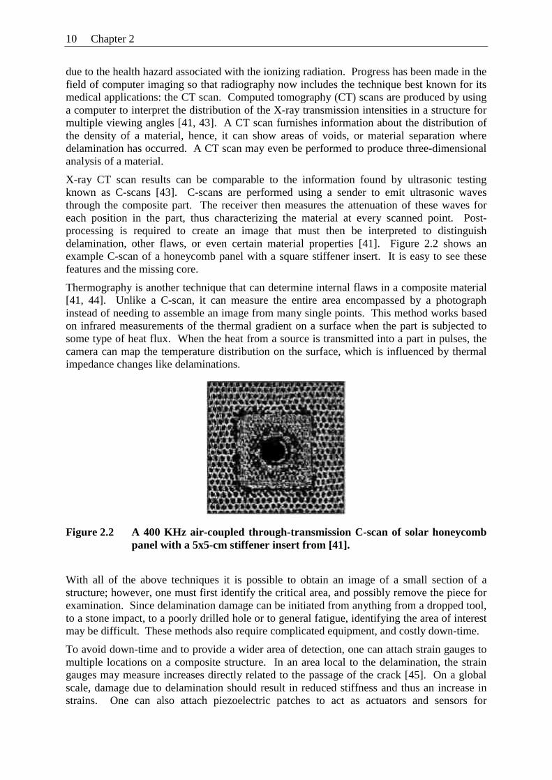
X-ray CT scan results can be comparable to the information found by ultrasonic testing known as C-scans [43]. C-scans are performed using a sender to emit ultrasonic waves through the composite part. The receiver then measures the attenuation of these waves for each position in the part, thus characterizing the material at every scanned point. Post-processing is required to create an image that must then be interpreted to distinguish delamination, other flaws, or even certain material properties [41]. Figure 2.2 shows an example C-scan of a honeycomb panel with a square stiffener insert. It is easy to see these features and the missing core.
Thermography is another technique that can determine internal flaws in a composite material [41, 44]. Unlike a C-scan, it can measure the entire area encompassed by a photograph instead of needing to assemble an image from many single points. This method works based on infrared measurements of the thermal gradient on a surface when the part is subjected to some type of heat flux. When the heat from a source is transmitted into a part in pulses, the camera can map the temperature distribution on the surface, which is influenced by thermal impedance changes like delaminations.
Figure 2.2 A 400 KHz air-coupled through-transmission C-scan of solar honeycomb panel with a 5x5-cm stiffener insert from [41].
With all of the above techniques it is possible to obtain an image of a small section of a structure; however, one must first identify the critical area, and possibly remove the piece for examination. Since delamination damage can be initiated from anything from a dropped tool, to a stone impact, to a poorly drilled hole or to general fatigue, identifying the area of interest may be difficult. These methods also require complicated equipment, and costly down-time.
To avoid down-time and to provide a wider area of detection, one can attach strain gauges to multiple locations on a composite structure. In an area local to the delamination, the strain gauges may measure increases directly related to the passage of the crack [45]. On a global scale, damage due to delamination should result in reduced stiffness and thus an increase in strains. One can also attach piezoelectric patches to act as actuators and sensors for
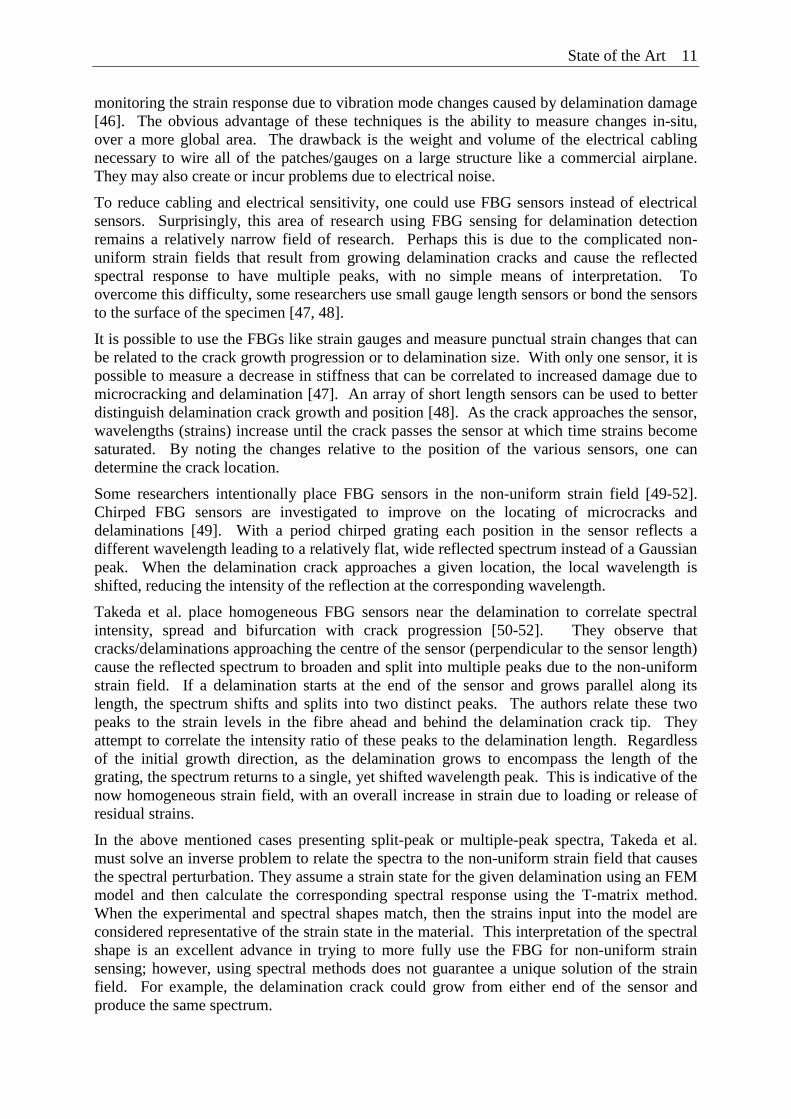
State of the Art 11
monitoring the strain response due to vibration mode changes caused by delamination damage [46]. The obvious advantage of these techniques is the ability to measure changes in-situ, over a more global area. The drawback is the weight and volume of the electrical cabling necessary to wire all of the patches/gauges on a large structure like a commercial airplane. They may also create or incur problems due to electrical noise.
To reduce cabling and electrical sensitivity, one could use FBG sensors instead of electrical sensors. Surprisingly, this area of research using FBG sensing for delamination detection remains a relatively narrow field of research. Perhaps this is due to the complicated non-uniform strain fields that result from growing delamination cracks and cause the reflected spectral response to have multiple peaks, with no simple means of interpretation. To overcome this difficulty, some researchers use small gauge length sensors or bond the sensors to the surface of the specimen [47, 48].
It is possible to use the FBGs like strain gauges and measure punctual strain changes that can be related to the crack growth progression or to delamination size. With only one sensor, it is possible to measure a decrease in stiffness that can be correlated to increased damage due to microcracking and delamination [47]. An array of short length sensors can be used to better distinguish delamination crack growth and position [48]. As the crack approaches the sensor, wavelengths (strains) increase until the crack passes the sensor at which time strains become saturated. By noting the changes relative to the position of the various sensors, one can determine the crack location.
Some researchers intentionally place FBG sensors in the non-uniform strain field [49-52]. Chirped FBG sensors are investigated to improve on the locating of microcracks and delaminations [49]. With a period chirped grating each position in the sensor reflects a different wavelength leading to a relatively flat, wide reflected spectrum instead of a Gaussian peak. When the delamination crack approaches a given location, the local wavelength is shifted, reducing the intensity of the reflection at the corresponding wavelength.
Takeda et al. place homogeneous FBG sensors near the delamination to correlate spectral intensity, spread and bifurcation with crack progression [50-52]. They observe that cracks/delaminations approaching the centre of the sensor (perpendicular to the sensor length) cause the reflected spectrum to broaden and split into multiple peaks due to the non-uniform strain field. If a delamination starts at the end of the sensor and grows parallel along its length, the spectrum shifts and splits into two distinct peaks. The authors relate these two peaks to the strain levels in the fibre ahead and behind the delamination crack tip. They attempt to correlate the intensity ratio of these peaks to the delamination length. Regardless of the initial growth direction, as the delamination grows to encompass the length of the grating, the spectrum returns to a single, yet shifted wavelength peak. This is indicative of the now homogeneous strain field, with an overall increase in strain due to loading or release of residual strains.
In the above mentioned cases presenting split-peak or multiple-peak spectra, Takeda et al. must solve an inverse problem to relate the spectra to the non-uniform strain field that causes the spectral perturbation. They assume a strain state for the given delamination using an FEM model and then calculate the corresponding spectral response using the T-matrix method. When the experimental and spectral shapes match, then the strains input into the model are considered representative of the strain state in the material. This interpretation of the spectral shape is an excellent advance in trying to more fully use the FBG for non-uniform strain sensing; however, using spectral methods does not guarantee a unique solution of the strain field. For example, the delamination crack could grow from either end of the sensor and produce the same spectrum.
12 Chapter 2
Imagine now that a delamination crack has been detected. How does one predict the remaining lifetime of the part? For simple cracks and geometry, linear elastic fracture mechanics provides solutions for estimating the severity of the crack. The severity is given by the stress intensity factor K which can, for example, be related to remaining fatigue life [53]. In more complicated structures or composite lay-ups, a simple calculation may not be adequate. Moreover, composites may display crack bridging (fibres crossing the open crack) which will change the behaviour of the delamination. In this case it is useful to both find material characterization methods that can correctly describe the delamination behaviour, and to find appropriate methods for modelling complex delamination scenarios.
Recent studies are approaching this problem by using advances in interfacial cohesive element modelling [54-57]. To correctly predict the behaviour of a delamination crack one must first have a good understanding of the parameters describing crack progression, specifically, the strain energy release rate G. However, researchers show that resistance of a composite G(δ) with crack opening δ is found to be dependent on test geometry due to the phenomenon of fibre bridging [56, 58]. To better describe the influence of bridging fibres, authors use the concept of a cohesive zone based on the work by Dugdale and Barenblatt [59, 60], and first applied to the study of concrete cracking by Hillerborg [61]. This zone is described by a softening (cohesive) law that relates the decrease in bridging stresses σb to crack opening δ. Figure 2.3, taken from Crisfield et al., regroups various types of cohesive laws [62]. Here, the area under the curve is equal to the strain energy release rate.
Figure 2.3 Cohesive laws for different types of material softening, taken from [62].
When implementing cohesive element modelling one clearly requires an accurate cohesive law in order to produce pertinent results. Often the law takes on an assumed shape, for example linear or exponential as in the above figure. Some researchers [56, 63] try to determine the exact law by measuring the mode I strain energy release rate GI = JI [64] and crack opening displacement δ* at the pre-crack tip in a double cantilever beam specimen, which can then be correlated to the bridging stresses σb via:
This method is relatively simple to execute; however it is difficult to determine the final value of δ* relating to zero cohesive/bridging stress, which can be critical in crack growth predictions (see Chapter 6 for further description). It also assumes that the crack propagates in a self-similar manner and that a single point can describe the entire bridging zone.
*)( *d
dGI δσδ b= ( 2.1 )

State of the Art 13
The determination of bridging stresses across delamination cracks remains an open area of research, where new measurement methods are required. Very little data exists on the measurement of delamination bridging stresses. Given the potential of new in-house developments for measuring non-uniform strains using optical low-coherence reflectometry [25, 65], it is reasonable to consider FBG sensing as an alternative for both delamination sensing and characterization. With an embedded FBG sensor, one can take advantage of an internal, distributed strain measurement to describe the crack location, growth direction and the bridging zone.

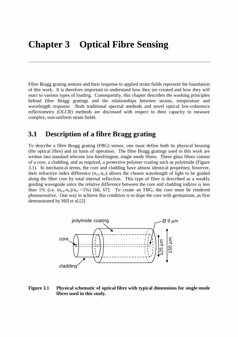
Chapter 3 Optical Fibre Sensing
Fibre Bragg grating sensors and their response to applied strain fields represent the foundation of this work. It is therefore important to understand how they are created and how they will react to various types of loading. Consequently, this chapter describes the working principles behind fibre Bragg gratings and the relationships between strains, temperature and wavelength response. Both traditional spectral methods and novel optical low-coherence reflectometry (OLCR) methods are discussed with respect to their capacity to measure complex, non-uniform strain fields.
3.1 Description of a fibre Bragg grating
To describe a fibre Bragg grating (FBG) sensor, one must define both its physical housing (the optical fibre) and its basis of operation. The fibre Bragg gratings used in this work are written into standard telecom low-birefringent, single mode fibres. These glass fibres consist of a core, a cladding, and as required, a protective polymer coating such as polyimide (Figure 3.1). In mechanical terms, the core and cladding have almost identical properties; however, their refractive index difference (nco-ncl) allows the chosen wavelength of light to be guided along the fibre core by total internal reflection. This type of fibre is described as a weakly guiding waveguide since the relative difference between the core and cladding indices is less than 1% (i.e. (nco-ncl)/ncl <1%) [66, 67]. To create an FBG, the core must be rendered photosensitive. One way to achieve this condition is to dope the core with germanium, as first demonstrated by Hill et al.[2].
Figure 3.1 Physical schematic of optical fibre with typical dimensions for single mode fibres used in this study.
150
μm
125
μm
Ø 9 μm polyimide coating
cladding
core
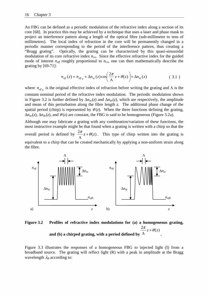
16 Chapter 3
An FBG can be defined as a periodic modulation of the refractive index along a section of its core [68]. In practice this may be achieved by a technique that uses a laser and phase mask to project an interference pattern along a length of the optical fibre (sub-millimetre to tens of millimetres). The local index of refraction in the core will be permanently changed in a periodic manner corresponding to the period of the interference pattern, thus creating a “Bragg grating”. Optically, the grating can be characterized by this quasi-sinusoidal modulation of its core refractive index nco. Since the effective refractive index for the guided mode of interest neff roughly proportional to nco, one can then mathematically describe the grating by [69-71]:
where 0effn is the original effective index of refraction before writing the grating and Λ is the
constant nominal period of the refractive index modulation. The periodic modulation shown in Figure 3.2 is further defined by Δnac(z) and Δndc(z), which are respectively, the amplitude and mean of this perturbation along the fibre length z. The additional phase change of the spatial period (chirp) is represented by θ (z). When the three functions defining the grating, Δnac(z), Δndc(z), and θ (z) are constant, the FBG is said to be homogeneous (Figure 3.2a).
Although one may fabricate a grating with any combination/variation of these functions, the most instructive example might be that found when a grating is written with a chirp so that the
overall period is defined by )(2
zz θπ +Λ
. This type of chirp written into the grating is
equivalent to a chirp that can be created mechanically by applying a non-uniform strain along the fibre.
Figure 3.2 Profiles of refractive index modulations for (a) a homogeneous grating,
and (b) a chirped grating, with a period defined by)(
2zz θπ +
Λ .
Figure 3.3 illustrates the responses of a homogeneous FBG to injected light (I) from a broadband source. The grating will reflect light (R) with a peak in amplitude at the Bragg wavelength λB according to:
)()(2
cos)()(0
znzzznnzn dcaceffeff Δ+⎟⎠⎞
⎜⎝⎛ +
ΛΔ+= θπ
( 3.1 )
Δnac
Δndc
neff0
z
neff
Λ
Δnac
Δndc
neff0
z
neff
Λ
b) a)
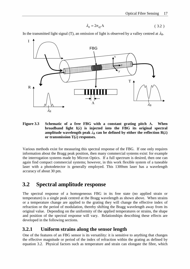
Optical Fibre Sensing 17
In the transmitted light signal (T), an omission of light is observed by a valley centred at λB.
Figure 3.3 Schematic of a free FBG with a constant grating pitch Λ. When broadband light I(λ) is injected into the FBG its original spectral amplitude wavelength peak λB can be defined by either the reflection R(λ) or transmission T(λ) responses.
Various methods exist for measuring this spectral response of the FBG. If one only requires information about the Bragg peak position, then many commercial systems exist: for example the interrogation systems made by Micron Optics. If a full spectrum is desired, then one can again find compact commercial systems; however, in this work flexible system of a tuneable laser with a photodetector is generally employed. This 1300nm laser has a wavelength accuracy of about 30 pm.
3.2 Spectral amplitude response
The spectral response of a homogeneous FBG in its free state (no applied strain or temperature) is a single peak centred at the Bragg wavelength as shown above. When strains or a temperature change are applied to the grating they will change the effective index of refraction or the period of modulation, thereby shifting the Bragg wavelength away from its original value. Depending on the uniformity of the applied temperatures or strains, the shape and position of the spectral response will vary. Relationships describing these effects are developed in the following sections.
3.2.1 Uniform strains along the sensor length One of the features of an FBG sensor is its versatility: it is sensitive to anything that changes the effective magnitude or period of the index of refraction within the grating as defined by equation 3.2. Physical factors such as temperature and strain can elongate the fibre, which
Λ= effB n2λ ( 3.2 )
λB
R
I
T
λB
FBG
Λ
y
z
x
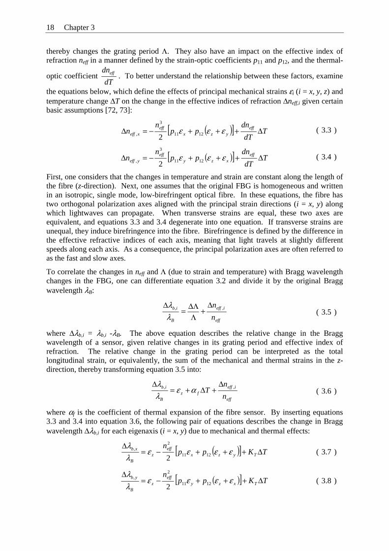
18 Chapter 3
thereby changes the grating period Λ. They also have an impact on the effective index of refraction neff in a manner defined by the strain-optic coefficients p11 and p12, and the thermal-
optic coefficient dT
dneff . To better understand the relationship between these factors, examine
the equations below, which define the effects of principal mechanical strains εi (i = x, y, z) and temperature change ΔT on the change in the effective indices of refraction Δneff,i given certain basic assumptions [72, 73]:
First, one considers that the changes in temperature and strain are constant along the length of the fibre (z-direction). Next, one assumes that the original FBG is homogeneous and written in an isotropic, single mode, low-birefringent optical fibre. In these equations, the fibre has two orthogonal polarization axes aligned with the principal strain directions (i = x, y) along which lightwaves can propagate. When transverse strains are equal, these two axes are equivalent, and equations 3.3 and 3.4 degenerate into one equation. If transverse strains are unequal, they induce birefringence into the fibre. Birefringence is defined by the difference in the effective refractive indices of each axis, meaning that light travels at slightly different speeds along each axis. As a consequence, the principal polarization axes are often referred to as the fast and slow axes.
To correlate the changes in neff and Λ (due to strain and temperature) with Bragg wavelength changes in the FBG, one can differentiate equation 3.2 and divide it by the original Bragg wavelength λB:
where Δλb,i = λb,i -λB. The above equation describes the relative change in the Bragg wavelength of a sensor, given relative changes in its grating period and effective index of refraction. The relative change in the grating period can be interpreted as the total longitudinal strain, or equivalently, the sum of the mechanical and thermal strains in the z-direction, thereby transforming equation 3.5 into:
where αf is the coefficient of thermal expansion of the fibre sensor. By inserting equations 3.3 and 3.4 into equation 3.6, the following pair of equations describes the change in Bragg wavelength Δλb,i for each eigenaxis (i = x, y) due to mechanical and thermal effects:
( )[ ] TdT
dnpp
nn eff
yzxeff
xeff Δ+++−=Δ εεε 1211
3
, 2 ( 3.3 )
( )[ ] TdT
dnpp
nn eff
xzyeff
yeff Δ+++−=Δ εεε 1211
3
, 2 ( 3.4 )
eff
ieff
B
ib
n
n ,, Δ+
ΛΔΛ=
Δλλ
( 3.5 )
eff
iefffz
B
ib
n
nT ,, Δ
+Δ+=Δ
αελλ
( 3.6 )
( )[ ] TKppn
Tyzxeff
zB
xb Δ+++−=Δ
εεεελλ
1211
2,
2 ( 3.7 )
( )[ ] TKppn
Txzyeff
zB
yb Δ+++−=Δ
εεεελλ
1211
2,
2 ( 3.8 )
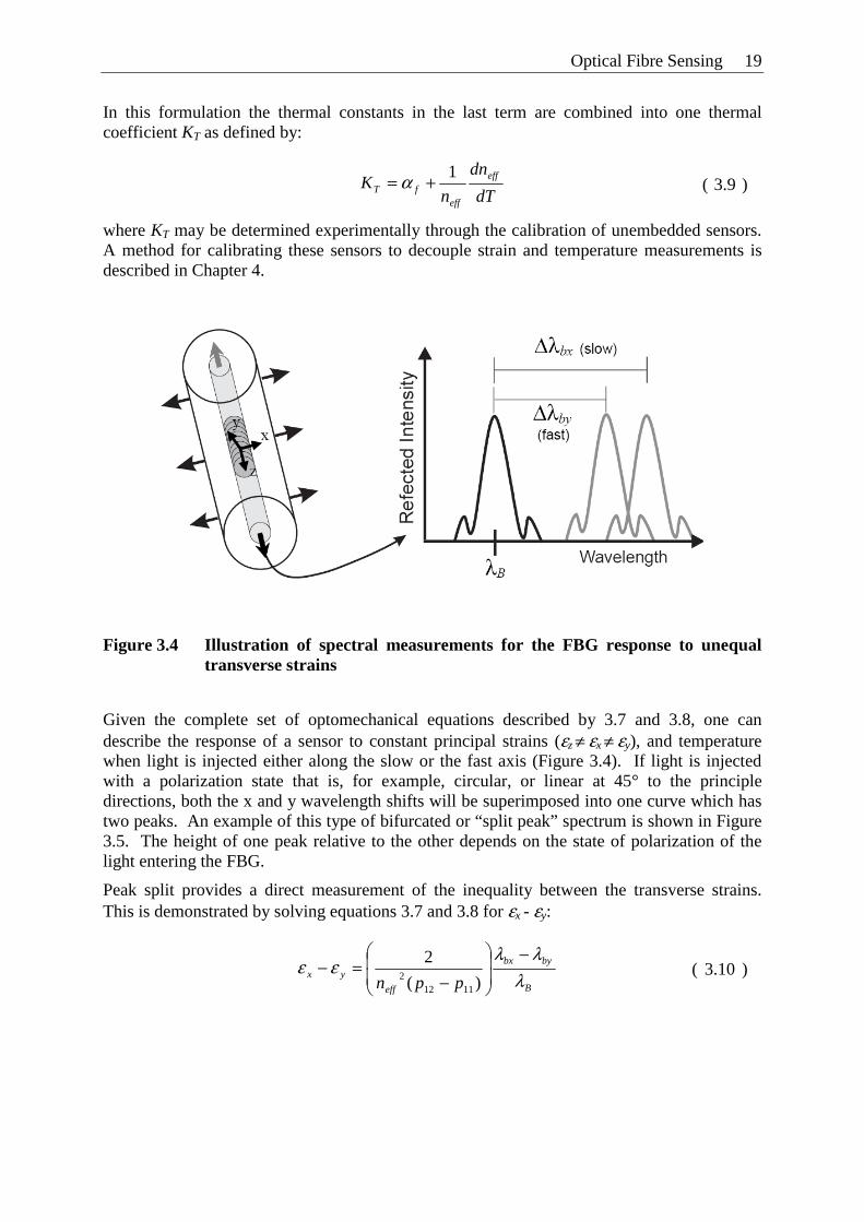
Optical Fibre Sensing 19
In this formulation the thermal constants in the last term are combined into one thermal coefficient KT as defined by:
where KT may be determined experimentally through the calibration of unembedded sensors. A method for calibrating these sensors to decouple strain and temperature measurements is described in Chapter 4.
Figure 3.4 Illustration of spectral measurements for the FBG response to unequal transverse strains
Given the complete set of optomechanical equations described by 3.7 and 3.8, one can describe the response of a sensor to constant principal strains (εz ≠ εx ≠ εy), and temperature when light is injected either along the slow or the fast axis (Figure 3.4). If light is injected with a polarization state that is, for example, circular, or linear at 45° to the principle directions, both the x and y wavelength shifts will be superimposed into one curve which has two peaks. An example of this type of bifurcated or “split peak” spectrum is shown in Figure 3.5. The height of one peak relative to the other depends on the state of polarization of the light entering the FBG.
Peak split provides a direct measurement of the inequality between the transverse strains. This is demonstrated by solving equations 3.7 and 3.8 for εx - εy:
dT
dn
nK eff
efffT
1+= α ( 3.9 )
B
bybx
eff
yxppn λ
λλεε
−⎟⎟
⎠
⎞⎜⎜
⎝
⎛
−=−
)(
2
11122
( 3.10 )
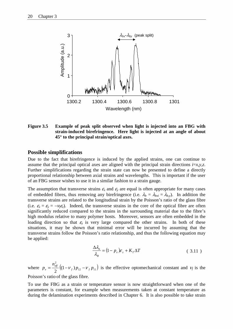
20 Chapter 3
Figure 3.5 Example of peak split observed when light is injected into an FBG with strain-induced birefringence. Here light is injected at an angle of about 45° to the principal strain/optical axes.
Possible simplifications Due to the fact that birefringence is induced by the applied strains, one can continue to assume that the principal optical axes are aligned with the principal strain directions i=x,y,z. Further simplifications regarding the strain state can now be presented to define a directly proportional relationship between axial strains and wavelengths. This is important if the user of an FBG sensor wishes to use it in a similar fashion to a strain gauge.
The assumption that transverse strains εx and εy are equal is often appropriate for many cases of embedded fibres, thus removing any birefringence (i.e. λb = λbxi = λb,y). In addition the transverse strains are related to the longitudinal strain by the Poisson’s ratio of the glass fibre (i.e. εx = εy = −νfεz). Indeed, the transverse strains in the core of the optical fibre are often significantly reduced compared to the strains in the surrounding material due to the fibre’s high modulus relative to many polymer hosts. Moreover, sensors are often embedded in the loading direction so that εz is very large compared the other strains. In both of these situations, it may be shown that minimal error will be incurred by assuming that the transverse strains follow the Poisson’s ratio relationship, and thus the following equation may be applied:
where ( )1112
2
)1(2
ppn
p ffeff
e νν −−= is the effective optomechanical constant and νf is the
Poisson’s ratio of the glass fibre.
To use the FBG as a strain or temperature sensor is now straightforward when one of the parameters is constant, for example when measurements taken at constant temperature as during the delamination experiments described in Chapter 6. It is also possible to take strain
( ) TKp TzeB
b Δ+−=Δ ελλ
1 ( 3.11 )
0
1
2
3
1300.2 1300.4 1300.6 1300.8 1301
Wavelength (nm)
Am
plitu
de (
a.u.
)
λbx-λby (peak split)
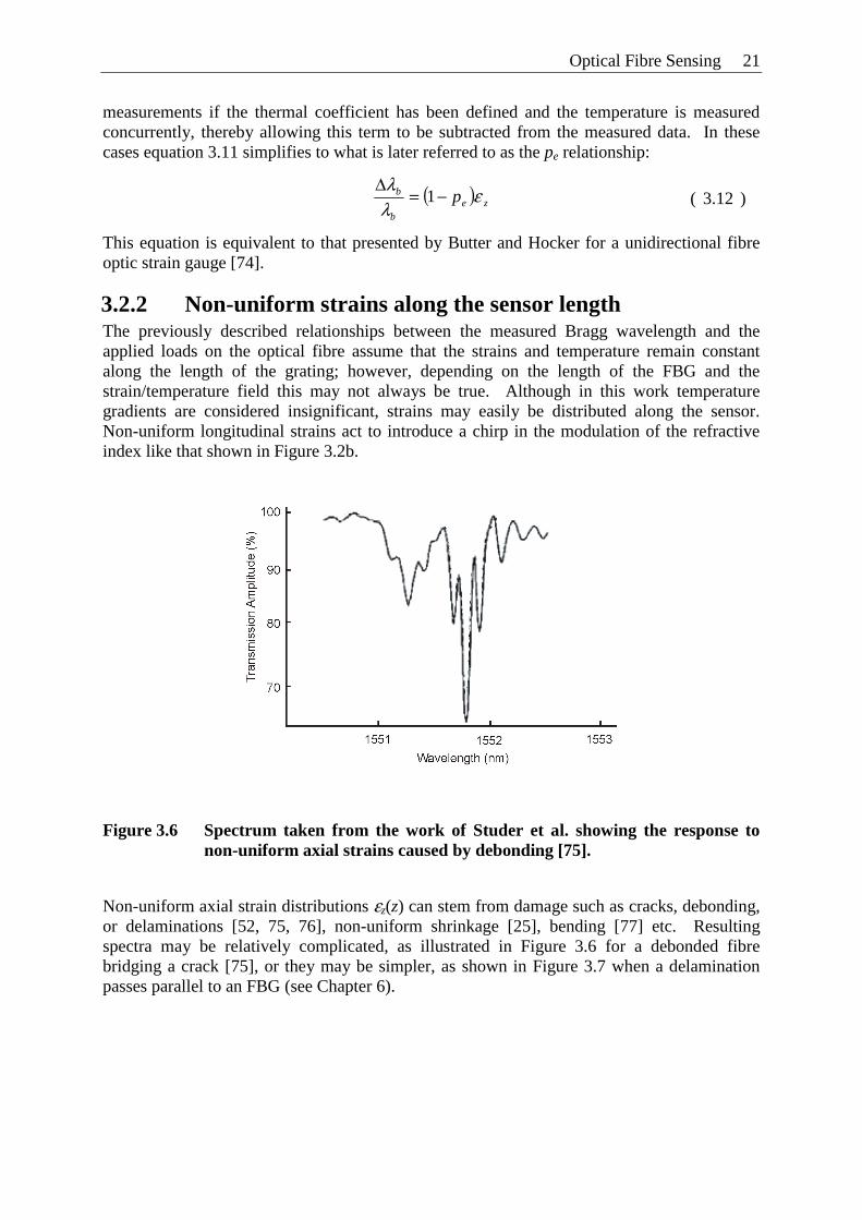
Optical Fibre Sensing 21
measurements if the thermal coefficient has been defined and the temperature is measured concurrently, thereby allowing this term to be subtracted from the measured data. In these cases equation 3.11 simplifies to what is later referred to as the pe relationship:
This equation is equivalent to that presented by Butter and Hocker for a unidirectional fibre optic strain gauge [74].
3.2.2 Non-uniform strains along the sensor length The previously described relationships between the measured Bragg wavelength and the applied loads on the optical fibre assume that the strains and temperature remain constant along the length of the grating; however, depending on the length of the FBG and the strain/temperature field this may not always be true. Although in this work temperature gradients are considered insignificant, strains may easily be distributed along the sensor. Non-uniform longitudinal strains act to introduce a chirp in the modulation of the refractive index like that shown in Figure 3.2b.
Figure 3.6 Spectrum taken from the work of Studer et al. showing the response to non-uniform axial strains caused by debonding [75].
Non-uniform axial strain distributions εz(z) can stem from damage such as cracks, debonding, or delaminations [52, 75, 76], non-uniform shrinkage [25], bending [77] etc. Resulting spectra may be relatively complicated, as illustrated in Figure 3.6 for a debonded fibre bridging a crack [75], or they may be simpler, as shown in Figure 3.7 when a delamination passes parallel to an FBG (see Chapter 6).
( ) zeb
b p ελλ
−=Δ
1 ( 3.12 )
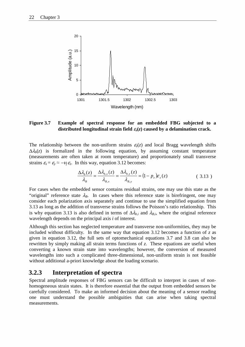
22 Chapter 3
0
5
10
15
20
1301 1301.5 1302 1302.5 1303
Wavelength (nm)
Am
plitu
de (a
.u.)
Figure 3.7 Example of spectral response for an embedded FBG subjected to a distributed longitudinal strain field εz(z) caused by a delamination crack.
The relationship between the non-uniform strains εz(z) and local Bragg wavelength shifts Δλb(z) is formalized in the following equation, by assuming constant temperature (measurements are often taken at room temperature) and proportionately small transverse strains εx = εy ≈ −νf εz. In this way, equation 3.12 becomes:
For cases when the embedded sensor contains residual strains, one may use this state as the “original” reference state λB. In cases where this reference state is birefringent, one may consider each polarization axis separately and continue to use the simplified equation from 3.13 as long as the addition of transverse strains follows the Poisson’s ratio relationship. This is why equation 3.13 is also defined in terms of Δλb,i and λB,i, where the original reference wavelength depends on the principal axis i of interest.
Although this section has neglected temperature and transverse non-uniformities, they may be included without difficulty. In the same way that equation 3.12 becomes a function of z as given in equation 3.12, the full sets of optomechanical equations 3.7 and 3.8 can also be rewritten by simply making all strain terms functions of z. These equations are useful when converting a known strain state into wavelengths; however, the conversion of measured wavelengths into such a complicated three-dimensional, non-uniform strain is not feasible without additional a-priori knowledge about the loading scenario.
3.2.3 Interpretation of spectra Spectral amplitude responses of FBG sensors can be difficult to interpret in cases of non-homogeneous strain states. It is therefore essential that the output from embedded sensors be carefully considered. To make an informed decision about the meaning of a sensor reading one must understand the possible ambiguities that can arise when taking spectral measurements.
( ) )(1)()()(
,
,
,
, zpzzz
zeyB
yb
xB
xb
B
b ελλ
λλ
λλ
−=Δ
=Δ
=Δ
( 3.13 )
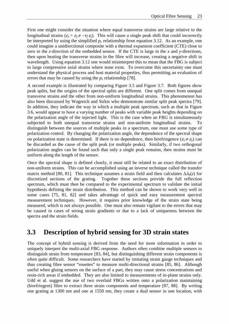
Optical Fibre Sensing 23
First one might consider the situation where equal transverse strains are large relative to the longitudinal strains (εx = εy ≠ −νf εz). This will cause a single peak shift that could incorrectly be interpreted by using the simplified pe relationship from equation 3.12. As an example, one could imagine a unidirectional composite with a thermal expansion coefficient (CTE) close to zero in the z-direction of the embedded sensor. If the CTE is large in the x and y-directions, then upon heating the transverse strains in the fibre will increase, creating a negative shift in wavelength. Using equation 3.12 one would misinterpret this to mean that the FBG is subject to large compressive axial strains where none exist. To overcome this uncertainty one must understand the physical process and host material properties, thus permitting an evaluation of errors that may be caused by using the pe relationship [78].
A second example is illustrated by comparing Figure 3.5 and Figure 3.7. Both figures show peak splits, but the origins of the spectral splits are different. One split comes from unequal transverse strains and the other from non-uniform longitudinal strains. This phenomenon has also been discussed by Wagreich and Sirkis who demonstrate similar split peak spectra [79]. In addition, they indicate the way in which a multiple peak spectrum, such as that in Figure 3.6, would appear to have a varying number of peaks with variable peak heights depending on the polarization angle of the injected light. This is the case when an FBG is simultaneously subjected to both unequal transverse strains and non-uniform longitudinal strains. To distinguish between the sources of multiple peaks in a spectrum, one must use some type of polarization control. By changing the polarization angle, the dependence of the spectral shape on polarization state is determined. If there is no dependence, then birefringence (εx ≠ εy) can be discarded as the cause of the split peak (or multiple peaks). Similarly, if two orthogonal polarization angles can be found such that only a single peak remains, then strains must be uniform along the length of the sensor.
Once the spectral shape is defined clearly, it must still be related to an exact distribution of non-uniform strains. This can be accomplished using an inverse technique called the transfer matrix method [80, 81]. This technique assumes a strain field and then calculates Δλb(z) for discretized sections of the grating. Together these sections provide the full reflection spectrum, which must then be compared to the experimental spectrum to validate the initial hypothesis defining the strain distribution. This method can be shown to work very well in some cases [75, 81, 82] and takes advantage of quick and easy measurement spectral measurement techniques. However, it requires prior knowledge of the strain state being measured, which is not always possible. One must also remain vigilant to the errors that may be caused in cases of strong strain gradients or due to a lack of uniqueness between the spectra and the strain fields.
3.3 Description of hybrid sensing for 3D strain states
The concept of hybrid sensing is derived from the need for more information in order to uniquely interpret the multi-axial FBG response. Authors often combine multiple sensors to distinguish strain from temperature [83, 84], but distinguishing different strain components is often quite difficult. Some researchers have started by imitating strain gauge techniques and thus creating fibre sensor “rosettes” to measure multi-directional strains [85, 86]. Although useful when gluing sensors on the surface of a part, they may cause stress concentrations and resin-rich areas if embedded. They are also limited to measurements of in-plane strains only. Udd et al. suggest the use of two overlaid FBGs written onto a polarization maintaining (birefringent) fibre to extract three strain components and temperature [87, 88]. By writing one grating at 1300 nm and one at 1550 nm, they create a dual sensor in one location, with
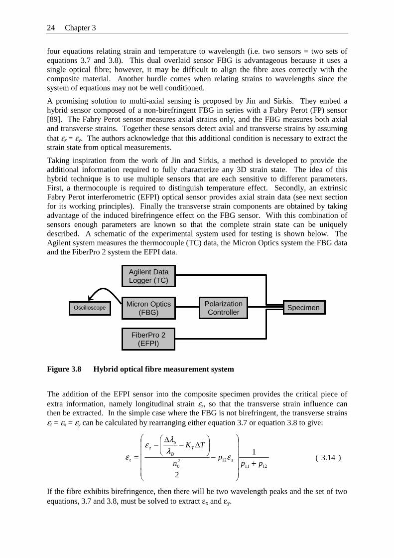
24 Chapter 3
four equations relating strain and temperature to wavelength (i.e. two sensors = two sets of equations 3.7 and 3.8). This dual overlaid sensor FBG is advantageous because it uses a single optical fibre; however, it may be difficult to align the fibre axes correctly with the composite material. Another hurdle comes when relating strains to wavelengths since the system of equations may not be well conditioned.
A promising solution to multi-axial sensing is proposed by Jin and Sirkis. They embed a hybrid sensor composed of a non-birefringent FBG in series with a Fabry Perot (FP) sensor [89]. The Fabry Perot sensor measures axial strains only, and the FBG measures both axial and transverse strains. Together these sensors detect axial and transverse strains by assuming that εx = εy. The authors acknowledge that this additional condition is necessary to extract the strain state from optical measurements.
Taking inspiration from the work of Jin and Sirkis, a method is developed to provide the additional information required to fully characterize any 3D strain state. The idea of this hybrid technique is to use multiple sensors that are each sensitive to different parameters. First, a thermocouple is required to distinguish temperature effect. Secondly, an extrinsic Fabry Perot interferometric (EFPI) optical sensor provides axial strain data (see next section for its working principles). Finally the transverse strain components are obtained by taking advantage of the induced birefringence effect on the FBG sensor. With this combination of sensors enough parameters are known so that the complete strain state can be uniquely described. A schematic of the experimental system used for testing is shown below. The Agilent system measures the thermocouple (TC) data, the Micron Optics system the FBG data and the FiberPro 2 system the EFPI data.
Figure 3.8 Hybrid optical fibre measurement system
The addition of the EFPI sensor into the composite specimen provides the critical piece of extra information, namely longitudinal strain εz, so that the transverse strain influence can then be extracted. In the simple case where the FBG is not birefringent, the transverse strains εt = εx = εy can be calculated by rearranging either equation 3.7 or equation 3.8 to give:
If the fibre exhibits birefringence, then there will be two wavelength peaks and the set of two equations, 3.7 and 3.8, must be solved to extract εx and εy.
1211
1220
1
2
ppp
n
TK
z
TB
bz
t +⎟⎟⎟⎟⎟
⎠
⎞
⎜⎜⎜⎜⎜
⎝
⎛
−⎟⎟⎠
⎞⎜⎜⎝
⎛Δ−
Δ−
= ελλε
ε ( 3.14 )
Micron Optics (FBG)
FiberPro 2 (EFPI)
Polarization Controller
Oscilloscope
Agilent Data Logger (TC)
Specimen
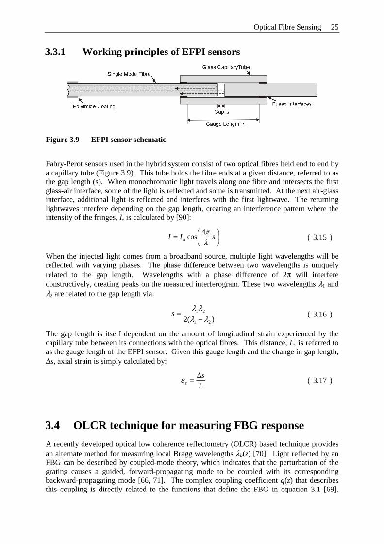
Optical Fibre Sensing 25
3.3.1 Working principles of EFPI sensors
Figure 3.9 EFPI sensor schematic
Fabry-Perot sensors used in the hybrid system consist of two optical fibres held end to end by a capillary tube (Figure 3.9). This tube holds the fibre ends at a given distance, referred to as the gap length (s). When monochromatic light travels along one fibre and intersects the first glass-air interface, some of the light is reflected and some is transmitted. At the next air-glass interface, additional light is reflected and interferes with the first lightwave. The returning lightwaves interfere depending on the gap length, creating an interference pattern where the intensity of the fringes, I, is calculated by [90]:
When the injected light comes from a broadband source, multiple light wavelengths will be reflected with varying phases. The phase difference between two wavelengths is uniquely related to the gap length. Wavelengths with a phase difference of 2π will interfere constructively, creating peaks on the measured interferogram. These two wavelengths λ1 and λ2 are related to the gap length via:
The gap length is itself dependent on the amount of longitudinal strain experienced by the capillary tube between its connections with the optical fibres. This distance, L, is referred to as the gauge length of the EFPI sensor. Given this gauge length and the change in gap length, Δs, axial strain is simply calculated by:
3.4 OLCR technique for measuring FBG response
A recently developed optical low coherence reflectometry (OLCR) based technique provides an alternate method for measuring local Bragg wavelengths λb(z) [70]. Light reflected by an FBG can be described by coupled-mode theory, which indicates that the perturbation of the grating causes a guided, forward-propagating mode to be coupled with its corresponding backward-propagating mode [66, 71]. The complex coupling coefficient q(z) that describes this coupling is directly related to the functions that define the FBG in equation 3.1 [69].
⎟⎠⎞
⎜⎝⎛= sII o λ
π4cos
( 3.15 )
)(2 21
21
λλλλ−
=s
( 3.16 )
L
sz
Δ=ε
( 3.17 )
26 Chapter 3
Consequently, the phase φ(z) of q(z) can be related to the local wavelength, thereby removing any need to make assumptions about the form of εz(z). The following sections explain this technique and the relationship between phase and wavelength. They also describe modifications to the system which allow measurements in non-homogeneous strain fields where birefringence is induced in the sensor due to εx ≠ εy.
3.4.1 Description of OLCR-based system The OLCR system used for measuring non-uniform strain fields consists of a test arm and a reference arm that forms a Michelson type interferometer. As illustrated in Figure 3.10, light from a low-coherence source (LED) is split and sent along the two arms, reflected by both the FBG in the test arm and a moveable mirror in the reference arm, and finally interfering at the coupler. Due to the small coherence length of the source, only light that has travelled the same distance (within ±10μm coherence length of the LED source) will interfere, thus rendering the resulting information position (z-direction) dependent.
LED
Data Acquisition
Translating Stage
Mirror
)()( ziezq
φ
Test Arm Reference Arm
Time-domain Spatial-domain
FBG
Coupler
LED
Data Acquisition
Translating Stage
Mirror
)()( ziezq
φ
Test Arm Reference Arm
Time-domain Spatial-domain
FBG
Coupler
Figure 3.10 Simplified schematic of OLCR-based measurement system constructed by P. Giaccari. A more detailed schematic can be found in [70].
By moving the reference arm mirror, it is possible to detect the light reflected from varying locations within the low-birefringent FBG sensor. The convolution of the source and the complex impulse response h(t) (t represents time) of the light is collected for discrete locations within the sensor. Discrete values of h(t) are then inserted into an inverse scattering algorithm that calculates amplitude |q(z)| and phase φ (z) of the coupling coefficient q(z) as a function of position inside the grating [69]. The local Bragg wavelength λb(z) in a non-birefringent fibre can be calculated as:
where λd is a reference wavelength chosen within the range reflected by the FBG. Typical measurements of a free (unembedded) 22mm long FBG are shown in Figure 3.11. Here one sees plots of the impulse amplitude and spectral amplitude along with the corresponding distribution of λb(z). It is clear here that the fibre is homogeneous and unchirped. Figure 3.12 provides a typical phase measurement φ (z) that is used in equation 3.18 to calculate λb(z).
( ) ( )1
4
11−
⎪⎭
⎪⎬⎫
⎪⎩
⎪⎨⎧
⋅+=dz
zd
nz
effdb
φπλ
λ ( 3.18 )
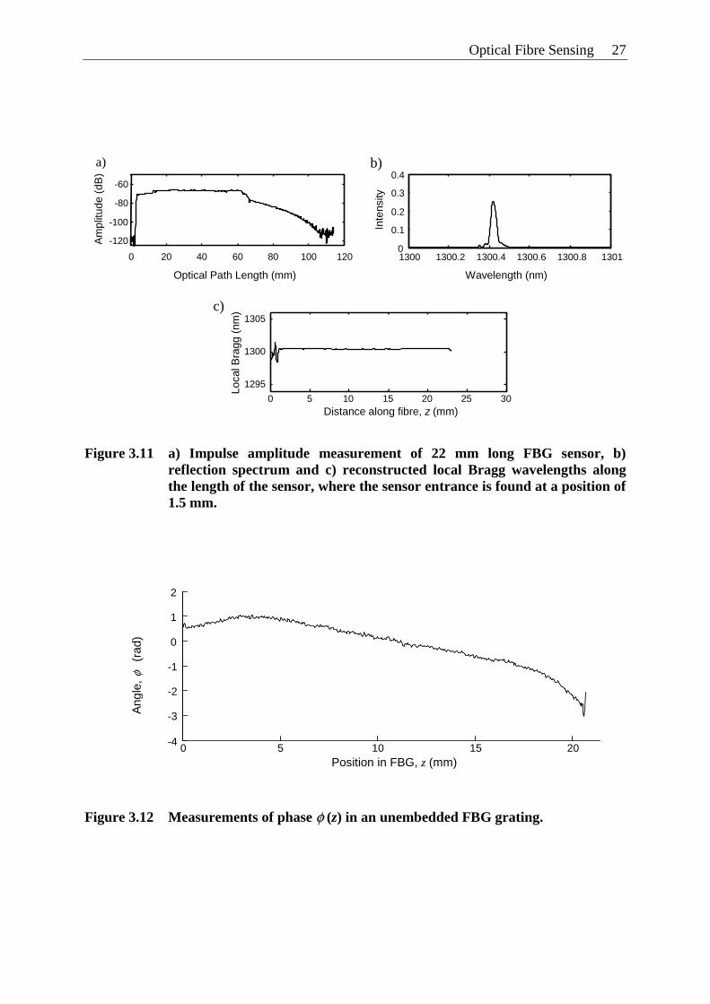
Optical Fibre Sensing 27
Figure 3.11 a) Impulse amplitude measurement of 22 mm long FBG sensor, b) reflection spectrum and c) reconstructed local Bragg wavelengths along the length of the sensor, where the sensor entrance is found at a position of 1.5 mm.
Figure 3.12 Measurements of phase φ (z) in an unembedded FBG grating.
0 5 10 15 20 -4
-3
-2
-1
0
1
2
Ang
le, φ
(r
ad)
Position in FBG, z (mm)
0 5 10 15 20 25 30
1295
1300
1305
Loca
l Bra
gg (
nm)
Distance along fibre, z (mm)
0 20 40 60 80 100 120
-120
-100
-80
-60
Am
plitu
de (
dB)
1300 1300.2 1300.4 1300.6 1300.8 1301 0
0.1
0.2
0.3
0.4
Inte
nsity
Optical Path Length (mm) Wavelength (nm)
c)
b) a)
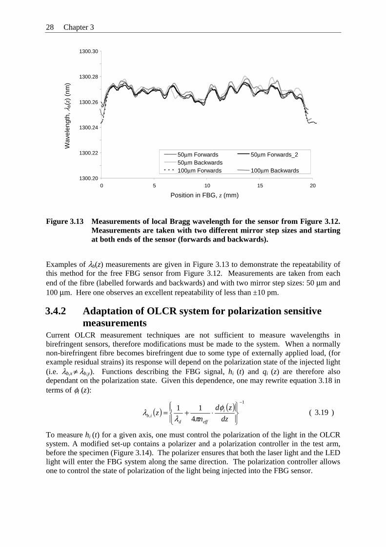
28 Chapter 3
Figure 3.13 Measurements of local Bragg wavelength for the sensor from Figure 3.12. Measurements are taken with two different mirror step sizes and starting at both ends of the sensor (forwards and backwards).
Examples of λb(z) measurements are given in Figure 3.13 to demonstrate the repeatability of this method for the free FBG sensor from Figure 3.12. Measurements are taken from each end of the fibre (labelled forwards and backwards) and with two mirror step sizes: 50 μm and 100 μm. Here one observes an excellent repeatability of less than ±10 pm.
3.4.2 Adaptation of OLCR system for polarization sensitive measurements
Current OLCR measurement techniques are not sufficient to measure wavelengths in birefringent sensors, therefore modifications must be made to the system. When a normally non-birefringent fibre becomes birefringent due to some type of externally applied load, (for example residual strains) its response will depend on the polarization state of the injected light (i.e. λb,x ≠ λb,y). Functions describing the FBG signal, hi (t) and qi (z) are therefore also dependant on the polarization state. Given this dependence, one may rewrite equation 3.18 in terms of φi (z):
To measure hi (t) for a given axis, one must control the polarization of the light in the OLCR system. A modified set-up contains a polarizer and a polarization controller in the test arm, before the specimen (Figure 3.14). The polarizer ensures that both the laser light and the LED light will enter the FBG system along the same direction. The polarization controller allows one to control the state of polarization of the light being injected into the FBG sensor.
( ) ( ) 1
, 4
11−
⎪⎭
⎪⎬⎫
⎪⎩
⎪⎨⎧
⋅+=dz
zd
nz i
effdib
φπλ
λ ( 3.19 )
1300.20
1300.22
1300.24
1300.26
1300.28
1300.30
0 5 10 15 20 Position in FBG, z (mm)
50μm Forwards 50μm Forwards_2 50μm Backwards
100μm Backwards100μm Forwards
Wav
elen
gth,
λb(
z) (
nm)
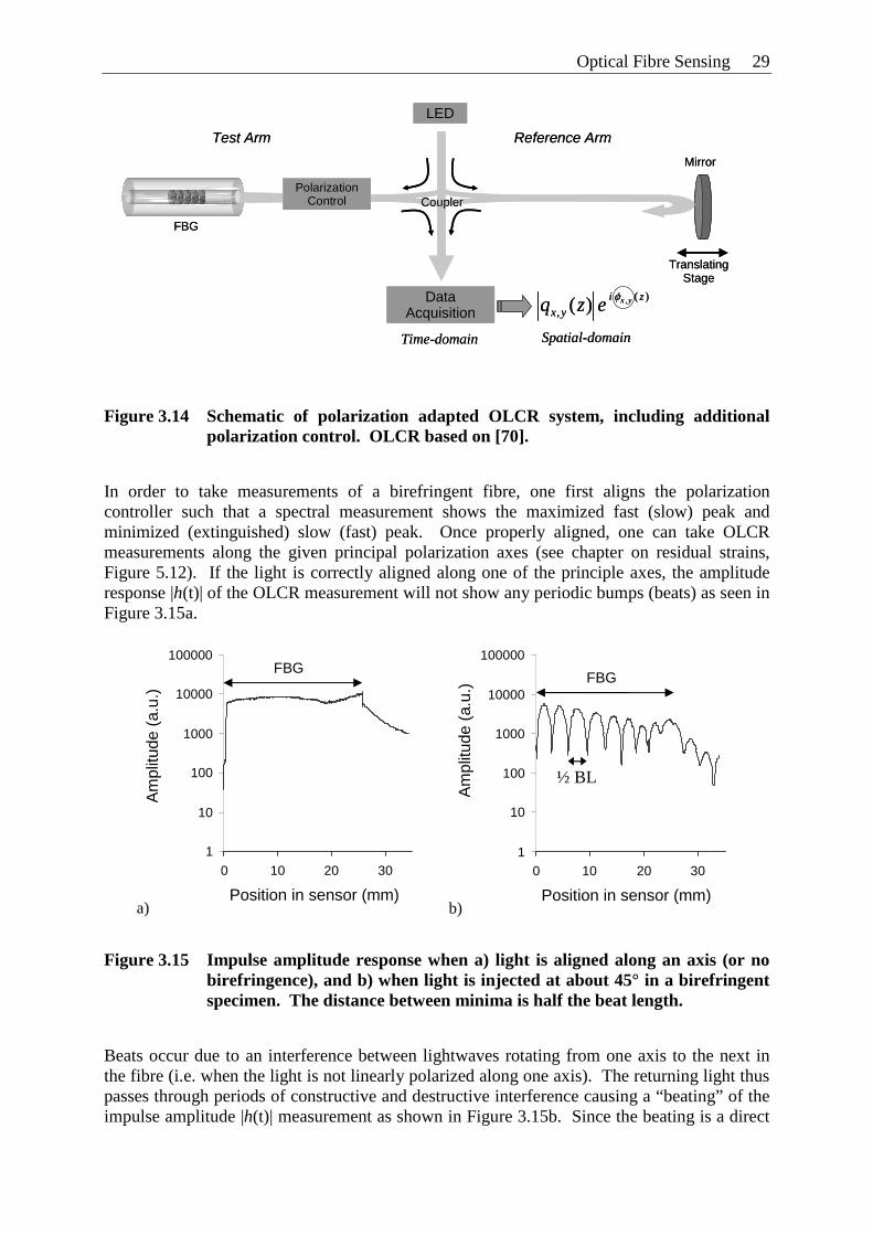
Optical Fibre Sensing 29
LED
Data Acquisition
Polarization Control
Translating Stage
Mirror
)(,
,)( zi
yxyxezq
φ
Test Arm Reference Arm
Time-domain Spatial-domain
FBG
Coupler
LED
Data Acquisition
Polarization Control
Translating Stage
Mirror
)(,
,)( zi
yxyxezq
φ
Test Arm Reference Arm
Time-domain Spatial-domain
FBG
Coupler
Figure 3.14 Schematic of polarization adapted OLCR system, including additional polarization control. OLCR based on [70].
In order to take measurements of a birefringent fibre, one first aligns the polarization controller such that a spectral measurement shows the maximized fast (slow) peak and minimized (extinguished) slow (fast) peak. Once properly aligned, one can take OLCR measurements along the given principal polarization axes (see chapter on residual strains, Figure 5.12). If the light is correctly aligned along one of the principle axes, the amplitude response |h(t)| of the OLCR measurement will not show any periodic bumps (beats) as seen in Figure 3.15a.
Figure 3.15 Impulse amplitude response when a) light is aligned along an axis (or no birefringence), and b) when light is injected at about 45° in a birefringent specimen. The distance between minima is half the beat length.
Beats occur due to an interference between lightwaves rotating from one axis to the next in the fibre (i.e. when the light is not linearly polarized along one axis). The returning light thus passes through periods of constructive and destructive interference causing a “beating” of the impulse amplitude |h(t)| measurement as shown in Figure 3.15b. Since the beating is a direct
1
10
100
1000
10000
100000
0 10 20 30
Position in sensor (mm)
Am
plitu
de (
a.u.
)
½ BL
FBG
b)
1
10
100
1000
10000
100000
0 10 20 30
Position in sensor (mm)
Am
plitu
de (
a.u.
)
FBG
a)

30 Chapter 3
consequence of the birefringence, the spatial path length between minima (i.e. beat length=BL) can be related to the difference between the effective refractive indices of each axis [91]:
This can be used as an independent verification of the quality of the alignment or the degree of birefringence.
BL
nn Byeffxeff
λ=− ,, ( 3.20 )

Chapter 4 Materials and Methods
The studies carried out in this thesis work are based on the integration of optical fibre sensors in composite laminates. Most of these investigations use carbon fibre-reinforced polyphenylene sulphide laminated composites and fibre Bragg grating sensors; therefore, this chapter is dedicated to providing a more complete understanding of this composite system and its corresponding production procedure. It is also important to define the sensitivities of the FBG sensors and to explain how these sensors are integrated into the composite plates. This chapter finishes by summarizing the various composite plate–optical sensor configurations fabricated for testing.
4.1 Composite plate preparation
Composite laminates are produced from Cytec’s AS4/PPS (carbon fibre – polyphenylene sulphide) Fiberite composite prepreg. The advantages of this semi-crystalline thermoplastic composite are its excellent high temperature and chemical resistance. The disadvantage of the matrix system is its low fracture toughness, which can lead to microcracking during processing [12].
Figure 4.1 a) Pre-preg plies stacked in steel mould. b) Mould in hot-press (plastic release film prevents sticking to top platen).
a) b)
Mould frame Exit slot
Composite pre-preg
Hydraulic Press
Mould
Release film
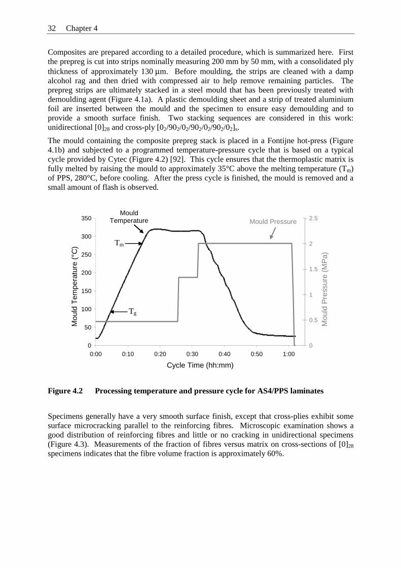
32 Chapter 4
Composites are prepared according to a detailed procedure, which is summarized here. First the prepreg is cut into strips nominally measuring 200 mm by 50 mm, with a consolidated ply thickness of approximately 130 μm. Before moulding, the strips are cleaned with a damp alcohol rag and then dried with compressed air to help remove remaining particles. The prepreg strips are ultimately stacked in a steel mould that has been previously treated with demoulding agent (Figure 4.1a). A plastic demoulding sheet and a strip of treated aluminium foil are inserted between the mould and the specimen to ensure easy demoulding and to provide a smooth surface finish. Two stacking sequences are considered in this work: unidirectional [0]28 and cross-ply [02/902/02/902/02/902/02]s.
The mould containing the composite prepreg stack is placed in a Fontijne hot-press (Figure 4.1b) and subjected to a programmed temperature-pressure cycle that is based on a typical cycle provided by Cytec (Figure 4.2) [92]. This cycle ensures that the thermoplastic matrix is fully melted by raising the mould to approximately 35°C above the melting temperature (Tm) of PPS, 280°C, before cooling. After the press cycle is finished, the mould is removed and a small amount of flash is observed.
Figure 4.2 Processing temperature and pressure cycle for AS4/PPS laminates
Specimens generally have a very smooth surface finish, except that cross-plies exhibit some surface microcracking parallel to the reinforcing fibres. Microscopic examination shows a good distribution of reinforcing fibres and little or no cracking in unidirectional specimens (Figure 4.3). Measurements of the fraction of fibres versus matrix on cross-sections of [0]28 specimens indicates that the fibre volume fraction is approximately 60%.
0
50
100
150
200
250
300
350
0:00 0:10 0:20 0:30 0:40 0:50 1:00
Cycle Time (hh:mm)
Mou
ld T
empe
ratu
re (
°C)
0
0.5
1
1.5
2
2.5
Mou
ld P
ress
ure
(MP
a)
Mould Pressure Mould
Temperature
Tm
Tg
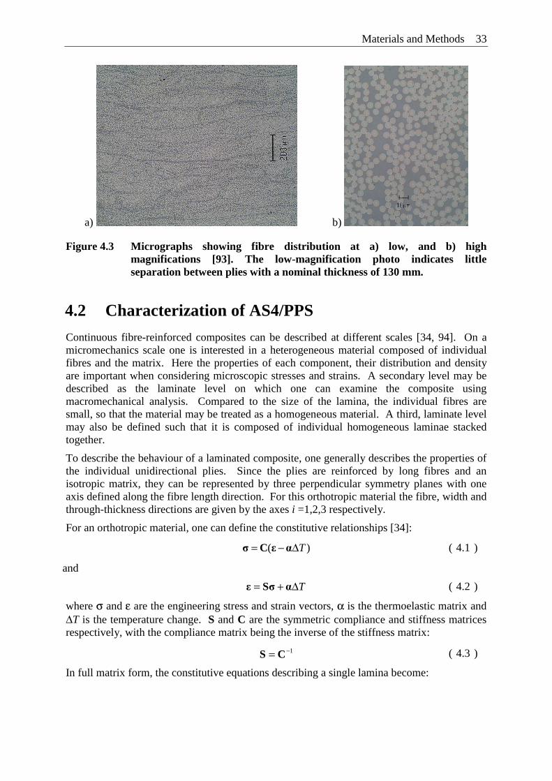
Materials and Methods 33
a)
b)
Figure 4.3 Micrographs showing fibre distribution at a) low, and b) high magnifications [93]. The low-magnification photo indicates little separation between plies with a nominal thickness of 130 mm.
4.2 Characterization of AS4/PPS
Continuous fibre-reinforced composites can be described at different scales [34, 94]. On a micromechanics scale one is interested in a heterogeneous material composed of individual fibres and the matrix. Here the properties of each component, their distribution and density are important when considering microscopic stresses and strains. A secondary level may be described as the laminate level on which one can examine the composite using macromechanical analysis. Compared to the size of the lamina, the individual fibres are small, so that the material may be treated as a homogeneous material. A third, laminate level may also be defined such that it is composed of individual homogeneous laminae stacked together.
To describe the behaviour of a laminated composite, one generally describes the properties of the individual unidirectional plies. Since the plies are reinforced by long fibres and an isotropic matrix, they can be represented by three perpendicular symmetry planes with one axis defined along the fibre length direction. For this orthotropic material the fibre, width and through-thickness directions are given by the axes i =1,2,3 respectively.
For an orthotropic material, one can define the constitutive relationships [34]:
where σ and ε are the engineering stress and strain vectors, α is the thermoelastic matrix and ΔT is the temperature change. S and C are the symmetric compliance and stiffness matrices respectively, with the compliance matrix being the inverse of the stiffness matrix:
In full matrix form, the constitutive equations describing a single lamina become:
)( TΔ−= αεCσ ( 4.1 )
and
TΔ+= αSσε ( 4.2 )
1−= CS ( 4.3 )
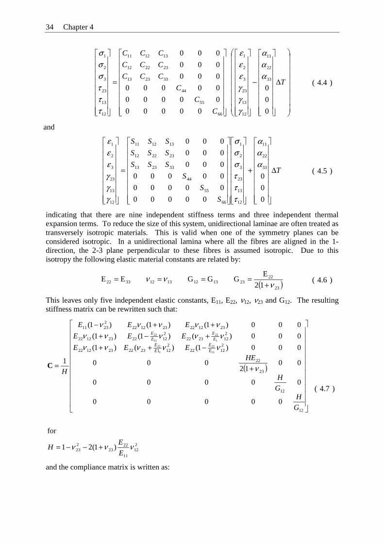
34 Chapter 4
indicating that there are nine independent stiffness terms and three independent thermal expansion terms. To reduce the size of this system, unidirectional laminae are often treated as transversely isotropic materials. This is valid when one of the symmetry planes can be considered isotropic. In a unidirectional lamina where all the fibres are aligned in the 1-direction, the 2-3 plane perpendicular to these fibres is assumed isotropic. Due to this isotropy the following elastic material constants are related by:
This leaves only five independent elastic constants, E11, E22, ν12, ν23 and G12. The resulting stiffness matrix can be rewritten such that:
and the compliance matrix is written as:
⎟⎟⎟⎟⎟⎟⎟⎟
⎠
⎞
⎜⎜⎜⎜⎜⎜⎜⎜
⎝
⎛
Δ
⎥⎥⎥⎥⎥⎥⎥⎥
⎦
⎤
⎢⎢⎢⎢⎢⎢⎢⎢
⎣
⎡
−
⎥⎥⎥⎥⎥⎥⎥⎥
⎦
⎤
⎢⎢⎢⎢⎢⎢⎢⎢
⎣
⎡
⎥⎥⎥⎥⎥⎥⎥⎥
⎦
⎤
⎢⎢⎢⎢⎢⎢⎢⎢
⎣
⎡
=
⎥⎥⎥⎥⎥⎥⎥⎥
⎦
⎤
⎢⎢⎢⎢⎢⎢⎢⎢
⎣
⎡
T
C
C
C
CCC
CCC
CCC
0
0
0
00000
00000
00000
000
000
000
33
22
11
12
13
23
3
2
1
66
55
44
332313
232212
131211
12
13
23
3
2
1
ααα
γγγεεε
τττσσσ
( 4.4 )
and
T
S
S
S
SSS
SSS
SSS
Δ
⎥⎥⎥⎥⎥⎥⎥⎥
⎦
⎤
⎢⎢⎢⎢⎢⎢⎢⎢
⎣
⎡
+
⎥⎥⎥⎥⎥⎥⎥⎥
⎦
⎤
⎢⎢⎢⎢⎢⎢⎢⎢
⎣
⎡
⎥⎥⎥⎥⎥⎥⎥⎥
⎦
⎤
⎢⎢⎢⎢⎢⎢⎢⎢
⎣
⎡
=
⎥⎥⎥⎥⎥⎥⎥⎥
⎦
⎤
⎢⎢⎢⎢⎢⎢⎢⎢
⎣
⎡
0
0
0
00000
00000
00000
000
000
000
33
22
11
12
13
23
3
2
1
66
55
44
332313
232212
131211
12
13
23
3
2
1
ααα
τττσσσ
γγγεεε
( 4.5 )
( )23
2223131213123322 12
EGGGEE
ννν
+==== ( 4.6 )
( )
212
11
2223
223
12
12
23
22
21222
21212322231222
2122322
21222231222
23122223122222311
)1(21
for
00000
00000
0012
000
000)1()()1(
000)()1()1(
000)1()1()1(
111
22
1
22
1
22
11
22
ννν
ν
νννννννννν
ννννν
E
EH
G
HG
H
HEEEE
EEE
EEE
H
EE
EE
EE
EE
+−−=
⎥⎥⎥⎥⎥⎥⎥⎥⎥⎥⎥
⎦
⎤
⎢⎢⎢⎢⎢⎢⎢⎢⎢⎢⎢
⎣
⎡
+
−+++−+
++−
=C
( 4.7 )
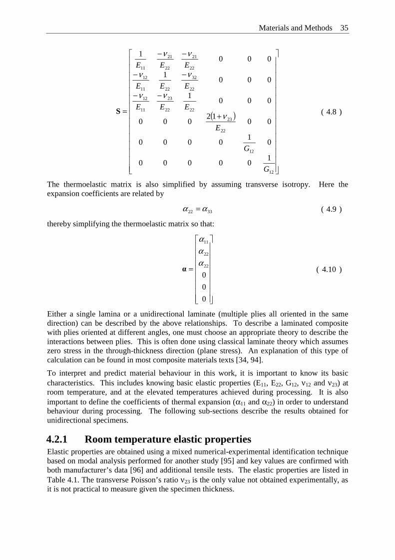
Materials and Methods 35
The thermoelastic matrix is also simplified by assuming transverse isotropy. Here the expansion coefficients are related by
thereby simplifying the thermoelastic matrix so that:
Either a single lamina or a unidirectional laminate (multiple plies all oriented in the same direction) can be described by the above relationships. To describe a laminated composite with plies oriented at different angles, one must choose an appropriate theory to describe the interactions between plies. This is often done using classical laminate theory which assumes zero stress in the through-thickness direction (plane stress). An explanation of this type of calculation can be found in most composite materials texts [34, 94].
To interpret and predict material behaviour in this work, it is important to know its basic characteristics. This includes knowing basic elastic properties (E11, E22, G12, ν12 and ν23) at room temperature, and at the elevated temperatures achieved during processing. It is also important to define the coefficients of thermal expansion (α11 and α22) in order to understand behaviour during processing. The following sub-sections describe the results obtained for unidirectional specimens.
4.2.1 Room temperature elastic properties Elastic properties are obtained using a mixed numerical-experimental identification technique based on modal analysis performed for another study [95] and key values are confirmed with both manufacturer’s data [96] and additional tensile tests. The elastic properties are listed in Table 4.1. The transverse Poisson’s ratio ν23 is the only value not obtained experimentally, as it is not practical to measure given the specimen thickness.
( )
⎥⎥⎥⎥⎥⎥⎥⎥⎥⎥⎥⎥⎥⎥⎥
⎦
⎤
⎢⎢⎢⎢⎢⎢⎢⎢⎢⎢⎢⎢⎢⎢⎢
⎣
⎡
+
−−
−−
−−
=
12
12
22
23
2222
23
11
12
22
32
2211
12
22
21
22
21
11
100000
01
0000
0012
000
0001
0001
0001
G
G
E
EEE
EEE
EEE
ν
νν
νν
νν
S ( 4.8 )
3322 αα = ( 4.9 )
⎥⎥⎥⎥⎥⎥⎥⎥
⎦
⎤
⎢⎢⎢⎢⎢⎢⎢⎢
⎣
⎡
=
0
0
022
22
11
ααα
α ( 4.10 )
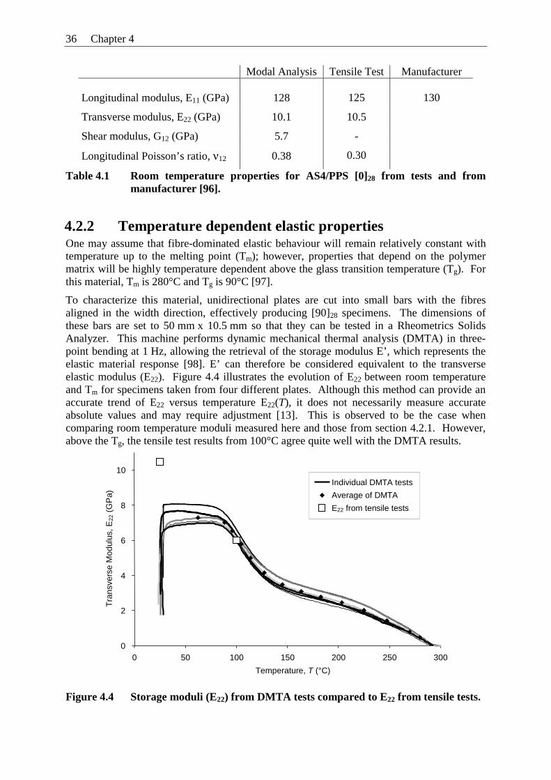
36 Chapter 4
Modal Analysis Tensile Test Manufacturer Longitudinal modulus, E11 (GPa)
128
125
130
Transverse modulus, E22 (GPa) 10.1 10.5
Shear modulus, G12 (GPa) 5.7 -
Longitudinal Poisson’s ratio, ν12 0.38 0.30
Table 4.1 Room temperature properties for AS4/PPS [0]28 from tests and from manufacturer [96].
4.2.2 Temperature dependent elastic properties One may assume that fibre-dominated elastic behaviour will remain relatively constant with temperature up to the melting point (Tm); however, properties that depend on the polymer matrix will be highly temperature dependent above the glass transition temperature (Tg). For this material, Tm is 280°C and Tg is 90°C [97].
To characterize this material, unidirectional plates are cut into small bars with the fibres aligned in the width direction, effectively producing [90]28 specimens. The dimensions of these bars are set to 50 mm x 10.5 mm so that they can be tested in a Rheometrics Solids Analyzer. This machine performs dynamic mechanical thermal analysis (DMTA) in three-point bending at 1 Hz, allowing the retrieval of the storage modulus E’, which represents the elastic material response [98]. E’ can therefore be considered equivalent to the transverse elastic modulus (E22). Figure 4.4 illustrates the evolution of E22 between room temperature and Tm for specimens taken from four different plates. Although this method can provide an accurate trend of E22 versus temperature E22(T), it does not necessarily measure accurate absolute values and may require adjustment [13]. This is observed to be the case when comparing room temperature moduli measured here and those from section 4.2.1. However, above the Tg, the tensile test results from 100°C agree quite well with the DMTA results.
Figure 4.4 Storage moduli (E22) from DMTA tests compared to E22 from tensile tests.
0
2
4
6
8
10
0 50 100 150 200 250 300
Temperature, T (°C)
Tra
nsve
rse
Mod
ulus
, E22
(G
Pa)
Individual DMTA tests
Average of DMTA E22 from tensile tests
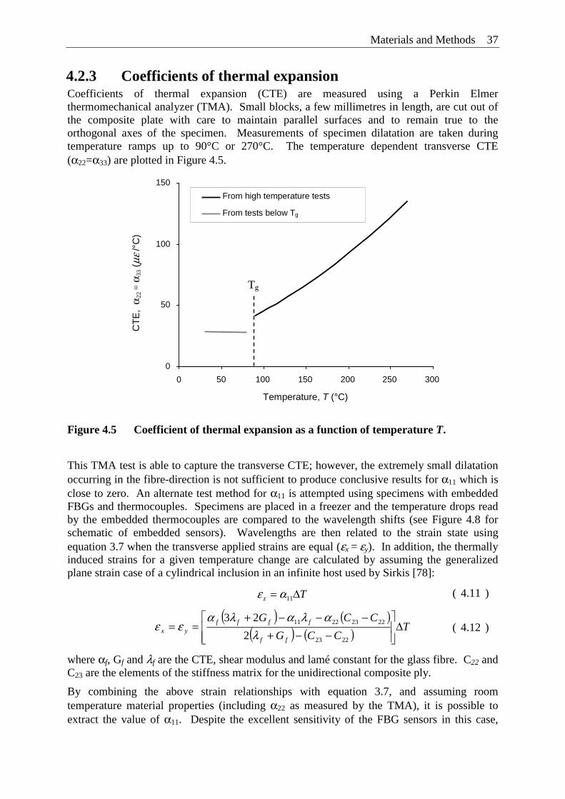
Materials and Methods 37
4.2.3 Coefficients of thermal expansion Coefficients of thermal expansion (CTE) are measured using a Perkin Elmer thermomechanical analyzer (TMA). Small blocks, a few millimetres in length, are cut out of the composite plate with care to maintain parallel surfaces and to remain true to the orthogonal axes of the specimen. Measurements of specimen dilatation are taken during temperature ramps up to 90°C or 270°C. The temperature dependent transverse CTE (α22=α33) are plotted in Figure 4.5.
Figure 4.5 Coefficient of thermal expansion as a function of temperature T.
This TMA test is able to capture the transverse CTE; however, the extremely small dilatation occurring in the fibre-direction is not sufficient to produce conclusive results for α11 which is close to zero. An alternate test method for α11 is attempted using specimens with embedded FBGs and thermocouples. Specimens are placed in a freezer and the temperature drops read by the embedded thermocouples are compared to the wavelength shifts (see Figure 4.8 for schematic of embedded sensors). Wavelengths are then related to the strain state using equation 3.7 when the transverse applied strains are equal (εx = εy). In addition, the thermally induced strains for a given temperature change are calculated by assuming the generalized plane strain case of a cylindrical inclusion in an infinite host used by Sirkis [78]:
where αf, Gf and λf are the CTE, shear modulus and lamé constant for the glass fibre. C22 and C23 are the elements of the stiffness matrix for the unidirectional composite ply.
By combining the above strain relationships with equation 3.7, and assuming room temperature material properties (including α22 as measured by the TMA), it is possible to extract the value of α11. Despite the excellent sensitivity of the FBG sensors in this case,
Tz Δ= 11αε ( 4.11 )
( ) ( )
( ) ( ) TCCG
CCG
ff
ffffyx Δ
⎥⎥⎦
⎤
⎢⎢⎣
⎡
−−+−−−+
==2223
22232211
2
23
λαλαλα
εε ( 4.12 )
0
50
100
150
0 50 100 150 200 250 300
Temperature, T (°C)
From high temperature tests
From tests below Tg
CT
E,
α 22 =
α33
(με
/°C
)
Tg
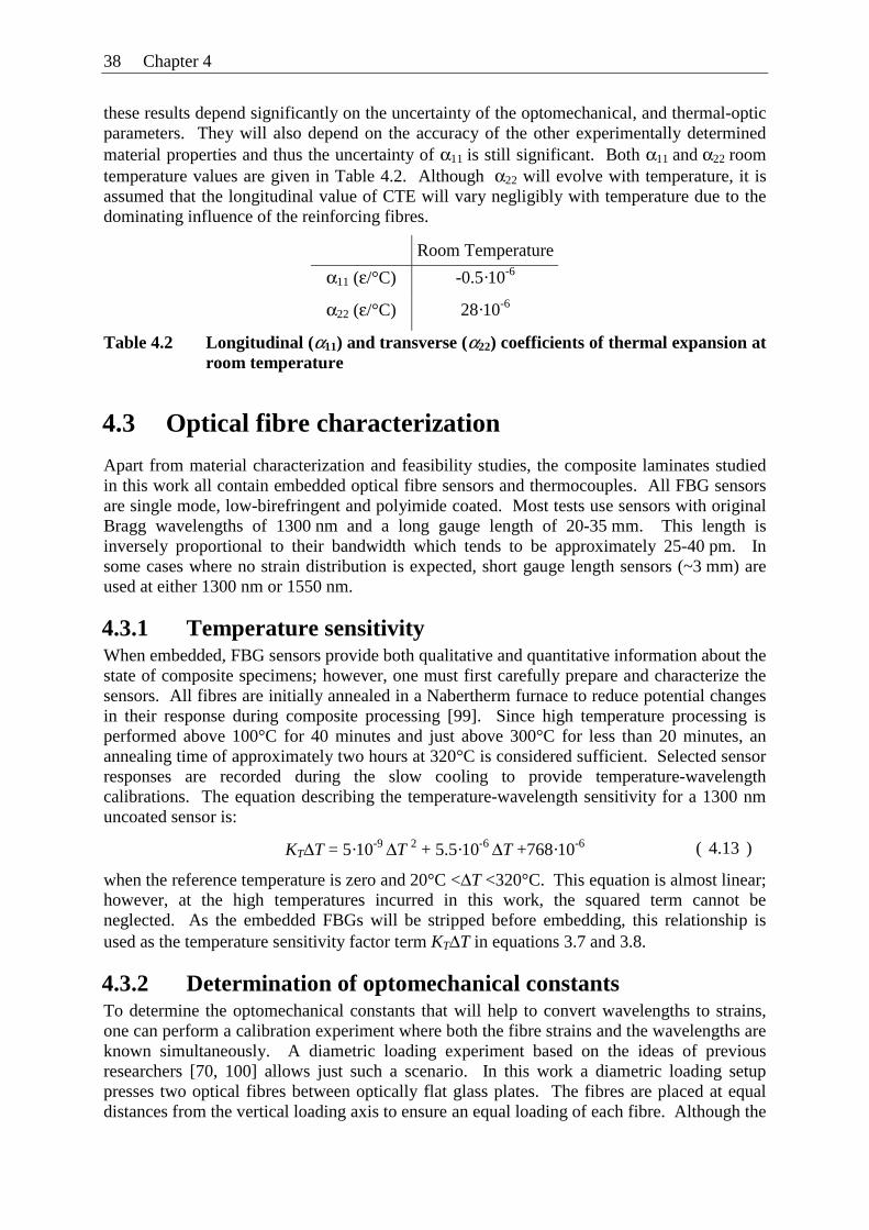
38 Chapter 4
these results depend significantly on the uncertainty of the optomechanical, and thermal-optic parameters. They will also depend on the accuracy of the other experimentally determined material properties and thus the uncertainty of α11 is still significant. Both α11 and α22 room temperature values are given in Table 4.2. Although α22 will evolve with temperature, it is assumed that the longitudinal value of CTE will vary negligibly with temperature due to the dominating influence of the reinforcing fibres.
Room Temperature
α11 (ε/°C) -0.5·10-6
α22 (ε/°C) 28·10-6
Table 4.2 Longitudinal (α11) and transverse (α22) coefficients of thermal expansion at room temperature
4.3 Optical fibre characterization
Apart from material characterization and feasibility studies, the composite laminates studied in this work all contain embedded optical fibre sensors and thermocouples. All FBG sensors are single mode, low-birefringent and polyimide coated. Most tests use sensors with original Bragg wavelengths of 1300 nm and a long gauge length of 20-35 mm. This length is inversely proportional to their bandwidth which tends to be approximately 25-40 pm. In some cases where no strain distribution is expected, short gauge length sensors (~3 mm) are used at either 1300 nm or 1550 nm.
4.3.1 Temperature sensitivity When embedded, FBG sensors provide both qualitative and quantitative information about the state of composite specimens; however, one must first carefully prepare and characterize the sensors. All fibres are initially annealed in a Nabertherm furnace to reduce potential changes in their response during composite processing [99]. Since high temperature processing is performed above 100°C for 40 minutes and just above 300°C for less than 20 minutes, an annealing time of approximately two hours at 320°C is considered sufficient. Selected sensor responses are recorded during the slow cooling to provide temperature-wavelength calibrations. The equation describing the temperature-wavelength sensitivity for a 1300 nm uncoated sensor is:
when the reference temperature is zero and 20°C <ΔT <320°C. This equation is almost linear; however, at the high temperatures incurred in this work, the squared term cannot be neglected. As the embedded FBGs will be stripped before embedding, this relationship is used as the temperature sensitivity factor term KTΔT in equations 3.7 and 3.8.
4.3.2 Determination of optomechanical constants To determine the optomechanical constants that will help to convert wavelengths to strains, one can perform a calibration experiment where both the fibre strains and the wavelengths are known simultaneously. A diametric loading experiment based on the ideas of previous researchers [70, 100] allows just such a scenario. In this work a diametric loading setup presses two optical fibres between optically flat glass plates. The fibres are placed at equal distances from the vertical loading axis to ensure an equal loading of each fibre. Although the
KTΔT = 5·10-9 ΔT 2 + 5.5·10-6 ΔT +768·10-6 ( 4.13 )
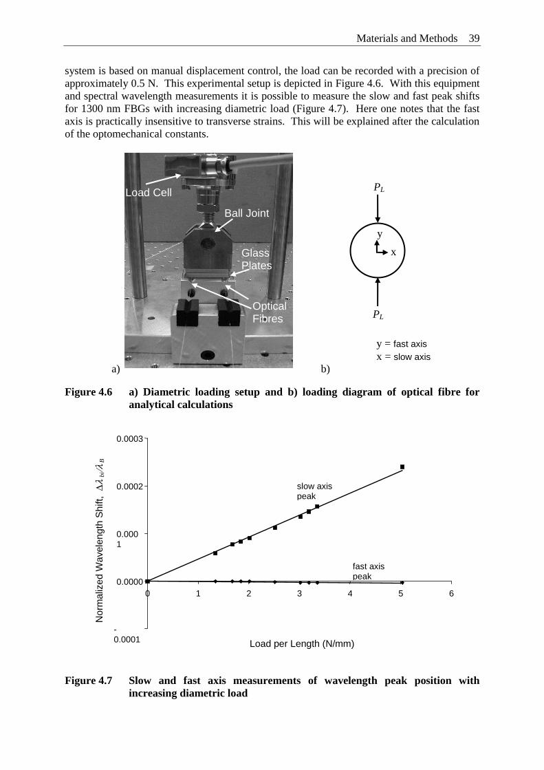
Materials and Methods 39
system is based on manual displacement control, the load can be recorded with a precision of approximately 0.5 N. This experimental setup is depicted in Figure 4.6. With this equipment and spectral wavelength measurements it is possible to measure the slow and fast peak shifts for 1300 nm FBGs with increasing diametric load (Figure 4.7). Here one notes that the fast axis is practically insensitive to transverse strains. This will be explained after the calculation of the optomechanical constants.
Figure 4.6 a) Diametric loading setup and b) loading diagram of optical fibre for analytical calculations
Figure 4.7 Slow and fast axis measurements of wavelength peak position with increasing diametric load
-0.0001
0.0000
0.0001
0.0002
0.0003
0 1 2 3 4 5 6
Load per Length (N/mm)
slow axis peak
fast axis peak
Nor
mal
ized
Wav
elen
gth
Shi
ft, Δ
λ bi
/λ B
y
x
PL
PL
y = fast axis x = slow axis
Optical Fibres
Load Cell
Ball Joint
Glass Plates
a) b)
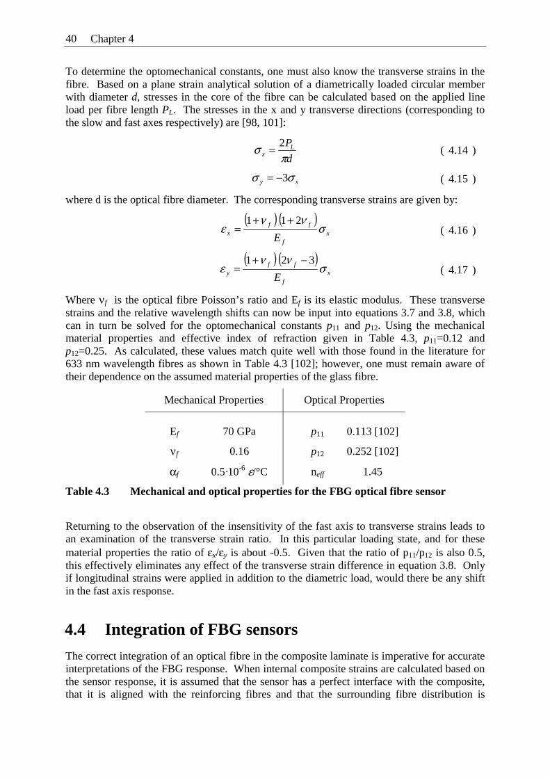
40 Chapter 4
To determine the optomechanical constants, one must also know the transverse strains in the fibre. Based on a plane strain analytical solution of a diametrically loaded circular member with diameter d, stresses in the core of the fibre can be calculated based on the applied line load per fibre length PL. The stresses in the x and y transverse directions (corresponding to the slow and fast axes respectively) are [98, 101]:
where d is the optical fibre diameter. The corresponding transverse strains are given by:
Where νf is the optical fibre Poisson’s ratio and Ef is its elastic modulus. These transverse strains and the relative wavelength shifts can now be input into equations 3.7 and 3.8, which can in turn be solved for the optomechanical constants p11 and p12. Using the mechanical material properties and effective index of refraction given in Table 4.3, p11=0.12 and p12=0.25. As calculated, these values match quite well with those found in the literature for 633 nm wavelength fibres as shown in Table 4.3 [102]; however, one must remain aware of their dependence on the assumed material properties of the glass fibre.
Mechanical Properties Optical Properties
Ef
70 GPa
p11
0.113 [102]
νf 0.16 p12 0.252 [102]
αf 0.5·10-6 ε/°C neff 1.45
Table 4.3 Mechanical and optical properties for the FBG optical fibre sensor
Returning to the observation of the insensitivity of the fast axis to transverse strains leads to an examination of the transverse strain ratio. In this particular loading state, and for these material properties the ratio of εx/εy is about -0.5. Given that the ratio of p11/p12 is also 0.5, this effectively eliminates any effect of the transverse strain difference in equation 3.8. Only if longitudinal strains were applied in addition to the diametric load, would there be any shift in the fast axis response.
4.4 Integration of FBG sensors
The correct integration of an optical fibre in the composite laminate is imperative for accurate interpretations of the FBG response. When internal composite strains are calculated based on the sensor response, it is assumed that the sensor has a perfect interface with the composite, that it is aligned with the reinforcing fibres and that the surrounding fibre distribution is
d
PLx π
σ 2= ( 4.14 )
xy σσ 3−= ( 4.15 )
( ) ( )
xf
ffx E
σνν
ε211 ++
= ( 4.16 )
( ) ( )
xf
ffy E
σνν
ε321 −+
= ( 4.17 )
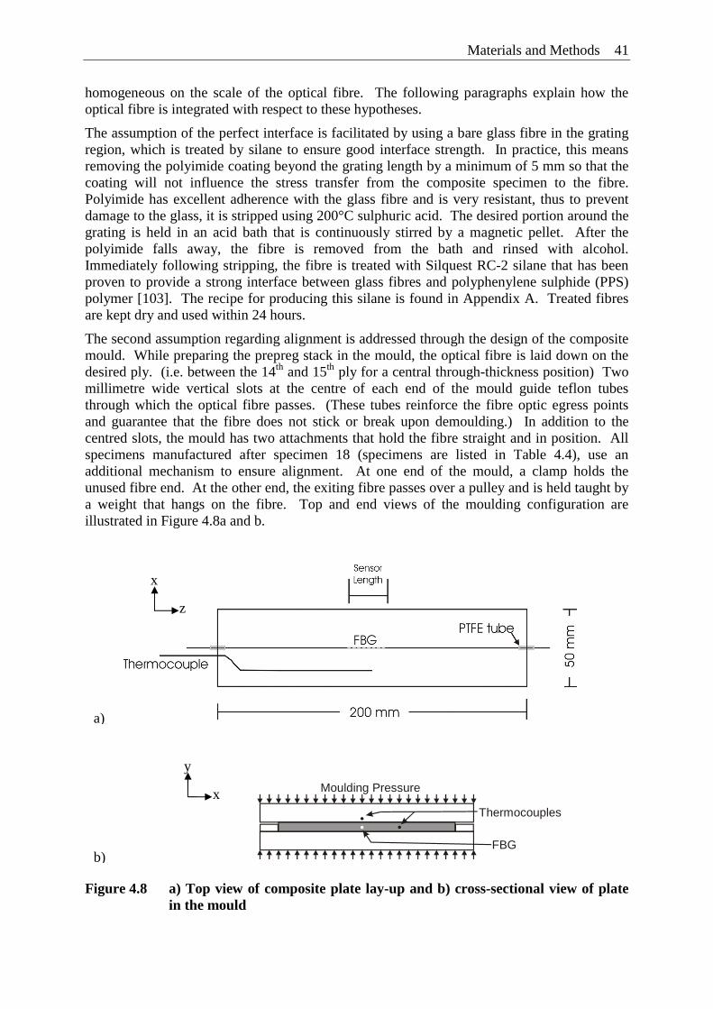
Materials and Methods 41
homogeneous on the scale of the optical fibre. The following paragraphs explain how the optical fibre is integrated with respect to these hypotheses.
The assumption of the perfect interface is facilitated by using a bare glass fibre in the grating region, which is treated by silane to ensure good interface strength. In practice, this means removing the polyimide coating beyond the grating length by a minimum of 5 mm so that the coating will not influence the stress transfer from the composite specimen to the fibre. Polyimide has excellent adherence with the glass fibre and is very resistant, thus to prevent damage to the glass, it is stripped using 200°C sulphuric acid. The desired portion around the grating is held in an acid bath that is continuously stirred by a magnetic pellet. After the polyimide falls away, the fibre is removed from the bath and rinsed with alcohol. Immediately following stripping, the fibre is treated with Silquest RC-2 silane that has been proven to provide a strong interface between glass fibres and polyphenylene sulphide (PPS) polymer [103]. The recipe for producing this silane is found in Appendix A. Treated fibres are kept dry and used within 24 hours.
The second assumption regarding alignment is addressed through the design of the composite mould. While preparing the prepreg stack in the mould, the optical fibre is laid down on the desired ply. (i.e. between the 14th and 15th ply for a central through-thickness position) Two millimetre wide vertical slots at the centre of each end of the mould guide teflon tubes through which the optical fibre passes. (These tubes reinforce the fibre optic egress points and guarantee that the fibre does not stick or break upon demoulding.) In addition to the centred slots, the mould has two attachments that hold the fibre straight and in position. All specimens manufactured after specimen 18 (specimens are listed in Table 4.4), use an additional mechanism to ensure alignment. At one end of the mould, a clamp holds the unused fibre end. At the other end, the exiting fibre passes over a pulley and is held taught by a weight that hangs on the fibre. Top and end views of the moulding configuration are illustrated in Figure 4.8a and b.
Figure 4.8 a) Top view of composite plate lay-up and b) cross-sectional view of plate in the mould
a)
Moulding Pressure
Thermocouples
y
x
x
z
b) FBG
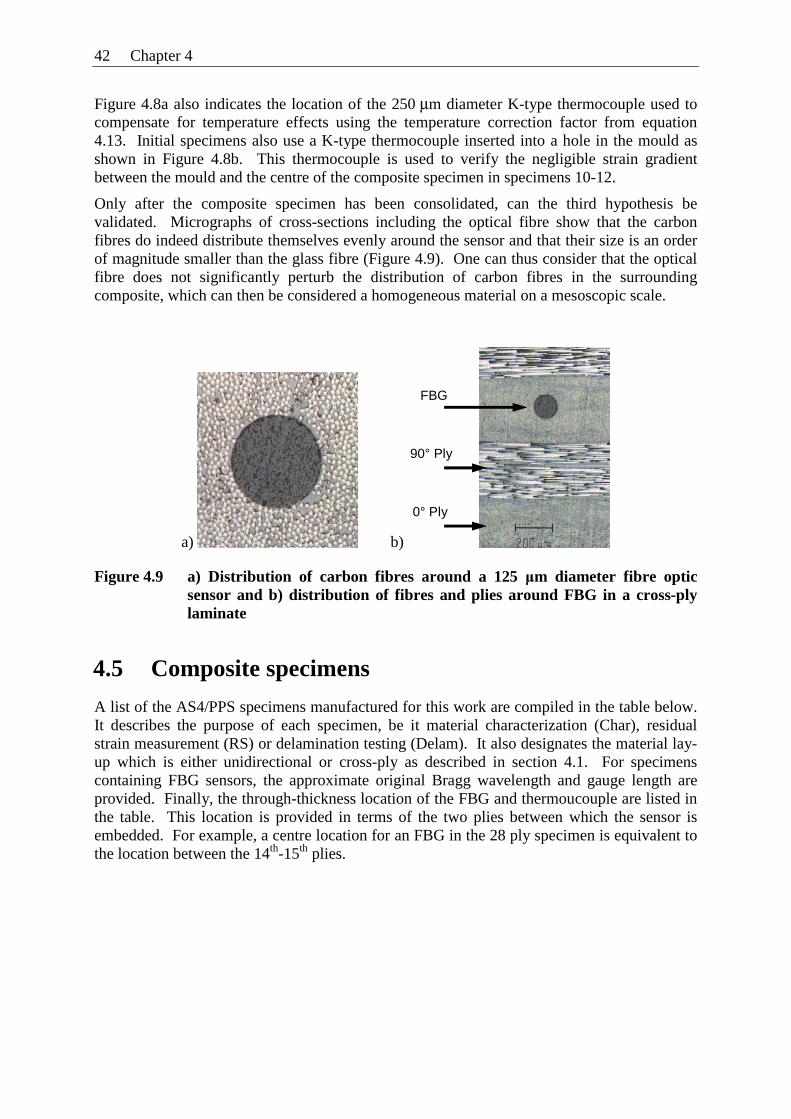
42 Chapter 4
Figure 4.8a also indicates the location of the 250 μm diameter K-type thermocouple used to compensate for temperature effects using the temperature correction factor from equation 4.13. Initial specimens also use a K-type thermocouple inserted into a hole in the mould as shown in Figure 4.8b. This thermocouple is used to verify the negligible strain gradient between the mould and the centre of the composite specimen in specimens 10-12.
Only after the composite specimen has been consolidated, can the third hypothesis be validated. Micrographs of cross-sections including the optical fibre show that the carbon fibres do indeed distribute themselves evenly around the sensor and that their size is an order of magnitude smaller than the glass fibre (Figure 4.9). One can thus consider that the optical fibre does not significantly perturb the distribution of carbon fibres in the surrounding composite, which can then be considered a homogeneous material on a mesoscopic scale.
a) b)
Figure 4.9 a) Distribution of carbon fibres around a 125 μm diameter fibre optic sensor and b) distribution of fibres and plies around FBG in a cross-ply laminate
4.5 Composite specimens
A list of the AS4/PPS specimens manufactured for this work are compiled in the table below. It describes the purpose of each specimen, be it material characterization (Char), residual strain measurement (RS) or delamination testing (Delam). It also designates the material lay-up which is either unidirectional or cross-ply as described in section 4.1. For specimens containing FBG sensors, the approximate original Bragg wavelength and gauge length are provided. Finally, the through-thickness location of the FBG and thermoucouple are listed in the table. This location is provided in terms of the two plies between which the sensor is embedded. For example, a centre location for an FBG in the 28 ply specimen is equivalent to the location between the 14th-15th plies.
90° Ply
FBG
0° Ply
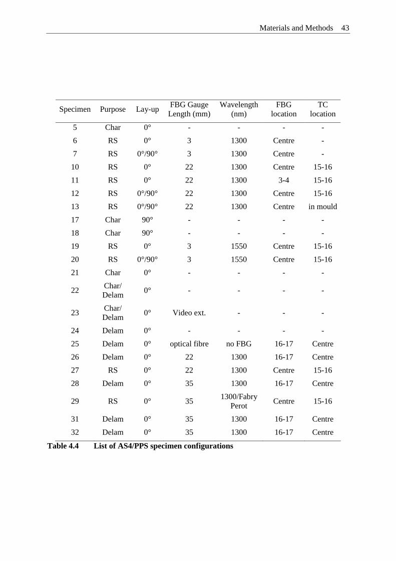
Materials and Methods 43
Specimen Purpose Lay-up FBG Gauge Length (mm)
Wavelength (nm)
FBG location
TC location
5 Char 0° - - - -
6 RS 0° 3 1300 Centre -
7 RS 0°/90° 3 1300 Centre -
10 RS 0° 22 1300 Centre 15-16
11 RS 0° 22 1300 3-4 15-16
12 RS 0°/90° 22 1300 Centre 15-16
13 RS 0°/90° 22 1300 Centre in mould
17 Char 90° - - - -
18 Char 90° - - - -
19 RS 0° 3 1550 Centre 15-16
20 RS 0°/90° 3 1550 Centre 15-16
21 Char 0° - - - -
22 Char/ Delam
0° - - - -
23 Char/ Delam
0° Video ext. - - -
24 Delam 0° - - - -
25 Delam 0° optical fibre no FBG 16-17 Centre
26 Delam 0° 22 1300 16-17 Centre
27 RS 0° 22 1300 Centre 15-16
28 Delam 0° 35 1300 16-17 Centre
29 RS 0° 35 1300/Fabry
Perot Centre 15-16
31 Delam 0° 35 1300 16-17 Centre
32 Delam 0° 35 1300 16-17 Centre
Table 4.4 List of AS4/PPS specimen configurations

Chapter 5 Residual Strains
During production, a three-dimensional state of residual stresses and strains accumulates in composite materials. Each type of material, each set of processing parameters and each laminate stacking sequence will create a specific internal residual stress state that will in turn dictate the performance of the composite structure. In some cases, one may wish to optimize these internal stresses to increase ultimate static strength or fatigue resistance or to eliminate premature damage such as microcracking. It may also be helpful to understand the initial internal strain state when considering the response of a composite structure to applied external loads or to in-service damage.
In this chapter fibre Bragg gratings are used to understand how the three-dimensional residual strains accumulate in composites during processing. Although strains along the length of the long composite specimen investigated here tend to be uniform, the sensors are subjected to unequal transverse strains, which can both add to the understanding of the process and can complicate the interpretation of FBG readings. Measurements of Bragg wavelength spectra provide a basis for the discussion of material changes during processing and of the final strain state. Numerical analysis of the consolidation process is included to improve the understanding of strain development and is used to discuss the influence of specimen-tool interaction. Numerical modelling also simulates the stresses and strains that can be expected in the composite material away from the FBG sensor. Given the complexity of the specimen-tool interaction, material behaviour and ultimately the significant transverse strains, it is shown that significant error can be incurred by making traditional assumptions about strain-wavelength relationships.
5.1 Experimental overview
To measure residual strain accumulation due to processing, unidirectional and cross-ply AS4/PPS laminates are prepared according to the procedure outlined in the previous chapter and illustrated in Figure 4.8. Unidirectional specimens destined for delamination testing (see section 6.1.1) are also included in this study, despite the rectangular piece of aluminium foil inserted between the centre plies at one end of the specimen. Examination of the results indicates that these specimens follow the same accumulation of residual strains as unidirectional specimens without an aluminium insert.
Due to the longitudinal uniformity of the strains that accumulate in the centre of the composite specimens during consolidation, this study can be accomplished solely with spectral amplitude measurements. Specifically, measurements of wavelength peak positions are taken before, during and after production. For long gauge length sensors, complete spectra are recorded to provide information about birefringence during and after processing. In practice, the full spectrum responses are acquired with a photodetector coupled to a tuneable laser. A data logging system provides concurrent temperature acquisition for the thermocouples as shown in Figure 5.1.
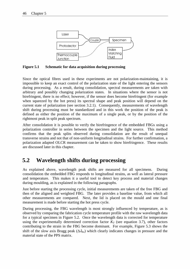
46 Chapter 5
Figure 5.1 Schematic for data acquisition during processing
Since the optical fibres used in these experiments are not polarization-maintaining, it is impossible to keep an exact control of the polarization state of the light entering the sensors during processing. As a result, during consolidation, spectral measurements are taken with arbitrary and possibly changing polarization states. In situations where the sensor is not birefringent, there is no effect; however, if the sensor does become birefringent (for example when squeezed by the hot press) its spectral shape and peak position will depend on the current state of polarization (see section 3.2.1). Consequently, measurements of wavelength shift during processing must be standardized and in this work the position of the peak is defined as either the position of the maximum of a single peak, or by the position of the rightmost peak in split peak spectrum.
After consolidation it is possible to verify the birefringence of the embedded FBGs using a polarization controller in series between the specimen and the light source. This method confirms that the peak splits observed during consolidation are the result of unequal transverse strains and not that of non-uniform longitudinal strains. For further confirmation, a polarization adapted OLCR measurement can be taken to show birefringence. These results are discussed later in this chapter.
5.2 Wavelength shifts during processing
As explained above, wavelength peak shifts are measured for all specimens. During consolidation the embedded FBG responds to longitudinal strains, as well as lateral pressure and temperature. This makes it a useful tool to detect key process and material changes during moulding, as is explained in the following paragraphs.
Just before starting the processing cycle, initial measurements are taken of the free FBG and then of the aligned and weighted FBG. The later provides a baseline value, from which all other measurements are compared. Next, the lid is placed on the mould and one final measurement is made before starting the hot press cycle.
During processing, the FBG wavelength is most strongly influenced by temperature, as is observed by comparing the fabrication cycle temperature profile with the raw wavelength data for a typical specimen in Figure 5.2. Once the wavelength data is corrected for temperature using the experimentally determined correction factor KT (see equation 3.7), other factors contributing to the strain in the FBG become dominant. For example, Figure 5.3 shows the shift of the slow axis Bragg peak (Δλbx) which clearly indicates changes in pressure and the material state of the PPS matrix.
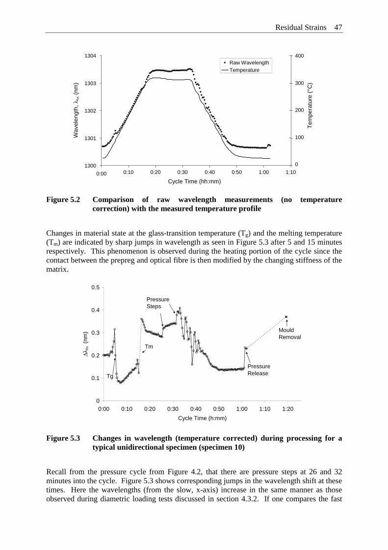
Residual Strains 47
Figure 5.2 Comparison of raw wavelength measurements (no temperature correction) with the measured temperature profile
Changes in material state at the glass-transition temperature (Tg) and the melting temperature (Tm) are indicated by sharp jumps in wavelength as seen in Figure 5.3 after 5 and 15 minutes respectively. This phenomenon is observed during the heating portion of the cycle since the contact between the prepreg and optical fibre is then modified by the changing stiffness of the matrix.
0
0.1
0.2
0.3
0.4
0.5
0:00 0:10 0:20 0:30 0:40 0:50 1:00 1:10 1:20
Cycle Time (h:mm)
Δλbx
(nm
)
Tg
Tm
PressureSteps
PressureRelease
Mould Removal
Figure 5.3 Changes in wavelength (temperature corrected) during processing for a typical unidirectional specimen (specimen 10)
Recall from the pressure cycle from Figure 4.2, that there are pressure steps at 26 and 32 minutes into the cycle. Figure 5.3 shows corresponding jumps in the wavelength shift at these times. Here the wavelengths (from the slow, x-axis) increase in the same manner as those observed during diametric loading tests discussed in section 4.3.2. If one compares the fast
1300
1301
1302
1303
1304
0:00 0:10 0:20 0:30 0:40 0:50 1:00 1:10 Cycle Time (hh:mm)
Wav
elen
gth,
λbx
(nm
)
0
100
200
300
400
Tem
pera
ture
(°C
)
Raw Wavelength Temperature
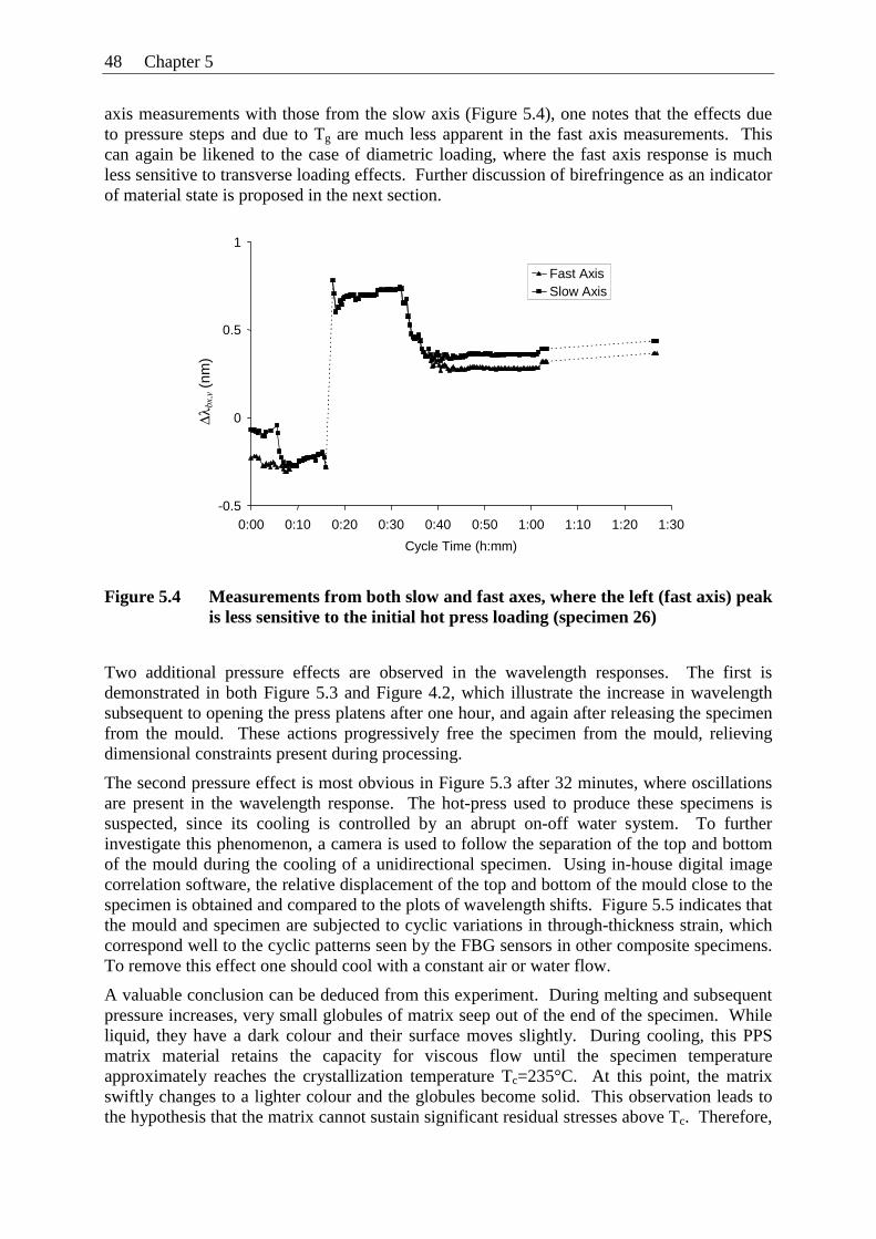
48 Chapter 5
axis measurements with those from the slow axis (Figure 5.4), one notes that the effects due to pressure steps and due to Tg are much less apparent in the fast axis measurements. This can again be likened to the case of diametric loading, where the fast axis response is much less sensitive to transverse loading effects. Further discussion of birefringence as an indicator of material state is proposed in the next section.
Figure 5.4 Measurements from both slow and fast axes, where the left (fast axis) peak is less sensitive to the initial hot press loading (specimen 26)
Two additional pressure effects are observed in the wavelength responses. The first is demonstrated in both Figure 5.3 and Figure 4.2, which illustrate the increase in wavelength subsequent to opening the press platens after one hour, and again after releasing the specimen from the mould. These actions progressively free the specimen from the mould, relieving dimensional constraints present during processing.
The second pressure effect is most obvious in Figure 5.3 after 32 minutes, where oscillations are present in the wavelength response. The hot-press used to produce these specimens is suspected, since its cooling is controlled by an abrupt on-off water system. To further investigate this phenomenon, a camera is used to follow the separation of the top and bottom of the mould during the cooling of a unidirectional specimen. Using in-house digital image correlation software, the relative displacement of the top and bottom of the mould close to the specimen is obtained and compared to the plots of wavelength shifts. Figure 5.5 indicates that the mould and specimen are subjected to cyclic variations in through-thickness strain, which correspond well to the cyclic patterns seen by the FBG sensors in other composite specimens. To remove this effect one should cool with a constant air or water flow.
A valuable conclusion can be deduced from this experiment. During melting and subsequent pressure increases, very small globules of matrix seep out of the end of the specimen. While liquid, they have a dark colour and their surface moves slightly. During cooling, this PPS matrix material retains the capacity for viscous flow until the specimen temperature approximately reaches the crystallization temperature Tc=235°C. At this point, the matrix swiftly changes to a lighter colour and the globules become solid. This observation leads to the hypothesis that the matrix cannot sustain significant residual stresses above Tc. Therefore,
-0.5
0
0.5
1
0:00 0:10 0:20 0:30 0:40 0:50 1:00 1:10 1:20 1:30
Cycle Time (h:mm)
Δλbx
,y (
nm)
Fast AxisSlow Axis
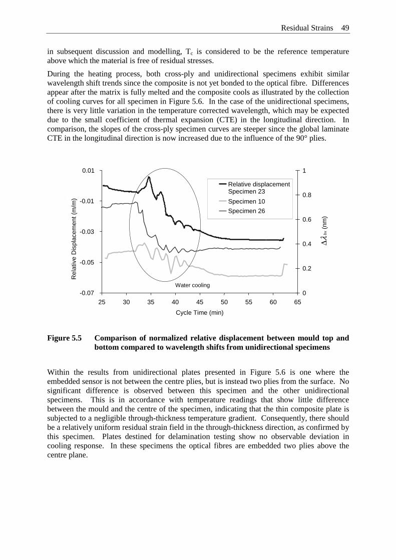
Residual Strains 49
in subsequent discussion and modelling, Tc is considered to be the reference temperature above which the material is free of residual stresses.
During the heating process, both cross-ply and unidirectional specimens exhibit similar wavelength shift trends since the composite is not yet bonded to the optical fibre. Differences appear after the matrix is fully melted and the composite cools as illustrated by the collection of cooling curves for all specimen in Figure 5.6. In the case of the unidirectional specimens, there is very little variation in the temperature corrected wavelength, which may be expected due to the small coefficient of thermal expansion (CTE) in the longitudinal direction. In comparison, the slopes of the cross-ply specimen curves are steeper since the global laminate CTE in the longitudinal direction is now increased due to the influence of the 90° plies.
Figure 5.5 Comparison of normalized relative displacement between mould top and bottom compared to wavelength shifts from unidirectional specimens
Within the results from unidirectional plates presented in Figure 5.6 is one where the embedded sensor is not between the centre plies, but is instead two plies from the surface. No significant difference is observed between this specimen and the other unidirectional specimens. This is in accordance with temperature readings that show little difference between the mould and the centre of the specimen, indicating that the thin composite plate is subjected to a negligible through-thickness temperature gradient. Consequently, there should be a relatively uniform residual strain field in the through-thickness direction, as confirmed by this specimen. Plates destined for delamination testing show no observable deviation in cooling response. In these specimens the optical fibres are embedded two plies above the centre plane.
-0.07
-0.05
-0.03
-0.01
0.01
25 30 35 40 45 50 55 60 65
Cycle Time (min)
Rel
ativ
e D
ispl
acem
ent (
m/m
)
0
0.2
0.4
0.6
0.8
1
Δλ b
x (n
m)
(nm
)
Relative displacement Specimen 23
Specimen 10
Specimen 26
Water cooling
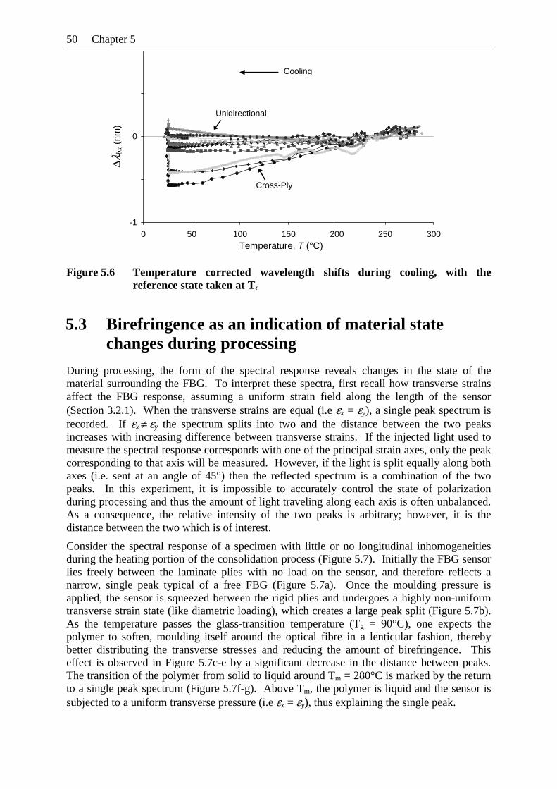
50 Chapter 5
Figure 5.6 Temperature corrected wavelength shifts during cooling, with the reference state taken at Tc
5.3 Birefringence as an indication of material state changes during processing
During processing, the form of the spectral response reveals changes in the state of the material surrounding the FBG. To interpret these spectra, first recall how transverse strains affect the FBG response, assuming a uniform strain field along the length of the sensor (Section 3.2.1). When the transverse strains are equal (i.e εx = εy), a single peak spectrum is recorded. If εx ≠ εy the spectrum splits into two and the distance between the two peaks increases with increasing difference between transverse strains. If the injected light used to measure the spectral response corresponds with one of the principal strain axes, only the peak corresponding to that axis will be measured. However, if the light is split equally along both axes (i.e. sent at an angle of 45°) then the reflected spectrum is a combination of the two peaks. In this experiment, it is impossible to accurately control the state of polarization during processing and thus the amount of light traveling along each axis is often unbalanced. As a consequence, the relative intensity of the two peaks is arbitrary; however, it is the distance between the two which is of interest.
Consider the spectral response of a specimen with little or no longitudinal inhomogeneities during the heating portion of the consolidation process (Figure 5.7). Initially the FBG sensor lies freely between the laminate plies with no load on the sensor, and therefore reflects a narrow, single peak typical of a free FBG (Figure 5.7a). Once the moulding pressure is applied, the sensor is squeezed between the rigid plies and undergoes a highly non-uniform transverse strain state (like diametric loading), which creates a large peak split (Figure 5.7b). As the temperature passes the glass-transition temperature (Tg = 90°C), one expects the polymer to soften, moulding itself around the optical fibre in a lenticular fashion, thereby better distributing the transverse stresses and reducing the amount of birefringence. This effect is observed in Figure 5.7c-e by a significant decrease in the distance between peaks. The transition of the polymer from solid to liquid around Tm = 280°C is marked by the return to a single peak spectrum (Figure 5.7f-g). Above Tm, the polymer is liquid and the sensor is subjected to a uniform transverse pressure (i.e εx = εy), thus explaining the single peak.
-1
0
0 50 100 150 200 250 300Temperature (°C)
Δλb (
nm)
Cooling
Cross-Ply
UnidirectionalΔλ
bx (n
m)
Temperature, T (°C)
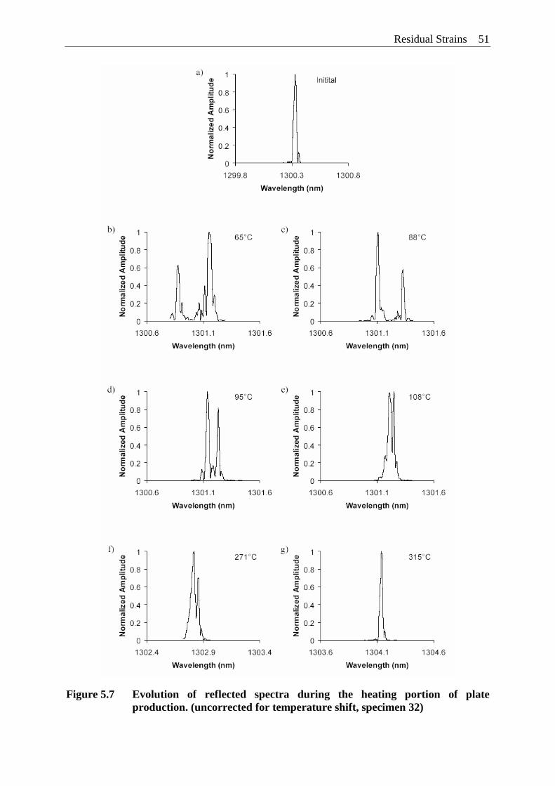
Residual Strains 51
Figure 5.7 Evolution of reflected spectra during the heating portion of plate production. (uncorrected for temperature shift, specimen 32)
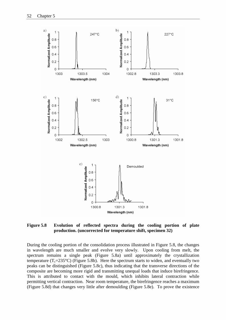
52 Chapter 5
Figure 5.8 Evolution of reflected spectra during the cooling portion of plate production. (uncorrected for temperature shift, specimen 32)
During the cooling portion of the consolidation process illustrated in Figure 5.8, the changes in wavelength are much smaller and evolve very slowly. Upon cooling from melt, the spectrum remains a single peak (Figure 5.8a) until approximately the crystallization temperature (Tc=235°C) (Figure 5.8b). Here the spectrum starts to widen, and eventually two peaks can be distinguished (Figure 5.8c), thus indicating that the transverse directions of the composite are becoming more rigid and transmitting unequal loads that induce birefringence. This is attributed to contact with the mould, which inhibits lateral contraction while permitting vertical contraction. Near room temperature, the birefringence reaches a maximum (Figure 5.8d) that changes very little after demoulding (Figure 5.8e). To prove the existence
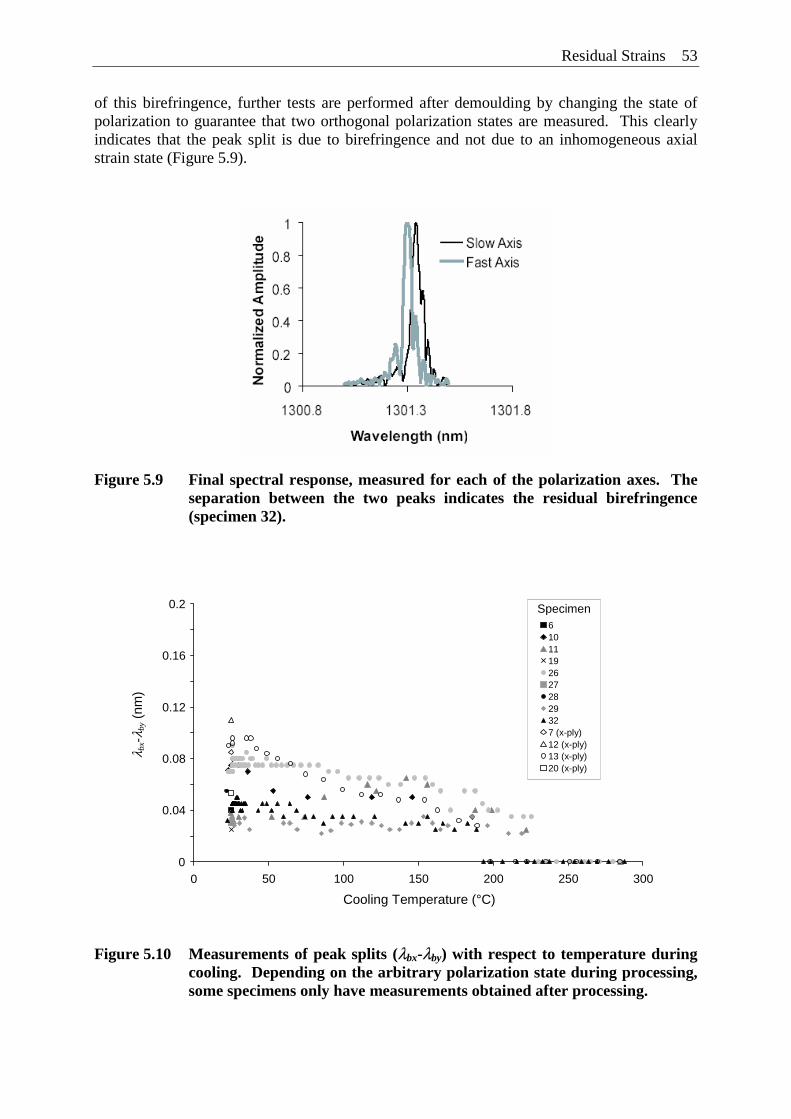
Residual Strains 53
of this birefringence, further tests are performed after demoulding by changing the state of polarization to guarantee that two orthogonal polarization states are measured. This clearly indicates that the peak split is due to birefringence and not due to an inhomogeneous axial strain state (Figure 5.9).
Figure 5.9 Final spectral response, measured for each of the polarization axes. The separation between the two peaks indicates the residual birefringence (specimen 32).
Figure 5.10 Measurements of peak splits (λbx-λby) with respect to temperature during cooling. Depending on the arbitrary polarization state during processing, some specimens only have measurements obtained after processing.
0
0.04
0.08
0.12
0.16
0.2
0 50 100 150 200 250 300
Cooling Temperature (°C)
λ bx-
λ by (
nm)
6 10 11 19 26 27 28 29 32 7 (x-ply) 12 (x-ply) 13 (x-ply) 20 (x-ply)
Specimen
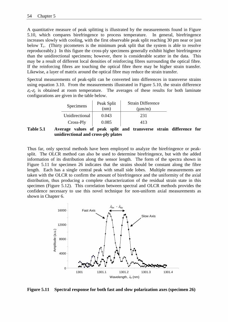
54 Chapter 5
A quantitative measure of peak splitting is illustrated by the measurements found in Figure 5.10, which compares birefringence to process temperature. In general, birefringence increases slowly with cooling, with the first observable peak split reaching 30 pm near or just below Tc. (Thirty picometers is the minimum peak split that the system is able to resolve reproduceably.) In this figure the cross-ply specimens generally exhibit higher birefringence than the unidirectional specimens; however, there is considerable scatter in the data. This may be a result of different local densities of reinforcing fibres surrounding the optical fibre. If the reinforcing fibres are touching the optical fibre there may be higher strain transfer. Likewise, a layer of matrix around the optical fibre may reduce the strain transfer.
Spectral measurements of peak-split can be converted into differences in transverse strains using equation 3.10. From the measurements illustrated in Figure 5.10, the strain difference εx-εy is obtained at room temperature. The averages of these results for both laminate configurations are given in the table below.
Specimens Peak Split
(nm) Strain Difference
(μm/m)
Unidirectional 0.043 231
Cross-Ply 0.085 413
Table 5.1 Average values of peak split and transverse strain difference for unidirectional and cross-ply plates
Thus far, only spectral methods have been employed to analyze the birefringence or peak-split. The OLCR method can also be used to determine birefringence, but with the added information of its distribution along the sensor length. The form of the spectra shown in Figure 5.11 for specimen 26 indicates that the strains should be constant along the fibre length. Each has a single central peak with small side lobes. Multiple measurements are taken with the OLCR to confirm the amount of birefringence and the uniformity of the axial distribution, thus producing a complete characterization of the residual strain state in this specimen (Figure 5.12). This correlation between spectral and OLCR methods provides the confidence necessary to use this novel technique for non-uniform axial measurements as shown in Chapter 6.
Figure 5.11 Spectral response for both fast and slow polarization axes (specimen 26)
0
4000
8000
12000
16000
1301 1301.1 1301.2 1301.3 1301.4
Wavelength, λb (nm)
Am
plitu
de (
a.u.
)
Slow Axis
Fast Axis λbx - λby
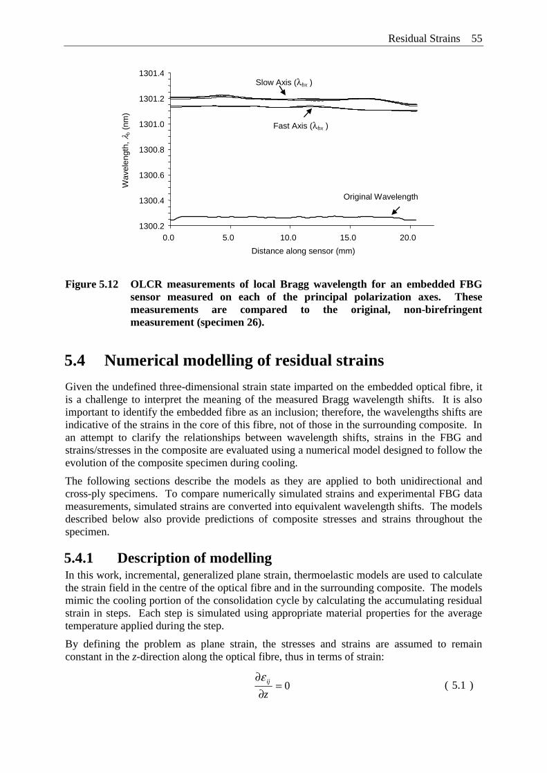
Residual Strains 55
Figure 5.12 OLCR measurements of local Bragg wavelength for an embedded FBG sensor measured on each of the principal polarization axes. These measurements are compared to the original, non-birefringent measurement (specimen 26).
5.4 Numerical modelling of residual strains
Given the undefined three-dimensional strain state imparted on the embedded optical fibre, it is a challenge to interpret the meaning of the measured Bragg wavelength shifts. It is also important to identify the embedded fibre as an inclusion; therefore, the wavelengths shifts are indicative of the strains in the core of this fibre, not of those in the surrounding composite. In an attempt to clarify the relationships between wavelength shifts, strains in the FBG and strains/stresses in the composite are evaluated using a numerical model designed to follow the evolution of the composite specimen during cooling.
The following sections describe the models as they are applied to both unidirectional and cross-ply specimens. To compare numerically simulated strains and experimental FBG data measurements, simulated strains are converted into equivalent wavelength shifts. The models described below also provide predictions of composite stresses and strains throughout the specimen.
5.4.1 Description of modelling In this work, incremental, generalized plane strain, thermoelastic models are used to calculate the strain field in the centre of the optical fibre and in the surrounding composite. The models mimic the cooling portion of the consolidation cycle by calculating the accumulating residual strain in steps. Each step is simulated using appropriate material properties for the average temperature applied during the step.
By defining the problem as plane strain, the stresses and strains are assumed to remain constant in the z-direction along the optical fibre, thus in terms of strain:
0=∂
∂zijε
( 5.1 )
1300.2
1300.4
1300.6
1300.8
1301.0
1301.2
1301.4
0.0 5.0 10.0 15.0 20.0 Distance along sensor (mm)
Wav
elen
gth,
λb
(nm
)
Original Wavelength Distribution
Slow Axis (λbx )
Fast Axis (λbx )
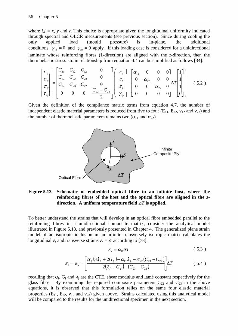
56 Chapter 5
where i,j = x, y and z. This choice is appropriate given the longitudinal uniformity indicated through spectral and OLCR measurements (see previous section). Since during cooling the only applied load (mould pressure) is in-plane, the additional conditions, 0and0 == xzyz γγ apply. If this loading case is considered for a unidirectional
laminate whose reinforcing fibres (1-direction) are aligned with the z-direction, then the thermoelastic stress-strain relationship from equation 4.4 can be simplified as follows [34]:
Given the definition of the compliance matrix terms from equation 4.7, the number of independent elastic material parameters is reduced from five to four (E11, E22, ν12 and ν23) and the number of thermoelastic parameters remains two (α11 and α22).
Figure 5.13 Schematic of embedded optical fibre in an infinite host, where the reinforcing fibres of the host and the optical fibre are aligned in the z-direction. A uniform temperature field ΔT is applied.
To better understand the strains that will develop in an optical fibre embedded parallel to the reinforcing fibres in a unidirectional composite matrix, consider the analytical model illustrated in Figure 5.13, and previously presented in Chapter 4. The generalized plane strain model of an isotropic inclusion in an infinite transversely isotropic matrix calculates the longitudinal εz and transverse strains εx = εy according to [78]:
recalling that αf, Gf and λf are the CTE, shear modulus and lamé constant respectively for the glass fibre. By examining the required composite parameters C22 and C23 in the above equations, it is observed that this formulation relies on the same four elastic material properties (E11, E22, ν12 and ν23) given above. Strains calculated using this analytical model will be compared to the results for the unidirectional specimen in the next section.
⎟⎟⎟⎟⎟
⎠
⎞
⎜⎜⎜⎜⎜
⎝
⎛
⎥⎥⎥⎥
⎦
⎤
⎢⎢⎢⎢
⎣
⎡
Δ
⎥⎥⎥⎥
⎦
⎤
⎢⎢⎢⎢
⎣
⎡
−
⎥⎥⎥⎥⎥
⎦
⎤
⎢⎢⎢⎢⎢
⎣
⎡
⎥⎥⎥⎥⎥
⎦
⎤
⎢⎢⎢⎢⎢
⎣
⎡
−=
⎥⎥⎥⎥⎥
⎦
⎤
⎢⎢⎢⎢⎢
⎣
⎡
0
1
1
1
0000
000
000
000
2000
0
0
0
22
22
11
2322
222312
232212
121211
T
CCCCC
CCC
CCC
xy
y
x
z
xy
y
x
z
αα
α
γεεε
τσσσ
( 5.2 )
Tz Δ= 11αε ( 5.3 )
( ) ( )
( ) ( ) TCCG
CCG
ff
ffffyx Δ
⎥⎥⎦
⎤
⎢⎢⎣
⎡
−−+−−−+
==2223
22232211
2
23
λαλαλα
εε ( 5.4 )
Optical Fibre
Infinite Composite Ply x
y
z ΔT
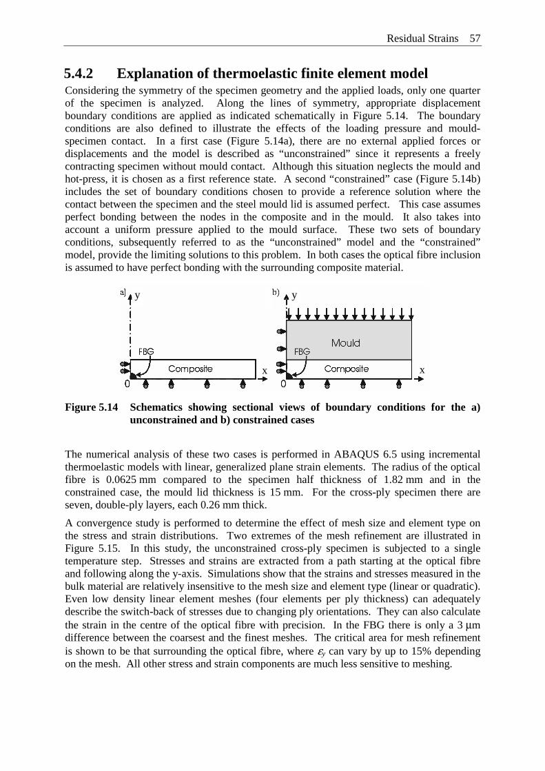
Residual Strains 57
5.4.2 Explanation of thermoelastic finite element model Considering the symmetry of the specimen geometry and the applied loads, only one quarter of the specimen is analyzed. Along the lines of symmetry, appropriate displacement boundary conditions are applied as indicated schematically in Figure 5.14. The boundary conditions are also defined to illustrate the effects of the loading pressure and mould-specimen contact. In a first case (Figure 5.14a), there are no external applied forces or displacements and the model is described as “unconstrained” since it represents a freely contracting specimen without mould contact. Although this situation neglects the mould and hot-press, it is chosen as a first reference state. A second “constrained” case (Figure 5.14b) includes the set of boundary conditions chosen to provide a reference solution where the contact between the specimen and the steel mould lid is assumed perfect. This case assumes perfect bonding between the nodes in the composite and in the mould. It also takes into account a uniform pressure applied to the mould surface. These two sets of boundary conditions, subsequently referred to as the “unconstrained” model and the “constrained” model, provide the limiting solutions to this problem. In both cases the optical fibre inclusion is assumed to have perfect bonding with the surrounding composite material.
Figure 5.14 Schematics showing sectional views of boundary conditions for the a) unconstrained and b) constrained cases
The numerical analysis of these two cases is performed in ABAQUS 6.5 using incremental thermoelastic models with linear, generalized plane strain elements. The radius of the optical fibre is 0.0625 mm compared to the specimen half thickness of 1.82 mm and in the constrained case, the mould lid thickness is 15 mm. For the cross-ply specimen there are seven, double-ply layers, each 0.26 mm thick.
A convergence study is performed to determine the effect of mesh size and element type on the stress and strain distributions. Two extremes of the mesh refinement are illustrated in Figure 5.15. In this study, the unconstrained cross-ply specimen is subjected to a single temperature step. Stresses and strains are extracted from a path starting at the optical fibre and following along the y-axis. Simulations show that the strains and stresses measured in the bulk material are relatively insensitive to the mesh size and element type (linear or quadratic). Even low density linear element meshes (four elements per ply thickness) can adequately describe the switch-back of stresses due to changing ply orientations. They can also calculate the strain in the centre of the optical fibre with precision. In the FBG there is only a 3 μm difference between the coarsest and the finest meshes. The critical area for mesh refinement is shown to be that surrounding the optical fibre, where εy can vary by up to 15% depending on the mesh. All other stress and strain components are much less sensitive to meshing.
y y
x x
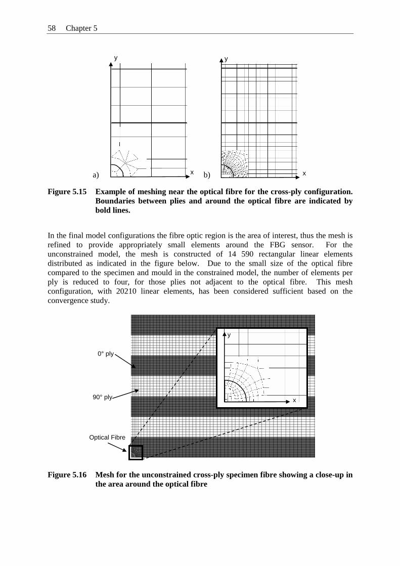
58 Chapter 5
Figure 5.15 Example of meshing near the optical fibre for the cross-ply configuration. Boundaries between plies and around the optical fibre are indicated by bold lines.
In the final model configurations the fibre optic region is the area of interest, thus the mesh is refined to provide appropriately small elements around the FBG sensor. For the unconstrained model, the mesh is constructed of 14 590 rectangular linear elements distributed as indicated in the figure below. Due to the small size of the optical fibre compared to the specimen and mould in the constrained model, the number of elements per ply is reduced to four, for those plies not adjacent to the optical fibre. This mesh configuration, with 20210 linear elements, has been considered sufficient based on the convergence study.
Figure 5.16 Mesh for the unconstrained cross-ply specimen fibre showing a close-up in the area around the optical fibre
0° ply
90° ply
Optical Fibre
y
x
a) b)
y
x
y
x
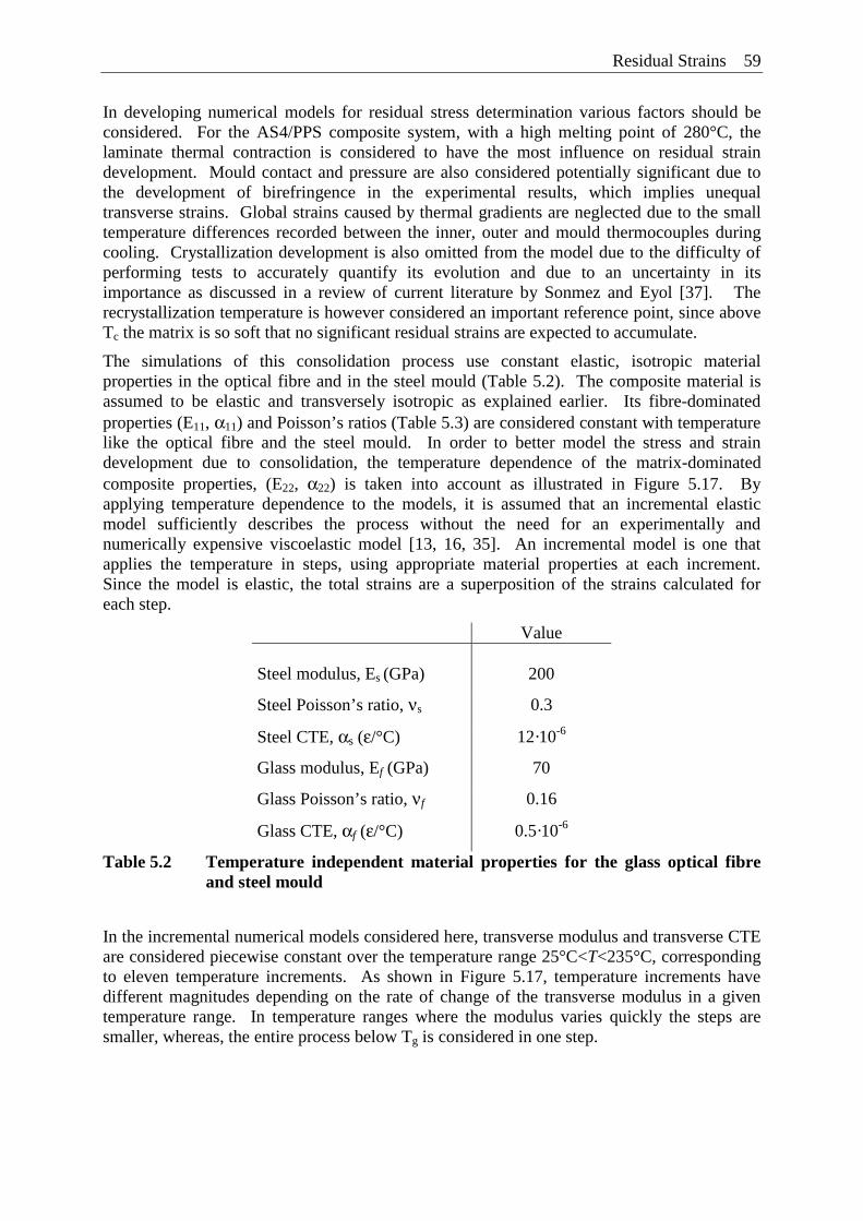
Residual Strains 59
In developing numerical models for residual stress determination various factors should be considered. For the AS4/PPS composite system, with a high melting point of 280°C, the laminate thermal contraction is considered to have the most influence on residual strain development. Mould contact and pressure are also considered potentially significant due to the development of birefringence in the experimental results, which implies unequal transverse strains. Global strains caused by thermal gradients are neglected due to the small temperature differences recorded between the inner, outer and mould thermocouples during cooling. Crystallization development is also omitted from the model due to the difficulty of performing tests to accurately quantify its evolution and due to an uncertainty in its importance as discussed in a review of current literature by Sonmez and Eyol [37]. The recrystallization temperature is however considered an important reference point, since above Tc the matrix is so soft that no significant residual strains are expected to accumulate.
The simulations of this consolidation process use constant elastic, isotropic material properties in the optical fibre and in the steel mould (Table 5.2). The composite material is assumed to be elastic and transversely isotropic as explained earlier. Its fibre-dominated properties (E11, α11) and Poisson’s ratios (Table 5.3) are considered constant with temperature like the optical fibre and the steel mould. In order to better model the stress and strain development due to consolidation, the temperature dependence of the matrix-dominated composite properties, (E22, α22) is taken into account as illustrated in Figure 5.17. By applying temperature dependence to the models, it is assumed that an incremental elastic model sufficiently describes the process without the need for an experimentally and numerically expensive viscoelastic model [13, 16, 35]. An incremental model is one that applies the temperature in steps, using appropriate material properties at each increment. Since the model is elastic, the total strains are a superposition of the strains calculated for each step.
Value Steel modulus, Es (GPa)
200
Steel Poisson’s ratio, νs 0.3
Steel CTE, αs (ε/°C) 12·10-6
Glass modulus, Ef (GPa) 70
Glass Poisson’s ratio, νf 0.16
Glass CTE, αf (ε/°C) 0.5·10-6
Table 5.2 Temperature independent material properties for the glass optical fibre and steel mould
In the incremental numerical models considered here, transverse modulus and transverse CTE are considered piecewise constant over the temperature range 25°C<T<235°C, corresponding to eleven temperature increments. As shown in Figure 5.17, temperature increments have different magnitudes depending on the rate of change of the transverse modulus in a given temperature range. In temperature ranges where the modulus varies quickly the steps are smaller, whereas, the entire process below Tg is considered in one step.
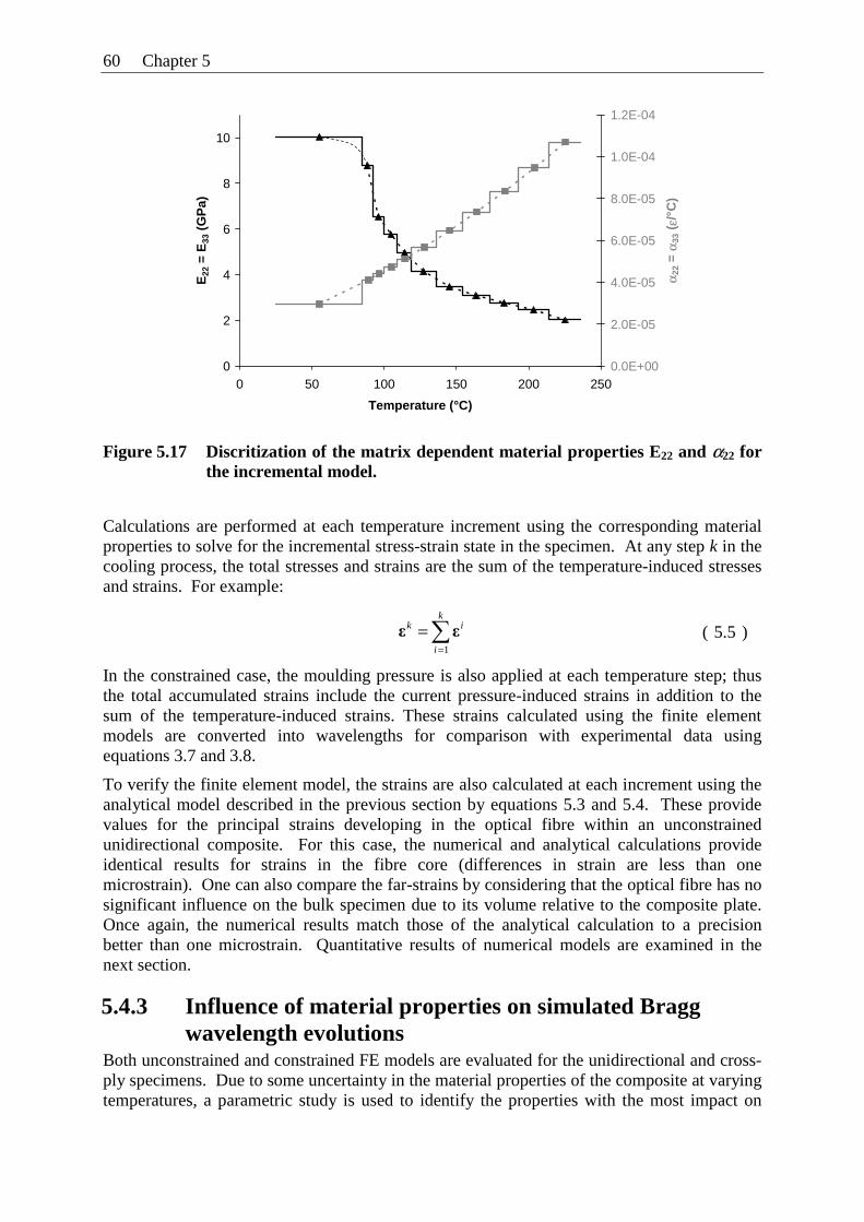
60 Chapter 5
0
2
4
6
8
10
0 50 100 150 200 250
Temperature (°C)
E22
= E
33 (
GP
a)
0.0E+00
2.0E-05
4.0E-05
6.0E-05
8.0E-05
1.0E-04
1.2E-04
α 22
= α 3
3 ( ε
/°C
)
Figure 5.17 Discritization of the matrix dependent material properties E22 and α22 for the incremental model.
Calculations are performed at each temperature increment using the corresponding material properties to solve for the incremental stress-strain state in the specimen. At any step k in the cooling process, the total stresses and strains are the sum of the temperature-induced stresses and strains. For example:
In the constrained case, the moulding pressure is also applied at each temperature step; thus the total accumulated strains include the current pressure-induced strains in addition to the sum of the temperature-induced strains. These strains calculated using the finite element models are converted into wavelengths for comparison with experimental data using equations 3.7 and 3.8.
To verify the finite element model, the strains are also calculated at each increment using the analytical model described in the previous section by equations 5.3 and 5.4. These provide values for the principal strains developing in the optical fibre within an unconstrained unidirectional composite. For this case, the numerical and analytical calculations provide identical results for strains in the fibre core (differences in strain are less than one microstrain). One can also compare the far-strains by considering that the optical fibre has no significant influence on the bulk specimen due to its volume relative to the composite plate. Once again, the numerical results match those of the analytical calculation to a precision better than one microstrain. Quantitative results of numerical models are examined in the next section.
5.4.3 Influence of material properties on simulated Bragg wavelength evolutions
Both unconstrained and constrained FE models are evaluated for the unidirectional and cross-ply specimens. Due to some uncertainty in the material properties of the composite at varying temperatures, a parametric study is used to identify the properties with the most impact on
∑=
=k
i
ik
1
εε ( 5.5 )
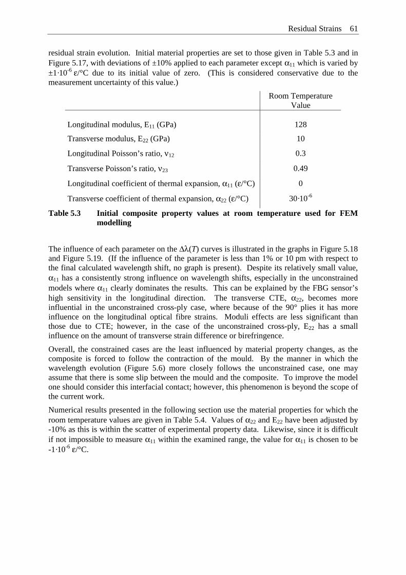
Residual Strains 61
residual strain evolution. Initial material properties are set to those given in Table 5.3 and in Figure 5.17, with deviations of ±10% applied to each parameter except α11 which is varied by ±1·10-6 ε/°C due to its initial value of zero. (This is considered conservative due to the measurement uncertainty of this value.)
Room Temperature
Value Longitudinal modulus, E11 (GPa)
128
Transverse modulus, E22 (GPa) 10
Longitudinal Poisson’s ratio, ν12 0.3
Transverse Poisson’s ratio, ν23 0.49
Longitudinal coefficient of thermal expansion, α11 (ε/°C) 0
Transverse coefficient of thermal expansion, α22 (ε/°C) 30·10-6
Table 5.3 Initial composite property values at room temperature used for FEM modelling
The influence of each parameter on the Δλ(T) curves is illustrated in the graphs in Figure 5.18 and Figure 5.19. (If the influence of the parameter is less than 1% or 10 pm with respect to the final calculated wavelength shift, no graph is present). Despite its relatively small value, α11 has a consistently strong influence on wavelength shifts, especially in the unconstrained models where α11 clearly dominates the results. This can be explained by the FBG sensor’s high sensitivity in the longitudinal direction. The transverse CTE, α22, becomes more influential in the unconstrained cross-ply case, where because of the 90° plies it has more influence on the longitudinal optical fibre strains. Moduli effects are less significant than those due to CTE; however, in the case of the unconstrained cross-ply, E22 has a small influence on the amount of transverse strain difference or birefringence.
Overall, the constrained cases are the least influenced by material property changes, as the composite is forced to follow the contraction of the mould. By the manner in which the wavelength evolution (Figure 5.6) more closely follows the unconstrained case, one may assume that there is some slip between the mould and the composite. To improve the model one should consider this interfacial contact; however, this phenomenon is beyond the scope of the current work.
Numerical results presented in the following section use the material properties for which the room temperature values are given in Table 5.4. Values of α22 and E22 have been adjusted by -10% as this is within the scatter of experimental property data. Likewise, since it is difficult if not impossible to measure α11 within the examined range, the value for α11 is chosen to be -1·10-6 ε/°C.
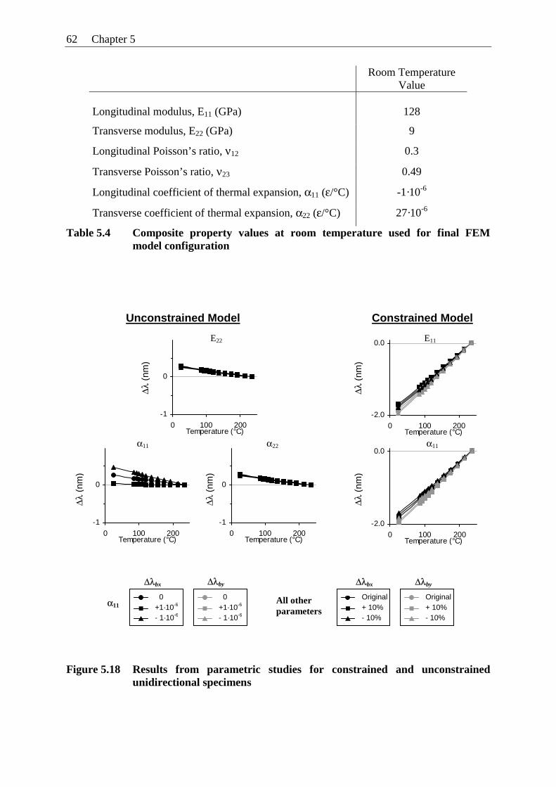
62 Chapter 5
Room Temperature
Value Longitudinal modulus, E11 (GPa)
128
Transverse modulus, E22 (GPa) 9
Longitudinal Poisson’s ratio, ν12 0.3
Transverse Poisson’s ratio, ν23 0.49
Longitudinal coefficient of thermal expansion, α11 (ε/°C) -1·10-6
Transverse coefficient of thermal expansion, α22 (ε/°C) 27·10-6
Table 5.4 Composite property values at room temperature used for final FEM model configuration
Figure 5.18 Results from parametric studies for constrained and unconstrained unidirectional specimens
-1
0
0 100 200Temperature (°C)
-1
0
0 100 200Temperature (°C)
-1
0
0 100 200Temperature (°C)
-2.0
0.0
0 100 200Temperature (°C)
-2.0
0.0
0 100 200Temperature (°C)
α22 α11
E22
α11
E11
Unconstrained Model Constrained Model
- 10% - 10%
α11 All other parameters
Original+ 10%
0+1·10-6
- 1·10-6
0+1·10-6
- 1·10-6
Original + 10%
Δλbx Δλby Δλby
Δλ (
nm)
Δλbx
Δλ (
nm)
Δλ (
nm)
Δλ (
nm)
Δλ (
nm)
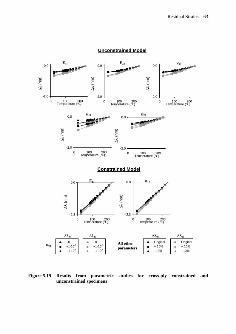
Residual Strains 63
Figure 5.19 Results from parametric studies for cross-ply constrained and unconstrained specimens
Unconstrained Model
-2.0
0.0
0 100 200Temperature (°C)
-2.0
0.0
0 100 200Temperature (°C)
-2.0
0.0
0 100 200Temperature (°C)
-2.0
0.0
0 100 200Temperature (°C)
-2.0
0.0
0 100 200Temperature (°C)
α22 α11
E22 E11 ν12
-2.3
0.0
0 100 200Temperature (°C)
E11
-2.3
0.0
0 100 200Temperature (°C)
α11
Constrained Model
- 10% - 10%
α11 All other parameters
Original + 10%
0+1·10-6 - 1·10-6
0+1·10-6
- 1·10-6
Original + 10%
Δλbx Δλby Δλbx Δλby
Δλ (
nm)
Δλ (
nm)
Δλ (
nm)
Δλ (
nm)
Δλ (
nm)
Δλ (
nm)
Δλ (
nm)
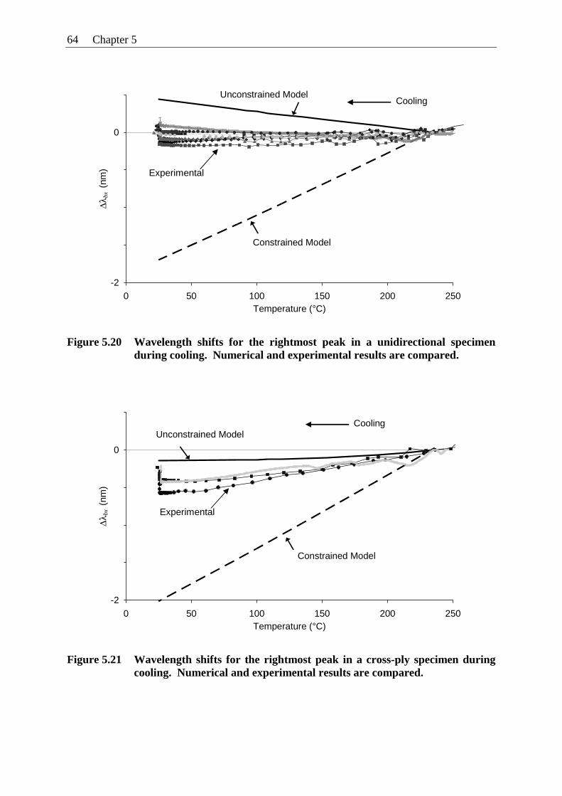
64 Chapter 5
Figure 5.20 Wavelength shifts for the rightmost peak in a unidirectional specimen during cooling. Numerical and experimental results are compared.
Figure 5.21 Wavelength shifts for the rightmost peak in a cross-ply specimen during cooling. Numerical and experimental results are compared.
-2
0
0 50 100 150 200 250Temperature (°C)
Δλbx
(nm
)Cooling
Constrained Model
Unconstrained Model
Experimental
-2
0
0 50 100 150 200 250Temperature (°C)
Δλbx
(nm
)
Cooling
Constrained Model
Unconstrained Model
Experimental
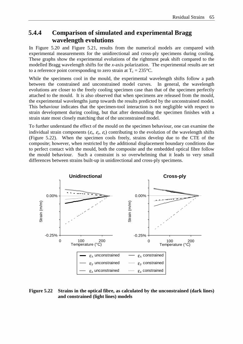
Residual Strains 65
5.4.4 Comparison of simulated and experimental Bragg wavelength evolutions
In Figure 5.20 and Figure 5.21, results from the numerical models are compared with experimental measurements for the unidirectional and cross-ply specimens during cooling. These graphs show the experimental evolutions of the rightmost peak shift compared to the modelled Bragg wavelength shifts for the x-axis polarization. The experimental results are set to a reference point corresponding to zero strain at Tc = 235°C.
While the specimens cool in the mould, the experimental wavelength shifts follow a path between the constrained and unconstrained model curves. In general, the wavelength evolutions are closer to the freely cooling specimen case than that of the specimen perfectly attached to the mould. It is also observed that when specimens are released from the mould, the experimental wavelengths jump towards the results predicted by the unconstrained model. This behaviour indicates that the specimen-tool interaction is not negligible with respect to strain development during cooling, but that after demoulding the specimen finishes with a strain state most closely matching that of the unconstrained model.
To further understand the effect of the mould on the specimen behaviour, one can examine the individual strain components (εx, εy, εz) contributing to the evolution of the wavelength shifts (Figure 5.22). When the specimen cools freely, strains develop due to the CTE of the composite; however, when restricted by the additional displacement boundary conditions due to perfect contact with the mould, both the composite and the embedded optical fibre follow the mould behaviour. Such a constraint is so overwhelming that it leads to very small differences between strains built-up in unidirectional and cross-ply specimens.
Figure 5.22 Strains in the optical fibre, as calculated by the unconstrained (dark lines) and constrained (light lines) models
-0.25%
0.00%
0 100 200Temperature (°C)
Str
ain
(m/m
)
-0.25%
0.00%
0 100 200Temperature (°C)
Str
ain
(m/m
)
εx constrained
εy constrained
εz constrained
εx unconstrained
εy unconstrained
εz unconstrained
Unidirectional Cross-ply
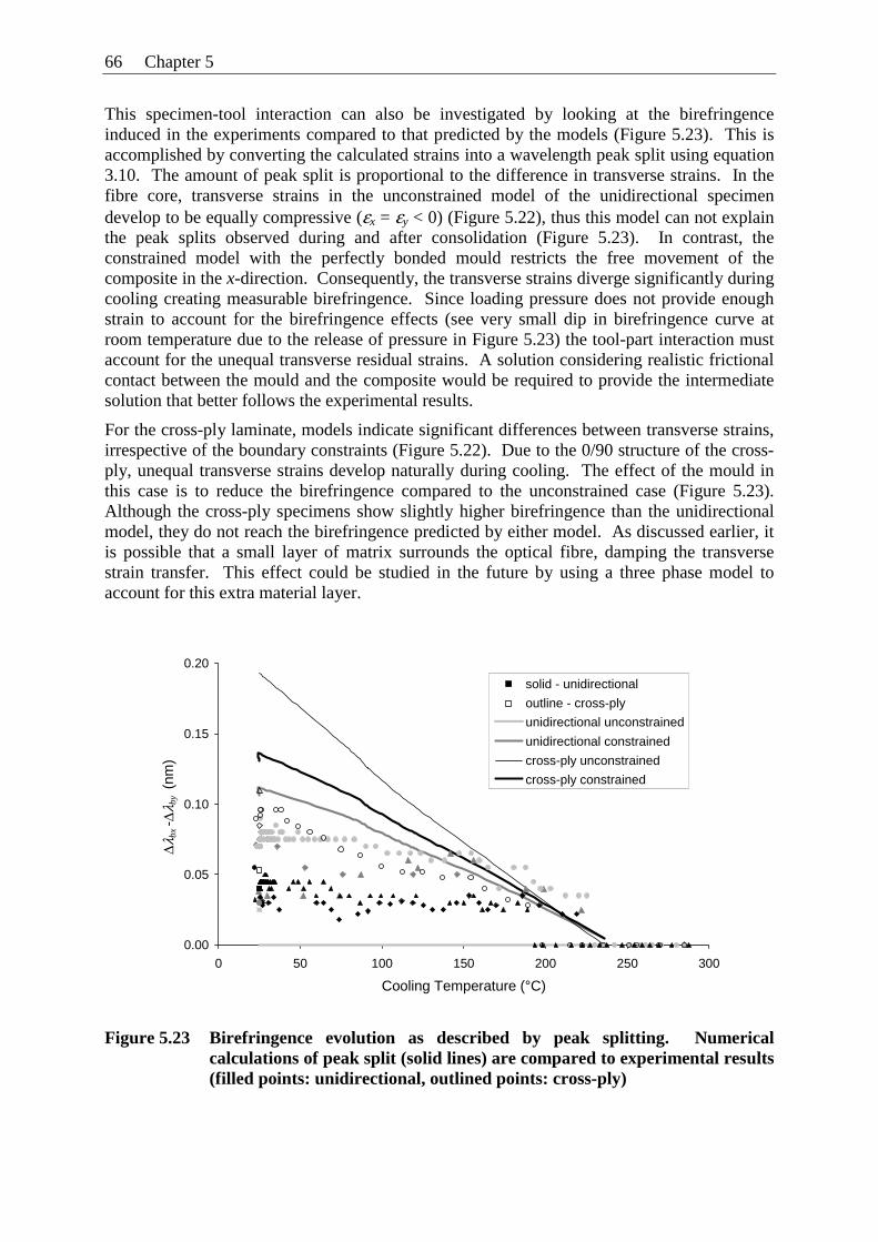
66 Chapter 5
This specimen-tool interaction can also be investigated by looking at the birefringence induced in the experiments compared to that predicted by the models (Figure 5.23). This is accomplished by converting the calculated strains into a wavelength peak split using equation 3.10. The amount of peak split is proportional to the difference in transverse strains. In the fibre core, transverse strains in the unconstrained model of the unidirectional specimen develop to be equally compressive (εx = εy < 0) (Figure 5.22), thus this model can not explain the peak splits observed during and after consolidation (Figure 5.23). In contrast, the constrained model with the perfectly bonded mould restricts the free movement of the composite in the x-direction. Consequently, the transverse strains diverge significantly during cooling creating measurable birefringence. Since loading pressure does not provide enough strain to account for the birefringence effects (see very small dip in birefringence curve at room temperature due to the release of pressure in Figure 5.23) the tool-part interaction must account for the unequal transverse residual strains. A solution considering realistic frictional contact between the mould and the composite would be required to provide the intermediate solution that better follows the experimental results.
For the cross-ply laminate, models indicate significant differences between transverse strains, irrespective of the boundary constraints (Figure 5.22). Due to the 0/90 structure of the cross-ply, unequal transverse strains develop naturally during cooling. The effect of the mould in this case is to reduce the birefringence compared to the unconstrained case (Figure 5.23). Although the cross-ply specimens show slightly higher birefringence than the unidirectional model, they do not reach the birefringence predicted by either model. As discussed earlier, it is possible that a small layer of matrix surrounds the optical fibre, damping the transverse strain transfer. This effect could be studied in the future by using a three phase model to account for this extra material layer.
0.00
0.05
0.10
0.15
0.20
0 50 100 150 200 250 300
Cooling Temperature (°C)
Δλbx
- Δλ b
y (
nm)
solid - unidirectional
outline - cross-ply
unidirectional unconstrained
unidirectional constrained
cross-ply unconstrained
cross-ply constrained
Figure 5.23 Birefringence evolution as described by peak splitting. Numerical calculations of peak split (solid lines) are compared to experimental results (filled points: unidirectional, outlined points: cross-ply)
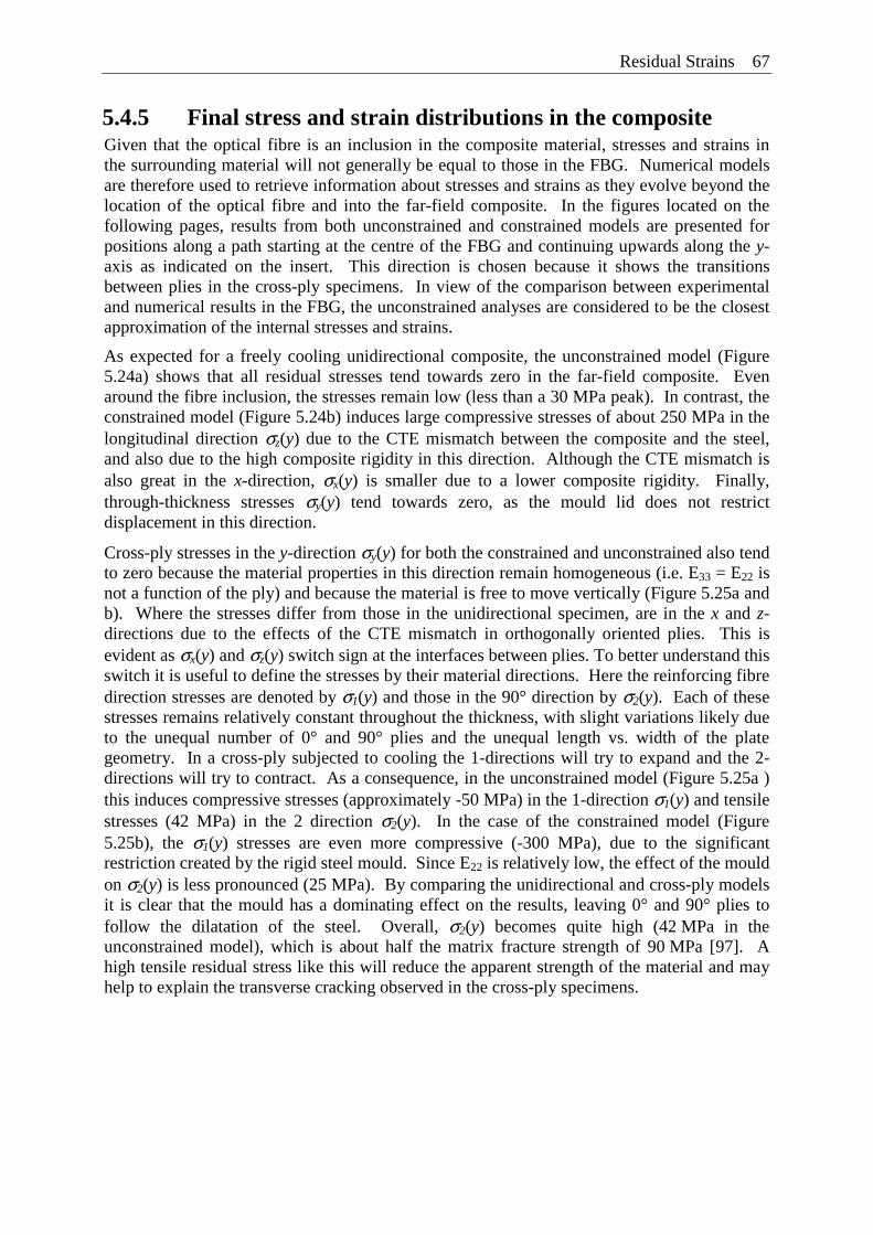
Residual Strains 67
5.4.5 Final stress and strain distributions in the composite Given that the optical fibre is an inclusion in the composite material, stresses and strains in the surrounding material will not generally be equal to those in the FBG. Numerical models are therefore used to retrieve information about stresses and strains as they evolve beyond the location of the optical fibre and into the far-field composite. In the figures located on the following pages, results from both unconstrained and constrained models are presented for positions along a path starting at the centre of the FBG and continuing upwards along the y-axis as indicated on the insert. This direction is chosen because it shows the transitions between plies in the cross-ply specimens. In view of the comparison between experimental and numerical results in the FBG, the unconstrained analyses are considered to be the closest approximation of the internal stresses and strains.
As expected for a freely cooling unidirectional composite, the unconstrained model (Figure 5.24a) shows that all residual stresses tend towards zero in the far-field composite. Even around the fibre inclusion, the stresses remain low (less than a 30 MPa peak). In contrast, the constrained model (Figure 5.24b) induces large compressive stresses of about 250 MPa in the longitudinal direction σz(y) due to the CTE mismatch between the composite and the steel, and also due to the high composite rigidity in this direction. Although the CTE mismatch is also great in the x-direction, σx(y) is smaller due to a lower composite rigidity. Finally, through-thickness stresses σy(y) tend towards zero, as the mould lid does not restrict displacement in this direction.
Cross-ply stresses in the y-direction σy(y) for both the constrained and unconstrained also tend to zero because the material properties in this direction remain homogeneous (i.e. E33 = E22 is not a function of the ply) and because the material is free to move vertically (Figure 5.25a and b). Where the stresses differ from those in the unidirectional specimen, are in the x and z-directions due to the effects of the CTE mismatch in orthogonally oriented plies. This is evident as σx(y) and σz(y) switch sign at the interfaces between plies. To better understand this switch it is useful to define the stresses by their material directions. Here the reinforcing fibre direction stresses are denoted by σ1(y) and those in the 90° direction by σ2(y). Each of these stresses remains relatively constant throughout the thickness, with slight variations likely due to the unequal number of 0° and 90° plies and the unequal length vs. width of the plate geometry. In a cross-ply subjected to cooling the 1-directions will try to expand and the 2-directions will try to contract. As a consequence, in the unconstrained model (Figure 5.25a ) this induces compressive stresses (approximately -50 MPa) in the 1-direction σ1(y) and tensile stresses (42 MPa) in the 2 direction σ2(y). In the case of the constrained model (Figure 5.25b), the σ1(y) stresses are even more compressive (-300 MPa), due to the significant restriction created by the rigid steel mould. Since E22 is relatively low, the effect of the mould on σ2(y) is less pronounced (25 MPa). By comparing the unidirectional and cross-ply models it is clear that the mould has a dominating effect on the results, leaving 0° and 90° plies to follow the dilatation of the steel. Overall, σ2(y) becomes quite high (42 MPa in the unconstrained model), which is about half the matrix fracture strength of 90 MPa [97]. A high tensile residual stress like this will reduce the apparent strength of the material and may help to explain the transverse cracking observed in the cross-ply specimens.
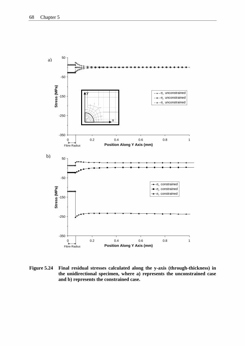
68 Chapter 5
-350
-250
-150
-50
50
0 0.2 0.4 0.6 0.8 1
Position Along Y Axis (mm)
Str
ess
(MP
a)
s1s2s3
Fibre Radius
σx unconstrainedσy unconstrainedσz unconstrained
-350
-250
-150
-50
50
0 0.2 0.4 0.6 0.8 1
Position Along Y Axis (mm)
Str
ess
(MP
a)
s1s2s3
Fibre Radius
σx constrainedσy constrainedσz constrained
Figure 5.24 Final residual stresses calculated along the y-axis (through-thickness) in the unidirectional specimen, where a) represents the unconstrained case and b) represents the constrained case.
a)
b)
y
x
Residual Strains 69
Figure 5.25 Final residual stresses calculated along the y-axis (through-thickness) in the cross-ply specimen, where a) represents the unconstrained case and b) represents the constrained case.
-350
-250
-150
-50
50
0 0.2 0.4 0.6 0.8 1
Position Along Y Axis (mm)
Str
ess
(MP
a)
s1s2s3
Fibre Radius
σx unconstrainedσy unconstrainedσz unconstrained
y
x
0° ply
-350
-250
-150
-50
50
0 0.2 0.4 0.6 0.8 1
Position Along Y Axis (mm)
Str
ess
(MP
a)
s1s2s3
Fibre Radius
σx constrainedσy constrainedσz constrained
a)
b)
90° ply 0° ply
σ2(y)
σ1(y)
σ3(y)
0° ply 90° ply 0° ply
σ2(y)
σ1(y)
σ3(y)
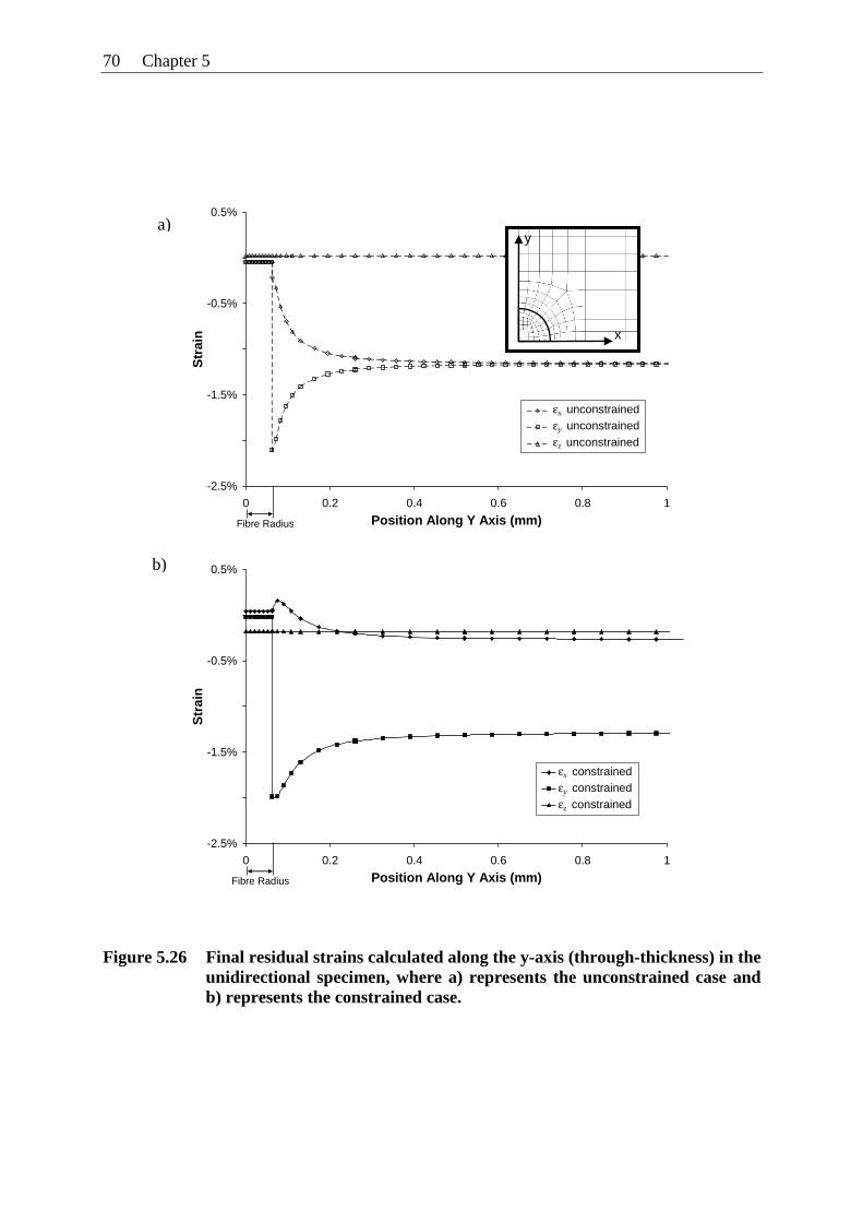
70 Chapter 5
-2.5%
-1.5%
-0.5%
0.5%
0 0.2 0.4 0.6 0.8 1
Position Along Y Axis (mm)
Str
ain
e1e2e3
Fibre Radius
εx unconstrainedεy unconstrainedεz unconstrained
-2.5%
-1.5%
-0.5%
0.5%
0 0.2 0.4 0.6 0.8 1
Position Along Y Axis (mm)
Str
ain
e1e2e3
Fibre Radius
εx constrainedεy constrainedεz constrained
Figure 5.26 Final residual strains calculated along the y-axis (through-thickness) in the unidirectional specimen, where a) represents the unconstrained case and b) represents the constrained case.
a)
b)
y
x
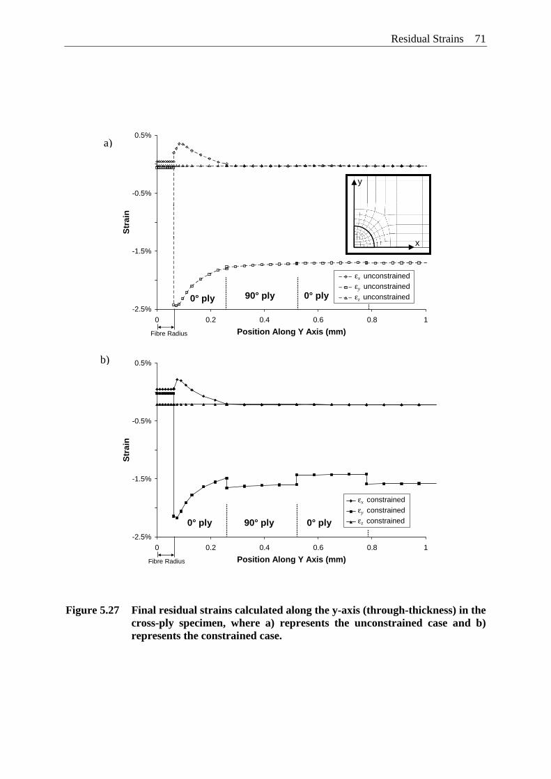
Residual Strains 71
-2.5%
-1.5%
-0.5%
0.5%
0 0.2 0.4 0.6 0.8 1
Position Along Y Axis (mm)
Str
ain
e1e2e3
Fibre Radius
εx unconstrainedεy unconstrainedεz unconstrained
-2.5%
-1.5%
-0.5%
0.5%
0 0.2 0.4 0.6 0.8 1
Position Along Y Axis (mm)
Str
ain
e1e2e3
Fibre Radius
εx constrainedεy constrainedεz constrained
Figure 5.27 Final residual strains calculated along the y-axis (through-thickness) in the cross-ply specimen, where a) represents the unconstrained case and b) represents the constrained case.
a)
b)
y
x
0° ply 90° ply 0° ply
0° ply 90° ply 0° ply
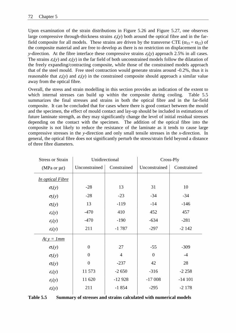
72 Chapter 5
Upon examination of the strain distributions in Figure 5.26 and Figure 5.27, one observes large compressive through-thickness strains εy(y) both around the optical fibre and in the far-field composite for all models. These strains are driven by the transverse CTE (α33 = α22) of the composite material and are free to develop as there is no restriction on displacement in the y-direction. At the fibre interface these compressive strains εy(y) approach 2.5% in all cases. The strains εx(y) and εz(y) in the far field of both unconstrained models follow the dilatation of the freely expanding/contracting composite, while those of the constrained models approach that of the steel mould. Free steel contraction would generate strains around -0.2%, thus it is reasonable that εx(y) and εz(y) in the constrained composite should approach a similar value away from the optical fibre.
Overall, the stress and strain modelling in this section provides an indication of the extent to which internal stresses can build up within the composite during cooling. Table 5.5 summarizes the final stresses and strains in both the optical fibre and in the far-field composite. It can be concluded that for cases where there is good contact between the mould and the specimen, the effect of mould contact and lay-up should be included in estimations of future laminate strength, as they may significantly change the level of initial residual stresses depending on the contact with the specimen. The addition of the optical fibre into the composite is not likely to reduce the resistance of the laminate as it tends to cause large compressive stresses in the y-direction and only small tensile stresses in the x-direction. In general, the optical fibre does not significantly perturb the stress/strain field beyond a distance of three fibre diameters.
Stress or Strain Unidirectional Cross-Ply
(MPa or με) Unconstrained Constrained Unconstrained Constrained
In optical Fibre
σx(y) -28 13 31 10
σy(y) -28 -23 -34 -34
σz(y) 13 -119 -14 -146
εx(y) -470 410 452 457
εy(y) -470 -190 -634 -281
εz(y) 211 -1 787 -297 -2 142
At y = 1mm
σx(y) 0 27 -55 -309
σy(y) 0 4 0 -4
σz(y) 0 -237 42 28
εx(y) 11 573 -2 650 -316 -2 258
εy(y) 11 620 -12 928 -17 008 -14 101
εz(y) 211 -1 854 -295 -2 178
Table 5.5 Summary of stresses and strains calculated with numerical models
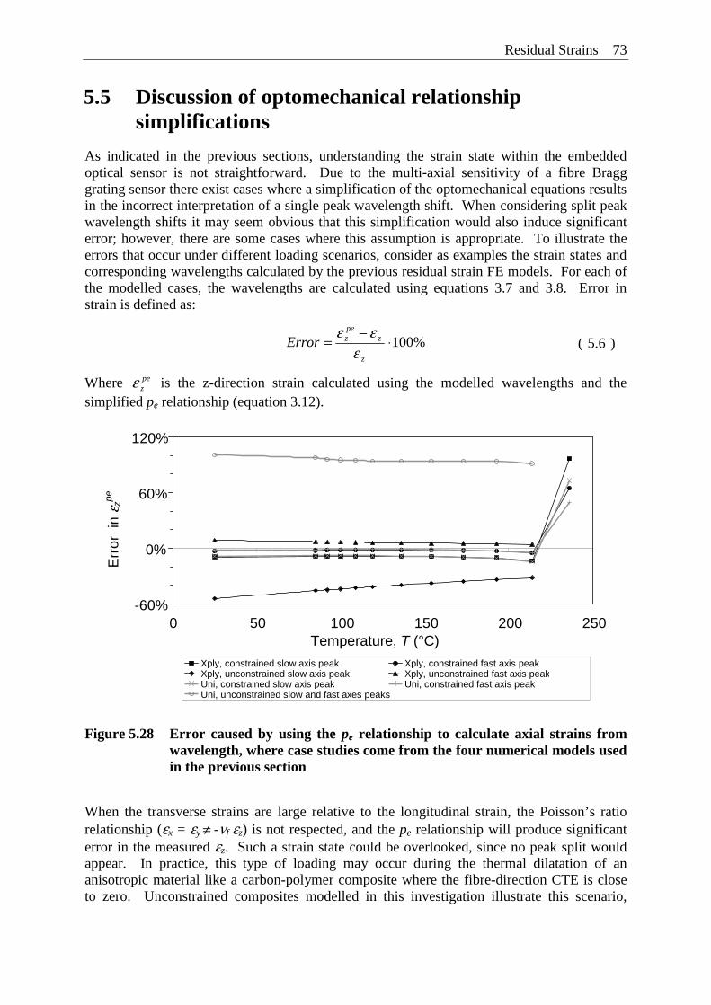
Residual Strains 73
5.5 Discussion of optomechanical relationship simplifications
As indicated in the previous sections, understanding the strain state within the embedded optical sensor is not straightforward. Due to the multi-axial sensitivity of a fibre Bragg grating sensor there exist cases where a simplification of the optomechanical equations results in the incorrect interpretation of a single peak wavelength shift. When considering split peak wavelength shifts it may seem obvious that this simplification would also induce significant error; however, there are some cases where this assumption is appropriate. To illustrate the errors that occur under different loading scenarios, consider as examples the strain states and corresponding wavelengths calculated by the previous residual strain FE models. For each of the modelled cases, the wavelengths are calculated using equations 3.7 and 3.8. Error in strain is defined as:
Where pezε is the z-direction strain calculated using the modelled wavelengths and the
simplified pe relationship (equation 3.12).
Figure 5.28 Error caused by using the pe relationship to calculate axial strains from wavelength, where case studies come from the four numerical models used in the previous section
When the transverse strains are large relative to the longitudinal strain, the Poisson’s ratio relationship (εx = εy ≠ -νf εz) is not respected, and the pe relationship will produce significant error in the measured εz. Such a strain state could be overlooked, since no peak split would appear. In practice, this type of loading may occur during the thermal dilatation of an anisotropic material like a carbon-polymer composite where the fibre-direction CTE is close to zero. Unconstrained composites modelled in this investigation illustrate this scenario,
%100⋅−
=z
zpezError
εεε
( 5.6 )
-60%
0%
60%
120%
0 50 100 150 200 250Temperature, T (°C)
Err
or i
n ε z
pe
Xply, constrained slow axis peak Xply, constrained fast axis peakXply, unconstrained slow axis peak Xply, unconstrained fast axis peak Uni, constrained slow axis peak Uni, constrained fast axis peakUni, unconstrained slow and fast axes peaks
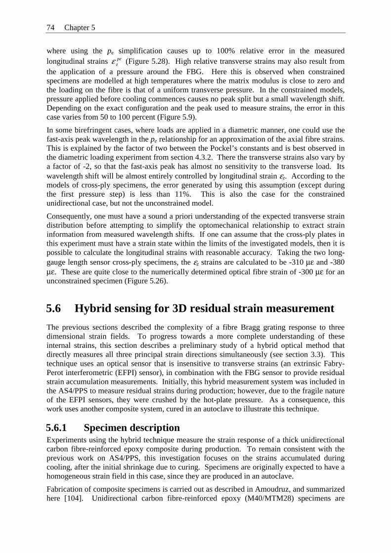
74 Chapter 5
where using the pe simplification causes up to 100% relative error in the measured longitudinal strains pe
zε (Figure 5.28). High relative transverse strains may also result from the application of a pressure around the FBG. Here this is observed when constrained specimens are modelled at high temperatures where the matrix modulus is close to zero and the loading on the fibre is that of a uniform transverse pressure. In the constrained models, pressure applied before cooling commences causes no peak split but a small wavelength shift. Depending on the exact configuration and the peak used to measure strains, the error in this case varies from 50 to 100 percent (Figure 5.9).
In some birefringent cases, where loads are applied in a diametric manner, one could use the fast-axis peak wavelength in the pe relationship for an approximation of the axial fibre strains. This is explained by the factor of two between the Pockel’s constants and is best observed in the diametric loading experiment from section 4.3.2. There the transverse strains also vary by a factor of -2, so that the fast-axis peak has almost no sensitivity to the transverse load. Its wavelength shift will be almost entirely controlled by longitudinal strain εz. According to the models of cross-ply specimens, the error generated by using this assumption (except during the first pressure step) is less than 11%. This is also the case for the constrained unidirectional case, but not the unconstrained model.
Consequently, one must have a sound a priori understanding of the expected transverse strain distribution before attempting to simplify the optomechanical relationship to extract strain information from measured wavelength shifts. If one can assume that the cross-ply plates in this experiment must have a strain state within the limits of the investigated models, then it is possible to calculate the longitudinal strains with reasonable accuracy. Taking the two long-gauge length sensor cross-ply specimens, the εz strains are calculated to be -310 με and -380 με. These are quite close to the numerically determined optical fibre strain of -300 με for an unconstrained specimen (Figure 5.26).
5.6 Hybrid sensing for 3D residual strain measurement
The previous sections described the complexity of a fibre Bragg grating response to three dimensional strain fields. To progress towards a more complete understanding of these internal strains, this section describes a preliminary study of a hybrid optical method that directly measures all three principal strain directions simultaneously (see section 3.3). This technique uses an optical sensor that is insensitive to transverse strains (an extrinsic Fabry-Perot interferometric (EFPI) sensor), in combination with the FBG sensor to provide residual strain accumulation measurements. Initially, this hybrid measurement system was included in the AS4/PPS to measure residual strains during production; however, due to the fragile nature of the EFPI sensors, they were crushed by the hot-plate pressure. As a consequence, this work uses another composite system, cured in an autoclave to illustrate this technique.
5.6.1 Specimen description Experiments using the hybrid technique measure the strain response of a thick unidirectional carbon fibre-reinforced epoxy composite during production. To remain consistent with the previous work on AS4/PPS, this investigation focuses on the strains accumulated during cooling, after the initial shrinkage due to curing. Specimens are originally expected to have a homogeneous strain field in this case, since they are produced in an autoclave.
Fabrication of composite specimens is carried out as described in Amoudruz, and summarized here [104]. Unidirectional carbon fibre-reinforced epoxy (M40/MTM28) specimens are
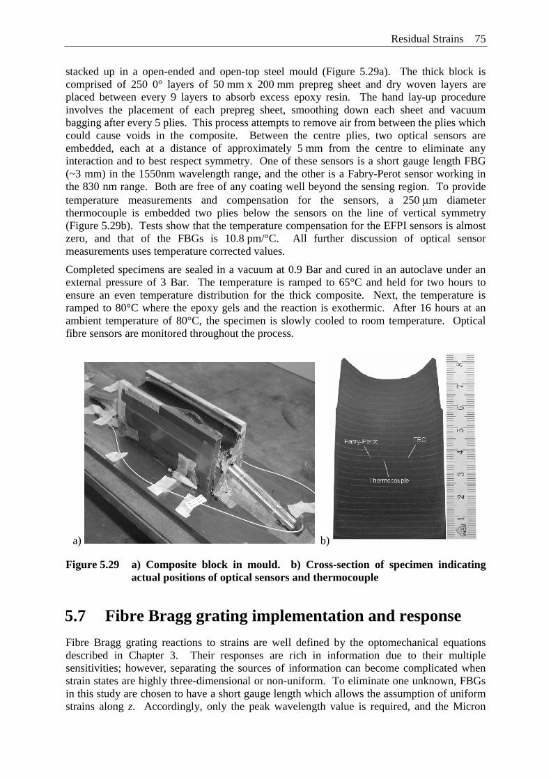
Residual Strains 75
stacked up in a open-ended and open-top steel mould (Figure 5.29a). The thick block is comprised of 250 0° layers of 50 mm x 200 mm prepreg sheet and dry woven layers are placed between every 9 layers to absorb excess epoxy resin. The hand lay-up procedure involves the placement of each prepreg sheet, smoothing down each sheet and vacuum bagging after every 5 plies. This process attempts to remove air from between the plies which could cause voids in the composite. Between the centre plies, two optical sensors are embedded, each at a distance of approximately 5 mm from the centre to eliminate any interaction and to best respect symmetry. One of these sensors is a short gauge length FBG (~3 mm) in the 1550nm wavelength range, and the other is a Fabry-Perot sensor working in the 830 nm range. Both are free of any coating well beyond the sensing region. To provide temperature measurements and compensation for the sensors, a 250 μm diameter thermocouple is embedded two plies below the sensors on the line of vertical symmetry (Figure 5.29b). Tests show that the temperature compensation for the EFPI sensors is almost zero, and that of the FBGs is 10.8 pm/°C. All further discussion of optical sensor measurements uses temperature corrected values.
Completed specimens are sealed in a vacuum at 0.9 Bar and cured in an autoclave under an external pressure of 3 Bar. The temperature is ramped to 65°C and held for two hours to ensure an even temperature distribution for the thick composite. Next, the temperature is ramped to 80°C where the epoxy gels and the reaction is exothermic. After 16 hours at an ambient temperature of 80°C, the specimen is slowly cooled to room temperature. Optical fibre sensors are monitored throughout the process.
a) b)
Figure 5.29 a) Composite block in mould. b) Cross-section of specimen indicating actual positions of optical sensors and thermocouple
5.7 Fibre Bragg grating implementation and response
Fibre Bragg grating reactions to strains are well defined by the optomechanical equations described in Chapter 3. Their responses are rich in information due to their multiple sensitivities; however, separating the sources of information can become complicated when strain states are highly three-dimensional or non-uniform. To eliminate one unknown, FBGs in this study are chosen to have a short gauge length which allows the assumption of uniform strains along z. Accordingly, only the peak wavelength value is required, and the Micron
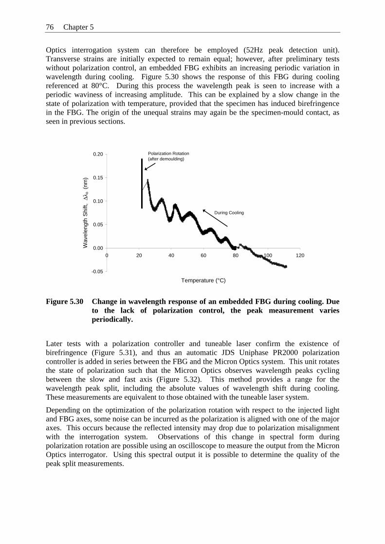
76 Chapter 5
Optics interrogation system can therefore be employed (52Hz peak detection unit). Transverse strains are initially expected to remain equal; however, after preliminary tests without polarization control, an embedded FBG exhibits an increasing periodic variation in wavelength during cooling. Figure 5.30 shows the response of this FBG during cooling referenced at 80°C. During this process the wavelength peak is seen to increase with a periodic waviness of increasing amplitude. This can be explained by a slow change in the state of polarization with temperature, provided that the specimen has induced birefringence in the FBG. The origin of the unequal strains may again be the specimen-mould contact, as seen in previous sections.
-0.05
0.00
0.05
0.10
0.15
0.20
0 20 40 60 80 100 120
Temperature (°C)
Wav
elen
gth
Shi
ft, Δ
λ b (
nm)
Polarization Rotation(after demoulding)
During Cooling
Figure 5.30 Change in wavelength response of an embedded FBG during cooling. Due to the lack of polarization control, the peak measurement varies periodically.
Later tests with a polarization controller and tuneable laser confirm the existence of birefringence (Figure 5.31), and thus an automatic JDS Uniphase PR2000 polarization controller is added in series between the FBG and the Micron Optics system. This unit rotates the state of polarization such that the Micron Optics observes wavelength peaks cycling between the slow and fast axis (Figure 5.32). This method provides a range for the wavelength peak split, including the absolute values of wavelength shift during cooling. These measurements are equivalent to those obtained with the tuneable laser system.
Depending on the optimization of the polarization rotation with respect to the injected light and FBG axes, some noise can be incurred as the polarization is aligned with one of the major axes. This occurs because the reflected intensity may drop due to polarization misalignment with the interrogation system. Observations of this change in spectral form during polarization rotation are possible using an oscilloscope to measure the output from the Micron Optics interrogator. Using this spectral output it is possible to determine the quality of the peak split measurements.
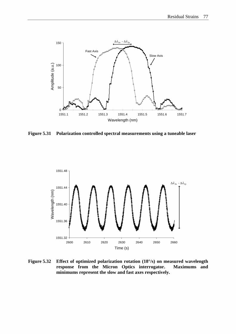
Residual Strains 77
0
50
100
150
1551.1 1551.2 1551.3 1551.4 1551.5 1551.6 1551.7
Wavelength (nm)
Am
plitu
de (
a.u.
)Slow Axis
Fast Axis
Δλ bx - Δλ by
Figure 5.31 Polarization controlled spectral measurements using a tuneable laser
1551.32
1551.36
1551.40
1551.44
1551.48
2600 2610 2620 2630 2640 2650 2660
Time (s)
Wav
elen
gth
(nm
)
Δλ bx - Δλ by
Figure 5.32 Effect of optimized polarization rotation (18°/s) on measured wavelength response from the Micron Optics interrogator. Maximums and minimums represent the slow and fast axes respectively.
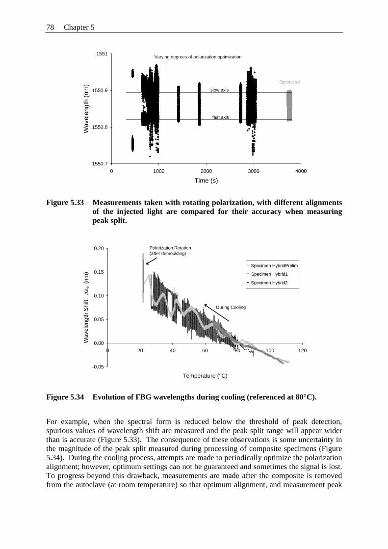
78 Chapter 5
1550.7
1550.8
1550.9
1551
0 1000 2000 3000 4000
Time (s)
Wav
elen
gth
(nm
)
Varying degrees of polarization optimization
Optimized
slow axis
fast axis
Figure 5.33 Measurements taken with rotating polarization, with different alignments of the injected light are compared for their accuracy when measuring peak split.
-0.05
0.00
0.05
0.10
0.15
0.20
0 20 40 60 80 100 120
Temperature (°C)
Wav
elen
gth
Shi
ft, Δ
λ b (
nm)
Polarization Rotation(after demoulding)
During Cooling
- Specimen HybridPrelim
- Specimen Hybrid1
- Specimen Hybrid2
Figure 5.34 Evolution of FBG wavelengths during cooling (referenced at 80°C).
For example, when the spectral form is reduced below the threshold of peak detection, spurious values of wavelength shift are measured and the peak split range will appear wider than is accurate (Figure 5.33). The consequence of these observations is some uncertainty in the magnitude of the peak split measured during processing of composite specimens (Figure 5.34). During the cooling process, attempts are made to periodically optimize the polarization alignment; however, optimum settings can not be guaranteed and sometimes the signal is lost. To progress beyond this drawback, measurements are made after the composite is removed from the autoclave (at room temperature) so that optimum alignment, and measurement peak
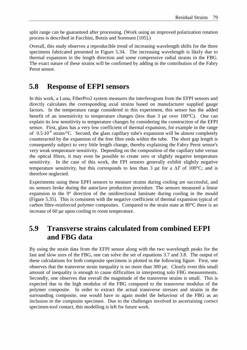
Residual Strains 79
split range can be guaranteed after processing. (Work using an improved polarization rotation process is described in Facchini, Botsis and Sorensen [105].)
Overall, this study observes a reproducible trend of increasing wavelength shifts for the three specimens fabricated presented in Figure 5.34. The increasing wavelength is likely due to thermal expansion in the length direction and some compressive radial strains in the FBG. The exact nature of these strains will be confirmed by adding in the contribution of the Fabry Perot sensor.
5.8 Response of EFPI sensors
In this work, a Luna, FiberPro2 system measures the interferogram from the EFPI sensors and directly calculates the corresponding axial strains based on manufacturer supplied gauge factors. In the temperature range considered in this experiment, this sensor has the added benefit of an insensitivity to temperature changes (less than 3 με over 100°C). One can explain its low sensitivity to temperature changes by considering the construction of the EFPI sensor. First, glass has a very low coefficient of thermal expansion, for example in the range of 0.5·10-6 strain/°C. Second, the glass capillary tube's expansion will be almost completely counteracted by the expansion of the free fibre ends within the tube. The short gap length is consequently subject to very little length change, thereby explaining the Fabry Perot sensor's very weak temperature sensitivity. Depending on the composition of the capillary tube versus the optical fibres, it may even be possible to create zero or slightly negative temperature sensitivity. In the case of this work, the FPI sensors generally exhibit slightly negative temperature sensitivity, but this corresponds to less than 3 με for a ΔT of 100°C; and is therefore neglected.
Experiments using these EPFI sensors to measure strains during cooling are successful, and no sensors broke during the autoclave production procedure. The sensors measured a linear expansion in the 0° direction of the unidirectional laminate during cooling in the mould (Figure 5.35). This is consistent with the negative coefficient of thermal expansion typical of carbon fibre-reinforced polymer composites. Compared to the strain state at 80°C there is an increase of 60 με upon cooling to room temperature.
5.9 Transverse strains calculated from combined EFPI and FBG data
By using the strain data from the EFPI sensor along with the two wavelength peaks for the fast and slow axes of the FBG, one can solve the set of equations 3.7 and 3.8. The output of these calculations for both composite specimens is plotted in the following figure. First, one observes that the transverse strain inequality is no more than 300 με. Clearly even this small amount of inequality is enough to cause difficulties in interpreting solo FBG measurements. Secondly, one observes that overall the magnitude of the transverse strains is small. This is expected due to the high modulus of the FBG compared to the transverse modulus of the polymer composite. In order to extract the actual transverse stresses and strains in the surrounding composite, one would have to again model the behaviour of the FBG as an inclusion in the composite specimen. Due to the challenges involved in ascertaining correct specimen-tool contact, this modelling is left for future work.
80 Chapter 5
Figure 5.35 Increase in longitudinal strain measured by EFPI sensors during cooling
Figure 5.36 Evolution of transverse strains during cooling determined using EFPI and FBG data.
-300
-250
-200
-150
-100
-50
0
50
100
0 10 20 30 40 50 60 70 80 90
Temperature (°C)
Tra
nsve
rse
Str
ains
, (μm
/m)
slow axis
fast axis
During Cooling Specimen Hybrid1 Specimen Hybrid2
-40
-20
0
20
40
60
80
0 20 40 60 80 100 120
Temperature (°C)
Mic
rost
rain
, εz (μ
m/m
)
During Cooling
- Specimen Hybrid1
- Specimen Hybrid2
Long
itudi
nal S
trai
n, ε
z (μ
m/m
)
Chapter 6 Delamination
Fibre Bragg grating sensors are ideally suited to the continuous monitoring of structures: from processing to failure. The same sensor that measures process-induced strains may also provide information about material degradation and damage during the life of the structure. This chapter discusses the implementation of Mode I delamination tests with embedded FBG sensors for the purpose of measuring non-uniform strains during delamination cracking. It is shown that a specimen’s initial residual strain state in the sensor is not modified by cracking and can therefore be used as an initial point of reference. The initial state of birefringence does, however, require polarization adapted measurement techniques.
Experimental measurements and observations indicate that this type of delamination specimen incurs fibre bridging across the delamination plane. By combining the distribution of strains read by the FBG sensor with a numerical model, it is possible to determine the exact distribution of bridging stresses caused by these fibres. Results from this inverse numerical identification technique are then compared to the output from cohesive element modelling of the delamination cracking process.
6.1 Experimental – DCB testing
This section describes the preparation of specimens and the mechanical testing set-up. It also provides results that are traditionally obtained during double cantilever beam (DCB) experiments. These include the load-displacement behaviour and the energy release-rate (GI or R-curves) which give a macroscopic view of the specimen behaviour and test repeatability. They also include visual observations of crack growth and fibre bridging phenomena.
6.1.1 Specimen preparation Delamination specimen preparation follows the same basic production procedure used for all AS4/PPS specimens, with two additional requirements. First, a 60-70 mm long piece of aluminium foil treated with demoulding agent is inserted between the centre plies at one end of the specimen to create a pre-crack. The thermocouple is placed in the same layer. Second, the fibre optic sensor (FBG length 20-35 mm) is placed between the second and third layers above the centerline, parallel to the reinforcing fibres. Once consolidated, the axis of the FBG is located approximately two diameters (two ply widths or 0.264 mm) from the delamination plane. This distance is sufficiently removed from the crack to keep it from being damaged, while at the same time remaining close enough to guarantee the sensitivity of the sensor. The central location (along the length) also ensures that the pre-crack has no influence on the initial residual strains in the sensor. It was shown in Chapter 5 that the residual strain development measured by the FBG sensors in plates prepared with aluminium foil pre-cracks is comparable to that developed in the basic composite plates.
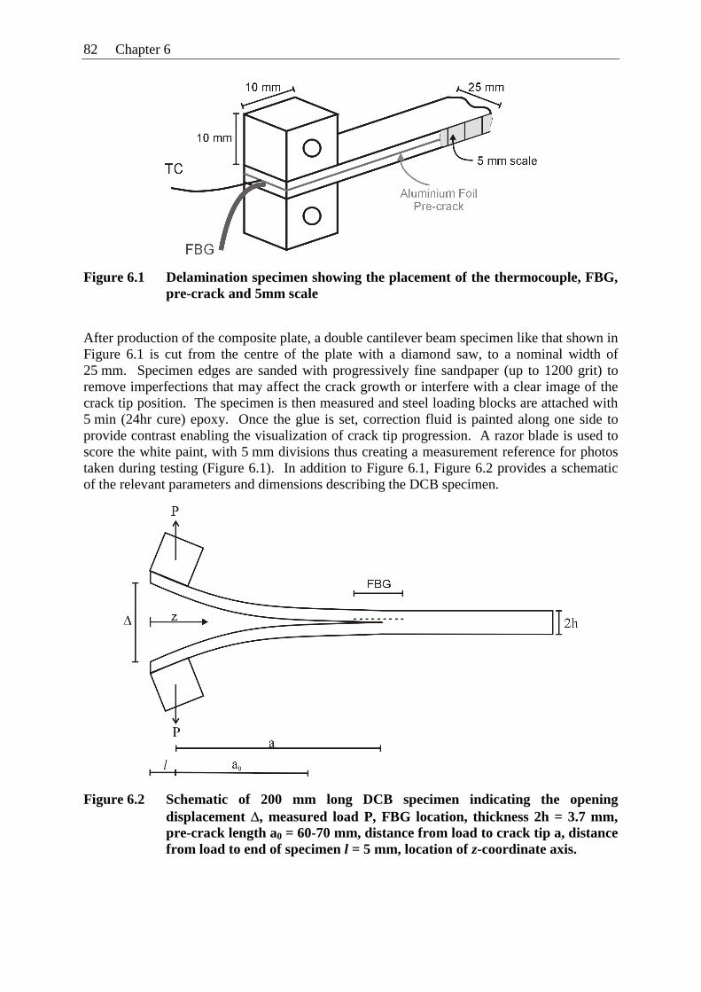
82 Chapter 6
Figure 6.1 Delamination specimen showing the placement of the thermocouple, FBG, pre-crack and 5mm scale
After production of the composite plate, a double cantilever beam specimen like that shown in Figure 6.1 is cut from the centre of the plate with a diamond saw, to a nominal width of 25 mm. Specimen edges are sanded with progressively fine sandpaper (up to 1200 grit) to remove imperfections that may affect the crack growth or interfere with a clear image of the crack tip position. The specimen is then measured and steel loading blocks are attached with 5 min (24hr cure) epoxy. Once the glue is set, correction fluid is painted along one side to provide contrast enabling the visualization of crack tip progression. A razor blade is used to score the white paint, with 5 mm divisions thus creating a measurement reference for photos taken during testing (Figure 6.1). In addition to Figure 6.1, Figure 6.2 provides a schematic of the relevant parameters and dimensions describing the DCB specimen.
Figure 6.2 Schematic of 200 mm long DCB specimen indicating the opening displacement Δ, measured load P, FBG location, thickness 2h = 3.7 mm, pre-crack length a0 = 60-70 mm, distance from load to crack tip a, distance from load to end of specimen l = 5 mm, location of z-coordinate axis.
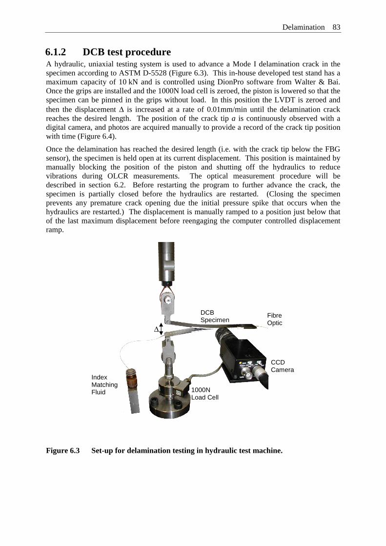
Delamination 83
6.1.2 DCB test procedure A hydraulic, uniaxial testing system is used to advance a Mode I delamination crack in the specimen according to ASTM D-5528 (Figure 6.3). This in-house developed test stand has a maximum capacity of 10 kN and is controlled using DionPro software from Walter & Bai. Once the grips are installed and the 1000N load cell is zeroed, the piston is lowered so that the specimen can be pinned in the grips without load. In this position the LVDT is zeroed and then the displacement Δ is increased at a rate of 0.01mm/min until the delamination crack reaches the desired length. The position of the crack tip a is continuously observed with a digital camera, and photos are acquired manually to provide a record of the crack tip position with time (Figure 6.4).
Once the delamination has reached the desired length (i.e. with the crack tip below the FBG sensor), the specimen is held open at its current displacement. This position is maintained by manually blocking the position of the piston and shutting off the hydraulics to reduce vibrations during OLCR measurements. The optical measurement procedure will be described in section 6.2. Before restarting the program to further advance the crack, the specimen is partially closed before the hydraulics are restarted. (Closing the specimen prevents any premature crack opening due the initial pressure spike that occurs when the hydraulics are restarted.) The displacement is manually ramped to a position just below that of the last maximum displacement before reengaging the computer controlled displacement ramp.
Figure 6.3 Set-up for delamination testing in hydraulic test machine.
CCD Camera
Fibre Optic
DCB Specimen
1000N Load Cell
Index Matching Fluid
Δ
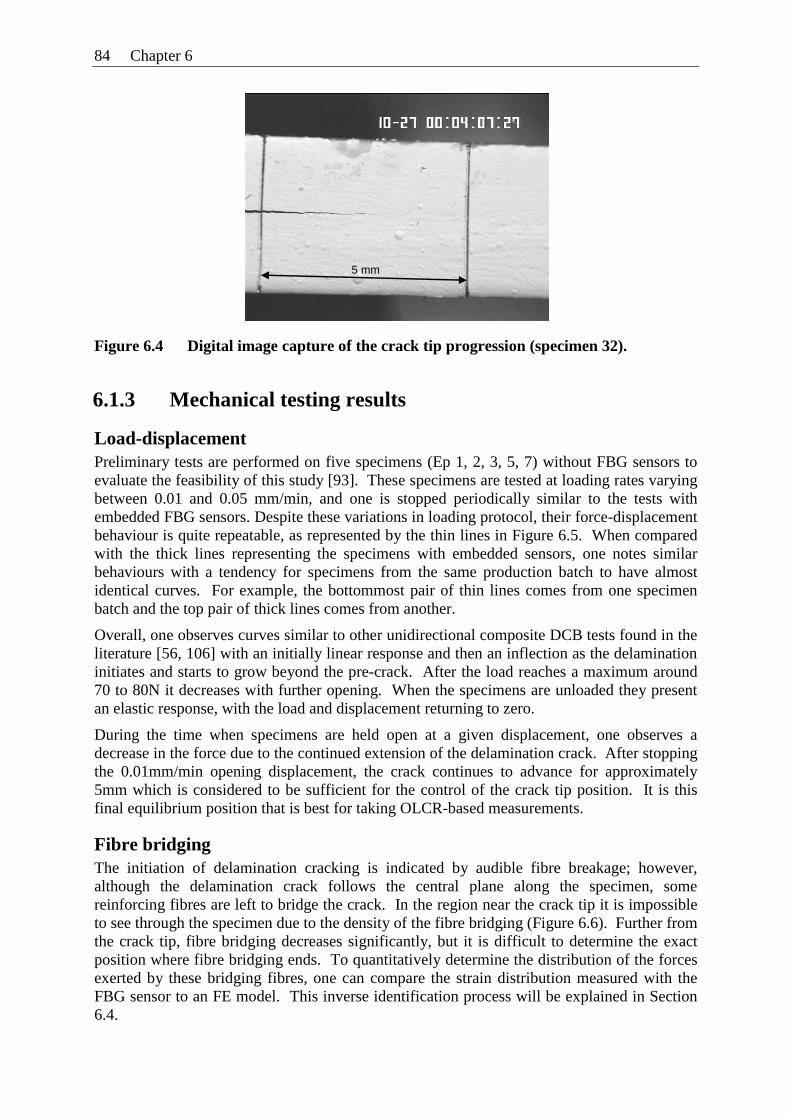
84 Chapter 6
Figure 6.4 Digital image capture of the crack tip progression (specimen 32).
6.1.3 Mechanical testing results
Load-displacement Preliminary tests are performed on five specimens (Ep 1, 2, 3, 5, 7) without FBG sensors to evaluate the feasibility of this study [93]. These specimens are tested at loading rates varying between 0.01 and 0.05 mm/min, and one is stopped periodically similar to the tests with embedded FBG sensors. Despite these variations in loading protocol, their force-displacement behaviour is quite repeatable, as represented by the thin lines in Figure 6.5. When compared with the thick lines representing the specimens with embedded sensors, one notes similar behaviours with a tendency for specimens from the same production batch to have almost identical curves. For example, the bottommost pair of thin lines comes from one specimen batch and the top pair of thick lines comes from another.
Overall, one observes curves similar to other unidirectional composite DCB tests found in the literature [56, 106] with an initially linear response and then an inflection as the delamination initiates and starts to grow beyond the pre-crack. After the load reaches a maximum around 70 to 80N it decreases with further opening. When the specimens are unloaded they present an elastic response, with the load and displacement returning to zero.
During the time when specimens are held open at a given displacement, one observes a decrease in the force due to the continued extension of the delamination crack. After stopping the 0.01mm/min opening displacement, the crack continues to advance for approximately 5mm which is considered to be sufficient for the control of the crack tip position. It is this final equilibrium position that is best for taking OLCR-based measurements.
Fibre bridging The initiation of delamination cracking is indicated by audible fibre breakage; however, although the delamination crack follows the central plane along the specimen, some reinforcing fibres are left to bridge the crack. In the region near the crack tip it is impossible to see through the specimen due to the density of the fibre bridging (Figure 6.6). Further from the crack tip, fibre bridging decreases significantly, but it is difficult to determine the exact position where fibre bridging ends. To quantitatively determine the distribution of the forces exerted by these bridging fibres, one can compare the strain distribution measured with the FBG sensor to an FE model. This inverse identification process will be explained in Section 6.4.
5 mm
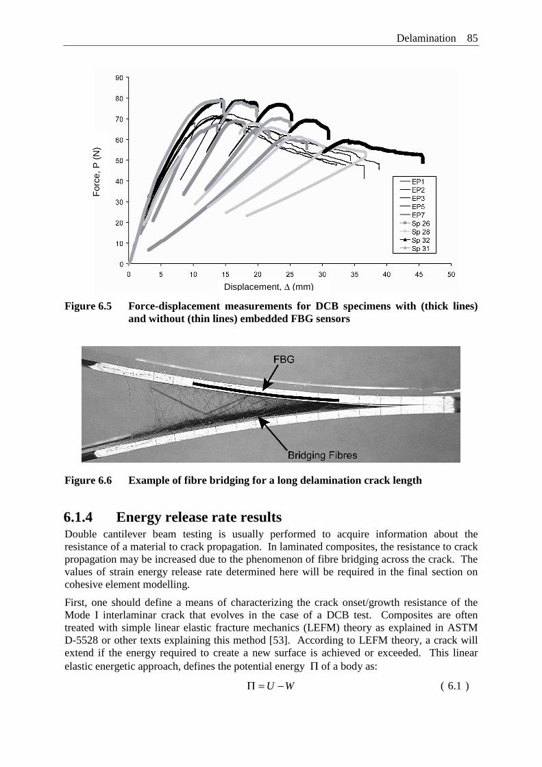
Delamination 85
Figure 6.5 Force-displacement measurements for DCB specimens with (thick lines) and without (thin lines) embedded FBG sensors
Figure 6.6 Example of fibre bridging for a long delamination crack length
6.1.4 Energy release rate results Double cantilever beam testing is usually performed to acquire information about the resistance of a material to crack propagation. In laminated composites, the resistance to crack propagation may be increased due to the phenomenon of fibre bridging across the crack. The values of strain energy release rate determined here will be required in the final section on cohesive element modelling.
First, one should define a means of characterizing the crack onset/growth resistance of the Mode I interlaminar crack that evolves in the case of a DCB test. Composites are often treated with simple linear elastic fracture mechanics (LEFM) theory as explained in ASTM D-5528 or other texts explaining this method [53]. According to LEFM theory, a crack will extend if the energy required to create a new surface is achieved or exceeded. This linear elastic energetic approach, defines the potential energy Π of a body as:
WU −=Π ( 6.1 )
For
ce, P
(N
)
Displacement, Δ (mm)
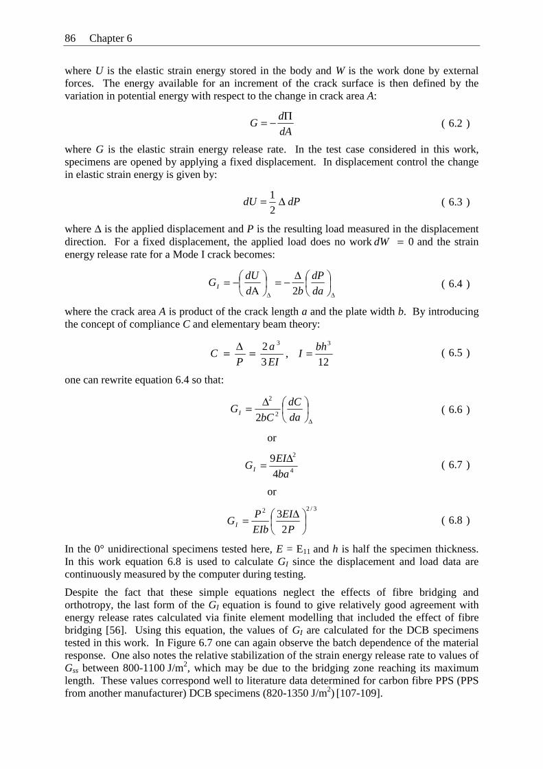
86 Chapter 6
where U is the elastic strain energy stored in the body and W is the work done by external forces. The energy available for an increment of the crack surface is then defined by the variation in potential energy with respect to the change in crack area A:
where G is the elastic strain energy release rate. In the test case considered in this work, specimens are opened by applying a fixed displacement. In displacement control the change in elastic strain energy is given by:
where Δ is the applied displacement and P is the resulting load measured in the displacement direction. For a fixed displacement, the applied load does no work 0=dW and the strain energy release rate for a Mode I crack becomes:
where the crack area A is product of the crack length a and the plate width b. By introducing the concept of compliance C and elementary beam theory:
one can rewrite equation 6.4 so that:
In the 0° unidirectional specimens tested here, E = E11 and h is half the specimen thickness. In this work equation 6.8 is used to calculate GI since the displacement and load data are continuously measured by the computer during testing.
Despite the fact that these simple equations neglect the effects of fibre bridging and orthotropy, the last form of the GI equation is found to give relatively good agreement with energy release rates calculated via finite element modelling that included the effect of fibre bridging [56]. Using this equation, the values of GI are calculated for the DCB specimens tested in this work. In Figure 6.7 one can again observe the batch dependence of the material response. One also notes the relative stabilization of the strain energy release rate to values of Gss between 800-1100 J/m2, which may be due to the bridging zone reaching its maximum length. These values correspond well to literature data determined for carbon fibre PPS (PPS from another manufacturer) DCB specimens (820-1350 J/m2) [107-109].
dA
dG
Π−= ( 6.2 )
dPdU Δ=2
1 ( 6.3 )
ΔΔ⎟⎠⎞
⎜⎝⎛Δ−=⎟
⎠⎞
⎜⎝⎛
Α−=
da
dP
bd
dUGI 2
( 6.4 )
EI
a
PC
32 3
=Δ= , 12
3bhI = ( 6.5 )
Δ⎟⎠⎞
⎜⎝⎛Δ=
da
dC
bCGI 2
2
2 ( 6.6 )
or
4
2
4
9
ba
EIGI
Δ= ( 6.7 )
or
3/22
2
3⎟⎠⎞
⎜⎝⎛ Δ=
P
EI
EIb
PGI ( 6.8 )
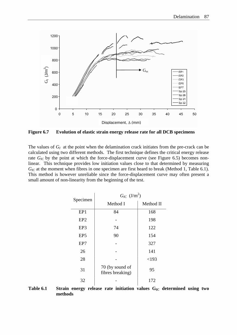
Delamination 87
Figure 6.7 Evolution of elastic strain energy release rate for all DCB specimens
The values of GI at the point when the delamination crack initiates from the pre-crack can be calculated using two different methods. The first technique defines the critical energy release rate GIC by the point at which the force-displacement curve (see Figure 6.5) becomes non-linear. This technique provides low initiation values close to that determined by measuring GIC at the moment when fibres in one specimen are first heard to break (Method 1, Table 6.1). This method is however unreliable since the force-displacement curve may often present a small amount of non-linearity from the beginning of the test.
GIC (J/m2) Specimen
Method I Method II
EP1 84 168
EP2 - 198
EP3 74 122
EP5 90 154
EP7 - 327
26 - 141
28 - <193
31 70 (by sound of fibres breaking)
95
32 - 172
Table 6.1 Strain energy release rate initiation values GIC determined using two methods
GI
(J/m
2 )
Displacement, Δ (mm)
Gss
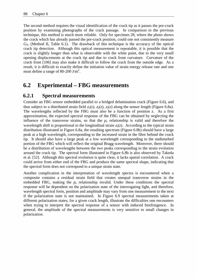
88 Chapter 6
The second method requires the visual identification of the crack tip as it passes the pre-crack position by examining photographs of the crack passage. In comparison to the previous technique, this method is much more reliable. Only for specimen 28, where the photo shows the crack which has already passed the pre-crack position, could one not consistently measure GIC (Method II, Table 6.1). The drawback of this technique is the accuracy of the optical crack tip detection. Although this optical measurement is repeatable, it is possible that the crack is slightly longer than what is observable with the white paint, due to the very small opening displacements at the crack tip and due to crack front curvature. Curvature of the crack front [106] may also make it difficult to follow the crack from the outside edge. As a result, it is difficult to exactly define the initiation value of strain energy release rate and one must define a range of 80-200 J/m2.
6.2 Experimental – FBG measurements
6.2.1 Spectral measurements Consider an FBG sensor embedded parallel to a bridged delamination crack (Figure 6.6), and thus subject to a distributed strain field εx(z), εy(z), εz(z) along the sensor length (Figure 6.8a). The wavelengths reflected by the FBG must also be a function of position z. As a first approximation, the expected spectral response of the FBG can be obtained by neglecting the influence of the transverse strains, so that the pe relationship is valid and therefore the wavelength shift is proportional to the longitudinal strain εz(z). According to the typical strain distribution illustrated in Figure 6.8a, the resulting spectrum (Figure 6.8b) should have a large peak at a high wavelength, corresponding to the increased strain in the fibre behind the crack tip. It should also have a large peak at a low wavelength corresponding to the undisturbed portion of the FBG which will reflect the original Bragg wavelength. Moreover, there should be a distribution of wavelengths between the two peaks corresponding to the strain evolution around the crack tip. The spectral form illustrated in Figure 6.8b is also observed by Takeda et al. [52]. Although this spectral evolution is quite clear, it lacks spatial correlation. A crack could arrive from either end of the FBG and produce the same spectral shape, indicating that the spectral form does not correspond to a unique strain state.
Another complication in the interpretation of wavelength spectra is encountered when a composite contains a residual strain field that creates unequal transverse strains in the embedded FBG, making the pe relationship invalid. Under these conditions the spectral response will be dependent on the polarization state of the interrogating light, and therefore, wavelength spectral form, position and amplitude may vary from one measurement to the next if the polarization state is not maintained. In Figure 6.9 spectral measurements taken at different polarization states, for a given crack length, illustrate the difficulties one encounters when trying to interpret the spectral response of a sensor with induced birefringence. In general, the amplitude of the spectral measurements is very sensitive to small changes in polarization.
Delamination 89
Figure 6.8 a) Schematic of a longitudinal strain (εz) distribution in an FBG embedded at a distance of 0.26 mm parallel to the delamination plane as shown in insert b) Actual spectral distribution measured for a given crack length in specimen 28.
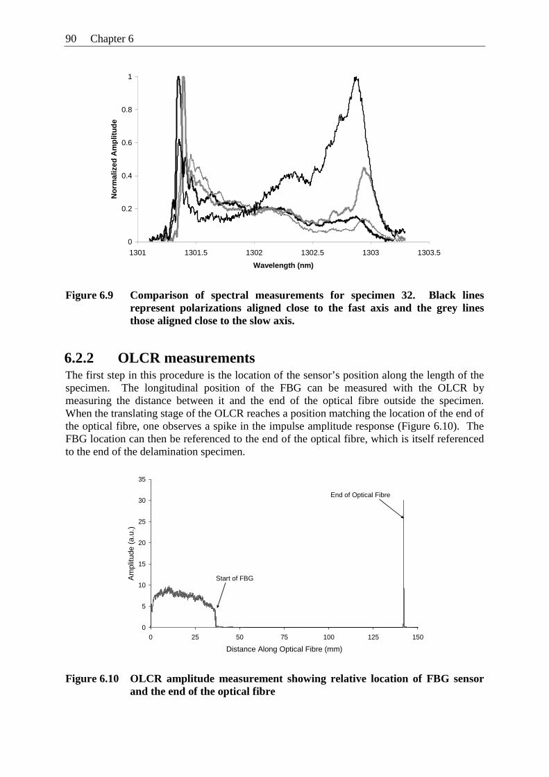
90 Chapter 6
0
0.2
0.4
0.6
0.8
1
1301 1301.5 1302 1302.5 1303 1303.5
Wavelength (nm)
No
rmal
ized
Am
plit
ud
e
Figure 6.9 Comparison of spectral measurements for specimen 32. Black lines represent polarizations aligned close to the fast axis and the grey lines those aligned close to the slow axis.
6.2.2 OLCR measurements The first step in this procedure is the location of the sensor’s position along the length of the specimen. The longitudinal position of the FBG can be measured with the OLCR by measuring the distance between it and the end of the optical fibre outside the specimen. When the translating stage of the OLCR reaches a position matching the location of the end of the optical fibre, one observes a spike in the impulse amplitude response (Figure 6.10). The FBG location can then be referenced to the end of the optical fibre, which is itself referenced to the end of the delamination specimen.
0
5
10
15
20
25
30
35
0 25 50 75 100 125 150
Distance Along Optical Fibre (mm)
Am
plitu
de (
a.u.
)
Start of FBG
End of Optical Fibre
Figure 6.10 OLCR amplitude measurement showing relative location of FBG sensor and the end of the optical fibre
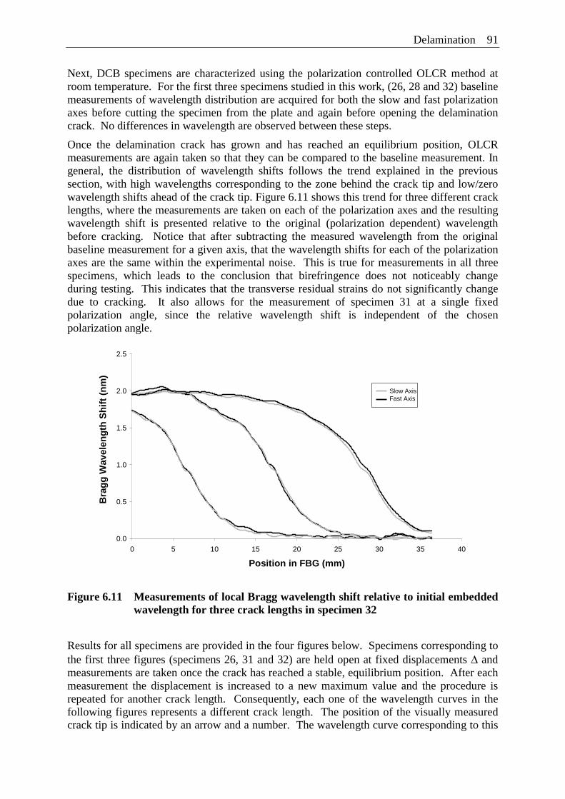
Delamination 91
Next, DCB specimens are characterized using the polarization controlled OLCR method at room temperature. For the first three specimens studied in this work, (26, 28 and 32) baseline measurements of wavelength distribution are acquired for both the slow and fast polarization axes before cutting the specimen from the plate and again before opening the delamination crack. No differences in wavelength are observed between these steps.
Once the delamination crack has grown and has reached an equilibrium position, OLCR measurements are again taken so that they can be compared to the baseline measurement. In general, the distribution of wavelength shifts follows the trend explained in the previous section, with high wavelengths corresponding to the zone behind the crack tip and low/zero wavelength shifts ahead of the crack tip. Figure 6.11 shows this trend for three different crack lengths, where the measurements are taken on each of the polarization axes and the resulting wavelength shift is presented relative to the original (polarization dependent) wavelength before cracking. Notice that after subtracting the measured wavelength from the original baseline measurement for a given axis, that the wavelength shifts for each of the polarization axes are the same within the experimental noise. This is true for measurements in all three specimens, which leads to the conclusion that birefringence does not noticeably change during testing. This indicates that the transverse residual strains do not significantly change due to cracking. It also allows for the measurement of specimen 31 at a single fixed polarization angle, since the relative wavelength shift is independent of the chosen polarization angle.
0.0
0.5
1.0
1.5
2.0
2.5
0 5 10 15 20 25 30 35 40
Position in FBG (mm)
Bra
gg
Wav
elen
gth
Sh
ift
(nm
)
Slow AxisFast Axis
Figure 6.11 Measurements of local Bragg wavelength shift relative to initial embedded wavelength for three crack lengths in specimen 32
Results for all specimens are provided in the four figures below. Specimens corresponding to the first three figures (specimens 26, 31 and 32) are held open at fixed displacements Δ and measurements are taken once the crack has reached a stable, equilibrium position. After each measurement the displacement is increased to a new maximum value and the procedure is repeated for another crack length. Consequently, each one of the wavelength curves in the following figures represents a different crack length. The position of the visually measured crack tip is indicated by an arrow and a number. The wavelength curve corresponding to this
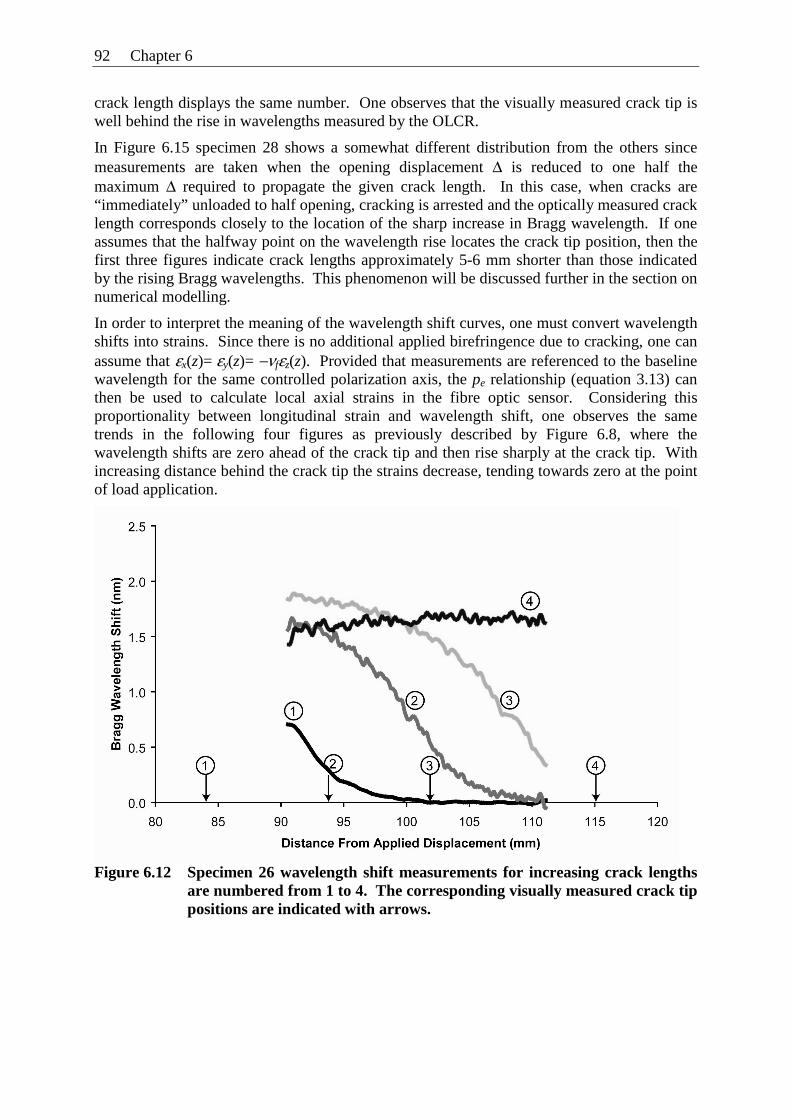
92 Chapter 6
crack length displays the same number. One observes that the visually measured crack tip is well behind the rise in wavelengths measured by the OLCR.
In Figure 6.15 specimen 28 shows a somewhat different distribution from the others since measurements are taken when the opening displacement Δ is reduced to one half the maximum Δ required to propagate the given crack length. In this case, when cracks are “immediately” unloaded to half opening, cracking is arrested and the optically measured crack length corresponds closely to the location of the sharp increase in Bragg wavelength. If one assumes that the halfway point on the wavelength rise locates the crack tip position, then the first three figures indicate crack lengths approximately 5-6 mm shorter than those indicated by the rising Bragg wavelengths. This phenomenon will be discussed further in the section on numerical modelling.
In order to interpret the meaning of the wavelength shift curves, one must convert wavelength shifts into strains. Since there is no additional applied birefringence due to cracking, one can assume that εx(z)= εy(z)= −νfεz(z). Provided that measurements are referenced to the baseline wavelength for the same controlled polarization axis, the pe relationship (equation 3.13) can then be used to calculate local axial strains in the fibre optic sensor. Considering this proportionality between longitudinal strain and wavelength shift, one observes the same trends in the following four figures as previously described by Figure 6.8, where the wavelength shifts are zero ahead of the crack tip and then rise sharply at the crack tip. With increasing distance behind the crack tip the strains decrease, tending towards zero at the point of load application.
Figure 6.12 Specimen 26 wavelength shift measurements for increasing crack lengths
are numbered from 1 to 4. The corresponding visually measured crack tip positions are indicated with arrows.
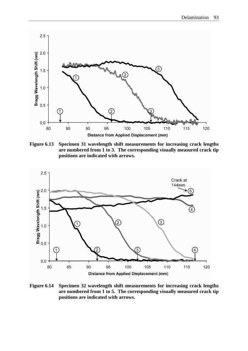
Delamination 93
Figure 6.13 Specimen 31 wavelength shift measurements for increasing crack lengths
are numbered from 1 to 3. The corresponding visually measured crack tip positions are indicated with arrows.
Figure 6.14 Specimen 32 wavelength shift measurements for increasing crack lengths are numbered from 1 to 5. The corresponding visually measured crack tip positions are indicated with arrows.
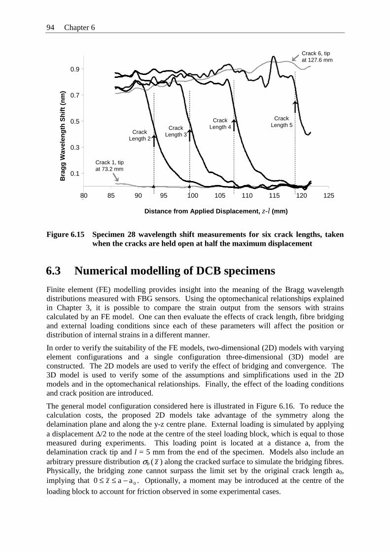
94 Chapter 6
Figure 6.15 Specimen 28 wavelength shift measurements for six crack lengths, taken when the cracks are held open at half the maximum displacement
6.3 Numerical modelling of DCB specimens
Finite element (FE) modelling provides insight into the meaning of the Bragg wavelength distributions measured with FBG sensors. Using the optomechanical relationships explained in Chapter 3, it is possible to compare the strain output from the sensors with strains calculated by an FE model. One can then evaluate the effects of crack length, fibre bridging and external loading conditions since each of these parameters will affect the position or distribution of internal strains in a different manner.
In order to verify the suitability of the FE models, two-dimensional (2D) models with varying element configurations and a single configuration three-dimensional (3D) model are constructed. The 2D models are used to verify the effect of bridging and convergence. The 3D model is used to verify some of the assumptions and simplifications used in the 2D models and in the optomechanical relationships. Finally, the effect of the loading conditions and crack position are introduced.
The general model configuration considered here is illustrated in Figure 6.16. To reduce the calculation costs, the proposed 2D models take advantage of the symmetry along the delamination plane and along the y-z centre plane. External loading is simulated by applying a displacement Δ/2 to the node at the centre of the steel loading block, which is equal to those measured during experiments. This loading point is located at a distance a, from the delamination crack tip and l = 5 mm from the end of the specimen. Models also include an arbitrary pressure distribution σb ( z ) along the cracked surface to simulate the bridging fibres. Physically, the bridging zone cannot surpass the limit set by the original crack length a0, implying that 0aa0 −≤≤ z . Optionally, a moment may be introduced at the centre of the
loading block to account for friction observed in some experimental cases.
0.1
0.3
0.5
0.7
0.9
80 85 90 95 100 105 110 115 120 125
Distance from Applied Displacement, z-l (mm)
Bra
gg
Wav
elen
gth
Sh
ift
(nm
)
Crack 1, tip at 73.2 mm
Crack Length 2
Crack Length 3
Crack Length 4
Crack 6, tip at 127.6 mm
Crack Length 5
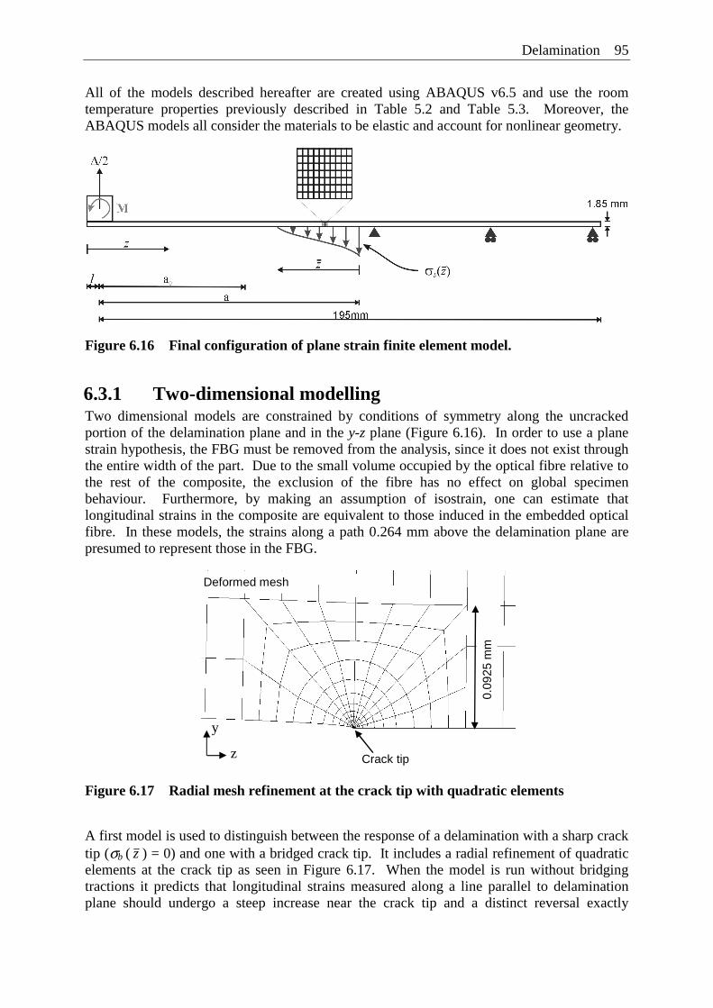
Delamination 95
All of the models described hereafter are created using ABAQUS v6.5 and use the room temperature properties previously described in Table 5.2 and Table 5.3. Moreover, the ABAQUS models all consider the materials to be elastic and account for nonlinear geometry.
Figure 6.16 Final configuration of plane strain finite element model.
6.3.1 Two-dimensional modelling Two dimensional models are constrained by conditions of symmetry along the uncracked portion of the delamination plane and in the y-z plane (Figure 6.16). In order to use a plane strain hypothesis, the FBG must be removed from the analysis, since it does not exist through the entire width of the part. Due to the small volume occupied by the optical fibre relative to the rest of the composite, the exclusion of the fibre has no effect on global specimen behaviour. Furthermore, by making an assumption of isostrain, one can estimate that longitudinal strains in the composite are equivalent to those induced in the embedded optical fibre. In these models, the strains along a path 0.264 mm above the delamination plane are presumed to represent those in the FBG.
Figure 6.17 Radial mesh refinement at the crack tip with quadratic elements
A first model is used to distinguish between the response of a delamination with a sharp crack tip (σb ( z ) = 0) and one with a bridged crack tip. It includes a radial refinement of quadratic elements at the crack tip as seen in Figure 6.17. When the model is run without bridging tractions it predicts that longitudinal strains measured along a line parallel to delamination plane should undergo a steep increase near the crack tip and a distinct reversal exactly
Deformed mesh
0.09
25 m
m
z
y
Crack tip
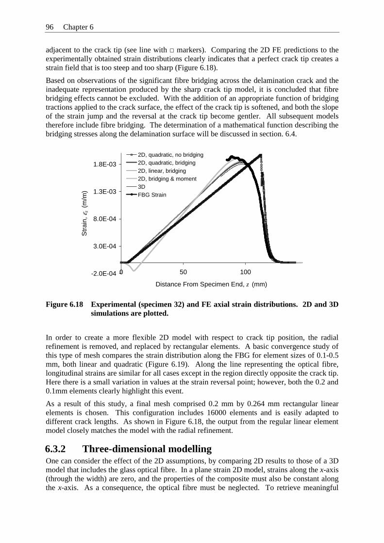
96 Chapter 6
adjacent to the crack tip (see line with □ markers). Comparing the 2D FE predictions to the experimentally obtained strain distributions clearly indicates that a perfect crack tip creates a strain field that is too steep and too sharp (Figure 6.18).
Based on observations of the significant fibre bridging across the delamination crack and the inadequate representation produced by the sharp crack tip model, it is concluded that fibre bridging effects cannot be excluded. With the addition of an appropriate function of bridging tractions applied to the crack surface, the effect of the crack tip is softened, and both the slope of the strain jump and the reversal at the crack tip become gentler. All subsequent models therefore include fibre bridging. The determination of a mathematical function describing the bridging stresses along the delamination surface will be discussed in section. 6.4.
-2.0E-04
3.0E-04
8.0E-04
1.3E-03
1.8E-03
0 50 100
Distance From Specimen End, z (mm)
Str
ain,
εz (
m/m
)
2D, quadratic, no bridging2D, quadratic, bridging2D, linear, bridging2D, bridging & moment3DFBG Strain
Figure 6.18 Experimental (specimen 32) and FE axial strain distributions. 2D and 3D simulations are plotted.
In order to create a more flexible 2D model with respect to crack tip position, the radial refinement is removed, and replaced by rectangular elements. A basic convergence study of this type of mesh compares the strain distribution along the FBG for element sizes of 0.1-0.5 mm, both linear and quadratic (Figure 6.19). Along the line representing the optical fibre, longitudinal strains are similar for all cases except in the region directly opposite the crack tip. Here there is a small variation in values at the strain reversal point; however, both the 0.2 and 0.1mm elements clearly highlight this event.
As a result of this study, a final mesh comprised 0.2 mm by 0.264 mm rectangular linear elements is chosen. This configuration includes 16000 elements and is easily adapted to different crack lengths. As shown in Figure 6.18, the output from the regular linear element model closely matches the model with the radial refinement.
6.3.2 Three-dimensional modelling One can consider the effect of the 2D assumptions, by comparing 2D results to those of a 3D model that includes the glass optical fibre. In a plane strain 2D model, strains along the x-axis (through the width) are zero, and the properties of the composite must also be constant along the x-axis. As a consequence, the optical fibre must be neglected. To retrieve meaningful
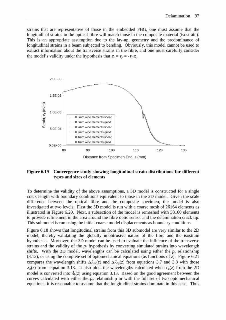
Delamination 97
strains that are representative of those in the embedded FBG, one must assume that the longitudinal strains in the optical fibre will match those in the composite material (isostrain). This is an appropriate assumption due to the lay-up, geometry and the predominance of longitudinal strains in a beam subjected to bending. Obviously, this model cannot be used to extract information about the transverse strains in the fibre, and one must carefully consider the model’s validity under the hypothesis that εx = εy ≈ -νf εz.
Figure 6.19 Convergence study showing longitudinal strain distributions for different types and sizes of elements
To determine the validity of the above assumptions, a 3D model is constructed for a single crack length with boundary conditions equivalent to those in the 2D model. Given the scale difference between the optical fibre and the composite specimen, the model is also investigated at two levels. First the 3D model is run with a coarse mesh of 26164 elements as illustrated in Figure 6.20. Next, a subsection of the model is remeshed with 38160 elements to provide refinement in the area around the fibre optic sensor and the delamination crack tip. This submodel is run using the initial coarse model displacements as boundary conditions.
Figure 6.18 shows that longitudinal strains from this 3D submodel are very similar to the 2D model, thereby validating the globally unobtrusive nature of the fibre and the isostrain hypothesis. Moreover, the 3D model can be used to evaluate the influence of the transverse strains and the validity of the pe hypothesis by converting simulated strains into wavelength shifts. With the 3D model, wavelengths can be calculated using either the pe relationship (3.13), or using the complete set of optomechanical equations (as functions of z). Figure 6.21 compares the wavelength shifts Δλbx(z) and Δλby(z) from equations 3.7 and 3.8 with those λb(z) from equation 3.13. It also plots the wavelengths calculated when εz(z) from the 2D model is converted into λb(z) using equation 3.13. Based on the good agreement between the curves calculated with either the pe relationship or with the full set of two optomechanical equations, it is reasonable to assume that the longitudinal strains dominate in this case. Thus
0.0E+00
5.0E-04
1.0E-03
1.5E-03
2.0E-03
80 90 100 110 120 130
Position From End of Specimen, a+l (mm)
Str
ain
ε z (
m/m
)
0.5mm wide elements linear
0.5mm wide elements quad
0.2mm wide elements linear
0.2mm wide elements quad
0.1mm wide elements linear
0.1mm wide elements quad
Distance from Specimen End, z (mm)
Str
ain,
εz
(m/m
)
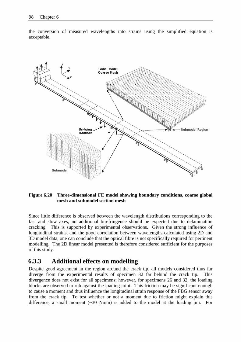
98 Chapter 6
the conversion of measured wavelengths into strains using the simplified equation is acceptable.
Figure 6.20 Three-dimensional FE model showing boundary conditions, coarse global mesh and submodel section mesh
Since little difference is observed between the wavelength distributions corresponding to the fast and slow axes, no additional birefringence should be expected due to delamination cracking. This is supported by experimental observations. Given the strong influence of longitudinal strains, and the good correlation between wavelengths calculated using 2D and 3D model data, one can conclude that the optical fibre is not specifically required for pertinent modelling. The 2D linear model presented is therefore considered sufficient for the purposes of this study.
6.3.3 Additional effects on modelling Despite good agreement in the region around the crack tip, all models considered thus far diverge from the experimental results of specimen 32 far behind the crack tip. This divergence does not exist for all specimens; however, for specimens 26 and 32, the loading blocks are observed to rub against the loading joint. This friction may be significant enough to cause a moment and thus influence the longitudinal strain response of the FBG sensor away from the crack tip. To test whether or not a moment due to friction might explain this difference, a small moment (~30 Nmm) is added to the model at the loading pin. For
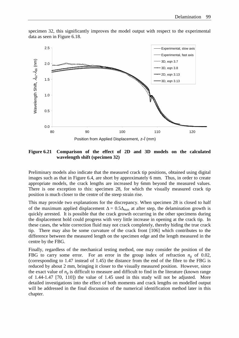
Delamination 99
specimen 32, this significantly improves the model output with respect to the experimental data as seen in Figure 6.18.
Figure 6.21 Comparison of the effect of 2D and 3D models on the calculated wavelength shift (specimen 32)
Preliminary models also indicate that the measured crack tip positions, obtained using digital images such as that in Figure 6.4, are short by approximately 6 mm. Thus, in order to create appropriate models, the crack lengths are increased by 6mm beyond the measured values. There is one exception to this: specimen 28, for which the visually measured crack tip position is much closer to the centre of the steep strain rise.
This may provide two explanations for the discrepancy. When specimen 28 is closed to half of the maximum applied displacement Δ = 0.5Δmax at after step, the delamination growth is quickly arrested. It is possible that the crack growth occurring in the other specimens during the displacement hold could progress with very little increase in opening at the crack tip. In these cases, the white correction fluid may not crack completely, thereby hiding the true crack tip. There may also be some curvature of the crack front [106] which contributes to the difference between the measured length on the specimen edge and the length measured in the centre by the FBG.
Finally, regardless of the mechanical testing method, one may consider the position of the FBG to carry some error. For an error in the group index of refraction ng of 0.02, (corresponding to 1.47 instead of 1.45) the distance from the end of the fibre to the FBG is reduced by about 2 mm, bringing it closer to the visually measured position. However, since the exact value of ng is difficult to measure and difficult to find in the literature (known range of 1.44-1.47 [70, 110]) the value of 1.45 used in this study will not be adjusted. More detailed investigations into the effect of both moments and crack lengths on modelled output will be addressed in the final discussion of the numerical identification method later in this chapter.
0.0
0.5
1.0
1.5
2.0
2.5
80 90 100 110 120
Position from Applied Displacement, z-l (mm)
Wav
elen
gth
Shi
ft, λ
bi-λ
Bi (
nm)
Experimental, slow axis Experimental, fast axis
3D, eqn 3.7
3D, eqn 3.8
2D, eqn 3.13
3D, eqn 3.13
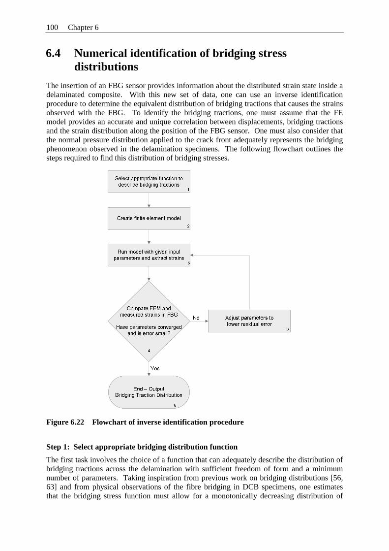
100 Chapter 6
6.4 Numerical identification of bridging stress distributions
The insertion of an FBG sensor provides information about the distributed strain state inside a delaminated composite. With this new set of data, one can use an inverse identification procedure to determine the equivalent distribution of bridging tractions that causes the strains observed with the FBG. To identify the bridging tractions, one must assume that the FE model provides an accurate and unique correlation between displacements, bridging tractions and the strain distribution along the position of the FBG sensor. One must also consider that the normal pressure distribution applied to the crack front adequately represents the bridging phenomenon observed in the delamination specimens. The following flowchart outlines the steps required to find this distribution of bridging stresses.
Figure 6.22 Flowchart of inverse identification procedure
Step 1: Select appropriate bridging distribution function
The first task involves the choice of a function that can adequately describe the distribution of bridging tractions across the delamination with sufficient freedom of form and a minimum number of parameters. Taking inspiration from previous work on bridging distributions [56, 63] and from physical observations of the fibre bridging in DCB specimens, one estimates that the bridging stress function must allow for a monotonically decreasing distribution of
Delamination 101
stresses as the distance from the crack tip increases. To provide the function with significant flexibility, it is initially represented by a 4th order polynomial multiplied by an exponential; however, after various trials, it is observed that the output can be equally-well described with a first order polynomial multiplied by an exponential term:
where σb is the bridging stress normal to the delamination plane, z is the position from the crack tip and γ is the exponential parameter defining the degree of non-linearity of the bridging curve. The A1 constant defines the maximum stress at the crack tip σbmax and the ratio of A1 to A2 defines the maximum length maxz of the bridging zone such that:
Since these parameters have some physical meaning, one can also impose limits on their values. For example, the bridging length can not extend beyond the pre-crack tip position and can not be negative. Nor can the maximum stress be negative. In addition, the maximum stress cannot exceed the failure stress of the material. Finally, the bridging stresses should not exceed the maximum stress at 0=z thus implying a positive value of γ. A summary of these conditions is listed in Table 6.2
Parameter Condition
γ γ ≥ 0
A1 = σbmax 0 ≤ A1 ≤ Maximum Failure Stress
-A1/A2 = maxz 0 ≤ -A1/A2 ≤ a-a0
Table 6.2 Limits on parameters used in Equation 6.9.
Step 2: Creation of finite element model
In ABAQUS 6.5, the normal bridging tractions are modelled as a user-defined pressure distribution applied to the portion of the delamination surface between the crack tip and the pre-crack tip as illustrated in Figure 6.16. A Fortran subroutine linked to the model calculates the appropriate applied pressure based on the position z from the crack tip, Equation 6.9 and the choice of corresponding parameters γ, A1 and A2. The displacement of the loading blocks is given from the experimental tests, and corresponds to the particular crack length and specimen under consideration. Crack lengths are set at the visually inspected length +6mm as discussed in section 6.2.2. Without this increase in crack length, the measured strain distributions will be offset from those calculated by the model.
Step 3: Run model with chosen input parameters and extract FBG strains
A Matlab routine controls the execution of the FE model and subsequent optimization steps [95]. Initially, one inputs arbitrary values of the three parameters that fall within the previously discussed limits. Given the particular set of input parameters, Matlab calls the FE model and extracts the longitudinal strains along a node-path representing the core of the optical fibre sensor.
Trials for different crack lengths and different specimens have been run with values chosen to represent the distribution as a shallow curve with a low stress and long bridging length and as
( )zAAez zb 21)( += − γσ ( 6.9 )
2
1max
2
1 ,0A
Az
A
Ab −==
−σ ( 6.10 )
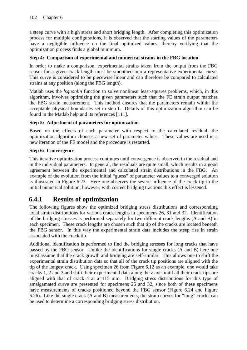
102 Chapter 6
a steep curve with a high stress and short bridging length. After completing this optimization process for multiple configurations, it is observed that the starting values of the parameters have a negligible influence on the final optimized values, thereby verifying that the optimization process finds a global minimum.
Step 4: Comparison of experimental and numerical strains in the FBG location
In order to make a comparison, experimental strains taken from the output from the FBG sensor for a given crack length must be smoothed into a representative experimental curve. This curve is considered to be piecewise linear and can therefore be compared to calculated strains at any position (along the FBG length).
Matlab uses the lsqnonlin function to solve nonlinear least-squares problems, which, in this algorithm, involves optimizing the given parameters such that the FE strain output matches the FBG strain measurement. This method ensures that the parameters remain within the acceptable physical boundaries set in step 1. Details of this optimization algorithm can be found in the Matlab help and its references [111].
Step 5: Adjustment of parameters for optimization
Based on the effects of each parameter with respect to the calculated residual, the optimization algorithm chooses a new set of parameter values. These values are used in a new iteration of the FE model and the procedure is restarted.
Step 6: Convergence
This iterative optimization process continues until convergence is observed in the residual and in the individual parameters. In general, the residuals are quite small, which results in a good agreement between the experimental and calculated strain distributions in the FBG. An example of the evolution from the initial “guess” of parameter values to a converged solution is illustrated in Figure 6.23. Here one observes the severe influence of the crack tip in the initial numerical solution; however, with correct bridging tractions this effect is lessened.
6.4.1 Results of optimization The following figures show the optimized bridging stress distributions and corresponding axial strain distributions for various crack lengths in specimens 26, 31 and 32. Identification of the bridging stresses is performed separately for two different crack lengths (A and B) in each specimen. These crack lengths are chosen such that tip of the cracks are located beneath the FBG sensor. In this way the experimental strain data includes the steep rise in strain associated with the crack tip.
Additional identification is performed to find the bridging stresses for long cracks that have passed by the FBG sensor. Unlike the identifications for single cracks (A and B) here one must assume that the crack growth and bridging are self-similar. This allows one to shift the experimental strain distribution data so that all of the crack tip positions are aligned with the tip of the longest crack. Using specimen 26 from Figure 6.12 as an example, one would take cracks 1, 2 and 3 and shift their experimental data along the z axis until all their crack tips are aligned with that of crack 4 at a=115 mm. Bridging stress distributions for this type of amalgamated curve are presented for specimens 26 and 32, since both of these specimens have measurements of cracks positioned beyond the FBG sensor (Figure 6.24 and Figure 6.26). Like the single crack (A and B) measurements, the strain curves for “long” cracks can be used to determine a corresponding bridging stress distribution.
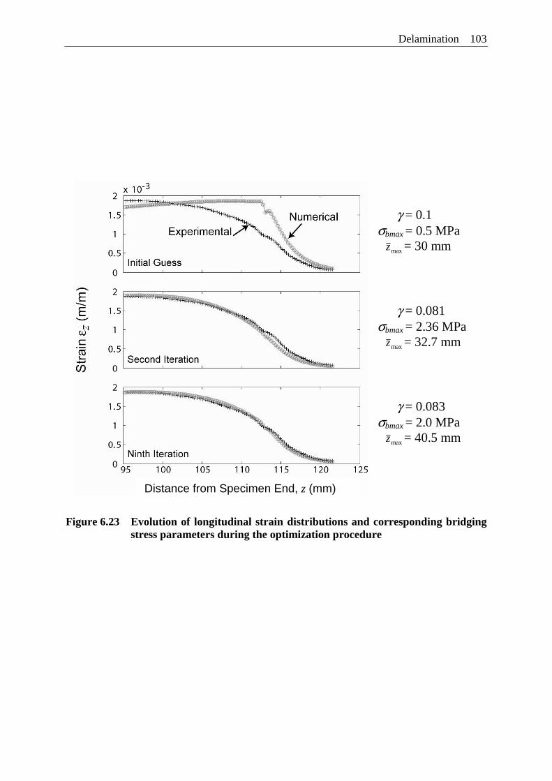
Delamination 103
Figure 6.23 Evolution of longitudinal strain distributions and corresponding bridging stress parameters during the optimization procedure
γ = 0.1 σbmax = 0.5 MPa maxz = 30 mm
γ = 0.081 σbmax = 2.36 MPa maxz = 32.7 mm
γ = 0.083 σbmax = 2.0 MPa maxz = 40.5 mm
Distance from Specimen End, z (mm)
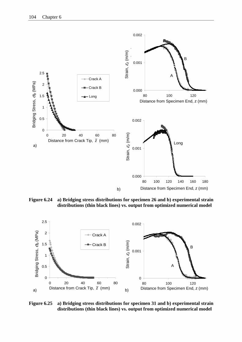
104 Chapter 6
Figure 6.24 a) Bridging stress distributions for specimen 26 and b) experimental strain distributions (thin black lines) vs. output from optimized numerical model
Figure 6.25 a) Bridging stress distributions for specimen 31 and b) experimental strain distributions (thin black lines) vs. output from optimized numerical model
0
0.001
0.002
80 100 120
Distance from Specimen End (mm)
Axi
al S
trai
n (m
/m)
0
0.5
1
1.5
2
2.5
0 20 40 60 80
Distance from Crack Tip (mm)
Bri
dg
ing
Str
ess
(MP
a)
Crack A
Crack BB
Distance from Specimen End, z (mm)
Str
ain,
ε z (
m/m
)
Distance from Crack Tip, z (mm)
Brid
ging
Str
ess,
σb
(MP
a)
A
a) b)
0.000
0.001
0.002
80 100 120 140 160 180
Distance from Specimen End (mm)
Axi
al S
trai
n (m
/m)
0.000
0.001
0.002
80 100 120
Distance from Specimen End (mm)
Axi
al S
trai
n (m
/m)
B
Long
Distance from Specimen End, z (mm)
Distance from Specimen End, z (mm)
Str
ain,
ε z (
m/m
) S
trai
n, ε z
(m
/m)
0
0.5
1
1.5
2
2.5
0 20 40 60 80
Distance from Crack Tip (mm)
Bri
dg
ing
Str
ess
(MP
a)
Crack A
Crack B
Composite
Distance from Crack Tip, z (mm)
Long
Brid
ging
Str
ess,
σb
(MP
a)
A
a)
b)
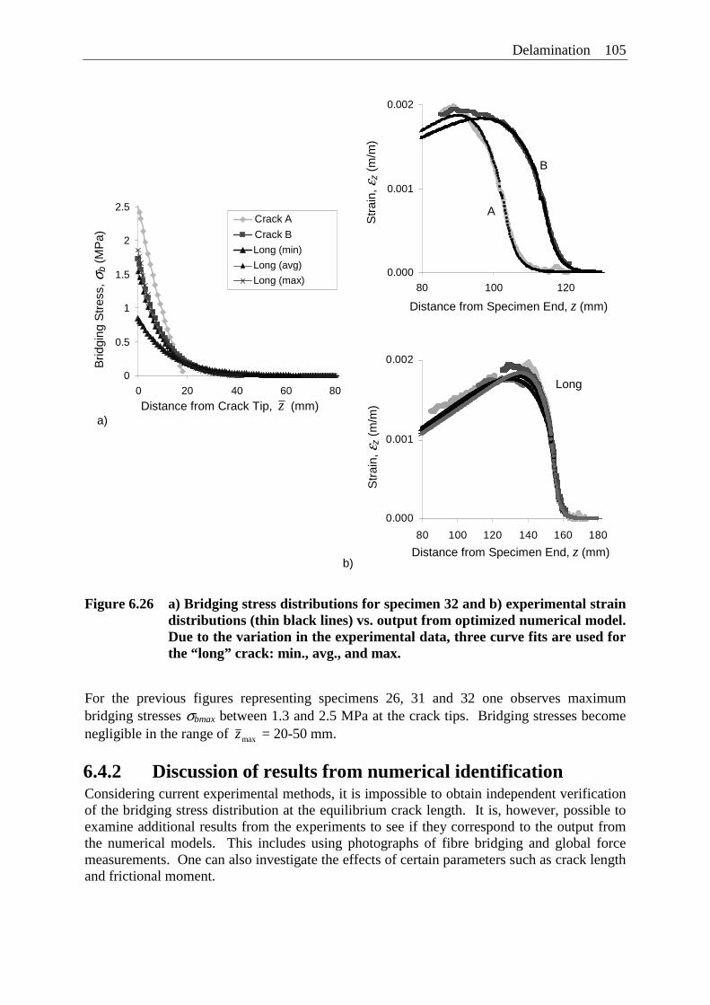
Delamination 105
Figure 6.26 a) Bridging stress distributions for specimen 32 and b) experimental strain distributions (thin black lines) vs. output from optimized numerical model. Due to the variation in the experimental data, three curve fits are used for the “long” crack: min., avg., and max.
For the previous figures representing specimens 26, 31 and 32 one observes maximum bridging stresses σbmax between 1.3 and 2.5 MPa at the crack tips. Bridging stresses become negligible in the range of maxz = 20-50 mm.
6.4.2 Discussion of results from numerical identification Considering current experimental methods, it is impossible to obtain independent verification of the bridging stress distribution at the equilibrium crack length. It is, however, possible to examine additional results from the experiments to see if they correspond to the output from the numerical models. This includes using photographs of fibre bridging and global force measurements. One can also investigate the effects of certain parameters such as crack length and frictional moment.
0
0.5
1
1.5
2
2.5
0 20 40 60 80
Distance from Crack Tip (mm)
Bri
dg
ing
Str
ess
(MP
a)
Crack A
Crack B
Composite (min)
Composite (avg)
Composite (max)0.000
0.001
0.002
80 100 120Distance from Specimen End (mm)
Axi
al s
trai
n (m
/m)
0.000
0.001
0.002
80 100 120 140 160 180
Distance from Specimen End (mm)
Axi
al S
trai
n (m
/m)
B
Long
Distance from Specimen End, z (mm)
Distance from Specimen End, z (mm)
Str
ain,
ε z (
m/m
) S
trai
n, ε z
(m
/m) Distance from Crack Tip, z (mm)
Long (min)
Long (avg)
Long (max)
Brid
ging
Str
ess,
σb
(MP
a)
A
a)
b)
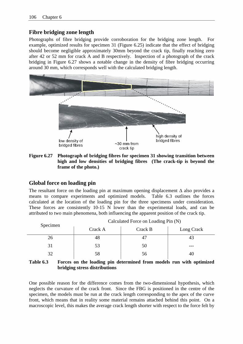
106 Chapter 6
Fibre bridging zone length Photographs of fibre bridging provide corroboration for the bridging zone length. For example, optimized results for specimen 31 (Figure 6.25) indicate that the effect of bridging should become negligible approximately 30mm beyond the crack tip, finally reaching zero after 42 or 52 mm for crack A and B respectively. Inspection of a photograph of the crack bridging in Figure 6.27 shows a notable change in the density of fibre bridging occurring around 30 mm, which corresponds well with the calculated bridging length.
Figure 6.27 Photograph of bridging fibres for specimen 31 showing transition between high and low densities of bridging fibres (The crack-tip is beyond the frame of the photo.)
Global force on loading pin The resultant force on the loading pin at maximum opening displacement Δ also provides a means to compare experiments and optimized models. Table 6.3 outlines the forces calculated at the location of the loading pin for the three specimens under consideration. These forces are consistently 10-15 N lower than the experimental loads, and can be attributed to two main phenomena, both influencing the apparent position of the crack tip.
Calculated Force on Loading Pin (N) Specimen
Crack A Crack B Long Crack
26 48 47 43
31 53 50 ---
32 58 56 40
Table 6.3 Forces on the loading pin determined from models run with optimized bridging stress distributions
One possible reason for the difference comes from the two-dimensional hypothesis, which neglects the curvature of the crack front. Since the FBG is positioned in the centre of the specimen, the models must be run at the crack length corresponding to the apex of the curve front, which means that in reality some material remains attached behind this point. On a macroscopic level, this makes the average crack length shorter with respect to the force felt by
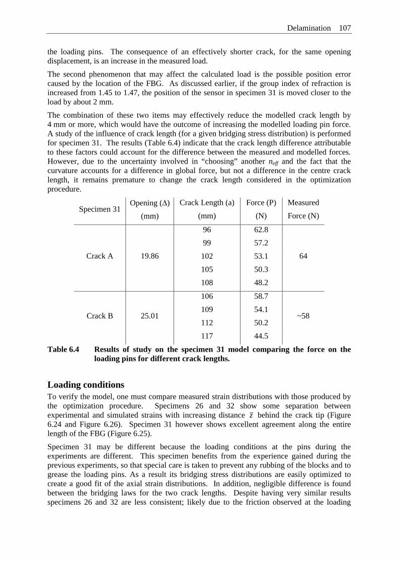
Delamination 107
the loading pins. The consequence of an effectively shorter crack, for the same opening displacement, is an increase in the measured load.
The second phenomenon that may affect the calculated load is the possible position error caused by the location of the FBG. As discussed earlier, if the group index of refraction is increased from 1.45 to 1.47, the position of the sensor in specimen 31 is moved closer to the load by about 2 mm.
The combination of these two items may effectively reduce the modelled crack length by 4 mm or more, which would have the outcome of increasing the modelled loading pin force. A study of the influence of crack length (for a given bridging stress distribution) is performed for specimen 31. The results (Table 6.4) indicate that the crack length difference attributable to these factors could account for the difference between the measured and modelled forces. However, due to the uncertainty involved in “choosing” another neff and the fact that the curvature accounts for a difference in global force, but not a difference in the centre crack length, it remains premature to change the crack length considered in the optimization procedure.
Specimen 31 Opening (Δ)
(mm)
Crack Length (a)
(mm)
Force (P)
(N)
Measured
Force (N)
96 62.8
99 57.2
102 53.1
105 50.3
Crack A 19.86
108 48.2
64
106 58.7
109 54.1
112 50.2 Crack B 25.01
117 44.5
~58
Table 6.4 Results of study on the specimen 31 model comparing the force on the loading pins for different crack lengths.
Loading conditions To verify the model, one must compare measured strain distributions with those produced by the optimization procedure. Specimens 26 and 32 show some separation between experimental and simulated strains with increasing distance z behind the crack tip (Figure 6.24 and Figure 6.26). Specimen 31 however shows excellent agreement along the entire length of the FBG (Figure 6.25).
Specimen 31 may be different because the loading conditions at the pins during the experiments are different. This specimen benefits from the experience gained during the previous experiments, so that special care is taken to prevent any rubbing of the blocks and to grease the loading pins. As a result its bridging stress distributions are easily optimized to create a good fit of the axial strain distributions. In addition, negligible difference is found between the bridging laws for the two crack lengths. Despite having very similar results specimens 26 and 32 are less consistent; likely due to the friction observed at the loading
108 Chapter 6
blocks which sometimes necessitates an adjustment of their position to keep them properly aligned.
To elucidate the potential effect of this friction, one may apply a moment around the loading pin as indicated in grey in Figure 6.16. An example of the results of this effort is provided for specimen 32 in Figure 6.28, where the moment has been defined as an optimizable parameter in the numerical identification process. The optimized moment for the three crack lengths ranges between 26-41 Nmm. With these results (Figure 6.28b) one observes considerable improvement in the axial strains away from the crack tip, where the maximum and slope of the distribution is most affected by the moment. In the region near the crack tip, clearly the geometry and the bridging have the greatest influence. A second improvement is achieved with the addition of the bridging moment: an increase in the calculated reaction force at the loading blocks. (Note that this would not improve the force for specimen 31 where no moment is necessary.) Both of these results are accomplished without a significant change in the bridging stress distributions.
6.5 Alternate method for describing bridging
A second method using cohesive elements in a new FE model is considered to simulate the effect of fibre bridging in the delamination specimen. This approach combines the domains of damage and fracture mechanics and has the advantage of modelling crack growth, by using elements that degrade and finally rupture as they are opened. This allows the delamination growth to be followed progressively, with the model determining its own final crack length.
In this section a second independent measurement of the bridging law is determined via the “J-integral approach”. It provides an alternative interpretation of the fibre bridging behaviour that can be compared with the results from section 6.4. To make this comparison, bridging laws (from both methods) are used to define the behaviour of cohesive elements in the new FE model. The cohesive element model then simulates crack growth progression and global force-displacement behaviour can be extracted.
6.5.1 Determination of bridging law using J-integral approach To define a bridging law, consider the schematic in Figure 6.29 below. In this figure the bridging fibres are represented by lines crossing the crack plane. Section 6.4 explained that these fibres could be represented by equivalent bridging stresses that were functions of their position z . In this section, the bridging stresses are defined with respect to the separation of the crack surfaces:
This function is assumed to be identical for every location along the bridging zone [112]. One may also assume that the bridging stresses will vanish when δ reaches the maximum separation limit δf, so that 0)( =fb δσ .
)(δσσ bb = ( 6.11 )
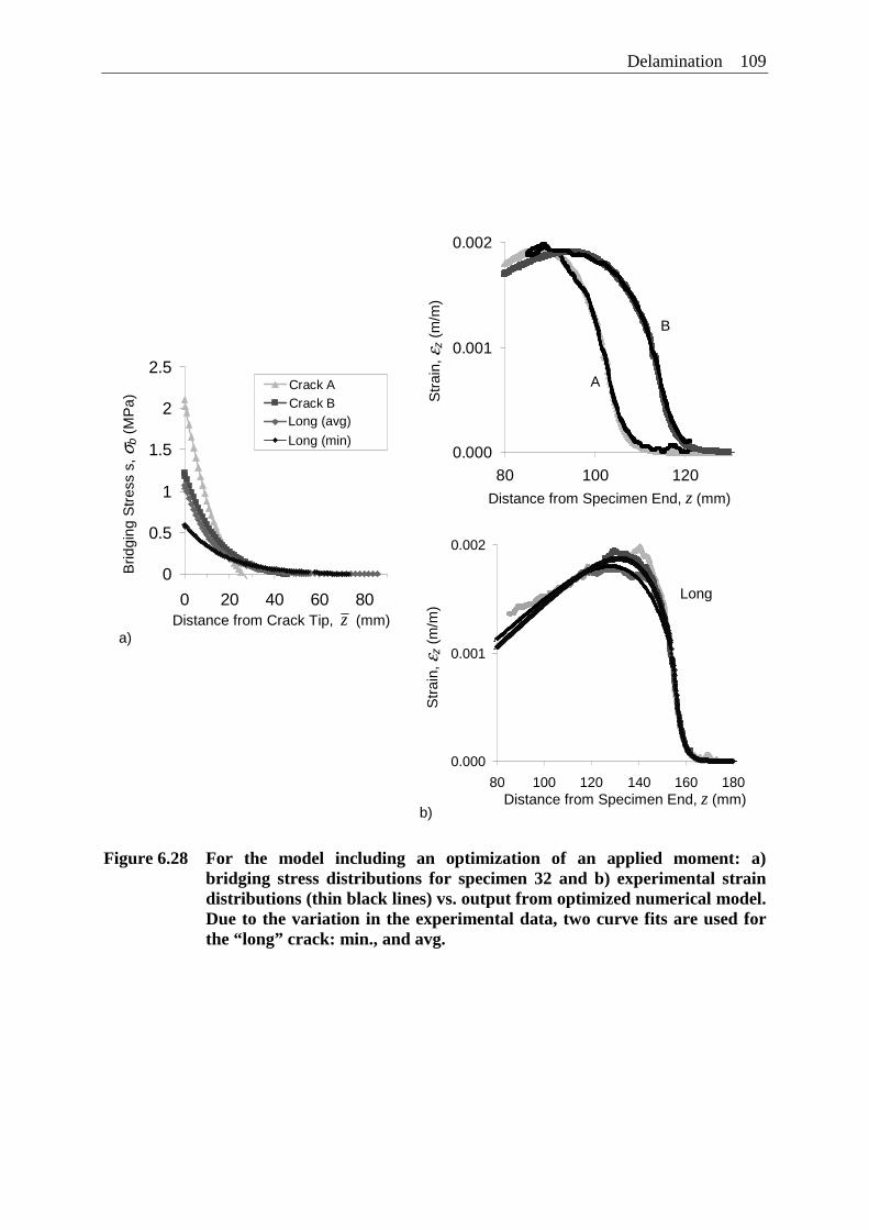
Delamination 109
Figure 6.28 For the model including an optimization of an applied moment: a) bridging stress distributions for specimen 32 and b) experimental strain distributions (thin black lines) vs. output from optimized numerical model. Due to the variation in the experimental data, two curve fits are used for the “long” crack: min., and avg.
0
0.5
1
1.5
2
2.5
0 20 40 60 80
Distance from crack-tip (mm)
Bri
dg
ing
Str
ess
(MP
a)
Crack ACrack B
Composite (avg)Composite (min)
0.000
0.001
0.002
80 100 120
Distance From Specimen End (mm)
Axi
al s
trai
n (m
/m)
0.000
0.001
0.002
80 100 120 140 160 180
Distance from Specimen End (mm)
Axi
al S
trai
n (
m/m
)
B
Long
Distance from Specimen End, z (mm)
Distance from Specimen End, z (mm)
Str
ain,
ε z (
m/m
) S
trai
n, ε z
(m
/m)
Distance from Crack Tip, z (mm)
Long (avg)
Long (min)
Brid
ging
Str
ess
s, σ
b (M
Pa)
A
a)
b)
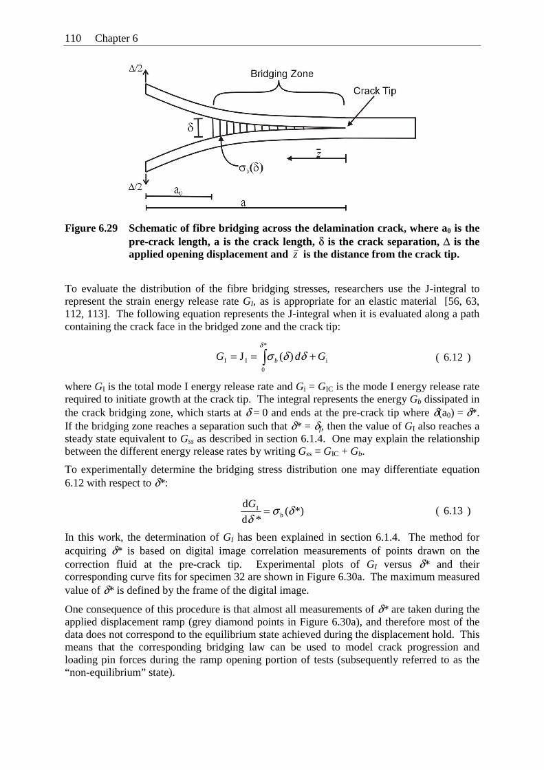
110 Chapter 6
Figure 6.29 Schematic of fibre bridging across the delamination crack, where a0 is the pre-crack length, a is the crack length, δ is the crack separation, Δ is the applied opening displacement and z is the distance from the crack tip.
To evaluate the distribution of the fibre bridging stresses, researchers use the J-integral to represent the strain energy release rate GI, as is appropriate for an elastic material [56, 63, 112, 113]. The following equation represents the J-integral when it is evaluated along a path containing the crack face in the bridged zone and the crack tip:
where GI is the total mode I energy release rate and Gi = GIC is the mode I energy release rate required to initiate growth at the crack tip. The integral represents the energy Gb dissipated in the crack bridging zone, which starts at δ = 0 and ends at the pre-crack tip where δ(a0) = δ*. If the bridging zone reaches a separation such that δ* = δf, then the value of GI also reaches a steady state equivalent to Gss as described in section 6.1.4. One may explain the relationship between the different energy release rates by writing Gss = GIC + Gb.
To experimentally determine the bridging stress distribution one may differentiate equation 6.12 with respect to δ*:
In this work, the determination of GI has been explained in section 6.1.4. The method for acquiring δ* is based on digital image correlation measurements of points drawn on the correction fluid at the pre-crack tip. Experimental plots of GI versus δ* and their corresponding curve fits for specimen 32 are shown in Figure 6.30a. The maximum measured value of δ* is defined by the frame of the digital image.
One consequence of this procedure is that almost all measurements of δ* are taken during the applied displacement ramp (grey diamond points in Figure 6.30a), and therefore most of the data does not correspond to the equilibrium state achieved during the displacement hold. This means that the corresponding bridging law can be used to model crack progression and loading pin forces during the ramp opening portion of tests (subsequently referred to as the “non-equilibrium” state).
i
*
0
II )( J GdG b +== ∫ δδσδ
( 6.12 )
*)( *d
d I δσδ b
G = ( 6.13 )
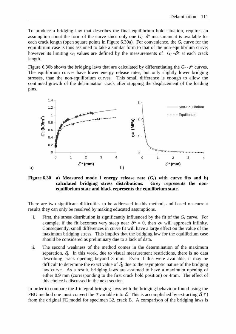
Delamination 111
To produce a bridging law that describes the final equilibrium hold situation, requires an assumption about the form of the curve since only one GI -δ* measurement is available for each crack length (open square points in Figure 6.30a). For convenience, the GI curve for the equilibrium case is thus assumed to take a similar form to that of the non-equilibrium curve; however its limiting GI values are defined by the measurements of GI -δ* at each crack length.
Figure 6.30b shows the bridging laws that are calculated by differentiating the GI -δ* curves. The equilibrium curves have lower energy release rates, but only slightly lower bridging stresses, than the non-equilibrium curves. This small difference is enough to allow the continued growth of the delamination crack after stopping the displacement of the loading pins.
a)
0
0.2
0.4
0.6
0.8
1
1.2
1.4
0 1 2 3 4
δ * (mm)
GI (
kJ/m
2 )
b)
0
1
2
3
0 1 2 3 4
δ * (mm)
σb (M
Pa)
Non-Equilibrium
Equilibrium
Figure 6.30 a) Measured mode I energy release rate (GI) with curve fits and b) calculated bridging stress distributions. Grey represents the non-equilibrium state and black represents the equilibrium state.
There are two significant difficulties to be addressed in this method, and based on current results they can only be resolved by making educated assumptions.
i. First, the stress distribution is significantly influenced by the fit of the GI curve. For example, if the fit becomes very steep near δ* = 0, then σb will approach infinity. Consequently, small differences in curve fit will have a large effect on the value of the maximum bridging stress. This implies that the bridging law for the equilibrium case should be considered as preliminary due to a lack of data.
ii. The second weakness of the method comes in the determination of the maximum separation, δf. In this work, due to visual measurement restrictions, there is no data describing crack opening beyond 3 mm. Even if this were available, it may be difficult to determine the exact value of δf, due to the asymptotic nature of the bridging law curve. As a result, bridging laws are assumed to have a maximum opening of either 0.9 mm (corresponding to the first crack hold position) or 4mm. The effect of this choice is discussed in the next section.
In order to compare the J-integral bridging laws with the bridging behaviour found using the FBG method one must convert the z variable into δ. This is accomplished by extracting δ( z ) from the original FE model for specimen 32, crack B. A comparison of the bridging laws is
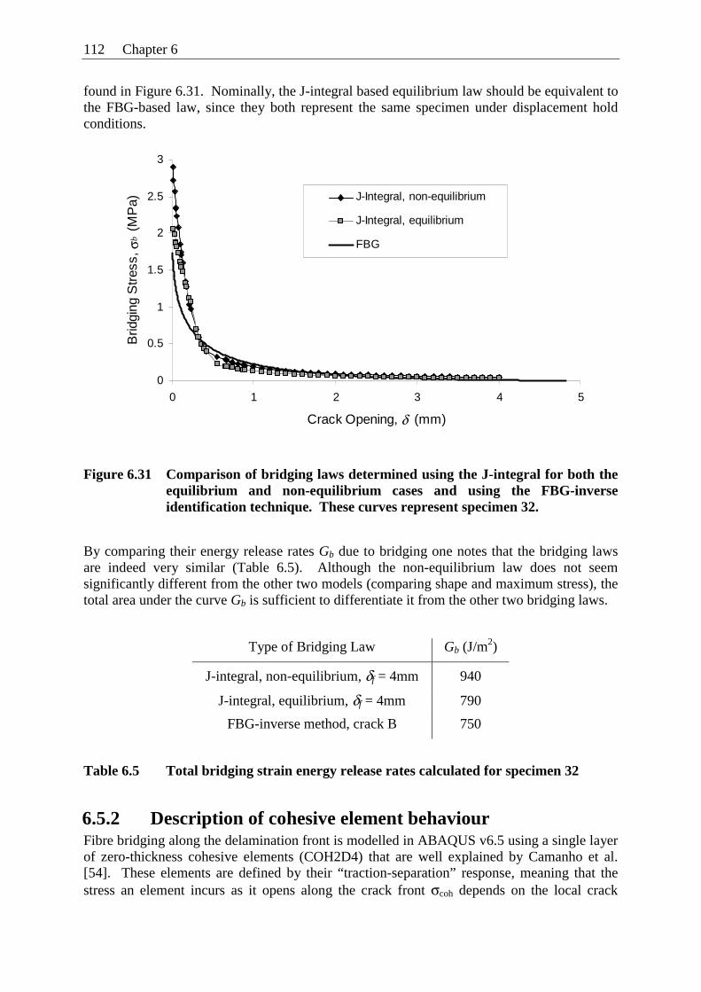
112 Chapter 6
found in Figure 6.31. Nominally, the J-integral based equilibrium law should be equivalent to the FBG-based law, since they both represent the same specimen under displacement hold conditions.
0
0.5
1
1.5
2
2.5
3
0 1 2 3 4 5
Crack Opening, δ (mm)
Brid
ging
Str
ess,
σb (
MP
a) J-Integral, non-equilibrium
J-Integral, equilibrium
FBG
Figure 6.31 Comparison of bridging laws determined using the J-integral for both the equilibrium and non-equilibrium cases and using the FBG-inverse identification technique. These curves represent specimen 32.
By comparing their energy release rates Gb due to bridging one notes that the bridging laws are indeed very similar (Table 6.5). Although the non-equilibrium law does not seem significantly different from the other two models (comparing shape and maximum stress), the total area under the curve Gb is sufficient to differentiate it from the other two bridging laws.
Type of Bridging Law Gb (J/m2)
J-integral, non-equilibrium, δf = 4mm 940
J-integral, equilibrium, δf = 4mm 790
FBG-inverse method, crack B 750
Table 6.5 Total bridging strain energy release rates calculated for specimen 32
6.5.2 Description of cohesive element behaviour Fibre bridging along the delamination front is modelled in ABAQUS v6.5 using a single layer of zero-thickness cohesive elements (COH2D4) that are well explained by Camanho et al. [54]. These elements are defined by their “traction-separation” response, meaning that the stress an element incurs as it opens along the crack front σcoh depends on the local crack
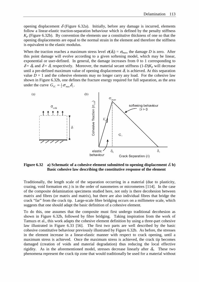
Delamination 113
opening displacement δ (Figure 6.32a). Initially, before any damage is incurred, elements follow a linear-elastic traction-separation behaviour which is defined by the penalty stiffness Kp (Figure 6.32b). By convention the elements use a constitutive thickness of one so that the opening displacements are equal to the normal strain in the element and therefore the stiffness is equivalent to the elastic modulus.
When the traction reaches a maximum stress level σ(δ0) = σmax, the damage D is zero. After this point damage will evolve according to a given softening model, which may be linear, exponential or user-defined. In general, the damage increases from 0 to 1 corresponding to δ = δ0 and δ = δ1 respectively. Moreover, the material secant stiffness (1-D)Kp will decrease until a pre-defined maximum value of opening displacement δ1 is achieved. At this separation value D = 1 and the cohesive elements may no longer carry any load. For the cohesive law shown in Figure 6.32b, one defines the fracture energy required for full separation, as the area under the curve 1max2
1 δσ=ICG .
Figure 6.32 a) Schematic of a cohesive element submitted to opening displacement δ. b) Basic cohesive law describing the constitutive response of the element
Traditionally, the length scale of the separation occurring in a material (due to plasticity, crazing, void formation etc.) is in the order of nanometres or micrometres [114]. In the case of the composite delamination specimens studied here, not only is there decohesion between matrix and fibres (or matrix and matrix), but there are also individual fibres that bridge the crack “far” from the crack tip. Large-scale fibre bridging occurs on a millimetre scale, which suggests that one should adapt the basic definition of a cohesive element.
To do this, one assumes that the composite must first undergo traditional decohesion as shown in Figure 6.32b, followed by fibre bridging. Taking inspiration from the work of Tamuzs et al., this work adapts the cohesive element definition by using a three-part cohesive law illustrated in Figure 6.33 [56]. The first two parts are well described by the basic cohesive constitutive behaviour previously illustrated by Figure 6.32b. As before, the stresses in the element increase in a linear-elastic manner with respect to crack opening, until a maximum stress is achieved. Once the maximum stress is achieved, the crack tip becomes damaged (creation of voids and material degradation) thus reducing the local effective rigidity. As in the aforementioned model, stresses decrease linearly after δ0. These two phenomena represent the crack tip zone that would traditionally be used for a material without
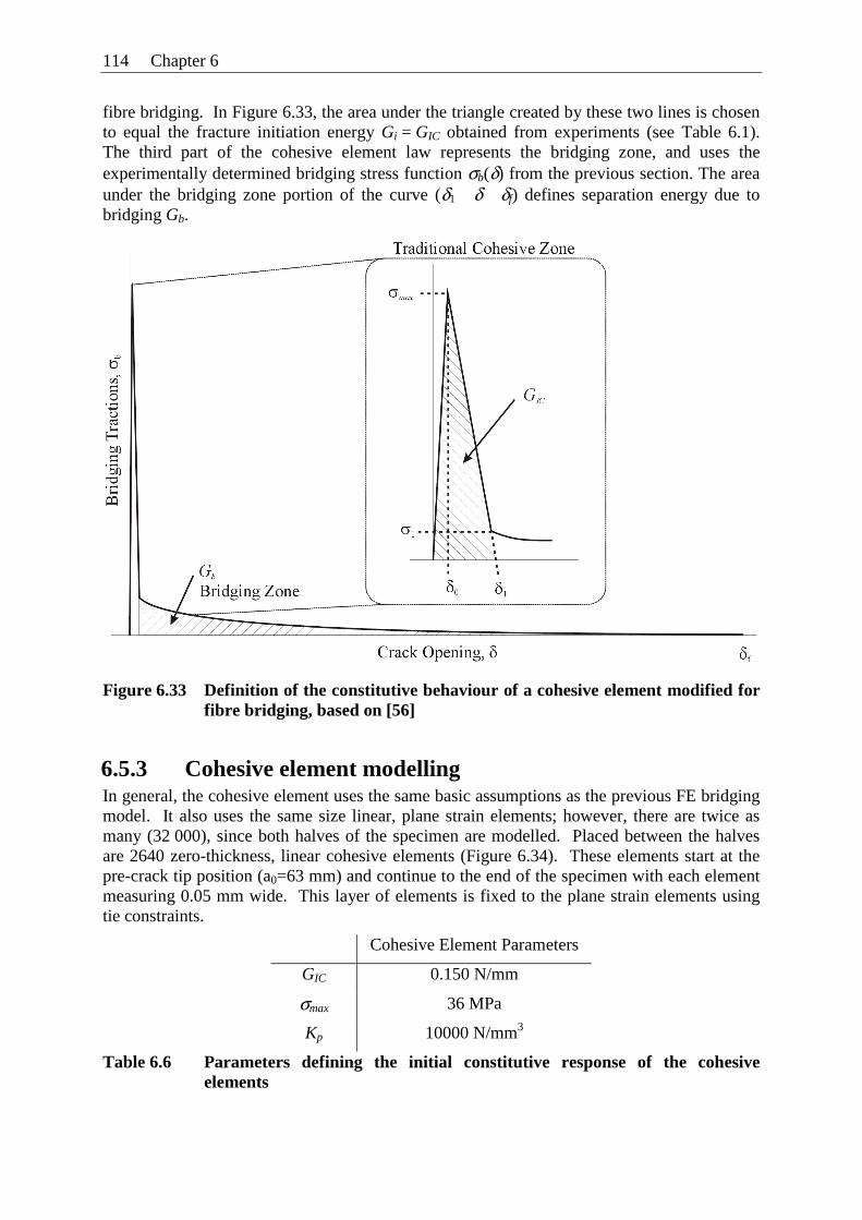
114 Chapter 6
fibre bridging. In Figure 6.33, the area under the triangle created by these two lines is chosen to equal the fracture initiation energy Gi = GIC obtained from experiments (see Table 6.1). The third part of the cohesive element law represents the bridging zone, and uses the experimentally determined bridging stress function σb(δ) from the previous section. The area under the bridging zone portion of the curve (δ1 δ δf) defines separation energy due to bridging Gb.
Figure 6.33 Definition of the constitutive behaviour of a cohesive element modified for fibre bridging, based on [56]
6.5.3 Cohesive element modelling In general, the cohesive element uses the same basic assumptions as the previous FE bridging model. It also uses the same size linear, plane strain elements; however, there are twice as many (32 000), since both halves of the specimen are modelled. Placed between the halves are 2640 zero-thickness, linear cohesive elements (Figure 6.34). These elements start at the pre-crack tip position (a0=63 mm) and continue to the end of the specimen with each element measuring 0.05 mm wide. This layer of elements is fixed to the plane strain elements using tie constraints.
Cohesive Element Parameters
GIC 0.150 N/mm
σmax 36 MPa
Kp 10000 N/mm3
Table 6.6 Parameters defining the initial constitutive response of the cohesive elements
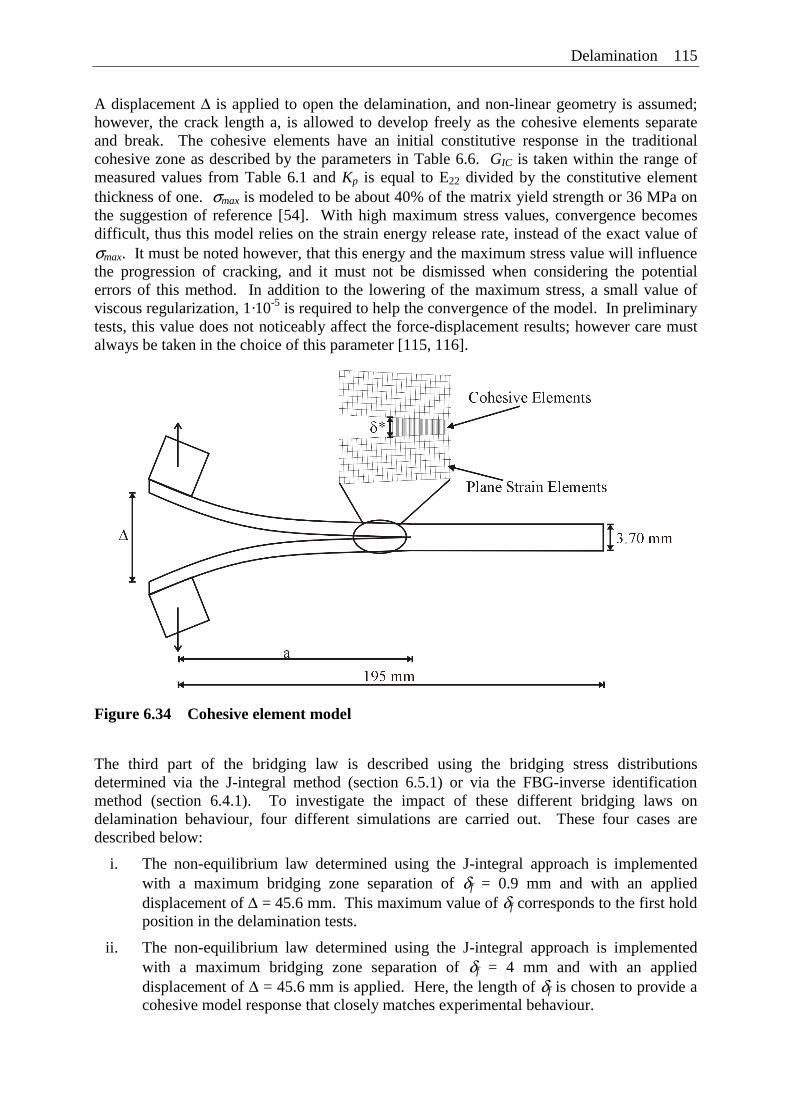
Delamination 115
A displacement Δ is applied to open the delamination, and non-linear geometry is assumed; however, the crack length a, is allowed to develop freely as the cohesive elements separate and break. The cohesive elements have an initial constitutive response in the traditional cohesive zone as described by the parameters in Table 6.6. GIC is taken within the range of measured values from Table 6.1 and Kp is equal to E22 divided by the constitutive element thickness of one. σmax is modeled to be about 40% of the matrix yield strength or 36 MPa on the suggestion of reference [54]. With high maximum stress values, convergence becomes difficult, thus this model relies on the strain energy release rate, instead of the exact value of σmax. It must be noted however, that this energy and the maximum stress value will influence the progression of cracking, and it must not be dismissed when considering the potential errors of this method. In addition to the lowering of the maximum stress, a small value of viscous regularization, 1·10-5 is required to help the convergence of the model. In preliminary tests, this value does not noticeably affect the force-displacement results; however care must always be taken in the choice of this parameter [115, 116].
Figure 6.34 Cohesive element model
The third part of the bridging law is described using the bridging stress distributions determined via the J-integral method (section 6.5.1) or via the FBG-inverse identification method (section 6.4.1). To investigate the impact of these different bridging laws on delamination behaviour, four different simulations are carried out. These four cases are described below:
i. The non-equilibrium law determined using the J-integral approach is implemented with a maximum bridging zone separation of δf = 0.9 mm and with an applied displacement of Δ = 45.6 mm. This maximum value of δf corresponds to the first hold position in the delamination tests.
ii. The non-equilibrium law determined using the J-integral approach is implemented with a maximum bridging zone separation of δf = 4 mm and with an applied displacement of Δ = 45.6 mm is applied. Here, the length of δf is chosen to provide a cohesive model response that closely matches experimental behaviour.
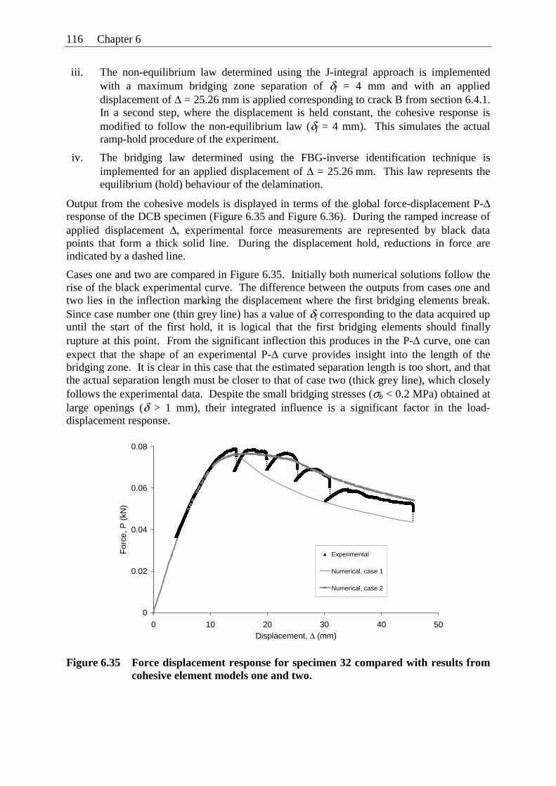
116 Chapter 6
iii. The non-equilibrium law determined using the J-integral approach is implemented with a maximum bridging zone separation of δf = 4 mm and with an applied displacement of Δ = 25.26 mm is applied corresponding to crack B from section 6.4.1. In a second step, where the displacement is held constant, the cohesive response is modified to follow the non-equilibrium law (δf = 4 mm). This simulates the actual ramp-hold procedure of the experiment.
iv. The bridging law determined using the FBG-inverse identification technique is implemented for an applied displacement of Δ = 25.26 mm. This law represents the equilibrium (hold) behaviour of the delamination.
Output from the cohesive models is displayed in terms of the global force-displacement P-Δ response of the DCB specimen (Figure 6.35 and Figure 6.36). During the ramped increase of applied displacement Δ, experimental force measurements are represented by black data points that form a thick solid line. During the displacement hold, reductions in force are indicated by a dashed line.
Cases one and two are compared in Figure 6.35. Initially both numerical solutions follow the rise of the black experimental curve. The difference between the outputs from cases one and two lies in the inflection marking the displacement where the first bridging elements break. Since case number one (thin grey line) has a value of δf corresponding to the data acquired up until the start of the first hold, it is logical that the first bridging elements should finally rupture at this point. From the significant inflection this produces in the P-Δ curve, one can expect that the shape of an experimental P-Δ curve provides insight into the length of the bridging zone. It is clear in this case that the estimated separation length is too short, and that the actual separation length must be closer to that of case two (thick grey line), which closely follows the experimental data. Despite the small bridging stresses (σb < 0.2 MPa) obtained at large openings (δ > 1 mm), their integrated influence is a significant factor in the load-displacement response.
0
0.02
0.04
0.06
0.08
0 10 20 30 40 50Displacement, Δ (mm)
For
ce, P
(kN
)
Experimental
Numerical, case 1
Numerical, case 2
Figure 6.35 Force displacement response for specimen 32 compared with results from cohesive element models one and two.
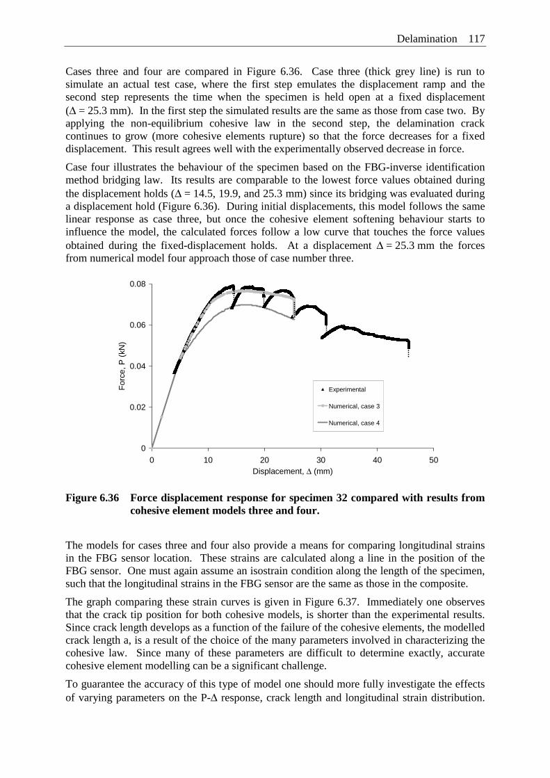
Delamination 117
Cases three and four are compared in Figure 6.36. Case three (thick grey line) is run to simulate an actual test case, where the first step emulates the displacement ramp and the second step represents the time when the specimen is held open at a fixed displacement (Δ = 25.3 mm). In the first step the simulated results are the same as those from case two. By applying the non-equilibrium cohesive law in the second step, the delamination crack continues to grow (more cohesive elements rupture) so that the force decreases for a fixed displacement. This result agrees well with the experimentally observed decrease in force.
Case four illustrates the behaviour of the specimen based on the FBG-inverse identification method bridging law. Its results are comparable to the lowest force values obtained during the displacement holds (Δ = 14.5, 19.9, and 25.3 mm) since its bridging was evaluated during a displacement hold (Figure 6.36). During initial displacements, this model follows the same linear response as case three, but once the cohesive element softening behaviour starts to influence the model, the calculated forces follow a low curve that touches the force values obtained during the fixed-displacement holds. At a displacement Δ = 25.3 mm the forces from numerical model four approach those of case number three.
0
0.02
0.04
0.06
0.08
0 10 20 30 40 50Displacement, Δ (mm)
For
ce, P
(kN
)
Experimental
Numerical, case 3
Numerical, case 4
Figure 6.36 Force displacement response for specimen 32 compared with results from cohesive element models three and four.
The models for cases three and four also provide a means for comparing longitudinal strains in the FBG sensor location. These strains are calculated along a line in the position of the FBG sensor. One must again assume an isostrain condition along the length of the specimen, such that the longitudinal strains in the FBG sensor are the same as those in the composite.
The graph comparing these strain curves is given in Figure 6.37. Immediately one observes that the crack tip position for both cohesive models, is shorter than the experimental results. Since crack length develops as a function of the failure of the cohesive elements, the modelled crack length a, is a result of the choice of the many parameters involved in characterizing the cohesive law. Since many of these parameters are difficult to determine exactly, accurate cohesive element modelling can be a significant challenge.
To guarantee the accuracy of this type of model one should more fully investigate the effects of varying parameters on the P-Δ response, crack length and longitudinal strain distribution.
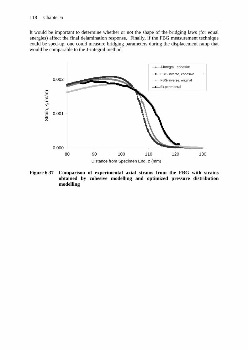
118 Chapter 6
It would be important to determine whether or not the shape of the bridging laws (for equal energies) affect the final delamination response. Finally, if the FBG measurement technique could be sped-up, one could measure bridging parameters during the displacement ramp that would be comparable to the J-integral method.
Figure 6.37 Comparison of experimental axial strains from the FBG with strains obtained by cohesive modelling and optimized pressure distribution modelling
0.000
0.001
0.002
80 90 100 110 120 130Distance from Specimen End, a+l (mm)
J-integral, cohesive
Inverse Numerical, cohesive
Inverse Numerical
Experimental
FBG-inverse, cohesive
FBG-inverse, original
Distance from Specimen End, z (mm)
Str
ain,
εz (
m/m
)
Chapter 7 Conclusions and Perspectives
The objective of this work is to develop sensing techniques based on FBG sensors in order to provide information about the non-homogeneous strain state found in CFRP composite laminates. To do this, the work focuses on two aspects causing strain in a composite material: production (residual strains) and delamination. Both cases cause non-uniform strains that are transferred from the composite to the embedded optical fibre sensor. The production strains and final residual strains in the composite reflect the anisotropy of the material and production process, which induce unequal principal strains in the FBG (εx ≠ εy ≠ εz). During delamination, a distributed strain field εz(z) develops along the length of the sensor. This must be measured in addition to the initial residual strain field.
Overall, the experiments described in this work show the excellent potential for measuring non-uniform strain fields with FBG sensors. It is possible to use these sensors to extract previously unattainable information directly from the interior of a composite structure. However, the data retrieved from an FBG should be treated with care. The challenge lays in the correct interpretation of the FBG sensor signal. This thesis work demonstrates methods for distinguishing the different components of strain affecting the sensor output so that three-dimensional, distributed measurements can be obtained. In general, the distinction of the separate components requires the introduction of polarization control to the optical measurement system.
The following paragraphs summarize the key elements of the work using FBG sensors to measure these non-uniform strain fields. The first section discusses the results of residual strain testing and modelling. The second section describes the work on delamination strain measurement and the use of this data for bridging stress law determination.
7.1 Residual strains
• Spectral shape changes and jumps in wavelength indicate transitions in the material state during the heating portion of the consolidation cycle. This includes an identification of the glass-transition temperature and the melting temperature. Key to this procedure is the monitoring of the unequal transverse strains (εx ≠ εy) that induce birefringence in the optical fibre, and thus create a split peak reflection spectrum. These are the first known measurements of material state changes in a thermoplastic composite using both traditional peak shifts and birefringence.
• As expected, due to their different coefficients of thermal expansion, the cross-ply specimens exhibit a larger residual strain accumulation than the unidirectional specimens. This is illustrated by a comparatively steep wavelength shift curve (caused by larger axial strains) during cooling.
120 Chapter 7
• The final birefringence in the FBGs embedded in cross-ply specimens is also slightly more pronounced than that in the unidirectional specimens. In unidirectional (cross-ply) specimens the average peak split is 43 pm (85 pm) which is equivalent to a transverse strain difference of 231 μm (413 μm).
• A new adaptation of the OLCR system for polarization sensitive detection allows the measurement of birefringence (unequal transverse strains) distributed along the sensor length. These measurements correspond well to spectral measurements defining peak split.
• Generalized plane strain FE models of two cases representing the residual stress and strain accumulation provide information about the influence of the mould on the accumulation of residual stresses. The two cases can be described by first, a freely dilating composite and second, a composite perfectly constrained by the steel mould lid. Models show that during cooling the strains (related to wavelengths) develop such that two models bound the experimental wavelength results. However, after removal of the mould, the experimental wavelengths see a positive wavelength jump, bringing them closer to the free, unconstrained model results. By comparing the calculated and experimental birefringence and the overall wavelength shift one concludes that the final residual stress state after demoulding is only slightly dependent on the mould contact.
• Final residual stress and strain distributions in the FBG and surrounding material are calculated using the same FE models. The unconstrained model predicts very low stresses in the unidirectional laminate, tending towards zero away from the optical fibre inclusion. For the cross-ply, modelled stresses in the 90° layer are calculated to be half the tensile strength of the PPS matrix. This may explain the tendency for micro-cracking observed in cross-ply specimens.
• In neither the unidirectional nor the cross-ply case (unconstrained) do the optical fibre inclusion case a significant detrimental stress concentration. The models also show that its disturbance of the strain and stress fields becomes negligible at a distance of approximately three fibre diameters from the FBG.
• An examination of the potential errors involved when using a simplification of the full three-dimensional optomechanical relationships is discussed. It becomes clear that loading scenarios analogous to the diametric loading test from Chapter 4 may benefit from the low sensitivity of the fast axis to transverse strains. In this way the fast axis peak can be used to estimate the residual axial strains in the cross-ply specimens. For the two cross-ply specimens these values are -310 and -380 με.
• Since the two optomechanical relationships (compensated for temperature) contain three unknown strains, a third measurement is useful for measuring the full three-dimensional strain state. A hybrid optical fibre sensing technique is demonstrated using an FBG in combination with a Fabry Perot sensor. The novelty of this method is the addition of polarization rotation to obtain birefringence information from the peak-detection system. This system thus provides the first experimental measurements of the development of all three residual strain components, even when εx ≠ εy ≠ εz. The accumulation of strains due to cooling to room temperature is shown to be 60 με along the fibre length. In the transverse directions (fast and slow axis respectively) the strains are about 40 με and -250 με.
Conclusions and Perspectives 121
7.2 Delamination
• Using the polarization adaptations to the OLCR, novel measurements of distributed axial strains εz(z) in a birefringent (induced by residual strains) FBG are obtained. This allows for the determination of the location and growth direction of delamination cracks in double cantilever beam specimens.
• Finite element models of the delamination specimen indicate that the delamination crack tip is difficult to define, which corresponds well to observations of unbroken reinforcing fibres bridging the delamination crack.
• Using the experimental wavelength distribution for comparison, it is possible to iteratively solve for parameters describing the distribution of bridging tractions across the delamination crack. This combination of FBG measurements and inverse identification via FE modelling is a novel technique for determining bridging laws from static specimens. Bridging laws determined for various specimens and crack lengths are exponential in nature with a maximum bridging stress around 1-2.5 MPa and a fibre bridging zone length of 20-50 mm depending on the delamination crack length and specimen.
• An alternate J-integral method for determining bridging laws provides a similar bridging law; however, the bridging zone length must be estimated. In cohesive element modelling the effect of this length is clearly demonstrated in the response of the force-displacement curve. Simulations predict significantly different loading responses for bridging laws measured during the applied ramp of the opening displacement compared to those during the displacement controlled hold.
• Using the FBG-inverse identification approach, the separation energy Gb due to fibre bridging is found to be 750 J/m2 for one specimen. This measurement is within 5% of the value calculated using the alternate J-integral method.
7.3 Perspectives
Given the sensitivity of an FBG sensor to the non-homogeneous strain states found in composite materials, the ultimate purpose of the sensor should be carefully considered before taking measurements. The choice of sensor length and coating may be important factors. If one only wants to measure longitudinal strains, perhaps an FBG coated in polyimide should be used to dampen transverse strain transfer to the fibre. If punctual strains are desired then a short gauge length may be better suited to the task than a long gauge sensor that will require OLCR measurement of distributed strains.
On the other hand, if one requires a full three-dimensional picture of punctual strains, a hybrid sensor like that demonstrated by Jin and Sirkis [89] may be less fragile than the EFPI tested here. The close proximity of the FBG and Fabry-Perot in the same fibre could also reduce any error due to strain gradients in the material. By combining this sensor with a means for switching the polarization angle automatically, one could retrieve all the necessary strain components.
With respect to residual strain monitoring, further investigations into the influence of the contact between the mould and the composite may interest those involved in composite production. An enhanced mechanical model including frictional contact between the mould and composite could improve the prediction of residual strains. This would of course require

122 Chapter 7
an extended investigation characterizing the contact properties between the composite, the release film and the steel mould.
Delamination measurements might benefit from the polyimide coating suggested above, to remove transverse strain effects; however, one must consider whether a third material phase or a potentially reduced sensitivity will be significant. Another means for improving delamination monitoring could be an adaptation of the OLCR for faster measurements. Alternatively a system based on an optical frequency domain reflectometer (OFDR) might be considered, since it relies on the fast sweep of a laser instead of the movement of a piezoelectric stage. In this way strain distributions could be measured in real-time as the delamination crack grows. Non-uniform strain fields like those due to impact, fatigue or vibration could also be investigated with this type of system.
Without these adaptations, the OLCR system can still provide important measurements of internal strain distributions. Measurements could be acquired to observe the influence of the distance to sensor to the delamination plane. The orientation of the sensor with respect to the crack growth direction could also be investigated. Using the method developed here, one could determine bridging laws for different composite lay-ups or fracture modes. This information could then be used to improve current predictions of crack growth progression.
References
[1] R. M. Measures, N. D. W. Glossop, J. Lymer, M. Leblanc, J. West, S. Dubois, W. Tsaw, and R. C. Tennyson, "Structurally integrated fiber optic damage assessment system for composite-materials," Applied Optics, vol. 28, pp. 2626-2633, 1989.
[2] K. O. Hill, Y. Fujii, D. C. Johnson, and B. S. Kawasaki, "Photosensitivity in optical fiber waveguides - application to reflection filter fabrication," Applied Physics Letters, vol. 32, pp. 647-649, 1978.
[3] Y. J. Rao, "Recent progress in applications of in-fibre Bragg grating sensors," Optics and Lasers in Engineering, vol. 31, pp. 297-324, 1999.
[4] D. W. Jensen, J. Pascual, and J. A. August, "Performance of graphite/bismaleimide laminates with embedded optical fibers. I. Uniaxial tension," Smart Materials and Structures, vol. 1, pp. 24-30, 1992.
[5] M. S. Kim, C. S. Lee, and W. Hwang, "Effect of the angle between optical fiber and adjacent layer on the mechanical behavior of carbon/epoxy laminates with embedded fiber-optic sensor," Journal of Materials Science Letters, vol. 19, pp. 1673-1675, 2000.
[6] D. C. Lee, J. J. Lee, and S. J. Yun, "The mechanical characteristics of smart composite structures with embedded optical-fiber sensors," Composite Structures, vol. 32, pp. 39-50, 1995.
[7] D. W. Jensen, J. Pascual, and J. A. August, "Performance of graphite/bismaleimide laminates with embedded optical fibers. II. Uniaxial compression," Smart Materials and Structures, vol. 1, pp. 31, 1992.
[8] M. Surgeon and M. Wevers, "Static and dynamic testing of a quasi-isotropic composite with embedded optical fibres," Composites Part A-Applied Science and Manufacturing, vol. 30, pp. 317-324, 1999.
[9] A. Skontorp, "Structural integrity of quasi-isotropic composite laminates with embedded optical fibers," Journal of Reinforced Plastics and Composites, vol. 19, pp. 1056-1077, 2000.
[10] R. A. Badcock and G. F. Fernando, "Intensity-based optical fibre sensor for fatigue damage detection in advanced fibre-reinforced composites," Smart Materials and Structures, vol. 4, pp. 223-230, 1995.
124 References
[11] J. A. Nairn and P. Zoller, "Matrix solidification and the resulting residual thermal-stresses in composites," Journal of Materials Science, vol. 20, pp. 355-367, 1985.
[12] B. J. Weteringe, H. E. N. Bersee, and A. Beukers, "Characterization of microcracking in PPS laminates," presented at 23rd International European Chapter SAMPE Conference, Paris, pp. 225-236, 2002.
[13] J. A. Barnes and G. E. Byerly, "The formation of residual-stresses in laminated thermoplastic composites," Composites Science and Technology, vol. 51, pp. 479-494, 1994.
[14] Y. K. Kim and I. M. Daniel, "Cure cycle effect on composite structures manufactured by resin transfer molding," Journal of Composite Materials, vol. 36, pp. 1725-1743, 2002.
[15] W. J. Unger and J. S. Hansen, "The effect of thermal-processing on residual strain development in unidirectional graphite fiber reinforced PEEK," Journal of Composite Materials, vol. 27, pp. 59-82, 1993.
[16] G. Jeronimidis and A. T. Parkyn, "Residual-stresses in carbon fiber-thermoplastic matrix laminates," Journal of Composite Materials, vol. 22, pp. 401-415, 1988.
[17] N. Ersoy and O. Vardar, "Measurement of residual stresses in layered composites by compliance method," Journal of Composite Materials, vol. 34, pp. 575-598, 2000.
[18] J. A. E. Manson and J. C. Seferis, "Process Simulated Laminate (PSL) - a methodology to internal-stress characterization in advanced composite-materials," Journal of Composite Materials, vol. 26, pp. 405-431, 1992.
[19] A. P. Deshpande and J. C. Seferis, "Processing characteristics in different semi-crystalline thermoplastic composites using process simulated laminate (PSL) methodology," Journal of Thermoplastic Composite Materials, vol. 9, pp. 183-198, 1996.
[20] O. Sicot, X. L. Gong, A. Cherouat, and J. Lu, "Determination of residual stress in composite laminates using the incremental hole-drilling method," Journal of Composite Materials, vol. 37, pp. 831-844, 2003.
[21] G. B. Chai, H. K. Chin, H. M. Xie, and A. Asundi, "Residual interlaminar deformation analysis in the carbon/epoxy composites using micro-moire interferometry," Composites Science and Technology, vol. 63, pp. 171-175, 2003.
[22] M. C. Li, J. J. Wu, A. C. Loos, and J. Morton, "Plane-strain finite element model for process-induced residual stresses in a graphite/PEEK composite," Journal of Composite Materials, vol. 31, pp. 212-243, 1997.
References 125
[23] C. Filiou, C. Galiotis, and D. N. Batchelder, "Residual-stress distribution in carbon-fiber thermoplastic matrix preimpregnated composite tapes," Composites, vol. 23, pp. 28-38, 1992.
[24] R. Meske and E. Schnack, "Particular adaptation of X-ray diffraction to fiber reinforced composites," Mechanics of Materials, vol. 35, pp. 19-34, 2003.
[25] F. Colpo, L. Humbert, P. Giaccari, and J. Botsis, "Characterization of residual strains in an epoxy block using an embedded FBG sensor and the OLCR technique," Composites Part A: Applied Science and Manufacturing, vol. 37, pp. 652-661, 2006.
[26] V. Dewynter-Marty, P. Ferdinand, E. Bocherens, R. Carbone, H. Beranger, S. Bourasseau, M. Dupont, and D. Balageas, "Embedded Fiber Bragg Grating sensors for industrial composite cure monitoring," Journal of Intelligent Material Systems and Structures, vol. 9, pp. 785-787, 1998.
[27] C. M. Lawrence, D. V. Nelson, J. R. Spingarn, and T. E. Bennett, "Measurement of process-induced strains in composite materials using embedded fiber optic sensors," presented at Smart Structures and Materials 1996: Smart Sensing, Processing, and Instrumentation, San Diego, CA, pp. 60-68, 1996.
[28] J. M. Menendez and J. A. Guemes, "Bragg grating-based multiaxial strain sensing: its application to residual strain measurement in composite laminates," presented at Smart Structures and Materials 2000: Sensory Phenomena and Measurement Instrumentation for Smart Structures and Materials, Newport Beach, CA, USA, pp. 271-281, 2000.
[29] J. A. Güemes, M. Frovel, Rodriguez-Lence, and J. M. Menendez, "Embedded fiber Bragg grating as local damage sensors for composite materials," in Smart Structures and Materials 2002: Smart Sensor Technology and Measurement Systems, vol. 4694, D. Inaudi and E. Udd, Eds. San Diego: SPIE, 2002, pp. 118-128.
[30] Y. Okabe, S. Yashiro, R. Tsuji, T. Mizutani, and N. Takeda, "Effect of thermal residual stress on the reflection spectrum from fiber Bragg grating sensors embedded in CFRP laminates," Composites Part A-Applied Science and Manufacturing, vol. 33, pp. 991-999, 2002.
[31] K. S. C. Kuang, R. Kenny, M. P. Whelan, W. J. Cantwell, and P. R. Chalker, "Residual strain measurement and impact response of optical fibre Bragg grating sensors in fibre metal laminates," Smart Materials and Structures, vol. 10, pp. 338-346, 2001.
[32] K. S. C. Kuang, R. Kenny, M. P. Whelan, W. J. Cantwell, and P. R. Chalker, "Embedded fibre Bragg grating sensors in advanced composite materials," Composites Science and Technology, vol. 61, pp. 1379-1387, 2001.
[33] K. S. C. Kuang, L. Zhang, W. J. Cantwell, and I. Bennion, "Process monitoring of aluminum-foam sandwich structures based on thermoplastic fibre-metal laminates
126 References
using fibre Bragg gratings," Composites Science and Technology, vol. 65, pp. 669-676, 2005.
[34] L. P. Kollár and G. S. Springer, Mechanics of composite structures. Cambridge: Cambridge University Press, 2003.
[35] C. Wang and C. T. Sun, "Experimental characterization of constitutive models for PEEK thermoplastic composite at heating stage during forming," Journal of Composite Materials, vol. 31, pp. 1480-506, 1997.
[36] A. Johnston, R. Vaziri, and A. Poursartip, "A plane strain model for process-induced deformation of laminated composite structures," Journal of Composite Materials, vol. 35, pp. 1435-1469, 2001.
[37] F. O. Sonmez and E. Eyol, "Optimal post-manufacturing cooling paths for thermoplastic composites," Composites Part A: Applied Science and Manufacturing, vol. 33, pp. 301-314, 2002.
[38] T. J. Chapman, J. W. Gillespie, R. B. Pipes, J. A. E. Manson, and J. C. Seferis, "Prediction of Process-Induced Residual-Stresses in Thermoplastic Composites," Journal of Composite Materials, vol. 24, pp. 616-643, 1990.
[39] P. Sunderland, W. J. Yu, and J. A. Manson, "A thermoviscoelastic analysis of process-induced internal stresses in thermoplastic matrix composites," Polymer Composites, vol. 22, pp. 579-592, 2001.
[40] B. S. Kim, N. Bernet, P. Sunderland, and J. A. Manson, "Numerical analysis of the dimensional stability of thermoplastic composites using a thermoviscoelastic approach," Journal of Composite Materials, vol. 36, pp. 2389-2403, 2002.
[41] Y. Bar-Cohen, "Emerging NDE technologies and challenges at the beginning of the 3rd millennium – part I," NDTnet, vol. 5, 2000.
[42] T. Lüthi, Non-destructive evaluation methods (course notes): EMPA, 2004.
[43] C. C. Tsao and H. Hocheng, "Computerized tomography and C-Scan for measuring delamination in the drilling of composite materials using various drills," International Journal of Machine Tools & Manufacture, vol. 45, pp. 1282-1287, 2005.
[44] N. P. Avdelidis, D. P. Almond, A. Dobbinson, B. C. Hawtin, C. Ibarra-Castanedo, and X. Maldague, "Aircraft composites assessment by means of transient thermal NDT," Progress in Aerospace Sciences, vol. 40, pp. 143-162, 2004.
[45] M. L. Benzeggagh, Y. Prel, and F. X. Charentenay, "Experimental analysis of mode I delamination testing," presented at Fifth International Conference on Composite Materials ICCM-V, San Diego, California, pp. 127-139, 1985.
References 127
[46] Y. Zou, L. Tong, and G. P. Steven, "Vibration-based model-dependent damage (delamination) identification and health monitoring for composite structures - A review," Journal of Sound and Vibration, vol. 230, pp. 357-378, 2000.
[47] J. S. Leng and A. Asundi, "Non-destructive evaluation of smart materials by using extrinsic Fabry-Perot interferometric and fiber Bragg grating sensors," NDT & E International, vol. 35, pp. 273-276, 2002.
[48] T. S. P. Austin, M. M. Singh, P. J. Gregson, J. P. Dakin, and P. M. Powell, "Damage assessment in hybrid laminates using an array of embedded fibre optic sensors," in 1999 Smart Structures and Materials Smart Systems for Bridges, Structures, and Highways, vol. 3671, Proceedings-of-SPIE-The-International-Society-for-Optical-Engineering. Newport Beach, CA: SPIE, 1999, pp. 281-288.
[49] N. Takeda, Y. Okabe, R. Tsuji, and I. Takeda Shin, "Application of chirped fiber Bragg grating sensors for damage identification in composites," in Smart Structures and Materials 2002 Smart Sensor Technology and Measurement Systems, vol. 4694, Proceedings-of-SPIE-The-International-Society-for-Optical-Engineering, D. Inaudi and E. Udd, Eds. San Diego, CA, United States: SPIE, 2002, pp. 106-117.
[50] H. Y. Ling, K. T. Lau, L. Cheng, and W. Jin, "Utilization of embedded optical fibre sensors for delamination characterization in composite laminates using a static strain method," Smart Materials & Structures, vol. 14, pp. 1377-1386, 2005.
[51] S. Takeda, S. Minakuchi, Y. Okabe, and N. Takeda, "Delamination monitoring of laminated composites subjected to low-velocity impact using small-diameter FBG sensors," Composites Part a-Applied Science and Manufacturing, vol. 36, pp. 903-908, 2005.
[52] S. Takeda, Y. Okabe, and N. Takeda, "Delamination detection in CFRP laminates with embedded small-diameter fiber Bragg grating sensors," Composites Part A-Applied Science and Manufacturing, vol. 33, pp. 971-980, 2002.
[53] T. L. Anderson, Fracture mechanics fundamentals and applications, Second ed. Boca Raton etc . CRC Press, 1995.
[54] P. P. Camanho, C. G. Dávila, and D. R. Ambur, "Numerical simulation of delamination growth in composite materials," NASA Langley Research Center, Hampton, NASA/TP-2001-211041, 2001.
[55] R. de Borst and J. J. C. Remmers, "Computational modelling of delamination," Composites Science and Technology, vol. 66, pp. 713-722, 2006.
[56] V. Tamuzs, S. Tarasovs, and U. Vilks, "Progressive delamination and fiber bridging modeling in double cantilever beam composite specimens," Engineering Fracture Mechanics, vol. 68, pp. 513-525, 2001.
128 References
[57] G. Alfano and M. A. Crisfield, "Finite element interface models for the delamination analysis of laminated composites: mechanical and computational issues," International Journal for Numerical Methods in Engineering, vol. 50, pp. 1701-1736, 2001.
[58] F. Zok and C. L. Hom, "Large-scale bridging in brittle matrix composites," Acta Metallurgica Et Materialia, vol. 38, pp. 1895-&, 1990.
[59] G. I. Barenblatt, "The mathematical theory of equilibrium cracks in brittle fracture," Advances in Applied Mechanics, vol. 7, pp. 55-129 30-48??, 1962.
[60] D. S. Dugdale, "Yielding of Steel Sheets Containing Slits," Journal of the Mechanics and Physics of Solids, vol. 8, pp. 100-104, 1960.
[61] A. Hillerborg, M. Modéer, and P.-E. Petersson, "Analysis of crack formation and crack growth in concrete by means of fracture mechanics and finite elements," Cement and Concrete Research, vol. 6, pp. 773-781, 1976.
[62] M. A. Crisfield, H. B. Hellweg, and G. A. O. Davies, "Failure analysis of compoiste structures using interface elements," presented at NAFEMS conference on application of finite elements to composite materials, London, UK, 1997.
[63] B. F. Sorensen and T. K. Jacobsen, "Determination of cohesive laws by the J integral approach," Engineering Fracture Mechanics, vol. 70, pp. 1841-1858, 2003.
[64] J. R. Rice, "Path independent integral and approximate analysis of strain concentration by notches and cracks," Journal of Applied Mechanics, vol. 379-386, 1968.
[65] P. Giaccari, G. R. Dunkel, L. Humbert, J. Botsis, H. G. Limberger, and R. P. Salathe, "On a direct determination of non-uniform internal strain fields using fibre Bragg gratings," Smart Materials & Structures, vol. 14, pp. 127-136, 2005.
[66] A. W. Snyder and J. D. Love, Optical waveguide theory. London New York: Chapman & Hall, 1983.
[67] L. B. Jeunhomme, Single-mode fiber optics principles and applications, Second ed. New York etc.: Dekker, 1990.
[68] K. O. Hill and G. Meltz, "Fiber Bragg grating technology fundamentals and overview," Lightwave Technology, Journal of, vol. 15, pp. 1263-1276, 1997.
[69] J. Skaar and O. H. Waagaard, "Design and characterization of finite-length fiber gratings," IEEE Journal of Quantum Electronics, vol. 39, pp. 1238-1245, 2003.
References 129
[70] P. Giaccari, "Fiber Bragg grating characterization by optical low coherence reflectometry and sensing applications," PhD Thesis, Ecole polytechnique fédérale de Lausanne, Lausanne, 2003.
[71] T. Erdogan, "Fiber grating spectra," Journal of Lightwave Technology, vol. 15, pp. 1277-1294, 1997.
[72] J. S. Sirkis, "Unified approach to phase-strain-temperature models for smart structure interferometric optical fiber sensors: part 1, development," Optical Engineering, vol. 32, pp. 752-761, 1993.
[73] R. J. Van Steenkiste and G. S. Springer, Strain and temperature measurement with fiber optic sensors. Lancaster: Technomic Publishing, 1997.
[74] C. D. Butter and G. B. Hocker, "Fiber optics strain-gauge," Applied Optics, vol. 17, pp. 2867-2869, 1978.
[75] M. Studer, K. Peters, and J. Botsis, "Method for determination of crack bridging parameters using long optical fiber Bragg grating sensors," Composites Part B-Engineering, vol. 34, pp. 347-359, 2003.
[76] Y. Okabe, S. Yashiro, T. Kosaka, and N. Takeda, "Detection of transverse cracks in CFRP composites using embedded fiber Bragg grating sensors," Smart Materials & Structures, vol. 9, pp. 832-838, 2000.
[77] M. M. Ohn, S. Sandgren, S. H. Huang, R. Maaskant, R. Stubbe, B. Sahlgren, R. M. Measures, and H. Storoey, "Phase-based Bragg intra-grating sensing of strain gradients," presented at Smart Structures and Materials 1995: Smart Sensing, Processing, and Instrumentation, San Diego, CA, pp. 127-135, 1995.
[78] J. S. Sirkis, "Unified approach to phase-strain-temperature models for smart structure interferometric optical fiber sensors: part 2, applications," Optical Engineering, vol. 32, pp. 762-773, 1993.
[79] R. B. Wagreich and J. S. Sirkis, "Distinguishing Fiber Bragg Grating Strain Effects," presented at 12th International Conference on Optical Fiber Sensors, Williamsburg, VA, pp. 20-23, 1997.
[80] M. Yamada and K. Sakuda, "Analysis of almost-periodic distributed feedback slab waveguides via a fundamental matrix approach," Applied Optics, vol. 26, pp. 3474-3478, 1987.
[81] M. Prabhugoud and K. Peters, "Modified transfer matrix formulation for Bragg grating strain sensors," Journal of Lightwave Technology, vol. 22, pp. 2302-2309, 2004.
130 References
[82] K. Peters, P. Pattis, J. Botsis, and P. Giaccari, "Experimental verification of response of embedded optical fiber Bragg grating sensors in non-homogeneous strain fields," Optics and Lasers in Engineering, vol. 33, pp. 107-119, 2000.
[83] H. J. Patrick, G. M. Williams, A. D. Kersey, J. R. Pedrazzani, and A. M. Vengsarkar, "Hybrid fiber Bragg grating/long period fiber grating sensor for strain/temperature discrimination," IEEE Photonics Technology Letters, vol. 8:, pp. 1223-1225, 1996.
[84] M. G. Xu, J. L. Archambault, L. Reekie, and J. P. Dakin, "Discrimination between strain and temperature effects using dual-wavelength fibre grating sensors," Electronics Letters, vol. 30, pp. 1085-1087, 1994.
[85] S. W. Case, J. J. Lesko, B. R. Fogg, and G. P. Carman, "Embedded Extrinsic Fabry-Perot Fiber Optic Strain Rosette Sensors," Journal of Intelligent Material Systems and Structures, vol. 5, pp. 412-417, 1994.
[86] S. Magne, S. Rougeault, M. Vilela, and P. Ferdinand, "State-of-strain evaluation with fiber Bragg grating rosettes: application to discrimination between strain and temperature effects in fiber sensors," Applied Optics, vol. 36, pp. 9437-9447, 1997.
[87] E. Udd, W. Schulz, J. Seim, G. McGill, and H. M. Laylor, "Distributed Multiaxis Fiber Grating Strain Sensor Applications for Bridges," in Fiber Optic Sensors for Construction Materials and Bridges. Pennsylvania: Technomic, 1998, pp. 168-180.
[88] E. Udd, C. M. Lawrence, and D. V. Nelson, "Development of a three-axis strain and temperature fiber optic grating sensor," presented at Smart Structures and Materials 1997: Smart Sensing, Processing, and Instrumentation, SPIE Vol. 3042, pp. 229-236, 1997.
[89] X. D. Jin, J. S. Sirkis, J. K. Chung, and V. S. Venkat, "Simultaneous measurement of two strain components in composite structures using embedded fiber sensor," Journal of Composite Materials, vol. 33, pp. 1376-1389, 1999.
[90] V. Bhatia, K. A. Murphy, R. O. Claus, T. A. Tran, and J. A. Greene, "Recent developments in optical-fiber-based extrinsic Fabry-Perot interferometric strain sensing technology," Smart Materials & Structures, vol. 4, pp. 246-251, 1995.
[91] G. P. Agrawal, Fiber-optic communication systems, 3rd ed. New York: Wiley-Interscience, 2002.
[92] L. Williams, "Quality assurance test method for laminate preparation in a one press process," Cytec Fiberite Inc. MP-128, Rev. A, March 13 1991.
[93] O. Comte, "Délamination d'un materiau composite avec integration d'un reseau de Bragg," Laboratoire de mécanique appliquée et d'analyse de fiabilité, Diploma Thesis, Ecole polytechnique fédérale de Lausanne, 2005.
References 131
[94] F. L. Matthews and R. D. Rawlings, Composite materials: engineering and science. London etc.: Chapman & Hall, 1994.
[95] J. Cugnoni, "Identification par recalage modal et fréquentiel des propriétés constitutives de coques en matériaux composites," PhD Thesis, Ecole polytechnique fédérale de Lausanne, Lausanne, pp. 248, 2005.
[96] D. Leach, (Cytec Industries Inc.) private communication with L. Sorensen on Aug. 1, 2003.
[97] Ticona, "Fortron 0214 - Data Sheet," Ticona (Cleanese AG) 2000.
[98] R. W. Hertzberg, Deformation and fracture mechanics of engineering materials, Fourth ed. New York etc.: Wiley, 1996.
[99] M. Douay, E. Fertein, W. X. Xie, P. Bernage, P. Niay, J. F. Bayon, and T. Georges, "Thermal hysteresis of Bragg wavelengths of intra-core fiber gratings," IEEE Photonics Technology Letters, vol. 5, pp. 1331-1334, 1993.
[100] R. B. Wagreich, W. A. Atia, H. Singh, and J. S. Sirkis, "Effects of diametric load on fibre Bragg gratings fabricated in low birefringent fibre," Electronics Letters, vol. 32, pp. 1223-1224, 1996.
[101] S. P. Timoshenko and J. N. Goodier, Theory of elasticity, Third ed. New York: McGraw-Hill Book Company, 1970.
[102] A. Bertholds and R. Dandliker, "Determination of the individual strain-optic coefficients in single-mode optical fibres," Journal of Lightwave Technology, vol. 6, pp. 17-20, 1988.
[103] J. Jang and S. Kim Hak, "Performance improvement of glass fiber-poly(phenylene sulfide) composite," Journal of Applied Polymer Science, vol. 60, pp. 2297-2306, 1996.
[104] N. Amoudruz, "Mesure des contraintes résiduelles au sein d'un matériau composite en carbone," Laboratoire de mécanique appliquée et d'analyse de fiabilité, Diploma Thesis, Ecole polytechnique fédérale de Lausanne, 2005.
[105] M. Facchini, J. Botsis, and L. Sorensen, "Measurements of temperature during fatigue of a thermoplastic polymer composite using FBG sensors," submitted to Smart Structures and Materials.
[106] A. B. Pereira and A. B. de Morais, "Mode I interlaminar fracture of carbon/epoxy multidirectional laminates," Composites Science and Technology, vol. 64, pp. 2261-2270, 2004.
132 References
[107] P. Davies, M. L. Benzeggagh, and F. X. de Charentenay, "Delamination behavior of carbon fiber reinforced PPS," presented at 32nd International SAMPE Symposium and Exhibition: Advanced Materials Technology '87, Covina, CA, USA, pp. 134-146, 1987.
[108] C. C. M. Ma, J. E. O'Connor, and A. Y. Lou, "Polyphenylene sulfide high performance composites," SAMPE Quarterly, vol. 15, pp. 12-17, 1984.
[109] J. E. O'Connor, A. Y. Lou, and W. H. Beever, "Polyphenylene sulfide - a thermoplastic polymer matrix for high performance composites," presented at The 5th International Conference on Composite Materials (ICCM-5), San Diego, pp. 963-970, 1985.
[110] "Corning SMF-28e Optical Fiber Product Information," January 2005.
[111] The MathWorks Inc., lsqnonlin (Optimization Toolbox): Version 7.0.4.365, Release 14, January 2005.
[112] Z. Suo, G. Bao, and B. Fan, "Delamination R-curve phenomena due to damage," Journal of the Mechanics and Physics of Solids, vol. 40, pp. 1-16, 1992.
[113] A. Szekrenyes and J. Uj, "Advanced beam model for fiber-bridging in unidirectional composite double-cantilever beam specimens," Engineering Fracture Mechanics, vol. 72, pp. 2686-2702, 2005.
[114] N. Chandra, H. Li, C. Shet, and H. Ghonem, "Some issues in the application of cohesive zone models for metal-ceramic interfaces," International Journal of Solids and Structures, vol. 39, pp. 2827-2855, 2002.
[115] Hibbitt, Karlsson, and Sorensen, ABAQUS benchmarks manual , Version 6.5: ABAQUS, Inc., 2004.
[116] Hibbitt, Karlsson, and Sorensen, ABAQUS example problems manual, Version 6.5: ABAQUS, Inc., 2004.

Appendix A – Silane Preparation
To prepare glass fibres for better adhesion in polyphenylene sulphide, a silane treatment is prepared as follows. By weight add:
• 1% Silquest RC-2 silane (black tar-like substance)
• 1.5% distilled water
• 97.5% alcohol (ethanol)
1. Mix silane solution for 1 hour
2. Place clean fibre (preferably just after sulphuric acid removal of the coating) in solution for 10 minute
3. Rinse fibre with alcohol.
4. Dry in oven for a minimum time and temperature of 120°C and 45 minutes.
5. Keep dry and use within 24 hours.
Be careful to avoid mechanical contact with the bare fibre as it can degrade its strength.


Larissa K. Sorensen
Bruchstrasse 12 Canadian 6003 Luzern Married [email protected] Date of Birth: 20.07.1975
Education 2003-2006 Doctoral Candidate in Mechanical Engineering, “The response of embedded FBG sensors to
non-uniform strains in CFRP composites during processing and delamination”, Ecole Polytechnique Fédérale de Lausanne (EPFL), Switzerland • Courses in Fracture Mechanics, Extended Finite Element Method and Non-destructive Testing
1999-2002 Master of Applied Science, Mechanical Engineering, “Cyclic Damage Evolution in 45° Off-
Axis Carbon Fibre-Reinforced Epoxy Composite”, University of Waterloo, Canada • Ontario Graduate Scholarship in Science and Technology • Courses in Advanced Engineering Fatigue Design and Non-Metallic Materials
1994-1999 Bachelor of Applied Science, Mechanical Engineering, University of Waterloo, Canada
• George Dufault Medal for Excellence in Communication • Procter and Gamble, Outstanding Work Report Award • Courses in Fatigue and Fracture, Finite Element Methods and Industrial Metallurgy
Professional Experience 2003-2006 Research/Teaching Assistant, EPFL, Lausanne Switzerland
• Design and perform tests on composite materials using fibre optic sensors to detect strains during processing and during delamination damage
• Finite element analysis of residual stresses and delamination • Supervise picosatellite “SwissCube” structural design and configuration team • Supervised two Master theses and seven semester projects
1999-2002 Research/Teaching Assistant, University of Waterloo, Waterloo, Canada
• Designed and implemented fatigue tests including: grip design, data acquisition, strain gauging • Taught tutorials and developed laboratory experiments for courses in Solid Mechanics,
Metallurgy and Materials Science • Mechanical Engineering Department Teaching Assistant Award
1998 Failure Analysis Engineering (4 month internship), Quality Engineering Test
Establishment, Department of National Defence, Hull, Canada • Managed projects, and wrote evaluations and recommendations for failed components • Evaluated parts for material conformance using destructive and non-destructive techniques • Analysed fractures using scanning electron microscopy and energy dispersive x-ray technique • Calculated loading scenarios, including fatigue
1997 Research Engineering (8 month internship), University of Waterloo, Waterloo, Canada
• Managed a research project investigating stress corrosion cracking in pipeline steel • Designed and built stress corrosion cracking test apparatus • Performed crack-face analysis using scanning electron microscopy • Prepared test specimens, including fatigue crack initiation, potential drop wiring and
electrochemical connections

Larissa K. Sorensen 1995-1996 Quality/Project Engineering (8 month internship), Manchester Plastics Ltd. Ontario, Canada
• Developed network databases in Lotus Notes Groupware • Wrote procedures, flow charts and work instructions to meet QS9000 (equiv. ISO9000) • Trained co-workers in the use of databases and new QS9000 procedures • Coordinated mould tests and movements, prototype shipments, vendor quotations, etc.
1995 Research & Development (4 month internship), IPSCO Inc., Regina, Canada
• Performed steel structure, strength and composition analysis using: tensile tests, scanning electron microscopy, energy dispersive x-ray technique, computer-aided image analysis, microscopes and hardness testers
• Prepared steel samples for microscopic analysis
Awards 2006 Special Mention for Poster Presentation, 6th EUROMECH Solid Mechanics Conference 2000-2001 University of Waterloo Graduate Scholarships, University of Waterloo 2001 Mechanical Engineering Department Teaching Assistant Award, University of Waterloo 2001 Ontario Graduate Scholarship in Science and Technology, administered by the University of
Waterloo 2001 Faculty of Engineering Graduate Scholarship, University of Waterloo 1999 George Dufault Medal for Excellence in Communication, University of Waterloo 1999 Ontario Engineering Competition, Explanatory Communications, 1st Place Prize 1999 Canadian Engineering Competition, Explanatory Communications, 2nd Place Prize 1994-1999 Canada Scholarship, University of Waterloo for the Government of Canada 1998 Procter and Gamble, Outstanding Work Report Award, University of Waterloo 1998 Sir Sanford Flemming Technical Presentation, 1st Place Prize, University of Waterloo 1994 Association of Professional Engineers of Ontario Entrance Scholarship, University of Waterloo
Publications and Presentations
• M. Facchini, L. Sorensen, and J. Botsis, Measurements of temperature during fatigue of a thermoplastic polymer composite using FBG sensors (submitted to Smart Materials and Structures)
• L. Sorensen, T. Gmür and J. Botsis, Residual strain development in an AS4/PPS thermoplastic composite measured using fibre Bragg grating sensors (Comp. Part A, 37, 2006, p270-281)
• L. Sorensen, T. Gmür and J. Botsis, Investigation of residual strains and delamination in AS4/PPS composite using Fibre Bragg Grating sensors (presented at the 6th EUROMECH Solid Mechanics Conference, Budapest, 2006)
• L. Sorensen, T. Gmür and J. Botsis, Delamination propagation measurement in AS4/PPS using long gauge-length FBG sensors (presented at CompTest 2006, Porto, 2006)
• L. Sorensen, T. Gmür and J. Botsis, Long FBG sensor characterization of residual strains in AS4/PPS thermoplastic laminates (SPIE vol. 5384, 2004, p267-278)
• L. Sorensen and A. Plumtree, Assessment of Matrix Damage in a Carbon-Epoxy Laminate under Cyclic Loading (ASTM STP 1435, 2003, p336-348)
Activities and Memberships
• Scout and Girl Guide Leader (1999-present) • Swiss Alpine Club (2005-present) • University Choirs, Waterloo and Lausanne (1999-2005) • Student pilot at Guelph Gliding and Soaring Association (2000-2002) • Canadian Aeronautics and Space Institute member (1997-2002)