The Rice World Gas Trade Model (RWGTM)

The Rice World Gas Trade Model (RWGTM): Report of Reference Case Results

prepared by:

Kenneth B Medlock III James A Baker III and Susan G Baker Fellow in Energy and Resource Economics, and

Deputy Director, Energy Forum, James A Baker III Institute for Public Policy Adjunct Professor, Department of Economics

Rice University

May 9, 2012

James A Baker III Institute for Public Policy Rice University 1

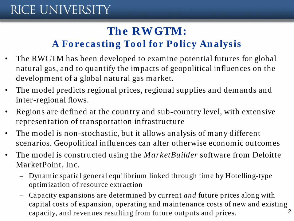
The RWGTM: A Forecasting Tool for Policy Analysis

• The RWGTM has been developed to examine potential futures for global natural gas, and to quantify the impacts of geopolitical influences on the development of a global natural gas market.

• The model predicts regional prices, regional supplies and demands and inter-regional flows.

• Regions are defined at the country and sub-country level, with extensive representation of transportation infrastructure

• The model is non-stochastic, but it allows analysis of many different scenarios. Geopolitical influences can alter otherwise economic outcomes

• The model is constructed using the MarketBuilder software from Deloitte MarketPoint, Inc.

– Dynamic spatial general equilibrium linked through time by Hotelling-type optimization of resource extraction

– Capacity expansions are determined by current and future prices along with capital costs of expansion, operating and maintenance costs of new and existing capacity, and revenues resulting from future outputs and prices. 2

Demand

3

The RWGTM: Demand

• Recall, there are over 290 regions – Regional detail is dependent on data availability and

existing infrastructure.

– In US, sub-state detail is substantial and is based on data from the Economic Census and the location of power plants.

• For example, 10 regions in Texas, 4 regions in Louisiana, 3 regions in Massachusetts, 4 regions in California, etc.

– In Rest of World, sub-national detail varies based on infrastructure and data availability.

• For example, 5 regions in India, 7 regions in China, 6 regions in Germany, 4 regions in the UK, 6 regions in France, 10 regions in Australia, 1 region in Bangladesh, 1 region in Thailand, etc.

4

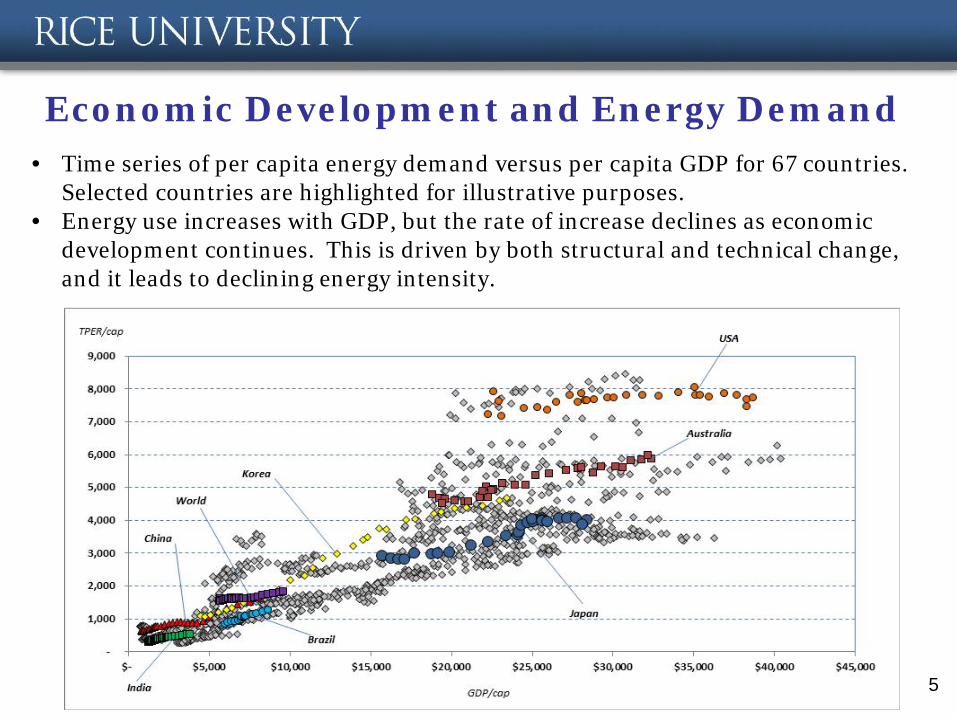
Economic Development and Energy Demand

5

• Time series of per capita energy demand versus per capita GDP for 67 countries. Selected countries are highlighted for illustrative purposes.

• Energy use increases with GDP, but the rate of increase declines as economic development continues. This is driven by both structural and technical change, and it leads to declining energy intensity.

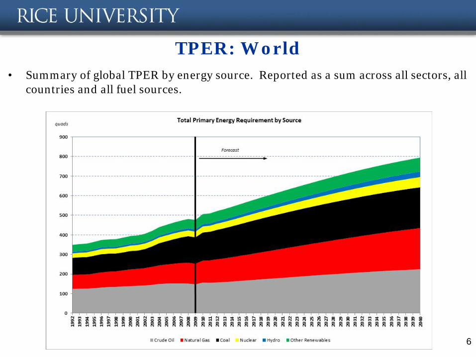
TPER: World • Summary of global TPER by energy source. Reported as a sum across all sectors, all

countries and all fuel sources.

6

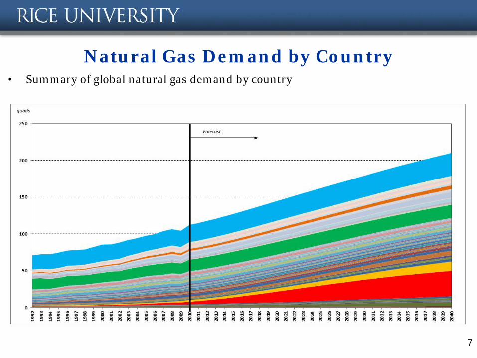
Natural Gas Demand by Country • Summary of global natural gas demand by country

7

Supply: Shale Resources and Costs

8

The RWGTM: Supply • Recall, there are over 135 regions

• Natural gas resources are represented as… – Conventional, CBM and Shale in North America, China, Europe and Australia,

and conventional gas deposits in the rest of the world. Changes incorporate the analysis of the recent ARI assessment of shale around the world.

• … in three categories – proved reserves (Oil & Gas Journal estimates)

– growth in known reserves (P-50 USGS and NPC 2003 estimates)

– undiscovered resource (P-50 USGS and NPC 2003 estimates) – Note: resource assessments are supplemented by regional offices if available.

• North American cost-of-supply estimates are econometrically related to play-level geological characteristics and applied globally to generate costs for all regions of the world.

– Long run costs increase with depletion.

– Short run adjustment costs limit the “rush to drill” phenomenon.

– We allow technological change to reduce mining costs longer term 9

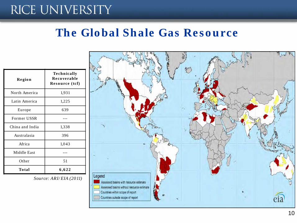
The Global Shale Gas Resource

Region

Technically Recoverable

Resource (tcf)

North America 1,931

Latin America 1,225

Europe 639

Former USSR ---

China and India 1,338

Australasia 396

Africa 1,043

Middle East ---

Other 51

Total 6,622

Source: ARI/EIA (2011)

10

11

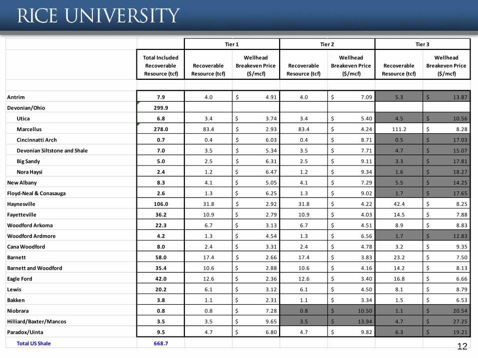
EURs in Shale Plays • EURs estimated using geologic data for known shale plays in North America and

econometrically fit for RoW shales. – EUR a function of porosity, TM, TOC, Clay Content, GIP Concentration, Thickness, Depth

– Tiers constructed with pdfs of EURs informed by average EUR and US well performance.

• Drilling and Completion costs estimated using known North American plays and econometrically fit to drilling depth and reservoir pressure.

12

Total Included Recoverable Resource (tcf)

Recoverable Resource (tcf)

Wellhead Breakeven Price

($/mcf)Recoverable

Resource (tcf)


($/mcf)Recoverable

Resource (tcf)


($/mcf)

Antrim 7.9 4.0 4.91$ 4.0 7.09$ 5.3 13.87$

Devonian/Ohio 299.9

Utica 6.8 3.4 3.74$ 3.4 5.40$ 4.5 10.56$

Marcellus 278.0 83.4 2.93$ 83.4 4.24$ 111.2 8.28$

Cincinnatti Arch 0.7 0.4 6.03$ 0.4 8.71$ 0.5 17.03$

Devonian Siltstone and Shale 7.0 3.5 5.34$ 3.5 7.71$ 4.7 15.07$

Big Sandy 5.0 2.5 6.31$ 2.5 9.11$ 3.3 17.81$

Nora Haysi 2.4 1.2 6.47$ 1.2 9.34$ 1.6 18.27$

New Albany 8.3 4.1 5.05$ 4.1 7.29$ 5.5 14.25$

Floyd-Neal & Conasauga 2.6 1.3 6.25$ 1.3 9.02$ 1.7 17.65$

Haynesville 106.0 31.8 2.92$ 31.8 4.22$ 42.4 8.25$

Fayetteville 36.2 10.9 2.79$ 10.9 4.03$ 14.5 7.88$

Woodford Arkoma 22.3 6.7 3.13$ 6.7 4.51$ 8.9 8.83$

Woodford Ardmore 4.2 1.3 4.54$ 1.3 6.56$ 1.7 12.83$

Cana Woodford 8.0 2.4 3.31$ 2.4 4.78$ 3.2 9.35$

Barnett 58.0 17.4 2.66$ 17.4 3.83$ 23.2 7.50$

Barnett and Woodford 35.4 10.6 2.88$ 10.6 4.16$ 14.2 8.13$

Eagle Ford 42.0 12.6 2.36$ 12.6 3.40$ 16.8 6.66$

Lewis 20.2 6.1 3.12$ 6.1 4.50$ 8.1 8.79$

Bakken 3.8 1.1 2.31$ 1.1 3.34$ 1.5 6.53$

Niobrara 0.8 0.8 7.28$ 0.8 10.50$ 1.1 20.54$

Hilliard/Baxter/Mancos 3.5 3.5 9.65$ 3.5 13.94$ 4.7 27.25$

Paradox/Uinta 9.5 4.7 6.80$ 4.7 9.82$ 6.3 19.21$

Total US Shale 668.7

Tier 3Tier 1 Tier 2

13




($/mcf)Recoverable

Resource (tcf)


($/mcf)Recoverable

Resource (tcf)


($/mcf)

Horn River/Cordova/Liard 158.5 56.7 3.69$ 48.6 5.33$ 53.2 10.42$

Montney/Deep Colorado 136.0 40.8 2.58$ 40.8 3.73$ 54.4 7.30$

Utica 27.0 8.1 2.89$ 8.1 4.17$ 10.8 8.16$

Horton Bluff 1.2 0.6 4.85$ 0.6 7.00$ 0.8 13.69$

Total Canadian Shale 321.5

Burgos/Sabinas (incl. Eagle Ford) 163.3 51.3 2.96$ 48.0 4.27$ 64.0 8.36$

Tampico/Tuxpan/Veracruz 33.3 18.0 3.64$ 15.3 5.26$ 20.4 10.29$

Total Mexican Shale 196.6

Maracaibo/Catatumbo (Venezuela) 7.5 5.4 4.62$ 2.1 6.67$ 2.8 13.04$

Catatumbo (Colombia) 7.2 3.6 2.98$ 3.6 4.30$ 4.8 8.41$

San Alfredo (Bolivia) 31.3 15.6 4.86$ 15.6 7.01$ 20.8 13.71$

San Alfredo (Brazil) 137.5 68.8 4.27$ 68.8 6.16$ 91.7 12.04$

San Alfredo (Paraguay) 40.6 20.3 4.54$ 20.3 6.56$ 27.1 12.82$

San Alfredo (Argentina) 103.2 51.6 4.27$ 51.6 6.16$ 68.8 12.04$

Neuquen (Argentina) 407.0 122.1 2.76$ 122.1 3.98$ 162.8 7.79$

San Jorge/Magallanes (Argentina) 160.2 80.1 4.38$ 80.1 6.32$ 106.8 12.35$

Total South American Shale 894.5

Australia (Cooper) 85.0 25.5 3.10$ 25.5 4.47$ 34.0 8.75$

Australia (Maryborough) 23.0 6.9 3.32$ 6.9 4.79$ 9.2 9.37$

Australia (Perth) 59.0 17.7 2.96$ 17.7 4.27$ 23.6 8.35$

Australia (Canning) 229.0 68.7 3.57$ 68.7 5.16$ 91.6 10.09$

Total Australian Shale 396.0

Tier 1 Tier 2 Tier 3

14




($/mcf)Recoverable

Resource (tcf)


($/mcf)Recoverable

Resource (tcf)


($/mcf)

Austria (Mikulov) 32.0 16.0 6.50$ 16.0 9.38$ 21.3 18.35$

Poland (Baltic) 77.4 38.7 6.68$ 38.7 9.64$ 51.6 18.86$

Poland (Lublin) 13.2 13.2 9.64$ 13.2 13.92$ 17.6 27.22$

Poland (Podlasie) 14.0 4.2 3.48$ 4.2 5.02$ 5.6 9.82$

Lithuania (Baltic) 13.8 6.9 6.68$ 6.9 9.64$ 9.2 18.86$

Ukraine (Dneiper-Donets) --- 3.6 18.21$ 3.6 26.29$ 4.8 51.41$

Ukraine (Lublin) 18.0 9.0 7.40$ 9.0 10.68$ 12.0 20.88$

France (Permian Carb) --- 22.8 17.68$ 22.8 25.52$ 30.4 49.91$

France (Terres Noires/Liassic) 62.4 31.2 4.58$ 31.2 6.60$ 41.6 12.92$

Germany (Posidonia/Wealden) 7.5 7.5 10.02$ 7.5 14.46$ 10.0 28.28$

Norway (Alum) 82.3 24.7 3.15$ 24.7 4.54$ 32.9 8.88$

Sweden (Alum) 41.2 12.3 3.22$ 12.3 4.65$ 16.5 9.09$

Denmark (Alum) 23.5 7.1 3.18$ 7.1 4.59$ 9.4 8.97$

UK (Bowland) 11.4 5.7 5.89$ 5.7 8.50$ 7.6 16.62$

UK (Liassic) 13.2 6.6 4.55$ 6.6 6.57$ 8.8 12.85$

Total European Shale 409.9

Algeria (Ghadames) 63.1 63.1 8.87$ 63.1 12.80$ 84.1 25.04$

Algeria (Tindouf) --- 15.0 15.31$ 15.0 22.10$ 20.0 43.23$

Tunisia (Ghadames) 6.2 6.2 8.51$ 6.2 12.29$ 8.3 24.03$

Libya (Sirt/Etel) 81.9 81.9 7.83$ 81.9 11.30$ 109.2 22.10$

Morocco (Tadla) --- 0.9 14.65$ 0.9 21.15$ 1.2 41.37$

South Africa (Prince Albert/Whitehill/Collingham) 145.5 145.5 10.34$ 145.5 14.93$ 194.0 29.19$

Total African Shale 296.7

China (Sichuan-Longmaxi/Qiongzhusi) 415.2 207.6 7.15$ 207.6 10.33$ 276.8 20.20$

China (Tarim-O1,O2,O3 Shales/Cambrian) 349.8 174.9 6.87$ 174.9 9.92$ 233.2 19.40$

India (Cambay/Indus) 24.0 12.0 6.25$ 12.0 9.03$ 16.0 17.65$

India (Damodar/Krishna) 20.4 10.2 4.11$ 10.2 5.93$ 13.6 11.60$

India (Cauvery) 5.4 2.7 5.47$ 2.7 7.90$ 3.6 15.45$

Pakistan (Indus) 18.6 9.3 4.19$ 9.3 6.05$ 12.4 11.83$

Turkey (Anatolia) 5.4 2.7 6.73$ 2.7 9.71$ 3.6 18.99$

Turkey (Thrace) 1.8 1.8 10.31$ 1.8 14.89$ 2.4 29.11$

Total Asian Shale 840.6

Tier 1 Tier 2 Tier 3

15

Region Country Country Total Region Total

US 668.7

Canada 321.5

Mexico 196.6

Argentina 670.4

Bolivia 31.3

Brazil 137.5

Colombia 7.2

Paraguay 40.6

Venezuela 7.5

Austria 32.0

Denmark 23.5

France 62.4

Germany 7.5

Lithuania 13.8

Norway 82.3

Poland 104.6

Sweden 41.2

Ukraine 18.0

UK 24.6

Algeria 63.1

Tunisia 6.2

Libya 81.9

South Africa 145.5

Australia 396.0

China 765.0

India 49.8

Pakistan 18.6

Turkey 7.2

4024.5

Africa

World

Asia & Oceania


1186.8

894.5

409.9

296.7

1236.6

South America

North America

Europe

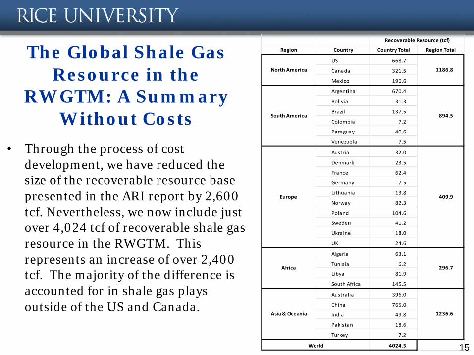
The Global Shale Gas Resource in the

RWGTM: A Summary Without Costs

• Through the process of cost development, we have reduced the size of the recoverable resource base presented in the ARI report by 2,600 tcf. Nevertheless, we now include just over 4,024 tcf of recoverable shale gas resource in the RWGTM. This represents an increase of over 2,400 tcf. The majority of the difference is accounted for in shale gas plays outside of the US and Canada.

LNG Shipping

16

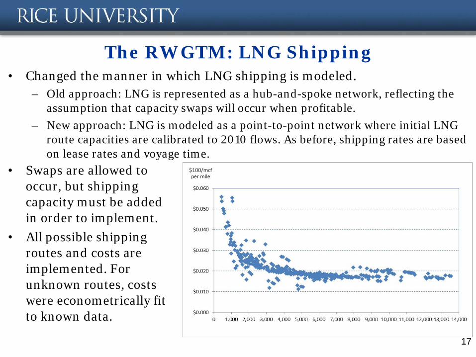
The RWGTM: LNG Shipping • Changed the manner in which LNG shipping is modeled.

– Old approach: LNG is represented as a hub-and-spoke network, reflecting the assumption that capacity swaps will occur when profitable.

– New approach: LNG is modeled as a point-to-point network where initial LNG route capacities are calibrated to 2010 flows. As before, shipping rates are based on lease rates and voyage time.

17

• Swaps are allowed to occur, but shipping capacity must be added in order to implement.

• All possible shipping routes and costs are implemented. For unknown routes, costs were econometrically fit to known data.

Reference Case Results

18

Reference Case: Demand by Super-Region, 2011-2040

• Asian demands, China and India in particular, set the trend for global natural gas demand growth.

19

Reference Case: Supply by Super-Region, 2011-2040

• Highest growth rates are seen in Asia where demands grow rapidly, shale gas resources are large, and existing production is relatively low.

20

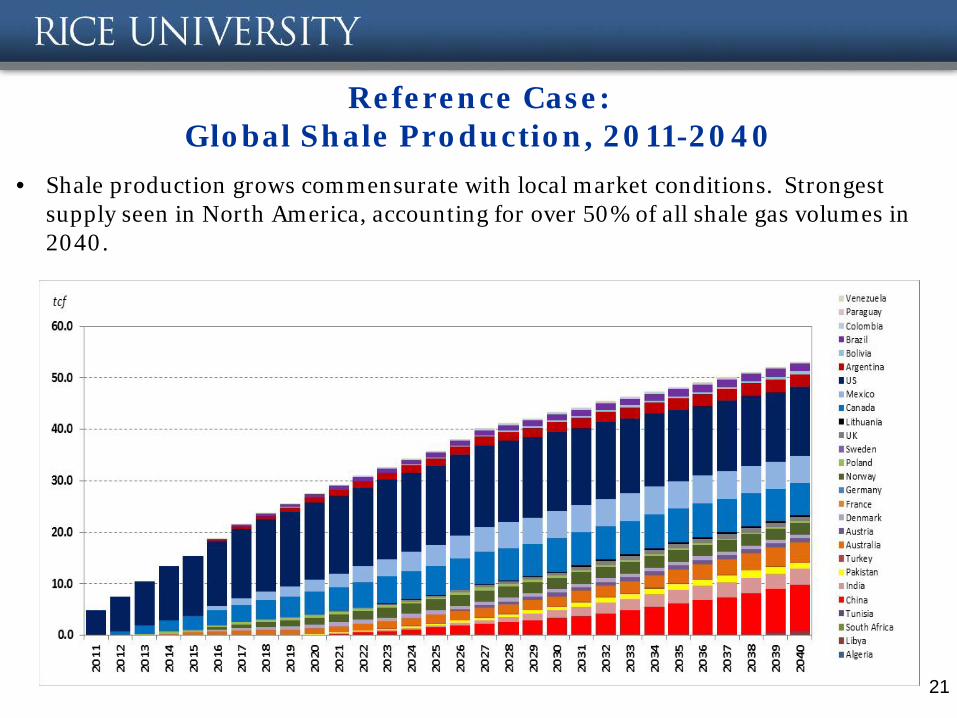
Reference Case: Global Shale Production, 2011-2040

21

• Shale production grows commensurate with local market conditions. Strongest supply seen in North America, accounting for over 50% of all shale gas volumes in 2040.

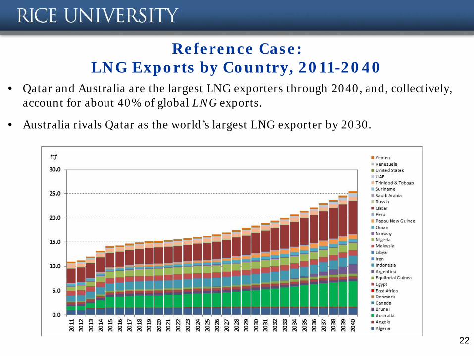
Reference Case: LNG Exports by Country, 2011-2040

• Qatar and Australia are the largest LNG exporters through 2040, and, collectively, account for about 40% of global LNG exports.

• Australia rivals Qatar as the world’s largest LNG exporter by 2030.

22

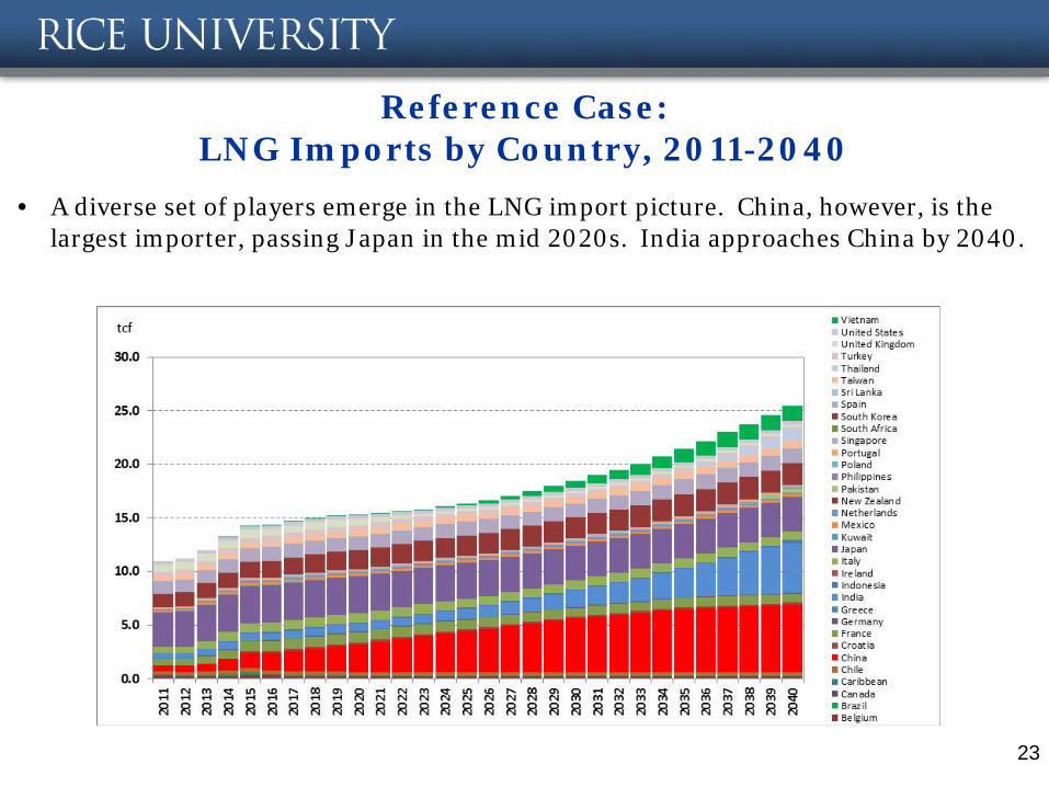
Reference Case: LNG Imports by Country, 2011-2040

• A diverse set of players emerge in the LNG import picture. China, however, is the largest importer, passing Japan in the mid 2020s. India approaches China by 2040.

23

Reference Case: Global Marker Prices, 2011-2040

• Note, the US price is Henry Hub, the European price is NBP, and the Asian price is the Japanese price paid for spot LNG. Global prices remain above the US price. The prices indicated are spot prices not contract prices.

24

Key Drivers

• Iran, Venezuela, Saudi Arabia, Qatar, etc. Energy supply decisions motivated by political considerations both directly and indirectly.

• Policy-driven energy choices, such as long term commitment to renewables.

• Political and regulatory circumstances that do not support investment – Nationalization (Argentina and YPF).

– Regime change

• Substantial changes in costs and/or access to resources

25

Key Drivers • The existence of regionally discrete natural gas markets around the globe

has persisted due to a lack of capability to directly arbitrage price differences. This is due to several factors, including, but not limited to,

- the existence of transportation monopolies,

- high costs of entry and long lead times for LNG and long haul pipeline capacity,

- lack of storage capacity and basic hub services in Asian and European markets,

- regulatory frameworks that do not encourage entry and entrepreneurial activity, particularly in the upstream sector (for example regarding property rights for minerals),

- regulatory frameworks that support the existence of monopolies in transportation and distribution (for example a lack of market oversight that forces unbundling), and

- lack of physical and financial market liquidity which masks price discovery, which in turn would signal infrastructure opportunities. This is a direct result of the other factors.

Anything altering these points will have a profound impact on the global gas market. 26

Appendix

27

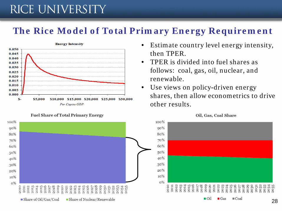
The Rice Model of Total Primary Energy Requirement

28

• Estimate country level energy intensity, then TPER.

• TPER is divided into fuel shares as follows: coal, gas, oil, nuclear, and renewable.

• Use views on policy-driven energy shares, then allow econometrics to drive other results.

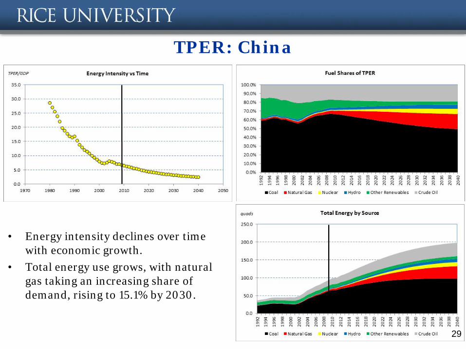
TPER: China

• Energy intensity declines over time with economic growth.

• Total energy use grows, with natural gas taking an increasing share of demand, rising to 15.1% by 2030.

29

TPER: India


• Total energy use grows, with natural gas taking an increasing share of demand, rising to 13.5% by 2030.

30

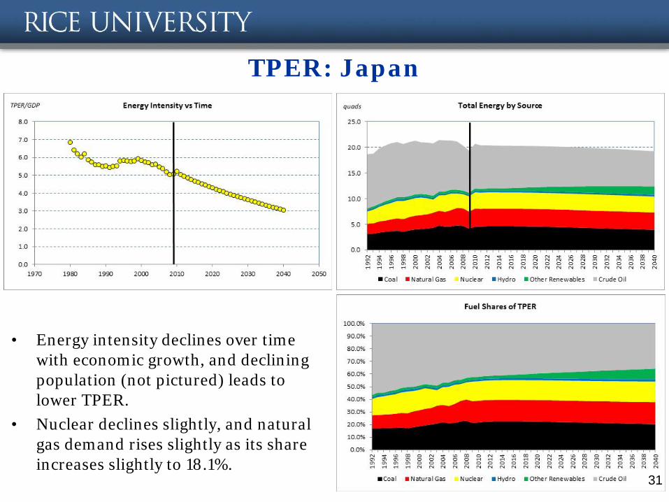
TPER: Japan

• Energy intensity declines over time with economic growth, and declining population (not pictured) leads to lower TPER.

• Nuclear declines slightly, and natural gas demand rises slightly as its share increases slightly to 18.1%.

31

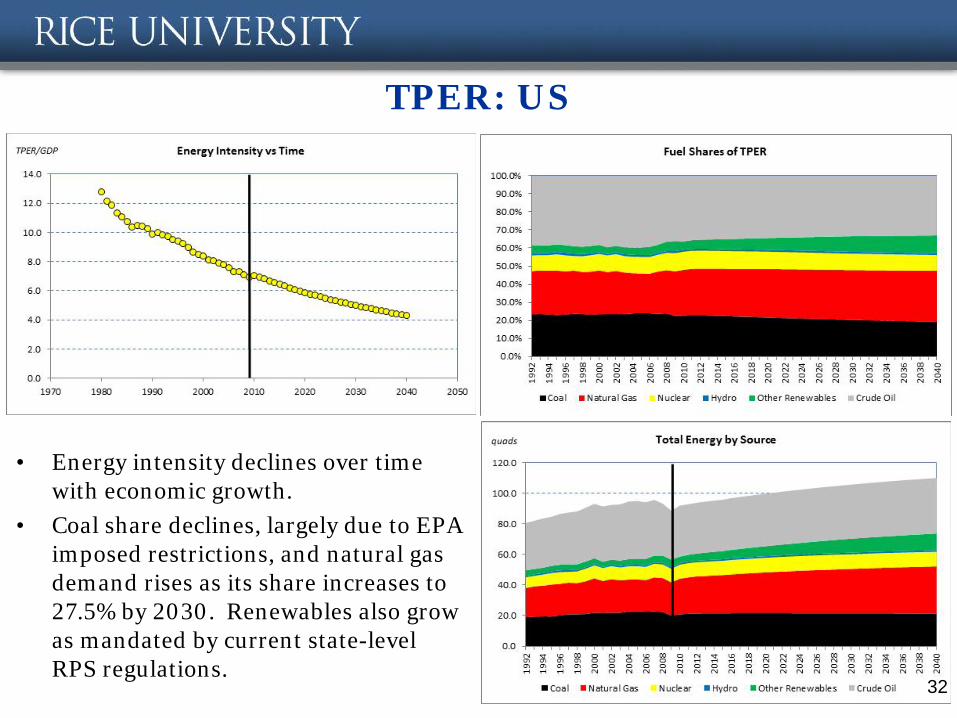
TPER: US


• Coal share declines, largely due to EPA imposed restrictions, and natural gas demand rises as its share increases to 27.5% by 2030. Renewables also grow as mandated by current state-level RPS regulations.

32

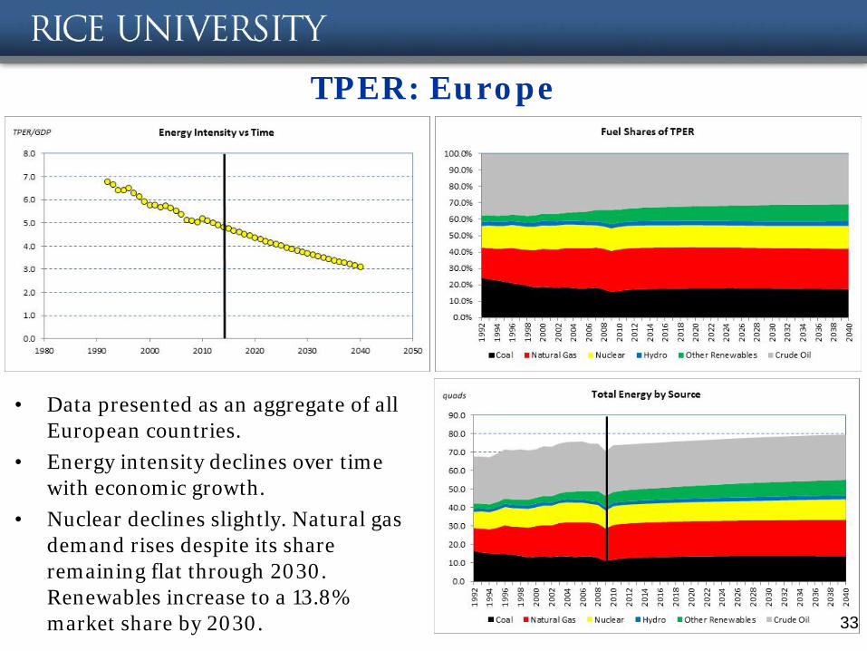
TPER: Europe

• Data presented as an aggregate of all European countries.


• Nuclear declines slightly. Natural gas demand rises despite its share remaining flat through 2030. Renewables increase to a 13.8% market share by 2030. 33

Documents

The Rice World Gas Trade Model (RWGTM)