0

The Rising Postgraduate Wage Premium

Joanne Lindley*and Stephen Machin **

October 2013

* Department of Management, King’s College London

** Department of Economics, University College London and Centre for EconomicPerformance, London School of Economics

Abstract

This paper documents significant increases in the number of postgraduates in the labourmarket and reports that their relative wages have significantly risen over time in the UnitedStates and in Great Britain, both compared to all other workers and compared to othergraduates with only a college degree. Part of the reason why is that postgraduates and collegeonly workers have different skill sets, do different jobs and are therefore imperfect substitutesin production. Because of this, relative demand has shifted faster over time in favour ofpostgraduates. The skills and job tasks performed by postgraduates complement computersmore and thus they have benefited more from their spread than have college only workers. Asa consequence, the growing presence of postgraduates has been an important factor inexplaining rising wage inequality amongst college graduates and in accounting for labourmarket polarization at the top of the skill distribution.

JEL Keywords: Relative wages; Postgraduate education; Computers; Polarization.

JEL Classifications: J24; J31

Author Emails: joanne.lindley@kcl.ac.uk; s.machin@ucl.ac.uk

Acknowledgements

This is a revised version of a previous paper entitled “Rising Wage Inequality andPostgraduate Education” (Lindley and Machin, 2011). We would like to thank participants in anumber of seminars and conferences for helpful comments and suggestions.

1

1. Introduction

Rising wage differentials between education groups have been identified as a key feature of

rising wage inequality in a number of countries (most notably the US and UK, but also

elsewhere).1 Rising relative wages for college educated workers, despite their increased

numbers, and the increased relative demand for workers that are more educated (and the

drivers of these increases) have featured prominently in discussions of why overall wage

inequality has risen.

One feature of the increased supply of college educated workers is that over time more

individuals have not stopped their education once graduating with a first degree. Rather, they

have gone on to acquire postgraduate qualifications. In fact, in 2010 in both the countries we

study in this paper (the United States and Great Britain) over 10 percent of the adult workforce

(or 36 percent of all college graduates) have a postgraduate qualification.

Study of the increased importance of postgraduate education in the labour market has

to date not received much direct attention from the contributors to the rising wage inequality

literature. Postgraduate education does feature as a focus of one US paper (by Eckstein and

Nagypal, 2004) which studies trends in overall wage inequality in the US from 1961 to 2002

and, unlike others in the literature, does highlight rising wage differentials for workers with

postgraduate degrees. Also, whilst not their main focus, several references are made to rising

post-college wages in Autor, Katz and Kearney’s (2008) study of rising wage gaps between

more and less educated workers in the US.2

In terms of the potential importance of the issue, it is noteworthy that when Lemieux

(2006a) looks at all postsecondary education, rather than just college only graduates, in a

decomposition of inequality changes between the mid-1970s and mid-2000s he concludes that

‘Understanding why postsecondary education, opposed to other observed or unobserved

1 See Acemoglu and Autor (2010) for an up to date review of this literature.2 Acemoglu and Autor (2010) also present charts showing faster wage growth amongst the postgraduate groupand the 'convexification' of the wage returns to education over time that has resulted from this.

2

measures of skills, plays such a dominant role in changes in wage inequality should be an

important priority for future research' [Lemieux, 2006a, p.199].

Much of the existing wage differentials literature (at least as its starting point) bases

itself on what has become known as the canonical model of relative supply and demand (see,

among others, Tinbergen, 1974; Katz and Murphy, 1992; Acemoglu and Autor, 2010;

Carneiro and Lee, 2011). In this model, wage differentials between workers with different

education levels are empirically related to measures of the relative supply of the different

groups and proxies for demand (usually trends assumed to be driven by technical change). The

focus is usually placed on studying particular wage differentials (usually the college only/high

school or college plus/high school wage gap) and modelling labour supply for just two

(aggregated) education groups: ‘college equivalent’ workers and ‘high school equivalent’

workers (see, inter alia, the influential US papers of Katz and Murphy, 1992, Card and

Lemieux, 2001, and Autor, Katz and Kearney, 2008).3 More recent work (like Carneiro and

Lee, 2011) considers the question as to why the college/high school wage premium has not

continued to increase as fast as before, but does not separately look at post-college workers.

In the canonical approach as typically implemented, postgraduates and college only

workers are distinguished via constant efficiency weights (based on their relative wages) in the

college equivalent labour supply group. This (implicitly) presumes postgraduates to be more

productive versions of college only workers, but also that they do the same jobs and so end up

being perfect substitutes in production. In this paper, we present several pieces of evidence to

the contrary. First, estimates of the canonical model reveal evidence of imperfect

3 In their estimation of relative supply-demand models in the US labour market, these authors make assumptionson the labour supply of the following five groups of workers: workers with a high school degree supply one‘high school equivalent’, whilst workers with less than a high school degree supply a (constant relative wageweighted) proportion of this; workers with a college degree supply one ‘college equivalent’, whilst workers witha postgraduate degree supply a (constant relative wage weighted) mark up of this; and, finally, the intermediategroup with some college are split between the two groups (Katz and Murphy, 1992, and Autor, Katz andKearney, 2008, split them 50-50, whilst Card and Lemieux, 2001, assume they supply α high school equivalents and (1-α) college equivalents, where α is a high school weight used to measure the wages of some college workers as a weighted mean of high school and college wages.

3

substitutability between postgraduate and college only workers. Second, the skills and job

tasks done by postgraduates and college only workers are shown to be different, as are in the

occupations in which the two groups of graduates work.

The canonical model estimates we present also show that, whilst relative demand shifts

have favoured all college graduates relative to other workers so that relative wages of all

graduates have risen, it turns out that demand has shifted faster for postgraduates so that

within the college graduate group this has significantly widened the wage gap between

postgraduates and college only workers. Further examination of the relative demand shifts

reveals that postgraduates more highly complement computers and thus have benefited more

from their spread than have college only workers, in part because of the skills sets they

possess. Hence, overall, the growing presence of postgraduates in the workplace has been an

important factor behind rising wage inequality amongst graduates. So too has their increased

employment in higher skill jobs been an important aspect of the polarization of the labour

market that has been seen in recent decades.4

The rest of the paper is structured as follows. In Section 2, we present initial

descriptive evidence on changes in the relative wages of postgraduates and college only

workers. In Section 3, we show results from estimating models of the relative demand and

supply of workers with different levels of education, placing a specific focus on estimating

differential supply and demand effects for postgraduate versus college only workers. We also

look at differences in the skills and job tasks of postgraduate and college only workers, and the

occupations of these groups of workers. Section 4 explores the nature of relative demand shifts

in more detail by looking at differences in technology complementarities for postgraduates as

4 See the review of Acemoglu and Autor (2010), and the series of US papers by Autor and colleagues (beginningwith Autor, Levy and Murnane, 2003, and also Autor, Katz and Kearney, 2008, and Autor and Dorn, 2013).European papers showing job polarization in Europe include Goos and Manning (2007) for the UK, Spitz-Oener(2006) for Germany and Goos, Manning and Salomons (2009) for a number of countries. Michaels, Natraj andVan Reenen (2013) present evidence that polarization connected to computerization is pervasive across a numberof countries.

4

compared to college only workers, and by looking at how the growth of postgraduate

employment in high skill jobs is a feature of labour market polarization. Finally, Section 5

concludes.

2. Changes in Postgraduate Employment and Wages

Rising Wage Inequality and Education

The broad motivation underpinning this paper comes from changing wage and employment

structures with rapid labour market inequality increases in the United States and Great Britain

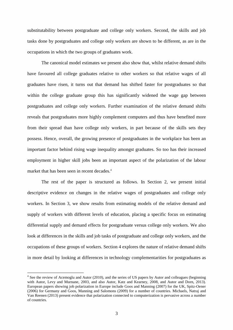
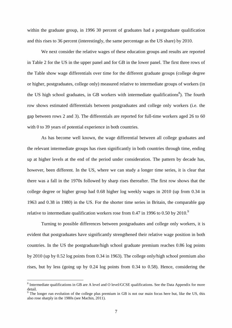
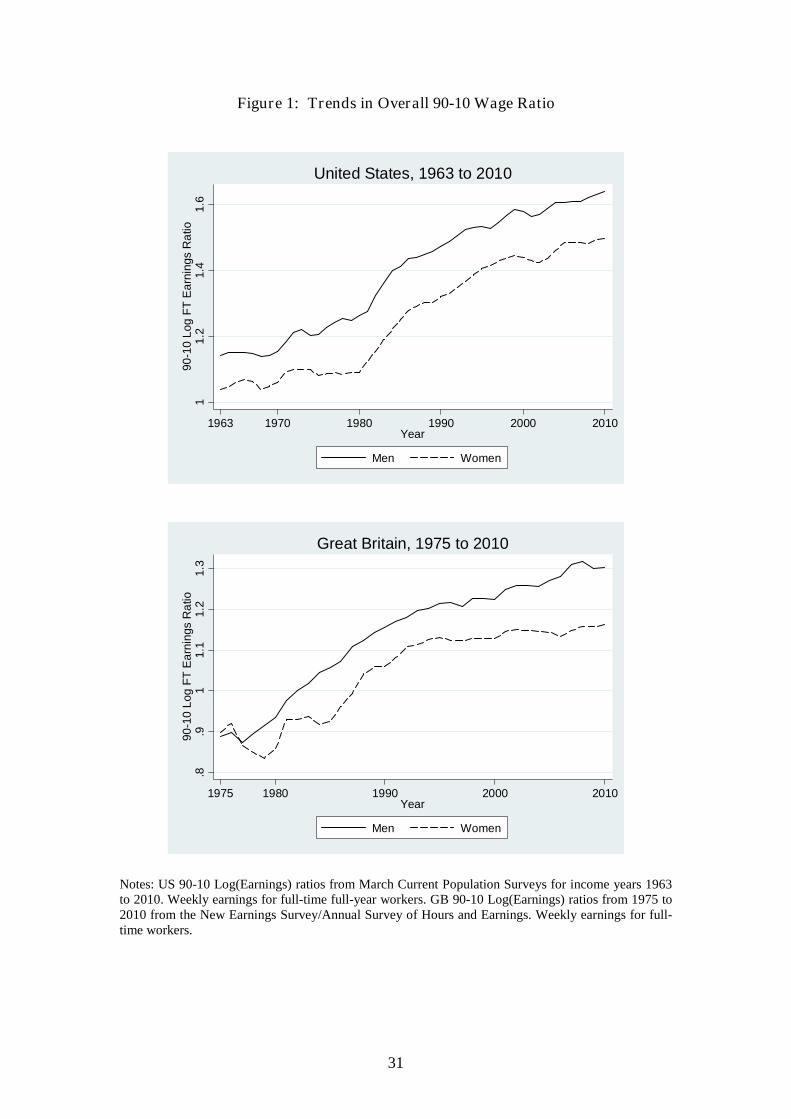
over the last thirty to forty years. To see this, Figure 1 shows the 90-10 ratio of log (weekly

wages) for full-time workers (and for the US, full-year workers) from the March Current

Population Survey (CPS) for the United States and New Earnings Survey/Annual Survey of

Hours and Earnings (NES/ASHE) for Great Britain.5 The Figure shows the evolution of the

90-10 ratio for men and women in the US between 1963 and 2010 and for GB between 1975

and 2010. In both countries, for both sexes, overall wage inequality measured by the 90-10

stands at a substantially higher level in the final year, and there is a strong trend upwards in

both countries starting from somewhere around the late 1960s in the US and the late 1970s in

Britain.

As noted in the introduction, a focus in the literature on understanding rising wage

inequality has been to study between-group and within-group changes in inequality. By far the

most attention in the former category has been on studying wage gaps between workers with

different education levels, as rising wage gaps between high and low education workers have

been shown to be important determinants of rises in overall wage inequality (see the reviews

of Katz and Autor, 1999, and Acemoglu and Autor, 2010, for more details).

5 The March CPS is used for the US as it has a time series with wage and education data running as far back as1963. The NES/ASHE data is used for GB as it has wage data back to 1970. However, it does not contain aneducation variable and so we cannot go as far back in our analysis that requires education data for GB - for thiswe use a combination of General Household Survey data (from 1977 to 1992) and the much larger sample sizesfrom the Labour Force Survey (from 1993 onwards when it first recorded earnings information).

5

In the existing work, however, the emphasis has to date mostly been placed on

studying the evolution through time of rather narrowly defined wage differentials. For

example, the influential US papers of Katz and Murphy (1992), Card and Lemieux (2001) and

Autor, Katz and Kearney (2008) all consider the evolution through time of one specific

educational wage differential, the college only/high school graduate wage gap (i.e. the wage

gap between workers with exactly 16 and 12 years of education).

The fixed four year gap in schooling between college only and high school graduates

has the advantage of being consistently defined measure of the college wage premium.

However, it does select a specific group of graduates, eliminating those with more advanced

postgraduate qualifications. Contributors to this literature are certainly aware of this and

sometimes report additional estimates looking at the wage gap between workers with 16 or

more years of education (i.e. college only and postgraduates, or college plus) as compared to

workers with a high school degree. In Card and Lemieux’s (2001) analysis, for example, they

state that, based on data running up to 1995, it makes little difference. However, as we have

already noted, aggregating college only and postgraduates workers into one composite group

presumes them to be perfect substitutes and therefore that their relative wages (net of supply)

should have remained constant over time.

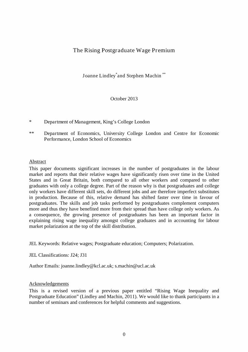
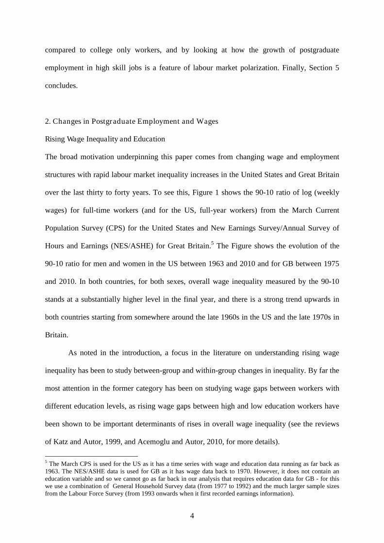
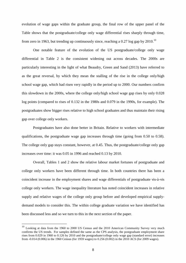
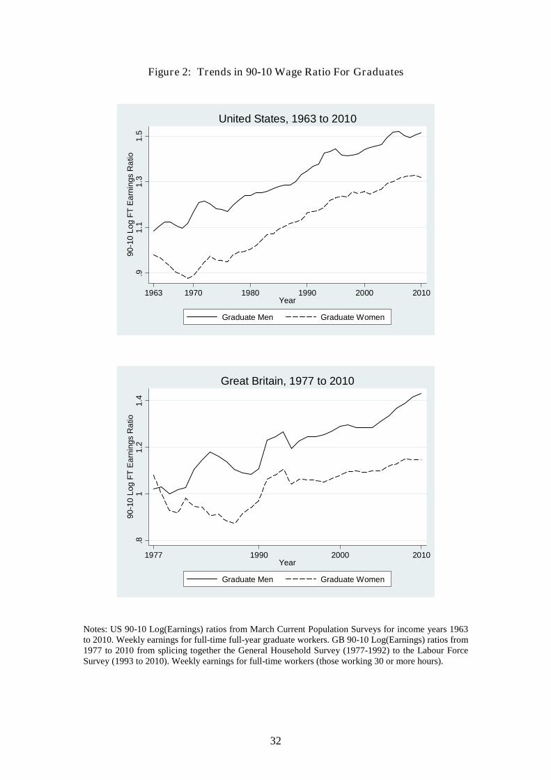
We believe there are good reasons to revisit this. First, wage inequality has risen

within the college plus group. Figure 2 shows the 90-10 ratio for all male and female

graduates in the US and GB samples, again running from 1963 to 2010 in the US and now

(because of requiring a consistent education variable) from 1977 to 2010 in GB using the

General Household Survey (1977 to 1992) and Labour Force Survey (1993 to 2010). The

Figure shows significant rises in graduate wage inequality. Second, the relative employment

and wages of postgraduate versus college only workers have shifted substantially through

6

time. This is especially the case in time periods after the data used in existing work that does

consider both college only and college plus measures. We show this in the next sub-section.

Trends in Postgraduate Employment and Wages

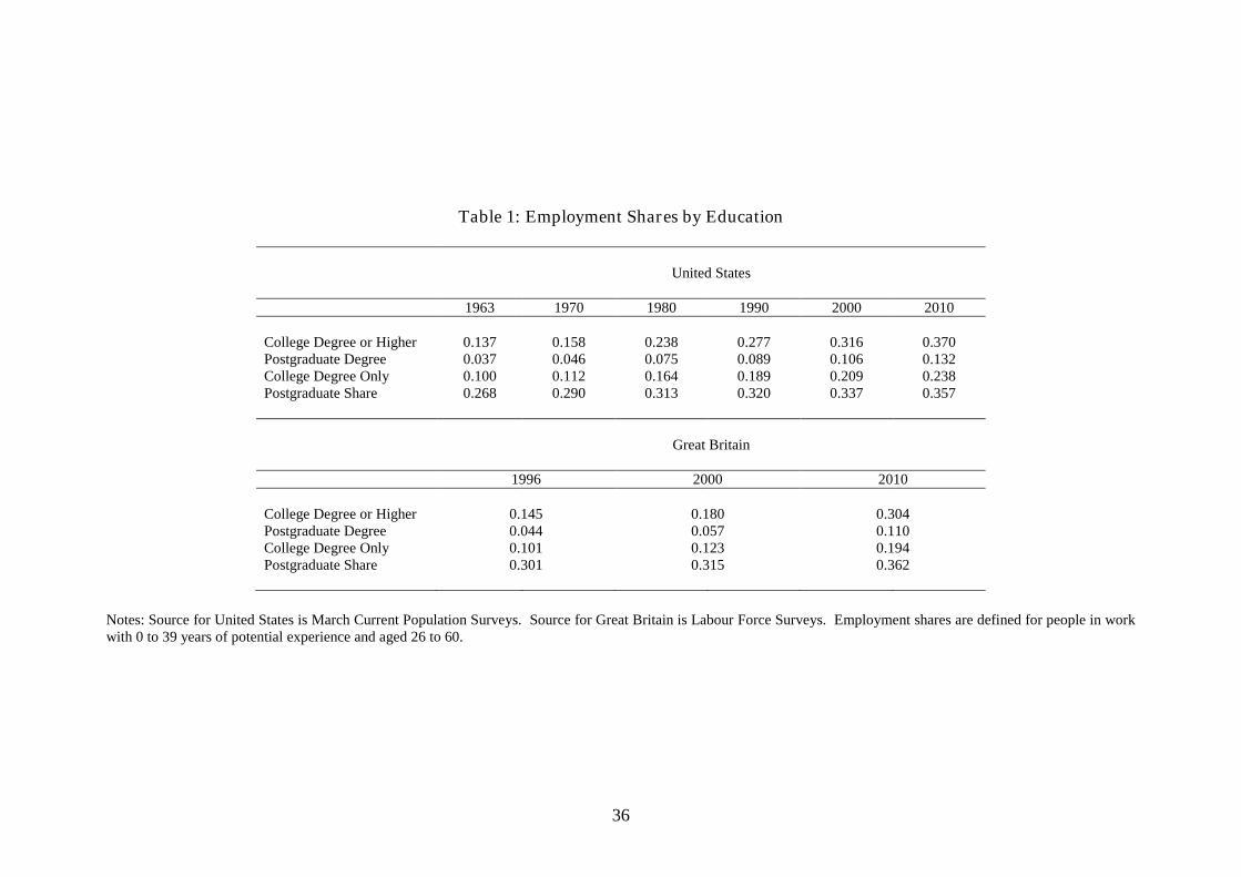
Table 1 shows the employment shares of all graduates (college degree or higher),

postgraduates and college only employment shares and the postgraduate share amongst

graduates for the United States and Great Britain over time. The upper panel of the Table

shows that the overall graduate proportion is higher in the US, and has risen from 0.14 in 1963

through to 0.37 by 2010.6 The decade by decade changes reveal a well known pattern, where

the employment share of graduates rose rapidly in the 1970s, and continued to rise at a slower

rate in the decades that followed. Considering the postgraduate and college only proportions,

they broadly show the same decade by decade pattern of change, although the overall change

is faster for postgraduates whose graduate share rises to 36 percent of graduates by 2010 (up

from 27 percent in 1963).

The GB numbers are in the lower panel of the Table. These are taken from the Labour

Force Survey (LFS) and are reported from 1996 to 2010, since the definition of postgraduate

qualifications is only consistent from 1996 onwards. There is a rapid increase in the share of

all graduates in employment (from 0.15 in 1996 to 0.30 by 2010). This reflects a longer run

rapid increase in the graduate share, which has which speeded up through time.7

In the 1996 to 2010 period, there is also a sharper increase in the postgraduate share,

from 0.044 in 1996, rising to 0.110 of the workforce in 2010. In terms of changing shares

6 In the early 1990s, the education variable changed definition in the US and after the definition change one canidentify whether postgraduates hold a master's degree, a professional qualification or a doctoral degree. Lookingat trends in these shows that a large part of the increased number of people holding a postgraduate degree wasdue to a rise in masters degrees (which are typically two year post-bachelor degrees). Sample sizes and theshorter time series on this breakdown precluded us undertaking any detailed analysis of these patterns of changealthough Tables showing descriptive statistics are available from the authors on request.7 See Machin (2011) and Walker and Zhu (2008). The graduate share was around 6 percent in 1977 and thereforegraduate supply has increased very rapidly through time, in part reflecting the expansion of higher education thatoccurred in the early 1990s (see Devereux and Fan, 2011, or Machin and Vignoles, 2005).

7

within the graduate group, in 1996 30 percent of graduates had a postgraduate qualification

and this rises to 36 percent (interestingly, the same percentage as the US share) by 2010.

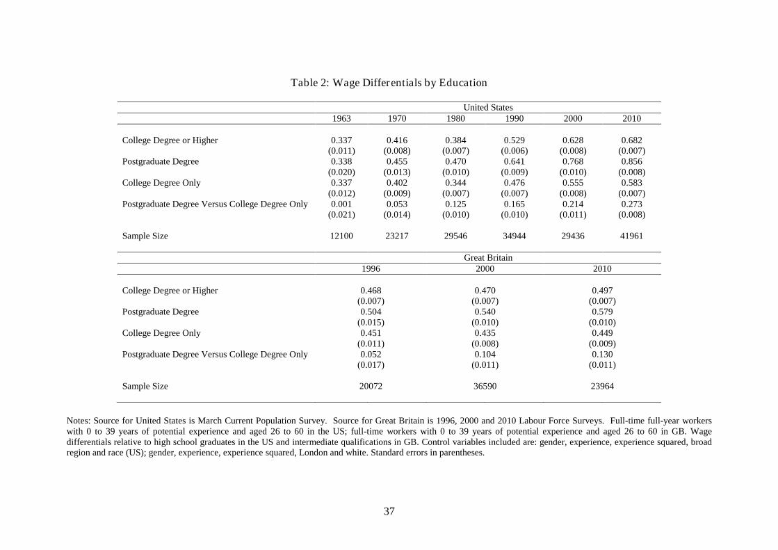
We next consider the relative wages of these education groups and results are reported

in Table 2 for the US in the upper panel and for GB in the lower panel. The first three rows of

the Table show wage differentials over time for the different graduate groups (college degree

or higher, postgraduates, college only) measured relative to intermediate groups of workers (in

the US high school graduates, in GB workers with intermediate qualifications8). The fourth

row shows estimated differentials between postgraduates and college only workers (i.e. the

gap between rows 2 and 3). The differentials are reported for full-time workers aged 26 to 60

with 0 to 39 years of potential experience in both countries.

As has become well known, the wage differential between all college graduates and

the relevant intermediate groups has risen significantly in both countries through time, ending

up at higher levels at the end of the period under consideration. The pattern by decade has,

however, been different. In the US, where we can study a longer time series, it is clear that

there was a fall in the 1970s followed by sharp rises thereafter. The first row shows that the

college degree or higher group had 0.68 higher log weekly wages in 2010 (up from 0.34 in

1963 and 0.38 in 1980) in the US. For the shorter time series in Britain, the comparable gap

relative to intermediate qualification workers rose from 0.47 in 1996 to 0.50 by 2010.9

Turning to possible differences between postgraduates and college only workers, it is

evident that postgraduates have significantly strengthened their relative wage position in both

countries. In the US the postgraduate/high school graduate premium reaches 0.86 log points

by 2010 (up by 0.52 log points from 0.34 in 1963). The college only/high school premium also

rises, but by less (going up by 0.24 log points from 0.34 to 0.58). Hence, considering the

8 Intermediate qualifications in GB are A level and O level/GCSE qualifications. See the Data Appendix for moredetail.9 The longer run evolution of the college plus premium in GB is not our main focus here but, like the US, thisalso rose sharply in the 1980s (see Machin, 2011).

8

evolution of wage gaps within the graduate group, the final row of the upper panel of the

Table shows that the postgraduate/college only wage differential rises sharply through time,

from zero in 1963, but trending up continuously since, reaching a 0.27 log gap by 2010.10

One notable feature of the evolution of the US postgraduate/college only wage

differential in Table 2 is the consistent widening out across decades. The 2000s are

particularly interesting in the light of what Beaudry, Green and Sand (2013) have referred to

as the great reversal, by which they mean the stalling of the rise in the college only/high

school wage gap, which had risen very rapidly in the period up to 2000. Our numbers confirm

this slowdown in the 2000s, where the college only/high school wage gap rises by only 0.028

log points (compared to rises of 0.132 in the 1980s and 0.079 in the 1990s, for example). The

postgraduates show bigger rises relative to high school graduates and thus maintain their rising

gap over college only workers.

Postgraduates have also done better in Britain. Relative to workers with intermediate

qualifications, the postgraduate wage gap increases through time (going from 0.50 to 0.58).

The college only gap stays constant, however, at 0.45. Thus, the postgraduate/college only gap

increases over time: it was 0.05 in 1996 and reached 0.13 by 2010.

Overall, Tables 1 and 2 show the relative labour market fortunes of postgraduate and

college only workers have been different through time. In both countries there has been a

coincident increase in the employment shares and wage differentials of postgraduate vis-à-vis

college only workers. The wage inequality literature has noted coincident increases in relative

supply and relative wages of the college only group before and developed empirical supply-

demand models to consider this. The within college graduate variation we have identified has

been discussed less and so we turn to this in the next section of the paper.

10Looking at data from the 1960 to 2000 US Census and the 2010 American Community Survey very much

confirms the US trends. For samples defined the same as the CPS analysis, the postgraduate employment sharerises from 0.029 in 1960 to 0.126 by 2010 and the postgraduate/college only wage gap (standard error) increasesfrom -0.014 (0.006) in the 1960 Census (for 1959 wages) to 0.256 (0.002) in the 2010 ACS (for 2009 wages).

9

3. Relative Supply-Demand Models

In this section we consider how the relative wage and employment patterns documented in the

previous section of the paper map into shifts in the relative demand and supply of graduate

workers with postgraduate and college only education. Our strategy is to draw upon

established methods from the existing literature, so we begin by presenting estimates of what

has become known as the canonical model of relative supply and demand, where relative wage

differentials by education are empirically related to measures of the relative supply and

proxies for demand (usually trends assumed to be driven by technical change). This approach

was formalised in a general way by Katz and Murphy (1992) and has been empirically

estimated by a number of authors since (see Acemoglu and Autor, 2010).

The starting point in this approach is a Constant Elasticity of Substitution production

function where output in period t (Yt) is produced by two education groups (E1t and E2t) with

associated technical efficiency parameters (θ1t and θ2t) as follows:

1/ρρ2t2t

ρ1t1tt )EθE(θY (1)

where ρ = 1 – 1/σE, where σE is the elasticity of substitution between E1t and E2t.

Equating wages to marginal products for each education group, taking logs and

expressing as a ratio leads to the relative wage equation

2t

1t

E2

1

2t

1t

E

Elog

1-log

W

Wlog

t

t that can

be transformed by parameterising the demand shifts term as t102t

1t e t αα θ

θlog

, where t is a

time trend and et is an error term, to give

t2t

1t210

2t

1t eE

Elogt

W

Wlog

(2)

where α2 = –1/σE.

Thus, the relative wage is a function of a linear trend and relative supply. The typical

approach for estimating (2) focuses on a narrowly defined wage differential (usually the

10

college only/high school gap) and models supply in terms of college equivalent and high

school equivalent workers. To define equivalents within the college and high school groups,

individuals with different education are assumed to be perfect substitutes, but are given

different efficiency weights. So, for example, in terms of defining college equivalents,

postgraduates are assumed to be perfect substitutes for college only graduates but they are

given a higher relative efficiency (e.g. in some work of around 125% which is assumed

constant over time).

This assumption of perfect substitutability, but different efficiency weightings,

effectively says postgraduates do the same jobs as college only workers, but are just more

productive. It presumes therefore that their relative wages should have been constant through

time, a presumption that is at odds with the descriptive wage trends we showed in the previous

section of the paper (and as also remarked upon noted by Autor, Katz and Kearney, 2008).

Card and Lemieux (2001) have noted that the above model also imposes the restriction

that different age or experience groups with the same education level are perfect substitutes,

an assumption that is not consistent with the US data they analyse where the wage differentials

between college only and high school graduates do not move in the same way for different age

or experience groups through time.11 One can relax this assumption by decomposing E1t and

E2t into CES sub-aggregates as

1/η

j

η1jt1j1t EβE

and

1/η

j

η2jt2j2t EβE

, where there are j

age or experience groups and η = 1 – 1/σX, where σX is the elasticity of substitution between

different experience or age groups within the same education level.12

11 They show that the college only/high school graduate wage rises faster over time for younger and workers withlower potential experience.12 Of course, if η = 1 (because σX is infinity owing to perfect substitution) this collapses back to the standardKatz-Murphy model. Notice we use X denoting experience as notation here as we focus on substitution acrossexperience groups for most of our analysis (much the same emerged if we looked at substitution across agegroups as well - these results are available on request from the authors).

11

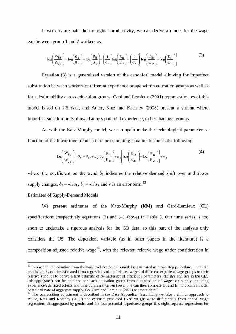
If workers are paid their marginal productivity, we can derive a model for the wage

gap between group 1 and 2 workers as:

2t

1t

2jt

1jt

X2t

1t

E2j

1j

2t

1t

2jt

1jt

E

Elog

E

Elog

σ

1

E

Elog

σ

1

β

βlog

θ

θlog

W

Wlog

(3)

Equation (3) is a generalised version of the canonical model allowing for imperfect

substitution between workers of different experience or age within education groups as well as

for substitutability across education groups. Card and Lemieux (2001) report estimates of this

model based on US data, and Autor, Katz and Kearney (2008) present a variant where

imperfect substitution is allowed across potential experience, rather than age, groups.

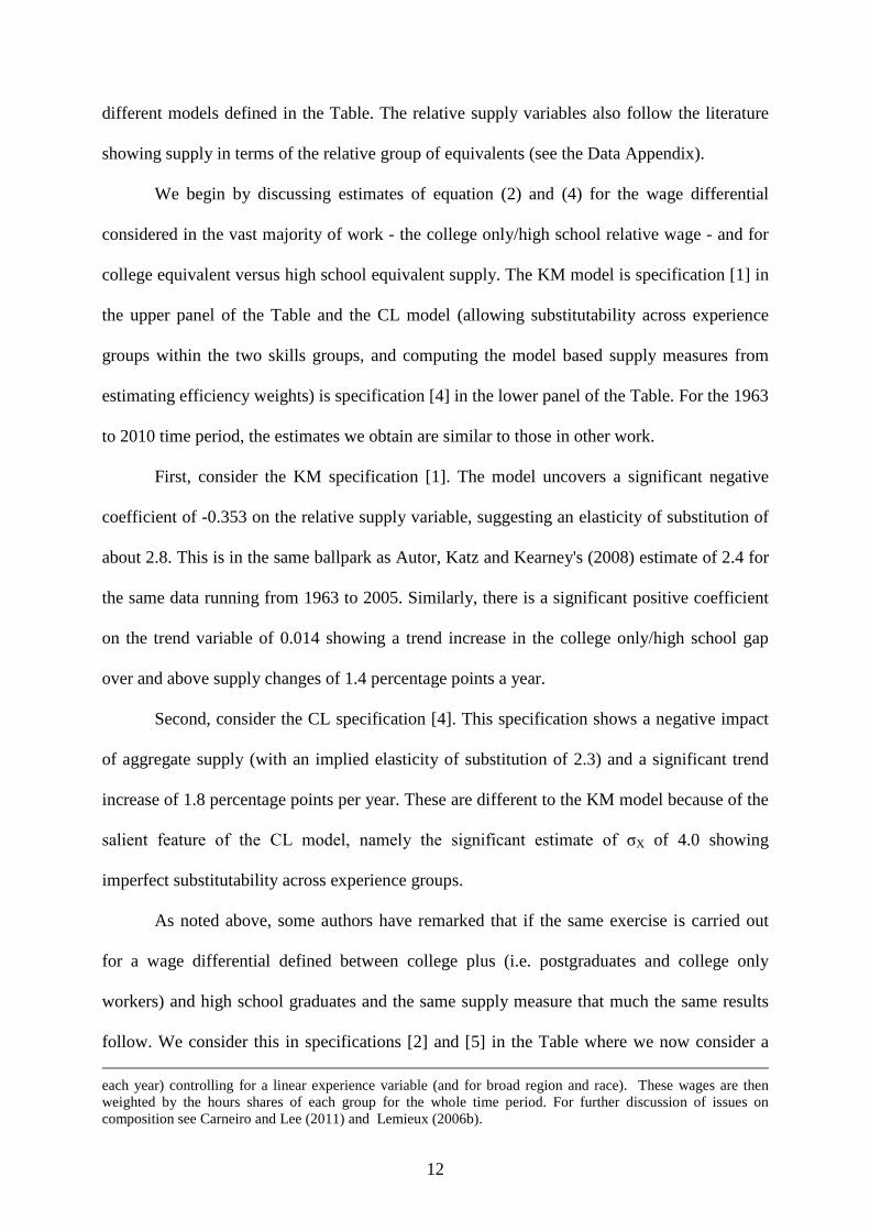
As with the Katz-Murphy model, we can again make the technological parameters a

function of the linear time trend so that the estimating equation becomes the following:

jt2t

1t

2jt

1jt3

2t

1t210

2jt

1jt

E

Elog

E

Elog

E

Elogt

W

Wlog v

(4)

where the coefficient on the trend δ1 indicates the relative demand shift over and above

supply changes, δ2 = -1/σE, δ3 = -1/σX and v is an error term.13

Estimates of Supply-Demand Models

We present estimates of the Katz-Murphy (KM) and Card-Lemieux (CL)

specifications (respectively equations (2) and (4) above) in Table 3. Our time series is too

short to undertake a rigorous analysis for the GB data, so this part of the analysis only

considers the US. The dependent variable (as in other papers in the literature) is a

composition-adjusted relative wage14, with the relevant relative wage under consideration in

13 In practice, the equation from the two-level nested CES model is estimated as a two step procedure. First, thecoefficient δ3 can be estimated from regressions of the relative wages of different experience/age groups to theirrelative supplies to derive a first estimate of σX and a set of efficiency parameters (the β1's and β2's in the CESsub-aggregates) can be obtained for each education group from a regression of wages on supply includingexperience/age fixed effects and time dummies. Given these, one can then compute E1t and E2t to obtain a modelbased estimate of aggregate supply. See Card and Lemieux (2001) for more detail.14 The composition adjustment is described in the Data Appendix. Essentially we take a similar approach toAutor, Katz and Kearney (2008) and estimate predicted fixed weight wage differentials from annual wageregressions disaggregated by gender and the four potential experience groups (i.e. eight separate regressions for

12

different models defined in the Table. The relative supply variables also follow the literature

showing supply in terms of the relative group of equivalents (see the Data Appendix).

We begin by discussing estimates of equation (2) and (4) for the wage differential

considered in the vast majority of work - the college only/high school relative wage - and for

college equivalent versus high school equivalent supply. The KM model is specification [1] in

the upper panel of the Table and the CL model (allowing substitutability across experience

groups within the two skills groups, and computing the model based supply measures from

estimating efficiency weights) is specification [4] in the lower panel of the Table. For the 1963

to 2010 time period, the estimates we obtain are similar to those in other work.

First, consider the KM specification [1]. The model uncovers a significant negative

coefficient of -0.353 on the relative supply variable, suggesting an elasticity of substitution of

about 2.8. This is in the same ballpark as Autor, Katz and Kearney's (2008) estimate of 2.4 for

the same data running from 1963 to 2005. Similarly, there is a significant positive coefficient

on the trend variable of 0.014 showing a trend increase in the college only/high school gap

over and above supply changes of 1.4 percentage points a year.

Second, consider the CL specification [4]. This specification shows a negative impact

of aggregate supply (with an implied elasticity of substitution of 2.3) and a significant trend

increase of 1.8 percentage points per year. These are different to the KM model because of the

salient feature of the CL model, namely the significant estimate of σX of 4.0 showing

imperfect substitutability across experience groups.

As noted above, some authors have remarked that if the same exercise is carried out

for a wage differential defined between college plus (i.e. postgraduates and college only

workers) and high school graduates and the same supply measure that much the same results

follow. We consider this in specifications [2] and [5] in the Table where we now consider a

each year) controlling for a linear experience variable (and for broad region and race). These wages are thenweighted by the hours shares of each group for the whole time period. For further discussion of issues oncomposition see Carneiro and Lee (2011) and Lemieux (2006b).

13

relative wage as the postgraduate to high school graduate wage. If the college plus group is

homogenous (and the postgraduates and college only workers can be thought of as perfect

substitutes) then one should see the same estimates as in specifications [1] and [4].

Whilst qualitatively similar (i.e. supply depresses wage differentials and there is a

significant trend increase in relative wages over and above supply) the magnitudes of the

estimated effects turn out to be rather different. In the KM model, the implied elasticity of

substitution is now 2.2 (as compared to the 2.8 above for college only), not surprisingly

showing less substitutability of postgraduates with high school graduates. Moreover, the trend

coefficient is around 50 percent higher at 0.020 compared to 0.014. Both these

postgraduate/college only gaps are statistically significant. The same pattern emerges for the

CL model. In specification [5], the estimated impact of aggregate relative supply on relative

wages is more marked than in specification [4], suggesting a slightly lower substitution

elasticity of 1.9 (as compared to 2.3). In addition, the trend coefficient is larger (at 0.024 vis-à-

vis 0.018).

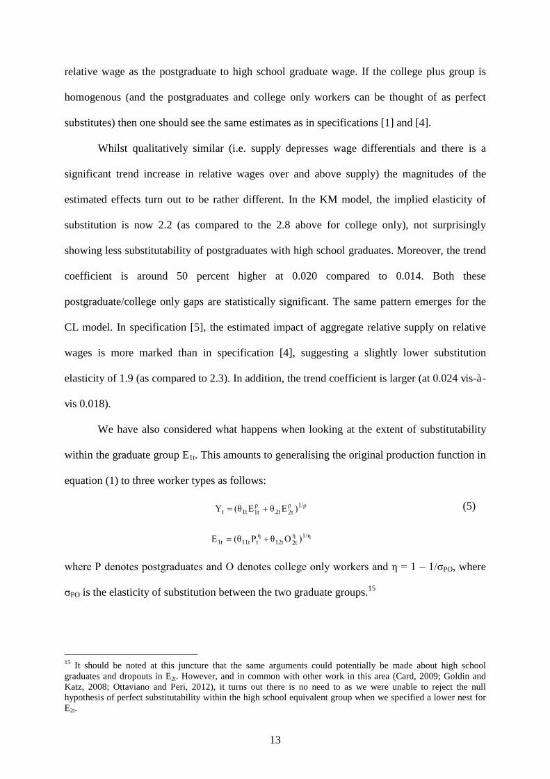
We have also considered what happens when looking at the extent of substitutability

within the graduate group E1t. This amounts to generalising the original production function in

equation (1) to three worker types as follows:

1/ρρ2t2t

ρ1t1tt )EθE(θY

1/ηη2t12t

ηt11t1t )OθP(θE

(5)

where P denotes postgraduates and O denotes college only workers and η = 1 – 1/σPO, where

σPO is the elasticity of substitution between the two graduate groups.15

15 It should be noted at this juncture that the same arguments could potentially be made about high schoolgraduates and dropouts in E2t. However, and in common with other work in this area (Card, 2009; Goldin andKatz, 2008; Ottaviano and Peri, 2012), it turns out there is no need to as we were unable to reject the nullhypothesis of perfect substitutability within the high school equivalent group when we specified a lower nest forE2t.

14

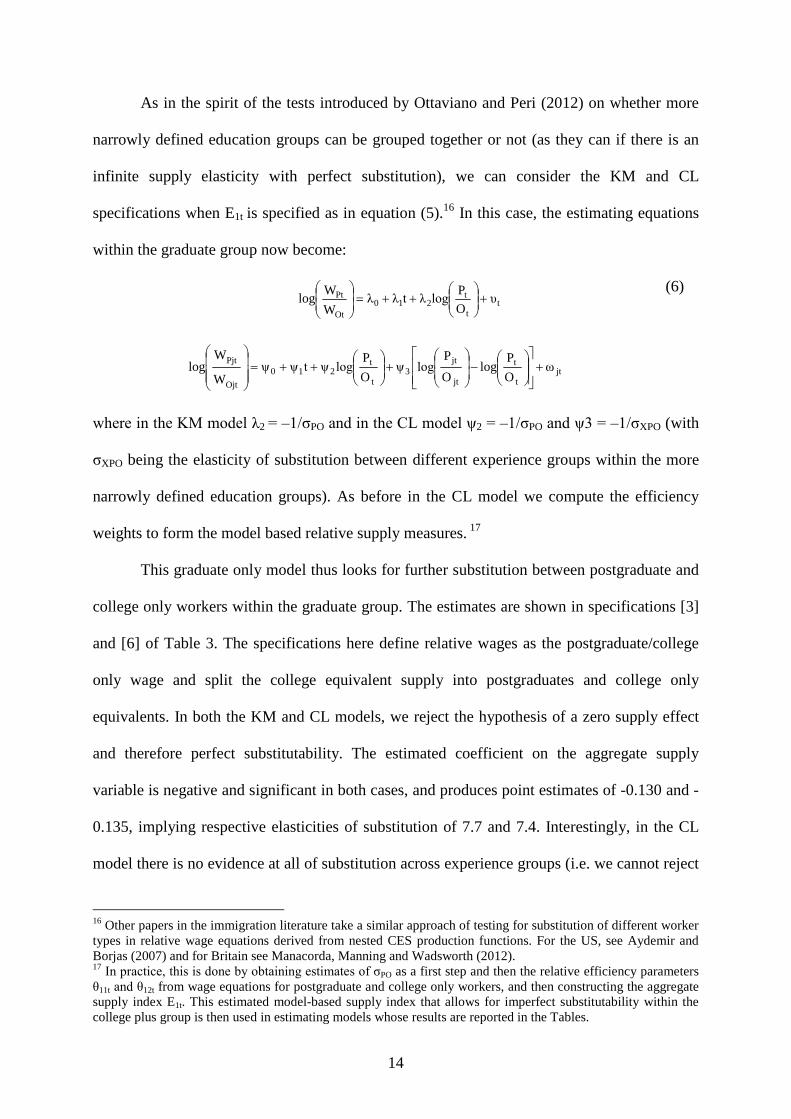
As in the spirit of the tests introduced by Ottaviano and Peri (2012) on whether more

narrowly defined education groups can be grouped together or not (as they can if there is an

infinite supply elasticity with perfect substitution), we can consider the KM and CL

specifications when E1t is specified as in equation (5).16 In this case, the estimating equations

within the graduate group now become:

tt

t210

Ot

Pt υO

Plogλ t λ λ

W

Wlog

jtt

t

jt

jt3

t

t210

Ojt

Pjtω

O

Plog

O

Plogψ

O

Plogψ t ψ ψ

W

Wlog

(6)

where in the KM model λ2 = –1/σPO and in the CL model ψ2 = –1/σPO and ψ3 = –1/σXPO (with

σXPO being the elasticity of substitution between different experience groups within the more

narrowly defined education groups). As before in the CL model we compute the efficiency

weights to form the model based relative supply measures. 17

This graduate only model thus looks for further substitution between postgraduate and

college only workers within the graduate group. The estimates are shown in specifications [3]

and [6] of Table 3. The specifications here define relative wages as the postgraduate/college

only wage and split the college equivalent supply into postgraduates and college only

equivalents. In both the KM and CL models, we reject the hypothesis of a zero supply effect

and therefore perfect substitutability. The estimated coefficient on the aggregate supply

variable is negative and significant in both cases, and produces point estimates of -0.130 and -

0.135, implying respective elasticities of substitution of 7.7 and 7.4. Interestingly, in the CL

model there is no evidence at all of substitution across experience groups (i.e. we cannot reject

16 Other papers in the immigration literature take a similar approach of testing for substitution of different workertypes in relative wage equations derived from nested CES production functions. For the US, see Aydemir andBorjas (2007) and for Britain see Manacorda, Manning and Wadsworth (2012).17 In practice, this is done by obtaining estimates of σPO as a first step and then the relative efficiency parametersθ11t and θ12t from wage equations for postgraduate and college only workers, and then constructing the aggregatesupply index E1t. This estimated model-based supply index that allows for imperfect substitutability within thecollege plus group is then used in estimating models whose results are reported in the Tables.

15

the hypothesis that 1/σXPO = 0). This is the reason why the KM and CL models yield very

close substitution elasticities.

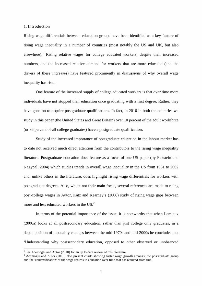
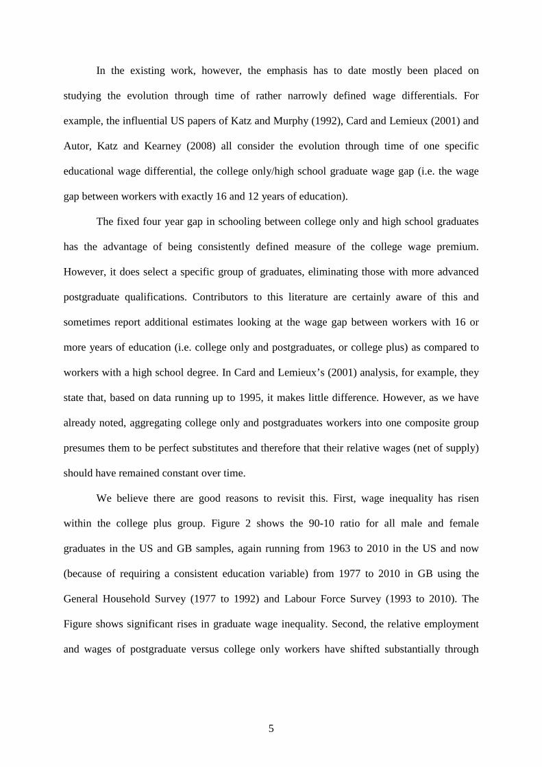
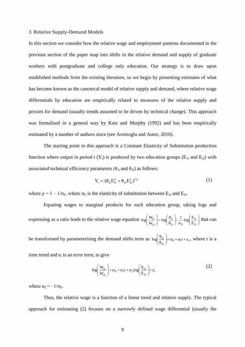
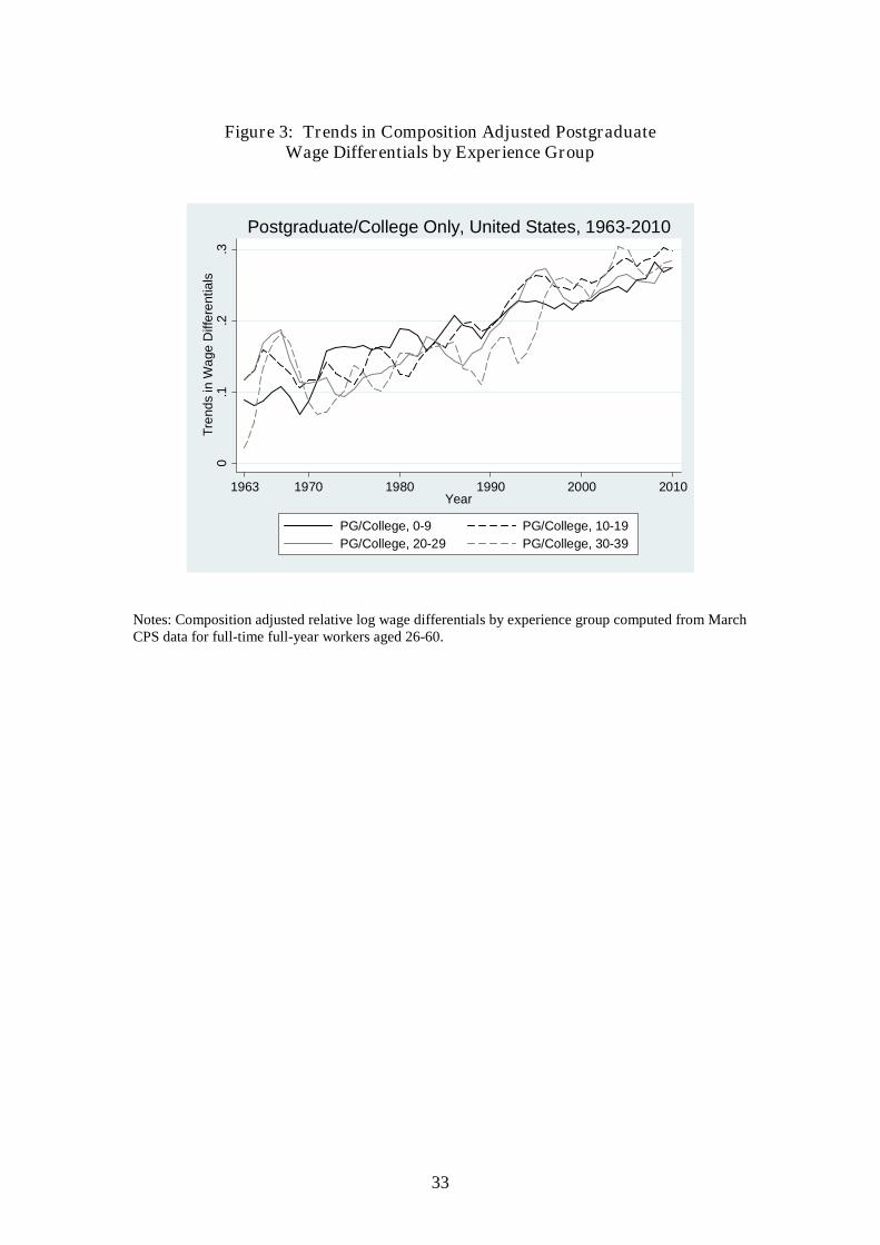
Another way to note the similarity of the KM and CL estimates in the

postgraduate/college only comparison is to note that relative wages do not show strongly

different patterns over time for low versus high experience (or younger versus older) workers.

This is made clear by looking at Figure 3, which shows trends in the composition adjusted

postgraduate/college only relative wage across higher and lower experience groups.

The models also show the importance of relative demand shifts in favour of

postgraduates as compared to college only workers. The significant coefficient on the trend

variable shows an annual increase in relative wages, over and above supply changes, of 0.5

percentage points per year or cumulatively a very sizable 24 percentage points increase over

the full 48 years. Demand driven increases in postgraduate/college only wage gaps have

therefore been an important aspect of rising within-group inequality amongst graduates.18

The Skills That Make Postgraduates More in Demand Than College Only Graduates

An obvious question that emerges is to ask what are the skills possessed by

postgraduates that make them imperfect substitutes for college only workers? Data is sparse

on this, but we can shed light on the question by looking at the British 2006 Skills Survey that

contains information on education levels of workers, but also on their specific skills in terms

of the job tasks done by workers.

Table 4 shows postgraduate/college only differences in cognitive skills, problem

solving skills, people skills, firm-specific skills, the tasks they use computers for and the

18 In an earlier version of this paper, we explored different ways of modelling the demand shift in the KM and CLmodels. Some authors (Autor, Katz and Kearney, 2008; Goldin and Katz, 2008) have addressed this issue bylooking at trend non-linearities or trend breaks. We took a different approach, replacing the linear trend with atechnology proxy, the log of the real ICT capital stock. For our interest in postgraduates, both the KM and CLmodels incorporating the real ICT capital variable corroborate the findings from before and, if anything, turnedout to be stronger. The Ottaviano-Peri (2012) type test in specifications [3] and [6] more strongly rejects thehypothesis of constant wage evolutions for postgraduates and college only graduates. For the KM and CL modelsthe estimated coefficients (standard errors) on the supply variable were -0.155 (0.071) and -0.158 (0.057).Moreover, the strong and significant coefficient on the real ICT measure suggested that, over time, technologydriven demand has been shifting strongly in favour of postgraduate relative to college only workers.

16

routineness of their job. Most of the numbers in the Table (with the exception of the

proportions using computers) are based on a scale of 1-5 (5 being highest) from questions on

task performance asking 'How important is this task in your current job?', with 1 denoting 'not

at all important', 2 'not very important', 3 'fairly important', 4 'very important' and 5 'essential'.

It is clear that both sets of graduates do jobs with high skill and job task requirements.

However, in almost all cases the levels are higher (and significantly so) for postgraduates. For

example, postgraduates have higher numeracy levels (especially advanced numeracy), higher

levels of analysing complex problems and specialist knowledge or understanding.19 The

computer usage breakdowns are also interesting, showing clearly that postgraduates and

college only workers have high levels of computer usage, but that using computers to perform

complex tasks is markedly higher amongst the postgraduate group.

We view the Table 4 material as confirming that postgraduates do possess different

skills and do jobs involving different (usually more complex) tasks than college only workers.

This is further evidence of them being imperfect substitutes and, as they seem to possess

higher skill levels, is in line with the fact that relative demand has shifted faster in favour of

the postgraduate group within the group of all college graduates.20 As such, this is an

important aspect of rising wage inequality amongst college graduates.

Which Occupations do Postgraduates and College Only Graduates Work in?

We have also looked at another dimension by which postgraduate and college only

workers differ and that relates to their imperfect substitutability by looking in which

occupations they are employed. Table 5 shows the top ten occupations in terms of their share

19 These are all skills that are becoming more highly valued in the labour market through time (see Green, 2012).20 They are also in line with the task continuum model that Acemoglu and Autor (2010) introduce in the contextof their discussion of the shortcomings of the canonical model. They state that the canonical model is a usefuland powerful way to model how the supply and demand for skills have affected wage differentials through time,but argue for generalising it in terms of a task-based model with an allocation of skills to tasks and in which newtechnology substitutes for workers doing certain (more routine) tasks. In terms of the task continuum in theirmodel, we view our evidence as illustrating that postgraduates do tasks at the top end of the task continuum andthus are not substitutable by computers or other new technologies. This seems very consistent with our resultsshowing postgraduates doing tasks that are more advanced and performing better in the labour market thancollege only workers and with their higher complementarity with computers.

17

in employment for college only and postgraduate workers in 2010 for the US (in the upper

panel) and for GB (in the lower panel).

There are several interesting features of the top ten occupations of these three groups

of workers. First, other than in the education sector, the top ten tend to be different

occupations in both countries. Second, whilst the occupational categories are not quite the

same across countries, there are some clear similarities. Third, the postgraduate occupations

are more segregated than the college only. For postgraduates, in both countries the top ten (in

the US out of 497 occupations, and for GB out of 353 occupations) account for just over 40

percent. The college only distribution is more dispersed, with the top ten for more like a

quarter.21 It is evident that college only workers are spread more widely across the

occupational structure and the occupational distribution of postgraduates is more segregated.

The differences in the occupational structure of employment for the postgraduate

group vis-à-vis college only graduates offers additional corroborative evidence relevant to our

earlier findings of less than perfect substitution and in the trend differences in relative wages

net of relative supply between the postgraduate and college only group.

Thus, overall, we have found evidence of imperfect substitutability of the two different

groups of graduates. As a consequence, the (implicit) view that postgraduates are just more

productive versions of college only workers does not rest well with these findings. The other

key result from the supply and demand modes is that demand has shifted significantly in

favour of postgraduates within the graduate group and that this has played an important role in

raising wage inequality amongst college graduates. In the next section of the paper, we probe

this further, looking at what has driven this increased relative demand for postgraduates by

studying differences in technology-skill complementarities for postgraduate as compared to

college only workers.

21 Benson (2011) considers the spatial distribution of occupations in the US by education group. Whilst not themain focus of his analysis, he shows the occupational structure of postgraduates to be more segregated than forcollege only workers (and indeed for the rest of the labour force).

18

4. Technology-Skill Complementarities and Labour Market Polarization

We now shift the focus to ask why the demand for postgraduate and college only workers has

been different. Again utilising the approaches used in existing work that does not distinguish

between the two different groups of graduates, we study correlations between temporal shifts

in relative demand and observable technology measure and look at whether one can identify

cross-country similarities in the observed patterns of change.

Industry Computerization and Skill Demand

A large body of research connects relative demand shifts underpinning increased wage

inequality to observable measures of technology, usually relating the two through industry-

level regressions.22 This work reveals that technology measures like R&D, innovation and

computerization are positively correlated with long run secular increases in the demand for

more educated workers, thus showing important technology-skill complementarities.

For our purposes, it is interesting to ask whether technology-skill complementarities

are different for postgraduate and college only workers. We explore this question by

estimating the following long run within-industry relationship between changes in relative

labour demand of different education groups, S, and changes in computer use, C, as:

1ejtωjΔC1eγ1eλejtΔS (7)

where ejτSejtSejtΔS is change in the employment share for education group e in industry j

between years τ and t (in the US between 1989 and 2008, and for GB between 1996 and 2008)

and ΔCj is the change in the proportion of workers in industry j using a computer at work

between 1984 and 2003 for the US (from the October Current Population Survey

22 The seminal article is Berman, Bound and Griliches (1994) which related changes in the demand for skilledlabour in US manufacturing industries to measures of R&D and computer investment. Autor, Katz and Krueger(1998) study connections with industry computerization, and Berman, Bound and Machin (1998) and Machin andVan Reenen (1998) offer cross-country comparisons based on the same industries across countries. This by nowsizable literature is reviewed in Katz and Autor (1999).

19

Supplements) and between 1992 and 2006 for GB (from the 1992 Employment in Britain and

the 2006 Skills Survey).

To evaluate the longer run impact of computer use (since the initial introduction of

computers in the PC era) we also augment equation (7) by the initial level of computer usage

(in 1984 for the US and 1992 for GB) as follows:

2ejtωinitialjC2ejΔC2eγ2eλejtΔS (8)

where initialjC is the initial computer use proportion (measured in 1984 for the US and 1992

for GB). The inclusion of this variable can be thought one in one of two (related) ways. First,

by holding constant the initial stock of computers, its inclusion implies the estimated

coefficient on ΔCj picks up effects of the change in computer use from then. Second, under the

assumption that in earlier periods (say back in the 1960s or 1970s) the computer use

proportion was essentially zero, the variable itself can be viewed as picking up growth in

computer use effects up to the time period in which the variable is measured.

US Results

Estimates of equation (7) and (8) are reported for five education shares in Table 6. As

per the main focus of this paper, the five education groups generalise on the four used in

earlier work by breaking down the college plus group into postgraduates and college only

workers.23 The upper panel of the Table focuses on the US, the lower panel on GB and in each

case the two specifications showing the estimates of 1eγ from equation (7) and 2eγ and 2e

from equation (8) are shown.

Considering first the US results, specification [1] in Table 6 uncovers different

connections between the postgraduate and college only changes in employment shares and

23 In their US study, Autor, Katz and Krueger (1998) look at four education groups: college, some college, highschool graduates and less than high school. Given our focus on heterogeneity in the college group, we split thatinto postgraduates and college only, so as to look at five groups. We also study five (broadly comparable groups)in the GB data: postgraduates, college only, intermediate 1, intermediate 2 and no qualifications. (See theAppendix for more detail on the precise definitions used.)

20

changes in computer use. Indeed, the positive connection reported in earlier work (e.g. Autor,

Katz and Krueger, 1998) is only present for the postgraduate group. It seems that the

connections between industry changes in skill demand and changes in computerization are not

neutral across the two groups of college graduates.

Results for the three other education groups (some college, high school graduates and

high school dropouts), show much the same pattern as seen in earlier work, where the main

losers from increased computerization are the high school graduates (not the dropouts).24 This,

of course, is consistent with computerization playing a significant role in the polarization of

skill demand (where jobs were hollowed out and/or relative wages deteriorated in the middle

part of the education distribution).25 We will return to discuss the role of postgraduates in

these polarization patterns below.

The second US specification [2] in Table 6 shows estimates of equation (6) which

additionally include the 1984 computer use proportion. This sheds more light on what has

been going on within the graduate group. The change in the postgraduate employment share

is significantly related to both the 1984 to 2003 increases in industry computerization and to

the 1984 level. On the other hand, the change in the college only wage bill share is

insignificantly related to the 1984 to 2003 change and positively and significantly only to the

initial 1984 level.

Thus, the initial influx of computers to industries benefited both groups, but thereafter

the group of graduates who benefited was confined to those with a postgraduate qualification.

This paints a rather different picture as to who benefited most from the computer revolution.

It seems initially that labour demand shifted in favour of all graduates, but as time progressed

24 Like Autor, Katz and Kreuger (1998), we obtain a positive significant coefficient on computerization in thehigh school dropouts share equation. This ultimately arises, as Autor, Katz and Krueger clearly state, because thehigh school dropout share becomes very small in many industries in the latter period of the sample. As our dataextend further, this is even more the case for our analysis, but like them, controlling for the initial (lagged)education share does ameliorate this, although our interpretation of the computer effects as reflecting polarizationwith the bigger negative effects for the intermediate education groups remains robust to this.25 Our results are very much in line with Michaels, Natraj and Van Reenen (2013) who report cross-countryevidence connecting polarization to computerization.

21

labour demand tilted more in favour of postgraduates. This suggests that more recently

postgraduates possess skills that make them more complementary to computers, a point we

return to towards the end of this section where we look directly at differences in the skills of

postgraduate and college only workers.

It is worth benchmarking the within-college group differences for postgraduates and

college only with the earlier work where the overall college share (i.e. the sum of the two

shares) was used as dependent variable. If we put them together in one college plus group as

in the earlier work, we obtain a coefficient (and associated standard error) of 0.131 (0.031) on

the 1984 to 2003 ΔCj variable and of 0.010 (0.001) on the 1984 initialjC variable. Therefore, like

the earlier work, there is indeed a strong connection between changes in college plus

employment shares and computers, but our findings highlight that it is one characterised by

non-neutrality of technology-skill complementarity across the postgraduate and college only

groups. Put differently, postgraduates more highly complement computers as compared to

college only workers and thus have benefited more from their spread.

GB Results

The lower panel of Table 6 gives the GB results. Consider specification [3] first. As

with the US findings, we find non-neutrality amongst the two groups of graduates. We obtain

a significant positive coefficient on the postgraduate variable and an insignificant (positive)

one on the college only variable. The same is true in specification [4] when the initial

computer usage variable (measured in 1992) is included. Here though, it is evident that there

are strong and significant connections between changes in the postgraduate employment share

and both changes in industry computerization and the 1992 level of computer usage. On the

other hand, connections with the college only share are not statistically significant.

For the other three education groups, the results also confirm that the British labour

market was also characterised by polarization connected to industry computerization and its

22

associations with changes in the relative wages and employment of workers with different

education levels. The hollowing out of the middle is seen in the results reported in the Table

where the intermediate qualification groups fare worst, whilst those at each end of the

education spectrum (the postgraduates at the top and the no qualifications group at the bottom)

have the best outcomes in relative terms.

Sub-Period Analysis and Complex/Basic Computer Use

The notion that increased computer usage acts as a measure of new technology over

the whole time period we consider also requires some discussion (see Beaudry, Doms and

Lewis, 2010, who critically appraise the extent to which the widespread use of personal

computers reflects a technological revolution). This is a potentially important aspect of our

analysis in that we look at changes in computer usage between 1984 and 2003 as, by 2003, in

some industries the percentage of workers using a computer is high. This possible near

reaching of a ceiling, of course, shows the need to control for initial levels of computer usage

in the regressions. It also raises the question of whether changes in a simple headcount

measure of any computer use at work adequately reflect technological change.

We consider this question in two ways for the US analysis (sample size issues

precluded a similar analysis being undertaken for GB). First, we break down the analysis into

two sub-periods. These are dictated by the availability of computer usage data in the CPS in

the October supplements of 1984, 1993 and 2003. We thus look at changes in employment

shares between 1998 and 2008 and how they relate to changes in computer usage between

1993 and 2003, and perform the same sub-period split for changes in employment shares

between 1989 and 1998 with computer use changes measured from 1984 to 1993.26

26 The second period closely approximates the time period studied by Autor, Katz and Krueger (1998). Autor,Katz and Krueger report an estimated coefficient (standard error) of 0.152 (0.025) on the computer use variablein a regression of changes in college plus employment shares between 1979 and 1993 on the 1984 to 1993 changein computer usage for 191 US industries. Running the same regression (i.e. not including the initial level ofcomputer usage) on our 215 industries for the change in college plus employment shares between 1989 and 1998we obtain a very similar estimate of 0.144 (0.026) on the 1984 to 1993 change in computer use variable. For this

23

Estimates of equation (6) are reported in specifications [1] and [2] of Table 7 for these

two sub-periods. The analysis corroborates the earlier findings where there is a stronger

computerization effect for postgraduates than for college only workers. A closer inspection of

the results does, however, reveal that this more true of the first sub-period (in specification

[1]). In the second sub-period (specification [2]) the postgraduate and college only

computerization effects are more similar.

To further probe this, the second way we consider the usefulness of the computer

usage data to measure technological change is by breaking down the computerization measure

into whether the computer is used for complex or basic tasks. For the second period of data we

can do this since the 1993 and 2003 computer use supplements in the CPS report whether

computers are used for more complex tasks like programming as well as for a variety of other

more basic purposes (see the Data Appendix for more detail). We therefore define complex

use as computer programming and basic use as all other computer use.

Specification [3] of Table 7 reports the results. Changes in complex computer usage

are strongly associated with the increased demand for postgraduates. Both the change and the

initial level of complex computer usage have a positive and significant impact on the change

in the postgraduate share of employment. The same is not true of the college only group,

where it is changes in basic computer usage that are significantly related to increased

employment of this group of workers.

Thus it seems that whilst increased computer usage over time could in part reflect the

widespread use of computers as becoming a general purpose technology, once the complexity

of tasks used for by computers is considered, this has been an important factor in explaining

the differential demand for postgraduate vis-à-vis college only workers. Therefore in more

technologically advanced industries, a higher complementarity of postgraduates with

specification, considering postgraduate and college only shares separately produces a coefficient (standard error)of 0.087 (0.015) on the change in computer use variable in a change in postgraduate share equation and of 0.057(0.023) in a change in college only share equation.

24

computers used for complex tasks has meant the demand for postgraduates has increased at a

faster rate than demand for college only workers over the last twenty five years.27

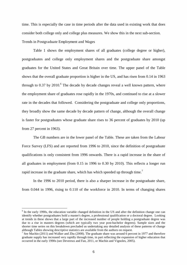
Cross-Country Correlations

The fact that we have comparable data in two countries means we can further

investigate the relative demand shifts in favour of postgraduates by asking the question

whether one sees bigger shifts occurring in the same industries in the two countries. Earlier

work on shifts in relative demand by Berman, Bound and Machin (1998) took this very

approach to show that there were cross-country commonalities in shifts in industry skill

demand in advanced countries in the 1970s and 1980s, as would be predicted by the skill-

biased technological change hypothesis.

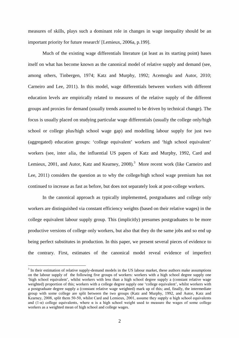
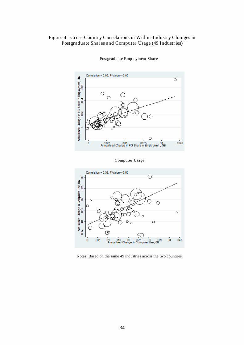
Table 8 shows US-GB cross-country correlations of industry levels and changes in

employment shares and computerization. These are computed for the same 49 (roughly 2-

digit) industries for the two countries. The levels are all strongly correlated as shown in the

first column. However, our main interest is in the correlations in the within-industry changes

as reported in the second column. These are also strongly correlated for employment shares

and for computerization. It seems that it is the same industries in the two countries that had

faster increases in computer usage and, at the same time, shifts in relative demand towards

postgraduates. The correlations are strong (with p-values showing statistical significance

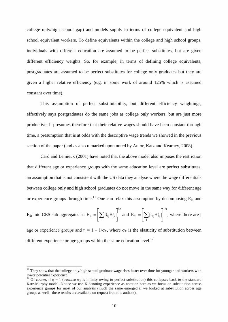
levels of better than 1 percent in all cases). Figure 4 plots US versus GB changes in

postgraduate employment shares and changes in computer usage and fits a regression line

through them, showing these strong cross-country correlations.

27 In earlier versions of this paper (e.g. Lindley and Machin, 2011) we also looked at cost share equations, albeitimplementing this analysis for a reduced number and more highly aggregated set of US industries (52) owing tothe need for capital and output data. The findings from them were strongly supportive of the pattern seen in therelative labour demand equations. Industries with more ICT investment saw faster increases in wage bill sharesfor postgraduates than for college only workers, which is indicative of non-neutrality between the two groups ofcollege graduates. There is also significant hollowing out in the middle part of the distribution with some collegeand high school graduates faring worst. These results are available on request from the authors.

25

Labour Market Polarization

As has already been noted, more recent work analysing the period of rising labour

market inequality we study has pinpointed increased job polarization – with relatively fast job

growth at the top and bottom end of the skill distribution, coupled with job falls in the middle -

as a key aspect of changing employment and wage structures. Empirical researchers have

studied how this has interacted with technology and the tasks that workers perform in their

jobs. In particular, the notion that middle skill jobs have been disproportionately lost as the job

distribution has hollowed out in the middle has received significant attention.

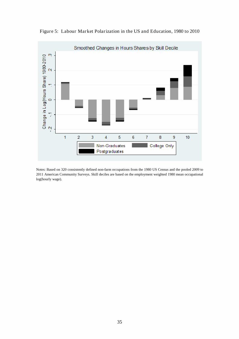
We are interested how the increased demand for postgraduates can fit in to this

framework. In Figure 5 we therefore reproduce the pattern of labour market polarization that

has been identified in US data (see Autor and Dorn, 2013, or Lindley and Machin, 2013) using

US Census and American Community Survey data between 1980 and 2010. The horizontal

axis of Figure 1 orders 1980 occupations from lowest to highest wage then shows the growth

in hours at each decile of that initial skill distribution. The growth in hours is defined in

relative terms so that a number above zero represents relative growth and a number below zero

represents negative growth. A clear pattern of hours growth at the top end emerges, together

with a hollowing out of the middle, but also positive growth at the bottom end in low wage

jobs.

In Figure 5 we have also broken down the patterns of relative growth by three

education groups: it shows hours growth of postgraduate (the black bar), college only (the

dark grey bar) and less then college workers (the light grey bar) in each decile (which sum to

the total). The Figure makes it very clear that the bulk of the hollowing out in the middle and

the growth of low wage service jobs at the bottom is from changing job prospects of workers

with less than a college education. At the top, however, the college graduates do well, with

postgraduate job growth very strong in the top decile higher skill jobs. In fact the contribution

26

of postgraduates to increased polarization at the top is stronger than for college only workers.

The latter group are also affected a little in the hollowed out middle deciles. This is in line

with the observation of Beaudry, Green and Sand (2013) who we have already noted

demonstrate deterioration in the relative demand for college only workers in the last decade of

the three decades we study. Overall, it seems that postgraduate job growth is stronger than

college only job growth in relatively high skilled jobs. This contribution to increased labour

market polarization is consistent with our earlier findings that relative demand has been

shifting more rapidly for postgraduates owing to their superior skills and ability to use new

technologies in the tasks required for high end jobs in modern workplaces.

5. Conclusions

In this paper, we present new evidence on how the changing education structure of the

workforce has contributed to rising wage inequality in the United States and Great Britain.

Our main focus is on increasing divergences within the group of workers who have been to

university. We document that there have been increases through time in the number of

workers with a postgraduate qualification. We show that, at the same time as this increase in

their relative supply, their relative wages have strongly risen as compared to workers with

only a college degree.

Consideration of shifts in their demand and supply uncovers trend increases in relative

demand for postgraduates that are a key driver of increasing within-graduate inequality. In line

with these shifts in relative demand, we report various pieces of evidence in line with the

notion that postgraduate workers and college only workers are different, in that they are not

perfect substitutes, they possess skills that have a higher value in the labour market and that

they work in different occupations.

27

The relative demand shifts in favour of workers with postgraduate qualifications are

strongly correlated with technical change as measured by computer usage and investment. It

turns out that, in the period when computers have massively diffused into workplaces,

postgraduates more highly complement computers as compared to college only workers and

thus have benefited more from their spread. This has been an important driver of rising wage

inequality amongst graduates over time as the presence of postgraduates in the workplace has

grown in importance. Their strong employment growth in high skill jobs also plays an

important role in accounting for labour market polarization at the top end of the skill

distribution.

Before concluding, it is worth noting that in this paper where necessary we choose to

focus on well established empirical approaches that have been used in prior work in the area to

show that there have different patterns of change in labour market outcomes for postgraduates

and college only workers. We do this deliberately so as not to confuse differences in

modelling approach with our findings that postgraduate and college only workers need to be

separated out in relative supply-demand models and in studies of the impact of

computerization as skill-biased demand shocks.

And last, of course, the findings of this paper do then naturally open up other channels

for future research. One important question is to better understand why some graduates have

been feeling the need to distinguish themselves from college only workers by acquiring

postgraduate qualifications. A second is to consider gender differences since women's relative

supply has increased faster than men's as more women have gone to college. A third is to

study the implications for universities of the changing balance between undergraduate and

postgraduate education. Finally, looking at whether evidence of rising graduate wage

inequality driven by higher labour market rewards for postgraduates is a feature of changing

wage structures in other countries is an important avenue for future research.

28

References

Acemoglu, D. and D. Autor (2010) Skills, Tasks and Technologies: Implications forEmployment and Earnings, in Ashenfelter, O. and D. Card (eds.) Handbook of LaborEconomics Volume 4, Amsterdam: Elsevier.

Autor, D. and D. Dorn (2013) The Growth of Low Skill Service Jobs and the Polarization ofthe US Labor Market, American Economic Review, 103, 1553-97.

Autor, D., L. Katz and A. Krueger (1998) Computing Inequality, Quarterly Journal ofEconomics, 113, 1169-1213.

Autor, D., L. Katz, and M. Kearney (2008) Trends in U.S. Wage Inequality: Re-Assessing theRevisionists, Review of Economics and Statistics, 90 300-323.

Autor, D., F. Levy and R. Murnane (2003) The Skill Content of Recent TechnologicalChange: An Empirical Investigation, Quarterly Journal of Economics, 118, 1279-1333.

Aydemir, A. and G. Borjas (2007) Cross-Country Variation in the Impact of InternationalMigration: Canada, Mexico, and the United States, Journal of the European EconomicAssociation, 5, 663-708.

Beaudry, P., M. Doms and E. Lewis (2010) Should the Personal Computer Be Considered aTechnological Revolution? Evidence from U.S. Metropolitan Areas, Journal ofPolitical Economy, 118, 988-1036.

Beaudry, P., D. Green and B. Sand (2013) The Great Reversal in the Demand for Skill andCognitive Tasks, National Bureau of Economic Research Working Paper 18901.

Berman, E., J. Bound and Z. Griliches (1994) Changes in the Demand for Skilled LaborWithin U.S. Manufacturing Industries: Evidence from the Annual Survey ofManufacturing, Quarterly Journal of Economics, 109, 367–98.

Berman, E., J. Bound and S. Machin (1998) Implications of Skill-Biased TechnologicalChange: International Evidence, Quarterly Journal of Economics, 113, 1245-1280.

Benson, A. (2011) A Theory of Dual Job Search and Sex-Based Occupational Clustering, MITmimeo.

Card, D. (2009) Immigration and Inequality, American Economic Review, 99, 1-21.

Card, D. and T. Lemieux (2001) Can Falling Supply Explain the Rising Return to College forYounger Men? A Cohort-Based Analysis, Quarterly Journal of Economics, 116, 705-46.

Carneiro, P. and S. Lee (2011) Trends in Quality-Adjusted Skill Premia in the United States,1960-2000, American Economic Review, 101, 2309-49.

Devereux, P. and W. Fan (2011) Earnings Returns to the British Education Expansion,Economics of Education Review, 30, 1153-66.

29

Eckstein, Z. and E. Nagypal (2004) The Evolution of US Earnings Inequality: 1961-2002,Federal Reserve Bank of Minneapolis Quarterly Review, 28, 10–29

Goldin, C. and L. Katz (2008) The Race Between Education and Technology, HarvardUniversity Press.

Goos, M. and A. Manning (2007) Lousy and Lovely Jobs: The Rising Polarization of Work inBritain, Review of Economics and Statistics, 89, 118-33.

Goos, M., A. Manning and A. Salomons (2009) The Polarization of the European LaborMarket, American Economic Review, Papers and Proceedings, 99, 58-63.

Green, F. (2012) Employee Involvement, Technology and Evolution in Job Skills: A Task-Based Analysis, Industrial and Labor Relations Review, 65, 36-67.

Katz, L. and D. Autor (1999) Changes in the Wage Structure and Earnings Inequality, in O.Ashenfelter and D. Card (eds.) Handbook of Labor Economics, Volume 3, NorthHolland.

Katz, L. and K. Murphy (1992) Changes in Relative Wages, 1963-87: Supply and DemandFactors, Quarterly Journal of Economics, 107, 35-78.

Lefter, A. and B. Sand (2011) Job Polarization in the US: A Reassessment of the EvidenceFrom the 1980s and 1990s, University of St. Gallen Discussion Paper 2011-03.

Lemieux, T. (2006a) Postsecondary Education and Increasing Wage Inequality, AmericanEconomic Review, Papers and Proceedings, 96, 195-99.

Lemieux, T. (2006b) Increased Residual Wage Inequality: Composition Effects, Noisy Data orRising Demand for Skill, American Economic Review, 96, 461-98.

Lindley, J. and S. Machin (2011) Postgraduate Education and Rising Wage Inequality, IZADiscussion Paper No. 5981.

Lindley, J. and S. Machin (2013) Spatial Changes in Labour Market Inequality, Journal ofUrban Economics, forthcoming.

Machin, S. (2011) Changes in UK Wage Inequality Over the Last Forty Years, in P. Greggand J. Wadsworth (eds.) The Labour Market in Winter - The State of Working Britain2010, Oxford University Press.

Machin, S. and J. Van Reenen (1998) Technology and Changes in Skill Structure: EvidenceFrom Seven OECD countries, Quarterly Journal of Economics, 113, 1215-44.

Machin, S. and A. Vignoles (2005) What's the Good of Education?, Princeton UniversityPress.

30

Manacorda, M., A. Manning and J. Wadsworth (2012) The Impact of Immigration on theStructure of Male Wages: Theory and Evidence From Britain, Journal of the EuropeanEconomic Association, 10, 120-51.

Michaels, G. A. Natraj and J. Van Reenen (2013) Has ICT Polarized Skill Demand? Evidencefrom Eleven Countries over 25 years, Review of Economics and Statistics,forthcoming.

Ottaviano, G. and G. Peri (2012) Rethinking the Effects of Immigration on Wages, Journal ofthe European Economic Association, 10, 152-97.

Spitz-Oener, A. (2006) Technical Change, Job Tasks and Rising Educational Demands:Looking Outside the Wage Structure, Journal of Labor Economics, 24, 235-70.

Tinbergen, J. (1974) Substitution of Graduate by Other Labour, Kyklos, 27, 217-26.

Walker, I. and Y. Zhu (2008) The College Wage Premium and the Expansion of HigherEducation in the UK, Scandinavian Journal of Economics, 110, 695-709.

31

Figure 1: Trends in Overall 90-10 Wage Ratio

11.2

1.4

1.6

90

-10

Log

FT

Ea

rnin

gs

Ra

tio

1963 1970 1980 1990 2000 2010Year

Men Women

United States, 1963 to 2010

.8.9

11.1

1.2

1.3

90

-10

Log

FT

Ea

rnin

gs

Ra

tio

1975 1980 1990 2000 2010Year

Men Women

Great Britain, 1975 to 2010

Notes: US 90-10 Log(Earnings) ratios from March Current Population Surveys for income years 1963to 2010. Weekly earnings for full-time full-year workers. GB 90-10 Log(Earnings) ratios from 1975 to2010 from the New Earnings Survey/Annual Survey of Hours and Earnings. Weekly earnings for full-time workers.

32

Figure 2: Trends in 90-10 Wage Ratio For Graduates

.91.1

1.3

1.5

90

-10

Log

FT

Ea

rnin

gs

Ra

tio

1963 1970 1980 1990 2000 2010Year

Graduate Men Graduate Women

United States, 1963 to 2010

.81

1.2

1.4

90

-10

Log

FT

Ea

rnin

gs

Ra

tio

1977 1990 2000 2010Year

Graduate Men Graduate Women

Great Britain, 1977 to 2010

Notes: US 90-10 Log(Earnings) ratios from March Current Population Surveys for income years 1963to 2010. Weekly earnings for full-time full-year graduate workers. GB 90-10 Log(Earnings) ratios from1977 to 2010 from splicing together the General Household Survey (1977-1992) to the Labour ForceSurvey (1993 to 2010). Weekly earnings for full-time workers (those working 30 or more hours).

33

Figure 3: Trends in Composition Adjusted PostgraduateWage Differentials by Experience Group

0.1

.2.3

Tre

nd

sin

Wa

ge

Diffe

rentia

ls

1963 1970 1980 1990 2000 2010Year

PG/College, 0-9 PG/College, 10-19

PG/College, 20-29 PG/College, 30-39

Postgraduate/College Only, United States, 1963-2010

Notes: Composition adjusted relative log wage differentials by experience group computed from MarchCPS data for full-time full-year workers aged 26-60.

34

Figure 4: Cross-Country Correlations in Within-Industry Changes inPostgraduate Shares and Computer Usage (49 Industries)

Postgraduate Employment Shares

Computer Usage

Notes: Based on the same 49 industries across the two countries.

35

Figure 5: Labour Market Polarization in the US and Education, 1980 to 2010

Notes: Based on 320 consistently defined non-farm occupations from the 1980 US Census and the pooled 2009 to

2011 American Community Surveys. Skill deciles are based on the employment weighted 1980 mean occupational

log(hourly wage).

36

Table 1: Employment Shares by Education

United States

1963 1970 1980 1990 2000 2010

College Degree or Higher 0.137 0.158 0.238 0.277 0.316 0.370Postgraduate Degree 0.037 0.046 0.075 0.089 0.106 0.132College Degree Only 0.100 0.112 0.164 0.189 0.209 0.238Postgraduate Share 0.268 0.290 0.313 0.320 0.337 0.357

Great Britain

1996 2000 2010

College Degree or Higher 0.145 0.180 0.304Postgraduate Degree 0.044 0.057 0.110College Degree Only 0.101 0.123 0.194Postgraduate Share 0.301 0.315 0.362

Notes: Source for United States is March Current Population Surveys. Source for Great Britain is Labour Force Surveys. Employment shares are defined for people in workwith 0 to 39 years of potential experience and aged 26 to 60.

37

Table 2: Wage Differentials by Education

United States1963 1970 1980 1990 2000 2010

College Degree or Higher 0.337(0.011)

0.416(0.008)

0.384(0.007)

0.529(0.006)

0.628(0.008)

0.682(0.007)

Postgraduate Degree 0.338(0.020)

0.455(0.013)

0.470(0.010)

0.641(0.009)

0.768(0.010)

0.856(0.008)

College Degree Only 0.337(0.012)

0.402(0.009)

0.344(0.007)

0.476(0.007)

0.555(0.008)

0.583(0.007)

Postgraduate Degree Versus College Degree Only 0.001(0.021)

0.053(0.014)

0.125(0.010)

0.165(0.010)

0.214(0.011)

0.273(0.008)

Sample Size 12100 23217 29546 34944 29436 41961

Great Britain1996 2000 2010

College Degree or Higher 0.468(0.007)

0.470(0.007)

0.497(0.007)

Postgraduate Degree 0.504(0.015)

0.540(0.010)

0.579(0.010)

College Degree Only 0.451(0.011)

0.435(0.008)

0.449(0.009)

Postgraduate Degree Versus College Degree Only 0.052(0.017)

0.104(0.011)

0.130(0.011)

Sample Size 20072 36590 23964

Notes: Source for United States is March Current Population Survey. Source for Great Britain is 1996, 2000 and 2010 Labour Force Surveys. Full-time full-year workerswith 0 to 39 years of potential experience and aged 26 to 60 in the US; full-time workers with 0 to 39 years of potential experience and aged 26 to 60 in GB. Wagedifferentials relative to high school graduates in the US and intermediate qualifications in GB. Control variables included are: gender, experience, experience squared, broadregion and race (US); gender, experience, experience squared, London and white. Standard errors in parentheses.

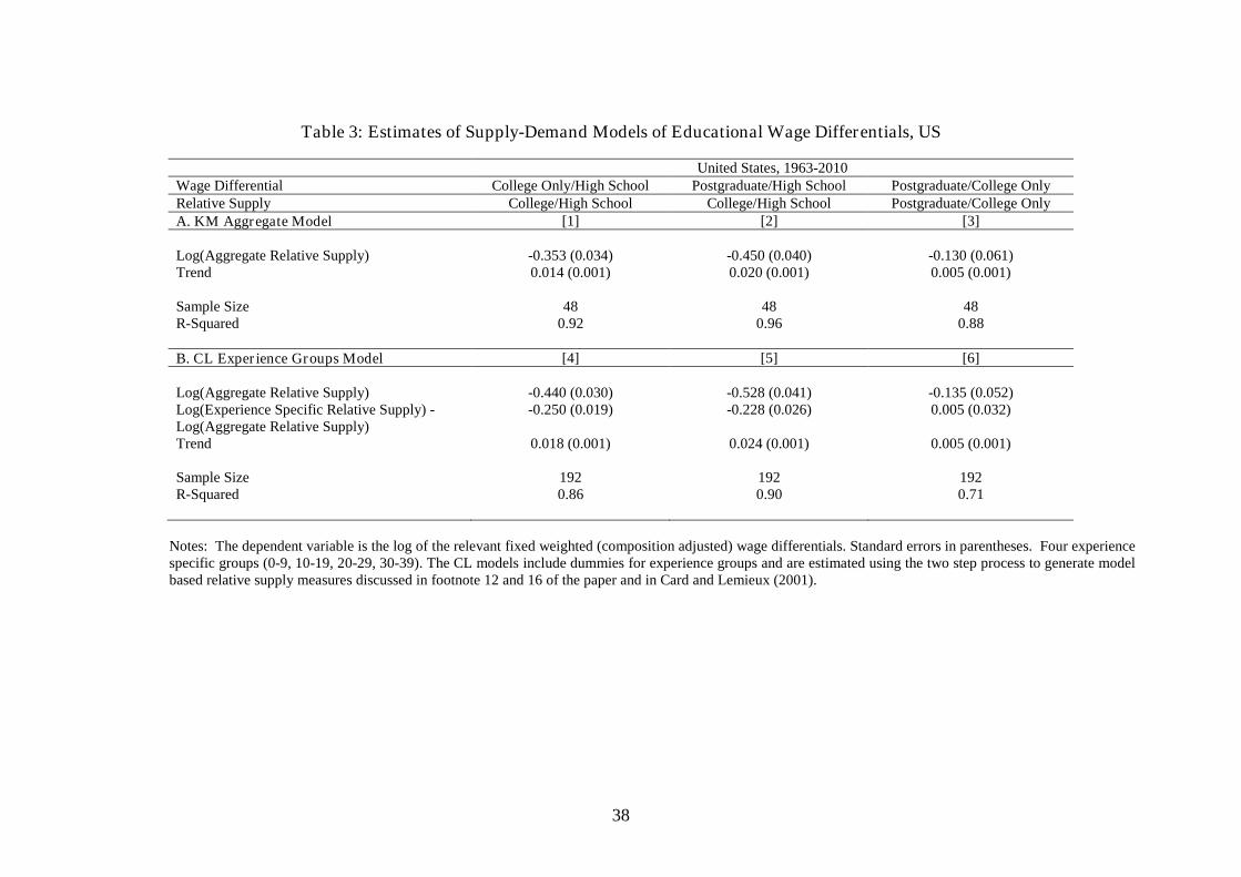
38

Table 3: Estimates of Supply-Demand Models of Educational Wage Differentials, US

United States, 1963-2010Wage Differential College Only/High School Postgraduate/High School Postgraduate/College OnlyRelative Supply College/High School College/High School Postgraduate/College OnlyA. KM Aggregate Model [1] [2] [3]

Log(Aggregate Relative Supply) -0.353 (0.034) -0.450 (0.040) -0.130 (0.061)Trend 0.014 (0.001) 0.020 (0.001) 0.005 (0.001)

Sample Size 48 48 48R-Squared 0.92 0.96 0.88

B. CL Experience Groups Model [4] [5] [6]

Log(Aggregate Relative Supply) -0.440 (0.030) -0.528 (0.041) -0.135 (0.052)Log(Experience Specific Relative Supply) -Log(Aggregate Relative Supply)

-0.250 (0.019) -0.228 (0.026) 0.005 (0.032)

Trend 0.018 (0.001) 0.024 (0.001) 0.005 (0.001)

Sample Size 192 192 192R-Squared 0.86 0.90 0.71

Notes: The dependent variable is the log of the relevant fixed weighted (composition adjusted) wage differentials. Standard errors in parentheses. Four experiencespecific groups (0-9, 10-19, 20-29, 30-39). The CL models include dummies for experience groups and are estimated using the two step process to generate modelbased relative supply measures discussed in footnote 12 and 16 of the paper and in Card and Lemieux (2001).

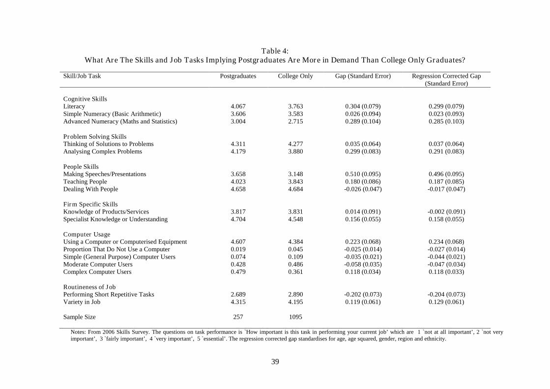
39

Table 4:What Are The Skills and Job Tasks Implying Postgraduates Are More in Demand Than College Only Graduates?

Skill/Job Task Postgraduates College Only Gap (Standard Error) Regression Corrected Gap(Standard Error)

Cognitive SkillsLiteracy 4.067 3.763 0.304 (0.079) 0.299 (0.079)Simple Numeracy (Basic Arithmetic) 3.606 3.583 0.026 (0.094) 0.023 (0.093)Advanced Numeracy (Maths and Statistics) 3.004 2.715 0.289 (0.104) 0.285 (0.103)

Problem Solving SkillsThinking of Solutions to Problems 4.311 4.277 0.035 (0.064) 0.037 (0.064)Analysing Complex Problems 4.179 3.880 0.299 (0.083) 0.291 (0.083)

People SkillsMaking Speeches/Presentations 3.658 3.148 0.510 (0.095) 0.496 (0.095)Teaching People 4.023 3.843 0.180 (0.086) 0.187 (0.085)Dealing With People 4.658 4.684 -0.026 (0.047) -0.017 (0.047)

Firm Specific SkillsKnowledge of Products/Services 3.817 3.831 0.014 (0.091) -0.002 (0.091)Specialist Knowledge or Understanding 4.704 4.548 0.156 (0.055) 0.158 (0.055)

Computer UsageUsing a Computer or Computerised Equipment 4.607 4.384 0.223 (0.068) 0.234 (0.068)Proportion That Do Not Use a Computer 0.019 0.045 -0.025 (0.014) -0.027 (0.014)Simple (General Purpose) Computer Users 0.074 0.109 -0.035 (0.021) -0.044 (0.021)Moderate Computer Users 0.428 0.486 -0.058 (0.035) -0.047 (0.034)Complex Computer Users 0.479 0.361 0.118 (0.034) 0.118 (0.033)

Routineness of JobPerforming Short Repetitive Tasks 2.689 2.890 -0.202 (0.073) -0.204 (0.073)Variety in Job 4.315 4.195 0.119 (0.061) 0.129 (0.061)

Sample Size 257 1095

Notes: From 2006 Skills Survey. The questions on task performance is `How important is this task in performing your current job’ which are 1 `not at all important’, 2 `not veryimportant’, 3 `fairly important’, 4 `very important’, 5 `essential’. The regression corrected gap standardises for age, age squared, gender, region and ethnicity.

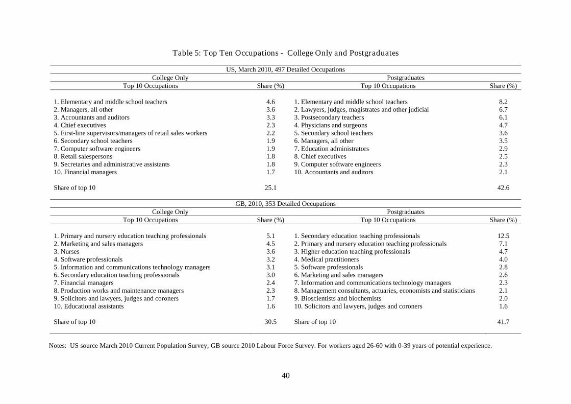
40

Table 5: Top Ten Occupations - College Only and Postgraduates

US, March 2010, 497 Detailed OccupationsCollege Only Postgraduates

Top 10 Occupations Share (%) Top 10 Occupations Share (%)

1. Elementary and middle school teachers 4.6 1. Elementary and middle school teachers 8.22. Managers, all other 3.6 2. Lawyers, judges, magistrates and other judicial 6.73. Accountants and auditors 3.3 3. Postsecondary teachers 6.14. Chief executives 2.3 4. Physicians and surgeons 4.75. First-line supervisors/managers of retail sales workers 2.2 5. Secondary school teachers 3.66. Secondary school teachers 1.9 6. Managers, all other 3.57. Computer software engineers 1.9 7. Education administrators 2.98. Retail salespersons 1.8 8. Chief executives 2.59. Secretaries and administrative assistants 1.8 9. Computer software engineers 2.310. Financial managers 1.7 10. Accountants and auditors 2.1

Share of top 10 25.1 42.6

GB, 2010, 353 Detailed OccupationsCollege Only Postgraduates

Top 10 Occupations Share (%) Top 10 Occupations Share (%)

1. Primary and nursery education teaching professionals 5.1 1. Secondary education teaching professionals 12.52. Marketing and sales managers 4.5 2. Primary and nursery education teaching professionals 7.13. Nurses 3.6 3. Higher education teaching professionals 4.74. Software professionals 3.2 4. Medical practitioners 4.05. Information and communications technology managers 3.1 5. Software professionals 2.86. Secondary education teaching professionals 3.0 6. Marketing and sales managers 2.67. Financial managers 2.4 7. Information and communications technology managers 2.38. Production works and maintenance managers 2.3 8. Management consultants, actuaries, economists and statisticians 2.19. Solicitors and lawyers, judges and coroners 1.7 9. Bioscientists and biochemists 2.010. Educational assistants 1.6 10. Solicitors and lawyers, judges and coroners 1.6

Share of top 10 30.5 Share of top 10 41.7

Notes: US source March 2010 Current Population Survey; GB source 2010 Labour Force Survey. For workers aged 26-60 with 0-39 years of potential experience.

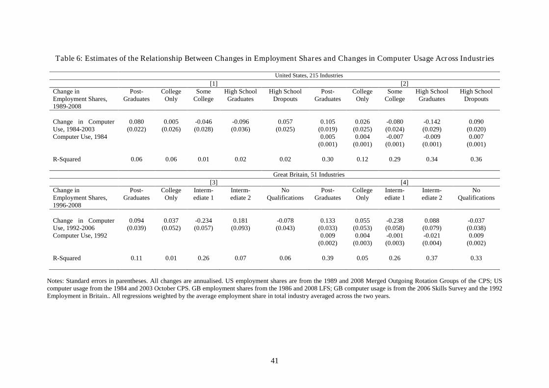
41

Table 6: Estimates of the Relationship Between Changes in Employment Shares and Changes in Computer Usage Across Industries

United States, 215 Industries

[1] [2]Change inEmployment Shares,1989-2008

Post-Graduates

CollegeOnly

SomeCollege

High SchoolGraduates

High SchoolDropouts

Post-Graduates

CollegeOnly

SomeCollege

High SchoolGraduates

High SchoolDropouts

Change in ComputerUse, 1984-2003

0.080(0.022)

0.005(0.026)

-0.046(0.028)

-0.096(0.036)

0.057(0.025)

0.105(0.019)

0.026(0.025)

-0.080(0.024)

-0.142(0.029)

0.090(0.020)

Computer Use, 1984 0.005(0.001)

0.004(0.001)

-0.007(0.001)

-0.009(0.001)

0.007(0.001)

R-Squared 0.06 0.06 0.01 0.02 0.02 0.30 0.12 0.29 0.34 0.36

Great Britain, 51 Industries[3] [4]

Change inEmployment Shares,1996-2008

Post-Graduates

CollegeOnly

Interm-ediate 1

Interm-ediate 2

NoQualifications

Post-Graduates

CollegeOnly

Interm-ediate 1

Interm-ediate 2

NoQualifications

Change in ComputerUse, 1992-2006

0.094(0.039)

0.037(0.052)

-0.234(0.057)

0.181(0.093)

-0.078(0.043)

0.133(0.033)

0.055(0.053)

-0.238(0.058)

0.088(0.079)

-0.037(0.038)

Computer Use, 1992 0.009(0.002)

0.004(0.003)

-0.001(0.003)

-0.021(0.004)

0.009(0.002)

R-Squared 0.11 0.01 0.26 0.07 0.06 0.39 0.05 0.26 0.37 0.33

Notes: Standard errors in parentheses. All changes are annualised. US employment shares are from the 1989 and 2008 Merged Outgoing Rotation Groups of the CPS; UScomputer usage from the 1984 and 2003 October CPS. GB employment shares from the 1986 and 2008 LFS; GB computer usage is from the 2006 Skills Survey and the 1992Employment in Britain.. All regressions weighted by the average employment share in total industry averaged across the two years.

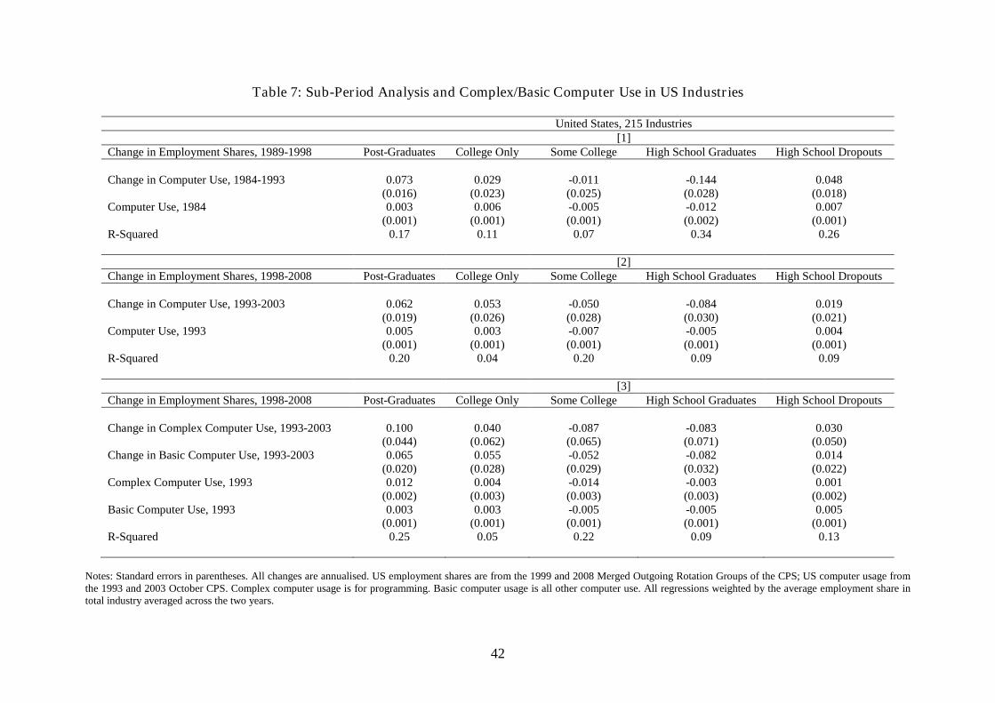
42

Table 7: Sub-Period Analysis and Complex/Basic Computer Use in US Industries

United States, 215 Industries[1]

Change in Employment Shares, 1989-1998 Post-Graduates College Only Some College High School Graduates High School Dropouts

Change in Computer Use, 1984-1993 0.073(0.016)

0.029(0.023)

-0.011(0.025)

-0.144(0.028)

0.048(0.018)

Computer Use, 1984 0.003(0.001)

0.006(0.001)

-0.005(0.001)

-0.012(0.002)

0.007(0.001)

R-Squared 0.17 0.11 0.07 0.34 0.26

[2]Change in Employment Shares, 1998-2008 Post-Graduates College Only Some College High School Graduates High School Dropouts

Change in Computer Use, 1993-2003 0.062(0.019)

0.053(0.026)

-0.050(0.028)

-0.084(0.030)

0.019(0.021)

Computer Use, 1993 0.005(0.001)

0.003(0.001)

-0.007(0.001)

-0.005(0.001)

0.004(0.001)

R-Squared 0.20 0.04 0.20 0.09 0.09

[3]Change in Employment Shares, 1998-2008 Post-Graduates College Only Some College High School Graduates High School Dropouts

Change in Complex Computer Use, 1993-2003 0.100(0.044)

0.040(0.062)

-0.087(0.065)

-0.083(0.071)

0.030(0.050)

Change in Basic Computer Use, 1993-2003 0.065(0.020)

0.055(0.028)

-0.052(0.029)

-0.082(0.032)

0.014(0.022)

Complex Computer Use, 1993 0.012(0.002)

0.004(0.003)

-0.014(0.003)

-0.003(0.003)

0.001(0.002)

Basic Computer Use, 1993 0.003(0.001)

0.003(0.001)

-0.005(0.001)

-0.005(0.001)

0.005(0.001)

R-Squared 0.25 0.05 0.22 0.09 0.13

Notes: Standard errors in parentheses. All changes are annualised. US employment shares are from the 1999 and 2008 Merged Outgoing Rotation Groups of the CPS; US computer usage fromthe 1993 and 2003 October CPS. Complex computer usage is for programming. Basic computer usage is all other computer use. All regressions weighted by the average employment share intotal industry averaged across the two years.

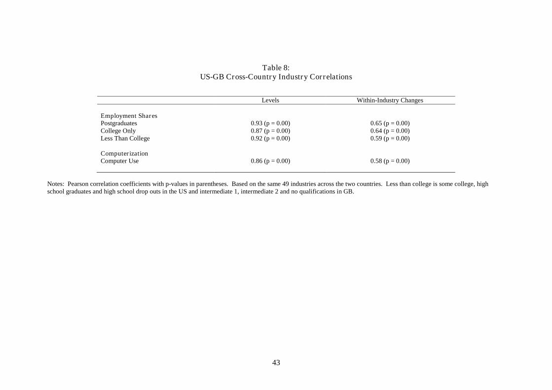
43

Table 8:US-GB Cross-Country Industry Correlations

Levels Within-Industry Changes

Employment SharesPostgraduates 0.93 (p = 0.00) 0.65 (p = 0.00)College Only 0.87 (p = 0.00) 0.64 (p = 0.00)Less Than College 0.92 (p = 0.00) 0.59 (p = 0.00)

ComputerizationComputer Use 0.86 (p = 0.00) 0.58 (p = 0.00)

Notes: Pearson correlation coefficients with p-values in parentheses. Based on the same 49 industries across the two countries. Less than college is some college, highschool graduates and high school drop outs in the US and intermediate 1, intermediate 2 and no qualifications in GB.

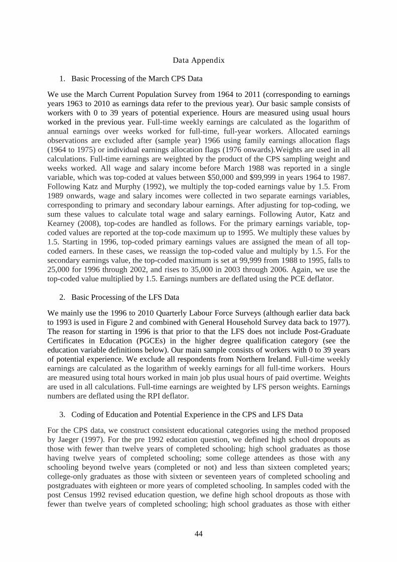
44

Data Appendix

1. Basic Processing of the March CPS Data

We use the March Current Population Survey from 1964 to 2011 (corresponding to earningsyears 1963 to 2010 as earnings data refer to the previous year). Our basic sample consists ofworkers with 0 to 39 years of potential experience. Hours are measured using usual hoursworked in the previous year. Full-time weekly earnings are calculated as the logarithm ofannual earnings over weeks worked for full-time, full-year workers. Allocated earningsobservations are excluded after (sample year) 1966 using family earnings allocation flags(1964 to 1975) or individual earnings allocation flags (1976 onwards).Weights are used in allcalculations. Full-time earnings are weighted by the product of the CPS sampling weight andweeks worked. All wage and salary income before March 1988 was reported in a singlevariable, which was top-coded at values between $50,000 and $99,999 in years 1964 to 1987.Following Katz and Murphy (1992), we multiply the top-coded earnings value by 1.5. From1989 onwards, wage and salary incomes were collected in two separate earnings variables,corresponding to primary and secondary labour earnings. After adjusting for top-coding, wesum these values to calculate total wage and salary earnings. Following Autor, Katz andKearney (2008), top-codes are handled as follows. For the primary earnings variable, top-coded values are reported at the top-code maximum up to 1995. We multiply these values by1.5. Starting in 1996, top-coded primary earnings values are assigned the mean of all top-coded earners. In these cases, we reassign the top-coded value and multiply by 1.5. For thesecondary earnings value, the top-coded maximum is set at 99,999 from 1988 to 1995, falls to25,000 for 1996 through 2002, and rises to 35,000 in 2003 through 2006. Again, we use thetop-coded value multiplied by 1.5. Earnings numbers are deflated using the PCE deflator.

2. Basic Processing of the LFS Data

We mainly use the 1996 to 2010 Quarterly Labour Force Surveys (although earlier data backto 1993 is used in Figure 2 and combined with General Household Survey data back to 1977).The reason for starting in 1996 is that prior to that the LFS does not include Post-GraduateCertificates in Education (PGCEs) in the higher degree qualification category (see theeducation variable definitions below). Our main sample consists of workers with 0 to 39 yearsof potential experience. We exclude all respondents from Northern Ireland. Full-time weeklyearnings are calculated as the logarithm of weekly earnings for all full-time workers. Hoursare measured using total hours worked in main job plus usual hours of paid overtime. Weightsare used in all calculations. Full-time earnings are weighted by LFS person weights. Earningsnumbers are deflated using the RPI deflator.

3. Coding of Education and Potential Experience in the CPS and LFS Data

For the CPS data, we construct consistent educational categories using the method proposedby Jaeger (1997). For the pre 1992 education question, we defined high school dropouts asthose with fewer than twelve years of completed schooling; high school graduates as thosehaving twelve years of completed schooling; some college attendees as those with anyschooling beyond twelve years (completed or not) and less than sixteen completed years;college-only graduates as those with sixteen or seventeen years of completed schooling andpostgraduates with eighteen or more years of completed schooling. In samples coded with thepost Census 1992 revised education question, we define high school dropouts as those withfewer than twelve years of completed schooling; high school graduates as those with either

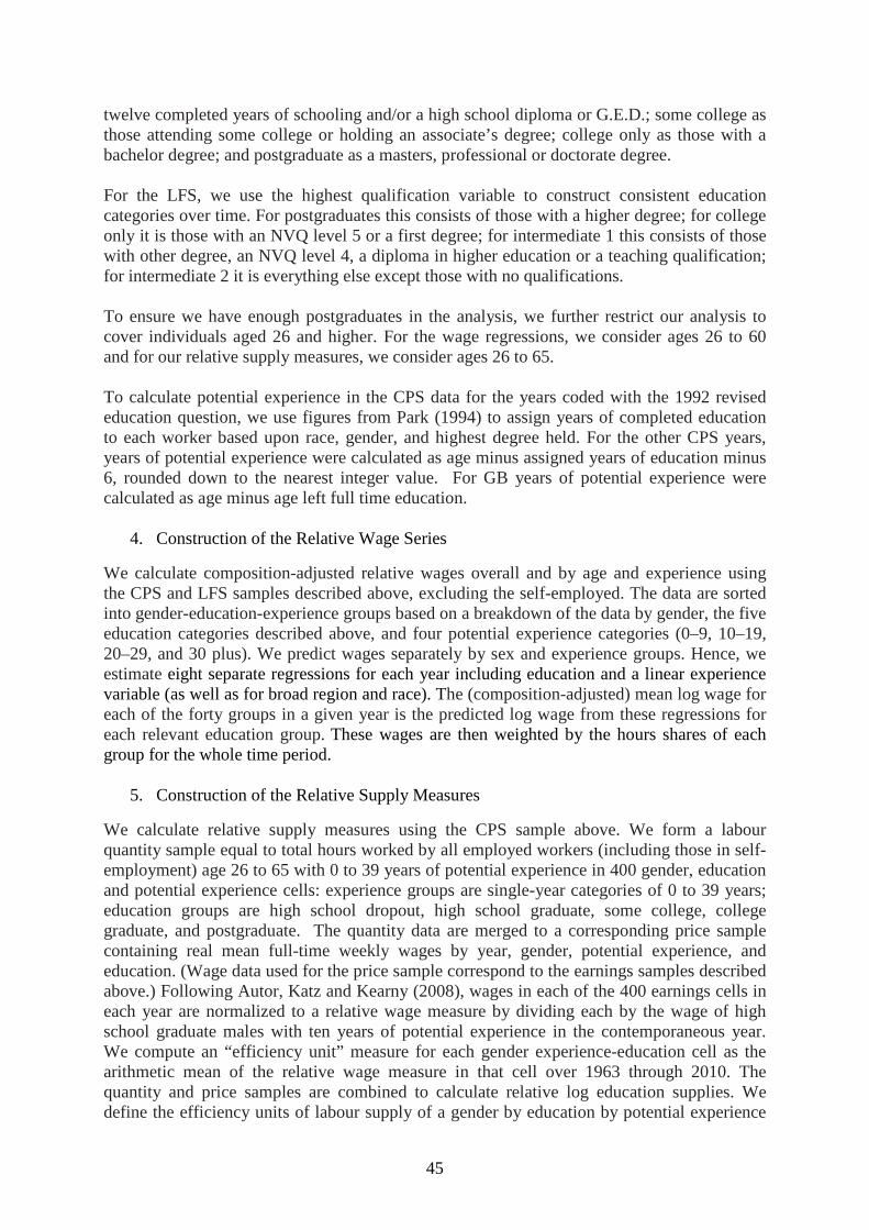
45

twelve completed years of schooling and/or a high school diploma or G.E.D.; some college asthose attending some college or holding an associate’s degree; college only as those with abachelor degree; and postgraduate as a masters, professional or doctorate degree.

For the LFS, we use the highest qualification variable to construct consistent educationcategories over time. For postgraduates this consists of those with a higher degree; for collegeonly it is those with an NVQ level 5 or a first degree; for intermediate 1 this consists of thosewith other degree, an NVQ level 4, a diploma in higher education or a teaching qualification;for intermediate 2 it is everything else except those with no qualifications.

To ensure we have enough postgraduates in the analysis, we further restrict our analysis tocover individuals aged 26 and higher. For the wage regressions, we consider ages 26 to 60and for our relative supply measures, we consider ages 26 to 65.

To calculate potential experience in the CPS data for the years coded with the 1992 revisededucation question, we use figures from Park (1994) to assign years of completed educationto each worker based upon race, gender, and highest degree held. For the other CPS years,years of potential experience were calculated as age minus assigned years of education minus6, rounded down to the nearest integer value. For GB years of potential experience werecalculated as age minus age left full time education.

4. Construction of the Relative Wage Series

We calculate composition-adjusted relative wages overall and by age and experience usingthe CPS and LFS samples described above, excluding the self-employed. The data are sortedinto gender-education-experience groups based on a breakdown of the data by gender, the fiveeducation categories described above, and four potential experience categories (0–9, 10–19,20–29, and 30 plus). We predict wages separately by sex and experience groups. Hence, weestimate eight separate regressions for each year including education and a linear experiencevariable (as well as for broad region and race). The (composition-adjusted) mean log wage foreach of the forty groups in a given year is the predicted log wage from these regressions foreach relevant education group. These wages are then weighted by the hours shares of eachgroup for the whole time period.

5. Construction of the Relative Supply Measures

We calculate relative supply measures using the CPS sample above. We form a labourquantity sample equal to total hours worked by all employed workers (including those in self-employment) age 26 to 65 with 0 to 39 years of potential experience in 400 gender, educationand potential experience cells: experience groups are single-year categories of 0 to 39 years;education groups are high school dropout, high school graduate, some college, collegegraduate, and postgraduate. The quantity data are merged to a corresponding price samplecontaining real mean full-time weekly wages by year, gender, potential experience, andeducation. (Wage data used for the price sample correspond to the earnings samples describedabove.) Following Autor, Katz and Kearny (2008), wages in each of the 400 earnings cells ineach year are normalized to a relative wage measure by dividing each by the wage of highschool graduate males with ten years of potential experience in the contemporaneous year.We compute an “efficiency unit” measure for each gender experience-education cell as thearithmetic mean of the relative wage measure in that cell over 1963 through 2010. Thequantity and price samples are combined to calculate relative log education supplies. Wedefine the efficiency units of labour supply of a gender by education by potential experience

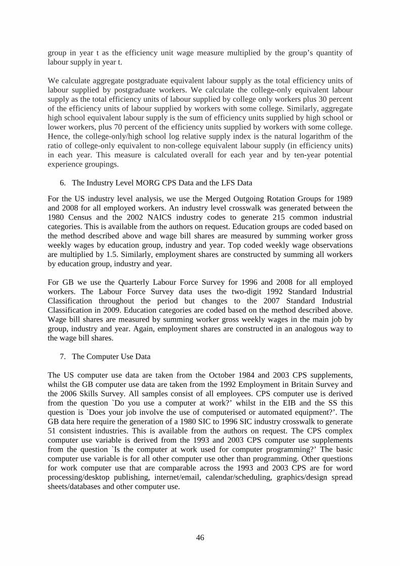
46

group in year t as the efficiency unit wage measure multiplied by the group’s quantity oflabour supply in year t.

We calculate aggregate postgraduate equivalent labour supply as the total efficiency units oflabour supplied by postgraduate workers. We calculate the college-only equivalent laboursupply as the total efficiency units of labour supplied by college only workers plus 30 percentof the efficiency units of labour supplied by workers with some college. Similarly, aggregatehigh school equivalent labour supply is the sum of efficiency units supplied by high school orlower workers, plus 70 percent of the efficiency units supplied by workers with some college.Hence, the college-only/high school log relative supply index is the natural logarithm of theratio of college-only equivalent to non-college equivalent labour supply (in efficiency units)in each year. This measure is calculated overall for each year and by ten-year potentialexperience groupings.

6. The Industry Level MORG CPS Data and the LFS Data

For the US industry level analysis, we use the Merged Outgoing Rotation Groups for 1989and 2008 for all employed workers. An industry level crosswalk was generated between the1980 Census and the 2002 NAICS industry codes to generate 215 common industrialcategories. This is available from the authors on request. Education groups are coded based onthe method described above and wage bill shares are measured by summing worker grossweekly wages by education group, industry and year. Top coded weekly wage observationsare multiplied by 1.5. Similarly, employment shares are constructed by summing all workersby education group, industry and year.

For GB we use the Quarterly Labour Force Survey for 1996 and 2008 for all employedworkers. The Labour Force Survey data uses the two-digit 1992 Standard IndustrialClassification throughout the period but changes to the 2007 Standard IndustrialClassification in 2009. Education categories are coded based on the method described above.Wage bill shares are measured by summing worker gross weekly wages in the main job bygroup, industry and year. Again, employment shares are constructed in an analogous way tothe wage bill shares.

7. The Computer Use Data

The US computer use data are taken from the October 1984 and 2003 CPS supplements,whilst the GB computer use data are taken from the 1992 Employment in Britain Survey andthe 2006 Skills Survey. All samples consist of all employees. CPS computer use is derivedfrom the question `Do you use a computer at work?’ whilst in the EIB and the SS thisquestion is `Does your job involve the use of computerised or automated equipment?’. TheGB data here require the generation of a 1980 SIC to 1996 SIC industry crosswalk to generate51 consistent industries. This is available from the authors on request. The CPS complexcomputer use variable is derived from the 1993 and 2003 CPS computer use supplementsfrom the question `Is the computer at work used for computer programming?’ The basiccomputer use variable is for all other computer use other than programming. Other questionsfor work computer use that are comparable across the 1993 and 2003 CPS are for wordprocessing/desktop publishing, internet/email, calendar/scheduling, graphics/design spreadsheets/databases and other computer use.

47

8. The Skills Survey Job Tasks Data

The 2006 Skills Survey contains questions on task performance and educational qualificationsfor over 2,467 working men and women. Respondents are asked the question `How importantis this task in performing your current job’ which are 1 `not at all important’, 2 `not veryimportant’, 3 `fairly important’, 4 `very important’, 5 `essential’. We define postgraduateworkers as having a Masters or PhD and college only workers as having a university orCNAA degree.

9. Data for the Polarization Analysis

In this part of the analysis we used data from the 5% PUMS 1980 Decennial Census data, aswell as the 1 % samples from the 2009, 2010 and 2011 American Community Surveys (werefer to the pooled 2009-2011 sample as 2010). The basic sample consists of all workingindividuals aged 18-65. Hours are measured using usual hours worked in the previous year.We construct consistent educational categories in the 1980 and 2010 data as described in 3.above. The skill percentiles are based upon 320 consistently defined occupations for all thosein employment (hours > 0). The procedures followed in Autor and Dorn (2013) and Lefterand Sand (2011) were used to obtain the consistent definitions. The 320 occupations aredivided into employment weighted percentiles and deciles based upon the mean occupationalwage in 1980.