The Robustness of Rasch True Score Preequating to

University of South FloridaScholar Commons

Graduate Theses and Dissertations Graduate School

10-22-2008

The Robustness of Rasch True Score Preequatingto Violations of Model Assumptions UnderEquivalent and Nonequivalent PopulationsGarron GianopulosUniversity of South Florida

Follow this and additional works at: https://scholarcommons.usf.edu/etd

Part of the American Studies Commons

This Dissertation is brought to you for free and open access by the Graduate School at Scholar Commons. It has been accepted for inclusion inGraduate Theses and Dissertations by an authorized administrator of Scholar Commons. For more information, please [email protected].

Scholar Commons CitationGianopulos, Garron, "The Robustness of Rasch True Score Preequating to Violations of Model Assumptions Under Equivalent andNonequivalent Populations" (2008). Graduate Theses and Dissertations.https://scholarcommons.usf.edu/etd/259

http://scholarcommons.usf.edu/?utm_source=scholarcommons.usf.edu%2Fetd%2F259&utm_medium=PDF&utm_campaign=PDFCoverPages

http://scholarcommons.usf.edu/?utm_source=scholarcommons.usf.edu%2Fetd%2F259&utm_medium=PDF&utm_campaign=PDFCoverPages

https://scholarcommons.usf.edu?utm_source=scholarcommons.usf.edu%2Fetd%2F259&utm_medium=PDF&utm_campaign=PDFCoverPages

https://scholarcommons.usf.edu/etd?utm_source=scholarcommons.usf.edu%2Fetd%2F259&utm_medium=PDF&utm_campaign=PDFCoverPages

https://scholarcommons.usf.edu/grad?utm_source=scholarcommons.usf.edu%2Fetd%2F259&utm_medium=PDF&utm_campaign=PDFCoverPages

https://scholarcommons.usf.edu/etd?utm_source=scholarcommons.usf.edu%2Fetd%2F259&utm_medium=PDF&utm_campaign=PDFCoverPages

http://network.bepress.com/hgg/discipline/439?utm_source=scholarcommons.usf.edu%2Fetd%2F259&utm_medium=PDF&utm_campaign=PDFCoverPages

mailto:[email protected]

The Robustness of Rasch True Score Preequating to Violations of Model Assumptions

Under Equivalent and Nonequivalent Populations

by

Garron Gianopulos

A dissertation submitted in partial fulfillment of the requirements for the degree of

Doctor of Philosophy Department of Educational Measurement and Research

College of Education University of South Florida

Major Professor: John Ferron, Ph.D. Robert Dedrick, Ph.D. Yi-Hsin Chen, Ph.D. Stephen Stark, Ph.D.

Date of Approval: October 22, 2008

Keywords: Item Response Theory, Equating to a Calibrated Item Bank, Multidimensionality, Fixed Parameter Calibration, Stocking and Lord Linking

©Copyright 2008, Garron Gianopulos

DEDICATION

I dedicate this dissertation to my parents and to my wife. I dedicate this work to

my parents for their loving support and encouragement. They gave me a wonderful

upbringing, a stable home, and an enduring faith. I have been very fortunate indeed to

have been raised and cared for by such fine people. My parents instilled in me an

appreciation and respect for truth and a love for learning. For this, I am deeply grateful.

I also dedicate this dissertation to my wife. For me, this dissertation represents

the culmination of six years of course work and thousands of hours of labor conducting

the dissertation study; for my wife, this dissertation represents countless personal

sacrifices on my behalf. Completing a doctoral degree certainly requires much from the

spouse of a student. Our situation was no exception. The demands of full time

employment and course work at times left little of me to give to my wife and daughter;

nonetheless, my wife fulfilled her roles of wife, mother, and, most recently, employee

without complaint. She has remained steadfastly supportive, both in words and in deeds,

through my entire graduate education experience. Clearly this dissertation is an

accomplishment I share with my family, without which I would neither have had the

inspiration to start, nor the wherewithal to complete.

ACKNOWLEDGEMENTS

I want to thank all members of the doctoral committee for their time, their energy,

and their thoughtful input to all phases of the research process. Each member of the

committee contributed in unique ways to this study. Dr. Chen provided many practical

suggestions that improved the structure of my proposal document, the clarity of my

research questions, and the completeness of the results. Dr. Dedrick’s course in research

design and his editorial comments helped me improve the design, readability, and internal

consistency of the document. Dr. Dedrick lent me, and eventually gave me, his personal

copy of Kolen and Brennan’s Test Equating, Scaling, and Linking: Methods and

Practices, which proved to be an invaluable resource for this study. Dr. Stark

encouraged me to conduct research in IRT through coursework, lectures, publications,

and many one-on-one conversations. Dr. Stark’s suggestion to include item parameter

error as an outcome measure and relate it to equating error, proved to be very useful in

explaining my results. I especially want to thank Dr. Ferron for his assistance in

planning, conducting, and writing the study. His guidance through technical difficulties

and all phases of the dissertation process was invaluable. Dr. Ferron was always

available, attentive to my questions, and full of suggestions.

i

TABLE OF CONTENTS

LIST OF TABLES ...............................................................................................................v

LIST OF FIGURES ........................................................................................................... vi

CHAPTER ONE: INTRODUCTION ..................................................................................1

Organization of the Paper .................................................................................................2

Preview of Chapter One ...................................................................................................3

Rationale for Equating .....................................................................................................3

Scores Used in Equating ..................................................................................................6

Rationale for True Score Preequating to a Calibrated Item Pool ...................................10

Statement of the Problem ...............................................................................................12

Purpose of the Study ......................................................................................................16

Research Questions ........................................................................................................17

Importance of the Study .................................................................................................18

Definition of Terms ........................................................................................................20

CHAPTER TWO: LITERATURE REVIEW ....................................................................26

Equating in the Context of Linking ................................................................................26

Prediction ....................................................................................................................27

Scale Alignment .........................................................................................................28

Test Equating ..............................................................................................................29

Data Collection Designs for Equating ............................................................................32

Random Groups Design..............................................................................................32

ii

Single Groups with Counterbalancing Design ...........................................................33

Common Item Designs ...............................................................................................33

Equating Methods ..........................................................................................................34

Identity Equating ........................................................................................................35

Linear Equating ..........................................................................................................36

Introduction to IRT Equating .....................................................................................40

IRT Equating Methods ...............................................................................................42

Factors Affecting IRT Equating Outcomes ....................................................................53

Assumption of Unidimensionality ..............................................................................54

Assumption of Equal Discriminations ........................................................................56

Assumption of Minimal Guessing ..............................................................................57

Quality of Common Items ..........................................................................................59

Equivalence of Populations ........................................................................................61

Method of Calibration ................................................................................................64

Summary of Literature Review ......................................................................................66

The Need for More Research on Preequating with the Rasch Model ............................68

CHAPTER THREE: METHODS ......................................................................................70

Purpose of the Study ......................................................................................................70

Research Questions ........................................................................................................70

Hypotheses .....................................................................................................................72

Study Design ..................................................................................................................73

Factors Held Constant in Phase One ..........................................................................73

Manipulated Factors in Phase One .............................................................................74

Equating Criteria.........................................................................................................78

iii

Parameter Recovery ....................................................................................................80

Phase One Conditions .................................................................................................80

Simulation Methods .......................................................................................................82

Data .............................................................................................................................82

Item Linking Simulation Procedures ..........................................................................83

Phase Two ......................................................................................................................85

Phase Two Manipulated Factors.................................................................................86

Phase Two Conditions ................................................................................................86

Phase Two Simulation Procedures .................................................................................89

CHAPTER FOUR: RESULTS ..........................................................................................92

Research Question 1 ...................................................................................................94



Research Question 4 .................................................................................................100

Phase Two ....................................................................................................................101

Research Question 5a ...............................................................................................102

Research Question 5b ...............................................................................................108

Research Question 5c ...............................................................................................108

Research Question 5d ...............................................................................................109

CHAPTER FIVE: DISCUSSION ....................................................................................115

Phase One .................................................................................................................115

Phase Two.................................................................................................................117

Hypotheses................................................................................................................118

Recommendations ....................................................................................................127

iv

Limitations ................................................................................................................130

Future research .........................................................................................................132

Conclusion ................................................................................................................134

APPENDIX A: SAS CODE............................................................................................147

APPENDIX B: DESCRIPTIVE STATISTICS OF GENERATED TEST FORMS ......242

APPENDIX C: DESCRIPTIVE STATISTICS FOR GENERATED THETA DISTRIBUTIONS ................................................................................248

ABOUT THE AUTHOR ....................................................................................... End Page

v

LIST OF TABLES

Table 1. Form to Form Equating Versus Preequating to a Calibrated Item Pool .............11

Table 2. A Plan to Create a Calibrated Item Pool .............................................................53

Table 3. Design Matrix for Main Effects ..........................................................................81

Table 4. Design Matrix for Phase Two .............................................................................88

Table 5. Steps to Calculating Bootstrap Standard Error and Bias Across Specified Number of Forms ................................................................................................91

Table 6. Mean Absolute Bias of Equating by Method ....................................................103

Table 7. Variance of Equating Bias ................................................................................104

Table 8. Mean Standard Error of Equating (MSEE) by Method ....................................106

Table 9. Variance of the Standard Error of Equating by Method ...................................107

Table 10. Mean Absolute Bias Across All Conditions ...................................................110

vi

LIST OF FIGURES Figure 1. Steps to IRT Equating .......................................................................................43

Figure 2. Steps to IRT Preequating ...................................................................................51

Figure 3. Generated Theta Distributions at Five Levels of Population Nonequivalence................................................................................................82

Figure 4. Bootstrap Standard Errors of Equating for 20 and 50 replications. ..................82

Figure 5. Linking Plan and Assignment of Items to Forms in Phase One ........................85

Figure 6. Linking Plan and Assignment of Items to Forms in Phase Two .......................90

Figure 7. Ideal Conditions and Equating Outcomes.. .......................................................93

Figure 8. Equating Outcomes Under the Severely Violated Assumption of Unidimensionality. ...........................................................................................95

Figure 9. Equating Outcomes Under Severely Nonequivalent Populations. ....................97

Figure 10. Equating Outcomes Under Severely Nonequivalent Item Discriminations. ...............................................................................................99

Figure 11. Equating Outcomes Under Severe Guessing.. ...............................................101

Figure 12. The Mean Standard Error of Equating and the Mean Bias of Equating of All Conditions by Method. ........................................................................109

Figure 13. Standard Errors of Equating and Bias Across Five Forms under Ideal Conditions. .....................................................................................................111

Figure 14. Standard Errors of Equating and Bias Across Five Forms under Moderately Violated Assumptions. ...............................................................112

Figure 15. Standard Errors of Equating and Bias Across Five Forms under Severely Violated Model Assumptions. ........................................................113

vii

Figure 16. Standard Errors of equating and Bias Across Five Forms under the Most Severely Violated Model Assumptions.. ..............................................114

Figure 17. Equating Outcomes under the Interaction of Moderate Guessing and Moderate Nonequivalent Item Discriminations. ............................................120

Figure 18. Equating Outcomes under the Interaction of Severe Guessing and Moderate Levels of Nonequivalent Item Discriminations. ............................122

Figure 19. Equating Outcomes When All Assumptions are Satisfied and the Difficulty of the Test is Misaligned with the Ability of the Examinees. .......125

viii

THE ROBUSTNESS OF RASCH TRUE SCORE PREEQUATING TO VIOLATIONS

OF MODEL ASSUMPTIONS UNDER EQUIVALENT AND NONEQUIVALENT POPULATIONS

Garron Gianopulos

ABSTRACT

This study examined the feasibility of using Rasch true score preequating under

violated model assumptions and nonequivalent populations. Dichotomous item responses

were simulated using a compensatory two dimensional (2D) three parameter logistic

(3PL) Item Response Theory (IRT) model. The Rasch model was used to calibrate

difficulty parameters using two methods: Fixed Parameter Calibration (FPC) and separate

calibration with the Stocking and Lord linking (SCSL) method. A criterion equating

function was defined by equating true scores calculated with the generated 2D 3PL IRT

item and ability parameters, using random groups equipercentile equating. True score

preequating to FPC and SCSL calibrated item banks was compared to identity and

Levine’s linear true score equating, in terms of equating bias and bootstrap standard

errors of equating (SEE) (Kolen & Brennan, 2004). Results showed preequating was

robust to simulated 2D 3PL data and to nonequivalent item discriminations, however,

true score equating was not robust to guessing and to the interaction of guessing and

nonequivalent item discriminations. Equating bias due to guessing was most marked at

the low end of the score scale. Equating an easier new form to a more difficult base form

produced negative bias. Nonequivalent item discriminations interacted with guessing to

ix

magnify the bias and to extend the range of the bias toward the middle of the score

distribution. Very easy forms relative to the ability of the examinees also produced

substantial error at the low end of the score scale. Accumulating item parameter error in

the item bank increased the SEE across five forms. Rasch true score preequating

produced less equating error than Levine’s true score linear equating in all simulated

conditions. FPC with Bigsteps performed as well as separate calibration with the

Stocking and Lord linking method. These results support earlier findings, suggesting that

Rasch true score preequating can be used in the presence of guessing if accuracy is

required near the mean of the score distribution, but not if accuracy is required with very

low or high scores.

1

CHAPTER ONE

INTRODUCTION

Equating is an important component of any testing program that produces more

than one form for a test. Equating places scores from different forms onto a single scale.

Once scores are on a single scale, scores from different forms are interchangeable

(Holland & Dorans, 2006; Kolen & Brennan, 2004). This permits standards defined on

one test form to be applied to other forms, permitting classification decisions to be

consistent and accurate across forms. Without equating, scores from different forms

would not be interchangeable, scores would not be comparable, and classification

decisions made across forms would not be consistent or accurate. For this reason,

equating is critically important to testing programs that use test scores for the

measurement of growth and for classifying examinees into categories. When equating is

properly performed, scores and the decisions made from them can be consistent, accurate,

and fair.

This study compares one type of equating, preequating, to conventional equating

designs in terms of random and systematic equating error. Preequating differs from

conventional equating in that preequating uses predicted scores rather than observed

scores for equating purposes. Preequating is especially useful for testing programs that

need to report scores immediately at the conclusion of a test. Preequating has a research

history of mixed results. The purpose of this study is to determine the limitations of

2

preequating under testing conditions that past researchers have found to affect

preequating.

Organization of the Paper

Chapter one is an introduction to the topic of equating and the purpose of the

study. An explanation of the research problem, a rationale for the research focus, and the

research questions are provided. Chapter Two presents a literature review of relevant

research, and, as a whole, provides support for the research questions. Chapter Three

presents the chosen research design, measures, manipulated factors, simulation design,

and data analysis. Chapter four presents the results of the simulation study. Chapter five

presents a discussion of the results and provides recommendations to practitioners.

The research questions that are being addressed by this study are relevant to a

wide range of professionals that span the spectrum of test developers, psychometricians,

and researchers in education, certification, and licensing fields. The audience for this

study includes anyone who wants to know the practical limitations of preequating. This

study is particularly relevant to those who use dichotomously scored tests and who desire

to preequate on the basis of small sample sizes of 100 to 500 examinees per test form.

Psychometricians who need additional guidance in evaluating the appropriateness of

preequating to a calibrated item pool for their particular testing program should find this

study informative. This paper has been written for a professional and academic audience

that has minimal exposure to test equating.

3

Preview of Chapter One

Given the technical nature of the research questions of this study, I devote the

introductory chapter to presenting the conceptual background of the study. First, I

provide an overview of equating, including the rationale of equating and preequating. I

then discuss scores that are used in equating, including true scores, equated scores, and

scale scores. After providing an explanation of scores used in equating, I present the

rationale, purpose, and questions of the research study. A list of psychometric terms used

throughout this paper is provided at the end of Chapter One.

Rationale for Equating

When test forms are used with high stakes tests, cheating is a continual threat to

the validity of the test scores. Cheating has many undesirable consequences including a

reduction of test reliability, test validity, and an increase in false positive classifications

in criterion referenced tests (Cizek, 2001). In an effort to combat cheating and the

learning of items, testing programs track, limit, and balance the exposure of items.

Testing programs often strive to create large item banks to support the production of

multiple alternate forms, so that new items are continually being introduced to the would-

be cheater. Alternate forms are forms that have equivalent content and are administered

in a standardized manner, but are not necessarily equivalent statistically (AERA, APA, &

NCME, 1999).

Even though efforts are made to make alternate test forms as similar as possible,

4

small differences in form difficulty appear across forms. When the groups taking two

forms are equivalent in ability, form differences manifest as differences in number

correct (NC) raw scores. Number correct scores are calculated by summing the scored

responses. If the differences in form difficulty are ignored, the NC raw score of

individual examinees to some degree depends on the particular form they received.

Easier forms increase NC raw scores, while more difficult forms lower NC raw scores of

an equivalent group. In tests that produce pass/fail decisions, these small changes in form

difficulty increase classification error. Therefore, the percentage of examinees passing a

test to some degree depends on the particular form taken. Easier forms increase the

percent passing, while more difficult forms lower the percent passing of equivalent

groups. In real testing situations, groups of examinees are usually not equivalent unless

care is taken to control for differences in ability between groups. Without controlling test

form equivalence and population equivalence, group ability differences and test form

difficulty differences become confounded (Kolen & Brennan, 2004). Resulting NC raw

scores depend on the interaction of ability and test form difficulty, rather than solely on

the ability of an examinee.

To prevent the confounding of group ability and test form difficulty,

psychometricians have developed a large number of data collection designs. An

equating data collection design is the process by which test data are collected for

equating, in such a way that ability differences between groups taking forms can be

controlled. Some designs, such as the random groups design, control ability differences

through random assignment of forms to examinees. The random groups design can be

considered an example of an equivalent groups design (Von Davier, Holland, & Thayer,

5

2004), because the method produces groups of equivalent ability, thereby disconfounding

ability differences from form differences in NC raw scores. Other data collection designs

control for ability differences across forms through statistical procedures. For instance,

in linear equating under the common item nonequivalent groups design (CINEG),

examined in this study, common items are used across forms to estimate the abilities of

the two groups, allowing ability and form differences to be disconfounded. Additional

equating data collection designs are presented in Chapter Two.

While there are few equating designs, there are many equating methods. An

equating method is a mathematical procedure that places NC raw scores from one

alternate form onto the scale of another form, such that the scores across forms are

interchangeable. Equating methods are based on Classical True Score Theory (CTT) or

Item Response Theory (IRT). With the exception of identity equating, which assumes

scores from two forms are already on the same scale, equating methods work by aligning

the relative position of scores within the distribution across forms using a select statistic.

For instance, in equivalent groups mean equating, it is assumed that the mean NC score

on a new form is equivalent to the mean NC score on the base form. The equating

relationship between the mean NC scores is applied to all scores (Kolen & Brennan,

2004). In equivalent groups linear equating, z scores are used as the basis of aligning

scores (Crocker & Algina, 1986). Z scores are obtained by subtracting each NC raw

score from the mean raw score and dividing by the standard deviation. In linear equating,

a z score of 1 is assumed to be equivalent to a z score of 1 on the base form. Linear

equating assumes that a linear formula can explain the equating relationship, hence, the

magnitude of the score adjustments vary across the score continuum. In equivalent

6

groups equipercentile equating, percentiles are used to align scores (Crocker & Algina,

1986). Under this equating method, the new form score associated with the 80th

percentile, for example, is considered to be equivalent to the score associated with the

80th percentile on the base form. Equipercentile equating produces a curvilinear function.

In IRT true score equating, estimates of the latent ability, theta, are used to align scores.

In IRT true score equating, a NC raw score associated with a theta estimate of 2.2 on the

new form is assumed to be equivalent to a NC raw score associated with a theta estimate

of 2.2 on the base form. Like equipercentile equating, IRT equating produces a

curvilinear function.

Scores Used in Equating

The most commonly used score for equating is the NC raw score (Crocker &

Algina, 1986; Kolen & Brennan, 2004). NC raw scores are often preferred over formula

scores because of their simplicity. Examinees have little trouble understanding the

meaning of raw scores. Even in many IRT applications that produce estimates of the

latent ability distribution theta, NC raw scores are often used rather than thetas. An

equating process places NC raw scores of a new form onto the scale of the base form.

These equated scores are referred to as equivalent raw scores. An equivalent raw score

for a new form is the expected NC raw score of a given examinee on the base form.

Equivalent raw scores are continuous measures, and can be rounded to produce rounded

equivalent raw scores. Rounded equivalent raw scores can be used for reporting

purposes; however, Kolen and Brennan report that examinees tend to confuse rounded

7

equivalent raw scores with NC raw scores (2004).

To prevent the confusion of rounded equivalent raw scores with NC raw scores,

testing organizations prefer to use a primary scale. A primary scale is designed expressly

for reporting scores to examinees. Equivalent raw scores from any number of forms can

be placed on the primary scale. The end result is scale scores that are completely

interchangeable, regardless of what form the score originated from. Just like rounded

equivalent scores, scale scores permit examinee scores to be compared regardless of what

form the scores originated from; however, there is less risk that examinees will confuse

the NC raw score with the scale score. Another benefit to using a primary scale score

rather than a rounded equivalent raw score, is that fact that normative information and

content information can be integrated into a primary scale (Kolen & Brennan, 2004).

NC raw scores are not the only type of scores that can be used for equating. In

true score equating, true scores of examinees are equated rather than NC scores. The true

score equating relationship is then applied to NC raw scores. The definition of a true

score depends on the test theory used. According to CTT, a true score is defined as the

hypothetical mean score of an infinite number of parallel tests administered to an

examinee (Crocker & Algina, 1986). In CTT, true scores are equivalent to NC raw

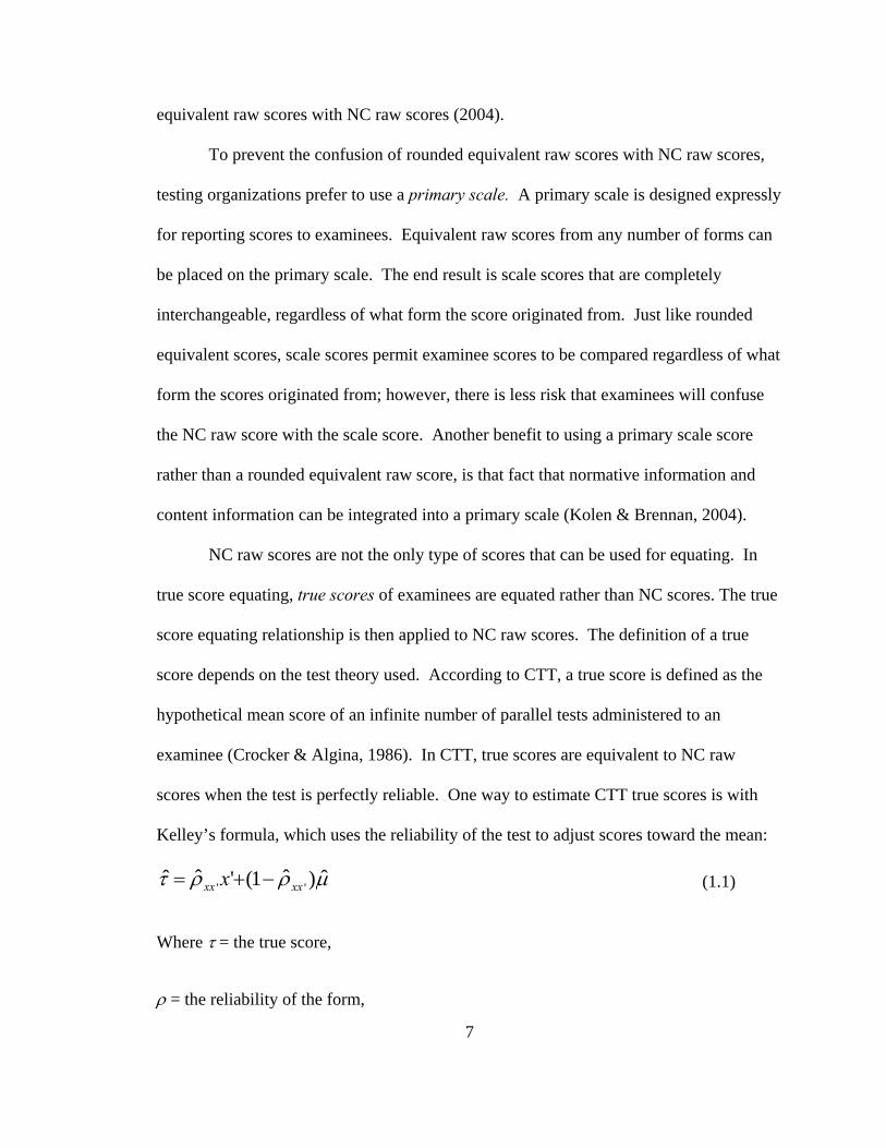
scores when the test is perfectly reliable. One way to estimate CTT true scores is with

Kelley’s formula, which uses the reliability of the test to adjust scores toward the mean:

μρρτ ˆ)ˆ1('ˆˆ '' xxxx x −+= (1.1)

Where τ = the true score,

ρ = the reliability of the form,

8

μ = the mean of the NC raw score, and

x = observed scores.

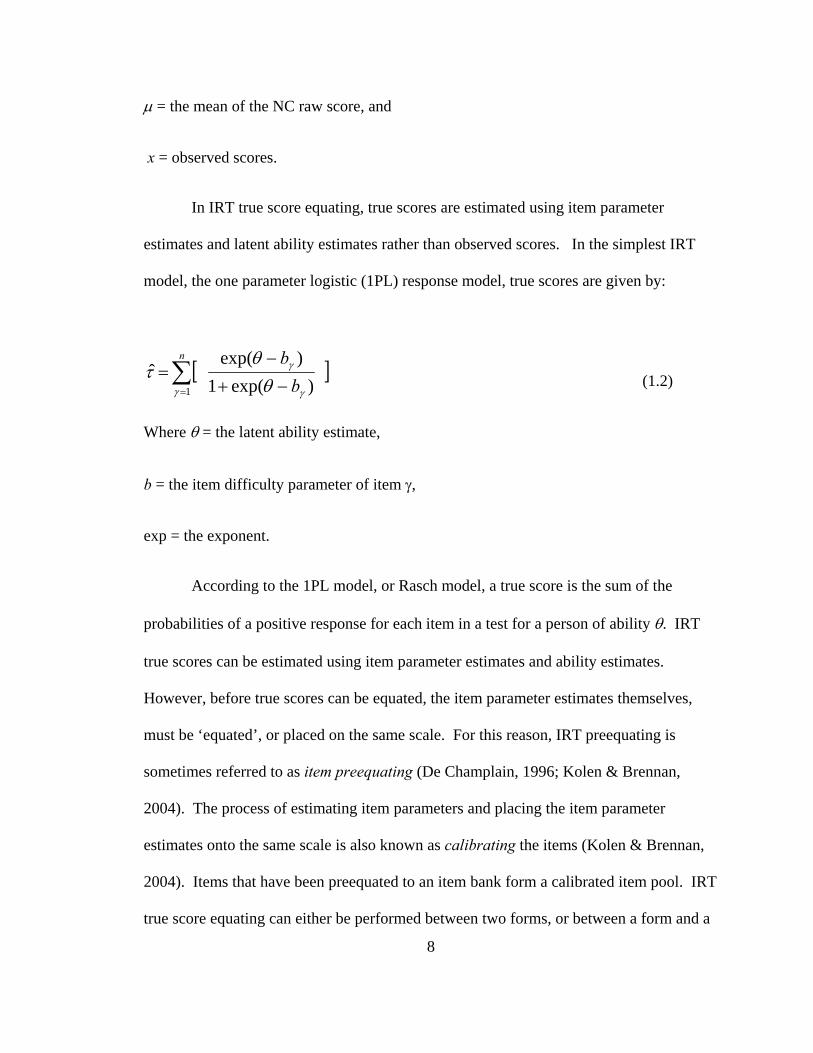
In IRT true score equating, true scores are estimated using item parameter

estimates and latent ability estimates rather than observed scores. In the simplest IRT

model, the one parameter logistic (1PL) response model, true scores are given by:

(1.2)

Where θ = the latent ability estimate,

b = the item difficulty parameter of item γ,

exp = the exponent.

According to the 1PL model, or Rasch model, a true score is the sum of the

probabilities of a positive response for each item in a test for a person of ability θ. IRT

true scores can be estimated using item parameter estimates and ability estimates.

However, before true scores can be equated, the item parameter estimates themselves,

must be ‘equated’, or placed on the same scale. For this reason, IRT preequating is

sometimes referred to as item preequating (De Champlain, 1996; Kolen & Brennan,

2004). The process of estimating item parameters and placing the item parameter

estimates onto the same scale is also known as calibrating the items (Kolen & Brennan,

2004). Items that have been preequated to an item bank form a calibrated item pool. IRT

true score equating can either be performed between two forms, or between a form and a

[ ]∑= − +

− =

n

bb

1 )exp(1)exp(

ˆγ γ

γ

θθ

τ

9

calibrated item pool. Because the probability of a positive response can be estimated for

each item, items can be selected for a new form and the expected test score can be

estimated in the form of a true score, even though the entire form has not been

administered.

While IRT does provide many benefits, including greater precision in

measurement and greater flexibility in test assembly, the validity of the model rests on

the satisfaction of model assumptions. Violations of these assumptions may render IRT

equating less effective than CTT equating. For this reason, this study simulated item

responses using a two dimensional (2D) three parameter (3PL), IRT model (Reckase,

Ackerman, & Carlson, 1988). The 2D 3PL IRT model specifies item discrimination

parameters, difficulty parameters, and guessing parameters for two abilities. This means

that the probability of a positive response to an item is a function of the item’s

discrimination, it’s difficulty, and the likelihood of the examinee to guess, given the

examinee’s ability in two knowledge domains. The type of multidimensional data

modeled in this study was a compensatory model. Compensatory models allow high

scores on one ability to compensate for low scores on a second ability. The performance

of the Rasch model, a unidimensional (1D) 1PL IRT model, after it has been fit to data

that was simulated by a 2D 3PL compensatory IRT model, indicates the robustness of the

model to model violations.

10

Rationale for True Score Preequating to a Calibrated Item Pool

True score preequating to a calibrated item pool differs from traditional equating

in two respects: first, forms are equated prior to the administration of the test using true

scores derived from previously estimated item parameters; second, once items have been

placed onto the scale of the items in the item bank, any combination of items that satisfy

the test specifications can be preequated. These features of preequating with a calibrated

item pool minimize time and labor costs because they provide greater flexibility in test

assembly, do not require complex form to form linking plans, and provide for more

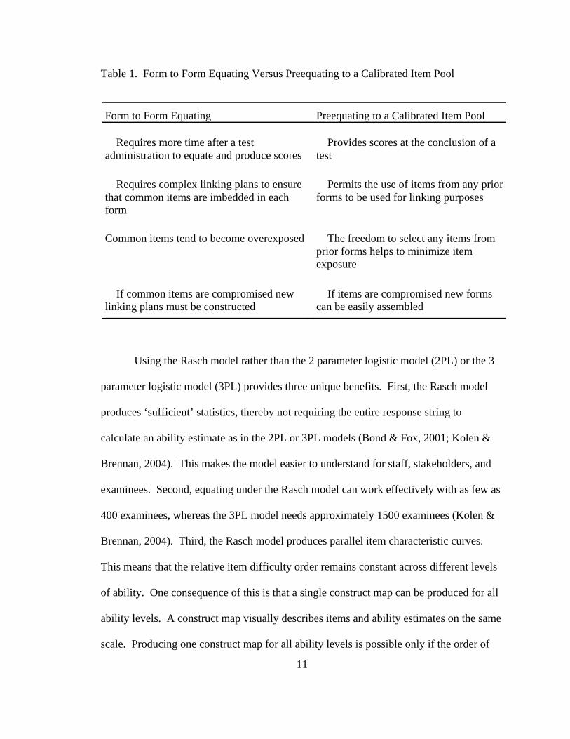
control of item exposure (Table 1). The flexibility in test assembly is made possible

because common items for a new form can be sampled from any prior forms in the pool

and joined together in a new form (Kolen & Brennan, 2004). This flexibility maximizes

control over item exposure. In the event that items are exposed, preequating to a

calibrated item pool provides flexibility in assembling new forms. As previously

mentioned, preequating allows for the reporting of test scores immediately following a

test administration, which is ideal for fixed length computer based tests (CBT). In

contrast to computer adaptive testing, preequating permits forms to be assembled and

screened by subject matter experts to ensure that items do not interact in unexpected

ways. Preequating with a calibrated item pool is an ideal equating solution for fixed

length CBTs.

11

Table 1. Form to Form Equating Versus Preequating to a Calibrated Item Pool

Form to Form Equating Preequating to a Calibrated Item Pool Requires more time after a test administration to equate and produce scores

Provides scores at the conclusion of a test

Requires complex linking plans to ensure that common items are imbedded in each form

Permits the use of items from any prior forms to be used for linking purposes

Common items tend to become overexposed The freedom to select any items from

prior forms helps to minimize item exposure

If common items are compromised new linking plans must be constructed

If items are compromised new forms can be easily assembled

Using the Rasch model rather than the 2 parameter logistic model (2PL) or the 3

parameter logistic model (3PL) provides three unique benefits. First, the Rasch model

produces ‘sufficient’ statistics, thereby not requiring the entire response string to

calculate an ability estimate as in the 2PL or 3PL models (Bond & Fox, 2001; Kolen &

Brennan, 2004). This makes the model easier to understand for staff, stakeholders, and

examinees. Second, equating under the Rasch model can work effectively with as few as

400 examinees, whereas the 3PL model needs approximately 1500 examinees (Kolen &

Brennan, 2004). Third, the Rasch model produces parallel item characteristic curves.

This means that the relative item difficulty order remains constant across different levels

of ability. One consequence of this is that a single construct map can be produced for all

ability levels. A construct map visually describes items and ability estimates on the same

scale. Producing one construct map for all ability levels is possible only if the order of

12

item responses is consistent across ability levels, and the order of respondents remains the

same for all item responses (Wilson, 2006). For these reasons, the Rasch model is an

attractive model to use for criterion referenced tests that have small sample sizes of 500

examinees.

While the Rasch model does provide many benefits, it does come with a high

price tag. The Rasch model assumes equivalent item discriminations and items with little

or no guessing (Hambleton & Swaminathan, 1985). Considerable resources can be

expended during the test development and item writing process to create items that

conform to these assumptions. The cost of implementing Rasch preequating could be

reduced considerably if preequating was shown to be robust to moderate violations of

these assumptions. Cost concerns aside, if the violations of the assumptions are too

severe, Rasch preequating will likely not produce better results than equating using

conventional methods.

Generally, IRT equating methods produce less equating error (Kolen & Brennan,

2004) than conventional CTT equating methods; however, IRT methods require strong

assumptions that cannot always be satisfied (Livingston, 2004). As a result, equating

studies are necessary to test the robustness of IRT equating methods to violations of IRT

assumptions in a given testing context (Kolen & Brennan, 2004).

Statement of the Problem

There are three major threats to the viability of preequating to a calibrated item

pool using the Rasch model: violations of Rasch model assumptions, nonequivalence of

13

groups, and item parameter bias in piloted items. The Rasch model assumes

unidimensionality, item response independence, no guessing, and equivalent item

discriminations (Hambleton & Swaminathan, 1985). Prior research has shown that

preequating is vulnerable to multidimensionality (Eignor & Stocking, 1986). The

probable cause for preequating error is the presence of bias in the item parameter

estimates caused by the violation of the assumption of item independence (Kolen &

Brennan, 2004). It is well known that multidimensionality can bias item parameter

estimates (Li & Lissitz, 2004). Eignor and Stocking (1986) discovered positive bias in

difficulty parameter estimates under multidimensional data. This effect was magnified

when population nonequivalence interacted with multidimensionality (Eignor &

Stocking, 1986). It is rare for any test to be completely free of multidimensionality (Lee

& Terry, 2004). Multidimensionality is especially common among professional

certification and licensing exams where all the vital job duties of a profession are often

included in one test blueprint.

The second major threat to the viability of Rasch preequating is population

nonequivalence. The Rasch model has been criticized in years past for not working

effectively when group ability differences are large (Skaggs & Lissitz, 1986; Williams,

Pommerich, & Thissen, 1998). However, Linacre and Wright (1998), DeMars (2002)

and more recently Pomplun, Omar, and Custer (2004) obtained accurate item parameter

estimates when scaling vertically, i.e. placing scores from different educational grade

levels onto the same scale. These researchers used the Joint Maximum Likelihood

Estimation (JMLE) method. The results that favored the Rasch model were based on

data that mostly satisfied the model assumptions. It is unclear how these results would

14

have differed if the assumptions were mildly or moderately violated. If Rasch

preequating is to be used with groups that differ moderately or substantially in ability, it

will need to be robust to mild violations of assumptions, and to be cost-effective, robust

to moderate violations.

The third major threat to the viability of Rasch preequating is the threat of

obtaining biased pilot item parameter estimates. Preequating to a calibrated item bank

requires that items are piloted to obtain item parameter estimates. This can be achieved

by administering intact pilot tests to representative groups of examinees, or placing

subsets of pilot items in operational exams. This study is focusing on the latter case,

because placing pilot items in operational forms is very conducive to computer based

testing. Kolen and Brennan (2004) warn of the risk that piloted items may become biased

during estimation because they are not calibrated within the context of an intact test form.

Prior studies have demonstrated preequating’s sensitivity to item parameter instability

(Du, Lipkins, & Jones, 2002) and item context effects (Kolen & Harris, 1990). Item

context effects can be controlled to some degree by keeping common items in fixed

locations across forms (Kolen & Brennan, 2004) and selecting stable items (Smith &

Smith, 2004) that are resistant to context effects. They can also be minimized by piloting

content representative sets of items rather than isolated items, which keeps the factor

structure constant across all the calibrations of piloted items (Kolen & Brennan, 2004).

Another factor that may contribute to item parameter bias is the method used for

calibrating items. This study contrasted fixed parameter calibration (FPC) to the

commonly used method of separate calibration and linking with the Stocking and Lord

method (SCSL). FPC holds previously estimated item parameters constant and uses a

15

parameter estimation method, in this case Joint Maximum Likelihood, to estimate item

parameter estimates for the new items. In contrast, SCSL finds linking constants by

minimizing the difference between estimated Test Characteristic Curves (TCCs). In IRT,

TCCs are curves that describe the relationship between thetas and true scores. FPC is one

method that can work under a preequating approach that can potentially simplify the

calibration procedures because it does not require a separate linking step. It can simplify

the calibration process, only if convergence problems reported by some (Kim, 2006) are

not too common. Much of the prior research on FPC has focused on the software

programs PARSCALE (Jodoin, Keller, & Swaminathan, 2003; Prowker, 2006), Bilog

MG, Multilog, and IRT Code Language (ICL) software (Kim, 2005). All of these

software programs implement Marginal Maximum Likelihood Estimation (MMLE)

through the Expectation Maximization algorithm. FPC has been shown to work less

effectively under nonnormal latent distributions (Paek & Young, 2005; Kim, 2005; Li,

Tam, & Tompkins, 2004) when conducted with MMLE. Very little, if any, published

research can be found on FPC in conjunction with Bigsteps/Winsteps which uses a Joint

Maximum Likelihood Estimation method. It is unclear how well FPC will perform under

a JMLE method when groups differ in ability and are not normally distributed. Data

from criterion referenced tests often exhibit ceiling or floor effects, which produce

skewed distributions. FPC would be the most attractive estimation method to work in a

preequating design because of its ease of use; however, it is not known how biased its

estimates will be under mild to moderate levels of population nonequivalence and model

data misfit.

This study was conducted to evaluate the performance of Rasch preequating to a

16

calibrated item pool under conditions that pose the greatest threat to its performance:

multidimensionality, population nonequivalence, and item parameter misfit. Using FPC

in conjunction with preequating would lower the costs and complexity of preequating;

however, prior research has not established whether or not FPC will produce unbiased

estimates under violated assumptions when estimated with JMLE.

Purpose of the Study

The purpose of this study was to compare the performance of Rasch true score

preequating methods to conventional linear equating under violated Rasch assumptions

(multidimensionality, guessing, and nonequivalent discrimination parameters) and

realistic levels of population nonequivalence. The outcome measures of interest in this

study included random and systematic error. In order to measure systematic error, a

simulation study was performed. A simulation study was chosen because simulations

provide a means of defining a criterion equating function from which bias can be

estimated. The main goal of this study was to delineate the limits of Rasch true score

preequating under the realistic test conditions of multidimensionality, population

nonequivalence, item discrimination nonequivalence, guessing, and their interactions for

criterion referenced tests. A secondary purpose was to compare FPC to the established

method of separate calibration and linking with SCSL.

17

Research Questions

1. Do Rasch true score preequating methods (FPC and SCSL) perform better than

postequating methods (identity and linear equating) when the IRT assumption of

unidimensionality is violated, but all other IRT assumptions are satisfied? As for the

preequating methods, does the FPC method perform at least as well as the SCSL method

under the same conditions?


postequating methods (identity and linear equating) when populations are

nonequivalent, and IRT model assumptions are satisfied? Does the FPC method perform

at least as well as the SCSL method under the same conditions?


postequating methods (identity and Linear equating) when the Rasch model assumption

of equivalent item discriminations is violated, but populations are equivalent and other

IRT model assumptions are satisfied? Does the FPC method perform at least as well as

the SCSL method under the same conditions?


postequating methods (identity and linear equating) when the Rasch model assumption of

no guessing is violated, but populations are equivalent and other IRT model assumptions

18

are satisfied? Does the FPC method perform at least as well as the SCSL method under

the same conditions?

5. How does Rasch preequating perform when response data are simulated with a three

parameter, compensatory two dimensional model, the assumption of equivalent item

discriminations is violated at three levels (mild, moderate, severe violations), the

assumption of no guessing is violated at three levels (mild, moderate, severe), population

non-equivalence is manipulated at three levels (mild, moderate, severe) and the

unidimensional assumption is violated at three levels (mild, moderate, severe)?

a. What are the interaction effects of multidimensionality, population non-

equivalence, nonequivalent item discriminations, and guessing on random

and systematic equating error?

b. At what levels of interaction does Rasch preequating work less effectively

than identity equating or linear equating?

c. How does FPC compare to SCSL in terms of equating error under the

interactions?

d. Does equating error accumulate across four equatings under the

interactions?

Importance of the Study

Methods do exist for estimating random error in equating; however,

overreliance on estimates of random error to the neglect of systematic error can give a

false sense of security since bias may pose a substantial threat to equated scores (Angoff,

19

1987; Kolen & Brennan, 2004). When IRT assumptions are violated, it is probable that

systematic error will appear in the item parameter estimates (Li & Lissitz, 2000) which

will likely increase equating error (Kolen & Brennan, 2004). Without knowing how

sensitive Rasch preequating methods are to sources of systematic error such as violated

assumptions, practitioners may underestimate the true amount of total error in the

method.

Understanding the interaction of multidimensionality and ability differences is

important to many testing applications including the study of growth, translated and

adapted tests, and certification tests that administer tests to professional or ethnic groups

that differ in ability. For instance, many educational testing programs designed to

measure Annual Yearly Progress (AYP) utilize IRT equating. Estimates of AYP are only

as accurate as the equating on which they are based. Much of the prior research on FPC

has focused on Bilog MG, Multilog, Parscale, and ICL. There is little, if any, published

research testing the accuracy of IRT preequating when performed with

Bigsteps/Winsteps. Since Bigsteps and Winsteps are popular software programs

worldwide for implementing the Rasch model, many groups could benefit from the

preequating design if it is found to be robust to violations.

FPC potentially is less expensive to use than other item calibration strategies (Li,

Tam, & Tomkins, 2004). This is due to the fact that FPC does not require a separate item

linking process. FPC is an increasingly popular method because of its convenience and

ease of implementation (Li, Tam, & Tomkins, 2004). A number of states such as Illinois,

New Jersey, and Massachusetts, use FPC to satisfy No Child Left Behind (NCLB)

requirements to measure AYP (Prowker, 2005). Professional certification companies use

20

FPC in conjunction with preequating. Few studies have examined FPC with

multidimensional tests, which are common in this context. Computer adaptive testing

programs use FPC (Ban, Hanson, Wang, Yi, & Harris, 2001). Previous studies have

demonstrated FPC’s vulnerability to nonnormal, nonequivalent latent distributions when

parameters are estimated using MMLE. FPC produces biased item parameter estimates

when the priors are misspecified (Paek & Young, 2006). However, I am not aware of

any research to date that has examined how well FPC performs under a JMLE method

with nonnormal, nonequivalent latent distributions.

Definition of Terms

Alternate forms- Alternate forms measure the same constructs in similar ways, share the

same purpose, share the same test specifications, and are administered in a

standardized manner. The goal of creating alternate forms is to produce scores

that are interchangeable. In order to achieve this goal, alternate forms often have

to be equated. There are three types of alternate forms: parallel forms, equivalent

forms, and comparable forms, the latter two require equating (AERA, APA,

NCME, 1999).

Calibration- In linking test score scales, the process of setting the test score scale,

including mean, standard deviation, and possibly shape of the score distribution,

so that scores on a scale have the same relative meaning as scores on a related

scale (AERA, APA, NCME, 1999). In IRT item parameter estimation, calibration

refers to the process of estimating items from different test forms and placing the

21

estimated parameters on the same theta scale. Once item parameters have been

estimated and placed on the same scale as a base form or item bank, the item

parameters are said to be calibrated (Kolen & Brennan, 2004).

Common Item Nonequivalent Groups Design- Two forms have one set of items in

common. Different groups (nonequivalent groups) are given both tests. The

common items are used to link the scores from the two forms. The common items

can be internal, which are used in the arriving at the raw score or external to the

test, which are not used in determining the raw score.

Comparable forms- Forms are highly similar in content, but the degree of statistical

similarity has not been demonstrated (AERA, APA, NCME, 1999).

Equating- The process of placing scores from alternate (equivalent) forms on a common

scale. Equating adjusts for small differences in difficulty between alternate forms

(AERA, APA, NCME, 1999). “Equating adjusts for differences in difficulty, but

not differences in content” (Kolen & Brennan, 2004).

Equating data collection design- An equating data collection design is the process by

which test data are collected for equating, such that ability differences between

groups can be controlled (Kolen & Brennan, 2004).

Equipercentile equating- Equipercentile equating produces equivalent scores with

equivalent groups by assuming the scores associated with percentiles are

equivalent across forms (Kolen & Brennan, 2004).

Equivalent forms (i.e., equated forms)- Small dissimilarities in raw score statistics are

22

compensated for in the conversions to derived scores or in form-specific norm

tables. The scores from the equated forms share a common scale (AERA, APA,

NCME, 1999).

External- In the context of common item nonequivalent groups design, common (anchor)

items that are used to equate test scores, but that are not used to calculate raw

scores for the operational test (Holland & Dorans, 2006).

Identity equating- This equating method assumes that scores from two forms are already

on the same scale. Identity equating is appropriate when alternate test forms are

essentially parallel.

Internal- In the context of common item nonequivalent groups design, common (anchor)

items that are used to equate and to score the tests (Holland & Dorans, 2006).

IRT preequating- See preequating

Item Characteristic Curve (ICC)- In IRT, an ICC relates the theta parameter to the

probability of a positive response to a given item.

Item preequating- See preequating

Item Response Theory (IRT)- A family of mathematical models that describe the

relationship between performance on items of a test and level of ability, trait, or

proficiency being measured usually denoted θ. Most IRT models express the

relationship between an item mean score and θ in terms of a logistic function

which can be represented visually as an Item Characteristic Curve (AERA, APA,

23

NCME, 1999).

Linear equating- Linear equating uses a linear formula to relate scores of two forms. It

accomplishes equating by assuming z scores across forms are equivalent among

equivalent groups.

Linking (i.e., linkage)- Test scores and item parameters can be linked. When test scores

are linked, multiple scores are placed on the same scale. All equating is linking,

but not all linking is equating. When linking is performed on scores derived from

test forms that are very similar in difficulty, then this type of linking is considered

an equating. When linking is done to tests that differ in content or difficulty or if

the populations of the groups differ greatly in ability, then this type of linkage is

not considered an equating (Kolen & Brennan, 2004). When item parameter

estimates are linked, parameters are placed on the same calibrated theta scale.

Kolen and Brennan also refer to this process as item preequating (2004).

Mean equating- Mean equating assumes that the relationship between the mean raw

scores of two forms given to equivalent groups defines the equating relationship

for all scores along the score scale.

Parallel forms (i.e., essentially parallel)- Test versions that have equal raw score means,

equal standard deviations, equal error structures, and equal correlations with other

measures for any given population (AERA, APA, NCME, 1999).

Preequating- The process of using previously calibrated items to define the equating

function between test forms prior to the actual test administration.

24

Random equating error- see standard error of equating.

Scaling- Placing scores from two or more tests on the same scale (Linn, 1993). See

linking.

Standard error of equating- The standard error of equating is defined as the standard

deviation of equated scores over hypothetical replications of an equating

procedure in samples from a populations of examinees. It is also an index of the

amount of equating error in an equating procedure. The standard error of

equating takes the form of random error, which reduces as sample size increases.

In contrast, systematic error will not change as sample size increases.

Systematic equating error- Equating error that is not affected by sample size, usually

caused by a violation of a statistical assumption of the chosen equating method or

psychometric model.

Test Characteristic Curve (TCC)- In IRT, a TCC relates theta parameters to true scores.

Test specifications- Formally defined statistical characteristics that govern the assembly

of alternate test forms.

Transformation- See linking

True Score- An examinee’s hypothetical mean score of an infinite number of test

administrations from parallel forms. If the reliability of a form was perfect, then the true

score and raw scores are equivalent. As reliability reduces, true scores and raw scores

diverge. Given the relationship between raw scores, true scores, and test reliability,

25

regression can be used to estimate the true score within a Classical True Score theory

point of view. Item Response Theory also provides models that can estimate true scores.

26

CHAPTER TWO

LITERATURE REVIEW

Chapter Two is divided into five sections. The first section provides a brief

overview of the relationship between linking and equating. Section one clarifies many

concepts that are closely related to equating but differ in important ways, giving a needed

context to the remainder of the chapter. The second section provides a review of three

data collection designs for equating methods. Reviewing all three designs provide the

historical and theoretical basis for the design used in this study. The third section

presents the equating methods utilized in this study, including formulas and procedures.

The fourth section reviews the factors that affect equating effectiveness, including

findings and gaps in the literature concerning preequating. The final section summarizes

the literature review.

Equating in the Context of Linking

Equating is a complex and multifaceted topic. Equating methods and designs have

been developed and researched intensely for many decades. Efforts have been made in

years past to better delineate equating from other closely related concepts. Currently,

there are at least two classification schemes that attempt to organize equating and related

27

topics. The first is the Mislevy/Linn Taxonomy (Mislevy, 1992). The second is a

classification scheme adopted by the National Research Council for their report

Uncommon Measures: Equivalence and linkage among educational tests (Feuer,

Holland, Green, Bertenthal, & Hemphill, 1999). Holland and Dorans present an

introduction to linking and equating in the latest edition of Educational Measurement

which provides a useful summary of the many concepts shared in the two classification

schemes (Holland & Dorans, 2006).

Holland and Dorans divide linking into three types: prediction, scale alignment,

and test equating. They define a link as a transformation of a score from one test to

another (Holland & Dorans, 2006). What follows is a brief overview of their

classification scheme. The reader is encouraged to read the full article for a more

complete description of the scheme.

Prediction

The purpose of prediction is to predict Y scores from X scores. The relationship

between form Y and form X scores is asymmetric. For instance, a regression equation

does not equal its inverse. Typically, observed scores are used to predict expected scores

from one test to a future test. An example of an appropriate use of predicting observed

scores is predicting future SAT scores from PSAT scores (Holland & Dorans, 2006). In

addition to predicting Y observed scores from form X scores, one can also predict Y true

scores from form X scores. Kelley provided a formula to predict form Y true scores from

form Y observed scores. Later this formula was modified to predict form Y true scores

28

from form X observed scores (Holland & Dorans, 2006).

Scale Alignment

When form X and Y measure different constructs or are governed by different test

specifications scale aligning can be employed to place the scores onto the same scale.

When the scores from form Y and X come from the same population, aligned scores are

referred to as comparable scores, comparable measures (Kolen & Brennan, 2004), or

comparable scales (Holland & Dorans, 2006). When scores from form Y and X come

from different populations the terms anchor scaling (Holland & Dorans, 2006), statistical

moderation, or 'distribution matching' (Kolen & Brennan, 2004) are used. An example of

statistical moderation is an attempt to link translated or adapted tests. Even if the

translated test consists of the same items as those in the original language, the constructs

may not be equivalent across cultures. In addition, the abilities of language groups

probably differ (Kolen & Brennan, 2004).

Vertical scaling is a type of scale alignment that is performed when constructs and

reliabilities of form X and Y scores are similar, but the groups being linked come from

different populations or are very different in ability (Kolen & Brennan, 2004). The most

common use of vertical scaling is placing the scores of students across many grades onto

the same scale. It should be noted that it is common for researchers to use the phrase

'vertical equating' to describe vertical scaling. Tests designed for different grades that

share common items, would not qualify as equating, because a requirement of equating is

that the forms should be made as similar as possible (Kolen & Brennan, 2004). Equating

29

adjusts for small differences in form difficulty (AERA, APA & NCME, 1999). Tests

designed for vertical scaling are often assembled to be very different in difficulty to

match the ability levels of various groups.

When form X and Y scores measure similar constructs, have similar reliabilities,

similar difficulties, and the same population of examinees, but different test

specifications, then the only appropriate type of scale aligning that can be performed is a

concordance (Holland & Dorans, 2006). Concordances can be made of two similar tests

that were not originally designed to be equated. A common example of this type of scale

alignment is relating SAT scores to ACT scores. It is important to note that none of the

examples of scale aligning presented here produce equivalent scores, a designation

reserved for test equating.

Test Equating

The Standards for Educational and Psychological Testing define equating as,

“The process of placing scores from alternate forms on a common scale. Equating adjusts

for small differences in difficulty between alternate forms (AERA, APA, NCME, 1999)”.

In order for the results of an equating procedure to be meaningful a number of

requirements must be satisfied. The requirements of equated scores include symmetry,

equal reliabilities, interchangeability or equity, similar constructs, and population

invariance (Angoff, 1971; Kolen & Brennan, 2004; Holland & Dorans, 2006).

Symmetry refers to the idea that the equating relationship is the same regardless if

one equates from form X to form Y or vice versa. This property supports

30

interchangeability, the idea that an examinee's score should not depend on which form

he/she takes. It should be noted that these forms should be interchangeable across time or

location. If the items in an item bank become more and more discriminating over time,

there is a possibility that test forms constructed from such items may become more and

more reliable. Ironically, improving a test too much may work against equating to some

extent. The implication to testing programs that plan to equate forms across many years

is to ensure that the initial item pool is robust enough to support a high level of reliability,

because the reliability of the test should not improve or degrade.

Interchangeability is also supported by the concept of equal reliabilities, for if one

equated form had more or less reliability, the performance of the examinee may depend

on which form is taken. For instance, lower performing examinees may benefit from less

reliable tests (Holland & Dorans, 2006).

Population invariance requires that the equating relationship hold across

subgroups in the population, otherwise, subgroups could be positively or negatively

affected. The concern in population invariance of equating functions usually focuses on

ethnic groups who perform below the majority group (De Champlain, 1996).

Finally, similar constructs are required of two equated forms to ensure that the

meaning of scores is preserved. This requirement implies that equating is intolerant of

changing content. If the content of a test changes too much, a new scale and cut score

may have to be defined. Some other type of linking, other than equating, could then be

used to relate the new scale to the prior scale.

There are a number of requirements of equating that are not altogether required of

other forms of linking. Equating requires that forms are similar in difficulty, with similar

31

levels of reliability, high reliability, similar constructs, proper quality control, and

identical test specifications (Dorans, 2004; Kolen & Brennan, 2004).

A distinction should be made between vertical and horizontal equating.

Horizontal equating refers to equating that occurs between groups of very similar ability,

while vertical equating refers to equating that occurs between groups that have different

abilities. An example of horizontal equating is the equating of scores from a well defined

population, such as graduates from a specific graduate school program. Such examinees

are expected to be similar in ability. An example of vertical equating is the equating of

forms from a majority group and a minority group, in which the minority group has a

different ability distribution than the majority group.

Summary of Linking and Equating

Equating is distinguished from other forms of linking in that equating is the most

rigorous type of linking, requiring forms similar in difficulty, with similar levels of

reliability, high reliability, similar constructs, and identical test specifications (Dorans,

2004). Equated forms strive to exemplify the ideal psychometric qualities of symmetry,

equal reliabilities, interchangeability, similar constructs, and population invariance.

When these ideals are met, the goal of equating is achieved: test scores from two forms

are interchangeable (Von Davier, Holland, & Thayer, 2004). Kolen and Brennan (2004)

stress that equating cannot adjust for differences in content, only differences in difficulty.

Vertical scaling and vertical equating are similar in that they both relate scores from

groups that differ in ability. However, vertical scaling is distinguished from vertical

32

equating in that equating relates forms that are very similar in difficulty and vertical

scaling relates forms that are very different in difficulty. What follows next is an

explanation of the data collection designs that can be used for equating.

Data Collection Designs for Equating

As mentioned previously, there are a number of ways to prevent the confounding

of group ability and test form difficulty. An equating data collection design is the process

by which data are collected to ensure that group ability and test form difficulty are

disconfounded, allowing forms to be equated (Holland & Dorans, 2006). In the literature

one can find at least three designs commonly employed to collect data for equating

(Skaggs & Lissitz, 1986). The common designs include the random groups, the single

group with counter balancing, and the common item nonequivalent group design. A less

commonly cited design is the common item equating to an IRT calibrated item pool

(Kolen & Brennan, 2004). Each design separates ability from form difficulty in different

ways.

Random Groups Design

The random groups design achieves equivalent group abilities through the use of

random assignment of forms to examinees. If the sample of examinees is large enough, it

can be assumed that the difference between scores on the forms is caused by form

differences. This design accommodates more than two forms, but requires large sample

33

sizes of at least 1500 examinees (Kolen & Brennan, 2004). The design requires that all

forms to be equated are administered simultaneously. If cheating is a concern, equating

more than two forms simultaneously is undesirable because of item exposure (Kolen &

Brennan, 2004). It is not an appropriate method if forms are to be equated across time.

Single Groups with Counterbalancing Design

Single groups with counterbalancing is a data collection design that requires each

examinee to take the base form and the new form. Examinees are randomly assigned to

one of two groups. Group One receives form X and then form Y. Group two receives

form Y and then form X. This is referred to as counterbalancing and is used to control for

order effects. Mean, linear, or equipercentile equating methods can then be used to

isolate the differences caused by form difficulty (Kolen & Brennan, 2004; Holland &

Dorans, 2006). The major drawback to this design is the fact that each examinee is

required to take two test forms. Not only is this inconvenient and time consuming for

examinees, but item exposure increases.

Common Item Designs

The final two methods employ common items rather than common persons

between forms. The CINEG, also known as, the nonequivalent group with anchor test

(NEAT), is the most commonly used design. A lesser used design is known as the

common item equating to a calibrated item pool. The two designs differ in that the

34

former links two or more forms, while the latter equates new forms to a calibrated item

bank. Both methods use the same logic that the single group design employs, except that

rather than requiring all examinees to complete all forms, examinees are required to

complete one form and a mini version of the other form. In such equating designs, the

mini test is used to predict scores on the entire form, and then mean, linear, or

equipercentile methods are used to estimate differences caused by form difficulty

(Holland & Dorans, 2006). IRT methods require the linking of items on a single theta

calibrated scale through the use of common items. Because all the items are calibrated to

the same scale, common items from any prior form can be used to link new forms to the

entire pool of items rather than to just a prior form (Kolen & Brennan, 2004). This last

design, common item to a calibrated item pool, permits preequating.

Equating Methods

This section will focus on CINEG equating methods that are relevant to samples

sizes of less than 500. This includes identity equating, linear equating, and preequating

with the Rasch model. There are many other methods of CINEG equating that are not

reviewed in this study. Mean equating, conventional equipercentile methods, IRT

observed score equating, as well as Kernel equating are also possible methods that could

be employed with a CINEG data collection design. However, all of these methods,

except for mean equating, require sample sizes that exceed the sample sizes being

investigated by this study (Kolen & Brennan, 2004). Identity equating and linear

equating will be used in this study primarily as criteria to help evaluate the performance

35

of preequating with the Rasch model. Since these methods are not the primary focus of

this study the description of these methods will be kept brief. Emphasis will be placed on

IRT preequating methods. The reader can find an excellent presentation of identity and

linear equating methods in Kolen and Brennan's Test Equating, Scaling, and Linking

(2004).

Identity Equating

Identity equating defines a score on a new form X to be equivalent to the same

score on the base form Y. For instance, a score of 70 on form X would equal a score of

70 on form Y. In some instances identity equating will produce less equating error than

other types of equating. For this reason, identity equating is often used as a baseline

method to compare the effectiveness of other methods (Bolt, 2001; Kolen & Brennan,

2004). Other equating methods should not be used unless they produce less equating

error than the identity function (Kolen & Brennan, 2004). If the scale is equal in

difficulty all along the scale, then identity equating equals mean and linear equating.

However, as test forms become less parallel other methods will produce less error than

the identity method. In some contexts, the term preequating is used to refer to tests that

have been assembled to be parallel. Then identity equating is used to relate scores. For

practical purposes, identity equating is the same as not equating.

36

Linear Equating

This section describes general linear equating under the single groups with

counter balancing design and then provides a brief description of linear equating used in

CINEG designs. There are a variety of ways to use common items in linear equating

methods, including “chained equating” and “conditioning on the anchor” (Livingston,

2004). Livingston (2004) explains that chained equating operates by linking scores on

the new form to scores from the common item set, and then linking scores from the

common item set to the base form. Conditioning on the anchor uses the scores from the

common item set to predict unknown parameters in a ‘synthetic’ group which are then

used as if they were observed for equating (Livingston, 2004). What follows is a

description of the general linear formula used in this procedure.

The general linear transformation is defined by setting z scores equal for forms X

and Y such that

(x-μ(X))/σ(X) = (y-μ(Y))/σ (Y) (2.1)

Where x = a raw score on a new form X,

μ(X) = is the mean score of form X,

σ(X) = the standard deviation of form X,

y = a raw score on the base form Y,

μ(Y) = is the mean score of form Y, and

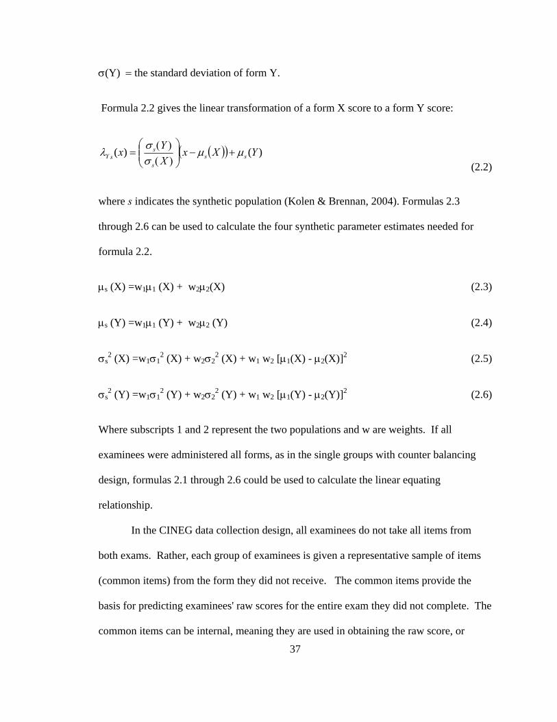
37

σ(Y) = the standard deviation of form Y.

Formula 2.2 gives the linear transformation of a form X score to a form Y score:

( )( ) )()( YXxXYx ss

s

ssY μμ

σσλ +−⎟⎟

⎠

⎞⎜⎜⎝

⎛)()(

= (2.2)

where s indicates the synthetic population (Kolen & Brennan, 2004). Formulas 2.3

through 2.6 can be used to calculate the four synthetic parameter estimates needed for

formula 2.2.

μs (X) =w1μ1 (X) + w2μ2(X) (2.3)

μs (Y) =w1μ1 (Y) + w2μ2 (Y) (2.4)

σs2 (X) =w1σ1

2 (X) + w2σ22 (X) + w1 w2 [μ1(X) - μ2(X)]2 (2.5)

σs2 (Y) =w1σ1

2 (Y) + w2σ22 (Y) + w1 w2 [μ1(Y) - μ2(Y)]2 (2.6)

Where subscripts 1 and 2 represent the two populations and w are weights. If all

examinees were administered all forms, as in the single groups with counter balancing

design, formulas 2.1 through 2.6 could be used to calculate the linear equating

relationship.

In the CINEG data collection design, all examinees do not take all items from

both exams. Rather, each group of examinees is given a representative sample of items

(common items) from the form they did not receive. The common items provide the

basis for predicting examinees' raw scores for the entire exam they did not complete. The

common items can be internal, meaning they are used in obtaining the raw score, or

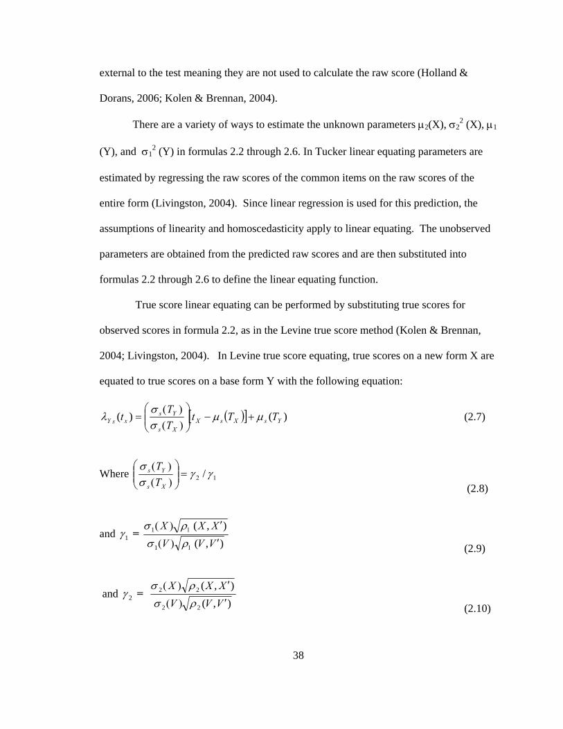
38

external to the test meaning they are not used to calculate the raw score (Holland &

Dorans, 2006; Kolen & Brennan, 2004).

There are a variety of ways to estimate the unknown parameters μ2(X), σ22 (X), μ1

(Y), and σ12 (Y) in formulas 2.2 through 2.6. In Tucker linear equating parameters are

estimated by regressing the raw scores of the common items on the raw scores of the

entire form (Livingston, 2004). Since linear regression is used for this prediction, the

assumptions of linearity and homoscedasticity apply to linear equating. The unobserved

parameters are obtained from the predicted raw scores and are then substituted into

formulas 2.2 through 2.6 to define the linear equating function.

True score linear equating can be performed by substituting true scores for

observed scores in formula 2.2, as in the Levine true score method (Kolen & Brennan,

2004; Livingston, 2004). In Levine true score equating, true scores on a new form X are

equated to true scores on a base form Y with the following equation:

[ ( )] )()( YsXsXXs

YsxsY TTt

TT

t μμσσ

λ +−⎟⎟⎠

⎞⎜⎜⎝

⎛)()(

=

(2.7)

Where 1/ γγσσ

2=⎟⎟⎠

⎞⎜⎜⎝

⎛)()(

Xs

Ys

TT

(2.8)

and 1γ = ),(),(

1

1

VVVXXX

′)(

′)(

1

1

ρσρσ

(2.9)

and 2γ = ),(),(

22

22

VVVXXX

′)(

′)(

ρσρσ

(2.10)

39

where ρ represents estimates for reliability, and V are the scores on common items. As

with any true score equating method, the equating relationship between true scores is

applied to observed raw scores.

Linear equating can falter when its assumptions are violated. For instance, linear

equating can falter if the regression line is curvilinear rather than linear. As with any

CINEG design if common items work inconsistently between groups, the equating error

of this method will increase quickly. Tucker linear equating is known to produce bias

whenever score reliabilities are less than 1. Levine true score equating corrects for this

bias (Livingston, 2004). Both the Tucker and Levine methods require scores from

common items that correlate highly with the test entire (Livingston, 2004). If group

ability differences are greater than .50 of a standard deviation problems can ensue (Kolen

& Brennan, 2004).

The ideal sample size for linear equating is at least 300 examinees (Kolen &

Brennan, 2004). The random error of linear equating is very susceptible to sample size,

so random error increases rapidly moving from the mean. There is evidence that linear

equating can work reasonably well with samples as low as 50, especially if the cut score

is close to the mean, if common item scores correlate highly with the overall test, and if

equating error does not propagate across links (Parshall, Houghton, & Kromrey, 1995).

Linear equating methods require relatively small samples in comparison to IRT and

equipercentile equating.

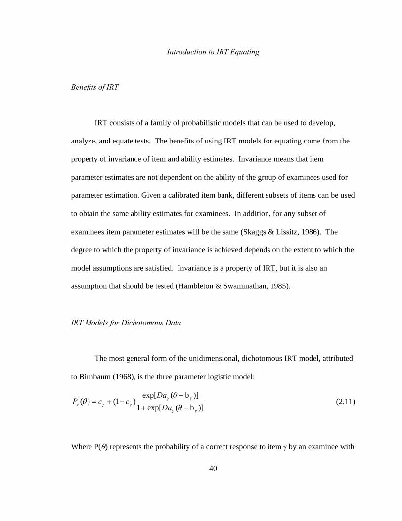
40

Introduction to IRT Equating

Benefits of IRT

IRT consists of a family of probabilistic models that can be used to develop,

analyze, and equate tests. The benefits of using IRT models for equating come from the

property of invariance of item and ability estimates. Invariance means that item

parameter estimates are not dependent on the ability of the group of examinees used for

parameter estimation. Given a calibrated item bank, different subsets of items can be used

to obtain the same ability estimates for examinees. In addition, for any subset of

examinees item parameter estimates will be the same (Skaggs & Lissitz, 1986). The

degree to which the property of invariance is achieved depends on the extent to which the

model assumptions are satisfied. Invariance is a property of IRT, but it is also an

assumption that should be tested (Hambleton & Swaminathan, 1985).

IRT Models for Dichotomous Data

The most general form of the unidimensional, dichotomous IRT model, attributed

to Birnbaum (1968), is the three parameter logistic model:

)]b(exp[1)]b(exp[

)1()(γγ

γγγγγ θ

θθ

− +

− −+=

DaDa

ccP (2.11)

Where P(θ) represents the probability of a correct response to item γ by an examinee with

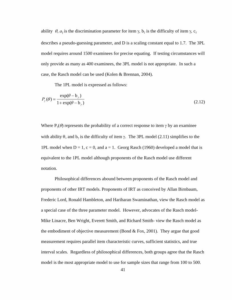
41

ability θ, aγ is the discrimination parameter for item γ, bγ is the difficulty of item γ, cγ

describes a pseudo-guessing parameter, and D is a scaling constant equal to 1.7. The 3PL

model requires around 1500 examinees for precise equating. If testing circumstances will

only provide as many as 400 examinees, the 3PL model is not appropriate. In such a

case, the Rasch model can be used (Kolen & Brennan, 2004).

The 1PL model is expressed as follows:

)bexp(1)bexp(

)(γ

γγ θ

θθ

− +

− =P

(2.12)

Where Pγ(θ) represents the probability of a correct response to item γ by an examinee

with ability θ, and bγ is the difficulty of item γ. The 3PL model (2.11) simplifies to the

1PL model when D = 1, c = 0, and a = 1. Georg Rasch (1960) developed a model that is

equivalent to the 1PL model although proponents of the Rasch model use different

notation.

Philosophical differences abound between proponents of the Rasch model and

proponents of other IRT models. Proponents of IRT as conceived by Allan Birnbaum,

Frederic Lord, Ronald Hambleton, and Hariharan Swaminathan, view the Rasch model as

a special case of the three parameter model. However, advocates of the Rasch model-

Mike Linacre, Ben Wright, Everett Smith, and Richard Smith- view the Rasch model as

the embodiment of objective measurement (Bond & Fox, 2001). They argue that good

measurement requires parallel item characteristic curves, sufficient statistics, and true

interval scales. Regardless of philosophical differences, both groups agree that the Rasch

model is the most appropriate model to use for sample sizes that range from 100 to 500.

42

IRT Equating Methods

Figure 1 presents the general steps required by IRT calibration and equating. Step

1 involves assembling a new test form in such a way that equating will be successful.

Step 2 involves estimating item parameters. This step assumes model data fit. The third

step referred to here as item linking, places estimated item parameters from both test

forms on the same scale. If theta estimates were being used for scoring purposes,

generally the next step would be to simply estimate thetas (Kolen & Brennan, 2004). No

other steps would be necessary to achieve score comparability; however, most testing

programs score tests using NC raw scores. Whenever NC scores are used rather than

thetas, step 4 is necessary (De Champlain, 1996). This step defines the equating function

between true or observed raw scores of the new form and the target form. Step 5 is the

process of relating equated raw scores obtained from Step 5 to primary scale scores.

Primary scale scores are the scores used for score reporting. During this step, conversion

tables are created that can be used by measurement staff and scoring programs for

reporting purposes.

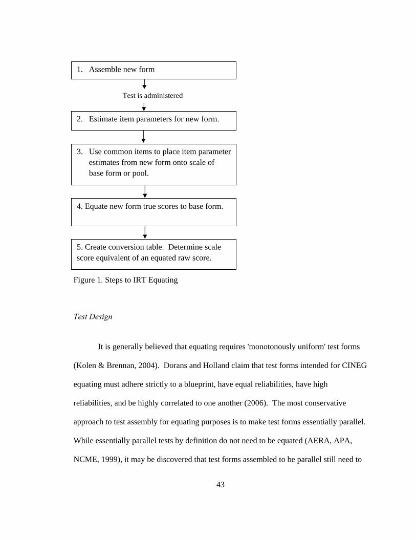
43

Figure 1. Steps to IRT Equating

Test Design

It is generally believed that equating requires 'monotonously uniform' test forms

(Kolen & Brennan, 2004). Dorans and Holland claim that test forms intended for CINEG

equating must adhere strictly to a blueprint, have equal reliabilities, have high

reliabilities, and be highly correlated to one another (2006). The most conservative

approach to test assembly for equating purposes is to make test forms essentially parallel.

While essentially parallel tests by definition do not need to be equated (AERA, APA,

NCME, 1999), it may be discovered that test forms assembled to be parallel still need to

1. Assemble new form

2. Estimate item parameters for new form.

3. Use common items to place item parameter estimates from new form onto scale of base form or pool.

4. Equate new form true scores to base form.

5. Create conversion table. Determine scale score equivalent of an equated raw score.

Test is administered

44

be equated due to item context effects. For instance, identical tests with shuffled items

are sometimes equated if items do not perform consistently (Hendrickson & Kolen, 1999;

Moses, Yang, & Wilson, 2007). Equating can also be performed on test forms that are

not essentially parallel (Kolen & Brennan, 2004). The standard practice of aligning Test

Information Functions (TIF) to the cut score to minimize error and matching Test

Characteristic Curves (TCC) of new forms to a target form largely address the test

assembly needs of preequating (Hambleton & Swaminathan, 1985). However, special

care must be given to the selection of common items.

There are many guidelines for selecting common items. Angoff (1971) claimed

that for linear equating not less than 20% of the items of a test should be anchor items.

IRT methods can achieve good results with fewer than 20% anchor items (Kim & Cohen,

1998). Hills, Subhihay, and Hirsch (1988) obtained good linking results with 10 items.

Raju, Edwards, and Osberg (1983) used 6 to 8 items successfully. Wingersky and Lord

(1984) used as few as 2 items with success. Forms to be equated should have content

representative common items (Kolen & Brennan, 2004), and have common items that

produce scores that correlate highly (r >.80) with the total test (Motika, 2003). It is also

necessary that the common items perform equally well between the groups and forms

intended to be equated. For this reason experts recommend that common items remain in

the same or similar position across forms to prevent item order and context effects (Cook

& Petersen, 1987).

45

Calibration and Linking Procedures

A variety of procedures can be performed to accomplish item calibration and item

linking including separate calibration with linking, concurrent calibration, or fixed

parameter calibration (FPC). Among users of IRT who use Marginal Maximum

Likelihood Estimation (MMLE) methods, the most common method used to complete

calibration and item linking (Figure 1, Steps 1, 2, and 3) is to estimate the item

parameters separately and then use an item linking method to place the item parameters

on the same scale. A variety of methods are available to perform this item linking

including Mean/Mean, Mean/Standard deviation, Stocking and Lord TCC method, and

the Haebara Method (Hambleton & Swaminathan, 1985; Kolen & Brennan, 2004). Any

of these methods will produce transformation constants λ and κ, which when entered into

equations

θ∗ = λθ + κ (2.13)

bγ*= λbγ + κ (2.14)

aγ*= aγ/λ (2.15)

will place the parameters onto the base scale. Many researchers report that the

characteristic curve based methods (Haebra and Stocking & Lord methods) usually

outperform the other methods (Tsai, Hanson, Kolen, & Forsyth, 2001; Hanson & Beguin,

2002; Kolen & Brennan, 2004). The Stocking and Lord method achieves the linking

46

constants by minimizing the differences between TCCs. SCSL has received consistently

better performance reviews than other linking methods (Kolen & Brennan, 2004; Hanson

& Beguin, 2002).

Another commonly used method, concurrent calibration, performs Steps 1, 2, and

3 during one run of IRT software. Concurrent calibration can be performed using a

common person or common items design (Smith & Smith, 2005). Because all the items

are estimated simultaneously, the items are already on the same scale and do not require

linking. If multiple forms are administered across time, more and more forms can be

added to the score matrix and concurrent calibration can be performed again. Linking

may still be used with concurrent calibration, if equating is necessary to relate groups of

concurrently calibrated forms across time. Prior research has shown that the parameter

estimates acquired over time increase in precision because the sample size for the

common items increase (Hanson & Beguin, 2002; Kim & Kolen, 2006). Potential

drawbacks to concurrent calibration include long convergence cycles and the risk of

nonconvergence.

FPC is a variation of concurrent calibration. FPC, also referred to as anchoring, is

a commonly used method among those who use Joint Maximum Likelihood Estimation

(JMLE). FPC is an attractive alternative to separate calibration with linking because it

can simplify the process of calibrating new items (Li, Tam, & Tomkins, 2004). In the

literature, FPC has many names including Pretest-item Calibration/scaling methods (Ban,

Hanson, Wang, Yi, & Harris, 2001), Fixed Common Item Parameter Equating (Jodoin,

Keller, & Swaminathan, 2003; Prowker, 2004), Fixed Common-Precalibrated Parameter

Method (Li, Tam, & Tompkins, 2004), Fixed Item Linking (Paek & Young, 2005), and

47

fixed parameter calibration (FPC) (Kim, 2006).

In FPC, the parameters of the common items in the new form are fixed to those of

the old form (Domaleski, 2006; Paek & Young, 2005; Li, Tam, & Tompkins, 2004; Kim,

2006). The remaining items are then allowed to be estimated using conventional

estimation algorithms. No linking is necessary at any stage of a testing program if FPC is

used.

A variety of software options and methods exist for estimating parameters. With

Bilog MG, multigroup concurrent calibration and FPC can be implemented using

MMLE. The advantage to multigroup estimation is that the distributions of the groups

are free to vary during the parameter estimation process. Multilog can also be used to

perform concurrent calibration with or without prior distributions specified using MMLE.

Bigsteps and Winsteps can perform FPC for the Rasch model using JMLE which does

not assume any prior distribution. Also, IRT Code Language (Hanson, 2002) can be used

to perform concurrent calibration or FPC procedures using MMLE.

IRT True Score Equating Procedures

Regardless of how calibration (Steps 2 and 3) is performed, if raw scores are

reported rather than thetas, equating is necessary to define the functional relationship

between NC scores across test forms (Step 4)(De Champlain, 1996). Either true or

observed scores can be the focal point of this equating process. In true score equating,

the TCC visually expresses the relationship between number correct true scores and

thetas. The expected true score (τ) for an examinee with ability of θj is given by,

48

)(1

j

n

P θτγ

γ∑=

= (2.16)

where Pγ is the probability of correctly answering item γ. In IRT true score equating, for

a given theta, a true score for form X is considered equivalent to a true score for form Y.

The form Y true score equivalent of a given true score on form X is

irty= (τx) = τy(τx−1 ), (2.17)

where τx−1 is the θj associated with true score τx,

τx equals a true score on form x,

τy equals a true score on form y.

Kolen and Brennan (2004) describe a three step process to equation 2.17. First,

specify a true score τx on form X. Second, find the θj that corresponds to that true score

(τx−1). Third, find the true score on Form Y, τy, that corresponds to that θj. In this way,

true scores from the two forms are associated through their common theta. The process

of finding the theta that corresponds to a true score, step 2, is achieved with an iterative

process such as the Raphson Newton method. Once this is completed, the functional

relationship between true scores of two forms is used to equate observed scores (De

Champlain, 1996; Hambleton & Swaminathan, 1985; Kolen & Brennan, 2004). A SAS

macro was developed to implement the Raphson Newton method (Appendix A).

Many large-scale testing programs employ some combination of the above

mentioned calibration, item linking, and true score equating procedures. This process

usually entails equating individual forms, one to another, after a test has been

49

administered. Much of the equating research over the past 20 years has focused on

equating relationships between forms after data have been collected during a test

administration. A handful of studies have been conducted on preequating. Some of the

studies reached opposing conclusions concerning the effectiveness of preequating. Fewer

still have examined equating with a calibrated item pool for fixed length tests. The next

section will review the procedures of IRT preequating, followed by a review of studies

that have investigated the performance of IRT preequating.

Preequating Procedures

Preequating can use any of the IRT CINEG estimation, item linking, and equating

procedures used in conventional IRT CINEG equating. IRT preequating differs from

postequating (Figure 1) in the sequence of steps. Figure 2 presents the steps of

preequating as it has been described by Kolen and Brennan (2004). The first step (1) is

assembling the form. The second step (2) is performing true score equating. The third

step (3) is the creation of conversion tables. After these steps are done, the test can be

administered, and scores, pass/fail decisions, and score reports can be provided

immediately upon completion of the test. Steps 1 through 3 are all that are necessary to

equate a test under the preequating model. For this reason preequating is especially

attractive to testing programs that use CBT or that have a small window of time to score,

equate, and report scores.

Steps 4 and 5 of preequating are performed simply to add new calibrated items to

the item pool. Step 4 involves estimating item parameters, and step 5 uses the common

50

items to place the pilot items onto the same scale as the calibrated item pool. Any of the

previously presented item calibration methods can be used to perform these steps.

It should be noted that some researchers have adopted the term ‘item preequating’

to describe steps 4 and 5 (De Champlain, 1996). In contrast, Kolen and Brennan’s (2004)

use of the term item preequating implies steps 1 through 5. For the purposes of this

study, I am using the term preequating to refer to steps 1 through 3, and item calibration

to refer to 4 and 5.

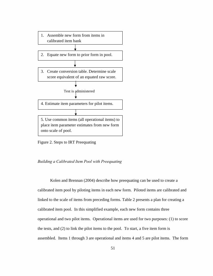
51

Figure 2. Steps to IRT Preequating

Building a Calibrated Item Pool with Preequating

Kolen and Brennan (2004) describe how preequating can be used to create a

calibrated item pool by piloting items in each new form. Piloted items are calibrated and

linked to the scale of items from preceding forms. Table 2 presents a plan for creating a

calibrated item pool. In this simplified example, each new form contains three

operational and two pilot items. Operational items are used for two purposes: (1) to score

the tests, and (2) to link the pilot items to the pool. To start, a five item form is

assembled. Items 1 through 3 are operational and items 4 and 5 are pilot items. The form

1. Assemble new form from items in calibrated item bank

2. Equate new form to prior form in pool.

3. Create conversion table. Determine scale score equivalent of an equated raw score.

4. Estimate item parameters for pilot items.

5. Use common items (all operational items) to place item parameter estimates from new form onto scale of pool.

Test is administered

52

is assembled (step 1) and data are collected. Item parameters are estimated (step 2) using

an IRT software program for the operational form (e.g., items 1 through 3). Then after

scoring (step 3) is complete, the pilot items are calibrated (step 4) and linked (Step 5) to

the operational items. The linked pilot items are then added to the calibrated item pool

(Step 6). Form 2 is then assembled consisting of items 3 through 7 (Step 1). True score

equating (Step 2) is then performed using the common items 3 - 5. Conversion tables are

made (Step 3) and form 2 is administered. Scores can be determined with the use of the

conversion tables. Some time after the tests have been scored, the piloted items can be

calibrated, linked, and added to the item bank (steps 4 through 6). Steps 1 through 6 can

be repeated as many times as necessary to build a calibrated item pool.

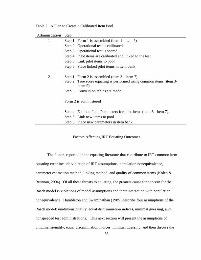
53

Table 2. A Plan to Create a Calibrated Item Pool

Administration Step 1 Step 1. Form 1 is assembled (item 1 - item 5) Step 2. Operational test is calibrated Step 3. Operational test is scored. Step 4. Pilot items are calibrated and linked to the test. Step 5. Link pilot items to pool Step 6. Place linked pilot items in item bank 2 Step 1. Form 2 is assembled (item 3 – item 7)

Step 2. True score equating is performed using common items (item 3- item 5).

Step 3. Conversion tables are made. Form 2 is administered Step 4. Estimate Item Parameters for pilot items (item 6 - item 7). Step 5. Link new items to pool Step 6. Place new parameters in item bank

Factors Affecting IRT Equating Outcomes

The factors reported in the equating literature that contribute to IRT common item

equating error include violation of IRT assumptions, population nonequivalence,

parameter estimation method, linking method, and quality of common items (Kolen &

Brennan, 2004). Of all these threats to equating, the greatest cause for concern for the

Rasch model is violations of model assumptions and their interaction with population

nonequivalence. Hambleton and Swaminathan (1985) describe four assumptions of the

Rasch model: unidimensionality, equal discrimination indices, minimal guessing, and

nonspeeded test administrations. This next section will present the assumptions of

unidimensionality, equal discrimination indices, minimal guessing, and then discuss the

54

issues of population nonequivalence, quality of common items, and calibration linking

method.

Assumption of Unidimensionality

Many studies have examined the robustness of IRT equating to violations of the

assumption of unidimensionality. The majority of these studies concluded that IRT

equating was robust to violations of IRT assumptions (Bogan & Yen, 1983; Camili,

Wang, & Fesq, 1995; Cook, Dorans, Eignor, & Petersen, 1985; Dorans & Kingston,

1985; Wang, 1985; Yen, 1984; Smith, 1996). However, most of these referenced studies

were performed with actual data using the 3PL model, a few on the 2PL model, and one

on the Rasch model. None of these studies examined IRT preequating.

A few studies have explicitly examined IRT Preequating with the 3PL model.

Stocking and Eignor (1986) found that when the assumption of unidimensionality was

violated the b parameters were overestimated, which led to substantial equating error.

Prior research on the American College Test (ACT) and the Scholastic Aptitude Test

(SAT) showed that preequating is sensitive to multidimensionality and item context

effects (Eignor, 1985; Kolen & Harris, 1990; Hendrickson & Kolen, 1999). Kolen and

Harris (1990) found that with the ACT Mathematics Test, preequating produced more

equating error than identity equating, which is equivalent to not equating at all. These

problems were so severe that the idea of preequating was abandoned for these programs.

The probable cause for equating error under multidimensionality is the presence of bias

in the item parameter estimates (Kolen & Brennan, 2004). Li and Lissitz reported the

55

presence of bias in item parameter estimates when data are not strictly unidimensional

(2004).

While there are many studies that cast doubt on the viability of IRT preequating

under multidimensionality, some studies have obtained favorable results with IRT

preequating under known multidimensional tests. The Law School Admissions Test

(LSAT) used a section preequating design with the 3PL model in the 1990s. A section

preequating design pilots items within test sections that are spiraled to achieve equivalent

groups during test administration. Concurrent calibration is then used to calibrate the

pilot items with the operational items (De Champlain, 1995). This design is essentially

the same as the preequating design used in this study, except that in a section preequating

design pilot items are piloted in sections. Perhaps one benefit of piloting items in this

manner is that it can control for item context effects.

Camilli, Wang, and Fesq (1995) used actual LSAT data from six different test

administrations to estimate parameters for the 3PL model. They compared TCCs and

true score conversion tables based on item parameters from two item pools: 1) a

heterogeneous item set based on calibrations from an intact test, containing two distinct

content areas, and 2) a homogenous item set that was based on separate calibrations of

content area 1 and content area 2. They found that the converted true scores differed by

less than two points for all six forms and all conditions examined. These differences

were quite small considering the standard deviation for the LSAT was around 15 raw

score points.

De Champlain (1995) used LSAT data to examine the interaction effects of

multidimensionality and ethnic subgroup on true score preequating. In contrast to prior

56

studies that assumed constant multidimensional factors across groups, De Champlain

examined how different factor structures between ethnic groups may affect true score

preequating. Even though a two dimensional model did account for the item responses in

the majority group, it did not account for the item responses of a minority subgroup. The

subgroup differed from the majority group in ability by .56 of a standard deviation.

Despite the different factor structures between the subgroup and the majority group, the

mean absolute difference of true score preequated scores was negligible.

Bolt modeled simulated data after LSAT data (1999) with the 3PL model. He

examined the effects of two dimensional test data when the dimensions were correlated at

different levels. Using an equity criterion in which the first two moments of the

conditional equated score distributions were compared, Bolt found that true score

preequating was fairly robust to violations of unidimensionality when compared to

equipercentile equating. When dimensions were correlated ≥ .70 true score equating was

usually superior to equipercentile and linear equating methods. Even when the

correlations of the dimensions was as low as .30 true score equating was similar though

not as effective as equipercentile equating.

Assumption of Equal Discriminations

The assumption of equal item discriminations is an assumption of the Rasch

model. Curry, Bashaw, and Rentz (1978) examined the robustness of the Rasch model to

violations of the assumption of equal item discriminations. Estimated abilities were quite

similar to generated abilities, suggesting that the Rasch model was robust to

57

nonequivalent discriminations. Gustafsson (1980) examined the effects of a negative

correlation between difficulty and discrimination parameter estimates. Results showed

that when difficulty and discrimination were statistically independent, mean ability

estimates from high and low groups were nearly identical. However, as the correlation

between difficulty and discrimination moved away from zero, bias in the ability estimates

increased. For instance, if the correlation of the difficulty and discrimination were

negative, ability estimates were positively biased if they were calculated with parameters

estimated by the low ability group. This finding corroborated Slinde and Linn’s (1978)

finding. Forsyth, Saisangijan, and Gilmer (1981) observed that item parameter

invariance depended on the difference between mean discrimination values for two sets

of items. A more recent study compared the performance of the 1PL, 2PL, and 3PL

models and concluded that even though the 2PL and 3PL models better accounted for the

response data, the Rasch model produced better ability estimates (Du, Lipkins, & Jones,

2002). This was true despite the fact that as much as 20 percent of the items had

discriminations that did not fit the Rasch model. The poor performance of the 2PL and

3PL models was attributed to the sample size (500) of this study, which produced item

parameter estimates with relatively large standard errors.

Assumption of Minimal Guessing

The studies that examined Rasch vertical scaling demonstrated the tendency for

low ability groups to guess. This phenomenon has occurred repeatedly across tests,

contexts, and studies (Slinde & Linn, 1978; Loyd & Hoover, 1981; Skaggs & Lissetz,

58

1986). Some studies that minimized guessing did show parameter invariance (Forsyth,

Saisangijan, & Gilmer, 1981). These studies underscore the importance of minimizing

guessing. Minimizing guessing can be done by producing forms that are well matched to

the ability of the target group and/or by careful development of option choices. Matching

the ability level of different groups is appropriate for vertical scaling contexts, such as

grade levels. However, producing forms of different difficulty is not always appropriate

for testing programs that administer fixed lengths tests to populations and subgroups that

differ in ability. For instance, certification and licensing exams that are designed to

produce pass/fail decisions, are usually created to produce maximum information

surrounding the cut score, which would require forms of equal difficulty, regardless of

what group of examinees are taking the exam. In such settings, the Rasch model requires

item writers to create items with attractive distracters to prevent guessing among low

ability examinees. Developing tests that have high conditional reliabilities around the

expected means of the majority and subgroups is another strategy that can be employed.

Holland and Dorans consider forms of high reliability to be a requirement of

equating (2006). Holland and Dorans contend that highly reliable forms are necessary in

order to obtain equating functions that are population invariant (2006). Population

invariance is an indication of the effectiveness of an equating method. As guessing

increases, the maximum information decreases which will result in less reliability (Yen &

Fitzpatrick, 2006). So, it is easy to infer that test forms with substantial guessing may not

be population invariant. While forms with high reliability are important, perhaps an even

more important consideration is the similarity of the reliability of the forms being equated

(Kolen & Brennan, 2004). It is unclear to what extent test reliability will be reduced as a

59

result of guessing, and what affects reduced reliability may have on equating

nonequivalent populations.

Quality of Common Items

It is well established that CINEG equating depends largely on the

representativeness of the common items to the larger test (AERA, NCME, APA, 1999;

Cook & Petersen, 1987; Michaelides, 2004; Holland & Dorans, 2002; Kolen & Brennan,

2004; Motika, 2001). Holland and Dorans identified three factors that are most important

in common items: 1) integrity over time, 2) stability over time, and 3) the common

items’ correlations with the scores being equated (Holland & Dorans, 2006).

Some researchers recommend that raw scores from common items and raw scores

from the total test should be similar in difficulty and should correlate highly.

Recommendations include correlations of .80 or higher (Motika, 2001). One way to

increase the correlation is to ensure that the common items are content representative

(Motika, 2001). Larger sets of common items usually increase the correlation. It is

necessary that the common items perform equally well between the groups. Zwick

attributed considerable equating error found in links from 1984 to 1986 in the National

Assessment of Educational Progress (NAEP) to change in item order and the time

permitted to answer the items. For this reason, experts recommend that common items

remain in the same or similar position across forms so as to prevent item order and

context effects (Cook & Petersen, 1987). Kolen and Brennan (2004) recommend that

common items be screened to ensure that they work equally well between groups. Their

60

recommendation is that the proportion of examinees correctly answering a common item

across forms should not differ by more than 0.10.

Instability in the common items can be detected when using concurrent

calibration or separate calibration with a linking method by comparing the parameter

estimates of the common items from two administrations. In Rasch equating, a number

of indices have been proposed as measures of stability for common items. These indices

include the p-value cut off criterion of .30, Wright and Stone's T statistic, robust Z

statistics, Linacre's displace measure (Arce-Ferrer, 2008), item-within-link fit analysis,

and item-between-link fit analysis (Wright & Bell, 1984). Some researchers recommend

the use of Differential Item Functioning (DIF) analysis, where the base form examinees

are treated as the reference group and the new form examinees are treated as the focal

group (Cook & Petersen, 1987; Holland & Dorans, 2006). Enough common items have

to be included in the test to allow for the removal of some in case of inconsistent

performance, without under-representing subdomains. All of these guidelines assume

unidimensionality and may have to be made stricter if this assumption is violated (Kolen

& Brennan, 2004).

Another issue that arises when using calibrated item pools is related to item

parameter drift of the common items. Item parameter drift is defined as any significant

changes in item parameters across time, not attributed to context or order effects. Most

prior studies that have examined the effects of item parameter drift on equating have

shown negligible effects when analyzing real data (Wollack, Sung, & Kang, 2006).

Wollack et al.'s explanation for this was that in real data the drift was bidirectional and

canceled itself out (2006). Du et al.’s study showed that instability in the 2PL and 3PL

61

item parameter estimates caused by sample sizes of 500 can also contribute to differences

in item parameter estimates across time and undermine preequating (2002).

Context effects can also affect the stability of common items which can threaten

equating. Ideally, the performance of an item will not depend on its location in an exam

or its relation to other items in the exam. However, prior studies have demonstrated that

the item order and context does change the performance of items (Kolen & Brennan,

2004). The best remedy to this threat is to keep items in fixed locations and similar

contexts in a test. Another strategy is to identify items that are inconsistent in

performance and remove them from the linking process, provided that the content

representativeness of the common items is not destroyed. Context effects may be more

prevalent in exams that are more multidimensional (Eignor, 1985; Hendrickson & Kolen,

1999; Kolen & Harris, 1990;).

Equivalence of Populations

Another factor that can contribute to equating error is population nonequivalence.

Population nonequivalence--differences in latent ability distributions between groups

taking alternate forms--can be caused by many factors, including time of year effects

(Kolen & Brennan, 2004), differential preparation of examinees by trainers (Prowker,

2006), ethnicity (De Champlain, 1996), and native language (Kolen & Brennan, 2004).

Equating methods usually assume that the two groups taking the two forms are from the

same population. Linear equating addresses this assumption by creating a weighted

synthetic group, representing a single population from which the two groups came (Kolen

62

& Brennan, 2004). Even though the CINEG design was especially designed to

accommodate nonequivalent groups, experts warn that CINEG methods cannot equate

data from groups if differences in mean ability are too large (Kolen & Brennan, 2004).

Kolen and Brennan urged practitioners to conduct their own simulation studies for their

specific contexts. Kolen and Brennan (2004) report that equating methods diverge when

mean differences between scores on common items reach 0.30 of a standard deviation

unit. Equating methods begin to fail when differences reach 0.50. Also, Kolen and

Brennan report that ratios of group standard deviations on common items of less than

0.80 or greater than 1.2 lead to differences in methods (2004). One study demonstrated

that mean differences of one standard units increased equating error in the Angoff IV

linear equating method by 50 percent (Motika, 2001).

Studies conducted in the 1970s and 1980s that investigated parameter invariance

in a vertical scaling context tend to cast doubt on the viability of the Rasch model for

vertical scaling. Rasch invariance did not hold in a study by Slinde and Linn (1978).

The ability level of the group used for calibration affected the accuracy of the linking

results (according to Wright’s standardized difference statistic). The differences in

ability between groups used in this study were as large as 1.8 logits or nearly two

standard deviations. Similar results were obtained when Slinde and Linn conducted a

similar study with different test data. In this study they found that comparable ability

estimates were obtained from two subtests when using groups of moderate to high ability.

However, when low ability groups were used to estimate the ability of moderate to high

ability examinees, ability estimates were variable. Gustafsson (1979), Slinde, and Linn

(1978) concluded that the root cause for the inconsistent ability estimates was guessing.

63

Loyd and Hoover (1980) found similar results as Slinde and Linn (1978) with

groups that differed less in ability. Scaling between any two levels of test difficulty was

influenced by the group upon which the parameters were based. Loyd and Hoover

(1980) believed multidimensionality contributed to the problems of vertical scaling.

Skaggs and Lissitz (1986) suggested that for at least some tests, the factor structure

changed across ability levels, so items were unidimensional at one level of ability, but

multidimensional at another level. Divgi (1981) found in an investigation of Rasch

vertical scaling, that low and high ability examinees obtained higher equivalent scores if

their ability estimates were based on a difficult test rather than an easier test. One of

Divgi’s conclusions was that Wright’s standardized difference statistic should not be used

as a sole criterion for assessing equating bias.

Using Wright’s standardized difference statistic, Forsyth, Saisangijan, and Gilmer

(1981) investigated item and person invariance using data that slightly violated Rasch

assumptions. They obtained reasonably good evidence of item and ability invariance.

However, they observed that the degree of invariance was related to the difference

between mean discrimination values for the two sets of items. This finding suggests that

Rasch equating requires equivalent a parameters within each form and across forms.

Holmes (1982) performed vertical scaling with data that satisfied Rasch assumptions.

His results agreed with the studies conducted by Slinde and Linn (1978, 1979).

All of these studies from the 1970s and 1980s were based on actual data rather

than simulated data. Hence, parameter bias was not assessed. More recent studies of

Rasch vertical scaling used true experimental designs with simulated data. DeMars

conducted a simulation study, comparing MMLE and JMLE under concurrent calibration

64

on nonequivalent groups in which the uncommon items were matched to the ability of the

target group. DeMars found the parameter estimates for MMLE and JMLE were very

similar, provided that group differences were modeled in the IRT software (2002).

Pomplun, Omar, and Custer (2004) compared Bilog MG and Winsteps. The study

provided evidence that vertical scaling can produce accurate item and ability parameter

estimates. Both of these studies used data modeled with the Rasch model, so violations

of assumptions to the model were not assessed. Neither of these studies performed true

score equating.

Method of Calibration

The accuracy and precision of item parameter estimates necessarily contribute to

equating error. Since calibration methods vary in accuracy and precision, it is likely that

equating effectiveness will depend, in part, on calibration method. While concurrent

calibration does appear to provide greater precision (Hanson & Beguin, 2002; Kim &

Kolen, 2006), it may be more sensitive to violations of unidimensionality than separate

calibration. Beguin, Hanson, and Glas compared SCSL with concurent calibration using

data generated by a multidimensional model and found SCSL produced more accurate

estimates (2000). Kim and Cohen (1998) recommend the use of separate calibrations

with a linking method for smaller sample sizes. Kolen and Brennan (2004) as well as

Beguin and Hanson (2002) recommend separate calibration rather than concurrent

calibration. Hanson views the fact that each common item is estimated twice during

separate calibration as a benefit, because any discrepancies between the two parameter

65

estimates may indicate problems with specific items. Proponents of the Rasch model

have advocated a number of indices for screening common items (Wolfe, 2006). Except

for Linacre’s displacement statistic, most of these indices require separate calibrations.

So, it appears that concurrent calibration is likely to produce more precise estimates than

separate calibration; however, separate calibration is more conducive to detecting

problematic common items and is therefore less risky (Kolen & Brennan, 2004). While

separate calibration appears to be favored by some experts, FPC should also be

considered for its ease of use.

FPC with MMLE requires accurate prior distributions for item parameter

estimation (Paek & Young, 2005; Kim, 2006). Prowker compared equating effectiveness

using FPC, using 1PL, 2PL and 3PL IRT models in the context of student growth. He

found that mean differences in ability of greater than .50 had deleterious effects on IRT

equating accuracy (Prowker, 2005). Paek and Young (2005) studied the effectiveness of

FPC methods when performed with MMLE to capture simulated change in means and

standard deviations in scores. They found they could correct equating error introduced

by misspecified prior means and standard deviations with an iterative prior update

calibration procedure (Paek & Young, 2005). It is unfortunate that this study did not

include larger mean differences between groups, since differences greater than .50 seem

to introduce more equating error (Kolen & Brennan, 2004; Prowker, 2005). The extent to

which these findings generalize to other testing settings is unclear.

FPC may not work well when ability distributions are largely different (Li, Tam,

& Tompkins, 2004). No prior research has investigated its robustness to violations of IRT

assumptions such as multidimensionality (Kim, 2005). Few studies have compared FPC

66

to concurrent calibration and separate estimation with a linking method (Kim, 2005).

Hanson (2002) and Kim (2006) called for more research on FPC methods under violated

assumptions. Potential drawbacks to FPC include longer computing times to reach

convergence, non-convergence, inaccuracies in estimating non-normal latent

distributions, and potentially less precision (Kim, 2005).

Domaleski (2006) conducted Rasch preequating with actual data using Winsteps

and FPC. He implemented preequating and postequating in an actual testing program

simultaneously and compared conversion tables from both approaches. He found that

Rasch preequating results were very similar to postequating. Domaleski’s (2006) study

differed from the preequating design used in this study in that he obtained item

precalibrations from pilot test administrations in which entire intact forms were

administered to volunteer examinees, rather than piloting small sets of items with

operational forms as done in the present study.

Summary of Literature Review

Prior research clearly shows many threats to Rasch preequating. Prior research

has shown that preequating is vulnerable to multidimensionality (Eignor & Stocking,

1986). The probable cause for equating error with multidimensional data is the presence

of bias in the item parameter estimates (Kolen & Brennan, 2004). Li and Lissitz (2004)

report the presence of bias in item parameter estimates when data are not strictly

unidimensional. Eignor and Stocking (1986) discovered positive bias in item parameter

estimates under multidimensional data. This effect was magnified when population

67

nonequivalence interacted with multidimensionality (Eignor & Stocking, 1986).

The Rasch model requires equivalent item discriminations and items with little or

no guessing (Hambleton & Swaminathan, 1985). Parameter recovery studies provide

evidence that the Rasch model does not perform well under the presence of guessing

(Skaggs & Lissitz, 1985). Parameter recovery studies provide conflicting results

concerning the robustness of the Rasch model to nonequivalent item discriminations

(Curry, Bashaw, & Rentz, 1978; Gustafsson, 1980; Slinde & Linn, 1978; Forsyth,

Saisangijan, & Gilmer, 1981). A recent study produced evidence that preequating under

the Rasch model can produce acceptable levels of precision surrounding the mean of the

score distribution, even if item discriminations are not equivalent (Du et al., 2002).

The Rasch model has been criticized in years past for not working effectively

when group ability differences are large (Skaggs & Lissitz, 1986; Camilli, Yamamoto, &

Wang, 1993; Williams, Pommerich, & Thissen, 1998). However, Linacre and Wright

(1998), DeMars (2002) and more recently Pomplun, Omar, and Custer (2004), obtained

accurate item parameter estimates when scaling vertically with the JMLE method.

Preequating to a calibrated item bank requires that items are piloted to obtain item

parameter estimates. Kolen and Brennan warn of the risk that piloted items may become

biased during estimation because they are not calibrated within the context of an intact

test form (2004). Prior studies have demonstrated preequating’s sensitivity to item

parameter instability (Du, Lipkins, & Jones, 2002) and item context effects (Kolen &

Harris, 1990). Item context effects can be controlled to some degree by keeping common

items in fixed locations across forms (Kolen & Brennan, 2004) and selecting stable items

(Smith & Smith, 2006) that are resistant to context effects, and piloting content

68

representative sets of items rather than isolated items. The purpose behind piloting

content representative item sets rather than isolated items is to keep the factor structure

constant across all the calibrations of piloted items (Kolen & Brennan, 2004).

FPC is one item calibration method that can work under a preequating approach

that can potentially simplify the calibration procedures because it does not require a

separate linking step. It can simplify the calibration process, only if convergence

problems reported by some (Kim, 2006) are not too common. Much of the prior research

on FPC has focused on such software as Parscale (Jodoin, Keller, & Swaminathan, 2003;

Prowker, 2006), Bilog MG, Multilog, and IRT Code Language (ICL) software (Kim,

2006). All of these software programs implement MMLE through the Expectation

Maximization (EM) algorithm. FPC has been shown to work less effectively under non-

normal latent distributions (Paek & Young, 2005; Kim, 2005; Li, Tam, & Tompkins,

2004) when conducted with MMLE. Very little if any published research can be found on

FPC in conjunction with Bigsteps/Winsteps, which use a JMLE method that does not

assume any priors.

The Need for More Research on Preequating with the Rasch Model

The equating literature provides many guidelines to the test developer who plans

to implement IRT preequating. These guidelines include directions on how to develop

test forms, how to select and screen common items, how many samples are needed for

good results, strengths and weaknesses of various equating methods, and how much

random error can be expected for specific IRT methods under ideal conditions. To all of

69

these issues, clear recommendations have been made and supported by studies based on

simulated and actual data.

However, many questions concerning IRT preequating for smaller sample sizes

remain unanswered. How well will Rasch preequating perform when populations differ

greatly in ability? How well will Rasch true score preequating perform under moderate

to high levels of multidimensionality? How well will Rasch true score preequating

perform when the discrimination parameters are not equal? How much guessing can the

Rasch true score preequating method tolerate? How will Rasch true score preequating

perform when violations of assumptions interact? At the present time, few equating

studies have attempted to address the question of interaction of these threats to IRT true

score preequating. As a result, test developers who consult the literature are left in a

quandary concerning the performance of Rasch true score preequating. This is

especially true for test developers who are in circumstances that are not ideal for

equating, such as the equating of translated tests in which language groups differ

substantially in ability, or the equating of tests designed to measure growth over long

spans of time. Clearly, much research is needed in the area of Rasch preequating with a

calibrated item pool before the method can be used with the same confidence as

conventional IRT equating methods.

The conclusion that Kolen and Brennan (2004, p. 207) reach concerning

preequating to a calibrated pool is summed up in the following statement:

"On the surface, preequating seems straightforward. However, its implementation can be quite complicated. Context effects and dimensionality issues need to be carefully considered, or misleading results will be likely."

70

CHAPTER THREE

METHODS

Purpose of the Study

The purpose of this study was to compare the performance of Rasch true score

preequating methods to Levine true score linear equating and identity equating under

levels of violated Rasch assumptions (unidimensionality, no guessing, and equivalent

discrimination parameters) and realistic levels of population nonequivalence. The main

goal of this study was to delineate the limits of Rasch true score preequating under the

interactions of multidimensionality, population nonequivalence, item discrimination

nonequivalence, and guessing. In contrast to many prior studies, this study investigated

the effectiveness of equating to a calibrated item bank, rather than to a single prior form.

This study further examined equating error across multiple administrations to determine

if error accumulated across links. A secondary purpose was to compare FPC to the SCSL

method.

Research Questions




71




postequating methods (identity and linear equating) when populations are









postequating methods (identity and linear equating) when the Rasch model assumption of

no guessing is violated, but populations are equivalent and other IRT model assumptions

are satisfied? Does the FPC method perform at least as well as the SCSL method under

the same conditions?

5. How does Rasch preequating perform when response data are simulated with a three

parameter, compensatory two dimensional model, the assumption of equivalent item

discriminations is violated at three levels (mild, moderate, severe violations), the

72

assumption of no guessing is violated at three levels (mild, moderate, severe), population

non-equivalence is manipulated at three levels (mild, moderate, severe) and the

unidimensional assumption is violated at three levels (mild, moderate, severe)?

a. What are the interaction effects of multidimensionality, population non-

equivalence, nonequivalent item discriminations, and guessing on random

and systematic equating error?

b. At what levels of interaction does Rasch preequating work less effectively

than identity equating or linear equating?

c. How does FPC compare to SCSL in terms of equating error under the

interactions?

d. Does equating error accumulate across four equatings under the

interactions?

Hypotheses

Hypothesis 1: Preequating error will begin to exceed criteria when population

nonequivalence exceeds 0.50 of a standard deviation of the raw score.

Hypothesis 2: Preequating will be more robust to violations of the a parameter

than the no guessing assumption.

Hypothesis 3: Preequating error will increase rapidly as assumptions are

simultaneously violated.

73

Hypothesis 4: The violations of model assumptions will result in error in the item

parameter estimates. Error in the item parameter estimates will produce error in the Test

Characteristic Curves. Error in the TCCs will increase the SEE and bias of preequating.

Hypothesis 5: Item parameter error will accumulate in the item bank as the item

bank grows in size across linkings. Equating error will accumulate across equatings,

because of the increasing error in item parameter estimates.

Study Design

The study was conducted in two phases. Phase One examined main effects, research

questions 1 through 4. Phase Two focused on interaction effects represented by questions 5a

through 5d. The purpose of Phase One was to determine the limits of Rasch true score equating

under severe violations. The defined limits in Phase One were then used to set the ranges for the

levels in Phase Two. The hypotheses were tested using results from Phase One and Phase Two.

Factors Held Constant in Phase One

In order to make this study feasible, a number of factors were held constant. The

number of operational items was fixed to 60 items. Many prior simulation studies use

test lengths of around 50 items (Hanson & Beguin, 2002; Kim, 2006). Additional factors

held constant included the number of pilot items (20 items), the number of operational

items associated with each dimension (30 items with theta 1, 30 items with theta 2), the

number of pilot items associated with each dimension (10 items with theta 1, 10 items

74

with theta 2), and the difficulty of each new form. The number of pilot items was set to

20, to simulate what is typical among testing programs that use pilot items in operational

tests. The number of items associated with each dimension was chosen to be equal (30

and 30) in an effort to produce two equally dominant dimensions, representing a worst

case scenario for the violation of unidimensionality. Tables B1, and B2 display the

descriptive statistics of the ten forms that were used in Phase One (Appendix B). The b

parameters were modeled to fit a N(0,1) distribution across all conditions. The same set

of b parameters was used across all form A test forms. The b parameters were then

lowered by .50 of a standard deviation and used across all form B test forms. This

produced a new form that was substantially easier than the base form, again representing

a worse case scenario. Conformity to a test blueprint was modeled by ensuring that 30

operational and 10 pilot items for dimension one, and 30 operational and 10 pilot items

from dimension two were included in each form. An important variable that contributes

to random error is sample size. Phase One was conducted with a sample size of 500

examinees. Phase Two was conducted with a sample size of 100 in an effort to find the

limits of preequating. It was assumed for purposes of this study that item parameter drift

and item context effects were adequately controlled, therefore item parameters were not

manipulated to simulate any type of random or systematic error.

Manipulated Factors in Phase One

While there are many more than four factors that could affect preequating, four

factors stood out as the most important to manipulate. The first manipulated factor was

75

population nonequivalence. Population nonequivalence was selected as a manipulated

variable because unlike characteristics of items, the test developer and psychometrician

have no control over the ability of populations or subgroups. Population nonequivalence

in the present study was defined as differences in the shape of the ability distribution

between groups of examinees that completed alternate forms of an exam. I used

Fleishmann coefficients to model multidimensional, non-normal ability distributions (Fan

& Fan, 2005). Fleishmann coefficients were chosen because they can easily mimic the

skewness typically seen in raw scores of criterion referenced tests due to ceiling or floor

effects, as well as skewness seen in low ability groups, as in De Champlain’s (1995)

study.

Tables C1 through C3 in Appendix C show the descriptive statistics of the

simulated ability distributions shown in Figure 3. The means ranged from 0 to -1.20.

The Fleishman coefficients used to produce these distributions are presented in Table D1

(Appendix D). These levels of nonequivalence were chosen to cover the range of

distributions typically seen in criterion referenced tests. Given the magnitude of mean

differences between groups reported in prior equating studies, it is improbable to see

mean differences much larger than 1.15 standard deviation units (De Champlain, 1996;

Prowker, 2006).

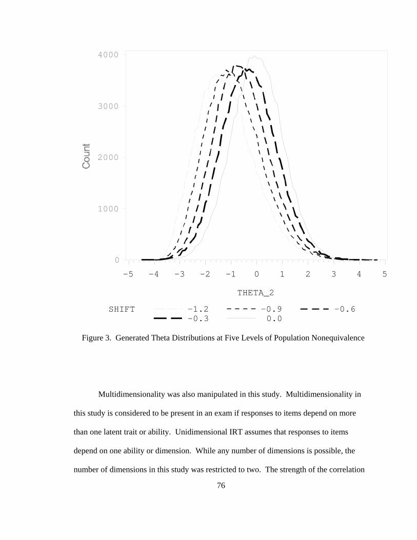
76

Figure 3. Generated Theta Distributions at Five Levels of Population Nonequivalence

Multidimensionality was also manipulated in this study. Multidimensionality in

this study is considered to be present in an exam if responses to items depend on more

than one latent trait or ability. Unidimensional IRT assumes that responses to items

depend on one ability or dimension. While any number of dimensions is possible, the

number of dimensions in this study was restricted to two. The strength of the correlation

SHIFT -1.2 -0.9 -0.6-0.3 0.0

0

1000

2000

3000

4000

THETA_2

-5 -4 -3 -2 -1 0 1 2 3 4 5

77

between the two dimensions was manipulated to model levels of dimensionality. The

levels of dimensionality for Phase One, rθ1θ2 = .90, .70, .50, .40, and .30, were selected

based on information gleaned from Bolt’s (1999) study.

The third and fourth variables I manipulated in Phase One were equivalent item

discriminations and the presence of guessing, respectively. Nonequivalent

discriminations were chosen to be manipulated, to replicate the findings of previous

research conducted with actual test data that showed preequating produced acceptable

precision around the mean of the scale score with forms containing nonequivalent point

biserial correlations with means of .35 and standard deviations of .17 (Du et al., 2002).

Guessing was included in this study because it has repeatedly caused problems for

parameter invariance in prior studies. Most importantly, these variables were

manipulated to determine how tolerant preequating was to the interaction of

multidimensionality, population nonequivalence, equivalent item discriminations, and the

presence of guessing. Despite an extensive literature review, I am not aware of any

previous studies that have investigated these exact interactions under the 1PL model.

A uniform distribution (U) was used to model the a and c parameters (Baker &

AL-Karni, 1991; Kaskowitz & De Ayala, 2001; Kim, 2006; Swaminathan & Gifford,

1986). To manipulate the equivalence of item discriminations, the a parameters were

manipulated at five levels (U(1,1), U(.70, 1.0), U(.50, 1.10), U(.40, 1.20), U(.30, 1.30).

Since item discriminations contribute to test reliability, the simulated a parameters were

manipulated so that the height of the TIFs remained approximately constant. This kept

the test reliability approximately consistent across levels. The target reliability of the

forms was 0.90, which is appropriate for a high stakes test. The levels of the c parameter

78

misspecification scale (U(0,.05, U(0,.10), U(0,.15), U(0,.20), U(0, .25)) were chosen to

cover the range of what is typically seen in three parameter models under four option

multiple choice exams.

Equating Criteria

While there is no consensus on the best measures of equating effectiveness (Kolen

& Brennan, 2004), three commonly employed measures used in equating studies include:

(1) the Root Mean Square Error (RMSE), (2) the Standard Error of Equating (SEE), and

(3) bias of the equated raw scores (Hanson & Beguin, 2002; Pomplun, Omar, & Custer,

2004). These measures represent total equating error, random equating error, and

systematic equating error, respectively. Total error and systematic error were calculated

with the formulas below:

rhhHRMSE yyy /)ˆ()( 2−= ∑ (3.1)

rhhHBIAS yyy /)ˆ()( −= ∑ (3.2)

In calculating equating error, yh is the criterion equated score and yh is the

estimated equated raw score, and r is the number of replications. Negative bias values

indicate that the estimated equated score is less than the criterion. In this study r = 20.

The RMSE and bias were calculated at each raw score point.

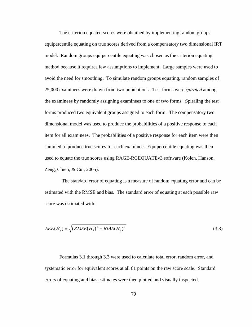
79

The criterion equated scores were obtained by implementing random groups

equipercentile equating on true scores derived from a compensatory two dimensional IRT

model. Random groups equipercentile equating was chosen as the criterion equating

method because it requires few assumptions to implement. Large samples were used to

avoid the need for smoothing. To simulate random groups equating, random samples of

25,000 examinees were drawn from two populations. Test forms were spiraled among

the examinees by randomly assigning examinees to one of two forms. Spiraling the test

forms produced two equivalent groups assigned to each form. The compensatory two

dimensional model was used to produce the probabilities of a positive response to each

item for all examinees. The probabilities of a positive response for each item were then

summed to produce true scores for each examinee. Equipercentile equating was then

used to equate the true scores using RAGE-RGEQUATEv3 software (Kolen, Hanson,

Zeng, Chien, & Cui, 2005).

The standard error of equating is a measure of random equating error and can be

estimated with the RMSE and bias. The standard error of equating at each possible raw

score was estimated with:

22 )()(()( iii HBIASHRMSEHSEE −= (3.3)

Formulas 3.1 through 3.3 were used to calculate total error, random error, and

systematic error for equivalent scores at all 61 points on the raw score scale. Standard

errors of equating and bias estimates were then plotted and visually inspected.

80

Parameter Recovery

Formula 3.1 was used to calculate the total error of the assumed a, estimated b,

and assumed c item parameters. In calculating item parameter error, yh was the

generated item parameter for item γ and yh was the estimated item parameter, and r was

the number of replications.

Phase One Conditions

In Phase One, each variable was manipulated at five levels while all other

variables were kept ideal and constant. Table 3 shows the 17 conditions. Each condition

consisted of a sample size of 500 examinees. A total number of 20 bootstrap samples

were drawn with replacement for each experimental condition. While precedence would

suggest 50 replications are necessary to obtain good SEE estimates with the 3PL model

(Kim & Cohen, 1998; Hanson & Beguin, 2002; Kim, 2006; Li and Lissitz, 2004), I

discovered by experimentation, that only 20 replications were necessary to obtain

adequate precision in the SEE with the Rasch model (Figure 4). Figure 4 shows a

comparison between standard errors of equating estimated with 20 and 50 replications.

These estimates were based on samples of only 100 examinees. These results likely

overstate the difference that would be seen with sample sizes of 500. The added

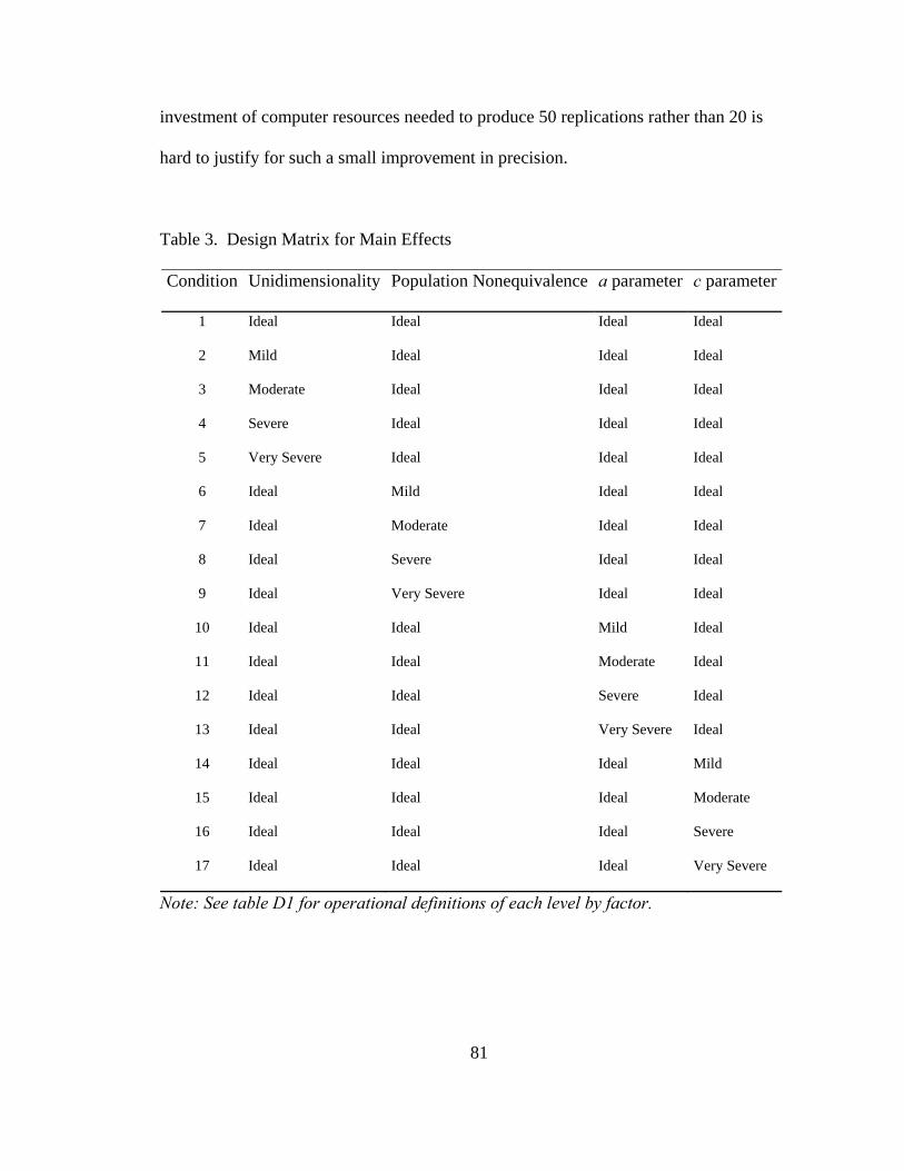
81

investment of computer resources needed to produce 50 replications rather than 20 is

hard to justify for such a small improvement in precision.

Table 3. Design Matrix for Main Effects

Condition Unidimensionality Population Nonequivalence a parameter c parameter

1 Ideal Ideal Ideal Ideal

2 Mild Ideal Ideal Ideal

3 Moderate Ideal Ideal Ideal

4 Severe Ideal Ideal Ideal

5 Very Severe Ideal Ideal Ideal

6 Ideal Mild Ideal Ideal

7 Ideal Moderate Ideal Ideal

8 Ideal Severe Ideal Ideal

9 Ideal Very Severe Ideal Ideal

10 Ideal Ideal Mild Ideal

11 Ideal Ideal Moderate Ideal

12 Ideal Ideal Severe Ideal

13 Ideal Ideal Very Severe Ideal

14 Ideal Ideal Ideal Mild

15 Ideal Ideal Ideal Moderate

16 Ideal Ideal Ideal Severe

17 Ideal Ideal Ideal Very Severe

Note: See table D1 for operational definitions of each level by factor.

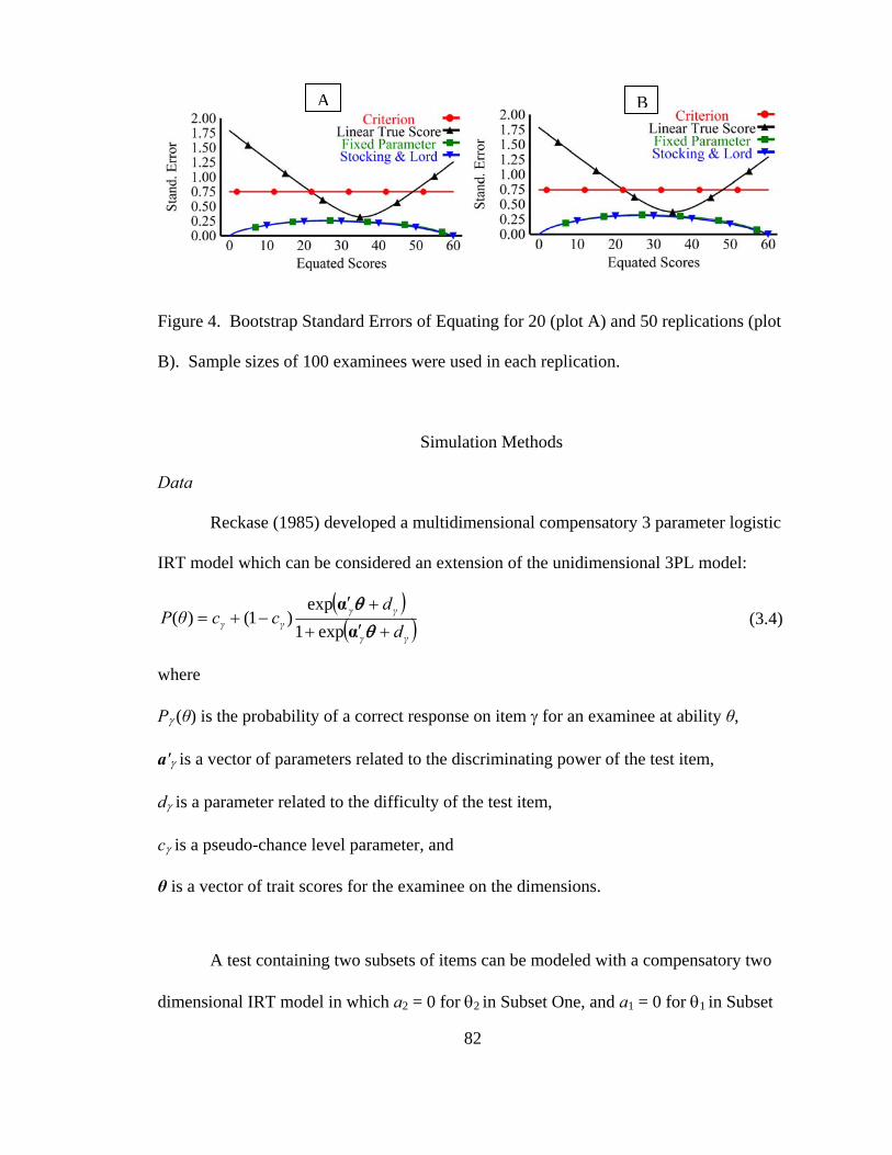
82

Figure 4. Bootstrap Standard Errors of Equating for 20 (plot A) and 50 replications (plot

B). Sample sizes of 100 examinees were used in each replication.

Simulation Methods

Data

Reckase (1985) developed a multidimensional compensatory 3 parameter logistic

IRT model which can be considered an extension of the unidimensional 3PL model:

( )( )γγ

γγγγ d

dccθP

+ ′+

+ ′−+=

θθα

αexp1

exp)1()(

(3.4)

where

Pγ (θ) is the probability of a correct response on item γ for an examinee at ability θ,

a'γ is a vector of parameters related to the discriminating power of the test item,

dγ is a parameter related to the difficulty of the test item,

cγ is a pseudo-chance level parameter, and

θ is a vector of trait scores for the examinee on the dimensions.

A test containing two subsets of items can be modeled with a compensatory two

dimensional IRT model in which a2 = 0 for θ2 in Subset One, and a1 = 0 for θ1 in Subset

A B

83

Two (Reckase, Ackerman, & Carlson, 1988). This is equivalent to using a

unidimensional model to simulate Subset One using θ1, simulating Subset Two using θ2,

and then combining Subset One and Subset Two to form one test. I used the latter of

these two methods to generate response data from a two dimensional compensatory

model.

Items 1 - 30 made up Subset One, and items 31 – 60 made up Subset Two. θj1

was used to simulate Subset One for person j, and θj2 was used for Subset Two and

person j. The correlation of each theta varied according to the condition. For Subset

One, item responses for 100,000 examinees per time period were simulated according to

the 3PL IRT model by sampling abilities from the θ1 distribution and using the IRT item

parameters (Tables B1, B2, and B3 in Appendix B). Item response probabilities were

then computed according to the IRT 3PL model, and in each case, the probability was

compared to a random uniform number. If the response probability was greater than the

random number, the response was coded 1; otherwise the response was coded 0. Item

responses for subset 2 for person j were produced in the same manner by sampling

abilities from the θ2 distribution. Then Subset One and Subset Two were combined to

form a single test. Once item responses were generated for each condition, Bigsteps was

used to estimate item parameters using the FPC method and separate calibration.

Item Linking Simulation Procedures

In order to perform an item parameter recovery study, it was necessary to place all

item parameter estimates on the same scale as the generated item parameters (Yen &

84

Fitzpatrick, 2006). Yen and Fitzpatrick (2006) recommend linking estimated items to the

generated items to ensure that the estimated and generated item parameters are

comparable. Because the modeled data were multidimensional, an extra procedure was

necessary to link the estimated item parameters to the generating item parameters. Doran

and Kingston (1985) devised a five step procedure to place item parameters estimated

under multidimensional conditions onto the scale of the item parameters estimated under

unidimensional conditions. I used a variation of this Doran and Kingston procedure to

place the estimated item parameters from multidimensional tests onto the scale of the

generated item parameters. First, I calibrated Subset One and linked these item

parameter estimates to the scale of the generated items. Second, I calibrated Subset Two

and linked these item parameter estimates to the scale of the generated items. Finally, I

combined the linked item parameter estimates from Subset One and Subset Two to form

a complete set. Once the estimated item parameters were placed on the generated scale, I

linked all subsequent pilot items from each form in the usual manner, ignoring the

multidimensional nature of the data.

Figure 5 displays the linking plan devised for Phase One. This bank consists of

100 items. Form A in time period one consists of 60 operational items, and 20 pilot

items. According to this plan, the 20 pilot items from time period one are treated as

operational items in form B during time period two.

85

Figure 5. Linking Plan and Assignment of Items to Forms in Phase One

Phase Two

Phase two extended Phase One in a number of important ways. Firstly, in Phase

Two, I examined the interaction effects of violations of model assumptions. Secondly,

because the overarching purpose of this study was to define the limits of preequating and

since preequating was generally robust to violations of assumptions in Phase One, I

elected to lower the sample size from 500 to 100 in an effort to force preequating to

produce larger standard errors of equating. If preequating worked adequately with small

samples as small as 100, then the utility of the method would increase, especially for

smaller testing programs. Thirdly, to determine if equating precision and accuracy

deteriorated across item calibrations (research question 5d and hypothesis 5), I examined

equating error across five forms rather than two.

Item Bank of 100 items

Form A

Form B

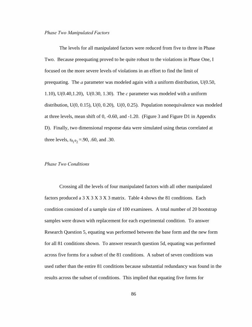
86

Phase Two Manipulated Factors

The levels for all manipulated factors were reduced from five to three in Phase

Two. Because preequating proved to be quite robust to the violations in Phase One, I

focused on the more severe levels of violations in an effort to find the limit of

preequating. The a parameter was modeled again with a uniform distribution, U(0.50,

1.10), U(0.40,1.20), U(0.30, 1.30). The c parameter was modeled with a uniform

distribution, U(0, 0.15), U(0, 0.20), U(0, 0.25). Population nonequivalence was modeled

at three levels, mean shift of 0, -0.60, and -1.20. (Figure 3 and Figure D1 in Appendix

D). Finally, two dimensional response data were simulated using thetas correlated at

three levels, rθ1θ2 =.90, .60, and .30.

Phase Two Conditions

Crossing all the levels of four manipulated factors with all other manipulated

factors produced a 3 X 3 X 3 X 3 matrix. Table 4 shows the 81 conditions. Each

condition consisted of a sample size of 100 examinees. A total number of 20 bootstrap

samples were drawn with replacement for each experimental condition. To answer

Research Question 5, equating was performed between the base form and the new form

for all 81 conditions shown. To answer research question 5d, equating was performed

across five forms for a subset of the 81 conditions. A subset of seven conditions was

used rather than the entire 81 conditions because substantial redundancy was found in the

results across the subset of conditions. This implied that equating five forms for

87

additional conditions would produce little new knowledge. Table 4 provides the number

of forms equated per condition.

To summarize and describe the interaction effects of multidimensionality,

population nonequivalence, nonequivalent a parameters, and guessing on equating error,

analysis of variance was conducted. Global measures of equating bias and SEE were

used to summarize error across all raw score points. Even though the SEE and bias

varied across the score continuum, the pattern of the variation was consistent across

conditions. The pattern of preequating bias tended to reach its maximum value at lower

raw scores and diminished across the rest of the score continuum. The pattern of the

preequating SEE tended to reach its maximum near the mean of the score distribution and

its minimum toward the scale extremes. Considering the consistency of the patterns

shown in the preequating bias and SEE, it seemed reasonable to use means to summarize

the equating error across the scale. Absolute differences between the criterion score and

the mean equated score from 20 replications were averaged across 61 raw score points to

calculate a global measure of equating bias. Absolute values were used because the

direction of bias varied across the raw score scale. The SEE was also averaged across 61

raw score points to produce the mean standard error of equating (MSEE). The mean

absolute bias of equating and the MSEE were then subjected to ANOVA to obtain effect

size measures of the main and interaction effects of all conditions in Phase Two.

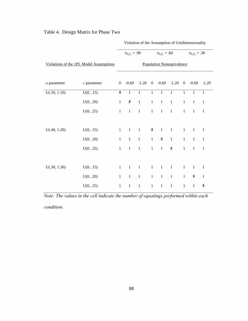
88

Table 4. Design Matrix for Phase Two

Violation of the Assumption of Unidimensionality

rθ1θ2 = .90 rθ1θ2

= .60 rθ1θ2 = .30

Violations of the 1PL Model Assumptions Population Nonequivalence

a parameter c parameter 0 -0.60 -1.20 0 -0.60 -1.20 0 -0.60 -1.20

U(.50, 1.10) U(0, .15) 5 1 1 1 1 1 1 1 1

U(0, .20) 1 5 1 1 1 1 1 1 1

U(0, .25) 1 1 1 1 1 1 1 1 1

U(.40, 1.20) U(0, .15) 1 1 1 5 1 1 1 1 1

U(0, .20) 1 1 1 1 5 1 1 1 1

U(0, .25) 1 1 1 1 1 5 1 1 1

U(.30, 1.30) U(0, .15) 1 1 1 1 1 1 1 1 1

U(0, .20) 1 1 1 1 1 1 1 5 1

U(0, .25) 1 1 1 1 1 1 1 1 5

Note: The values in the cell indicate the number of equatings performed within each

condition.

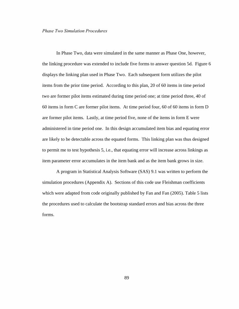
89

Phase Two Simulation Procedures

In Phase Two, data were simulated in the same manner as Phase One, however,

the linking procedure was extended to include five forms to answer question 5d. Figure 6

displays the linking plan used in Phase Two. Each subsequent form utilizes the pilot

items from the prior time period. According to this plan, 20 of 60 items in time period

two are former pilot items estimated during time period one; at time period three, 40 of

60 items in form C are former pilot items. At time period four, 60 of 60 items in form D

are former pilot items. Lastly, at time period five, none of the items in form E were

administered in time period one. In this design accumulated item bias and equating error

are likely to be detectable across the equated forms. This linking plan was thus designed

to permit me to test hypothesis 5, i.e., that equating error will increase across linkings as

item parameter error accumulates in the item bank and as the item bank grows in size.

A program in Statistical Analysis Software (SAS) 9.1 was written to perform the

simulation procedures (Appendix A). Sections of this code use Fleishman coefficients

which were adapted from code originally published by Fan and Fan (2005). Table 5 lists

the procedures used to calculate the bootstrap standard errors and bias across the three

forms.

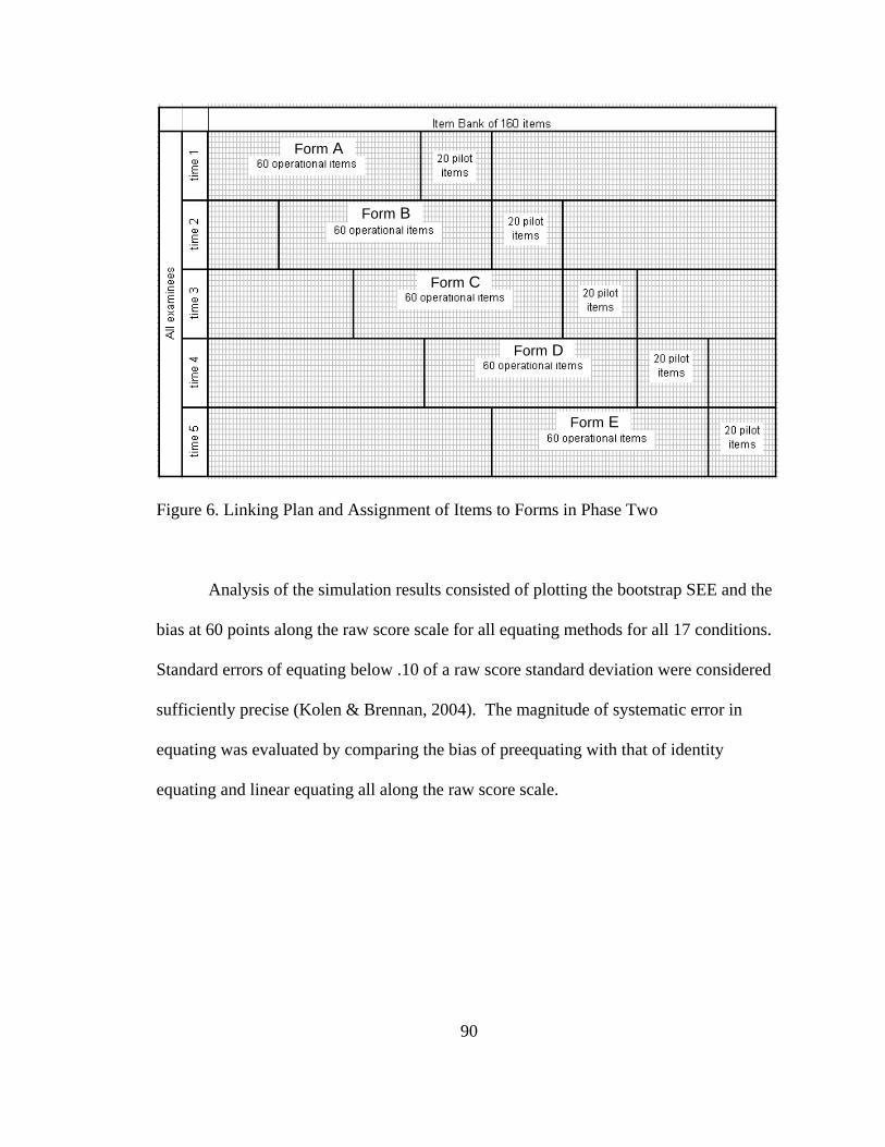
90

Figure 6. Linking Plan and Assignment of Items to Forms in Phase Two

Analysis of the simulation results consisted of plotting the bootstrap SEE and the

bias at 60 points along the raw score scale for all equating methods for all 17 conditions.

Standard errors of equating below .10 of a raw score standard deviation were considered

sufficiently precise (Kolen & Brennan, 2004). The magnitude of systematic error in

equating was evaluated by comparing the bias of preequating with that of identity

equating and linear equating all along the raw score scale.

Form A

Form B

Form C

Form D

Form E

91

Table 5. Steps to Calculating Bootstrap Standard Error and Bias Across Specified

Number of Forms

Order Step Set up simulation 1 Generate 2 populations of 100,000 examinees each 2 Randomly sample 25,000 examinees from population 1 3 Obtain the base form

Create criterion conversion table 4 Obtain the new form 5 Randomly sample 25,000 examinees from population 2 6

Randomly assign examinees from step 2 and 5 to both forms, producing equivalent Groups

7

Calculate true scores for base and new form using generated parameters and 3PL compensatory 2D model

8 Equate true scores from base and new form using random groups equipercentile equating

Administer exam with pilot items 9 Randomly sample examinees from population 1

10 Create response strings using generated item parameters from base form and thetas from sample

Calibrate operational items 11 Estimate operational item parameters for base form using Bigsteps 12 Calibrate operational items in subtest 1 to generated item scale using SCSL 13 Calibrate operational items in subtest 2 to generated item scale using SCSL

Calibrate pilot items and preequated 14 Calibrate pilot items with the Rasch model using FPC and then SCSL and add pilot items to pool 15 Preequate new form to base form

Administer new form with pilot items 16 Randomly sample examinees from population 2 17 Create response strings using generated item parameters from new form and thetas from sample 18 Perform Levine true score equating (chain to original form if necessary) 19

Calibrate pilot items from new form using FPC and then SCSL and add pilot items to pool

Repeat procedures

21

Repeat steps 4 through 8 and steps 4 through 19 for specified number of forms within replication 1

22

Repeat steps 9 - 21 for 20 replications to obtain bias of equating and SEE for specified Forms

92

CHAPTER FOUR

RESULTS

Phase One

Preequating was first performed under ideal conditions to define a baseline for

comparing the performance of Rasch preequating under conditions of violated

assumptions. Figure 7 displays summary graphs for an ideal condition. Plot 1 shows

four equivalent, normally distributed theta distributions used for generating response

data. Plot 2 shows a scree plot illustrating the unidimensional nature of the data. Plots 3

through 5 display the RMSE of the assumed a, estimated b, and assumed c item

parameters. These plots display the RMSE of parameters associated with each

calibration method (FPC and SCSL). Under this ideal condition the item parameters

remain uniformly flat and close to zero for all assumed and estimated parameters. Plot 6

shows the true score distributions derived from the generated theta and item parameters.

These true score distributions were used in defining the criterion equating function via

random groups equipercentile equating. The difference between these two distributions

is caused by form differences, since the two groups for each form attained equivalence

via random assignment. Plot 7 and 8 are Test Characteristic Curves derived from item

parameter estimates obtained from the FPC method and the SCSL methods, respectively.

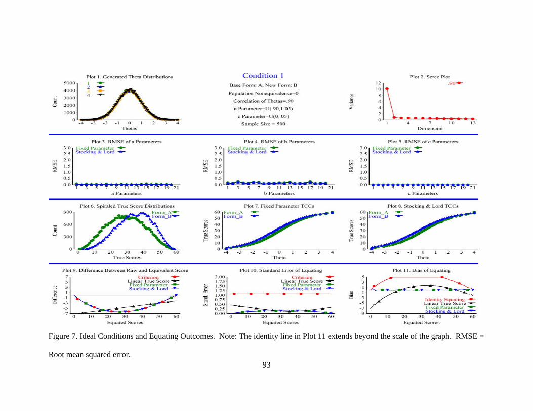
93

Figure 7. Ideal Conditions and Equating Outcomes. Note: The identity line in Plot 11 extends beyond the scale of the graph. RMSE =

Root mean squared error.

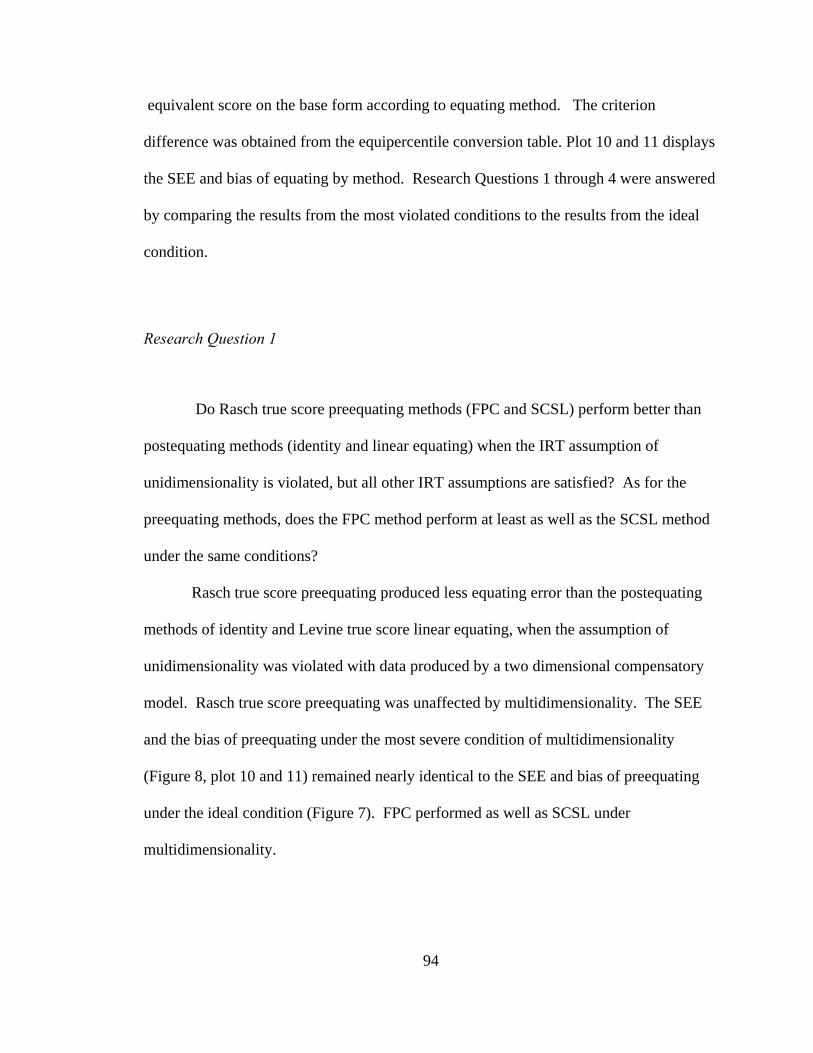
94

equivalent score on the base form according to equating method. The criterion

difference was obtained from the equipercentile conversion table. Plot 10 and 11 displays

the SEE and bias of equating by method. Research Questions 1 through 4 were answered

by comparing the results from the most violated conditions to the results from the ideal

condition.

Research Question 1

Do Rasch true score preequating methods (FPC and SCSL) perform better than





Rasch true score preequating produced less equating error than the postequating

methods of identity and Levine true score linear equating, when the assumption of

unidimensionality was violated with data produced by a two dimensional compensatory

model. Rasch true score preequating was unaffected by multidimensionality. The SEE

and the bias of preequating under the most severe condition of multidimensionality

(Figure 8, plot 10 and 11) remained nearly identical to the SEE and bias of preequating

under the ideal condition (Figure 7). FPC performed as well as SCSL under

multidimensionality.

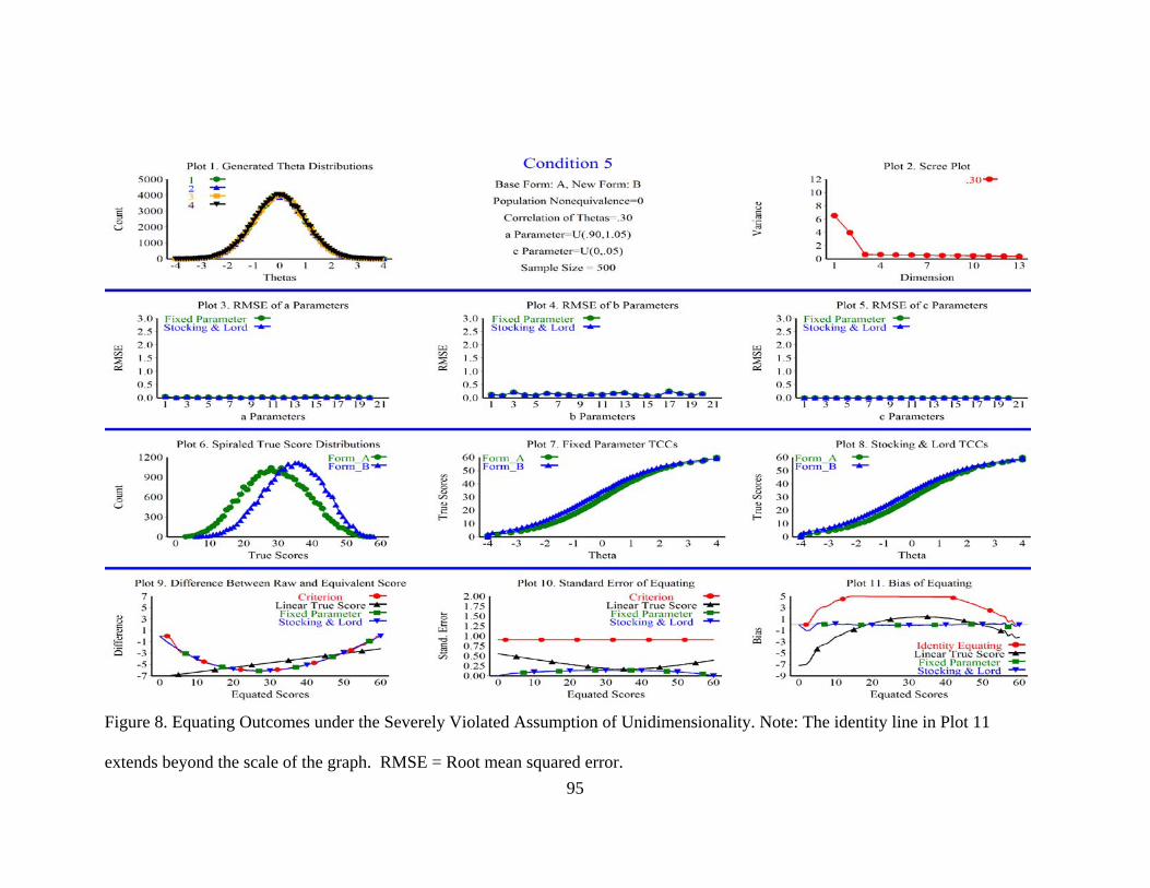
95

Figure 8. Equating Outcomes under the Severely Violated Assumption of Unidimensionality. Note: The identity line in Plot 11

extends beyond the scale of the graph. RMSE = Root mean squared error.

96

Research Question 2


postequating methods (identity and Linear equating) when populations are




methods of identity and Levine true score linear equating when populations were

nonequivalent and all other IRT assumptions were satisfied. The SEE and the bias of

preequating under the most severe condition of nonequivalence (Figure 9, plot 10 and 11)

remained nearly identical to the SEE and bias of preequating under the ideal condition

(Figure 7). The FPC method performed as well as the SCSL under population

nonequivalence.

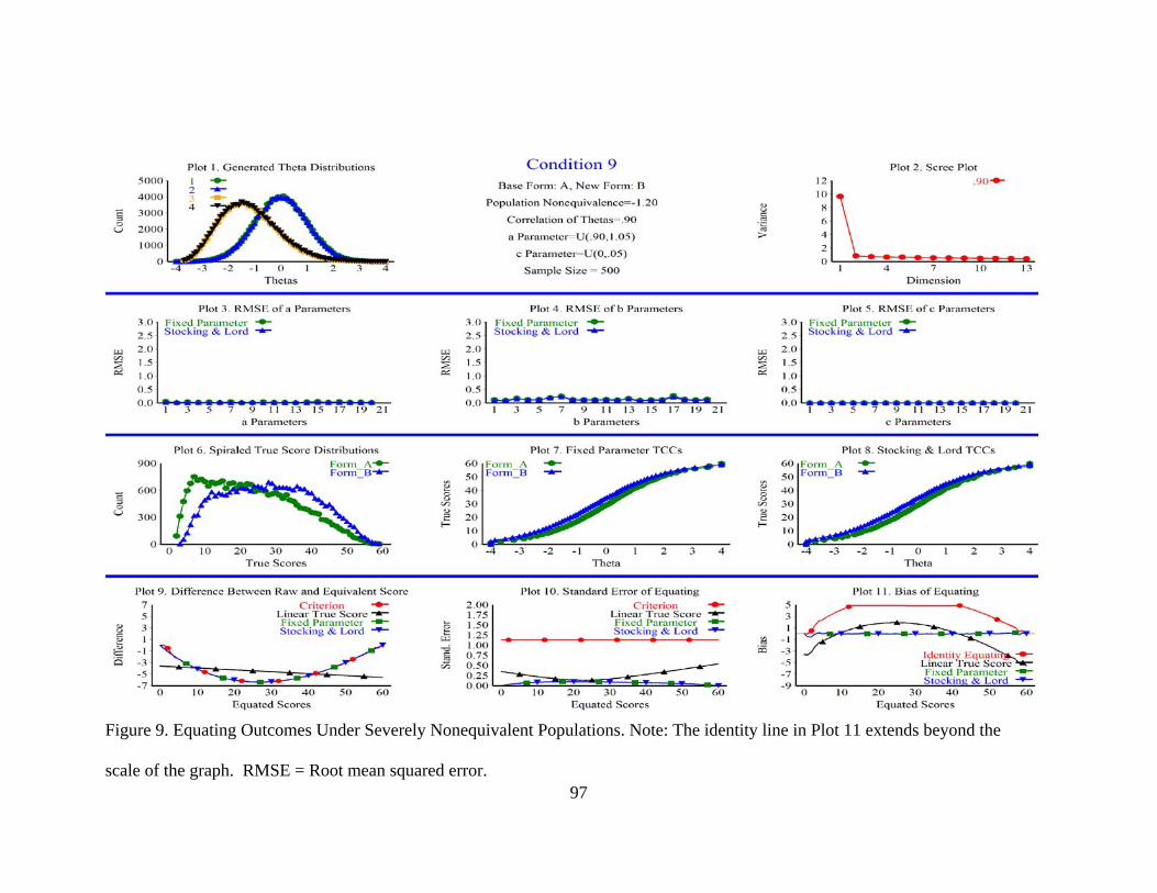
97

Figure 9. Equating Outcomes Under Severely Nonequivalent Populations. Note: The identity line in Plot 11 extends beyond the

scale of the graph. RMSE = Root mean squared error.

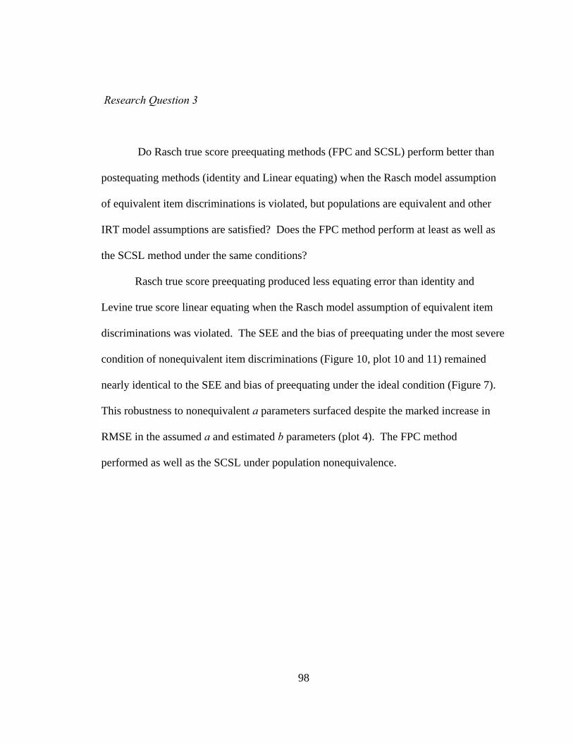
98

Research Question 3






Rasch true score preequating produced less equating error than identity and

Levine true score linear equating when the Rasch model assumption of equivalent item

discriminations was violated. The SEE and the bias of preequating under the most severe

condition of nonequivalent item discriminations (Figure 10, plot 10 and 11) remained

nearly identical to the SEE and bias of preequating under the ideal condition (Figure 7).

This robustness to nonequivalent a parameters surfaced despite the marked increase in

RMSE in the assumed a and estimated b parameters (plot 4). The FPC method

performed as well as the SCSL under population nonequivalence.

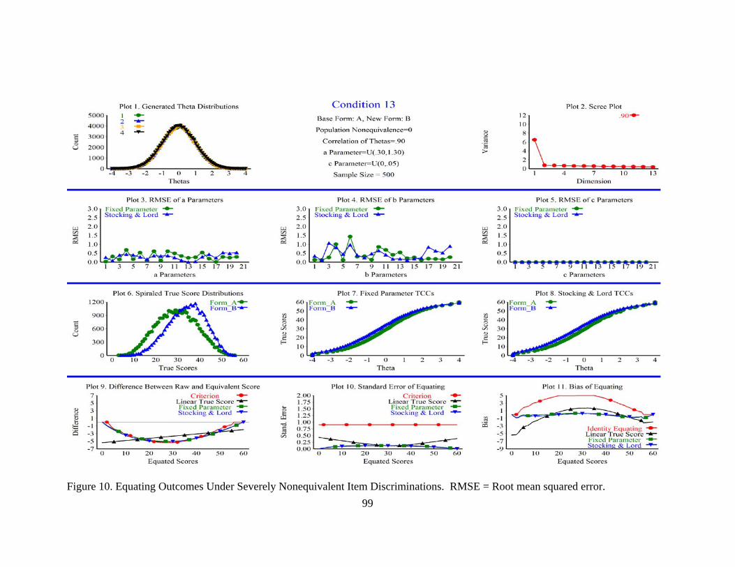
99

Figure 10. Equating Outcomes Under Severely Nonequivalent Item Discriminations. RMSE = Root mean squared error.

100

Research Question 4



of no guessing is violated, but populations are equivalent and other IRT model

assumptions are satisfied? Does the FPC method perform at least as well as the SCSL

method under the same conditions?


methods of identity and Levine true score linear equating when the Rasch model

assumption of no guessing was violated, but populations were equivalent and other

IRT model assumptions were satisfied. The SEE of preequating under the most severe

condition of guessing (Figure 11, plot 10 and 11) remained nearly identical to the SEE of

preequating under the ideal condition (Figure 7). Bias increased under the severe

condition of guessing. Equating bias was maximum at the lower end of the score scale

(plot 11), when the no guessing assumption was severely violated (plot 5). The FPC

method performed as well as the SCSL under population nonequivalence.

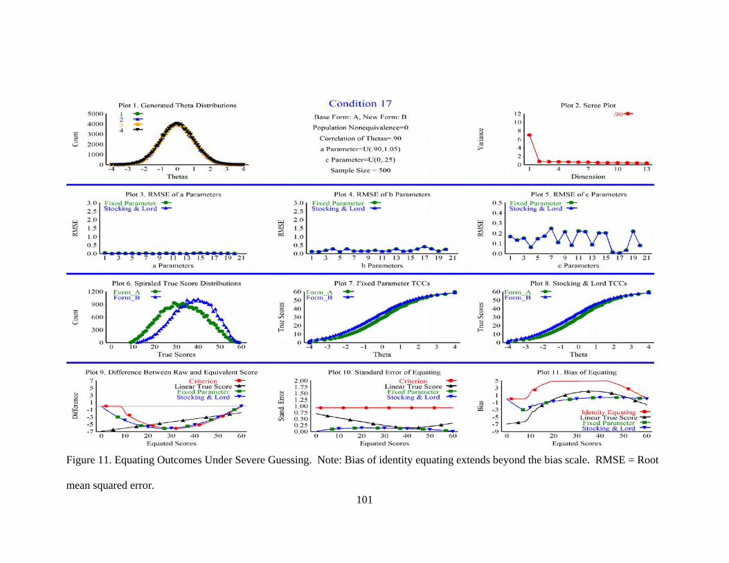
101

Figure 11. Equating Outcomes Under Severe Guessing. Note: Bias of identity equating extends beyond the bias scale. RMSE = Root

mean squared error.

102

Phase Two

Research Question 5a

What are the interaction effects of multidimensionality, population

nonequivalence, nonequivalent item discriminations (a parameters), and guessing (c

parameters) on random and systematic equating error?

Table 6 displays the mean absolute bias for all conditions. The mean absolute

bias ranged from 0.51 to 1.48. The absolute bias was least when the a parameter ranged

from .40 to 1.20 and the c parameter ranged from 0 to .15. The absolute bias was greatest

when the a parameter ranged from .30 to 1.30, the c parameter ranged from 0 to .25, and

populations nonequivalence was -1.20. Table 7 presents η2 effect sizes for each main and

interaction effect. The interaction effect of nonequivalent a parameters and guessing

explained 67 percent of the variance in the bias of the SCSL method, and 71 percent of

the variance in the bias of the FPC method. The main effect of guessing explained 18

percent of the variance in the bias of the SCSL method, and 18 percent of the variance in

the bias of the FPC method. The main effect of nonequivalent a parameters explained ten

percent of the variance in the bias of the SCSL method, and five percent of the variance

in the bias of the FPC method. None of the other factors or interactions had meaningful

effects on the bias of preequating.

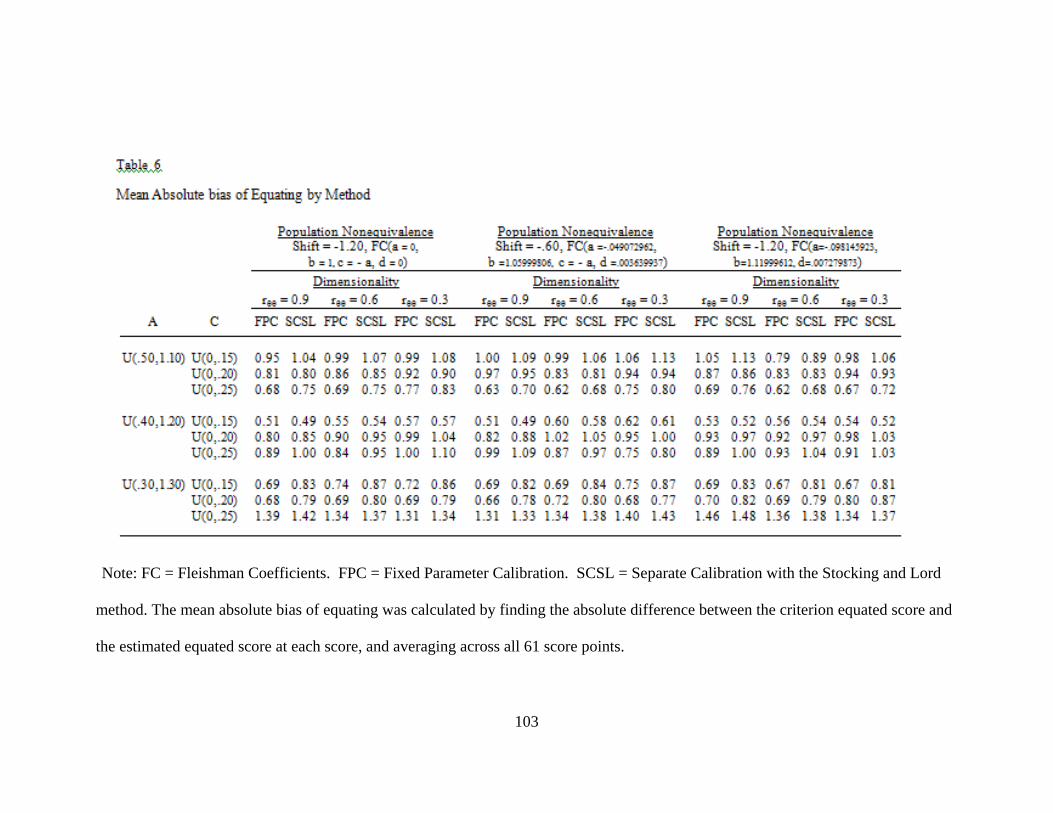
103

Note: FC = Fleishman Coefficients. FPC = Fixed Parameter Calibration. SCSL = Separate Calibration with the Stocking and Lord

method. The mean absolute bias of equating was calculated by finding the absolute difference between the criterion equated score and

the estimated equated score at each score, and averaging across all 61 score points.

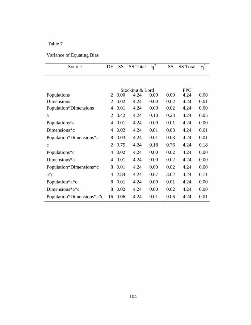
104

Table 7

Variance of Equating Bias

Source DF SS SS Total η2 SS SS Total η2

Stocking & Lord

FPC Populations 2 0.00 4.24 0.00 0.00 4.24 0.00Dimensions 2 0.02 4.24 0.00 0.02 4.24 0.01Population*Dimensions 4 0.01 4.24 0.00 0.02 4.24 0.00a 2 0.42 4.24 0.10 0.23 4.24 0.05Populations*a 4 0.01 4.24 0.00 0.01 4.24 0.00Dimensions*c 4 0.02 4.24 0.01 0.03 4.24 0.01Population*Dimensions*a 8 0.03 4.24 0.01 0.03 4.24 0.01c 2 0.75 4.24 0.18 0.76 4.24 0.18Populations*c 4 0.02 4.24 0.00 0.02 4.24 0.00Dimensions*a 4 0.01 4.24 0.00 0.02 4.24 0.00Population*Dimensions*c 8 0.01 4.24 0.00 0.02 4.24 0.00a*c 4 2.84 4.24 0.67 3.02 4.24 0.71Population*a*c 8 0.01 4.24 0.00 0.01 4.24 0.00Dimensions*a*c 8 0.02 4.24 0.00 0.02 4.24 0.00Population*Dimensions*a*c 16 0.06 4.24 0.01 0.06 4.24 0.01

105

Table 8 displays the MSEE for all Phase Two conditions. The MSEE ranged

from 0.14 to 0.36. Table 9 presents η2 effect sizes for each condition. The interaction of

population nonequivalence, multidimensionality, nonequivalent item discriminations, and

guessing explained the largest portion of the variance at 17 percent. While the

interactions of the violated assumptions were present, there was not a substantial amount

of total variance to explain. Violations of model assumptions had no meaningful effect

on the variance of the MSEE. These results underscore the fact that the SEE for Rasch

preequating is primarily a function of sample size.

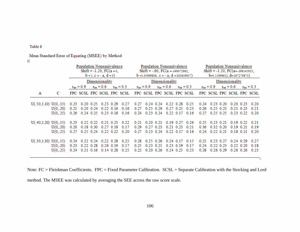
106

Note: FC = Fleishman Coefficients. FPC = Fixed Parameter Calibration. SCSL = Separate Calibration with the Stocking and Lord

method. The MSEE was calculated by averaging the SEE across the raw score scale.

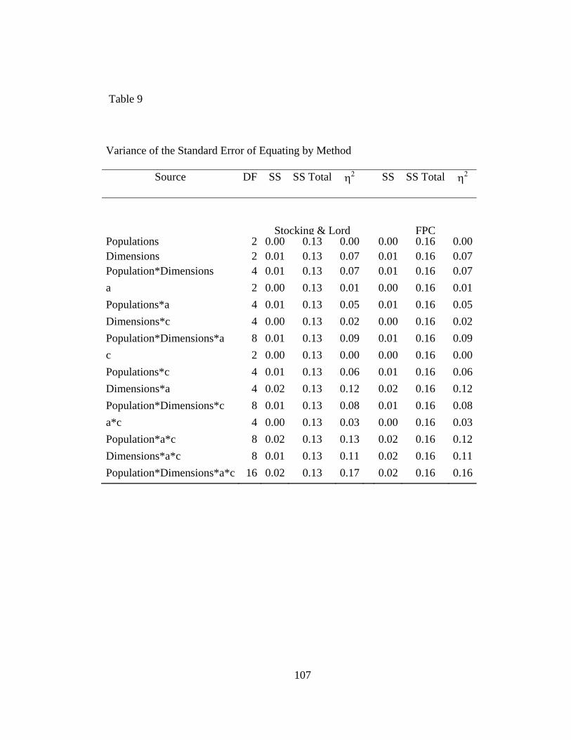
107

Table 9

Variance of the Standard Error of Equating by Method

Source DF SS SS Total η2 SS SS Total η2

Stocking & Lord

FPC Populations 2 0.00 0.13 0.00 0.00 0.16 0.00Dimensions 2 0.01 0.13 0.07 0.01 0.16 0.07Population*Dimensions 4 0.01 0.13 0.07 0.01 0.16 0.07a 2 0.00 0.13 0.01 0.00 0.16 0.01Populations*a 4 0.01 0.13 0.05 0.01 0.16 0.05Dimensions*c 4 0.00 0.13 0.02 0.00 0.16 0.02Population*Dimensions*a 8 0.01 0.13 0.09 0.01 0.16 0.09c 2 0.00 0.13 0.00 0.00 0.16 0.00Populations*c 4 0.01 0.13 0.06 0.01 0.16 0.06Dimensions*a 4 0.02 0.13 0.12 0.02 0.16 0.12Population*Dimensions*c 8 0.01 0.13 0.08 0.01 0.16 0.08a*c 4 0.00 0.13 0.03 0.00 0.16 0.03Population*a*c 8 0.02 0.13 0.13 0.02 0.16 0.12Dimensions*a*c 8 0.01 0.13 0.11 0.02 0.16 0.11Population*Dimensions*a*c 16 0.02 0.13 0.17 0.02 0.16 0.16

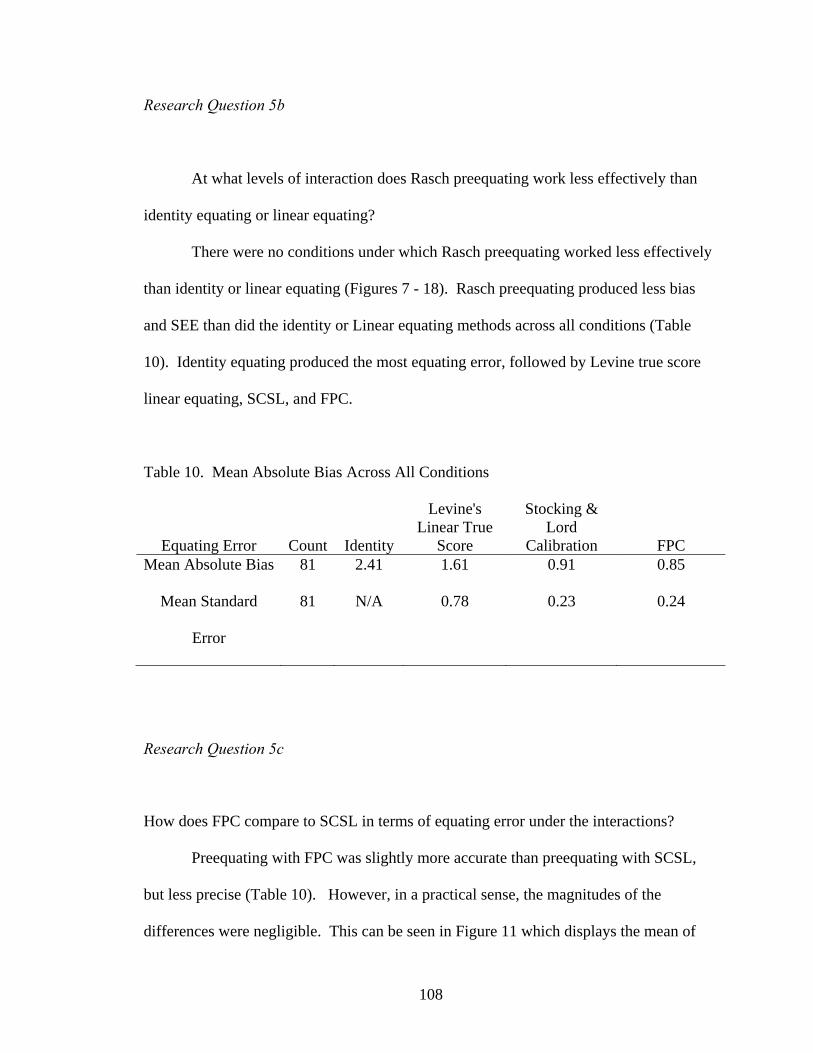
108

Research Question 5b

At what levels of interaction does Rasch preequating work less effectively than

identity equating or linear equating?

There were no conditions under which Rasch preequating worked less effectively

than identity or linear equating (Figures 7 - 18). Rasch preequating produced less bias

and SEE than did the identity or Linear equating methods across all conditions (Table

10). Identity equating produced the most equating error, followed by Levine true score

linear equating, SCSL, and FPC.

Table 10. Mean Absolute Bias Across All Conditions

Equating Error Count Identity

Levine's Linear True

Score

Stocking & Lord

Calibration FPC Mean Absolute Bias 81 2.41 1.61 0.91 0.85

Mean Standard

Error

81 N/A 0.78 0.23 0.24

Research Question 5c

How does FPC compare to SCSL in terms of equating error under the interactions?

Preequating with FPC was slightly more accurate than preequating with SCSL,

but less precise (Table 10). However, in a practical sense, the magnitudes of the

differences were negligible. This can be seen in Figure 11 which displays the mean of

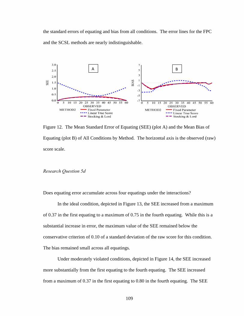
109

the standard errors of equating and bias from all conditions. The error lines for the FPC

and the SCSL methods are nearly indistinguishable.

Figure 12. The Mean Standard Error of Equating (SEE) (plot A) and the Mean Bias of

Equating (plot B) of All Conditions by Method. The horizontal axis is the observed (raw)

score scale.

Research Question 5d

Does equating error accumulate across four equatings under the interactions?

In the ideal condition, depicted in Figure 13, the SEE increased from a maximum

of 0.37 in the first equating to a maximum of 0.75 in the fourth equating. While this is a

substantial increase in error, the maximum value of the SEE remained below the

conservative criterion of 0.10 of a standard deviation of the raw score for this condition.

The bias remained small across all equatings.

Under moderately violated conditions, depicted in Figure 14, the SEE increased

more substantially from the first equating to the fourth equating. The SEE increased

from a maximum of 0.37 in the first equating to 0.80 in the fourth equating. The SEE

A B

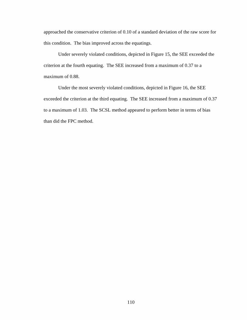
110

approached the conservative criterion of 0.10 of a standard deviation of the raw score for

this condition. The bias improved across the equatings.

Under severely violated conditions, depicted in Figure 15, the SEE exceeded the

criterion at the fourth equating. The SEE increased from a maximum of 0.37 to a

maximum of 0.88.

Under the most severely violated conditions, depicted in Figure 16, the SEE

exceeded the criterion at the third equating. The SEE increased from a maximum of 0.37

to a maximum of 1.03. The SCSL method appeared to perform better in terms of bias

than did the FPC method.

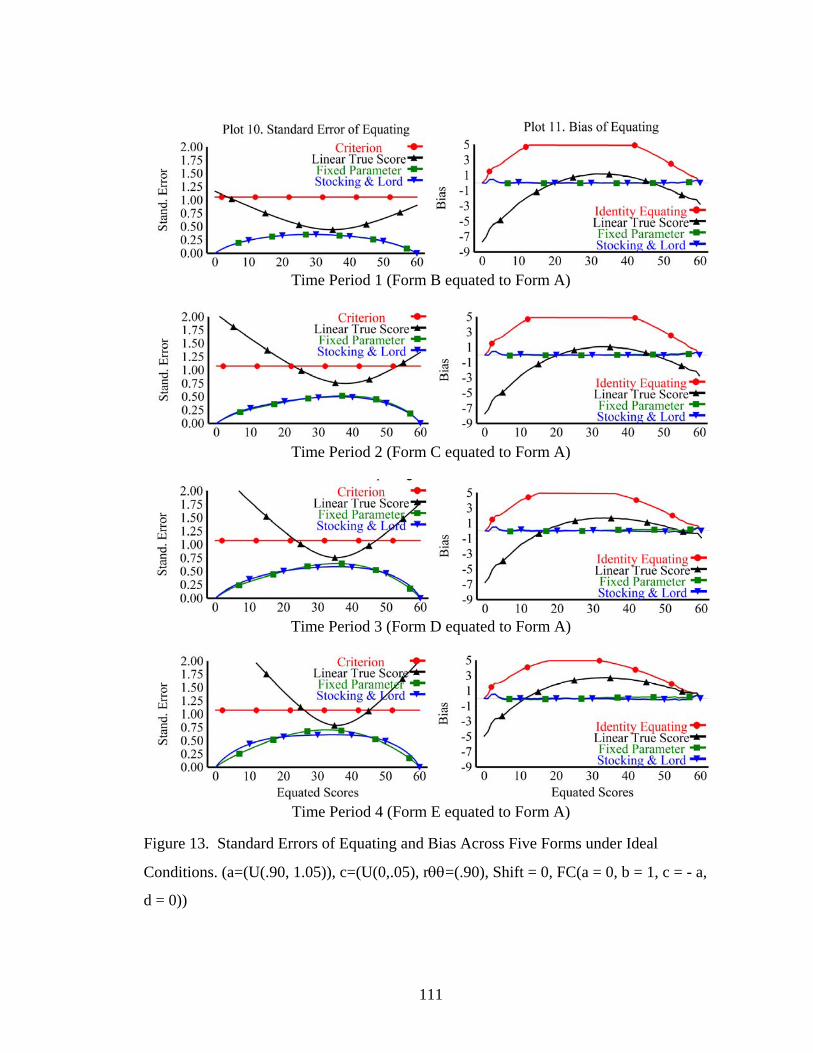
111

Time Period 1 (Form B equated to Form A)

Time Period 2 (Form C equated to Form A)

Time Period 3 (Form D equated to Form A)

Time Period 4 (Form E equated to Form A)

Figure 13. Standard Errors of Equating and Bias Across Five Forms under Ideal

Conditions. (a=(U(.90, 1.05)), c=(U(0,.05), rθθ=(.90), Shift = 0, FC(a = 0, b = 1, c = - a,

d = 0))

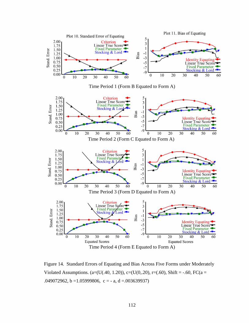
112

Time Period 1 (Form B Equated to Form A)

Time Period 2 (Form C Equated to Form A)

Time Period 3 (Form D Equated to Form A)

Time Period 4 (Form E Equated to Form A)

Figure 14. Standard Errors of Equating and Bias Across Five Forms under Moderately

Violated Assumptions. (a=(U(.40, 1.20)), c=(U(0,.20), r=(.60), Shift = -.60, FC(a =

.049072962, b =1.05999806, c = - a, d =.003639937)

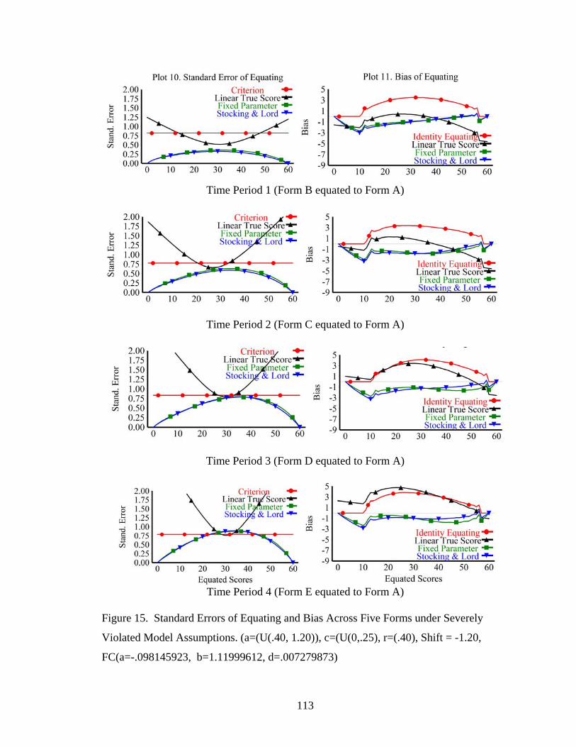
113

Time Period 1 (Form B equated to Form A)

Time Period 2 (Form C equated to Form A)

Time Period 3 (Form D equated to Form A)

Time Period 4 (Form E equated to Form A)

Figure 15. Standard Errors of Equating and Bias Across Five Forms under Severely

Violated Model Assumptions. (a=(U(.40, 1.20)), c=(U(0,.25), r=(.40), Shift = -1.20,

FC(a=-.098145923, b=1.11999612, d=.007279873)

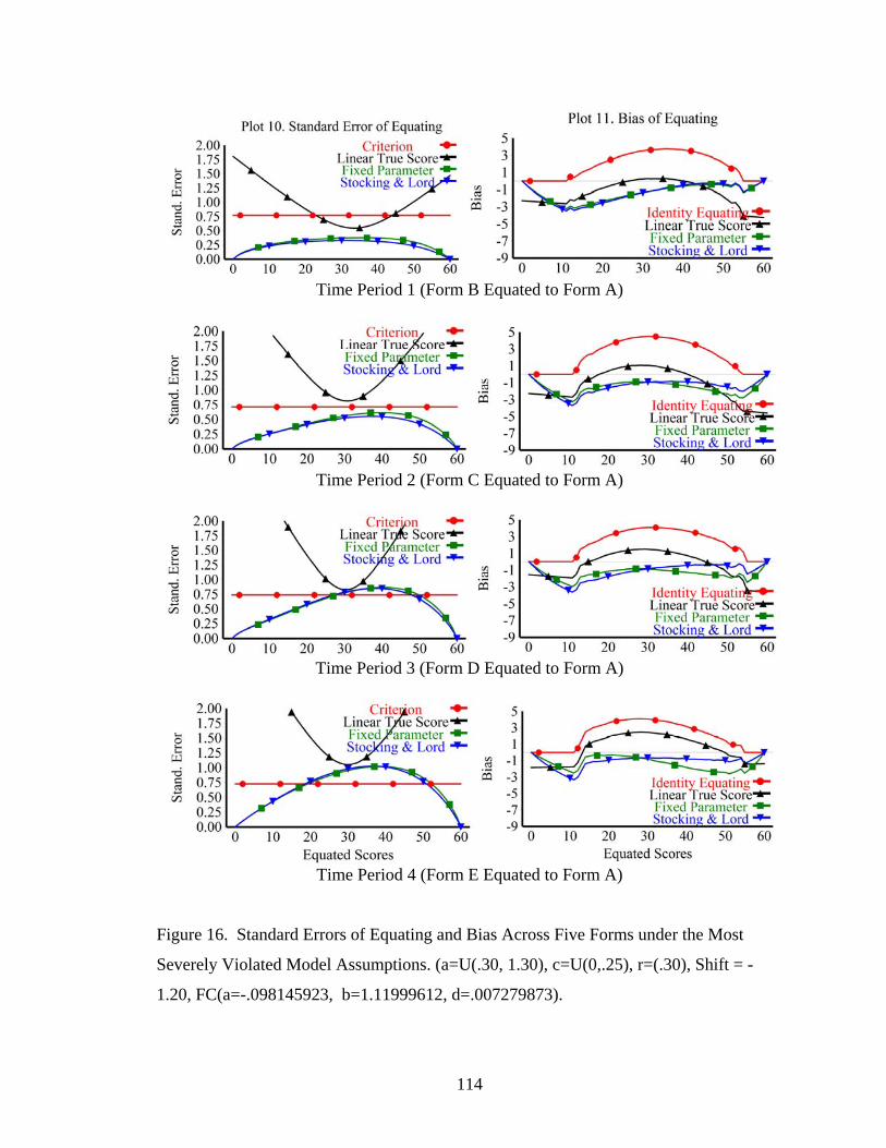
114

Time Period 1 (Form B Equated to Form A)

Time Period 2 (Form C Equated to Form A)

Time Period 3 (Form D Equated to Form A)

Time Period 4 (Form E Equated to Form A)

Figure 16. Standard Errors of Equating and Bias Across Five Forms under the Most

Severely Violated Model Assumptions. (a=U(.30, 1.30), c=U(0,.25), r=(.30), Shift = -

1.20, FC(a=-.098145923, b=1.11999612, d=.007279873).

115

CHAPTER FIVE

DISCUSSION

This chapter presents the substantive conclusions and implications of the study.

First, the results for Phase One and Phase Two are summarized, followed by a discussion

of the four hypotheses presented in the methods section. An explanation is offered for

the cause of preequating’s sensitivity to violations of the no guessing assumption.

Results from an additional condition are then presented that provide support for this

explanation. Implications of the results of this study to classification consistency and

accuracy are discussed. The limitations of the study and suggestions for future research

are then presented.

Phase One

In Phase One, simulation results provide evidence that preequating was robust to

multidimensionality, population nonequivalence, and nonequivalent item discriminations.

The finding that Rasch true score equating is robust to violations of the assumption of

unidimensionality is consistent with studies previously conducted with the 3PL model

(Bogan & Yen, 1983; Camili, Wang, & Fesq, 1995; Cook Dorans, Eignor, & Petersen,

1985; Dorans & Kingston, 1985; Wang, 1985; Yen, 1984; Smith, 1996). However, these

findings do contradict the studies on preequating under the 3PL model that concluded

116

preequating was not robust to multidimensionality (Eignor, 1985; Kolen & Harris, 1990;

Hendrickson & Kolen, 1999). Given the many types of multidimensionality that can be

present, perhaps the robustness of IRT true score equating depends on the type of

multidimensionality. This study provides evidence that Rasch true score equating is

robust to at least one type of multidimensionality: a 2D compensatory model with a

simple structure. The likely cause for this result is the fact that the JMLE procedure

targets a composite theta (Reckase, Ackerman, & Carlson, 1988). Provided that the test

forms are produced consistently according to a blueprint, the same composite measure is

targeted during parameter estimation and equating. This produces consistent and

accurate equating.

Sample sizes of 500 examinees produced very small SEE. The SEE for all

conditions remained well below the conservative criterion of 0.10 standard deviations of

the raw score. In fact the SEE remained below 0.25 of a raw score point across all

conditions. The SEE for preequating remained smaller than linear equating across all

conditions. This outcome was consistent with Kolen and Brennan’s recommendation to

use a sample of 400 examinees for Rasch true score equating (2004).

The bias of preequating remained less than Levine’s true score linear equating

method and less than the identity equating for all conditions. This result that an IRT true

score preequating method produced less equating error than linear equating is consistent

with earlier findings (Bolt, 1995; Kolen & Brennan, 2004).

The accuracy of difficulty parameter estimates in this study were negatively

affected by the nonequivalent a parameters, however, the error in the assumed a and

estimated b parameters had little effect on preequating. Preequating bias reached its

117

maximum at the low end of the score scale when guessing was most severe. These

results were consistent with Du, Lipkins, and Jones’s equating study (2002).

The finding that Rasch true score preequating was not robust to violations of the

assumption of no guessing was consistent with earlier studies that suggested that the

Rasch model does not perform well under guessing (Slinde & Linn, 1978; Loyd &

Hoover, 1981; Skaggs & Lissetz, 1986).

Phase Two

In comparison to identity equating and Levine’s true score equating, Rasch

preequating performed well under the interaction effects of violated assumptions.

However, the magnitude of equating bias in some conditions would be unacceptably

large for some testing applications. The fact that a substantial interaction between

nonequivalent item discriminations and guessing was found in this study, may help

explain the contradictory results of some past studies that have examined the feasibility

of Rasch true score equating. The results of this study suggest that Rasch true score

equating is tolerant of low levels of guessing; however, if low levels of guessing interact

with moderate levels of nonequivalent item discriminations, substantial bias can appear.

It is very likely that when highly and positively skewed ability distributions

coincide with guessing or with nonequivalent discriminations and guessing, then equating

bias at the low end of the score scale would coincide with the large proportion of low

scoring examinees. It can be inferred that this condition would represent the worst case

scenario for Rasch preequating, in which a large proportion of examinees obtain scores in

the area of the score scale where equating bias is most substantial. In the testing

118

situations simulated in this study, equated scores underestimated the actual score. If

accuracy of equated scores is important at the low end of the scale, as they often are for

the measurement of growth for instance, then the bias would be unacceptably large. For

criterion referenced tests, in which cut scores are located near or above the middle of the

distribution, the bias caused by violations may be small enough to be acceptable for many

applications.

Equating error did accumulate across equatings. In most conditions, the

magnitude of the accumulated error was not large enough to exceed the criteria. The bias

was inconsistent in the direction in which it changed. In some instances the bias

increased, and in other instances it decreased across equatings. In contrast, the SEE

consistently increased across linkings.

Hypotheses

Contrary to Hypothesis 1, preequating error did not exceed the criteria when

population nonequivalence exceeded .50 standard deviations. Population nonequivalence

did have a more substantial affect on linear equating. Rasch true score equating was not

affected by nonequivalent populations in this study.

Results of this study confirmed Hypothesis 2. Rasch preequating was more

robust to violations of the a parameter than the no guessing assumption. Relatively

minor violations of the no guessing assumption created substantial bias at the low end of

the score scale. In contrast, even the most severe violations of nonequivalent

discriminations created very small amounts of bias (Figure 10, plot 11).

119

Hypothesis 3 stated that preequating error would increase rapidly as assumptions

were simultaneously violated. Hypothesis 3 was partially confirmed. Moderate levels of

nonequivalent item discriminations increased the negative effects of guessing

substantially. Typically this interaction increased the maximum bias slightly, but had a

greater effect on the range of bias across the score scale. Guessing alone tended to create

bias at the lower end of the score scale in the score range of 0 to 25 scale points (Figure

11, Plot 11), but if moderate levels of nonequivalent item discriminations interacted with

guessing, the range of the bias extended toward the middle of the scale (Figure 17, Plot

11). Sometimes this effect on bias was magnified across multiple equatings (Figure 15,

Plot 11). In other instances the bias diminished across equatings (Figure 14).

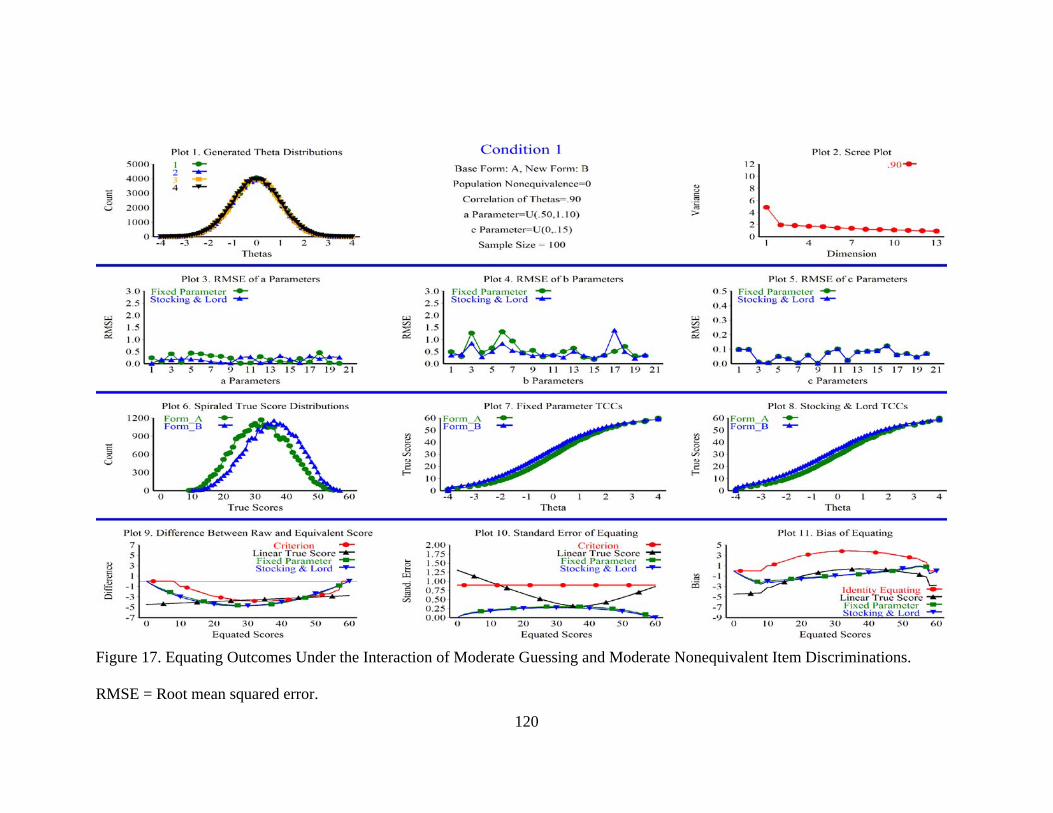
120

Figure 17. Equating Outcomes Under the Interaction of Moderate Guessing and Moderate Nonequivalent Item Discriminations.

RMSE = Root mean squared error.

121

Interactions of multidimensionality and population nonequivalence had little

direct effect on preequating error. When population nonequivalence and guessing

interacted, they tended to shrink the variance of the score distribution (compare plot 6 in

Figures 17 and Figure 18). The effect of this interaction was to lower the criterion for the

SEE (Plot 10). Otherwise, multidimensionality, population nonequivalence, and their

interactions with other factors had no significant negative effect on preequating in this

study.

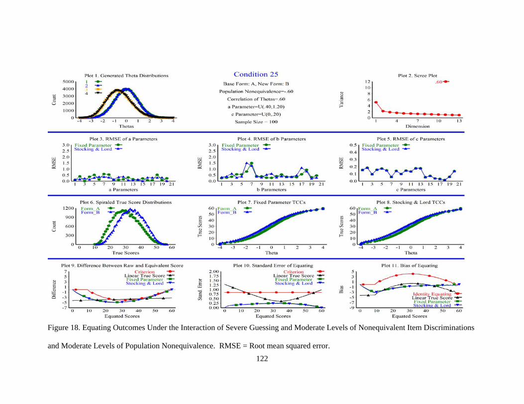
122

Figure 18. Equating Outcomes Under the Interaction of Severe Guessing and Moderate Levels of Nonequivalent Item Discriminations

and Moderate Levels of Population Nonequivalence. RMSE = Root mean squared error.

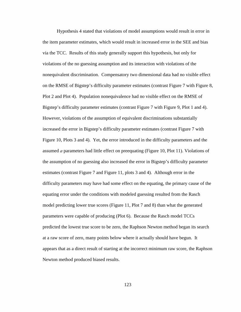
123

Hypothesis 4 stated that violations of model assumptions would result in error in

the item parameter estimates, which would result in increased error in the SEE and bias

via the TCC. Results of this study generally support this hypothesis, but only for

violations of the no guessing assumption and its interaction with violations of the

nonequivalent discrimination. Compensatory two dimensional data had no visible effect

on the RMSE of Bigstep’s difficulty parameter estimates (contrast Figure 7 with Figure 8,

Plot 2 and Plot 4). Population nonequivalence had no visible effect on the RMSE of

Bigstep’s difficulty parameter estimates (contrast Figure 7 with Figure 9, Plot 1 and 4).

However, violations of the assumption of equivalent discriminations substantially

increased the error in Bigstep’s difficulty parameter estimates (contrast Figure 7 with

Figure 10, Plots 3 and 4). Yet, the error introduced in the difficulty parameters and the

assumed a parameters had little effect on preequating (Figure 10, Plot 11). Violations of

the assumption of no guessing also increased the error in Bigstep’s difficulty parameter

estimates (contrast Figure 7 and Figure 11, plots 3 and 4). Although error in the

difficulty parameters may have had some effect on the equating, the primary cause of the

equating error under the conditions with modeled guessing resulted from the Rasch

model predicting lower true scores (Figure 11, Plot 7 and 8) than what the generated

parameters were capable of producing (Plot 6). Because the Rasch model TCCs

predicted the lowest true score to be zero, the Raphson Newton method began its search

at a raw score of zero, many points below where it actually should have begun. It

appears that as a direct result of starting at the incorrect minimum raw score, the Raphson

Newton method produced biased results.

124

The bias introduced by guessing is a symptom of a more general problem in

Rasch true score preequating. Namely, the further away from zero that a raw score

distribution begins, the greater the bias. If the minimum raw score is close to zero, then

the bias remains local to very low scores; however, if the minimum raw score is distant

from zero, then bias spreads across the score continuum.

To investigate this more general problem further, I produced a condition with no

violated assumptions, except that the test form was very easy relative to the ability of the

population (Figure 19). Using a form so mismatched to the ability of the population is

not considered good practice, but in some testing contexts, low scores are not common.

Although not shown, the Test Information Function would not be well aligned with the

ability distribution of the examinees. This condition produced a negatively skewed score

distribution (Plot 6), which resulted in a minimum raw score of ten points. This

condition created the same type of equating bias at the low end of the score range (Plot

11) that guessing produced. These results clearly show that it is not guessing alone that

can cause equating bias at the extremes of a score scale, but such bias will appear in

preequated conversion tables anytime the minimum or maximum raw score does not

match the minimum or maximum of the scale.

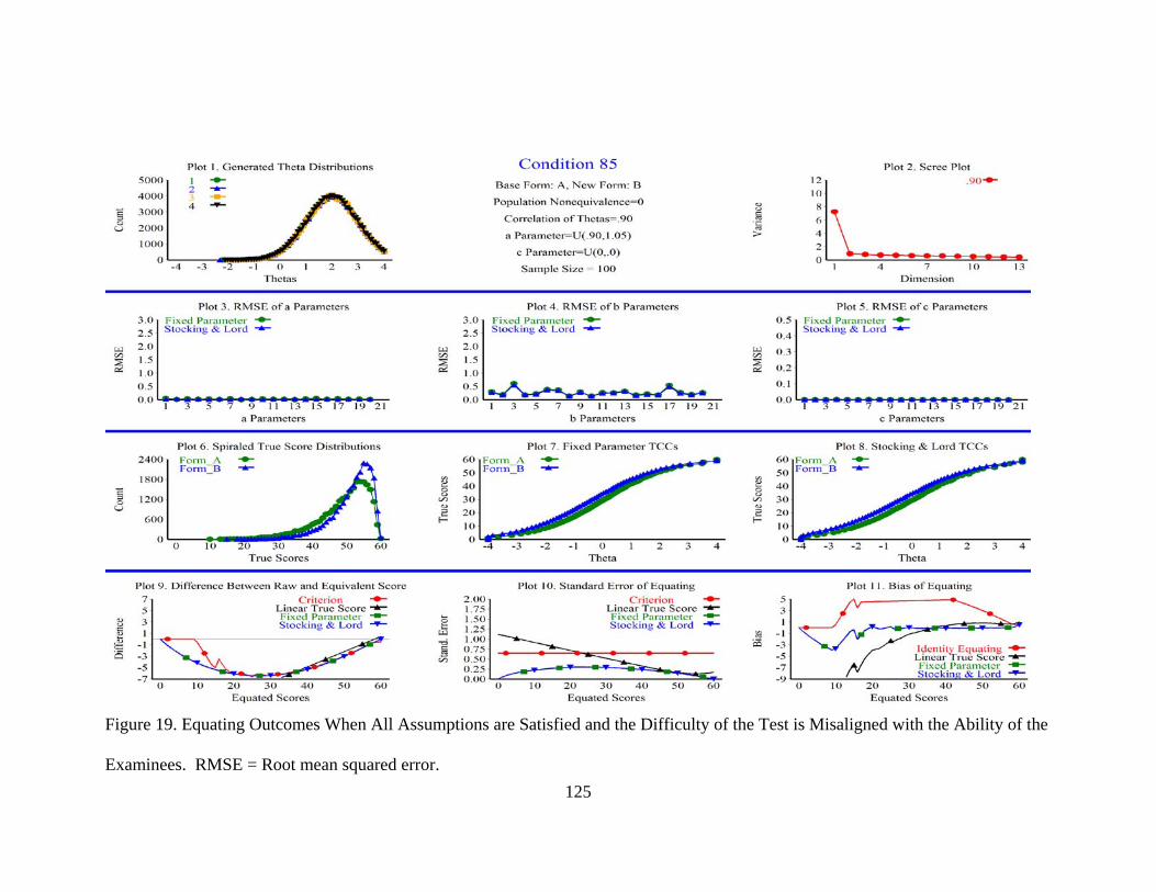
125

Figure 19. Equating Outcomes When All Assumptions are Satisfied and the Difficulty of the Test is Misaligned with the Ability of the

Examinees. RMSE = Root mean squared error.

126

In Rasch true score postequating, this problem could be addressed by starting the

Rapshon Newton procedure at the lowest raw score of the new form and then using

Kolen’s ad hoc procedure (Kolen & Brennan, 2004) to estimate equivalents between the

minimum raw score and all incorrect raw score. However, in a preequating context, the

minimum raw score is unknown. Using estimates for the pseudo-guessing parameter

would probably be the best approach to this problem. Other solutions to this problem may

be possible.

These results have implications for testing programs that use Rasch true score

equivalent scores to classify examinees. If guessing is present and/or the test forms are

not well matched to the ability of examinees, classification inaccuracy will probably

increase under preequating. Classification inaccuracy will probably increase because cut

scores for standards are usually defined on the first form produced for a testing program.

Bias in the equating would underestimate or overestimate equivalent scores of examinees

around the cut score, thereby creating incorrect classification decisions. The magnitude

of bias and classification inaccuracy would likely be consistent across forms to the extent

that the forms are parallel and the population is stable. Because relatively easier new

forms, produce equivalent scores that are negatively biased, easier forms would tend to

increase false negative decisions at the cut score.

Consistency of classification would not be affected as much by high minimum

raw scores induced by guessing or easy forms as would classification accuracy. It is

likely that examinees would all be affected in a similar manner by the bias observed in

this study. Relative to large sample equipercentile equating, low ability examinees would

receive lower equated scores caused by the bias introduced via high minimum raw scores

127

induced by guessing and easy forms. If a pilot study was conducted for the purpose of

defining a cut score, and then classification decisions began with the second form, then

all classified examinees would likely be classified consistently, provided test assembly

procedures are well defined and consistent. Otherwise, if the cut score is applied to

examinees from the first form, examinees around the cut score would likely be affected

differently in the first form than subsequent forms.

In general, accumulating item parameter error did increase preequating error

across four equatings, confirming hypothesis 5. The SEE increased in magnitude with

each new equating, although rarely exceeding the criterion by the fifth form. The bias

was less predictable than the SEE. The bias was not constant across multiple equatings,

sometimes increasing, and sometimes decreasing.

Recommendations

Based on the results of this study, Rasch true score preequating can be

recommended for sample sizes of 100 or more, provided that precision and accuracy is

required only around the mean of the score distribution, and provided that only two forms

are being equated. As violations of model assumptions increase and the item bank

increases, random error can quickly accumulate to produce high levels of SEE. To

prevent this, items in the pool could be recalibrated as the sample sizes grow, thereby

keeping random equating error in check. Even under violated conditions, Rasch true

score preequating generally produced better equating results than identity or linear

equating. For instance, criterion referenced tests that have cut scores high in the scale

score would be appropriate tests to use with Rasch true score preequating. Results of this

128

study do support the use of measuring growth via true score postequating, provided that

Kolen’s ad hoc procedure is used to produce equivalent scores between all incorrect and

the lowest raw score. Results from this study do not support the use of Rasch true score

preequating for tests that do not produce scores at or near zero and that require accuracy

at the extremes of the score scale. If accuracy all along the score scale is needed and if

raw scores of zero are unlikely, then Rasch true score preequating should not be used. If

accuracy and precision is needed all along the score continuum, then one may use the

3PL model if sample sizes permit it. Rasch true score postequating with Kolen’s ad hoc

procedure is a better alternative to preequating when accuracy is needed all along the

score scale.

Although sample size was not manipulated in this study, inferences can be made

concerning sample size. If at all possible, sample sizes of 500 should be used in Rasch

true score equating, especially if guessing is known to be present. To a limited extent,

the effects of violations of IRT assumptions on the RMSE of equating can be offset by

increasing the sample size from 100 to 500, thereby reducing the random component of

equating error. Not only would the larger sample size offset a small portion of the

equating bias, but a larger sample size will help to keep the SEE in check across multiple

equatings.

Results of this study support the use of either FPC or SCSL in developing a

calibrated item bank. FPC has a cost advantage over SCSL, since SCSL requires the use

of additional software and expertise in item linking. In contrast, FPC offers the

advantage of using the same software to estimate and calibrate the items in the bank,

saving considerable time, effort, and cost. However, this cost savings is lost if DIF

129

analysis is performed during the equating process, since DIF analysis requires two sets of

item parameter estimates. DIF analysis is recognized as a best practice, as a means of

screening common items during the equating process (Kolen & Brennan, 2004). Also, a

limitation of this study was that the TCCs were mostly parallel. If the TCCs were not

parallel, the SCSL method may produce better results than the FPC method, since the

SCSL accommodates mean differences in the a parameter between forms, and the FPC

method always assumes the a parameter is equal to one, both within and across forms.

So, this study demonstrated that FPC is a viable procedure on its own for parallel TCCs,

but if TCCs are not parallel, or if DIF analysis is to be performed, separate calibration

may be the best alternative, since it provides two sets of estimates for each item.

There are both advantages and disadvantages to implementing preequating. The

primary advantage to using preequating is that scores can be released immediately at the

end of the test administration. However, a disadvantage to reporting scores immediately,

is that no review of the items can be conducted after the test is administered. Therefore,

to prevent any unexpected problems with items, careful attention should be given to the

appearance of items to ensure that they are presented identically to past presentations of

the items. Also, it is advisable to keep items in relatively the same position across forms

(Kolen & Brennan, 2004). Moreover items used for scoring and calibration purposes

should be carefully selected for the property of population invariance. All of these

safeguards should reduce the risk of items performing differently than expected. Even

still, it is advisable to implement preequating with a postequating design and inspect the

performance of the method for a time period, before replacing postequating with

preequating to a calibrated item bank (Kolen & Brennan, 2004).

130

Limitations

As previously stated, to make this study feasible many factors that would likely

affect the performance of preequating have been held constant. Item parameter drift was

not an active variable, although in a real world context, items do tend to drift both

nonuniformly and uniformly. While studies have suggested that item parameter drift has

negligible effects on normal equating (Wells, Subkoviak, & Serlin, 2002), item parameter

drift may have a strong negative effect on preequating since preequating depends on

precalibrated items. In order for the results of this study to hold, parameter drift may

have to be minimal or all together absent. The effects of parameter drift on equating

could be the focus of a future study.

This study used 20 items as pilot items during each administration; as a result, a

large number of items (60) are shared in common between forms. Having a maximum

number of common items is ideal for CINEG equating and in fact was chosen for this

reason, but may not be typical. Many linking designs require a minimum of common

items between forms so as to minimize item exposure. Researchers should take care not

to assume that the results of this study will apply to test forms that share a moderate to

minimum number of common items (i.e., 20% to 50%).

Item context effects also pose a major threat to preequating (Kolen & Brennan,

2004). This study did not manipulate item context effects, so, the results generalize to

items that are not susceptible to item context effects. In order to use Rasch preequating

successfully, practitioners should exclude common items that show any susceptibility to

context effects.

In this study unrounded equivalent raw scores were used in calculating random

131

error and systematic error. Standard errors of rounded raw scores or scales scores could

also have been used to evaluate preequating. The drawback to using scale scores is that

they are very specific to a testing program, and so results do not generalize well to other

programs with different scales. However, the SEE of scale scores will be larger than

those of unrounded equivalent scores.

Another limitation to the study is the fact that test form similarity was not

manipulated. The magnitude of the difference between the forms was held constant. The

magnitude of the shift in the difficulty parameters was quite large (-.50 standard

deviations), so I suspect that most item banks would be able to produce forms less

dissimilar as this. The TCCs were also mostly parallel. If the average discrimination of

two forms differed substantially, then the results may not apply. In that situation, the

SCSL method may produce better results than the FPC method, since the SCSL

accommodates mean differences in item discriminations between forms.

A two dimensional compensatory model was used to simulate violations of

unidimensionality. More than three dimensions may produce different results. The use

of a noncompensatory model may have resulted in a different outcome as well. This

study examined two dimensional tests with a simple structure, in that subtest one scores

depended exclusively on dimension one, and subtest two scores depended exclusively on

dimension two. However, a test could be multidimensional in other ways, such as when a

positive response to an individual item depends on multiple dimensions.

132

Future research

Because this study used a true experimental design, it attains a high degree of

internal validity; however, simulation studies are sometimes criticized for having low

external validity, since real data are not used. It could be argued that this study achieved

a higher level of realism than most simulation studies, since four factors were

manipulated simultaneously to produce multiple, concurrent model violations.

Nonetheless, it would be advisable to perform additional research using actual data to

validate the feasibility of Rasch true score preequating.

Applying different equating criteria to the simulation results may have produced

different interpretations of the outcomes. A follow up study could be performed to

investigate the effectiveness of Rasch preequating using Lord’s equity criteria. While

this study focused on the limitations of Rasch preequating, other studies could focus on

strategies to extend the limitations defined by this study. For instance, Kolen and

Brennan have suggested the use of double linkings as a strategy to reduce the SEE (Kolen

& Brennan, 2004). Another study could examine the effect of using double or triple links

on the SEE across multiple equatings.

Another line of inquiry could examine the effect of repeating examinees on Rasch

preequating. Repeating examinees would likely alter the score distribution over time and

may represent an additional source of error in the item bank.

A logical extension of this study would be to vary the number of common items

used across forms, and vary the length of the test. As mentioned in the literature review

of this paper, prior studies have suggested that equating results largely depend on the

number and quality of common items. Since the current study used a relatively large

133

number of common items, it would be valuable to know if the findings of this study hold

true even when operational forms contain as few as 20 percent of the operational items in

common. It also would be interesting to see if these results hold true with very short or

very long tests.

Since high minimum raw scores induced by guessing or very easy tests, proved to

be the biggest threat to the accuracy of true score equating with the Rapshon Newton

method, a follow up study could be performed to investigate alternative approaches to

dealing with minimum raw scores that are distant from zero. Kolen devised an ad hoc

procedure for the 3PL model, using linear interpolation to extend the conversion table to

scores between the sum of the c parameters and all incorrect raw scores (Kolen &

Brennan, 2004). A new procedure needs to be developed that can accommodate score

distributions that do not extend to all incorrect raw scores for a preequating context. For

instance, would preequating results improve if the Rapshon Newton procedure was set to

start at the minimum raw score of the base form distribution, rather than zero? In this

same line of thinking, would a constant c parameter improve true score equating?

Empirical work can be performed on strategies to obtain a good constant c parameter

estimate under small sample sizes. It appears to me that any improvement to the false

assumption that the c parameter equals zero, would improve preequating results. This

leads me to believe that an IRT model that assumes equivalent a parameters, models b

parameters, and models a constant c parameter, may produce better preequating results

than Rasch preequating.

134

Conclusion

For those who use the Rasch model, this study offers insight into the limitations

of true score preequating. Rasch preequating will not produce accurate equating at the

extremes of the score scale, if the range of the scores do not extend across the entire score

continuum. This scenario can be caused by guessing or by forms that are not well

matched to the ability of the examinees. The bias at the extremes of a score scale may be

irrelevant to testing programs that use scores for pass/fail decisions, especially if the cut

score is close to the mean of the distribution. If a program requires accurate equating all

along the score scale, Rasch true score postequating with the Rapshon Newton method

will likely produce accurate results, provided the Raphson Newton method starts at the

minimum raw score rather than zero. The FPC method is a cost efficient and effective

approach to building the calibrated item bank, but separate calibration may be the best

calibration choice to facilitate DIF analysis in the equating process.

135

REFERENCES

American Educational Research Association, American Psychological Association, &

National Council on Measurement in Education, (1999). Standards for

Educational and Psychological Testing. Washington, DC: American Educational

Research Association.

Angoff, W.H. (1971). Scales, norms, and equivalent scores. In R.L. Thorndike (Ed.),

Educational measurement (2nd ed.) (pp. 508 – 600). Washington, DC: American

Council of Education.

Angoff, W.H. (1987). Technical and practical issues in equating: A discussion of four

papers. Applied Psychological Measurement, 11, 291-300.

Arce-Ferre, A.J., (2008). Comparing screening approaches to investigate stability of

common items in Rasch equating. Journal of Applied Measurement, 9(1), 57-67.

Baker, F.B., & AL-Karni, A. (1991). A comparison of two procedures for computing IRT

equating coefficients. Journal of Educational Measurement, 28, 147-162.

Ban, J.C., Hanson, B. A., Wang, T., Yi, Q., & Harris, D. J. (2001). A comparative study

of on-line pretest-item calibration/scaling methods in computerized adaptive

testing. Journal of Educational Measurement, 38, 191–212.

136

Beguin, A.A., Hanson, B.A., & Glas, C.A.W. (2000, April). Effect of

Multidimensionality on Separate and Concurrent Estimation in IRT Equating.

Paper presented at the Educational Research Association, New Orleans, L.A.

Bejar, I.I. & Wingersky, M.S. (1982). A study of preequating based on item response

theory, Applied Psychological Measurement, 6(3), 309 – 325.

Bogan, E.D. & Yen,W.M. (1983). Detecting multidimensionality and examining its

effects on vertical equating with the three-parameter logistic model. Monterey,

CA: CTB/ McGraw-Hill. (ERIC document Reproduction Service No. ED229450).

Bogan, E.D., & Yen, W.M. (1983, April). Detecting multidimensionality and examining

its effects on vertical equating the three parameter logistic model. Monterey, CA:

CTB/McGraw-Hill. (ERIC Document Reproduction Service No. ED229450).

Bolt, D.M., (1999). Evaluating the effects of multidimensionality on IRT true-score

equating. Applied Measurement in Education, 12(4), 383-407.

Bond, T.G., & Fox, C.M. (2001). Applying the Rasch Model: Fundamental

Measurement in the Human Sciences. Mahwah, NJ: Lawrence Erlbaum

Associates.

Briggs, D.C., Wilson, M. (2006). An Introduction to Multidimensional Measurement

Using Rasch Models. In Smith, E.V. & Smith R.M. (Eds.) Introduction to Rasch

Measurement. Maple Grove, Minn: JAM press.

Camili,G., Wang,M.M. & Fesq, J., (1995). The effects of dimensionality on equating the

Law School Admission Test. Journal of Educational Measurement, 1, 79-96.

137

Cizek, G.J., (2001, April). An Overview of Issues Concerning Cheating on Large-Scale

Tests. Paper presented at the annual meeting of the National Council on

Measurement in Education, Seattle, WA.

Cook, L.L. & Petersen, N.S. (1987). Problems related to the use of conventional and

item response theory equating method in less than optimal circumstances.

Applied Psychological Measurement, 11, 225-244.

Cook, L.L., Douglass, Dorans, N.J., Eignor, D.R., & Petersen, N.S. (1985). An

assessment of the relationship between the assumption of unidimensionality and

the quality of IRT true-score equating. (ETS Research Report NO. RR-85-30).

Princeton, NJ: Educational Testing Service.

Crocker, L. & Algina, J. (1986). Introduction to classical and modern test theory.

Belmont, CA: The Wadsworth Group.

De Camplain, A.F. (1996). The effect of multidimensionality on IRT true-score equating

for subgroups of examinees. Journal of Educational Measurement, 33(2), 181-

201.

DeMars, C., (2002). Incomplete data and item parameter estimates under JMLE and

MML estimation. Applied Measurement in Education, 15(1), 15-31.

Divgi, D.R. (1986). Does the Rasch model really work for multiple-choice items? Not if

you look closely. Journal of Educational Measurement, 23, 283-298.

Domaleski, C.S., (2006). Exploring the efficacy of pre-equating a large scale criterion-

referenced assessment with respect to measurement equivalence. Published

doctoral dissertation, Ann Arbor, MI: ProQuest Information and Learning

Company.

138

Dorans, N. & Kingston, N. (1985). The effects of violations of unidimensionality on the

estimations of item and ability parameters on item response theory equating of the

GRE verbal scale, Journal of Educational Measurement, 22(4), 249-262.

Dorans, N.J. & Kingston, N.M. (1985). The effects of violations of unidimensionality on

the estimation of item and ability parameters and on item response theory

equating of the GRE verbal scale. Journal of Educational Measurement, 22(4),

249–262.

Dorans, N.J. (2004). Equating, concordance, and expectation. Applied Psychological

Measurement, 28(4), 227–246.

Du, Z., Lipkins, R.H., and Jones, J.P. (2002). Evaluating the adequacy of using IRT

models for pre-equating a computer-based national licensing examination. Paper

presented at the Annual Meeting of the American Educational Research

Association, New Orleans, LA.

Eignor, D.R. & Stocking, M.L. (1986). An investigation of the possible causes for the

inadequacy of IRT preequating (Research Report 86-14). Princeton, NJ:

Educational Testing Service.

Eignor, D.R. (1985). An investigation of the feasibility and practical outcomes of

preequating the SAT verbal and mathematical sections (Research Report 86-14).

Princeton, NJ: Educational Testing Service.

Fan, X. & Fan, X. (2005). Using SAS for monte carlo simulation research in SEM.

Structural Equation Modeling, 12(2), 299-333.

139

Feuer, M.J., Holland, P.W., Green, B.F., Bertenthal, M.W., & Hemphill, F.C. (Eds.).

(1999). Uncommon measures: Equivalence and linkage among educational tests

(Report of the Committee on Equivalency and Linkage of Educational Tests,

National Research Council). Washington, DC: National Academy Press.

Forsyth, R., Saisangijan,U., & Gilmer, J. (1981). Some empirical results related to the

robustness of the Rasch model. Applied Psychological Measurement, 5, 175-186.

Gustaffson, J.E. (1980). Testing and obtaining fit of data to the Rasch model. British

Journal of Mathematical and Statistical Psychology, 33, 205-233.

Hambleton, R.K. & Swaminathan, H. (1985). Item response theory: Principles and

applications. Boston: Kluwer.

Han, K. (2007). Wingen2 (Version 2.5.4.414). [Computer program]. Amherst, MA:

University of Massachusetts, School of Education. Retrieved from

http://www.umass.edu/remp/ software/ wingen/homeL.html.

Hanson, B.A, & Beguin, A.A. (2002). Obtaining a common scale for item response

theory item parameters using separate versus concurrent estimation in the

common-item equating design. Applied Psychological Measurement, 26(1), 3-24.

Hanson, B.A., (2002). IRT command language (version 0.020301). Monterey, CA:

Author.

Harris, D.J. (1991). Practical implications of the context effects resulting from the use of

scrambled test forms. Paper presented at the annual meeting of the American

Educational Research Association, Chicago.

Hendrickson, A.B., & Kolen, M.J. (1999, October) IRT equating of the MCAT. Report

140

prepared under contract with the Association of American Medical Colleges for

the Medical College Admissions Test (MCAT) Graduate Student Research

Program, Washington, D.C.

Hills, J.R., Subhiyah, R.G., and Hirsch, T.M. (1988). Equating minimum-competency

tests: Comparisons of methods. Journal of Educational Measurement, 25, 221-

231.

Holland, P.W. & Dorans, N.J. (2006). Linking and Equating. In R.L. Brennan. (Ed.),

Educational Measurement (4th ed.). (pp. 187-220). Westport, CT: American

Council on Education and Praeger Publishers.

Holmes, S. E. (1982). Unidimensionality and vertical equating with the Rasch model.

Journal of Educational Measurement, 19, 139-147.

Jodoin, M. G., Keller, L. A., & Swaminathan, H. (2003). A comparison of linear, fixed

common item, and concurrent parameter estimation equating procedures in

capturing academic growth. The Journal of Experimental Education, 71, 229–

250.

Kaskowitz, G.S., & De Ayala, R.J. (2001). The effect of error in item parameter

estimates on the test response function method of linking. Applied Psychological

Measurement, 25(1), 39-52.

Kim, S, (2006). A Comparative Study of IRT FPC Methods. Journal of Educational

Measurement, 43(4), 355–381.

141

Kim, S. & Kolen, M., (2003). Program for polytomous IRT scale transformation.

[Computer program]. Retrieved from

http://www.education.uiowa.edu/casma/Equating LinkingPrograms.htm

Kim, S. -H., & Cohen, A. S. (1998). A comparison of linking and concurrent calibration

under item response theory. Applied Psychological Measurement, 22, 131-143.

Kim, S., & Kolen, M.J. (2006). Effects on scale linking of different definitions of

criterion functions for the IRT characteristic curve methods. Journal of

educational and behavioral statistics, 32(4), 371-397.

Kolen, M. & Cui, Z., (2004). POLYEQUATE. [Computer program]. Retrieved from

http://www.education.uiowa.edu/casma/EquatingLinkingPrograms.htm.

Kolen, M., Hanson, B., Cui, Z., Chien, Y. & Zeng, (2004). RAGE-RGEQUATEv3.

[Computer program]. Retrieved from http://www.education.uiowa.edu

/casma/EquatingLinkingPrograms.htm.

Kolen, M.J., & Brennan, R.L. (2004). Test Equating, Scaling, and Linking: Methods and

Practices (2nd ed.). New York: Springer –Verlag.

Kolen, M.J., & Harris, D.J. (1990). Comparison of item preequating and random groups

equating using IRT and equipercentile methods. Journal of Educational

Measurement, 27, 27-39.

Lee, H. & Terry, R. (2005). MDIRT-FIT: SAS macros for fitting multidimensional item

response theory (IRT) Models. Paper presented at the SAS Users Group

International. SUGI paper (199-31).

142

Li, Y. & Lissitz, R. W. (2000). An evaluation of multidimensional IRT equating methods

by assessing the accuracy of transforming parameters onto a target test metric.

Applied Psychological Measurement, 24(2), 115-138.

Li, Y.H., Griffith, W.D., & Tam, H.P. (1997, June). Equating multiple tests via an IRT

linking design: Utilizing a single set of anchor items with fixed common item

parameters during the calibration process. Paper presented at the annual meeting

of the Psychometric Society, Knoxville, TN.

Li, Y.H., Tam, H.P., & Tompkins, L.J. (2004). A comparison of using the fixed

common-precalibrated parameter method and the matched characteristic curve

method for linking multiple test items. International Journal of Testing, 4(3), 267-

293.

Linacre, J.M, & Wright, B.D., (1998). A user’s guide to BIGSTEPS. Chicago: Retrieved

from www.Winsteps.com.

Linacre, J.M, & Wright, B.D., (1998). BIGSTEPS. [Computer program]. Chicago:

Retrieved from www.Winsteps.com.

Livingston, L. (2004). Equating Test Scores (Without IRT). Princeton, NJ: Educational

Testing.

Lord, F., & Novick, M. (1968). Statistical Theories of Mental Test Scores. Reading, MA:

Addison-Wesley.

Loyd, B.H., & Hoover, H.D. (1981). Vertical equating using the Rasch model. Journal

of Educational Measurement, 17, 179-193.

143

Michaelides, M.P., Haertel, E.H. (2004). Sampling of Common Items: An unrecognized

Source of Error in Test Equating. Los Angeles, University of California, Center

for the Study of Evaluation (CSE).

Michealides, M.P. (2003). Sensitivity of IRT Equating to the Behavior of Test Equating

Items. paper presented at the Annual Meeting of the Educational Research

Association, Chicago, Illinois.

Mislevy, R. J. (1982, March). Five Steps Toward Controlling Item Parameter Drift.

Paper presented at the annual meeting of the American Educational Research

Association, New York.

Mislevy, Robert J. (1992). Linking educational assessments: concepts, issues, methods,

and prospects. Princeton, NJ: Educational Testing Service.

Moses, T., Yang,W.L., and Wilson, C. (2007). Using kernel equating to assess item order

effects on test scores, Journal of Educational Measurement, 44(2), 157-178.

Motika, R. (2003). Effects of Anchor Items Content Representation on the Accuracy and

Precision of Small Sample Linear Test Equating. Doctoral Dissertation.

University of South Florida.

Paek, I. & Young,M. (2005). Investigation of student growth recovery in a fixed-item

linking procedure with a fixed-person prior distribution for mixed-format test

data, Applied Measurement in Education, 18(2), 199 – 215.

Parshall, C.G., Houghton, P.D., & Kromrey, J.D. (1995). Equating error and statistical

bias in small sample linear equating. Journal of Educational Measurement, 32(1),

37-54.

Pomplun, M., Omar, H., & Custer, M. (2004). A Comparison of Winsteps and Bilog-MG

144

for Vertical Scaling with the Rasch Model. Educational and Psychological

Measurement, 64, 600 – 616.

Prowker, A.N., (2005). Long term stability of fixed common item parameter equating:

what no child left behind could mean for equating practices. Published doctoral

dissertation, Ann Arbor, MI: ProQuest Information and Learning Company.

Raju, N.S., Edwards, J.E. and Osberge, D.W. (1983). The effect of anchor test size in

vertical equating with the Rasch and three-parameter models. Paper presented at

the Annual Meeting of the National Council on Measurement in Education,

Montreal, Canada.

Reckase, M. D. (1985, April). The difficulty of test items that measure more than one

ability. Paper presented at the annual meeting of the American Educational

Research Association, Chicago, IL.

Reckase, M., Ackerman, T. & Carlson, J. (1988). Building a unidimensional test using

multidimensional items, Journal of Educational Measurement, 25(3), 193-203.

Skaggs, G., & Lissetz, R.W. (1986). Test equating: relevant issues and review of recent

research. Review of Educational Research, 56(4), 495-529.

Slinde, J.A., & Linn, R.L. (1978). An exploration of the adequacy of the Rasch model

for the problem of vertical equating, Journal of Educational Measurement, 15,

23-35.

Stocking, M.L., & Lord, F.M. (1983). Developing a common metric in item response

theory. Applied Psychological Measurement, 14, 299-311.

Stocking, M.L., & Lord, F.M., (1986). The impact of different ability distributions on

145

IRT preequating, (Research Report 86-49). Princeton, NJ: Educational Testing

Service.

Tsai, T., Hanson, B., Kolen, M.J. & Forsyth, R.A. (2001). A comparison of bootstrap

standard errors of IRT equating methods for the common-item nonequivalent

groups design, Applied Measurement in Education, 14(1) 17-30.

Von Davier, A., Holland, P.W., and Thayer, D.T. (2004) The Kernel Method of Test

Equating. New York: Springer-Verlag.

Wang, M.M. (1985). Fitting a undimensinal model to multidimensional item response

data: The effects of latent space misspecification on the application of IRT.

Unpublished doctoral dissertation, University of Iowa, Iowa City.

Wells, C., Subkoviak, M., & Serlin, R. (2002). The effect of item parameter drift on

examinee ability estimates, Applied Psychological Measurement, 26(1), 77-87.

Williams, V.S.L., Pommerich, M., & Thissen, D. (1998). A comparison of developmental

scales based on Thurstone methods and item response theory, Journal of

Educational Measurement, 35, 93-107.

Wilson, M. (2004). On choosing a model for measuring. In Smith, E.V. & Smith R.M.

(Eds.), Introduction to Rasch Measurement. Maple Grove, Minn: JAM press.

Wingersky, M.S., and Lord, F.M. (1984). An investigation of methods for reducing

sampling error in certain IRT procedures. Applied Psychological Measurement,

21, 331-345.

Wolfe, E.W. (2006). Equating and item banking with the Rasch model. In Smith, E.V.

& Smith R.M. (Eds.) Introduction to Rasch Measurement. Maple Grove, Minn:

146

JAM press.

Wollack, J. A., Sung, H. J., & Kang, T. (2006, April). The Impact of Compounding Item

Parameter Drift on Ability Estimation. Paper presented at the annual meeting of

the National Council on Measurement in Education, San Francisco, CA.

Wright, B.D., & Bell, S.R. (1984). Item banks: What, why, how. Journal of Educational

Measurement, 21, 331-345.

Yen, W. & Fitzpatrick, A. (2006). Item Response Theory. In R.L. Brennan. (Ed.),

Educational Measurement (4th ed.). (pp. 111-153). Westport, CT: American

Council on Education and Praeger Publishers.

Yen,W.M.(1984). Effects of local item dependence on the fit and equating performance

of the three parameter logistic model, Applied Psychological Measurement, 2,

125-145.

Yu, C. & Popp, S. (2005). Test Equating by Common Items and Common Subjects:

Concepts and Applications, Practical Assessment, Research and Evaluation,

10(4), 1-19.

Zenisky, A.L. (2001, October). Investigating the Accumulation of Equating Error in

Fixed Common Item Parameter Linking: A Simulation Study. Paper presented at

the annual meeting of the Northeaster Educational Research Association,

Kerhonkson, NY.

Zwick, R.(1991). Effects of item order and context on the estimation of NAEP reading

proficiency. Educational Measurement: Issues and Practices, 10, 10-16.

147

APPENDIX A: SAS CODE

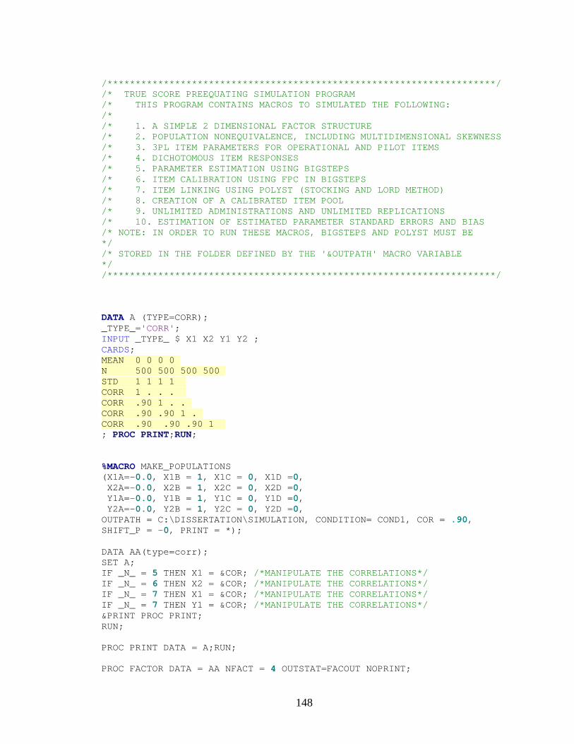
148

/*********************************************************************/ /* TRUE SCORE PREEQUATING SIMULATION PROGRAM /* THIS PROGRAM CONTAINS MACROS TO SIMULATED THE FOLLOWING: /* /* 1. A SIMPLE 2 DIMENSIONAL FACTOR STRUCTURE /* 2. POPULATION NONEQUIVALENCE, INCLUDING MULTIDIMENSIONAL SKEWNESS /* 3. 3PL ITEM PARAMETERS FOR OPERATIONAL AND PILOT ITEMS /* 4. DICHOTOMOUS ITEM RESPONSES /* 5. PARAMETER ESTIMATION USING BIGSTEPS /* 6. ITEM CALIBRATION USING FPC IN BIGSTEPS /* 7. ITEM LINKING USING POLYST (STOCKING AND LORD METHOD) /* 8. CREATION OF A CALIBRATED ITEM POOL /* 9. UNLIMITED ADMINISTRATIONS AND UNLIMITED REPLICATIONS /* 10. ESTIMATION OF ESTIMATED PARAMETER STANDARD ERRORS AND BIAS /* NOTE: IN ORDER TO RUN THESE MACROS, BIGSTEPS AND POLYST MUST BE */ /* STORED IN THE FOLDER DEFINED BY THE '&OUTPATH' MACRO VARIABLE */ /*********************************************************************/ DATA A (TYPE=CORR); _TYPE_='CORR'; INPUT _TYPE_ $ X1 X2 Y1 Y2 ; CARDS; MEAN 0 0 0 0 N 500 500 500 500 STD 1 1 1 1 CORR 1 . . . CORR .90 1 . . CORR .90 .90 1 . CORR .90 .90 .90 1 ; PROC PRINT;RUN; %MACRO MAKE_POPULATIONS (X1A=-0.0, X1B = 1, X1C = 0, X1D =0, X2A=-0.0, X2B = 1, X2C = 0, X2D =0, Y1A=-0.0, Y1B = 1, Y1C = 0, Y1D =0, Y2A=-0.0, Y2B = 1, Y2C = 0, Y2D =0, OUTPATH = C:\DISSERTATION\SIMULATION, CONDITION= COND1, COR = .90, SHIFT_P = -0, PRINT = *); DATA AA(type=corr); SET A; IF _N_ = 5 THEN X1 = &COR; /*MANIPULATE THE CORRELATIONS*/ IF _N_ = 6 THEN X2 = &COR; /*MANIPULATE THE CORRELATIONS*/ IF _N_ = 7 THEN X1 = &COR; /*MANIPULATE THE CORRELATIONS*/ IF _N_ = 7 THEN Y1 = &COR; /*MANIPULATE THE CORRELATIONS*/ &PRINT PROC PRINT; RUN; PROC PRINT DATA = A;RUN; PROC FACTOR DATA = AA NFACT = 4 OUTSTAT=FACOUT NOPRINT;

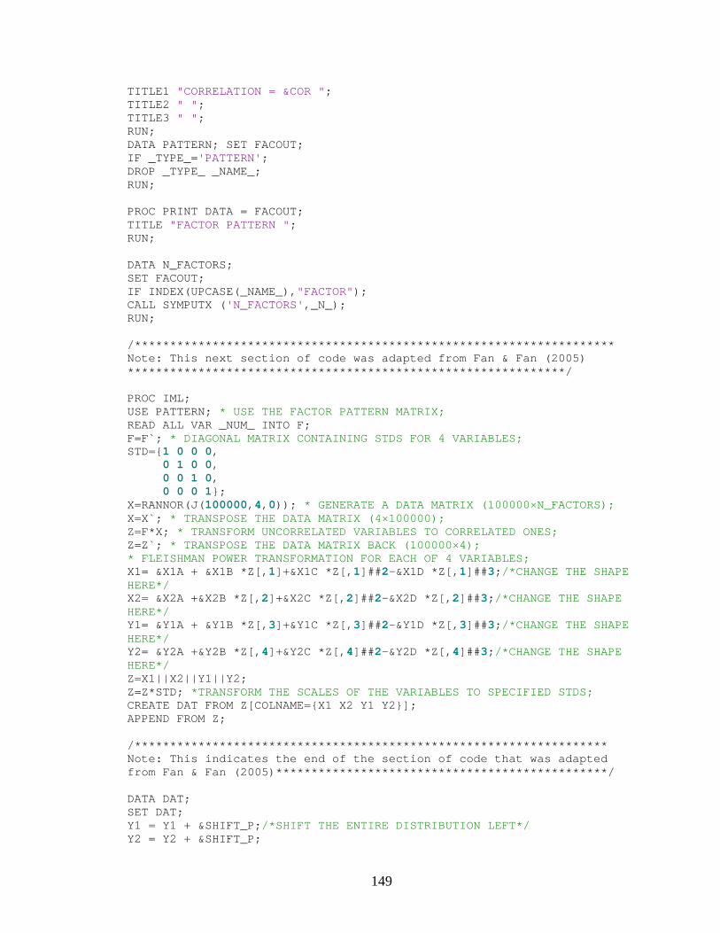
149

TITLE1 "CORRELATION = &COR "; TITLE2 " "; TITLE3 " "; RUN; DATA PATTERN; SET FACOUT; IF _TYPE_='PATTERN'; DROP _TYPE_ _NAME_; RUN; PROC PRINT DATA = FACOUT; TITLE "FACTOR PATTERN "; RUN; DATA N_FACTORS; SET FACOUT; IF INDEX(UPCASE(_NAME_),"FACTOR"); CALL SYMPUTX ('N_FACTORS',_N_); RUN; /******************************************************************** Note: This next section of code was adapted from Fan & Fan (2005) **************************************************************/ PROC IML; USE PATTERN; * USE THE FACTOR PATTERN MATRIX; READ ALL VAR _NUM_ INTO F; F=F`; * DIAGONAL MATRIX CONTAINING STDS FOR 4 VARIABLES; STD={1 0 0 0, 0 1 0 0, 0 0 1 0, 0 0 0 1}; X=RANNOR(J(100000,4,0)); * GENERATE A DATA MATRIX (100000×N_FACTORS); X=X`; * TRANSPOSE THE DATA MATRIX (4×100000); Z=F*X; * TRANSFORM UNCORRELATED VARIABLES TO CORRELATED ONES; Z=Z`; * TRANSPOSE THE DATA MATRIX BACK (100000×4); * FLEISHMAN POWER TRANSFORMATION FOR EACH OF 4 VARIABLES; X1= &X1A + &X1B *Z[,1]+&X1C *Z[,1]##2-&X1D *Z[,1]##3;/*CHANGE THE SHAPE HERE*/ X2= &X2A +&X2B *Z[,2]+&X2C *Z[,2]##2-&X2D *Z[,2]##3;/*CHANGE THE SHAPE HERE*/ Y1= &Y1A + &Y1B *Z[,3]+&Y1C *Z[,3]##2-&Y1D *Z[,3]##3;/*CHANGE THE SHAPE HERE*/ Y2= &Y2A +&Y2B *Z[,4]+&Y2C *Z[,4]##2-&Y2D *Z[,4]##3;/*CHANGE THE SHAPE HERE*/ Z=X1||X2||Y1||Y2; Z=Z*STD; *TRANSFORM THE SCALES OF THE VARIABLES TO SPECIFIED STDS; CREATE DAT FROM Z[COLNAME={X1 X2 Y1 Y2}]; APPEND FROM Z; /******************************************************************* Note: This indicates the end of the section of code that was adapted from Fan & Fan (2005)***********************************************/ DATA DAT; SET DAT; Y1 = Y1 + &SHIFT_P;/*SHIFT THE ENTIRE DISTRIBUTION LEFT*/ Y2 = Y2 + &SHIFT_P;

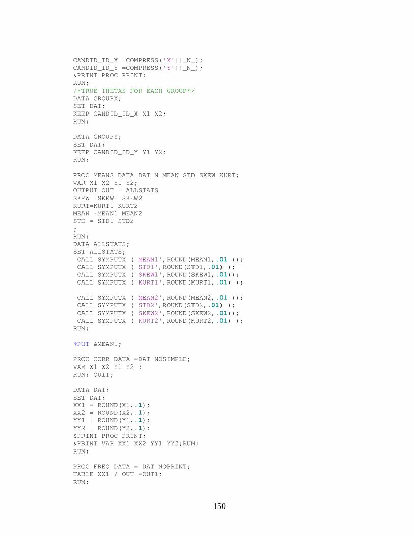
150

CANDID_ID_X =COMPRESS('X'||_N_); CANDID_ID_Y =COMPRESS('Y'||_N_); &PRINT PROC PRINT; RUN; /*TRUE THETAS FOR EACH GROUP*/ DATA GROUPX; SET DAT; KEEP CANDID_ID_X X1 X2; RUN; DATA GROUPY; SET DAT; KEEP CANDID_ID_Y Y1 Y2; RUN; PROC MEANS DATA=DAT N MEAN STD SKEW KURT; VAR X1 X2 Y1 Y2; OUTPUT OUT = ALLSTATS SKEW =SKEW1 SKEW2 KURT=KURT1 KURT2 MEAN =MEAN1 MEAN2 STD = STD1 STD2 ; RUN; DATA ALLSTATS; SET ALLSTATS; CALL SYMPUTX ('MEAN1',ROUND(MEAN1,.01 )); CALL SYMPUTX ('STD1',ROUND(STD1,.01) ); CALL SYMPUTX ('SKEW1',ROUND(SKEW1,.01)); CALL SYMPUTX ('KURT1',ROUND(KURT1,.01) ); CALL SYMPUTX ('MEAN2',ROUND(MEAN2,.01 )); CALL SYMPUTX ('STD2',ROUND(STD2,.01) ); CALL SYMPUTX ('SKEW2',ROUND(SKEW2,.01)); CALL SYMPUTX ('KURT2',ROUND(KURT2,.01) ); RUN; %PUT &MEAN1; PROC CORR DATA =DAT NOSIMPLE; VAR X1 X2 Y1 Y2 ; RUN; QUIT; DATA DAT; SET DAT; XX1 = ROUND(X1,.1); XX2 = ROUND(X2,.1); YY1 = ROUND(Y1,.1); YY2 = ROUND(Y2,.1); &PRINT PROC PRINT; &PRINT VAR XX1 XX2 YY1 YY2;RUN; RUN; PROC FREQ DATA = DAT NOPRINT; TABLE XX1 / OUT =OUT1; RUN;

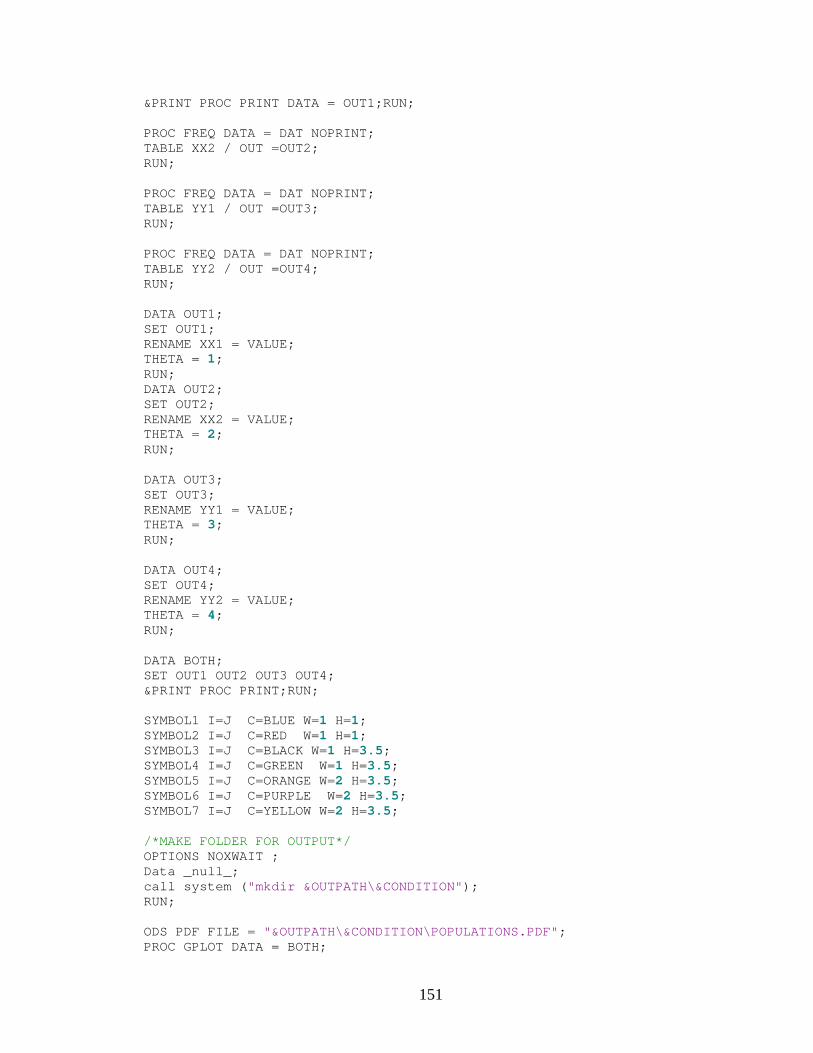
151

&PRINT PROC PRINT DATA = OUT1;RUN; PROC FREQ DATA = DAT NOPRINT; TABLE XX2 / OUT =OUT2; RUN; PROC FREQ DATA = DAT NOPRINT; TABLE YY1 / OUT =OUT3; RUN; PROC FREQ DATA = DAT NOPRINT; TABLE YY2 / OUT =OUT4; RUN; DATA OUT1; SET OUT1; RENAME XX1 = VALUE; THETA = 1; RUN; DATA OUT2; SET OUT2; RENAME XX2 = VALUE; THETA = 2; RUN; DATA OUT3; SET OUT3; RENAME YY1 = VALUE; THETA = 3; RUN; DATA OUT4; SET OUT4; RENAME YY2 = VALUE; THETA = 4; RUN; DATA BOTH; SET OUT1 OUT2 OUT3 OUT4; &PRINT PROC PRINT;RUN; SYMBOL1 I=J C=BLUE W=1 H=1; SYMBOL2 I=J C=RED W=1 H=1; SYMBOL3 I=J C=BLACK W=1 H=3.5; SYMBOL4 I=J C=GREEN W=1 H=3.5; SYMBOL5 I=J C=ORANGE W=2 H=3.5; SYMBOL6 I=J C=PURPLE W=2 H=3.5; SYMBOL7 I=J C=YELLOW W=2 H=3.5; /*MAKE FOLDER FOR OUTPUT*/ OPTIONS NOXWAIT ; Data _null_; call system ("mkdir &OUTPATH\&CONDITION"); RUN; ODS PDF FILE = "&OUTPATH\&CONDITION\POPULATIONS.PDF"; PROC GPLOT DATA = BOTH;

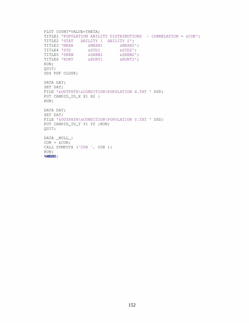
152

PLOT COUNT*VALUE=THETA; TITLE1 "POPULATION ABILITY DISTRIBUTIONS - CORRELATION = &COR"; TITLE2 "STAT ABILITY 1 ABILITY 2"; TITLE3 "MEAN &MEAN1 &MEAN2"; TITLE4 "STD &STD1 &STD2"; TITLE5 "SKEW &SKEW1 &SKEW2"; TITLE6 "KURT &KURT1 &KURT2"; RUN; QUIT; ODS PDF CLOSE; DATA DAT; SET DAT; FILE "&OUTPATH\&CONDITION\POPULATION X.TXT " DSD; PUT CANDID_ID_X X1 X2 ; RUN; DATA DAT; SET DAT; FILE "&OUTPATH\&CONDITION\POPULATION Y.TXT " DSD; PUT CANDID_ID_Y Y1 Y2 ;RUN; QUIT; DATA _NULL_; COR = &COR; CALL SYMPUTX ('COR ', COR ); RUN; %MEND;

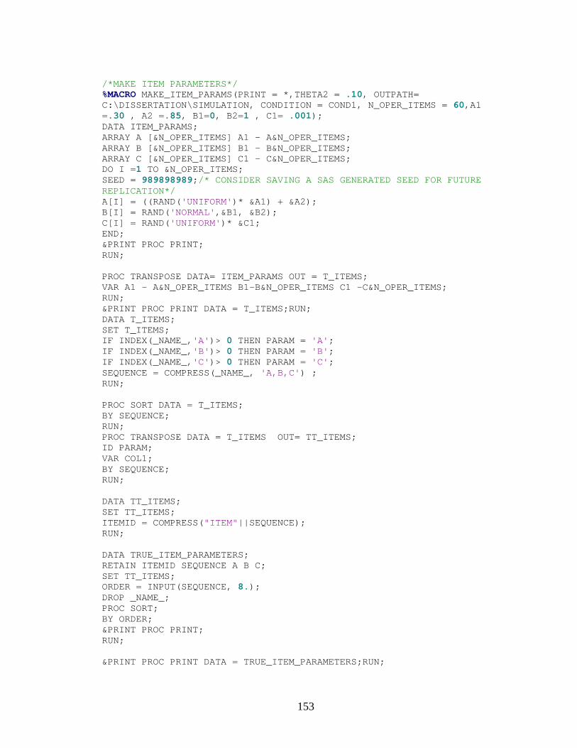
153

/*MAKE ITEM PARAMETERS*/ %MACRO MAKE_ITEM_PARAMS(PRINT = *,THETA2 = .10, OUTPATH= C:\DISSERTATION\SIMULATION, CONDITION = COND1, N_OPER_ITEMS = 60,A1 =.30 , A2 =.85, B1=0, B2=1 , C1= .001); DATA ITEM_PARAMS; ARRAY A [&N_OPER_ITEMS] A1 - A&N_OPER_ITEMS; ARRAY B [&N_OPER_ITEMS] B1 - B&N_OPER_ITEMS; ARRAY C [&N_OPER_ITEMS] C1 - C&N_OPER_ITEMS; DO I =1 TO &N_OPER_ITEMS; SEED = 989898989;/* CONSIDER SAVING A SAS GENERATED SEED FOR FUTURE REPLICATION*/ A[I] = ((RAND('UNIFORM')* &A1) + &A2); B[I] = RAND('NORMAL',&B1, &B2); C[I] = RAND('UNIFORM')* &C1; END; &PRINT PROC PRINT; RUN; PROC TRANSPOSE DATA= ITEM_PARAMS OUT = T_ITEMS; VAR A1 - A&N_OPER_ITEMS B1-B&N_OPER_ITEMS C1 -C&N_OPER_ITEMS; RUN; &PRINT PROC PRINT DATA = T_ITEMS;RUN; DATA T_ITEMS; SET T_ITEMS; IF INDEX(_NAME_,'A')> 0 THEN PARAM = 'A'; IF INDEX(_NAME_,'B')> 0 THEN PARAM = 'B'; IF INDEX(_NAME_,'C')> 0 THEN PARAM = 'C'; SEQUENCE = COMPRESS(_NAME_, 'A,B,C') ; RUN; PROC SORT DATA = T_ITEMS; BY SEQUENCE; RUN; PROC TRANSPOSE DATA = T_ITEMS OUT= TT_ITEMS; ID PARAM; VAR COL1; BY SEQUENCE; RUN; DATA TT_ITEMS; SET TT_ITEMS; ITEMID = COMPRESS("ITEM"||SEQUENCE); RUN; DATA TRUE_ITEM_PARAMETERS; RETAIN ITEMID SEQUENCE A B C; SET TT_ITEMS; ORDER = INPUT(SEQUENCE, 8.); DROP _NAME_; PROC SORT; BY ORDER; &PRINT PROC PRINT; RUN; &PRINT PROC PRINT DATA = TRUE_ITEM_PARAMETERS;RUN;

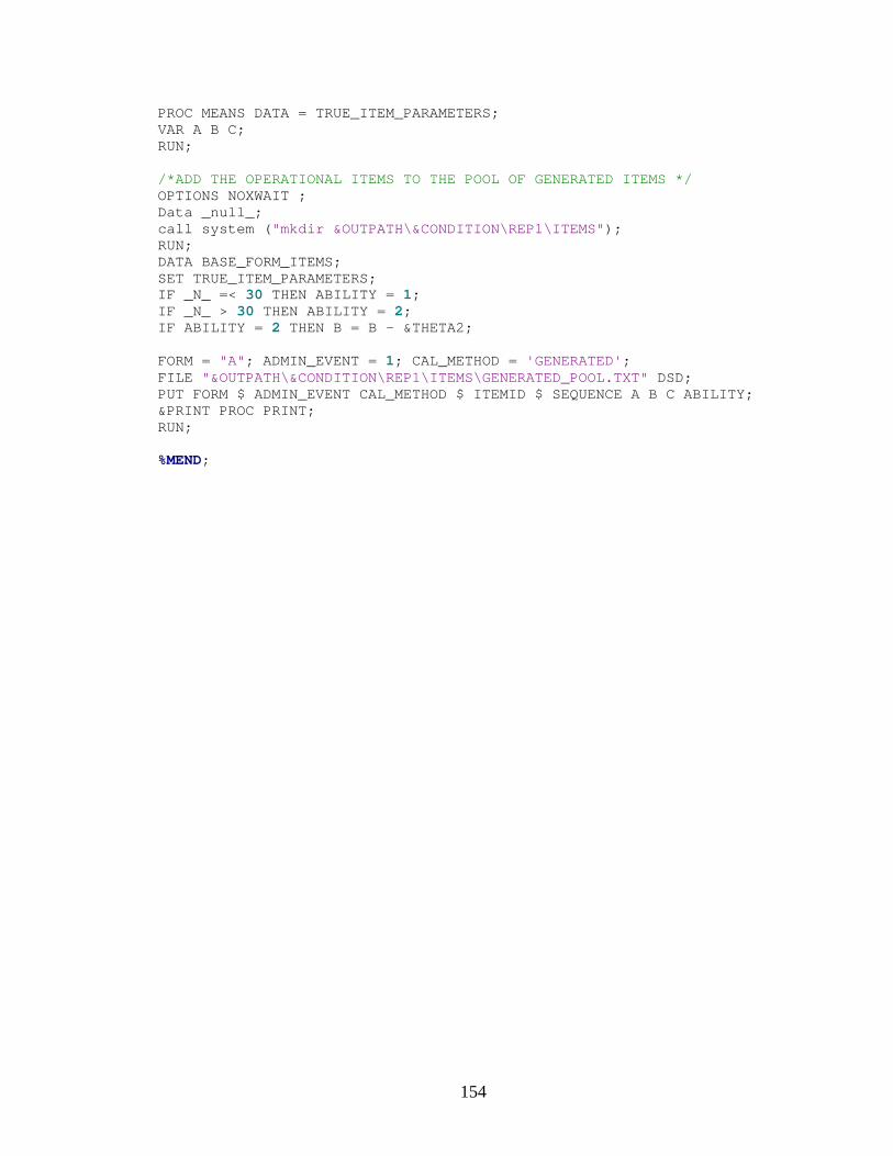
154

PROC MEANS DATA = TRUE_ITEM_PARAMETERS; VAR A B C; RUN; /*ADD THE OPERATIONAL ITEMS TO THE POOL OF GENERATED ITEMS */ OPTIONS NOXWAIT ; Data _null_; call system ("mkdir &OUTPATH\&CONDITION\REP1\ITEMS"); RUN; DATA BASE_FORM_ITEMS; SET TRUE_ITEM_PARAMETERS; IF _N_ =< 30 THEN ABILITY = 1; IF _N_ > 30 THEN ABILITY = 2; IF ABILITY = 2 THEN B = B - &THETA2; FORM = "A"; ADMIN_EVENT = 1; CAL_METHOD = 'GENERATED'; FILE "&OUTPATH\&CONDITION\REP1\ITEMS\GENERATED_POOL.TXT" DSD; PUT FORM $ ADMIN_EVENT CAL_METHOD $ ITEMID $ SEQUENCE A B C ABILITY; &PRINT PROC PRINT; RUN; %MEND;

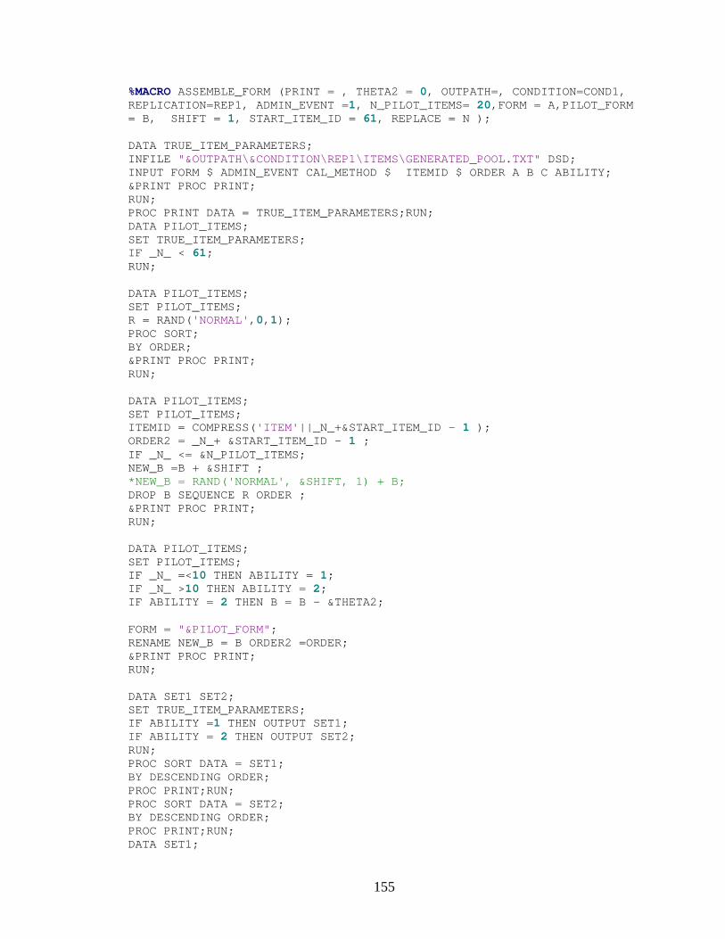
155

%MACRO ASSEMBLE_FORM (PRINT = , THETA2 = 0, OUTPATH=, CONDITION=COND1, REPLICATION=REP1, ADMIN_EVENT =1, N_PILOT_ITEMS= 20,FORM = A,PILOT_FORM = B, SHIFT = 1, START_ITEM_ID = 61, REPLACE = N ); DATA TRUE_ITEM_PARAMETERS; INFILE "&OUTPATH\&CONDITION\REP1\ITEMS\GENERATED_POOL.TXT" DSD; INPUT FORM $ ADMIN_EVENT CAL_METHOD $ ITEMID $ ORDER A B C ABILITY; &PRINT PROC PRINT; RUN; PROC PRINT DATA = TRUE_ITEM_PARAMETERS;RUN; DATA PILOT_ITEMS; SET TRUE_ITEM_PARAMETERS; IF _N_ < 61; RUN; DATA PILOT_ITEMS; SET PILOT_ITEMS; R = RAND('NORMAL',0,1); PROC SORT; BY ORDER; &PRINT PROC PRINT; RUN; DATA PILOT_ITEMS; SET PILOT_ITEMS; ITEMID = COMPRESS('ITEM'||_N_+&START_ITEM_ID - 1 ); ORDER2 = _N_+ &START_ITEM_ID - 1 ; IF _N_ <= &N_PILOT_ITEMS; NEW_B =B + &SHIFT ; *NEW_B = RAND('NORMAL', &SHIFT, 1) + B; DROP B SEQUENCE R ORDER ; &PRINT PROC PRINT; RUN; DATA PILOT_ITEMS; SET PILOT_ITEMS; IF _N_ =<10 THEN ABILITY = 1; IF _N_ >10 THEN ABILITY = 2; IF ABILITY = 2 THEN B = B - &THETA2; FORM = "&PILOT_FORM"; RENAME NEW_B = B ORDER2 =ORDER; &PRINT PROC PRINT; RUN; DATA SET1 SET2; SET TRUE_ITEM_PARAMETERS; IF ABILITY =1 THEN OUTPUT SET1; IF ABILITY = 2 THEN OUTPUT SET2; RUN; PROC SORT DATA = SET1; BY DESCENDING ORDER; PROC PRINT;RUN; PROC SORT DATA = SET2; BY DESCENDING ORDER; PROC PRINT;RUN; DATA SET1;

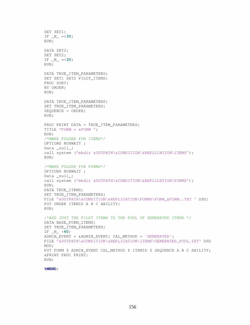
156

SET SET1; IF _N_ =<30; RUN; DATA SET2; SET SET2; IF _N_ =<30; RUN; DATA TRUE_ITEM_PARAMETERS; SET SET1 SET2 PILOT_ITEMS; PROC SORT; BY ORDER; RUN; DATA TRUE_ITEM_PARAMETERS; SET TRUE_ITEM_PARAMETERS; SEQUENCE = ORDER; RUN; PROC PRINT DATA = TRUE_ITEM_PARAMETERS; TITLE "FORM = &FORM "; RUN; /*MAKE FOLDER FOR ITEMS*/ OPTIONS NOXWAIT ; Data _null_; call system ("mkdir &OUTPATH\&CONDITION\&REPLICATION\ITEMS"); RUN; /*MAKE FOLDER FOR FORMS*/ OPTIONS NOXWAIT ; Data _null_; call system ("mkdir &OUTPATH\&CONDITION\&REPLICATION\FORMS"); RUN; DATA TRUE_ITEMS; SET TRUE_ITEM_PARAMETERS; FILE "&OUTPATH\&CONDITION\&REPLICATION\FORMS\FORM_&FORM..TXT " DSD; PUT ORDER ITEMID A B C ABILITY; RUN; /*ADD JUST THE PILOT ITEMS TO THE POOL OF GENERATED ITEMS */ DATA BASE_FORM_ITEMS; SET TRUE_ITEM_PARAMETERS; IF _N_ >60; ADMIN_EVENT = &ADMIN_EVENT; CAL_METHOD = 'GENERATED'; FILE "&OUTPATH\&CONDITION\&REPLICATION\ITEMS\GENERATED_POOL.TXT" DSD MOD; PUT FORM $ ADMIN_EVENT CAL_METHOD $ ITEMID $ SEQUENCE A B C ABILITY; &PRINT PROC PRINT; RUN; %MEND;

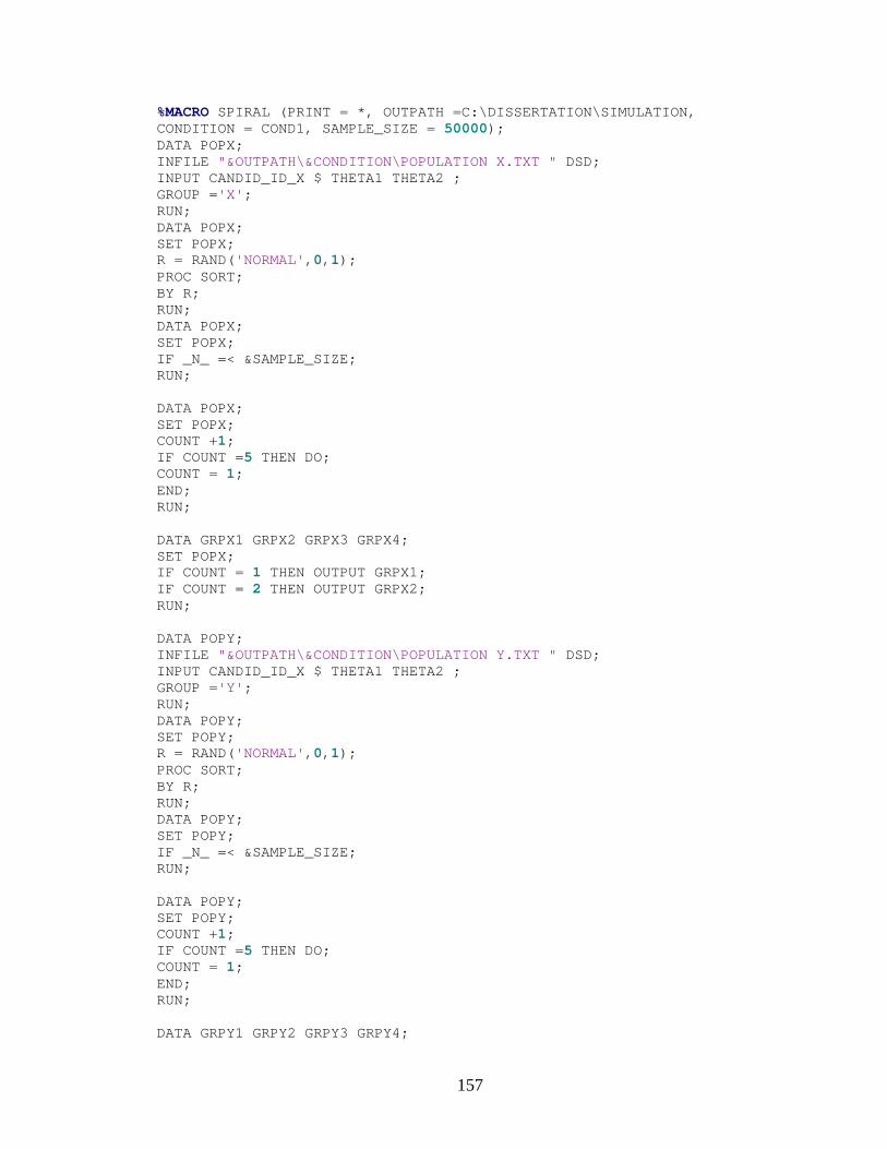
157

%MACRO SPIRAL (PRINT = *, OUTPATH =C:\DISSERTATION\SIMULATION, CONDITION = COND1, SAMPLE_SIZE = 50000); DATA POPX; INFILE "&OUTPATH\&CONDITION\POPULATION X.TXT " DSD; INPUT CANDID_ID_X $ THETA1 THETA2 ; GROUP ='X'; RUN; DATA POPX; SET POPX; R = RAND('NORMAL',0,1); PROC SORT; BY R; RUN; DATA POPX; SET POPX; IF _N_ =< &SAMPLE_SIZE; RUN; DATA POPX; SET POPX; COUNT +1; IF COUNT =5 THEN DO; COUNT = 1; END; RUN; DATA GRPX1 GRPX2 GRPX3 GRPX4; SET POPX; IF COUNT = 1 THEN OUTPUT GRPX1; IF COUNT = 2 THEN OUTPUT GRPX2; RUN; DATA POPY; INFILE "&OUTPATH\&CONDITION\POPULATION Y.TXT " DSD; INPUT CANDID_ID_X $ THETA1 THETA2 ; GROUP ='Y'; RUN; DATA POPY; SET POPY; R = RAND('NORMAL',0,1); PROC SORT; BY R; RUN; DATA POPY; SET POPY; IF _N_ =< &SAMPLE_SIZE; RUN; DATA POPY; SET POPY; COUNT +1; IF COUNT =5 THEN DO; COUNT = 1; END; RUN; DATA GRPY1 GRPY2 GRPY3 GRPY4;

158

SET POPY; IF COUNT = 1 THEN OUTPUT GRPY1; IF COUNT = 2 THEN OUTPUT GRPY2; RUN; DATA GRP1XY; SET GRPX1 GRPY1; PROC SORT; BY GROUP; RUN; DATA GRP2XY; SET GRPX2 GRPY2; PROC SORT; BY GROUP; RUN; DATA GRP1XY; SET GRP1XY; FILE "&OUTPATH\&CONDITION\GRP1XY.TXT " ; /*RETRIEVE FORM FROM FIRST REPLICATION*/ PUT CANDID_ID_X THETA1 THETA2 GROUP; RUN; DATA GRP2XY; SET GRP2XY; FILE "&OUTPATH\&CONDITION\GRP2XY.TXT " ; /*RETRIEVE FORM FROM FIRST REPLICATION*/ PUT CANDID_ID_X THETA1 THETA2 GROUP; RUN; PROC MEANS DATA = GRP1XY; VAR THETA1 THETA2; OUTPUT OUT = MN_GRP1XY; RUN; DATA MN_GRP1XY; SET MN_GRP1XY; FILE "&OUTPATH\&CONDITION\MOMENTS_GRP1XY.TXT " ; PUT _STAT_ THETA1 THETA2; RUN; PROC MEANS DATA = GRP2XY; VAR THETA1 THETA2; OUTPUT OUT = MN_GRP2XY; RUN; DATA MN_GRP2XY; SET MN_GRP2XY; FILE "&OUTPATH\&CONDITION\MOMENTS_GRP2XY.TXT " ; PUT _STAT_ THETA1 THETA2; RUN; %MEND;

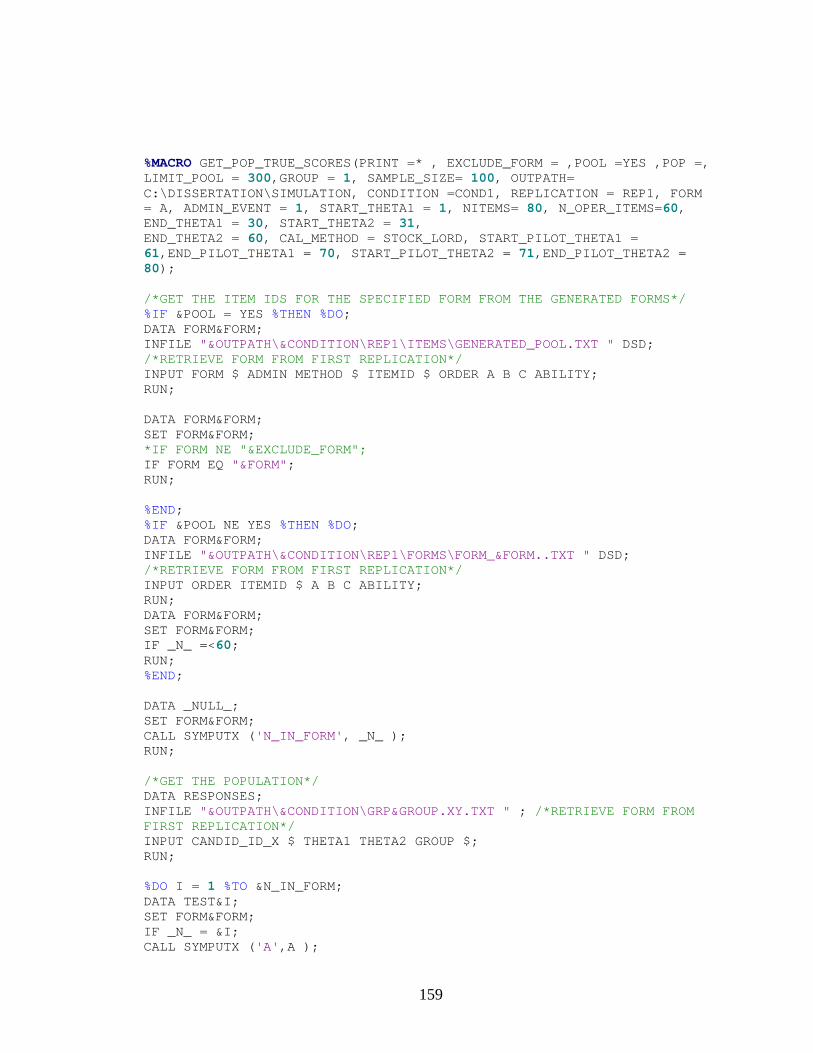
159

%MACRO GET_POP_TRUE_SCORES(PRINT =* , EXCLUDE_FORM = ,POOL =YES ,POP =, LIMIT_POOL = 300,GROUP = 1, SAMPLE_SIZE= 100, OUTPATH= C:\DISSERTATION\SIMULATION, CONDITION =COND1, REPLICATION = REP1, FORM = A, ADMIN_EVENT = 1, START_THETA1 = 1, NITEMS= 80, N_OPER_ITEMS=60, END_THETA1 = 30, START_THETA2 = 31, END_THETA2 = 60, CAL_METHOD = STOCK_LORD, START_PILOT_THETA1 = 61,END_PILOT_THETA1 = 70, START_PILOT_THETA2 = 71,END_PILOT_THETA2 = 80); /*GET THE ITEM IDS FOR THE SPECIFIED FORM FROM THE GENERATED FORMS*/ %IF &POOL = YES %THEN %DO; DATA FORM&FORM; INFILE "&OUTPATH\&CONDITION\REP1\ITEMS\GENERATED_POOL.TXT " DSD; /*RETRIEVE FORM FROM FIRST REPLICATION*/ INPUT FORM $ ADMIN METHOD $ ITEMID $ ORDER A B C ABILITY; RUN; DATA FORM&FORM; SET FORM&FORM; *IF FORM NE "&EXCLUDE_FORM"; IF FORM EQ "&FORM"; RUN; %END; %IF &POOL NE YES %THEN %DO; DATA FORM&FORM; INFILE "&OUTPATH\&CONDITION\REP1\FORMS\FORM_&FORM..TXT " DSD; /*RETRIEVE FORM FROM FIRST REPLICATION*/ INPUT ORDER ITEMID $ A B C ABILITY; RUN; DATA FORM&FORM; SET FORM&FORM; IF _N_ =<60; RUN; %END; DATA _NULL_; SET FORM&FORM; CALL SYMPUTX ('N_IN_FORM', _N_ ); RUN; /*GET THE POPULATION*/ DATA RESPONSES; INFILE "&OUTPATH\&CONDITION\GRP&GROUP.XY.TXT " ; /*RETRIEVE FORM FROM FIRST REPLICATION*/ INPUT CANDID_ID_X $ THETA1 THETA2 GROUP $; RUN; %DO I = 1 %TO &N_IN_FORM; DATA TEST&I; SET FORM&FORM; IF _N_ = &I; CALL SYMPUTX ('A',A );

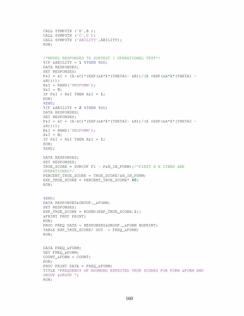
160

CALL SYMPUTX ('B',B ); CALL SYMPUTX ('C',C ); CALL SYMPUTX ('ABILITY',ABILITY); RUN; /*MODEL RESPONSES TO SUBTEST 1 OPERATIONAL TEST*/ %IF &ABILITY = 1 %THEN %DO; DATA RESPONSES; SET RESPONSES; P&I = &C + (1-&C)*(EXP(&A*1*(THETA1- &B))/(1 +EXP(&A*1*(THETA1 - &B)))); R&I = RAND('UNIFORM'); X&I = 0; IF P&I > R&I THEN X&I = 1; RUN; %END; %IF &ABILITY = 2 %THEN %DO; DATA RESPONSES; SET RESPONSES; P&I = &C + (1-&C)*(EXP(&A*1*(THETA2- &B))/(1 +EXP(&A*1*(THETA2 - &B)))); R&I = RAND('UNIFORM'); X&I = 0; IF P&I > R&I THEN X&I = 1; RUN; %END; DATA RESPONSES; SET RESPONSES; TRUE_SCORE = SUM(OF P1 - P&N_IN_FORM);/*FIRST X N ITEMS ARE OPERATIONAL*/ PERCENT_TRUE_SCORE = TRUE_SCORE/&N_IN_FORM; EXP_TRUE_SCORE = PERCENT_TRUE_SCORE* 60; RUN; %END; DATA RESPONSES&GROUP._&FORM; SET RESPONSES; EXP_TRUE_SCORE = ROUND(EXP_TRUE_SCORE,1); &PRINT PROC PRINT; RUN; PROC FREQ DATA = RESPONSES&GROUP._&FORM NOPRINT; TABLE EXP_TRUE_SCORE/ OUT = FREQ_&FORM; RUN; DATA FREQ_&FORM; SET FREQ_&FORM; COUNT_&FORM = COUNT; RUN; PROC PRINT DATA = FREQ_&FORM; TITLE "FREQUENCY OF ROUNDED EXPECTED TRUE SCORES FOR FORM &FORM AND GROUP &GROUP "; RUN;

161

DATA FREQ_&FORM; SET FREQ_&FORM; N_ITEMS =&N_IN_FORM ; FILE "&OUTPATH\&CONDITION\FREQ_&FORM..TXT " DSD; PUT EXP_TRUE_SCORE COUNT_&FORM PERCENT N_ITEMS; RUN; %MEND;

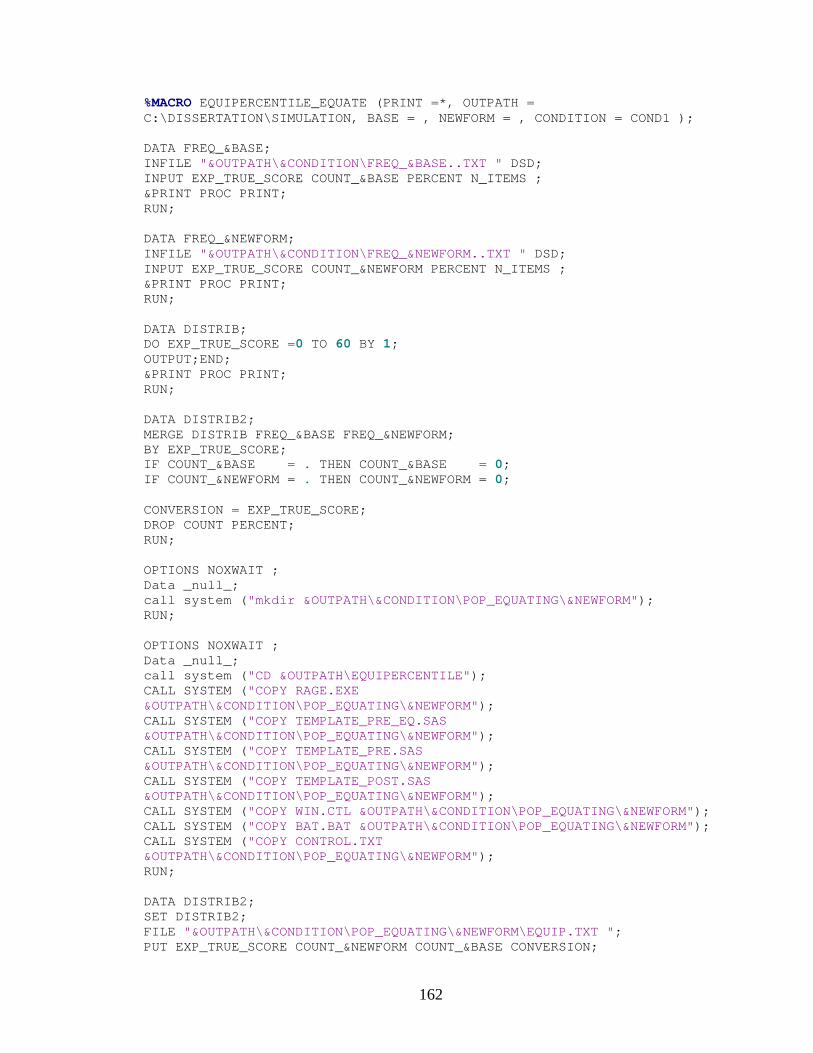
162

%MACRO EQUIPERCENTILE_EQUATE (PRINT =*, OUTPATH = C:\DISSERTATION\SIMULATION, BASE = , NEWFORM = , CONDITION = COND1 ); DATA FREQ_&BASE; INFILE "&OUTPATH\&CONDITION\FREQ_&BASE..TXT " DSD; INPUT EXP_TRUE_SCORE COUNT_&BASE PERCENT N_ITEMS ; &PRINT PROC PRINT; RUN; DATA FREQ_&NEWFORM; INFILE "&OUTPATH\&CONDITION\FREQ_&NEWFORM..TXT " DSD; INPUT EXP_TRUE_SCORE COUNT_&NEWFORM PERCENT N_ITEMS ; &PRINT PROC PRINT; RUN; DATA DISTRIB; DO EXP_TRUE_SCORE =0 TO 60 BY 1; OUTPUT;END; &PRINT PROC PRINT; RUN; DATA DISTRIB2; MERGE DISTRIB FREQ_&BASE FREQ_&NEWFORM; BY EXP_TRUE_SCORE; IF COUNT_&BASE = . THEN COUNT_&BASE = 0; IF COUNT_&NEWFORM = . THEN COUNT_&NEWFORM = 0; CONVERSION = EXP_TRUE_SCORE; DROP COUNT PERCENT; RUN; OPTIONS NOXWAIT ; Data _null_; call system ("mkdir &OUTPATH\&CONDITION\POP_EQUATING\&NEWFORM"); RUN; OPTIONS NOXWAIT ; Data _null_; call system ("CD &OUTPATH\EQUIPERCENTILE"); CALL SYSTEM ("COPY RAGE.EXE &OUTPATH\&CONDITION\POP_EQUATING\&NEWFORM"); CALL SYSTEM ("COPY TEMPLATE_PRE_EQ.SAS &OUTPATH\&CONDITION\POP_EQUATING\&NEWFORM"); CALL SYSTEM ("COPY TEMPLATE_PRE.SAS &OUTPATH\&CONDITION\POP_EQUATING\&NEWFORM"); CALL SYSTEM ("COPY TEMPLATE_POST.SAS &OUTPATH\&CONDITION\POP_EQUATING\&NEWFORM"); CALL SYSTEM ("COPY WIN.CTL &OUTPATH\&CONDITION\POP_EQUATING\&NEWFORM"); CALL SYSTEM ("COPY BAT.BAT &OUTPATH\&CONDITION\POP_EQUATING\&NEWFORM"); CALL SYSTEM ("COPY CONTROL.TXT &OUTPATH\&CONDITION\POP_EQUATING\&NEWFORM"); RUN; DATA DISTRIB2; SET DISTRIB2; FILE "&OUTPATH\&CONDITION\POP_EQUATING\&NEWFORM\EQUIP.TXT "; PUT EXP_TRUE_SCORE COUNT_&NEWFORM COUNT_&BASE CONVERSION;

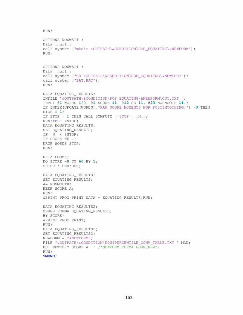
163

RUN; OPTIONS NOXWAIT ; Data _null_; call system ("mkdir &OUTPATH\&CONDITION\POP_EQUATING\&NEWFORM"); RUN; OPTIONS NOXWAIT ; Data _null_; call system ("CD &OUTPATH\&CONDITION\POP_EQUATING\&NEWFORM"); call system ("BAT.BAT"); RUN; DATA EQUATING_RESULTS; INFILE "&OUTPATH\&CONDITION\POP_EQUATING\&NEWFORM\OUT.TXT "; INPUT @1 WORDS $80. @1 SCORE 11. @12 SE 11. @23 NOSMOOTH 11.; IF INDEX(UPCASE(WORDS),"RAW SCORE MOMENTS FOR POSTSMOOTHING:") >0 THEN STOP = 1; IF STOP = 1 THEN CALL SYMPUTX ('STOP', _N_); RUN;%PUT &STOP; DATA EQUATING_RESULTS; SET EQUATING_RESULTS; IF _N_ < &STOP; IF SCORE NE .; DROP WORDS STOP; RUN; DATA FORMA; DO SCORE =0 TO 60 BY 1; OUTPUT; END;RUN; DATA EQUATING_RESULTS; SET EQUATING_RESULTS; A= NOSMOOTH; KEEP SCORE A; RUN; &PRINT PROC PRINT DATA = EQUATING_RESULTS;RUN; DATA EQUATING_RESULTS2; MERGE FORMA EQUATING_RESULTS; BY SCORE; &PRINT PROC PRINT; RUN; DATA EQUATING_RESULTS2; SET EQUATING_RESULTS2; NEWFORM = "&NEWFORM"; FILE "&OUTPATH\&CONDITION\EQUIPERCENTILE_CONV_TABLE.TXT " MOD; PUT NEWFORM SCORE A ; /*NEWFORM FORMA FORM_NEW*/ RUN; %MEND;

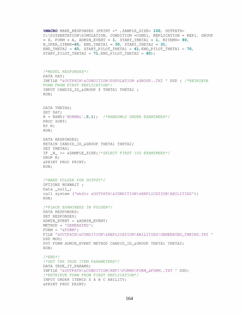
164

%MACRO MAKE_RESPONSES (PRINT =* ,SAMPLE_SIZE= 100, OUTPATH= C:\DISSERTATION\SIMULATION, CONDITION =COND1, REPLICATION = REP1, GROUP = X, FORM = A, ADMIN_EVENT = 1, START_THETA1 = 1, NITEMS= 80, N_OPER_ITEMS=60, END_THETA1 = 30, START_THETA2 = 31, END_THETA2 = 60, START_PILOT_THETA1 = 61,END_PILOT_THETA1 = 70, START_PILOT_THETA2 = 71,END_PILOT_THETA2 = 80); /*MODEL RESPONSES*/ DATA DAT; INFILE "&OUTPATH\&CONDITION\POPULATION &GROUP..TXT " DSD ; /*RETRIEVE FORM FROM FIRST REPLICATION*/ INPUT CANDID_ID_&GROUP $ THETA1 THETA2 ; RUN; DATA THETAS; SET DAT; R = RAND('NORMAL',0,1); /*RANDOMLY ORDER EXAMINEES*/ PROC SORT; BY R; RUN; DATA RESPONSES; RETAIN CANDID_ID_&GROUP THETA1 THETA2; SET THETAS; IF _N_ <= &SAMPLE_SIZE;/*SELECT FIRST 100 EXAMINEES*/ DROP R; &PRINT PROC PRINT; RUN; /*MAKE FOLDER FOR OUTPUT*/ OPTIONS NOXWAIT ; Data _null_; call system ("mkdir &OUTPATH\&CONDITION\&REPLICATION\ABILITIES"); RUN; /*PLACE EXAMINEES IN FOLDER*/ DATA RESPONSES; SET RESPONSES; ADMIN_EVENT = &ADMIN_EVENT; METHOD = "GENERATED"; FORM = "&FORM"; FILE "&OUTPATH\&CONDITION\&REPLICATION\ABILITIES\GENERATED_THETAS.TXT " DSD MOD; PUT FORM ADMIN_EVENT METHOD CANDID_ID_&GROUP THETA1 THETA2; RUN; /*END*/ /*GET THE TRUE ITEM PARAMETERS*/ DATA TRUE_IT_PARAMS; INFILE "&OUTPATH\&CONDITION\REP1\FORMS\FORM_&FORM..TXT " DSD; /*RETRIEVE FORM FROM FIRST REPLICATION*/ INPUT ORDER ITEMID $ A B C ABILITY; &PRINT PROC PRINT;

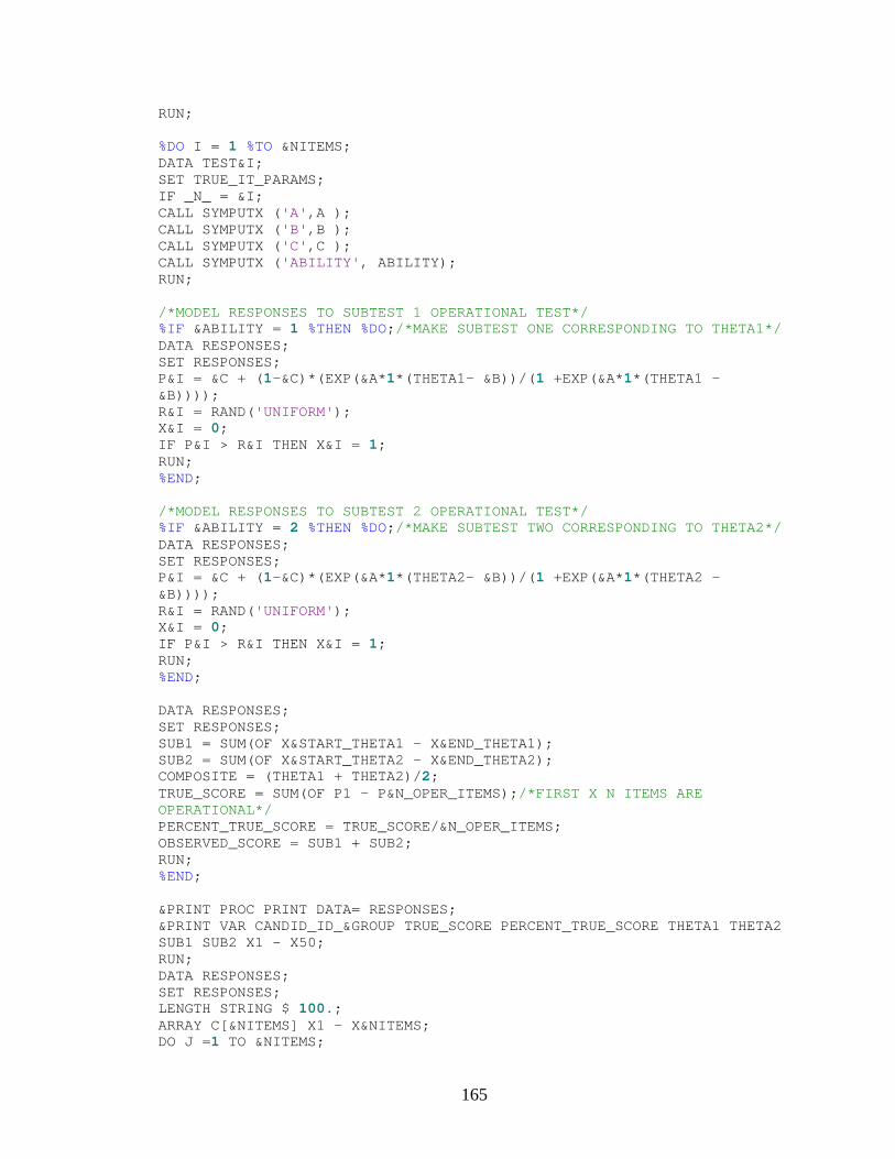
165

RUN; %DO I = 1 %TO &NITEMS; DATA TEST&I; SET TRUE_IT_PARAMS; IF _N_ = &I; CALL SYMPUTX ('A',A ); CALL SYMPUTX ('B',B ); CALL SYMPUTX ('C',C ); CALL SYMPUTX ('ABILITY', ABILITY); RUN; /*MODEL RESPONSES TO SUBTEST 1 OPERATIONAL TEST*/ %IF &ABILITY = 1 %THEN %DO;/*MAKE SUBTEST ONE CORRESPONDING TO THETA1*/ DATA RESPONSES; SET RESPONSES; P&I = &C + (1-&C)*(EXP(&A*1*(THETA1- &B))/(1 +EXP(&A*1*(THETA1 - &B)))); R&I = RAND('UNIFORM'); X&I = 0; IF P&I > R&I THEN X&I = 1; RUN; %END; /*MODEL RESPONSES TO SUBTEST 2 OPERATIONAL TEST*/ %IF &ABILITY = 2 %THEN %DO;/*MAKE SUBTEST TWO CORRESPONDING TO THETA2*/ DATA RESPONSES; SET RESPONSES; P&I = &C + (1-&C)*(EXP(&A*1*(THETA2- &B))/(1 +EXP(&A*1*(THETA2 - &B)))); R&I = RAND('UNIFORM'); X&I = 0; IF P&I > R&I THEN X&I = 1; RUN; %END; DATA RESPONSES; SET RESPONSES; SUB1 = SUM(OF X&START_THETA1 - X&END_THETA1); SUB2 = SUM(OF X&START_THETA2 - X&END_THETA2); COMPOSITE = (THETA1 + THETA2)/2; TRUE_SCORE = SUM(OF P1 - P&N_OPER_ITEMS);/*FIRST X N ITEMS ARE OPERATIONAL*/ PERCENT_TRUE_SCORE = TRUE_SCORE/&N_OPER_ITEMS; OBSERVED_SCORE = SUB1 + SUB2; RUN; %END; &PRINT PROC PRINT DATA= RESPONSES; &PRINT VAR CANDID_ID_&GROUP TRUE_SCORE PERCENT_TRUE_SCORE THETA1 THETA2 SUB1 SUB2 X1 - X50; RUN; DATA RESPONSES; SET RESPONSES; LENGTH STRING $ 100.; ARRAY C[&NITEMS] X1 - X&NITEMS; DO J =1 TO &NITEMS;

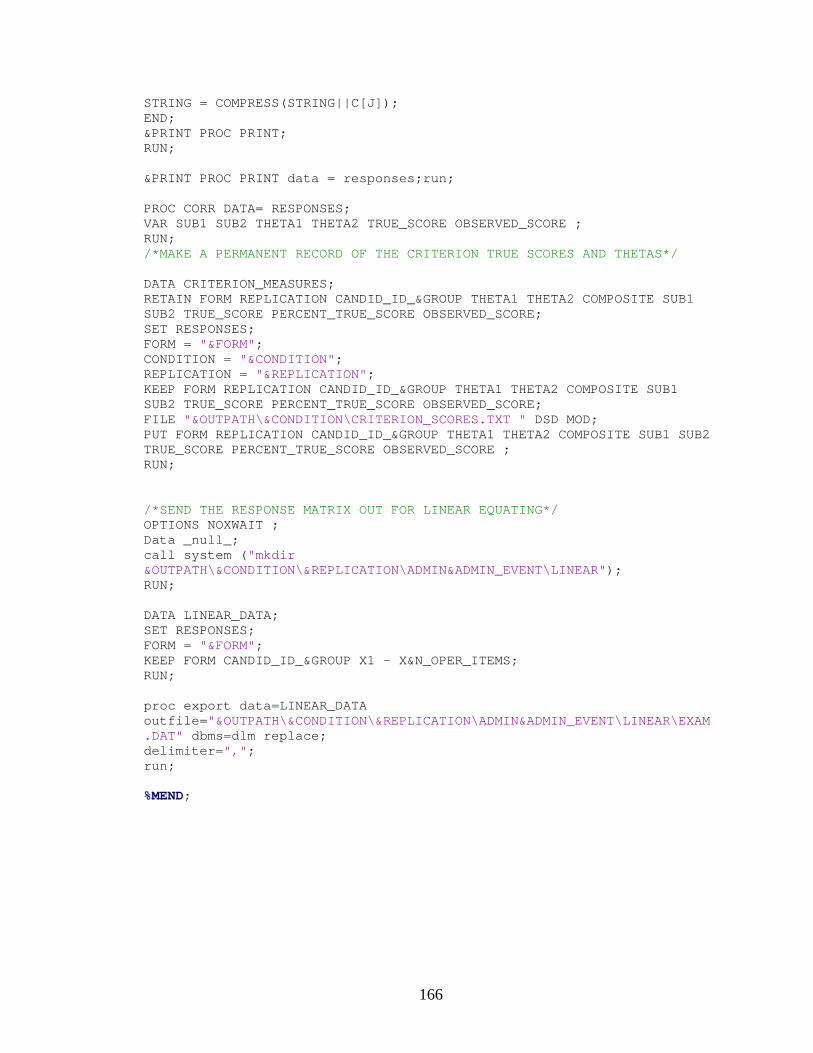
166

STRING = COMPRESS(STRING||C[J]); END; &PRINT PROC PRINT; RUN; &PRINT PROC PRINT data = responses;run; PROC CORR DATA= RESPONSES; VAR SUB1 SUB2 THETA1 THETA2 TRUE_SCORE OBSERVED_SCORE ; RUN; /*MAKE A PERMANENT RECORD OF THE CRITERION TRUE SCORES AND THETAS*/ DATA CRITERION_MEASURES; RETAIN FORM REPLICATION CANDID_ID_&GROUP THETA1 THETA2 COMPOSITE SUB1 SUB2 TRUE_SCORE PERCENT_TRUE_SCORE OBSERVED_SCORE; SET RESPONSES; FORM = "&FORM"; CONDITION = "&CONDITION"; REPLICATION = "&REPLICATION"; KEEP FORM REPLICATION CANDID_ID_&GROUP THETA1 THETA2 COMPOSITE SUB1 SUB2 TRUE_SCORE PERCENT_TRUE_SCORE OBSERVED_SCORE; FILE "&OUTPATH\&CONDITION\CRITERION_SCORES.TXT " DSD MOD; PUT FORM REPLICATION CANDID_ID_&GROUP THETA1 THETA2 COMPOSITE SUB1 SUB2 TRUE_SCORE PERCENT_TRUE_SCORE OBSERVED_SCORE ; RUN; /*SEND THE RESPONSE MATRIX OUT FOR LINEAR EQUATING*/ OPTIONS NOXWAIT ; Data _null_; call system ("mkdir &OUTPATH\&CONDITION\&REPLICATION\ADMIN&ADMIN_EVENT\LINEAR"); RUN; DATA LINEAR_DATA; SET RESPONSES; FORM = "&FORM"; KEEP FORM CANDID_ID_&GROUP X1 - X&N_OPER_ITEMS; RUN; proc export data=LINEAR_DATA outfile="&OUTPATH\&CONDITION\&REPLICATION\ADMIN&ADMIN_EVENT\LINEAR\EXAM.DAT" dbms=dlm replace; delimiter=","; run; %MEND;

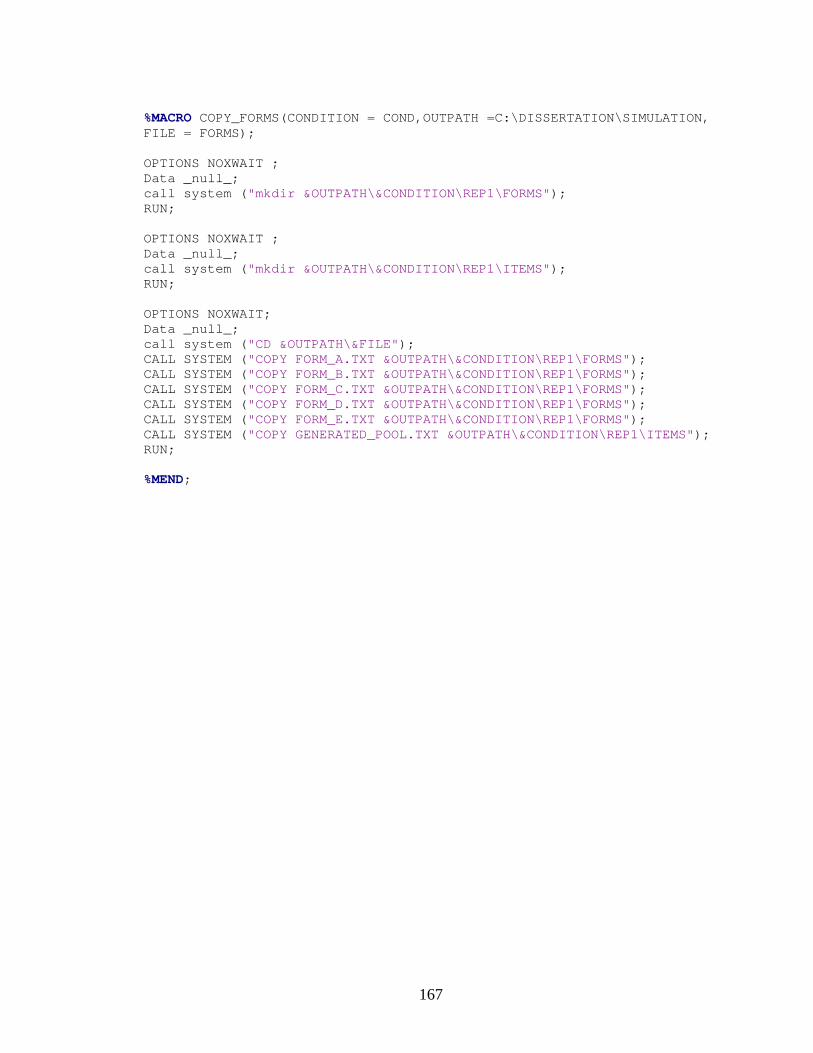
167

%MACRO COPY_FORMS(CONDITION = COND,OUTPATH =C:\DISSERTATION\SIMULATION, FILE = FORMS); OPTIONS NOXWAIT ; Data _null_; call system ("mkdir &OUTPATH\&CONDITION\REP1\FORMS"); RUN; OPTIONS NOXWAIT ; Data _null_; call system ("mkdir &OUTPATH\&CONDITION\REP1\ITEMS"); RUN; OPTIONS NOXWAIT; Data _null_; call system ("CD &OUTPATH\&FILE"); CALL SYSTEM ("COPY FORM_A.TXT &OUTPATH\&CONDITION\REP1\FORMS"); CALL SYSTEM ("COPY FORM_B.TXT &OUTPATH\&CONDITION\REP1\FORMS"); CALL SYSTEM ("COPY FORM_C.TXT &OUTPATH\&CONDITION\REP1\FORMS"); CALL SYSTEM ("COPY FORM_D.TXT &OUTPATH\&CONDITION\REP1\FORMS"); CALL SYSTEM ("COPY FORM_E.TXT &OUTPATH\&CONDITION\REP1\FORMS"); CALL SYSTEM ("COPY GENERATED_POOL.TXT &OUTPATH\&CONDITION\REP1\ITEMS"); RUN; %MEND;

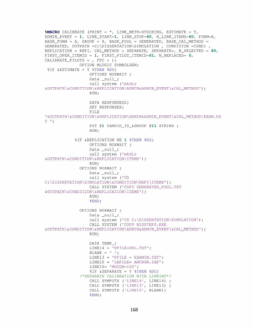
168

%MACRO CALIBRATE (PRINT = *, LINK_METH=STOCKING, ESTIMATE = Y, ADMIN_EVENT = 1, LINK_START=1, LINK_STOP=60, N_LINK_ITEMS=60, FORM=A, BASE_FORM = A, GROUP = X, BASE_POOL = GENERATED, BASE_CAL_METHOD = GENERATED, OUTPATH =C:\DISSERTATION\SIMULATION , CONDITION =COND1 , REPLICATION = REP1, CAL_METHOD = SEPARATE, SEPARATE=, N_SELECTED = 80, FIRST_OPER_ITEMID = 1, FIRST_PILOT_ITEMID=61, N_REPLACED= 0, CALIBRATE_PILOTS = , FPC = ); OPTION MLOGIC SYMBOLGEN; %IF &ESTIMATE = Y %THEN %DO; OPTIONS NOXWAIT ; Data _null_; call system ("mkdir &OUTPATH\&CONDITION\&REPLICATION\ADMIN&ADMIN_EVENT\&CAL_METHOD"); RUN; DATA RESPONSES2; SET RESPONSES; FILE "&OUTPATH\&CONDITION\&REPLICATION\ADMIN&ADMIN_EVENT\&CAL_METHOD\EXAM.DAT "; PUT @1 CANDID_ID_&GROUP @11 STRING ; RUN; %IF &REPLICATION NE 1 %THEN %DO; OPTIONS NOXWAIT ; Data _null_; call system ("mkdir &OUTPATH\&CONDITION\&REPLICATION\ITEMS"); RUN; OPTIONS NOXWAIT ; Data _null_; call system ("CD C:\DISSERTATION\SIMULATION\&CONDITION\REP1\ITEMS"); CALL SYSTEM ("COPY GENERATED_POOL.TXT &OUTPATH\&CONDITION\&REPLICATION\ITEMS"); RUN; %END; OPTIONS NOXWAIT ; Data _null_; call system ("CD C:\DISSERTATION\SIMULATION"); CALL SYSTEM ("COPY BIGSTEPS.EXE &OUTPATH\&CONDITION\&REPLICATION\ADMIN&ADMIN_EVENT\&CAL_METHOD"); RUN; DATA TEMP_; LINE14 = "DFILE=DEL.TXT"; BLANK = " "; LINE13 = "PFILE = EXAMIN.TXT"; LINE10 = "IAFILE= ANCHOR.IAF"; LINE15= "MUCON=100"; %IF &SEPARATE = Y %THEN %DO; /*SEPARATE CALIBRATION WITH LINKING*/ CALL SYMPUTX ('LINE14', LINE14) ; CALL SYMPUTX ('LINE13', LINE13) ; CALL SYMPUTX ('LINE10', BLANK); %END;

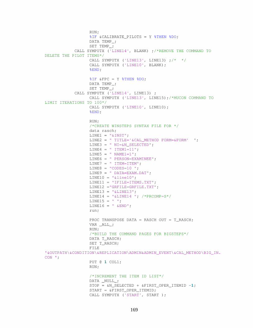
169

RUN; %IF &CALIBRATE_PILOTS = Y %THEN %DO; DATA TEMP_; SET TEMP_; CALL SYMPUTX ('LINE14', BLANK) ;/*REMOVE THE COMMAND TO DELETE THE PILOT ITEMS*/ CALL SYMPUTX ('LINE13', LINE13) ;/* */ CALL SYMPUTX ('LINE10', BLANK); %END; %IF &FPC = Y %THEN %DO; DATA TEMP_; SET TEMP_; CALL SYMPUTX ('LINE14', LINE13) ; CALL SYMPUTX ('LINE13', LINE15);/*MUCON COMMAND TO LIMIT ITERATIONS TO 100*/ CALL SYMPUTX ('LINE10', LINE10); %END; RUN; /*CREATE WINSTEPS SYNTAX FILE FOR */ data rasch; LINE1 = "&INST"; LINE2 = " TITLE='&CAL_METHOD FORM=&FORM' "; LINE3 = " NI=&N_SELECTED"; LINE4 = " ITEM1=11"; LINE5 = " NAME1=1"; LINE6 = " PERSON=EXAMINEE"; LINE7 = " ITEM=ITEM"; LINE8 = "CODES=10 "; LINE9 = " DATA=EXAM.DAT"; LINE10 = "&line10"; LINE11 = "IFILE=ITEMS.TXT"; LINE12 ="GRFILE=GRFILE.TXT"; LINE13 = "&LINE13"; LINE14 = "&LINE14 "; /*PRCOMP=S*/ LINE15 = " "; LINE16 = " &END"; run; PROC TRANSPOSE DATA = RASCH OUT = T_RASCH; VAR _ALL_; RUN; /*BUILD THE COMMAND PAGES FOR BIGSTEPS*/ DATA T_RASCH; SET T_RASCH; FILE "&OUTPATH\&CONDITION\&REPLICATION\ADMIN&ADMIN_EVENT\&CAL_METHOD\BIG_IN.CON "; PUT @ 1 COL1; RUN; /*INCREMENT THE ITEM ID LIST*/ DATA _NULL_; STOP = &N_SELECTED + &FIRST_OPER_ITEMID -1; START = &FIRST_OPER_ITEMID; CALL SYMPUTX ('START', START );

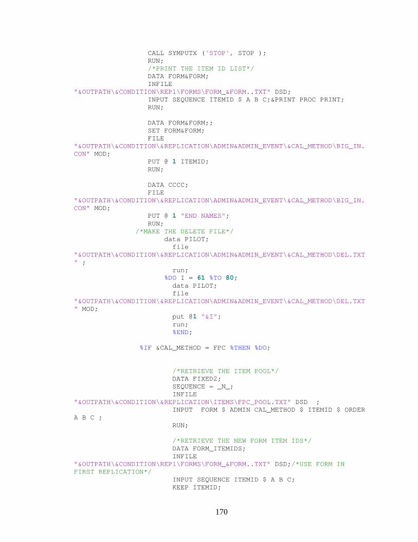
170

CALL SYMPUTX ('STOP', STOP ); RUN; /*PRINT THE ITEM ID LIST*/ DATA FORM&FORM; INFILE "&OUTPATH\&CONDITION\REP1\FORMS\FORM_&FORM..TXT" DSD; INPUT SEQUENCE ITEMID $ A B C;&PRINT PROC PRINT; RUN; DATA FORM&FORM;; SET FORM&FORM; FILE "&OUTPATH\&CONDITION\&REPLICATION\ADMIN&ADMIN_EVENT\&CAL_METHOD\BIG_IN.CON" MOD; PUT @ 1 ITEMID; RUN; DATA CCCC; FILE "&OUTPATH\&CONDITION\&REPLICATION\ADMIN&ADMIN_EVENT\&CAL_METHOD\BIG_IN.CON" MOD; PUT @ 1 "END NAMES"; RUN; /*MAKE THE DELETE FILE*/ data PILOT; file "&OUTPATH\&CONDITION\&REPLICATION\ADMIN&ADMIN_EVENT\&CAL_METHOD\DEL.TXT" ; run; %DO I = 61 %TO 80; data PILOT; file "&OUTPATH\&CONDITION\&REPLICATION\ADMIN&ADMIN_EVENT\&CAL_METHOD\DEL.TXT" MOD; put @1 "&I"; run; %END; %IF &CAL_METHOD = FPC %THEN %DO; /*RETRIEVE THE ITEM POOL*/ DATA FIXED2; SEQUENCE = _N_; INFILE "&OUTPATH\&CONDITION\&REPLICATION\ITEMS\FPC_POOL.TXT" DSD ; INPUT FORM $ ADMIN CAL_METHOD $ ITEMID $ ORDER A B C ; RUN; /*RETRIEVE THE NEW FORM ITEM IDS*/ DATA FORM_ITEMIDS; INFILE "&OUTPATH\&CONDITION\REP1\FORMS\FORM_&FORM..TXT" DSD;/*USE FORM IN FIRST REPLICATION*/ INPUT SEQUENCE ITEMID $ A B C; KEEP ITEMID;

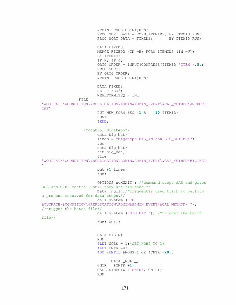
171

&PRINT PROC PRINT;RUN; PROC SORT DATA = FORM_ITEMIDS; BY ITEMID;RUN; PROC SORT DATA = FIXED2; BY ITEMID;RUN; DATA FIXED3; MERGE FIXED2 (IN =H) FORM_ITEMIDS (IN =J); BY ITEMID; IF H; IF J; ORIG_ORDER = INPUT(COMPRESS(ITEMID,'ITEM'),8.); PROC SORT; BY ORIG_ORDER; &PRINT PROC PRINT;RUN; DATA FIXED3; SET FIXED3; NEW_FORM_SEQ = _N_; FILE "&OUTPATH\&CONDITION\&REPLICATION\ADMIN&ADMIN_EVENT\&CAL_METHOD\ANCHOR.IAF"; PUT NEW_FORM_SEQ +1 B +10 ITEMID; RUN; %END; /*control Bigsteps*/ data big_bat; lines = "bigsteps BIG_IN.con BIG_OUT.txt"; run; data big_bat; set big_bat; file "&OUTPATH\&CONDITION\&REPLICATION\ADMIN&ADMIN_EVENT\&CAL_METHOD\BIG.BAT "; put @1 lines; run; OPTIONS noXWAIT ; /*command stops SAS and gives DOS and CIPE control until they are finished.*/ Data _null_;/*frequently used trick to perform a process reserved for data steps.*/ call system ("CD &OUTPATH\&CONDITION\&REPLICATION\ADMIN&ADMIN_EVENT\&CAL_METHOD\ "); /*trigger the batch file*/ call system ("BIG.BAT "); /*trigger the batch file*/ run; QUIT; DATA BIGIN; RUN; %LET NOBS = 1;*SET NOBS TO 1; %LET CNTR =0; %DO %UNTIL(&NOBS>1 OR &CNTR =20); DATA _NULL_; CNTR = &CNTR +1; CALL SYMPUTX ('CNTR', CNTR); RUN;

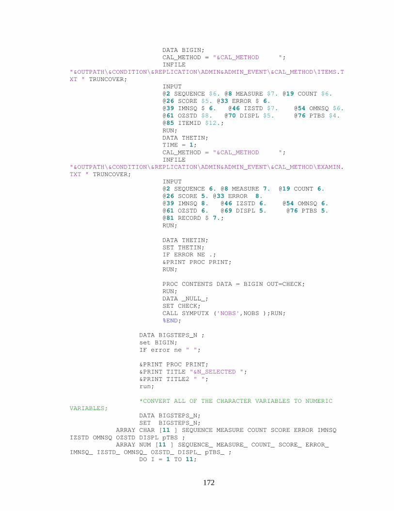
172

DATA BIGIN; CAL_METHOD = "&CAL_METHOD "; INFILE "&OUTPATH\&CONDITION\&REPLICATION\ADMIN&ADMIN_EVENT\&CAL_METHOD\ITEMS.TXT " TRUNCOVER; INPUT @2 SEQUENCE $6. @8 MEASURE $7. @19 COUNT $6. @26 SCORE $5. @33 ERROR $ 6. @39 IMNSQ $ 6. @46 IZSTD $7. @54 OMNSQ $6. @61 OZSTD $8. @70 DISPL $5. @76 PTBS $4. @85 ITEMID $12.; RUN; DATA THETIN; TIME = 1; CAL_METHOD = "&CAL_METHOD "; INFILE "&OUTPATH\&CONDITION\&REPLICATION\ADMIN&ADMIN_EVENT\&CAL_METHOD\EXAMIN.TXT " TRUNCOVER; INPUT @2 SEQUENCE 6. @8 MEASURE 7. @19 COUNT 6. @26 SCORE 5. @33 ERROR 8. @39 IMNSQ 8. @46 IZSTD 6. @54 OMNSQ 6. @61 OZSTD 6. @69 DISPL 5. @76 PTBS 5. @81 RECORD $ 7.; RUN; DATA THETIN; SET THETIN; IF ERROR NE .; &PRINT PROC PRINT; RUN; PROC CONTENTS DATA = BIGIN OUT=CHECK; RUN; DATA _NULL_; SET CHECK; CALL SYMPUTX ('NOBS',NOBS );RUN; %END; DATA BIGSTEPS_N ; set BIGIN; IF error ne " "; &PRINT PROC PRINT; &PRINT TITLE "&N_SELECTED "; &PRINT TITLE2 " "; run; *CONVERT ALL OF THE CHARACTER VARIABLES TO NUMERIC VARIABLES; DATA BIGSTEPS_N; SET BIGSTEPS_N; ARRAY CHAR [11 ] SEQUENCE MEASURE COUNT SCORE ERROR IMNSQ IZSTD OMNSQ OZSTD DISPL pTBS ; ARRAY NUM [11 ] SEQUENCE_ MEASURE_ COUNT_ SCORE_ ERROR_ IMNSQ_ IZSTD_ OMNSQ_ OZSTD_ DISPL_ pTBS_ ; DO I = 1 TO 11;

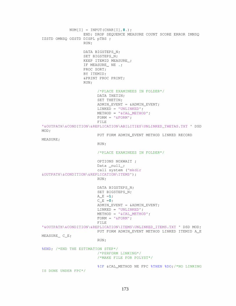
173

NUM[I] = INPUT(CHAR[I],8.); END; DROP SEQUENCE MEASURE COUNT SCORE ERROR IMNSQ IZSTD OMNSQ OZSTD DISPL pTBS ; RUN; DATA BIGSTEPS_N; SET BIGSTEPS_N; KEEP ITEMID MEASURE_; IF MEASURE_ NE .; PROC SORT; BY ITEMID; &PRINT PROC PRINT; RUN; /*PLACE EXAMINEES IN FOLDER*/ DATA THETIN; SET THETIN; ADMIN_EVENT = &ADMIN_EVENT; LINKED = "UNLINKED"; METHOD = "&CAL_METHOD"; FORM = "&FORM"; FILE "&OUTPATH\&CONDITION\&REPLICATION\ABILITIES\UNLINKED_THETAS.TXT " DSD MOD; PUT FORM ADMIN_EVENT METHOD LINKED RECORD MEASURE; RUN; /*PLACE EXAMINEES IN FOLDER*/ OPTIONS NOXWAIT ; Data _null_; call system ("mkdir &OUTPATH\&CONDITION\&REPLICATION\ITEMS"); RUN; DATA BIGSTEPS_N; SET BIGSTEPS_N; A_E =1; C_E =0; ADMIN_EVENT = &ADMIN_EVENT; LINKED = "UNLINKED"; METHOD = "&CAL_METHOD"; FORM = "&FORM"; FILE "&OUTPATH\&CONDITION\&REPLICATION\ITEMS\UNLINKED_ITEMS.TXT " DSD MOD; PUT FORM ADMIN_EVENT METHOD LINKED ITEMID A_E MEASURE_ C_E; RUN; %END; /*END THE ESTIMATION STEP*/ /*PERFORM LINKING*/ /*MAKE FILE FOR POLYST*/ %IF &CAL_METHOD NE FPC %THEN %DO;/*NO LINKING IS DONE UNDER FPC*/

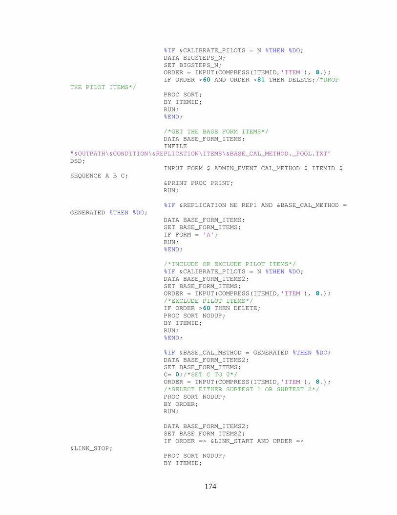
174

%IF &CALIBRATE_PILOTS = N %THEN %DO; DATA BIGSTEPS_N; SET BIGSTEPS_N; ORDER = INPUT(COMPRESS(ITEMID,'ITEM'), 8.); IF ORDER >60 AND ORDER <81 THEN DELETE;/*DROP THE PILOT ITEMS*/ PROC SORT; BY ITEMID; RUN; %END; /*GET THE BASE FORM ITEMS*/ DATA BASE_FORM_ITEMS; INFILE "&OUTPATH\&CONDITION\&REPLICATION\ITEMS\&BASE_CAL_METHOD._POOL.TXT" DSD; INPUT FORM $ ADMIN_EVENT CAL_METHOD $ ITEMID $ SEQUENCE A B C; &PRINT PROC PRINT; RUN; %IF &REPLICATION NE REP1 AND &BASE_CAL_METHOD = GENERATED %THEN %DO; DATA BASE_FORM_ITEMS; SET BASE_FORM_ITEMS; IF FORM = 'A'; RUN; %END; /*INCLUDE OR EXCLUDE PILOT ITEMS*/ %IF &CALIBRATE_PILOTS = N %THEN %DO; DATA BASE_FORM_ITEMS2; SET BASE_FORM_ITEMS; ORDER = INPUT(COMPRESS(ITEMID,'ITEM'), 8.); /*EXCLUDE PILOT ITEMS*/ IF ORDER >60 THEN DELETE; PROC SORT NODUP; BY ITEMID; RUN; %END; %IF &BASE_CAL_METHOD = GENERATED %THEN %DO; DATA BASE_FORM_ITEMS2; SET BASE_FORM_ITEMS; C= 0;/*SET C TO 0*/ ORDER = INPUT(COMPRESS(ITEMID,'ITEM'), 8.); /*SELECT EITHER SUBTEST 1 OR SUBTEST 2*/ PROC SORT NODUP; BY ORDER; RUN; DATA BASE_FORM_ITEMS2; SET BASE_FORM_ITEMS2; IF ORDER => &LINK_START AND ORDER =< &LINK_STOP; PROC SORT NODUP; BY ITEMID;

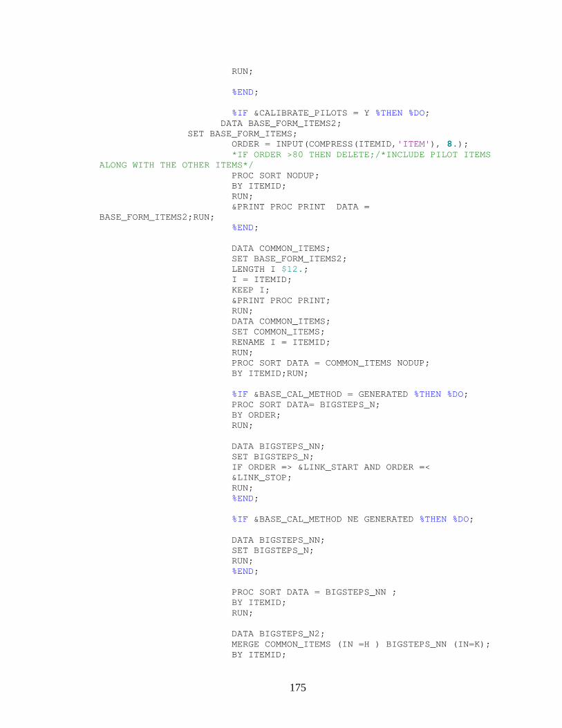
175

RUN; %END; %IF &CALIBRATE_PILOTS = Y %THEN %DO; DATA BASE_FORM_ITEMS2; SET BASE_FORM_ITEMS; ORDER = INPUT(COMPRESS(ITEMID,'ITEM'), 8.); *IF ORDER >80 THEN DELETE;/*INCLUDE PILOT ITEMS ALONG WITH THE OTHER ITEMS*/ PROC SORT NODUP; BY ITEMID; RUN; &PRINT PROC PRINT DATA = BASE_FORM_ITEMS2;RUN; %END; DATA COMMON_ITEMS; SET BASE_FORM_ITEMS2; LENGTH I $12.; I = ITEMID; KEEP I; &PRINT PROC PRINT; RUN; DATA COMMON_ITEMS; SET COMMON_ITEMS; RENAME I = ITEMID; RUN; PROC SORT DATA = COMMON_ITEMS NODUP; BY ITEMID;RUN;

%IF &BASE_CAL_METHOD = GENERATED %THEN %DO; PROC SORT DATA= BIGSTEPS_N; BY ORDER; RUN; DATA BIGSTEPS_NN; SET BIGSTEPS_N; IF ORDER => &LINK_START AND ORDER =< &LINK_STOP; RUN; %END; %IF &BASE_CAL_METHOD NE GENERATED %THEN %DO; DATA BIGSTEPS_NN; SET BIGSTEPS_N; RUN; %END;

PROC SORT DATA = BIGSTEPS_NN ; BY ITEMID; RUN; DATA BIGSTEPS_N2; MERGE COMMON_ITEMS (IN =H ) BIGSTEPS_NN (IN=K); BY ITEMID;

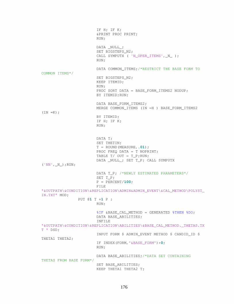
176

IF H; IF K; &PRINT PROC PRINT; RUN; DATA _NULL_; SET BIGSTEPS_N2; CALL SYMPUTX ( 'N_OPER_ITEMS',_N_ ); RUN; DATA COMMON_ITEMS;/*RESTRICT THE BASE FORM TO COMMON ITEMS*/ SET BIGSTEPS_N2; KEEP ITEMID; RUN; PROC SORT DATA = BASE_FORM_ITEMS2 NODUP; BY ITEMID;RUN; DATA BASE_FORM_ITEMS2; MERGE COMMON_ITEMS (IN =H ) BASE_FORM_ITEMS2 (IN =K); BY ITEMID; IF H; IF K; RUN; DATA T; SET THETIN; T = ROUND(MEASURE,.01); PROC FREQ DATA = T NOPRINT; TABLE T/ OUT = T_P;RUN; DATA _NULL_; SET T_P; CALL SYMPUTX ('NN',_N_);RUN; DATA T_P; /*NEWLY ESTIMATED PARAMETERS*/ SET T_P; P = PERCENT/100; FILE "&OUTPATH\&CONDITION\&REPLICATION\ADMIN&ADMIN_EVENT\&CAL_METHOD\POLYST_IN.TXT" MOD; PUT @1 T +1 P ; RUN; %IF &BASE_CAL_METHOD = GENERATED %THEN %DO; DATA BASE_ABILITIES; INFILE "&OUTPATH\&CONDITION\&REPLICATION\ABILITIES\&BASE_CAL_METHOD._THETAS.TXT " DSD; INPUT FORM $ ADMIN_EVENT METHOD $ CANDID_ID $ THETA1 THETA2; IF INDEX(FORM,"&BASE_FORM")>0; RUN; DATA BASE_ABILITIES;/*DATA SET CONTAINING THETAS FROM BASE FORM*/ SET BASE_ABILITIES; KEEP THETA1 THETA2 T;

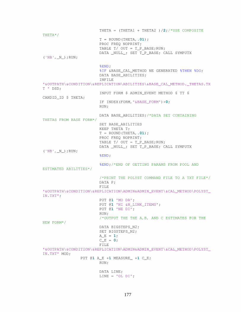
177

THETA = (THETA1 + THETA2 )/2;/*USE COMPOSITE THETA*/ T = ROUND(THETA,.01); PROC FREQ NOPRINT; TABLE T/ OUT = T_P_BASE;RUN; DATA _NULL_; SET T_P_BASE; CALL SYMPUTX ('NB',_N_);RUN; %END; %IF &BASE_CAL_METHOD NE GENERATED %THEN %DO; DATA BASE_ABILITIES; INFILE "&OUTPATH\&CONDITION\&REPLICATION\ABILITIES\&BASE_CAL_METHOD._THETAS.TXT " DSD; INPUT FORM $ ADMIN_EVENT METHOD $ TT $ CANDID_ID $ THETA; IF INDEX(FORM,"&BASE_FORM")>0; RUN; DATA BASE_ABILITIES;/*DATA SET CONTAINING THETAS FROM BASE FORM*/ SET BASE_ABILITIES KEEP THETA T; T = ROUND(THETA,.01); PROC FREQ NOPRINT; TABLE T/ OUT = T_P_BASE;RUN; DATA _NULL_; SET T_P_BASE; CALL SYMPUTX ('NB',_N_);RUN; %END; %END;/*END OF GETTING PARAMS FROM POOL AND ESTIMATED ABILITIES*/ /*PRINT THE POLYST COMMAND FILE TO A TXT FILE*/ DATA P; FILE "&OUTPATH\&CONDITION\&REPLICATION\ADMIN&ADMIN_EVENT\&CAL_METHOD\POLYST_IN.TXT"; PUT @1 "MO DR"; PUT @1 "NI &N_LINK_ITEMS"; PUT @1 "NE DI"; RUN; /*OUTPUT THE THE A,B, AND C ESTIMATES FOR THE NEW FORM*/ DATA BIGSTEPS_N2; SET BIGSTEPS_N2; A_E = 1; C_E = 0; FILE "&OUTPATH\&CONDITION\&REPLICATION\ADMIN&ADMIN_EVENT\&CAL_METHOD\POLYST_IN.TXT" MOD; PUT @1 A_E +1 MEASURE_ +1 C_E; RUN; DATA LINE; LINE = "OL DI";

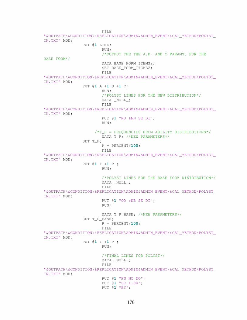
178

FILE "&OUTPATH\&CONDITION\&REPLICATION\ADMIN&ADMIN_EVENT\&CAL_METHOD\POLYST_IN.TXT" MOD; PUT @1 LINE; RUN; /*OUTPUT THE THE A,B, AND C PARAMS. FOR THE BASE FORM*/ DATA BASE_FORM_ITEMS2; SET BASE_FORM_ITEMS2; FILE "&OUTPATH\&CONDITION\&REPLICATION\ADMIN&ADMIN_EVENT\&CAL_METHOD\POLYST_IN.TXT" MOD; PUT @1 A +1 B +1 C; RUN; /*POLYST LINES FOR THE NEW DISTRIBUTION*/ DATA _NULL_; FILE "&OUTPATH\&CONDITION\&REPLICATION\ADMIN&ADMIN_EVENT\&CAL_METHOD\POLYST_IN.TXT" MOD; PUT @1 "ND &NN SE DI"; RUN; /*T_P = FREQUENCIES FROM ABILITY DISTRIBUTIONS*/ DATA T_P; /*NEW PARAMETERS*/ SET T_P; P = PERCENT/100; FILE "&OUTPATH\&CONDITION\&REPLICATION\ADMIN&ADMIN_EVENT\&CAL_METHOD\POLYST_IN.TXT" MOD; PUT @1 T +1 P ; RUN; /*POLYST LINES FOR THE BASE FORM DISTRIBUTION*/ DATA _NULL_; FILE "&OUTPATH\&CONDITION\&REPLICATION\ADMIN&ADMIN_EVENT\&CAL_METHOD\POLYST_IN.TXT" MOD; PUT @1 "OD &NB SE DI"; RUN; DATA T_P_BASE; /*NEW PARAMETERS*/ SET T_P_BASE; P = PERCENT/100; FILE "&OUTPATH\&CONDITION\&REPLICATION\ADMIN&ADMIN_EVENT\&CAL_METHOD\POLYST_IN.TXT" MOD; PUT @1 T +1 P ; RUN; /*FINAL LINES FOR POLYST*/ DATA _NULL_; FILE "&OUTPATH\&CONDITION\&REPLICATION\ADMIN&ADMIN_EVENT\&CAL_METHOD\POLYST_IN.TXT" MOD; PUT @1 "FS NO NO"; PUT @1 "SC 1.00"; PUT @1 "BY";

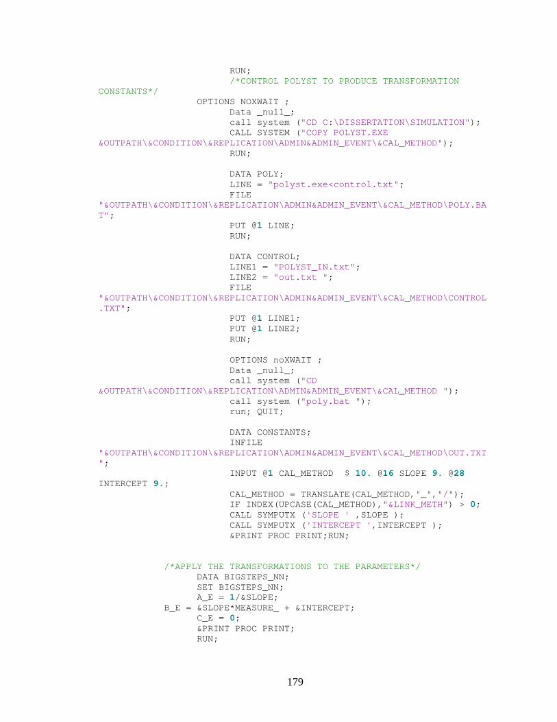
179

RUN; /*CONTROL POLYST TO PRODUCE TRANSFORMATION CONSTANTS*/ OPTIONS NOXWAIT ; Data _null_; call system ("CD C:\DISSERTATION\SIMULATION"); CALL SYSTEM ("COPY POLYST.EXE &OUTPATH\&CONDITION\&REPLICATION\ADMIN&ADMIN_EVENT\&CAL_METHOD"); RUN; DATA POLY; LINE = "polyst.exe<control.txt"; FILE "&OUTPATH\&CONDITION\&REPLICATION\ADMIN&ADMIN_EVENT\&CAL_METHOD\POLY.BAT"; PUT @1 LINE; RUN; DATA CONTROL; LINE1 = "POLYST_IN.txt"; LINE2 = "out.txt "; FILE "&OUTPATH\&CONDITION\&REPLICATION\ADMIN&ADMIN_EVENT\&CAL_METHOD\CONTROL.TXT"; PUT @1 LINE1; PUT @1 LINE2; RUN; OPTIONS noXWAIT ; Data _null_; call system ("CD &OUTPATH\&CONDITION\&REPLICATION\ADMIN&ADMIN_EVENT\&CAL_METHOD "); call system ("poly.bat "); run; QUIT; DATA CONSTANTS; INFILE "&OUTPATH\&CONDITION\&REPLICATION\ADMIN&ADMIN_EVENT\&CAL_METHOD\OUT.TXT"; INPUT @1 CAL_METHOD $ 10. @16 SLOPE 9. @28 INTERCEPT 9.; CAL_METHOD = TRANSLATE(CAL_METHOD,"_","/"); IF INDEX(UPCASE(CAL_METHOD),"&LINK_METH") > 0; CALL SYMPUTX ('SLOPE ' ,SLOPE ); CALL SYMPUTX ('INTERCEPT ',INTERCEPT ); &PRINT PROC PRINT;RUN; /*APPLY THE TRANSFORMATIONS TO THE PARAMETERS*/ DATA BIGSTEPS_NN; SET BIGSTEPS_NN; A_E = 1/&SLOPE; B_E = &SLOPE*MEASURE_ + &INTERCEPT; C_E = 0; &PRINT PROC PRINT; RUN;

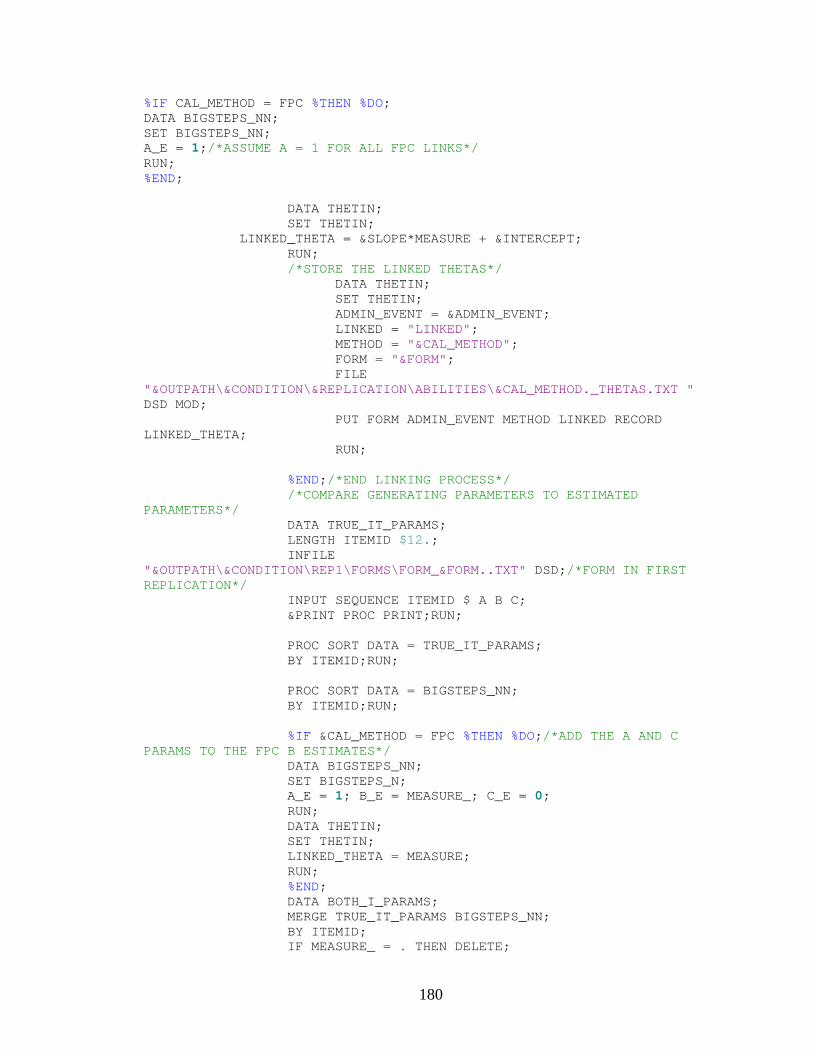
180

%IF CAL_METHOD = FPC %THEN %DO; DATA BIGSTEPS_NN; SET BIGSTEPS_NN; A_E = 1;/*ASSUME A = 1 FOR ALL FPC LINKS*/ RUN; %END; DATA THETIN; SET THETIN; LINKED_THETA = &SLOPE*MEASURE + &INTERCEPT; RUN; /*STORE THE LINKED THETAS*/ DATA THETIN; SET THETIN; ADMIN_EVENT = &ADMIN_EVENT; LINKED = "LINKED"; METHOD = "&CAL_METHOD"; FORM = "&FORM"; FILE "&OUTPATH\&CONDITION\&REPLICATION\ABILITIES\&CAL_METHOD._THETAS.TXT " DSD MOD; PUT FORM ADMIN_EVENT METHOD LINKED RECORD LINKED_THETA; RUN; %END;/*END LINKING PROCESS*/ /*COMPARE GENERATING PARAMETERS TO ESTIMATED PARAMETERS*/ DATA TRUE_IT_PARAMS; LENGTH ITEMID $12.; INFILE "&OUTPATH\&CONDITION\REP1\FORMS\FORM_&FORM..TXT" DSD;/*FORM IN FIRST REPLICATION*/ INPUT SEQUENCE ITEMID $ A B C; &PRINT PROC PRINT;RUN; PROC SORT DATA = TRUE_IT_PARAMS; BY ITEMID;RUN; PROC SORT DATA = BIGSTEPS_NN; BY ITEMID;RUN; %IF &CAL_METHOD = FPC %THEN %DO;/*ADD THE A AND C PARAMS TO THE FPC B ESTIMATES*/ DATA BIGSTEPS_NN; SET BIGSTEPS_N; A_E = 1; B_E = MEASURE_; C_E = 0; RUN; DATA THETIN; SET THETIN; LINKED_THETA = MEASURE; RUN; %END; DATA BOTH_I_PARAMS; MERGE TRUE_IT_PARAMS BIGSTEPS_NN; BY ITEMID; IF MEASURE_ = . THEN DELETE;

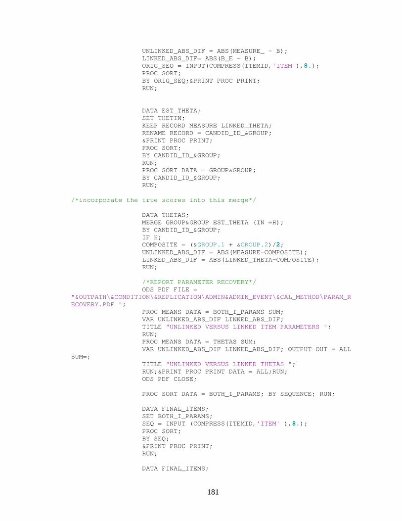
181

UNLINKED_ABS_DIF = ABS(MEASURE_ - B); LINKED_ABS_DIF= ABS(B_E - B); ORIG_SEQ = INPUT(COMPRESS(ITEMID,'ITEM'),8.); PROC SORT; BY ORIG_SEQ;&PRINT PROC PRINT; RUN; DATA EST_THETA; SET THETIN; KEEP RECORD MEASURE LINKED_THETA; RENAME RECORD = CANDID_ID_&GROUP; &PRINT PROC PRINT; PROC SORT; BY CANDID_ID_&GROUP; RUN; PROC SORT DATA = GROUP&GROUP; BY CANDID_ID_&GROUP; RUN; /*incorporate the true scores into this merge*/ DATA THETAS; MERGE GROUP&GROUP EST_THETA (IN =H); BY CANDID_ID_&GROUP; IF H; COMPOSITE = (&GROUP.1 + &GROUP.2)/2; UNLINKED_ABS_DIF = ABS(MEASURE-COMPOSITE); LINKED_ABS_DIF = ABS(LINKED_THETA-COMPOSITE); RUN; /*REPORT PARAMETER RECOVERY*/ ODS PDF FILE = "&OUTPATH\&CONDITION\&REPLICATION\ADMIN&ADMIN_EVENT\&CAL_METHOD\PARAM_RECOVERY.PDF "; PROC MEANS DATA = BOTH_I_PARAMS SUM; VAR UNLINKED_ABS_DIF LINKED_ABS_DIF; TITLE "UNLINKED VERSUS LINKED ITEM PARAMETERS "; RUN; PROC MEANS DATA = THETAS SUM; VAR UNLINKED_ABS_DIF LINKED_ABS_DIF; OUTPUT OUT = ALL SUM=; TITLE "UNLINKED VERSUS LINKED THETAS "; RUN;&PRINT PROC PRINT DATA = ALL;RUN; ODS PDF CLOSE; PROC SORT DATA = BOTH_I_PARAMS; BY SEQUENCE; RUN; DATA FINAL_ITEMS; SET BOTH_I_PARAMS; SEQ = INPUT (COMPRESS(ITEMID,'ITEM' ),8.); PROC SORT; BY SEQ; &PRINT PROC PRINT; RUN; DATA FINAL_ITEMS;

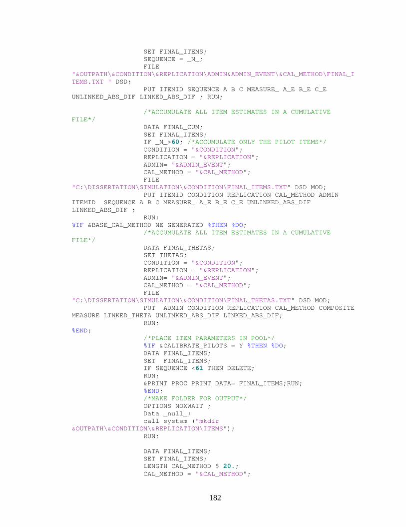
182

SET FINAL_ITEMS; SEQUENCE = _N_; FILE "&OUTPATH\&CONDITION\&REPLICATION\ADMIN&ADMIN_EVENT\&CAL_METHOD\FINAL_ITEMS.TXT " DSD; PUT ITEMID SEQUENCE A B C MEASURE_ A_E B_E C_E UNLINKED_ABS_DIF LINKED_ABS_DIF ; RUN; /*ACCUMULATE ALL ITEM ESTIMATES IN A CUMULATIVE FILE*/ DATA FINAL_CUM; SET FINAL_ITEMS; IF _N_>60; /*ACCUMULATE ONLY THE PILOT ITEMS*/ CONDITION = "&CONDITION"; REPLICATION = "&REPLICATION"; ADMIN= "&ADMIN_EVENT"; CAL_METHOD = "&CAL_METHOD"; FILE "C:\DISSERTATION\SIMULATION\&CONDITION\FINAL_ITEMS.TXT" DSD MOD; PUT ITEMID CONDITION REPLICATION CAL_METHOD ADMIN ITEMID SEQUENCE A B C MEASURE_ A_E B_E C_E UNLINKED_ABS_DIF LINKED_ABS_DIF ; RUN; %IF &BASE_CAL_METHOD NE GENERATED %THEN %DO; /*ACCUMULATE ALL ITEM ESTIMATES IN A CUMULATIVE FILE*/ DATA FINAL_THETAS; SET THETAS; CONDITION = "&CONDITION"; REPLICATION = "&REPLICATION"; ADMIN= "&ADMIN_EVENT"; CAL_METHOD = "&CAL_METHOD"; FILE "C:\DISSERTATION\SIMULATION\&CONDITION\FINAL_THETAS.TXT" DSD MOD; PUT ADMIN CONDITION REPLICATION CAL_METHOD COMPOSITE MEASURE LINKED_THETA UNLINKED_ABS_DIF LINKED_ABS_DIF; RUN; %END; /*PLACE ITEM PARAMETERS IN POOL*/ %IF &CALIBRATE_PILOTS = Y %THEN %DO; DATA FINAL_ITEMS; SET FINAL_ITEMS; IF SEQUENCE <61 THEN DELETE; RUN; &PRINT PROC PRINT DATA= FINAL_ITEMS;RUN; %END; /*MAKE FOLDER FOR OUTPUT*/ OPTIONS NOXWAIT ; Data _null_; call system ("mkdir &OUTPATH\&CONDITION\&REPLICATION\ITEMS"); RUN; DATA FINAL_ITEMS; SET FINAL_ITEMS; LENGTH CAL_METHOD $ 20.; CAL_METHOD = "&CAL_METHOD";

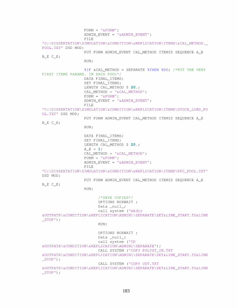
183

FORM = "&FORM"; ADMIN_EVENT = "&ADMIN_EVENT"; FILE "C:\DISSERTATION\SIMULATION\&CONDITION\&REPLICATION\ITEMS\&CAL_METHOD._POOL.TXT" DSD MOD; PUT FORM ADMIN_EVENT CAL_METHOD ITEMID SEQUENCE A_E B_E C_E; RUN; %IF &CAL_METHOD = SEPARATE %THEN %DO; /*PUT THE VERY FIRST ITEMS PARAMS. IN EACH POOL*/ DATA FINAL_ITEMS; SET FINAL_ITEMS; LENGTH CAL_METHOD $ 20.; CAL_METHOD = "&CAL_METHOD"; FORM = "&FORM"; ADMIN_EVENT = "&ADMIN_EVENT"; FILE "C:\DISSERTATION\SIMULATION\&CONDITION\&REPLICATION\ITEMS\STOCK_LORD_POOL.TXT" DSD MOD; PUT FORM ADMIN_EVENT CAL_METHOD ITEMID SEQUENCE A_E B_E C_E; RUN; DATA FINAL_ITEMS; SET FINAL_ITEMS; LENGTH CAL_METHOD $ 20.; A_E = 1; CAL_METHOD = "&CAL_METHOD"; FORM = "&FORM"; ADMIN_EVENT = "&ADMIN_EVENT"; FILE "C:\DISSERTATION\SIMULATION\&CONDITION\&REPLICATION\ITEMS\FPC_POOL.TXT" DSD MOD; PUT FORM ADMIN_EVENT CAL_METHOD ITEMID SEQUENCE A_E B_E C_E; RUN; /*SAVE COPIES*/ OPTIONS NOXWAIT ; Data _null_; call system ("mkdir &OUTPATH\&CONDITION\&REPLICATION\ADMIN1\SEPARATE\SET&LINK_START.TO&LINK_STOP"); RUN; OPTIONS NOXWAIT ; Data _null_; call system ("CD &OUTPATH\&CONDITION\&REPLICATION\ADMIN1\SEPARATE"); CALL SYSTEM ("COPY POLYST_IN.TXT &OUTPATH\&CONDITION\&REPLICATION\ADMIN1\SEPARATE\SET&LINK_START.TO&LINK_STOP"); CALL SYSTEM ("COPY OUT.TXT &OUTPATH\&CONDITION\&REPLICATION\ADMIN1\SEPARATE\SET&LINK_START.TO&LINK_STOP");

184

CALL SYSTEM ("COPY FINAL_ITEMS.TXT &OUTPATH\&CONDITION\&REPLICATION\ADMIN1\SEPARATE\SET&LINK_START.TO&LINK_STOP"); RUN; %END; %MEND; %GLOBAL T F TS;

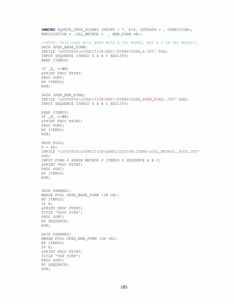
185

%MACRO EQUATE_TRUE_SCORES (PRINT = *, D=1, OUTPATH = , CONDITION=, REPLICATION = ,CAL_METHOD = , NEW_FORM =B); /*NOTE: THIS CODE WILL WORK WITH A 1PL MODEL, NOT A 2 OR 3PL MODEL*/ DATA OPER_BASE_FORM; INFILE "&OUTPATH\&CONDITION\REP1\FORMS\FORM_A.TXT" DSD; INPUT SEQUENCE ITEMID $ A B C ABILITY; KEEP ITEMID; IF _N_ =<60; &PRINT PROC PRINT; PROC SORT; BY ITEMID; RUN; DATA OPER_NEW_FORM; INFILE "&OUTPATH\&CONDITION\REP1\FORMS\FORM_&NEW_FORM..TXT" DSD; INPUT SEQUENCE ITEMID $ A B C ABILITY; KEEP ITEMID; IF _N_ =<60; &PRINT PROC PRINT; PROC SORT; BY ITEMID; RUN; DATA POOL; D = &D; INFILE "&OUTPATH\&CONDITION\&REPLICATION\ITEMS\&CAL_METHOD._POOL.TXT" DSD; INPUT FORM $ ADMIN METHOD $ ITEMID $ SEQUENCE A B C; &PRINT PROC PRINT; PROC SORT; BY ITEMID; RUN; DATA PARAMS1; MERGE POOL OPER_BASE_FORM (IN =H); BY ITEMID; IF H; &PRINT PROC PRINT; TITLE "BASE FORM"; PROC SORT; BY SEQUENCE; RUN; DATA PARAMS2; MERGE POOL OPER_NEW_FORM (IN =H); BY ITEMID; IF H; &PRINT PROC PRINT; TITLE "NEW FORM"; PROC SORT; BY SEQUENCE; RUN;

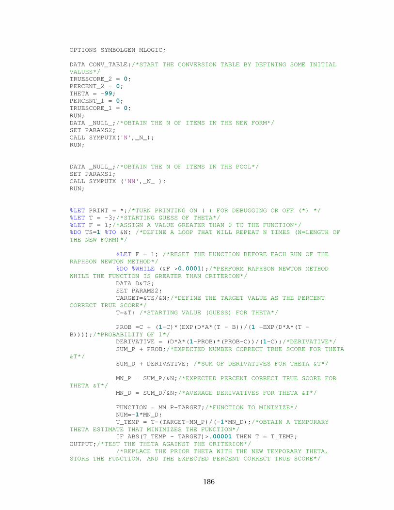
186

OPTIONS SYMBOLGEN MLOGIC; DATA CONV_TABLE;/*START THE CONVERSION TABLE BY DEFINING SOME INITIAL VALUES*/ TRUESCORE_2 = 0; PERCENT_2 = 0; THETA = -99; PERCENT_1 = 0; TRUESCORE_1 = 0; RUN; DATA _NULL_;/*OBTAIN THE N OF ITEMS IN THE NEW FORM*/ SET PARAMS2; CALL SYMPUTX('N',_N_); RUN; DATA _NULL_;/*OBTAIN THE N OF ITEMS IN THE POOL*/ SET PARAMS1; CALL SYMPUTX ('NN',_N_ ); RUN; %LET PRINT = *;/*TURN PRINTING ON ( ) FOR DEBUGGING OR OFF (*) */ %LET T = -3;/*STARTING GUESS OF THETA*/ %LET F = 1;/*ASSIGN A VALUE GREATER THAN 0 TO THE FUNCTION*/ %DO TS=1 %TO &N; /*DEFINE A LOOP THAT WILL REPEAT N TIMES (N=LENGTH OF THE NEW FORM)*/ %LET F = 1; /*RESET THE FUNCTION BEFORE EACH RUN OF THE RAPHSON NEWTON METHOD*/ %DO %WHILE (&F >0.0001);/*PERFORM RAPHSON NEWTON METHOD WHILE THE FUNCTION IS GREATER THAN CRITERION*/ DATA D&TS; SET PARAMS2; TARGET=&TS/&N;/*DEFINE THE TARGET VALUE AS THE PERCENT CORRECT TRUE SCORE*/ T=&T; /*STARTING VALUE (GUESS) FOR THETA*/ PROB =C + (1-C)*(EXP(D*A*(T - B))/(1 +EXP(D*A*(T - B))));/*PROBABILITY OF 1*/ DERIVATIVE = (D*A*(1-PROB)*(PROB-C))/(1-C);/*DERIVATIVE*/ SUM_P + PROB;/*EXPECTED NUMBER CORRECT TRUE SCORE FOR THETA &T*/ SUM_D + DERIVATIVE; /*SUM OF DERIVATIVES FOR THETA &T*/ MN_P = SUM_P/&N;/*EXPECTED PERCENT CORRECT TRUE SCORE FOR THETA &T*/ MN_D = SUM_D/&N;/*AVERAGE DERIVATIVES FOR THETA &T*/ FUNCTION = MN_P-TARGET;/*FUNCTION TO MINIMIZE*/ NUM=-1*MN_D; T_TEMP = T-(TARGET-MN_P)/(-1*MN_D);/*OBTAIN A TEMPORARY THETA ESTIMATE THAT MINIMIZES THE FUNCTION*/ IF ABS(T_TEMP - TARGET)>.00001 THEN T = T_TEMP; OUTPUT;/*TEST THE THETA AGAINST THE CRITERION*/ /*REPLACE THE PRIOR THETA WITH THE NEW TEMPORARY THETA, STORE THE FUNCTION, AND THE EXPECTED PERCENT CORRECT TRUE SCORE*/

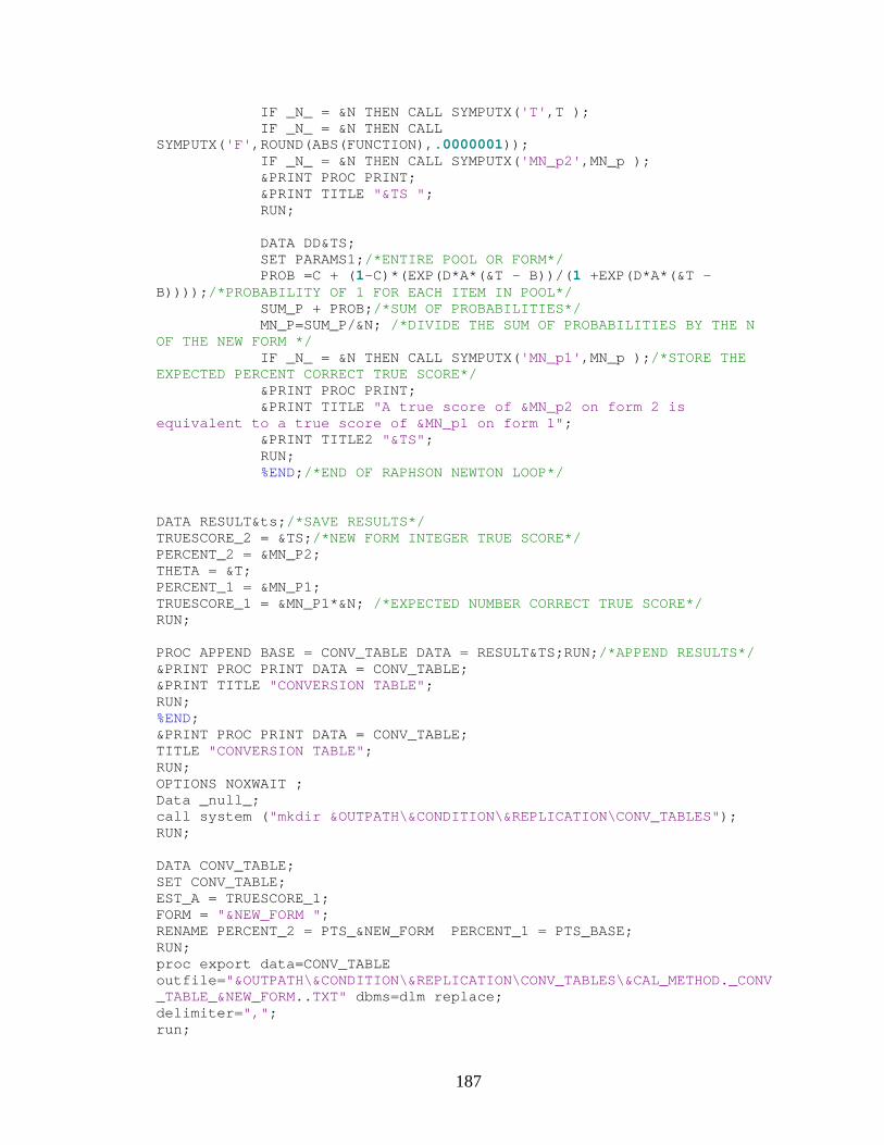
187

IF _N_ = &N THEN CALL SYMPUTX('T',T ); IF _N_ = &N THEN CALL SYMPUTX('F',ROUND(ABS(FUNCTION),.0000001)); IF _N_ = &N THEN CALL SYMPUTX('MN_p2',MN_p ); &PRINT PROC PRINT; &PRINT TITLE "&TS "; RUN; DATA DD&TS; SET PARAMS1;/*ENTIRE POOL OR FORM*/ PROB =C + (1-C)*(EXP(D*A*(&T - B))/(1 +EXP(D*A*(&T - B))));/*PROBABILITY OF 1 FOR EACH ITEM IN POOL*/ SUM_P + PROB;/*SUM OF PROBABILITIES*/ MN_P=SUM_P/&N; /*DIVIDE THE SUM OF PROBABILITIES BY THE N OF THE NEW FORM */ IF _N_ = &N THEN CALL SYMPUTX('MN_p1',MN_p );/*STORE THE EXPECTED PERCENT CORRECT TRUE SCORE*/ &PRINT PROC PRINT; &PRINT TITLE "A true score of &MN_p2 on form 2 is equivalent to a true score of &MN_p1 on form 1"; &PRINT TITLE2 "&TS"; RUN; %END;/*END OF RAPHSON NEWTON LOOP*/ DATA RESULT&ts;/*SAVE RESULTS*/ TRUESCORE_2 = &TS;/*NEW FORM INTEGER TRUE SCORE*/ PERCENT_2 = &MN_P2; THETA = &T; PERCENT_1 = &MN_P1; TRUESCORE_1 = &MN_P1*&N; /*EXPECTED NUMBER CORRECT TRUE SCORE*/ RUN; PROC APPEND BASE = CONV_TABLE DATA = RESULT&TS;RUN;/*APPEND RESULTS*/ &PRINT PROC PRINT DATA = CONV_TABLE; &PRINT TITLE "CONVERSION TABLE"; RUN; %END; &PRINT PROC PRINT DATA = CONV_TABLE; TITLE "CONVERSION TABLE"; RUN; OPTIONS NOXWAIT ; Data _null_; call system ("mkdir &OUTPATH\&CONDITION\&REPLICATION\CONV_TABLES"); RUN; DATA CONV_TABLE; SET CONV_TABLE; EST_A = TRUESCORE_1; FORM = "&NEW_FORM "; RENAME PERCENT_2 = PTS_&NEW_FORM PERCENT_1 = PTS_BASE; RUN; proc export data=CONV_TABLE outfile="&OUTPATH\&CONDITION\&REPLICATION\CONV_TABLES\&CAL_METHOD._CONV_TABLE_&NEW_FORM..TXT" dbms=dlm replace; delimiter=","; run;

188

DATA CUM_CONV_TABLE; SET CONV_TABLE; FORM = "&NEW_FORM"; REPLICATION = "&REPLICATION"; FILE "&OUTPATH\&CONDITION\&CAL_METHOD._CONV_TABLE.TXT " MOD; PUT FORM REPLICATION TRUESCORE_2 THETA EST_A; RUN; /*COMPARE TO CRITERION CONV. TABLE*/ DATA CRITERION_CONV_TABLE; INFILE "&OUTPATH\&CONDITION\EQUIPERCENTILE_CONV_TABLE.TXT " MOD; INPUT FORM $ TRUESCORE_2 A ; RUN; DATA CONV_TABLE; MERGE CRITERION_CONV_TABLE CONV_TABLE (IN =H); BY FORM TRUESCORE_2; IF H; RUN; DATA CUM_CONV_TABLE; SET CONV_TABLE; METHOD = "&CAL_METHOD"; REPLICATION = "&REPLICATION"; FILE "&OUTPATH\&CONDITION\DIFFERENCE.TXT " MOD DSD; PUT METHOD FORM REPLICATION TRUESCORE_2 A EST_A; RUN; &PRINT PROC PRINT DATA = CUM_CONV_TABLE;RUN; /*EMPTY THE CONV. TABLE */ DATA CONV_TABLE; RUN; %MEND;

189

/******************************************************************/ /* PURPOSE OF MACRO IS TO PERFORM LINEAR EQUATING */ /* PERFORMS: */ /* 1. TUCKER LINEAR EQUATING */ /* 2. LEVINE LINEAR EQUATING */ /* 3. LEVINE TRUE SCORE EQUATING */ /* */ /* PROGRAM ALSO IMPLEMENTS MANTEL HAENZEL DELTA DIF AND REMOVES*/ /* ITEMS FLAGGED WITH SEVERE DIF */ /* */ /* NITEMS = NUMBER OF ITEMS ON TEST */ /* CUT = NUMBER CORRECT RAW CUT SCORE */ /* REMOVE_C = Y =YES, REMOVE ITEMS FLAGGED WITH DIF AT LEVEL 'C' */ /* PASSFAIL = Y =YES, CALCULATE PASS/FAIL */ /* ROUND_BUF = AMOUNT TO ADJUST SCALE, MAY BE USED TO ADJUST SCALE */ /* ODSOUT = */ /* BASE = NAME OF BASE FORM */ /* NEWFORM = NAME OF NEW FORM */ /* _A_ = SLOPE OF LINEAR SCALE CONVERSION */ /* _B_ = INTERCEPT FOR LINEAR SCALE CONVERSION */ /* CIPE = Y = , SEND DATA OUT FOR CIPE */ /* PRINT = IF * THE DO NOT PRINT ALL DATA SETS */ /* ROUND_SCALE = IF Y THEN ROUND THE SCORE SCALE TO NEAREST WHOLE N */ /* */ /******************************************************************/ %MACRO LINEAR_EQUATE (folder_path= C:\EHT\, CONDITION = COND1,REPLICATION = REP1,ADMIN_EVENT = 1, NITEMS =60, CUT = 55, REMOVE_C = , PASSFAIL =, ROUND_BUF = ,ODSOUT =, OUTPATH =, BASE =, NEWFORM = , _A_ = 1, _B_ = 1, CIPE = N, PRINT = *,ROUND_SCALE=, NEW_ADMIN =2, BASE_ADMIN = 1, MONTH = ); libname l "&folder_path"; /*GET THE BASE FORM*/ DATA BASE; infile "c:\eht\xeaa.txt " truncover dsd delimiter='09'x; INPUT AN606 AN69 AN250 AN476 AN94 AN216 AN701 AN687 AN37 AN309 AN412 AN361 AN6 AN697 AN471 AN237 AN225 AN387 AN550 AN296 AN209 AN544 AN441 AN299 AN671 AN614 AN626 AN206 AN398 AN386 AN593 AN462 AN561 AN820 AN194 AN494 AN819 AN396 AN113 AN263 AN290 AN584 AN49 AN201 AN124 AN463 AN813 AN224 AN435 AN700 AN182 AN668 AN633 AN326 AN664 AN578 AN198 AN456 AN465 AN622 AN538 AN654 AN159 AN43 AN353 AN684 AN647 AN586 AN514 AN355 AN481 AN52 AN308 AN336 AN103 AN251 AN590 AN63 AN812 AN411; rscore = sum (of _NUMERIC_); proc print;run; data BASE; set base; RAW_SCORE2 = RSCORE; run;

190

PROC FREQ DATA = BASE NOPRINT; TABLE RAW_SCORE2/ OUT= BASEFREQ; RUN; DATA BASEFREQ; SET BASEFREQ; RENAME COUNT = BASE_COUNT PERCENT = BASE_PERCENT; RUN; /*GET NEW ITEMS*/ DATA NEWFORM; SET L.MATRIX&NEWFORM; RUN; /*SAVE COPIES*/ OPTIONS NOXWAIT ; Data _null_; call system ("mkdir &OUTPATH\&NEWFORM"); RUN; DATA DELETED; SET NEWFORM; IF RAW_SCORE2 = 0; PROC PRINT; RUN; proc export data=DELETED outfile="&OUTPATH\&NEWFORM\DELETED.TXT" dbms=dlm replace; delimiter=","; run; /*REMOVE ANY SCORES OF 0*/ DATA NEWFORM; SET NEWFORM; IF RAW_SCORE2 = 0 THEN DELETE; RUN; PROC FREQ DATA = NEWFORM NOPRINT; TABLE RAW_SCORE2/ OUT= NEWFREQ; RUN; data freqs; retain raw_score2 base_count count base_percent percent; merge basefreq newfreq; by raw_score2; rename count = new_count percent = new_percent; proc print;run; proc export data=freqs outfile="&OUTPATH\&NEWFORM\FREQUENCIES.TXT" dbms=dlm replace; delimiter=","; run; PROC CONTENTS DATA = NEWFORM OUT = ITEMIDS;RUN;

191

DATA T_N; SET ITEMIDS; CALL SYMPUTX ('N_OBS', NOBS ); IF SUBSTRN(NAME,1,2)= "AN"; RENAME NAME =ITEMID1 ; NEWFORM =1; KEEP NAME NEWFORM; PROC SORT; BY ITEMID1; PROC PRINT;RUN; PROC SORT DATA = T_B; BY ITEMID1;RUN; PROC SQL NOPRINT; SELECT DISTINCT ITEMID1 INTO: NEW_ITEMS SEPARATED BY " " FROM T_N ORDER BY ITEMID1; QUIT; %PUT &NEW_ITEMS; /*NOW BASE ITEMS*/ PROC CONTENTS DATA = BASE OUT = ITEMIDSB;RUN; DATA T_B; SET ITEMIDSB; IF SUBSTRN(NAME,1,2)= "AN"; RENAME NAME =ITEMID1 ; NEWFORM =1; KEEP NAME NEWFORM; PROC SORT; BY ITEMID1; PROC PRINT;RUN; PROC SORT DATA = T_B; BY ITEMID1;RUN; PROC SQL NOPRINT; SELECT DISTINCT ITEMID1 INTO: BASE_ITEMS SEPARATED BY " " FROM T_B ORDER BY ITEMID1; QUIT; %PUT &BASE_ITEMS; /*COMBINE THEM TO ISOLATE THE COMMON ITEMS*/ DATA ITEMLIST; MERGE T_N (IN=U) T_B (IN=Y); BY ITEMID1; IF U; IF Y; &PRINT PROC PRINT; RUN; PROC SQL NOPRINT;

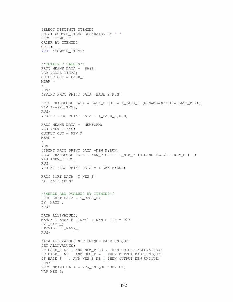
192

SELECT DISTINCT ITEMID1 INTO: COMMON_ITEMS SEPARATED BY " " FROM ITEMLIST ORDER BY ITEMID1; QUIT; %PUT &COMMON_ITEMS; /*OBTAIN P VALUES*/ PROC MEANS DATA = BASE; VAR &BASE_ITEMS; OUTPUT OUT = BASE_P MEAN = ; RUN; &PRINT PROC PRINT DATA =BASE_P;RUN; PROC TRANSPOSE DATA = BASE_P OUT = T_BASE_P (RENAME=(COL1 = BASE_P )); VAR &BASE_ITEMS; RUN; &PRINT PROC PRINT DATA = T_BASE_P;RUN; PROC MEANS DATA = NEWFORM; VAR &NEW_ITEMS; OUTPUT OUT = NEW_P MEAN = ; RUN; &PRINT PROC PRINT DATA =NEW_P;RUN; PROC TRANSPOSE DATA = NEW_P OUT = T_NEW_P (RENAME=(COL1 = NEW_P ) ); VAR &NEW_ITEMS; RUN; &PRINT PROC PRINT DATA = T_NEW_P;RUN; PROC SORT DATA =T_NEW_P; BY _NAME_;RUN; /*MERGE ALL PVALUES BY ITEMIDS*/ PROC SORT DATA = T_BASE_P; BY _NAME_; RUN; DATA ALLPVALUES; MERGE T_BASE_P (IN=Y) T_NEW_P (IN = U); BY _NAME_; ITEMID1 = _NAME_; RUN; DATA ALLPVALUES NEW_UNIQUE BASE_UNIQUE; SET ALLPVALUES; IF BASE_P NE . AND NEW_P NE . THEN OUTPUT ALLPVALUES; IF BASE_P NE . AND NEW_P = . THEN OUTPUT BASE_UNIQUE; IF BASE_P = . AND NEW_P NE . THEN OUTPUT NEW_UNIQUE; RUN; PROC MEANS DATA = NEW_UNIQUE NOPRINT; VAR NEW_P;

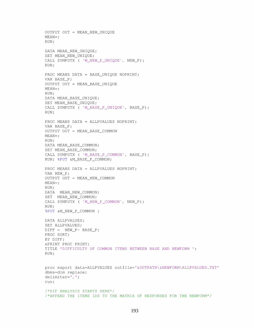
193

OUTPUT OUT = MEAN_NEW_UNIQUE MEAN=; RUN; DATA MEAN_NEW_UNIQUE; SET MEAN_NEW_UNIQUE; CALL SYMPUTX ( 'M_NEW_P_UNIQUE', NEW_P); RUN; PROC MEANS DATA = BASE_UNIQUE NOPRINT; VAR BASE_P; OUTPUT OUT = MEAN_BASE_UNIQUE MEAN=; RUN; DATA MEAN_BASE_UNIQUE; SET MEAN_BASE_UNIQUE; CALL SYMPUTX ( 'M_BASE_P_UNIQUE', BASE_P); RUN; PROC MEANS DATA = ALLPVALUES NOPRINT; VAR BASE_P; OUTPUT OUT = MEAN_BASE_COMMON MEAN=; RUN; DATA MEAN_BASE_COMMON; SET MEAN_BASE_COMMON; CALL SYMPUTX ( 'M_BASE_P_COMMON', BASE_P); RUN; %PUT &M_BASE_P_COMMON; PROC MEANS DATA = ALLPVALUES NOPRINT; VAR NEW_P; OUTPUT OUT = MEAN_NEW_COMMON MEAN=; RUN; DATA MEAN_NEW_COMMON; SET MEAN_NEW_COMMON; CALL SYMPUTX ( 'M_NEW_P_COMMON', NEW_P); RUN; %PUT &M_NEW_P_COMMON ; DATA ALLPVALUES; SET ALLPVALUES; DIFF = NEW_P- BASE_P; PROC SORT; BY DIFF; &PRINT PROC PRINT; TITLE "DIFFICULTY OF COMMON ITEMS BETWEEN BASE AND NEWFORM "; RUN; proc export data=ALLPVALUES outfile="&OUTPATH\&NEWFORM\ALLPVALUES.TXT" dbms=dlm replace; delimiter=","; run; /*DIF ANALYSIS STARTS HERE*/ /*APPEND THE ITEMS IDS TO THE MATRIX OF RESPONSES FOR THE NEWFORM*/

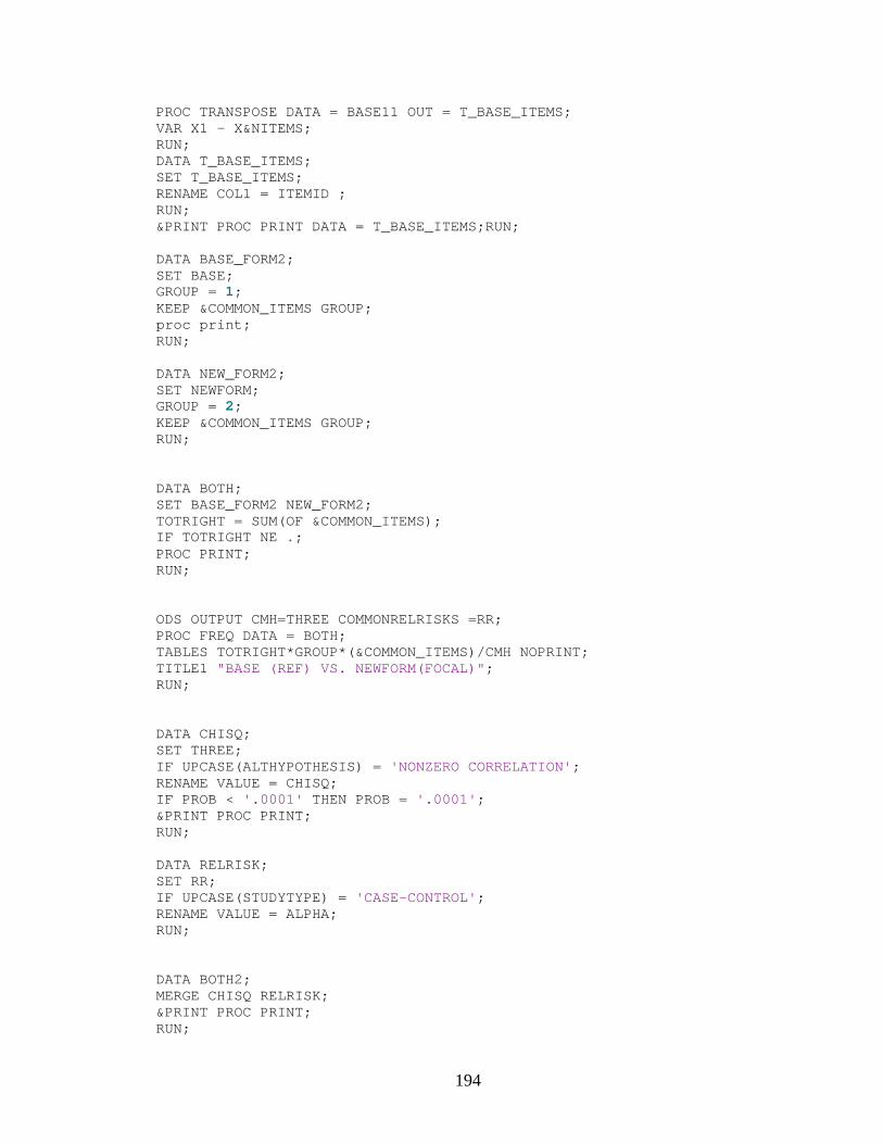
194

PROC TRANSPOSE DATA = BASE11 OUT = T_BASE_ITEMS; VAR X1 - X&NITEMS; RUN; DATA T_BASE_ITEMS; SET T_BASE_ITEMS; RENAME COL1 = ITEMID ; RUN; &PRINT PROC PRINT DATA = T_BASE_ITEMS;RUN; DATA BASE_FORM2; SET BASE; GROUP = 1; KEEP &COMMON_ITEMS GROUP; proc print; RUN; DATA NEW_FORM2; SET NEWFORM; GROUP = 2; KEEP &COMMON_ITEMS GROUP; RUN; DATA BOTH; SET BASE_FORM2 NEW_FORM2; TOTRIGHT = SUM(OF &COMMON_ITEMS); IF TOTRIGHT NE .; PROC PRINT; RUN; ODS OUTPUT CMH=THREE COMMONRELRISKS =RR; PROC FREQ DATA = BOTH; TABLES TOTRIGHT*GROUP*(&COMMON_ITEMS)/CMH NOPRINT; TITLE1 "BASE (REF) VS. NEWFORM(FOCAL)"; RUN; DATA CHISQ; SET THREE; IF UPCASE(ALTHYPOTHESIS) = 'NONZERO CORRELATION'; RENAME VALUE = CHISQ; IF PROB < '.0001' THEN PROB = '.0001'; &PRINT PROC PRINT; RUN; DATA RELRISK; SET RR; IF UPCASE(STUDYTYPE) = 'CASE-CONTROL'; RENAME VALUE = ALPHA; RUN; DATA BOTH2; MERGE CHISQ RELRISK; &PRINT PROC PRINT; RUN;

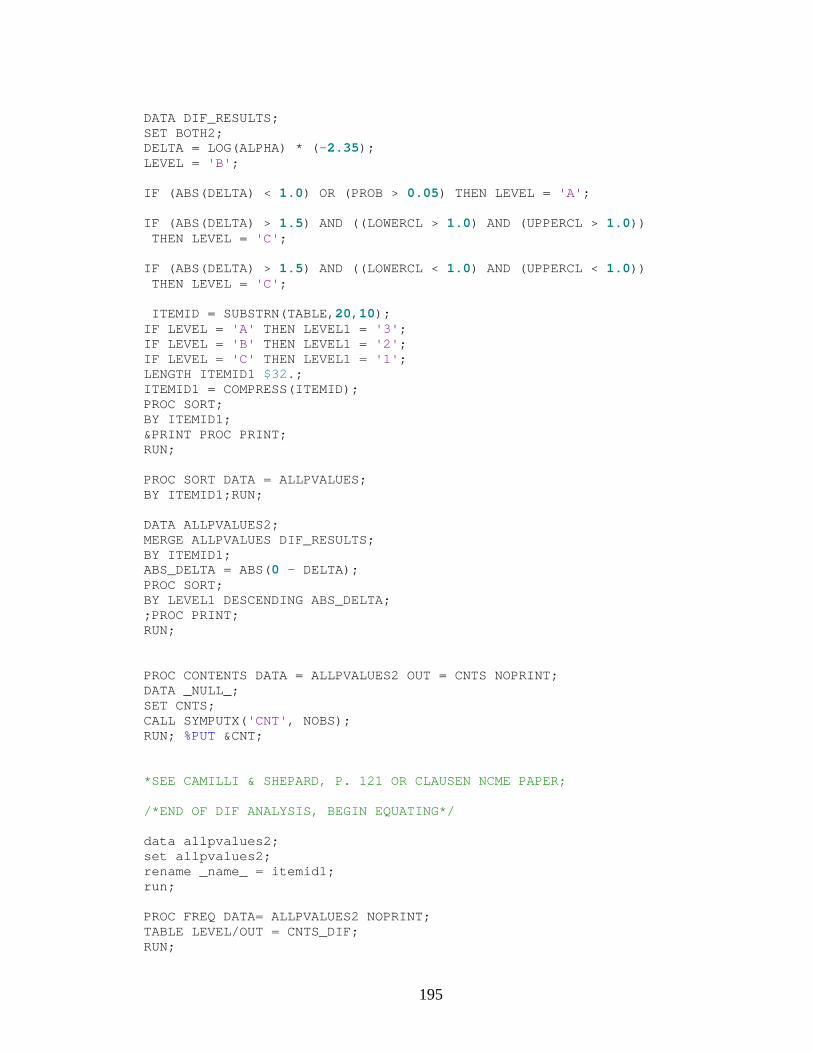
195

DATA DIF_RESULTS; SET BOTH2; DELTA = LOG(ALPHA) * (-2.35); LEVEL = 'B'; IF (ABS(DELTA) < 1.0) OR (PROB > 0.05) THEN LEVEL = 'A'; IF (ABS(DELTA) > 1.5) AND ((LOWERCL > 1.0) AND (UPPERCL > 1.0)) THEN LEVEL = 'C'; IF (ABS(DELTA) > 1.5) AND ((LOWERCL < 1.0) AND (UPPERCL < 1.0)) THEN LEVEL = 'C'; ITEMID = SUBSTRN(TABLE,20,10); IF LEVEL = 'A' THEN LEVEL1 = '3'; IF LEVEL = 'B' THEN LEVEL1 = '2'; IF LEVEL = 'C' THEN LEVEL1 = '1'; LENGTH ITEMID1 $32.; ITEMID1 = COMPRESS(ITEMID); PROC SORT; BY ITEMID1; &PRINT PROC PRINT; RUN; PROC SORT DATA = ALLPVALUES; BY ITEMID1;RUN; DATA ALLPVALUES2; MERGE ALLPVALUES DIF_RESULTS; BY ITEMID1; ABS_DELTA = ABS(0 - DELTA); PROC SORT; BY LEVEL1 DESCENDING ABS_DELTA; ;PROC PRINT; RUN; PROC CONTENTS DATA = ALLPVALUES2 OUT = CNTS NOPRINT; DATA _NULL_; SET CNTS; CALL SYMPUTX('CNT', NOBS); RUN; %PUT &CNT; *SEE CAMILLI & SHEPARD, P. 121 OR CLAUSEN NCME PAPER; /*END OF DIF ANALYSIS, BEGIN EQUATING*/ data allpvalues2; set allpvalues2; rename _name_ = itemid1; run; PROC FREQ DATA= ALLPVALUES2 NOPRINT; TABLE LEVEL/OUT = CNTS_DIF; RUN;

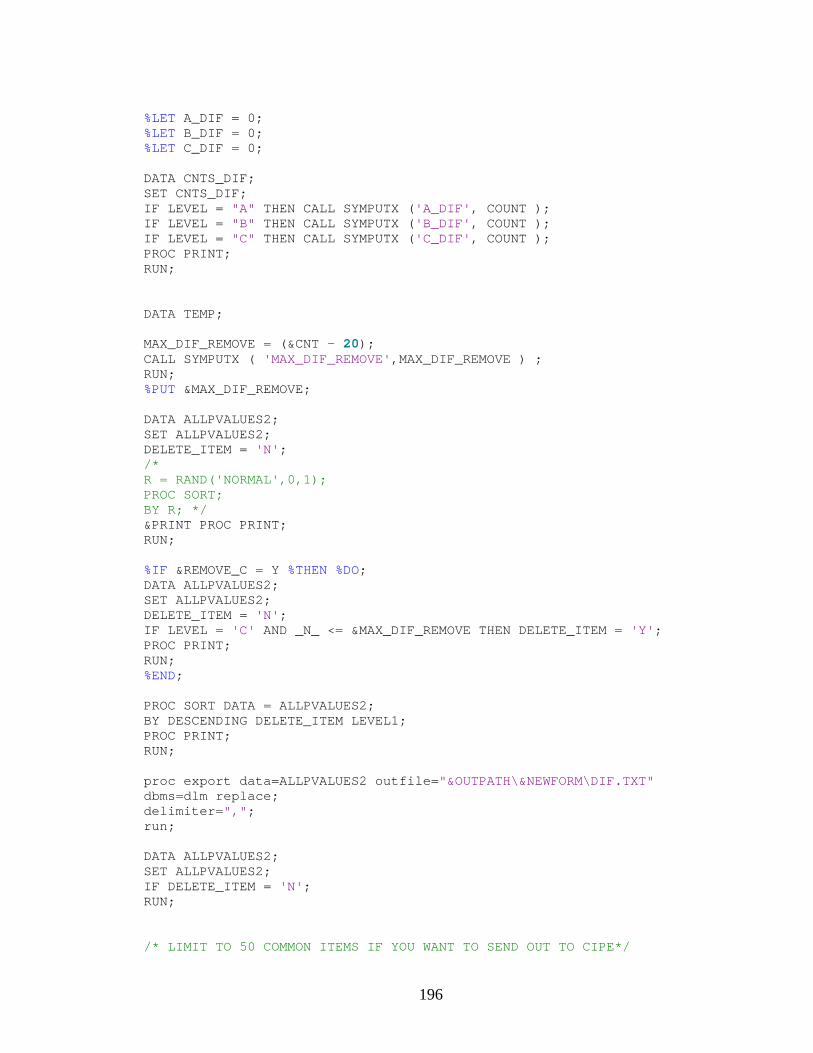
196

%LET A_DIF = 0; %LET B_DIF = 0; %LET C_DIF = 0; DATA CNTS_DIF; SET CNTS_DIF; IF LEVEL = "A" THEN CALL SYMPUTX ('A_DIF', COUNT ); IF LEVEL = "B" THEN CALL SYMPUTX ('B_DIF', COUNT ); IF LEVEL = "C" THEN CALL SYMPUTX ('C_DIF', COUNT ); PROC PRINT; RUN; DATA TEMP; MAX_DIF_REMOVE = (&CNT - 20); CALL SYMPUTX ( 'MAX_DIF_REMOVE',MAX_DIF_REMOVE ) ; RUN; %PUT &MAX_DIF_REMOVE; DATA ALLPVALUES2; SET ALLPVALUES2; DELETE_ITEM = 'N'; /* R = RAND('NORMAL',0,1); PROC SORT; BY R; */ &PRINT PROC PRINT; RUN; %IF &REMOVE_C = Y %THEN %DO; DATA ALLPVALUES2; SET ALLPVALUES2; DELETE_ITEM = 'N'; IF LEVEL = 'C' AND _N_ <= &MAX_DIF_REMOVE THEN DELETE_ITEM = 'Y'; PROC PRINT; RUN; %END; PROC SORT DATA = ALLPVALUES2; BY DESCENDING DELETE_ITEM LEVEL1; PROC PRINT; RUN; proc export data=ALLPVALUES2 outfile="&OUTPATH\&NEWFORM\DIF.TXT" dbms=dlm replace; delimiter=","; run; DATA ALLPVALUES2; SET ALLPVALUES2; IF DELETE_ITEM = 'N'; RUN; /* LIMIT TO 50 COMMON ITEMS IF YOU WANT TO SEND OUT TO CIPE*/

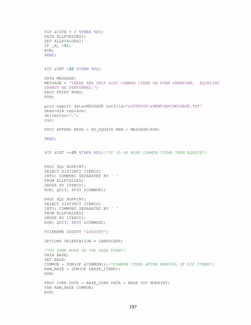
197

%IF &CIPE = Y %THEN %DO; DATA ALLPVALUES2; SET ALLPVALUES2; IF _N_ <51; RUN; %END; %IF &CNT <20 %THEN %DO; DATA MESSAGE; MESSAGE = "THERE ARE ONLY &CNT COMMON ITEMS ON FORM &NEWFORM. EQUATING CANNOT BE PERFORMED."; PROC PRINT NOBS; RUN; proc export data=MESSAGE outfile="&OUTPATH\&NEWFORM\MESSAGE.TXT" dbms=dlm replace; delimiter=","; run; PROC APPEND BASE = NO_EQUATE NEW = MESSAGE;RUN; %END; %IF &CNT >=20 %THEN %DO;/*IF 20 OR MORE COMMON ITEMS THEN EQUATE*/ PROC SQL NOPRINT; SELECT DISTINCT ITEMID1 INTO: COMMON1 SEPARATED BY ' ' FROM ALLPVALUES2 ORDER BY ITEMID1; RUN; QUIT; %PUT &COMMON1; PROC SQL NOPRINT; SELECT DISTINCT ITEMID1 INTO: COMMON2 SEPARATED BY ' ' FROM ALLPVALUES2 ORDER BY ITEMID1; RUN; QUIT; %PUT &COMMON2; FILENAME ODSOUT "&ODSOUT"; OPTIONS ORIENTATION = LANDSCAPE; /*DO SOME WORK ON THE BASE FORM*/ DATA BASE; SET BASE; COMMON = SUM(OF &COMMON1);/*COMMON ITEMS AFTER REMOVAL OF DIF ITEMS*/ RAW_BASE = SUM(OF &BASE_ITEMS); RUN; PROC CORR OUTP = BASE_CORR DATA = BASE COV NOPRINT; VAR RAW_BASE COMMON; RUN;

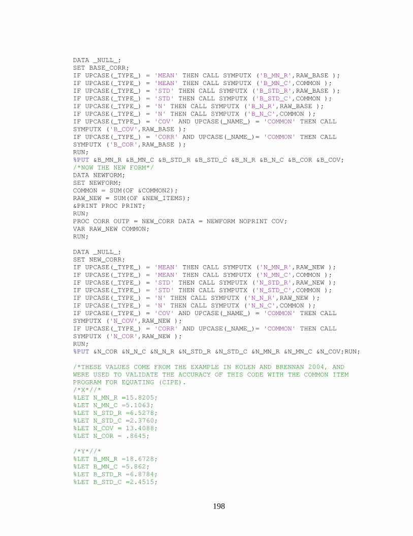
198

DATA _NULL_; SET BASE_CORR; IF UPCASE(_TYPE_) = 'MEAN' THEN CALL SYMPUTX ('B_MN_R',RAW_BASE ); IF UPCASE(_TYPE_) = 'MEAN' THEN CALL SYMPUTX ('B_MN_C',COMMON ); IF UPCASE(_TYPE_) = 'STD' THEN CALL SYMPUTX ('B_STD_R',RAW_BASE ); IF UPCASE(_TYPE_) = 'STD' THEN CALL SYMPUTX ('B_STD_C',COMMON ); IF UPCASE(_TYPE_) = 'N' THEN CALL SYMPUTX ('B_N_R',RAW_BASE ); IF UPCASE(_TYPE_) = 'N' THEN CALL SYMPUTX ('B_N_C',COMMON ); IF UPCASE(_TYPE_) = 'COV' AND UPCASE(_NAME_) = 'COMMON' THEN CALL SYMPUTX ('B_COV',RAW_BASE ); IF UPCASE(_TYPE_) = 'CORR' AND UPCASE(_NAME_)= 'COMMON' THEN CALL SYMPUTX ('B_COR',RAW_BASE ); RUN; %PUT &B_MN_R &B_MN_C &B_STD_R &B_STD_C &B_N_R &B_N_C &B_COR &B_COV; /*NOW THE NEW FORM*/ DATA NEWFORM; SET NEWFORM; COMMON = SUM(OF &COMMON2); RAW_NEW = SUM(OF &NEW_ITEMS); &PRINT PROC PRINT; RUN; PROC CORR OUTP = NEW_CORR DATA = NEWFORM NOPRINT COV; VAR RAW_NEW COMMON; RUN; DATA _NULL_; SET NEW_CORR; IF UPCASE(_TYPE_) = 'MEAN' THEN CALL SYMPUTX ('N_MN_R',RAW_NEW ); IF UPCASE(_TYPE_) = 'MEAN' THEN CALL SYMPUTX ('N_MN_C',COMMON ); IF UPCASE(_TYPE_) = 'STD' THEN CALL SYMPUTX ('N_STD_R',RAW_NEW ); IF UPCASE(_TYPE_) = 'STD' THEN CALL SYMPUTX ('N_STD_C',COMMON ); IF UPCASE(_TYPE_) = 'N' THEN CALL SYMPUTX ('N_N_R',RAW_NEW ); IF UPCASE(_TYPE_) = 'N' THEN CALL SYMPUTX ('N_N_C',COMMON ); IF UPCASE(_TYPE_) = 'COV' AND UPCASE(_NAME_) = 'COMMON' THEN CALL SYMPUTX ('N_COV',RAW_NEW ); IF UPCASE(_TYPE_) = 'CORR' AND UPCASE(_NAME_)= 'COMMON' THEN CALL SYMPUTX ('N_COR',RAW_NEW ); RUN; %PUT &N_COR &N_N_C &N_N_R &N_STD_R &N_STD_C &N_MN_R &N_MN_C &N_COV;RUN; /*THESE VALUES COME FROM THE EXAMPLE IN KOLEN AND BRENNAN 2004, AND WERE USED TO VALIDATE THE ACCURACY OF THIS CODE WITH THE COMMON ITEM PROGRAM FOR EQUATING (CIPE). /*X*//* %LET N_MN_R =15.8205; %LET N_MN_C =5.1063; %LET N_STD_R =6.5278; %LET N_STD_C =2.3760; %LET N_COV = 13.4088; %LET N_COR = .8645; /*Y*//* %LET B_MN_R =18.6728; %LET B_MN_C =5.862; %LET B_STD_R =6.8784; %LET B_STD_C =2.4515;

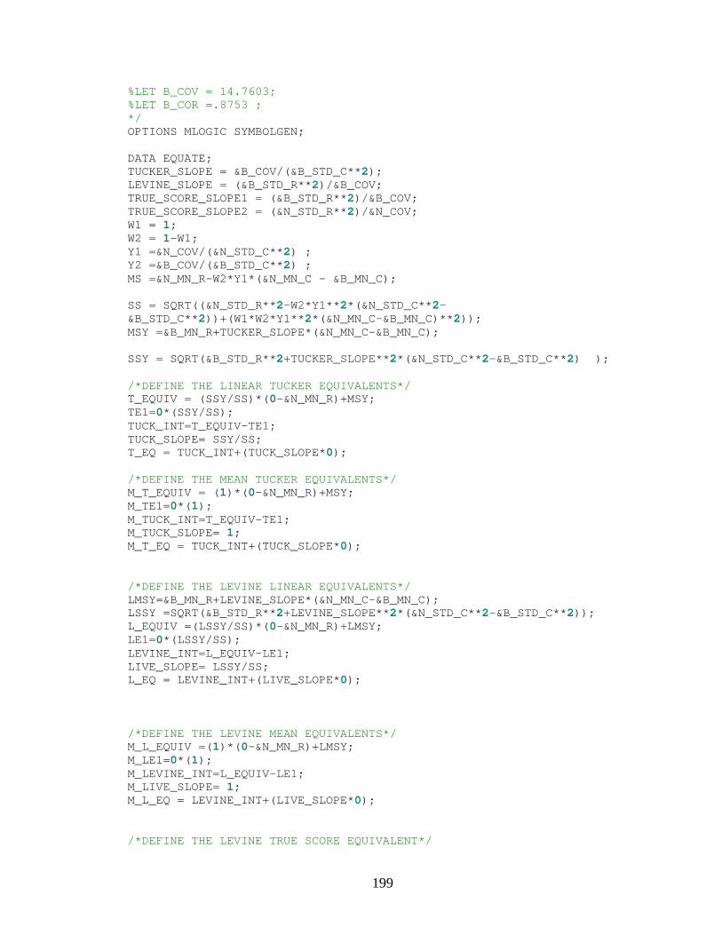
199

%LET B_COV = 14.7603; %LET B_COR =.8753 ; */ OPTIONS MLOGIC SYMBOLGEN; DATA EQUATE; TUCKER_SLOPE = &B_COV/(&B_STD_C**2); LEVINE_SLOPE = (&B_STD_R**2)/&B_COV; TRUE_SCORE_SLOPE1 = (&B_STD_R**2)/&B_COV; TRUE_SCORE_SLOPE2 = (&N_STD_R**2)/&N_COV; W1 = 1; W2 = 1-W1; Y1 =&N_COV/(&N_STD_C**2) ; Y2 =&B_COV/(&B_STD_C**2) ; MS =&N_MN_R-W2*Y1*(&N_MN_C - &B_MN_C); SS = SQRT((&N_STD_R**2-W2*Y1**2*(&N_STD_C**2-&B_STD_C**2))+(W1*W2*Y1**2*(&N_MN_C-&B_MN_C)**2)); MSY =&B_MN_R+TUCKER_SLOPE*(&N_MN_C-&B_MN_C); SSY = SQRT(&B_STD_R**2+TUCKER_SLOPE**2*(&N_STD_C**2-&B_STD_C**2) ); /*DEFINE THE LINEAR TUCKER EQUIVALENTS*/ T_EQUIV = (SSY/SS)*(0-&N_MN_R)+MSY; TE1=0*(SSY/SS); TUCK_INT=T_EQUIV-TE1; TUCK_SLOPE= SSY/SS; T_EQ = TUCK_INT+(TUCK_SLOPE*0); /*DEFINE THE MEAN TUCKER EQUIVALENTS*/ M_T_EQUIV = (1)*(0-&N_MN_R)+MSY; M_TE1=0*(1); M_TUCK_INT=T_EQUIV-TE1; M_TUCK_SLOPE= 1; M_T_EQ = TUCK_INT+(TUCK_SLOPE*0); /*DEFINE THE LEVINE LINEAR EQUIVALENTS*/ LMSY=&B_MN_R+LEVINE_SLOPE*(&N_MN_C-&B_MN_C); LSSY =SQRT(&B_STD_R**2+LEVINE_SLOPE**2*(&N_STD_C**2-&B_STD_C**2)); L_EQUIV =(LSSY/SS)*(0-&N_MN_R)+LMSY; LE1=0*(LSSY/SS); LEVINE_INT=L_EQUIV-LE1; LIVE_SLOPE= LSSY/SS; L_EQ = LEVINE_INT+(LIVE_SLOPE*0); /*DEFINE THE LEVINE MEAN EQUIVALENTS*/ M_L_EQUIV =(1)*(0-&N_MN_R)+LMSY; M_LE1=0*(1); M_LEVINE_INT=L_EQUIV-LE1; M_LIVE_SLOPE= 1; M_L_EQ = LEVINE_INT+(LIVE_SLOPE*0); /*DEFINE THE LEVINE TRUE SCORE EQUIVALENT*/

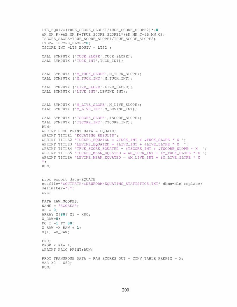
200

LTS_EQUIV=(TRUE_SCORE_SLOPE1/TRUE_SCORE_SLOPE2)*(0-&N_MN_R)+&B_MN_R+TRUE_SCORE_SLOPE1*(&N_MN_C-&B_MN_C); TSCORE_SLOPE=TRUE_SCORE_SLOPE1/TRUE_SCORE_SLOPE2; LTS2= TSCORE_SLOPE*0; TSCORE_INT =LTS_EQUIV - LTS2 ; CALL SYMPUTX ('TUCK_SLOPE',TUCK_SLOPE); CALL SYMPUTX ('TUCK_INT',TUCK_INT); CALL SYMPUTX ('M_TUCK_SLOPE',M_TUCK_SLOPE); CALL SYMPUTX ('M_TUCK_INT',M_TUCK_INT); CALL SYMPUTX ('LIVE_SLOPE',LIVE_SLOPE); CALL SYMPUTX ('LIVE_INT',LEVINE_INT); CALL SYMPUTX ('M_LIVE_SLOPE',M_LIVE_SLOPE); CALL SYMPUTX ('M_LIVE_INT',M_LEVINE_INT); CALL SYMPUTX ('TSCORE_SLOPE',TSCORE_SLOPE); CALL SYMPUTX ('TSCORE_INT',TSCORE_INT); RUN; &PRINT PROC PRINT DATA = EQUATE; &PRINT TITLE1 "EQUATING RESULTS"; &PRINT TITLE2 "TUCKER_EQUATED = &TUCK_INT + &TUCK_SLOPE * X "; &PRINT TITLE3 "LEVINE_EQUATED = &LIVE_INT + &LIVE_SLOPE * X "; &PRINT TITLE4 "TRUE_SCORE_EQUATED = &TSCORE_INT + &TSCORE_SLOPE * X "; &PRINT TITLE5 "TUCKER_MEAN_EQUATED = &M_TUCK_INT + &M_TUCK_SLOPE * X "; &PRINT TITLE6 "LEVINE_MEAN_EQUATED = &M_LIVE_INT + &M_LIVE_SLOPE * X "; RUN; proc export data=EQUATE outfile="&OUTPATH\&NEWFORM\EQUATING_STATISTICS.TXT" dbms=dlm replace; delimiter=","; run; DATA RAW_SCORES; NAME = "SCORES"; X0 = 0; ARRAY X[80] X1 - X80; X_RAW=0; DO I =1 TO 80; X_RAW =X_RAW + 1; X[I] =X_RAW; END; DROP X_RAW I; &PRINT PROC PRINT;RUN; PROC TRANSPOSE DATA = RAW_SCORES OUT = CONV_TABLE PREFIX = X; VAR X0 - X80; RUN;

201

/*CREATE THE LINEAR FORMULAS FOR THE CONVERSION TABLE*/ DATA CONV_TABLE; SET CONV_TABLE; TUCK_SCALE_INT=(&_B_+&_A_*(&TUCK_INT)); TUCK_SCALE_SLOPE=((&_A_*&TUCK_SLOPE)); M_TUCK_SCALE_INT=(&_B_+&_A_*(&M_TUCK_INT)); M_TUCK_SCALE_SLOPE=((&_A_*&M_TUCK_SLOPE)); LIVE_SCALE_INT=(&_B_+&_A_*(&LIVE_INT)); LIVE_SCALE_SLOPE=((&_A_*&LIVE_SLOPE)); M_LIVE_SCALE_INT=(&_B_+&_A_*(&M_LIVE_INT)); M_LIVE_SCALE_SLOPE=((&_A_*&M_LIVE_SLOPE)); TSCORE_SCALE_INT=(&_B_+&_A_*(&TSCORE_INT)); TSCORE_SCALE_SLOPE=((&_A_*&TSCORE_SLOPE)); TUCK_SCALE_SCORE=(X1*TUCK_SCALE_SLOPE)+TUCK_SCALE_INT; LIVE_SCALE_SCORE=(X1*LIVE_SCALE_SLOPE)+LIVE_SCALE_INT; TSCORE_SCALE_SCORE=(X1*TSCORE_SCALE_SLOPE)+TSCORE_SCALE_INT; &print proc print; &print WHERE X1 = 1; &print VAR TUCK_SCALE_INT TUCK_SCALE_SLOPE LIVE_SCALE_INT LIVE_SCALE_SLOPE TSCORE_SCALE_INT TSCORE_SCALE_SLOPE; RUN; /*CREATE THE LINEAR FORMULAS FOR THE CONVERSION TABLE*/ DATA CONV_TABLE; SET CONV_TABLE; RENAME X1 =&NEWFORM;/*THE EQUIVALENT IS THE ESTIMATED BASE*/ TUCK_SCALE_INT=(&_B_+&_A_*(&TUCK_INT)); TUCK_SCALE_SLOPE=((&_A_*&TUCK_SLOPE)); M_TUCK_SCALE_INT=(&_B_+&_A_*(&M_TUCK_INT)); M_TUCK_SCALE_SLOPE=((&_A_*&M_TUCK_SLOPE)); LIVE_SCALE_INT=(&_B_+&_A_*(&LIVE_INT)); LIVE_SCALE_SLOPE=((&_A_*&LIVE_SLOPE)); M_LIVE_SCALE_INT=(&_B_+&_A_*(&M_LIVE_INT)); M_LIVE_SCALE_SLOPE=((&_A_*&M_LIVE_SLOPE)); TSCORE_SCALE_INT=(&_B_+&_A_*(&TSCORE_INT)); TSCORE_SCALE_SLOPE=((&_A_*&TSCORE_SLOPE)); TUCK_SCALE_SCORE=(X1*TUCK_SCALE_SLOPE)+TUCK_SCALE_INT; LIVE_SCALE_SCORE=(X1*LIVE_SCALE_SLOPE)+LIVE_SCALE_INT; TSCORE_SCALE_SCORE=(X1*TSCORE_SCALE_SLOPE)+TSCORE_SCALE_INT; M_TUCK_SCALE_SCORE=(X1*M_TUCK_SCALE_SLOPE)+M_TUCK_SCALE_INT; M_LIVE_SCALE_SCORE=(X1*M_LIVE_SCALE_SLOPE)+M_LIVE_SCALE_INT;

202

RNDED_TUCKSS =ROUND(TUCK_SCALE_SCORE,1); RNDED_LEVSS =ROUND(LIVE_SCALE_SCORE,1); RNDED_TRUESS =ROUND(TSCORE_SCALE_SCORE,1); M_RNDED_TUCKSS =ROUND(M_TUCK_SCALE_SCORE,1); M_RNDED_LEVSS =ROUND(M_LIVE_SCALE_SCORE,1); RUN; proc export data=CONV_TABLE outfile="&OUTPATH\&NEWFORM\CONVERSION_TABLE.TXT" dbms=dlm replace; delimiter=","; run; /*CALCULATE THE PERCENT PASSING ACCORDING TO EACH EQUATING METHOD*/ %LET TUCKSS_CUT = 0; %LET LEVSS_CUT = 0; %LET TRUESS_CUT = 0; DATA TUCK (KEEP=RNDED_TUCKSS TUCK_SCALE_INT TUCK_SCALE_SLOPE &NEWFORM) LEV (KEEP=RNDED_LEVSS LIVE_SCALE_INT LIVE_SCALE_SLOPE &NEWFORM) TS (KEEP=RNDED_TRUESS TSCORE_SCALE_INT TSCORE_SCALE_SLOPE &NEWFORM); SET CONV_TABLE; IF RNDED_TUCKSS = 75 THEN OUTPUT TUCK ; IF RNDED_LEVSS = 75 THEN OUTPUT LEV; IF RNDED_TRUESS = 75 THEN OUTPUT TS; IF RNDED_TUCKSS = 75 THEN CALL SYMPUTX ('TUCKSS_CUT ', &NEWFORM ); IF RNDED_LEVSS = 75 THEN CALL SYMPUTX ('LEVSS_CUT', &NEWFORM ); IF RNDED_TRUESS = 75 THEN CALL SYMPUTX ('TRUESS_CUT ', &NEWFORM ); RUN; /*FIGURE THE PERCENT PASSING*/ DATA PASSES; SET NEWFORM; TUCKSS_CUT = &TUCKSS_CUT ; LEVSS_CUT=&LEVSS_CUT; TRUESS_CUT=&TRUESS_CUT; TUCKER_PASS = 0; IF RAW_SCORE => TUCKSS_CUT THEN TUCKER_PASS = 1; LEVINE_PASS = 0; IF RAW_SCORE => LEVSS_CUT THEN LEVINE_PASS = 1; TSCORE_PASS = 0; IF RAW_SCORE => TRUESS_CUT THEN TSCORE_PASS = 1; IDENTITY_PASS = 0; IF RAW_SCORE => 55 THEN IDENTITY_PASS = 1;

203

KEEP CANDIDATEID RAWSCORE2 TSCORE_PASS LEVINE_PASS TUCKER_PASS IDENTITY_PASS; RUN; proc export data=PASSES outfile="&OUTPATH\&NEWFORM\PASS_FAIL.TXT" dbms=dlm replace; delimiter=","; run; PROC FREQ DATA = PASSES ;TABLE IDENTITY_PASS/OUT= IDENTITY_PASS;RUN; PROC FREQ DATA = PASSES ;TABLE LEVINE_PASS/OUT= LEVINE_PASS;RUN; PROC FREQ DATA = PASSES ;TABLE TUCKER_PASS/OUT= TUCKER_PASS;RUN; PROC FREQ DATA = PASSES ;TABLE TSCORE_PASS/OUT= TSCORE_PASS;RUN; DATA _NULL_;SET IDENTITY_PASS;IF IDENTITY_PASS = 1 THEN CALL SYMPUTX ('IDENT_PASS ',PERCENT );RUN; %PUT &IDENT_PASS; DATA _NULL_;SET LEVINE_PASS;IF LEVINE_PASS = 1 THEN CALL SYMPUTX ('LEVINE_PASS ',PERCENT );RUN; %PUT &IDENT_PASS; DATA _NULL_;SET TUCKER_PASS;IF TUCKER_PASS = 1 THEN CALL SYMPUTX ('TUCKER_PASS ',PERCENT );RUN; %PUT &IDENT_PASS; DATA _NULL_;SET TSCORE_PASS;IF TSCORE_PASS = 1 THEN CALL SYMPUTX ('TSCORE_PASS ',PERCENT );RUN; %PUT &IDENT_PASS; DATA TUCK; SET TUCK; PASS = &TUCKER_pASS; RENAME TUCK_SCALE_INT = INTERCEPT TUCK_SCALE_SLOPE = SLOPE RNDED_TUCKSS = SCALE_SCORE; METHOD = "TUCKER "; RUN; DATA LEV; SET LEV; PASS = &LEVINE_PASS; RENAME LIVE_SCALE_INT = INTERCEPT LIVE_SCALE_SLOPE = SLOPE RNDED_LEVSS = SCALE_SCORE; METHOD = "LEVINE "; RUN; DATA TS; SET TS; PASS = &TSCORE_pASS; RENAME TSCORE_SCALE_INT = INTERCEPT TSCORE_SCALE_SLOPE = SLOPE RNDED_TRUESS = SCALE_SCORE; METHOD = "TRUE_SCORE "; RUN; DATA _NULL_; SET ALLPVALUES2; CALL SYMPUTX ('COMMON_REMAINING', _N_ ); RUN; DATA SUMMARY;

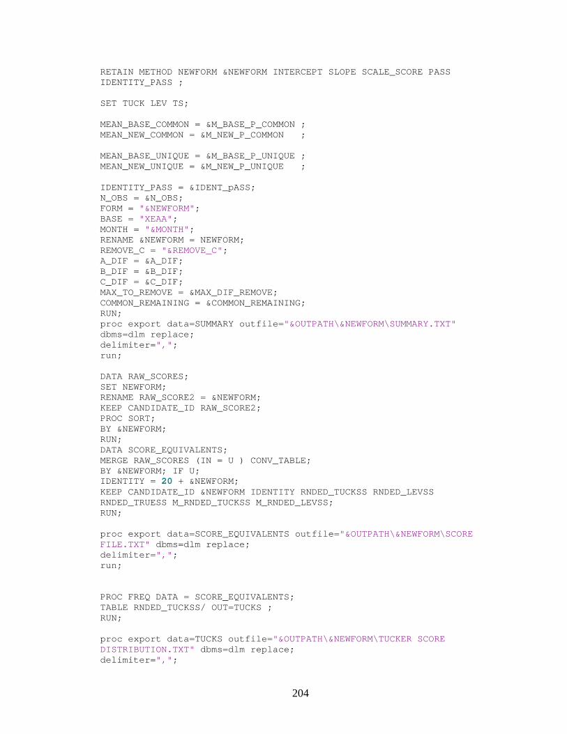
204

RETAIN METHOD NEWFORM &NEWFORM INTERCEPT SLOPE SCALE_SCORE PASS IDENTITY_PASS ; SET TUCK LEV TS; MEAN_BASE_COMMON = &M_BASE_P_COMMON ; MEAN_NEW_COMMON = &M_NEW_P_COMMON ; MEAN_BASE_UNIQUE = &M_BASE_P_UNIQUE ; MEAN_NEW_UNIQUE = &M_NEW_P_UNIQUE ; IDENTITY_PASS = &IDENT_pASS; N_OBS = &N_OBS; FORM = "&NEWFORM"; BASE = "XEAA"; MONTH = "&MONTH"; RENAME &NEWFORM = NEWFORM; REMOVE_C = "&REMOVE_C"; A_DIF = &A_DIF; B_DIF = &B_DIF; C_DIF = &C_DIF; MAX_TO_REMOVE = &MAX_DIF_REMOVE; COMMON_REMAINING = &COMMON_REMAINING; RUN; proc export data=SUMMARY outfile="&OUTPATH\&NEWFORM\SUMMARY.TXT" dbms=dlm replace; delimiter=","; run; DATA RAW_SCORES; SET NEWFORM; RENAME RAW_SCORE2 = &NEWFORM; KEEP CANDIDATE_ID RAW_SCORE2; PROC SORT; BY &NEWFORM; RUN; DATA SCORE_EQUIVALENTS; MERGE RAW_SCORES (IN = U ) CONV_TABLE; BY &NEWFORM; IF U; IDENTITY = 20 + &NEWFORM; KEEP CANDIDATE_ID &NEWFORM IDENTITY RNDED_TUCKSS RNDED_LEVSS RNDED_TRUESS M_RNDED_TUCKSS M_RNDED_LEVSS; RUN; proc export data=SCORE_EQUIVALENTS outfile="&OUTPATH\&NEWFORM\SCORE FILE.TXT" dbms=dlm replace; delimiter=","; run; PROC FREQ DATA = SCORE_EQUIVALENTS; TABLE RNDED_TUCKSS/ OUT=TUCKS ; RUN; proc export data=TUCKS outfile="&OUTPATH\&NEWFORM\TUCKER SCORE DISTRIBUTION.TXT" dbms=dlm replace; delimiter=",";

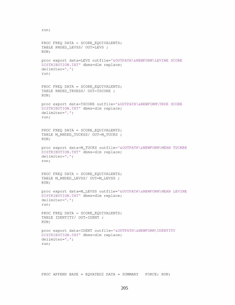
205

run; PROC FREQ DATA = SCORE_EQUIVALENTS; TABLE RNDED_LEVSS/ OUT=LEVS ; RUN; proc export data=LEVS outfile="&OUTPATH\&NEWFORM\LEVINE SCORE DISTRIBUTION.TXT" dbms=dlm replace; delimiter=","; run; PROC FREQ DATA = SCORE_EQUIVALENTS; TABLE RNDED_TRUESS/ OUT=TSCORE ; RUN; proc export data=TSCORE outfile="&OUTPATH\&NEWFORM\TRUE SCORE DISTRIBUTION.TXT" dbms=dlm replace; delimiter=","; run; PROC FREQ DATA = SCORE_EQUIVALENTS; TABLE M_RNDED_TUCKSS/ OUT=M_TUCKS ; RUN; proc export data=M_TUCKS outfile="&OUTPATH\&NEWFORM\MEAN TUCKER DISTRIBUTION.TXT" dbms=dlm replace; delimiter=","; run; PROC FREQ DATA = SCORE_EQUIVALENTS; TABLE M_RNDED_LEVSS/ OUT=M_LEVSS ; RUN; proc export data=M_LEVSS outfile="&OUTPATH\&NEWFORM\MEAN LEVINE DISTRIBUTION.TXT" dbms=dlm replace; delimiter=","; run; PROC FREQ DATA = SCORE_EQUIVALENTS; TABLE IDENTITY/ OUT=IDENT ; RUN; proc export data=IDENT outfile="&OUTPATH\&NEWFORM\IDENTITY DISTRIBUTION.TXT" dbms=dlm replace; delimiter=","; run; PROC APPEND BASE = EQUATED2 DATA = SUMMARY FORCE; RUN;

206

%END; PROC SORT DATA =EQUATED2; BY METHOD FORM;RUN; PROC PRINT DATA= EQUATED2; TITLE "EQUATED FORMS "; RUN; PROC PRINT DATA =NO_EQUATE; TITLE "FORMS NOT EQUATED"; RUN; PROC DATASETS; SAVE t_b LIST EQUATED2 NO_EQUATE; QUIT; RUN; %MEND;

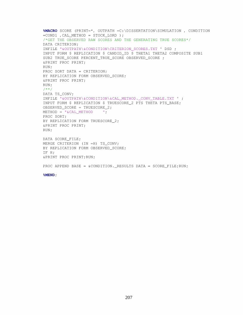
207

%MACRO SCORE (PRINT=*, OUTPATH =C:\DISSERTATION\SIMULATION , CONDITION =COND1 ,CAL_METHOD = STOCK_LORD ); /*GET THE OBSERVED RAW SCORES AND THE GENERATING TRUE SCORES*/ DATA CRITERION; INFILE "&OUTPATH\&CONDITION\CRITERION_SCORES.TXT " DSD ; INPUT FORM $ REPLICATION $ CANDID_ID $ THETA1 THETA2 COMPOSITE SUB1 SUB2 TRUE_SCORE PERCENT_TRUE_SCORE OBSERVED_SCORE ; &PRINT PROC PRINT; RUN; PROC SORT DATA = CRITERION; BY REPLICATION FORM OBSERVED_SCORE; &PRINT PROC PRINT; RUN; /**/ DATA TS_CONV; INFILE "&OUTPATH\&CONDITION\&CAL_METHOD._CONV_TABLE.TXT " ; INPUT FORM $ REPLICATION $ TRUESCORE_2 PTS THETA PTS_BASE; OBSERVED_SCORE = TRUESCORE_2; METHOD = "&CAL_METHOD "; PROC SORT; BY REPLICATION FORM TRUESCORE_2; &PRINT PROC PRINT; RUN; DATA SCORE_FILE; MERGE CRITERION (IN =H) TS_CONV; BY REPLICATION FORM OBSERVED_SCORE; IF H; &PRINT PROC PRINT;RUN; PROC APPEND BASE = &CONDITION._RESULTS DATA = SCORE_FILE;RUN; %MEND;

208

%MACRO EQUIP (PRINT=*,OUTPATH = C:DISSERTATION\SIMULATION, CONDITION = COND1, FORM = B , ADMIN = 2, OUTPATH =C:\DISSERTATION\SIMULATION); DATA POPX; INFILE "&OUTPATH\&CONDITION\POPULATION X.TXT" DSD; INPUT CANDID $ X1 X2; RUN; DATA POPY; INFILE "&OUTPATH\&CONDITION\POPULATION Y.TXT" DSD; INPUT CANDID $ Y1 Y2; RUN; DATA DAT; SET POPX POPY; RUN; DATA DAT; SET DAT; X1 = ROUND(X1,.1); X2 = ROUND(X2,.1); Y1 = ROUND(Y1,.1); Y2 = ROUND(Y2,.1); &PRINT PROC PRINT; &PRINT VAR X1 X2 Y1 Y2;RUN; RUN; PROC FREQ DATA = DAT NOPRINT; TABLE X1 / OUT =OUT1; RUN; PROC FREQ DATA = DAT NOPRINT; TABLE X2 / OUT =OUT2; RUN; PROC FREQ DATA = DAT NOPRINT; TABLE Y1 / OUT =OUT3; RUN; PROC FREQ DATA = DAT NOPRINT; TABLE Y2 / OUT =OUT4; RUN; DATA OUT1; SET OUT1; RENAME X1 = VALUE; THETA = 1; RUN; DATA OUT2; SET OUT2; RENAME X2 = VALUE; THETA = 2; RUN; DATA OUT3; SET OUT3; RENAME Y1 = VALUE;

209

THETA = 3; RUN; DATA OUT4; SET OUT4; RENAME Y2 = VALUE; THETA = 4; RUN; DATA ALLTHETAS; SET OUT1 OUT2 OUT3 OUT4; IF PERCENT = . THEN DELETE; &PRINT PROC PRINT;RUN; DATA FORMA; INFILE "C:\DISSERTATION\SIMULATION\&CONDITION\FREQ_A.TXT" DSD ; INPUT SCORE COUNT PERCENT NITEMS ; FORM ="FORM_A"; &PRINT PROC PRINT; RUN; DATA FORM&FORM; INFILE "C:\DISSERTATION\SIMULATION\&CONDITION\FREQ_&FORM..TXT" DSD ; INPUT SCORE COUNT PERCENT NITEMS ; FORM ="FORM_&FORM"; &PRINT PROC PRINT; RUN; DATA BOTH_TS; SET FORMA FORM&FORM; &PRINT PROC PRINT; RUN; &PRINT PROC PRINT DATA = BOTH;RUN; DATA TEMP122; SET BOTH_TS; PROC SORT DATA = TEMP122; BY DESCENDING COUNT; RUN; DATA _NULL_; SET TEMP122; COUNT = COUNT + 200; IF _N_ = 1 THEN CALL SYMPUTX ('MAX_CNT',COUNT ); RUN; %MEND; %MACRO MAKE_TCC (PRINT=*, N_REPS=50,CAL_METHOD = FPC, OUTPATH =C:\DISSERTATION\SIMULATION,REPLICATION = REP1, CONDITION = COND, FORM2=B, FORM1=A );

210

%DO R = 1 %TO &N_REPS; proc import datafile="&OUTPATH\&CONDITION\REP&R\CONV_TABLES\FPC_CONV_TABLE_&FORM2..TXT" out=FPC&FORM2 dbms=csv replace; getnames=YES; run; proc import datafile="&OUTPATH\&CONDITION\REP&R\CONV_TABLES\STOCK_LORD_CONV_TABLE_&FORM2..TXT" out=SL&FORM2 dbms=csv replace; getnames=YES; run; DATA FPC&FORM2; SET FPC&FORM2; METHOD = "FPC_"; RUN; DATA SL&FORM2; SET SL&FORM2; METHOD = "SCSL"; RUN; DATA &FORM2; SET FPC&FORM2 SL&FORM2; RUN; DATA &FORM1; SET &FORM2; RAWSCORE=TRUESCORE_1; FORM = "&FORM1"; REP ="&REPLICATION"; KEEP RAWSCORE THETA FORM REP METHOD; RUN; DATA &FORM2; SET &FORM2; RAWSCORE= TRUESCORE_2 ; FORM = "&FORM2"; REP ="&REPLICATION"; KEEP RAWSCORE THETA FORM REP METHOD; RUN; DATA BOTH&FORM2._&R; SET &FORM1 &FORM2 ; IF THETA > 4 THEN THETA = 4; IF THETA <-4 THEN THETA = -4; &PRINT PROC PRINT;RUN; %IF &N_REPS = 1 %THEN %DO; DATA NEW&FORM2; SET BOTH&FORM2._&R; RUN;

211

%END; %ELSE %DO; DATA NEW&FORM2; SET NEW&FORM2 BOTH&FORM2._&R; RUN; %END; %END; &PRINT PROC PRINT DATA = NEWB;RUN; DATA NEW&FORM2; SET NEW&FORM2; METHOD2 = COMPRESS(METHOD||"_"||FORM); THETA = ROUND(THETA,.1); RAWSCORE = ROUND(RAWSCORE,1); RUN; PROC MEANS DATA = NEW&FORM2 NOPRINT; CLASS METHOD2 FORM RAWSCORE ; VAR THETA; OUTPUT OUT = ALLMEANS&FORM2 MEAN = ; RUN; DATA SCSLALLMEANS&FORM2 FPCALLMEANS&FORM2; SET ALLMEANS&FORM2; IF FORM NE " "; IF METHOD2 NE " "; METHOD_ = COMPRESS("FORM_"||SUBSTRN(METHOD2,6,1)); IF METHOD2 EQ "SCSL_A" THEN OUTPUT SCSLALLMEANS&FORM2; IF METHOD2 EQ "SCSL_B" THEN OUTPUT SCSLALLMEANS&FORM2; IF METHOD2 EQ "FPC__A" THEN OUTPUT FPCALLMEANS&FORM2; IF METHOD2 EQ "FPC__B" THEN OUTPUT FPCALLMEANS&FORM2; IF METHOD2 EQ "SCSL_C" THEN OUTPUT SCSLALLMEANS&FORM2; IF METHOD2 EQ "SCSL_D" THEN OUTPUT SCSLALLMEANS&FORM2; IF METHOD2 EQ "FPC__C" THEN OUTPUT FPCALLMEANS&FORM2; IF METHOD2 EQ "FPC__D" THEN OUTPUT FPCALLMEANS&FORM2; IF METHOD2 EQ "SCSL_E" THEN OUTPUT SCSLALLMEANS&FORM2; IF METHOD2 EQ "FPC__E" THEN OUTPUT FPCALLMEANS&FORM2; IF _TYPE_ EQ 7; &PRINT PROC PRINT; RUN; %MEND;

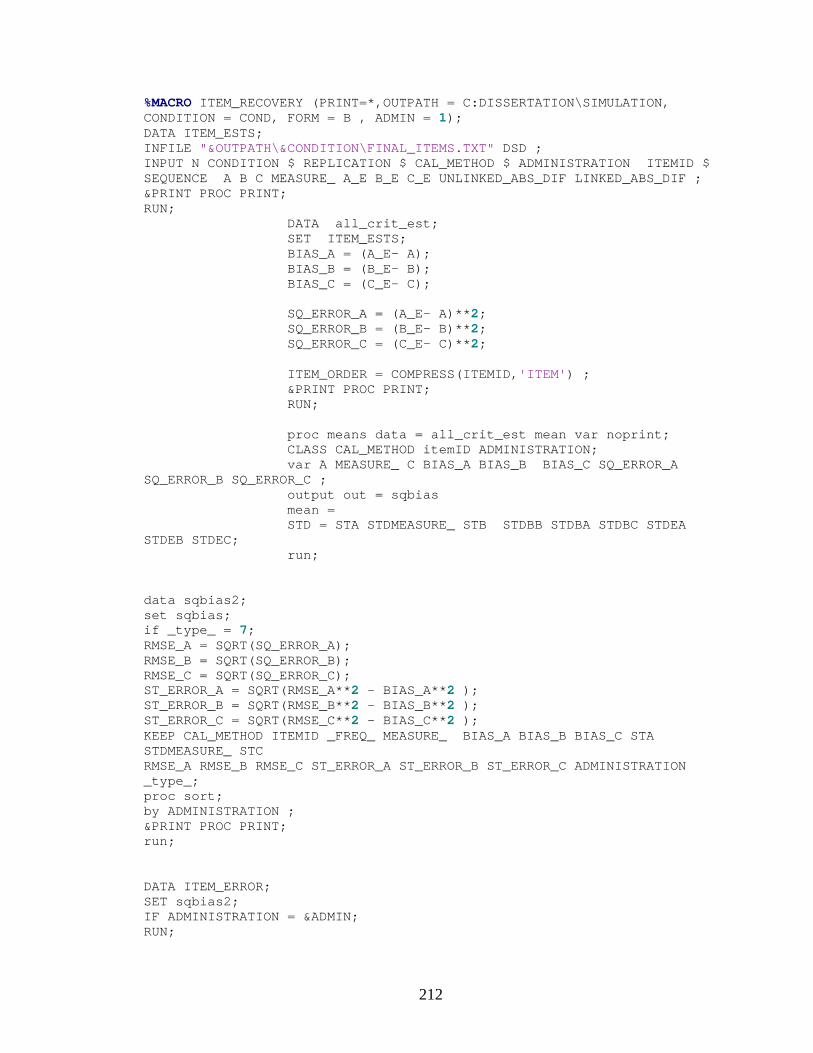
212

%MACRO ITEM_RECOVERY (PRINT=*,OUTPATH = C:DISSERTATION\SIMULATION, CONDITION = COND, FORM = B , ADMIN = 1); DATA ITEM_ESTS; INFILE "&OUTPATH\&CONDITION\FINAL_ITEMS.TXT" DSD ; INPUT N CONDITION $ REPLICATION $ CAL_METHOD $ ADMINISTRATION ITEMID $ SEQUENCE A B C MEASURE_ A_E B_E C_E UNLINKED_ABS_DIF LINKED_ABS_DIF ; &PRINT PROC PRINT; RUN; DATA all_crit_est; SET ITEM_ESTS; BIAS_A = (A_E- A); BIAS_B = (B_E- B); BIAS_C = (C_E- C); SQ_ERROR_A = (A_E- A)**2; SQ_ERROR_B = (B_E- B)**2; SQ_ERROR_C = (C_E- C)**2; ITEM_ORDER = COMPRESS(ITEMID,'ITEM') ; &PRINT PROC PRINT; RUN; proc means data = all_crit_est mean var noprint; CLASS CAL_METHOD itemID ADMINISTRATION; var A MEASURE_ C BIAS_A BIAS_B BIAS_C SQ_ERROR_A SQ_ERROR_B SQ_ERROR_C ; output out = sqbias mean = STD = STA STDMEASURE_ STB STDBB STDBA STDBC STDEA STDEB STDEC; run; data sqbias2; set sqbias; if _type_ = 7; RMSE_A = SQRT(SQ_ERROR_A); RMSE_B = SQRT(SQ_ERROR_B); RMSE_C = SQRT(SQ_ERROR_C); ST_ERROR_A = SQRT(RMSE_A**2 - BIAS_A**2 ); ST_ERROR_B = SQRT(RMSE_B**2 - BIAS_B**2 ); ST_ERROR_C = SQRT(RMSE_C**2 - BIAS_C**2 ); KEEP CAL_METHOD ITEMID _FREQ_ MEASURE_ BIAS_A BIAS_B BIAS_C STA STDMEASURE_ STC RMSE_A RMSE_B RMSE_C ST_ERROR_A ST_ERROR_B ST_ERROR_C ADMINISTRATION _type_; proc sort; by ADMINISTRATION ; &PRINT PROC PRINT; run; DATA ITEM_ERROR; SET sqbias2; IF ADMINISTRATION = &ADMIN; RUN;

213

PROC SORT DATA = ITEM_ERROR; BY CAL_METHOD;RUN; DATA ITEM_ERROR; SET ITEM_ERROR; BY CAL_METHOD; ITEM +1; IF FIRST.CAL_METHOD THEN DO; ITEM =1; END; IF CAL_METHOD = "STOCK_LO" THEN METHOD = "SCSL"; IF CAL_METHOD = "FPC" THEN METHOD = "FPC_"; RUN; %MEND;

214

%MACRO COLLECT_COMMON ( PRINT =, CAL_METHOD = STOCK_LORD, OLD_ADMIN = 1,/*USED FOR SELECTION*/ OLD_FORM = A,/*LABELING ONLY*/ NEW_ADMIN = 2,/*USED FOR SELECTION*/ NEW_FORM = B,/*LABELING ONLY*/ OUTPATH =C:\DISSERTATION\SIMULATION, CONDITION = CONDITION_7, END = 50 ); %DO I = 1 %TO &END; DATA ITEM_ESTS1_&I; INFILE "&OUTPATH\&CONDITION\REP&I\ADMIN&OLD_ADMIN\&CAL_METHOD\FINAL_ITEMS.TXT" DSD ; INPUT ITEMID $ ORDER A B C EST_B LINKED_A LINKED_B LINKED_C ERROR1 ERROR2; ADMINISTRATION = "ADMIN1"; FORM = "&OLD_FORM"; RUN; DATA ITEM_ESTS2_&I; INFILE "&OUTPATH\&CONDITION\REP&I\ADMIN&NEW_ADMIN\&CAL_METHOD\FINAL_ITEMS.TXT" DSD ; INPUT ITEMID $ ORDER A B C EST_B LINKED_A LINKED_B LINKED_C ERROR1 ERROR2; ADMINISTRATION = "ADMIN&NEW_ADMIN"; FORM = "&NEW_FORM"; RUN; %IF I = 1 %THEN %DO; DATA ALL_COMMON; SET ITEM_ESTS1_&I ITEM_ESTS2_&I; RUN; %END; %IF I >1 %THEN %DO; DATA ALL_COMMON; SET ALL_COMMON ITEM_ESTS1_&I ITEM_ESTS2_&I; RUN; %END; %END; DATA ALL_COMMON; SET ALL_COMMON; COMMON = "COMMON &OLD_FORM &NEW_FORM"; RUN; PROC MEANS DATA = ALL_COMMON NOPRINT; CLASS FORM ITEMID;

215

VAR A B LINKED_A lINKED_B EST_B; OUTPUT OUT = ALL_COMM_MEANS MEAN =; RUN; DATA ALL_COMM_MEANS; SET ALL_COMM_MEANS; IF _TYPE_ = 3; RUN; DATA &OLD_FORM &NEW_FORM; SET ALL_COMM_MEANS; IF FORM = "&OLD_FORM " THEN OUTPUT &OLD_FORM; IF FORM = "&NEW_FORM " THEN OUTPUT &NEW_FORM; KEEP ITEMID FORM LINKED_B LINKED_A; RUN; PROC SORT DATA = &OLD_FORM; BY ITEMID; PROC SORT DATA = &NEW_FORM; BY ITEMID; RUN; DATA &OLD_FORM; SET &OLD_FORM; RENAME LINKED_B = BASE_B LINKED_A = BASE_A FORM = BASE_FORM; RUN; DATA COMMON_SIDE_BY_SIDE; MERGE &OLD_FORM (IN=J) &NEW_FORM (IN=H); BY ITEMID; IF H; IF J; RUN; %MEND;

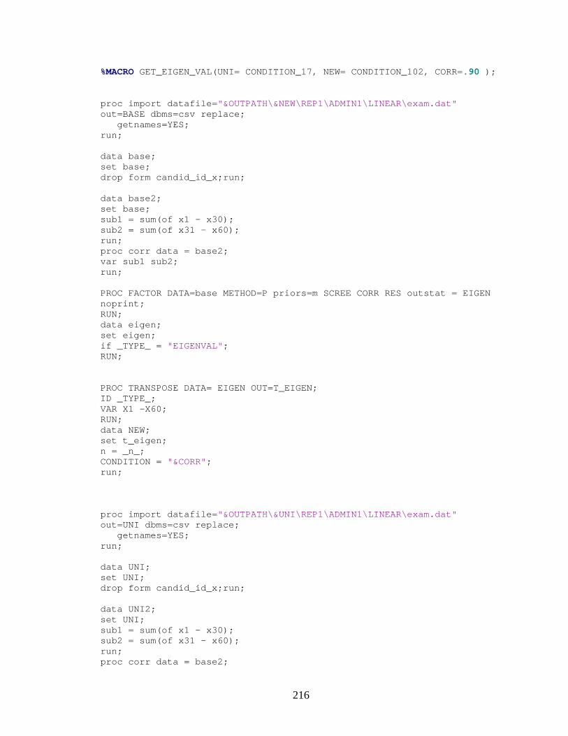
216

%MACRO GET_EIGEN_VAL(UNI= CONDITION_17, NEW= CONDITION_102, CORR=.90 ); proc import datafile="&OUTPATH\&NEW\REP1\ADMIN1\LINEAR\exam.dat" out=BASE dbms=csv replace; getnames=YES; run; data base; set base; drop form candid_id_x;run; data base2; set base; sub1 = sum(of x1 - x30); sub2 = sum(of x31 - x60); run; proc corr data = base2; var sub1 sub2; run; PROC FACTOR DATA=base METHOD=P priors=m SCREE CORR RES outstat = EIGEN noprint; RUN; data eigen; set eigen; if _TYPE_ = "EIGENVAL"; RUN; PROC TRANSPOSE DATA= EIGEN OUT=T_EIGEN; ID _TYPE_; VAR X1 -X60; RUN; data NEW; set t_eigen; n = _n_; CONDITION = "&CORR"; run; proc import datafile="&OUTPATH\&UNI\REP1\ADMIN1\LINEAR\exam.dat" out=UNI dbms=csv replace; getnames=YES; run; data UNI; set UNI; drop form candid_id_x;run; data UNI2; set UNI; sub1 = sum(of x1 - x30); sub2 = sum(of x31 - x60); run; proc corr data = base2;

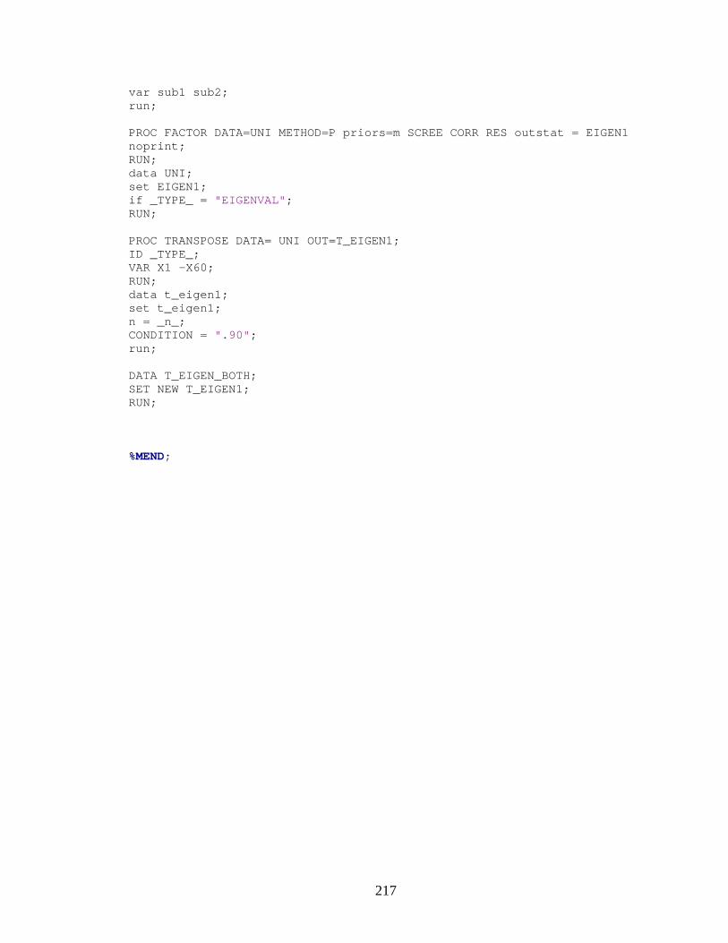
217

var sub1 sub2; run; PROC FACTOR DATA=UNI METHOD=P priors=m SCREE CORR RES outstat = EIGEN1 noprint; RUN; data UNI; set EIGEN1; if _TYPE_ = "EIGENVAL"; RUN; PROC TRANSPOSE DATA= UNI OUT=T_EIGEN1; ID _TYPE_; VAR X1 -X60; RUN; data t_eigen1; set t_eigen1; n = _n_; CONDITION = ".90"; run; DATA T_EIGEN_BOTH; SET NEW T_EIGEN1; RUN; %MEND;

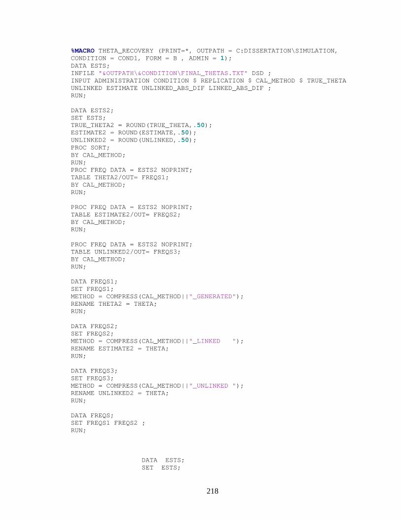
218

%MACRO THETA_RECOVERY (PRINT=*, OUTPATH = C:DISSERTATION\SIMULATION, CONDITION = COND1, FORM = B , ADMIN = 1); DATA ESTS; INFILE "&OUTPATH\&CONDITION\FINAL_THETAS.TXT" DSD ; INPUT ADMINISTRATION CONDITION $ REPLICATION $ CAL_METHOD $ TRUE_THETA UNLINKED ESTIMATE UNLINKED_ABS_DIF LINKED_ABS_DIF ; RUN; DATA ESTS2; SET ESTS; TRUE_THETA2 = ROUND(TRUE_THETA,.50); ESTIMATE2 = ROUND(ESTIMATE,.50); UNLINKED2 = ROUND(UNLINKED,.50); PROC SORT; BY CAL_METHOD; RUN; PROC FREQ DATA = ESTS2 NOPRINT; TABLE THETA2/OUT= FREQS1; BY CAL_METHOD; RUN; PROC FREQ DATA = ESTS2 NOPRINT; TABLE ESTIMATE2/OUT= FREQS2; BY CAL_METHOD; RUN; PROC FREQ DATA = ESTS2 NOPRINT; TABLE UNLINKED2/OUT= FREQS3; BY CAL_METHOD; RUN; DATA FREQS1; SET FREQS1; METHOD = COMPRESS(CAL_METHOD||"_GENERATED"); RENAME THETA2 = THETA; RUN; DATA FREQS2; SET FREQS2; METHOD = COMPRESS(CAL_METHOD||"_LINKED "); RENAME ESTIMATE2 = THETA; RUN; DATA FREQS3; SET FREQS3; METHOD = COMPRESS(CAL_METHOD||"_UNLINKED "); RENAME UNLINKED2 = THETA; RUN; DATA FREQS; SET FREQS1 FREQS2 ; RUN; DATA ESTS; SET ESTS;

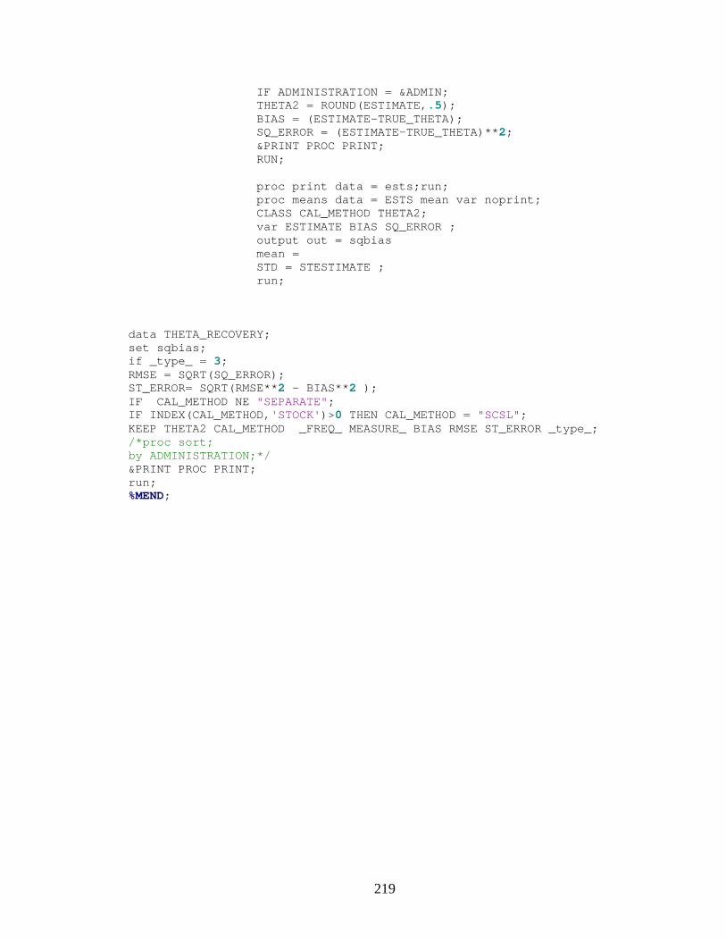
219

IF ADMINISTRATION = &ADMIN; THETA2 = ROUND(ESTIMATE,.5); BIAS = (ESTIMATE-TRUE_THETA); SQ_ERROR = (ESTIMATE-TRUE_THETA)**2; &PRINT PROC PRINT; RUN; proc print data = ests;run; proc means data = ESTS mean var noprint; CLASS CAL_METHOD THETA2; var ESTIMATE BIAS SQ_ERROR ; output out = sqbias mean = STD = STESTIMATE ; run; data THETA_RECOVERY; set sqbias; if _type_ = 3; RMSE = SQRT(SQ_ERROR); ST_ERROR= SQRT(RMSE**2 - BIAS**2 ); IF CAL_METHOD NE "SEPARATE"; IF INDEX(CAL_METHOD,'STOCK')>0 THEN CAL_METHOD = "SCSL"; KEEP THETA2 CAL_METHOD _FREQ_ MEASURE_ BIAS RMSE ST_ERROR _type_; /*proc sort; by ADMINISTRATION;*/ &PRINT PROC PRINT; run; %MEND;

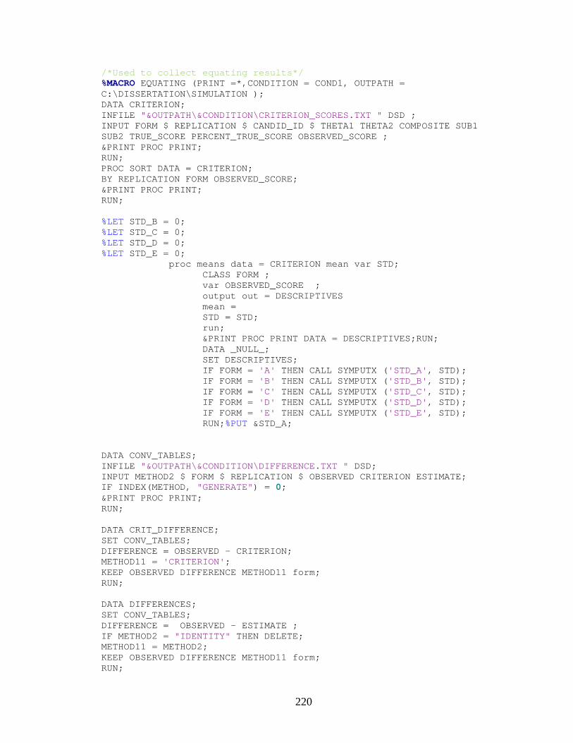
220

/*Used to collect equating results*/ %MACRO EQUATING (PRINT =*,CONDITION = COND1, OUTPATH = C:\DISSERTATION\SIMULATION ); DATA CRITERION; INFILE "&OUTPATH\&CONDITION\CRITERION_SCORES.TXT " DSD ; INPUT FORM $ REPLICATION $ CANDID_ID $ THETA1 THETA2 COMPOSITE SUB1 SUB2 TRUE_SCORE PERCENT_TRUE_SCORE OBSERVED_SCORE ; &PRINT PROC PRINT; RUN; PROC SORT DATA = CRITERION; BY REPLICATION FORM OBSERVED_SCORE; &PRINT PROC PRINT; RUN; %LET STD_B = 0; %LET STD_C = 0; %LET STD_D = 0; %LET STD_E = 0; proc means data = CRITERION mean var STD; CLASS FORM ; var OBSERVED_SCORE ; output out = DESCRIPTIVES mean = STD = STD; run; &PRINT PROC PRINT DATA = DESCRIPTIVES;RUN; DATA _NULL_; SET DESCRIPTIVES; IF FORM = 'A' THEN CALL SYMPUTX ('STD_A', STD); IF FORM = 'B' THEN CALL SYMPUTX ('STD_B', STD); IF FORM = 'C' THEN CALL SYMPUTX ('STD_C', STD); IF FORM = 'D' THEN CALL SYMPUTX ('STD_D', STD); IF FORM = 'E' THEN CALL SYMPUTX ('STD_E', STD); RUN;%PUT &STD_A; DATA CONV_TABLES; INFILE "&OUTPATH\&CONDITION\DIFFERENCE.TXT " DSD; INPUT METHOD2 $ FORM $ REPLICATION $ OBSERVED CRITERION ESTIMATE; IF INDEX(METHOD, "GENERATE") = 0; &PRINT PROC PRINT; RUN; DATA CRIT_DIFFERENCE; SET CONV_TABLES; DIFFERENCE = OBSERVED - CRITERION; METHOD11 = 'CRITERION'; KEEP OBSERVED DIFFERENCE METHOD11 form; RUN; DATA DIFFERENCES; SET CONV_TABLES; DIFFERENCE = OBSERVED - ESTIMATE ; IF METHOD2 = "IDENTITY" THEN DELETE; METHOD11 = METHOD2; KEEP OBSERVED DIFFERENCE METHOD11 form; RUN;

221

DATA DIFFERENCES; SET DIFFERENCES CRIT_DIFFERENCE; IF INDEX(METHOD11,'STOCK')>0 THEN METHOD1 = "4. SCSL "; IF INDEX(METHOD11,'LINEAR')>0 THEN METHOD1 = "2. LLTS "; IF INDEX(METHOD11,'FPC')>0 THEN METHOD1 = "3. FPC "; IF INDEX(METHOD11,'CRITERIO')>0 THEN METHOD1 = "1. CRITERION "; RUN; PROC MEANS DATA = DIFFERENCES NOPRINT; CLASS FORM METHOD1 OBSERVED; VAR DIFFERENCE; OUTPUT OUT = DIFF MEAN=; RUN; DATA DIFF; SET DIFF; IF _TYPE_ = 7; RUN; DATA DB DC DD DE; SET DIFF; IF FORM = "B" THEN OUTPUT DB; IF FORM = "C" THEN OUTPUT DC; IF FORM = "D" THEN OUTPUT DD; IF FORM = "E" THEN OUTPUT DE; RUN; &PRINT PROC PRINT DATA = DB;RUN; PROC SORT DATA = DB; BY FORM OBSERVED; RUN; PROC TRANSPOSE DATA = DB OUT = T_DB; ID METHOD1; VAR DIFFERENCE; BY FORM OBSERVED; RUN; PROC SORT DATA = DC; BY FORM OBSERVED; RUN; PROC TRANSPOSE DATA = DC OUT = T_DC; ID METHOD1; VAR DIFFERENCE; BY FORM OBSERVED; RUN; PROC SORT DATA = DD; BY FORM OBSERVED; RUN; PROC TRANSPOSE DATA = DD OUT = T_DD; ID METHOD1; VAR DIFFERENCE; BY FORM OBSERVED;

222

RUN; PROC SORT DATA = DE; BY FORM OBSERVED; RUN; PROC TRANSPOSE DATA = DE OUT = T_DE; ID METHOD1; VAR DIFFERENCE; BY FORM OBSERVED; RUN; /*ADD THE IDENTITY EQUATING*/ DATA IDENTITY; SET CONV_TABLES; IF METHOD2 = 'FPC'; IF REPLICATION = "REP1"; METHOD2 = "IDENTITY"; ESTIMATE = OBSERVED; &PRINT PROC PRINT;RUN; DATA CONV_TABLES; SET CONV_TABLES IDENTITY; RUN; DATA COND1_RESULTS; SET CONV_TABLES; BIAS = ESTIMATE- CRITERION; SQ_ERROR = (ESTIMATE- CRITERION)**2; &PRINT PROC PRINT; RUN; proc means data = COND1_RESULTS mean var ; CLASS FORM METHOD2 OBSERVED; var ESTIMATE BIAS SQ_ERROR ; output out = sqbias mean = STD = STD_ESTIMATE STD_BIAS STD_SQ_ERROR ; run; data sqbias2; set sqbias; LENGTH METHOD $12.; METHOD = METHOD2; if _type_ = 7; RMSE = SQRT(SQ_ERROR); ST_ERROR = SQRT(RMSE**2 - BIAS**2 ); DROP METHOD2; *KEEP _FREQ_ METHOD ESTIMATE BIAS RMSE ST_ERROR FORM _type_ ST_ERR_CRIT; proc sort; by FORM OBSERVED ; &PRINT PROC PRINT; run; &PRINT PROC PRINT DATA = SQBIAS2;RUN; DATA ST_ERR_CRIT; DO OBSERVED =0 TO 60 BY 1;

223

FORM = "B"; OUTPUT; END; DO OBSERVED =0 TO 60 BY 1; FORM = "C"; OUTPUT; END; DO OBSERVED =0 TO 60 BY 1; FORM = "D"; OUTPUT; END; DO OBSERVED =0 TO 60 BY 1; FORM = "E"; OUTPUT; END; RUN; DATA ST_ERR_CRIT; SET ST_ERR_CRIT; METHOD = "CRITERION"; IF FORM = 'B' THEN ST_ERROR = (.10* &STD_B); IF FORM = 'C' THEN ST_ERROR = (.10* &STD_C); IF FORM = 'D' THEN ST_ERROR = (.10* &STD_D); IF FORM = 'E' THEN ST_ERROR = (.10* &STD_E); &PRINT PROC PRINT;RUN; DATA SQBIAS2; SET SQBIAS2 ST_ERR_CRIT; &PRINT PROC PRINT; RUN; PROC SORT DATA = SQBIAS2; BY FORM; RUN; DATA SQBIAS3; SET SQBIAS2; IF METHOD = "IDENTITY" THEN DELETE; RUN; DATA B C D E; SET SQBIAS3; IF INDEX(METHOD,'STOCK')>0 THEN METHOD = "4. SCSL "; IF INDEX(METHOD,'LINEAR')>0 THEN METHOD = "2. LLTS "; IF INDEX(METHOD,'FPC')>0 THEN METHOD = "3. FPC "; IF INDEX(METHOD,'CRITERION')>0 THEN METHOD = "1. CRITERION "; IF FORM = "B" THEN OUTPUT B; IF FORM = "C" THEN OUTPUT C; IF FORM = "D" THEN OUTPUT D; IF FORM = "E" THEN OUTPUT E; RUN; &PRINT PROC PRINT DATA = B;RUN; /*NOW SYSTEMATIC ERROR*/ DATA SB SC SD SE;

224

SET SQBIAS2; IF INDEX(METHOD,"CRITER") = 0; IF INDEX(METHOD,'STOCK')>0 THEN METHOD = "4. SCSL"; IF INDEX(METHOD,'LINEAR')>0 THEN METHOD = "2. LLTS"; IF INDEX(METHOD,'FPC')>0 THEN METHOD = "3. FPC "; IF INDEX(METHOD,'IDENTITY')>0 THEN METHOD = "1. IDENTITY"; IF FORM = "B" THEN OUTPUT SB; IF FORM = "C" THEN OUTPUT SC; IF FORM = "D" THEN OUTPUT SD; IF FORM = "E" THEN OUTPUT SE; RUN; &PRINT PROC PRINT DATA = SB;RUN; PROC SORT DATA = SB; BY FORM OBSERVED; RUN; PROC TRANSPOSE DATA = SB OUT = T_SB; ID METHOD; VAR BIAS ST_ERROR; BY FORM OBSERVED; RUN; DATA T_BIAS_B ; SET T_SB; IF _NAME_ = 'BIAS' THEN OUTPUT T_BIAS_B; RUN; PROC SORT DATA = B; BY FORM OBSERVED; RUN; PROC TRANSPOSE DATA = B OUT = T_B; ID METHOD; VAR BIAS ST_ERROR; BY FORM OBSERVED; RUN; DATA T_RAND_B; SET T_B; IF _NAME_ = 'ST_ERROR' THEN OUTPUT T_RAND_B; RUN; /*C*/ PROC SORT DATA = SC; BY FORM OBSERVED; RUN; PROC TRANSPOSE DATA = SC OUT = T_SC; ID METHOD; VAR BIAS ST_ERROR; BY FORM OBSERVED; RUN; DATA T_BIAS_C ;

225

SET T_SC; IF _NAME_ = 'BIAS' THEN OUTPUT T_BIAS_C; RUN; PROC SORT DATA = C; BY FORM OBSERVED; RUN; PROC TRANSPOSE DATA = C OUT = T_C; ID METHOD; VAR BIAS ST_ERROR; BY FORM OBSERVED; RUN; DATA T_RAND_C; SET T_C; IF _NAME_ = 'ST_ERROR' THEN OUTPUT T_RAND_C; RUN; /*D*/ PROC SORT DATA = SD; BY FORM OBSERVED; RUN; PROC TRANSPOSE DATA = SD OUT = T_SD; ID METHOD; VAR BIAS ST_ERROR; BY FORM OBSERVED; RUN; DATA T_BIAS_D ; SET T_SD; IF _NAME_ = 'BIAS' THEN OUTPUT T_BIAS_D; RUN; PROC SORT DATA = D; BY FORM OBSERVED; RUN; PROC TRANSPOSE DATA = D OUT = T_D; ID METHOD; VAR BIAS ST_ERROR; BY FORM OBSERVED; RUN; DATA T_RAND_D; SET T_D; IF _NAME_ = 'ST_ERROR' THEN OUTPUT T_RAND_D; RUN; /*E*/ PROC SORT DATA = SE; BY FORM OBSERVED; RUN; PROC TRANSPOSE DATA = SE OUT = T_SE; ID METHOD; VAR BIAS ST_ERROR; BY FORM OBSERVED; RUN;

226

DATA T_BIAS_E ; SET T_SE; IF _NAME_ = 'BIAS' THEN OUTPUT T_BIAS_E; RUN; PROC SORT DATA = E; BY FORM OBSERVED; RUN; PROC TRANSPOSE DATA = E OUT = T_E; ID METHOD; VAR BIAS ST_ERROR; BY FORM OBSERVED; RUN; DATA T_RAND_E; SET T_E; IF _NAME_ = 'ST_ERROR' THEN OUTPUT T_RAND_E; RUN; proc print data = t_bias_e;run; %MEND; %macro delcat(catname); %if %sysfunc(cexist(&catname)) %then %do; proc greplay nofs igout=&catname; delete _all_; run; %end; quit; %mend delcat;

227

%MACRO PLOT (PRINT =*,FORM2 =B, FTEXT = SWISS, LIGHTTEXT = black, NOTE=, OUTPATH = C:\DISSERTATION\SIMULATION, CONDITION =COND1,DATASET =BOTH, LINE_NAME=THETA, NAME = PLOT1, YAXIS = COUNT, XAXIS=VALUE, MIN_X= -4, MAX_X = 4, BY =1, MIN_Y=0, MAX_Y = 1, BY_Y = .25, TITLE = THETAS, SUB_TITLE= , Y_LABEL=COUNT, X_LABEL =THETA, START_LEGEND = 25, START_SYMBOL= 30, START_Y = 75, COLOR1 = GREEN, COLOR2 =BLUE, COLOR3 = ORANGE, COLOR4 = BLACK, COLOR5 = PURPLE, COLOR6 =RED, JOIN_POINTS=J, VREF=0, POSITION_=TOP LEFT INSIDE, ACROSS = 1, DOWN =4, CAPTION=, SPECIAL=); OPTIONS NOXWAIT ; Data _null_; call system ("mkdir &OUTPATH\&CONDITION\RESULTS\&FORM2"); RUN; data data3; set &dataset; length html $400; html= 'title='||quote(trim(left(round(percent,.01 )))||'% of examiness earned a score of '|| trim(left(&XAXIS))|| ' on THETA'||trim(left(&LINE_NAME))||'.' ) ||' '|| 'href="'||"/files/HTML_FILES/SC.html"||'"'; &PRINT PROC PRINT; run; /*make LEGEND for plot*/ proc freq data = &dataset NOPRINT; table &LINE_NAME/out= LINE_NAME; run; DATA LINE_NAME2; SET LINE_NAME; order =0; order2 = 0; b = 0; drop count percent; proc sort; by &LINE_NAME ; &PRINT PROC PRINT; RUN; DATA _NULL_; SET LINE_NAME2; BLANK = " "; CALL SYMPUTX ('FIRST',BLANK ); CALL SYMPUTX ('SEC',BLANK); CALL SYMPUTX ('THIRD',BLANK); CALL SYMPUTX ('FOURTH',BLANK ); CALL SYMPUTX ('FIFTH',BLANK ); CALL SYMPUTX ('SIXTH',BLANK); RUN; DATA _NULL_;

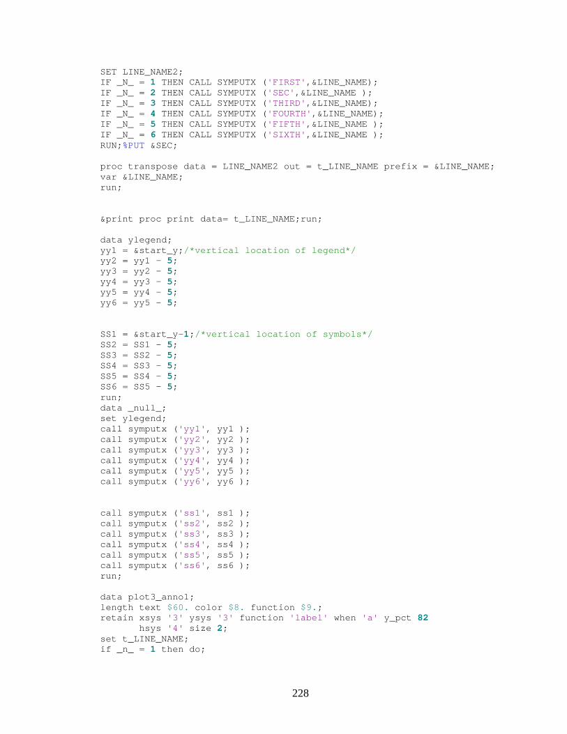
228

SET LINE_NAME2; IF _N_ = 1 THEN CALL SYMPUTX ('FIRST',&LINE_NAME); IF _N_ = 2 THEN CALL SYMPUTX ('SEC',&LINE_NAME ); IF _N_ = 3 THEN CALL SYMPUTX ('THIRD',&LINE_NAME); IF _N_ = 4 THEN CALL SYMPUTX ('FOURTH',&LINE_NAME); IF _N_ = 5 THEN CALL SYMPUTX ('FIFTH',&LINE_NAME ); IF _N_ = 6 THEN CALL SYMPUTX ('SIXTH',&LINE_NAME ); RUN;%PUT &SEC; proc transpose data = LINE_NAME2 out = t_LINE_NAME prefix = &LINE_NAME; var &LINE_NAME; run; &print proc print data= t_LINE_NAME;run; data ylegend; yy1 = &start_y;/*vertical location of legend*/ yy2 = yy1 - 5; yy3 = yy2 - 5; yy4 = yy3 - 5; yy5 = yy4 - 5; yy6 = yy5 - 5; SS1 = &start_y-1;/*vertical location of symbols*/ SS2 = SS1 - 5; SS3 = SS2 - 5; SS4 = SS3 - 5; SS5 = SS4 - 5; SS6 = SS5 - 5; run; data _null_; set ylegend; call symputx ('yy1', yy1 ); call symputx ('yy2', yy2 ); call symputx ('yy3', yy3 ); call symputx ('yy4', yy4 ); call symputx ('yy5', yy5 ); call symputx ('yy6', yy6 ); call symputx ('ss1', ss1 ); call symputx ('ss2', ss2 ); call symputx ('ss3', ss3 ); call symputx ('ss4', ss4 ); call symputx ('ss5', ss5 ); call symputx ('ss6', ss6 ); run; data plot3_anno1; length text $60. color $8. function $9.; retain xsys '3' ysys '3' function 'label' when 'a' y_pct 82 hsys '4' size 2; set t_LINE_NAME; if _n_ = 1 then do;

229

x=&START_LEGEND; y=&yy1; text="&FIRST "; color="&COLOR1" ;style="&ftext"; output; x=&START_LEGEND; y=&yy2; text="&SEC "; color="&COLOR2" ; output; x=&START_LEGEND; y=&yy3; text="&THIRD "; color="&COLOR3" ; output; x=&START_LEGEND; y=&yy4; text="&FOURTH "; color="&COLOR4" ;style="&ftext"; output; /* x=&START_LEGEND; y=&yy5; text="&FIFTH "; color="&COLOR5" ; output; x=&START_LEGEND; y=&yy6; text="&SIXTH "; color="&COLOR6" ; output;*/ x=55; y=86; text="&SUB_TITLE "; color="&lighttext" ; size = 3.00; output; when='a'; style="&ftext"; color="&lighttext"; hsys='3'; size=6; function='label'; xsys='1'; x=50; ysys='3'; y=15; position='5'; text="&X_LABEL"; output; when='a'; style="&ftext"; color="&lighttext"; hsys='3'; size=6; function='label'; xsys='1'; x=50; ysys='3'; y=8; position='5'; text="&CAPTION"; output; FUNCTION = 'SYMBOL'; style = " "; TEXT = "DOT "; color="&COLOR1" ; x=&START_SYMBOL; y=&ss1; size = 5.00; output; FUNCTION = 'SYMBOL';TEXT = "TRIANGLE "; color="&COLOR2" ; x=&START_SYMBOL; y=&ss2; size = 5.00; output; FUNCTION = 'SYMBOL'; TEXT = "SQUARE"; color="&COLOR3" ; x=&START_SYMBOL; y=&ss3; size = 5.00; output; FUNCTION = 'SYMBOL'; TEXT = "CIRCLE "; color="&COLOR4" ; x=&START_SYMBOL; y=&ss4; size = 5.00; output; FUNCTION = 'SYMBOL'; style = " "; TEXT = "DOT "; color="&COLOR1" ; x=&START_SYMBOL +4; y=&ss1; size = 5.00; output; FUNCTION = 'SYMBOL';TEXT = "TRIANGLE "; color="&COLOR2" ; x=&START_SYMBOL +4; y=&ss2; size = 5.00; output; FUNCTION = 'SYMBOL'; TEXT = "SQUARE"; color="&COLOR3" ; x=&START_SYMBOL +4; y=&ss3; size = 5.00; output; FUNCTION = 'SYMBOL'; TEXT = "CIRCLE "; color="&COLOR4" ; x=&START_SYMBOL +4; y=&ss4; size = 5.00; output; FUNCTION = 'SYMBOL'; style = " "; TEXT = "DOT "; color="&COLOR1" ; x=&START_SYMBOL +8; y=&ss1; size = 5.00; output; FUNCTION = 'SYMBOL';TEXT = "TRIANGLE "; color="&COLOR2" ; x=&START_SYMBOL +8; y=&ss2; size = 5.00; output; FUNCTION = 'SYMBOL'; TEXT = "SQUARE"; color="&COLOR3" ; x=&START_SYMBOL +8; y=&ss3; size = 5.00; output; FUNCTION = 'SYMBOL'; TEXT = "CIRCLE "; color="&COLOR4" ; x=&START_SYMBOL +8; y=&ss4; size = 5.00; output;

230

function='move'; x=&START_SYMBOL -3; y=&ss1 ; color="&COLOR1"; SIZE = 2; output; function='draw'; X=&START_SYMBOL+11; output; function='move'; x=&START_SYMBOL -3; y=&ss2 ; color="&COLOR2"; SIZE = 2; output; function='draw'; X=&START_SYMBOL+11; output; function='move'; x=&START_SYMBOL -3; y=&ss3; color="&COLOR3"; SIZE = 2; output; function='draw'; X=&START_SYMBOL+11; output; function='move'; x=&START_SYMBOL -3; y=&ss4 ; color="&COLOR4"; SIZE = 2; output; function='draw'; X=&START_SYMBOL+11; output; end; &print proc print; run; /*end of LEGEND*/ FILENAME GRAPHOUT "&OUTPATH\&CONDITION\RESULTS\&FORM2"; GOPTIONS RESET=ALL DEVICE = GIF GSFNAME=GRAPHOUT ; options mlogic symbolgen; goptions xpixels=300 ypixels=200; goptions gunit=pct htitle=8 htext=5 ftitle=&ftext ftext=&ftext ctext=&lighttext; %LET MAJORCOLOR =BLUE ;*cx50A6C2; %LET FTEXT = 'SWISS'; axis1 color=&lighttext minor=none label=(a = 90 font = 'swiss' "&y_label" ) order = (&min_Y to &max_Y by &by_Y )offset=(0,0); axis2 color=&lighttext minor=none label = none major=none order = (&min_X to &max_X by &by ) offset=(2,2) style=0;/**/ %IF &TITLE = _ %THEN %DO; title1 j=l c=WHITE "&TITLE"; %END; footnote1 h=10 " "; proc sort data = data3; by &LINE_NAME; &PRINT PROC PRINT; run; data line_name; set line_name; drop count percent; run; proc sort data = LINE_NAME; by &LINE_NAME;run; data data34; merge data3 (in=u) LINE_NAME; by &LINE_NAME; if u;

231

run; legend1 LABEL = NONE value = ("&FIRST " "&SEC" "&THIRD" "&FOURTH " "&FIFTH ") ACROSS = &ACROSS DOWN = &DOWN POSITION = (&position_) MODE =PROTECT CFRAME = WHITE OFFSET = (1 PCT); symbol1 i=&JOIN_POINTS v=dot c=&COLOR1 w=2 h=4 ; symbol2 i=&JOIN_POINTS v=TRIANGLE c=&COLOR2 w=2 h=4 ; symbol3 i=&JOIN_POINTS v=SQUARE c=&COLOR3 w=2 h=4 ; symbol4 i=&JOIN_POINTS v=CIRCLE c=&COLOR4 w=2 h=4 ; TITLE2 ' '; %IF &SPECIAL = %THEN %DO; proc gplot data=data34 anno=plot3_anno1;/* */ plot &YAXIS*&XAXIS=&LINE_NAME / haxis = axis2 vaxis=axis1 vref=&VREF noframe name="&NAME" NOLEGEND HTML = HTML; run; quit; %END; %IF &SPECIAL = Y %THEN %DO; symbol1 i=&JOIN_POINTS v=NONE c=&COLOR1 w=4 h=4 ; symbol2 i=&JOIN_POINTS v=NONE c=&COLOR2 w=4 h=4 ; symbol3 i=&JOIN_POINTS v=NONE c=&COLOR3 w=4 h=4 ; symbol4 i=&JOIN_POINTS v=NONE c=&COLOR4 w=4 h=4 ; symbol5 i=NONE v=DOT c=&COLOR1 w=4 h=5 ; symbol6 i=NONE v=TRIANGLE c=&COLOR2 w=4 h=5 ; symbol7 i=NONE v=SQUARE c=&COLOR3 w=4 h=5 ; symbol8 i=NONE v=CIRCLE c=&COLOR4 w=4 h=5 ; %IF %UPCASE(&Y_LABEL) = BIAS %THEN %DO; %LET D_SET = T_BIAS_&FORM2; %LET CRIT=IDENTITY; %END; %IF %UPCASE(&Y_LABEL) NE BIAS %THEN %DO; %LET D_SET = T_RAND_&FORM2; %LET CRIT=CRITERION; %END; %IF %UPCASE(&Y_LABEL) EQ DIFFERENCE %THEN %DO; %LET D_SET = T_D&FORM2; %LET CRIT=CRITERION; %END; DATA &D_SET;

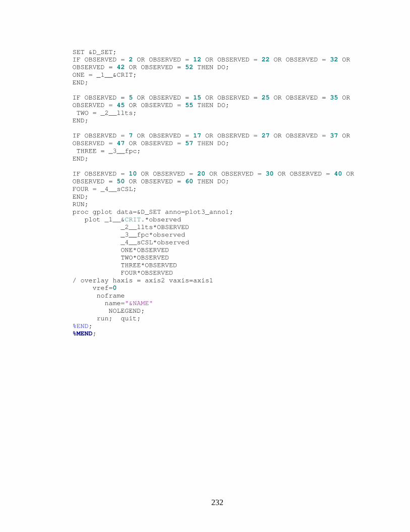
232

SET &D_SET; IF OBSERVED = 2 OR OBSERVED = 12 OR OBSERVED = 22 OR OBSERVED = 32 OR OBSERVED = 42 OR OBSERVED = 52 THEN DO; ONE = _1__&CRIT; END; IF OBSERVED = 5 OR OBSERVED = 15 OR OBSERVED = 25 OR OBSERVED = 35 OR OBSERVED = 45 OR OBSERVED = 55 THEN DO; TWO = _2__llts; END; IF OBSERVED = 7 OR OBSERVED = 17 OR OBSERVED = 27 OR OBSERVED = 37 OR OBSERVED = 47 OR OBSERVED = 57 THEN DO; THREE = _3__fpc; END; IF OBSERVED = 10 OR OBSERVED = 20 OR OBSERVED = 30 OR OBSERVED = 40 OR OBSERVED = 50 OR OBSERVED = 60 THEN DO; FOUR = _4__sCSL; END; RUN; proc gplot data=&D_SET anno=plot3_anno1; plot _1__&CRIT.*observed _2__llts*OBSERVED _3__fpc*observed _4__sCSL*observed ONE*OBSERVED TWO*OBSERVED THREE*OBSERVED FOUR*OBSERVED / overlay haxis = axis2 vaxis=axis1 vref=0 noframe name="&NAME" NOLEGEND; run; quit; %END; %MEND;

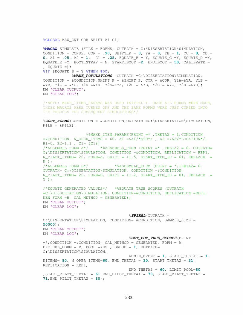
233

%GLOBAL MAX_CNT COR SHIFT A1 C1; %MACRO SIMULATE (FILE = FORMS, OUTPATH = C:\DISSERTATION\SIMULATION, CONDITION = COND2, COR = .90, SHIFT_P = 0, YA = 0, YB = 1, YC = 0, YD = 0, A1 = .05, A2 = 1, C1 = .25, EQUATE_B = Y, EQUATE_C =Y, EQUATE_D =Y, EQUATE_E =Y, BOOT_STRAP = N, START_BOOT =2, END_BOOT = 50, CALIBRATE = , EQUATE =); %IF &EQUATE_B = Y %THEN %DO; %MAKE_POPULATIONS (OUTPATH =C:\DISSERTATION\SIMULATION, CONDITION = &CONDITION,SHIFT_P = &SHIFT_P, COR = &COR, Y1A=&YA, Y1B = &YB, Y1C = &YC, Y1D =&YD, Y2A=&YA, Y2B = &YB, Y2C = &YC, Y2D =&YD); DM "CLEAR OUTPUT"; DM "CLEAR LOG"; /*NOTE: MAKE_ITEMS_PARAMS WAS USED INITIALLY. ONCE ALL FORMS WERE MADE, THESE MACROS WERE TURNED OFF AND THE SAME FORMS WERE JUST COPIED INTO THE FOLDERS FOR SUBSEQUENT SIMULATIONS*/ %COPY_FORMS(CONDITION = &CONDITION,OUTPATH =C:\DISSERTATION\SIMULATION, FILE = &FILE); *%MAKE_ITEM_PARAMS(PRINT =* ,THETA2 = 1,CONDITION =&CONDITION, N_OPER_ITEMS = 60, A1 =&A1/*STD*/ , A2 =&A2/*LOCATION*/, B1=0, B2=1.1 , C1= &C1); /*ASSEMBLE FORM A*/ *%ASSEMBLE_FORM (PRINT =* ,THETA2 = 0, OUTPATH= C:\DISSERTATION\SIMULATION, CONDITION =&CONDITION, REPLICATION = REP1, N_PILOT_ITEMS= 20, FORM=A, SHIFT = +1.5, START_ITEM_ID = 61, REPLACE = N ); /*ASSEMBLE FORM B*/ *%ASSEMBLE_FORM (PRINT = *,THETA2= 0, OUTPATH= C:\DISSERTATION\SIMULATION, CONDITION =&CONDITION, N_PILOT_ITEMS= 20, FORM=B, SHIFT = +1.2, START_ITEM_ID = 81, REPLACE = Y ); /*EQUATE GENERATED VALUES*/ *%EQUATE_TRUE_SCORES (OUTPATH =C:\DISSERTATION\SIMULATION, CONDITION=&CONDITION, REPLICATION =REP1, NEW_FORM =B, CAL_METHOD = GENERATED); DM "CLEAR OUTPUT"; DM "CLEAR LOG"; %SPIRAL(OUTPATH = C:\DISSERTATION\SIMULATION, CONDITION= &CONDITION, SAMPLE_SIZE = 50000); DM "CLEAR OUTPUT"; DM "CLEAR LOG"; %GET_POP_TRUE_SCORES(PRINT =*,CONDITION =&CONDITION, CAL_METHOD = GENERATED, FORM = A, EXCLUDE_FORM = B, POOL =YES , GROUP = 1, OUTPATH= C:\DISSERTATION\SIMULATION, ADMIN_EVENT = 1, START_THETA1 = 1, NITEMS= 80, N_OPER_ITEMS=60, END_THETA1 = 30, START_THETA2 = 31, REPLICATION = REP1, END_THETA2 = 60, LIMIT_POOL=80 ,START_PILOT_THETA1 = 61,END_PILOT_THETA1 = 70, START_PILOT_THETA2 = 71,END_PILOT_THETA2 = 80);

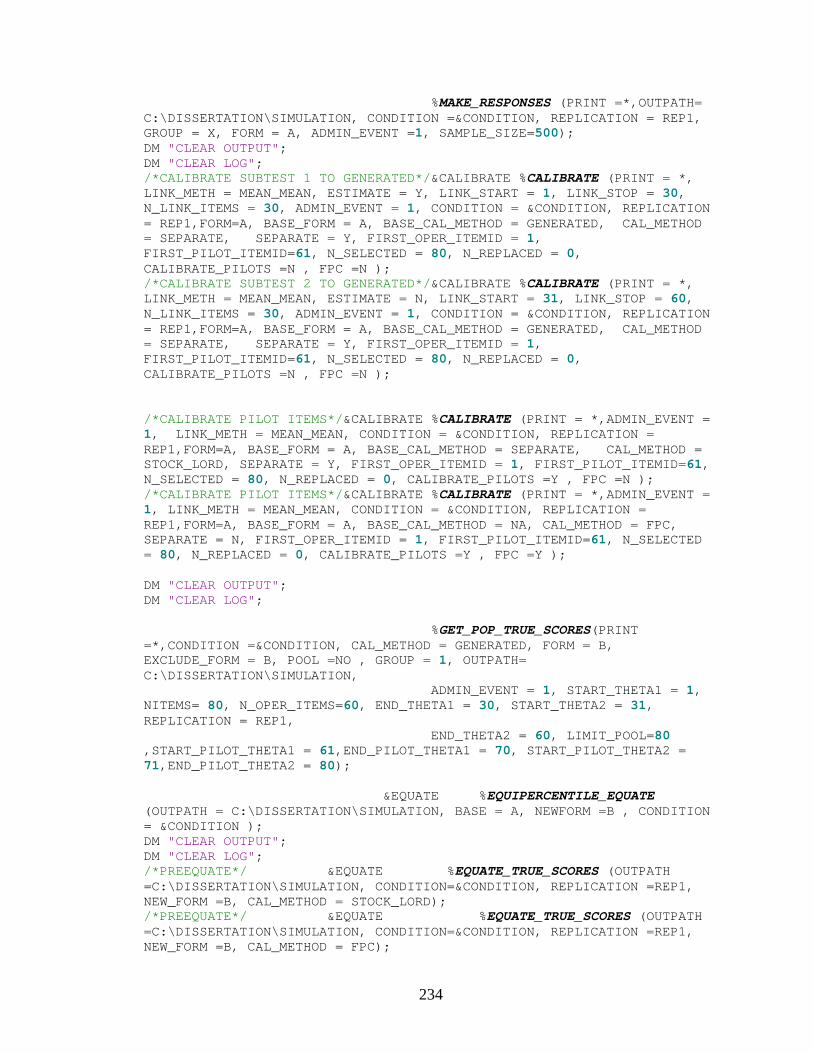
234

%MAKE_RESPONSES (PRINT =*,OUTPATH= C:\DISSERTATION\SIMULATION, CONDITION =&CONDITION, REPLICATION = REP1, GROUP = X, FORM = A, ADMIN_EVENT =1, SAMPLE_SIZE=500); DM "CLEAR OUTPUT"; DM "CLEAR LOG"; /*CALIBRATE SUBTEST 1 TO GENERATED*/&CALIBRATE %CALIBRATE (PRINT = *, LINK_METH = MEAN_MEAN, ESTIMATE = Y, LINK_START = 1, LINK_STOP = 30, N_LINK_ITEMS = 30, ADMIN_EVENT = 1, CONDITION = &CONDITION, REPLICATION = REP1,FORM=A, BASE_FORM = A, BASE_CAL_METHOD = GENERATED, CAL_METHOD = SEPARATE, SEPARATE = Y, FIRST_OPER_ITEMID = 1, FIRST_PILOT_ITEMID=61, N_SELECTED = 80, N_REPLACED = 0, CALIBRATE_PILOTS =N , FPC =N ); /*CALIBRATE SUBTEST 2 TO GENERATED*/&CALIBRATE %CALIBRATE (PRINT = *, LINK_METH = MEAN_MEAN, ESTIMATE = N, LINK_START = 31, LINK_STOP = 60, N_LINK_ITEMS = 30, ADMIN_EVENT = 1, CONDITION = &CONDITION, REPLICATION = REP1,FORM=A, BASE_FORM = A, BASE_CAL_METHOD = GENERATED, CAL_METHOD = SEPARATE, SEPARATE = Y, FIRST_OPER_ITEMID = 1, FIRST_PILOT_ITEMID=61, N_SELECTED = 80, N_REPLACED = 0, CALIBRATE_PILOTS =N , FPC =N ); /*CALIBRATE PILOT ITEMS*/&CALIBRATE %CALIBRATE (PRINT = *,ADMIN_EVENT = 1, LINK_METH = MEAN_MEAN, CONDITION = &CONDITION, REPLICATION = REP1,FORM=A, BASE_FORM = A, BASE_CAL_METHOD = SEPARATE, CAL_METHOD = STOCK_LORD, SEPARATE = Y, FIRST_OPER_ITEMID = 1, FIRST_PILOT_ITEMID=61, N_SELECTED = 80, N_REPLACED = 0, CALIBRATE_PILOTS =Y , FPC =N ); /*CALIBRATE PILOT ITEMS*/&CALIBRATE %CALIBRATE (PRINT = *,ADMIN_EVENT = 1, LINK_METH = MEAN_MEAN, CONDITION = &CONDITION, REPLICATION = REP1,FORM=A, BASE_FORM = A, BASE_CAL_METHOD = NA, CAL_METHOD = FPC, SEPARATE = N, FIRST_OPER_ITEMID = 1, FIRST_PILOT_ITEMID=61, N_SELECTED = 80, N_REPLACED = 0, CALIBRATE_PILOTS =Y , FPC =Y ); DM "CLEAR OUTPUT"; DM "CLEAR LOG"; %GET_POP_TRUE_SCORES(PRINT =*,CONDITION =&CONDITION, CAL_METHOD = GENERATED, FORM = B, EXCLUDE_FORM = B, POOL =NO , GROUP = 1, OUTPATH= C:\DISSERTATION\SIMULATION, ADMIN_EVENT = 1, START_THETA1 = 1, NITEMS= 80, N_OPER_ITEMS=60, END_THETA1 = 30, START_THETA2 = 31, REPLICATION = REP1, END_THETA2 = 60, LIMIT_POOL=80 ,START_PILOT_THETA1 = 61,END_PILOT_THETA1 = 70, START_PILOT_THETA2 = 71,END_PILOT_THETA2 = 80); &EQUATE %EQUIPERCENTILE_EQUATE (OUTPATH = C:\DISSERTATION\SIMULATION, BASE = A, NEWFORM =B , CONDITION = &CONDITION ); DM "CLEAR OUTPUT"; DM "CLEAR LOG"; /*PREEQUATE*/ &EQUATE %EQUATE_TRUE_SCORES (OUTPATH =C:\DISSERTATION\SIMULATION, CONDITION=&CONDITION, REPLICATION =REP1, NEW_FORM =B, CAL_METHOD = STOCK_LORD); /*PREEQUATE*/ &EQUATE %EQUATE_TRUE_SCORES (OUTPATH =C:\DISSERTATION\SIMULATION, CONDITION=&CONDITION, REPLICATION =REP1, NEW_FORM =B, CAL_METHOD = FPC);

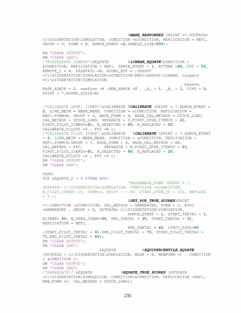
235

%MAKE_RESPONSES (PRINT =*,OUTPATH= C:\DISSERTATION\SIMULATION, CONDITION =&CONDITION, REPLICATION = REP1, GROUP = Y, FORM = B, ADMIN_EVENT =2,SAMPLE_SIZE=500); DM "CLEAR OUTPUT"; DM "CLEAR LOG"; /*POSTEQUATE LINEAR*/&EQUATE %LINEAR_EQUATE(CONDITION = &CONDITION, REPLICATION = REP1, ADMIN_EVENT = 1, NITEMS =60, CUT = 55, REMOVE_C = N, PASSFAIL =N, ROUND_BUF = ,ODSOUT =C:\DISSERTATION\SIMULATION\&CONDITION\REP1\ADMIN2\LINEAR, outpath =C:\DISSERTATION\SIMULATION, base=A, BASE_ADMIN = 1, newform =B ,NEW_ADMIN =2 , _A_ = 1, _B_ = 1, CIPE = N, PRINT = *,ROUND_SCALE=N) /*CALIBRATE OPER. ITEMS*/&CALIBRATE %CALIBRATE (PRINT = *,ADMIN_EVENT = 2, LINK_METH = MEAN_MEAN, CONDITION = &CONDITION, REPLICATION = REP1,FORM=B, GROUP = Y, BASE_FORM = A, BASE_CAL_METHOD = STOCK_LORD, CAL_METHOD = STOCK_LORD, SEPARATE = Y,FIRST_OPER_ITEMID = 21, FIRST_PILOT_ITEMID=81, N_SELECTED = 80, N_REPLACED = 20, CALIBRATE_PILOTS =Y , FPC =N ); /*CALIBRATE PILOT ITEMS*/&CALIBRATE %CALIBRATE (PRINT = *,ADMIN_EVENT = 2, LINK_METH = MEAN_MEAN, CONDITION = &CONDITION, REPLICATION = REP1,FORM=B,GROUP = Y, BASE_FORM = A, BASE_CAL_METHOD = NA, CAL_METHOD = FPC, SEPARATE = N,FIRST_OPER_ITEMID = 21, FIRST_PILOT_ITEMID=81, N_SELECTED = 80, N_REPLACED = 20, CALIBRATE_PILOTS =Y , FPC =Y ); DM "CLEAR OUTPUT"; DM "CLEAR LOG"; %END; %IF &EQUATE_C = Y %THEN %DO; *%ASSEMBLE_FORM (PRINT = *, OUTPATH= C:\DISSERTATION\SIMULATION, CONDITION =&CONDITION, N_PILOT_ITEMS= 20, FORM=C, SHIFT = -.50, START_ITEM_ID = 101, REPLACE = Y ); %GET_POP_TRUE_SCORES(PRINT =*,CONDITION =&CONDITION, CAL_METHOD = GENERATED, FORM = C, POOL =GENERATED , GROUP = 1, OUTPATH= C:\DISSERTATION\SIMULATION, ADMIN_EVENT = 1, START_THETA1 = 1, NITEMS= 80, N_OPER_ITEMS=60, END_THETA1 = 30, START_THETA2 = 31, REPLICATION = REP1, END_THETA2 = 60, LIMIT_POOL=80 ,START_PILOT_THETA1 = 61,END_PILOT_THETA1 = 70, START_PILOT_THETA2 = 71,END_PILOT_THETA2 = 80); DM "CLEAR OUTPUT"; DM "CLEAR LOG"; &EQUATE %EQUIPERCENTILE_EQUATE (OUTPATH = C:\DISSERTATION\SIMULATION, BASE = A, NEWFORM =C , CONDITION = &CONDITION ); DM "CLEAR OUTPUT"; DM "CLEAR LOG"; /*PREEQUATE*/ &EQUATE %EQUATE_TRUE_SCORES (OUTPATH =C:\DISSERTATION\SIMULATION, CONDITION=&CONDITION, REPLICATION =REP1, NEW_FORM =C, CAL_METHOD = STOCK_LORD);

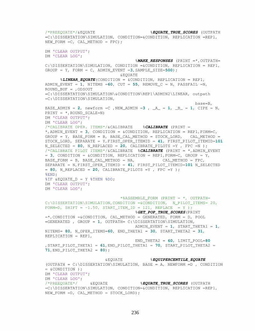
236

/*PREEQUATE*/&EQUATE %EQUATE_TRUE_SCORES (OUTPATH =C:\DISSERTATION\SIMULATION, CONDITION=&CONDITION, REPLICATION =REP1, NEW_FORM =C, CAL_METHOD = FPC); DM "CLEAR OUTPUT"; DM "CLEAR LOG"; %MAKE_RESPONSES (PRINT =*,OUTPATH= C:\DISSERTATION\SIMULATION, CONDITION =&CONDITION, REPLICATION = REP1, GROUP = Y, FORM = C, ADMIN_EVENT =3,SAMPLE_SIZE=500); &EQUATE %LINEAR_EQUATE(CONDITION = &CONDITION, REPLICATION = REP1, ADMIN_EVENT = 1, NITEMS =60, CUT = 55, REMOVE_C = N, PASSFAIL =N, ROUND_BUF = ,ODSOUT =C:\DISSERTATION\SIMULATION\&CONDITION\REP1\ADMIN2\LINEAR, outpath =C:\DISSERTATION\SIMULATION, base=B, BASE_ADMIN = 2, newform =C ,NEW_ADMIN =3 , _A_ = 1, _B_ = 1, CIPE = N, PRINT = *,ROUND_SCALE=N) DM "CLEAR OUTPUT"; DM "CLEAR LOG"; /*CALIBRATE OPER. ITEMS*/&CALIBRATE %CALIBRATE (PRINT = *,ADMIN_EVENT = 3, CONDITION = &CONDITION, REPLICATION = REP1,FORM=C, GROUP = Y, BASE_FORM = B, BASE_CAL_METHOD = STOCK_LORD, CAL_METHOD = STOCK_LORD, SEPARATE = Y,FIRST_OPER_ITEMID = 41, FIRST_PILOT_ITEMID=101 N_SELECTED = 80, N_REPLACED = 20, CALIBRATE_PILOTS =Y , FPC =N ); /*CALIBRATE PILOT ITEMS*/&CALIBRATE %CALIBRATE (PRINT = *,ADMIN_EVENT = 3, CONDITION = &CONDITION, REPLICATION = REP1,FORM=C, GROUP = Y, BASE_FORM = B, BASE_CAL_METHOD = NA, CAL_METHOD = FPC, SEPARATE = N,FIRST_OPER_ITEMID = 41, FIRST_PILOT_ITEMID=101 N_SELECTED = 80, N_REPLACED = 20, CALIBRATE_PILOTS =Y , FPC =Y ); %END; %IF &EQUATE_D = Y %THEN %DO; DM "CLEAR OUTPUT"; DM "CLEAR LOG"; *%ASSEMBLE_FORM (PRINT = *, OUTPATH= C:\DISSERTATION\SIMULATION,CONDITION =&CONDITION, N_PILOT_ITEMS= 20, FORM=D, SHIFT = -1.50, START_ITEM_ID = 121, REPLACE = Y ); %GET_POP_TRUE_SCORES(PRINT =*,CONDITION =&CONDITION, CAL_METHOD = GENERATED, FORM = D, POOL =GENERATED , GROUP = 1, OUTPATH= C:\DISSERTATION\SIMULATION, ADMIN_EVENT = 1, START_THETA1 = 1, NITEMS= 80, N_OPER_ITEMS=60, END_THETA1 = 30, START_THETA2 = 31, REPLICATION = REP1, END_THETA2 = 60, LIMIT_POOL=80 ,START_PILOT_THETA1 = 61,END_PILOT_THETA1 = 70, START_PILOT_THETA2 = 71,END_PILOT_THETA2 = 80); &EQUATE %EQUIPERCENTILE_EQUATE (OUTPATH = C:\DISSERTATION\SIMULATION, BASE = A, NEWFORM =D , CONDITION = &CONDITION ); DM "CLEAR OUTPUT"; DM "CLEAR LOG"; /*PREEQUATE*/ &EQUATE %EQUATE_TRUE_SCORES (OUTPATH =C:\DISSERTATION\SIMULATION, CONDITION=&CONDITION, REPLICATION =REP1, NEW_FORM =D, CAL_METHOD = STOCK_LORD);

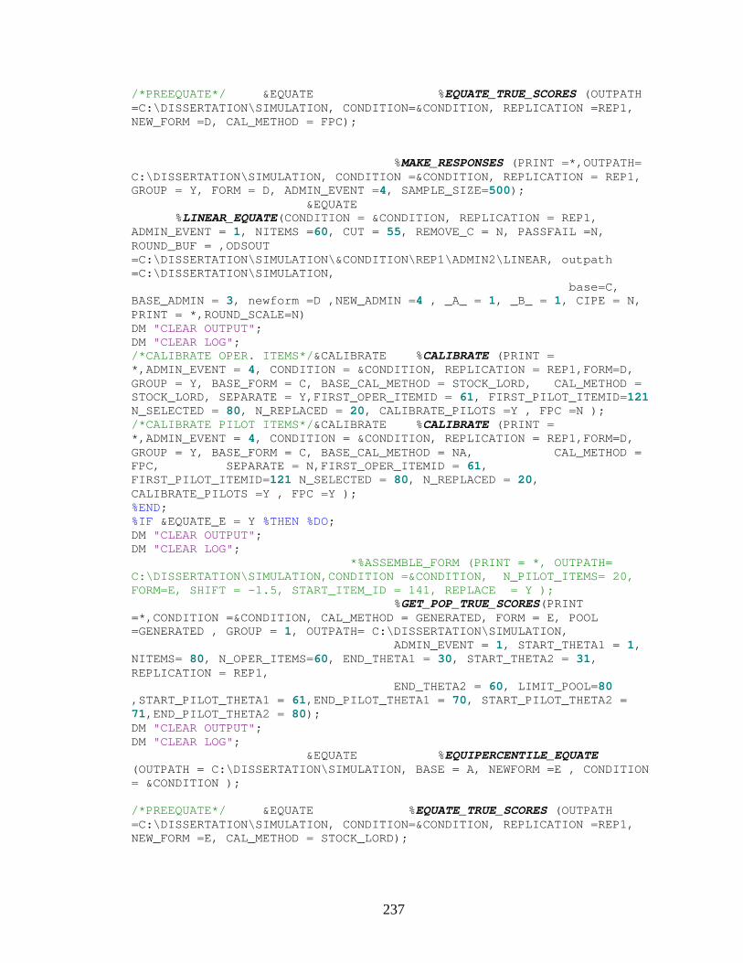
237

/*PREEQUATE*/ &EQUATE %EQUATE_TRUE_SCORES (OUTPATH =C:\DISSERTATION\SIMULATION, CONDITION=&CONDITION, REPLICATION =REP1, NEW_FORM =D, CAL_METHOD = FPC); %MAKE_RESPONSES (PRINT =*,OUTPATH= C:\DISSERTATION\SIMULATION, CONDITION =&CONDITION, REPLICATION = REP1, GROUP = Y, FORM = D, ADMIN_EVENT =4, SAMPLE_SIZE=500); &EQUATE %LINEAR_EQUATE(CONDITION = &CONDITION, REPLICATION = REP1, ADMIN_EVENT = 1, NITEMS =60, CUT = 55, REMOVE_C = N, PASSFAIL =N, ROUND_BUF = ,ODSOUT =C:\DISSERTATION\SIMULATION\&CONDITION\REP1\ADMIN2\LINEAR, outpath =C:\DISSERTATION\SIMULATION, base=C, BASE_ADMIN = 3, newform =D ,NEW_ADMIN =4 , _A_ = 1, _B_ = 1, CIPE = N, PRINT = *,ROUND_SCALE=N) DM "CLEAR OUTPUT"; DM "CLEAR LOG"; /*CALIBRATE OPER. ITEMS*/&CALIBRATE %CALIBRATE (PRINT = *,ADMIN_EVENT = 4, CONDITION = &CONDITION, REPLICATION = REP1,FORM=D, GROUP = Y, BASE_FORM = C, BASE_CAL_METHOD = STOCK_LORD, CAL_METHOD = STOCK_LORD, SEPARATE = Y,FIRST_OPER_ITEMID = 61, FIRST_PILOT_ITEMID=121 N_SELECTED = 80, N_REPLACED = 20, CALIBRATE_PILOTS =Y , FPC =N ); /*CALIBRATE PILOT ITEMS*/&CALIBRATE %CALIBRATE (PRINT = *,ADMIN_EVENT = 4, CONDITION = &CONDITION, REPLICATION = REP1,FORM=D, GROUP = Y, BASE_FORM = C, BASE_CAL_METHOD = NA, CAL_METHOD = FPC, SEPARATE = N,FIRST_OPER_ITEMID = 61, FIRST_PILOT_ITEMID=121 N_SELECTED = 80, N_REPLACED = 20, CALIBRATE_PILOTS =Y , FPC =Y ); %END; %IF &EQUATE_E = Y %THEN %DO; DM "CLEAR OUTPUT"; DM "CLEAR LOG"; *%ASSEMBLE_FORM (PRINT = *, OUTPATH= C:\DISSERTATION\SIMULATION,CONDITION =&CONDITION, N_PILOT_ITEMS= 20, FORM=E, SHIFT = -1.5, START_ITEM_ID = 141, REPLACE = Y ); %GET_POP_TRUE_SCORES(PRINT =*,CONDITION =&CONDITION, CAL_METHOD = GENERATED, FORM = E, POOL =GENERATED , GROUP = 1, OUTPATH= C:\DISSERTATION\SIMULATION, ADMIN_EVENT = 1, START_THETA1 = 1, NITEMS= 80, N_OPER_ITEMS=60, END_THETA1 = 30, START_THETA2 = 31, REPLICATION = REP1, END_THETA2 = 60, LIMIT_POOL=80 ,START_PILOT_THETA1 = 61,END_PILOT_THETA1 = 70, START_PILOT_THETA2 = 71,END_PILOT_THETA2 = 80); DM "CLEAR OUTPUT"; DM "CLEAR LOG"; &EQUATE %EQUIPERCENTILE_EQUATE (OUTPATH = C:\DISSERTATION\SIMULATION, BASE = A, NEWFORM =E , CONDITION = &CONDITION ); /*PREEQUATE*/ &EQUATE %EQUATE_TRUE_SCORES (OUTPATH =C:\DISSERTATION\SIMULATION, CONDITION=&CONDITION, REPLICATION =REP1, NEW_FORM =E, CAL_METHOD = STOCK_LORD);

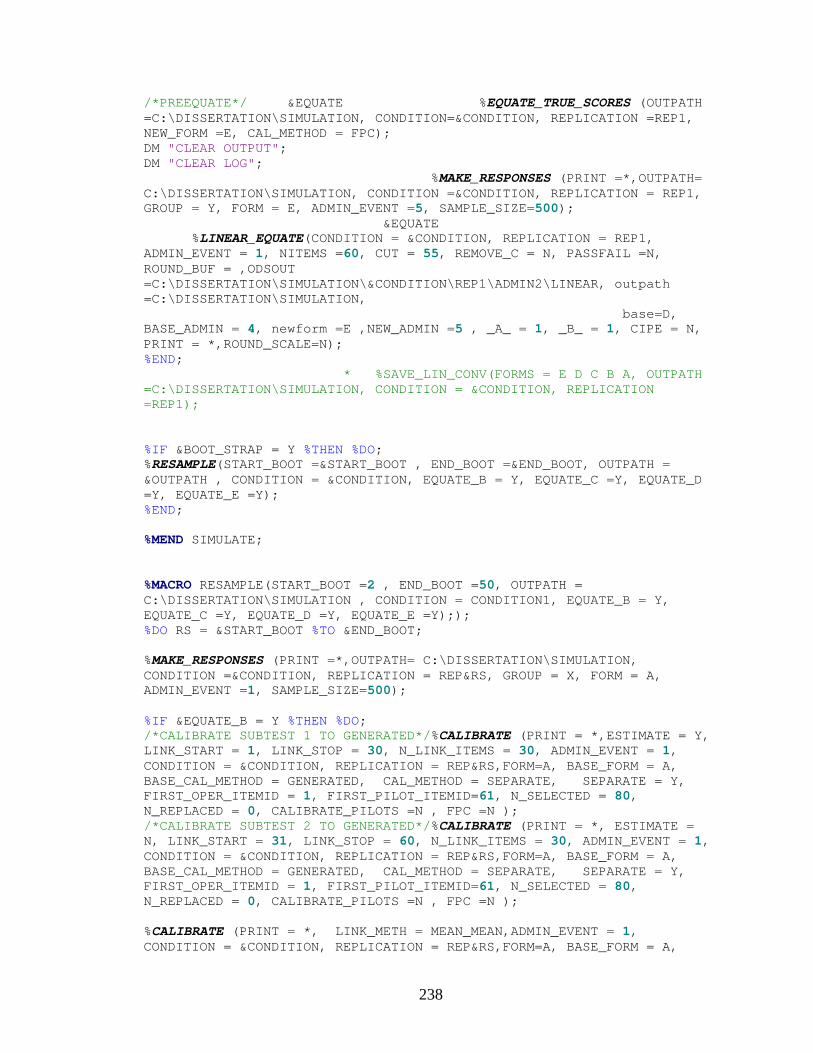
238

/*PREEQUATE*/ &EQUATE %EQUATE_TRUE_SCORES (OUTPATH =C:\DISSERTATION\SIMULATION, CONDITION=&CONDITION, REPLICATION =REP1, NEW_FORM =E, CAL_METHOD = FPC); DM "CLEAR OUTPUT"; DM "CLEAR LOG"; %MAKE_RESPONSES (PRINT =*,OUTPATH= C:\DISSERTATION\SIMULATION, CONDITION =&CONDITION, REPLICATION = REP1, GROUP = Y, FORM = E, ADMIN_EVENT =5, SAMPLE_SIZE=500); &EQUATE %LINEAR_EQUATE(CONDITION = &CONDITION, REPLICATION = REP1, ADMIN_EVENT = 1, NITEMS =60, CUT = 55, REMOVE_C = N, PASSFAIL =N, ROUND_BUF = ,ODSOUT =C:\DISSERTATION\SIMULATION\&CONDITION\REP1\ADMIN2\LINEAR, outpath =C:\DISSERTATION\SIMULATION, base=D, BASE_ADMIN = 4, newform =E ,NEW_ADMIN =5 , _A_ = 1, _B_ = 1, CIPE = N, PRINT = *,ROUND_SCALE=N); %END; * %SAVE_LIN_CONV(FORMS = E D C B A, OUTPATH =C:\DISSERTATION\SIMULATION, CONDITION = &CONDITION, REPLICATION =REP1); %IF &BOOT_STRAP = Y %THEN %DO; %RESAMPLE(START_BOOT =&START_BOOT , END_BOOT =&END_BOOT, OUTPATH = &OUTPATH , CONDITION = &CONDITION, EQUATE_B = Y, EQUATE_C =Y, EQUATE_D =Y, EQUATE_E =Y); %END; %MEND SIMULATE; %MACRO RESAMPLE(START_BOOT =2 , END_BOOT =50, OUTPATH = C:\DISSERTATION\SIMULATION , CONDITION = CONDITION1, EQUATE_B = Y, EQUATE_C =Y, EQUATE_D =Y, EQUATE_E =Y);); %DO RS = &START_BOOT %TO &END_BOOT; %MAKE_RESPONSES (PRINT =*,OUTPATH= C:\DISSERTATION\SIMULATION, CONDITION =&CONDITION, REPLICATION = REP&RS, GROUP = X, FORM = A, ADMIN_EVENT =1, SAMPLE_SIZE=500); %IF &EQUATE_B = Y %THEN %DO; /*CALIBRATE SUBTEST 1 TO GENERATED*/%CALIBRATE (PRINT = *,ESTIMATE = Y, LINK_START = 1, LINK_STOP = 30, N_LINK_ITEMS = 30, ADMIN_EVENT = 1, CONDITION = &CONDITION, REPLICATION = REP&RS,FORM=A, BASE_FORM = A, BASE_CAL_METHOD = GENERATED, CAL_METHOD = SEPARATE, SEPARATE = Y, FIRST_OPER_ITEMID = 1, FIRST_PILOT_ITEMID=61, N_SELECTED = 80, N_REPLACED = 0, CALIBRATE_PILOTS =N , FPC =N ); /*CALIBRATE SUBTEST 2 TO GENERATED*/%CALIBRATE (PRINT = *, ESTIMATE = N, LINK_START = 31, LINK_STOP = 60, N_LINK_ITEMS = 30, ADMIN_EVENT = 1, CONDITION = &CONDITION, REPLICATION = REP&RS,FORM=A, BASE_FORM = A, BASE_CAL_METHOD = GENERATED, CAL_METHOD = SEPARATE, SEPARATE = Y, FIRST_OPER_ITEMID = 1, FIRST_PILOT_ITEMID=61, N_SELECTED = 80, N_REPLACED = 0, CALIBRATE_PILOTS =N , FPC =N ); %CALIBRATE (PRINT = *, LINK_METH = MEAN_MEAN,ADMIN_EVENT = 1, CONDITION = &CONDITION, REPLICATION = REP&RS,FORM=A, BASE_FORM = A,

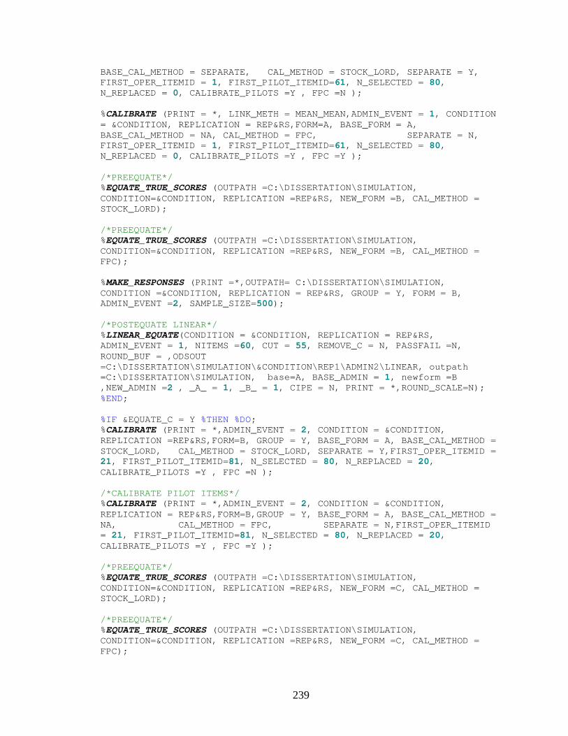
239

BASE_CAL_METHOD = SEPARATE, CAL_METHOD = STOCK_LORD, SEPARATE = Y, FIRST_OPER_ITEMID = 1, FIRST_PILOT_ITEMID=61, N_SELECTED = 80, N_REPLACED = 0, CALIBRATE_PILOTS =Y , FPC =N ); %CALIBRATE (PRINT = *, LINK_METH = MEAN_MEAN,ADMIN_EVENT = 1, CONDITION = &CONDITION, REPLICATION = REP&RS,FORM=A, BASE_FORM = A, BASE_CAL_METHOD = NA, CAL_METHOD = FPC, SEPARATE = N, FIRST_OPER_ITEMID = 1, FIRST_PILOT_ITEMID=61, N_SELECTED = 80, N_REPLACED = 0, CALIBRATE_PILOTS =Y , FPC =Y ); /*PREEQUATE*/ %EQUATE_TRUE_SCORES (OUTPATH =C:\DISSERTATION\SIMULATION, CONDITION=&CONDITION, REPLICATION =REP&RS, NEW_FORM =B, CAL_METHOD = STOCK_LORD); /*PREEQUATE*/ %EQUATE_TRUE_SCORES (OUTPATH =C:\DISSERTATION\SIMULATION, CONDITION=&CONDITION, REPLICATION =REP&RS, NEW_FORM =B, CAL_METHOD = FPC); %MAKE_RESPONSES (PRINT =*,OUTPATH= C:\DISSERTATION\SIMULATION, CONDITION =&CONDITION, REPLICATION = REP&RS, GROUP = Y, FORM = B, ADMIN_EVENT =2, SAMPLE_SIZE=500); /*POSTEQUATE LINEAR*/ %LINEAR_EQUATE(CONDITION = &CONDITION, REPLICATION = REP&RS, ADMIN_EVENT = 1, NITEMS =60, CUT = 55, REMOVE_C = N, PASSFAIL =N, ROUND_BUF = ,ODSOUT =C:\DISSERTATION\SIMULATION\&CONDITION\REP1\ADMIN2\LINEAR, outpath =C:\DISSERTATION\SIMULATION, base=A, BASE_ADMIN = 1, newform =B ,NEW_ADMIN =2 , _A_ = 1, _B_ = 1, CIPE = N, PRINT = *,ROUND_SCALE=N); %END; %IF &EQUATE_C = Y %THEN %DO; %CALIBRATE (PRINT = *,ADMIN_EVENT = 2, CONDITION = &CONDITION, REPLICATION =REP&RS,FORM=B, GROUP = Y, BASE_FORM = A, BASE_CAL_METHOD = STOCK_LORD, CAL_METHOD = STOCK_LORD, SEPARATE = Y,FIRST_OPER_ITEMID = 21, FIRST_PILOT_ITEMID=81, N_SELECTED = 80, N_REPLACED = 20, CALIBRATE_PILOTS =Y , FPC =N ); /*CALIBRATE PILOT ITEMS*/ %CALIBRATE (PRINT = *,ADMIN_EVENT = 2, CONDITION = &CONDITION, REPLICATION = REP&RS,FORM=B,GROUP = Y, BASE_FORM = A, BASE_CAL_METHOD = NA, CAL_METHOD = FPC, SEPARATE = N,FIRST_OPER_ITEMID = 21, FIRST_PILOT_ITEMID=81, N_SELECTED = 80, N_REPLACED = 20, CALIBRATE_PILOTS =Y , FPC =Y ); /*PREEQUATE*/ %EQUATE_TRUE_SCORES (OUTPATH =C:\DISSERTATION\SIMULATION, CONDITION=&CONDITION, REPLICATION =REP&RS, NEW_FORM =C, CAL_METHOD = STOCK_LORD); /*PREEQUATE*/ %EQUATE_TRUE_SCORES (OUTPATH =C:\DISSERTATION\SIMULATION, CONDITION=&CONDITION, REPLICATION =REP&RS, NEW_FORM =C, CAL_METHOD = FPC);

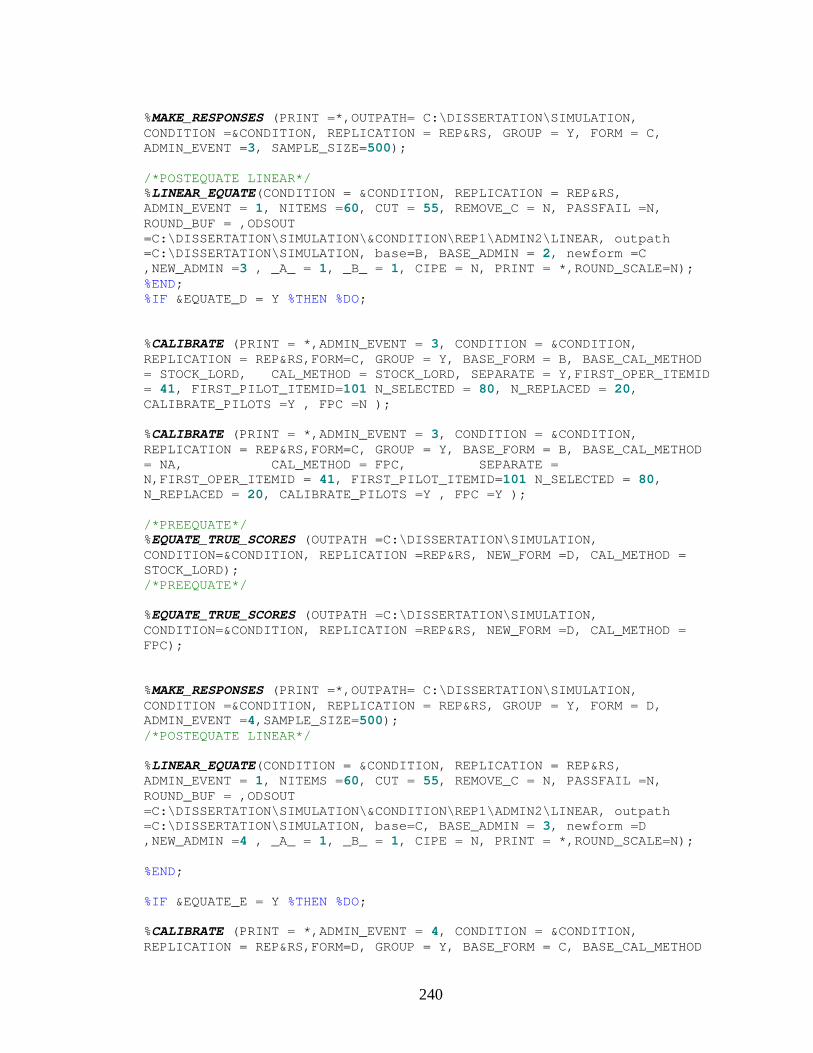
240

%MAKE_RESPONSES (PRINT =*,OUTPATH= C:\DISSERTATION\SIMULATION, CONDITION =&CONDITION, REPLICATION = REP&RS, GROUP = Y, FORM = C, ADMIN_EVENT =3, SAMPLE_SIZE=500); /*POSTEQUATE LINEAR*/ %LINEAR_EQUATE(CONDITION = &CONDITION, REPLICATION = REP&RS, ADMIN_EVENT = 1, NITEMS =60, CUT = 55, REMOVE_C = N, PASSFAIL =N, ROUND_BUF = ,ODSOUT =C:\DISSERTATION\SIMULATION\&CONDITION\REP1\ADMIN2\LINEAR, outpath =C:\DISSERTATION\SIMULATION, base=B, BASE_ADMIN = 2, newform =C ,NEW_ADMIN =3 , _A_ = 1, _B_ = 1, CIPE = N, PRINT = *,ROUND_SCALE=N); %END; %IF &EQUATE_D = Y %THEN %DO; %CALIBRATE (PRINT = *,ADMIN_EVENT = 3, CONDITION = &CONDITION, REPLICATION = REP&RS,FORM=C, GROUP = Y, BASE_FORM = B, BASE_CAL_METHOD = STOCK_LORD, CAL_METHOD = STOCK_LORD, SEPARATE = Y,FIRST_OPER_ITEMID = 41, FIRST_PILOT_ITEMID=101 N_SELECTED = 80, N_REPLACED = 20, CALIBRATE_PILOTS =Y , FPC =N ); %CALIBRATE (PRINT = *,ADMIN_EVENT = 3, CONDITION = &CONDITION, REPLICATION = REP&RS,FORM=C, GROUP = Y, BASE_FORM = B, BASE_CAL_METHOD = NA, CAL_METHOD = FPC, SEPARATE = N,FIRST_OPER_ITEMID = 41, FIRST_PILOT_ITEMID=101 N_SELECTED = 80, N_REPLACED = 20, CALIBRATE_PILOTS =Y , FPC =Y ); /*PREEQUATE*/ %EQUATE_TRUE_SCORES (OUTPATH =C:\DISSERTATION\SIMULATION, CONDITION=&CONDITION, REPLICATION =REP&RS, NEW_FORM =D, CAL_METHOD = STOCK_LORD); /*PREEQUATE*/ %EQUATE_TRUE_SCORES (OUTPATH =C:\DISSERTATION\SIMULATION, CONDITION=&CONDITION, REPLICATION =REP&RS, NEW_FORM =D, CAL_METHOD = FPC); %MAKE_RESPONSES (PRINT =*,OUTPATH= C:\DISSERTATION\SIMULATION, CONDITION =&CONDITION, REPLICATION = REP&RS, GROUP = Y, FORM = D, ADMIN_EVENT =4,SAMPLE_SIZE=500); /*POSTEQUATE LINEAR*/ %LINEAR_EQUATE(CONDITION = &CONDITION, REPLICATION = REP&RS, ADMIN_EVENT = 1, NITEMS =60, CUT = 55, REMOVE_C = N, PASSFAIL =N, ROUND_BUF = ,ODSOUT =C:\DISSERTATION\SIMULATION\&CONDITION\REP1\ADMIN2\LINEAR, outpath =C:\DISSERTATION\SIMULATION, base=C, BASE_ADMIN = 3, newform =D ,NEW_ADMIN =4 , _A_ = 1, _B_ = 1, CIPE = N, PRINT = *,ROUND_SCALE=N); %END; %IF &EQUATE_E = Y %THEN %DO; %CALIBRATE (PRINT = *,ADMIN_EVENT = 4, CONDITION = &CONDITION, REPLICATION = REP&RS,FORM=D, GROUP = Y, BASE_FORM = C, BASE_CAL_METHOD

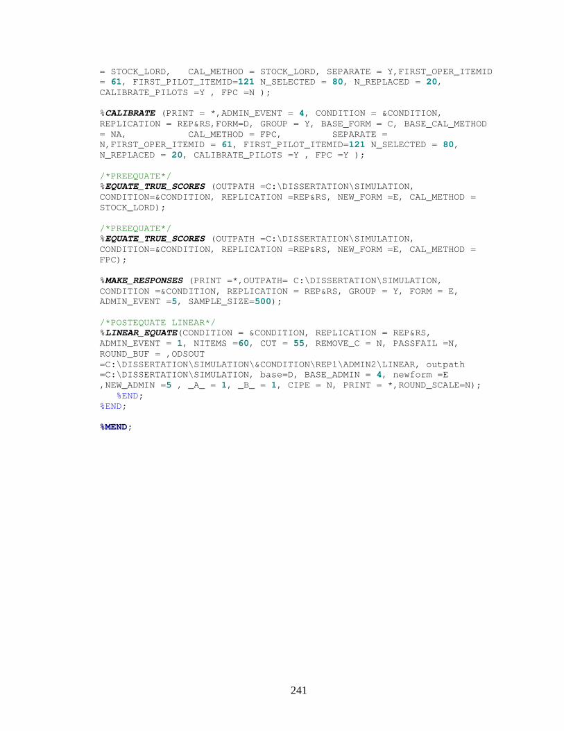
241

= STOCK_LORD, CAL_METHOD = STOCK_LORD, SEPARATE = Y,FIRST_OPER_ITEMID = 61, FIRST_PILOT_ITEMID=121 N_SELECTED = 80, N_REPLACED = 20, CALIBRATE_PILOTS =Y , FPC =N ); %CALIBRATE (PRINT = *,ADMIN_EVENT = 4, CONDITION = &CONDITION, REPLICATION = REP&RS,FORM=D, GROUP = Y, BASE_FORM = C, BASE_CAL_METHOD = NA, CAL_METHOD = FPC, SEPARATE = N,FIRST_OPER_ITEMID = 61, FIRST_PILOT_ITEMID=121 N_SELECTED = 80, N_REPLACED = 20, CALIBRATE_PILOTS =Y , FPC =Y ); /*PREEQUATE*/ %EQUATE_TRUE_SCORES (OUTPATH =C:\DISSERTATION\SIMULATION, CONDITION=&CONDITION, REPLICATION =REP&RS, NEW_FORM =E, CAL_METHOD = STOCK_LORD); /*PREEQUATE*/ %EQUATE_TRUE_SCORES (OUTPATH =C:\DISSERTATION\SIMULATION, CONDITION=&CONDITION, REPLICATION =REP&RS, NEW_FORM =E, CAL_METHOD = FPC); %MAKE_RESPONSES (PRINT =*,OUTPATH= C:\DISSERTATION\SIMULATION, CONDITION =&CONDITION, REPLICATION = REP&RS, GROUP = Y, FORM = E, ADMIN_EVENT =5, SAMPLE_SIZE=500); /*POSTEQUATE LINEAR*/ %LINEAR_EQUATE(CONDITION = &CONDITION, REPLICATION = REP&RS, ADMIN_EVENT = 1, NITEMS =60, CUT = 55, REMOVE_C = N, PASSFAIL =N, ROUND_BUF = ,ODSOUT =C:\DISSERTATION\SIMULATION\&CONDITION\REP1\ADMIN2\LINEAR, outpath =C:\DISSERTATION\SIMULATION, base=D, BASE_ADMIN = 4, newform =E ,NEW_ADMIN =5 , _A_ = 1, _B_ = 1, CIPE = N, PRINT = *,ROUND_SCALE=N); %END; %END; %MEND;

242

APPENDIX B: DESCRIPTIVE STATISTICS OF GENERATED TEST FORMS

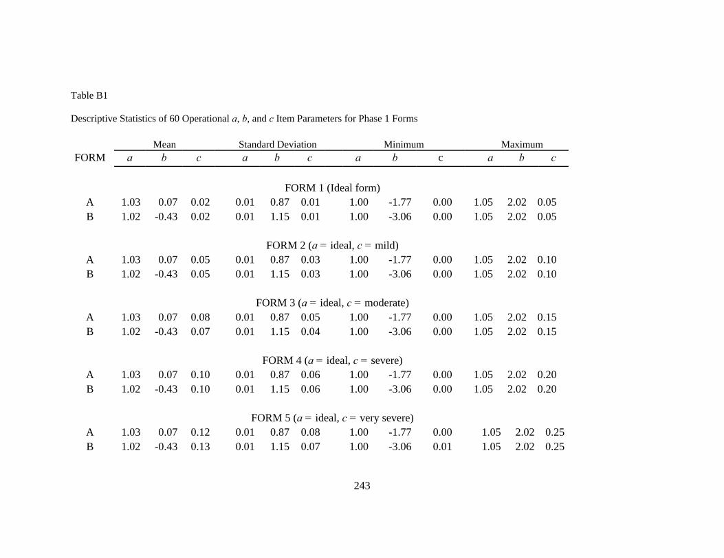
243

Table B1 Descriptive Statistics of 60 Operational a, b, and c Item Parameters for Phase 1 Forms Mean Standard Deviation Minimum Maximum FORM a b c a b c a b c a b c

FORM 1 (Ideal form) A 1.03 0.07 0.02 0.01 0.87 0.01 1.00 -1.77 0.00 1.05 2.02 0.05B 1.02 -0.43 0.02 0.01 1.15 0.01 1.00 -3.06 0.00 1.05 2.02 0.05 FORM 2 (a = ideal, c = mild) A 1.03 0.07 0.05 0.01 0.87 0.03 1.00 -1.77 0.00 1.05 2.02 0.10B 1.02 -0.43 0.05 0.01 1.15 0.03 1.00 -3.06 0.00 1.05 2.02 0.10 FORM 3 (a = ideal, c = moderate) A 1.03 0.07 0.08 0.01 0.87 0.05 1.00 -1.77 0.00 1.05 2.02 0.15B 1.02 -0.43 0.07 0.01 1.15 0.04 1.00 -3.06 0.00 1.05 2.02 0.15 FORM 4 (a = ideal, c = severe) A 1.03 0.07 0.10 0.01 0.87 0.06 1.00 -1.77 0.00 1.05 2.02 0.20B 1.02 -0.43 0.10 0.01 1.15 0.06 1.00 -3.06 0.00 1.05 2.02 0.20 FORM 5 (a = ideal, c = very severe) A 1.03 0.07 0.12 0.01 0.87 0.08 1.00 -1.77 0.00 1.05 2.02 0.25B 1.02 -0.43 0.13 0.01 1.15 0.07 1.00 -3.06 0.01 1.05 2.02 0.25

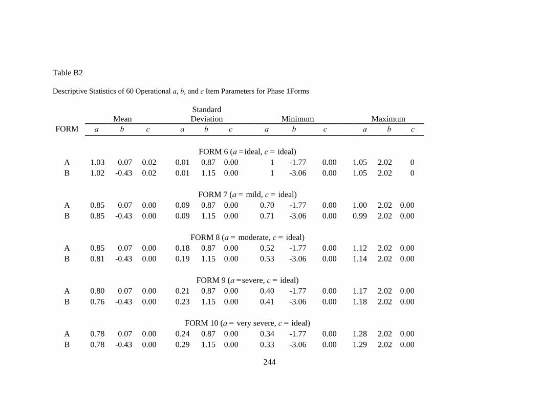
244

Table B2 Descriptive Statistics of 60 Operational a, b, and c Item Parameters for Phase 1Forms

Mean Standard Deviation Minimum Maximum

FORM a b c a b c a b c a b c FORM 6 (a =ideal, c = ideal) A 1.03 0.07 0.02 0.01 0.87 0.00 1 -1.77 0.00 1.05 2.02 0B 1.02 -0.43 0.02 0.01 1.15 0.00 1 -3.06 0.00 1.05 2.02 0

FORM 7 (a = mild, c = ideal) A 0.85 0.07 0.00 0.09 0.87 0.00 0.70 -1.77 0.00 1.00 2.02 0.00B 0.85 -0.43 0.00 0.09 1.15 0.00 0.71 -3.06 0.00 0.99 2.02 0.00 FORM 8 (a = moderate, c = ideal) A 0.85 0.07 0.00 0.18 0.87 0.00 0.52 -1.77 0.00 1.12 2.02 0.00B 0.81 -0.43 0.00 0.19 1.15 0.00 0.53 -3.06 0.00 1.14 2.02 0.00 FORM 9 (a =severe, c = ideal) A 0.80 0.07 0.00 0.21 0.87 0.00 0.40 -1.77 0.00 1.17 2.02 0.00B 0.76 -0.43 0.00 0.23 1.15 0.00 0.41 -3.06 0.00 1.18 2.02 0.00 FORM 10 (a = very severe, c = ideal) A 0.78 0.07 0.00 0.24 0.87 0.00 0.34 -1.77 0.00 1.28 2.02 0.00B 0.78 -0.43 0.00 0.29 1.15 0.00 0.33 -3.06 0.00 1.29 2.02 0.00

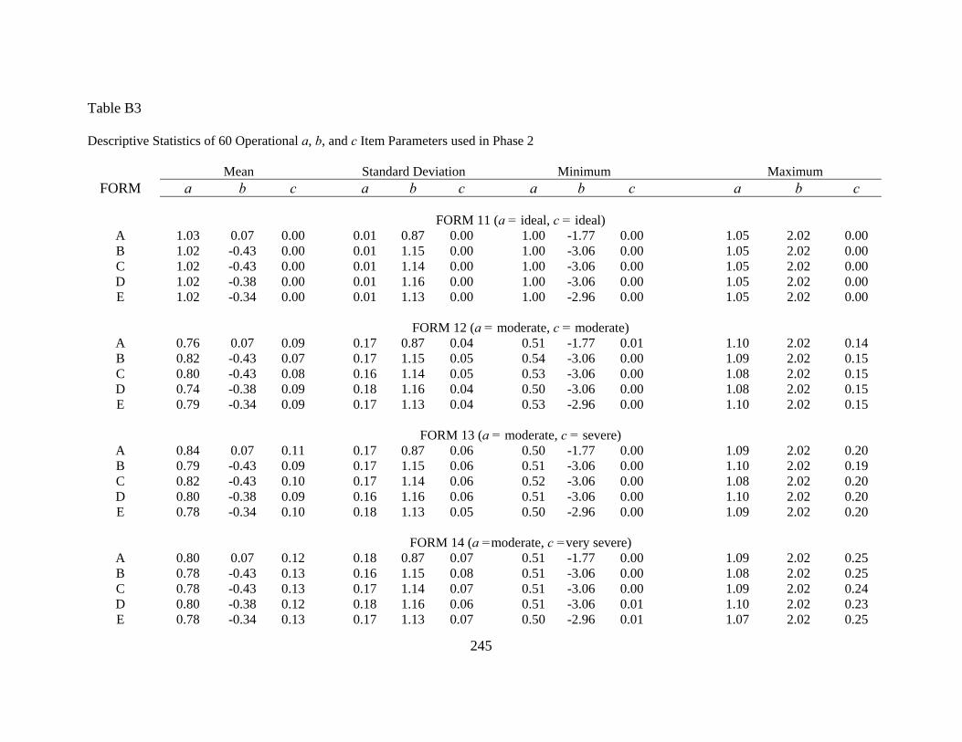
245

Table B3 Descriptive Statistics of 60 Operational a, b, and c Item Parameters used in Phase 2 Mean Standard Deviation Minimum Maximum

FORM a b c a b c a b c a b c FORM 11 (a = ideal, c = ideal) A 1.03 0.07 0.00 0.01 0.87 0.00 1.00 -1.77 0.00 1.05 2.02 0.00 B 1.02 -0.43 0.00 0.01 1.15 0.00 1.00 -3.06 0.00 1.05 2.02 0.00 C 1.02 -0.43 0.00 0.01 1.14 0.00 1.00 -3.06 0.00 1.05 2.02 0.00 D 1.02 -0.38 0.00 0.01 1.16 0.00 1.00 -3.06 0.00 1.05 2.02 0.00 E 1.02 -0.34 0.00 0.01 1.13 0.00 1.00 -2.96 0.00 1.05 2.02 0.00 FORM 12 (a = moderate, c = moderate) A 0.76 0.07 0.09 0.17 0.87 0.04 0.51 -1.77 0.01 1.10 2.02 0.14 B 0.82 -0.43 0.07 0.17 1.15 0.05 0.54 -3.06 0.00 1.09 2.02 0.15 C 0.80 -0.43 0.08 0.16 1.14 0.05 0.53 -3.06 0.00 1.08 2.02 0.15 D 0.74 -0.38 0.09 0.18 1.16 0.04 0.50 -3.06 0.00 1.08 2.02 0.15 E 0.79 -0.34 0.09 0.17 1.13 0.04 0.53 -2.96 0.00 1.10 2.02 0.15 FORM 13 (a = moderate, c = severe) A 0.84 0.07 0.11 0.17 0.87 0.06 0.50 -1.77 0.00 1.09 2.02 0.20 B 0.79 -0.43 0.09 0.17 1.15 0.06 0.51 -3.06 0.00 1.10 2.02 0.19 C 0.82 -0.43 0.10 0.17 1.14 0.06 0.52 -3.06 0.00 1.08 2.02 0.20 D 0.80 -0.38 0.09 0.16 1.16 0.06 0.51 -3.06 0.00 1.10 2.02 0.20 E 0.78 -0.34 0.10 0.18 1.13 0.05 0.50 -2.96 0.00 1.09 2.02 0.20 FORM 14 (a =moderate, c =very severe) A 0.80 0.07 0.12 0.18 0.87 0.07 0.51 -1.77 0.00 1.09 2.02 0.25 B 0.78 -0.43 0.13 0.16 1.15 0.08 0.51 -3.06 0.00 1.08 2.02 0.25 C 0.78 -0.43 0.13 0.17 1.14 0.07 0.51 -3.06 0.00 1.09 2.02 0.24 D 0.80 -0.38 0.12 0.18 1.16 0.06 0.51 -3.06 0.01 1.10 2.02 0.23 E 0.78 -0.34 0.13 0.17 1.13 0.07 0.50 -2.96 0.01 1.07 2.02 0.25

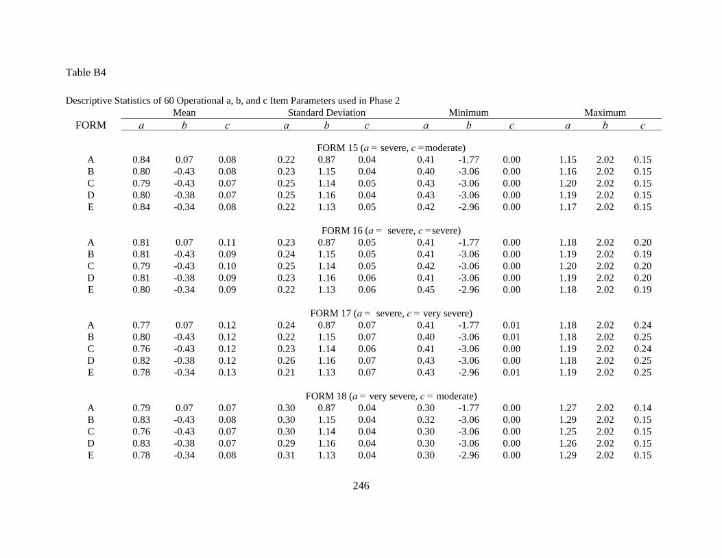
246

Table B4

Descriptive Statistics of 60 Operational a, b, and c Item Parameters used in Phase 2 Mean Standard Deviation Minimum Maximum

FORM a b c a b c a b c a b c FORM 15 (a = severe, c =moderate) A 0.84 0.07 0.08 0.22 0.87 0.04 0.41 -1.77 0.00 1.15 2.02 0.15 B 0.80 -0.43 0.08 0.23 1.15 0.04 0.40 -3.06 0.00 1.16 2.02 0.15 C 0.79 -0.43 0.07 0.25 1.14 0.05 0.43 -3.06 0.00 1.20 2.02 0.15 D 0.80 -0.38 0.07 0.25 1.16 0.04 0.43 -3.06 0.00 1.19 2.02 0.15 E 0.84 -0.34 0.08 0.22 1.13 0.05 0.42 -2.96 0.00 1.17 2.02 0.15 FORM 16 (a = severe, c =severe) A 0.81 0.07 0.11 0.23 0.87 0.05 0.41 -1.77 0.00 1.18 2.02 0.20 B 0.81 -0.43 0.09 0.24 1.15 0.05 0.41 -3.06 0.00 1.19 2.02 0.19 C 0.79 -0.43 0.10 0.25 1.14 0.05 0.42 -3.06 0.00 1.20 2.02 0.20 D 0.81 -0.38 0.09 0.23 1.16 0.06 0.41 -3.06 0.00 1.19 2.02 0.20 E 0.80 -0.34 0.09 0.22 1.13 0.06 0.45 -2.96 0.00 1.18 2.02 0.19 FORM 17 (a = severe, c = very severe) A 0.77 0.07 0.12 0.24 0.87 0.07 0.41 -1.77 0.01 1.18 2.02 0.24 B 0.80 -0.43 0.12 0.22 1.15 0.07 0.40 -3.06 0.01 1.18 2.02 0.25 C 0.76 -0.43 0.12 0.23 1.14 0.06 0.41 -3.06 0.00 1.19 2.02 0.24 D 0.82 -0.38 0.12 0.26 1.16 0.07 0.43 -3.06 0.00 1.18 2.02 0.25 E 0.78 -0.34 0.13 0.21 1.13 0.07 0.43 -2.96 0.01 1.19 2.02 0.25 FORM 18 (a = very severe, c = moderate) A 0.79 0.07 0.07 0.30 0.87 0.04 0.30 -1.77 0.00 1.27 2.02 0.14 B 0.83 -0.43 0.08 0.30 1.15 0.04 0.32 -3.06 0.00 1.29 2.02 0.15 C 0.76 -0.43 0.07 0.30 1.14 0.04 0.30 -3.06 0.00 1.25 2.02 0.15 D 0.83 -0.38 0.07 0.29 1.16 0.04 0.30 -3.06 0.00 1.26 2.02 0.15 E 0.78 -0.34 0.08 0.31 1.13 0.04 0.30 -2.96 0.00 1.29 2.02 0.15

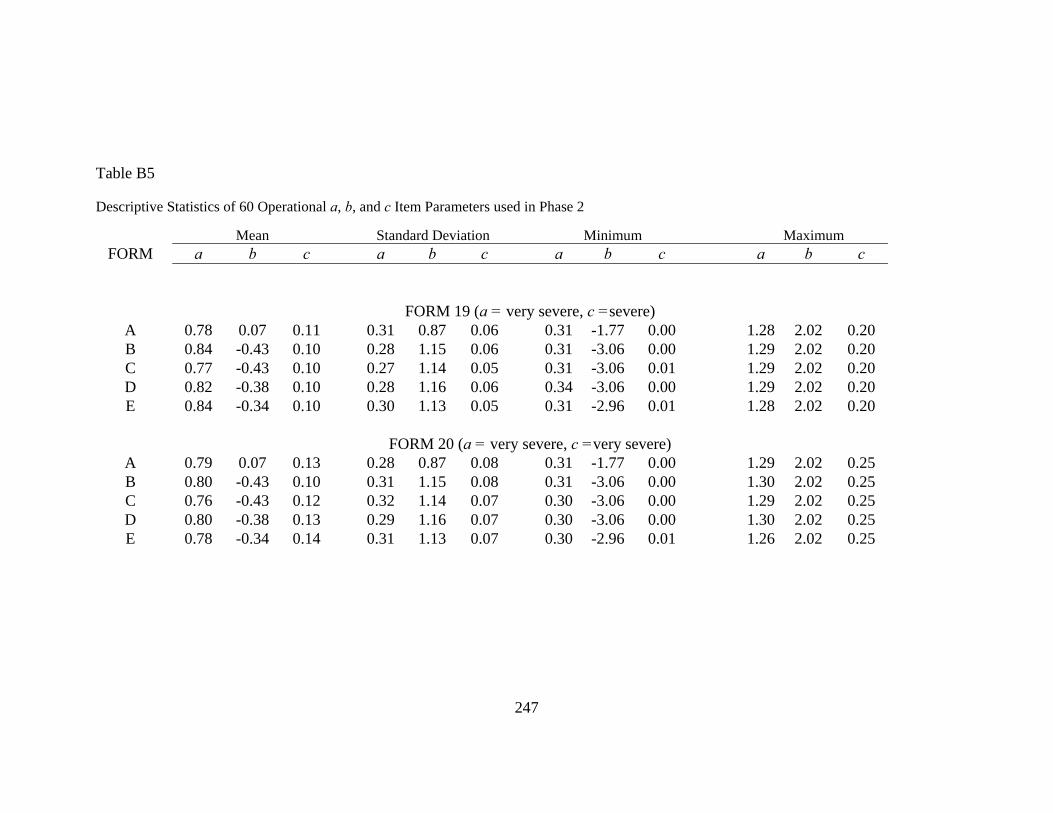
247

Table B5

Descriptive Statistics of 60 Operational a, b, and c Item Parameters used in Phase 2

Mean Standard Deviation Minimum Maximum FORM a b c a b c a b c a b c

FORM 19 (a = very severe, c =severe) A 0.78 0.07 0.11 0.31 0.87 0.06 0.31 -1.77 0.00 1.28 2.02 0.20 B 0.84 -0.43 0.10 0.28 1.15 0.06 0.31 -3.06 0.00 1.29 2.02 0.20 C 0.77 -0.43 0.10 0.27 1.14 0.05 0.31 -3.06 0.01 1.29 2.02 0.20 D 0.82 -0.38 0.10 0.28 1.16 0.06 0.34 -3.06 0.00 1.29 2.02 0.20 E 0.84 -0.34 0.10 0.30 1.13 0.05 0.31 -2.96 0.01 1.28 2.02 0.20 FORM 20 (a = very severe, c =very severe) A 0.79 0.07 0.13 0.28 0.87 0.08 0.31 -1.77 0.00 1.29 2.02 0.25 B 0.80 -0.43 0.10 0.31 1.15 0.08 0.31 -3.06 0.00 1.30 2.02 0.25 C 0.76 -0.43 0.12 0.32 1.14 0.07 0.30 -3.06 0.00 1.29 2.02 0.25 D 0.80 -0.38 0.13 0.29 1.16 0.07 0.30 -3.06 0.00 1.30 2.02 0.25 E 0.78 -0.34 0.14 0.31 1.13 0.07 0.30 -2.96 0.01 1.26 2.02 0.25

248

APPENDIX C: DESCRIPTIVE STATISTICS FOR GENERATED THETA DISTRIBUTIONS

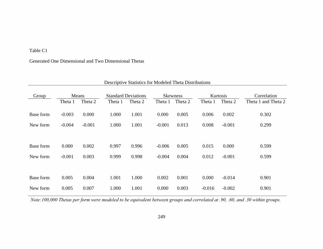
249

Table C1

Generated One Dimensional and Two Dimensional Thetas

Descriptive Statistics for Modeled Theta Distributions

Group Means Standard Deviations Skewness Kurtosis Correlation Theta 1 Theta 2 Theta 1 Theta 2 Theta 1 Theta 2 Theta 1 Theta 2 Theta 1 and Theta 2

Base form -0.003 0.000 1.000 1.001 0.000 0.005 0.006 0.002 0.302

New form -0.004 -0.001 1.000 1.001 -0.001 0.013 0.008 -0.001 0.299

Base form 0.000 0.002 0.997 0.996 -0.006 0.005 0.015 0.000 0.599

New form -0.001 0.003 0.999 0.998 -0.004 0.004 0.012 -0.001 0.599

Base form 0.005 0.004 1.001 1.000 0.002 0.001 0.000 -0.014 0.901

New form 0.005 0.007 1.000 1.001 0.000 0.003 -0.016 -0.002 0.901

Note:100,000 Thetas per form were modeled to be equivalent between groups and correlated at .90, .60, and .30 within groups.

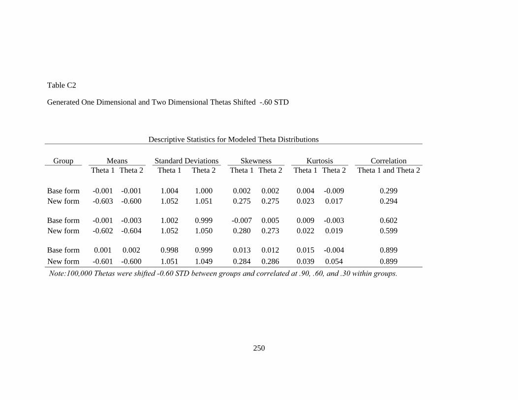
250

Table C2

Generated One Dimensional and Two Dimensional Thetas Shifted -.60 STD



Base form -0.001 -0.001 1.004 1.000 0.002 0.002 0.004 -0.009 0.299 New form -0.603 -0.600 1.052 1.051 0.275 0.275 0.023 0.017 0.294

Base form -0.001 -0.003 1.002 0.999 -0.007 0.005 0.009 -0.003 0.602 New form -0.602 -0.604 1.052 1.050 0.280 0.273 0.022 0.019 0.599

Base form 0.001 0.002 0.998 0.999 0.013 0.012 0.015 -0.004 0.899 New form -0.601 -0.600 1.051 1.049 0.284 0.286 0.039 0.054 0.899 Note:100,000 Thetas were shifted -0.60 STD between groups and correlated at .90, .60, and .30 within groups.

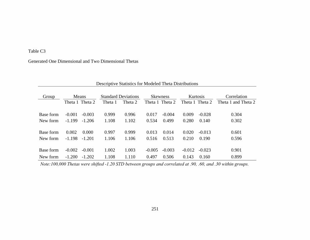
251

Table C3

Generated One Dimensional and Two Dimensional Thetas



Base form -0.001 -0.003 0.999 0.996 0.017 -0.004 0.009 -0.028 0.304 New form -1.199 -1.206 1.108 1.102 0.534 0.499 0.280 0.140 0.302

Base form 0.002 0.000 0.997 0.999 0.013 0.014 0.020 -0.013 0.601 New form -1.198 -1.201 1.106 1.106 0.516 0.513 0.210 0.190 0.596

Base form -0.002 -0.001 1.002 1.003 -0.005 -0.003 -0.012 -0.023 0.901 New form -1.200 -1.202 1.108 1.110 0.497 0.506 0.143 0.160 0.899 Note:100,000 Thetas were shifted -1.20 STD between groups and correlated at .90, .60, and .30 within groups.

ABOUT THE AUTHOR

Garron has worked as a psychometrician in the certification and licensing field

since 2005. He is currently employed as a psychometrician at Professional Testing, Inc.

in Orlando, Fl., where he is responsible for exam scoring, equating, and reporting.

Previous to that, he was employed as a psychometrician at the Institute for Instructional

Research and Practice at the University of South Florida. At the Institute, he was

responsible for the scoring, equating, and reporting of tests for the Florida Educational

Leadership Exam. In addition, he prepared technical reports for the Florida Teacher

Certification Exams. Garron has proficiency in Base SAS, SAS graph, and the SAS

macro language. His research interests include traditional and IRT equating, IRT item

calibration, and score reporting. Garron is married to Kristie and has a four year old

daughter, Eliana. He currently resides with his family in Raleigh, North Carolina.

Documents

The Robustness of Rasch True Score Preequating to