The role of aggregation technologies in the provision of

The role of aggregation technologies in the provision

of supranational public goods: A reconsideration of

NATO’s strategies.

Ghislain Dutheil

de la Rochère ∗

Jean-Michel Josselin † Yvon Rocaboy‡

Abstract

Voluntary contributions to the provision of public goods do not necessarily follow a

summation aggregation technology. The article investigates the alternative best-shot ag-

gregation process and provides the corresponding Nash equilibrium conditions for allies

in the context of joint products in a supranational alliance. The application deals with

NATO over the period 1955-2006 and evidences new breakpoints and aggregation tech-

nology assessments, which leads to a reconsideration of the alliance’s strategy. We find

that a best-shot technology prevails from 1955 to 1970. Afterwards, summation of con-

tributions becomes the aggregation technology of the alliance, with increased strategic

behavior after 1990.

JEL-Classification: D74 · H41 · H56 · H87

Keywords: Supranational public goods, International organizations, Aggregation of

contributions, Best-shot, NATO

∗Ecoles de Saint-Cyr Coëquidan and CREC, Guer, France. E-mail: [email protected]

†University of Rennes I and CREM-CNRS, Rennes, France. E-mail: [email protected]‡University of Rennes I and CREM-CNRS, Rennes, France. E-mail: [email protected]

1. Introduction

The provision of supranational public goods has become a subject of increasing concern for

collective action. It may relate to transnational health programs, protection against environ-

mental hazards, preservation of peace and security . . . and it involves formal or informal supra-

national organizations which implement the decisions reached by their contributors (Sandler,

2006). Our paper follows this track and it is dedicated to the study and assessment of NATO’s

strategy from 1955 to 2006. NATO’s strategy is interpreted here as the provision of a supra-

national public good whose nature and properties can vary during the period of study.

Members of NATO are sovereign states and they are modeled here as individual agents

in a static and non cooperative game of voluntary contributions (Warr 1983; Cornes and San-

dler 1984; Bergstrom et al. 1986). In this setting, contributions to the supranational public

good are usually aggregated by a summation technology, following the founding articles of

Samuelson (1954, 1955). Studies of NATO have used it, particularly the pioneering work of

Olson and Zeckhauser (1966), which has triggered a vast literature surveyed by Sandler and

Hartley (2001). Olson and Zeckhauser (1966) used a pure public good model that was later

complemented with the joint product model of Sandler (1977). This literature has identified

a first period (1949-1967) when the doctrine of "mutual assured destruction" (as it is formal-

ized by NATO’s directive MC48 in 1954) yields a pure supranational public good. A second

period begins with the "flexible response doctrine" (NATO’s directive MC14/3). The alliance

now provides joint products. In both cases, sub-optimality of Nash equilibria is evidenced

and it also triggers a heated debate on the so-called "exploitation hypothesis" by which small

members of the alliance would free ride on the biggest contributor, namely the United States.

From 1991 onwards, the "crisis management doctrine" prevails. The exploitation debate

somewhat fades away, but new challenges arise. Europe and the world’s security and stability

amount to purely public benefits (Sandler and Hartley 2001), which increases the share of

2

pure public outputs in NATO’s activities as well as free-riding opportunities.

Intuitively, even if the previous theoretical setting is path-breaking, it may not be able

to comprehend the variety of situations that can be faced when economic agents (either in-

dividuals or states) decide to engage into collective action. In particular, the technology of

aggregation of contributions may not always be as straightforward as that of summation. The

situation may be so that the weakest contribution drags down the level of provided public

good. Conversely, one agent may have such a prominent contribution that no other prevails,

at least in static terms. In other words, the technology of aggregation of contributions matters.

It does so in two respects.

First, from a theoretical viewpoint, Nash equilibrium conditions are likely to differ from

what they are in the standard summation setting. The systematic study of technologies of ag-

gregation of contributions to public goods can be dated back to the seminal work of Hirshleifer

(1983, 1985). Hirshleifer provides a thought-provoking intuitive analysis, using vivid exam-

ples and providing a diagrammatic illustration of the summation and weakest-link cases (see

also Cornes 1993). The early results of Hirshleifer have recently been systematized by Cornes

and Hartley (2007) in the context of the provision of a pure public good (for an approach with

incomplete information see also Xu 2001).

Second, in empirical terms, alternative technologies of aggregation matter all the more

that they may provide a much more accurate illumination of facts. There are very few studies

explicitly using such alternatives. A good example is for instance Conybeare et al. (1994)

who compare the explanatory power of the weakest-link and best-shot technologies mainly in

the case of pre-WWI alliances.

Our contribution to the theoretical and empirical landscape that has just been described is

the following. In theoretical terms, we consider here the joint product model with alternative

aggregation technologies. Most if not all NATO members have always kept their own "private"

defense agenda, with for instance regional or colonial interests or internal security constraints.

3

Furthermore, national conventional forces can be deployed along an alliance’s perimeter or

they can join combined task forces. The joint product model thus seems to more adequately

fit the objectives and constraints of the allies.

Nash equilibrium conditions have been provided by Sandler (1977) in the summation case

and by Conybeare et al. (1994) in the best-shot case. We provide a concise presentation

of both. In empirical terms, we use panel data for the first time (to our knowledge) over an

extended horizon (1955-2006). Contrary to Gadea et al. (2004) who test unknown breakpoints

with a summation technology in a time series framework, we test competing technologies that

are relevant in the NATO case, namely summation and best-shot, with unknown breakpoints

in a panel data framework. The case of a weakest link could have been envisaged, at least in

theoretical terms. However, the empirical framework of deterrence, whether or not mitigated

by potential conventional conflict, does not plead in favor of this aggregation technology.

Deterrence is indeed characterized by a global defense strategy as opposed to what Hirshleifer

(1983: 372) labels a “linear” situation where each member of the alliance is responsible for

one link of a chain. In other historical circumstances, this weakest-link situation has been

proved relevant. For instance, Conybeare et al. (1994) and Conybeare and Sandler (1990)

have shown that the United Kingdom was the weakest-link of the Triple Entente in the World

War I conflict. The Cold War context is quite different.

We find that best-shot rather than summation is relevant from 1955 to 1970. Year 1967

is often regarded as the end of the first period (Sandler and Forbes 1980; Oneal and Elrod

1989; Khanna and Sandler 1996). Our estimations thus reject this date.1 They confirm the

summation technology from 1971 to 2006, but they identify an increase in strategic behaviors

after 1990. Summation can indeed be associated with the opportunistic behavior of allies

intending to shift the defense burden on the others. This kind of "free-riding" intensifies after

1Admittedly, Sandler and Murdoch (2000) do not consider the 1967 date as a study result but use it as aninstitutional landmark. Others do not take it as given in their econometric investigations (for instance Gadea etal. 2004)

4

1990. All these results provide a significant reconsideration of NATO’s strategies in the long

run.

The article is organized as follows. Section 2 describes the theoretical framework. Sec-

tion 3 presents the empirical results, followed by concluding comments and discussion in

section 4.

2. Provision of joint products in an alliance under summation or best-

shot technologies

We first present a model of joint products in an alliance, allowing summation or best-shot

technologies (section 2.1). We then specify the Nash equilibrium conditions in both cases

(section 2.2).

2.1. Joint products under summation or best-shot

Consider an alliance consisting of countries i = 1, . . . ,n. Membership implies contributing

to the supranational public good G provided by the alliance. Allies have initial endowments

yi and their utility functions comprise the consumption of a numéraire in quantity xi. The

expression of utility functions then depends on the type of public good provided by the al-

liance. In the Olson and Zeckhauser (1966) framework, G is a pure public good, so that

ui = ui(xi,G). With the joint product approach suggested by Sandler (1977) and adopted here,

the ally’s global military activity qi comprehends a contribution to the alliance-wide deter-

rence G and an ally-specific local public good. To give an illustration, GDP yi of the allied

country is in part used for the consumption xi of its citizens, possibly including the provision

of non-military national public goods. The complement qi is used for conventional and tacti-

cal weapons aiming at the direct protection of its national interests, and for contributing to the

stockpile of strategic weapons G on which the alliance’s defense policy is built. In the joint

product case, the utility function is thus ui = ui(xi,qi,G).

5

Following Cornes and Sandler (1996), the aggregation technologies of contribution can be

synthesized by

G = G(q1, . . . ,qi, . . . ,qn) = φ

(1n

n

∑i=1

qνi

) 1ν

(1)

Different values of parameters φ and ν define specific technologies.2 Among them, summa-

tion is such that

φ = n and ν = 1⇒ G = G(q1, . . . ,qi, . . . ,qn) =n

∑i=1

qi (2)

Best shot is defined by

φ = 1 and ν =+∞⇒ G = G(q1, . . . ,qi, . . . ,qn)→maxi(q1, . . . ,qi, . . . ,qn) (3)

The largest contribution defines the aggregate level of public good.

2.2. Nash equilibrium conditions

First, we consider the case of a summation aggregation technology (Cornes and Sandler 1984).

With p the unit price of defense activity and the unit price of xi set at 1, the Nash program of

a given contributor i is

maxxi,qi;i=1,...,n

ui = ui(xi,qi,G) subject to xi + pqi = yi (4)

where G = G(q1, . . . ,qi, . . . ,qn) = ∑ni=1 qi

2We do not consider the weakest link, which is given by

φ = 1 and ν =−∞⇒ G = G(q1, . . . ,qi, . . . ,qn)→mini(q1, . . . ,qi, . . . ,qn)

The smallest contribution sets the aggregate level of public good.

6

Using the first order conditions, we get

∂ui (yi− pqi,qi,G)

∂qi∂ui (yi− pqi,qi,G)

∂xi

+


∂G∂ui (yi− pqi,qi,G)

∂xi

= p (5)

The Nash equilibrium condition for country i can thus be expressed as

qi = fi (G−i,yi, p) (6)

where G−i is the total defense expenditures of the alliance minus those of country i.

We then move on to the best-shot case (Conybeare et al. 1994), for which the Nash

program of a given member state is the same as 4 but where G = G(q1, . . . ,qi, . . . ,qn) =(1n

∑ni=1 qν

i

) 1ν

and ν =+∞.

Using the first order conditions we obtain


∂qi∂ui (yi− pqi,qi,G)

∂xi

+


∂G∂ui (yi− pqi,qi,G)

∂xi

∂G∂qi

= p (7)

Deriving equation 1 with respect to qi gives

∂G∂qi→(

1n

) 1ν

1(q1

qi

)ν

+ . . .+1+ . . .+

(qn

qi

)ν

1− 1

ν

(8)

For a best-shot technology, ν =+∞. Equation 8 becomes

∂G∂qi→

1(q1

qi

)∞

+ . . .+1+ . . .+

(qn

qi

)∞

(9)

7

If qi = qmax, then∂G

∂qmax→ 1. Otherwise, if qi 6= qmax, then

∂G∂qi→ 0.

If qi 6= qmax, country i is not the best-shot ally. Using equation 7, its Nash equilibrium

condition can be written as

qi = fi (Gmax,yi, p) (10)

where Gmax represents the defense expenditures of the best-shot ally.

If qi = qmax, country i is the best-shot ally. We proceed in a similar way to obtain its Nash

equilibrium condition

qmax = fmax (ymax, p) (11)

We now propose to apply the previous framework to the assessment of NATO’s policies over

the last six decades.

3. Application to NATO

3.1. Presentation and preliminary analysis of the data set

The study goes over 1955-2006. The first years of NATO (1949-1954) are not included since

they are mostly a set-up period. Year 1955 also marks the entry of Germany in the alliance.

Countries included in the study are Belgium, Canada, Denmark, France, Germany, Greece,

Italy, Luxemburg, the Netherlands, Norway, Portugal, Turkey, the United Kingdom, and the

United States of America. Greece stepped out from 1974 to 1980 but is treated as unofficial

member during this period. We then have a balanced panel data over a long period of time (52

years). Four variables are considered here (see table 1 for more details).

GDPi is the income of country i. DEFi represents its defense expenditures. The other

two variables specifically relate the theoretical model to the estimations. SUMi = ∑ j 6=i DEFj

consists of the defense expenditures of the allies of country i. BSi = maxj 6=i

DEFi defines the

best-shot ally, with BSbest−shot = 0. Throughout the period, the United States is the best-

8

Table 1. Description of variables1955-2006 Description (Log of) Unit Reference

yearSource

GDPi Gross Domestic Product Million USD 2000 IMF 2008*DEFi Defense Expenditures Million USD 2000 NATO 2009SUMi = ∑ j 6=i DEFj Other allies’ cumulated

defense effortsMillion USD 2000 NATO 2009

BSi = maxj 6=i

DEFi Best-shot ally defense ex-penditures

Million USD 2000 NATO 2009

* Greece 1955-1966: OECD.

shot. Standard and more advanced tests (like Pesaran, 2003) regarding possible unit roots

are implemented. They all conclude that the presence of unit roots for all series cannot be

rejected.

The likely problem of endogeneity is dealt with by using lagged variables. Difficulties

associated with finding relevant instrumental variables plead in favor of lags in SUM and BS

(Wooldridge 2002, p. 104). Murdoch and Sandler (1984), Smith (1989) and Hansen et al.

(1990) proceed in a similar way.

3.2. Econometric method

The objective is to identify possible evolutions in the aggregation technologies of contribu-

tions to the provision by NATO of a defense supranational public good. We allow unknown

breaks as well as unknown periodization (i.e., the number of allowed breaks is unknown). The

dependent variables are the defense expenditures DEFi of the allies over the whole period. To

our knowledge, there is at the moment no available method for panel data that would compre-

hend both a variable number of breaks and a change in one of the explanatory variables (here,

the aggregation technology). The testing strategy is thus step by step, with firstly no allowed

break; secondly with allowed breaks for successive technologies (summation then best-shot

or vice versa); the objective of this second step is to let emerge relevant breakpoints. Thirdly,

using the previously identified dates, the last step runs a battery of J tests with fixed break-

points and all possible combinations of technologies of aggregation over time to identify the

9

best performing model.

3.3. Results

Recall that the first step of the econometric method consists in allowing no break and in testing

the validity of the competing aggregation technologies. The two estimated models are panel

data with fixed effects and homogeneous coefficients (endogeneity is cared for with lagged

variables as explained previously):

DEFi,t =α1,i +β1GDPi,t + γ1SUMi,t−1 + εi,t (12)

DEFi,t =α2,i +β2GDPi,t + γ2BSi,t−1 + εi,t (13)

Equation 12 is country i’s reaction function in presence of a summation technology as

suggested by equation 6. Equation 13 displays the reaction function of country i when the

technology is a best-shot according to equations 10 and 11. Both models present autocorrela-

tion and heteroscedasticity. We then estimate fixed effects OLS models using panel corrected

standard errors (PCSE) as suggested by Beck and Katz (1995). Our estimations bring a sur-

prising result: summation and best shot variables are indeed not significant. The hypothesis of

a single and continuous technology over the whole period can then be rejected. The problem

is not that of a fallacious regression since parameters are not significant. The formalization

should then be enriched.

This leads us to the second step, namely the possibility of successive aggregation tech-

nologies (summation then best-shot or best-shot then summation). In order to introduce break-

10

points, we define the following variables:

SUM1i,t−1 =(dateK)(SUMi,t−1) (14)

SUM2i,t−1 =(1−dateK)(SUMi,t−1) (15)

BS1i,t−1 =(dateK)(BSi,t−1) (16)

BS2i,t−1 =(1−dateK)(BSi,t−1) (17)

The dummy variable dateK takes value 1 from 1955 until date K and value 0 afterwards.

Investigations begin with possible time breaks for each technology considered independently:

DEFi,t =αi +βGDPi,t +δ1SUM1i,t−1 +δ2SUM2i,t−1 (18)

DEFi,t =αi +βGDPi,t +δ1BS1i,t−1 +δ2BS2i,t−1 (19)

This new specification does not improve our results: in all these models we find that variables

SUM1, SUM2, BS1 and BS2 are not significant for all periods whichever time break is tested.

At conventional levels no significant breakpoints appear in either case, not even the standard

1967 date. We then mix the two technologies in the following sequences:

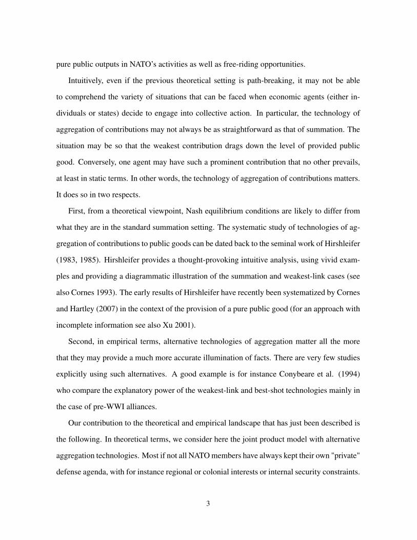
DEFi,t =αi +βGDPi,t +δ1BS1i,t−1 +δ2SUM2i,t−1 (20)

DEFi,t =αi +βGDPi,t +δ1SUM1i,t−1 +δ2BS2i,t−1 (21)

Both estimations identify two breakpoints in 1970 and 1990. Estimations of equation 20 yield

a model where BS1 and SUM2 are significant with a break in 1970 and another in 1990.

Estimations of equation 21 also provide a model where SUM1 and BS2 are significant, with

the same time break as with equation 20 (see tables 2 and 3). From those contradictory results,

technology shifts do appear in 1970 and 1950, but at this stage those shifts cannot be sorted

out.

11

Table 2. Estimation of time breaks for equation 20.

GDP BS1 SUM2 GDP BS1 SUM2Model 1955 0.475*** (dropped) 0.017 Model 1981 0.468*** 0.003 0.005Model 1956 0.480*** 0.001 0.001 Model 1982 0.485*** 0.001 0.001Model 1957 0.493*** 0.004 -0.000 Model 1983 0.487*** -0.001 -0.001Model 1958 0.470*** -0.006 -0.003 Model 1984 0.493*** 0.003 0.002Model 1959 0.491*** -0.002 -0.004 Model 1985 0.495*** 0.002 0.001Model 1960 0.457*** -0.003 0.002 Model 1986 0.497*** -0.005 -0.004Model 1961 0.446*** -0.003 0.003 Model 1987 0.513*** -0.004 -0.006Model 1962 0.485*** -0.004 -0.004 Model 1988 0.519*** -0.003 -0.005Model 1963 0.471*** -0.008 -0.006 Model 1989 0.518*** -0.006 -0.007Model 1964 0.484*** -0.004 -0.004 Model 1990 0.533*** -0.010* -0.013**Model 1965 0.472*** 0.009 0.010* Model 1991 0.537*** 0.001 -0.003Model 1966 0.461*** 0.005 0.008 Model 1992 0.547*** -0.005 -0.010*Model 1967 0.484*** -0.001 -0.001 Model 1993 0.547*** -0.007 -0.011*Model 1968 0.498*** -0.004 -0.006 Model 1994 0.555*** -0.004 -0.010*Model 1969 0.477*** -0.008 -0.007 Model 1995 0.538*** -0.007 -0.010*Model 1970 0.472*** -0.013** -0.011* Model 1996 0.533*** -0.003 -0.006Model 1971 0.472*** -0.005 -0.003 Model 1997 0.522*** -0.005 -0.006Model 1972 0.494*** -0.007 -0.008 Model 1998 0.517*** -0.002 -0.004Model 1973 0.457*** -0.006 -0.001 Model 1999 0.519*** 0.004 0.000Model 1974 0.459*** -0.009 -0.004 Model 2000 0.508*** 0.000 -0.001Model 1975 0.491*** -0.007 -0.008 Model 2001 0.518*** 0.012* 0.007Model 1976 0.475*** -0.001 -0.000 Model 2002 0.508*** 0.012* 0.008Model 1977 0.476*** -0.004 -0.003 Model 2003 0.505*** 0.007 0.005Model 1978 0.483*** -0.001 -0.001 Model 2004 0.502*** 0.004 0.002Model 1979 0.472*** 0.001 0.003 Model 2005 0.504*** -0.001 -0.003Model 1980 0.466*** 0.000 0.003 Model 2006 0.478*** -0.001 (dropped)(*), (**), (***): respectively significant at 10%, 5% and 1% level.

12

Table 3. Estimation of time breaks for equation 21.

GDP SUM1 BS2 GDP SUM1 BS2Model 1955 0.478*** (dropped) -0.001 Model 1981 0.470*** -0.006 -0.003Model 1956 0.481*** -0.001 -0.001 Model 1982 0.486*** -0.000 -0.001Model 1957 0.494*** 0.001 -0.003 Model 1983 0.487*** 0.001 0.001Model 1958 0.469*** 0.003 0.006 Model 1984 0.495*** -0.002 -0.003Model 1959 0.490*** 0.004 0.003 Model 1985 0.497*** -0.001 -0.002Model 1960 0.456*** -0.002 0.003 Model 1986 0.496*** 0.004 0.005Model 1961 0.446*** -0.004 0.002 Model 1987 0.512*** 0.006 0.004Model 1962 0.484*** 0.004 0.004 Model 1988 0.517*** 0.005 0.003Model 1963 0.469*** 0.006 0.008 Model 1989 0.514*** 0.007 0.006Model 1964 0.483*** 0.004 0.004 Model 1990 0.526*** 0.013** 0.010*Model 1965 0.476*** -0.010* -0.009 Model 1991 0.535*** 0.002 -0.002Model 1966 0.463*** -0.009 -0.006 Model 1992 0.541*** 0.009* 0.005Model 1967 0.484*** 0.001 0.001 Model 1993 0.540*** 0.010* 0.006Model 1968 0.497*** 0.006 0.004 Model 1994 0.549*** 0.009 0.003Model 1969 0.474*** 0.007 0.009 Model 1995 0.532*** 0.009 0.006Model 1970 0.467*** 0.011* 0.014** Model 1996 0.530*** 0.005 0.002Model 1971 0.470*** 0.004 0.006 Model 1997 0.519*** 0.006 0.005Model 1972 0.492*** 0.008 0.007 Model 1998 0.516*** 0.004 0.002Model 1973 0.455*** 0.002 0.007 Model 1999 0.519*** -0.000 -0.004Model 1974 0.457*** 0.004 0.009 Model 2000 0.508*** 0.001 0.000Model 1975 0.489*** 0.008 0.007 Model 2001 0.521*** -0.006 -0.012*Model 1976 0.475*** 0.000 0.001 Model 2002 0.511*** -0.007 -0.011*Model 1977 0.475*** 0.003 0.004 Model 2003 0.506*** -0.004 -0.006Model 1978 0.483*** 0.001 0.001 Model 2004 0.502*** -0.002 -0.004Model 1979 0.473*** -0.003 -0.001 Model 2005 0.503*** 0.003 0.001Model 1980 0.467*** -0.003 -0.000 Model 2006 0.475*** 0.017 (dropped)(*), (**), (***): respectively significant at 10%, 5% and 1% level.

13

There would be a three period model, 1955-1970, 1971-1990 and 1991-2006, with possi-

ble alternation of technologies. We keep those dates as breakup points for the next investiga-

tions.

The third step indeed will consider these fixed dates and will allow for technology changes

from one period to another. Breakpoints are extended accordingly:

SUM1i,t−1 =(date1970)(SUMi,t−1) (22)

SUM2i,t−1 =(date1990−date1970)(SUMi,t−1) (23)

SUM3i,t−1 =(1−date1990)(SUMi,t−1) (24)

BS1i,t−1 =(date1970)(BSi,t−1) (25)

BS2i,t−1 =(date1990−date1970)(BSi,t−1) (26)

BS3i,t−1 =(1−date1990)(BSi,t−1) (27)

SUM1, SUM2 and SUM3 correspond to the summation technology respectively before 1970,

from 1971 to 1990, and after 1990. The same periods of time and the best-shot variables are

denoted by BS1, BS2 and BS3. Consequently, the three periods and the two technologies bring

14

about eight different models providing all possible combinations of technologies over time.

Model 1 : DEFi,t = αi +βGDPi,t +δ1SUM1i,t−1 +δ2SUM2i,t−1 +δ3SUM3i,t−1

Model 2 : DEFi,t = αi +βGDPi,t +δ1SUM1i,t−1 +δ2SUM2i,t−1 +δ3BS3i,t−1

Model 3 : DEFi,t = αi +βGDPi,t +δ1SUM1i,t−1 +δ2BS2i,t−1 +δ3SUM3i,t−1

Model 4 : DEFi,t = αi +βGDPi,t +δ1SUM1i,t−1 +δ2BS2i,t−1 +δ3BS3i,t−1

Model 5 : DEFi,t = αi +βGDPi,t +δ1BS1i,t−1 +δ2SUM2i,t−1 +δ3SUM3i,t−1

Model 6 : DEFi,t = αi +βGDPi,t +δ1BS1i,t−1 +δ2SUM2i,t−1 +δ3BS3i,t−1

Model 7 : DEFi,t = αi +βGDPi,t +δ1BS1i,t−1 +δ2BS2i,t−1 +δ3SUM3i,t−1

Model 8 : DEFi,t = αi +βGDPi,t +δ1BS1i,t−1 +δ2BS2i,t−1 +δ3BS3i,t−1

Table 4 gives the estimation results of models 1 to 8 using fixed effects OLS with PCSE.

Only the estimates of models 2, 4, 5 and 7 are all significant. The competing models are

systematically evaluated against the seven others by running J tests. The results are given in

tables 6 to 13 (see appendix). The last row of column labeled “test a−b” reports the coefficient

of the J test. If this coefficient is significant, model b is better than model a. Table 5 sum-

marizes these results. “Yes” means that the model in row significantly dominates the model

in column while “No” means that model in row does not significantly dominate the model in

column. As suggested by table 5, none of the seven other models are better than model 5 and

model 5 always beats the other models except for model 4. According to these results, we

may conclude that NATO’s strategy is thus first characterized by a best-shot situation from

1955 to 1970; from this date onwards, a summation technology prevails with an increase in

strategic behavior after 1990 (see Table 4). We now move on to a more detailed presentation

and discussion of the evolution of NATO’s strategy.

15

Table 4. Estimation results of models 1 to 8 using fixed effects OLS with PCSE

Variable Model 1 Model 2 Model 3 Model 4 Model 5 Model 6 Model 7 Model 8GDP 0.540*** 0.527*** 0.532*** 0.516*** 0.538*** 0.506*** 0.523*** 0.507***SUM1 -0.010 -0.011* 0.001 0.013**SUM2 -0.009 -0.013* -0.013*** 0.000SUM3 -0.013 -0.002 -0.017*** -0.013***BS1 -0.016*** -0.003 -0.012* 0.000BS2 0.003 0.016** -0.010* 0.003BS3 0.010* 0.013* -0.002 0.000

R2 0.979 0.978 0.978 0.977 0.979 0.976 0.978 0.976(*), (**), (***): respectively significant at 10%, 5% and 1% level.

Table 5. Estimation results of the J tests

Variable Model 1 Model 2 Model 3 Model 4 Model 5 Model 6 Model 7 Model 8Model 1 . Yes No Yes No Yes Yes NoModel 2 Yes . Yes Yes No Yes No YesModel 3 No Yes . Yes No Yes Yes YesModel 4 Yes Yes Yes . No Yes Yes YesModel 5 Yes Yes Yes No . Yes Yes YesModel 6 No Yes No Yes No . No NoModel 7 Yes No Yes Yes No Yes . YesModel 8 No Yes Yes No No No No ."Yes" means that model in row significantly dominates model in column.

16

4. Discussion and conclusion

In this study, we have used the now standard interpretation of NATO’s strategies as the pro-

vision of joint defense products (Sandler and Hartley 2001). In the field of defense, multiple

outputs whose publicness varies are involved, including local public goods (e.g., national in-

terests’ defense programs). Those ally-specific benefits are mainly derived from conventional

forces and they yield no benefits to the other allies. However, conventional forces can also

be deployed within the alliance, for instance in an effort to protect common exposed borders.

Then, they are susceptible to force thinning. They can also be projected in joint peace-keeping

operations, in which case a congestion effect may occur, when projection capabilities are over-

stretched by participation in too many such operations. Conventional forces when used in an

alliance thus provide impurely public alliance-wide benefits.

Although NATO does use conventional forces, it is not a "conventional" alliance. Af-

ter WWII, the Soviet Union is expanding westwards via satellite states. It also keeps run-

ning a heavy defense industry at a wartime pace. European democracies are rebuilding their

economies while the United States largely converts defense industries to civil applications and

markets. Western countries, which are not yet formal allies, thus face the expansionism of a

Soviet Union which has acquired a conventional weapons advantage. The so-called Truman

doctrine (after the declaration of March 1947) rests on the fact that the United States possesses

the nuclear weapon whereas the Soviet Union does not. In this context, NATO is created in

April 1949. Mutual assistance is formalized under Article 5 of the Treaty: "The Parties agree

that an armed attack against one or more of them in Europe or North America shall be con-

sidered an attack against them all and consequently they agree that, if such an armed attack

occurs, each of them, in exercise of the right of individual or collective self-defence recog-

nised by Article 51 of the Charter of the United Nations, will assist the Party or Parties so

attacked by taking forthwith, individually and in concert with the other Parties, such action as

17

it deems necessary, including the use of armed force, to restore and maintain the security of

the North Atlantic area."

The United States provides nuclear deterrence to its allies but its monopoly on nuclear

weapons only lasts until August 1949! However, the nuclear effort of the western alliance

is such that NATO soon has a first-strike advantage (through a pre-emptive strike aimed at

neutralizing Soviet nuclear assets). Article 5 of the Treaty is complemented by the directives

MC3 of October and November 1949 which explicitly mention nuclear strikes. Directive

MC48 of November 1954 defines nuclear deterrence as a purely public alliance-wide benefit

(Directives MC48/1 of November 1955 and MC48/2 of May 1957 describe more precisely the

implementation patterns). NATO is thus an "unconventional" alliance set up in the emerging

nuclear era. Doctrines and strategies will of course evolve afterwards, giving more or less

weight to strategic and conventional weapons. Nevertheless, the joint product framework will

remain and this "impurity of defense," as labeled by Sandler (1977) will adequately depict the

strategic landscape of post WWII western security policy.

We have tried to contribute to another dimension of the debate on Nato, namely the way

in which contributions of allies to their international organization articulate themselves in a

"social composition function" to use the words of Hirshleifer. Broadly depicted, three such

functions can be used when analyzing an alliance. A straightforward aggregation process is

the summation of all the allies’ efforts (for instance by adding troops or armored divisions to

the joint forces). A quite different situation occurs when an alliance has to rely on the minimal

contribution to ensure collective protection. In that case, aggregation follows a weakest-link

technology. A third aggregator is the so-called best-shot, whereby the largest of the individual

contributions determines the collective defense output.

Our intuition was that in the case of NATO, the summation and best-shot aggregators could

be relevant but that we would have to find out the pertinent periodization. A single technology

would not necessarily be relevant throughout our long period of study of NATO (1955-2006).

18

To investigate that, we have modeled allies’ defense expenditures as a function of their GDP

and of the aggregation technology.

It is always tempting to accumulate independent variables in the econometric regression

in order to capture as many influences as possible. Though it cannot be contended that GDP

summarizes them all, it may adequately synthesize the fiscal constraints faced by the allies

over those decades of cooperation. As was expected, the contribution of an ally logically de-

pends on the country’s own GDP. We estimate that over the period 1955-2006, a 10% variation

in country i’s GDP would lead to a 5.38% variation of the same sign in its contribution to the

alliance expenditures (see Model 5 of Table 4). Military budgets do depend on the ability of

nations to produce wealth and they obviously are not disconnected from economic activity.

As to the core of our study, namely the nature and influence of the aggregation technology

of contributions, we have allowed an unknown number of dates for technology shifts over the

study period. Two breakpoints emerged, one in 1970, the other in 1990. These breakpoints

thus delineate three periods characterized by different composition functions.

From 1955 to 1970, NATO’s strategy relies mostly on the US military expenditures. More

precisely, it rests on US nuclear deterrence as a credible commitment. We have previously

mentioned that the United States has a first-strike advantage. It soon develops a second strike

capability (its stockpile of nuclear weapons is sufficient to do so). In this context, we demon-

strate that the best-shot technology of aggregation is predominant. Deterrence is mostly a

pure public good. Since its benefits are largely non-excludable, one can expect opportunistic

behavior on the part of the non best-shot allies. There would thus be a negative relationship

between their defense outlays and those of the best-shot. Our estimates indeed show that a

10% increase in the US defense expenditures yields a 0.16% decrease in the defense expendi-

tures of the other members of the alliance (see Model 5 of Table 4).

More surprising is perhaps the 1970 breakpoint since the institutional break is 1967. Our

estimations illuminate the lag between the doctrinal decision and its actual implementation.

19

The doctrine of flexible response, or flexible escalation as it is sometimes and more ade-

quately labeled, does receive political approval in May 1967 (DPC/D (67)23: Decisions of

the Defence Planning Committee in Ministerial Session). This leads to directive MC14/3: its

final version is issued in January 1968. Furthermore, this directive is complemented with a

companion document, directive MC48/3 ("Measures to Implement the Strategic Concept for

the Defence of the NATO Area"). As is made clear in its title, this directive aims at giving

practical effect to directive MC14/3. Directive MC48/3 is issued in its final form in December

1969. It will shape NATO’s strategy until the end of the Cold War.

From 1970 until 1990, NATO’s strategy is that of the flexible response or escalation doc-

trine. It is adequate since the Soviet Union has intensified its production of nuclear weapons,

thus lessening NATO’s strategic advantage. Non-nuclear engagements are to be the first re-

sponse to an aggression. Conventional forces should be used on the primary front or employed

for the opening of a new ground front (or at sea). Afterwards, nuclear weapons can succes-

sively be used demonstratively, then selectively on interdiction targets. The general nuclear

response is conceived as the ultimate deterrent only. In this renewed context, the comple-

mentarity between strategic and conventional forces is much bigger than during the previous

period. This is really an era of joint defense products which requires and induces a greater

involvement of the allies. Nuclear weapons can even have a quasi tactical employment on a

conventional front, making them an element of the strategy rather than the strategy itself.

In this renewed context, one can expect that the technology of aggregation of contribution

will move from best-shot to summation and this is what our results support. Strategic, tactical

and conventional weapons are mixed and they become complementary in the overall strategy.

The ensuing increased implication of allies should lessen opportunistic behaviors insofar as

the share of non-excludable purely public benefits decreases. Since the participation of each

member to the alliance now matters, free-riding could then be less pronounced than in the

best-shot case, as indicated by Hirshleifer (1983). Our econometric results show that a 10%

20

increase in the defense expenditures of alliance members j 6=i would lead to a 0.13% drop in the

participation of country i to NATO’s expenditures. NATO members still evince opportunistic

behavior, however to a lesser extent than within a best-shot framework.

From 1991 until 2006, NATO’s strategy dramatically changes as the international arena

also dramatically moves to a post Cold War world. The new security challenges arise from

nationalist or territorial disputes, resource claims, ethnic and religious conflicts. NATO’s

Heads of State and Government meet in July 1990 and they agree on the need to radically

review their strategy. This leads to the Alliance’s Strategic Concept of 1991. The next version

of April 1999 confirms the initial one and provides inflexions with regard to the evolving

international situation. The Comprehensive Political Guidance of November 2006 comes of

course too late in our sample to have any effect.

The post Cold War security environment calls for a new strategy, usually labeled the crisis-

management doctrine. NATO settles to the task of peacekeeping and peace enforcement. It

contributes to regional or even world stability and security, which benefits both contributors

and non-contributors. Beside this non excludable output, country-specific outputs take the

form of post-conflict reconstruction and rebuilding contracts, assurances of more stability for

countries in closer proximity to the conflict or with trade interests in the region. Nevertheless,

there is plausibly a greater share of non excludable collective benefits associated with the

alliance’s new strategic concept.

Concurrently, the implementation of the new strategy rests on mobile forces drawn from

multiple allies and deployed at great cost (from under $300 million in 1988 to over an annual

$300 billion in the mid-1990s; Sandler and Hartley 1999). This increased tactical integration

takes place in a context of dramatic declines in resources allocated to defense, due to the

downsizing of forces. The collective outcome is thus subject to crowding effects. Rapid

deployment forces are soon congested: the number of missions to cope with is such that the

overstretching of capacities is a concrete threat. This is all the more so the case that the burden

21

is mostly shouldered by the United States, France, Great Britain and Germany. Disproportion

of efforts between the latter contributors and the others probably grows, amplified by the fact

that projection capabilities require initial and sustained investment so that allies that do not

invest in the first place cannot do it at short notice in case of a crisis.

On the whole, the summation technology remains the aggregator as confirmed by our

estimations. Conventional forces are on the frontline, and the strategic nuclear forces stay

behind. Sections 62 to 64 of the 1999 Alliance’s Strategic Concept state it clearly. The nuclear

forces of the United States, France and Great Britain keep to their mission of deterrence: they

are there to "demonstrate that aggression of any kind is not a rational option" (Section 62).

The strategic context of the 1990s and after is such that there is probably an increased share

of pure public inputs in NATO’s activities. This is partly mitigated by the regional dimension

of some conflicts (think of the Balkans) or of the economic stakes of others (think of Kuwait)

which would dampen potential opportunism. One could thus expect increased opportunistic

behaviors, but not necessarily a large augmentation. Our estimates for the last period of our

study of the alliance show that a 10% increase in the defense expenditures of countries j 6=i

would yield a 0.17% decrease in country i’s military expenditures. Compared with the 0.13%

drop of the previous period, free riding increases (see Model 5 of Table ).

To sum up, our panel data analysis of NATO over the period 1955-2006 evidences ag-

gregation technology breakpoints in 1970 and 1990. We show that NATO follows a best-shot

aggregator for 1955-1970 and summation for 1971-1990 as well as for 1991-2005. Free riding

is always present. It decreases from the first to the second period as the share of pure public

outputs of collective defense activities diminishes. Purely public benefits are more present

during the third period, giving more room to opportunistic behaviors.

Embracing such a long time period and aiming to assess the huge endeavor of NATO obvi-

ously implies that our study has limits. We shall now try to point out a few of them. First, the

evolution of the political context is not taken into account. Allies face internal pressures from

22

their public opinions, their ideological inclinations vary through time and space. The fiscal

constraint also evolves, with for instance a global increase in social security expenditures. As

a further research step, one could envisage adding for instance dummy variables for left-wing

or right-wing national policies, for countries with strong communist parties, etc. This would

enrich the analysis, probably at the cost of less clarity with respect to our initial aim, which is

more the assessment of aggregation technology change than behavioral analysis.

In a way, this last remark leads us to another limit of our analysis. We have not really clar-

ified, if ever it is possible within our framework, why the alliance did switch from best-shot

to summation composition functions. Was it more a matter of technology of conflict than of

deliberate doctrinal choice? A partial answer lies in the consequences of the Cuban missile

crisis. Initially set as a chicken game where the Soviet concedes but where the United States

does not implement its threat of massive nuclear strike, the game is thus played cooperatively

which helps avoid direct confrontation. The USSR then intensifies its production of strate-

gic and tactical nuclear weapons, thus lessening NATO’s strategic advantage represented by

the US best-shot. The flexible response doctrine provides answers to acts of aggression that

are commensurate to the actual threat. Conventional, tactical and strategic weapons become

complementary. However, this remains to be further investigated, the two dimensions, tech-

nological and behavioral, remaining somewhat entangled in our study.

The previous interrogation brings in another one. If a shift in the composition function

is identified, whether driven by technology or by deliberate choice, to what extent does it

matter? Apart from the industrial and military consequences of the shift, we have shown that

it has a significant impact on the opportunistic behaviors of the allies. In this respect, the

aggregation technology matters. Once in place, the social composition of the alliance shapes

the behavioral framework of the allies, for instance their choice between the supranational and

the local defense public goods.

23

Acknowledgments

Earlier versions have been presented at the European Public Choice Society meetings in Izmir, Turkey, in April

2010 and at the Pearl seminar at the University of Eastern Piedmont, Italy, in May 2010. We have received helpful

comments by Professor COL Atin Basuchoudhary from the Virginia Military Institute and by Doctor Emanuele

Canegrati from the Italian Parliamentary economic advisers committee. Finally, comments by two anonymous

reviewers and by the editor have contributed to substantially enhance the first versions of the manuscript. Sole

responsibility for any remaining shortcomings rests with the authors.

Appendix

Table 6. J tests : Model 1 against the other models

test1_1 test1_2 test1_3 test1_4 test1_5 test1_6 test1_7 test1_8GDP 0.000 0.001 -0.018 0.072 -0.027 -0.274 -0.158 -0.098SUM1 0.000 -0.018 -0.009 -0.010 0.025 -0.003 0.019 -0.008SUM2 0.000 -0.018 -0.010 -0.010 0.025 -0.006 0.017 -0.010SUM3 0.000 -0.019 -0.010 -0.012 0.025 -0.006 0.018 -0.011J test coefficients 1.000*** 1.019* 1.049 0.899** 1.042*** 1.606 1.326** 1.258

(***), (**), (*) respectively significant at 1%, 5%, 10%


test2_1 test2_2 test2_3 test2_4 test2_5 test2_6 test2_7 test2_8GDP -0.239 0.000 -2.352** 0.049 0.035 -2.585** -1.130 -2.067*SUM1 0.009 0.000 0.0116* 0.011* 0.008 0.024*** -0.021 0.023***SUM2 0.008 0.000 0.004 0.012** 0.008 0.010* -0.028 0.012**BS3 0.0107* 0.000 0.023*** 0.011* 0.009 0.022*** -0.022 0.022***J test coefficients 1.439 1.000*** 5.413** 0.922** 0.927** 6.153*** 3.216 5.111**

(***), (**), (*), respectively significant at 1%, 5%, 10%

24


test3_1 test3_2 test3_3 test3_4 test3_5 test3_6 test3_7 test3_8GDP -0.068 -0.630 0.000 -0.393 -0.216 -18.809 -0.438 -49.698***SUM1 0.003 0.015** 0.000 -0.011* -0.007 0.021 0.0125** 0.011*SUM3 0.003 0.018** 0.000 -0.012** -0.006 0.008 0.012* -0.011**BS2 0.003 0.015** 0.000 -0.014* -0.008 -0.088 0.010** -0.275***J test coefficients 1.125 2.182*** 1.000*** 1.787*** 1.406*** 38.255 1.861*** 99.024***



test4_1 test4_2 test4_3 test4_4 test4_5 test4_6 test4_7 test4_8GDP -0.905 0.069 -3.803* 0.000 -0.585 -13.090 0.045 48.548SUM1 0.017*** 0.013** 0.006 0.000 -0.015 0.024*** 0.012** 0.013**BS2 0.015** 0.015** -0.008 0.000 -0.018 -0.051 0.013** 0.293BS3 0.023*** 0.014** 0.024*** 0.000 -0.013 0.015** 0.012* 0.035J test coefficients 2.666** 0.865** 8.141** 1.000*** 2.107 26.939* 0.935** -94.698



test5_1 test5_2 test5_3 test5_4 test5_5 test5_6 test5_7 test5_8GDP 1.869 0.097 2.127* 1.135 0.000 2.444* 0.103 2.115*SUM2 -0.010 -0.014** -0.014** -0.028 0.000 -0.011* -0.012** -0.012**SUM3 -0.025 -0.015** -0.031*** -0.035 0.000 -0.024*** -0.013* -0.024***BS1 -0.017*** -0.015*** -0.023*** -0.034 0.000 -0.025*** -0.013** -0.024***J test coefficients -2.469 0.831 -2.982 -1.135 1.000*** -3.766 0.835 -3.105



test6_1 test6_2 test6_3 test6_4 test6_5 test6_6 test6_7 test6_8GDP -3.144* -0.572* -4.862*** -0.355 -0.205 0.000 -0.422 0.085SUM2 -0.020* -0.016** -0.004 0.011* 0.006 0.000 -0.012** 0.000BS1 -0.011* -0.015*** 0.013* 0.013* 0.007 0.000 -0.010* 0.000BS3 0.006 -0.013** 0.036*** 0.013* 0.009 0.000 -0.010* 0.000J test coefficients 6.842** 2.088*** 10.121*** 1.691*** 1.378*** 1.000*** 1.845*** 0.834


25


test7_1 test7_2 test7_3 test7_4 test7_5 test7_6 test7_7 test7_8GDP 4.064* 1.635 -7.868** 0.052 0.050 11.889 0.000 -4.156SUM3 -0.041** -0.041 0.011 -0.012** -0.008 -0.021*** 0.000 -0.013**BS1 -0.024*** -0.037 -0.024*** -0.012* -0.009 -0.027** 0.000 -0.011BS2 -0.010* -0.031 -0.052*** -0.012* -0.008 0.041 0.000 -0.035J test coefficients -6.565* -2.062 15.793** 0.929** 0.909** -22.461 1.000*** 9.232



test8_1 test8_2 test8_3 test8_4 test8_5 test8_6 test8_7 test8_8GDP -0.408 0.062 -4.906*** -0.020 -0.089 0.024 -0.011 0.000BS1 0.011 -0.013 -0.021 -0.020 0.005 0.003 0.006 0.000BS2 0.011 -0.012 -0.039 -0.020 0.005 0.003 0.006 0.000BS3 0.015 -0.012 0.001 -0.020 0.006 0.003 0.005 0.000J test coefficients 1.709 0.869* 10.234*** 1.058** 1.162*** 0.955 1.026** 1.000***


References

Beck, N. and Katz, J. (1995). What to do (and not to do) with time series cross-section data.American Political Science Review, 89:634–647.

Bergstrom, T. C., Blume, L., and Varian, H. (1986). On the private provision of public goods.Journal of Public Economics, 29:25–49.

Conybeare, J., Murdoch, J., and Sandler, T. (1994). Alternative collective-goods models ofmilitary tactics. Economic Inquiry, 32:525–542.

Conybeare, J. A. and Sandler, T. (1990). The Triple Entente and the Triple Alliance 1880-1914: A collective goods approach. The American Political Science Review, 84:1197–1206.

Cornes, R. (1993). Dyke maintenance and other stories: Some neglected types of publicgoods. The Quarterly Journal of Economics, 91:25–49.

Cornes, R. and Hartley, K. (2007). Weak links, good shots and other public goods games:building on BBV. Journal of Public Economics, 108:1684–1707.

Cornes, R. and Sandler, T. (1984). Easy riders, joint production and public goods. TheEconomic Journal, 94:580–598.

Cornes, R. and Sandler, T. (1996). The theory of externalities, public goods and club goods.Cambridge University Press.

Gadea, M., Pardos, E., and Perez-Fornies, C. (2004). A long-run analysis of defence spendingin the NATO countries (1960-99). Defence and Peace Economics, 15:231–249.

26

Hansen, L., Murdoch, J. C., and Sandler, T. (1990). On distinguishing the behavior of nuclearand non-nuclear allies in NATO. Defence Economics, 1:37–55.

Hirshleifer, J. (1983). From weakest-link to best-shot: The voluntary provision of publicgoods. Public Choice, 41:371–386.

Hirshleifer, J. (1985). From weakest-link to best-shot: Correction. Public Choice, 46:221–223.

Khanna, J. and Sandler, T. (1996). Nato burden sharing: 1960-1992. Defence and PeaceEconomics, 7:115–133.

Murdoch, J. C. and Sandler, T. (1984). Complementarity, free riding, and the military expen-ditures of NATO allies. Journal of Public Economics, 25:83–101.

Olson, M. and Zeckhauser, R. (1966). An economic theory of alliances. Review of Economicsand Statistics, 48:266–279.

Oneal, J. R. and Elrod, M. (1989). NATO burden sharing and the forces of change. Interna-tional Studies Quarterly, 33:435–456.

Pesaran, H. (2003). A simple panel unit root test in the presence of cross section dependence.Working paper, University of Southern California.

Samuelson, P. A. (1954). The pure theory of public expenditure. Review of Economics andStatistics, 36:387–389.

Samuelson, P. A. (1955). Diagrammatic exposition of a theory of public expenditure. Reviewof Economics and Statistics, 37:350–357.

Sandler, T. (1977). Impurity of defense: An application to the economics of alliances. Kyklos,30:433–460.

Sandler, T. (2006). Regional public goods and international organizations. Review of Interna-tional Organizations, 1:5–25.

Sandler, T. and Forbes, J. F. (1980). Burden sharing, strategy, and the design of NATO.Economic Inquiry, 18:425–444.

Sandler, T. and Hartley, K. (1999). The political economy of NATO: Past, present, and intothe 21st century. Cambridge.

Sandler, T. and Hartley, K. (2001). Economics of alliances: The lessons for collective action.Journal of Economic Literature, 39:869–896.

Sandler, T. and Murdoch, J. (2000). On sharing NATO defence burdens in the 1990’s andbeyond. Fiscal Studies, 21:297–327.

27

Smith, R. P. (1989). Models of military expenditure. Journal of Applied Econometrics, 4:345–359.

Warr, P. (1983). The private provision of a public good is independent of the distribution ofincome. Economics Letters, 17:207–211.

Wooldridge, J. M. (2002). Econometric analysis of cross section and panel data. CambridgeMA, MIT Press.

Xu, X. (2001). Group size and the private supply of a best-shot public good. European Journalof Political Economy, 17:897–904.

28

Documents

The role of aggregation technologies in the provision of