The role of attitudes in determining individual behavior ... · Prof. Rico Maggi, supervisor ... Structure of the questionnaire: ... Data were collected through a survey conducted

The role of attitudes in determining individual behavior in transportation - from

psychology to discrete choice modeling

A dissertation presented by

Antonio Borriello

Submitted to the

Faculty of Economics

Università della Svizzera Italiana

For the degree of

Ph.D. in Economics

Thesis Committee:

Prof. Rico Maggi, supervisor, Università della Svizzera italiana

Prof. Massimo Filippini, internal examiner, Università della Svizzera italiana

Prof. Kay Axhausen, external examiner, ETH Zürich

January 2017

2

“If we knew what it was we were doing, it would not be called research, would it?”

Albert Einstein

3

Contents

Introduction ..............................................................................................................................................................5

References ............................................................................................................................................................. 12

Chapter 1. Exploiting Evaluative Space Grids to stochastically measure ambivalence/indifference .................... 14

Abstract ............................................................................................................................................................. 14

1.1. Introduction .......................................................................................................................................... 15

1.2. Ambivalence and indifference measures ............................................................................................. 19

1.3. Methodology ......................................................................................................................................... 24

1.3.1. Tobit Model: Indirect (scores) approach ........................................................................................ 24

1.3.2. Ordered Logit model approach: Direct (observed ratings) approach ............................................ 25

1.4. Empirical data ....................................................................................................................................... 29

1.5. Estimation sample results .................................................................................................................... 31



1.6. Out of sample results ............................................................................................................................ 37



1.7. Discussion and conclusions .................................................................................................................. 39

References ......................................................................................................................................................... 42

Chapter 2. The implementation of the Evaluative Space Grid in a hybrid choice model to overcome the

disadvantages of measuring attitudes using common scales. .............................................................................. 45

Abstract ............................................................................................................................................................. 45

2.1. Introduction .......................................................................................................................................... 46

2.2. Evaluative Space Grid (ESG) .................................................................................................................. 49

2.3. Methodology ......................................................................................................................................... 50

2.4. Empirical data ....................................................................................................................................... 54

2.4.1. Sample composition ....................................................................................................................... 54

2.4.2. Structure of the questionnaire: SP experiment .............................................................................. 55

2.4.3. Structure of the questionnaire: attitudinal questions ................................................................... 57

2.5. The model.............................................................................................................................................. 58

2.6. Results ................................................................................................................................................... 62

2.6.1. Structural model ............................................................................................................................ 62

2.6.2. Measurement model ..................................................................................................................... 63

4

2.6.3. Discrete choice model .................................................................................................................... 66

2.6.4. Effect of latent variables ................................................................................................................ 68

2.7. Discussion and conclusions .................................................................................................................. 71

References ......................................................................................................................................................... 74

Chapter 3. Generalized versus localized attitudinal responses in discrete choice ................................................ 77

Abstract ................................................................................................................................................................. 77

3.1. Introduction .......................................................................................................................................... 78

3.2. Theoretical background ........................................................................................................................ 81

3.3. Case study ............................................................................................................................................. 82

3.3.1. The survey ...................................................................................................................................... 82

3.3.2. The evaluative space grid (ESG) ..................................................................................................... 85

3.3.3. Sample composition ....................................................................................................................... 86

3.4. Model .................................................................................................................................................... 87

3.5. Results ................................................................................................................................................... 89

3.5.1. Localized attitudes ......................................................................................................................... 91

3.5.2. Structural equation model ............................................................................................................. 94

3.5.3. Choice model ................................................................................................................................. 98

3.5.4. Discussing the different models ................................................................................................... 100

3.6. Conclusions ......................................................................................................................................... 101

References ....................................................................................................................................................... 104

Conclusion ........................................................................................................................................................... 107

5

Introduction

This dissertation is the outcome of a PhD program in Economics focused on modelling individual

preferences in the context of transportation. Its ambition is to improve the understanding of individual

choices using discrete choice model techniques (HDCM). The framework of HDCM consists of the

simultaneous estimation of two processes, a structural equation model and a choice model. Whilst the

former explores the composition of the psychological factors, the latter predicts individual choices

among a set of discrete alternatives. This methodology was proposed by McFadden (1986) in response

to the critiques of behavioral economics regarding the acceptance of individual rationality in the

context of choice behavior. Indeed, behavioral economists disagree with the bounded rationality of

economic agents and suggested a wider theoretical framework according to which psychological, social,

cognitive, and emotional factors play a notable role in determining economic decisions of individuals

(Kahneman et al., 1991; Kahneman and Ritov, 1994; Kahneman et al., 1999; Thaler, 1980 and 1985). In

accordance with this theoretical framework, McFadden states that “the theory of the economically

rational utility-maximizing consumer, interpreted broadly to admit the effects of perception, state of

mind, and imperfect discrimination, provides a plausible, logically unified foundation for the

development of models of various aspects of market behavior” (p. S14, 1980). Hybrid discrete choice

model represents a technique able to incorporate the irregularities and idiosyncratic features of choice

behavior, due to perceptions, attitudes information processing, context and cognitive processes, into

the systematic and invariant features typical of the random utility model (Ben-Akiva et al., 2002). Within

this framework, the random utility model (RUM) assumes that the characteristics of the decision-maker

and the attributes of the alternatives affect the decision process leading to the revealed choice. The

RUM is enhanced with several extensions, such as the inclusion of flexible disturbances, a latent

segmentation of the population or of latent psychological factors, which reduce the error computed in

modeling individual preferences.

In this setting, this dissertation aims at refining the way psychological factors are explored and framed

in the context of hybrid discrete choice model and includes three original articles, which are presented

as separate chapters. In any article, a methodological section, containing the innovation of the

econometrics steps, is followed by empirical work, based on datasets collected in the context of

transportation. Nevertheless, it is important to stress that the methodology described in this thesis can

6

be applied to any context. The first two chapters elucidate the advantages of using the Evaluative Space

Grid (ESG; Larsen et al., 2009), which is an instrument to measure attitudinal indicators, in the

framework of HDCM. Since the introduction of this methodology, numerous adaptations of the

econometric framework have been proposed in order to make the model more suitable for specific

cases (among others, mixed models, latent class models, multiple discrete-continuous models).

However, whilst the choice model part has evolved, the methodology employed for exploring the

psychological factors remained mostly unchanged. The rigidity of the structural equation model clashes

with the innovative and remarkable findings concerning the psychological aspects leading to the choice.

In order to reduce this “gap”, the first two chapters of this dissertation attempt to improve the way

psychological aspects are explored and are connected to the choice model in the framework of HDCM.

Data were collected through a survey conducted in the context of a Swiss National Science Foundation

project, namely PostCar World. Respondents, from three different linguistic regions of Switzerland,

completed a stated preference experiment on mode choice for commuting purpose and stated their

attitudes towards the pleasure of driving and environmental inclination, using the Evaluative Space Grid

instrument.

A notable concern discussed in psychology related to the measurement of psychological factors, which

may also affect the modeling of individual preferences, regards the distinction of individuals having an

ambivalent or indifferent attitude. Indeed, common response measures for evaluating attitudes,

emotions and affect, such as Likert and semantic differential scales, are unable to distinguish these two

categories of individuals. Indifference implies that a subject has no interest in the stimuli being studied,

being truly neutral in their attitude, reflected by low positive and negative reactions towards the object

under evaluation. Ambivalence, on the other hand, suggests that the subject experiences both positive

and negative valence towards the stimuli. When measured using traditional attitudinal scales, both

attitudes will likely result in the subject choosing the neutral option of the scale (Kaplan, 1972;

Thompson et al., 1995). To overcome this issue, Larsen et al. proposed using the Evaluative Space Grid,

which is a single-item measure of positivity and negativity. This instrument follows the theoretical

model proposed by Cacioppo and Berntson (1994), namely the Evaluative Space Model, who

demonstrate that both positive and negative feelings towards an object act as two distinct systems,

allowing for the independent and simultaneous assessment of positive/negative attitudes towards an

object. According to this theory, an increase in positive (negative) feelings is not necessarily connected

7

to a decrease of negative (positive) feelings. This finding has resulted in the literature distinguishing

between the concepts of ambivalence and indifference.

In several papers, ambivalence and indifference have been measured mainly by means of deterministic

indices (Kaplan, 1972; Thompson et al., 1995), which fail to recognize that recorded answers are the

result of underlying psychological latent constructs, and hence are imprecise expressions of an

individual's true attitude towards an object. Assuming attitudes are latent constructs, and hence not

directly measurable, the use of scores seems anachronistic. In this chapter, we suggest two different

approaches to model attitudes collected by means of ESGs according to their latent nature.

The first approach follows the scoring scheme proposed by Audrezet et al.’s (2016), who calculate a

(censored) deterministic score based on the individual response. We propose modelling this score by

means of a Tobit model, in which the latent dependent variable is predicted via socio-demographic

variables. It is worth noting that the model accounts for censoring of the dependent variable, consistent

with the bounds imposed when generating attitudinal scores using the approach proposed by Audrezet

et al..

In the second approach, using the observed attitudinal data captured using the ESG response

mechanism, we demonstrate how attitudinal data can be analyzed using a system of ordered logit

models. Also these models respect the assumption that the observed outcome obtained from the

response mechanism used is based on a latent construct. Such latent variable is decomposed into two

parts, a modelled component, and an unobserved error term which is randomly distributed over the

population of interest. The model produces not only an estimate of the value of the latent variable

based on the observed or modelled component used to explain the latent variable, but more

importantly, the stochastic nature of the error term translates into a probabilistic prediction of the

response outcome. By simultaneously estimating independent ordered logit models for the positive

and negative domains of the ESG, the approach allows for separate latent processes to explain

probabilistically the positive and negative domains of attitudes. Nevertheless, it is also possible to

determine to what degree the two processes are related by accounting for the correlation. Finally, by

placing restrictions on the parameter estimates derived from the various models, it is also possible to

test to what degree different latent processes exist across the positive and negative attitudinal

domains. It is our argument that for many applied fields, such as social behavior, political behavior and

8

marketing, the distinction between individuals having an ambivalent or indifferent attitude is of primary

importance and can add efficacy and efficiency to policies.

The second chapter of this dissertation illustrates the econometric steps to include the ESG in the

framework of a hybrid discrete choice model. The rationale of this work stems from the inaccurate

measurement of attitudes, which is common practice when modelling individual choices in

transportation. From an econometric point of view, an attitude is a variable that cannot be directly

measured (latent) but that can be defined through some indicators (or observable variables, items) net

of an error. The first problem concerns the number of indicators used to define the attitude itself:

because of their latent nature, the higher the number of observable variables suitable to measure the

attitude, the lower the error computed in the measuring process will be. Therefore, the omission of

relevant observable variables in defining an attitude increases the randomness of the latent variable

and, as a consequence, reduce its efficacy. A second problem is the misspecification of the attitude

itself. In many studies, choice modelers use a “direct measure” of what actually is a latent construct

(e.g. the latent variable comfort, which should be measured by means of observable indicators,

becomes a categorical attribute in the choice model) generating high aggregation of content. A poor

discrimination of content is also caused by the positioning of the items, used for measuring attitudes,

along the latent continuum. Otherwise stated, whilst psychologists include items with a positive,

neutral and negative valence covering the entire latent continuum domain when exploring an attitude

(i.e. they use appropriate wording aimed at capturing a possible positive, neutral and negative outcome

of the attitude), choice modelers usually use only items with an extreme positive or a negative valence.

A consequence of the lower discrimination and information is the aggregation of individuals with an

indifferent or ambivalent attitude in choice modeling applications when a common response

mechanism (e.g. Likert scale) is used. Indeed, as explained in the first chapter of this thesis, these two

categories of respondents select the central values of the scale, making the segmentation unfeasible.

To this aim, we propose using the Evaluative Space Grid, rather than a Likert scale to collect attitudinal

variables. This tool is able to disentangle individuals with an indifferent and an ambivalent attitude, as

well as those with a positive and a negative inclination. This chapter has a twofold ambition. From a

theoretical perspective, it integrates the ESG in the framework of discrete choice modelling: the grids

are modelled, in the structural equations, by means of two latent variables, representing positive and

negative domains respectively, whilst, in the measurement equations, two ordered logit regressions

9

link the observables items to the latent variables. The hybrid choice model does not include any specific

parameters to measure a direct effect of indifference and ambivalence on the alternatives. Rather,

probabilities of revealing an ambivalent or indifferent attitude are foreseen using the results of the

structural equation model. In addition to the methodological contribution, this work tests the

hypothesis that individuals with ambivalent and indifferent attitudes have different preferences in a

context of transportation mode choice for commuting trips and therefore the distinction of such

categories becomes of primary importance for making policies more effective. In particular, we show

that subjects who consider commuting by private car comfortable/handy and

uncomfortable/challenging at the same time (individuals revealing ambivalence) reveal different

preferences from those who judge commuting by private car neither comfortable/handy nor

uncomfortable/challenging (individuals having indifferent attitude), for 7 out of 8 alternatives of

transport. Furthermore, respondents who have ambivalent and indifferent attitudes also respond

differently if the proposed alternatives experience a change in cost, travel time or density of the

transportation system. It is our argument that choice modelers use a limited number of items because

of time and cost constraints, quality of responses and simplicity for defining an attitude. We partially

share this practice but we do suggest to use a different tool (i.e. ESG) to measure attitudes, which is

more appropriate when it is not possible to collect a large number of observable variables or specific

items with a neutral valence. Furthermore, the ESG allows by construction the segmentation of

respondents in case of high aggregation of content, limiting misspecification issues. Distinguishing

individuals with an ambivalent and indifferent attitude is as important as identifying those with a

positive and negative inclination. In different contexts, researchers showed that indifferent and

ambivalent individuals act differently (Costarelli and Colloca, 2004; Yoo, 2010; Thornton, 2011) and

such a distinction can suggest more effective policies. Nevertheless, to the best of my knowledge, so

far no study in transportation research has provided any evidence on the different behavior of

individuals having an indifferent or ambivalent attitude, whilst any research exploiting a hybrid choice

model provides insights on the difference between subjects with a positive or negative attitude (such

as environmental, pro/against-car, pro/against sharing modes inclinations).

The last chapter of this dissertation enters an ongoing debate in the psychological literature on the

stability of attitudes and shows that different types of attitudes have a significant and notable impact

on individual choices. Data was collected through an ad hoc survey conducted among people living and

10

travelling in Sydney, who were asked to respond to the same attitudinal question, both prior to

undertaking the choice experiment, and after each stated choice task. Within the psychological

literature there appear to exist three different schools of thought as to whether or not attitudes are

largely fixed or transient. The first school of thought identifies attitudes as long term stable constructs

which are “memory-based”. According to this vision, an attitude towards an object is linked to one or

more global evaluations that is brought to the mind once the object is encountered. This has led, for

example, to the development of the MODE (in case of one evaluation, Fazio, 1990) and MCM (in case

of more than one evaluations, Petty et al., 2007) attitudinal model frameworks. The second school of

thought assumes that attitudes are developed “on the spot”, being short term situational specific

constructs. The APE model, proposed by Gawronski and Bodenhausen (2007), and the connectionist

models, suggested by Schwarz (2007) and Conrey and Smith (2007), assume that associative and

propositional processes linked to attitude formation are sensitive to contextual influences and that

attitudes are constructed at the time a specific situation occurs as the evaluative judgments are formed

only when required rather than being stored in longer term memory. A mediating vision on attitude

formation assumes that they are created via a mixture of both short and long-term influences. This

intermediate view of attitude formation, represented by models such as the IR model (Cunningham and

Zelazo, 2007; Cunningham et al., 2007), assume that evaluative processes towards objects are part of

an iterative cycle where the current evaluation of a stimuli can be adjusted as new contextual and

motivational information arises, and that adjustments to attitudes occurs in an iterative manner over

time resulting in an updated evaluation according to the specific stimuli and context faced. The

approach adopted in this work allows for an examination as to how attitudinal responses vary as the

attribute levels of the alternatives presented within the experiment change over repeated choice tasks.

The evidence shows the importance of specifying both long-term stable constructs and short term

situational specific attitudes when exploring the role of psychological factors on the decision-making

process. Understanding the temporal stability of attitudes is critical to transportation planning and

research given the link between attitudes and behavior. Indeed, if attitudes are a precursor towards

action, one mechanism to change travel behavior may be via the ability of transport planners to change

attitudes, exploiting the classical models of attitude change, such as the elaboration likelihood model

(Petty and Wegener, 1999), or the heuristic/systematic model (Chen and Chaiken, 1999).

11

In conclusion, this dissertation embodies a “journey” through the way attitudes are treated in the

framework of hybrid discrete choice models. The trigger of this research is the opportunity to improve

the analysis of psychological factors which drive individual choices. The contribution is instrumental, by

suggesting the use of the Evaluative Space Grid for measuring attitudes, methodological, by showing

the econometric steps for including such an instrument in the framework of a hybrid choice model, and

structural, by recommending the use of long-term stable and short-term situational specific attitudes

when exploring the role of psychological factors on individual behavior.

12

References

Ajzen I., 1985. From Intentions to Actions: A Theory of Planned Behavior. In: Kuhl J., Beckmann J. (Eds.) Action Control. SSSP

Springer Series in Social Psychology. Springer, Berlin, Heidelberg.

Audrezet, A., Olsen, S.O., Tudoran, A.A., 2016. The GRID scale: a new tool for measuring service mixed satisfaction. Journal

of Services Marketing 30(1), 29 – 47. doi: 10.1108/JSM-01-2015-0060

Ben-Akiva, M., McFadden, D., Train, K., Walker, J., Bhat, J., Bierlaire, M., Bolduc, D., Boersch-Supan, A., Brownstone, D.,

Bunch, D.S., Daly, A., De Palma, A., Gopinath, D., Karlstrom, A., Munizaga, M.A., 2002. Hybrid choice models: progress

and challenges. Marketing Letters 13(3), 163 – 175.

Cacioppo, J.T., Berntson, G. G., 1994. Relationship between attitudes and evaluative space: a critical review, with emphasis

on the separability of positive and negative substrates. Psychological Bulletin 115(3), 401 – 423. doi: 10.1037/0033-

2909.115.3.401

Chen, S., Chaiken, S., 1999. The heuristic-systematic model in its broader context. In S. Chaiken & Y. Trope (Eds.), Dual

process theories in social psychology, 73 - 96. New York: Guildford Press.

Conrey, F.R., Smith, E.R., 2007. Attitude representation: attitudes as patterns in a distributed, connectionist representational

system. Social Cognition 25, Special Issue: What is an Attitude?, 718-735.

https://doi.org/10.1521/soco.2007.25.5.718.

Costarelli, S., Colloca, P., 2004. The effects of attitudinal ambivalence on pro-environmental behavioral intentions. Journal

of Environmental Psychology 24(3), 279 – 288. doi: 10.1016/j.jenvp.2004.06.001

Cunningham, W.A., Zelazo, P.D., 2007. Attitudes and evaluations: a social cognitive neuroscience perspective. Trends in

Cognitive Sciences 11, 97 – 104.

Cunningham, W.A., Zelazo, P.D., Packer, D.J., Van Bavel, J.J., 2007. The iterative reprocessing model: a multilevel framework

for attitudes and evaluation. Social Cognition 25(5), 736 – 760.

Fazio, R.H., 1990. Multiple processes by which attitudes guide behavior: The MODE model as an integrative framework. In

M.P. Zanna (Ed.), Advances in experimental social psychology. 23, 75-109. New York: Academic Press.

Gawronski, B., Bodenhausen, G.V., 2007. Unraveling the processes underlying evaluation: attitudes from the perspective of

the APE model. Social Cognition 25, 687–717.

Kahneman, D., Knetsch, J., Thaler, R., 1991. The endowment effect, loss aversion, and status quo bias. Journal of Economic

Perspectives 5, 193 – 206.

Kahneman, D., Ritov, I., 1994. Determinants of stated willingness to pay for public goods: a study in the headline method.

Journal of Risk and Uncertainty 9, 5 – 38.

Kahneman, D., Ritov, I., Schkade, D., 1999. Economic preferences or attitude expressions?: an analysis of dollar responses

to public issues. Journal of Risk and Uncertainty 19, 203 – 235.

Kaplan, K. J., 1972. On the ambivalence-indifference problem in attitude theory and measurement: A suggested modification

of the semantic differential technique. Psychological Bulletin 77, 361-372. doi: 10.1037/h0032590

Larsen, J.T., Norris, C.J., McGraw, A.P., Hawkley, L.C. and Cacioppo, J.T., 2009. The evaluative space grid: a single-item

measure of positivity and negativity. Cognition and Emotion 23(3), 453-480. doi: 10.1080/02699930801994054

13

McFadden, M., 1980. Econometric models for probabilistic choice among products. The Journal of Business 53(3-2):

Interfaces between marketing and economics, S13 - S29.

McFadden, M., 1986. The choice theory approach to market research. Marketing Science 5(4). Special issue on consumer

choice models, 275 – 297.

Petty, R.E., Wegener, D.T., 1999. The elaboration likelihood model: current status and controversies. In S. Chaiken & Y. Trope

(Eds.), Dual process theories in social psychology, 41 -72. New York: Guildford Press

Petty, R.E., Briñol, P., DeMarree, K.G., 2007. The meta-cognitive model (MC) of attitudes: implications for attitude

measurement, change, and strength. Social Cognition 25.

Schwarz, N., 2007. Attitude construction: evaluation in context. Social Cognition 25(5), 638 – 656.

Thaler, R., 1985. Toward a positive theory of consumer choice. Journal of Economic Behavior and Organization 1, 39 – 60.

Thaler, R., 1985. Mental accounting and consumer choice. Marketing Science 4(3), 199 – 214.

Thompson, M.M., Zanna, M.P. and Griffin, D.W., 1995. Let’s not be indifferent about (Attitudinal) ambivalence. In Petty, R.E.

and Krosnick, J.A. (Eds), Attitude Strength: Antecedents and Consequences, (pp. 361-386) Lawrence Erlbaum,

Mahwah, NJ.

Thornton, J.R., 2011. Ambivalent or indifferent? Examining the validity of an objective measure of partisan ambivalence.

Political Psychology 32(5), 863-884. doi: 10.1111/j.1467-9221.2011.00841.x

Yoo, S.J., 2010. Two types of neutrality: ambivalence versus indifference and political participation. The Journal of Politics

72(1), 163-177. doi: 10.1017/S0022381609990545

14

Chapter 1. Exploiting Evaluative Space Grids to stochastically measure

ambivalence/indifference

Antonio Borriello1, John M. Rose2, Rico Maggi1

1Università della Svizzera italiana, 2University of Technology of Sydney

Abstract

Common response measures for evaluating emotions and affect such as Likert and

semantic differential scales are unable to distinguish between indifference and

ambivalence. The Evaluative Space Model (Cacioppo and Berntson, 1994) has been

used to demonstrate that both positive and negative feelings towards an object act

as two distinct systems: an increase in positive (negative) feelings is not necessarily

connected to a decrease of negative (positive) feelings. This finding has resulted in

the literature distinguishing between the concepts of ambivalence and indifference.

As with other previous works however, ambivalence and indifference have been

calculated mainly by means of deterministic indices (Kaplan, 1972; Thompson et al.,

1995), which fail to recognize that the answers recorded are the result of underlying

psychological latent constructs, and hence are imprecise measures of an individual's

true attitude towards an object. Here, we suggest two approaches to modelling data

obtained from an Evaluative Space Grid (ESG, Larsen et al., 2009), both of which are

consistent with treating such data as if it were generated from latent psychological

constructs. In the first approach, we propose modelling attitudinal scores derived

from an ESG using Tobit models, whereas in the second approach, we discuss using

ordered logit models to model the ESG ratings directly. Using the later approach, we

are able to model the probability of individuals having an ambivalent, indifferent, or

unipolar attitude (positive or negative) towards an object, as well as demonstrate that

respondents use different latent processes in selecting negative and positive

responses within the ESG.

Keywords: ambivalence, evaluative space grid, ordered regression

15

1.1. Introduction

Central to social psychology is the study and measurement of attitudes. Over time, the precise

definition of attitudes has changed, from one that broadly encompassed cognitive, affective,

motivational, and behavioral components, to one that now simply reflects an individual’s likes and/or

dislikes for some stimuli (see Schwarz and Bohner 2001 for a historical overview of attitudes). Whilst

ideally, one would capture an individual’s attitude directly using some form of subjective measure, the

ability, and likelihood, of individuals to provide socially desirable or acceptable responses to subjective

questions makes the use of objective measures far more practical in empirical settings, particularly

when dealing with attitudes related to delicate subject matter (Priester and Petty, 1996; Clark et al.,

2008).

The first known attempt to measure attitudes (or opinions which reflect attitudes) was conducted by

Thurstone (1928). Thurstone postulated that attitudes exist on an abstract continuum, at the

extremities of which lie those who are either strongly in favor of, or strongly against, with those in

between exhibiting varying degrees of favor or disfavor, and even indifference. To measure attitudes

towards prohibition, pacifism/militarism, and the role of the church, Thurstone developed between 80

and 100 statements and asked subjects to place each statement on an 11 point scale defined by a

central neutral point, with five points located to either side. Subjects were told that statements placed

further to the left of neutral indicate an increasingly negative attitude towards the object being

evaluated, whilst statements placed to the right of neutral represent an increasingly positive attitude

towards the object. Other than the neutral center and direction of attitude, no visual or verbal cues

were provided to subjects as to the precise meaning or value each point on the scale represented.

Building on the work of Thurstone, Likert (1932) proposed a scale based on the measurement of

different statements (items) of which subjects were asked to express their level of

agreement/disagreement. Like Thurstone’s scale, the items contained within the Likert scale include an

equal number of positive and negative positions symmetrically sited around a neutral point. However

unlike Thurstone’s scale, the values of each Likert item are spaced equally, which is made known to

subjects responding to the scale. Further progress on the measurement of attitudes was made when

Osgood (1964) proposed a semantic differential scale to measure attitudes. It uses a series of opposing

pairs of adjectives, anchored at the extremities of a continuum, to measure attitudes towards a single

object of interest. Using this scale, Osgood was able to detect three unique dimensions related to the

16

evaluative concept these being, evaluation (measured by pairs like good vs bad), potency (e.g., strong

vs weak) and activity (e.g., active vs passive).

Independent of the precise scale employed, subjects are assumed to compute the net difference

between positive and negative opinions, beliefs, and feelings towards the stimuli under study, and

select a position on the scale that best reflects their overall attitude towards the object being evaluated.

Typically, values to the right of the defined neutral point are used to reflect increasingly positive

opinions or feelings, whilst values to the left of neutral reflect increasingly negative attitudes towards

the object under study. As such, strong positive and negative responses and weak positive and negative

responses flow outward relative to the neutral center of the scale. When the neutral point of the scale

is chosen however, the interpretation provided by traditional attitudinal scales is somewhat ambiguous

insofar as it is not possible to distinguish between the subject being indifferent towards the stimuli

under study, or ambivalent towards it (Kaplan, 1972; Thompson et al., 1995).

Unfortunately, the distinction between indifference and ambivalence is important to the understanding

of attitudes in social psychology, making the lack of ability of standard measurement tools to distinguish

between the two problematic. Indifference implies that a subject has no interest in the stimuli being

studied, being truly neutral in their attitude, reflected by low positive and negative reactions towards

the object under evaluation. Ambivalence on the other hand suggests that the subject experiences both

positive and negative valence towards the stimuli, which when measured using traditional attitudinal

scales, will likely result in the subject choosing the neutral option of the scale.

However, there exist an ongoing debate within the recent literature as to whether or not individuals

can experience opposing feelings towards the same object. Russell and Carroll (1999) proposed a

mutually exclusive paradigm that is a bipolar view where two opposite feelings (in the mentioned paper

the authors refer to happiness/sadness) lie at the opposite ends of a latent continuum and for which

co-endorsement is not permissible. Recently Tay and Kuykendall (2016) revised this bipolar model and

suggested an “updated” version in which individuals who experience moderate amounts of happiness

can also experience moderate amounts of sadness, even if mixed feelings are less likely to co-occur

when the positive or negative feeling is very strong. An opposite theory has been proposed by Cacioppo

and Berntson (1994) who envisaged a bivariate framework, named the Evaluative Space Model (ESM),

where positive and negative feelings (or attitudes) can be experienced at the same time also with high

intensities.

17

Following the theoretical framework proposed by Cacioppo and Berntson, Larsen et al. (2009) proposed

a “single-item measure of positivity and negativity” which they termed the evaluative space grid (ESG).

The ESG contrasts positive and negative stimuli related to an attitude, posing two 5 points scales on x

and y axes. Using the ESG, subjects are asked to select one of over 25 cells that best reflects their

simultaneous negative and positive feelings towards the stimulus under study, as shown in Figure 1.

Figure 1: Evaluative space grid, taken from Larsen et al. (2009)

The grid is designed to differentiate between four different attitudes; (1) positive (high positive and low

negative), (2) negative (low positive and high negative), (3) indifference (low positive and negative),

and (4) ambivalence (moderate to high positive and negative), as suggested by the ESM. The positioning

of these different types of responses are shown in Figure 2.

Figure 2: ESG subdivision in four different areas.

Indifference (bottom left), positive (bottom right), negative (top left), ambivalent (top right).

The current work does not seek to address the aforementioned debate on the mutual exclusiveness of

feelings or attitudes, nor does it seek to validate a new scale. Rather, the aim of this chapter is to

examine different ways in which attitudinal data can be modelled, drawing on existing modelling

approaches drawn from the consumer behavior literature. The ESG is suitable to discern between

18

indifference and ambivalence, as well as positive and negative attitudes, and can be useful for instance

in the framework of the modelling processes we explore herein. Indeed, indifferent and ambivalent

respondents have been treated with no distinction so far in this field as they occupy the same position

on a Likert scale, even if psychologists agree that they can behave differently (Costarelli and Colloca,

2004; Yoo, 2010; Thornton, 2011).

Our interest in the ESG is further driven by the distribution of the responses collected through an

empirical survey. In fact, as opposed to the findings of Tay’ and Kuykendall’s (2017) in which only 7 out

of 166 respondents reported having an ambivalent emotion (six respondents reported being

“moderately” happy and sad whilst one respondent reported being “very” happy whilst simultaneously

being “moderately” sad), a significant proportion of respondents in the current data reported

simultaneous strong positive and negative attitudes, suggesting that empirically it is possible to have

both a strong positive and negative attitude. Figure 3 shows the proportion of respondents responding

to the bipolar ESG questions related to the “practicality of driving the car for commuting purposes”

versus the “difficulty of driving the car for commuting reasons”. Based on the responses obtained,

38.72% of respondents are categorized as having a positive attitude towards driving, 23.57% a negative

attitude, 1.35% are considered indifferent, whilst the remaining 36.36% can be classed as being

ambivalent towards driving.

Figure 3: Distribution of responses of the ESG.

Color formatting: green indicates a high probability of selecting the cell, whilst red indicates a low probability.

Respondents completing the survey completed six ESG questions designed to explore attitudes held

towards private car usage and mode choice within a commuting setting. Given that the aim of the

current chapter is methodological rather than to introduce a new scale for measuring the attitudes

19

towards the private car, we present the results for one grid related to how handy/challenging it is to

commute by private car. We note however that the proportion of the ambivalent responses for the

remaining grids ranges from 26% to 67%. The analysis for the other grids is available upon request.

The remainder of the chapter is organized as follows. In the next section we review several measures

used so far to compute a score for the ambivalence and introduce a different and more appropriate

way of dealing with this latent underlying predisposition. Ambivalence measures used so far are mostly

deterministic, and as a consequence, they fail to recognize that recorded answers are the result of

underlying psychological latent constructs. Exploiting the ESG response mechanism, we suggest two

different econometric approaches to explain such data, a tobit and an ordered logit model, which

respect the assumption that attitudes are latent constructs and, as such, they treat the ambivalence

rating in a stochastic manner.

We then describe in detail both the Tobit and ordered logit models, after which we discuss the survey

instrument and empirical data. Next, we provide a detailed discussion of the results obtained from of

the modelling process, including the results of applying the various models to a hold-out sample. Finally,

we close with a general discussion of the findings, before providing general concluding comments.

1.2. Ambivalence and indifference measures

Kaplan (1972) devised an approach using a semantic differential scale where subjects were first told to

consider only positive aspects of the stimuli under study before completing the scale, after which they

were told to think only about negative aspects of the stimuli, before being asked to answer the exact

same scale. The degree to which a subject is ambivalent towards the object is then computed for each

item of the scale as

,i i i iP N P N (1)

where Pi and Ni represent respectively the positive and the negative assessment on the two scales for

item i, using a split scale which is operationalized by converting negative coded values of the scale to

be positive. Higher values for Equation (1) represent a greater degree of ambivalence towards the item.

Mathematically, Equation (1) is equivalent to doubling the score of the weakest evaluated item. For

example, assuming a split four-points scale for item i, consider the situation where a subject is observed

to answer 2 for the positively framed question, and 4 for the negatively framed question. Substituting

Pi = 2 and Ni = 4 into Equation (1) gives a score of 4, which is equal to twice the lower rating of Pi = 2.

20

Likewise, consider a subject whose answers are Pi = 3 and Ni = 2. Equation (1) returns a value of 4, twice

the lower rated value of Ni = 2. As demonstrated by the previous two examples however, it is possible

for different subjects to obtain the same score, despite displaying different positive and negative

attitudes towards the same object, such that Equation (1) fails to respect the important property of

similarity.

Alongside the concept of similarity, research into ambivalence has also identified the property of

“intensity” as being important for purposes of measurement. As discussed by Conner and Spark (2002),

ambivalence requires the measurement of both “(a) the "intensity" of people's feelings (i.e., both how

positive and negative those feelings may be) about an attitude object and (b) the "similarity" of the

intensity of positive and negative feelings”.

Recognizing this, Thompson et al. (1995) proposed an alternative index to compute ambivalence, this

being

2 ,i i i iP N P N (2)

where the first component given as an average represents the intensity of ambiguity whilst the second

component given as an absolute value represents the similarity of the attitudinal components being

measured.

Assuming the same two subject responses as before, based on Equation (2), the score for subject 1 is

now 1, whilst the score for subject 2 becomes 1.5. The higher score for subject 2 occurs due to the

greater similarity between their positive and negative evaluations for the same item relative to the first

subject.

The use of sequentially structured conversely framed questions has been criticized within the literature

given that such an approach has the potential to induce subjects to reveal distorted preferences,

particularly if for the second set of questions they attempt to display consistent answers with the

preferences given to the first set of questions asked. For this reason, Larsen et al. (2009) proposed using

a “single-item measure of positivity and negativity” which is the Evaluative Space Grid. The ESG is

designed to recover the independent and simultaneous assessment of positive/negative attitudes

towards an object, and has since been validated in different fields such as psychology and social

behavior (e.g., Audrezet, 2014; Audrezet et al., 2016). The grid is designed to differentiate between

ambivalence and indifference, as well as positive and negative attitudes.

21

By treating the axis of the grid as separate responses, it is possible to compute the degree of

ambivalence a subject has towards an object using the indices previously described. Audrezet et al.

(2016) proposed an alternative index using the ESG to study overall satisfaction with bank services.

Their proposed method seeks to simultaneously combine the level of satisfaction and dissatisfaction

held for an object by an individual (i.e., the overall satisfaction score should decrease (increase) as the

dissatisfaction (satisfaction) rating increases along the vertical (horizontal) axis). Based on the bilinear

model, the Audrezet et al. score is given as

, 2 1 6 ,S i j b i bj b (3)

where 𝑖 and 𝑗 represent respectively the score on the positive and negative axis of the grid, and

1 0.b Any arbitrary value within the constraint can be chosen for b, however Audrezet et al.

recommend choosing a value of b = -0.5. Independent of the value of b chosen, ,S i j will range

between 1 (i.e., 1,5S ) and 9 (i.e., 5,1S ). Maximum ambivalence is achieved for the rating pair of

“extremely dissatisfied” – “extremely satisfied” (top-right quadrant, 5,5S ), with a score of 7 given b

= -0.5. Maximum indifference is observed to occur for the rating pair of “not at all dissatisfied” – “not

at all satisfied” (bottom-left quadrant, 1,1S ), with a score of 3, assuming once more b = -0.5.

Before selecting a model however, there exists the problem of how to code the observed responses.

Whilst it might be logical to assign a value of 1 to the bottom left of the grid (i.e., S(1,1)) and 25 to the

top right of the grid (i.e., S(5,5)), the appropriate coding of the remaining cells is somewhat less

apparent. For example, it is possible to code cell S(1,2) as 2 or assign cell S(2,1) the same value, Likewise,

a valid argument could be made to also code cell S(2,2) as 2. As such, any coding of the grid will likely

be arbitrary, as will the results of any model estimated on the data. For this reason, we propose in the

first instance using the Audrezet et al. (2016) score calculated using Equation (3). Use of the Audrezet

et al. score however poses additional problems in that the resulting score is bounded between the

values of 1 and 9, which must also be accounted for in any model selected.

In the current chapter, we do not seek to argue either for or against any of the various techniques of

response analysis discussed above, but rather we seek to address how best to analyse attitudinal data

captured in such a way that it is capable of disentangling indifference from ambivalence type responses.

Using the ESG response approach, we propose two different econometric models to explain such data,

22

although we note that the methods proposed are not limited to data captured using the ESG response

mechanism.

Using the Audrezet et al. score, and given our selection criteria, we propose using the Tobit model to

analyse such data. We do so for two reasons. Firstly, the model is analogous to the familiar linear

regression model, whilst accounting for censoring of the dependent variable, consistent with the

bounds imposed when generating attitudinal scores using the approach proposed by Audrezet et al.

The similarity to linear regression means further that model is capable of prediction, consistent with

our second model selection criteria. Secondly, the Tobit model is also consistent with the assumption

that the observed outcome is derived from some underlying form of latent structure.

The Tobit model is capable of modelling attitudinal scores and although there exists nothing inherently

wrong with this model itself, a number of potential concerns exist about the data to which the model

is to be applied. Firstly, the score itself is dependent on the value of b chosen by the analyst, making

the dependent variable somewhat arbitrary. Again, as with assigning values to each of the cells of the

ESG, this may render the results of any model also arbitrary. Secondly, even if the score distinguishes

between indifference and ambivalence, as well as unipolar positive and negative attitudes, its

interpretation is not very clear. Indeed, the score ranges from one to nine, where the lowest and the

highest values identify respectively an individual with negative and positive attitudes and in between,

a score of three categorizes an indifferent respondent whilst a score of seven an ambivalent one. Such

a “bipolar” score, is not clearly interpretable when a value of two or eight is returned for a respondent.

Third, the derived score represents a transformation of the observed ESG rating, and as such, we are in

fact modelling a latent variable associated to explain this transformed variable, which in turn is related

to the actual answer given by the respondent. Thus, whilst we argue for use of the Tobit model to model

attitudinal scores based on ESG ratings tasks, we would suggest that a model that deals specifically with

the observed ratings and not some intermediary transformation, whilst also avoiding issues of how to

code the responses, would be more suitable for understanding the full gamut of attitudinal outcomes.

Using the observed attitudinal data captured using the ESG response mechanism, we demonstrate how

attitudinal data can be analysed using a system of ordered logit models. Underlying such models is the

assumption that the observed outcome obtained from the response mechanism used is based on a

latent construct, which is further decomposed into two parts, a modelled component, and an

unobserved error term which is randomly distributed over the population of interest. The model

23

produces not only an estimate of the relative value of the latent variable based on the observed or

modelled component used to explain the latent variable, but more importantly, the stochastic nature

of the error term translates into a probabilistic prediction of the response outcome. By simultaneously

estimating independent ordered logit models for the positive and negative domains of the ESG, the

approach allows for separate latent processes to explain probabilistically the positive and negative

domains of attitudes. Further, by allowing for an additional term that is common between the different

models, it is also possible to determine to what degree the two processes might be correlated. Finally,

by placing restrictions on the parameter estimates derived from the various models, it is also possible

to test to what degree different latent processes exist across the positive and negative attitudinal

domains.

Our main criteria for selecting an appropriate model rests with the contention that attitudes based on

psychometric survey questions should be treated as indicators of underlying latent psychological

factors rather than as directly observed measurements of said factors (see Borsboom, 2008). The

assumption that attitudes are latent constructs implies any survey response provided by an individual

represent imperfect measures of that respondent’s true attitude towards a given object and renders

many forms of analysis incapable of appropriately dealing with such data. This is because the selected

mode of analysis should firstly explain the underlying latent construct related to the response rather

than deal directly with the actual observed response itself, and secondly, the assumed imprecision of

the response suggests that the selected rating should be treated in a stochastic as opposed to

deterministic manner. A secondary criterion we impose for selecting a model is the ability of the model

to forecast future responses. For many psychological studies, forecasting future responses may be of

little interest, with a simple tabulation of attitudinal scores derived from some population being

sufficient for understanding attitudes towards an object under study. Nevertheless, in many applied

fields, being able to predict how attitudes may develop or change over time, or even what attitudes

may exist in other non-sampled populations represents an important challenge. For example,

understanding how attitudes towards climate change given differences in the socio-demographic make-

up of different regions may help in more targeted communications from governments and non-

government organizations designed to shift attitudes. Likewise, understanding differences in attitudes

towards alternative transport modes may help transport planners design and build large scale transport

infrastructure based on future socio-demographic trends within a city.

24

Within the chapter, we make use of a sample of respondents from Lugano, Switzerland, who completed

a survey related to their attitudes towards driving. Based on a sample of 296 respondents, we first split

the sample into an estimation and hold out sample, after which we compute an attitudinal score for

each respondent based on the method proposed by Audrezet et al. (2016). Using this data, we then

estimate a Tobit model using sociodemographic variables as independent variables to test for any

systematic patterns that might explain the derived score. Next, using the same attitudinal data, we

estimate a series of ordered logit models to test different possible data generation processes underlying

the specific values chosen within the ESG response mechanism. Finally, for both models, we apply the

modelled results to the hold-out sample to test out of sample model performance.

1.3. Methodology

In this section, we discuss two models, the Tobit model, and the ordered logit model which will be used

to analyze the data.

1.3.1. Tobit Model: Indirect (scores) approach

To model the results obtained from an ESG response task, we first compute the scores using the

equation derived by Audrezet et al. (2016) for each individual respondent, n. Assuming a value for b =

-0.5, the resulting scores will be bounded between 1 and 9. Using the computed scores as the

dependent variable, we next analyze this data using a Tobit model with censoring at both of these upper

and lower bounds. Rather than model the dependent variable directly, as with traditional regression

type techniques, the attitudinal score in the Tobit model is treated as a latent variable, which is

explained via a linear function such that

* , ,n n nS i j q (4)

where * ,nS i j is the latent variable explaining the derived score, is a vector of parameters associated

with socio-economic characteristics, qn, and n is a random disturbance term, distributed

2~ . . . 0, .n ni i d N

Given that empirically we observe the computed attitudinal score rather than the latent variable,

* , ,nS i j and based on the truncation of the computed attitudinal score, the structure of the model is

such that

25

* *

*

*

, , , ,

, , , ,

, , ,

n L n U

n L n L

U n U

S i j if S i j S i j S i j

S i j S i j if S i j S i j

S i j if S i j S i j

(5)

where * ,nS i j is as per equation (1), and ,LS i j and ,US i j are the lower and upper bounds of the

score, equal to 1 and 9 respectively.

The parameters of the model, and n are estimated using maximum likelihood estimation

techniques. The log-likelihood function of the model is given as

*

, , , ,

22

, ,

log log , log 1 ,

10.5 log 2 log , ,

n L n U

n n

T

N L n n U n n

S i j S i j S i j S i j

n n

S i j S i j

L S i j q S i j q

S i j q

(6)

where represents the cumulative density function of a standard normal distribution.

In the current study, we obtain the parameter estimates of the Tobit model based on an estimation

sample, which we subsequently apply to a holdout sample. The predicted outcomes for the holdout

sample are computed using Equation (7).

* , | , , 1 ,n n L L U U U L n n L UE S i j q S i j S i j q (7)

where , , , , , ,b n n n L US i j q b S i j S i j where is the probability density function of

a standard normal distribution, and , , , , , ,b n n n L US i j q b S i j S i j where is as

previously defined.

The final model is estimated using the extension NLOGIT 6 of the econometric and statistical software

package LIMDEP.

1.3.2. Ordered Logit model approach: Direct (observed ratings) approach

In the previous section, we provided details of the Tobit model, which we apply to the attitudinal scores

derived from the observed ratings obtained from an ESG task. Rather than model an intermediary

transformation of the ratings task, we now discuss the ordered logit model, which can be used to model

directly the observed ESG ratings outcome. To understand the model, let n represent subject and r the

response for the ith indicator variable or item in a survey. The analyst observes a discrete outcome niry

for subject n, representing a point on a non-observable continuous latent variable, .niU The latent

26

variable niU and discrete observed outcome

niry are therefore intrinsically linked, with subjects

characterized as having higher values of niU being more likely to select higher level categories based on

the rating scale used. Hence, the observed response is assumed to be determined by the level of ,niU

such that if niU exceeds some psychological threshold, ,ir category r will be selected, else one of the

preceding categories will be chosen. Assuming a response mechanism with five response categories,

the assumed choice process may be represented as

1 11, ,ni i niy if U

2 2 11, ,ni i ni iy if U (8)

,M ⁝

5 41, .ni ni iy if U

We assume that the latent variable may be explained, or proxied, in part, by observable data, such as

by gender, income, etc.; however given that it is unlikely that such data will be fully capable of

explaining an individual’s attitudes towards an object, we decompose niU into two components, an

observed component and stochastic component, such that .ni ni niU V For simplicity, we assume a

linear additive specification for the observed component of the latent variable, such that 1

,K

ni ik nik

k

V x

where nikx represents the kth socio-demographic characteristic of subject n, and ik the marginal

contribution to the latent variable associated with the kth socio-demographic characteristic. The

remaining term, ,ni is a stochastic term representing the idiosyncratic impact on ,niU not directly

modelled in .niV Under the assumption that ni is distributed extreme value type 1 over the population,

and assuming a five category scale, the probability that respondent n will choose category r for item i

is

1

1

1

1

4

4

exp( ), 1

1 exp( )

exp( ) exp( ), 1 5,

1 exp( ) 1 exp( )

exp( )1 , 5.

1 exp( )

i ni

i ni

ir ni ir ninir

ir ni ir ni

i ni

i ni

Vr

V

V VP r

V V

Vr

V

(9)

27

Rather than treat survey responses to attitudinal data as deterministic, Equation (9) suggests that each

response can be chosen up to a modelled probability for any given respondent. That is, for each

response category associated with response item i, we estimate the probability distribution for all

possible outcomes for each respondent n.

In the current study, in order to identify ambivalence, we use the ESG response mechanism so that

subjects can reveal simultaneously positive and negative attitudes towards the object under study. As

such, we capture two discrete outcomes, ,niry and ,njry representing the concurrent positive and

negative attitude dimensions held toward an object respectively. Both the positive or negative items

are therefore assumed to provide a discrete representation of two separate, yet potentially correlated,

continuous latent variables, ,niU and .njU

The modelling approach we propose is flexible insofar as it is able to handle multiple theoretical

perspectives as to possible relationships that might exist between niU and .njU The most restrictive

assumption possible is to assume the same psychological process underlies the choice of positive and

negative outcomes for some stimuli, such that .ni njU U Under this scenario, the same socio-

demographic characteristics enter into niV and ,njV whilst the marginal contribution of each socio-

demographic characteristic is held constant across the two functions (i.e., ik jk ). Differences in

responses in the negative and positive domains occur only via differences in the psychological

thresholds for the two outcomes, ,i and .j If i is assumed to equal ,j then the responses are

assumed to be perfectly correlated across the positive and negative domains. A less restrictive

assumption consistent with the Evaluative Space Model (ESM) allows for the possibility that positive

and negative attitudes arise from different psychological processes (Cacioppo and Berntson, 1994;

Cacioppo et al., 1997; Cacioppo, et al., 1999). Here, whilst the same socio-demographic characteristics

may enter into niV and ,njV the marginal contribution for each can differ across both domains (i.e.,

ik jk ). The least restrictive specification, also consistent with the ESM, allows for different subsets

of socio-demographic characteristics to be used to explain the observed positive and negative

responses for the same stimuli. Under the last two scenarios, it is possible to treat i j or ,i j the

outcome of which should be determined empirically.

28

We further extend the modelling framework to allow for the possible correlation of the stochastic

components of niU and .njU We do this by the addition of a random term to the two observed

components of the latent variables, such that

1

,K

ni ik nik ni ni

k

U x

(10a)

1

,K

nj jk njk nj nj

k

U x

(10b)

where

0 1~ , , 1 1.

0 1

ni

nj

N

(11)

Given that neither ni and nj are associated with an observable variable, both terms represent

additional sources of error associated with niU and njU respectively, with correlation equal to . To

estimate the additional error structure described in Equation (11), we rely on a process known as

Cholesky decomposition, which is shown in Equation (12). The specific Choleksy matrix used in this

context is the lower triangular matrix described by the first matrix in the right-hand side of Equation

(12).

2 2

1 0 11.

1 1 0 1

(12)

The bivariate distribution given in Equation (11) is obtained from independent 0,1N distributions, qn1

and qn2 such that

1

2

1 2

,

1 .

ni n

nj n n

q

q q

(13)

With the above background, we note that the probability of observing subject n selecting the rth

response category for items i and j are

* | ,

i

ni nir nir i iP y P f d

and (14a)

* | ,

j

nj njr njr j jP y P f d

(14b)

where represents the covariance structure given in Equation (11).

29

The objective for the analyst is to estimate the parameters, , , ,ik jk i j and . Typically we would use

maximum likelihood estimation to locate the parameters of interest, however given that the integrals

in Equations (14a) and (14b) do not have a closed form solution, we resort to using simulated maximum

likelihood to estimate the model parameters. The log-likelihood function of the ordered logit model is

given as

* *

1

log ( , , | , ) log .N

L

N ni nj

n

L X Y P P

(15)

The final model is estimated using Python-Biogeme version 2.4 (Bierlaire, 2016), using 20,000 Modified

Latin Hypercube Sample (MLHS) draws to approximate the integrals in Equations (14a) and (14b) (see

Hess et al., 2006).

As with the Tobit model, we estimate the various ordered logit models on an estimation sample, after

which we apply the parameter estimates to a holdout sample. The application of the model to the

holdout sample further requires simulation of the integrals required to compute the probabilities given

in Equations (14a) and (14b). To remain consistent with the estimation process, we also use 20,000

MLHS draws for this purpose.

1.4. Empirical data

Data was collected in Lugano, a city in the Italian speaking part of the Switzerland, from September

2014 to May 2015. Using a paper and pencil questionnaire, a sample of 296 respondents were

interviewed about their attitudes towards car use. A screening criteria for the survey was imposed such

that sampled respondents had to be below the age of 44 years at the time of completing the survey

(mean age was 22.6). The sample consisted of mainly native Italian speakers (91 percent), who held a

current driver license, where mostly female (52 percent), and whose current occupation is as a student

(77 percent, with the remainder being either workers or apprentices). The majority of the sample

reported earning less than 30,000 CHF/year (80 percent). Ninety two percent of the sample reported

having access to a car in their household, with the average number of days in which the car was in use

(with the respondent acting as either the driver or as a passenger) being equal to 3.8 days per week.

The obvious non-representativeness of the sample does not pose an issue for the present study given

that the objective of the work is methodological rather than empirical in nature.

30

Respondents completing the questionnaire were instructed as to how to interpret and complete the

ESG task. A trained interviewer provided a verbal description of the task and demonstrated the process

via an example that was not related to the topic of interest. Overall, respondents completed six ESGs,

each of which was framed with the statement “Depending on your experience, you think that driving

is…”. In completing the six ESG questions, respondents were asked to consider only commuting trips

(to university or workplace). The full list of the six pairs of adjectives included relaxing vs stressful,

enjoyable vs boring, safe vs risky, flexible vs binding, comfortable vs uncomfortable, and handy vs

challenging.

A pre-pilot and pilot of the instrument (involving 80 students from Univeristà della Svizzera italiana)

found that respondents were easily able to understand four of the six adjective pairs in the context of

a commuting trip (these being relaxing versus stressful, enjoyable versus boring, safe versus risky,

comfortable versus uncomfortable). The precise meaning of the two remaining pairs, flexible versus

binding, and handy versus challenging, however, were found to be less obvious to respondents. As such,

the meaning of these two pairs was emphasized during the survey, with respondents informed that

flexible versus binding referred to whether it was possible or not to change a selected route mid trip as

a result of changing circumstances such as in the case of an accident, whilst handy versus challenging

referred to more practical issues such as the timing for leaving home, ease of locating parking, and

whether it is necessary to transfer to a different transport mode during the trip. An example grid is

given in Figure 4.

Figure 4: Example of ESG in the survey

For the final analysis, we randomly removed data from 71 respondents, leaving a total of 225

observations for each grid to estimate models on. The data from the 71 respondents was then used to

31

form a hold-out sample to allow for an out of sample validation of the estimated models. We report

the results of the model estimation exercise and out of sample validation task in the sections that

follow.

1.5. Estimation sample results

In this section, we present the results for the Tobit model estimated using the Audrezet et al. (2016)

scores, followed by the results obtained from a series of ordered logit models estimated directly on the

observed responses. For purposes of expediency, we report the results for a single ESG question, that

being a trade-off between the positive ‘handy’ and negative ‘challenging’ anchors (see Figure 4). The

results for the remaining five ESG questions are similar to the results reported here and are available

from the authors upon request.


Table 1 presents the Tobit model results obtained from the estimation sample consisting of 225

respondents. Overall, the model is statistically significant as represented by the ANOVA fit measure (p-

value <0.001). A dummy variable for whether a respondent uses a private vehicle as their main mode

of transport or not, the log of how many days a car is used on average, and an interaction between the

respondents age squared and a dummy representing whether the respondent is classed as having a low

level of income, where found to be statistically significant variables explaining the derived attitudinal

score. The positive parameter for the private mode dummy variable suggests that respondents who

use a household owned vehicle for travel are more likely to have a higher attitudinal score than those

who rely on public transport for the ‘handy’-‘challenging’ ESG question. Similarly, those who use a car

more often are also likely to have a higher attitudinal score for this same question, although each

additional day of use produces a diminishing increase in the score. Finally, holding income constant,

older respondents are likely to have a lower score for the ‘handy’-‘challenging’ ESG question, whilst

holding age constant, lower income respondents are also likely to have lower score for this question.

32

Par. (t-rat.)

Constant 5.2860 (10.35)

Private mode of transport 0.6655 (2.02)

log(car use) 0.8435 (3.71)

Age2 × Income(Low) -0.0019 (-2.46)

Sigma 2.4151 (18.72)

Model fit

LL(0) -1401.244

LL(β) -493.909

ANOVA fit measure 0.000

Table1: Tobit model results

We present the above discussion in vague generalities as the model results highlight major limitations

with using a transformative score such as that suggested by Audrezet et al. (2016) for the purposes of

prediction and modelling. To demonstrate, the maximum score for ambivalence, 7, will be achieved for

cell S(5,5), whilst the maximum score possible, 9, representing a positive attitude towards the object,

will be obtained for cell S(5,1). Unfortunately, distinguishing between these two outcomes is somewhat

difficult based on the model results presented. Similarly, distinguishing between indifference and a

negative attitude towards the object being measured is also somewhat difficult. For this reason, we

now turn to using a series of ordered logit models to model the responses directly, as opposed to some

transformation of the responses.


Based on the single ESG question, Table 2 presents the results for two models based on the estimation

sample segment of the data. For the first model, M1, we constrain the parameter estimates to have the

same magnitude but opposite signs between the positive and negative domains of the ESG question,

whilst simultaneously allowing for different psychological thresholds for the two outcomes. As such,

model M1 assumes a single underlying decision process to explain the observed positive and negative

outcomes of the ESG. In the second model, M2, all parameters of the model are estimated free of any

such constraints, thus allowing for distinct decision processes to explain the positive and negative

responses within the ESG question. Based on the log-likelihood ratio test (see e.g., Hensher, Rose and

Greene, 2015), both models provide a statistical improvement in terms of model fit when compared to

the null model (M1: 2

12 213.336, 0.001;p value M2: 2

17 129.876, 0.001p value ), with model M2

providing a better statistical fit for the data when compared to model M1 ( 2

5 13.106, 0.004p value ).

33

M1: Single utility function M2: Dual utility functions

Par. (Rob. t-test) Par. (Rob. t-test) Par. (Rob. t-test) Par. (Rob. t-test)

Handy Challenging Handy Challenging

Latent variables

Age (less than 26) - - - - 1.229 (3.05) - -

Number of day exercise (per week) - - - - - - -0.190 (-2.08)

Number of day car use (per week) 0.241 (4.37) -0.241 (-4.37) 0.257 (4.28) -0.181 (-3.04)

Income (less than 50,000) - - - - -1.191 (-2.01) 0.717 (1.76)

Main mode of transport privately owned 0.543 (2.02) -0.543 (-2.02) 0.598 (2.00) - -

Italian cultural background -0.750 (-1.81) 0.750 (1.81) -1.050 (-2.45) - -

Threshold parameters

τ1 -2.583 (-5.57) -2.620 (-5.34) -2.898 (-3.60) -2.268 (-5.03)

τ2 -0.937 (-2.25) -1.065 (-2.26) -1.208 (-1.55) -1.079 (-2.16)

τ3 0.357 (1.25) 0.522 (2.13) 0.135 (0.46) 0.509 (2.07)

τ4 2.345 (9.91) 2.288 (8.38) 2.209 (8.74) 2.276 (8.23)

Correlation parameter

ρ -0.646 (-8.28) - - -0.589 (-6.606) - -

Model fit

LL(0) -772.530 -724.247

LL(β) -665.862 -659.309

ρ2 0.138 0.090

Adj. ρ2 0.029 0.016

AIC 1355.724 1352.618

Table 2: Ordered logit model results

Turning first to model M1, three socio-demographic characteristics where found to be related to the

two underlying latent variables used to explain the values selected for both the ‘handy’ and

‘challenging’ axes on the ESG question. Frequent car users and respondents whose main mode of

transport is privately owned were found to have a higher relative value for the latent variable

associated with ‘handy’, whilst those with an Italian cultural background have a lower relative value, all

else being equal. This suggests that respondents who more often use the car have a higher probability

of holding a more positive position on the ‘handy’ axis of the ESG question, whilst those with an Italian

cultural background have a higher probability of holding a less positive position for the same domain,

ceteris paribus. The converse is true for the ‘challenging’ domain of the ESG question. The negative ρ

parameter for the model suggests that after accounting for the influence the socio-demographic

34

characteristics have on explaining the attitudes towards driving, respondents are more likely to select

values within the ESG along the direction of the diagonal of the grid.

The threshold parameters of the model also tell a story. The large negative and statistically significant

parameters for the first threshold suggest that the latent variable will need to be sizably negative for

the lowest values of the grid to be chosen for both the positive and negative axes, all else being equal.

A similar pattern emerges also for the largest positive and statistically significant parameters. Examining

the relative differences between the threshold parameters also suggests that keeping the value of the

underlying latent variable constant, respondents will be observed to have a higher probability of

selecting larger values for the challenging axis than for the handy axis, ceteris paribus, except for the

third value. This is because the relative differences between the threshold levels is greater for the

positive ‘handy’ domain than for the negative ‘challenging’ domain, and hence the same latent variable

value is more likely to exist within a higher threshold range for ‘challenging’ than for ‘handy’.

A different picture emerges from model M2 however. Without the constraints on the parameter

estimates, different influences are observed to be related to the positive and negative components of

the ESG question. For the positive ‘handy’ domain of the ESG, being of a lower age, using a car more

often, and using a private vehicle as a main mode of transport all have a positive and statistically

significant influence on the underlying latent variable for this construct. As such, respondents who fit

the above description will be predicted to have a higher probability of selecting a more positive value

in the ESG along the ‘handy’ domain. Conversely, those with a lower income and those with an Italian

background are predicted to select lower values along this axis. Lower income respondents are also

predicted to select higher values for the ‘challenging’ domain of the ESG, whilst those who tend to

exercise more, or use the car more often are less likely to report driving ‘challenging’.

Based on the above results, Model M2 suggests different latent structures operate across the positive

and negative domains of the ESG. To demonstrate, consider an individual younger than 26 who

exercises five days a week, never uses a car but uses other privately owned means of transport, has an

income higher than 50,000 CHF/year, and is not of Italian heritage. For such a person, and ignoring the

correlation parameter, the model predicts values for the positive and negative domain latent variables

of 1.828 and -0.231 respectively. In comparison, for the same individual, the first model would predict

values for the two latent variables of 0.543 and -0.543 respectively.

35

The correlation parameter, ρ, has the same sign of that obtained from model M1. The negative ρ

parameter suggests that after accounting for the influence the socio-demographic characteristics have

on explaining the attitudes towards driving, respondents who are observed to select high values on one

axis of the grid are more likely to select lower values along the opposite axis, all else being equal.

The relative differences between the threshold parameters is also similar to those obtained from the

first model, with greater differences being observed for the ‘handy’ axis of the ESG than for the

‘‘challenging’ axis, with the exception of the third value. Nevertheless, given different structures are

modelled for each latent variable, care needs to be taken in interpreting these differences, as unlike

the results obtained from model M1, the same socio-demographic profile will likely return different

values for the positive and negative domains, and hence their position relative to the threshold

parameters is no longer fixed.

In order to understand how well the model predicts, Figure 5 presents the probabilities for the ESG

based on the observed sample outcomes alongside the predicted outcomes obtained from the model.

By and large, the model appears to predict reasonably over the grid, however the model tends to

slightly struggle with zero observation cells, assigning small but non-zero probabilities and to under

predict the cells on the diagonal, especially at the extremities. The problem with the diagonal is likely

due to an empirical lack of relevant socio-demographic variables to explain this aspect of attitude.

Figure 5: Estimation sample actual versus predicted outcomes

To further highlight the workings of the model, reported in Figure 6 are the predicted outcomes of four

respondents using model M2. The socio-demographic profiles of the four different respondents are

shown in Table 3. To compute the probabilities shown in Figure 5, 500 MLHS draws were used to

simulate the correlated error term of the model. As shown in Figure 5, rather than predict one outcome

per respondent, the model predicts for each individual the probabilities for all possible outcomes being

observed. In order to obtain a probability for each individual to exhibit a particular attitude, it is also

possible to sum the computed probabilities across several cells for the same individual. Thus for

example, summing the six cells that make up the top left hand corner of the grid (cells C1:H3 to C2:H5),

36

it becomes possible to compute the probability that a given individual will have a negative attitude

towards driving. The remaining attitudinal types can be computed by summing the appropriate cells,

as shown in Figure 2. The probabilities for each individual exhibiting different attitudes are given in

Table 4.

Individual 1 Individual 2 Individual 3 Individual 4

Age (less than 26) 0 1 0 1

Number of day car use (per week) 0 0 0 7

Income (less than 50,000) 1 1 1 0

Main mode of transport privately owned 0 1 0 1

Italian cultural background 1 0 1 0

Number of day exercise (per week) 0 0 7 7

Table 3: Example respondents

Figure 6: Individual probabilities for 4 different example ESGs. Probabilities accord to a scale red (low) to green (high).

From Table 4, it can be seen that individual 1 has the highest probability of being associated with a

negative attitude towards driving, although there is respectively a 0.2716 and 0.2212 probability that

they may be classed as being ambivalent or indifferent towards driving. Respondent 2 has the greatest

probability of being classed as being ambivalent towards driving, however there is also a significant

probability (i.e. 0.3842) that they could also be considered as having a positive attitude towards driving.

Individual 3 is most likely to be indifferent towards driving even if they show a 0.3327 probability to

have a positive attitude towards driving, whilst individual 4 has the highest probability of being classed

as having a positive attitude towards driving. The important take-away however is that each individual

has a non-zero probability of being described under each type of attitudinal response. In this sense the

model is truly stochastic, meaning that two individuals with the same socio-demographic profile will

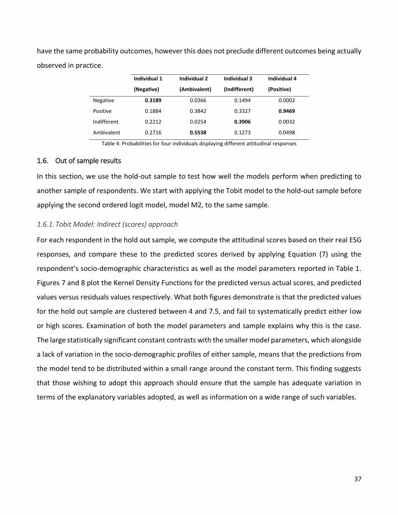
37

have the same probability outcomes, however this does not preclude different outcomes being actually

observed in practice.

Individual 1

(Negative)

Individual 2

(Ambivalent)

Individual 3

(Indifferent)

Individual 4

(Positive)

Negative 0.3189 0.0366 0.1494 0.0002

Positive 0.1884 0.3842 0.3327 0.9469

Indifferent 0.2212 0.0254 0.3906 0.0032

Ambivalent 0.2716 0.5538 0.1273 0.0498

Table 4: Probabilities for four individuals displaying different attitudinal responses

1.6. Out of sample results

In this section, we use the hold-out sample to test how well the models perform when predicting to

another sample of respondents. We start with applying the Tobit model to the hold-out sample before

applying the second ordered logit model, model M2, to the same sample.


For each respondent in the hold out sample, we compute the attitudinal scores based on their real ESG

responses, and compare these to the predicted scores derived by applying Equation (7) using the

respondent’s socio-demographic characteristics as well as the model parameters reported in Table 1.

Figures 7 and 8 plot the Kernel Density Functions for the predicted versus actual scores, and predicted

values versus residuals values respectively. What both figures demonstrate is that the predicted values

for the hold out sample are clustered between 4 and 7.5, and fail to systematically predict either low

or high scores. Examination of both the model parameters and sample explains why this is the case.

The large statistically significant constant contrasts with the smaller model parameters, which alongside

a lack of variation in the socio-demographic profiles of either sample, means that the predictions from

the model tend to be distributed within a small range around the constant term. This finding suggests

that those wishing to adopt this approach should ensure that the sample has adequate variation in

terms of the explanatory variables adopted, as well as information on a wide range of such variables.

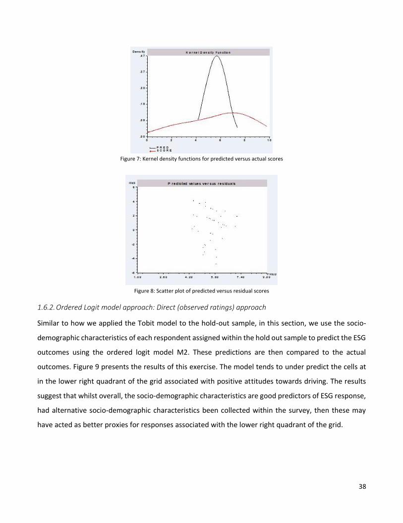
38

Figure 7: Kernel density functions for predicted versus actual scores

Figure 8: Scatter plot of predicted versus residual scores


Similar to how we applied the Tobit model to the hold-out sample, in this section, we use the socio-

demographic characteristics of each respondent assigned within the hold out sample to predict the ESG

outcomes using the ordered logit model M2. These predictions are then compared to the actual

outcomes. Figure 9 presents the results of this exercise. The model tends to under predict the cells at

in the lower right quadrant of the grid associated with positive attitudes towards driving. The results

suggest that whilst overall, the socio-demographic characteristics are good predictors of ESG response,

had alternative socio-demographic characteristics been collected within the survey, then these may

have acted as better proxies for responses associated with the lower right quadrant of the grid.

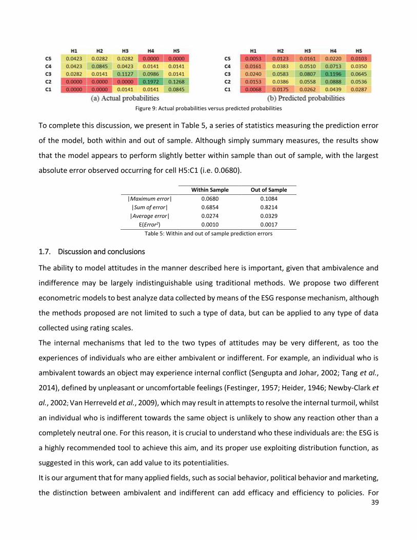
39

Figure 9: Actual probabilities versus predicted probabilities

To complete this discussion, we present in Table 5, a series of statistics measuring the prediction error

of the model, both within and out of sample. Although simply summary measures, the results show

that the model appears to perform slightly better within sample than out of sample, with the largest

absolute error observed occurring for cell H5:C1 (i.e. 0.0680).

Within Sample Out of Sample

|Maximum error| 0.0680 0.1084

|Sum of error| 0.6854 0.8214

|Average error| 0.0274 0.0329

E(Error2) 0.0010 0.0017

Table 5: Within and out of sample prediction errors

1.7. Discussion and conclusions

The ability to model attitudes in the manner described here is important, given that ambivalence and

indifference may be largely indistinguishable using traditional methods. We propose two different

econometric models to best analyze data collected by means of the ESG response mechanism, although

the methods proposed are not limited to such a type of data, but can be applied to any type of data

collected using rating scales.

The internal mechanisms that led to the two types of attitudes may be very different, as too the

experiences of individuals who are either ambivalent or indifferent. For example, an individual who is

ambivalent towards an object may experience internal conflict (Sengupta and Johar, 2002; Tang et al.,

2014), defined by unpleasant or uncomfortable feelings (Festinger, 1957; Heider, 1946; Newby-Clark et

al., 2002; Van Herreveld et al., 2009), which may result in attempts to resolve the internal turmoil, whilst

an individual who is indifferent towards the same object is unlikely to show any reaction other than a

completely neutral one. For this reason, it is crucial to understand who these individuals are: the ESG is

a highly recommended tool to achieve this aim, and its proper use exploiting distribution function, as

suggested in this work, can add value to its potentialities.

It is our argument that for many applied fields, such as social behavior, political behavior and marketing,

the distinction between ambivalent and indifferent can add efficacy and efficiency to policies. For

40

instance, in marketing identifying common individual characteristics which lead more likely to assess a

product or service both satisfying and unsatisfying, can suggest the producer on which cluster to focus

the efforts in order to increase the probability of satisfaction.

Thompson et al. (1995) modified the ambivalence index by Griffin in order to take into account two

different domains of ambivalence, cognitive and affective. A continuum of our research is to link two

(or more) ESGs, in order to relate different domains of ambivalence. Moreover, our additional interest

is to test whether and to what extent ambivalent and indifferent individual’s act differently (Costarelli

and Colloca, 2004; Yoo, 2010; Thornton, 2011) in a transport context, connecting attitudes towards

driving collected by means of ESGs and mode choices.

Two alternative approaches presented in this work are applied to ESG response type questions. Such

an instrument, different from traditional Likert and semantic differential type scales, allows the

researcher to detect various attitudinal outcomes towards an object, including ambivalence and

indifference, alongside the more commonly measured positive and negative attitudinal outcomes. To

date, whilst there exist several tools to measure ambivalence, including the use of subjective measures

(Priester and Petty, 1996; Clark et al., 2008), response time (Bargh et al., 1992; Fazio et al., 1986),

indices based on the scores of two separate semantic differential scales (Kaplan, 1972; Katz and Hass,

1988; Thompson et al., 1995), mouse tracking (Schneider et al., 2015), and scores captured in 2D space

using a bilinear model exploiting an ESG response mechanism (Audrezet et al., 2016), each of these

approaches have been criticized due to a number of potentially severe limitations. Subjective measures

may led to biased conclusions given respondents are able to easily provide socially desirable or

acceptable responses, whilst use of response times remains largely a black box, with little to no way

available to infer the true mental process resulting in attitudes. Mouse tracking studies remain hard to

replicate when many respondents are involved, and indices and scores whilst easy to implement,

assume that the response mechanism from which they are derived is a perfect measure of attitudes.

Assuming attitudes are latent constructs, and hence not directly measurable, the use of scores seems

anachronistic. For this reason, the models we suggest treat attitudes based on psychometric survey

questions as indicators of underlying latent psychological factors rather than as directly observed

measurements of said factors. An additional advantage of the proposed models, is their ability to

forecast future responses (i.e. predict out of sample). In many applied fields, such as environmental or

transport economics in which such psychological methods are commonly used, being able to predict

41

how attitudes may develop or change over time, or even what attitudes may exist in other non-sampled

populations, can support policy makers in their decisions.

Based on the Audrezet et al. (2016) scoring scheme, we use a Tobit model to demonstrate how such

scores can be appropriately modeled in practice. The Tobit model assumes an underlying latent

structure to predict the observed outcome, in this case the attitudinal score. The latent variable within

the model is predicted via socio-demographic variables. In the current chapter, whilst the model is

theoretically consistent with the view that attitudes are latent constructs, we find the model

performance to be somewhat lacking, providing poor predictive power. We argue however that this

finding is not the result of model misspecification but rather due to having a small number of socio-

demographic variables available for use, as well as a lack of variation in terms of the socio-demographic

variables we do have available.

We offer a second model, the ordered logit model, as an alternative means to model ESG response

data. By estimating two simultaneous ordered logit models, we demonstrate that it is possible to model

the observed outcomes of the grid, rather than a transformation of the observed outcomes. By

modelling the observed outcomes as opposed to an intermediary transformation, we show how it is

possible to model up to a probability, various attitudinal outcomes, something the Tobit model

struggles with. Within the chapter, we are able to demonstrate how alternative specifications of the

model can be used to test different theoretical frameworks associated with attitudes. In this vain, we

use the system of models to model (1) positive and negative items being driven by the same factors

exploiting a unique distribution function for both axes (e.g., if gender is positively significant, males

have a higher probability of scoring high positive and negative values than females), and (2) different

factors affect the positive and the negative items assuming total independence between them (e.g.,

being a male could lead more likely to higher values for positive item but could not have a significant

effect for the negative one), whilst in both cases allowing the unobserved factors to be related by means

of a correlation term. As with the Tobit model, we find selection of socio-demographic characteristics

is crucial to the predictive ability of the model.

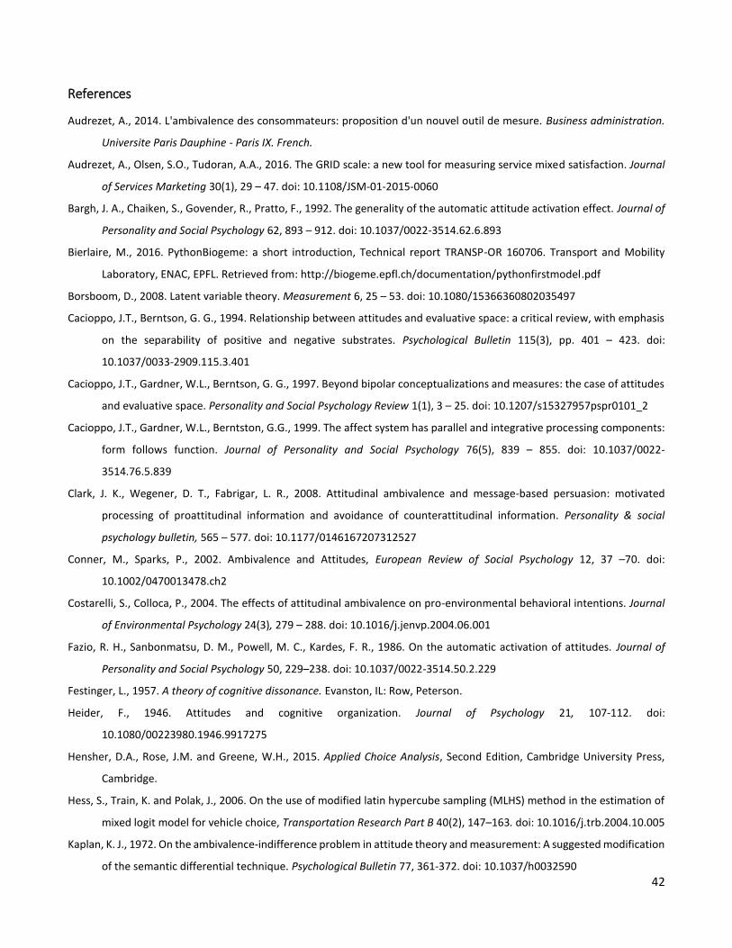
42

References

Audrezet, A., 2014. L'ambivalence des consommateurs: proposition d'un nouvel outil de mesure. Business administration.

Universite Paris Dauphine - Paris IX. French.



Bargh, J. A., Chaiken, S., Govender, R., Pratto, F., 1992. The generality of the automatic attitude activation effect. Journal of

Personality and Social Psychology 62, 893 – 912. doi: 10.1037/0022-3514.62.6.893

Bierlaire, M., 2016. PythonBiogeme: a short introduction, Technical report TRANSP-OR 160706. Transport and Mobility

Laboratory, ENAC, EPFL. Retrieved from: http://biogeme.epfl.ch/documentation/pythonfirstmodel.pdf

Borsboom, D., 2008. Latent variable theory. Measurement 6, 25 – 53. doi: 10.1080/15366360802035497


on the separability of positive and negative substrates. Psychological Bulletin 115(3), pp. 401 – 423. doi:

10.1037/0033-2909.115.3.401

Cacioppo, J.T., Gardner, W.L., Berntson, G. G., 1997. Beyond bipolar conceptualizations and measures: the case of attitudes

and evaluative space. Personality and Social Psychology Review 1(1), 3 – 25. doi: 10.1207/s15327957pspr0101_2

Cacioppo, J.T., Gardner, W.L., Berntston, G.G., 1999. The affect system has parallel and integrative processing components:

form follows function. Journal of Personality and Social Psychology 76(5), 839 – 855. doi: 10.1037/0022-

3514.76.5.839

Clark, J. K., Wegener, D. T., Fabrigar, L. R., 2008. Attitudinal ambivalence and message-based persuasion: motivated

processing of proattitudinal information and avoidance of counterattitudinal information. Personality & social

psychology bulletin, 565 – 577. doi: 10.1177/0146167207312527

Conner, M., Sparks, P., 2002. Ambivalence and Attitudes, European Review of Social Psychology 12, 37 –70. doi:

10.1002/0470013478.ch2



Fazio, R. H., Sanbonmatsu, D. M., Powell, M. C., Kardes, F. R., 1986. On the automatic activation of attitudes. Journal of

Personality and Social Psychology 50, 229–238. doi: 10.1037/0022-3514.50.2.229

Festinger, L., 1957. A theory of cognitive dissonance. Evanston, IL: Row, Peterson.

Heider, F., 1946. Attitudes and cognitive organization. Journal of Psychology 21, 107-112. doi:

10.1080/00223980.1946.9917275

Hensher, D.A., Rose, J.M. and Greene, W.H., 2015. Applied Choice Analysis, Second Edition, Cambridge University Press,

Cambridge.

Hess, S., Train, K. and Polak, J., 2006. On the use of modified latin hypercube sampling (MLHS) method in the estimation of

mixed logit model for vehicle choice, Transportation Research Part B 40(2), 147–163. doi: 10.1016/j.trb.2004.10.005



https://dx.doi.org/10.1207/s15327957pspr0101_2

https://dx.doi.org/10.1080/00223980.1946.9917275

http://dx.doi.org/10.1037/h0032590

43

Katz, I., Hass, R. G., 1988. Racial ambivalence and American value conflict: Correlational and priming studies of dual cognitive

structures. Journal of Personality and Social Psychology 55, 893–905. doi: 10.1037/0022-3514.55.6.893



Likert, R., 1932. A technique for the measurement of attitudes. Archives of Psychology, R. S. Woodworth Editor, 140, New

York.

Newby-Clark, I.R., McGregor, I., Zanna, M.P., 2002. Thinking and caring about cognitive inconsistency: When and for whom

does attitudinal ambivalence feel uncomfortable? Journal of Personality and Social Psychology 82, 157-166. doi:

10.1037/0022-3514.82.2.157

Osgood, C. E., 1964. Semantic differential technique in the comparative study of cultures. American Anthropologist 66(3),

171 – 200. doi: 10.1525/aa.1964.66.3.02a00880

Priester, J.R., Petty, R.E., 1996. The gradual threshold model of ambivalence: relating the positive and negative bases of

attitudes to subjective ambivalence. Journal of Personality and Social Psychology 71, 431–449. doi:10.1037/0022-

3514.71. 3.431

Russell, J. A., Carroll, J. M., 1999. On the bipolarity of positive and negative affect. Psychological Bulletin 125, 3–30.

Schneider, I.K., van Harreveld, F., Rotteveel, M., Topolinski, S., van der Pligt, J., Schwarz, N., Koole, S.L., 2015. The path of

ambivalence: tracing the pull of opposing evaluations using mouse trajectories. Front. Psychol. 6(996). doi:

10.3389/fpsyg.2015.00996

Schwarz, N., Bohner G., 2001. The construction of attitudes. Manuscript of a chapter in A. Tesser and N. Schwarz.

Intrapersonal processes, Blackwell Handbook of Social Psychology, 436 – 457. Oxford, UK. Blackwell.

Sengupta, J. Johar, G.V., 2002. The effects of inconsistent attribute information on the predictive value of product attitudes:

toward a resolution of opposing perspectives. Journal of Consumer Research 29(1), 39-56. doi: 0093-

5301/2003/2901-0003

Tang, T., Fang, E. Wang, F., 2014. Is neutral really neutral? The effects of neutral user-generated content on product sales.

Journal of Marketing 78(4), 41-58.

Tay, L., Kuykendall L., 2017. Why self-reports of happiness and sadness may not necessarily contradict bipolarity: a

psychometric review and proposal. Emotion Review 9(2), 146-154. doi: 10.1177/1754073916637656.

Thompson, M.M., Zanna, M.P. and Griffin, D.W., 1995. Let’s not be indifferent about (Attitudinal) ambivalence. In Petty, R.E.

and Krosnick, J.A. (Eds), Attitude Strength: Antecedents and Consequences, (pp. 361-386) Lawrence Erlbaum,

Mahwah, NJ.



Thurstone, L.L., 1928. Attitudes can be measured. American Journal of Sociology 33, 529 – 554.

Van Herreveld, F., Van der Pligt, J., De Liver, Y., 2009. The Agony of Ambivalence and Ways to Resolve It: Introducing the

MAID Model. Personality and Social Psychology 13(45). DOI: 10.1177/1088868308324518.

44


72(1), 163-177. doi: 10.1017/S0022381609990545

45

Chapter 2. The implementation of the Evaluative Space Grid in a hybrid choice

model to overcome the disadvantages of measuring attitudes using common

scales.

Antonio Borriello1, Stefano Scagnolari1

1Università della Svizzera italiana

Abstract

The study of latent variables, and in particular of attitudes, contributes to a better

understanding of individual preferences and behavior and it is now common practice

within transportation literature. However, the procedure of attitude measurement is

still not optimal. Two major issues are the misspecification of the attitude itself and

in the number of suitable items used for defining the psychological factor. The

incorrect measurement entails a poor representation of individuals on the latent

continuum and a less precise definition of the latent variable itself.

These issues become even more relevant when a Likert scale is used. Indeed, the

neutral point of this scale is selected by both individuals having an ambivalent and an

indifferent attitude, and the poor representation makes impossible to distinguish

these categories. Nevertheless, such a distinction can be very profitable for policy

reasons. To overcome this issue and to suggest more effective policies, we propose

using the Evaluative Space Grid (ESG), which is a single-item measure of positivity and

negativity, to collect attitudinal variables. This tool can distinguish between

individuals with indifferent and ambivalent attitudes, as well as those with positive

and negative inclinations.

This work models the ESG using a pair of ordered logit regressions and suggests a

procedure to include this approach in the framework of hybrid choice models.

Furthermore, it endeavors to shed light on the preferences of individuals having

indifferent and ambivalent inclinations in a transportation context, showing the

hypothesis that their preferences are different for commuting trips.

Keywords: Attitude measurement, hybrid choice model, Evaluative Space Grid, Ambivalence, Indifference.

46

2.1. Introduction

The integration of psychological factors in transportation literature is a fundamental key for

understanding individual behavior. In the last two decades, hybrid choice models, which explore the

influence of attitudes on individuals’ choices as well as their composition, became quite popular and

widespread. In this work we focus on a new way of measuring an attitude with the scope of exploring

individuals’ behavior and the choices they make in a transportation context.

Psychologists define an attitude as "the sum-total of a man's inclinations and feelings, prejudice or bias,

preconceived notions, ideas, fears, threats and convictions about any specific topic” (Thurstone and

Chave, 1929). From an econometric point of view, an attitude is a variable that cannot be directly

measured (latent) but that can be defined through some indicators (or observable variables) net of an

error. The first attempt to measure an attitude was made by Thurstone (1928), who measured the

inclination towards prohibition, pacifism/militarism, and religion. Thurstone developed between eighty

and one-hundred statements and asked subjects to place each statement on an 11-point scale defined

by a central neutral point, with five points located to either side. Likert (1932) refined Thurstone’s work

and proposed a scale based on the measurement of different statements (items) of which subjects were

asked to express their level of agreement/disagreement. At the present time, this instrument is

considered being the gold standard for measuring attitudes and it is the most common tool in

psychology or in applied fields like transportation.

Because of their latent nature, the higher the number of observable variables suitable to measure the

attitude, the lower the error computed in the measuring process. Consider as an example the

measurement of passengers’ loyalty to public transport modes. Shiftan et al. (2015) measure this

attitude using twenty-six items representing affective, conative, action and cognitive facets of loyalty,

as well as hedonic value, comfort, convenience and reliability. The assessment of the latent variable

“loyalty to public transport modes” depends on how much variance of that attitude the items are able

to explain. Omitting constructs such as e.g. comfort or reliability would increase the randomness of the

latent variable and, as a consequence, reduce its efficacy.

The use of a limited number of measurable items for defining an attitude and the misspecification of

the attitude itself are the main problems emerging in several papers in transportation mode choice.

Indeed, researchers who focus on the study of attitudes from a psychological perspective generally

exploit a larger set of suitable items for defining a latent construct than researchers who model the

47

behavioral consequences of the attitudes. In a study aimed at segmenting “the population of day trip

travelers into potential ‘mode switchers’ using cluster analysis”, Anable (2005) employs respectively

twenty-four and twenty-seven items to represent the general attitude towards the car and its

alternatives. In an application of the Theory of Planned Behavior designed to understand the factors

influencing the car use for commuting, Abrahamse et al. (2009) assess the general attitude towards the

car using a set of seven items. The attitude pro-car is instead defined by Atasoy et al. (2012) by using

three items in a hybrid choice model with latent classes for a sample of Swiss respondents. The

observable variables adopted to proxy the latent construct, measure two specific aspects of the attitude

(convenience and flexibility of the car) and therefore, several important aspects were not included in

the construction of the attitude, decreasing its explained variance. Analogous differences on the

number of items used, can be found for the definition of the attitude “environmental concerns”, which,

referring to the papers by Mokhtarian et al. (2001), Ory, Mokhtarian (2005), Anable (2005), Prillwitz

and Barr (2011), has been defined using on average 8 items, whilst Johansson et al. (2006), Atasoy et

al. (2012), Hess et al. (2013) and Bahamonde-Birke, Hanappi (2016), employ on average 4.5 items to

outline the same attitude. Rundmo et al. (2011) define the safety perceived for public and private

means using five and seven items respectively, whereas Daziano and Bolduc (2013), and Raveau et al.

(2010) use only two items to explore the same latent constructs. The general satisfaction with public

transport and soft modes has been explored by Prillwitz and Barr (2011), who use ten and nine items

respectively, whereas a general satisfaction for commuting has been measured using one item by Abou-

Zeid and Ben-Akiva (2011).

An inappropriate specification of the attitude can be observed in the study by Domarchi et al. (2008),

who investigate the effect of the attitudes towards car and public transport on mode choice by means

of two items. Using “direct measure” of what actually is a latent construct, they generate high

aggregation of contents. Indeed, respondents can associate the question “For me, using car / public

transport to arrive to work is good’’ with several aspects, like its convenience, its flexibility and its cost

inter alia. A similar misspecification of the latent variable can be also found in Bolduc et al. (2008) and

Bolduc and Daziano (2010), who use a considerable number of items (eight) to define the “appreciation

of new car features”, but who measure directly “safety” and “reliability”, which clearly are latent

variables. It is also a common practice to treat a latent construct as an attribute of the choice

48

experiment: for instance, Espino et al. (2003) and Espino et al. (2006) define “comfort” as an attribute

with generic categories “low – standard or medium – high”.

In order to validate a new scale for measuring an attitude, psychologists consider numerous items

related to it and then, using techniques of variable reduction, cut out the less informative indicators.

The main reason why choice modelers employ a limited number of items concerns the way the survey

is designed in a choice experiment setting: the questionnaire usually contains a section with six/ten

choice tasks as well as sociodemographic questions. The addition of a long list of attitudinal indicators

would make the filling of the survey time consuming and quite demanding, affecting the quality of the

responses, as well as (and maybe mainly) the cost for distributing the survey (using an internet panel,

respondents are paid according to the time spent completing the questionnaire). Furthermore, many

researchers are not aware of the existing literature in transportation psychology and the list of items

useful for identifying the attitude is usually discussed within a focus group with experts in the field, who

are choice modelers themselves and rarely psychologists. A further difference between the definition

of a scale in psychology and choice modeling consists in the positioning of the items along the latent

continuum. Psychologists include items with a positive, neutral and negative valence covering the entire

latent continuum domain (i.e. they use appropriate wording aimed at capturing a possible positive,

neutral and negative outcome of the attitude), whilst choice modelers usually use items with an

extreme positive or a negative valence.

The lower discrimination and information lead to an aggregation of individuals with an indifferent or

ambivalent attitude in choice modeling applications. Indeed, the central value on a Likert scale can

express indifference as well as ambivalence. Indifference implies that an individual has no interest in

the stimuli being studied, revealing a low positive and negative reaction; ambivalence, on the other

hand, suggests that the subject experiences both a moderate or high positive and negative valence

towards the stimuli. A correct distinction between these two categories of respondents is fundamental

for understanding behavior and suggesting more effective policies. As a matter of fact, it has been

shown that indifferent and ambivalent individuals act differently in contexts such as political elections

and environmental behavior (Costarelli and Colloca, 2004; Yoo, 2010; Thornton, 2011).

In this chapter, we propose to measure attitudes using a different tool, namely Evaluative Space Grid

(ESG, Larsen et al., 2009), rather than the Likert scale, to allow the differentiation between ambivalence

and indifference, as well as positive and negative attitudes. This work has a twofold ambition: from a

49

theoretical perspective, it endeavors to integrate the ESG in the framework of discrete choice modelling

in order to avoid the aggregation of individuals positioned on the neutral part of a latent continuum;

the empirical contribution concerns testing the hypothesis that individuals with indifferent and

ambivalent attitudes towards the private car use for commuting behave differently in the context of

transport mode choice.

The remainder of the chapter is organized as follows. In the next sections, we first introduce the ESG

tool, proposed by Larsen et al., and the methodology, which elucidates the econometric steps to define

a hybrid choice model including the evaluative space grid, and we then present the sample, the survey

as well as the model we use to analyze it. The following section shows the results obtained through the

hybrid choice model and in particular the differences amongst different categories of respondents,

namely those including individuals with a positive, negative, indifferent and ambivalent attitude

towards the private car use for commuting trips. We conclude the chapter summarizing the major

evidence and discussing the benefits of using the evaluative space grids in a hybrid choice model in the

context of transport.

2.2. Evaluative Space Grid (ESG)

The studies on the neutral part of the latent continuum started decades ago and the first attempt to

measure ambivalence was made by Kaplan (1972) who derived a simple formula using the respondents’

assessment of a Likert item. However, the common Likert scale is not suitable to measure ambivalence

and indifference, even if it contains items with both a positive and a negative valence. Indeed, the use

of sequentially structured conversely framed questions has been criticized within the literature given

that such an approach has the potential to induce subjects to reveal distorted preferences, particularly

if for the second set of questions they attempt to display consistent answers with the preferences given

to the first set of questions asked. For this reason, Larsen et al. proposed using a “single-item measure

of positivity and negativity” which they termed the evaluative space grid. The ESG is designed to recover

the independent and simultaneous assessment of positive/negative attitudes towards an object, and

has since been validated in different fields such as psychology and social behavior (e.g., Audrezet, 2014;

Audrezet, Olsen and Tudoran, 2016). This tool follows the theoretical framework of Evaluative Space

Model (ESM) proposed by Cacioppo and Bernston (1994), who suggested that positive and negative

feelings can be experienced at the same time, also with strong intensities.

50

The ESG contrasts positive and negative stimuli towards an attitude, posing two 5 points scales on x

and y axes. Subjects are asked to select one of over 25 cells that best reflects their simultaneous

negative and positive feelings towards the stimulus under study, as shown in Figure 1. The grid is

designed to differentiate between four different attitudes: (1) positive (high positive and low negative),

(2) negative (low positive and high negative), (3) indifference (low positive and negative), and (4)

ambivalence (moderate to high positive and negative).

Figure 1: Evaluative space grid. Audrezet (2014) suggests the following division of the grid: bottom left cells identify an indifferent

individual (yellow); bottom right cells classify a subject with a positive attitude (green); the top left cells (red) categorize an individual with a negative attitude; top right cells identify a subject with an ambivalent attitude.

2.3. Methodology

In this section, we discuss the methodology applied to incorporate the Evaluative Space Grid in a choice

model framework. To model the ESG, we use two ordered logit regressions which take into account the

ordinal nature of the tool. Three types of relationships are defined in the hybrid discrete choice model

as follows.

Let consider n respondents who face a choice set composed by J alternatives. The chosen alternatives

is 1argmax(( ( , , , ; , , , ) | 1,..., ; 1,..., )n nj j n j n njk U f X W Y G a d c n N j J , where jX is a vector of attributes for

alternative J, nW represents a vector of socio-economic variables describing individual n, nG indicates

the vector of l latent variables, whilst the matrix jY defines which latent variables are inserted in the

utility function of alternative J. The impacts of these latent variables are measured by the vector c,

whilst vectors a and d represent the impact that attributes and socioeconomic variables have on the

51

utility of the alternative respectively. The error term nj is i.i.d. extreme value type 1. The analyst can

define the function 1( )f g according to the data.

Latent variables are determined by a series of structural relationships. We assume that they may be

explained, or proxied, by observable data, such as gender, income, etc.. However, given that such data

are not fully capable of explaining an individual’s attitudes towards an object, we decompose nlG in two

parts, an observed component and a stochastic component, such that nl nl nlG O . For simplicity, we

assume a linear additive specification for the observed component of the latent variable, such that

nl nlO bW where nlW represents the vector of socio-demographic characteristic of subject n associated to

the latent variable l , and b is the vector containing the marginal contribution to the latent variable

associated with the socio-demographic characteristics. The remaining term nl is a stochastic term

representing the idiosyncratic impact on nlG , not directly modelled in nlO , following a Normal

distribution with zero mean and variance 2

l .

Attitudinal response niy for the ith indicator variable (or item) is a categorical variable modelled by a

measurement equation, whose general formulation is ni i i n niy d G , where i is a constant, nG is

the vector of the latent variables whose effect on the response is measured by the vector id (note that

this vector may contains zero values if the latent variables do not have an impact on a given item). The

specification of ni determines the type of measurement model: through this work we assume that i

is distributed as extreme value type 1 over the population for any item and, therefore, we use an

ordered logit to model the attitudinal responses. Hence, the level of nlG determines the observed

responses such that if nlG exceeds some psychological threshold, ,irl category r will be selected, else

one of the preceding categories will be chosen.

Assuming a five category scale, the probability that respondent n will choose category r for item i is

1

1

1

1

4

4

exp( ), 1

1 exp( )

exp( ) exp( ), 1 5,

1 exp( ) 1 exp( )

exp( )1 , 5.

1 exp( )

i l ni

i l ni

irl ni irl ninir

irl ni irl ni

i l ni

i l ni

Or

O

O OP r

O O

Or

O

(1)

52

Equation (1) suggests that each response can be chosen up to a modelled probability for any given

respondent. That is, for each response category associated with response item i, we estimate the

probability distribution for all possible outcomes for each respondent n. We define an indicator variable

nir , such that 1nir if category r is chosen by individual n for item i and 0 otherwise.

Up to this point, we followed the methodology described in Daly et al. (2012). However, in this work

we collect the attitudes using the Evaluative Space Grid response mechanism, rather than a common

Likert scale, to allow simultaneous assessment of positive and negative attitudes towards the object

under study. Therefore, we capture two discrete outcomes per any grid, niy and

niy , representing the

concurrent positive and negative dimensions of the attitude for item i respectively. Both the positive or

negative dimensions are assumed to provide a discrete representation of two separate, yet potentially

correlated, continuous latent variables, nl nl nlG b W and nl nl nlG b W . The modelling approach we

propose follows the assumption of the ESM, which allows for the possibility that positive and negative

attitudes arise from different psychological processes. In order to explain the observed positive and

negative responses for the same stimuli, we use different subsets of socio-demographic characteristics

(nlW and

nlW ). We further extend the modelling framework to allow a pattern of possible correlation of

the stochastic components of nlG and nlG . We do this by constructing the random terms of the positive

and negative components of the latent variables as

nl nlt (2a)

2* ( 1 )nl nl nlt t (2b)

where nlt and nlt are random draws following a Normal distribution with zero mean and unit variance

(note that nl still follows the same distribution). Given that neither nl and nl are associated with an

observable variable, both terms represent additional sources of error associated with nlG and

nlG

respectively, with correlation equal to . To estimate the additional error structure, we rely on a

Cholesky decomposition.

Two discrete outcomes are modelled in the measurement equations, such that

ni i i n niy d G (3a)

ni i i n niy d G (3b)

53

Positive (negative) outcome, ( )ni niy y , depends on the positive (negative) domain of the latent variable,

( )n nG G and its effect on the attitudinal response is measured through the vector ( )i id d . Under this

scenario, it is possible to treat irl irl or

irl irl , the outcome of which should be determined empirically.

The objective of the analyst is to estimate the parameters included in the three types of relationships.

However, for identification issues, it is necessary to impose some constraints. First, the normalization

of the scale for the measurement equation should be considered. Ben-Akiva et al. (1999) suggested to

normalize to 1 the impact of one the attitudinal indicators id (

id ) of each of the latent variables and

estimate the variances of the errors in the structural equation ( 2

); Bolduc et al. (2005) instead,

proposed to normalize the variances to 1 and to estimate id (id ) for the whole set of indicators.

Second, the simultaneous estimation of the constants i ( i

) in the measurement equations and the

first threshold 1i l (1i l ) used in the ordered logit is unfeasible and therefore only one of the two

parameters should be included into the model.

With the above background, we define the probability of observing subject n selecting the ( )th thr s

response category for item ( )i i conditional on latent variables and hence on (variance-covariance

matrix of ,nl nl ) as

5

1

( | ) nir

ni nir

r

P y G P

(4a)

5

1

( | ) nis

ni nis

s

P y G P

(4b)

The conditional and unconditional probabilities of observing individual n selecting the vector of

responses ( )n ny y are defined as

1

( | )I

n ni

i

P y G y

(5a)

1

( | )I

n ni

i

P y G y

(5b)

( ) ( | )n nP y P y G dF

(6a)

.( ) ( | )n nP y P y G dF

(6b)

where ( )F F

is the distributions of ( ) .

54

The unconditional probability of observing subject n choosing the jth alternative is:

( ) ( | , )n nP j P j G G dF dF

(7)

where ( | , )nP j G G is the individual probability conditioned on the latent variables G and G

. It follows

that the unconditional joint probability of observing subject n choosing the jth alternative and selecting

the vector of responses ( )n ny y is

( ) ( ) ( )n n n nP P j P y P y (8)

or, if the researcher assumes independency among any ESG and the choice model, it is possible to

integrate after the product,

( | , ) ( | ) ( | )n n n nP P j G G P y G P y G dF dF

(8b)

The final log-likelihood function is therefore

1

log( )N

n

n

LL P

(9)

Given that the integrals in equation 7 do not have a closed form, simulated maximum likelihood

estimation has to be used to locate the parameters of interest.

2.4. Empirical data

In this section we present the sample and the types of data we used for the analysis. The survey contains

a stated preference experiment on transportation mode choice consisting in six choice tasks and three

evaluative space grids employed to collect attitudes towards commuting to work or university by a

private car.

2.4.1. Sample composition

Data was collected from September 2014 to September 2016 in Lugano, Lausanne and Zurich, three

different cities in Switzerland representing three different linguistic parts of the country, Italian, French

and German respectively. Using a paper and pencil questionnaire, a sample of 595 respondents were

interviewed about their attitudes towards car use and their preferences for commuting trips. The

sample is mainly composed by university students (87%), with the remainder being either workers or

apprentices. In the present work, the focus on younger respondents (the mean age of the sample is

55

21.9) occurred for two reasons. First, experience suggests that it is easier to collect data from students;

second, younger respondents display a higher degree of heterogeneity in terms of travel behavior, and

use alternative commuting modes more frequently than older respondents, generating more valuable

information (see e.g., Whalen et al., 2013; Khattak et al., 2011). Fifty-five percent of respondents are

male and large part of the sample lives either in the Italian or French speaking areas (39 and 37 percent

respectively), with the remainder living in the German speaking area (13 percent) and abroad (11

percent). The majority of the respondents reports not having any earnings (49 percent) or earning less

than 30,000 CHF/year (40 percent). Eighty-three percent of the sample reports having access to a car

in their household, with the average number of days in which the car was in use (with the respondent

acting as either the driver or as a passenger) being equal to 2.81 days per week. The average number

of days per week in which respondents do sports (any activity, individual or collective, that lasts for at

least 30 minutes) is 2.44.

2.4.2. Structure of the questionnaire: SP experiment

The questionnaire includes a specific section with a stated preference experiment, consisting of the

mode choices for a commuting trip: respondents are asked to imagine a near future (five years) in which

they live in the city where they have been interviewed, have a position consistent with their education

and have to work in the city center. Every morning they are assumed to commute for a distance equal

to the average commuting distance (Mikrozensus Mobilität und Verkehr, 2010) which is respectively

2.6, 4.3 and 4.45 km (one way) in Lugano, Lausanne and Zurich. Travel time, monthly cost and the

transport system densities, as well as a hypothetical wage that respondents would earn, vary across

choice tasks. We collect individual preferences looking at a near future for two main reasons: first, we

tried to make the framework more realistic given that the set of alternatives includes an innovative but

inexistent transportation system, namely moving walkways; second, given that the sample is mainly

composed of students who do not earn any (or do earn low) wages, we can have insights on the impact

of expected wages on transportation mode choice.

Eight transportation modes compose the set of alternatives, however respondents can only choose

among a subset of them. The group of private alternatives comprises private car (PC), motorbike (MO),

electric bike (EB) and conventional bike (BI) and it varies among respondents. The set of public modes

includes bus, train and metro (aggregated as a unique alternative and labelled PT), car-sharing (CS),

56

carpooling (CP), moving walkways (MW) and is the same for any respondent. The moving walkways

system is an innovative transportation mode which is described to be installed on the main sidewalks

of the city, totally free and uncovered. Its width allows two passenger lanes and the length is 200 m on

average (in order to allow to get off and on), with a speed varying between 12 and 15 km/h. We consider

carpooling as public mode in a sense that it is not a “purchasable-private” alternative. The set of

alternatives is kept constant among choice tasks for the same respondent. Table 2 contains different

combinations of private alternatives, which can be presented to the respondents. We do not include

the combinations “motorbike + e-bike/bike” and “e-bike + bike” because we expect one alternative to

be dominant. For example, in a situation in which an individual is asked to choose between e-bike and

bike for commuting, the latter alternative is dominated, generating no valuable information.

1 Private car + conventional bike

2 Motorbike

3 E-bike

4 Private car + motorbike

5 Private car + e-bike

6 Conventional bike

Table 2: Different set of alternatives.

Three attributes describe the alternatives: monthly cost (CST), one-way travel time (TT) and move or

being moved (DST) are defined by three levels, different for Lugano, Lausanne and Zurich. The monthly

cost comprises the purchase and maintenance costs for MO, BI and EB, whilst for PC and CP it includes

the parking cost in the city center, as well the purchase and maintenance costs. The DST is a proxy of

the system density indicating the walking km needed to cover the commuting distance. Furthermore,

any choice task presents a value representing the monthly wage defined accordingly to the median

wage (± 25%) for workers five years after obtaining a master degree (in any field).

The software Ngene 1.1.2 (Ngene, 2014) is used to compute an efficient design (Rose et al., 2008; Rose

and Bliemer, 2008) with two blocks. To avoid very unreal situations, we exclude from the design

combinations with the highest value for DST and the lowest for TT for public transport and moving

walkway. We design twelve choice tasks (six for each block) for any subset of alternatives. The same

procedure is used for the three different cities, generating 3 (cities) * 6 (combinations) different

designs. The resulting D-errors range from 0.002 (private car + conventional bike combination in

Lausanne) to 0.05 (private car + e-bike combination in Lausanne). Summarizing, any respondent faces

57

six choice tasks, according to the city, the combination of private means and the block to which he or

she is randomly assigned. Table 3 shows an example of a choice task for a respondent living in Lugano.

Monthly wage: 7500 CHF

Public Transport

Conventional bike

Moving Walkway

Private car Car-sharing Car-pooling

Travel time

14 min 10 min 23 min 14 min 20 min 21 min

Monthly Cost

45 CHF/ month

4 CHF/ month

free 260 CHF/

month 190 CHF/

month 80 CHF/ month

Move or being

moved

1.0 walking km

Whole route by bike

1.0 walking km

0.2 walking km

1.0 walking km

0.3 walking km

Choice □ □ □ □ □ □

Table 3: example of choice task for a respondent living in Lugano, whose set of private alternatives contains a private car and a

conventional bike

2.4.3. Structure of the questionnaire: attitudinal questions

The second section of the survey contains attitudinal questions measured using the evaluative space

grids. This tool is quite recent and it is not commonly employed in surveys aimed at measuring attitude.

To make sure that respondents could complete the questionnaire in a proper way, a trained interviewer

provided a verbal description of the task and demonstrated the process via an example that was not

related to the topic of interest. Overall, respondents completed six ESGs, three of which are used here

and are framed with the statement “Depending on your experience, you think that driving is…”. In

completing the six ESGs, respondents were asked to consider only commuting trips (to university or

workplace). The full list of the three pairs of adjectives includes flexible vs binding, comfortable vs

uncomfortable, and handy vs challenging.

A pre-pilot and pilot of the instrument (involving 80 students from Univeristà della Svizzera italiana)

found that respondents were hardly able to understand two of the three adjective pairs in the context

of a commuting trip. Indeed, flexible vs binding, and handy vs challenging, were found to be less obvious

to respondents. As such, the meaning of these two pairs was emphasized during the survey, with

respondents informed that flexible vs binding referred to whether it was possible or not to change a

selected route mid trip as a result of changing circumstances such as in the case of an accident, whilst

handy vs challenging referred to more practical issues such as the timing for leaving home, ease of

locating parking, and whether it is necessary to transfer to a different transport mode during the trip.

An example grid is given in Figure 2.

58

Figure 2: Example of ESG in the survey

The distribution of the responses for the evaluative space grids used for the subsequent analysis is

displayed in Figure 3. In contrast to the Evaluative Space Model suggested by Cacioppo and Bernston

(1994), Tay and Kuykendall (2017) proposed an “updated bipolar model” according to which individuals

who experience moderate amounts of happiness can also experience moderate sadness, but mixed

feelings are less likely to co-occur with strong intensities. Indeed, authors reported that in their

experiment only 7 out of 166 respondents had an ambivalent emotion. The distribution of the

responses in this experiment shows a very distant pattern and confirms the Evaluative Space Model.

Specifically, 43 percent, 31 percent and 37 percent of respondents reported considering commuting by

car moderate-high flexible/binding, comfortable/uncomfortable and handy/challenging, respectively.

BIN

DIN

G

5 2.2% 2.0% 0.8% 0.2% 1.0%

UN

CO

MFO

RTA

BLE

5 4.2% 1.5% 0.7% 0.7% 1.2%

CH

ALL

ENG

ING

5 3.0% 1.8% 0.5% 0.7% 0.3%

4 1.0% 6.6% 4.2% 6.1% 1.8%

4 0.8% 7.2% 3.2% 2.2% 0.7%

4 1.2% 7.6% 4.5% 3.7% 0.5%

3 0.3% 1.3% 13.3% 9.2% 6.2%

3 0.2% 2.7% 12.3% 7.4% 2.9%

3 0.7% 4.0% 13.6% 11.9% 1.7%

2 0.2% 1.5% 2.7% 14.6% 10.6%

2 0.0% 1.8% 2.5% 18.2% 8.4%

2 0.0% 1.7% 2.4% 15.3% 8.4%

1 0.8% 0.2% 0.8% 2.2% 10.1%

1 0.2% 0.0% 0.8% 4.2% 16.1%

1 1.2% 0.0% 2.0% 3.7% 9.6%

1 2 3 4 5 1 2 3 4 5 1 2 3 4 5 FLEXIBLE COMFORTABLE HANDY

Figure 3: distribution of responses for the ESGs.

59

2.5. The model

Before running a hybrid choice model, we perform a factor analysis on the items collected using the

grids (flexible, binding, comfortable, uncomfortable, handy and challenging) in order to properly design

the latent construct. The analysis shows that flexible and binding do not belong to the same latent

construct as they show high values of uniqueness and therefore they are removed from the analysis.

The second column in Table 4 reports the coefficients of the four remaining items: comfortable and

handy have a positive impact on the latent variable practicality and convenience of using the private

car for commuting purposes, whilst uncomfortable and challenging have a negative effect. In other

words, an individual who assigns a higher value to the items comfortable and handy (uncomfortable

and challenging), is more likely to assess commuting by car practical and convenient (impractical and

inconvenient). The internal consistency of the construct is measured through Cronbach’s alpha which

is large enough, meaning that the items explain the same construct.

Variable Practicality Uniqueness

Comfortable 0.8061 0.3501

Uncomfortable -0.7862 0.3818

Handy 0.7087 0.4978

Challenging -0.6675 0.5545

Cronbach’s alpha 0.8317

Table 4: Exploratory factor analysis.

Items flexible and binding are removed as they present a high value of uniqueness.

Following the evidence of the exploratory factor analysis which suggests a unique factor, we create two

opposite domains of the same latent variable (nG and

nG ), as explained in the methodology section.

Specifically, two latent variables measure the positive and the negative realms of practicality and

convenience of using the private car for commuting purposes, respectively. A different set of socio-

economic variables explain the latency in the structural equations:

_ ___ * * _age c use Ita Pub Fusen n n n Fr Sp nG b Age b Car use b Ita b Fre Spo b Pub Fr use (10a)

_ __ _

pri c use car avn stud nG b Pri b Car use b Car av b Stud (10b)

The practicality and convenience of using the private car for commuting purposes is function of age,

number of days of car use per week, a dummy variable representing native Italian speakers, the

interaction between native French speakers and the number of days of sport as well as a further

60

interaction indicating respondents who commute with a public mean but who use the private car

frequently (more three or more days per week, both as a passenger or driver). The latent variable

measuring the impracticality and inconvenience of using the private car for commuting purposes,

instead, depends on a dummy variable equals to 1 if the respondent actually commutes by a private

mean, the number of days of car use per week (note that we specify two different parameters in

equations (10a) and (10b)), car availability and student status. We adopt the normalization suggested

by Bolduc et al. and, as a consequence, we only estimate the effects of the socio-economic variables

on the latent variables and we fix the standard deviation of the error terms to one. Nevertheless, the

parameter capturing the correlation between the positive and negative domains of the latent variable

is estimated.

The latent variable nG explains the observable items comfortable and handy, whilst uncomfortable and

challenging depend on nG . Different psychological thresholds are set for different latent variables.

Furthermore, to allow a more flexible and congruent specification of the link between the latent

variable and the related items, we set specific psychological thresholds in the measurement equations,

hypothesizing that the same value of the latent construct can correspond to different categories for

different related items. As a matter of example, Figure 4a shows the value that an individual has on the

positive domain of the latent variable practicality (3.56), which corresponds to category 5 on the

measurable variable comfortable and to category 4 on handy. The psychological thresholds for the

negative domain are also different from the ones used for the positive realm (Figure 4b). In total, the

number of thresholds to be estimated in the model is given by the number of items * the number of

categories per item – 1, that equals to 4 * (5 – 1) = 16 in our specification.

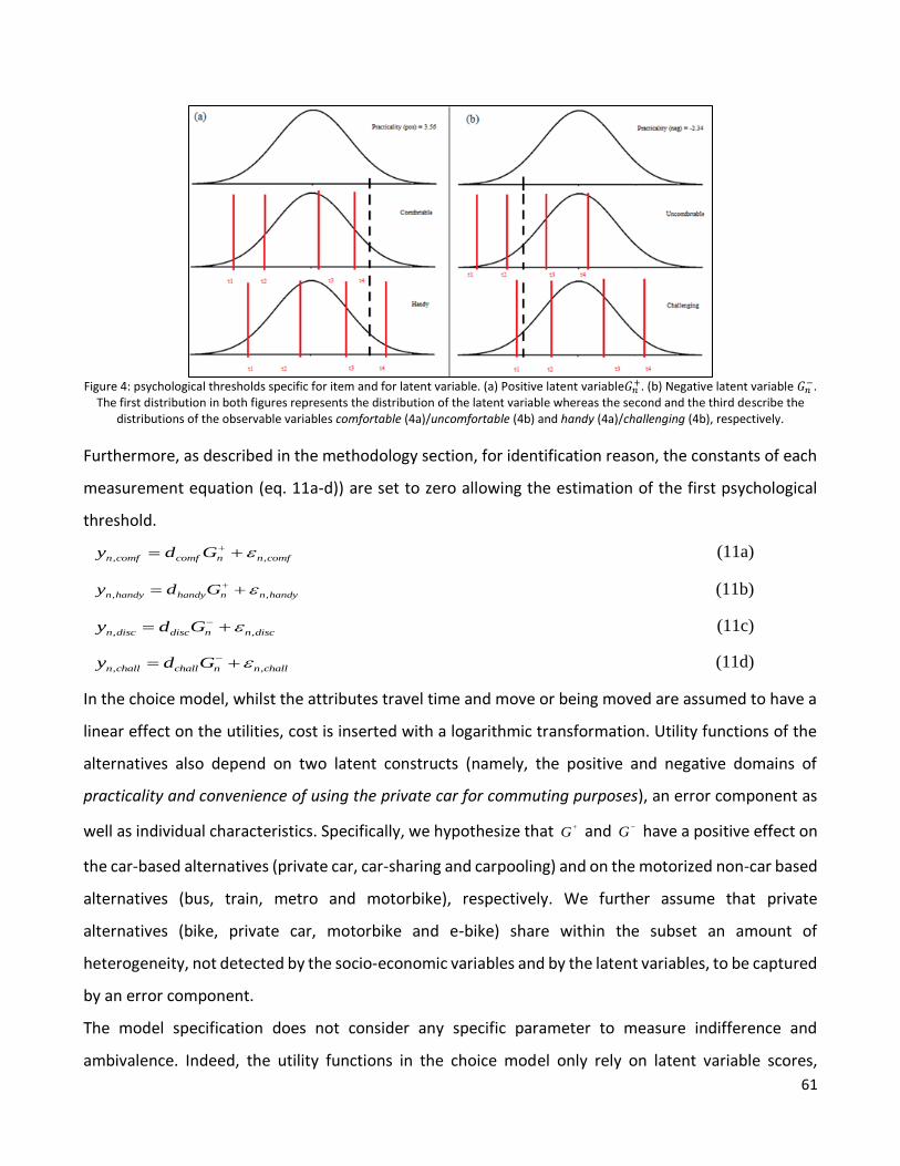
61

Figure 4: psychological thresholds specific for item and for latent variable. (a) Positive latent variable𝐺𝑛

+. (b) Negative latent variable 𝐺𝑛−.

The first distribution in both figures represents the distribution of the latent variable whereas the second and the third describe the distributions of the observable variables comfortable (4a)/uncomfortable (4b) and handy (4a)/challenging (4b), respectively.

Furthermore, as described in the methodology section, for identification reason, the constants of each

measurement equation (eq. 11a-d)) are set to zero allowing the estimation of the first psychological

threshold.

, ,n comf comf n n comfy d G (11a)

, ,n handy handy n n handyy d G (11b)

, ,n disc disc n n discy d G (11c)

, ,n chall chall n n chally d G (11d)

In the choice model, whilst the attributes travel time and move or being moved are assumed to have a

linear effect on the utilities, cost is inserted with a logarithmic transformation. Utility functions of the

alternatives also depend on two latent constructs (namely, the positive and negative domains of

practicality and convenience of using the private car for commuting purposes), an error component as

well as individual characteristics. Specifically, we hypothesize that G and G

have a positive effect on

the car-based alternatives (private car, car-sharing and carpooling) and on the motorized non-car based

alternatives (bus, train, metro and motorbike), respectively. We further assume that private

alternatives (bike, private car, motorbike and e-bike) share within the subset an amount of

heterogeneity, not detected by the socio-economic variables and by the latent variables, to be captured

by an error component.

The model specification does not consider any specific parameter to measure indifference and

ambivalence. Indeed, the utility functions in the choice model only rely on latent variable scores,

62

measuring the positive and the negative realms of practicality and convenience of using the private car

for commuting purposes. Probabilities of revealing an ambivalent or indifferent attitude are foreseen

using the results of the structural equation model.

The final model is estimated using Python-Biogeme version 2.4 (Bierlaire, 2016), using 10,000 Modified

Latin Hypercube Sample (MLHS) draws to approximate the integrals in Equations (5a) – (5b) – (6) (see

Hess et al., 2006).

2.6. Results

This section contains general results of the hybrid choice model and a focus on the preferences of

different categories of individuals, specifically those who are indifferent or ambivalent towards the

practicality and the convenience of commuting by a private car. Furthermore, we show how ambivalent

and indifferent subjects respond to changes in the attribute levels.

2.6.1. Structural model

Table 5 reports the coefficient estimates for the structural model. The latent variable practicality and

convenience of using the private car for commuting purposes is positively affected by number of days

of car use. It appears reasonable that individuals who use the car more often (either as a driver or

passenger) have a higher probability of considering the use of the private car for commuting purposes

practical and convenient. On the other hand, older individuals, those who are native Italian speakers,

French native speakers who do sport more often during the week and frequent car users who take

public means for commuting purposes, show a lower probability of assessing commuting by car

practical and convenient, all the rest being equal.

The number of days a private car is used also explains the latent variable unpracticality and

inconvenience, but in an opposite direction. That is, the more an individual uses a car, the lower the

probability of assessing commuting by car as inconvenient and unpractical, ceteris paribus. In addition,

this latent variable presents a lower value for students and for those who actually commute by a private

mean, whereas it has a higher value for those who have access to a private car in their household. This

latter result can be explained looking at the sample composition: only seventeen percent of

respondents do not have a car available in the household and, consequently, have never commuted by

private car. This segment likely idealizes the efficacy of commuting using this alternative,

63

underestimating the challenges and the inconveniences that individuals, who actually had the

opportunity of commuting by car, experience.

It is worth noting that, as hypothesized, the positive and the negative domains of the latent variable

measuring the ease of commuting by car are correlated: the parameter measuring the correlation ρ,

equals 0.575 and indicates a higher probability of observing individual assessments lying on the main

diagonal of the ESG. This finding empirically demonstrates the evaluative space model described by

Cacioppo and Bernston, since a high (low) value of the positive latent variable 𝐺+ is associated with a

high (low) value of the negative latent variable 𝐺−, proving that positive and negative feelings can be

experienced at the same time with strong intensities.

Structural model

Practicality and convenience of

commuting by car

Unpracticality and

inconvenience of commuting by

car

Par. (Rob. t-test) Par. (Rob. t-test)

Age -0.046 (-2.73) - -

Italian native speaker -0.381 (-2.98) - -

Number of days using the car (per week) 0.112 (6.48) -0.044 (-2.75)

French native speaker * Number of days doing sport -0.118 (-2.96) - -

Frequent car user * Main mode of transport (public) -0.212 (-2.30) - -

Car available to use - - 0.159 (1.76)

Student - - -0.184 (-1.89)

Main mode of transport privately owned - - -0.248 (-3.00)

Correlation parameter ρ 0.575 (9.02)

Table 5: coefficient estimates for the latent variables.

2.6.2. Measurement model

The latent variable 𝐺+ has a positive impact on both the observable items: the coefficients measuring

the effect of practicality and convenience of using the private car for commuting purposes on

comfortable and handy are 2.17 and 2.76, respectively (Table 6). The latent variable 𝐺− has a positive

impact on uncomfortable (1.92) and on challenging (2.55), even if for the latter the significance is

borderline (p-value = 0.09). In other words, an individual with a higher positive (negative) latent attitude

will be more likely to assess commuting by car highly comfortable and handy (uncomfortable and

challenging), all the rest being equal.

64

Psychological thresholds are statistically different within the same latent variable (that is τi,comf ≠ τi,handy,

for i = 1, … , 4) as well as between the two latent variables, indicating that the positive (negative) domain

of convenience and practicality of commuting by car affects differently the perception of observable

items comfortable and handy (uncomfortable and challenging).

Measurement model

Practicality and convenience of commuting by car Unpracticality and inconvenience of commuting by car


Comfortable Handy Uncomfortable Challenging

d 2.17 (3.53) 2.76 (2.63) 1.92 (2.44) 2.55 (1.69)


τ1 -6.95 (-3.67) -8.18 (-3.27) -2.54 (-3.38) -3.69 (-2.22)

τ2 -4.81 (-2.23) -5.62 (-1.85) -0.33 (-0.28) -1.07 (-0.42)

τ3 -3.15 (-8.35) -3.46 (-5.95) 1.48 (3.49) 1.56 (1.79)

τ4 -0.79 (-2.08) -0.19 (-0.27) 3.17 (7.94) 4.15 (4.79)

Table 6: coefficients estimates for the measurement model.

The structural equation model based on the evaluative space grids identifies four different categories

of respondents, according to the inclination pro/against and indifferent/ambivalent towards the

comfort and practicality of using the private car for commuting purposes. The model computes for any

individual the probabilities for all possible outcomes being observed, that are the probabilities of the

individual assessing commuting by car comfortable (from 1 to 5) and uncomfortable (from 1 to 5), as

well as handy and challenging, according to his own socio-economic characteristics and the thresholds

defined by the measurement model. The socio-demographic profiles and the resulting probabilities of

four different respondents are shown, as a matter of example, in Table 7 and Figure 5 respectively.

Individual 1

Indifferent

Individual 2

Ambivalent

Individual 3

Negative

Individual 4

Positive

Age 21 23 20 22

Native speaker Fre Ita Fre Ita

Number of days using the car (per week) 0 2 0 7

Number of days doing sport (per week) 3 3 3 1

Main mode of transport (private/public) Priv Pub Pub Priv

Table 7: Example of four different respondents

By using the ESG tool rather than a Likert scale, it becomes possible to correctly identify the probabilities

of an individual revealing any attitude, including indifference and ambivalence. Using 500 MLHS draws

65

to simulate the error terms of the model and following the partition suggested by Audrezet (2014)

shown in Figure 1, we compute the probability for each individual to exhibit a particular attitude

towards the convenience and the practicality of using the private car for commuting purposes, for both

ESG1 (measuring comfortable/uncomfortable) and ESG2 (measuring handy/challenging) (Figure 5).

Specifically, individual 1 displays the highest probability of considering commuting by car neither

comfortable/handy nor uncomfortable/challenging (bottom left corner probabilities equal to 0.989 and

0.992 for ESG1 and ESG2 respectively), whilst respondent 2 has the greatest probability of being classed

as being ambivalent towards commuting by car in both grids. Individual 3 has the highest probability of

considering commuting by car uncomfortable and challenging (i.e. 0.984 for ESG1 and 0.997 for ESG2),

whereas individual 4 has the highest probability of assessing the commuting by car comfortable and

handy.

Figure 5: Individual probabilities revealing 4 different attitudes. Probabilities accord to a scale red (low) to green (high). Corner values identify the probabilities of being classified negative (top-left), ambivalent (top-right), positive (bottom-right) and indifferent (bottom-

left) towards commuting by car.

66

2.6.3. Discrete choice model

The estimates of the choice model, which includes an error component in addition to the latent

variables, are shown in Table 8. The alternative specific constant parameters suggest that young Swiss

respondents prefer to commute by private car all the rest being equal. Following, carpooling, motorbike

and car-sharing are favored to public transport, bike, e-bike and moving walkway, revealing a

pronounced inclination for car-based alternatives, all rest being equal. The walking distance (move or

being moved attribute) has a negative impact on all the alternatives, so have the travel time and the

log(monthly cost), ceteris paribus. Respondents are willing to pay 6 CHF more per month, based on an

expense of 15 CHF per month (average monthly cost of bike and e-bike), for saving about five percent

of the commuting time per day (that is saving about 45 minutes per month). The willingness to pay per

month for saving five percent of the commuting time per day for PT, PC, CS, CP and MO is 46 CHF, based

on an expense of 150 CHF per month (average monthly cost of the alternatives listed above).

Hypothetical low (different for cities, on average about 6500 CHF/month) and medium wages (on

average about 8800 CHF/month) have a positive impact on non-car-based alternatives, or otherwise

stated, having a high wage increases the probability of commuting by PC, CS and CP, which are the most

expensive alternatives in the experiment.

The estimates of the socio-economic variables indicate that individuals who commute by a private

mean have a higher probability of choosing a private mean for the hypothetical commute trip too,

whilst those who conduct an active life, doing sport two or more times per week, are more likely to

choose an active transportation mean (i.e. bike, e-bike or moving walkway), all the rest being equal.

The cultural background of an individual affects the mode choice for commuting: German native

speakers display a higher probability of choosing public transport, bike, e-bike and moving walkway,

and similarly Italian native speakers prefer non-car-based alternatives. However, the impact of the

dummy variable indicating an Italian cultural background is much lower than the one representing a

German cultural background. Gender has a significant effect on the utility of carpooling and in detail,

male respondents have a lower probability of considering carpooling an appealing alternative. This

finding can be due to a higher attention of females for environmental issues (see among others

Patterson et al., 2005; Bolduc et al., 2008). Inter-alternative correlation exists within the set of private

alternatives and it is captured by the error component, meaning that these alternatives share common

heterogeneity not detected by the socio-economic variables.

67

The latent variable measuring the positive domain of convenience and practicality of using the private

car for commuting purposes, 𝐺+, has a positive effect (3.28) on the utility functions of the car-based

alternatives (PC, CS, CP) in the choice model, suggesting that individuals who have a positive attitude

towards the convenience of the private car use for commuting trips show a higher probability of

choosing private car, car-sharing and carpooling than those who have a neutral or negative attitude,

ceteris paribus. Conversely, the latent variable measuring the negative domain 𝐺− has a positive impact

(2.79) on the utility functions of PT and MO, suggesting that subjects who consider commuting by car

challenging and uncomfortable have a higher probability of choosing public transport (train, bus, metro)

and motorbike than those who have a less negative attitude, all the rest being equal.

68

Choice model

Alternative specific constants Par. (Rob. t-test) Alternative specifications

Public Transport (PT) -4.92 (-3.74)

Bike (BI) -9.03 (-4.58)

Moving Walkway (MW) -8.24 (-4.33)

Private Car (PC) - -

Car-sharing (CS) -4.13 (-8.72)

Carpooling (CP) -2.96 (-5.15)

Motorbike (MO) -3.93 (-2.84)

Electric bike (EB) -6.29 (-3.04)

Attributes

Log(monthly cost) -0.564 (-2.18) PT, PC, CS, CP, MO

Log(monthly cost) -0.433 (-2.13) BI, EB

Travel time -0.173 (-14.71) PT, PC, CS, CP, MO

Travel time -0.177 (-9.31) BI, EB

Move or being moved -1.43 (-11.13)

Low Wage 2.60 (11.96) PT, BI, MW, MO, EB

Medium Wage 1.03 (6.21) PT, BI, MW, MO, EB

Socio-economic characteristics

Actual mode for commuting (private) 0.943 (3.15) BI, PC, MO, EB

Italian native speaker -0.804 (-1.71) PC, CS, CP

German native speaker 2.47 (2.81) PT, BI, MW, EB

Sportsman 0.703 (2.33) BI, MW, EB

Male -0.858 (-1.78) CP

Error components

Private means -2.60 (-15.38) BI, PC, MO, EB

Latent variables

G 3.28 (14.19) PC, CS, CP

G 2.79 (13.88) PT, MO

Table 8: estimates of the choice model. The last column contains the alternatives whose utilities depend on the corresponding parameter (for instance, the parameter measuring Low Wage is included in PT, BI, MW, MO and EB utility functions). If the cell is blank,

the parameter is included in the whole set of alternatives.

2.6.4. Effect of latent variables

The combined effect of positive and negative attitudes towards the convenience and the practicality of

using the private car for commuting purposes is observed assigning respondents to four different

categories (i.e. positive, negative, indifferent and ambivalent), according to simulated individual scores.

In detail, we first compute the latent variable scores according to the structural model specification and

then, using the specific sets of psychological thresholds estimated for the different grids, we can

69

allocate any respondent to a different category for any grid. As an example, let us consider a subject

whose scores on the latent variables 𝐺+ and 𝐺− are -5 and 3.5 respectively. According to the

psychological thresholds of the grid comfortable vs uncomfortable, this subject has a high probability

of selecting the cell (2:5) in the ESG1, revealing a high propensity for judging commuting by car

uncomfortable (negative attitude). However, the same subject exhibits an ambivalent attitude towards

the dichotomy handy/challenging having a high probability of selecting the cell (3:4) in the ESG2. One

of the main strength of the evaluative space grid is its ability to distinguish subjects who are torn

between a positive and a negative attitude, and who can be therefore either ambivalent or indifferent.

Indeed, the tool proposed by Likert to measure attitudes fails in distinguishing these categories, which

are merged together on the neutral point of the scale.

We calculate and use market shares for the eight alternatives using 500 MLHS draws to simulate the

error components for testing the hypothesis that individuals with an indifferent attitude have different

preferences of those who have an ambivalent attitude (a table containing market shares is available

upon request). Guaranteed that individuals who consider commuting by private car convenient and

practical have different preferences from those who consider it inconvenient and unpractical, we then

compare market shares for indifferent and ambivalent categories using Welch’s t-tests. Table 9 displays

the test outcomes: a key finding is that thirteen out of sixteen t-tests reject the null hypothesis of

equality (with a p-value < 0.1), suggesting that individuals who have an ambivalent attitude towards

the convenience and the practicality given by the usage of the private car for commuting purposes

reveal different preferences for the mode choice in a commuting trip than those who exhibit an

indifferent attitude.

PT BI MW PC CS CP MO EB

ESG1 Rej 0.01 Rej 0.1 Rej 0.05 Rej 0.01 Rej 0.01 Rej 0.01 Acc Rej 0.05

ESG2 Rej 0.01 Rej 0.05 Acc Rej 0.01 Rej 0.01 Rej 0.01 Acc Rej 0.01

Table 9: Welch’s t-tests Ambivalent vs Indifferent market shares. Null hypothesis: equal market shares. “Rej 0.01 (0.1)” = reject the null hypothesis (p-value < 0.01 (0.1)); “Do not Rej” = cannot reject the null hypothesis (p-value > 0.1).

70

INCREASE IN TRAVEL TIME BY 10%

PT BI PC

GRID 2 GRID 3 GRID 2 GRID 3 GRID 2 GRID 3

amb ind amb ind amb ind amb ind amb ind amb ind mean -1.35 -2.25 -1.59 -2.43 -1.95 -0.22 -1.82 -0.01 -1.16 -2.20 -1.03 -2.06

var 0.63 0.27 0.68 0.07 0.61 0.21 0.61 0.00 0.62 0.19 0.60 0.12

p-value 0.000 0.031 0.004 0.000 0.000 0.033

INCREASE IN MONTHLY COST BY 10%

PT BI PC

GRID 2 GRID 3 GRID 2 GRID 3 GRID 2 GRID 3

amb ind amb ind amb ind amb ind amb ind amb ind mean -0.92 -1.64 -1.11 -1.82 -0.67 -0.06 -0.63 0.00 -1.21 -2.68 -1.08 -2.67

var 0.37 0.17 0.39 0.03 0.02 0.01 0.03 0.00 0.66 0.00 0.65 0.00

p-value 0.001 0.025 0.002 0.000 0.000 0.000

INCREASE IN MOVE OR BEING MOVED BY 10%

PT BI PC

GRID 2 GRID 3

This alternative has DST = 0

GRID 2 GRID 3

amb ind amb ind amb ind amb ind mean -0.56 -0.95 -0.64 -1.03 -0.40 -0.65 -0.49 -1.25

var 0.14 0.05 0.14 0.03 0.12 0.04 0.15 0.06

p-value 0.044 0.040 0.064 0.028

Table 10: elasticities for market shares and travel time (top table), market shares and cost (mid table), market shares and density (bottom table). The bold values, reported in the last row of any table, represent the p-values computed for a Welch’s t-test. Null

hypothesis: equal elasticities between ambivalent and indifferent categories.

A further important finding is that individuals who have an ambivalent attitude towards the practicality

and convenience of using the private car for commuting purposes react differently to a change in the

attribute levels than those who possess an indifferent attitude. Indeed, after calibrating the model, we

measure the responsiveness of the market shares to a change in travel time, cost and move or being

moved for the different alternatives. For brevity, we only show here the elasticities for public transport,

bike and private car, which are the most used transportation means within the four categories. Upon

request, authors the elasticities for all categories and change in attribute levels can be provided.

Evidence shows that indifferent individuals respond more actively to a change in travel time, cost and

density (i.e. move or being moved) for public transport and private car than ambivalent subjects, whilst

the latter category of persons displays a larger elasticity for bike. Table 10 shows that a 10 percent

increase in travel time for public transport reduce the market share of 1.35 percent or 1.59 percent

(according to ESG1 and ESG2 categorizations) and 2.25 percent or 2.43 percent for ambivalent and

indifferent subjects respectively. A similar pattern is displayed for a 10 percent increase in travel time

for private car, whilst for bike, the market shares are reduced more for the ambivalent category (1.95

and 1.82 percent according to ESG1 and ESG2 classifications) than for the indifferent category (0.22

71

percent according to ESG1 and 0.01 percent according to ESG2). An analogous scheme is reported for

a 10 percent increase in cost and density. The null hypothesis stating that individuals having an

ambivalent attitude display the same elasticity of those having an indifferent attitude is rejected in all

the tests.

Summarizing, the results contained in this section confirm the hypothesis that individuals possessing

an ambivalent or indifferent attitude have different preferences and different behaviors. Tests on the

differences in market shares and elasticities are consistent with the findings of previous works

suggesting that distinguishing individuals with an ambivalent and indifferent attitude is as important as

identifying those with a positive and negative inclination as they tend to act differently.

2.7. Discussion and conclusions

The definition of attitudes in transportation literature presents substantial differences according to the

type of study. Psychologists use numerous measurable variables having a different valence (from

extreme negative to extreme positive) to shape an attitude, whilst researchers who mainly focus on the

consequent behavior of the attitudes employ a limited number of items, with either an extreme positive

or negative valence. In several applications in choice modelling the randomness of the latent variable

(attitude) is increased because of the use of a reduced set of items, entailing a less precise definition of

the attitude itself and a poor representation of individuals on the latent continuum. In some studies,

attitudes are inserted in the discrete choice experiment as an attribute and are measured using a

qualitative ordered scale (low – medium – high). Such a misspecification of the latent construct entails

an even larger randomness of the attitude (for instance, respondents can identify with “comfort” the

quality of the seats, the presence of air conditioning, the space for standing and several more

observable variables).

The Likert scale, which is the gold standard tool for measuring the observable variables in

transportation, is appropriate for distinguishing subjects with a positive or negative valence, but it is

not suitable for disentangling persons with indifferent and ambivalent inclinations, who lie both on the

neutral point of the latent continuum (central values of the scale). The Evaluative Space Grid, proposed

by Larsen et al., is a single-item measure of positivity and negativity following the theoretical framework

of Evaluative Space Model, stating that positive and negative feelings can be experienced at the same

time, also with strong intensities. The ESG is purposely designed to differentiate between ambivalence

72

and indifference, as well as positive and negative attitudes. The differentiation between subjects having

an ambivalent and indifferent attitude, which cannot be realized with a Likert scale, can provide further

insights to policy makers, who can study ad hoc policies on different segments of the population. As a

matter of fact, it has already been shown, in contexts such as politic elections and environmental

behavior (Costarelli and Colloca, 2004; Yoo, 2010; Thornton, 2011), that indifferent and ambivalent

individuals act differently.

This work proposes a methodology to include the ESG in the framework of hybrid choice models: the

grids are modelled, in the structural equations, by means of two latent variables, representing positive

and negative domains respectively, and, in the measurement equations, two ordered logit regressions

link the observables items to the latent variables. It is worth noting that the hybrid choice model does

not include specific parameters to measure a direct effect of indifference and ambivalence on the

alternatives. The lack of these parameters could suggest the use of common items measured with a

Likert scale. However, even if the econometrics behind the construction of latent variables is the same,

using the evaluative space grid tool preserves the correct collection of data aimed at measuring the

ambivalence and indifference, which could bring to biased results if sequentially structured conversely

framed questions are used. A possible follow-up of this research is the introduction of specific

parameters in the hybrid choice model measuring the effect of indifference and ambivalence, using a

categorical method for defining the four different types of attitudes.

In addition to the methodological contribution, this work tests the hypothesis that indifferent and

ambivalent individuals display different preferences in a context of transportation mode choice for

commuting trips and therefore the distinction of such categories becomes of primary importance for

policy motives. In particular, we show that subjects who consider commuting by private car

comfortable/handy and uncomfortable/challenging at the same time (ambivalent individuals) reveal

different preferences from those who judge commuting by private car neither comfortable/handy nor

uncomfortable/challenging (indifferent individuals), for 7 out of 8 alternatives of transport.

Furthermore, these categories also respond differently if the proposed alternatives experience a

change in cost, travel time or density of the transportation system. Specifically, the elasticity is larger

for individuals with an indifferent attitude when travel time, cost and density for public transport and

private car increase, whilst subjects having an ambivalent attitude display a larger elasticity when

similar changes occur for bike.

73

The inclusion of attitudes in studies modeling individuals’ preferences obtained great appreciation

because of possible implications for policy purposes. Indeed, specific campaign for individuals who

have, for instance, a strong inclination towards environmental concerns or attachment to the car can

be adopted. This work moves one step forward, claiming that it is important to consider also the

segment of individuals having a neutral inclination, that is subjects revealing an ambivalent or

indifferent attitude. Once the composition of these clusters has been identified, it is possible to draw

even more powerful and effective policies.

74

References

Abou-Zeid, M., Ben-Akiva, M., 2011. The effect of social comparisons on commute well-being. Transport Policy 19, 93–104.

Abrahamse, W., Steg, L., Gifford, R., Vlek, C., 2009. Factors influencing car use for commuting and the intention to reduce

it: a question of self-interest or morality? Transportation Research Part F 12, 317–324.

Anable, J., 2005. ‘Complacent Car Addicts’ or ‘Aspiring Environmentalists’? Identifying travel behaviour segments using

attitude theory. Transport Policy 12, 65 – 78.

Atasoy, B., Glerum, A., Bierlaire, M., 2012. Attitudes towards mode choice in Switzerland. Report TRANSP-OR 110502.

Transport and Mobility Laboratory, EPFL.





Bahamonde-Birke, F. J., Hanappi, T., 2016. The potential of electromobility in Austria: Evidence from hybrid choice models

under the presence of unreported information. Transportation Research Part A 83, 30-41.

Ben-Akiva, M., Walker, J., Bernardino, A.T., Gopinath, D.A., Morikawa, T., Polydoropoulou, A., 1999. Integration of Choice

and Latent variable Models. Massachusetts Institute of Technology, Cambridge.

Bierlaire, M., 2016. PythonBiogeme: a short introduction, Technical report TRANSP-OR 160706. Transport and Mobility

Laboratory, ENAC, EPFL. Retrieved from: http://biogeme.epfl.ch/documentation/pythonfirstmodel.pdf

Bolduc, D., Daziano, R., 2010. On estimation of hybrid choice models. In book: Choice Modelling: the state-of-art and the

state-of-practice, Publisher: Emerald, Editors: S. Hess and A. Daly, 259 -287.

Bolduc, D., Boucher, N., Daziano, R., 2008. Hybrid Choice Modeling of New Technologies for Car Use in Canada. Journal of

the Transportation Research Board 2082, Transportation Research Board of the National Academies

Bolduc, D., Ben-Akiva, M., Walker, J.L., Michaud, A., 2005. Hybrid Choice Models with Logit Kernel: Applicability to Large

Scale Models, in M.E.H. Lee-Gosselin and S.T. Doherty, eds. Integrated Land-Use and Transportation Models:

Behavioral Foundations, Emerald Group Publishing, 275-302.



2909.115.3.401



Daly, A., Hess, S., Patruni, B., Potoglou, D., Rohr, C., 2012. Using ordered attitudinal indicators in a latent variable choice

model: a study of the impact of security on rail travel behavior. Transportation 39, 267 – 297. DOI:10.1007/s11116-

011-9351-z

Daziano, R., Bolduc, D., 2013. Incorporating pro-environmental preferences toward green automobile technologies through

a Bayesian Hybrid Choice Model. Transportmetrica 9(1), 74 – 106.

75

Domarchi, C., Tudela, A., Gonzalez, A., 2008. Effect of attitudes, habit and affective appraisal on mode choice: an application

to university workers. Transportation 35, 585–599. DOI 10.1007/s11116-008-9168-6

Espino, R., De Dios Ortuzar, J., Roman, C., 2003. Analysing the effect of latent variables on willingness to pay in mode choice

model. Association for European transport.

Espino, R., De Dios Ortuzar, J., Roman, C., 2006. Analysing demand for suburban trips: A mixed RP/SP model with latent

variables and interaction effects. Transportation 33, 241 – 261. DOI 10.1007/s11116-005-2299-0

Habib, K. M. N., Kattan, L., Islam, M. T., 2011. Model of personal attitudes towards transit service quality. J. Adv. Transp. 45,

271–285.

Hess, S., Shires, J., Jopson, A., 2013. Accommodating underlying pro-environmental attitudes in a rail travel context:

Application of a latent variable latent class specification. Transportation Research Part D 25, 42–48.

Hess, S., Train, K. and Polak, J., 2006. On the use of modified latin hypercube sampling (MLHS) method in the estimation of

mixed logit model for vehicle choice, Transportation Research Part B 40(2), 147–163. doi: 10.1016/j.trb.2004.10.005

Johansson, M. V., Heldt, T., Johansson, P., 2006. The effects of attitudes and personality traits on mode choice.

Transportation Research Part A 40, 507–525.



Khattak, A., Wang, X., Son, S., Agnello, P., 2011. University student travel in Virginia: is it different from the general

population? Transportation Research Record 2255, 137 – 145.



Likert, R., 1932. A technique for the measurement of attitudes. Archives of Psychology, R. S. Woodworth Editor, 140, New

York.

Mikrozensus Mobilität und Verkehr, 2010. Bundesamt für Statistik: https://www.bfs.admin.ch/bfs/de/home.html

Mokhtarian, L.P., Salomon, I., Redmond, L.S., 2001. Understanding the demand for travel: it’s not purely ‘derived’.

Innovation 14(4), 355 – 380.

Ngene 1.1.2 User Manual & Reference Guide, 2014. http://www.choice-metrics.com/download.html

Ory, D.T., Mokhtarian, P.L., 2005. When is getting there half the fun? Modeling the liking for travel. Transportation Research

Part A 39, 97–123.

Patterson, Z., Haider, M., Ewing, G., 2005. A gender-based analysis of work trip mode choice of suburban Montreal

commuters using stated preference data. Transportation Research Record: Journal of the Transportation Research

Board 1924, 85 – 93. doi: 10.3141/1924-11.

Prillwitz, J., Barr, S., 2011. Moving towards sustainability? Mobility styles, attitudes and individual travel behavior. Journal

of Transport Geography 19, 1590–1600.

http://dx.doi.org/10.1037/h0032590

76

Raveau, S., Daziano, R., Yanez, M.F., Bolduc, D., de Dios Ortuzar, J., 2010. Sequential and simultaneious estimation of hybrid

discrete choice models: Some new findings. Transportation Research Record Journal of the Transportation Research

Board 2156(1), 131 – 139.

Rose, J.M., Bliemer, M.C.J., 2008. Stated preference experimental design strategies, in Hensher, D.A. and Button, K.J. (eds.)

Handbook of Transport Modelling, Elsevier, Oxford, Ch. 8, 151-180.

Rose, J.M., Bliemer, M.C.J., Hensher, D.A., Collins, A.C., 2008. Designing efficient stated choice experiments involving

respondent based reference alternatives. Transportation Research Part B 42(4), 395-406.

Rundmo, T., Nordfjærn, T., Iversen, H. H., Oltedal, S., Jørgensen, S. H., 2011. The role of risk perception and other risk-related

judgements in transportation mode use. Safety Science 49, 226–235.

Shiftan, Y., Barlach, Y., Shefer, D., 2015. Measuring passenger loyalty to public transport modes. Journal of Public

Transportation 18(1).

Tay, L., Kuykendall L., 2017. Why self-reports of happiness and sadness may not necessarily contradict bipolarity: a

psychometric review and proposal. Emotion Review 9(2), 146-154. doi: 10.1177/1754073916637656.



Thurstone, L.L., 1928. Attitudes can be measured. American Journal of Sociology 33, 529 – 554.

Thurstone, L.L., Chave, E.J., 1929. The measurement of attitude. Chicago: University of Chicago Press.

Whalen, K.E., Páez, A., Carrasco, J.A., 2013. Mode choice of university students commuting to school and the role of active

travel. Journal of Transport Geography 31, 132 – 142.


72(1), 163-177. doi: 10.1017/S0022381609990545

77

Chapter 3. Generalized versus localized attitudinal responses in discrete choice

Antonio Borriello1, John M. Rose2

1Università della Svizzera italiana, 2University of Technology of Sydney

Abstract

In his theory of planned behavior, the psychologist Ajzen illustrates that psychological

factors are precursor of behavior. Following this theoretical framework, in the last

decades many researchers explored the importance of attitudes and perceptions in

determining choice behavior in a transportation setting. A more recent debate within

the psychological literature concerns the stability of attitudes. The first school of

thought argues that attitudes embody long-term stable constructs which are

“memory-based” (generalized attitudes), and it contrasts the idea that attitudes are

short-term situational specific concepts, constructed at the time a specific situation

occurs (localized attitudes). A mediating classification of attitudes consists in defining

attitudes as created via a mixture of both short and long-term influences.

The current practice when modeling individual choices consists in employing only

generalized attitudes. This paper examines the stability of attitudes within a stated

choice experiment framework and shows the importance of including localized

attitudes when modeling preferences.

Subjects are asked to provide responses to the same attitudinal questions, both prior

to undertaking the choice experiment, and after each stated choice task they

complete as part of the survey. Evidence shows that generalized and localized

attitudes diverge for most of the respondents and their impact on individual choices

is substantial. Additionally, considering generalized and localized attitudes separately,

only captures partial information related to the psychological process leading to the

choice. Finally, the omission of localized attitudes may potentially lead to inconsistent

estimates as is the case of the willingness to pay.

Keywords: stability of attitudes, individual preferences, willingness to pay

78

3.1. Introduction

Over the past four decades, discrete choice models (DCM) have become the dominant method for

modelling and understanding traveler preferences and behavior. Estimation of DCMs requires analysts

to specify separate utility functions for the different alternatives present within a given market of

interest. Typically, these utility functions are defined in terms of the attributes of the alternatives being

examined, the characteristics of the decision makers, or some combination of the two. By observing

how variations in the attributes of the alternatives or characteristics of the decision makers

systematically vary with the observed choices within the market, the influence on choice behavior of

each attribute describing the alternatives and/or characteristic of the individual decision makers can be

determined in the form of utility weights. Based on the overall combined utility values derived for each

alternative within the model, the probability that each alternative will be chosen is then calculated,

which subsequently provides a direct mapping between the individual specific choice environment

described within the data and overall market behavior.

Despite being somewhat less used in practice, early theorists identified the importance that the

attitudes and perceptions held by different decision makers towards both the objects being considered,

and towards more general life concerns, can play on choice behavior. For example, McFadden (1980),

based on theories of consumer behavior, discussed the importance of including attitudinal data within

the DCM framework, stating “The theory of the economically rational utility-maximizing consumer,

interpreted broadly to admit the effects of perception, state of mind, and imperfect discrimination,

provides a plausible, logically unified foundation for the development of models of various aspects of

market behavior.” Currim (1981) and Swait (1994) demonstrated how generalized attitudes and

perceptions can be used to build models with segmented preferences resulting in improved forecasting

and model fits for both stated preference and revealed preference data sets. Citing even earlier work

on hybrid conjoint models (e.g., Green et al. 1981 and Green 1984) as his inspiration, McFadden (1986)

derived the theoretical framework for the hybrid choice model (HCM) allowing for the inclusion of both

generalized attitudes and alternative specific perceptions, to enter the utility functions of a DCM via a

latent variable structure. The model was first operationalized by Train et al. (1987) to explore the impact

of attitudes upon rate scheduling for public utilities, whilst Swait (1994) used a similar modelling

structure to model preferences for different beauty products. Similar conceptual frameworks were

79

made operational using various transportation contexts by Morikawa (1989), Morikawa et al. (1990),

Hensher (1990), Ben-Akiva and Morikawa (1990), Vieira (1992) and Ben-Akiva and Boccara (1993).

Of late, the inclusion of attitudinal and perceptual data within DCMs has become increasingly popular

with a spate of recent papers examining how attitudes and perceptions influence bicycle choice (e.g.,

Maldonado-Hinarejos et al. 2014), the relationship between mode choice and the built environment

(e.g., Van Acker et al. 2011), and automobile choice (e.g., Daziano and Bolduc 2013a). Other recent

papers have explored methodological issues related to how best to incorporate attitudes and

perceptions within the DCM framework (e.g., Ben-Akiva et al., 2002; Daziano and Bolduc, 2013b;

Raveau et al., 2012; Vij and Walker, 2016). More recently, Bahamonde-Birke et al. (2017) have argued

that there exists a difference between attitudes and perceptions, where attitudes are defined as “a

mindset or a tendency to act in a particular way due to both an individual’s experience and

temperament” (Allport, 1935), whereas perceptions represent the organization, identification and

interpretation of sensory information aiming at representing and understanding the environment

(Schacter et al., 2011). In spite of the earlier cited work which explicitly discussed the different role that

generalized attitudes and perceptions have on choice, Bahamonde-Birke et al. (2017) argue that

previous work has tended to ignore this distinction treating the two concepts interchangeably.

Thus, despite recent attention, the idea that attitudes and perceptions play a significant role in choice

behavior is not new. The focus of the current paper is to examine the stability of attitudes within a

stated choice experiment framework. As such, we do not seek to explore explicitly the role of

perceptions, which as discussed above, has been shown to play an important role in describing choice

behavior. Our interest in the temporal stability of attitudes stems from an ongoing debate within the

psychological literature where there appear to exist three different schools of thought as to whether

or not attitudes are largely fixed or somewhat transient. The first school of thought identified assumes

that attitudes are long term stable constructs which are “memory-based” such that an attitude towards

an object is linked to one or more global evaluations that brought to the mind once the object is

encountered. This has led for example to the development of the MODE (in case of one evaluation,

Fazio, 1990) and MCM (in case of more than one evaluations, Petty et al., 2007) attitudinal model

frameworks. The second school of thought related to the temporal stability of attitudes is to assume

that attitudes are short term situational specific constructs that are developed “on the spot”. For

example, Gawronski’ and Bodenhausen (2007) propose what they call the APE model which assumes

80

that associative and propositional processes linked to attitude formation are sensitive to contextual

influences. Similarly, Schwarz (2007) and Conrey’ and Smith (2007) propose what have been termed

connectionist models for attitude formation. These connectionist models posit that attitudes are

constructed at the time a specific situation occurs and that evaluative judgments are formed only when

required rather than being stored in longer term memory. The third school of thought on attitude

formation assumes that attitudes are created via a mixture of both short and long-term influences. This

intermediate view of attitude formation, represented by models such as the IR model (Cunningham and

Zelazo, 2007; Cunningham et al., 2007), assume that evaluative processes towards objects are part of

an iterative cycle where the current evaluation of a stimuli can be adjusted as new contextual and

motivational information arises, and that adjustments to attitudes occurs in an iterative manner over

time resulting in an updated evaluation according to the specific stimuli and context faced. Through

this work we refer to long term stable attitudes as generalized, whilst short term situational specific

constructs are labelled localized. We refer the interested reader to Bohner and Dickel (2011) or Crano

and Prislin (2006) for further discussions related to the debate on the temporal nature of attitude

formation.

Understanding the temporal stability of attitudes is critical to transportation planning and research

given the link between attitudes and behavior as explained by the theory of planned behavior (Ajzen,

1985) which has become the dominant theoretical framework adopted within the literature. This is

because, if attitudes are a precursor towards action, one mechanism to change travel behavior may be

via the ability of transport planners to change attitudes. The classical models of attitude change, such

as the elaboration likelihood model (Petty and Wegener, 1999), or the heuristic/systematic model

(Chen and Chaiken, 1999), rely on the introduction of new stimuli, such as a message or advertisement,

which when processed by the individual, can result in an attitude change alongside a change in

behavior. Such theories are used in part to motivate travel behavior change programs, such as

TravelSmart (Red3, 2005).

The current chapter reports the results of a stated choice experiment where respondents are asked to

provide responses to the same attitudinal question, both prior to undertaking the choice experiment,

and after each stated choice task they complete as part of the survey. The approach adopted allows for

an examination as to how attitudinal responses vary as the attribute levels of the alternatives presented

within the experiment change over repeated choice tasks. The survey approach allows for an

81

examination of the path dependence of attitudinal changes within a stated choice framework, as well

as an investigation as to how previously stated attitudes can affect current decisions.

The remainder of the paper is organized as follows. In the next section we briefly introduce the

methodology and then present case study, focusing on the structure of the survey and the sample used

for the analysis. The following sections contain the specification of the model used to analyze the data

and a discussion of the results. Finally, we conclude the paper summarizing the main findings and the

benefit of considering psychological aspects constructed in the situation based on currently accessible

information, as well as general attitudes pre-stored in memory.

3.2. Theoretical background

An overview of the general framework of hybrid discrete choice model is presented in this section (see

Walker, 2001; Ben-Akiva et al., 2002; Daly et al., 2012 for a more detailed explanation of the

methodology). A HDCM consists of a simultaneous estimation of two distinct processes, a structural

equation model and a discrete choice model. Whilst the former explores and defines the structure of

the psychological factors using two types of relationships (structural and measurement equations), the

latter determines individuals’ preferences.

Let consider n respondents who face a choice set composed by J alternatives and let assume that the

decision makers are rational, choosing the alternative that maximizes the personal utility. The chosen

alternatives is

1argmax(( ( , , , ; , , , ) | 1,..., ; 1,..., )n nj j n j n njk U f X W Y G a d c n N j J (1)

where jX is a vector of attributes for alternative J, n

W represents a vector of socio-economic variables

describing individual n, n

G indicates the vector of l latent variables, whilst the matrix jY defines which

latent variables are inserted in the utility function of alternative J. The impacts of these latent variables

are measured by the vector c, whilst vectors a and d represent the impact that attributes and

socioeconomic variables have on the utility of the alternative respectively. The error term nj is i.i.d.

extreme value type 1. The analyst can define the function 1( )f g according to the data.

A latent variable is defined in the structural equation as a function of observable data (such as individual

characteristics and alternative features) plus a stochastic component ( nl ) which is typically assumed

to be Normal distributed with zero mean and a certain covariance matrix:

82

nl nl jl nlG bW pX (2)

The attitudinal response niy for the ith indicator variable (or item) is a (categorical) variable modelled

by a measurement equation. Its general formulation is

ni i i n niy d G (3)

where i

is a constant, the vector id measures the effect of the latent variable on the attitudinal

response (note that this vector may contains zero values if the latent variables do not have an impact

on a given item) and ni is an error term. According to its specification, the type of measurement model

is determined (for example ordered logit or ordered probit).

The objective of the analyst is to estimate the parameters included in the three types of relationships.

To do so, it is necessary to maximize the likelihood of jointly observing the vector of choices and

indicators k and y. The parameters of interest are then estimated using technique of simulated

maximum likelihood, employing random draws to describe the probability distributions associated with

the latent variables.

It is worth noting that the methodology used for defining the measurement equations in this work

slightly differs from the standard practice because the attitudinal indicators are collected by means of

the ESG instrument. The reader can refer to the previous chapter of this thesis for a detailed explanation

of the method.

3.3. Case study

3.3.1. The survey

The ad hoc experiment set up for this paper allows us to explore the role that different types of attitudes

play in explaining the decision-making process in transportation. Differently from the common HDCM

practice that only employs attitudes stored in memory, we hypothesize that attitudes can change

according to the situation and therefore the researcher should consider such divergences when

modelling the travel demand.

The questionnaire consists of four parts. In the first section, the overall opinion on trains is collected

through indicators measuring the overall satisfaction/dissatisfaction (Figure 1). Such indicators

represent the manifestation of generalized attitudes and are function of socio-economic variables. The

instrument used to collect attitudes is the evaluative space grid (ESG) proposed by Larsen et al. (2009).

83

A grid can replace a set of indicators measured with a semantic differential scale without any loss of

information and it is suitable for collecting either a specific or a general attitude, affecting notably on

the length of our survey. In the next section, we describe such an instrument more appropriately.

Figure 1: Evaluative space grid for measuring the general satisfaction/dissatisfaction towards trains.

In the second section, respondents are asked to describe their last trip taken by train defining, among

other characteristics, access time, waiting time, travel time, transfer time, egress time, fare, crowd on

the platform, seat availability and temperature in the train. In addition, the localized

satisfaction/dissatisfaction towards this trip is collected using a further ESG. In the next section,

interviewees are expected to assess their satisfaction/dissatisfaction for six alternative train services,

pivoted around the one they recently took (Figure 2). The expected attitude of a hypothetical offer,

being constructed on the spot, represents a localized attitude.

84

Figure 2: Example of a hypothetical train service and ESG related to it.

Following, the hypothetical train services pivoted around the actual are used in a stated preference

experiment consisting in six choice tasks with two alternatives. Respondents are asked to choose

between the same train service he/she described in section two (reference alterative) and the

hypothetical train service (stated alternatives) for taking the exactly same trip they described. Figure 3

displays a screen capture representing an example of choice task. The software Ngene 1.1.2 (Ngene,

2014) is used to maximize the D-efficiency for a pivotal design (Rose et al., 2008; Rose and Bliemer,

2008) with four blocks.

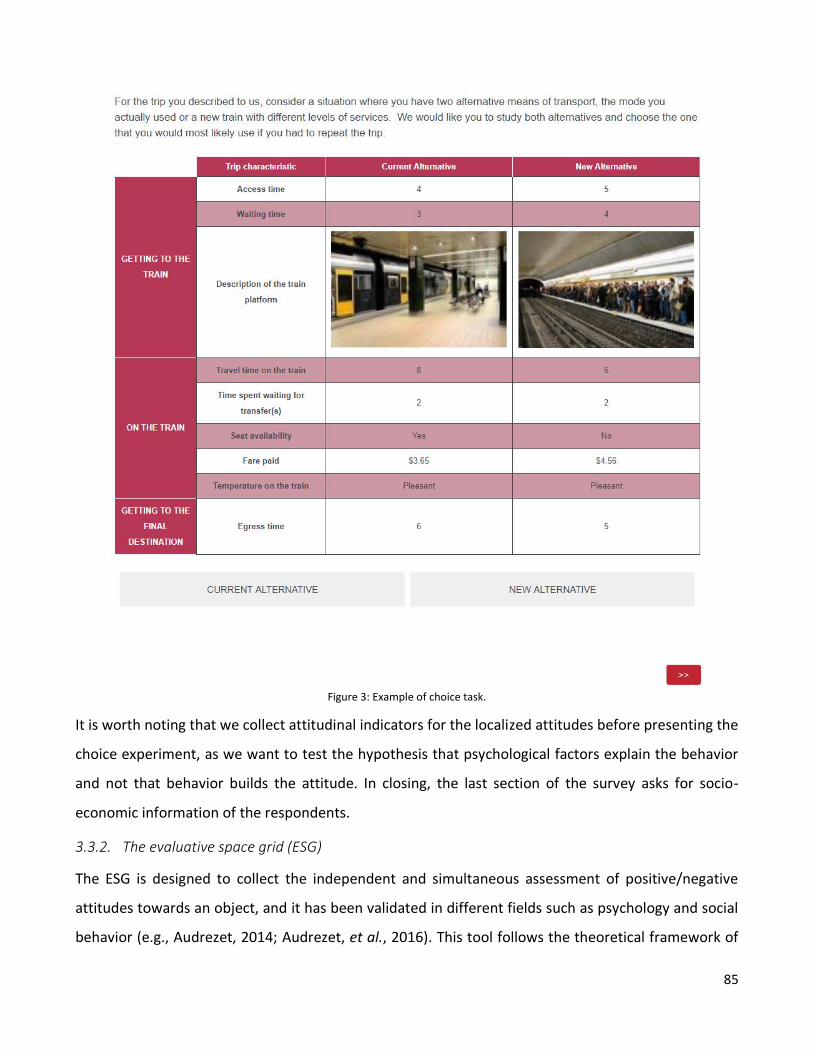
85

Figure 3: Example of choice task.

It is worth noting that we collect attitudinal indicators for the localized attitudes before presenting the

choice experiment, as we want to test the hypothesis that psychological factors explain the behavior

and not that behavior builds the attitude. In closing, the last section of the survey asks for socio-

economic information of the respondents.

3.3.2. The evaluative space grid (ESG)

The ESG is designed to collect the independent and simultaneous assessment of positive/negative

attitudes towards an object, and it has been validated in different fields such as psychology and social

behavior (e.g., Audrezet, 2014; Audrezet, et al., 2016). This tool follows the theoretical framework of

86

Evaluative Space Model (ESM) proposed by Cacioppo and Bernston (1994), who suggested that positive

and negative feelings can be experienced at the same time, also with strong intensities. The ESG

contrasts positive and negative stimuli towards an attitude, posing two 5 points scales on x and y axes.

Subjects are asked to select one of over 25 cells that best reflects their simultaneous negative and

positive feelings towards the stimulus under study, as shown in Figure 4. The grid is designed to

differentiate between four different attitudes: (1) positive (high positive and low negative), (2) negative

(low positive and high negative), (3) indifference (low positive and negative), and (4) ambivalence

(moderate to high positive and negative).

Figure 4: Evaluative space grid. Audrezet (2014) suggests the following division of the grid: bottom left cells identify an indifferent

individual (yellow); bottom right cells classify a subject with a positive attitude (green); the top left cells (red) categorize an individual with a negative attitude; top right cells identify a subject with an ambivalent attitude.

Audrezet et al. (2016) proved that the ESG performs as well as the semantic differential scale with

respect to different criteria (such as reliability and discriminant, convergent, nomological and predictive

validity) and it captures more information (allows to measure separately indifference and ambivalence)

with the advantage of being a single-item measure.

3.3.3. Sample composition

Data was collected using an online panel in April 2017 and consists in a sample of 340 respondents

(mean age 47.3) who recently took a trip by train in Sydney, for any purpose (going from/to work 34.12

percent; working trip 7.06 percent; shopping 7.65 percent; leisure 29.12 percent; visiting friends or

relatives 7.94 percent; other 14.11 percent). Eighty-six percent of respondents has an Australian

citizenship, male respondents account for forty-seven percent of the sample and twenty-three percent

of interviewees state to have never had a bad experience with trains. Fourteen percent of the sample

87

does not provide the income, six percent has no income and the average weekly income of those who

declare it amounts to 1113 AUD. The sample is mainly composed by workers (sixty-three percent) and

retired (seventeen percent), with the remainder being students, full time homemakers and

unemployed and seekers.

3.4. Model

The specification used to analyze the data consists of a structural equation model in which the attitudes

are defined as latent variables and are linked to the attitudinal indicators and to a discrete choice

model. Two latent variables measure the generalized satisfaction/dissatisfaction towards the train

system whilst twelve more latent variables evaluate the localized satisfaction/dissatisfaction for the last

train service the respondents experienced as well as the hypothetical services presented in the SP

experiment. Latent variables describing the satisfaction (either generalized and localized) are linked to

the corresponding attitudinal indicator measuring the positive domain (x axis on the ESG), whilst the

negative domain of the evaluative space grid (y axis) represents the manifestation of the latent variable

measuring the dissatisfaction (either generalized and localized). Figure 5 shows the framework of the

structural equation model: generalized satisfaction and dissatisfaction are defined by individual

characteristics whilst localized satisfaction and dissatisfaction, created in response to a stimulus, also

depend on the attributes of the environment/alternatives. In addition to the parameters measuring the

effect of the latent variable on the corresponding attitudinal indicator, we estimate two different sets

of threshold parameters for the ordered logit models for the positive and negative domains, which we

hypothesize not to vary for different choice tasks.

88

Figure 5: structural equation model framework. The t (= 1, …, 6) for Localized ESG indicates the choice task. Dark and light grey rectangles on the left-hand side represent individual characteristics and attributes of the environment/attitudes, respectively.

The choice model reflects the structure of the stated preference experiment, consisting of two utility

functions representing the train service described by the respondents in section two and a hypothetical

alternative train service. The alternatives depend on individual characteristics, attributes of the train

service as well as of the latent variables measuring the generalized and localized

satisfaction/dissatisfaction. The attributes describing the features of the trip are inserted in both utility

functions and their effect is measured through generic parameters, whereas the individual

characteristics are inserted in the utility function of the reference alternative. It is important to note

that we hypothesize the effect of cost to be heterogeneous among respondents and to be distributed

lognormally.

We assume that the generalized satisfaction and dissatisfaction have an effect on the reference

alternative, whilst the localized attitudes influence the utility of the stated alternatives. The localized

satisfaction and dissatisfaction for the reference alternative are defined using the same set of

parameters of the other localized attitudes (stated alternatives); nonetheless, they do not enter any

utility function. Differently from the localized satisfaction/dissatisfaction for the stated alternatives, we

would expect these attitudes to have a positive effect on the reference alternative. However, such a

specification performs worse than the one adopted in this paper. Therefore, we measure the localized

89

satisfaction/dissatisfaction for the reference alternative with the only scope of capturing the influence

of the regressors and not of explaining the choice process.

In the result section we compare this model (hereafter full model, FM) with five different specifications,

which are briefly illustrated below.

Model 1 (M1) – MNL:

The first model is a multinomial logit model in which the reference and stated alternatives are described

by the attributes listed above as well as socio-economic variables.

Model 2 (M2) – MMNL:

The mixed multinomial logit assumes a random taste variation for the parameter measuring the effect

of cost on the alternatives, specifically defined to follow a lognormal distribution.

Model 3 (M3) – HDCM using only the generalized attitudes:

Model 3 is defined as a hybrid choice model. The structural equations of M3 consist of two latent

variables measuring the generalized satisfaction/dissatisfaction towards the train system explained by

individuals’ characteristics. In the choice model, the latent variables are expected to affect the utility

associated with the reference alternative.

Model 4 (M4) – HDCM using only the localized attitudes towards the last trip taken:

In this model we explore the effect of the localized satisfaction/dissatisfaction towards the last trip on

the utility function of the reference alternative.

Model 5 (M5) - HDCM using the localized attitudes towards the hypothetical train services:

The specification of this model only differs from the FM because of the omission of the generalized

satisfaction/dissatisfaction towards the train system.

3.5. Results

This section includes a specific analysis on the importance of localized attitudes followed by the general

results of the full hybrid choice model. The detailed results of the different models (M1 – M5) are not

presented here for brevity reasons; however, the main findings are discussed.

90

UN

SATISFY

ING

GENERALIZED LOCALIZED (ACT)

5 2.94% 1.47% 1.76% 1.18% 2.94%

UN

SATISFY

ING

5 3.24% 0.59% 0.00% 2.35% 4.41%

4 1.18% 6.18% 5.00% 5.88% 1.47% 4 1.47% 2.35% 3.24% 5.29% 1.47%

3 0.59% 1.47% 15.59% 6.47% 0.88% 3 0.29% 6.47% 12.94% 8.24% 0.88%

2 0.29% 4.12% 2.94% 12.94% 5.29% 2 0.88% 2.65% 2.35% 11.47% 1.76%

1 0.59% 0.88% 1.47% 6.76% 9.71% 1 1.18% 0.29% 3.24% 10.00% 12.94%

1 2 3 4 5 1 2 3 4 5

SATISFYING SATISFYING

UN

SATISFY

ING

LOCALIZED (HYP 1) LOCALIZED (HYP 2)

5 3.24% 0.88% 0.59% 0.88% 1.76%

UN

SATISFY

ING

5 8.82% 1.18% 0.88% 0.88% 2.65%

4 1.47% 5.00% 5.29% 5.88% 1.76% 4 2.06% 7.65% 4.71% 5.29% 0.29%

3 1.18% 5.29% 18.53% 6.47% 0.59% 3 2.65% 6.47% 14.12% 6.18% 0.29%

2 0.88% 4.41% 6.18% 8.53% 0.88% 2 2.35% 4.71% 5.29% 7.06% 1.76%

1 3.53% 0.88% 3.24% 6.76% 5.88% 1 5.00% 0.88% 3.53% 2.65% 2.65%

1 2 3 4 5 1 2 3 4 5


UN

SATISFY

ING


5 12.65% 3.24% 1.18% 0.29% 2.35%

UN

SATISFY

ING

5 7.94% 2.94% 2.06% 1.18% 2.35%

4 5.88% 6.18% 3.53% 6.47% 0.29% 4 4.41% 4.41% 5.29% 3.82% 2.35%

3 2.06% 5.29% 12.65% 2.94% 1.18% 3 1.47% 4.71% 14.12% 5.00% 0.88%

2 1.47% 5.00% 4.41% 5.29% 0.29% 2 1.18% 4.71% 6.76% 6.47% 0.88%

1 7.65% 2.06% 2.94% 2.06% 2.65% 1 5.59% 1.47% 4.12% 2.35% 3.53%

1 2 3 4 5 1 2 3 4 5


UN

SATISFY

ING


5 15.88% 2.94% 0.59% 0.88% 0.88%

UN

SATISFY

ING

5 5.59% 0.88% 0.29% 0.29% 1.18%

4 3.24% 10.00% 2.35% 3.24% 1.18% 4 2.65% 5.00% 3.24% 7.65% 0.29%

3 4.12% 4.71% 14.41% 5.00% 0.29% 3 1.76% 8.24% 14.12% 7.06% 1.18%

2 1.47% 8.53% 3.24% 2.65% 0.88% 2 2.35% 8.53% 5.29% 6.76% 0.29%

1 6.18% 2.65% 2.65% 1.47% 0.59% 1 2.06% 3.24% 3.24% 4.71% 4.12%

1 2 3 4 5 1 2 3 4 5


Table 1: Distribution of responses of the ESGs

91

3.5.1. Localized attitudes

Table 1 shows the distribution of responses of the Evaluative Space Grids used for the analysis. The

color formatting indicates that the greener the cell, the higher the frequency of respondents selecting

that cell. Analyzing the distributions, it clearly emerges the importance of collecting localized attitudes.

Indeed, respondents seem reporting different attitudes according to the specific situation they are

facing, and the differences become more evident when the generalized satisfaction/dissatisfaction is

compared to the localized attitudes for hypothetical train services.

Table 2 compares the generalized attitude and localized satisfaction/dissatisfaction for the last trip

taken. By construction, the numerical difference between the evaluation of two evaluative space grids

ranges from -4 to 4 for both the positive and the negative axes. For example, if a respondent considers

the general train system extremely satisfying and moderately unsatisfying (cell 5:3 in general ESG) and

the first hypothetical alternative very satisfying and very unsatisfying (cell 4:4 in SP1 grid), the difference

will be equal to 1 and -1 for the positive and the negative axes, respectively. The central cell (highlighted

in green) represents the frequency of respondents who reveal the same attitude for the last trip and

for the generalized satisfaction/dissatisfaction towards the trains system. The localized

satisfaction/dissatisfaction for the last trip is slightly different from the generalized

satisfaction/dissatisfaction for forty-eight percent of respondents (difference included within the range

(-1,1) but 0) whilst is very different for nineteen percent of them.

4 0 0 0 1 1 1 0 0 0

3 0 0 0 0 3 1 0 1 0

2 0 0 3 7 9 4 1 0 0

1 0 1 5 16 38 12 1 0 0

0 0 1 1 23 113 28 2 0 0

-1 0 0 2 12 23 11 2 0 0

-2 0 1 0 1 5 0 1 1 0

-3 0 1 0 1 2 0 0 0 0

-4 0 0 0 0 4 0 0 0 0

-4 -3 -2 -1 0 1 2 3 4

Table 2: Matrix of differences between ESGs measuring the generalized satisfaction towards the train and the localized satisfaction towards the last train service experienced. Numbers identify the frequencies of respondents revealing that combination of differences

for x and y axes. A green cell classifies a high frequency, a red cell identifies a low frequency.

Figure 6 reports the matrices of differences among all collected grids, representing either generalized

and localized attitudes. Using a color formatting, it is possible to visually notice the distribution of the

92

frequencies, highlighted by green cells if the frequency is high, and red cells if the frequency is low.

Even though the highest value is always observed at the central cell of any matrix, the presence of non-

null frequencies in most of the remaining cells (light green or yellow) suggests that the localized

attitudes change according to the situation for several respondents.

Figu

re 6

: C

ross

-tab

le in

clu

din

g th

e m

atri

ces

of

dif

fere

nce

s. B

y co

lum

n, t

he

gen

eral

ized

att

itu

de

tow

ard

s th

e tr

ain

ser

vice

(G

ENER

AL)

, th

e lo

caliz

ed a

ttit

ud

e fo

r th

e la

st t

rain

se

rvic

e (R

P)

and

fo

r th

e h

ypo

thet

ical

tra

in s

ervi

ces

(CH

OIC

E TA

SK 1

– 6

). B

y ro

w, t

he

loca

lized

att

itu

de

for

the

last

tra

in s

ervi

ce (

RP

) an

d f

or

the

hyp

oth

etic

al t

rain

ser

vice

s (C

HO

ICE

TASK

1 –

5).

A further evidence emerging from testing the similarity of the generalized and localized attitudes is a

memory effect, or state dependency. The analysis of the average Euclidian distances for any pair of

ESGs collected through the survey (Table 3) reveals that two consecutive grids display a higher similarity

than any other pair (except for choice task 3 - choice task 4, which presents an average Euclidian

distance larger than choice task 3 - choice task 5). As a matter of example, let consider the second

column of Table 3: the average Euclidian distance between the localized attitudes towards the last train

service (RP) and the first hypothetical service (CT1) is 1.287, quite smaller than any other distance in

the column, indicating that the localized attitude towards the last train service is more similar to the

one towards the first hypothetical service than to any other one.

GEN RP CT1 CT2 CT3 CT4 CT5 CT6

GEN

RP 1.038

CT1 1.453 1.287

CT2 1.805 1.741 1.300

CT3 2.049 1.975 1.580 1.322

CT4 1.838 1.775 1.454 1.403 1.370

CT5 2.227 2.286 1.830 1.358 1.261 1.316

CT6 1.794 1.723 1.546 1.453 1.510 1.480 1.414

Table 3: average Euclidian distances

The analysis of the differences of attitudinal indicators highlights the importance of considering

localized attitudes when modelling individual behavior. Indeed, if generalized and localized attitudes

capture different aspects of the mental process leading to the choice, the omission of such factors may

potentially lead to incorrect estimates, as their contribution in explaining the choice will be absorbed

by the error term.

3.5.2. Structural equation model

Table 4 reports the coefficient estimates for the structural model. The generalized satisfaction is

negatively affected by the number of cars in respondent’s household as well as by the past experience

travelling by train. A higher probability of having a lower generalized satisfaction towards trains is

revealed by respondents who have more cars available in the household and by those who have had a

95

bad experience travelling by train, with more recent experiences (less than six months) impacting more

than older ones (more than six months ago). Conversely, a bad experience within the last six months

increases the probability that an individual has higher generalized dissatisfaction towards trains. This

latent variable is also affected by a logarithmic transformation of age (the older the respondent, the

lower the generalized dissatisfaction) and by the individual occupation (students have a higher

probability of revealing a lower generalized dissatisfaction). The latent variables measuring the

localized satisfaction and dissatisfaction are negatively affected by age and a logarithmic

transformation of age, respectively. That is, an older respondent has a higher probability of displaying

an indifferent attitude towards the train system, whilst an ambivalent attitude is more likely to be held

by a younger individual. As for the generalized dissatisfaction, those who have had a bad experience

with a train service in the last six months are more likely to display a higher localized dissatisfaction

towards the train service. The weather affects the localized satisfaction/dissatisfaction: indeed,

travelling in an overcast day has a negative impact on the localized satisfaction whilst a rainy day has a

positive effect on the localized dissatisfaction. As concerns other features of the trip, the localized

satisfaction is influenced by the crowd on the platform (the lower the better) and negatively by the

waiting time. A pleasant temperature on the train (reference alternative) increases the localized

satisfaction whilst only a high temperature seems to have a negative impact on the localized

dissatisfaction. Finally, the parameters capturing the correlation between the positive and negative

domains of the latent variables (i.e. within generalized satisfaction/dissatisfaction and localized

satisfaction/dissatisfaction) are not statistically different from zero, suggesting that the mental

processes bringing to the positive and negative assessments on the ESGs are independent.

96

Structural model

Generalized

Satisfaction

Generalized

Dissatisfaction Localized Satisfaction

Localized

Dissatisfaction


Age - - - - -0.016 (-6.42) - -

Log(Age) - - -0.607 (-1.87) - - -0.382 (-2.22)

Cars in the hh -0.197 (-1.96) - - - - - -

Occupation = student - - -0.838 (-1.63) - - - -

Bad exp. Train 6 months -0.728 (-2.21) 0.817 (2.70) - - 0.241 (2.09)

Bad exp. Train > 6 m -0.452 (-1.65) - - - - - -

Weather = Overcast - - - - -0.249 (-2.24) - -

Weather = Rainy - - - - - - 0.199 (1.66)

Crowd = Low - - - - 0.555 (7.06) - -

Crowd = Medium - - - - 0.256 (4.02) - -

Temperature = Low - - - - -0.870 (-8.45) - -

Temperature = High - - - - -0.872 (-10.07) 0.427 (6.11)

Waiting time - - - - -0.026 (-3.47) - -

Correlation parameters

ρ0 -0.195 (-1.14)

ρ1 -0.038 (-0.51)

Table 4: coefficient estimates for the latent variables.

Based on the findings reported in the previous section where respondents revealed a memory effect

compiling the localized attitudinal indicators, we inserted a further variable assessing the similarity

between consecutive perceptual indicators in any latent variable measuring the localized

satisfaction/dissatisfaction. Specifically, the absolute value of the difference between two consecutive

ESGs (for both the positive and the negative indicators) is found to be significant for eleven out of twelve

localized latent variables (Table 5). Otherwise stated, the similarity of two consecutive assessments

influences the localized satisfaction/dissatisfaction through the stated preference experiment. Keeping

the ESG shown in Figure 4 in mind, the sign of the parameters suggests the position of the individuals

who are more likely to give different assessment for two consecutive levels of (hypothetical) train

services. As a matter of example, the parameter Difference Satisfaction 2_1 suggests that larger is the

1, 2,( )sat satabs y y , higher is the probability that the individual has a lower localized satisfaction for the

train service presented in choice task 2. Similarly, larger is the 1, 2,( )dis disabs y y , higher is the probability

that the subject considers the same train service dissatisfying. Considering these results, it is possible

97

to conclude that the respondents who assess ESG1 and ESG2 differently, are more likely to describe the

train service presented in choice task 2 dissatisfying. Opposite is the case of the assessment of ESG6

where the parameters measuring the effects of 5, 6,( )sat satabs y y on the localized

satisfaction/dissatisfaction of the hypothetical train service shown in choice task 6 are positive and

negative, respectively. As a result, respondents who assess ESG5 and ESG6 differently, are more likely

to describe satisfying the train service presented in choice task 6.

, 1,

, 1,

( )

( )

t sat t sat

t dis t dis

abs y y

abs y y

Par. (Rob. t-test)

Difference Satisfaction 1_RP -0.668 (-4.53)

Difference Dissatisfaction 1_RP 0.171 (1.99)

Difference Satisfaction 2_1 -0.346 (-3.26)

Difference Dissatisfaction 2_1 0.432 (5.94)



Difference Satisfaction 4_3 0.180 (2.83)

Difference Dissatisfaction 4_3 -0.027 (-0.24)



Difference Satisfaction 6_5 0.494 (8.60)

Difference Dissatisfaction 6_5 -0.51 (-2.33)

Table 5: coefficient estimates for the differences of two consecutive indicators.

Table 6 contains the coefficient estimates for the measurement model. The parameters measuring the

effect of the latent variables on the attitudinal indicators are significant and positive, indicating that a

greater generalized/localized satisfaction/dissatisfaction increases the probability that respondents

attribute a higher value to the corresponding attitudinal indicator. The estimates of the two sets of

thresholds for the ordered logit models are shown in the bottom part of Table 6.

98

Measurement model

Par. (Rob. t-test)

Generalized Satisfaction 1 1.17 (7.24)

Generalized Dissatisfaction 1 0.936 (6.54)

Localized Satisfaction RP 1.38 (10.90)

Localized Dissatisfaction RP 1.78 (11.09)

Localized Satisfaction t=1 1.21 (9.36)

Localized Dissatisfaction t=1 1.76 (12.38)












Satisfaction Dissatisfaction

Par. (Rob. t-test) Par. (Rob. t-test)

τ1 -5.49 (-16.29) -4.04 (-3.45)

τ2 -3.61 (-9.65) -2.49 (-2.11)

τ3 -1.61 (-11.65) -0.75 (-6.43)

τ4 0.68 (4.29) 0.90 (7.39)

Table 6: coefficient estimates for the measurement model.

3.5.3. Choice model

The estimates of the full hybrid choice model are displayed in the last column of Table 7. The

parameters measuring the effect of egress and travel times on the alternatives are significant and

negative, indicating a decreasing utility for an increase in these attributes. Similarly, an increase in cost

is perceived as a detriment, even if individuals display heterogeneous sensibility to this parameter.

Indeed, the parameter related to cost is assumed lognormal distributed, resulting in a distribution with

a positive skew. Having a seat available on the train increases the probability of having a higher utility.

As concerns the socioeconomic characteristics, respondents who always select the same alternative in

the six choice tasks (non-traders) and those who prefer to be by themselves rather than being in

crowded places (comfortable = alone) have a higher probability of choosing the reference alternative

whilst those who prefer individual but not motorized transportation means (i.e. taxi or Uber service)

for visiting friends and relatives display a lower probability of choosing this alternative. Other

99

socioeconomic characteristics do not seem to have a direct impact on the process of choice, but they

do have an indirect impact via generalized and localized attitudes. The estimates of the generalized

satisfaction and dissatisfaction indicate that higher the satisfaction (dissatisfaction), higher (lower) the

probability of choosing the reference alternative. An important finding of this work is the significant

effect of the localized attitudes on the individual preferences. A higher satisfaction (dissatisfaction)

measured for the hypothetical train services increases (decreases) the probability of choosing the

stated alternative. To the best of our knowledge, no previous paper has measured the impact of

localized attitudes on the decision-making process in the context of transportation.

Choice model

Attributes M1 M2 M3 M4 M5 FM

ASC RP -0.304 (-1.42) -1.65 (-2.15) 0.195 (0.60) 4.27 (2.73) -0.103 (-0.49) 0.405 (0.41)

Access Time -0.031 (-1.73) - - - - -

Travel Time -0.036 (-5.40) -0.0386 (-5.23) -0.040 (-5.09) -0.040 (-5.02) -0.033 (-4.75) -0.023 (-3.02)

Egress Time -0.028 (-3.63) -0.029 (-3.05) -0.039 (-3.80) -0.038 (-3.92) -0.036 (-4.14) -0.030 (-3.52)

Cost (μ) -0.246 (-3.90) -1.687 (-4.17) -1.43 (-4.23) -1.44 (0.344) -1.447 (-4.73) -1.655 (-4.52)

Cost (σ) - 1.820 (4.87) 1.64 (5.17) 1.66 (5.02) 1.422 (4.96) 1.642 (4.67)

Seat availability 0.612 (5.43) 0.701 (5.29) 0.632 (4.83) 0.603 (4.60) 0.753 (6.04) 0.683 (5.50)

Temperature Low -0.535 (-4.77) -0.674 (-5.47) -0.836 (-3.97) - - -

Temperature High -1.02 (-6.06) -1.16 (-5.83) -1.650 (-4.28) - - -

Crowd Low 0.247 (2.58) 0.433 (3.21) - - - -

Crowd Medium - 0.278 (2.17) - - - -

Individual characteristics

Non-Trader 1.86 (5.12) 1.86 (4.91) 2.610 (8.57) 2.60 (8.87) 2.015 (5.11) 1.927 (5.18)

Train for leisure trips - - - - 0.404 (1.65) -

Car for leisure trips - - 0.307 (1.64) 0.314 (1.81) 0.425 (1.95) -

Train for working trips - - - - -0.310 (-2.07) -

Age 0.008 (1.73) - - - - -

Log(Age) - 0.341 (1.70) - - - -

Uber/Taxi for visiting -1.90 (-7.73) -1.42 (-4.99) -1.840 (-5.04) - - -1.13 (-4.42)

Occ. = Student 0.452 (1.84) 0.519 (1.95) 0.501 (1.65) - - -

Comfortable = Alone - - - - - -0.235 (-1.65)

Latent variables

Generalized pos. attitude - - 1.92 (2.04) 2.17 (3.45) - 0.451 (1.92)

Generalized neg. attitude - - 1.70 (1.71) 1.89 (2.99) - -0.428 (-1.81)

Localized pos. attitude - - - - 0.026 (0.31) 0.315 (2.35)

Localized neg. attitude - - - - -0.045 (-0.52) -0.463 (-2.39)

Willingness to pay

8.79 AUD/h 12.54 AUD/h 10.01 AUD/h 10.15 AUD/h 8.52 AUD/h 7.22 AUD/h

Table 7: coefficient estimates for the choice model. In brackets robust t-test.

100

3.5.4. Discussing the different models

In this paragraph, we present the results of the best specification derived for any model and discuss the

major differences. However, performances of these models are not directly comparable. In models M4

– M5 (as for the FM), the temperature on the train and crowd on the platform affect the choice through

the localized satisfaction/dissatisfaction. In models M1 – M2 – M3 instead, in addition to travel and

egress times, cost and seat availability, the attributes access time (only in M1), crowd on the platform

(in M1 – M2) and temperature on the train directly influence the utility functions of the alternatives.

According to the results of both models, respondents prefer less crowd on the platform and pleasant

temperature on the train.

Looking at M3 and M4, the parameters measuring the effect of the generalized satisfaction (for M3)

and the localized satisfaction for the last trip (for M4) indicate that higher the satisfaction, higher the

probability of choosing the reference alternative. A similar pattern emerges also for the parameters

related to the generalized and localized (for the last trip) dissatisfaction, even if the magnitude is lower.

Specifically, M3 suggests that a respondent, with a pronounced generalized dissatisfaction towards

trains, prefers the reference alternative to the SP. This result may indicate that the last trip that the

respondent took by train was, conversely, a satisfying experience. However, the partial information on

the attitudes captured in M3, which does not consider localized attitudes for the last trip, makes the

result less straightforward to explain. Along the same line, a respondent with higher dissatisfaction for

the last trip who still prefers the reference alternative (M4) can be interpreted as a nonsense. Again,

M4 does not include the localized attitudes for the stated alternatives, which can be perceived even

worse than the last trip experienced by the respondent.

Finally, the latent variables proxying the localized satisfaction/dissatisfaction have no significant effect

on the choice of the alternative (M5). This latter result embodies a further proof of the importance of

considering generalized and localized attitudes altogether when exploring individual preferences.

Indeed, when the effects of the generalized/localized attitudes are analyzed separately, the parameters

may not be able to capture sufficient information or their effects can be the sum of different aspects

and therefore, the impact of the psychological factors on the mode choice can become biased.

An interesting discussion concerns the value of the willingness to pay (WTP) estimated using different

models and reported in the last row of Table 7. The values refer to the median of a lognormal

distribution for the models including a random parameter for cost (from M2 to FM) and to the mean

101

value for the multinomial logit model. Focusing on the models including a random parameter for cost,

it is worth noting that increasing the number of latent variables used in the structural equation model,

the WTP decreases. That is, whilst the mixed multinomial logit suggests that the median respondent is

willing to pay 12.54 AUD for saving one-hour of travel time, the hybrid choice models including two

latent variables, measuring respectively the generalized and the localized (towards the last trip taken)

satisfaction/dissatisfaction (M3 – M4), suggest a WTP of about 10 AUD. According to M5, which includes

twelve latent variables determining the localized satisfaction/dissatisfaction for the hypothetical

alternatives, the median respondent is willing to pay 8.52 AUD to save one hour of trip by train, which

is about 15% less than the value found for specifications M3 and M4. An even lower WTP emerges from

the FM, in which both the generalized and the localized satisfaction and dissatisfaction are included.

Here, fourteen latent variables are specified, resulting in a WTP of 7.22 AUD, which is about 25% less

than the model including only the generalized attitudes. This result is consistent with the literature

(Abou-Zeid et al., 2010; Walker et al., 2010; Guevara, 2015; Vij, Walker, 2016) showing that the inclusion

of latent variables and measurement indicators reduces the bias due to omitted variables or

measurement error. In our case, additional significant latent variables further reduce the measurement

bias. The information added by considering localized attitudes is likely to be dispersed in the error term

of the alternative in a model that do not consider psychological factors at all or does only consider

generalized attitudes, generating a less precise value for the willingness to pay for saving travel time.

Such a finding may also question the accuracy of the WTP estimated in similar settings within

transportation literature given that the common practice is to include only generalized attitudes when

estimating HDCMs.

3.6. Conclusions

This chapter focuses on the role of attitudes in determining individual choice behavior and examines

the temporal stability of generalized attitudes within a stated choice experiment framework. Within

the psychological literature, there exist three different schools of thought as to whether or not attitudes

are largely fixed or somewhat transient. The first school of thought identified assumes that attitudes

are long term stable constructs which are “memory-based” such that an attitude towards an object is

linked to one or more global evaluations that brought to the mind once the object is encountered. The

second school of thought related to the temporal stability of attitudes assumes that attitudes are short

102

term situational specific concepts that are constructed at the time a specific situation occurs and that

evaluative judgments are formed only when required rather than being stored in longer term memory.

The third school of thought on attitude formation suggests that attitudes are created via a mixture of

both short and long-term influences, assuming that evaluative processes towards objects are part of an

iterative cycle where the current evaluation of stimuli can be adjusted as new contextual and

motivational information arises.

The current chapter reports the results of a stated choice experiment where respondents are asked to

provide their generalized and localized attitude towards a train service. The approach adopted allows

for an examination as to how attitudinal responses vary as the attribute levels of the alternatives

presented within the experiment change over repeated choice tasks. Comparing the attitudinal

indicators, it emerges that the generalized and localized attitudes are different for most of the

respondents and the farer the hypothetical train services are presented in the stated preference

experiment, the weaker the stability of the attitude is. In addition, this divergence also appears

comparing localized attitudes specific of the hypothetical situations and it increases when comparing

two hypothetical train services more distant in time. The comparison of attitudinal indicators highlights

the necessity of exploring the effect that localized attitudes have on individual choice. The results of

the stated preference experiment conducted in this work reveal that both generalized and localized

attitudes have a significant impact on individuals’ choices. In our experiment, the models analyzing

generalized and localized attitudes separately only capture partial information related to the

psychological process leading to the choice and, consequently, the interpretation of the results may be

tricky. Furthermore, the omission of localized attitudes may potentially lead to inconsistent estimates,

as their contribution in explaining the choice will be absorbed by the error term. A demonstration is

given by the value of the WTP obtained by different hybrid choice model specifications, which

decreases as the number of latent variables measuring attitudes increases. Specifically, a model

including generalized and localized attitudes presents a willingness to pay about 25% lower than a

specification including only generalized attitudes and 40% lower than a specification without any

attitude.

The evidence of this work proves the importance of specifying both generalized and localized attitudes

when exploring the role of psychological factors on the decision-making process. The inclusion of

attitudes with different temporal stability provides more consistent estimates and it appears to be

103

critical to transportation planning and research given the link between attitudes and behavior as

explained by the theory of planned behavior. Indeed, if attitudes are a precursor towards action, one

mechanism to change travel behavior may be via the ability of transport planners to change attitudes,

using for example the introduction of new stimuli, such as a message or advertisement, which when

processed by the individual, can result in an attitude change alongside a change in behavior.

104

References

Abou-Zeid, M., Ben-Akiva, M., Bierlaire, M., Choudhury, C., Hess, S., 2010. Attitudes and value of time heterogeneity. Applied

Transport Economics A Management and policy perspective, 523 – 545.

Ajzen I., 1985. From Intentions to Actions: A Theory of Planned Behavior. In: Kuhl J., Beckmann J. (Eds.) Action Control. SSSP

Springer Series in Social Psychology. Springer, Berlin, Heidelberg.

Allport, G.W., 1935. Attitudes. In Handbook of Social Psychology, C Murchinson, 798 – 844. Worcester, MA: Clark Univ. Press.





Bahamonde-Birke, F.J., Kunert, U., Link, H., Ortúzar, J., 2017. About attitudes and perceptions – Finding the proper way to

consider latent variables in discrete choice models. Transportation 44, 475–493. DOI 10.1007/s11116-015-9663-5

Ben-Akiva, M., Boccara, B., 1993. Discrete choice models with latent choice sets. Working paper, Department of Civil

Engineering, Massachusetts Institute of Technology, Cambridge, MA.

Ben-Akiva, M., Morikawa, T., 1990. Estimation of travel demand models from multiple data sources. International

Symposium on Transportation and Traffic Theory, Yokohama, Japan.

Ben-Akiva, M.E., Walker, J.L., Bernardino, A.T., Gopinath, D.A., Morikawa, T. and Polydoropoulou, A., 2002. Integration of

choice and latent variable models. In H.S. Mahmassani (ed.), In Perpetual Motion: Travel Behaviour Research

Opportunities and Challenges. Pergamon, Amsterdam.

Bohner, G., Dickel, N., 2011. Attitudes and attitude change. Annual Review of Psychology 62, 391 – 417.



2909.115.3.401

Chen, S., Chaiken, S., 1999. The heuristic-systematic model in its broader context. In S. Chaiken & Y. Trope (Eds.), Dual

process theories in social psychology, 73 - 96. New York: Guildford Press.

Conrey, F.R., Smith, E.R., 2007. Attitude representation: attitudes as patterns in a distributed, connectionist representational

system. Social Cognition 25, Special Issue: What is an Attitude?, 718-735.

https://doi.org/10.1521/soco.2007.25.5.718.

Crano, W.D., Prislin, R., 2006. Attitudes and Persuasion. Annual Review of Psychology 57, 345 – 374.

Cunningham, W.A., Zelazo, P.D., 2007. Attitudes and evaluations: a social cognitive neuroscience perspective. Trends in

Cognitive Sciences 11, 97 – 104.

Cunningham, W.A., Zelazo, P.D., Packer, D.J., Van Bavel, J.J., 2007. The iterative reprocessing model: a multilevel framework

for attitudes and evaluation. Social Cognition 25(5), 736 – 760.

Currim, I., 1981. Using segmentation approaches for better prediction and understanding from consumer mode choice

models. Journal of Marketing Research 18, 301-309.

https://doi.org/10.1521/soco.2007.25.5.718

105

Daly, A., Hess, S., Patruni, B., Potoglou, D., Rohr, C., 2012. Using ordered attitudinal indicators in a latent variable choice

model: a study of the impact of security on rail travel behaviour. Transportation 39(2), 267-297.

Daziano, R. A., Bolduc, D., 2013a. Incorporating pro-environmental preferences toward green automobile technologies

through a Bayesian Hybrid Choice Model. Transportmetrica A: Transport Science 9(1), 74 - 106.

Daziano, R. A., Bolduc, D., 2013b. Covariance, identification, and finite-sample performance of the MSL and Bayes estimators

of a logit model with latent attributes. Transportation 40(3), 647-670.

Fazio, R.H., 1990. Multiple processes by which attitudes guide behavior: The MODE model as an integrative framework. In

M.P. Zanna (Ed.), Advances in experimental social psychology. 23, 75-109. New York: Academic Press.

Gawronski, B., Bodenhausen, G.V., 2007. Unraveling the processes underlying evaluation: attitudes from the perspective of

the APE model. Social Cognition 25, 687–717.

Green, P., 1984. Hybrid Models for Conjoint Analysis: An Expository Review. Journal of Marketing Research 21, 155-169.

Green, P., Goldberg, S., Montemayor, M., 1981. A Hybrid Utility Estimation Model for Conjoint Analysis. Journal of Marketing

45(1), 33-41. doi:10.2307/1251718

Guevara, C.A., 2015. Critical assessment of five methods to correct for endogeneity in discrete choice models.

Transportation Research Part A 82, 240 – 254.

Hensher, D., 1990. Hierarchical stated response design – an application to bus user preferences. Logistics and Transportation

Review 26(4), 299 – 321.



Maldonado-Hinarejos, R., Sivakumar, A., Polak, J.W., 2014. Exploring the role of individual attitudes and perceptions in

predicting the demand for cycling: a hybrid choice modelling approach. Transportation 41, 1287–1304. DOI

10.1007/s11116-014-9551-4

McFadden, M., 1980. Econometric models for probabilistic choice among products. The Journal of Business 53(3-2):

Interfaces between marketing and economics, S13 - S29.

McFadden, M., 1986. The choice theory approach to market research. Marketing Science 5(4). Special issue on consumer

choice models, 275 – 297.

Morikawa, T., 1989. Incorporating stated preference data in travel demand analysis. Unpublished phD dissertation, Dept. of

Civil Engineering, Massachusetts Institute of Technology, Cambridge, MA.

Morikawa, T., Ben-Akiva, M., Mc Fadden, D., 1990. Incorporating psychometric data in econometric demand models.

Prepared for presentation at the Banff Invitational symposium on consumer decision-making and choice behavior,

Canada.

Ngene 1.1.2 User Manual & Reference Guide, 2014. http://www.choice-metrics.com/download.html

Petty, R.E., Briñol, P., DeMarree, K.G., 2007. The meta-cognitive model (MC) of attitudes: implications for attitude

measurement, change, and strength. Social Cognition 25.

Petty, R.E., Wegener, D.T., 1999. The elaboration likelihood model: current status and controversies. In S. Chaiken & Y. Trope

(Eds.), Dual process theories in social psychology, 41 -72. New York: Guildford Press.

http://www.choice-metrics.com/download.html

106

Raveau, S., Yanez, M., Ortúzar, J., 2012. Practical and empirical identifiability of hybrid discrete choice models.

Transportation Research Part B: Methodological 46, 1374–1383. DOI: 10.1016/j.trb.2012.06.006.

Red3, 2005. Evaluation of Australian TravelSmart Projects in the ACT, South Australia, Queensland, Victoria and Western

Australia: 2001–2005, Report to the Department of Environment and Heritage and State TravelSmart Program

Managers. Accessed from: http://www.travelsmart.gov.au/publications/evaluation-2005.html

Rose, J.M., Bliemer, M.C.J., 2008. Stated preference experimental design strategies, in Hensher, D.A. and Button, K.J. (eds.)

Handbook of Transport Modelling, Elsevier, Oxford, Ch. 8, 151-180.

Rose, J.M., Bliemer, M.C.J., Hensher, D.A., Collins, A.C., 2008. Designing efficient stated choice experiments involving

respondent based reference alternatives. Transportation Research Part B 42(4), 395-406.

Schacter, D.L., Gilbert, D.T., Wegner, D.M., 2011. Psychology (2nd edition). New York: Worth.

Schwarz, N., 2007. Attitude construction: evaluation in context. Social Cognition 25(5), 638 – 656.

Swait, J., 1994. A structural equation model of latent segmentation and product choice for cross-sectional revealed

preference choice data. Journal of retailing and consumer services 1(2), 77 – 89.

Train, K.E., McFadden, D.L., Goett, A.A., 1987. Consumer attitudes and voluntary rate schedules for public utilities. The

review of economics and statistics 69(3), 383 – 391.

Van Acker, V., Mokhtarian, P.L., Witlox, F., 2011. Going soft: on how Subjective Variables Explain Modal Choices for Leisure

Travel. European journal of transport and infrastructure research 11(2), 115-146.

Vieira, L., 1992. The value of service in freight transportation. PhD dissertation, Dept. of Civil Engineering, Massachusetts

Institute of Technology, Cambridge, MA.

Vij, A., Walker, J.L., 2016. How, when and why integrated choice and latent variable models are latently useful.

Transportation Research Part B 90, 192 – 217.

Walker, J.L., 2001. Extended Discrete Choice Models: Integrated Framework, Flexible Error Structures, and Latent Variables.

Massachusetts Institute of Technology.

Walker, J., Li, J., Srinivasan, S., Bolduc, D., 2010. Travel demand models in the developing world: correcting for measurement

errors. The International Journal of Transportation Research 2(4), 231 – 243.

https://biblio.ugent.be/publication?q=parent+exact+%22EUROPEAN+JOURNAL+OF+TRANSPORT+AND+INFRASTRUCTURE+RESEARCH%22

107

Conclusion

This dissertation focuses on the way psychological factors, in particular attitudes, are treated in choice

modeling in the context of transportation. Here, the common practice adopted is still very distant from

the one used in psychological literature and therefore it is not always accurate. The dissertation

proposes procedures and methods to improve the measurement of psychological variables to be used

in choice modeling. The use of the Evaluative Space Grid to collect attitudinal indicators represents the

main contribution of this dissertation, as this has been employed in all the works. The first two chapters

show in details the benefits of using this tool when modeling individual preferences. If the researcher

aims at suggesting policies for different segments of the population based on psychological variables

(for example environmental friendly, attached to the car, pro adventures, etc.), then the ESG is the

perfect tool to employ. Indeed, this instrument improves the segmentation helping policy makers to

draw more specific and effective policies. The last chapter is no longer focused on the instrument itself,

rather it shows the importance of considering different types of attitudes when modeling individual

preferences. Nevertheless, the ESG can be modeled as suggested in chapters one and two to take into

account the possibility that respondents can have a neutral satisfaction as the outcome of two different

attitudes, which are indifference and ambivalence.

The importance that psychological variables have on individual behavior is the foundation of this

dissertation. Since McFadden proposed the framework of hybrid discrete choice models (1986), several

papers showed the role that attitudes, perceptions and beliefs have on determining individual

preferences and choices in a transportation context. One of the most used techniques that connects

the exploration of psychological factors to the study of individual preferences is hybrid discrete choice

modeling. Whilst the choice modeling part has been improved in the last decades, introducing for

examples mixed models, latent class models and discrete-continuous models, not much attention has

been paid for the structural equation model, which aims at exploring the psychological aspects of the

respondent. The trigger of this research is the opportunity to improve the analysis of psychological

factors which drive individual choices.

This dissertation contributes to this literature in a threefold way. The first contribution is instrumental,

by suggesting the use of the Evaluative Space Grid for measuring attitudes, the second one is

methodological, by showing the econometric steps for including such an instrument in the framework

108

of a hybrid choice model, and the final one is structural, by recommending the use of long-term stable

and short-term situational specific attitudes when exploring the role of psychological factors on

individual behavior.

The first chapter focuses on the importance of distinguishing between individuals having indifferent

and ambivalent attitudes, as well as positive and negative inclinations. Traditional methods for

measuring attitudes, such as Likert scale, semantic differential scale or conversely framed questions,

help the researcher to segment the population of individuals having positive and negative attitudes,

however these tools aggregate individuals revealing a neutral inclination. The Evaluative Space Grid

(ESG), proposed by Larsen et al. (2009), instead, allows the researcher to detect various attitudinal

outcomes towards an object, including ambivalence and indifference, alongside the more commonly

measured positive and negative attitudinal outcomes. Such an instrument has already been used in

psychology and in marketing studies to assess ambivalence and indifference by means of a deterministic

score. However, assuming attitudes are latent constructs, hence not directly measurable, the use of

scores seems anachronistic. The first chapter includes an approach, based on two simultaneous ordered

logit models, which considers the latent nature of the attitudes. Using this procedure, it is possible to

model up to a probability any attitudinal outcome. An additional advantage of the proposed model, is

its ability to forecast future responses (i.e. predict out of sample). In many applied fields, such as

environmental or transport economics in which such psychological methods are commonly used, being

able to predict how attitudes may develop or change over time, or even what attitudes may exist in

other non-sampled populations, can support policy makers in their decisions.

The second chapter of this dissertation describes the methodology to include the ESG in the framework

of hybrid choice models. In brief, structural equations consist of two latent variables, representing

positive and negative domains respectively, explained by individual characteristics and linked by a

correlation term; measurement equations consist of two ordered logit regressions which connect the

observables items to the latent variables. In addition to the methodological contribution, this chapter

tests the hypothesis that individuals having indifferent and ambivalent attitudes display different

preferences in a context of transportation mode choice for commuting trips. Furthermore, these

categories also respond differently if the proposed alternatives experience a change in the attributes

of the alternatives. The inclusion of attitudes in studies modeling individuals’ preferences is very helpful

for policy purposes. Indeed, policy makers may target their campaign specifically for individuals who

109

have, for instance, a strong positive or negative inclination towards environmental concerns or

attachment to the car. This work helps policy makers draw even more powerful and effective policies,

showing that it is important to consider also the segment of individuals having a neutral inclination, i.e.

subjects revealing an ambivalent or indifferent attitude, as their choices and their reaction to an

incentive may be different.

The last chapter of the dissertation enters a debate in psychological literature on the temporal stability

of attitudes. Here, a hybrid choice model explores the impact that long-term stable constructs

(generalized attitudes) and short-term situational specific concepts (localized attitudes) have on

individual behavior. Generalized and localized attitudes are measured through a stated preference

experiment in the context of transportation. Whilst the inclusion of stable psychological constructs is

common practice, the exploration of the role of attitudes constructed on the spot is new to

transportation literature. Evidence shows that generalized and localized attitudes are different for most

respondents and that both types of attitudes have a significant impact on individuals’ choices.

Furthermore, the omission of localized attitudes may potentially lead to inconsistent estimates, as their

contribution in explaining the choice will be absorbed by the error term, as demonstrated by the value

of the WTP obtained by different hybrid choice model specifications. Specifically, evidence shows that

including both types of attitudes decreases the amount that respondents are willing to pay to save

travel time. The inclusion of attitudes with different temporal stability appears to be critical to

transportation planning and research given the link between attitudes and behavior as explained by

the Theory of Planned Behavior. Indeed, if attitudes are a precursor towards action, one mechanism to

change travel behavior may be via the ability of transport planners to change attitudes, using for

example the introduction of new stimuli, such as a message or advertisement, which when processed

by the individual, can result in an attitude change alongside a change in behavior.

The methodology and the procedures presented in this dissertation, together with the empirical case

studies proposed, represent a tiny contribution to what is possible to achieve importing ad hoc

procedures from psychology to applied fields like transportation. Psychological literature contains

numerous debates on factors influencing individual behavior, such as attitudes, perceptions, beliefs and

social norms, and therefore further effort and investigation is required by applied researchers in this

direction. Several advances have been done in modeling individual behavior in the last decades, and

110

importing new instruments or testing theoretical frameworks suggested by psychologists may further

contribute to improve the representation of individual behavior.

Documents

The role of attitudes in determining individual behavior ... · Prof. Rico Maggi, supervisor ... Structure of the questionnaire: ... Data were collected through a survey conducted