Embed Size (px)
Citation preview

1
The Role of Human Capital and Physical Capital Accumulation in
an R&D-based Growth Model
Thanh Le* School of Economics
Australian National University
Abstract
This paper presents a Schumpeterian endogenous growth model where technological progress
creates higher quality versions of intermediate inputs. Human capital, the key production
factor that is used for different activities, is allowed to evolve over time using knowledge and
physical investment as two additional inputs. Long-run growth is determined by education
and research technologies, consumers’ preferences, as well as flat-rate income tax and R&D
subsidy. The paper argues that economies need both to accumulate human capital and do
research in order to obtain long-run balanced growth and there always exists a growth
maximizing income tax/R&D subsidy rate.
Keywords: Economic growth, human capital accumulation, physical capital accumulation,
R&D.
JEL classification: O11, O15, O31, O38, O41.
* Contact: Thanh Le, School of Economics, LF Crisp Building 2115, Australian National University, ACT 0200, Australia. Phone: 61-2-612 55121. Email: [email protected]. This paper is part of my PhD dissertation at School of Economics, Australian National University. The author is grateful for valuable comments of Steve Dowrick, Flavio Menezes, Akihito Asano, and all seminar participants in Economics PhD Seminar series. This research is funded by an ANU Research Scholarship. The author is responsible for any remaining errors.

2
1- Introduction
Over the past two decades, economic history has experienced a blossom of new growth
theory. This growing literature can be divided into two distinct streams. Models of the first
stream place emphasis on the endogenous accumulation of production factors (physical
capital and human capital) such as in Lucas (1988), Barro and Xala-i-Martin (1995, ch.5),
Bond, Wang, and Yip (1996). Examples of models of the second type are Romer (1990),
Grossman and Helpman (1991), and Aghion and Howitt (1992, 1998a, b), etc. They share a
common feature that technological progress resulting from purposive research activities is the
major engine of growth. In these models, innovations take either forms of quality
improvements to existing products (quality ladder) or introduction of new goods (expanding
varieties).
An important gap in this literature lies in the division: while the first stream pays attention to
the roles of production factors in growth process and neglects the effect of R&D, the second
investigates R&D assuming factor inputs are in fixed supply. Bridging the gap by considering
those issues in an integrated framework is the purpose of this paper. This paper sets up a
comprehensive model of endogenous technological progress with human capital and physical
capital accumulation. Human capital and technology (knowledge) are two complementary and
interacting factors. While human capital is the main factor for knowledge production,
knowledge enhances human capital through education and training. This analysis is important
for understanding the combined effects of those forces in promoting growth as well as the
allocation of production factors across economic activities.
The model presented here is one among the quality ladder models in which technological
progress only creates higher quality versions of intermediate inputs. The structure follows
Howitt and Aghion (1998) and Howitt (1999) but it departs from their framework by allowing
the stock of human capital to be endogenously determined. Therefore, growth persists in this

3
model for three reasons: increases in quality, physical capital accumulation and human capital
accumulation. The main contribution of the paper is an analysis of the role of human and
physical capital accumulation in explaining growth in an R&D-based growth context.
To be more specific, the economy under consideration has a constant population. It consists of
an education sector and three other productive sectors: a final goods sector, an intermediate
goods sector, and finally, a research sector. While the final goods sector and the R&D sector
are competitive, the intermediate goods sector is monopolistic. Final goods are homogenous
and produced using intermediate goods and a production factor of fixed supply (such as land
or water surface). The output from the final goods sector is used for consumption and
investment, which takes place under two forms: accumulating physical capital and funding for
human capital production. In the intermediate goods sector, monopolistic intermediate firms
employ both human capital and physical capital to produce their products1. Technological
progress happens as a process of quality improvements using human capital2 in a separate and
competitive R&D sector. Vertical innovations target specific intermediate products to create a
better version of existing products, which allow the intermediate goods producer who acquires
the patent to replace the incumbent monopolist until the next innovation occurs in that sector.
This permits the intermediate firm to manufacture a new product and sell it at a monopoly
price. Unlike many other R&D-based growth models, the supply of human capital is assumed
to grow over time. Human capital is the key production factor of the model that is employed
for different activities: intermediate goods production, R&D, and increasing its own stock.
The representative household invests a portion of its human capital together with some
physical investment to acquire formal education. While firms decide on how much to invest in
1 In the original Howitt and Aghion (1998) model, human capital is also mentioned as an input factor for intermediate goods production. However, human capital is treated in the same way as physical capital: it is produced by the same technology as consumption, depreciates over time. Households have no human capital accumulation. 2 This is the key difference from Howitt and Aghion (1998) and Howitt (1999). In this paper, innovations are assumed product of human capital rather than that of final consumption goods.

4
the production of final goods, production of intermediate goods as well as research activities
through human capital employment, it is households that make decisions on investment in
human capital.
By incorporating human capital into a standard endogenous technical change model, this
paper investigates different theories of growth. First, it studies a situation in which economies
pursue an investment-based strategy to increase the stock of physical capital like Ramsey-
Cass-Koopman (1965)3. It shows that there will be no long-run growth even when economies
undertake research activities. It then continues to examine the growth context where human
capital evolution takes place in the education sector where human capital is the only input as
specified by Lucas (1988). It finds that human capital is the key factor for generating long-run
growth. A balanced growth path is guaranteed when economies additionally accumulate
knowledge through intentional R&D activities. The interesting conclusion is that growth is
only determined by the efficiency of education technology, the level of risk aversion and the
rate of time preference and is not affected by technology progress. It is also invariant to
government policies. This has been explained in previous studies (Jones (1995b), Arnold
(1998), Blackburn, Hung, and Pozollo (2000), and Zeng (2002)). However, when physical
investment and knowledge are taken into account as inputs of the education process, it leads
to a new result where equilibrium growth depends on preferences, technological efficiency,
education efficiency, and the tax/subsidy regime.
Moreover, similar to Howitt and Aghion (1998) and Howitt (1999), this paper studies
government intervention by providing direct subsidies to encourage research activities.
However, unlike the analysis in these previous papers where the subsidies are not clearly
funded by any financial sources, the government raises their revenue by imposing an income
tax. A growth maximizing tax rate/subsidy rate is essential for raising long-run growth. The
3 This is described in Romer (2001).

5
result of the model therefore implies that appropriate institutions and policies are important as
well.
This paper relates to a number of previous studies. First, the notion that physical capital and
human capital are important for growth is close to the emphasis in Ramsey-Cass-Koopman
(1965), Romer (1986), and Lucas (1988). Second, this paper is related to the literature on
R&D-based growth including Romer (1990), Grossman and Helpman (1991), and Aghion and
Howitt (1992, 1998a, b, 1999). Third, it is among a few recent efforts that try to endogenize
human capital into an endogenous technological change model such as Zeng (1997, 2002),
Arnold (1998), Funke and Strulik (2000), Bucci (2003), and Strulik (2005).
Similar to Zeng (2002), this paper incorporates human capital in the Howitt (1999) framework
and further assumes that production of intermediate goods requires both human capital and
physical capital. However, unlike that paper, it only considers vertical innovations where
research productivity is dependent on the amount of human capital employed rather than final
output. In addition, it makes a realistic assumption that knowledge is the third input in the
education sector besides human capital and physical capital. In another paper, Zeng (1997)
also investigates human and physical capital accumulation in an R&D-based growth but the
environment setting is different from that of this paper. In Zeng’s paper, intermediate goods
are produced by unskilled labour, not by human capital and there is no physical investment in
education. Neither paper by Zeng deals with different growth contexts and explains why
economies need to accumulate knowledge and production factors.
A paper by Arnold (1998) integrates the Lucas (1988) education sector and the Jones (1995a,
b) R&D technology of semi-endogenous growth into the Grossman and Helpman (1991, ch.3)
model of variety expansion. It shows that by endogenizing human capital in an R&D model,
the equilibrium growth rate is not affected by government policies such as R&D subsidies and
taxes as in Jones (1995b). The research technology does not affect long-run growth either. By

6
contrast, this paper shows that these results only hold when human capital is the only input in
education production. Funke and Strulik (2000) use the same approach as the Arnold setting
but in addition look at transitional periods in the development process. The interesting result
is that the economy will go through stages, starting with no R&D, and finally ending up as an
innovative one. However, it is not very clear what endogenous mechanism would lead the
economy through development stages if the education efficiency is treated as an exogenous
parameter. Instead, this paper suggests examining different economic situations using a
similar approach.
Bucci (2003) studies the effect of human capital accumulation on growth in an R&D-based
context but assumes that no positive spillover effect is attached to the available stock of
knowledge which makes human capital the exclusive engine of economic growth. The
education equation is assumed to take the exact Lucas (1988) formulation and there is no
physical capital involved in any production activities. Not surprisingly, the paper concludes
that growth is driven by human capital accumulation and only depends on parameters
describing consumers’ preferences and the skill acquisition technology. A recent paper by
Strulik (2005) also studies this issue and reaches the same conclusion that growth in a general
two-sector R&D model can be explained by human capital accumulation (fully endogenous).
However, its focus is more on the effect of population growth and it neglects the role of
physical capital.
The rest of the paper is organized as follows. Part 2 outlines the basic model. Part 3
characterizes the general equilibrium. The steady state analysis is performed in Part 4. It
studies the implications for balanced growth patterns and investigates different growth
theories based on different economic situations. Furthermore, it discusses how government
policy may be useful in creating higher growth. Part 5 concludes the paper by summarizing
the results and discussing possible extensions.

7
2- The basic model
Consider an economy where total supply of labour is constant ( tL L= , t∀ ). There is an
education sector and three other productive sectors. In the research sector, firms use human
capital to innovate. Innovations take the form of designs for upgrading the quality of existing
products. To enter the intermediate sector, a firm must acquire a patent from the successful
innovator which allows the firm to produce an improved differentiated intermediate by
employing both human and physical capital and charge a monopoly price for the product. The
final goods sector is characterized by production of a homogenous final consumption good
that can either be consumed or invested.
Unlike traditional R&D-based growth models, the supply of human capital can grow over
time. This paper distinguishes knowledge (technology) from human capital. Human capital is
embodied in people and is acquired through education and training. Its most obvious
representation is people’s skills, talents, or special abilities. In contrast, (technology)
knowledge4 is the technique or method of production. It is often stored in books, computers,
or physical objects in general. Human capital and knowledge are two complementary factors
as they often go hand in hand. Knowledge is produced by human capital while through access
to knowledge people can learn and enhance their stock of human capital. Therefore in this
paper, there is an education sector in which the human capital increment is dependent on the
overall knowledge level, physical investment, and the portion of human capital devoted to its
own accumulation. This paper also postulates the existence of identical households that
choose a plan for consumption, asset holding, education investment, and human capital to
maximize their intertemporal utility function. For the sake of simplicity, there is no unskilled
labour in the economy.
4 In this paper, “knowledge” is used interchangeably with “technology”.

8
2.1- The final goods sector
The final consumption good Y is the only good that is homogenously produced and sold on a
competitive market. There are a large number of identical firms whose production technology
is a constant-returns-to-scale function of a fixed production factor and a wide range of durable
goods5:
1
1
0t it itY Q A x diα α−= ∫ , (0,1)α ∈ (1)
For simplicity, there is no capital depreciation so that the economy’s resource constraint is:
(1 ) t t t tY C K Eτ− = + + (1’)
In these formulations, Q is the fixed production factor such as land or water surface (which is
throughout this paper normalized to 1 for simplicity); itx is the final producer’s use of
intermediate good i that is indexed on an unit interval; itA is a productivity parameter
attached to the latest version of intermediate product i ; α is the technological parameter that
lies between 0 and 1; and τ is the tax rate imposed on income. Output produced at time t ,
after paying tax, can be decomposed into total final consumption tC , investment in human
capital6 tE , and additions to aggregate physical capital stock tK . Given the form of the
production function, the elasticity of substitution between any two inputs itx and jtx is
11
εα
=−
.
The final good is taken as a numeraire ( 1Yp = ). The representative final goods producer is a
price taker in the input and output markets who rents each intermediate input from its
5 This class of production function is often found in innovation-based growth literature. Examples can be pointed to Romer (1990), Grossman and Helpman (1991), Barro and Xala-i-Martin (1995), Aghion and Howitt (1992, 1998), Howitt (1999), and Zeng (1997, 2002). 6 It may include the provision of buildings, social infrastructure, law and order, healthcare, etc.

9
producer at price itp . Profit maximization delivers the (inverse) demand for each intermediate
good at each point in time:
1it it itp A xαα −= , [0,1]i∀ ∈ (2)
2.2- The intermediate goods sector
This sector is monopolistically competitive. Goods are available at time t in a continuum of
different varieties indexed on a unit interval. Each intermediate producer faces the following
production technology7:
1
it itit
it
K HxA
β β−
= , [0,1]i∀ ∈ , (0,1)β ∈ (3)
where itK is physical capital input, itH is human capital input in industry i at time t , and β
is a technological parameter lying between 0 and 1. This production function is characterized
by constant returns to scale in both inputs. The Cobb-Douglas function of itK and itH is
divided by itA , as specified in Aghion and Howitt (1998a, ch.12), to indicate that successive
vintages of the intermediate product require increasing resources to produce. This paper
follows Romer (1990) and Grossman and Helpman (1991) by assuming that each intermediate
good embodies a design created in the R&D sector and is protected by a patent law (no firm
can produce an intermediate good without the consent of the patent holder of the design). As a
result, each intermediate firm is a monopolist of the product it manufactures.
The incumbent monopolist of each intermediate product produces with a total operating cost
of t it t itr K w H+ where tr and tw are the rental cost of one unit of physical capital and the
wage rate paid to one unit of human capital in the sector respectively (in equilibrium, the
wage rate and the rental cost faced by each monopolist are the same). The profit maximization
7 This Cobb-Douglas formulation is also specified in Zeng (2002). In the original Aghion and Howitt (1998), the function is taken in its general form.

10
problem for the representative monopolist i subject to the demand constraint given by
equation (2) and production technology in (3) gives the following factor demands:
2t
tt
YKr
α β= ,
2 (1 ) txt
t
YHw
α β−= (4)
where 1
0t itK K di= ∫ is the aggregate stock of physical capital and
1
0xt itH H di= ∫ is the total
human capital used for intermediate goods production at time t . These four equations
together with (3) imply the amount of intermediate good i produced:
11 1
t xtit t
t
K Hx xY
β β α− − = =
, [0,1]i∀ ∈
Hence, when all intermediate firms are identical, they produce the same quantity and face the
same wage rate paid to human capital as well as rental cost paid to physical capital. Given
that, the final goods and intermediate goods sectors can be combined into one integrated
production process:
( )1 1t t t xtY A K H
αα β β− −= (5)
where tA is the economy’s average knowledge level which is defined as 1
0t itA A di= ∫ .
Defining tt
t
KkA L
= and tt
t
HhA L
= as physical capital and human capital per effective worker
respectively, then output per effective worker is:
1 (1 ) (1 )tt xt t t
t
Yy L l k hA L
α α β αβ α β− − −= = (6)
where xtxt
t
H lH
= is the fraction of human capital used for intermediate goods production.
These results imply the flow of profit for each intermediate firm:

11
(1 ) (1 )tit it it t
t
YA A LyA
π α α α α= − = − , [0,1]i∀ ∈ (7)
It indicates that the operating profit to each monopolist is proportional to his technology level
itA and the size of population. The higher the level of technology that the firm possesses, the
more profits it enjoys. The size of population also plays an important role in determining
these profits because a larger population means more workers will be supplied to the market
and the demand for services will be higher as it increases the size of the market that can be
captured by a monopolist. This profit is also increasing in ty which in turn depends on
physical capital intensity tk and human capital intensity th . This helps to explain why the
accumulation of both kinds of capital and innovation are important for an economy’s long-run
growth rate.
2.3- The R&D sector
The production of each intermediate good requires the purchase of a specific design from the
research sector. The sector is assumed to be competitive so that any individual or firm can
engage in R&D and will do research as long as the benefits exceed the costs. A successful
vertical innovation creates a better version of an existing intermediate product and replaces it
in the final goods production. This design is patented and partially excludable. The successful
innovator enjoys monopoly profits until the next successful innovation occurs in that industry.
The monopolist chooses to do no research because the value of making the next innovation to
the monopolist is less than the value to an outside firm due to Arrow (replacement) effect8.
With access to stock of knowledge, research firms use human capital to develop new blue
prints. Like Segerstrom (1998) and Keely (2002), it is assumed that there is free entry into
each R&D race and all firms in an industry have the same R&D technology. Any R&D firm
8 This effect is first investigated by Arrow (1962) and later discussed by Grossman and Helpman (1991, ch.4).

12
j that hires jtH units of human capital in industry i at time t is successful in discovering the
next higher quality product with instantaneous probability jt
t
HA
λ where 0λ > is a given
technology parameter (it is divided by tA to represent the increasing complexity of R&D at
higher levels of technology)9. By instantaneous, it implies that jt
t
H dtA
λ is the probability that
the firm will innovate by time t dt+ conditional on not having innovated at time t , where dt
is an infinitesimal increment of time. The returns to engaging in R&D races are independently
distributed across firms, across industries, and over time. Hence, the industry-wide
instantaneous probability of innovative success at time t is rtt
t
HIA
λ= where rtH is the
human capital employed for research in each industry (and also the total human capital
operating in the research sector because the number of varieties is indexed on unit interval).
As technology is improved, the resource cost of further advances increases proportionally.
The same amount is spent on vertical R&D in each industry because the prospective payoff is
the same in each industry. The R&D difficulty is assumed to grow in each industry as firms
do more research:
t rtt
t t
A HIA A
µλµ= = , 0µ > (8)
where µ is exogenously given and represents the magnitude of the quality increment for
successful research. A dot on top of a variable denotes the rate of change of that variable
through time.
9 Models by Romer (1990) and Grossman and Helpman (1991) adopt an R&D specification in which At is
increasing in At . This has been pointed out by Jones (1995a, b) as a serious scale effect that is not supported by “the time-series evidence from industrialized countries”. Instead, he suggests a class of semi-endogenous growth specification in which the probability of discovering a new idea is decreasing in the level of knowledge. The formulation of R&D equation in this paper is in line with that discussion.

13
The production function of new ideas displays a feature that is worth pointing out. It is a
linear function of rtH . It is an alternative to the assumptions of Aghion and Howitt (1998),
Howitt (1999), and Zeng (2002) where quality improvement is a function of expenditures on
R&D (in terms of final output). This paper, by contrast, assumes that innovations are products
of people’s skills, talents and efforts.
Free entry in the sector is assumed so new firms will enter until all profit opportunities are
exhausted. Hence the level of human capital devoted to research is determined by the
arbitrage condition which equates the marginal cost of an extra unit of human capital to its
expected marginal benefit. In order to analyse the effects of incentive to innovate on growth,
following Howitt and Aghion (1998) and Howitt (1999), the paper assumes that R&D
activities are subsidized at proportional rate s . As a result, the marginal cost of R&D is the
effective wage rate or the wage rate after subtracting the subsidy (1 ) ts w− and the marginal
benefit is the value of a vertical innovation tV times the marginal effect tA
µλ of employing
human capital on the rate of upgrading the technology level10. Therefore, the arbitrage
equation (zero profit condition) will be:
(1 ) t tt
s w VAµλ
− = (9)
Each successful innovation creates a new design which is later sold to intermediate producers
on competitive market for them to produce a better version of intermediate product. This
product is then patented and rented to a large number of final goods producers. In this case
there is a Bertrand competition where the successful innovator produces a superior product
and the previous incumbent in that sector now produces an inferior one. However, to keep a
certain degree of simplicity for the model, following Howitt (1999), it is assumed that the
10 Human capital is assumed perfectly homogenous in the model so it is paid the same wage rate across all productive sectors where this input is employed.

14
incumbent exits the market and can not re-enter the market to compete again. As a result, the
local monopolist always charges a monopoly price over his product.
Because the market for design is competitive, the value of vertical innovation at date t will be
bid up to the expected present value of future operating profits to be earned by the incumbent
monopolist before being replaced by the next innovator in the industry. The time until
replacement is distributed exponentially with parameter tI . Therefore, the value of vertical
innovation is calculated by:
( )s st
r I ds
t tt
V e d
τ
τπ τ∞ − +∫
= ∫
where sr is the instantaneous rate of interest at date s and tτπ is the flow of operating profit
at date τ to any firm in the sector whose technology is of vintage t . The instantaneous
discount rate contains interest rate and the rate of creative destruction sI to characterize for
the probability of being displaced by an innovation.
2.4- Factor accumulation
2.4.1- Physical capital accumulation
Each unit of forgone consumption good is assumed to produce one unit of physical capital
and there is no capital depreciation. Given that final output is allocated among consumption,
education spending, and investment as indicated in equation (1’), the equation of motion for
stock of physical capital is:
(1 )t t t tK Y C Eτ= − − −

15
From the definition of capital per effective worker tt
t
KkA L
= , by taking log and differentiating
with respect to time, treating the size of population as an exogenous constant, the equation of
motion for the intensive physical capital is computed as:
(1 )t t t t A tk y e c g kτ= − − − − (10)
where tA
t
AgA
= represents the growth rate of average productivity, tt
t
CcA L
= and tt
t
EeA L
= are
consumption and investment in human capital per effective worker respectively, and tk is the
time change of physical capital per effective worker.
2.4.2- Human capital accumulation
This paper examines two different specifications of human capital, treating them as separate
cases in the subsequent analysis. First, similar to papers by Arnold (1998), Blackburn, Hung,
and Pozzolo (2000), Funke and Strulik (2000), and Bucci (2003), it looks at the Lucas (1988)
specification of human capital accumulation in which human capital evolution solely depends
on the fraction of that factor devoted to enhancing its stock:
t et et tH H l Hδ δ= = (11a)
where tH is the change of stock of human capital over time, δ is a parameter reflecting the
productivity of education technology, etH is human capital devoted to education, and its
fraction out of the total stock is etl ( 0 1etl≤ ≤ ).
The paper then draws attention to the alternative assumption that growth of human capital
depends not only on the amount of human capital devoted to education (such as the number of
teachers or instructors doing the training job and their level of education) but also on the
amount of forgone output invested in that process (investment in education facilities such as

16
lecture theatres, libraries, books, and computers) as well as the economy-wide level of
technology (knowledge):
1t t et tH A H Eχ γ γ χδ − −= , 0δ > , 0 χ≤ , γ , 1χ γ+ ≤ (11b)
This specification of human capital accumulation is quite new to the literature. It is set up
based on the general perception that education requires some form of physical investment
besides studying time devoted. It is also reasonable to believe that as the stock of knowledge
advances, the level of human capital increases as well. Knowledge, in general, is stored in
books, patents, designs or internet and computer software in our modern society and spills
over to individuals naturally through their access to those facilities. The specified formulation
is more sophisticated in the sense that it considers all three main factors that affect the
enhancement of human capital and the Lucas equation (11a) is just a special case (when 1γ =
and 0χ = ). The above Cobb-Douglas form is chosen to capture two things. First, the
marginal product of education production is diminishing in each individual input. Second, it
exerts aggregate constant returns to scale to all three factors.
The labour market clearing condition requires that total human capital be equal to the sum of
human capital employed in intermediate goods production, research activities and education:
xt rt et tH H H H+ + = or 1xt rt etl l l+ + = (12)
From the definition that tt
t
HhA L
= , equation (11b) is equivalent to:
1 1t t et t t A th A l H E g hχ γ γ γ χδ − − − = − (13)
This renders the equation of motion for human capital per effective worker, which combined
with (10) is important for understanding the economy in steady state.

17
2.5- Consumer behaviour
Consider a closed economy in which there are a large number of identical households. Each
household contains only one infinitely-lived agent. Because population does not grow over
time so the size of each household is also fixed at each date. Each member of the household
supplies human capital to the labour market and rents capital he owns to firms. At each date t
the economy’s aggregate stock of human capital is tH . Following Lucas (1988), the paper
also assumes that households allocate a fraction of their human capital to productive activities
(intermediate goods production and research), and the remaining fraction etl to non-
productive activities (investment in education). As will be clear later on, given the
households’ choice of the optimal el (which is denoted by *el ), the labour market clearing
conditions will determine the decentralised allocation of the available human capital between
manufacturing activities and accumulation of human capital. In addition, the equation for
human capital accumulation in Lucas (1988) is modified by allowing households to use part
of their assets as investment in education11. In short, households divide their income (from the
labour and capital they supply) at each point in time among consumption, saving and
investment in human capital to maximize their lifetime utility12.
Moreover, assume that at each point in time the government imposes an income tax of rate τ
on every household in order to finance their subsidies on R&D and the government always
runs a balanced budget. In the original Howitt and Aghion (1998) and Howitt (1999) models,
subsidy to R&D is also in place; however, it is not clear where the source of finance comes
from. Although in practice governments can borrow money from the public or from outside to
cover all expenditures, sooner or later the debt needs to be paid back. To pay back the debts,
11 Models where physical capital is a required input for producing human capital can be referred to Dalgaard and Kreiner (2001) and Zeng (2002). 12 It can be thought of the case where households invest in education through paying tuition fee to schools and those schools will buy books, computers, etc. for their students.

18
governments have to rely on tax revenues (if printing money is a costly option in terms of
causing hyperinflation to the economy). Balanced budget policy for the government with
income tax financing R&D subsidy is another new contribution of this paper.
Because population is constant at any point in time and every household is identical so the
utility maximization problem for one representative household is the same as that for the
whole economy. Every consumer will maximize their intertemporal utility function by
choosing plans for total consumption tC , total asset holdings ta , and total human capital tH :
Max , , ,t et t tC l E H 1
0
1.1
t tCU e dtσ
ρ
σ
∞ −− −
=−∫ , 0ρ > , 0σ >
s.t: (1 ) (1 ) (1 )t t t t et t t ta r a w l H E Cτ τ= − + − − − − (14)
1t t et t tH A l H Eχ γ γ γ χδ − −= , 0δ > (15)
0a , 0H given.
The control variables are tC , tE and etl , whereas ta and tH are state variables. ρ is the rate
of time preference, and σ is the coefficient of relative risk aversion ( 1σ
measures the
elasticity of substitution between consumption at any two points in time). Equation (14) is the
budget constraint and equation (15), which comes from (11b), represents the human capital
supply function.
The current value Hamiltonian function for this problem is:
[ ]1
11 2
1( , , , , ) (1 ) (1 ) (1 )1t
t t t t et t t t t et t t t t t et t tCH C a H E l r a w l H E C A l H E
σχ γ γ γ χλ τ τ λ δ
σ
−− −−
= + − + − − − − +−
where 1tλ and 2tλ are two costate variables representing the shadow price of the household’s
asset holdings and human capital stock respectively. The first order conditions are:

19
[ ]tC : 1 0t tC σ λ− − = (16)
[ ]etl : 1 11 2(1 ) 0t t t t t et t tw H A l H Eχ γ γ γ χλ τ λ δγ − − −− − + = (17)
[ ]tE : 1 2 (1 ) 0t t t et t tA l H Eχ γ γ γ χλ λ δ γ χ − −− + − − = (18)
1[ ]tλ : [ ]1 1(1 )t t trλ ρ τ λ= − − (19)
2[ ]tλ : 1 12 2 1 2(1 ) (1 )t t t t et t t et t tw l A l H Eχ γ γ γ χλ ρλ λ τ λ δγ − − −= − − − − (20)
Equation (16) gives the marginal utility of consumption which satisfies the dynamic
optimality condition in equation (19). Equation (17) is the static optimality condition for the
allocation of time where the marginal benefit and the marginal cost of an additional unit of
skills devoted to education are equated. The benefit is the one associated with future increase
in human capital which is expressed by the dynamic optimality condition in equation (20).
Similarly, equation (18) equates the marginal benefit and marginal cost of one more unit of
forgone output investing in education. Conditions (16) to (20) must satisfy the two constraints
(14) and (15) and the transversality conditions, 1lim 0tt t te aρ λ−→∞ = , 2lim 0t
t t te Hρ λ−→∞ = .13
This system of equations gives the Euler equation for the growth of consumption, the wage
rate, and the fraction of human capital allocated to education:
(1 )t t
t
C rC
τ ρσ
− −= or (1 )t t
At
c r gc
τ ρσ
− −= − (21)
(1 ) ( )
Het
t A H E
glr g g g
γτ χ γ γ χ
=− + + − +
(22)
where tH
t
HgH
= and tE
t
EgE
= denote the growth rates of total human capital and total
investment in education respectively.
13 In order to simplify the exposition, it is assumed that the constraint on the control variable let ( 0 1let≤ ≤ ) is satisfied with strict inequality on the optimal path so that the interior solution exists.

20
2.6- The government’s budget constraint
Assume that the government maintains its balanced budget policy at each point in time and no
borrowing is involved. As a result, total tax revenue is equal to the total spending on R&D
subsidies:
(1 )t t t et t t rt tr K w l H sw l Hτ τ+ − = (23)
3- General equilibrium analysis
In equilibrium, total capital stock tK is equal to total assets in the economy: t tK a= . This
relation as well as the household’s budget constraint (14) (after log differentiating with
respect to time) gives:
(1 ) (1 ) (1 )t t t t et t t t A tk r k w l h c e g kτ τ= − + − − − − − (24)
Comparing this equation with another equation of motion for tk (equation (10)), it must be
the case that:
(1 )t t t t et ty r k w l h= + −
This combined with equations for the wage rate and interest rate (4) gives the fractions of
productive human capital contributed to the production of intermediate goods and research:
( )2
2
(1 ) . 11xt etl lα β
α β−
= −−
, 2
2
1(1 )1rt etl l α
α β−
= −−
(25)
When optimal etl is determined from households’ optimization problem, xtl and rtl are also
optimally calculated from these relations.
4- Steady-state analysis
The study of steady state is undertaken through different economic situations, from the
simplest to the most sophisticated. This is expected to bring thorough understandings about

21
the mechanism of the model. As a matter of convenience, from now and henceforth, the time
index for those that do not vary over time will be dropped.
Case 1: A growth model of physical capital accumulation
For a start, consider an economy in which households do not accumulate human capital over
time and no R&D activities are conducted ( 0tH = , xt tH H H= = , and 0tA = , t∀ )14. These
assumptions bring back the standard Neoclassical growth model (the Ramsey-Cass-Koopman
(1965)) with fixed population. Growth is solely driven by the movement of physical capital.
Under these assumptions, the aggregate production function (5) becomes:
1t tY A Kαβ=
where 1 (1 )1A A Hα α β− −= is constant over time. This together with equations (1’), (4), and (21)
imply the following dynamic equations:
1t t tK A K Cαβ= − (26)
2 11 t
t t
A KC C
αβα β ρ
σ
− − = (27)
As tY is a decreasing function of tK (note that 1αβ < ), there exists an equilibrium with zero
growth. The system solutions are:
11
*2
1
KA
αβρα β
− =
, * *1C A K αβ=
The determinant of the matrix of coefficients Z , which is obtained from log-linearizing the
two above differential equations around their solutions, is simply
14 The framework the impacts of tax and subsidies is set aside as those variables are no longer important when research and human capital accumulation activities do not exist, i.e. 0τ = , 0s = .

22
2
2 2det (1 ) 0Z ραβσ α β
= − − < . This means that the economy will converge to its saddle point
steady state ( *K , *C ) at which it experiences zero growth in each output, consumption and
capital stock * * * 0Y K Cg g g= = = .
Case 2: A simple knowledge-based growth model with physical capital accumulation
The economy under consideration, besides accumulating physical capital, also engages in
some research work ( 0tA > ). There are no education activities so the stock of human capital
is constant ( tH H= , t∀ ) but it is now divided between production of intermediate goods and
research ( 0xtl > , 0rtl > , 1xt rtl l+ = ). By this assumption, the aggregate production function
(5) can be rewritten as:
1 (1 ) (1 )t t t xtY A K l Hα αβ α β α β− − −=
And the research equation (8) becomes:
t rtA
t t
A l HgA A
µλ= =
As H is constant while tA gets bigger, the rate of growth of knowledge decreases over time
and will eventually converge to zero ( 0Ag = in the long-run). Log-differentiating the above
production equation with respect to time then imposing the steady state conditions:
0lxt lrtg g= = (constant fraction of resources used) implies zero growth for the economy,
0g = . Similar to Case 1, the economy will be trapped in a stagnant steady state.

23
Case 3: An endogenous growth model with physical capital accumulation and the Lucas human
capital accumulation
In this case, there is an expansion in the stock of human capital ( 0tH > ) which takes its
simple form as in (11a)15. However, there is no advancement in the stock of knowledge
( 0tA = ).
The aggregate production function (5) will now be:
( ) (1 ) (1 )2 1t t et tY A K l Hα βαβ α β− −= − (5’)
where the constraint 1xt etl l= − is used, and 12A A α−= . The time derivative of this equation
and the equilibrium growth condition * * * *C K Yg g g g= = = indicate:
* *1(1 )Hg gαβ
α β−
=−
(28)
where *Hg is the rate of growth of human capital in equilibrium. The system of equations
(14)-(20) can now be summarized to:
t tC
t
C rgC
ρσ−
= =
tw t
t
wg rw
δ= = −
In addition, equations (4) and the production function described above give:
[ ](1 ) 1w K Hg g gαβ α β= + − −
Hence the equilibrium growth is:
15 This equation expresses constant returns to the accumulation of human capital. It is an important feature, as emphasized by Lucas (1988), to generate endogenous long-run growth. If there is diminishing returns then Hg must eventually converge to zero no matter how much resource is devoted to its accumulation.

24
* ( ) (1 )(1 ) 1
g δ ρ α βσα β α
− −=
− + − (29)
And the optimal fraction of human capital devoted to its own accumulation process will be:
( )( )[ ]
* 1(1 ) 1elαβ δ ρ
δ σα β α− −
=− + −
Human capital accumulation will prevail only if * 0el > at the steady state. This restriction
requires that:
δ ρ> (30)
Otherwise, the economy will converge to the zero growth economy as studied in Case 1.
In short, it is human capital accumulation that creates long-run growth for the economy.
When the education efficiency, δ (which is also the return to human capital), is not too low
(in this case it needs to be greater than the rate of time preference), households start
accumulating human capital and the economy escapes from stagnant growth.
Similar to Lucas (1988), long-run growth in this setting persists and is endogenously
determined by given parameters in the model. The economy is characterized by a growth path
where consumption grows at the same rate as physical capital and output * * * *C K Yg g g g= = =
while human capital grows at a different rate *Hg . The likely reason for this imbalance is the
feature of decreasing returns to scale with respect to physical and human capital of output in
equation (5’): (1 ) 1αβ α β α+ − = < while the original integrated production function with
knowledge input given in (5) says that it is homogenous of degree 1 in all three variables:
1 (1 ) 1α αβ α β− + + − = . This implies that the knowledge production should be taken into
consideration. This topic is investigated below.
25
Case 4: A knowledge economy with physical capital accumulation and the Lucas human
capital accumulation
In addition to what is assumed in Case 3, firms are now engaged in doing research ( 0tA > ).
Human capital evolves according to (11a) as before. The aggregate production function is
given by equation (5).
This time the analysis of the model is restricted to a steady state balanced growth path where
output, consumption, capital stock, human capital per effective worker, ty , tc , tk , th are all
constant. Stationarity is also imposed on the fractions of time allocated to intermediate goods
production xtl , research rtl , and to education etl . These assumptions imply that the probability
of innovative success tI ; the wage rate tw , and the interest rate tr are also constant. In
addition, from (8), it follows that the average level of technology, tA , grows at constant rate
Ag . The effects of income tax and R&D subsidy on the rate of growth will now be
considered.
The system of equations for households’ intertemporal utility maximization (14)-(20) implies
that:
(1 )wg rτ δ= − −
Imposing the steady state condition with constant wage rate 0wg = , it must be the case that:
*
1r δ
τ=
−
The steady state interest rate is linked to the productivity parameter of education technology.
In equilibrium, the real rate of return to physical capital is equal to that of human capital.
Substituting this into (21), the rate of growth of the economy is:
*g δ ρσ−
= (31)

26
At this steady state, human capital, physical capital, output, consumption, and technology
grow at the same rate *A K H C Yg g g g g g= = = = = . And the optimal allocation of human
capital to education is:
*el
δ ρδσ−
=
Again, the condition δ ρ> needs to hold to make *el well defined and human capital
accumulation take place.
The interesting thing is that the balanced growth path only depends on the efficiency of
education technology, the level of risk aversion, and the discount rate. The research
technology plays no role in determining the pace of long-run growth. Growth is also invariant
to government policy variables, in particular, tax and R&D subsidy. This is the general result
of the class of semi-endogenous growth which is first presented by Jones (1995b) and then
explored by Arnold (1998), and Blackburn, Hung, and Pozzolo (2000). The reason, as partly
explained by Blackburn, Hung, and Pozzolo (2000), is due to the increase in the demand for
human capital when firms engage in R&D. This boosts the wage rate and makes R&D
unprofitable. As a result, stock of human capital needs to evolve to create further incentives
for doing research and the economy enjoys positive long-run growth.
The above result is the consequence of having human capital as the only input in its own
production. It has been pointed out by Stokey and Rebelo (1995) that taxes have no effect on
the pace of growth if human capital is the only input of the accumulation process of this
factor.

27
Case 5: A knowledge economy with comprehensive human capital production and physical
capital accumulation
To investigate whether the results found in Case 4 are always true, this Case makes additional
assumptions to the education equation. It takes into account the contributions of financial
investment and knowledge to the enhancement of human capital stock. As a result, education
technology takes its general form as expressed in (11b).
Proposition 1: The equilibrium growth rate of the knowledge economy with physical capital
accumulation and comprehensive human capital accumulation exists and is uniquely
determined by the given parameters in the model.
Proof: The detailed mathematical derivation is given in Appendix 1. It shows that the growth
rate of output per capita, *g , is the solution of the following equation:
(1 )(1 )1
(1 )11 1 1 1
1g gg g g g
γ χ ααβ
αβ γ χ χαβ
χ
δγ τ ρ σ γρ σρ σ ρ σ γ γ
τ µ
− − −−
− −−
− −
+ Ω = ++ + + −
(32)
where ( )(1 )(1 )
211 12
1 111 1s
γ χ α χαβγ χ γ χ χ χατ µ λ
α β
− − −−− − − − − Ω = − ∆ − −
and [ ](1 )1
2 21 111 . (1 ) (1 )
α β αβααβ αβαβ
γ χ µλα α α β α βγ
−−− −−
− − ∆ = − − .
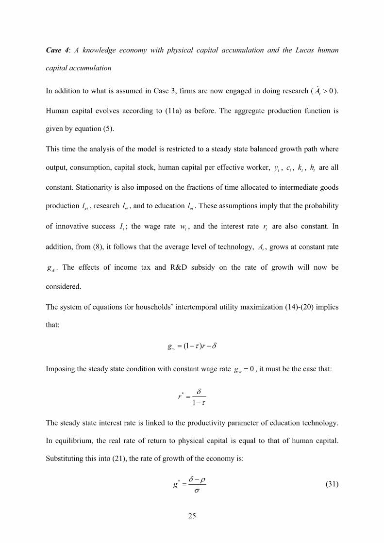
Equation (32) is the key result of the model; it contains all the necessary information about
the economy’s growth. It can be seen that the left hand side (which is denoted as ( )f g ), is a
decreasing function of g while the right hand side of the equation is simply a constant. In
addition, the investigation of limit gives:
lim ( ) 0g f g→∞ = , 0lim ( )g f g→ = ∞

28
Since 0Ω > , the solution to the above equation exists and is uniquely defined (single crossing
property). This is represented in Figure 1.
(Figure 1 here)
In principle, the above equation can be solved to get its closed form solution. It is inferred
from (32) that equilibrium growth is a function of parameters describing productivity of
education and research technology, consumers’ preferences, discount rate, and degree of
competition in the intermediate goods sector. However, because of the complication of the
procedures and the potential effects of all factors on its balanced growth path can still be
analysed, this paper keeps the solution implicitly instead.
The equilibrium interest rate and the fraction of human capital devoted to study will be:
**
1gr ρ στ
+=
−
**
*egl
gγ
ρ σ=
+
Proposition 2: Other things being constant, the steady state growth rate of the economy *g
increases with the education technology parameter δ , the R&D productivity λ , and the size
of quality increment µ .
Proof: To analyse the effects of all relevant parameters on g , one can differentiate ( )f g
with respect to every parameter to find out their corresponding changes. However, a much
simpler way is to investigate equation (32) (with a note that its left hand side is negatively
dependent on g ), then allow a parameter to vary at a time while others remain constant. As
an example, it can be seen that ( )f g is increasing in δ . An increase in δ makes the value of
( )f g higher. To keep ( )f g constant (equal to 1 according to (32)), it is necessary that g be

29
higher (as ( )f g is decreasing in g ). Similarly, one can do comparative statics for other
parameters of the model such as λ and µ . The effects are as described in Proposition 2
above.
The results obtained are similar to those of Aghion and Howitt (1998), Howitt (1999), and
Zeng (1997, 2002) although this paper is studied in a more comprehensive context. That
implies that human capital acquisition and innovations are two major driving forces of an
economy’s long-run growth.
Proposition 3: The size of population exerts no growth effect but it has a level effect.
Proof: It can be seen that the growth equation (32) does not depend on L explicitly. It means
the size of population has no effect on the long-run rate of growth of an economy.
This is a distinct feature that distinguishes the presented model from others because the scale
effect of population size is a common result of several endogenous R&D-based growth
models. Examples can be cited to Romer (1990), Grossman and Helpman (1991), Smulders
and van de Klundert (1995), and Perreto (1999). However, the result of this paper is not
subject to scale effect. This is apparent from research equation (8) which is based on the key
assumption that there are diminishing returns in the production of knowledge and constant
returns to human capital. An increase in L does not change the amount of human capital
devoted to research. With the introduction of human capital accumulation, growth will be
determined endogenously and scale effect is eliminated.
Nevertheless, population size does have level effect. From equation (6), given that xl , k , and
h are all constant in steady state, an increase in L will make the level of output per effective
worker y become lower. When the number of people increases, this also raises the “quantity”
of effective workers. Given that in steady state, output grows at the same rate as technology, it
ultimately lowers the average output per effective worker.

30
Proposition 4: When income tax is used to finance R&D subsidies, both tax and subsidy
affect the pace of growth of the economy. Moreover, there always exists a tax rate
* 20 1τ α≤ < − (and subsequently an R&D subsidy rate, *s ) that maximizes the long-run
growth.
Proof: The proof of the first part is presented here while the proof of the second part is given
in Appendix 2.
After dividing both sides by tA L and imposing the steady state condition, equation (23) for
the government budget constraint is equivalent to:
(1 )e rrk w l h swl hτ τ+ − =
This combining with (4) and (25) gives:
21s τ
α=
− (33)
This equation describes the relationship between R&D subsidy rate, s , and tax rate, τ , where
s is increasing in τ . This means that when the tax rate is higher, there will be more to
finance R&D expenditure, and the subsidy rate will be higher. Assume 0 1s≤ ≤ then it
follows from (33) that 2(1 )τ α− ≥ .
Substituting into the left hand side of equation (58), the new equilibrium equation is:
[ ]
(1 )(1 )1
(1 )(1 )(1 ) 1
12
1 11 11
1g g
γ χ ααβ
α γ χγ χ αβαβτρ σ τ α
τ µ
− − −−
− − −− − −−
− Γ = + − − + −
(34)
where
( )(1 ) (1 )(1 ) 211 1 11 2 11 21g g gg
αβ γ χ χχ γ χ ααβδγ ρ σ γ αγ χ χ χ αβµ λ αχρ σ ρ σ γ γ α β
− − − − −− − −− − −Γ = + ∆ −+ + −

31
and [ ](1 )1
2 21 111 . (1 ) (1 )
α β αβααβ αβαβ
γ χ µλα α α β α βγ
−−− −−
− − ∆ = − − as above.
This equation says that the income tax, and hence R&D subsidy, affects the growth rate. This
is in sharp contrast with the findings of Jones (1995a, b) and Arnold (1998) where they
conclude that those factors, representing for government intervention, are invariant to growth.
This is also different from results of Aghion and Howitt (1998) and Howitt (1999) in which
they (without considering tax) call for raising R&D subsidy in favour of growth. This model
investigates both tax and subsidy through their link in a balanced budget policy. A change in
tax affects interest rate as well as the allocation of human capital among different activities
which in turn affects every sector of the economy. In addition, a change in tax also leads to a
necessary change in subsidy to R&D activities through equation (33) which then has direct
effect on research sector. As a result, government intervention must have some role towards
growth. More specifically, the government can promote the economy’s growth by setting a
growth maximizing tax rate (and subsequently growth maximizing R&D subsidy rate) within
the interval 2[0,1 )α− .
5- Conclusions
This paper examines a Schumpeterian growth model in which physical capital accumulation,
human capital accumulation, and innovations are all considered in a growth process. The
paper distinguishes human capital from knowledge. While human capital is embodied in
people and is acquired through education, knowledge is embedded in objects or artefacts.
They are two complementary factors interacting with each other: human capital is employed
to produce knowledge through R&D and people study knowledge to absorb it and enhance
their stock of human capital. Physical capital that is accumulated from final output and
utilized to produce intermediate inputs is also introduced into the production of human
capital. In the economy human capital plays a role as an important input in most economic

32
sectors (except in the production of final consumption good). The paper investigates different
economic situations in which economies have different rates of growth. Following Funke and
Strulik (2000), it then goes on to discuss the general factor that influences the countries’ long-
run growth. In addition, it also looks at the effects of such policy variables as taxes and
subsidies on output growth.
The results of the system, viewed as a single and closed economy with no population growth
can be summarized as follows. Economies will see themselves in one of the economic
situations at which they enjoy different rates of growth. In the first situation, only physical
capital is accumulated and the representative economy has stagnant growth in output per
capita. Zero growth is also the result of a knowledge economy that is not accumulating human
capital. When economies start accumulating human capital, long-run growth is generated.
However, a balanced growth is only obtained when knowledge production is also in place.
When human capital is the only input in its own production as in Lucas (1988), the growth
rate only depends on parameters describing preferences and the efficiency of education
technology. It is completely invariant to R&D and policy factors. Nevertheless, when
education production takes knowledge and financial investment as two other inputs, long-run
balanced growth is driven by R&D technology, government fiscal policy as well as the degree
of competition in the intermediate goods sector. The paper highlights that education and
training and R&D activities are both important for growth. Government intervention, through
having a good fiscal policy, is also necessary for promoting growth.
The model considered in this paper is very general and comprehensive in the sense that it
encompasses different theories on growth in an integrated model. However, in the light of
these results, there are still questions open for future research. First, it will be interesting to
make a thorough empirical test on the influence of financial investment in human capital and
the level of competition on growth and the inter-sectoral allocation of skilled workers in the

33
economy. Second, in terms of expanding the theory, one possibility is to include physical
investment in R&D activities as it is believed that physical investment is also an essential
factor for doing research. Beside that, the second kind of R&D named horizontal innovations
is also worth investigating to enrich the literature.

34
Appendix 1
Derivation of the equilibrium growth condition for knowledge economy
Using the profit function (7) and imposing the steady state condition, the value of an
innovation can be calculated as the following:
(1 ) tt
A LyVr I
α α−=
+
Therefore, the arbitrage condition for innovations (9) now becomes:
(1 )(1 )( )
Lyws r I
µλα α−=
− +
In steady state, c , h , and e are constant so 0tc = and H E C K Yg g g g g g= = = = = . As a
result, equations (21) and (22) imply that:
1gr ρ σ
τ+
=−
(*)
(1 )egl
rγτ
=−
(**)
In addition, equation (4) gives:
2 (1 )x
yl hw
α β−=
2 ykr
α β=
Substituting these results into equation (6) we obtain:
(1 )2 21 (1 )y yy L
w r
α β αβα α β α β
−
− −=
or

35
(1 )2 21 11 (1 ).y
L w r
α β αβα αα β α β−− − −
=
Plugging this into the equilibrium arbitrage equation for the wage rate above we have:
(1 )2 21 1(1 ) (1 ).
(1 )( )w
s r I w r
α β αβα αµλα α α β α β−− − − −
= − +
Simplifying this expression gives:
[ ]1 1
(1 )11 1 1 2 21 111 1 1 (1 ) (1 )
1w
r I r s
α αβ αα β αβααβ αβ αβ
αβ αβαβµλα α α β α β− −
−−− − −− −−
= − − + −
In addition, the system of equations (14)-(20) implies the following:
.1 (1 )
tt
et t
Ewl H
γγ χ τ
=− − −
Hence:
1 11 1 11 1 1 1.(1 ) (1 ).
1t
e t
E wl H r I r s
α αβ ααβ αβ αβγ χ τ τ
γ
− −− − −− − = − = − ∆ + −
(A1.1)
where [ ](1 )1
2 21 111 . (1 ) (1 )
α β αβααβ αβαβ
γ χ µλα α α β α βγ
−−− −−
− − ∆ = − − .
By dividing both the numerator and the denominator of the left hand side of the above
equation by tA L , the relation in steady state is:
t
e t e
E el H l h
=
As a result, it delivers:
te
e t
Ee l hl H
= (A1.2)
From the equation describing R&D progress (8), we get:

36
t tA r r r
t t
H Hg g l l L l hLA A L
µλ µλ µλ= = = =
or
rgl h
Lµλ= (A1.3)
Therefore, together with (25), this implies:
2
2
1. . .1 1
e ee r
r e
l lgl h l hl L l
α βµλ α
−= =
− − (A1.4)
Equation (13), imposing the steady state condition that 0th = , delivers:
11t
ee t
El e gl H L
γχ
χδ−
− =
Using (A1.2), this implies that:
( )1
1te e
e t
El l h gl H L
γ χχ
χδ− −
− =
Now using (A1.1) and (A1.4), this becomes:
(1 )(1 ) (1 )1 1 11 1 1 e
ee
ll gr I r g l
γ χ α αβ γ χ χαβ αβ
χδ− − − − −
− − − Ω = +
where ( )(1 )(1 )
211 12
1 111 1s
γ χ α χαβγ χ γ χ χ χατ µ λ
α β
− − −−− − − − − Ω = − ∆ − −
Plugging the equation (*) into this equation, then applying (8), (25), and (**) gives equation
(32) for the equilibrium growth condition.

37
Appendix 2
Proof of proposition 4
First, notice that 1τ = (100 percent tax rate) is not the growth maximizing tax rate as it makes
the left hand side (LHS) of equation (34) become zero while the right hand side (RHS) is
equal to 1. In addition, in order for equation (34) to be well defined, 21 τ α− > is required.
For simplicity of notation, let 1t τ= − and consider the LHS of equation (34) as a function of
t , that is:
( )*( ) ( ),f t f g t t= (A2.1)
Given [ ]0,1τ ∈ and 2(1 )τ α− > then 2( ,1]t α∈ . Equation (34) says that ( )f t is a continuous
function of t over that interval. The implicit function theorem implies that:
( ) ( )* **
*
( ), ( ),( ) . 0f g t t f g t tdf t g
dt g t t∂ ∂∂
= + =∂ ∂ ∂
(A2.2)
Hence:
( )*
*
*
'( )( ),
g f tt f g t t
g
∂=
∂ ∂−
∂
(A2.3)
where ( )*( ),
'( )f g t t
f tt
∂=
∂ represents the partial derivative of the function with respect to t .
Given that (.)f is decreasing in g as discussed previously, then ( )*
*
( ),0
f g t tg
∂− >
∂.
Therefore:
( )*
sgn sgn '( )g f tt
∂= ∂
(A2.4)

38
where sgn(.) is a sign function. A value *t that maximizes ( )f t also maximizes the optimal
rate of growth *g .
Generally, the rule of differentiation gives:
ln ( )'( ) . ( )f tf t f tt
∂=
∂ (A2.5)
( )22 2
2 2
'( )ln ( ) ln ( ) ln ( )''( ) . ( ) . '( ) . ( )( )
f tf t f t f tf t f t f t f tt t t f t
∂ ∂ ∂= + = +
∂ ∂ ∂ (A2.6)
After taking log of ( )f t and partially differentiating the log function with respect to t , it is
the case that:
ln ( ) 1 2 (1 ) 1. 21 ( )f t gt t g gt t
γ χ α α ααβ µ ρ σ α
∂ − − − − −= − − ∂ − + + −
(A2.7)
And
[ ] ( )2 2ln ( ) 1 2 (1 ) 1.2 2 2 21 2( )
f t gt t g gt t
γ χ α α ααβ µ ρ σ α
∂ − − − − − = − + + −∂ + + −
(A2.8)
Using (A2.5), (A2.7), and the LHS of (34):
2
2 2ln ( )'( ) ( ) 0t
f tf ft α
α α=
∂ = < ∂ (A2.9)
And
1
ln ( )'(1) (1) 0t
f tf ft =
∂ = > ∂ (A2.10)
(A2.5) and (A2.7) say that '( )f t is a continuous function of t over the interval 2( ,1]α . Hence
results (A2.9) and (A2.10) imply that '( )f t changes the sign at least once over that domain.
In other words, there is at least one value of t at which '( ) 0f t = .

39
Depending on the values of parameters in the model, the equation '( ) 0f t = may have a
unique solution or many solutions. If the solution *t is unique, the function ( )f t reaches its
minimum value at *t and its maximum value at some t between 2α and 1. This is
represented in the table below.
t 2α *t 1
'( )f t - 0 +
( )f t
Min
If the equation '( ) 0f t = has more than one solution, there will be at least one local maximum
and the value that maximizes the function will also be between 2α and 1.
t 2α 1t 2t 3t 1
'( )f t
- 0 + 0 - 0 +
( )f t
Min Max Min
In short, there always exists 2 1tα < ≤ that maximizes the rate of growth of the economy.
From the value of 2( ,1]t α∈ , the value of τ can be worked out through the relation 1 tτ = −
meaning the growth enhancing tax rate *τ lies within 2[0,1 )α− . After finding *τ , the growth
maximizing *s can also be pinned down through equation (33).

40
Appendix 3
Mathematical Notation
Y = Final output
Q = Fixed production factor
α = Elasticity of final goods production function with respect to intermediate input
i = Intermediate good index
t = Time
iA = Technology level attached to the latest version of good i
A = Economy’s average technology level
ix = Use of intermediate good i in final production
τ = Income tax rate
C = Total consumption
K = Total physical capital
E = Physical investment in education
ε = Elasticity of substitution
Yp =Price of final good
ip = Price of intermediate good i
H = Total stock of human capital
xH = Human capital used in intermediate sector
rH = Human capital used in research sector
eH = Human capital used in education
β = Elasticity of intermediate goods production function with respect to physical capital
L = Size of population
k = Physical capital per effective worker
h = Human capital per effective worker

41
y = Output per effective worker
c = Consumption per effective worker
e = Investment in education per effective worker
xl = Fraction of human capital used for intermediate goods production
rl = Fraction of human capital used for research
el = Fraction of human capital used for education
π = Flow of operating profit for each intermediate firm
λ = Technical efficiency of research sector
µ = Magnitude of quality increment
I = Probability of innovative success
s = R&D subsidy rate
w = Wage rate paid to human capital
V = Value of a vertical innovation
mg = Rate of growth of variable m
δ = Efficiency of education
χ = Elasticity of education with respect to knowledge
γ = Elasticity of education with respect to human capital
a = Total asset holdings
ρ = Rate of time preference
σ = Coefficient of relative risk aversion
r = Interest rate paid to physical capital
H = Hamiltonian
λ = Costate variable
1 (1 )1A A Hα α β− −=
12A A α−=

42
References
Acermoglu, D., P. Aghion, and F. Zilibotti (2002), “Distance to frontier, selection, and
economic growth”, NBER Working Paper 9066.
Aghion, P. and P. Howitt (1992), “A model of growth through creative destruction”,
Econometrica, Vol. 60(2), 323-351.
Aghion, P. and P. Howitt (1998a), “Endogenous Growth Theory”, MIT Press.
Aghion, P. and P. Howitt (1998b), “Market structure and the growth process”, Review of
Economic Dynamics, Vol. 1, 276-305.
Aghion, P., M. Dewatripont, and P. Rey (1999), “Competition, financial discipline and
growth”, The Review of Economic Studies, Vol. 66(4), 825-852.
Arnold, L. (1998), “Growth, welfare, and trade in an integrated model of human capital
accumulation and research”, Journal of Macroeconomics, Vol. 20(1), 81-105.
Arrow, K. J. (1962), “Economic welfare and the allocation of resources for invention” in The
rate and direction of inventive activity: economic and social factors, a report of the
National Bureau of Economic Research.
Barro, R. and X. Sala-i-Martin (1995), “Economic Growth”, Mc Graw-Hill.
Blackburn, K., V. Hung, and A. Pozzolo (2000), “Research, development and human
capital accumulation”, Journal of Macroeconomics, Vol. 22(2), 189-206.
Blanchard, O. and S. Fischer (1990), “Lectures on Macroeconomics”, MIT Press.
Bond, E., P. Wang, and C. Yip (1996), “A general two-sector model of endogenous growth
with human and physical capital: balanced growth and transitional dynamics”, Journal
of Economic Theory, Vol. 68, 149-173.
Bucci, A. (2003), “R&D, imperfect competition and growth with human capital
accumulation”, Scandinavian Journal of Political Economy, Vol. 50(4), 417-439.

43
Dalgaard, J. and C. Kreiner (2001), “Is declining productivity inevitable?”, Journal of
Economic Growth, Vol. 6, 187-203.
De La Fuente, A. (2000), “Mathematical methods and models for economists”, Cambridge
University Press.
Funke, M. and H. Strulik (2000), “On endogenous growth with physical capital, human
capital and product variety”, European Economic Review, Vol. 44, 491-515.
Grossman, G. and E. Helpman (1991), “Innovation and growth in the global economy”, The
MIT Press.
Howitt, P. (1999), “Steady endogenous growth with population and R&D inputs growing”,
The Journal of Political Economy, Vol. 107(4), 715-730.
Howitt, P. and P. Aghion (1998), “Capital accumulation and innovation as complementary
factors in long-run growth”, Journal of Economic Growth, Vol. 3, 111-130.
Jones, C. (1995a), “Time series tests of endogenous growth models”, The Quarterly Journal
of Economics, Vol. 110(2), 495-525.
Jones, C. (1995b), “R&D-based models of economic growth”, The Journal of Political
Economy, Vol. 103(4), 759-784.
Jones, C. (2002), “Sources of US economic growth in a world of ideas”, The American
Economic Review, Vol. 92(1), 220-239.
Keely, L. (2002), “Pursuing problems in growth”, Journal of Economic Growth, Vol. 7(3),
283-308.
Leonard, D. and N. V. Long (1992), “Optimal control theory and static optimization in
economics”, Cambridge University Press.
Lerner, A.P. (1934), “The concept of monopoly and the measurement of monopoly power”,
Review of Economic Studies, Vol. 1(3), 157-175.

44
Lucas, R. (1998), “On the mechanics of economic development”, Journal of Monetary
Economics, Vol. 22, 3-42.
Peretto, P. (1999), “Firm size, rivalry and the extent of the market in endogenous
technological change, European Economic Review, Vol. 43, 1747-1773.
Romer, D. (2001), “Advanced macroeconomics”, second edition, McGraw-Hill.
Romer, P. (1986), “Increasing Returns and long-run growth”, The Journal of Political
Economy, Vol. 94(5), 1002-1037.
Romer, P. (1990), “Endogenous technological change”, The Journal of Political Economy,
Vol. 98(5), S71-S102.
Segerstrom, P. (1991), “Endogenous growth without scale effects”, The American Economic
Review, Vol. 99(4), 1290-1310.
Smulders, S. and T. van de Klundert (1995), “Imperfect competition, concentration and
growth with firm-specific R&D, European Economic Review, Vol. 39, 139-160.
Stokey, N. and S. Rebelo (1995), “Growth effects of flat-rate taxes”, Journal of Political
Economy, Vol. 103(3), 519-550.
Strulik, H. (2005), “The role of human capital and population growth in R&D-based models
of economic growth”, Review of International Economics, Vol. 13(1), 129-145.
Zeng, J. (1997), “Physical and human capital accumulation, R&D and economic growth”,
Southern Economic Journal, Vol. 63(4), 1023-1038.
Zeng, J. (2002), “Re-examining the interaction between innovation and capital
accumulation”, unpublished, National University of Singapore.

45
Figure 1- The steady state equilibrium growth rate
1
0 g
( )f g
*g
( )f g