Embed Size (px)
Citation preview

The role ofirrigation drains innutrient scavenging
Final Report NRMS Project M3105
CSIRO Land and Water Technical Report 26/98December 1998
C S I R O L A N D and WAT E R

Role of irrigation drainsin nutrient scavenging
Final Report on NRMS Project M3105Final Report on NRMS Project M3105
Jane Roberts, Martin Jane Roberts, Martin Thomas & Thomas & Shaun MeredithShaun Meredith
CSIRO Land and Water, CanberraCSIRO Land and Water, Canberra
December 1998December 1998

CitatioCitationRoberts, J. , Thomas, M. and Meredith, S. (1998) Role of irrigation drains in nutrientscavenging. Technical Report 26/98. CSIRO Land and Water. December 1998.
Final Report on NRMS Project M3105The full title of this project is: “The role of irrigation drains in nutrient scavenging: aproposal in botanical engineering”. Funded by the Murray-Darling Basin Commissionthrough its Natural Resources Management Strategy.
Cover PhotographThe cover photograph shows DC-S (Drainage Channel S) south of Griffith, in theMirrool Irrigation Area, and was taken on 9th February 1995. The water is clear, withfilamentous algae on the bottom sediment. The dense littoral vegetation is dominatedby floating mats of water couch Paspalum distichum, and by emergent macrophytes,mainly Schoenoplectus validus.
Disclaimer
CSIRO accepts no responsibility for anyinterpretation, opinion or conclusion that
any person may form as a result ofreading this report

i
Table of ContentsTable of ContentsTable of ContentsTable of Contents ii
AcknowledgmentsAcknowledgments viivii
Executive SummaryExecutive Summary viiiviii
Chapter 1 Project M3105Chapter 1 Project M3105 11
1.1 Nutrients as a cause for concern 11.2 Vegetated drains: The feasibility study 21.3 Project M3105 3
Scope of projectSocio-political contextDefining the approachHistorical perspectiveThree principlesProject organisation
1.4 The Mirrool Irrigation Area 5Drains and drainage waterYoogali gaugeMain Drain JWeather
1.5 Waterplants 7Weeds in Mirrool IA
1.6 Drain diversity 8References 8
Table 1.1 Weather summaryTable 1.2 Common weeds in irrigation drains in the MDBFigure 1.1 Location of study areasFigure 1.2 Seasonal flow regime at Yoogali gaugeFigure 1.3 Variable flow at Yoogali gauge: selected years
Photo EssayPhoto Essay 1515
Drains 16Drains During Winter 17Vegetation 18Western Australia – February 1994 19
Chapter 2 Classifying Drains for Ecological PurposesChapter 2 Classifying Drains for Ecological Purposes 2020
2.1 Working in constructed environments 20Drain classificationConstructed and natural systems

ii
Stream orderObjectives
2.2 Methods 22Ordering and catchmentsCatchment characteristicsAnalysis of results
2.3 Results 25Pilot studyThe Mirrool studyBasin applicationCatchment analysis
2.4 Discussion 28Findings
References 29
Table 2.1 Pilot study: Channel dimensionsTable 2.2 Mirrool study: CatchmentTable 2.3 Mirrool study: Drain dimensionsTable 2.4 Mirrool study: Within drain attributesTable 2.5 Mirrool study: Chemical characteristicsTable 2.6 Mirrool study: Vegetation coverTable 2.7 Basin application: Site detailsTable 2.8 Basin application: Channel dimensionsTable 2.9 Basin application: VegetationTable 2.10 Catchment analysis for Coleambally IAFigure 2.1 Pilot study: Stream orders in Hanwood sub-catchmentFigure 2.2 Mirrool studyFigure 2.3 Pilot study: Vegetation coverFigure 2.4 Pilot study: Vegetation cover based on life historyFigure 2.5 Mirrool study: Drain dimensionsFigure 2.6 Mirrool study: Incidence of zero flows
Chapter 3 The Trunks and Tribs Study: Lateral DrainsChapter 3 The Trunks and Tribs Study: Lateral Drains 4141
3.1 Targeting the hot-spots 41Objectives
3.2 Methods 42Study areaSite set upField study and samplingData presentation and analysis
3.3 Results 453.4 Discussion 48
Identifying low-flow hot-spotsFindings and conclusionsMacrophyte location
References 51

iii
Table 3.1 Sampling sitesTable 3.2 Tributary low-flowsTable 3.3 Frequency of zero flows by land use typeTable 3.4 Water quality for individual drainsTable 3.5 Land use and water quality signaturesTable 3.6 Low-flow loads in individual drainsTable 3.7 High exporting drainsFigure 3.1 Sampling sites for Trunks and Tribs studyFigure 3.2 Flows in 24 tributary drainsFigure 3.3 Seasonal trends in water qualityFigure 3.4 Tributary water quality: Seasonal patterns by land useFigure 3.5 Seasonal loads for types of land use
Chapter 4 High Flows and Rainfall EventsChapter 4 High Flows and Rainfall Events 6464
4.1 Rain, high flows and water quality 64Pathways to irrigation drainsCrop type, stage and drainage dischargeRun-off calendarAims and objectives
4.2 Methods 67Hydrograph comparisonsWater quality monitoring and comparison
4.3 Results 69Hydrograph comparisonWater quality comparisonEvent 1 18th and 19th January 1994Event 2 11 July 1994Event 3 17th-18th May 1995All Events
4.4 Discussion 72Rainfall and dischargeWater quality variabilityFindings
References 75
Table 4.1 Sampling details for comparison of hydrographsTable 4.2 Sampling details for three eventsTable 4.3 Summary of rainfall - discharge responsesTable 4.4 All events: range in water qualityFigure 4.1 Seasonal patterns in discharge responses to rainfallFigure 4.2 Event One: Background variability: mid-summerFigure 4.3 Event Two: Winter: 11th July 1994Figure 4.4 Event Three: Water Quality: 17-18 May 1995
Chapter 5 Trunks and Tribs Study: Main Drain JChapter 5 Trunks and Tribs Study: Main Drain J 8484
5.1 Water quality in exit drains 84Monitoring

iv
Within-drain processesNutrient yield from sub-catchmentsObjectives
5.2 Methods 85Within-drain processesNutrient yields
5.3 Results 87Main Drain JWater quality - concentrationsWater quality loadsWithin-drain processesNutrient yields
5.4 Discussion 90Conclusions and findings
References 91
Table 5.1 Land uses within eastern Mirrool area, 1994-1995Table 5.2 Occurrence of high rainfalls by monthTable 5.3 Loads and seasonal comparisons in Main Drain JTable 5.4 Nutrient yieldsFigure 5.1 Velocity in Main Drain JFigure 5.2 Seasonal patterns of low-flows in Main Drain JFigure 5.3 Water quality changes in Main Drain JFigure 5.4 Seasonal loads in Main Drain JFigure 5.5 Load changes within Main Drain JFigure 5.6 Nutrient yields by land use
Chapter 6 Sediments and BioturbationChapter 6 Sediments and Bioturbation 101101
6.1 Sediments and bioturbation 101Bioturbation and CarpObjectivesSedimentsBioturbation
6.2 Methods 103Distribution patterns of sedimentary TP in lateral drainsLongitudinal changes in an exit drainBenthic macro-invertebratesNutrient sediment surveyFecal contaminationBioturbationCarp distribution and abundanceSediment and phosphorus resuspension
6.3 Results 106Sediment characteristicsDistribution patterns of sedimentary TP in lateral drainsLongitudinal changes in an exit drainMacro-invertebrates in Main Drain JNutrient Sediment SurveyFecal contamination
v
BioturbationCarp distribution and abundanceSediment and phosphorus resuspension
6.4 Discussion 109Sediment quality and compositionCarp: Distribution and abundanceEvaluation of bioturbation by carpConclusions and findings
References 112
Table 6.1 Variation in TP concentrations in Mirrool Irrigation AreaTable 6.2 Chemical composition of sedimentsTable 6.3 Benthic macro-invertebrates in Mirrool Irrigation AreaTable 6.4 Nutrients in sedimentsTable 6.5 Carp abundance in drains of Mirrool Irrigation AreaTable 6.6 Characteristics of sediments used in re-suspension experimentTable 6.7 Effects of carp on selected aspects of water qualityFigure 6.1 Carp feedingFigure 6.2 Sediment surveyFigure 6.3 Carp observation sitesFigure 6.4 Sediment TP in Main Drain JFigure 6.5 Characteristics of Main Drain J
Chapter 7 Whitton DrainChapter 7 Whitton Drain 122122
7.1 Macrophytes, drains and water quality 122Objectives
7.2 Materials and methods 123Site descriptionField samplingData preparation and analyses
7.3 Results 126General observationsNutrient concentrationsVegetation surveysDrain sectionsChanges in water quality
7.4 Discussion 130Micro-processesFindings
References 134
Table 7.1 In-flows to the Whitton study drainTable 7.2 Growth-forms of plants recorded in Whitton DrainTable 7.3 Changes in vegetation January to MarchTable 7.4 Ecological zones in Whitton DrainTable 7.5 Changes in nutrient loads: between sitesTable 7.6 Changes in nutrient concentrations: between sitesFigure 7.1 Whitton Drain

vi
Figure 7.2 Velocity and discharge in Whitton DrainFigure 7.3 Aquatic environment in Whitton Drain, summer 1994Figure 7.4 Water quality in Whitton DrainFigure 7.5 Water quality in Whitton DrainFigure 7.6 Vegetation in Whitton Drain in January 1994Figure 7.7 Vegetation changes February to MarchFigure 7.8 Effect of velocity on change in TP load
Chapter 8 Synthesis and FindingsChapter 8 Synthesis and Findings 146146
Stream ordering and drain classification 146Effectiveness of vegetated drains 147Locating the treatment process 148
Exit drains as plant habitatsDrain selection and implementationPhragmites australis and Paspalum distichum
Getting the target right 150Defining the location of the water quality problemDefining the type of water quality problemSource material on irrigation drains
Conclusion 152References 15 2
Table 8.1 Drains as macrophyte habitatTable 8.2 Characteristics of drains across the Basin
AppendAppendix A The Brief 156
Appendix B Activities relating to M3105Appendix B Activities relating to M3105 159
Appendix C Abstract of MSc thesisAppendix C Abstract of MSc thesis 162
Appendix D Standard Procedures and MethodsAppendix D Standard Procedures and Methods 164
Appendix E Water Quality in Mirrool IAAppendix E Water Quality in Mirrool IA 168

vii
AcknowledgementsAcknowledgements
An applied research project such as this benefits enormously from the goodwill andco-operation of organisations and individuals. We would like to thank thefollowing:
The NSW Department of Water Resources / Department of Land and WaterConservation for assistance with data, and answering queries: in particular AlistairBuchan, officers at the Tumut office.
Murray-Darling Basin Commission for their support and patience with re-focusingthe brief, in particular Bob Banens and Michael Htun.
Murrumbidgee Irrigation for assistance with enquiries re data, procedures andproviding background understanding: n particular, Graham Carter, Lillian Parker,Pat Spence, Douglas Graham, Jim Neville and Les Ellis.
Griffith laboratory of CSIRO Water Resources / Land and Water. Alan Chick, andAndrew Palmer for help in the field; Vicki Patten, Peter Thompson, Sharyn Fosterand Wendy Minato for prompt chemical analysis; Geoff McCorkelle for help in thefield, photomosaics and helpful discussions; Clare Bowditch in the administrationarea; Dr Liz Humphreys and Geoff McCorkelle for explaining aspects of irrigatedagriculture; and Dr Richard Davis (Canberra) for supporting this project.
Students and casual employees Nikki Ward, Simone Rolfe, Amy McCudden andShaun Meredith for their effective contributions.
Co-supervisers, advisers and helpers of post-graduate students: Dr Laurie Olive,ADFA University of New South Wales, Dr Keith Walker, University of Adelaide;Geoff Sainty, Sainty and Associates; Dr Peter Fairweather, Deakin University,Warrnambool.
A special mention for the following individuals:
♦ Warren Muirhead and Lillian Parker, for helpful criticism and comments
♦ Peter Randell, Murrami, for showing drains on an organic farm
♦ Dr Kath Bowmer, Charles Sturt University, for anticipating the need for thiswork, and for setting up this project.

viii
Executive SummaryExecutive Summary
BackgroundBackgroundNutrient loads in rivers have been a management concern since the spectacular algalbloom on the Darling River in 1991. A modelling study completed in 1992 identifiedirrigation areas as one of two major point-sources of nutrients reaching the Murray-Darling river system. A subsequent review of the data on irrigation water qualityfound major data and knowledge gaps and recommended a range of strategies toreduce nutrient loads leaving irrigation areas, including in situ treatment by drainvegetation.
The effectiveness of this was then investigated in a short-term feasibility study, doneon irrigation drains near Griffith, New South Wales. This found that concentrationsof some nutrients (turbidity, TP and FRP) were reduced by passage down a ‘weedy’drain and concluded that the prospects for in situ treatment of nutrients werepromising. This project builds on the earlier feasibility study, extending it andaddressing the questions raised.
ObjectivesObjectivesThe overall aim was to assess the prospects for using irrigation drains in theMurray-Darling Basin to improve water quality by maintaining the in-drain aquaticplant (weed) communities. Questions nested within this were; land use effects;high flows; the importance of bioturbation; selection of target plant species;sources and sinks of nutrients; differences between main drains and lateral ones.
A secondary aim was to develop a drain classification system, in order to develop asummary description of drains as aquatic habitats. For this, ideas and techniqueswere ‘borrowed’ from stream hydrology. Catchment analysis was trialled as ameans of describing irrigation areas and stream ordering for classifying irrigationdrains.
Water quality as used in this report refers to concentrations and loads of nutrients,nitrogen and phosphorus, and suspended sediments.
ActivitiesActivitiesA series of field investigations was done in drains, mainly in the Mirrool IrrigationArea (Mirrool IA) near Griffith in southern New South Wales, as follows:
Drain classification was explored by applying an extrinsic method of classification,stream ordering, to drains locally, regionally and then across southern part of theBasin, and assessing the results. The ‘Trunks and Tribs’ study was an investigationspecific to low-flow conditions, of seasonal patterns in water quality in lateral drains,and the role of land use in determining water quality characteristics and nutrientyields. In addition, the sources and sinks of nutrients in the main exit drain weredetermined by preparing a low-flow nutrient budget for each month from Octoberto June. High flows were investigated separately in the Events study, which usedintensive monitoring to document water quality changes and reported on seasonaldifferences in the effect of rain on discharge. In the Bioturbation study, thesignificance of benthic feeding behaviour of carp was assessed by field monitoringand experimentation. Finally, in the Whitton study, changes in water quality down

ix
a vegetated stream order one drain, such as might be utilised for water qualityimprovement, were linked to plant abundance.
Other activities included telephone survey of practices and information acrossirrigation areas; and the appointment of two post-graduate students, oneresearching bioturbation by carp Cyprinus carpio L., and one researching drainclassification and catchment analysis.
FindingsFindings
Drain classificationDrain classificationStream order is a standard and widely-used means of describing and classifyingsections of rivers. The Strahler system proved effective as a means of classifyingdrains into broad physical types, and in summarising downstream changes inphysical characteristics of drains. It was not effective in summarising chemical orvegetation responses. For chemical characteristics, stream order must be used inconjunction with dominant land use. Plant abundance, as cover, was not well linkedto stream order or water quality. This was attributed to effective weed managementprograms across the Basin. Drain classification could be further refined by includingcatchment size, soil types and slope.
The range of stream orders for irrigation drains is limited, relative to river systems.Even in large irrigation areas such as Mirrool Irrigation Area in New South Wales,drains were mainly stream order one, two and three (SO1 to SO3). The main exitdrain, Main Drain J, was an order four (SO4).
Stream ordering and dominant land use were useful in summarising drains withinan irrigation area, and allowed comparison between irrigation areas. A comparisonbetween seven irrigation areas showed that drains, as aquatic environments, are notuniform across the Murray-Darling Basin. Even drains of same stream order andsimilar land use have different physical and chemical characteristics.
Irrigation areas as catchmentsIrrigation areas as catchmentsStandard techniques for describing catchments can be applied to sub-catchmentswithin irrigation areas, or to whole irrigation areas.
Targetting the right drainsTargetting the right drainsIdentifying drains for nutrient treatment means identifying where nutrients arehighest. The location of nutrient hot-spots, if not already known through waterquality monitoring programs, can be approximately identified using indirectindicators.
Indirect indicators investigated in the Mirrool Irrigation Area were land use anddischarge, exclusive of rain-stimulated discharge. There was a strong link betweenland use and water quality (concentration) in lateral drains. Broadacre andhorticulture sub-catchments produced drainage with distinctive signatures, that isthey each had a characteristic range of water quality concentrations. In contrast, thelink between land use and water quality (loads exported) was not strong and loadswere determined by discharge, even under low-flow conditions. Drains whichcontributed highest loads to the main exit drain tended to be those with the highestmedian discharge.

x
No drain was identified which provided an environment ideal for in situ waterquality improvement.
The most suitable drains were laterals, particularly SO1 and SO2 ones, rather thanSO3 and main exit drains. In the Mirrool Irrigation Area, small lateral drains aremore favourable for plant growth because the water is not as deep, or as turbid andflows more slowly than in the main exit drain.
Diagnosing the water quality problemDiagnosing the water quality problemResolving the nature of the water quality problem is necessary as this determinesthe course of action for each management area. Questions to be resolved areconfirming that nutrients are a water quality issue; and if so, then whether thetarget is reduction of nutrient concentrations or loads.
In Mirrool IA, nutrients were not the main water quality issue in the upper reachesof Main Drain J. Median concentrations of TP, TN and NOx during low flows wererated Medium, following criteria used by Harrison (1994). Nutrient yields, as kg ofnitrogen or phosphorus per hectare during the irrigation season, were lower thanreported in the literature. However, suspended sediments appeared to be aproblem. Median SS concentration was double that recorded for the middle reachesof the River Murray, and yields of suspended sediment were 1-2 orders ofmagnitude higher than nutrient yields.
Carp are probably not a factor in phosphorus export, contrary to public anticipationthat their feeding behaviour re-suspends nutrient-rich sediment. The phosphoruscontent of drain sediment in Mirrool IA was not high relative to eutrophic systems,and was higher in drains with urban development in the catchment. The greatestabundances of carp were at the junction of lateral drains with main exit drain.
Lateral drains with the highest nutrient concentrations were not necessarily thedrains with the highest nutrient loads, even under low-flow conditions. Thus anutrient reduction strategy targetting concentrations will focus on different suite oflateral drains than a strategy focusing on nutrient loads.
Discharge had a dominating effect on nutrient load exported, hence a managementstrategy aiming at load reduction will have to focus on managing discharge. Inirrigation areas this includes how landholders and authority responds to rainfall.Recent changes requiring partial retention of run-off may already be having apositive effect.
Limitations and management issuesLimitations and management issuesDuring the Whitton study, extensive mortality of fish, macrophytes and possiblyalgae was noted and biocides were suspected. In addition, a critical velocity forsediment entrainment and deposition was empirically determined, and theimportance of silt beds with organic material for effecting nitrogen transformationswas inferred.
Using vegetation to improve water quality can only be effective if drains arespecifically managed and if specific management criteria are developed and adheredto. Such criteria would have to include zero discharge of agricultural chemicals ortheir breakdown products, persistent low flows and in particular low velocities, andreduced de-silting or a new de-silting / drain maintenance program.
xi
Overall prospectsOverall prospectsOverall, the prospects for using vegetation in drains to improve the quality ofirrigation drainage water are limited to a few drains, but in these this kind of in situtreatment could be a useful management option.
The most suitable drains are the smaller ones, usually stream order one and two.The most favourable time of year, ie when vegetation reaches highest biomass andtemperatures encourage microbial activity, is during summer and autumn. Themost effective conditions are when flows are low enough for deposition ofparticulates.
Opportunities are limited because not all drains provide growing conditions that aresuitable for plants, not all drains have discharge capacity necessary, only somedrains have flows that are low enough and the timing of low flows may berestricted. In addition, only two processes of nutrient removal are likely to beeffective: particulate deposition and denitrification.
RecommendationsRecommendationsDrain ClassificationDrain Classification
1 Stream order and land use can be used in combination as a basis for aphysical classification of irrigation drains and catchment attributes be used todescribe and summarise irrigation areas.
Water Quality and Water Quality and Ecological functioningEcological functioning
2 Rather than being removed, for example by de-silting, sediment depositsshould be viewed as potential denitrification sites. Some should be maintained, atleast temporarily and perhaps on a rotation system. These would need to bemanaged sympathetically to encourage microbial populations, for example byavoiding pesticide treatment in the vicinity or upstream.
3 Small lateral drains, particularly stream order one and two drains, are mostsuitable for managing as linear drainage treatment units.
4 The macrophyte cover on main Exit Drains is distinctive and its ecologicalsignificance for habitat and water quality needs to be evaluated.
5 Irrigation authorities interested in the application of in-stream water qualityimprovement need to recognise that specific identification of suitable drains willrequire the sympathetic collaboration and fusion of engineering, hydrologic andecological skills.
6 Species robust to conditions in irrigation drains include Phragmites australisand Paspalum distichum. These plants should be encouraged, where feasible, byreducing weed control programs and by stock exclusion.
7 Sources of nutrients in irrigation drains need to be specifically defined andthe relative importance of irrigated agriculture, domestic or urban, and industrialsources quantified.
8 Reasons for high sediment loads in Mirrool IA should be identified and costsof this evaluated.
9 An inventory of irrigation drains is needed for each management area withinthe Basin, giving status of whether open or closed (piped), construction details (age,method, material), sources of drainage (irrigation, urban, septic, stormwater) as wellas spatial information (length, position, discharge points).

1
Chapter 1Chapter 1
Project M3105Project M3105
1.11.1 Nutrients as a cause for concernNutrients as a cause for concernIn the early 1990s, the quality of water in inland rivers in the Murray-Darling Basin(henceforward the MDB or the Basin), and in particular the levels of nutrientsbecame a major concern. Managerial perception at that time was that “While algalblooms are not new to our inland rivers, there is little doubt that the frequency andintensity of these blooms is getting worse” (GHD 1992, p1).
In 1990, the Murray-Darling Basin Commission instigated a nutrient managementstrategy and commissioned Guttridge, Haskins & Davey (GHD) to review nutrientsources, data available and assess the importance of nutrients under differentcircumstances within the Basin. This was completed in January 1992. Nutrientmodelling (phosphorus) for three of the main rivers in the MDB showed thesignificance of flow. Nutrient loads were lowest in a dry year and highest in a wetyear, and point sources exceeded diffuse sources only in dry years. The pointsources considered were: municipal sewage treatment plants, industrial inputs,irrigation drainage, urban stormwater and intensive animal agriculture.
Irrigation drainage was identified as the second highest point source of nutrientpollution, with municipal sewage treatment plants being the highest. In an averageflow year, irrigation areas were estimated to be contributing 170 tonnes of totalphosphorus and 980 tonnes of total nitrogen to rivers in the Basin (GHD 1992). Twoirrigation areas, Sunraysia in Victoria and the Lower Murray in South Australia,were among the most significant for the main stem of the River Murray. Findingswere presented in broad terms as much of the data used in this preliminarymodelling was known to be “sparse or short term” (GHD 1992, p7-27).
At the time that this nutrient modelling was being completed (GHD 1992), one of thelargest and most extensive algal blooms ever reported occurred on the DarlingRiver, in November-December 1991 (Bowling and Baker 1996). The bloom wasdominated by the cyanobacterium Anabaena circinalis. Toxicity of the strains in theriver was patchy but ranged from zero, to moderate, and even high: stock deathsresulted. Nutrients were implicated as both total phosphorus and total nitrogenwere high (Bowling and Baker 1996) and hence the source of nutrients wasquestioned. The full complexity of blooms, the importance of flow as a determiningfactor and the relevance of sediment dynamics and catchment lithology were notappreciated until much later. An immediate consequence of Australia’s biggestalgal bloom was a heightened awareness in agencies, authorities, councils, privatetrusts and corporations charged with supplying water that their responsibilitiesincluded supply of safe water and its disposal. Hence high concentrations ofnutrients, usually meaning forms of nitrogen and phosphorus, were a problem.
In irrigation areas, this nutrient problem can be addressed by managing nutrients attheir source, for example by minimising nutrient run-off from farms (eg Neeson1996), by reducing other nutrient inputs, by diluting (this option assumesconcentration is the issue rather than load) or by treating drainage. Penalties and

2
regulations can be used to re-enforce any of the above, but are not in themselves anutrient management or reduction strategy.
The data on nutrients in irrigation drainage were considered by Harrison (1994).She collated and assessed data availability and quality, summarised broaddifferences in crops between states and between river valleys, and broadly relateddrainage water quality to crop type. Harrison (1994) was impressed by theinadequacy of the water quality information to hand. Coverage was uneven acrossthe Basin; there were gaps in the array of water quality parameters measured (mostnotable was organic nitrogen), a lack of contextual information including flow data,and the links between farm practice and drainage quality were not being made.
The report by Harrison did not change the findings made by GHD (1992) but insteadconfirmed them, at least in relation to irrigation, and placed them on a moresubstantial footing. Access to unpublished and in-progress data confirmed theimportance of irrigation drainage as a source of nutrients and emphasised the needfor active management (Harrison 1994). Better on-farm management was stronglyrecommended and research into various ways of treating drainage was called for,including vegetated drains, vegetated buffer strips, irrigated wood lots and re-useschemes.
1.21.2 Vegetated drainVegetated drainss: The feasibility study: The feasibility studyThe use of vegetated drains to improve water quality was the subject of a briefinvestigation “The effect of aquatic plants on water quality in irrigation drains: Afeasibility study for the Murray-Darling Basin Commission” (Bowmer et al. 1992,Bowmer et al. 1994). This study was nearly contemporary with Harrison’s review,and its outcomes were known to her.
The feasibility study was done in late summer, March-April 1992, near Griffith, NewSouth Wales. It considered suspended sediment in the main exit drain and itssource (this was because nutrients, especially phosphorus adsorb onto inorganic soilparticles). It also documented the effect of a tile drain input on water quality, andlooked at longitudinal changes in drainage water quality. The main findings were:
♦ Turbidity increased markedly down the main drainage channel as it passedthrough the irrigation area immediately south of Griffith. A turbidity (as NTU)budget on 19-20 March 1992 found no evidence to support the hypothesis thatturbidity was generated in situ by turbulent re-suspension or by erosion.
♦ Tile drain discharge into Western Drain on 18 March 1992 made little differencedownstream to discharge (a 4% increase) but substantially increased bothconcentration and load of total nitrogen (53% and 58% respectively), howeveroxidised nitrogen virtually disappeared.
♦ Concentrations of total phosphorus and filterable reactive phosphorus decreasedwhile passing through a ‘weedy’ section of two drains, Murrumbidgee AvenueDrain on 22 April 1992, and Drainage Channel-S (DC-S) on 4 dates in March1992.
♦ The effect of carp Cyprinus carpio was to increase turbidity in the ‘weed-free’sections of a lateral drain, as determined by upstream v downstreamobservations in de Bortoli’s Road drain on 31 March 1992, and confirmed in afield trial comparing before and after applying a herbicide (xylaquat, and toxic tocarp) to DC-S on 13 April 1992.

3
♦ No effect by plants on water quality was detected when nutrient concentrationswere very low.
♦ Suspended sediment concentration (as mg L-1) and turbidity (as NTU) werehighly correlated (r2 > 0.78 for each of 4 data sets) but the relationship changedbetween sites and times. Total phosphorus (TP) and turbidity (NTU) werepoorly correlated.
The feasibility study noted that there was an almost complete lack of knowledgeabout the effects of plants at different times of the year, and about the biology andbehaviour of carp in irrigation drains (Bowmer et al. 1992). It concluded that:
♦ Prospects for managing vegetation to trap suspended particulate load andnutrients, without sacrificing hydraulic performance for flood mitigation, were“good”.
♦ Water couch Paspalum distichum was identified as a “suitable robust species”.(Although water couch was recommended as a useful species, it occurred at onlyone of the five study sites).
Although these conclusions were generally positive, the study did point to majorgaps in knowledge. There was not enough known about the phenology of waterplants in drains. Even more significant, in the context of evaluating drains as ameans to improve water quality, was the lack of knowledge of drains as habitats forwater plants, and the range of conditions within a drainage system. The feasibilitystudy used only five irrigation drains near Griffith. These were chosen for theiraccessibility and the good opportunities (ie high vegetative cover) for scientificresearch. It was not known if these were representative of drains elsewhere. Inorder to place this research in context, the Murray-Darling Basin has approximately7900 km of irrigation drains (indicative estimate provided by Sandy Robinson,MDBC, pers. comm. 1998).
This feasibility study was one of the first investigations in Australia on nutrientinterception in lotic (flowing) vegetated systems. Nearly all other investigations intothe use of vegetated aquatic systems to improve water quality have been done inlentic (standing water) vegetated systems, such as constructed wetlands.
1.31.3 Project M310Project M31055
Scope of projectScope of project Because of the positive outcomes from the feasibility study, the Murray-DarlingBasin through its Natural Resources Management Strategy (NRMS) supported a 3-year study to continue research and application. The proposal was entitled: “Roleof irrigation drains in nutrient scavenging / biomanipulation: a proposal inbotanical engineering”. Water quality, as used here, refers to nutrient and sedimentloads, and does not include pesticides. A summary of pesticide research done byCSIRO in the MIA is available (Bowmer et al. 1998).
The aims and objectives of this 3-year project as outlined in the original application(Appendix A) were:
♦ Structural approach: to survey drain characteristics, and devise a classificationscheme
4
♦ Experimental investigations: to determine the factors mitigating theeffectiveness, or otherwise, of plant communities in drains in protecting waterquality; fate of nutrients within drains
♦ Extension: Preparation of a manual or handbook.
The number of experiments was subsequently reduced from more than six to three,in consultation with MDBC, and the advisory manual not implemented. Theconcept of a manual pre-supposes specific technical and positive outcomes.
Socio-political contextSocio-political contextWhen this research project began, the irrigation industry throughout the Basin wasgoing through major re-adjustment. Irrigation areas which had been government-run were being gradually corporatised or privatised. While this re-adjustment wasunderway, dealings with various sectors was not straightforward. Informationretrieval was sometimes improved, sometimes not. The result was that continuity ofknowledge was broken. Not all government staff were re-employed by the newcorporations, and those that were re-employed found themselves in organisationswith different management structures, different goals, and often with differentduties. On the positive side, resource descriptions were initiated, sometimes inanticipation of land and water management plans.
Defining the approachDefining the approachUsing aquatic plants in irrigation drains to improve the quality (specificallynutrients) of drainage water leaving an irrigation area is a soft or green approach. Ithas a certain appeal because it offers, or appears to offer, a low-cost, self-sustainingalternative to a highly engineered, physically-structured approach.
Historical perspectiveHistorical perspectiveFrom the 1900s until recently, that is for nearly the entire history of irrigation inAustralia, irrigation drains have been perceived as hydro-engineering structures,constructed to remove irrigation run-off, rainfall, tile-drain effluent and sometimesgroundwater.
In the 1990s, however, drains became more diverse and water increased in value.Drains now function as part of the supply system, a new role added to an existing,and often venerable, irrigation system. This is a dual function which can placestresses on the system’s physical structure and on its management. Multi-functioning of irrigation drains is beginning to be recognised. Issues such asdownstream water users, social responsibility and accountability, and water qualityin its broadest sense, not just salinity and turbidity, mean irrigation drains are nowreceiving the kind of attention formerly directed to rivers. At a conference atMoama, New South Wales in March 1997, the chairman said “... drains should nolonger be left to the responsibility of single professions” (Keyworth 1998). When thisproject began, the hydro-engineering perspective towards drains was still strong.
The ecology of drains has received almost no scientific attention in Australia, thusthere is thus no knowledge base for promoting an ecological perspective. There arevery few plant or animal studies, except for two on water rats (McNally 1960,Woollard et al. 1978). The brief essays by different contributors in Sainty and Jacobs(1990) is the only compilation published on drain ecology. In this it is apparent thatmost plants and animals are viewed negatively because they are thought to interfere

5
with drain performance. Thus water plants are ‘weeds’ because they reducehydraulic capacity; water rats and yabbies are pests because they puncture channelwalls by burrowing; and carp are a nuisance because they cause undermining,hence slumping and then bank erosion (Sainty and Jacobs 1990, Jackel 1996).
Three principlesThree principlesThree principles were adopted to guide this research:
Drain classification using simple data: Information to be used for drainclassification, description and comparison should be minimal but reliable or robust,and readily available. If not already available, then it should be easily obtained, andshould not require huge field effort to obtain. Simple data requirement does notmean simple environments.
Drainage networks are catchments: Irrigation areas are similar tocatchments, despite being constructed on the landscape. Although this is rarelyacknowledged, this determines sampling designs used in water quality monitoringprogram.
Drains are aquatic habitats: None of the studies on individual speciesaddressed the question of drains as a habitat. There is no interpretation of irrigationdrains as an ecological environment yet this is essential if an ecological approach todrain management is to work.
Project organisationProject organisationThis report presents research by topic and theme. Individual roles and contributionsare given below (Appendix A). Because of the location of the CSIRO laboratory nearGriffith, New South Wales, most of the field work for this project was centredaround Griffith in the Mirrool Irrigation Area (Mirrool IA). Work was extended toother irrigation areas where appropriate, and field trips and familiarisation visitsdone to broaden knowledge and understanding (Appendix B).
Methods used are described in the text for each chapter, except for water samplingand discharge. The standard procedures as used at the laboratory of CSIRO Landand Water (at the time CSIRO Division of Water Resources), including fieldprotocols, preparation and analytical procedures, are given below (Appendix D) andnot described in each chapter, unless radically modified. Henceforward thefollowing abbreviations are used: TP for total phosphorus, FRP for filterable reactivephosphorus, TN for total nitrogen, TKN for organic nitrogen as total Kjehldahlnitrogen, NOx for oxidised nitrogen (sum of nitrate and nitrite) and NH4 forammoniacal nitrogen, and SS for suspended sediments.
1.41.4 The Mirrool Irrigation AreaThe Mirrool Irrigation AreaThe Murrumbidgee Irrigation Areas (MIA) comprises the Mirrool and YancoIrrigation Areas, and the Tabbita, Wah Wah and Benerembah Irrigation Districts.Towns associated with the MIA are Griffith, a major regional centre, and Leeton.The MIA is one of the larger and older irrigation areas. Yanco and Mirrool wereestablished in 1912 and together comprise 163,550 ha of which 113,377 is irrigated(Crabb 1997). The Irrigation Districts were set up in the 1930s. A summary oninformation on age, size, and number of holdings in different irrigation areas in eachof four states is given by Crabb (1997).

6
Irrigated agriculture in the Mirrool IA is quite diverse. The main crops are citrus,wine grapes and rice, but there are also winter cereals, vegetables, soybeans, maize,sunflowers and stone fruit. The area under specific crops changes according tocommodity prices. In the last decade, the area under citrus has been contracting,while the holdings of wine grapes have been expanding. In 1996-1997, there were8908 ha of irrigated citrus, 9014 ha of wine grapes, 628 ha of irrigated stonefruit and38,926 ha of rice (Lillian Parker, Murrumbidgee Irrigation, pers. comm. 1998). TheMirrool IA is about three quarters of the MIA.
Hydrological modelling (BBSWAMP for the Land and Water Management Plan)suggests that annual diversions out of the Murrumbidgee River are 1080 GL, thoughthis is probably an overestimate. Most of the water diverted into the MIA comesfrom Berembed Weir, upstream of Narrandera, into the Main Canal and on to theMIA. The Main Canal, which is 160 km long, is the main irrigation and domesticwater supply for Griffith and Mirrool IA. The Sturt Canal, near Gogeldrie Weir, alsodiverts water from the Murrumbidgee River into the MIA. Flow rate out of theMurrumbidgee River in summer is about 4900 ML d-1 down the Main Canal and1200 ML d-1 down Sturt Canal (DLWC 1995). The quality of supply water duringthe irrigation season s summarised in Appendix E.
Drains and drainage waterDrains and drainage waterThe drainage network in Mirrool is extensive, comprising 783 km of channel, ofwhich 96% is earthern (Brad Power, Murrumbidgee Irrigation, pers. comm. 1995).The drainage network is the reverse of the distribution system, ie small drains joinand form larger drains. Eventually most of these flow into Main Drain J, the mainexit drain from Mirrool Irrigation Area.
Main Drain J originates near Yenda, flows south of Griffith then westwards intoMirrool Creek (Figure 1.1), Mirrool Creek flows west towards Barrenbox Swamp, alarge (3200 ha) wetland west of Griffith. Not all the drainage water flowing towardsBarrenbox actually enters it. Some is diverted before it reaches the Swamp, and re-distributed as supply water to Tabbita and Wah Wah ID. Minor exit drains such asGogeldrie Main South and Yanco Main South carry drainage water into theMurrumbidgee River via billabongs on the Murrumbidgee floodplain, but the areasdrained and volumes carried are small relative to that carried by Main Drain J. Thus163 GL y-1 reaches Willow Dam (just upstream of Barrenbox Swamp) from off159,500 ha compared with only 28 GL y-1 from 34,000 ha which drains back to theMurrumbidgee River.
Drains in the Mirrool IA, as in many other irrigation areas, serve many purposes.Although their primary purpose is the removal of irrigation run-off, they also carryroad run-off, storm water and urban drainage. Increasingly, the drains are beingused as a means of conveying supply water west of Griffith. This is done byallowing supply water to flow directly into a drain without being used for irrigationthrough a gate structure known as an ‘escape’. Water supply is now an importantfunction for irrigation drains and this can result in some interesting, if misleading,statistics. As cited in DWR (1992), irrigated horticulture was only 10% of theirrigable area yet contributed 24% of the run-off to Barrenbox Swamp. In fact thehorticulture run-off comprised surface run-off (5%), tile drainage (5%) and channelescape (14%). The same report estimated that 46% of water reaching Barrenbox waschannel escape, ie had not been used for irrigation at this point.

7
Yoogali gaugeYoogali gaugeIn 1995, there were 12 stream gauging stations within the MIA (DLWC 1996). Themost important for this project was the station on Main Drain J at Yoogali, Number410150 (Figure 1.1). This was still being read when project M3105 began but wasdiscontinued at the beginning of 1994 after Murrumbidgee Irrigation completedtheir review into the efficiency and effectiveness of the regional gauging network.This fact was not known to CSIRO until 1996. Paper traces from the stationcontinued to be taken during 1994, and possibly into 1995. A thorough search forthese was done by Murrumbidgee Irrigation but unfortunately the traces could notbe located.
Historical flow records and hydrographic rating data for Yoogali gauge were kindlyprovided by NSW Department of Water Resources and Department of Land andWater Conservations, Tumut office.
Main Drain JMain Drain JBecause of the strongly seasonal nature of irrigation, the flow regime in Main Drain Jis also strongly seasonal (Figure 1.2). At the Yoogali gauge, mean and median dailydischarge are highest in mid-late summer (January to March) at about 200 ML d-1
and lowest in winter (June to August), at less than 40 ML d-1, giving a five-folddifference between summer and winter. The flow regime is much more variablethan indicated by the mean monthly discharge (eg Figure 1.3). Winter flows of lessthan 1 ML d-1 are common. Flows greater than 1000 ML d-1 as happened in Marchand April 1989 are rare. This flow regime is the opposite of the natural flow regimein inland lowland rivers which, although they have a seasonal component, have apeak in late winter-spring, and are much more variable.
WeatherWeatherLong-term (114 years) rainfall records held at CSIRO Griffith show that the meanannual rainfall at Griffith is 398 mm. Mean monthly values show little rangebetween months, ranging from a minimum of 27 mm in November to a maximum of41 in October (Table 1.1 above). These mean values have been interpreted as rainfallbeing distributed evenly through the year. However, there are strong seasonaldifferences, indicated by the number of raindays. Thus rainfall in summer is likelyas large infrequent falls and in winter as frequent but smaller falls (Table 1.1).
Rainfall from January 1994 to July 1995, thus spanning most of project fieldwork,shows how actual rainfall departs significantly from mean values (Table 1.1 below).The exceptionally high rainfall of 105.6 mm in January 1995 was due to a relativelyhigh number of raindays (8) with rainfall greater than 1 mm (actual range was 1.2 to40.4 mm on 29 January).
1.51.5 WaterplantsWaterplantsIn most irrigation systems, waterplants are considered a weed but their generalidentity is not well established. Identifying the common weeds was seen as anessential step in selecting a target species for water quality improvement. However,there is no readily available Basin-wide listing of the most serious or mostwidespread weed species, or growth forms. Accordingly, a telephone-and-FAXsurvey to the Weeds Officer or equivalent person for 33 irrigation areas across the

8
Basin was done in November 1996. This requested information as to which were thecommon weeds in irrigation drains, and how weeds were currently controlled.
The survey found (Table 1.2) extensive use of non-standard common names, whichmade formal identification difficult. Officers varied in their taxonomic ability so noconclusion regarding species diversity for any irrigation system was possible.Similarly, the use of frequency counts to establish the most serious or widespreadweed became inappropriate. However it was clear that two plants, water couch(Paspalum distichum) and cumbungi (Typha sp.) were each named far morefrequently (20 times) than any other plant species.
The most commonly-used methods of weed control were chemicals, mechanicalmeans, cutting or mowing, dredging, used either singly or in combination. Onerespondent even named carp as a method. The use of chemicals was widespread,and all those that answered this survey question included chemical control as part ofthe weed control strategy. Chemicals named by respondents were Round-up,acrolein, amicide, dalapon, and copper sulfate.
Weeds in Mirrool IAWeeds in Mirrool IAIn the Mirrool Irrigation Area, the major weeds targetted for control are water couchPaspalum distichum, cumbungi Typha sp., Phragmites Phragmites australis, elodeaElodea canadensis, ribbon weed Vallisneria americana and floating pondweedPotamogeton tricarinatus (Pat Spence, Murrumbidgee Irrigation, pers. comm. 1996).Submerged species are targetted in supply channels, and emergent macrophytes indrains. There has been little change in the species composition of weeds in drainsover the last 30 years.
Weed control in supply channels in the Mirrool Irrigation Area is primarily byglyphosate and acrolein, applied at various times of the year. Weed control is doneroutinely in supply channels, but is less predictable in irrigation drains where it maybe done in response to requests by landholders (Pat Spence, MurrumbidgeeIrrigation, pers. comm. 1996). A full listing of the herbicides used and the targetspecies is in the MIA Land and Water Management Plan.
1.61.6 Drain diversityDrain diversityA short photo-essay follows (see below) to illustrate some of the diversity in drains.Drains are featured from the Murray-Darling Basin to show their condition duringwinter and drain vegetation under different conditions; and agricultural drains fromWA are included for contrast.
ReferencesReferencesBowling, L.C. and Baker, P.D. (1996). Major cyanobacterial bloom in the Barwon-Darling
River, Australia, in 1991, and underlying limnological conditions. Marine andFreshwater Research 47:643-57.
Bowmer, K.H., Bales, M. and Roberts, J. (1992). The effect of aquatic plants on water quality inirrigation drains: a feasibility study for the Murray-Darling Basin Commission. CSIRODivision of Water Resources, Griffith. Consultancy Report 92/17. June 1992.
Bowmer, K.H., Bales, M. and Roberts, J. (1994). Potential use of irrigation drains aswetlands. Water Science and Technology 29:151-158.

9
Bowmer, K.H., Korth, W., Scott, A., McCorkelle, G. and Thomas, M. (1998). Pesticidemonitoring in the irrigation areas of south-western NSW 1990-1995. CSIRO Land andWater, Canberra. Technical Report 17/98. April 1998.
Crabb, P. (1997). Murray-Darling Basin Resources. Murray-Darling Basin Commission,Canberra.
DLWC (1995). State of the Rivers Report: Murrumbidgee Catchment 1994-1995. Volume I.Department of Land and Water Conservation, Leeton. April 1995.
DLWC (1996). State of the Rivers Report: Murrumbidgee Catchment 1994-1995. Volume II.Department of Land and Water Conservation, Leeton. April 1996.
DWR (1992). Water for Horticulture in the MIA. Working paper. DWR Technical Services92.025. June 1992.
GHD (1992). An investigation of nutrient pollution in the Murray-Darling River system. Reportprepared by Gutteridge, Haskins and Davey, for the Murray-Darling BasinCommission.
Harrison, J. (1994). Review of nutrients in irrigation drainage in the Murray-Darling Basin.CSIRO Division of Water Resources. Seeking Solutions. Water Resources Series:No 11.
Keyworth, S. (1998). Introduction. In: Multi Objective Surface Drainage Design Workshop:Proceedings. 11-13 March 1997. Drainage Program. Technical Paper no 7, February1998.
Jackel, L. (1996). Observations on the impact of carp in irrigation systems of Victoria. AquaticPlant Services, February 1996.
McNally, J. (1960). The biology of the water rat Hydromys chrysogaster Geoffroy (Muridae:Hydromyinae) in Victoria. Austr. J. Zoology 8:170-180.
Neeson, R. (1996). The fate of nutrients - literally $$’s down the drain. Farmers’ Newsletter178:11-13.
Sainty, G.R. and Jacobs, S.W.L. (1990). Waterplants of New South Wales. Water ResourcesCommission N.S.W. Alexandria.
Woollard, P., Vestjens, W.J.M. and MacLean, L. (1978). The ecology of the eastern water ratHydromys chrysogaster at Griffith, N.S.W.: Food and feeding habits. Austr. Wildl. Res5:59-73.

10
Table 1.1 Weather summary
Monthly weather for Griffith showing rainfall, number of raindays, daily minimum andmaximum temperature, based on records held at CSIRO Land and Water, Griffith, NSW.
Above: Mean monthly values, from 1931 to present.
Below: Actual rainfall during fieldwork.
Rain(mm)
Raindays
Daily Temp(max)
Daily Temp(min)
January 30 4.6 31.8 16.1
February 29 4.3 31.0 15.9
March 35 5.0 28.1 13.5
April 35 5.8 23.1 9.2
May 36 7.7 18.4 6.1
June 37 9.5 15.0 3.8
July 32 10.6 14.2 2.9
August 36 10.3 16.2 3.9
September 32 7.6 19.5 5.6
October 41 7.3 23.2 8.7
November 27 5.6 26.9 11.7
December 28 5.5 29.9 14.3
Rain(mm)
Rain1994
Rain1995
January 30 0.3 105.6
February 29 52.5 11.2
March 35 36.4 0
April 35 3.1 18.6
May 36 1.1 85
June 37 20.5 67.6
July 32 19.6 36
August 36 5.4
September 32 7.2
October 41 7.8
November 27 34.4
December 28 27.0

11
Table 1.2 Common weeds in irrigation drains in the MDB
Results of a phone survey to weeds officers of equivalent to 30 irrigation areas and districtsin the Murray-Darling Basin asking for a list of the most problematic aquatic plants in theirarea of responsibility.
Named taxa
Emergentmacrophytes
AlismaArrowheadBaryard GrassCanegrass, CommonCommon rushCurled dockCumbungiJointed rushPhragmitesRushesSedgesSmartweedTall sedgeUmbrella sedge
Spreading, Mat-forming plants
Water cressCrassulaWater primroseCouchPaspalum
Semi-emergingherbs
Common milfoilmilfoilsred milfoilwater milfoil
Submerged andFloating Aquatics
DuckweedCurly PondweedElodeaRibbon Weed
Terrestrial Annual Beard GrassFennelSesbaniaTurnipsJohnson Grass

12
Figure 1.1 Location of study areas
Regional map showing location of study areas used in this project and principal features.

13
Yoogali gauge (1983-1993): 410150
0 1 2 3 4 5 6 7 8 9 10 11 12 13
Month in Year
0
50
100
150
200
250
Dis
char
ge (
ML
day-
1)
MEANMEDIAN
Figure 1.2 Seasonal flow regime at Yoogali gauge
Ten-year (1983-1993) median and mean daily discharge for each month (1 = January, etc) atYoogali gauge in Main Drain J, showing the strong seasonal flow regime, with high flows insummer and low in winter, and rapid changes in spring and autumn, respectively. Thehigher mean value for March is, in part, due to the exceptionally high discharge of 1656 and1126 ML d-1 on 15th and 16 March 1989.

14
Daily discharge - Main Drain 'J' 1982-1991
0
250
500
750
1000
1250
1500
1750
2000
1/01
/82
1/07
/82
1/01
/83
1/07
/83
1/01
/84
1/07
/84
1/01
/85
1/07
/85
1/01
/86
1/07
/86
1/01
/87
1/07
/87
1/01
/88
1/07
/88
1/01
/89
1/07
/89
1/01
/90
1/07
/90
1/01
/91
1/07
/91
Dis
char
ge
(ML
day
-1)
Daily discharge - Main Drain 'J' 1983
0
50
100
150
200
250
1/01
/83
1/02
/83
1/03
/83
1/04
/83
1/05
/83
1/06
/83
1/07
/83
1/08
/83
1/09
/83
1/10
/83
1/11
/83
1/12
/83
Dis
char
ge
(ML
day
-1)
Daily discharge - Main Drain 'J' 1989
0
250
500
750
1000
1250
1500
1750
2000
1/01
/89
1/02
/89
1/03
/89
1/04
/89
1/05
/89
1/06
/89
1/07
/89
1/08
/89
1/09
/89
1/10
/89
1/11
/89
1/12
/89
Dis
char
ge
(ML
day
-1)
Figure 1.3 Variable flow at Yoogali gauge: selected years
Daily discharge (ML d-1) in Main Drain J at Yoogali gauge from 1982 to 1991 and for selectedcalendar years, one dry (1983) and one wet (1989). The strong seasonal component isevident (above) as is the number of events, including the extremely high discharge in Marchand April 1989. Brief periods of high flow occur throughout the year. Some data aremissing for early 1982 and for part of 1985. Data provided by NSW Department of WaterResources, Tumut office.

15
Photo Essay

16
Drains
Two types of drains.
Top: Colleambally outfalldrain (winter).
Bottom: Concrete lineddrain near Dareton(summer).

17
Drains During Winter
Top Left and Right: Main Drain ‘J’ in winter showing undercutting and localisedslumping. Note the clear water (possibly saline) and filamentous algal growth.
Bottom Left and Right: Lateral drains in the MIA showing sediment deposition(left) and salt crust (right).

18
Vegetation
Top: Phragmites australis underwinter flow conditions.
Left: The same tussock ofPhragmites australis during floodconditions – January 1995.
Note: during bridge reconstructionin 1998 this clump of Phragmiteswas removed.
Close up (bottom) and long shot (left) oforganic drain, Murrami. Note the clearwater.
Long shot shows Eleocharis andPotomogeton.
Close up shows Eleocharis, Potomogetontricarinatus and Juncus sp.

19
Western Australia – February 1994
A contrasting viewupstream (left) anddownstream (below) fromthe same bridge over anagricultural drain. Theupstream reach is activelymanaged to exclude cattle,encourage and enhancenative vegetation and tomaintain continuous littoraland riparian vegetation.Note maintenance track tothe left.
Left: An effective cattle fencecommon in larger drains inWA. Keeps cattle out andlets flow through.

20
Chapter 2Chapter 2
Classifying Drains for Ecological PurposesClassifying Drains for Ecological Purposes
2.12.1 Working in constructed environmentsWorking in constructed environments
Drain classificationDrain classificationThe project brief (Appendix A) required that a system of classifying drains bedeveloped. Classification is commonly used in ecology as a descriptive summarybut it is also a useful means of recognising types and making generalisations. Thisrequires identifying classes that can be reasonably-well discriminated from eachother. Classes can be recognised either by a similarity analysis of theircharacteristics (an intrinsic classification) or by imposing a classification andassessing how well it suits the data (an extrinsic classification). An intrinsicclassification requires that nearly the full range of diversity should be sampled. Thiswould be difficult in the Murray-Darling basin where ecological knowledge aboutirrigation drains is sparse (Chapter 1), and hence a sampling strategy would bedifficult to apply.
Instead, the alternative approach, an extrinsic classification, is used here. Theclassification scheme was selected by analogy with the natural environment. Itseffectiveness at distinguishing drains was tested by applying it to drains in theMurray-Darling Basin. This choice satisfied the three principles, namely that theclassification scheme should be easy to use by managers at all levels in all irrigationareas through the Murray-Darling Basin, and should not be resource-intensive touse (Chapter 1.3).
Constructed and natural systemsConstructed and natural systemsIrrigation drains are flowing aquatic environments, constructed for agriculturalpurposes into an agricultural landscape. Although their natural analogues arecreeks and rivers, the analogy between drain and creek is not perfect.
In the first instance, river systems, ecological processes are linked to the river and itsfloodplain through a long evolutionary process. The river is formed through time,shaped by flow, climate and soils. River morphology and flow regime are stronginfluences on primary and secondary production and nutrient cycling, for theydetermine quantities, rates and timing. In constructed environments, such asirrigation drains, there is no long formative process.
A second difference is that slope and rainfall are rarely the prime determinants offlow in irrigation drains. Instead, flow regime is driven by irrigation and pumping.As channel-forming processes interfere with drain functioning, incipient fluvialfeatures such point bars, deposits, meanders or other features typical of lowlandrivers, are either prevented or removed. Thus the connections between flow,climate, soils and ecological processes are interrupted and unhinged.
The consequence for ecological studies of constructed environments. Concepts andtechniques from natural systems may not apply. Without concepts and frameworks,it is difficult to achieve an integrated view and the constructed environment will be

21
nothing more than a scientific jumble. However, provided the differences between‘natural’ and constructed can be identified and the assumptions underpinning aconcept can be made explicit, then borrowing concepts may be valid. Thus thinkingof irrigation areas as catchments and using techniques, concepts and approachesborrowed from catchment studies and river ecology may provide the integratedview needed to understand drainage networks in an ecological way. A similar logicwas invoked by Ormerod (1996) when she used techniques of hydraulic geometry toexamine urban streams functioning as stormwater drains.
Catchments, for example, can be described using characteristics derived fromexisting sources such as maps and hydrographic records (Gordon et al. 1992). Thelist of characteristics includes catchment size, mean slope and land-use, streamlength, and hence drainage density, as well as stream pattern and stream order.
Stream orderStream orderRiver classification is in its infancy. The spatial unit for river classification schemesis a stretch of river homogeneous for the scale of the study. This could be riversection, river reach or stream order. Of these, stream order was thought to showgreatest promise for irrigation drains.
Stream order, here abbreviated to SO, is a useful and rapid means of classifyingstreams (Gordon et al. 1992). It is simple in concept, requires few resources to useand, being hierarchical, is sensitive to longitudinal changes in the streamenvironment. It is possible to derive statistical relations between stream order andupstream area, prevailing discharge and channel dimensions (Morisawa 1985)indicating that these are inter-related. There are three main systems of streamordering. In Strahler’s system, stream order proceeds from a low number (in theheadwaters) to a higher one as streams of equivalent order join together. Strahler’smethod is the one most commonly used: other systems are Shreve and Horton(Gordon et al. 1992).
Stream order is used by ecologists as a universally-recognised abbreviated summaryof the flowing environment or as a way to organise or stratify sampling (eg Downeset al. 1995). Because channel size is assumed to be correlated with discharge, andbecause both these influence aquatic ecology, stream order features in the mostwidely-known theory of river functioning. The River Continuum Concept (RCC) isa generalised model describing the longitudinal functioning of a river. It is typicallypresented using stream order and channel width as key features (eg Petts andCalow 1996). Thus headwaters, which are stream orders 1-3 (SO1 to SO3), arereferred to as being 0.5 to 4-6 m wide, whereas in the lower reaches, which may beSO7 to SO12, channel width may be 50 m and more.
Even though it is widely used, the usefulness of stream order has been criticised. Itspredictive power is weak or at best variable. It lacks generality, and no ecologicalattributes have been demonstrably fixed to a specific stream order. It lacksconsistency. When assigning order numbers to small upland streams which may beephemeral, it rapidly becomes obvious that these upland streams are notconsistently mapped. Recognition of a first order stream is very much affected bymapping scale and recent weather conditions. In addition, Morisawa (1985)reported that stream ordering was not sensitive to tributary inputs.
Despite these criticisms, stream ordering was seen as having some potential forclassifying drains, and hence for planning a sampling program, or for summarisingecological information. The ambiguities described above in relation to inconsistent

22
mapping of first order streams were not expected to be an issue in a constructedcatchment such as an irrigation area. Here, supply and drainage outlets are fixtures.Advantages of using stream order as an extrinsic means to classify drains in theMurray-Darling Basin were that drainage maps were known to be available forsome areas, and that it is readily understood from maps. What was not known wasthe extent of variability occurring within drains, either within a drainage area orbetween irrigation areas.
ObjectivesObjectivesThe primary objective was to determine if, and how well, stream ordering could beused to classify irrigation drains. A secondary objective was to determine whether itcould be used as a surrogate for other characteristics, particularly those likely toaffect plant growth, such as water regime and water quality. The use of streamorder was explored in three studies, done at increasingly larger spatial scales, fromlocal to region to catchment. Each study had specific aims and similar, but notidentical, sampling. Their aims were:
Pilot study
To establish whether stream ordering, using the Strahler method, could producedistinct classes of drains, using simple measurements of physical characteristics, andof biological (vegetation) responses.
Mirrool study
To assess whether stream ordering is an effective classification at a regional scaleand if it can produce classes of drains which are distinctive in terms of their physicaland chemical characteristics, and their biological responses.
Basin application
To determine whether stream ordering can be applied to other irrigation areas in theMurray-Darling Basin, using the same measurements as in the Mirrool study.
This investigation into stream ordering was done by Nikki Ward, post-graduatestudent.
2.22.2 MethodsMethodsPilot studyPilot study
This was done in two small catchments within the Mirrool Irrigation Area,immediately south of Griffith, here called Hanwood and South Griffith (Figure 2.1).Land use in both catchments was predominantly horticulture, with some urbanisedareas around the village of Hanwood. A total of 36 sites was selected randomly.This included two on Main Drain J, the principal exit drain leaving the Mirrool IA.
At each site the following measurements were made. Channel width and depth (m)and from these, drain cross-sectional area was calculated, assuming each drain wasrectangular; also water width and depth in the drain, and from these water cross-sectional area was calculated. Vegetation abundance was recorded as percentagecover in a 5-metre section of the drain. For the analysis, data from the twocatchments were combined. Plants were identified to species in the field with theassistance of Geoff Sainty, of Sainty and Associates, and assigned to a life-form forthe 18 sites in south Griffith only.

23
Mirrool studyMirrool study
Set Up A total of 60 sites from 7 catchments and including two land useswithin the Mirrool Irrigation Area was selected (Figure 2.1) after screening 88possible sites from 13 catchments. These gave combinations of catchment attributesknown or expected to influence water regime or water quality. In turn, these definegrowing conditions and habitat quality for aquatic plants in drains. The catchmentattributes used were size (large or small) and dominant land use (broadacre orhorticulture). The 60 sites covered only three stream orders, SO1 to SO3. Theresulting data set was an unbalanced design because of the difficulty of finding SO3sites in large catchments dominated by horticulture. In contrast, small catchmentsand SO1 sites were relatively abundant.
Two categories of irrigated land use were recognised, broadacre and horticulture,and it was recognised that this was a simplification. Broadacre catchments weredominated by rice, row crops or pasture, and horticultural catchments weredominated by citrus, grapes and/or stone fruit. Urban land use can affect waterquality but was not included here (see Chapters 3 and 5). Catchments which werepartly urbanised were not included. Catchments were classed as large or small insize, relative to each other. An absolute size rule was not invoked, but catchments ofintermediate size were not included.
Sampling Channel dimensions were measured in August 1994. In contrast tothe Pilot Study which used only one measurement, channel dimensions weremeasured twice and the mean value used for calculations. Thus channel width wasmeasured at the top and bottom of the bank (in metres), and the mean was used tocalculate channel cross-sectional area. Similarly, bank height was the mean of twomeasurements, the left bank and the right bank.
The within-drain environment (ie water quality) was sampled monthly, fromAugust 1994 to April 1995 (ie 9 times). On each occasion, a water sample wascollected for conductivity and turbidity. At the same time, vegetation abundancewas recorded as percent cover within a 5-metre length of the drain within the wettedarea. Water samples were processed within a few hours of returning to thelaboratory. In February 1995, all sites that were flowing (55 out of a possible 60)were sampled and analysed for SS, conductivity, turbidity, TP and FRP, and NH4,NOx and total nitrogen TN (Appendix D).
Basin applicationBasin application
Set-Up A total of 66 sites from 7 irrigation areas in southern New SouthWales and northern Victoria were pre-selected. The seven irrigation areas includedfive in New South Wales: Coleambally, Lalalty near Finley, Merungle Hill nearLeeton, Murrami near Leeton and Tullakool west of Deniliquin; and two in Victoria,Barmawm and Shepparton. A third land use category, pasture, was included Sixdrains with no clearly dominant land use in their upstream catchment could not beincluded in the analysis.
Sampling Sites were sampled between 6 February and 23rd February 1995. Sixsites were dry at the time of sampling. Characteristics measured were similar tothose measured in the regional study at Mirrool with minor variations. Draindimensions were top width (m), bottom width (m) and bank height (m). Waterdimensions were water width (m) and water depth (cm). The aquatic environmentwas characterised by flow (cm s-1), conductivity (mS m-1) and turbidity (NTU).Biological response was vegetation cover (percent); plant species were noted, and

24
algal cover recorded (as percent). Problems with equipment in the field resulted inno turbidity data for four irrigation areas (Lalalty, Barmawm, Shepparton andTullakool) and unreliable readings for flow. No nutrient analyses were done. Thesample size of 66 sites was reduced to 48, through a combination of dry sites andequipment failure.
Ordering and catchmentsOrdering and catchmentsCatchments within irrigation areas were marked onto irrigation drainage maps,where available, with advice from officers in NSW Department of Water Resourcesand Murrumbidgee Irrigation (for the first two studies) and officers from NSWDepartment of Water Resources and Goulburn-Murray Water in Victoria for theBasin application study. Drains were assigned an order following Strahler (Gordonet al. 1992). Shreve’s stream ordering was included in the Pilot study. It is lesscommonly used but is intuitively more appealing, as it better accommodates gradualincreases in a receiving system due to repeated entry of low-order drains/ streams.
Ground-truthing was essential in the Mirrool study to confirm dominant land usesand the accuracy of drainage maps. Land use may change from year to yeardepending on crop rotation and whether the industry is undergoing an upheaval. Atotal of 75 errors was noted on the drainage map provided for Mirrool. These werea mixture of mapping errors and actual changes resulting from structures anddevelopments. Catchment land use was confirmed in the field for the Pilot andBasin studies.
Catchment characteristicsCatchment characteristicsCatchment characteristics which could be obtained from an irrigation area map wereused as suggested by Gordon et al. (1992). The irrigation area was divided into sub-catchments and for each of these its area (ha), perimeter (km) and length of drains(km) were determined using an image analysis package. The number of escapeswas also determined. Drainage pattern was assigned following Gordon et al. (1992)and stream order determined.
The irrigation area chosen for analysis was Coleambally Irrigation Area (CIA) insouthern New South Wales. The CIA was established during the 1960s and has anirrigated area of 75,058 ha (Crabb 1997).
Analysis of resultsAnalysis of resultsDescriptive summary statistics and graphical presentations were the main form ofanalysis used. In-stream characteristics that were monitored monthly are given asthe mean of all visits, with standard deviation as an indication of variability. In theMirrool study, periods of no flow are included in calculation of the mean velocityand discharge as zero values, as these are part of the variability of drain flowregime. But for water quality attributes, such as conductivity and turbidity, no flowperiods are treated as missing data, resulting in a variable sample size.
The range of water quality characteristics sampled in late summer as part of theMirrool study are analysed separately, using one-way and two-way analysis ofvariance. For these, the significance level of p<0.10 was used.

25
2.32.3 ResultsResults
Pilot studyPilot studyUsing the Strahler system, the 36 sites selected from the two small catchments southof Griffith and around Hanwood ranged from stream order one (SO1) to streamorder four (SO4) but were predominantly SO1 drains (Table 2.1). The two SO4 siteswere both on Main Drain J, at different locations. Main Drain J was the only SO4under the Strahler system. The Shreve system for the same sites resulted in streamorders ranging from 1 to 25, of which only three (Shreve SO1 to SO3) occurred morethan once (Table 2.1). Comparison of Shreve and Strahler (Table 2.1) showscomplete agreement for SO1 drains, ie all SO1 Strahler were SO1 Shreve, but athigher stream orders the two started to diverge. Thus Strahler SO2 included ShreveSO2, SO3 and SO4; and Strahler SO3 included Shreve from SO5 to SO19. Thusdespite the appeal of the Shreve system, its fine level of resolution in terms of thenumber of stream orders produced resulted in too fine a dissection of theenvironment. Henceforward, the Strahler system was used.
As expected, channel dimensions generally increased with increasing stream order(Table 2.1). For example, mean width increased from 3.3 m for SO1 drains to 4.8metres for SO4 drains. However, the increase with stream order was not clear-cut,and the high SE for each mean dimension shows there was considerable variationwithin each stream order. Consequently, the four stream orders were not discrete,as had been hoped. For example, there was very little difference in channeldimensions between SO1 and SO2, or between SO3 and SO4, although there was aclear break between SO2 and SO3. Reasons for this high variability were notformally identified in the field but the following may all be relevant: over-excavation when de-silting (affects depth); lateral bank retreat and slumping (affectswidth); variations in ground topography (depth and hence cross-sectional area).
The water dimensions, based on depth, width and cross-sectional area (Table 2.1),showed the same trends as the channel dimensions, except that SO1 and SO2 werebetter distinguished.
Median vegetation cover was lower in the lower stream orders (SO1 and SO2) andhigher in SO3 (Figure 2.3). Most of the cover, and most of the variability, was due toperennials (Figure 2.4) rather than annuals. In south Griffith (n = 18 sites), the threemost frequent species were Echinochloa crus-galli (10/18), Paspalum distichum (9 sites)and Potamogeton crispus (8 sites). These had a mean cover of 1.0, 8.0 and 10.2%respectively. Their life-forms were erect grasses, mat-forming and submergedaquatics.
The Mirrool studyThe Mirrool studyDescription and analysis of the 13 catchments used in the Mirrool study (Table 2.2)was based on fewer characteristics than the Coleambally catchment analysis (seebelow), and only size, total drainage length, drainage density and number ofDethridge wheels were included. The analysis was structured by land use, in orderto document essential differences, and similarities between these, and between smalland large catchments.
Characteristics such as drainage length and number of Dethridge wheels wereinfluenced by a combination of size and land use. For example, drainage length washigher in large catchments than in small, but was shortest in small horticulture

26
catchments and largest in large broadacre catchments. Drainage density was littleinfluenced by catchment size and was more influenced by land use, beingconsistently higher in horticulture catchments than in broadacre ones.
For drain classification, extending stream ordering across a larger and more diversepart of the Mirrool IA showed that the approach was fairly robust. As in the pilotstudy, drain dimensions increased with increasing stream order (Table 2.3). Thuschannel width of SO3 drains was nearly double that of SO1 drains, at both top andbottom of the drain, at 8.6 and 5.9 metres versus 4.9 and 2.9 metres (Table 2.3).Channel height (depth in the Pilot study) increased by only about 50%. Notsurprisingly, the widths and depths of the 60 drains in this regional study werequite similar to the widths and depths of 36 sites in the Pilot Study, except that SO3drains were wider. As a result, SO3 drains had larger cross-sectional areas.
The importance of including land use as an explanatory factor, linked to catchmentcharacteristics, was evident in the summary of drain dimensions by land use (Table2.3 below). Channel and water dimensions changed with stream order but the natureof the change depended on land use. Thus the depth of drains in broadacrecatchments increased steadily with increasing stream order, and SO1, SO2 and SO3were quite distinct with mean depths of 1.07, 1.36 and 1.96 metres respectively.Channel cross-sectional areas for drains in broadacre catchments were even moredistinct, increasing from 4.83 m2 for SO1 to 17.83 m2 for SO3 (Table 2.3 below).Horticultural drains did not show this clear progression. Instead, channel depthsincreased only slightly with increasing stream order, from 1.22 to 1.27 to 1.38 metresfor SO1 to SO3, and only cross-sectional areas in SO3 drains were distinct from otherstream orders (Table 2.3 below).
In general, SO1 drains in broadacre catchments were shallower but SO3 drains weredeeper than in horticultural catchments. Drain capacity, as indicated by cross-sectional area, was consistently higher in broadacre catchments (Figure 2.5).
The within-drain environment as described by monthly monitoring from August toApril of discharge, velocity, turbidity and conductivity and by a single late-summersample of nutrients is summarised for each stream order x land use combination(Table 2.4). Variability, as indicated by the standard deviation, is consistently high.In part this is due to averaging 9 months of irrigation season including three seasons(spring, summer and autumn) and, in the case of discharge and velocity, includingzero flows. The incidence of zero flows (ie number of times that a drain wasrecorded as dry expressed as a percentage) differed between land uses and streamorders (Figure 2.6). Zero flows occurred more often in broadacre drains, and moreoften in SO1 drains. Differences between stream orders were greater in horticulturaldrains than in broadacre ones.
Instantaneous discharge, velocity, turbidity and conductivity had differentresponses to increasing stream order (Table 2.4) and to land use. This is notsurprising, given the difference between horticulture and broadacre in terms of theirsupply needs and drainage patterns. Thus for both land uses, discharge andvelocity increased markedly with increasing stream order, but turbidity increasedonly slightly. With conductivity, the longitudinal pattern was evident inhorticulture only, with highest values in SO1 drains. In contrast, conductivity wasnearly constant in broadacre drains.
Stream order was not as effective in distinguishing spatial patterns in water qualityas was land use (Table 2.5). One-way ANOVA based on stream order of Februarywater samples found that only 2 out of 9 parameters showed significant differences

27
(Table 2.5 left) in TP and FRP. Both were significantly higher in SO1 drains than inSO2 and SO3 drains. One-way ANOVA based on land use re-affirmed the findingre conductivity (see above) that land use was a more effective predictor of spatialdifferences in water quality (Table 2.5 centre): three parameters, conductivity, NOxand TN, were significantly higher in drains in horticultural catchments; anotherthree, turbidity, TP and FRP, were significantly higher in broadacre catchments; andfor the last three, SS, NH4 and TKN, no land use difference was detected. However,one-way ANOVA is inadequate as it cannot identify interactions between factors.Two-way ANOVA with stream order and land use (Table 2.5 right) showed therewere three water quality parameters FRP, NOx and TN for which there was asignificant interaction between stream order and land use.
The biological character of the drains is indicated here only by vegetation. Plantcover was lowest in SO3 drains (Table 2.6) regardless of land use, with mean valuesof 23.7% and 26.0% for broadacre and horticulture respectively. Plant cover washighest in SO1 drains, particularly in horticultural drains (59.8%). These mean covervalues, like the water quality and discharge, are highly variable because they span 9months. In the cases of plants, this spans a range of growing conditions including aseasonal shift from late winter (August) through spring and summer into earlyautumn (April), and a water regime shift from outside to inside the irrigationseason. Cover therefore may include winter-growing and summer-growing species,as well as a range of lifeforms from flooded terrestrial plants to aquatic andamphibious ones. However, the cover values for just one month, December,showed a similar pattern (Table 2.6) with highest cover in horticultural SO1 drains(71.4%) and lowest in horticultural SO2 drains (23.8%).
Reasons for the extreme difference in plant cover between SO1 and SO2 drains inhorticultural catchments were not specifically identified. Contributing factors couldbe higher NOx levels (Table 2.5) and higher levels of drain maintenance in SO2 andSO3 drains generally.
Basin applicationBasin applicationIn the seven other irrigation areas where drains were classified by stream order,there were only 5 to 12 sites in each (Table 2.7). This was too few to make statisticalcomparisons of stream order characteristics between areas, and consequently thesedata were aggregated into stream order x land use combinations (Table 2.8).
As with the Mirrool study, drains of different stream orders were not clearlydistinguished in terms of channel dimensions. Again, there was little difference inchannel width between SO1 and SO2 drains, regardless of catchment land use,whereas SO3 drains were considerably wider (Table 2.8). The water cross-sectionalareas appear inconsistent and illogical and there is no ready explanation for thiswithout velocity and discharge data.
Data for the in-stream environment and its biological response were limited toconductivity and vegetation cover. These were very variable within and betweenSO1, SO2 and SO3 (Table 2.8 and 2.9) showing that differences between irrigationareas can be expected to override differences between stream orders. Unlike MirroolIA, conductivity increased downstream, and was generally higher in SO3 drains.The importance of using both stream order and land use to classify drains wasparticularly evident in vegetation data. Here the broad patterns indicated by meancover values varied with stream order and land use (Table 2.9). Thus in pasture-dominated catchments, vegetation cover tended to decrease downstream whereas in

28
horticultural catchments (in contrast with Mirrool) vegetation cover was highest inSO3 drains. Species richness was closely linked to cover, ie they increased together.
Catchment analysisCatchment analysisThe catchment analysis for Coleambally Irrigation Area (CIA) based on 12 sub-catchments (Table 2.10) showed that some characteristics range in size by an order ofmagnitude. Thus sub-catchment area ranged from 341 to 32,533 ha, and perimeterlength ranged from 8 to 110 km. However, drainage density was fairly constant,ranging from 0.36 to 0.98 km per km2, and drainage patterns was consistently‘pinnate’. This constancy probably reflects its design and construction history.
2.42.4 DiscussionDiscussionExperience from this study is that using stream order to classify drains is relativelystraightforward to apply, provided there is a base map of the drainage network andthat this is accurate. Such maps are more likely to be available now than in the early1990s, when this study was initiated, as irrigation areas develop their Land andWater Management Plans and prepare GIS-based spatially-explicit resourceinventories. Spatially-referenced information will assist in compiling othercatchment information, such as drainage length, drainage density, number ofDethridge wheels, areas of different land use, etc. In this study, most of thisinformation was compiled laboriously, or (as in the case of dominant land use) onthe advice of agency staff followed by ground truthing.
The Mirrool study also showed that classifying drains by Strahler stream order, asdetermined from maps, was reasonably effective on its own at least in terms ofphysical dimensions and relative differences in discharge. However in order to beeffective as a summary of classes of aquatic chemical characteristics and plant cover,land use also needs to be included. Land use is inadequate on its own as it isineffective at summarising longitudinal differences.
The biological link was the least satisfactory, being least consistent, as shown by thehigh variability in plant cover data. Obviously, factors other than flow regime andwater quality are determining plant abundance in drains, the most likely being along history of weed control. Low plant cover and high variability make predictionsregarding species distribution and hence suitability for water quality control,difficult. Other factors which could be included in a classification scheme are soiltype and slope (A. van der Lelij, pers. comm. 1998), and are available on maps.
The Mirrool study extended the Pilot study, showing that the combination of streamordering and land use were effective within an irrigation area, even one where thecrop diversity is high, soils variable and drainage patterns not uniform. The Mirroolmap (Figure 2.2) shows a range of drainage patterns, unlike the uniform ‘pinnate’(Table 2.9) for the CIA. Classifying drains by a combination of stream order andland use was also effective in other irrigation areas. However, the findings from theseven other irrigation areas showed that the characteristics of classes based onstream order x land use differ between irrigation areas. That is, drains of a specificstream order, whether SO1 or SO2, are not uniform across the Basin.
The basis for this lack of uniformity was not specifically investigated but a numberof reasons can be proposed. One is the time of construction and age of the irrigationarea, as the tools and construction techniques used at the time (eg horse and dredgeversus backhoe or bulldozer) could influence drain dimensions. Another is that the

29
land use for which drains were originally designed may have changed. Finally,weed and water management can introduce changes (eg through slumping,scouring and over-excavation) and hence past practices can affect drain dimensionsto-day.
FindingsFindingsThis investigation into the use of stream order as a means of classifying irrigationdrains in the Murray-Darling Basin reached the following conclusions.
♦ Stream order is an easy to use means of classifying drains into broad physicaltypes. Within an irrigation area, the range of stream orders appears to belimited. In Mirrool IA, stream orders were limited to SO1, SO2 and SO3, withonly a few instances of SO4 drains, nearly all being Main Drain J.
♦ Stream ordering used in conjunction with catchment land use was more usefulas a drain classification system because of the better integration of chemicalcharacteristics and, to a lesser extent, plant cover. Stream ordering, in isolation,is not effective in classifying chemical and biological characteristics of drains.
♦ Stream ordering can be used to classify drains within an irrigation area, or morewidely. Differences between irrigation areas in terms of land use, managementhistory, water quality and construction mean that drains of an equivalent class(that is same stream order but in a different area) have different characteristics.
♦ Plant cover is quite variable for stream order. This is probably a consequence ofa history of management.
♦ Factors other than stream order and land use directly and indirectly affect flowregime, water quality and drain ecology, for example: catchment size, soils,slope. These could easily be included in a revised or irrigation area-specificclassification scheme, if needed, as these are readily derivable from maps.
♦ Catchment analysis was effective in summarising size and hydrological charac-teristics and their variability within an irrigation area and should prove usefulfor making comparisons between irrigation areas.
ReferencesReferences
Crabb, P. (1997). Murray-Darling Basin Resources. Murray-Darling Basin Commission,Canberra.
Downes, B.J., Lake, P.S. and Schreiber, E.S.G. (1995). Habitat structure and invertebrateassemblages on stream stones: a multi-variate view from the riffle. AustralianJournal of Ecology 20:502-514.
Gordon, N.D., McMahon, T.A. and Finlayson, B.L. (1992). Stream hydrology; an introductionfor ecologists. John Wiley & Sons, Chichester.

30
Morisawa, M. (1985). Rivers: Form and process. Geomorphology Text Number 7, Longman,London.
Ormerod, L. (1996). Urban creeks - Streams or Drains ? - Implications for management. In:I.D. Rutherford and M.R. Walker (eds) First National Conference on StreamManagement in Australia: Proceedings. Merrijig, 19-23 February 1996.
Petts, G.E. and Calow, P. (1996). The nature of rivers. In: G. Petts and P. Calow (eds.).River Restoration. Blackwell Science.

31
Table 2.1 Pilot study: Channel dimensions
Dimensions of 36 sites in two small catchments south of Griffith, in Mirrool IA. Units aremetres (mean, with SE). Ch is channel, W is the water and XS is cross-sectional area (m2).Strahler is stream order by Strahler’s method, Shreve is stream order by Shreve’s method.
Strahler 1 Strahler 2 Strahler 3 Strahler 4
Count 16 9 9 2
Ch-Width 3.31 (0.23) 3.63 (0.45) 5.82 (0.35) 4.80 (0.60)
Ch-Depth 1.38 (0.11) 1.31 (0.13) 1.55 (0.08) 1.95 (0.05)
Ch-XS 4.74 (0.58) 5.07 (1.02) 9.12 (0.82) 9.39 (1.41)
W-Width 3.31 (0.23) 3.63 (0.45) 5.82 (0.35) 4.80 (0.60)
W-Depth 0.20 (0.02) 0.24 (0.04) 0.43 (0.04) 0.55 (0.05)
W-XS 0.69 (0.10) 0.99 (0.26) 2.60 (0.37) 2.61 (0.09)
Shreve 1 (16) 2 (3)3 (5)4 (1)
5, 7-10, 12, 15,18 and 19 (all once)
24 and 25(each once)
Table 2.2 Mirrool study: Catchment
Select characteristics for 13 catchments where study sites in the Mirrool Irrigation Area,organised by catchment size and by land use.
Broadacre Horticulture
Small Large Small Large
♦ Number ofcatchments
4 2 5 2
♦ Size (ha)
Mean
Range
336
77-506
2733
2059-3407
142
18-238
1357
915-1357
♦ Drainage length
Mean (km)
5.2
25.4
2.9
36.5
♦ Drainage density
(km per km 2)
1.55
0.93
2.04
2.69
♦ Dethridge wheels
Mean
Range
14
4-24
37
27-47
10
4-18
113
101-125
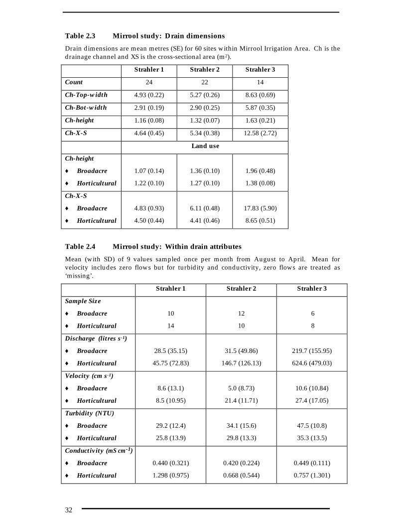
32
Table 2.3 Mirrool study: Drain dimensions
Drain dimensions are mean metres (SE) for 60 sites within Mirrool Irrigation Area. Ch is thedrainage channel and XS is the cross-sectional area (m2).
Strahler 1 Strahler 2 Strahler 3
Count 24 22 14
Ch-Top-width 4.93 (0.22) 5.27 (0.26) 8.63 (0.69)
Ch-Bot-width 2.91 (0.19) 2.90 (0.25) 5.87 (0.35)
Ch-height 1.16 (0.08) 1.32 (0.07) 1.63 (0.21)
Ch-X-S 4.64 (0.45) 5.34 (0.38) 12.58 (2.72)
Land use
Ch-height
♦ Broadacre
♦ Horticultural
1.07 (0.14)
1.22 (0.10)
1.36 (0.10)
1.27 (0.10)
1.96 (0.48)
1.38 (0.08)
Ch-X-S
♦ Broadacre
♦ Horticultural
4.83 (0.93)
4.50 (0.44)
6.11 (0.48)
4.41 (0.46)
17.83 (5.90)
8.65 (0.51)
Table 2.4 Mirrool study: Within drain attributes
Mean (with SD) of 9 values sampled once per month from August to April. Mean forvelocity includes zero flows but for turbidity and conductivity, zero flows are treated as‘missing’.
Strahler 1 Strahler 2 Strahler 3
Sample Size
♦ Broadacre
♦ Horticultural
10
14
12
10
6
8
Discharge (litres s-1)
♦ Broadacre
♦ Horticultural
28.5 (35.15)
45.75 (72.83)
31.5 (49.86)
146.7 (126.13)
219.7 (155.95)
624.6 (479.03)
Velocity (cm s-1)
♦ Broadacre
♦ Horticultural
8.6 (13.1)
8.5 (10.95)
5.0 (8.73)
21.4 (11.71)
10.6 (10.84)
27.4 (17.05)
Turbidity (NTU)
♦ Broadacre
♦ Horticultural
29.2 (12.4)
25.8 (13.9)
34.1 (15.6)
29.8 (13.3)
47.5 (10.8)
35.3 (13.5)
Conductivity (mS cm-1)
♦ Broadacre
♦ Horticultural
0.440 (0.321)
1.298 (0.975)
0.420 (0.224)
0.668 (0.544)
0.449 (0.111)
0.757 (1.301)

33
Table 2.5 Mirrool study: Chemical characteristics
Outcomes of two 1-way ANOVA (factor stream order, then factor land use), and a 2-wayANOVA (factors stream order x land use). NS means not significant.
StrahlerStream order Land use SO x Land Use
Conductivity NS p = 0.02
Hort >> BR
Land Use
Turbidity NS p = 0.01
BR >> Hort
Land Use
Suspended Sediment NS NS NS
Total Phosphorus p =<0.01
SO1 > SO2,SO3
p = 0.07
BR >> Hort
SO and LU
Filterable Phosphorus p=0.04
SO1 > SO2, SO3
p = 0.07
BR >> Hort
SO x LU
SO1 in BR >> rest
Ammonium Nitrogen NS NS NS
Oxidised Nitrogen NS p<0.001
Hort >> BR
SO x LU,
SO2 in Hort >> rest
Organic Nitrogen NS NS NS
Total Nitrogen NS p = 0.03
Hort >> BR
SO x LU
SO2 in Hort >>
Table 2.6 Mirrool study: Vegetation cover
Vegetation cover in a 5-metre transect in 60 drains classified by Strahler stream order anddominant land use. Cover values are mean % (with SD) of 9 values (unless ‘missing’) foreach site visited once per month from August to April. December data are given separately.
Strahler 1 Strahler 2 Strahler 3
Sample SizeSample Size
♦ Broadacre
♦ Horticultural
10
14
12
10
6
8
Drain vegetation (as% cover)
♦ Broadacre
♦ Horticultural38.0 (16.9)
59.8 (17.7)
39.7 (19.6)
30.7 (21.0)
23.7 (16.9)
26.0 (20.1)
Drain vegetation inDecember (% cover)
♦ Broadacre
♦ Horticultural41.2 (25.5)
71.4 (32.1)
49.8 (33.4)
23.8 (17.5)
37.4 (35.1)
37.5 (27.7)

34
Table 2.7 Basin application: Site details
Location and number of sites, and dominant land uses in their respective catchments at thetime of sampling (February 1995).
Irrigation Area and location Drain sites
Number and Date
Dominant Land uses
Coleambally NSW 11, on 6 February Broadacre
Lalalty NSW 8, on 20 February Pasture
Barmawm Vic 12, on 22 February Pasture
Shepparton Vic 9, on 21 February Horticulture
Tullakool NSW 10, on 23 February Pasture and Broadacre
Merungle Hill NSW 5, on 9 February Pasture and Broadacre
Murrami NSW 5, on 9 February Pasture and Broadacre
Table 2.8 Basin application: Channel dimensions
Number of drains in each land use x Stream Order combination, (number of irrigation areasin brackets). Top width and Bottom width were both measured but only Top width isshown.
SO1 SO2 SO3
Sample Size
♦ Pasture
♦ Broadacre
♦ Horticultural
8 (3)
7 (3)
3 (2)
7 (3)
7 (3)
4 (2)
6 (3)
3 (2)
2 (1)
Channel Top W (m)
♦ Pasture
♦ Broadacre
♦ Horticulture
5.81 (1.7)
4.57 (0.9)
3.0 (0.7)
5.67 (1.3)
6.9 (2.1)
2.88 (0.7)
8.20 (3.7)
9.0 (1.4)
3.75 (1.7)
Channel Bank height
♦ Pasture
♦ Broadacre
♦ Horticultural
1.26 (0.5)
0.91 (0.3)
1.37 (0.6)
1.50 (0.3)
1.5 (0.3)
0.83 (0.2)
2.0 (1.1)
1.7 (0.9)
1.0 (0)
Water X-S area (m2)
♦ Pasture
♦ Broadacre
♦ Horticultural
1.46 (2.1)
2.63 (3.8)
0.17 (0.2)
3.26 (4.6)
5.1 (3.1)
0.91 (0.4)
1.81 (1.5)
3.5 (1.6)
4.34 (2.6)

35
Table 2.9 Basin application: Vegetation
Mean (with SD) within-drain vegetation cover (as %) for 5-metre transects for 48 sites from 7irrigation areas in southern New South Wales and Victoria, recorded in February 1995.
SO1 SO2 SO3
Vegetation Cover (%)
♦ Pasture
♦ Broadacre
♦ Horticultural
54.3 (35.0)
64.9 (23.9)
13.6 (19.4)
24.4 (28.1)
48.6 (29.7)
17.8 (16.2)
33.7 (27.2)
61.0 (28.2)
76 (13.0)
Number of Species
♦ Pasture
♦ Broadacre
♦ Horticultural
4.1 (2.0)
4.6 (1.4)
2.2 (1.5)
2.8 (1.3)
4.3 (2.0)
2 (1.22)
2.8 (1.8)
6.0 (1.4)
5.5 (1.5)
Algal cover (%)
♦ Pasture
♦ Broadacre
♦ Horticultural
45.8 (44.5)
24.0 (30.2)
8.2 (11.5)
52.5 (35.3)
8.3 (9.6)
77.5 (22.8)
33.67 (37.0)
11.7 (6.2)
30.5 (29.5)

36
Table 2.10 Catchment analysis for Coleambally IA
Summary of characteristics for 12 sub-catchments in the Coleambally Irrigation Area, NSW.These were derived from a catchment map and have not been ground-truthed. Shape ismissing for the last catchment.
Area (ha) Perimeter(km)
Drainagelength (km)
Number ofescapes
Shape Density(km per
km2)
5123 58.2 30.5 2 pinnate 0.59
32,533 109.8 180 12 pinnate 0.55
5075 50.4 26.4 1 pinnate 0.52
2214 27.1 12.2 0 pinnate 0.55
15,315 68.7 78.6 8 pinnate 0.51
5077 40.4 19.7 2 pinnate 0.38
2243 26.5 16.2 3 pinnate 0.72
4543 40.8 17.1 3 pinnate 0.37
3367 50.2 23.3 0 pinnate 0.70
1007 42.8 9.9 0 pinnate 0.98
4192 45.9 30.3 4 pinnate 0.72
341 8.0 1.3 0 0.36

37
Figure 2.1 Pilot study: Stream orders in Hanwood sub-catchment
Diagram showing the drainage network in one of the two small catchments used in the PilotStudy. The numbers are Strahler stream orders. Note that despite the number of smalldrains around Hanwood village, and the complexity of the drainage network, the drainentering Main Drain J is only SO3. MDJ refers to Main Drain J

38
Figure 2.2 Mirrool study
The 60 sampling sites in the Mirrool IA covered three orders of drains, distributed bycatchment size (large v small) and dominant land use (broadacre v horticulture).

39
Stream Order and Vegetation Cover
0 1 2 3 4 5Stream Order
0
10
20
30
40
50
60
70
80
90
100
Veg
etat
ion
Cov
er (
%)
Figure 2.3 Pilot study: Vegetation cover
Box and whisker plot showing the distribution of values for vegetation cover in 36 drains inHanwood and South Griffith catchments, in the Mirrool Irrigation Area, in winter 1994, bystream order. Median values are horizontal line within each box, the box encloses 75% ofthe data values, and outliers are indicated by circles and crosses.
Cover: Annuals and Perennials
0 1 2 3 4 5Stream Order
0
10
20
30
40
Veg
etat
ion
Cov
er (
%)
AnnualsPerennials
Figure 2.4 Pilot study: Vegetation cover based on life history
Mean (with SE) cover of Annuals and Perennials in 36 sites in South Griffith and Hanwoodcatchments within the Mirrool Irrigation Area, in winter 1994.

40
Drain Dimensions
0 1 2 3 4Stream Order
0
10
20
30
40
50
Cro
ss-s
ectio
nal a
rea
(m2)
BroadacreHorticultural
Dominant Land Use
Figure 2.5 Mirrool study: Drain dimensions
Mean cross-sectional area of drains (with SE) in Mirrool Irrigation Area, showing how thisincreases with increasing stream order, but is dependent on land use.
Figure 2.6 Mirrool study: Incidence of zero flows
Incidence of zero flows in 28 drains from broadacre catchments and in 32 drains inhorticulture-dominated catchments, in the Mirrool IA from August 1994 to April 1995. Thesmall samples sizes for each stream order x land use combination means that incidencevalues (as %) appear to give anomalous results.

41
Chapter 3Chapter 3
The Trunks and The Trunks and Tribs StudyTribs Study: Lateral Drains: Lateral Drains
3.13.1 Targeting the hot-spotsTargeting the hot-spotsAn essential part of management is understanding the dimensions of the problem.Where the problem is nutrients, and the objective is to reduce the export of nutrientsin drainage water, the dimensions include the choice of solution (here, the use ofmacrophytes), and its location. In this sense, location means knowing where andwhen to implement nutrient reduction.
Within an irrigation area, there are three types of location: at source (ie on-farm), atexit (in main exit drain) or in-between (irrigation drainage network). Exit drains arethe monitoring point for environmental compliance and licensing. Monitoring sitesare matched to a gauging station so have the longest data sets within an irrigationarea. These exit drains are where the existence of a nutrient problem is typicallydiagnosed. Exit drains, however, are relatively high stream order sites (eg SO4 sites)and are neither optimum nor suitable sites for improving water quality. Their valueas macrophyte habitat (considered in Chapter 8) is not high, and they are anintegration of upstream water. Treating water at this point ignores differences insources and means that both acceptable and poor quality are being targeted, whichis potentially inefficient.
The alternative is to treat drainage water within the irrigation network. Eventhough nutrient concentrations and loads are not extensively documented, they canbe expected to vary throughout the irrigation area. Reasons for making such anassumption are the enormous diversity of crops grown. This, coupled with theindividual styles of farming, whether cultivating or in the use and application offertilisers, means nutrient concentrations and loads will vary widely not justthrough an irrigation area, but also through an irrigation season. The challenge is toidentify these nutrient hot-spots, without actually monitoring every drain.
The approach suggested here is an extension of the catchment concept. It treats anirrigation area as a series of sub-catchments and uses a stratified approach to samplethese, using dominant crop type and flow type (base or flood) as factors.
Because land use affects water quality, catchments with different land uses havedifferent nutrient yields (eg Young et al. 1996). Very few yields have been estimatedfor irrigation crops in Australia, although the significance of crop type for waterquality has been recognised. Harrison (1994) used a scatter plot used to show thathorticultural drainage was typically high in nitrogen and low in phosphorus,whereas pasture drainage was usually low in nitrogen but high in phosphorus. Thedata set was drawn from a number of irrigation areas and was not time specific.
The effect of land use on water quality is not constant but can change with rainfall.High run-off entrains other sources of nutrients hence the relationship between landuse and water quality appears to vary with discharge. It was for these reasons, thatthe Basin-wide modelling of nutrient export (GHD 1992) was careful to recognisedifferent hydrological conditions, using ‘average’, ‘dry’ and ‘wet’ years. For thesereasons, this study distinguishes between low-flow and high flow conditions.

42
ObjectivesObjectivesThe objective was to determine if land use, a catchment characteristic, could beuseful for locating nutrient hot-spots within an irrigation area. This was done bydocumenting nutrient concentrations and loads, for a number of drains. hot-spotswere then identified by reference to individual drains and results compared withdrains aggregated by land use. This addressed the question of the location of hot-spots but not their timing.
The focus was on low-flow conditions during the irrigation season and into autumn.This was done deliberately as the effect of macrophytes on water quality is likely tobe greater under low flows than during periods of high discharge. Conditions otherthan low-flow are covered separately (Chapter 4).
Specific objectives were:
♦ To document seasonal variations in nutrient concentrations and loads underlow-flow conditions in lateral drains
♦ To determine if there are distinctive water qualities associated with specific landuses, and define what these are
♦ To determine whether land use is effective in identifying specific drains orcatchments for nutrient reduction.
Because it is based on a large exit drain (Main Drain J) and on several tributarydrains, this study became known as the Trunks and Tribs study.
3.23.2 MethodsMethods
Study areaStudy area The study area was the eastern part of the Mirrool Irrigation Area (Figure 3.1). Itextended north and east of Griffith, and included the villages outside Griffith suchas Yenda, Beelbangera, Bilbul and Yoogali. Between Yenda and Yoogali, there are12-15 drains which are parallel, evenly-spaced and of similar length, thus thedrainage network here is noticeably pinnate-rectangular (Gordon et al. 1992, p102).Several small almost rectangular catchments discharge directly into Main Drain J.These are similar in size and shape, but not necessarily in land use. The originalintention was to use these drains and sub-catchments as a series of ‘replicates’,without the confounding effect of catchment size. However, as this study becamecombined with the study on Main Drain J (Chapter 5), other drains and sub-catchments of varying size were included and this aspect of the design becamesubmerged.
Catchment area and main land uses in each sub-catchment were measured from acolour photomosaic of the study area taken in January 1995 using an image analysispackage DT-Scan. Land use types were ground-truthed in December 1996, andagain in 1998.
Site set upSite set up A site was located in each of the lateral drains discharging into Main Drain Jbetween Yenda and Old Willbriggie Road, south of Griffith (Figure 3.1). This gave atotal of 24 sites, numbered 1-24, in sequence down Main Drain J, and are named forthe road adjacent (eg Table 3.1).

43
Sampling points were at least 5-10 metres from Main Drain J and within the lateraldrain. They were thus upstream of the point where the lateral drain falls, by 1 metreor more, into Main Drain J. These drops are only evident during lowest flowconditions in low rainfall winters. This was considered to be the optimum positionto avoid backflow effects from Main Drain J whilst being representative of the drainitself and its upstream catchment.
Three tributary drains were overlooked in setting up the sampling program. Onewas next to Clark Lane, north-east of Yoogali, and one was an urban input fromYoogali; both were small and were never seen flowing. The third, at KurrajongAvenue, carried a small flow of urban, industrial and horticultural drainage. Thisdrain was not included by Bowmer et al. (1992) in their turbidity budget.
Field study and samplingField study and sampling Sites were sampled monthly (9 times) from October 1994 to June 1995, inclusive. All24 sites were sampled in a single day, and all sampling started at the most upstreamsite (Site 1) and finished at the site furtherest downstream (Site 24) As this studywas for low flow conditions, no sampling was done during or immediately afterrainfall and if necessary, sampling was postponed for a few days.
Weather in 1994-95 irrigation season was initially quite dry. Total rainfall for theyear was 215.3 mm compared with the long-term mean of 398 mm (Table 1.1 above).In contrast, rainfall during the first six months of 1995 was well above average.Despite this, there was a prolonged dry spell in late summer, with no rain between 6February and 5 April 1995
The time between sampling and preceding rainfall was: 5 days (3 mm on 8th) inOctober; 5 days (2 mm on 19th) in November; 8 days (14.4 mm on 8th) in December;5 days (19.8 mm on 20th) in January; 16 days (11.2 mm on 5th) in February; 38 daysin March (no rain since 5th February); 59 days in April (no rain since 5th February); 7days in May (1 mm on 4th and 28.6 mm on 2nd); and 3 days in June (0.4 mm on 3rd
June, and 1 mm on 26th May).
On each visit, and at each site, discharge was measured and a 500 mL water samplewas collected from just below the water surface in mid-stream. Water samples wereanalysed for electrical conductivity (EC), turbidity, suspended solids (SS), totalphosphorus (TP), oxidised nitrogen species (NOx), organic nitrogen as TotalKjeldahl nitrogen (TKN) and dissolved ammonium nitrogen (NH4). Total nitrogen(TN) was estimated as the sum of NOx and TKN. Samples were stored andtransported back to the laboratory following standard procedures for this laboratory(Appendix 4). Abbreviations for nutrients are used henceforward.
Data presentation and analysisData presentation and analysis Land use types Three land use types, based on combinations of twodominant land use in the sub-catchment. Horticulture (H) included grapes, citrus,stone fruits and other horticultural crops, and broadacre (BR) included rice andpasture. The three combinations were H-50, where 50% or more of catchment washorticulture, BR-50, where more than 50% of catchment was broadacre, and BR-100where the entire catchment was broadacre.
Among the 24 sub-catchments there were five H-50, ten BR-50 and the remaining 8were BR-100 (Table 3.1). One catchment was not assigned a dominant land use (Site

44
3) because it was used primarily as a water supply channel, passing water from themain supply system to Main Drain J (Chapter 1.4).
The relationship between land use and water quality can be complicated by otherinputs such as roadside drains discharging directly into Main Drain J after rain, tiledrain pumps (only in horticultural areas), supply water being routed through somedrains (Sites 3 and 20), and urbanisation. For example, there were 21 tile drainpumps into Main Drain J of which 19 were between Sites T and Y, and 2 betweenSites Y and B (Figure 3.1 for location of Sites T, Y and B on Main Drain J). Urbanareas were small, and affected only three catchments (Sites 2, 11 and 20).
Trends Temporal (monthly readings) and spatial (24 tributary drains) trendswere explored graphically and by using summary statistics, the mean and median.The mean was generally used when data set was small, for example for monthlytrends (max n = 9 months), and the median used for summarising trends acrossdrains (max n = 24 drains).
Water quality of drains with similar land use was explored by stratifying nutrientreadings according to land use (BR-100, BR-50 and H-50). Box-and-whisker plotswere used to graphically show the distribution of values around the median(SYSTAT 6.0). Statistical summaries tabulated for each drain use mean and standarderror of the mean (SE) or standard deviation. The graphing module gave a slightdistortion in presentation of mean values so plots are indicative only.
Water quality assessment Where appropriate, individual results ofnutrient concentrations were ranked Medium or High following the criteriasuggested by Harrison (1994), set out below. Nutrient loads were also ranked, butusing a relative rather than an absolute system. The top five were considered high.
Criteria TP (mg L-1) TN (mg L-1) NOx (mg L-1)
Low <0.1 <1 < 0.5
Medium 0.1 - 0.5 1 - 5 0.5 - 2.5
High > 0.5 > 5 > 2.5
Loads Loads were calculated for the major water quality parameters,namely SS, TP, TN, TKN and NOx, as the product of concentration andinstantaneous discharge. Loads are presented as kg d-1. Total load for the studyperiod is the sum of the load for each of nine months. This makes a conservativeassumption that low-flow conditions when sampling lasted throughout each month.
Land use signature Correlation analysis was used to identify relationshipsbetween pairs of water quality parameters; Bartlett’s chi-square test statistic wasused to determine the significance of the correlation between pairs of parameters.Regression analysis was used to explore the relationship between turbidity and SS,and 95% confidence limits of the intercept are reported.
3.33.3 ResultsResults Discharge Even under low flow conditions, discharge in the 24 lateral drainswas highly variable, as shown by mean discharge and standard deviation (Figure

45
3.2). The source of this variability was largely due to differences in catchment size.Catchment area and median flow were highly correlated (r = 0.98).
Although in general, smaller catchments had generally lower discharges and largercatchments had higher discharge, this was not always true. For example, the lowestmedian flows for an individual tributary (Table 3.2) was <1 ML d-1 for Site 15(Moseley Road), which was not the smallest sub-catchment. The converse, however,appeared to hold. The highest median flow was 590 ML d-1 at Site 20 (McCormack’sRoad), which was the biggest sub-catchment, and the three drains with medianflows greater than 100 ML d-1 (Sites 20, 2 and 24) were the three largest catchments(Table 3.1).
The highest instantaneous discharge (under low flow conditions) in a tributary drainwas 1200 litres s-1, at Site 20 in January 1995. Although effort was made to minimisethe effect of rainfall, this high reading may have been a consequence of nearly 20mm rain on 20th January, five days earlier (Chapter 4). The lowest instantaneousdischarge was zero. On nearly all occasions during the irrigation season whendischarge was recorded as zero, the drain was not dry but water was ponded andwater samples were collected.
Zero flows From April onwards, irrigation season began to close. Irrigationsupply typically ceases by the end of May. Thus in June 1995, when monitoringceased, only five drains were still flowing (Sites 2, 7, 20, 22 and 24). Once theirrigation season ends, the water in drains is not irrigation drainage but comes fromtile drain sumps, escape and supply water, and some groundwater interception(Chapter 1 4), as well as urban activities and rainfall run-off. Zero-flows inbroadacre drains in December (Figure 3.2 lower) may be attributed to the practice oflocking up rice. The reason some horticultural drains were not flowing in Octoberwas probably that grapes were not being irrigated at that time (Warren Muirhead,pers. comm. 1998).
The total frequency of zero flows (number of times an individual drain was recordedas having no flowing water, max value = 9) was not strongly linked to land use(Table 3.3) although BR catchments tended to be dry more often. Comparisonbetween the three land uses (Figure 3.2) shows the incidence of zero flows increasedin all land uses from April onwards, but was distinctly higher in broadacrecatchments. Although this trend is consistent with citrus and vines having a longerirrigation season than rice, land use may not be the sole explanation for thesedifferences in discharge. For example, tile drains may be activated by heavy rainfalland may pump out groundwater. This could have occurred in May and June 1995as this was a time of above-average rainfall (Table 1.1 below). Some drains, notablySite 3 at McKissack Road, appear to have been used periodically to deliver supplywater from the Main Canal supply system through to Mirrool Creek. Consequently,these drains will have higher discharge than expected for a given catchment size,and will remain flowing beyond the main irrigation season.
Concentrations, seasonal trends Water quality in the 24 tributary drainschanged through the growing season (Figure 3.3) but the seven water qualityparameters did not change synchronously. Moreover the distribution of values, asrepresented by the central 50% (the length of the box in the box-and-whisker plots)and the number of extreme values (Figure 3.3) showed that water quality washeterogeneous across the drains for nearly all the parameters measured.
The main points in the seasonal trends were:

46
♦ EC was generally low through the irrigation season until April, with medianvalues of 168-335 and mean values of 333-610 µS cm-1. After April, conductivitygenerally increased. High values, that is conductivity readings of 1000-4000 µScm-1, occurred throughout the study period.
♦ Turbidity showed a marked seasonal increase then decrease. This was a 3-4 foldincrease from November to February: median values rose from 17 to 67, meanfrom 22 to 74 NTU.
♦ SS showed the same trends as turbidity, with a pronounced peak in February-March. The high readings in January-March (> 200 mg L-1) were more typical offlood conditions.
♦ TP was consistently low (median = 0.09-0.17 mg L-1, mean = 0.06-0.11 mg L-1)throughout the study period. Values greater than 0.5 mg L-1 (which would beranked as High) were unusual. However, some exceptionally high TPconcentrations did occur, such as 1.86 mg L-1 at Site 1 in October (not shown inFigure 3.3). Other instances of High TP were > 1 mg L-1 at Sites 5 and 24 inOctober, and Sites 10 and 15 in March. These occasional very high values areassumed to be the result of irrigation drainage shortly after fertiliser application.
♦ TN concentrations were generally in the Medium range with median values of0.58 to 1.92 mg L-1 and mean values of 1.07 to 4.39 mg L-1. High readings, inexcess of 5 mg L-1 were not uncommon, occurring in every month of the study.Exceptionally high TN concentrations, greater than 10 mg L-1, also occurred.
• Only two forms of nitrogen are reported here, organic and oxidised.Ammoniacal-nitrogen was generally below detection limits and when present didnot contribute much.
• TKN was fairly constant with no seasonal patterns. Median and mean valueswere similar, with median ranging from 0.48 to 1.27 mg L-1 and mean from 0.61 to1.61 mg L-1. There were few instances of High and extremely High TKNconcentrations. Although NOx was consistently lower than TKN (median = 0.01 -0.19 mg L-1 and mean = 0.44 - 1.49 mg L-1), there was a persistent suite of Highdata throughout the year. NOx increased sharply at the end of the study period,with median and mean values of 1.29 and 3.67 mg L-1. Low values were due inpart to a number of samples with non-detectable concentrations.
Water quality in individual drains Median and mean values for the seven waterquality parameters (Table 3.4) confirm the heterogeneity of the 24 irrigation drains.Points specific to individual parameters are as follows:
♦ EC and NOx (and to a lesser extent TN) showed the greatest range in medianvalues. For EC, median values ranged from less than 120 (Sites 3 and 16) tomore than 1500 µS cm-1 (Sites 15 and 23). For NOx, median values ranged frombeing generally undetectable (at 12 sites) to more than 2.0 mg L-1 at four sites(Sites 2, 13, 15 and 23).
♦ TP and turbidity were the only two parameters which were generally low, andhad virtually no instances of being High. Only four drains had median TPconcentrations that were Medium (Sites 1, 10, 19, 23); another set of four drainshad mean TP that was High occasionally (Sites 1, 5, 15 and 24). Only four hadmedian turbidity greater than 40 NTU (Sites 7, 19, 20 and 21). Drains with low-flow TP close to supply water (Appendix E) were Sites 2, 3, 4, 7, 11, 13 and 18;

47
and drains with median turbidity close to or less than supply were Sites 7, 8, 9.19, 20, 21.
♦ Seven drains did not have elevated nutrients or poor water quality (Sites 3, 4, 12,14, 16, 18 and 22). It was not clear if this was due to conservative land or watermanagement practices. At least one of these (Site 3 at McKissack Road) receivedescape water so its nutrient concentrations and loads were diluted.
Water quality by land use Catchment land use was important in determining thetemporal variations in water quality, as shown by the monthly data during theirrigation season (Figure 3.4). The differences between the three land use types werereasonably consistent, as follows:
♦ EC in drainage water from BR-100 catchments was consistently lower andshowed much less seasonal variation. Drainage from BR-50 and H-50catchments had similar mean conductivity (there is a slight distortion in theplotting package used which makes BR-50 look intermediate) but H-50 wasclearly highest in June.
♦ All three land uses showed similar temporal trend in SS with a marked peak inFebruary. SS was generally lower at sites draining BR-100 catchments, butsimilar for BR-50 and H-50 catchments.
♦ All three land uses had a similar seasonal TP pattern, which was similar to SS,but the seasonal peak was much more subdued than SS. Differences betweenthe land uses were neither consistent nor clear (Figure 3.4).
• The link between land use and water quality was particularly clear with TN.Drainage from BR-100 catchments consistently had lowest mean TNconcentrations and H-50 the highest (except in April) with BR-50 catchmentsbeing intermediate. All three land uses followed a similar trend with a generaldecrease in mean concentration from late summer to autumn, followed by anincrease. The autumn increase was most marked in H-50 catchments (Figure 3.4).
Water quality land use signature Correlation analysis of concentration dataconfirmed the trends described above, namely that drainage from catchmentsdominated by a particular land use had a specific suite of characteristics (Table 3.5).The following points are relevant:
♦ Turbidity and SS were highly correlated, and each land use had a Pearsoncorrelation coefficient greater than 0.84 (not shown). Regression analysis of SSon turbidity was significant. The resulting regression coefficients were similar(see below) and the 95% confidence limits (not given) overlapped, suggesting asimilar SS-turbidity relationship for each land use. :
For BR-100, Turbidity = 13.49 + 0.46 SS (in mg L-1)
For BR-50, Turbidity = 11.28 + 0.41 SS (in mg L-1)
For H-50, Turbidity = 4.43 + 0.46 SS (in mg L-1)
The distinctive water quality characteristics of each land use type are (Table 3.5):
♦ In BR-100 catchments, TP correlates positively with TN, TKN with TN, NOxwith TN, and TP with TKN.
♦ In BR-50 catchments, TKN correlates positively with TP, also NOx with TN, andTurbidity with TP, SS with TP, NOx with EC and TN with EC.

48
♦ In H-50 catchments, TP correlates with SS, NOx correlates positively with TN,EC correlates with NOx, and EC with TN.
Thus two land uses (BR-100 and H-50) have drainage water quality that is quitedistinctive. Not surprisingly, given its intermediate nature, BR-50 sharescharacteristics with both (Table 3.5).
Loads from individual drains As expected, loads exported from 24 drains (Table3.6) showed considerable range. In absolute terms, SS were the largest loads,ranging from 1.7 to as much as 14,643 kg d-1. In contrast, highest load of individualnutrients delivered into Main Drain J under low flow conditions was 15.0 kg d-1 forTP, 126.5 for TN, 74.8 for TKN and 51.5 for NOx (Table 3.6).
Drains with the highest nutrient loads under low-flow conditions (Table 3.7)consistently included Sites 20, 2 and 24. These three drains also had the highestdischarge, and were the only ones with an average low-flow discharge exceeding100 L s-1 (Figure 3.2). Other drains contributing large nutrient loads into Main DrainJ were Sites 1, 8 and 13, but this second group did not necessarily have highestdischarge (Figure 3.2). Comparison of median discharge with mean concentrations(Table 3.4) shows that discharge was a greater influence on large export loads thanconcentration. Drains with the lowest nutrient loads were consistently Sites 3, 18and 23; all these had low but not the lowest discharge (Figure 3.2).
Loads for land use Highest mean loads of SS and TP came from BR-50 catchments,with a mean of 984.9 kg SS d-1 per drain and 1.11 kg TP d-1 per drain, and alsohighest load of TKN, with 12.7 kg d-1. The highest TN and NOX from H-50catchments, with mean of 26.0 kg TN d-1 and 18.8 kg NOx d-1 per drain. However,there is considerable range of values for all land uses (Figure 3.5).
3.43.4 DiscussionDiscussion
Identifying low-flow hot-spotsIdentifying low-flow hot-spots As anticipated, the Trunks and Tribs study of 24 lateral drain sites flowing into MainDrain J showed that the quality of drainage water in the Mirrool Irrigation Area wasnot constant through time nor uniform between drains. Thus the identity of anutrient hot-spots depends on whether it is load or concentration that is the issue.
If the issue is low-flow loads, then catchments contributing relatively more tonutrient export load can be identified by:
♦ Catchment size, disregarding type of land use The catchments with thehighest low-flow discharge and loads (Table 3.1) were the three largest, Sites 20,2 and 24.
However, if annual loads are the issue, then high discharge events (Chapter 4)should be monitored, and appropriate action diagnosed. If it is low-flow loads thatare the issue, then better water management practices should be considered.
If concentrations are the issue, then catchments where nutrient concentrations arehighest can be identified by:
♦ Land use Mean values or a relationship is needed to target likely sites. Forexample, mean values for H-50 catchments showed the drains most likely tohave high EC and high NOx or TN. Thus selecting H-50 drains would targetSites 2, 13, 16, 22, 23 and 24.

49
♦ Individual drains Monitoring all drains shows that the drains with highestmean EC and NOx were (Table 3.4) 2, 5, 11, 13. 15, 17, 20, 23 and 24 and Sites 2,13, 15, 17, 20, 23 and 24, respectively.
However, if absolute concentrations are needed, ie places where concentrationsexceed an absolute value and how often, then conventional monitoring may beneeded. Thus the aggregated criteria, land use, was effective in identifying thedrains with high NOx. However, as the mean values for H-50 do not include highvalues of TP or turbidity, using H-50 would be an inappropriate way to target drainswhere TP and high turbidity were a problem.
With respect to loads:
♦ By land use Using land use to identify major contributors of nutrientloads is not effective because of the influence of discharge. Thus, using BR-100,because it has the highest mean TP concentration (Table 3.5), as an indicator ofwhich drains are contributing highest TP loads selects Sites 1, 4, 5, 6, 7, 8, and 9of which only one (Site 8) is possibly appropriate.
♦ Individual drains Calculating mean loads (Table 3.6) shows that highestexporters of SS, TP, TN and NOx were Sites 20, 2 and 24 followed by Sites 8, 13and 19 (Table 3.7).
♦ By discharge Discharge can be effective in selecting those sites with highestloads. The three sites with the highest discharge (Sites 2, 20 and 24 with landuses H-50, BR-50 and H-50) are all high exporters of SS and nutrients (Table 3.6).Discharge may be less effective a discriminator where sites are similar. Thesethree sites have median discharges which are at least 50% higher than others.
Discharge therefore remains the most effective criteria for identifying sources of highnutrient loads.
Identifying the timing of hot-spots can be done either by monitoring, to establish theyear-round pattern and occurrence of seasonal peaks, or by inference fromknowledge of fertiliser usage and irrigation practices, provided these are confidentlyknown to be the main source of nutrients. The identification of prolonged high SSconcentrations and occasional transient TP peaks suggests seasonal patterns need tobe confirmed, rather than assumed.
Monitoring through this study (Figure 3.3.) showed the peaks were:
♦ Individual drains SS was highest in February-March, TP in January and March,TN and NOx in June, and TKN in November-February.
The value of monitoring for identifying times of highest nutrient concentration canbe improved if land use is included (Figure 3.4).
♦ Land use SS in February-March, TP in December-January-February, TN inOctober-November and May-June especially in H-50 catchments.
Findings and conclusionsFindings and conclusions The Trunks and Tribs study documented spatial and temporal patterns in nutrientconcentrations and loads under low-flow conditions for 24 drains in the MirroolIrrigation Area, over a nine-month period. These data were used to develop criteriafor identifying where and when nutrient concentrations were highest.
For identifying Where, the following was established:

50
♦ The dominant land uses in irrigation areas have distinctive water qualitysignatures, in terms of mean nutrient concentrations and composition. Whenthese signatures are distinct, then intermediate signatures and valuescorresponding to mixes of land use, can also be identified.
♦ Land use is an effective means of pinpointing drains and catchments within anirrigation area where nutrient concentrations are high, providing that the linkbetween land use and water quality (nutrient concentration) has beenestablished.
♦ Even under low-flow conditions, discharge is an effective means of identifyingthe drains and catchments which are major exporters of nutrient loads. Ifdischarge is not available, catchment size is a feasible alternative, providing landuse remains unchanged.
♦ Discharge is not an appropriate means of identifying the lowest exporters.
For identifying When, the following was established
♦ Monitoring for a year is essential in order to establish the basic seasonal patternand identify nutrient peaks.
Macrophyte locationMacrophyte locationThe spatial and temporal patterns of nutrients documented in the 1994-1995irrigation season are thought to be reasonably representative of low-flow conditionsin the Mirrool Irrigation Area. The nutrient hot-spots identified by this 9-monthmonitoring, under low-flow conditions in the eastern part of the Mirrool IA, aresummarised below. The strategic use of macrophytes to target nutrients at thesetimes and places means growing in the conditions represented by these conditions,interpreted below.
Horticulture-dominated sub-catchments These had the highest TN and NOxconcentrations, with pulses occurring in spring (October-November) and autumn(May-June). The growing conditions encapsulated by these two time frames arequite different. In October and November, being times of high drainage, flow isrelatively deep, fast-flowing and turbid but temperatures and daylength areincreasing. In autumn, flows are very low, water is shallow and becoming clearerwith low turbidity but conductivity can be quite high.
High TP sites Drains where TP was ranked High, following the rankingsystem of Harrison (1994), were Sites 1, 5, and 24 in October, and Sites 10 and 14 inMarch. Drains with persistent high TP concentrations, as indicated by their medianvalues (Table 3.4) were Sites 1, 6, 10, 19 and 23. Together these cover all three typesof land use (Table 3.4); they drain catchments of medium size (Table 3.1) butwithout large flows (Figure 3.2). Thus these represent spring-summer growingconditions, in predominantly fresh but turbid water, under a range of flow regimes(velocity and depths).
These two hot-spots highlight the range of growing conditions for macrophytes inirrigation drains. Such a diverse habitat conditions will require more than onespecies.

51
ReferencesReferencesBowmer, K.H., Bales, M. and Roberts, J. (1992). The effect of aquatic plants on water quality in
irrigation drains: a feasibility study for the Murray-Darling Basin Commission. CSIRODivision of Water Resources, Griffith. Consultancy Report 92/17. June 1992.
Gordon, N.D., McMahon, T.A. and Finlayson, B.L. (1992). Stream hydrology; an introductionfor ecologists. John Wiley & Sons, Chichester.
GHD (1992). An investigation of nutrient pollution in the Murray-Darling River system. Reportprepared by Gutteridge, Haskins and Davey, for the Murray-Darling BasinCommission.
Harrison, J. (1994). Review of nutrients in irrigation drainage in the Murray-Darling Basin.CSIRO Division of Water Resources. Seeking Solutions. Water Resources Series:No 11.
Young, W.J., Marston, F.M. and Davis, J.R. (1996). Nutrient exports and land use inAustralian catchments. J. Environmental Management 47:165-183.

52
Table 3.1 Sampling sites
Summary of site and catchment characteristics giving name and number, catchment areaand land uses (as %).
Key: MDJ means Main Drain J; Area refers to catchment area, and % of catchment that isBroadacre (pasture, rice, row crops and winter cereals), Horticulture (citrus, grape vines,stone fruits) or Urban (village). Catchments are grouped by land use as follows: BR-100 isall Broadacre, BR-50 is >50%and <100% Broadacre, H-50 is = >50% horticulture. Sites T, Yand B on Main Drain J, and reported on in Chapter 5. n.m. means not measured.
Area (ha) % Broad % Hort % Urban Type
T TOP of MDJ
1 Cotterill Road
2 Yenda Drain
3 McKissack Road
4 Marchington Road
5 EK Jones Road
6 Condon Road
7 Chauncey Road
8 Bilbul Road
9 de Bortoli Road
10 Lawrence Road
11 Kearey Road
12 Prior Road
13 McDonald Road
14 Fallon Road
15 Moseley Road
16 Evans Road
17 Savage Road
18 Poletta Road
19 Ross Road
20 McCormack Road
Y near Yoogali gauge, MDJ
21 Morely Road
22 Centofanti Road
23 Ceccato Road
24 Watkins Avenue
B ‘Bottom’, MDJ
213
247
1613
n.m.
612
310
321
631
673
299
279
218
252
208
238
327
264
247
261
263
8038
13,591
252
282
56
808
15,339
100
100
0
0
100
100
100
100
100
100
80
79
90
40
90
60
50
70
70
85
77
60
40
0
30
0
0
91
0
0
0
0
0
0
0
20
20
10
60
10
40
50
30
30
15
23
40
60
100
70
0
0
9
0
0
0
0
0
0
0
0
1
0
0
0
0
0
0
0
0
<1
0
0
0
0
BR-100
BR-100
H-50
n.a.
BR-100
BR-100
BR-100
BR-100
BR-100
BR-100
BR-50
BR-50
BR-50
H-50
BR-50
BR-50
H-50
BR-50
BR-50
BR-50
BR-50
BR-50
H-50
H-50
H-50
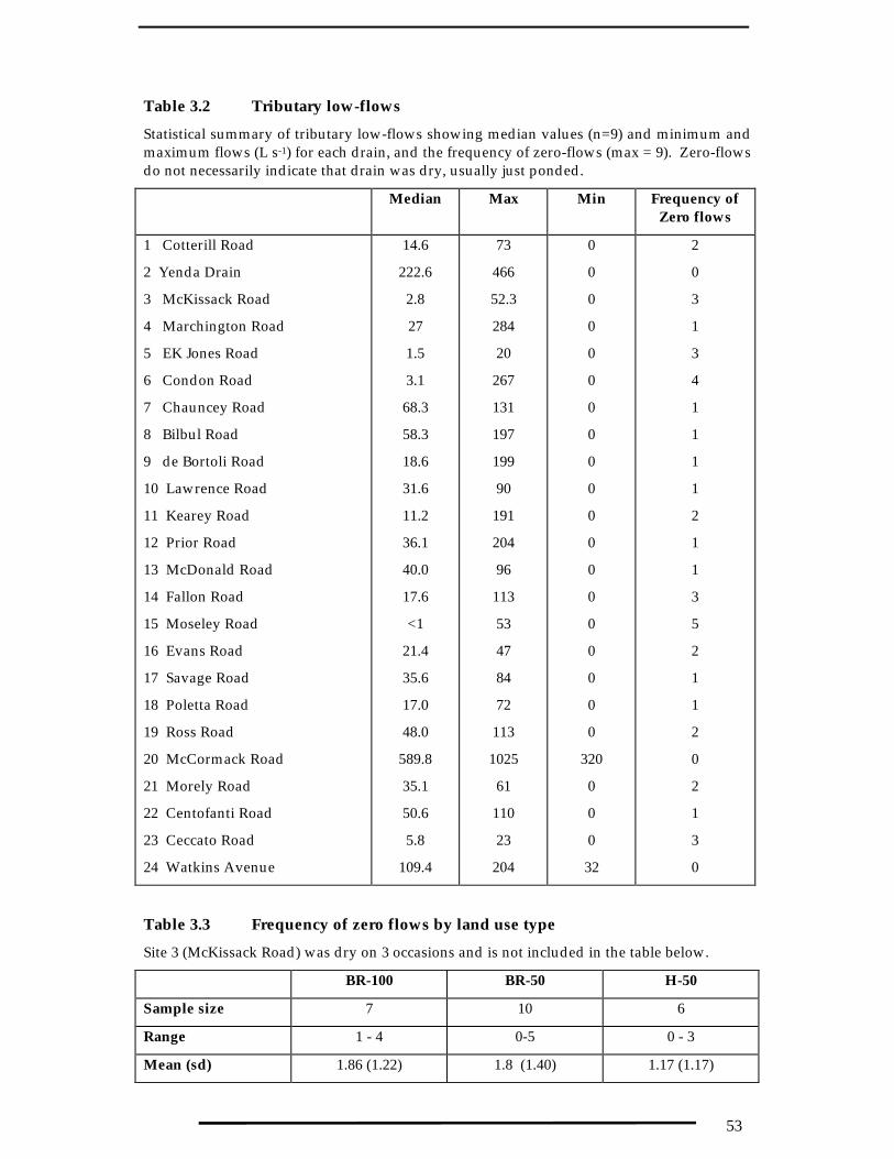
53
Table 3.2 Tributary low-flows
Statistical summary of tributary low-flows showing median values (n=9) and minimum andmaximum flows (L s-1) for each drain, and the frequency of zero-flows (max = 9). Zero-flowsdo not necessarily indicate that drain was dry, usually just ponded.
Median Max Min Frequency ofZero flows
1 Cotterill Road
2 Yenda Drain
3 McKissack Road
4 Marchington Road
5 EK Jones Road
6 Condon Road
7 Chauncey Road
8 Bilbul Road
9 de Bortoli Road
10 Lawrence Road
11 Kearey Road
12 Prior Road
13 McDonald Road
14 Fallon Road
15 Moseley Road
16 Evans Road
17 Savage Road
18 Poletta Road
19 Ross Road
20 McCormack Road
21 Morely Road
22 Centofanti Road
23 Ceccato Road
24 Watkins Avenue
14.6
222.6
2.8
27
1.5
3.1
68.3
58.3
18.6
31.6
11.2
36.1
40.0
17.6
<1
21.4
35.6
17.0
48.0
589.8
35.1
50.6
5.8
109.4
73
466
52.3
284
20
267
131
197
199
90
191
204
96
113
53
47
84
72
113
1025
61
110
23
204
0
0
0
0
0
0
0
0
0
0
0
0
0
0
0
0
0
0
0
320
0
0
0
32
2
0
3
1
3
4
1
1
1
1
2
1
1
3
5
2
1
1
2
0
2
1
3
0
Table 3.3 Frequency of zero flows by land use type
Site 3 (McKissack Road) was dry on 3 occasions and is not included in the table below.
BR-100 BR-50 H-50
Sample size 7 10 6
Range 1 - 4 0-5 0 - 3
Mean (sd) 1.86 (1.22) 1.8 (1.40) 1.17 (1.17)
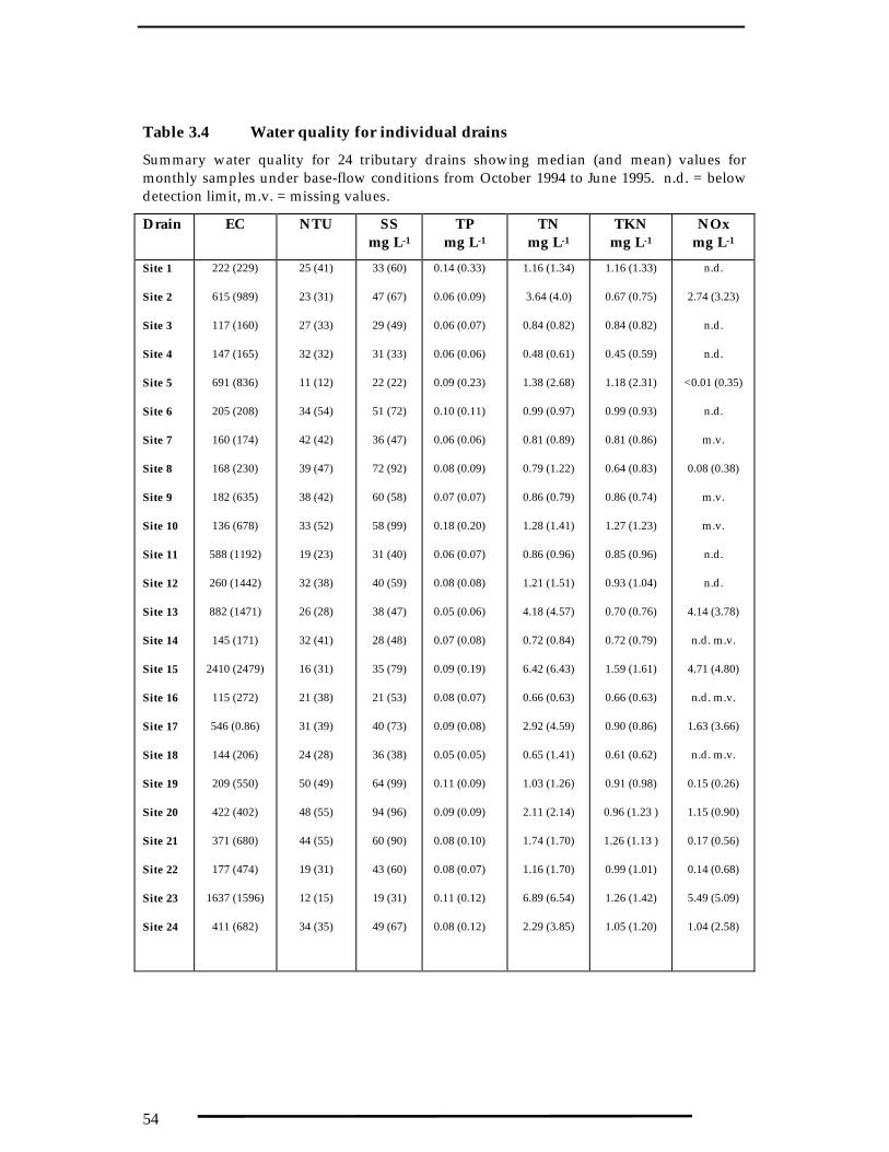
54
Table 3.4 Water quality for individual drains
Summary water quality for 24 tributary drains showing median (and mean) values formonthly samples under base-flow conditions from October 1994 to June 1995. n.d. = belowdetection limit, m.v. = missing values.
Drain EC NTU SSmg L-1
TPmg L-1
TNmg L-1
TKNmg L-1
NOxmg L-1
Site 1
Site 2
Site 3
Site 4
Site 5
Site 6
Site 7
Site 8
Site 9
Site 10
Site 11
Site 12
Site 13
Site 14
Site 15
Site 16
Site 17
Site 18
Site 19
Site 20
Site 21
Site 22
Site 23
Site 24
222 (229)
615 (989)
117 (160)
147 (165)
691 (836)
205 (208)
160 (174)
168 (230)
182 (635)
136 (678)
588 (1192)
260 (1442)
882 (1471)
145 (171)
2410 (2479)
115 (272)
546 (0.86)
144 (206)
209 (550)
422 (402)
371 (680)
177 (474)
1637 (1596)
411 (682)
25 (41)
23 (31)
27 (33)
32 (32)
11 (12)
34 (54)
42 (42)
39 (47)
38 (42)
33 (52)
19 (23)
32 (38)
26 (28)
32 (41)
16 (31)
21 (38)
31 (39)
24 (28)
50 (49)
48 (55)
44 (55)
19 (31)
12 (15)
34 (35)
33 (60)
47 (67)
29 (49)
31 (33)
22 (22)
51 (72)
36 (47)
72 (92)
60 (58)
58 (99)
31 (40)
40 (59)
38 (47)
28 (48)
35 (79)
21 (53)
40 (73)
36 (38)
64 (99)
94 (96)
60 (90)
43 (60)
19 (31)
49 (67)
0.14 (0.33)
0.06 (0.09)
0.06 (0.07)
0.06 (0.06)
0.09 (0.23)
0.10 (0.11)
0.06 (0.06)
0.08 (0.09)
0.07 (0.07)
0.18 (0.20)
0.06 (0.07)
0.08 (0.08)
0.05 (0.06)
0.07 (0.08)
0.09 (0.19)
0.08 (0.07)
0.09 (0.08)
0.05 (0.05)
0.11 (0.09)
0.09 (0.09)
0.08 (0.10)
0.08 (0.07)
0.11 (0.12)
0.08 (0.12)
1.16 (1.34)
3.64 (4.0)
0.84 (0.82)
0.48 (0.61)
1.38 (2.68)
0.99 (0.97)
0.81 (0.89)
0.79 (1.22)
0.86 (0.79)
1.28 (1.41)
0.86 (0.96)
1.21 (1.51)
4.18 (4.57)
0.72 (0.84)
6.42 (6.43)
0.66 (0.63)
2.92 (4.59)
0.65 (1.41)
1.03 (1.26)
2.11 (2.14)
1.74 (1.70)
1.16 (1.70)
6.89 (6.54)
2.29 (3.85)
1.16 (1.33)
0.67 (0.75)
0.84 (0.82)
0.45 (0.59)
1.18 (2.31)
0.99 (0.93)
0.81 (0.86)
0.64 (0.83)
0.86 (0.74)
1.27 (1.23)
0.85 (0.96)
0.93 (1.04)
0.70 (0.76)
0.72 (0.79)
1.59 (1.61)
0.66 (0.63)
0.90 (0.86)
0.61 (0.62)
0.91 (0.98)
0.96 (1.23 )
1.26 (1.13 )
0.99 (1.01)
1.26 (1.42)
1.05 (1.20)
n.d.
2.74 (3.23)
n.d.
n.d.
<0.01 (0.35)
n.d.
m.v.
0.08 (0.38)
m.v.
m.v.
n.d.
n.d.
4.14 (3.78)
n.d. m.v.
4.71 (4.80)
n.d. m.v.
1.63 (3.66)
n.d. m.v.
0.15 (0.26)
1.15 (0.90)
0.17 (0.56)
0.14 (0.68)
5.49 (5.09)
1.04 (2.58)

55
Table 3.5 Land use and water quality signatures
Characteristics of catchments grouped by land uses, showing mean (SE). Median flow isaverage median flow, and water quality characteristics are based on all sampling times. NS= not significant. Significance determined using Bartlett’s chi-square test statistic p<0.005.
BR-100 BR-50 H-50
Number 62 90 54
Size
Area (ha) 449 (70.5) 1038 (777.9) 539 (238.8)
(n=7) (n=10) (n=6)
Flow and Hydrology
Median (L s-1) 27.3 (9.9) 82.3 (56.7) 75.0 (32.9)
Water Quality (mg L-1)
• Conductivity 346 (73.02) 878.2 (161.99) 914 (144.9)
• Turbidity 39.1 (3.93) 41.11 (3.36) 29.6 (2.91)
• Suspended sediments 55.4 (7.23) 72.05 (7.66) 54.1 (5.89)
• Total Phosphorus 0.14 (0.03) 0.10 (0.01) 0.09 (0.01)
• Total Nitrogen 1.19 (0.15) 2.22 (0.29) 3.6 (0.46)
Water Quality: nitrogen species
• Oxidised-N (NOx) 0.11 (0.05) 1.16 (0.29) 2.6 (0.46)
• Ammonium-N (NH4) 0.02 (<0.005) 0.02 (0.01) 0.02 (0.01)
• Organic-N (TKN) 1.07 (0.14) 1.04 (0.06) 0.96 (0.09)
• NOx as a % on TN
5. 0 (1.79)
23.6 (3.1)
46.3 (4.71)
Inter-relations for water qualityparameters giving ‘signature’
Pairwise correlation based onPearson’s r
• Turbidity and SS 0.85 0.94 0.94
• Turbidity and TP NS 0.82 NS
• TP and SS NS 0.65 0.42
TP and TN 0.54 NS NS
TP and TKN 0.60 0.50 NS
• TKN and TN 0.93 NS NS
• NOx and TN 0.37 0.98 0.98
• EC and NOx NS 0.49 0.71
• EC and TN NS 0.48 0.73

56
Table 3.6 Low-flow loads in individual drains
Mean monthly loads (kg d-1) based on monthly readings from October 1994 to June 1995 for24 individual drains. Data are mean (n=9) with standard deviation. n.a. means notavailable.
Drain SS TP TN TKN NOx
Site 1
Site 2
Site 3
Site 4
Site 5
Site 6
Site 7
Site 8
Site 9
Site 10
Site 11
Site 12
Site 13
Site 14
Site 15
Site 16
Site 17
Site 18
Site 19
Site 20
Site 21
Site 22
Site 23
Site 24
75.6 (52.3)
1279.7 (1143.4)
158.3 (359.4)
143.2 (202.7)
13.3 (10.8)
429.8 (522.8)
237.7 (152.9)
848.8 (1051.1)
425.0 (642.2)
326.1 (304.5)
329.8 (603.8)
373.7 (481.99)
183.6 (146.7)
171.7 (108.6)
178.3 (256.9)
181.01 (199.7)
409.01 (596.8)
126.79 (229.89)
622.4 (457.7)
5531.5 (3683.4)
404.7(441.9)
402.2 (423.4)
18.58 (9.90)
885.9 (918.01)
0.86 (1.65)
1.83 (1.76)
0.11 (0.19)
0.41 (0.76)
0.28 (0.47)
0.68 (0.96)
0.38 (0.26)
0.7 (0.62)
0.39 (0.45 )
0.58 (0.30)
0.38 (0.43)
0.50 (0.61)
0.25 (0.14)
0.31 (0.19)
0.60 (0.84)
0.20 (0.14)
0.38 (0.41)
0.12 (0.13)
0.60 (0.30)
5.93 (4.39)
0.41 (0.26)
0.40 (0.31)
0.12 (0.10)
1.79 (2.19)
3.75 (5.81)
54.29 (28.83)
0.93 (1.41)
4.45 (8.40)
2.69 (3.69)
6.3 (9.3)
6.05 (4.64)
8.8 (11.97)
3.63 (3.89)
4.14 (1.81)
4.09 (4.26)
5.56 (6.45)
21.2 (27.05)
4.56 (4.09)
18.4 (27.11)
1.59 (1.18)
11.84 (11.10)
1.45 (1.81)
6.35 (2.76)
126.5 (87.2)
4.26 (1.99)
7.17 (7.07)
7.09 (5.05)
50.19 (64.67)
3.75 (5.81)
15.03 (14.60)
0.89 (1.31)
4.40 (8.40)
2.67 (3.67)
6.3 (9.3)
5.9 (4.67)
7.3 (9.8)
3.51 (3.70)
3.78 (1.59)
4.09 (4.26)
5.30 (6.29 )
3.33 (2.60)
4.27 (3.47)
3.39 (2.41)
1.56 (1.14)
3.55 (2.20)
1.40 (1.18)
5.31 (2.26)
74.84 (59.5)
3.61 (1.84)
4.24 (2.06)
1.26 (0.91)
13.77 (8.83)
n.a.
39.27 (25.44)
n.a.
n.a.
n.a.
0.03 (0.08)
0.11 (0.31)
1.47 (2.36)
0.11 (0.31)
0.32 (0.64)
n.a.
0.22 (0.40)
17.82 (25.69)
0.29 (0.71)
15.2 (25.61)
n.a.
8.28 (10.20)
0.11 (0.31)
1.11 (1.12)
51.5 (36.9)
0.54 (0.70)
2.84 (5.85)
5.80 (4.39)
36.41 (65.49)

57
Table 3.7 High exporting drains
The top five drains, in terms of quantities of nutrients exported under low-flow conditions,shown in descending order, based on mean loads given in Table 3.6.
SS TP TN TKN NOx
Site 20
Site 2
Site 24
Site 8
Site 19
Site 20
Site 2
Site 24
Site1
Site 8
Site 20
Site 2
Site 24
Site 13
Site 17
Site 20
Site 2
Site 24
Site 8
Site 12 & 19
Site 20
Site 2
Site 24
Site 13
Site 15

58
Figure 3.1 Sampling sites for Trunks and Tribs study
Map of irrigation drains in Mirrool IA within the MIA, showing location of sites in lateraldrains (circles) also three sites in Main Drain J used in the second part of Trunks and Tribsstudy.
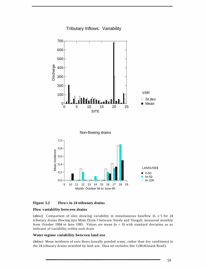
59
Tributary Inflows: Variability
0 5 10 15 20 25SITE
0
100
200
300
400
500
600
700
Dis
char
ge
MeanSt.dev
VAR
Non-flowing drains
9 10 11 12 13 14 15 16 17 18 19
Month: October 94 to June 95
0.0
0.2
0.4
0.6
0.8
1.0
Mea
n in
cide
nce
br-100br-50h-50
LANDUSE$
Figure 3.2 Flows in 24 tributary drains
Flow variability between drains
(above) Comparison of sites showing variability in instantaneous baseflow (L s-1) for 24tributary drains flowing into Main Drain J between Yenda and Yoogali, measured monthlyfrom October 1994 to June 1995. Values are mean (n = 9) with standard deviation as anindicator of variability within each drain
Water regime variability between land use
(below) Mean incidence of zero flows (usually ponded water, rather than dry conditions) inthe 24 tributary drains stratified by land use. Data set excludes Site 3 (McKissack Road).

60
Conductivity
9 10 11 12 13 14 15 16 17 18 19Month: October to June
0
2000
4000
6000
Con
duct
ivity
Turbidity
9 10 11 12 13 14 15 16 17 18 19Month: October to June
0
20
40
60
80
100
NT
U
Suspended Sediment
9 10 11 12 13 14 15 16 17 18 19Month: October to June
0
100
200
300
400
500
mg
L-1
Total Phosphorus
9 10 11 12 13 14 15 16 17 18 19Month: October to June
0.0
0.5
1.0
1.5m
g L-
1
Figure 3.3 Seasonal trends in water quality
Seasonal trends in water quality and its variability shown using a box-and-whisker plot,showing median (the mid line inside the box) with the box enclosing the central 50% ofvalues. Restricting the y-axis in order to emphasise the width of the ‘box’ means someextreme values are not shown on the graphs (see text).
Continued on next page.

61
Organic (TKN) Nitrogen
9 10 11 12 13 14 15 16 17 18 19Month: October to June
0
2
4
6
8
10
mg
L-1
Oxidised (NOx) Nitrogen
9 10 11 12 13 14 15 16 17 18 19Month: October to June
0
2
4
6
8
10
mg
L-1
Total Nitrogen
9 10 11 12 13 14 15 16 17 18 19Month: October to June
0
5
10
15
20
mg
L-1
Figure 3.3 (contd.)

62
Conductivity
9 10 11 12 13 14 15 16 17 18 19Month: October to June
0
1000
2000
3000C
ondu
ctiv
ity (
mic
roS
cm
)
Suspended Sediments
9 10 11 12 13 14 15 16 17 18 19Month: October to June
0
50
100
150
200
250
SS
(m
g L)
Total Phosphorus
9 10 11 12 13 14 15 16 17 18 19Month: October to June
0.0
0.05
0.10
0.15
0.20
0.25
Tot
al P
(m
g L)
Total Nitrogen
9 10 11 12 13 14 15 16 17 18 19Month: October to June
0.0
2.5
5.0
7.5
Tot
al N
(m
g L)
Figure 3.4 Tributary water quality: Seasonal patterns by land use
Seasonal trends from October 1994 to June 1995 in conductivity, suspended sediments, totalphosphorus and total nitrogen for three land use types: BR-100 shown as solid circle, BR-50shown as hollow circles, and H-50 shown as solid squares.

63
LOAD: Organic Nitrogen
9 10 11 12 13 14 15 16 17 18 19
Month: October 94 to June 95
0
10
20
30
40
kg p
er d
ay (
mea
n pe
r dr
ain)
LOAD: Suspended Sediment
9 10 11 12 13 14 15 16 17 18 19
Month: October 94 to June 95
0
500
1000
1500
2000
kg p
er d
ay (
mea
n pe
r dr
ain)
LOAD: Total Nitrogen
9 10 11 12 13 14 15 16 17 18 19
Month: October 94 to June 95
0
25
50
75
100
kg p
er d
ay (
mea
n pe
r dr
ain)
LOAD: Total Phosphorus
9 10 11 12 13 14 15 16 17 18 19
Month: October 94 to June 95
0
1
2
3
4
5
kg p
er d
ay (
mea
n pe
r dr
ain)
LOAD: Oxidised Nitrogen
9 10 11 12 13 14 15 16 17 18 19
Month: October 94 to June 95
0
25
50
75
100
kg p
er d
ay (
mea
n pe
r dr
ain)
Figure 3.5 Seasonal loads for types of land use
Seasonal pattern of loads of suspended sediment, total phosphorus and forms ofnitrogen under low-flow conditions in each month from October to May 1995 shownas mean load (kg day-1) per drain, for each land use type. June is not includedbecause of the small sample size. Error bars are not shown for clarity, but there isconsiderable range in values for all months and land uses.

64
Chapter 4Chapter 4
High Flows and Rainfall EventsHigh Flows and Rainfall Events
4.14.1 Rain, high flows and water qualityRain, high flows and water qualityThe load of soluble and particulate nutrients exported during a flood can be verylarge, and may be a significant proportion of total annual export. Although highdischarge dominates loads, it can have a diluting effect on nutrients (eg Hart et al.1988). When the Herbert River, Queensland, flooded in January 1994, the highestconcentration of particulate phosphorus was 200-250 µg L-1 (Mitchell et al. 1997);however, net export was 600 t nitrogen, 65 t phosphorus and 100,000 t suspendedsediment.
Measurements defining hydrograph shape as well as peak discharge are essential inorder to achieve accurate estimates of loads. In turn, accurate estimates of nutrientexport during flood events need to recognise that nutrient concentrations do changeduring flood events. Rising and falling hydrographs can have distinctive waterquality composition (eg Mitchell et al. 1997) and, more importantly, peaks indischarge and nutrients rarely coincide and are more typically offset (Walling andWebb 1996). During a flood event on the Murrumbidgee River at Narrandera, NewSouth Wales, the sediment peak preceded the discharge peak by about 4 days (Oliveet al. 1996).
Only a few studies have documented water quality changes during flood events forAustralian creeks or rivers. Results are mixed, thus there is no general pattern. Forexample, during floods, the Magela Creek system, showed a two-fold dilution ofmajor ions but a six-fold increase in suspended sediment (Hart et al. 1988). On theMurrumbidgee River, sediment concentrations on the rising hydrograph initiallyincreased then decreased, and were much lower on the falling hydrograph (Olive etal. 1996). Because of the differences between rise and recession, special sampling isneeded and different routines are used. Thus Olive et al. (1996) sampled at 6-hourlyintervals for 12 days, whereas Hart et al. (1988) sampled five times on the rising limband five on the falling limb of a 30-hour long flood on the Annan River, Queensland.Automatic sampling triggered by changes in water level was used to collect watersamples from a wetland constructed on a natural drainage line in northern Victoria(Raisin et al. 1997).
As far as can be determined, there have been no studies of changes in quality ofirrigation drainage water during high flows. Monitoring tends to be compliance-oriented and routine rather than event-driven, and focus on concentration ratherthan loads. Subsequent reports do not identify samples affected by rainfall (egMcKay et al. 1988, Shepheard 1994).
Reasons for the variable water quality during high flows are that as well as dilutingbaseflow, a heavy rainfall can indirectly alter the composition of water quality if theresulting discharge erodes, entrains, or transports solutes or particles. On theAnnan River, all these occurred: rain diluted the baseflow of major ions at a lowersite but further upstream there was evidence of material being flushed in (Hart et al.1988). It is because rainfall is such an important factor influencing exported loads,

65
that wet, dry and average scenarios are used, for example when modelling annualnutrient exports in the main rivers of the Murray-Darling Basin (GHD 1992) or forcomparing longitudinal trends down the River Murray (McKay et al. 1988).
In terms of understanding the effects of rainfall on discharge, irrigation areas differfrom natural catchments in the following very important respect: run-off is notdependent on rainfall. Instead it can also occur as a result of water management,whether by the farmer (ie irrigation run-off) or by the water management authorityor agency (discharging water directly through the system, etc). In general, it isirrigation run-off that has attracted most attention in water quality monitoringprograms and investigations (eg Harrison 1994) and the importance of these otherfactors is overlooked. The emphasis of compliance monitoring has been onconcentrations (see Harrison 1994) and this has drawn attention to sources ofnutrients in drainage water, rather than to the loads exported. Thus the importanceof rainfall in determining quantities of nutrients exported in irrigation drainagewater is not much considered.
Although irrigation areas can be considered as a set of small catchments (Chapter 2)and are often studied that way (eg Tiwari 1994), the catchment model must be usedwith caution. Not only is run-off independent of rainfall, but irrigation catchmentsdiffer from natural catchments in other ways: they are not bounded by points ofhigh relief but by constructed water delivery systems; the landscape selected forirrigation usually has a very gentle slope hence run-off is unlikely to be rapid andscouring as in an upland catchment; under irrigation, water is applied according tospecific plant needs so generates a more predictable run-off than in naturalcatchments where rainfall may be patchy and variable.
Pathways to irrigation drainsPathways to irrigation drainsAfter rainfall, the water in irrigation drains is a mix of agricultural and non-agricultural sources, such as (depending on locality) urban run-off, rain rejectionflows and tile drainage. The relative importance of these has not been specificallymeasured but is known, approximately, for the Mirrool Irrigation Area from back-calculations (Tiwari 1994):
As percentage of annual total discharge
Farm drainage 41%
Ground water pumping 2%
Town drainage 2%
Non-irrigation area run-off 8%
Escape water 47%
These sources can be expected to have different water quality signatures and sources(Table 3.5) and these may reach the main exit drain at different rates and in differentsequences. For example, discharge from tile drains may be the slowest to reachlateral and trunk surface drains, as rainfall must first percolate through the soil thenaccumulate at the sump before being pumped into drains.
Another aspect of the heterogeneous nature of irrigation drainage is that neither thequantity nor quality of agricultural run-off is fixed. Quantity will vary depending

66
on the time of year, whether in the irrigation season or not, and if in the irrigationseason, it depends on phenological stage of the crop and whether water is needed ornot. As a generalisation, rain is free water for irrigation farmers during theirrigation season so if it rains water orders may be cancelled. The ordered, butunwanted, water is carried in supply channels as rain rejection water, and isdischarged directly into the drainage system via escapes (Chapter 1.4). The releaseof rain rejection water may last a few to several days, until the unwanted water hasbeen re-routed, and is influenced by the length of the main supply channel. Thismay be already holding sufficient water for a few days when the cancellation ordersare received. In the MIA, supply channel length is quite long. The Main Canal atGriffith is nearly 160 km from its diversion point out of the Murrumbidgee River.Rejected water from the MIA can be stored in Barrenbox Swamp (Lillian Parker,pers. comm. 1998).
Crop type, stage and drainage dischargeCrop type, stage and drainage dischargeCrops have specific water requirements and watering schedules. Crops that areirrigated, such as permanent plantings are irrigated at intervals throughout thegrowing season. In contrast rice is grown in large bays and it is only at certain timesof the irrigation season that large quantities of water are required. Thus the patternof agricultural drainage from these two crops varies.
The quantity of run-off, as a result of rainfall, from a rice crop that reaches a draindepends on crop stage, on the cultural practices of the grower and on the size of therainfall event. Note that since this project was done, there has been a change andfarmers are now required to retain the first 12 mm of rainfall run-off on-farm.Previously, under some circumstances, even a small rainfall would have resulted inrun-off or discharge to farm drains, and hence to irrigation drains. This would haveoccurred almost immediately and continued until the excess water in the bays wasdischarged. However, if rice bays were not full, that is if there was “free space” inthe bays, then run-off or deliberate releases by the rice-grower would happen only ifrainfall is heavy and sustained. Understanding drainage in the MIA, or other rice-growing areas, requires detailing its irrigation requirements at different growthstages.
A generalised run-off calendar for Mirrool IA is set out below, applicable to theearly-mid 1990s.
Run-off calendarRun-off calendar♦ Early in the growing season (September-October), there is a demand for
irrigation water to fill (to a required depth) rice bays prior to sowing. Rainfall iswelcomed and used. Agricultural run-off in the drains comes from citrus andvines, if irrigation has started early, or from filled bays, as well as from rainrejection flows.
♦ In mid-season (November-December), once the seedlings have established, thewater in the rice-bays is made deeper and held there prior to panicle initiation,so rain during the deepening stage is welcome but less so afterwards. Bays maybe locked up for 21 days during weed control. As for the earlier stage,agricultural run-off in the irrigation drains comes from citrus and vines, andfrom rain rejection flows.

67
♦ Once the rice crop is established, the bays are kept relatively deep with stablewater levels (December-January) to buffer against temperature changes.Summer rainfall, which can be as heavy storms, tends to be unwanted and mayforce deliberate releases as well as run-off. Run-off to drains comes from ricebays, citrus and vine crops, row crops and from rain rejection flows.
♦ Once the rice has flowered and been fertilised, water in the ricebay is allowed tofall, a stage known as ‘locking up’ the bay (January-April). Rainfall is notwanted as this can prevent the soil drying out to firmness enough for heavymachinery. Rain therefore results in immediate run-off.
♦ Once the harvest is completed, and outside the irrigation season (end of May toSeptember), the irrigation season is over, for rice and other crops (unlessexceptionally dry). Water in the Main Canal is now meeting only urban andlimited Stock and Domestic needs. If rain falls, it is not needed so runs off.Seepage may activate tile drainage pumps. There is no rain rejection or escapewater.
Aims and objectivesAims and objectives The principal aim was to estimate the importance of nutrient loads during rainfall-induced flow-events and to describe changes in water quality at different stages inthe hydrograph, as per Experiment 3 (Appendix A). Loads could not be calculatednor could the rising and falling limbs of the hydrograph be identified due to lack ofdischarge data (see below). However, intensive water quality sampling was doneallowing two hypotheses to be critically explored.
♦ First, that a rainfall event of a given size will result in run-off in irrigation drains,of variable quantity depending on time of year.
♦ Second, that quality of drainage water during a rain event will be heterogeneous.
For the first, the null hypothesis was explored by comparing hydrographs afterrainfall, using historical flow data for Main Drain J and by selecting rainfall events atdifferent times of the year. The assumption was that the relationship betweenrainfall and drainage would be modified because of responses to different crops andto crop stage. Only five events were analysed.
For the second, the null hypothesis was that drainage water quality ishomogeneous, at least in the short term (eg every six hours). This was explored bycomparing water quality changes through time. Data were collected by monitoringvariations in nutrient concentrations during a rainfall event.
The site chosen was close to the Yoogali gauge, as it was expected that dischargedata collected routinely by the former NSW Department of Water Resources wouldallow calculations of loads. An additional advantage was that the site was close tothe laboratory, giving a quick response and easy maintenance of the autosampler.
4.24.2 MethodsMethods
Hydrograph comparisonsHydrograph comparisons Five hydrographs associated with specific rainfall events for Main Drain J at YoogaliGauge (Number 410150) were chosen to cover different stages in the year: spring,

68
summer, late summer, autumn and winter. All hydrographs were selected from1992-1993 in order to be as close as possible to contemporary conditions.
The catchment above Yoogali gauge is a mixture of broadacre (rice, pasture) andhorticulture (predominantly citrus and grapes), and includes four villages (Yenda,Yoogali, Beelbangera and Bilbul) as well as part of the Griffith suburban area(Figure 2.2, Table 3.1). Discharge data were provided by the Tumut office of theformer NSW Department of Water Resources. Rainfall records for Griffith wereprovided by the Griffith laboratory of CSIRO, an official Bureau of Meteorologyweather station.
It was expected that isolated rainfall events would give the clearest comparisonbetween seasons. Accordingly the following criteria were set: the rainfall eventshould be 15-20 mm and fall within one 24-hour period, with ‘no’ rain (<0.35 mm) inthe 4 preceding days, and ‘no’ (ie <0.35 mm) rain in the following 7 days. Thesecriteria proved too stringent, partly because of the patchy flow records. A searchthrough six years of rainfall data (Excel macro, Michael Reed, CSIRO) found only 24rainfall events that met these criteria between 1 January 1988 and 31 December 1993,and of these only 12 had matching discharge data. These twelve were not spreadwell through the year. At least 5 coincided with the onset or end of the irrigationseason, when water levels are changing rapidly, making interpretation ofhydrographs difficult. The final criteria are more relaxed but still identify isolatedevents (Table 4.1).
Comparison between hydrographs is graphical. All plots show a day of substantiverainfall (Day 0), as well as rainfall and discharge for the 5 days preceding and 7 dayssubsequent.
Water quality monitoring and comparisonWater quality monitoring and comparison Field set-up An automatic sampler was set up at a site 200 metresdownstream of the Yoogali gauging station, which was 150 metres downstream ofany input to Main Drain J. This was chosen on the assumption that the watercolumn was well-mixed.
Intensive monitoring was completed on three occasions, but only two were rainevents. Dates and rainfall are summarised in Table 4.2. The choice of dates waslimited by the need to coincide availability of an auto-sampler and a rainfall event,with field staff. Field staff and field equipment were involved in other water qualityresearch projects and were not always available at the short notice (less than 24hours, between onset of rain and rising hydrograph: see Figure 4.1) needed torespond to a rainfall event.
Automatic samplers Samples were taken from the water column using aManning Model 4040 auto-sampler set to deliver 250-300 mL sub-samples at pre-determined intervals, ranging from 30-60 minutes (Table 4.2). Samples wereseparately delivered into acid-washed 300 mL bottles, either HDPE or glass bottles.Samples were collected from a fixed depth (eg 400 mm) below the water surface,throughout a particular event.
Sample processing and nalyses Samples were collected at ambient temperatureand removed from the auto-sampler within 9 hours and stored at 4oC prior toprocessing and preparation for chemical analysis. Processing was carried out within48-60 hours. Samples were filtered then frozen prior to NOX or FRP analysis, and asub-sample taken at the same time was placed in a digestion tube for TP and TKN

69
analysis. Details of physico-chemical and chemical methods are described inAppendix D, and abbreviations used previously are used henceforward.
Discharge Discharge data for Yoogali gauge were not available (Chapter 1.4).The possibility of using an alternative station downstream on Main Drain J wasexplored. The closest gauging station, Warburn Escape GS 410055, was unlikely toreflect discharge behaviour at Yoogali gauge because it receives supply water fromthe Mirrool area and from Warburn Escape. In addition, its discharge was notcontinuous. Hence, no nutrient loads were calculated.
4.34.3 ResultsResults
Hydrograph comparisonHydrograph comparison Spring Rainfall of 12.7 mm fell on 24th October 1993 (Figure 4.1). Dischargein Main Drain J which had been approximately 110 ML d-1 for the four precedingdays, increased by 10-15 ML d-1 or by 9-14% in the two days immediately afterwardsthen fell, stabilising at 105 ML d-1 by Day+4.
Thus the effect of this spring rainfall was an immediate (ie within one day) butminor (10-15 ML increase) and short-lived (only 2 days) increase in discharge inMain Drain J.
Summer Rainfall of 26.4 mm fell on two days in February 1993 (Figure 4.1),with 5.3 mm on the first day and 21.1 mm on the second. Discharge, which in thepreceding 4 days had ranged from 195-217 ML d-1, increased immediately from 205ML d-1 on Day 0 to 253 ML d-1 on Day+1 after only 5.3 mm rain. This was anincrease of 23% (48 ML d-1). Discharge increased again after a further 21.1 mm rainon Day+1 reaching 310 ML d-1 on Day+2. This was an increase of 22% from Day+1to Day+2. Thereafter drainage discharge remained high and did not return to 195-217 ML d-1 range until Day+11 (not shown). The return time was lengthenedbecause further rainfall of 12.7 mm on Day+5 resulted in an immediate increase indrainage from 250 to 324 ML d-1, an increase of 30% (74 ML).
Thus rainfall of 26.4 mm in summer resulted in an immediate (Day+1) and majorincrease (22-30%) in drainage. Unlike in spring, the return to pre-rainfall dischargelevels took longer than 4 days, as shown by elevated discharge on Day+5, and waspostponed by further rain on Day+5.
Late Summer Rain, 27.7 mm, fell on 6th March 1993 followed by 12.7 mmtwo days later (Figure 4.1). Discharge in Main Drain J, which had been rangingfrom 252-272 ML d-1 in the four preceding days, increased rapidly from 260 ML d-1
on Day-1 to 327 on Day 0, reaching 502 ML d-1 on Day+1, an increase of 93% (242ML), then decreased. Rainfall of 12.7 mm on Day+2 prevented drainage fromdecreasing any further and instead it increased again from 379 ML d-1 to 406 ML d-1
on Day+3, a 7% increase (27 ML). Drainage discharge returned to pre-rainfall levelson about Day+6. The increase in discharge from Day-1 to Day 0 suggests a pre-release.
This Late Summer hydrograph is similar to the Summer hydrograph. In response torain, there was an immediate (1 day or less) and large (93%) increase in drainageand the return to pre-rainfall discharge levels were postponed by follow-up rain, inthis case only 2 days later.

70
Autumn Rainfall of 13.5 mm fell on 26 May 1992. Discharge in Main Drain J,which had been 84-92 ML d-1 in the preceding five days (Figure 4.1), increasedimmediately and peaked the following day at 124 ML d-1, an increase of 32 ML d-1
(35%). Unlike the two Summer hydrographs which showed sharp peaks, theautumn hydrograph was relatively flat. It was also quite short, lastingapproximately 2 days only before returning to pre-rainfall levels, and in this it wassimilar to the Spring hydrograph. The very rapid response to autumn rainfall isevident in the discharge increase (Figure 4.1) at Day+7.
This Autumn hydrograph shows that drainage response to rainfall was immediate(within 1 day) even at the close of the irrigation season, and resulted in a largeabsolute (32 ML) and relative increase in discharge.
Winter Rainfall of 19 mm on Days 0 and +1 (Figure 4.1) on 18th and 19th July1992 produced a hydrograph quite distinct from Spring, Summer, Late Summer andAutumn ones. Discharge, which prior to this rain had been only 0.06-0.11 ML d-1,rose to 0.5 ML d-1 on Day+1 then to 1230 kilolitres ML d-1 on Day+2, then decreased.Despite no further rain, there was a second major discharge peak of 2.84 ML d-1 onDay 4, and a third major peak of 1.3–1.8 ML d -1 on Days+8 to +10 (not shown).These second and third peaks are interpreted as late arrival of run-off from furtherup the catchment, with the most likely source being the large area north of Bilbuland Yenda (Figure 2.2). These delayed peaks are not obvious during the irrigationseason, possibly because they are obscured by the much higher base flows.
The Winter responses differed from the other seasons in being slower to reach apeak (1, 2 or even 3 days) and in having multiple peaks. The increase in drainagewas large relative to preceding flows, but quite small in absolute terms. This rainfallof 21.3 mm, spread over 4 days (Figure 4.1) resulted in a net increase of first 1 then2.5 ML d-1 which was considerably less than the others examined. Being outside theirrigation season, it is probable that this small increase represents actual run-off fromthe catchment.
This brief analysis of rainfall and flow records, summarised below (Table 4.2), showsthe significance of time of year in determining the quantity of drainage. Althoughthe discharge resulting from a rainfall event is quite variable through the irrigationseason, it was considerably more than outside the irrigation season. A rainfall of 12-14 mm resulted in a discharge increase of 10-15 ML (Spring), 74 ML (summer), 27ML (late Summer) and 32 ML (Autumn) whereas a larger rainfall, of 21.3 mm, inWinter resulted in approximately only 3.5 ML drainage increase. Hence the highflows resulting from 12-25 mm rainfall events are composed of water other than run-off and are a consequence of water management practices.
Water quality comparisonWater quality comparison
Event Event 1 18th and 19th January 19941 18th and 19th January 1994 Sampling followed very light rainfall (0.3 mm on 17th January 1994) which was thefirst since 28 December 1993. There was no follow-up rain despite the threateningappearance of the weather. Lack of rain means this run of 24 samples can beconsidered as a background record of water quality in midsummer (Figure 4.2).
It is noticeable that, even in the absence of a rain event, the water quality of drainagewater was not constant. The six measures of water quality showed different trendsthrough the 24-hour sampling period. EC showed two peaks, of 0.66 and 0.60 mS

71
cm-1, after 4 and 15 hrs respectively had elapsed since sampling began. Turbidityvaried little, remaining at or close to 40 NTU throughout the 24-hour periodalthough there was a decrease at hours 3-6. SS oscillated around 100 mg L-1 for mostof the 24-hour sampling with an increase at 22-24 hours. TKN peaked at 0.66 mg L-1
after 6 hours, then decreased steadily reaching 0.4 mg L-1 after 18 hours. NOx wasthe most variable parameter, ranging from 0.9 to 1.7 mg L-1. The two NOx peaks, at3-4 hours and at 15 hours, broadly coincide with EC peaks. The first coincided withlower turbidity which may have been caused by salinity-induced flocculation. Thesetwo EC and NOx peaks probably originate from tile drainage sumps.
Event Event 2 11 July 19942 11 July 1994 Thunderstorms during the night of 10-11th July 1994 were followed the nextmorning with a shower (4 mm) at 0900 on 11th July 1994. The auto-sampler wasrapidly installed. Sampling began at 0930 h and lasted 9 hours. There was arelatively severe thunderstorm (6.1 mm) at about 1100 hours. Water depth on thereference pole was 296 mm above intake when sampling began (0930 h) and 280 mmwhen it finished (1825 h) indicating a net reduction in discharge over the 9-hoursampling period.
The four water quality parameters again showed different trends through time(Figure 4.3). EC decreased slowly from an initial value of 0.46 to 0.31 mS cm-1 after7.5 hours then increased. Turbidity was generally about 30 NTU except for twopeaks of 43 and 37 NTU after 1.5 and 7 hours respectively. The first peak coincidedwith a rainstorm. TP increased slightly soon after sampling started, reaching a peakof 0.39 mg L-1 after 1.5 hours and was then stable at 0.36 mg L-1. NOx was initially>0.3 mg L-1, but declined throughout the 9-hour sampling period to 0.08 mg L-1 after8.5 hours. NOx decreased rapidly for the first 3 hours, then slowed.
Several inputs appear to have occurred in this time frame, each with different effectson water quality. The initial increase in turbidity coincided with the late morningrainstorm, and was probably due to either immediate run-off into Main Drainand/or benthic sediment being entrained by rapid (presumed) increase in discharge.Consistent with this is the small increases in TP and NOx. A delayed run-off,possibly entering Main Drain J further upstream or from a larger catchment, issuggested by the second peak in TP, turbidity and EC. Another type of input isindicated by EC and NOx, with decrease suggesting dilution and increasesuggesting a pulse of tile drainage. Without discharge data, the changes are difficultto interpret.
Event Event 3 17th-18th May 19953 17th-18th May 1995 Steady rain fell from 0300 to 1200 hours on the 17th May 1995. An auto-sampler wasinstalled at 1040 hours and the first sample was at 1110 hours, and continued at 30minute intervals. By 1610 hours, there had been over 10 mm of rain. At 1610 hours,the sampling interval was altered and a sixty minute interval selected so as tocontinue overnight unattended until 0830 on 18th May. There was further light rainfrom 1830 to 2200 hours (>3 mm). Discharge in Main Drain J at station furtherdownstream (Warburn Escape) was about 150-200 ML d-1.
As with the two previous intensive samplings, water quality varied through the 21-hour sampling period (Figure 4.4). Initial values of EC, turbidity, TKN and NOx inwinter 1995 were considerably higher than in Events 1 or 2 in 1994.

72
EC increased rapidly after sampling started, reaching 0.91 mS cm-1 at 2-3 hours,decreased to 0.70 mS cm-1 at 8.5 hours, and from then to end of sampling period wasfairly constant at 0.72 mS cm-1, with a small peak at 16.50 hrs. Turbidity increasedsteadily from 87 NTU reaching 219 NTU at 13.30 hrs after the start. There was avery high value of 280 NTU at 7.5 h. TP remained low in the range 0.10-0.19 mg L-1
for the first six hours then increased rapidly to 0.54 mg L-1 at 9.5 hrs, then decreasedstabilising at about 0.3 mg L-1 from 15.5 hrs. TKN increased erratically reaching 3.06mg L-1 after 9.5 hrs, coincident with the TP peak, then decreased to 1.8-2.1 mg L-1,which was still fairly high. NOx rose slightly to 2.4 mg L-1 at 5 hrs, then decreaseduntil 9 hrs, increased to 14-15 hrs then decreased again.
Two patterns are evident in this rain event. Concentrations of TP, TKN andestimates of turbidity, which were all high initially, increased even further duringinitial sampling and 9 hours later were 5, 4 and 2-3 times higher than whensampling began at 1110 hrs. This coincided with another rainfall event.Entrainment of lateral and benthic sediments, road run-off and scouring probablycaused these increases. In contrast, concentrations of EC and NOx went throughincrease and decrease cycles, but by the end of the sampling period were reduced byabout 15% of their starting value. Changes in EC and NOx were probably due todischarging tile drain pumps (increase) and increase in escape or run-off (dilutioneffects).
All EventsAll Events Comparisons of water quality during the three events (Table 4.4) with long-termrecords for Main Drain J (Shepheard 1994) show that:
♦ In Event One, during the irrigation season: EC was generally high relative tolong-term but turbidity and TP were lower
♦ In Event Two, outside the irrigation season: EC and turbidity were lower thanexpected for winter
♦ In Event Three, outside the irrigation season: turbidity was higher, exceptionallyso.
Compared with Harrison’s ranking (Chapter 3.2), the concentrations of TP, TN andNOx were ranked as Medium. During winter event (Figure 4.3), TP was Mediumand NOx was Low. During the autumn event (Figure 4.4), TP was Medium butNOx and therefore TN were medium, verging on High, with no evidence ofdilution.
4.44.4 DiscussionDiscussion
Rainfall and dischargeRainfall and discharge At all times during the year, and for whatever reason (direct run-off and/or rainrejection or rain pre-release), rainfall was followed by an immediate increase indrainage discharge. The size of this increase was consistently greater during theirrigation season than in winter.
Historical data for the Yoogali gauge at Main Drain J, which is an SO4, showed thata rainfall of 20-30 mm during the irrigation season resulted in an increase of 67-242ML d-1, or a 22-93% increase in discharge (Table 4.3). A similar-sized rainfall outsidethe irrigation season caused an increase in discharge of only 3.5 ML. Higher up the

73
catchment, in drains of lower order, this irrigation-induced effect is even morenoticeable. Tiwari (1994) working on rice sub-catchments south of Griffith, observedthat 20 mm rainfall resulted in run-off yield of 1 ML d-1 per 1000 ha during winterbut that in summer this rose to 14 ML d-1 per 1000 ha. This discrepancyimmediately raises questions about different water qualities. Obviously, during theirrigation season discharge in irrigation drains is composed of much more thanrainfall run-off, and sampling should be focused on this.
Equally obviously, estimates of nutrient loads based on one water sample or takenfrom the hydrograph peak will give inaccurate estimates of load. Future waterquality monitoring will need to be much more intensive in order to estimate highflow loads and may have to continue well beyond the flood peak in order toadequately sample water quality during flood recession. In Mirrool, at least, thisreceding limb appears to be surprisingly long: up to 5 days during the irrigationseason and possibly 11 days during winter. Such long recession limbs may haveimplications for monitoring other aspects of water quality, such as pesticides.
Several factors influence discharge quantity and timing, and there are even moreduring the irrigation season. In horticultural areas, for example, the list of factorsincludes: drainage density is high (Table 2.2), rainstorms particularly in summermay be intense but often localised, catchments are variable in shape and size, watermanagement by the water authority and its operators, water management by thefarmer. Because these can act synergistically or in sequence, flood hydrographs inintensely used irrigation areas such as Mirrool are likely to be highly variable inshape and size, and possibly not readily predictable.
The intensive sampling done in Main Drain J lasted only up to 24 hours. At thetime, this was thought adequate to capture the flood response but in retrospect it isevident that this was not adequate to fully characterise flood recession. On rivers,the receding limb is affected by floodplain returns. In irrigation areas, theequivalent is the distant sub-catchments and tile drainage. On-farm investigationsof tile drain effectiveness in the Mirrool Irrigation Area suggest that tile drains cantake from 8 to 13 days to lower the water table to below 1 metre after irrigation,rather than the 3 days they were designed for (Muirhead et al. 1994). If this delay iscommon, then in a period of heavy rain, tile drains will be discharging into drainsfor several days after rain has stopped, with consequences for water qualitysampling. This justifies the low-flow sampling strategy used in the Trunks andTribs Study (Chapter 3) and the concern to sample away from the influence ofrainfall events (Chapter 3).
Water quality variabilityWater quality variability Event One, when rain did not result as expected, was useful in showing the extent ofnormal variability through 24 hours in summer. Even under these conditions, onlysome water quality measures remained fairly constant. EC, SS and TP all stayedwithin a defined range. Nitrogen, however, was much more variable (Table 4.4) andhence potentially a much greater source of error for load calculations. The smallspikes of EC and NOx are typical of tile drainage (see H-50 mean water quality inTable 3.5). These small but concentrated discharges into Main Drain J were alsonoted by Bowmer et al. (1992), and show that slugs of water can move through thesystem. In turn, this challenges the assumption of homogeneity regarding thelocation of the autosampler. Specific sampling would be needed to determine if

74
these spikes were the result of incomplete mixing or in fact signalled fluctuations inwater quality.
This highlights a very real and basic problem in water quality monitoring inirrigation areas. The number of lateral drains is high, particularly in horticulturalareas such as Mirrool. In addition, there are many direct inputs (eg Chapter 3.2),although not all are known or approved.
The two events outside the irrigation season, Events 2 and 3, with 10.3 and 14.5 mmrain respectively, were quite different in character. Event 2 was a short, heavyrainstorm and Event 3 was prolonged rain. Event 2, being more intense, was morelikely to generate erosive runoff. The variable record and the sudden peaks inturbidity (Figure 4.3) suggest that runoff did happen, but not to a great extent, interms of the water quality. Absolute values were not high, being similar tobackground values in Event 1. In contrast, the less intense but longer-lasting rain inEvent 3 resulted in a steady increase in turbidity, to more than 200 NTU. Thesevalues were exceptionally high for Main Drain J. Possible explanations are thatflows scoured loose materials following drain maintenance, or channel-forming, or aconsequence of major land use changes in the catchment, for example, the expansionof wine-grape plantings. The long-term record for a site further downstreamreported no values greater than 200 NTU between 1978 and 1993 (Shepheard 1994).
During a flow event, the increase in water velocity past a critical threshold inrelation to residence time (Harris 1996) signals a change in the dominant processes.With sediments, for example, this shift means that scouring and entrainment replacedeposition. Effectively, a flood event changes a channel from being a sink to being asource. Determining which are the dominant processes, the switching point, andtheir duration is an essential step in making a prognosis of wetland ‘performance’(Raisin 1995). In Event Three, there was some evidence of this shift. The highturbidity values suggested both wall scouring and loose benthic materialentrainment. The low relationship between turbidity and TP suggested sub-soilscouring, and increasing TKN suggests entrainment, or eleution.
A number of processes are indicated, and thus the expectation of hysteresis in waterquality in drains, as in rivers, during a rising versus a falling hydrograph is unlikelyto be true for SO3 and SO4 drains within the irrigation area. Sampling furtherdownstream where inputs are mixed, ie well down an exit drain, or above inputs, iein SO1 drains, will remove some of the fluctuations in the data.
Without discharge data, these interpretations can only be tentative. Dedicatedstudies would be required to establish firmly the importance of rainfall events insummer to nutrient export load from the MIA, and to determine the relativeimportance of agricultural run-off versus escape and rain rejection water as a drivingfactor, for example in relation to entrainment and re-suspension.
FindingsFindings The two null hypotheses, of uniformity in drainage discharge and homogeneity inwater quality as a response to rainfall, were considered invalid. There was someevidence, and considerable likelihood, that because irrigation areas are so intenselymanaged, this could increase the heterogeneous element in drainage responses, inboth quantity and quality. This has serious implications for calculating nutrientloads.

75
♦ Frequent sampling, including beyond the obvious hydrograph peak, isnecessary to define the hydrograph and to collect water samples.
♦ Most of the high flows resulting from small to medium rainfall events during theirrigation season are a consequence of land and water management practices.
Irrigation areas with complex drainage networks and diverse and changing landuses will have variable responses. Rainfall-related discharge responses may take 5to 11 days to pass a given gauging station, depending on sub-catchment sizes. Thusthe end of flood recession may pass unnoticed during the irrigation season, beingmasked by the high flows normal for that time of year
♦ Single samples during flood passage or taken at the flood peak are totallyinadequate, as they are in rivers. Because of the number and diversity of inputs,nutrient concentrations change independently of each other.
ReferencesReferencesBowmer, K.H., Bales, M. and Roberts, J. (1992). The effect of aquatic plants on water quality in
irrigation drains: a feasibility study for the Murray-Darling Basin Commission. CSIROConsultancy Report 92/17. CSIROP Division of Water Resources, Griffith.
GHD (1992). An investigation of nutrient pollution in the Murray-Darling River system. Reportprepared by Gutteridge, Haskins and Davey, for the Murray-Darling BasinCommission.
Harris, G.P. (1996). Catchments and aquatic ecosystems: nutrient ratios, flow regulation andecosystem impacts in rivers like the Hawkesbury-Nepean. CRC Freshwater EcologyDiscussion Paper, June 1996.
Harrison, J. (1994). Review of nutrients in irrigation drainage in the Murray-Darling Basin.CSIRO Division of Water Resources. Seeking Solutions. Water Resources Series:No 11.
Hart, B.T., Day, G., Sharp-Paul, M.A. and Beer, T. (1988). Water quality variations during aflood event in the Annan River, north Queensland. Australian Journal of Marine andFreshwater Research 39:225-243.
McKay, N., Hillman, T. and Rolls, J. (1988). Water Quality of the River Murray: Review ofMonitoring, 1978-1986. Water Quality Report No. 1. Murray-Darling BasinCommission, Canberra.
Mitchell, A.W., Bramley, R.G.V., and Johnson, A.K.L. (1997). Export of nutrients andsuspended sediment during a cyclone-mediated flood event in the Herbert Rivercatchment, Australia. Marine and Freshwater Research 48:79-88.
Muirhead, W.A., Tijs, S. and Sinclair, P.J. (1994). Tile drain performance in MIAhorticultural farms. Farmers Newsletter 174: 29-31.
Olive, L.J., Olley, J.M., Wallbrink, P.J. and Murray, A.S. (1996). Downstream patterns ofsediment transport during floods in the Murrumbidgee River, NSW, Australia. Z.Geormorph. N.F. Suppl.-Bd.105: 129-140.
Raisin, G.W. (1995). The management of non-point source pollution in rural catchments. FinalReport. Project M202, Natural Resources Management Strategy.
Raisin, G.W., Mitchell, D.S. and Croome, R.L. (1997). The effectiveness of a smallconstructed wetland in ameliorating diffuse nutrient loadings from an Australianrural catchment. Ecological Engineering 9:19-35.

76
Shepheard, M. (1994). Murrumbidgee Irrigation Area: Surface Water Quality Project. TechnicalReport No. 94/07.
Tiwari, A. (1994). Murrumbidgee Irrigation Area Farm Drainage investigations. TechnicalReport No 94/06. Technical Services. Murrumbidgee Region. NSW Department ofWater Resources.
Walling,, D.E. and Webb, B.W. (1996). Water quality. I. Physical characteristics. In: G. Pettsand P. Calow (eds.) River flows and channel forms. Blackwell Science, Oxford.

77
Table 4.1 Sampling details for comparison of hydrographs
Dates and antecedent conditions for the five rainfall events used in the hydrographiccomparison of drainage discharge.
Season Actual dates Rainfall
SPRING 19-31 October 1993
(Day 0 = 24 October)
Day 0 = 12.7 mm
SUMMER 10-22 February 1993
(Day 0 = 15 February)
Day 0 = 5.3mm
Day+1 = 21.1 mm, Day+5 = 12.7 mm
LATESUMMER
1-13 March 1993
(Day 0 = 6 March)
Day 0 = 27.7 mm
Day+2 = 12.7 mm
AUTUMN 21 May to 2 June 1992
(Day 0 = 26 May)
Day 0 = 13.5 mm
Day+7 = 10.7 mm
WINTER 13-25th July 1992
(Day 0 = 18 July)
Day 0 = 10.9 mm
Day+1 = 8.1 mm
Light rain on 16th (0.5 mm) and 17th (1.5 mm) July,very light rain (0.3 mm) on 20th and 25th July
Table 4.2 Sampling details for three events
Dates DurationSamplingFrequency Rainfall Analyses
ONE
18 to19thJanuary1994
1130 hoursto 1130hrs
(24 hrs)
60 minutes 0.3 mm on the 17th January Conductivity,Turbidity, FRP, TP,TKN, NH4, NOX
TWO
11th July1994
0930 to1800 hours
(8.5 hrs)
30 or 60 minutes 4 mm at 0300 hours, 6.3mm at 1000hrs and 7 mmfrom 0900 to 1200 hours
Conductivity,Turbidity, TP, NOX
THREE
17th to18th May1995
1110 hoursto 0830hours
(21 hrs)
30 min to 1610hours, then 20mins, then 60 minsfrom 1630 hrs toend
11.8 mm between 0400 and1200 hours. 2.7mm from1900 to 2100 hours
Conductivity,Turbidity, TP, TKN,NOX

78
Table 4.3 Summary of rainfall - discharge responses
Season Rainfall(mm)
Discharge Increase(ML d-1)
Discharge increase(% change)
SPRING 12.7 10-15 9-14
SUMMER 5.3
21.1
12.7
48
67
74
23
22
30
LATESUMMER
27.7
12.7
242
27
93
7
AUTUMN 13.5 32 35
WINTER 21.3 3.5
Table 4.4 All events: range in water quality
Event ONE Event TWO Event THREE
ConductivitymS cm-1
0.47 to 0.66 0.31 to 0.46 0.69 to 0.91
Suspended Sedimentmg L-1
82 to 145
TurbidityNTU
31 to 47 27 to 43 87 to 280
Total Phosphorusmg L-1
0.11 to 0.16 0.33 to 0.39 0.10 to 0.54
Organic nitrogenmg L-1
0.40 to 0.66 1.80 to 3.06
Oxidised nitrogenmg L-1
0.89 to 1.71 0.08 to 0.33 1.87 to 2.45

79
Rain and Drainage: SPRING
0
50
100
150
-5 -4 -3 -2 -1 0 1 2 3 4 5 6 7
Time (days)
Dra
inag
e d
isch
arg
e (M
L d
ay-1
)
0
2
4
6
8
10
12
14
Rai
nfa
ll (m
m)
Rain and Drainage: SUMMER
0
100
200
300
400
-5 -4 -3 -2 -1 0 1 2 3 4 5 6 7
Time (days)
Dra
inag
e d
isch
arg
e (M
L d
ay-1
)
0
5
10
15
20
25
Rai
nfa
ll (m
m)
Rain and Drainage: Late SUMMER
0
100
200
300
400
500
-5 -4 -3 -2 -1 0 1 2 3 4 5 6 7
Time (days)
Dra
inag
e d
isch
arg
e (M
L d
ay-1
)
0
5
10
15
20
25
30
Rai
nfa
ll (m
m)

80
Rain and Drainage: AUTUMN
0
50
100
150
-5 -4 -3 -2 -1 0 1 2 3 4 5 6 7
Time (days)
Dra
inag
e d
isch
arg
e (M
L d
ay-1
)
0
2
4
6
8
10
12
14
16
Rai
nfa
ll (m
m)
Rain and Drainage: WINTER
0
1
2
3
4
5
6
7
8
9
10
-5 -4 -3 -2 -1 0 1 2 3 4 5 6 7
Time (days)
Dra
inag
e d
isch
arg
e (M
L d
ay-1
)
0
2
4
6
8
10
12
Rai
nfa
ll (m
m)
Figure 4.1 Seasonal patterns in discharge responses to rainfall
Effect of isolated rainfall events at different times of the year on discharge in Main Drain J atYoogali for the five days preceding and the seven days following actual rainfall. Discharge(ML d-1) is mean daily discharge; rainfall (in mm) is plotted on same scale. Variable scalesare used to plot discharge hence rainfall events are not directly comparable on the graphs.

81
Event One: background variability in Midsummer: 24 hours January 1994
0 5 10 15 20 25Elapsed Time
0.0
0.2
0.4
0.6
0.8
1.0
Con
duct
ivity
0 5 10 15 20 25Elapsed Time
0
25
50
75
Tur
bidi
ty
0 5 10 15 20 25Elapsed Time
0
50
100
150
200
Sus
pend
ed S
edim
ent (
mg
L)
0 5 10 15 20 25Elapsed Time
0.0
0.05
0.10
0.15
0.20
Tot
al P
hosp
horu
s (m
g L)
0 5 10 15 20 25Elapsed Time
0.0
0.25
0.50
0.75
1.00
Org
anic
Nitr
ogen
(m
g L)
0 5 10 15 20 25Elapsed Time
0.0
0.5
1.0
1.5
2.0
Oxi
dise
d N
itrog
en (
mg
L)
Figure 4.2 Event One: Background variability: mid-summer
Variations in water quality during a 24 hour period of no rain on 18-19th January 1994.Sampling was at 60 minute intervals and began at 1130 h. Note that elapsed time is hourssince start of sampling.
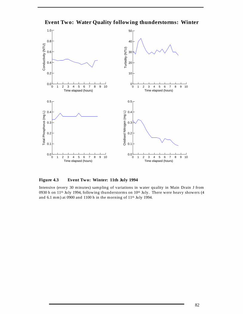
82
Event Two: Water Quality following thunderstorms: Winter
0 1 2 3 4 5 6 7 8 9 10Time elapsed (hours)
0.0
0.2
0.4
0.6
0.8
1.0
Con
duct
ivity
(N
TU
)
0 1 2 3 4 5 6 7 8 9 10Time elapsed (hours)
0
10
20
30
40
50
Tur
bidi
ty (
NT
U)
0 1 2 3 4 5 6 7 8 9 10Time elapsed (hours)
0.0
0.1
0.2
0.3
0.4
0.5
Tot
al P
hosp
horu
s (m
g L)
0 1 2 3 4 5 6 7 8 9 10Time elapsed (hours)
0.0
0.1
0.2
0.3
0.4
0.5
Oxi
dise
d N
itrog
en (
mg
L)
Figure 4.3 Event Two: Winter: 11th July 1994
Intensive (every 30 minutes) sampling of variations in water quality in Main Drain J from0930 h on 11th July 1994, following thunderstorms on 10th July. There were heavy showers (4and 6.1 mm) at 0900 and 1100 h in the morning of 11th July 1994.

83
Event Three: Water Quality: 17-18 May 1995
0 3 6 9 12 15 18 21 24Elapsed Time (hours)
0.0
0.2
0.4
0.6
0.8
1.0
Con
duct
ivity
0 3 6 9 12 15 18 21 24Elapsed Time (hours)
0
50
100
150
200
250
300
Tur
bidi
ty (
NT
U)
0 3 6 9 12 15 18 21 24Elapsed Time (hours)
0.0
0.2
0.4
0.6
0.8
1.0
Tot
al P
hosp
horu
s (m
g L)
0 3 6 9 12 15 18 21 24Elapsed Time (hours)
0
1
2
3
4
Org
anic
Nitr
ogen
(m
g L)
0 3 6 9 12 15 18 21 24Elapsed Time (hours)
0
1
2
3
4
Oxi
dise
d N
itrog
en (
mg
L)
Figure 4.4 Event Three: Water Quality: 17-18 May 1995
Variations in water quality in Main Drain J over 21 hours from 1110 h to 0830 h for selectedparameters.

84
Chapter 5Chapter 5
Trunks and Trunks and Tribs Study: Main Drain JTribs Study: Main Drain J
5.15.1 Water quality in exit drainsWater quality in exit drains
MonitoringMonitoringThe water quality of large drains leaving irrigation areas is monitored routinely bygovernment agencies industry corporations, and the results are published in reports(eg Buchan 1994, Shepheard 1994), rather than in scientific journals. In general,interpretation of temporal trends in monitoring data is limited, and the significanceof different hydrological conditions rarely explored. The Trunks and Tribs study(Chapter 3) monitored water quality under low-flow conditions in lateral drains, andshowed the significance of land use as a factor determining nutrient concentrations.In that study, the laterals were treated as a population of separate drains, and theircontribution to Main Drain J was not explored. The aim was to identify nutrient‘hot-spots’. Approaches based on modelling (eg Allanson et al. 1993) were notfeasible because nutrient yield data, which is the data needed for modelling nutrientfluxes into irrigation drains, is generally not available.
The two themes addressed here are an evaluation of Main Drain J as a source or asink for nutrients (as per project brief, Appendix A), and an estimate of nutrientyields from sub-catchments within an irrigation area. Water quality within the mainexit drain, Main Drain J, is also described.
Within-drain processesWithin-drain processesTheoretically, through nutrient transformations, water quality can change withoutchanging total load. Total nutrient load can decrease by deposition of particulateforms or by loss of gaseous forms; it can increase (other than by tributary input)only by entrainment and scouring.
Changes in load can therefore be expected at any time of the year. The sustainedhigh flows likely to cause entrainment of sediment and particulate forms ofphosphorus and nitrogen occur mainly during the irrigation season (Figure 5.1).The months most likely to have extreme rainfall at Griffith (Table 5.1) also occurduring the irrigation season. High rainfall results in rapid increase in drainagedischarge (see Figure 1.4, and Chapter 4), sometimes with high velocities. Forexample, the highest velocity measured by DWR hydrographers while ratingYoogali gauge was 0.85 m s-1 and this was at a time of peak discharge (1249 ML d-1)during an exceptional rain event in April 1989 (Figure 5.1). Conversely, the low-flow condition suitable for deposition, whether by settling or by flocculationresulting from saline in-flows, occur mainly but not exclusively outside the irrigationseason.
The redox and oxic status of drain sediments has not been surveyed but the anoxicsediments needed for de-nitrification are more likely to occur under low flowconditions. The rationale for this is that de-nitrification requires a carbon source,and it is only under low flow conditions, particularly after a high flow pulse, that

85
organic material is likely to be deposited on the sediments. Because of thesediffering conditions, drains, like other wetland systems, probably alternate betweenbeing a source and sink for nutrients (cf Harris 1996, Raisin et al. 1997).
Nutrient yield from sub-catchmentsNutrient yield from sub-catchmentsThe nutrient modelling for the Murray-Darling Basin main rivers (GHD 1992) musthave made certain assumptions regarding nutrient export coefficients, possiblyrelying on studies from North America. A recent review of nutrient export ratesfound that Australian studies “do not total many more than 20” (Young et al. 1996),and of these, about half were on urban catchments. Australian data were availablefor land uses such as urban, improved pasture, unimproved pasture, cropping,market gardens and forests (Young et al. 1996), but no yields specific to irrigatedagriculture were given. A few Australian yield data have been reported recently (egGBWQWG 1995).
Defining nutrient yields for “irrigation” as a land use is an oversimplification,because irrigation areas are not internally homogeneous. The diversity of cropsgrown, as well as differences in cultivation and management history, soils andclimate, suggest that yield data, even for the same crops, can be expected to varybetween regions. The Trunks and Tribs study was an opportunity to estimatenutrient generation rates under low-flow conditions, uninfluenced by rainfall.
ObjectivesObjectivesAn assessment of Main Drain J as either nutrient source or sink was made byextending the Trunks and Tribs study on lateral drains (Chapter 3). The addition ofthree sites within Main Drain J made it possible to compare an expected load(determined as the sum of tributary drains) with a measured load (actual load in thedrain), and make inferences regarding sources and sinks. Direct measurements oferosion, de-nitrification, bank retreat and benthic metabolism were not feasiblewithin resources available. Specific objectives were:
♦ To describe temporal patterns in water quality in Main Drain J
♦ To determine if any nutrient gains or losses were occurring in an exit drain
♦ To estimate nutrient yields from catchments with different land uses.
5.25.2 MethodsMethods This is part of the Trunks and Tribs study, so the context is the Mirrool IrrigationArea in the MIA. Site selection, sampling procedures and chemical analyses weredescribed previously (Chapter 3.2).
Field sites There were three sites in Main Drain J: Site T (Top) was the mostupstream site, near Yenda; Site Y (Yoogali) was close to Yoogali gauge; Site B(Bottom) was downstream of all other sites (Figure 3.1). The catchment area forthese is given in Table 3.1). Note that Site T is an arbitrary reference point forexploring types of changes, and is itself a drain from BR-100 catchment (Table 3.1).
Sampling At each site, discharge was measured using a flow-meter, and a 500mL water samples was collected for EC, SS, TP, TN, TKN and NOx as describedabove (chapter 3.2 and Appendix D). Sampling frequency, storage and processing

86
was the same as for the tributary drain study and samples were collected at thesame time.
Within-drain processesWithin-drain processes The measured load was the product of discharge and concentration, and wascalculated for each month, for each of five water quality parameters: SS, TP, andorganic and oxidised forms of nitrogen.
The expected load was the sum of all the inputs from the upstream tributary loads(as determined in the first part of the Trunks and Tribs Study) for a given date. Tocompensate for the small inputs not monitored during the earlier study, a correctionfactor was used, based on discharge, and was calculated separately for Site Y andSite B. The correction factor was (sum of all tributary discharge) / (discharge at SiteB or Y) and most adjustments were small, being within 10%. The largest adjustmentwas made in June 1995 (by a factor of 0.58) and the smallest was in October (0.998).June data are not included in interpretation.
The evidence for in-stream processes was based on a comparison of measuredversus observed nutrient loads. The difference between these was expressed inrelative terms as a dimensionless ratio: (Measured-Expected)/(Measured). Valuesless than 0.10 (ie within 10%) were considered as within the bounds of error, andtherefore of not showing change. Values greater than 0.10, ie when measured loadexceeded estimated load by more than 0.10 indicated a gain down Main Drain J, andvalues less then -0.10 indicated a loss (the drain as a sink).
Nutrient yieldsNutrient yields Nutrient yields from sub-catchments were estimated for 21 of the 24 sub-catchmentsmonitored during the Trunks and Tribs study (Chapter 3), thus are for low-flowconditions only. Yields were calculated for SS, TP, TN, TKN and NOx. The threesub-catchments which were not included were: Site 3 (McKissack Road) which wasprobably being used as a supply system so had an a-typical discharge for its landuse, Site 2, which was thought to have a significant urban input and Site 20, whichwas particularly large (8038 ha, see Table 3.1) and diverse, and had an urban inputfrom eastern and newer areas of Griffith.
Yield was for each irrigation drain was the sum of each monthly load, from Octoberto April, divided by catchment area; units are kg ha-1 per irrigation season. Themonthly load for each nutrient was the instantaneous load (concentration as mg L-1
x discharge as L s-1) extrapolated to a daily load (kg d-1) then to a monthly load(tonnes month-1). This makes a conservative assumption that the low-flowconditions when sampling prevailed throughout the month, ie there were no rainevents. Nutrient export for each catchment (kg ha-1) during the irrigation seasonwas the total load exported from October to April inclusive expressed on an arealbasis.
The effect of irrigation on nutrient export was determined by comparing export ratesduring the seven months of the irrigation season with the export rates duringautumn (May-June). The comparison was a mean monthly export for each timeperiod, expressed as a ratio, tested for significance by one-way ANOVA.
Three land uses were recognised here: rice, grapevines and trees, referring to citrusand stone fruit, designated R, G and T. These were initially perceived as being toosimplistic, so were broken down into more realistic combinations: R and G, G and
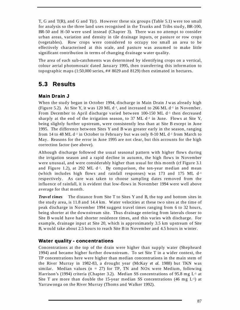
87
T, G and T(R), and G and T(r). However these six groups (Table 5.1) were too smallfor analysis so the three land uses recognised in the Trunks and Tribs study, BR-100,BR-50 and H-50 were used instead (Chapter 3). There was no attempt to considerurban areas, variation and density in tile drainage inputs, or pasture or row crops(vegetables). Row crops were considered to occupy too small an area to beeffectively characterised at this scale, and pasture was assumed to make littlesignificant contribution in terms of changing drainage water quality.
The area of each sub-catchments was determined by identifying crops on a vertical,colour aerial photomosaic dated January 1995, then transferring this information totopographic maps (1:50,000 series, ## 8029 and 8129) then estimated in hectares.
5.35.3 ResultsResults
Main Drain JMain Drain J When the study began in October 1994, discharge in Main Drain J was already high(Figure 5.2). At Site Y, it was 120 ML d-1, and increased to 266 ML d-1 in November.From December to April discharge varied between 100-150 ML d-1 then decreasedsharply at the end of the irrigation season, to 37 ML d-1 in June. Flows at Site Y,being slightly further upstream, were consistently less than at Site B except in June1995. The difference between Sites Y and B was greater early in the season, rangingfrom 14 to 48 ML d-1 in October to February but was only 8-10 ML d-1 from March toMay. Reasons for the error in June 1995 are not clear, but this accounts for the highcorrection factor (see above).
Although discharge followed the usual seasonal pattern with higher flows duringthe irrigation season and a rapid decline in autumn, the high flows in Novemberwere unusual, and were considerably higher than usual for this month (cf Figure 3.1and Figure 1.2), at 292 ML d-1. By comparison, the ten-year median and mean(which includes high flows and rainfall responses) was 173 and 175 ML d-1
respectively. As care was taken to choose sampling dates removed from theinfluence of rainfall, it is evident that low-flows in November 1994 were well aboveaverage for that month.
Travel times The distance from Site T to Sites Y and B, the top and bottom sites inthe study area, is 11.8 and 14.4 km. Water velocities at these two sites at the time ofpeak discharge in November 1994 suggest travel times ranging from 6 to 32 hours,being shorter at the downstream site. Thus drainage entering from laterals closer toSite B would have had shorter residence times, and this varies with discharge. Forexample, drainage input at Site 20, which is approximately 3.5 km upstream of SiteB, would take about 2.5 hours to reach Site B in November and 4.5 hours in winter.
Water quality - concentrationsWater quality - concentrations Concentrations at the top of the drain were higher than supply water (Shepheard1994) and became higher further downstream. To set Site T in a wider context, theTP concentrations here were higher than median concentrations in the main stem ofthe River Murray in 1982-83, a drought year (McKay et al. 1988) but TKN wassimilar. Median values (n = 27) for TP, TN and NOx were Medium, followingHarrison’s (1994) criteria (Chapter 3.2). Median SS concentrations of 95.8 mg L-1 atSite T are more than double the 15-year median SS concentrations (46 mg L-1) atYarrawonga on the River Murray (Thoms and Walker 1992).

88
EC, SS, TP and TN show different trends through time (Figure 5.3), and these aresimilar to the seasonal trends shown in the lateral drains (Figure 3.3). Thelongitudinal changes between top and bottom of the study area fall into certainphases.
Three phases were evident with EC. In the first phase, from October to February,EC was relatively low at the top of Main Drain J, being consistently less than 200 µScm-1 at Site T. But by Site Y near Yoogali, 11.75 km downstream and 20 drain inputsfurther on, EC had doubled and was consistently more than 400 µS cm-1. Thisshowed a major contribution from lateral drains during the spring-summer months.In the second phase, the difference between Site T and Sites Y and B graduallydiminished, suggesting that the contribution from the lateral drains was decreasingin February to April. By April EC at these three sites was 154, 264 and 215 µS cm-1
respectively. In May and June, the third phase, EC at all three sites increased 3-4fold, suggesting that concentrations in lateral drains and the head of Main Drain Jwere quite similar.
Longitudinal changes in concentrations of SS also showed three phases, but withdifferent timings. For the first three months, from October to December,concentrations of SS were consistently low at Site T, <30 mg L-1, but increased downthe drain and at Sites Y and B they were 2-3 times higher, ranging from 58-87 mg L-1.This showed a major contribution from inflowing drains. In the second phase,December to March, SS concentrations rose at all sites and peaked in February. SSwas particularly high at Site T, over 335 mg L-1, which was a 10-fold increase onspring levels. At Sites Y and B the February peak was lower, 209 and 194 mg L-1,and represented only a 2-3 fold increase. These SS concentrations are very high:concentrations of 200+ mg L-1 are typical of the Murrumbidgee during floods (egOlive et al. 1996). The source of this SS was not determined but could be accountedfor by cultivation, building, or channel-forming activities. The increase in SS wasgenerally lower at the downstream sites, indicating an overall dilution or lossprocess in later summer (Figure 5.3). In the third phase, from March onwards, thedifference between upstream and downstream sites remained stable, making thisphase similar to the first one.
There were no clear phases with TP concentrations. These generally increasedbetween Site T and the two bottom sites but not in a coherent way. In spring,October and November, downstream concentrations of TP were 4-7 times higherthan upstream (66-280 compared with 39-42 µg L-1), suggesting a major inflow of TPbetween Site T and Sites Y and B. Concentrations of TP rose at Site T after Decemberand peaked in February and March at 126 and 140 µg L-1 coincident with theincrease in SS. Such increases were not evident at the downstream sites (Figure 5.3).
Like EC and SS, TN also had three phases. Initially, from October to December, TNincreased several hundred-fold down Main Drain J, from 42-81 µg L-1 at Site T to1950-2940 µg L-1 at Sites Y and B. This pointed to an enormous contribution fromlateral drains with no evidence of dilution effect. In the second phase, fromDecember, TN concentrations at the top of Main Drain J rose reaching a peak of1280-1290 µg L-1 in January-February, then declining. This peak was not evident atthe downstream sites where TN concentrations decreased steadily, falling to 930 and840 µg L-1 at Sites Y and B in April. Nitrogen inputs from lateral drains betweenSites T, and Y and B increased enormously in autumn, the third phase.
The forms of nitrogen had distinctive trends (not shown). At Site T, NOx wasconsistently below detection limits so TN was almost entirely organic. However, at

89
the two lower sites, NOx was consistently 30-49% of TN, except in December andagain April when it rose to 52-67% and 61-72% at Sites Y and B respectively.
Water quality loadsWater quality loads The low-flow loads of SS, TP, TKN and NOx did not show the same temporal trendsas discharge (Figure 5.4).
SS load increased rapidly at the beginning of the irrigation season and peaked atSites Y and B in February at 277 and 306 g s-1, equivalent to 670 and 740 tonnesmonth-1. This was coincident with high SS concentrations (Figure 5.3). Loads of TPwere highest at the beginning of the irrigation season, and lowest in May and June,outside the irrigation season. The high load at Site B in November, of 0.762 g s-1
equivalent to 1.97 tonnes month-1, was due to the combined effect of high dischargeand high TP concentrations. The highly variable TP concentrations at Sites Y and Bresulted in TP loads at the upstream site (Site Y) appearing to exceed loads at thedownstream site (Site B) on 4/9 occasions. Reasons for these apparently anomalousresults are not clear but could be due to adsorption and bioturbation (Meredith,pers. obs. 1996).
Loads for organic and NOx both peaked at both Sites Y and B in November, at loadsequivalent to 13.9 and 12.1 tonnes month-1 (for TKN) and 9.6 and 10.5 tonnes month-
1 (for NOx). Nitrogen loads were also high in January and in May. NOx loadsfollowed discharge, being highest in November, and were consistently higher at SiteB than Site Y.
The loads of suspended sediment exported down Main Drain in low-flows showedthree interesting characteristics. First was the quantity, which was measured intonnes and exceeded the other nutrient loads by several orders of magnitude (Table5.2). At Site B, for example, the total SS load during the irrigation season was 3227tonnes compared with an estimated 9.68 tonnes of TP and 74 tonnes of TN for thesame period. Second was the timing of that export, and its link with the irrigationseason. For example, the ratio of mean monthly loads for Sites B and Y for two timeperiods shows that SS export was 700-fold higher during the irrigation season.Third is the composition of the suspended sediment load. Even if all the TP and allthe TN present were particulate and organic, these nutrients would only comprise atthe most only 0.3% and 2.2% of sediment load, suggesting that most of SS isinorganic.
Within-drain processesWithin-drain processes Load changes within Main Drain J greater than 0.10 or less than –0.10 were hereconsidered as indicative of net gain or net loss (source or sink). An unresolved errorin discharge data for June (Figure 5.2) makes load calculations for this monthunreliable, and June data are not considered in the analyses below, although shownon the diagrams.
Changes in SS load (Figure 5.5) were positive and greater than 0.10, so assumed tobe significant, at both downstream sites in the first part of the irrigation season(October, November, December) and then again in February, indicating a gain atthese times. The evidence for sediment deposition was limited to one site, Site Y, ontwo occasions, January and May.
There was little consistency between SS and TP loads. At both downstream sites, TPload was higher than expected only in October. Otherwise there was little difference

90
between expected and measured TP loads, with no difference in four out of ninemonths (December, February, March and April).
Oxidised and organic nitrogen showed different and almost complementary trends.Loads of TKN were larger than expected at both sites in October, December andMay, but with no change in January and March, and no consistent evidence of loss.Loads of NOx were higher than expected in November, February and April, andshowed no net change in October, December and January. In-stream increases inTKN load in October could be caused by entrainment resulting from the increasingflows. Gains in NOx loads could be attributed to nitrification, or could reflect thevariable nature of NOx concentrations (figure 4.2, Event One), although the locationof Site B, downstream of a large bridge with much turbulence was expected toremove such patchiness.
Nutrient yieldsNutrient yields Yield for SS ranged widely from 140 in BR-100 sub-catchments to 259 kg ha-1 fromBR-50 catchments (Table 5.3). Differences between land use types were notsignificant. TP yield of 0.82 and 0.85 kg ha-1 for H-50 and BR-50 was nearly twice asmuch as from BR-100 sub-catchments (p = 0.08). The yield of TKN was very similaracross the three land uses, ranging from 2.39 to 3.1 kg ha-1, with no significantdifference. In contrast, NOx and consequently also TN showed a wide range (Table5.3), with BR-100 having the lowest yields and H-50 the highest. For NOx and TN,differences between types of land use were significant (p = 0.03, and p = 0.03respectively).
5.45.4 DiscussionDiscussion This analysis of nutrient sources and sinks in Main Drain J used a coarse applicationof mass balance to determine if changes were occurring. Comparative data arelacking as studies of benthic metabolism and sedimentary processes are rare instreams and rivers in Australia and, as far as can be determined, have not beenattempted in irrigation drains. This was an exploratory analysis, and the findingsshould be considered indicative rather than definitive.
Nonetheless, despite the coarseness of the technique, the findings were consistentwith field observations of conditions in Main Drain J. For example, in October therewere gains in loads of suspended sediment, TP and TKN, suggesting entrainment ofparticulate forms. October was also the time of rapidly increasing discharge whichis consistent with this.
The dominant load change detected was gain rather than loss. Overall, there waslittle evidence of in-transit losses. Deposition, as indicated by a relative change of –0.1, occurred rarely and only for SS and TP at Site Y. Again, this was consistent withfield measurements. Velocity was slower at Site Y (Figure 5.1), and cross-sectionalarea (not shown) was wider than at Site B. Being wider and more slow-moving, SiteY was therefore more suitable as a foraging habitat for carp. Thus bioturbationshould be considered a possible mechanism to explain the increase in SS load whichoccurred only at this site, in April (Figure 5.5).
Changes in the load of NOx did not directly responding to velocity-driven processesof deposition and entrainment. Thus the increased loads that occurred in threemonths at both sites (November, February and April) suggest nitrification wasoccurring. This is a tentative conclusion which needs to be supported by benthic

91
metabolism studies. It assumes neither oxygen nor ammonium were limiting. Thehigh discharge suggests turbulence so this may be a reasonable assumption foroxygen, but there is no evidence of the organic load reducing as ammoniumconcentrations were consistently below detection limits.
The nutrient yields reported here refer only to part of the year (seven months withinthe irrigation season, from October to April) and are for low-flow conditions,unaffected by rainfall. They do not include the very beginning of the irrigationseason, a time when discharge steadily increases, and do not account for other rapidincreases such as storm events or rejection flows (see Chapter 4). Extrapolatingthese to the whole year would give a biased estimate, as shown by the very bigdifferences in monthly export during the irrigation season and outside it (Table 5.3).
All the phosphorus and nitrogen yields estimated for Mirrool Irrigation Area werelow for all sub-catchments. Row crops in North America, for example, have amedian annual nutrient export of 2.3 kg ha-1 y-1 for phosphorus and 8.5 kg ha-1 y-1
for nitrogen (Young et al. 1996). In northern Victoria, Australia, perennial pasture isthe dominant crop and export coefficients have been estimated as 5.24 and 13.1 kgha-1 TP and TN during the irrigation season and 0.30 TP and 0.8 TN kg ha-1 outsidethe irrigation season (GBWQWG 1995). High nutrient losses in this Victorian study,as elsewhere (eg Neeson 1996), were attributed to high losses of fertiliser in run-off.
Conclusions and findingsConclusions and findings♦ Correct diagnosis of the water quality problem is essential. Suspended
sediment, rather than nitrogen and phosphorus, was the main nutrient exportfrom this irrigation area. Even under low-flows, large quantities of suspendedsediment were exported during the warmer months: and SS yield rates werehigh.
♦ Nutrient yield rates were not high when compared with values reported in theliterature.
Reasons for these high SS exports were not determined but must be a consequenceof activities in sub-catchments within the irrigation area. Water managers shouldconsider restricting this aspect of pollution, as it could represent a future cost in de-silting activities.
♦ The main exit drain in Mirrool IA was a periodic source of nutrients, noticeablySS, TP and possibly NOx, between October and June. This was only partlyattributable to increases in discharge. The drain rarely functioned as a nutrientsink, except possibly at one site, and for site-specific reasons.
ReferencesReferences
Allanson, P., Moxey, A. and White, B. (1993). Agricultural nitrate emission patterns in theTyne catchment. Journal of Environmental Management 38:219-232.
Buchan, A. (1994). Coleambally Irrigation Area: Surface Water Quality data report. TechnicalServices Report 94/10. Department of Water Resources, Murrumbidgee region,February 1994.
GBWQWG (1995). Nutrients in irrigation drainage water from the Goulburn and Brokencatchments: Issues paper. Number 5. Goulburn Murray Water, Tatura.
92
GHD (1992). An investigation of nutrient pollution in the Murray-Darling River system. Reportprepared by Gutteridge, Haskins and Davey, for the Murray-Darling BasinCommission.
Harris, G. (1996). Catchments and aquatic ecosystems: nutrient ratios, flow regulation ecosystemimpacts in rivers like the Hawkesbury-Nepean. CRC Freshwater Ecology DiscussionPaper. June 1996.
Harrison, J. (1994). Review of nutrients in irrigation drainage in the Murray-Darling Basin.CSIRO Division of Water Resources. Seeking Solutions. Water Resources Series:No 11.
McKay, N. Hillman,T. and Rolls, J. (1988). Water quality of the River Murray: Review ofmonitoring, 1978 to 1986. Murray-Darling Basin Commission, Canberra.
Neeson, R. (1996). The fate of nutrients - literally $$’s down the drain. Farmer’s Newsletter178:11-13.
Olive, L.J., Olley, J.M., Wallbrink, P.J.and Murray, A.S. (1996). Downstream patterns ofsediment transport during floods in the Murrumbidgee River, NSW, Australia. Z.Geomorph. N.F. Suppl. Bd. 105:129-140.
Raisin, G.W., Mitchell, D.S. and Croome, R.L. (1997). The effectiveness of a smallconstructed wetland in ameliorating diffuse nutrient loadings from an Australianrural catchment. Ecological Engineering 9:19-35.
Shepheard, M. (1994). Murrumbidgee Irrigation Area: Surface Water Quality project, 1993.Technical Services Report No. 94/07. NSW Department of Water Resources,Murrumbidgee region.
Thoms, M.C. and Walker, K.F. (1992). Sediment transport in a regulated semi-arid river: theRiver Murray, Australia. In: R.D.Robarts and M.L. Bothwell (eds). Aquaticecosystems in semi-arid regions: implications for resource management. NHRISymposium Series 7, Environment Canada, Saskatoon, Canada.
Young, W.J., Marston, F.M. and Davis, J.R. (1996). Nutrient exports and land use inAustralian catchments. J. Environmental Management 47:165-183.
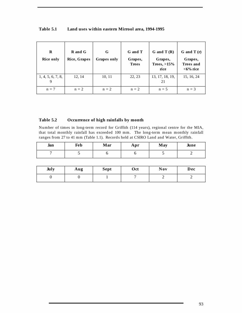
93
Table 5.1 Land uses within eastern Mirrool area, 1994-1995
R
Rice only
R and G
Rice, Grapes
G
Grapes only
G and T
Grapes,Trees
G and T (R)
Grapes,Trees, >15%
rice
G and T (r)
Grapes,Trees and<6% rice
1, 4, 5, 6, 7, 8,9
12, 14 10, 11 22, 23 13, 17, 18, 19,21
15, 16, 24
n = 7 n = 2 n = 2 n = 2 n = 5 n = 3
Table 5.2 Occurrence of high rainfalls by month
Number of times in long-term record for Griffith (114 years), regional centre for the MIA,that total monthly rainfall has exceeded 100 mm. The long-term mean monthly rainfallranges from 27 to 41 mm (Table 1.1). Records held at CSIRO Land and Water, Griffith.
Jan Feb Mar Apr May June
7 5 6 6 5 2
July Aug Sept Oct Nov Dec
0 0 1 7 2 2

94
Table 5.3 Loads and seasonal comparisons in Main Drain J
Nutrient loads at three sites down Main Drain J for two time periods, October to Aprilinclusive (the main irrigation season), and May-June (autumn). Ratio is the ratio of meanmonthly load during the seven months of the irrigation season to the two months of autumn.n.d means no data.
TotalOctober-
April
TotalMay-June
Monthlymean,
October-April (n=8)
Monthlymean,
May-June(n=2)
Ratio
SUSPENDED SEDIMENTS (tonnes)
Site TSite YSite B
6629243227
dry1.01.1
8.3365.5403.4
dry0.510.53
717764
TOTAL PHOSPHORUS (tonnes)
Site TSite YSite B
0.058.409.68
dry0.240.22
0.0061.0501.209
dry0.1220.111
8.610.7
ORGANIC NITROGEN (tonnes)
Site TSite YSite B
0.6839.0540.42
dry5.026.03
0.084.885.05
dry2.513.01
1.941.68
OXIDISED NITROGEN (tonnes)
Site TSite YSite B
n.d.28.2634.10
dry4.615.20
3.544.26
dry2.302.60
1.531.64
TOTAL NITROGEN (tonnes)
Site TSite YSite B
0.6867.3374.53
dry9.63
11.23
0.088.429.32
dry4.815.61
1.751.66

95
Table 5.4 Nutrient yields
Mean nutrient yield (with SE) for each land use based on 21 sub-catchments. Yield units arekg ha-1 and refer to low-flow, rainfall-unaffected conditions during the irrigation season,based on data for October to April.
Above: land uses identified as combinations of G, R and T (see text).
Below: land uses identified as in Chapter 3.
LAND USE SS TP Organic N Oxidised N Total N
G(n=2)
286.6(15.75)
1.18(0.40)
3.530.34)
0.15(0.15)
3.68(0.19)
GT(n=2)
188.5(138.5)
0.94(0.31)
3.43(0.63)
9.84(9.27)
13.26(9.91)
GT(R)(n=3)
154.6(60.3)
0.46(0.22)
2.04(0.78)
3.23(1.65)
5.27(2.01)
GTR(n=5)
282.2(67.13)
0.95(0.09)
3.01(0.54)
6.09(4.01)
9.1(4.28)
R(n=7)
140.4(46.73)
0.42(0.13)
2.39(0.26)
0.10(0.07)
2.49(0.28)
RG(n=2)
230.5(102.54)
0.78(0.26)
4.16(0.87)
0.24(0.01)
4,40(0.88)
LAND USE SS TP Organic N Oxidised N Total N
BR-100(n=7)
140.4(46.73)
0.42(0.13)
2.39(0.26)
0.10(0.07)
2.49(0.28)
BR-50(n=9)
258.5(45.55)
0.85(0.14)
3.1(0.43)
1.75(0.98)
4.85(0.98)
H-50(n=6)
193.4(40.20)
0.82(0.12)
2.98(0.43)
8.35(3.80)
11.34(4.13)
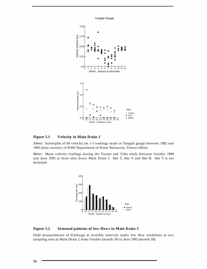
96
Yoogali Gauge
0 1 2 3 4 5 6 7 8 9 10 11 12
Month: January to December
0.0
0.25
0.50
0.75
1.00
Vel
ocity
(m
etre
s se
c)
9 10 11 12 13 14 15 16 17 18 19Month: October to June
0.0
0.5
1.0
1.5
Vel
ocity
(m
etre
s se
c)
BottomTopYoogali
Sites
Figure 5.1 Velocity in Main Drain J
Above: Scatterplot of 64 velocity (m s-1) readings made at Yoogali gauge between 1982 and1993 (data courtesy of NSW Department of Water Resources, Tumut office).
Below: Mean velocity readings during the Trunks and Tribs study between October 1994and June 1995 at three sites down Main Drain J: Site T, Site Y and Site B. Site T is notincluded.
9 10 11 12 13 14 15 16 17 18 19Month: October to June
0
100
200
300
400
Dis
char
ge (
ML
day)
Site YSite B
Sites
Figure 5.2 Seasonal patterns of low-flows in Main Drain J
Field measurements of discharge at monthly intervals under low flow conditions at twosampling sites in Main Drain J, from October (month 10) to June 1995 (month 18).

97
Conductivity
8 9 10 11 12 13 14 15 16 17 18 19Month: October to June
0
200
400
600
800
1000
1200
Con
duct
ivity
(m
icro
S c
m)
Suspended Sediments
8 9 10 11 12 13 14 15 16 17 18 19Month: October to June
0
100
200
300
400
SS
(m
g L)
Total Nitrogen
8 9 10 11 12 13 14 15 16 17 18 19Month: October to June
0
1000
2000
3000
4000
5000
TN
(m
icro
g L)
Total Phosphorus
8 9 10 11 12 13 14 15 16 17 18 19Month: October to June
0
100
200
300T
P (
mic
rog
L)
Figure 5.3 Water quality changes in Main Drain J
Longitudinal (Top, Yoogali and Bottom) and seasonal (October 1994 to June 1995) changes inmean EC, SS, TP and TN. Solid line is Site T (Top), dotted line is Site Y (Yoogali) and dashedline is Site B (Bottom).

98
9 10 11 12 13 14 15 16 17 18 19Month: October to June
0
100
200
300
400
SS
load
(g
sec)
9 10 11 12 13 14 15 16 17 18 19
Month: October to June
0
200
400
600
800
TP
load
(m
g se
c)
Site YSite B
Sites
9 10 11 12 13 14 15 16 17 18 19Month: October to June
0
2
4
6
8
10
TK
N l
oad
(g s
ec)
9 10 11 12 13 14 15 16 17 18 19
Month: October to June
0
1
2
3
4
5
NO
x lo
ad (
g se
c)
Site YSite B
Sites
Figure 5.4 Seasonal loads in Main Drain J
Nutrient loads in Main Drain J under low flow conditions only, from October 1994 to June1995, as measured at Site Y near Yoogali gauge and Site B, just downstream of OldWilbriggie Road.

99
Suspended Sediment
9 10 11 12 13 14 15 16 17 18Month in year: October to June
-0.5
0.0
0.5
1.0
Rel
ativ
e C
hang
e
Yoogali gaugeBottom
Site on MDJ
Total Phosphorus
9 10 11 12 13 14 15 16 17 18Month in year: October to June
-0.5
0.0
0.5
1.0
Rel
ativ
e C
hang
e
Yoogali gaugeBottom
Site on MDJ
Organic Nitrogen
9 10 11 12 13 14 15 16 17 18Month in year: October to June
-1.0
-0.5
0.0
0.5
Rel
ativ
e C
hang
e
Yoogali gaugeBottom
Site on MDJ
Oxidised Nitrogen
9 10 11 12 13 14 15 16 17 18Month in year: October to June
-2
-1
0
1
Rel
ativ
e C
hang
e
Yoogali gaugeBottom
Site on MDJ
Figure 5.5 Load changes within Main Drain J
Ratio of measured to expected load, with expected being sum of upstream tributaries (seetext) with a correction factor applied, based on discharge for Site Y near Yoogali gauge andSite B, on Main Drain J.

100
G GTGT(R
)GTR R RG
Catchments in Mirrool
-100
0
100
200
300
400
500
SS
yie
ld (
kg h
a-1)
G GTGT(R
)GTR R RG
Mirrool catchments
0.0
0.5
1.0
1.5
2.0
2.5
TP
yie
ld (
kg h
a-1)
G GTGT(R
)GTR R RG
Mirrool catchments
-10
0
10
20
30
NO
x yi
eld
(kg
ha-1
)
G GTGT(R
)GTR R RG
Mirrool catchments
-10
0
10
20
30
40
50
TN
yie
ld (
kg h
a-1)
G GTGT(R
)GTR R RG
Mirrool catchments
0.0
2.5
5.0
7.5
TK
N y
ield
(kg
ha-
1)
Figure 5.6 Nutrient yields by land use
Mean (with SE) for the main land use groupings in the Mirrool Study area. Nutrient yieldsare as kg per hectare, and relate to data collected in the irrigation season, only (October toApril). Sample sizes for G, GT and RG are small (see text), with n = 2 (Table 5.2).

101
Chapter 6Chapter 6
Sediments and Sediments and BioturbationBioturbation
6.16.1 Sediments and Sediments and bioturbationbioturbationFor rooted macrophytes, sediments provide both rooting substrate and nutrientsource. The extent to which aquatic macrophytes utilise nutrients from thesediments, rather than from the water column, depends partly on life form, partlyon species, and partly on the relative richness of nutrients in the sediment versus thewater column. Sediments can be resuspended into the water column, a processknown as bioturbation if the process is biological. Examples of organismsimplicated in bioturbation are tubificids, polychaetes, a marine worm (eg Clavero etal. 1994), and benthivorous fish, in lakes and wetlands (eg Breukelaar et al. 1994).Bioturbation can be an important pathway for transferring nutrients from thesediment to the water column.
In rivers and streams, unconsolidated benthic sediments originate from channelbanks or are delivered as suspended sediments from upstream, so may originatefrom anywhere further up the catchment. In irrigation drains, likely sources areerosion and scouring of channel walls, surface erosion from irrigated land, ortransported in through supply water. Nutrient status is determined partly by theirlithology, and partly by absorption-desorption processes whilst in transit or afterbeing deposited. This thus includes fertilisers applied to crops in the catchment andcarried to the drain via run-off or percolation, as well as domestic and industrialwastes, although these are not so well-recognised. Sediments in irrigation drainshave been little investigated in Australia. Evidence that there are high sedimentloads in irrigation returns to rivers (eg McKay et al. 1988, Thoms and Walker 1992)makes them, and their source, an important water and river management issue.
The extent to which suspended sediments are transported through and out of anirrigation area or deposited within it – even temporarily – is determined by flow.The large annual range in discharge and velocity (Figures 1.2, 1.3, 3.2, 5.1 and 5.2) indrains through the irrigation cycle and in the concentrations and loads of suspendedsediments has been described previously (storm events and seasonal patterns inChapters 3, 4 and 5). Because of this, the depth and extent of unconsolidatedsediments will be variable and, as in rivers, their composition influenced byupstream factors, namely land use and discharge.
Bioturbation and CarpBioturbation and CarpCarp Cyprinus carpio L. are an introduced fish which are abundant in manyirrigation areas. Adult fish typically feed by foraging for invertebrates and otherfood items in the benthos (ie the bottom muds) of wetlands and lakes, and do this bysucking in and expelling water and mud (Sibbing 1991) as shown below (Figure 6.1).This disturbs the sediment, resuspending it into the water column, a processreferred to as bioturbation. This increases turbidity and, regardless of whether thisis a temporary or a sustained effect, this affects water quality. In turn, this hascertain ecosystem consequences (eg Roberts et al. 1995, Roberts and McCorkelle1995), particularly in enclosed water bodies such as wetlands and lakes. Carp are

102
abundant in most Australian inland irrigation areas (Meredith 1996, Jackel 1996)making it likely that bioturbation is a significant factor affecting the quality ofdrainage water, and in particular phosphorus. As total phosphorus concentrationsin sediment tend to be much higher than in the overlying water, feeding carp couldpotentially increase phosphorus in the water column.
There has been considerable concern in the water industry (Jackel 1996) that carphave an adverse effect on irrigation drains, degrading water quality and threateningbank stability and hence also irrigation structures. Assessing the overall significanceof carp for the irrigation industry is outside the scope of this study, but presents amajor scientific challenge. Some initial studies on carp biology and impact havebeen done (Adamek 1998, Roberts and McCorkelle 1995) but firm progress isdifficult because of the lack of scientific studies on drain ecology in Australia.
ObjectivesObjectivesThe objectives were to evaluate the role of carp in degrading the quality of drainagewater, by considering drain sediments, bioturbation and carp within an irrigationarea. This part of the project addressed the significance of bioturbation, as perproject brief (Appendix A). By including sediment, these findings were expected tocontribute to the overall objective of evaluating the feasibility of drains as a habitatfor macrophytes.
The research on carp was a study on bioturbation and sediments, done by ShaunMeredith while enrolled as a full-time Master of Science student at the University ofAdelaide. This thesis was completed in March 1996 (Meredith 1996). The workdone on sediments, was a series of short or small studies. Nearly all investigationswere done in the Mirrool Irrigation Area.
Specific objectives for each of these studies was as follows:
SedimentsSediments♦ Distribution patterns of sedimentary total phosphorus in lateral drains
To determine if catchment characteristics could be used to describe spatial patternsof sedimentary total phosphorus in sub-catchments. The two characteristicsinvestigated here were land use and length of up-stream drainage channels whichwas taken as a surrogate for catchment area and discharge. Time of year, as a thirdfactor, was included. This work was done by Meredith (1996).
♦ Longitudinal changes in sedimentary total phosphorus in an exit drain
To determine if there are longitudinal changes in sedimentary total phosphorus in amain exit drain. Other characteristics describing the drain environment were alsomeasured. The study site was Main Drain J in the Mirrool Irrigation Area. This wasdone but not presented by Meredith (1996).
♦ Benthic macro-invertebrates
To characterise the benthic macro-invertebrate community within an irrigation area,and contrast it with other aquatic habitats affected by irrigation. This was not partof the brief, nonetheless such knowledge is essential. These data were supplied byA/Prof Zdenek Adamek, Brno, Czech Republic (Adamek 1998).

103
♦ Nutrient sediment survey
To set a context for nutrient status of drain sediments. This presents some data fordrains and other aquatic habitats within the Mirrool Irrigation Area.
♦ Fecal contamination
To broaden the question of sources of nutrient in sediments to beyond agriculturalfertilisers. This was a one-off sediment sample but has significance with respect tonutrient management.
BioturbationBioturbation Assessing the significance of bioturbation by carp in the Mirrool Irrigation Area wasthe principal research theme for the M.Sc thesis funded through this project. Thethesis was entitled “Sediment and phosphorus bioturbation by carp (Cyprinus carpioL.) in irrigation drains near Griffith, New South Wales” and a summary is given inAppendix C.
♦ Carp: distribution and abundance
To determine where and when carp are most abundant in an irrigation area, and toidentify principal movements which establish populations.
♦ Sediment and phosphorus re-suspension
To determine the effect of sediment re-suspension on phosphorus concentrations inthe water column.
6.26.2 MethodsMethods
Distribution patterns of sedimentary TP in lateral drainsDistribution patterns of sedimentary TP in lateral drainsField sites The two criteria for selecting field sites were catchment land use, andlength of upstream drainage channels. For land use, catchments were chosen only ifa given land use was dominant, ie at least 70% of the upstream area. Three landuses were recognised in this study: rice/pasture (RP), citrus/vines (CV) and urban(UR). These correspond to land uses identified in previous work as follows: RP toBR-100 and BR-50, and CV to H-50 (Chapter 3). For drainage length, four distanceswere chosen, 1 km, 2 km, 4-5 km and 7-9 km. These were selected on pragmaticgrounds, there being no useful indication as to which was most appropriate. Theselengths were surrogate indicators of increasing catchment area (whilst retainingsame land use) and hence of increasing discharge. Sites were replicated four times(Figure 6.2).
Sampling procedures Sediment cores, 5 cm deep, were taken with a 75 mmdiameter perspex corer. Samples were collected from the centre of the drain, whereflow is fastest. Samples were air-dried for 7 days, then dried at 105oC for 24 hoursbefore being ground to pass a 2 mm sieve. Water velocity was measured on site atthe time of sampling, and was the mean (n = 3) time taken for a floating orange totravel a measured distance. A correction factor of 0.85 was applied to account forchannel roughness (Gordon et al. 1992). Sites were sampled twice, in contrastingseasons, June 1994 (non-irrigation) and December 1994 (summer irrigation).

104
Analyses Sediments were analysed for total phosphorus, organic matter (forselected samples based on their TP analysis), and trace elements. For totalphosphorus (TP), a 0.5 g sub-sample of ground material was digested inconcentrated sulfuric acid (3.6 mL) in the presence of a selenium catalyst. The digestsupernate was made to 75 mL and run on a Technicon Autoanalyser 2, MethodNumber 329-74 W/B based on the colorimetric measurement of aphosphomolybdenum complex at 660 nm.
Organic matter (OM) was estimated gravimetrically as mg g-1 from the ash-free dryweight of 5-10 g sub-samples of dried ground sediments after four hours at 550oC ina muffle furnace (Aloi 1990). Organic matter analyses were carried out on samplesfrom all land-use groups from drain lengths of 1 kilometre and 7-9 kilometres onlyafter it was known that those groupings had significantly different TP levels.
Element composition of the sediments was determined by X-Ray Fluorescencespectrometry (XRF) analysis. For this, a sediment sample was first ground in atungsten mill to very fine consistency, then a sub-sample (approx 0.35 g) was mixedwith lithium tetraborate (1.875 g) and LiNO3 (0.5 mL). This mixture was oven-driedat 400oC for 10 minutes, placed in a furnace at 1050oC for 20 minutes then pelletised.Results are element content expressed as weight percent oxide. Due to resourceconstraints, only 24 out of 96 sediment samples could be analysed. These wereselected to cover all land use types and all distances.
Data analyses Summary statistics of TP, OM and water velocity arepresented here. Meredith (1996) used a Model 1, 3-way analysis of variance(ANOVA) to determine the effect of land use, upstream drainage length, and sampledate (season) on sedimentary TP. XRF data are tabulated here but were morecomprehensively examined using MDS by Meredith (1996), using the SYSTATpackage.
Longitudinal changes in an exit drainLongitudinal changes in an exit drainField sites Longitudinal changes in sedimentary TP in a main exit drain wereassessed by sampling a length (22 km) of Main Drain J. Sampling was at 1 kmintervals from Lawrence Road downstream (Figure 6.2), resulting in 23 sites.Sediment samples were collected as described above, once only, in winter 1994 ontwo consecutive days, 28th and 29th July. At the same time, pH and temperature ofwater were measured using a field pH and temperature probe (YEW model pH 51pocket pH meter). Also, drain width and depth were measured, and vegetationcover estimated.
Analyses Sediments were analysed for TP only, as described above fordistribution of sedimentary TP. Data were analysed graphically.
Benthic macro-invertebratesBenthic macro-invertebratesSampling Benthic macro-invertebrates were collected from three sites in theMirrool Irrigation Area by Associate Professor Zdenek Adamek. A/Prof Adamekwas Visiting Scientist at the Griffith laboratory from September 1997 to March 1998where he studied carp spawning and spawning site selection. Preliminary results ofthis research have been issued separately because it was not part of this project. Thedata given here are only summaries. The three sites were Barrenbox Swamp, LakeWyangan and the junction of Main Drain J and Drainage Channel S (Figure 1.1).

105
Nutrient sediment surveyNutrient sediment surveySampling As part of another project (CWN 8 for LWRRDC), sediments from arange of sites in the Mirrool Irrigation Area were analysed for nutrient compositionto locate material for experimental work. Two sediment samples were collectedfrom each of 12 sites in January 1996. These covered four habitats: supply channels(6 sites), irrigation drains (2 sites), a billabong on the Murrumbidgee Riverfloodplain (1 site) and a degraded creek (3 locations). The results are given herebecause they provide a context for sediment nutrient status for this project.Sampling for this survey was not structured but done on an opportunity basis.
Analysis Sediments were analysed for total phosphorus (TP) and organicnitrogen (TKN) following the procedures described in Appendix D.
Fecal contaminationFecal contaminationA sediment sample was collected from Gogeldrie Main Southern Drain on 2December 1993 and analysed for biomarkers by Simone Rolfe, a summer studentemployed by Dr Gary Jones at that time. Biomarkers are now recognised as usefulmeans to determine the presence and source (ie type) of fecal pollution (Leeming etal. 1996). Gogeldrie Main Southern Drain is a small exit drain which dischargesdirectly to wetlands on the Murrumbidgee floodplain.
BioturbationBioturbation
Carp distribution and abundanceCarp distribution and abundanceSites The distribution and abundance of carp was determined bymonitoring 26 sites within the Mirrool Irrigation Area, at approximately 4-weeklyintervals from 20 July 1994 to 7 March 1995. Sites within or immediately adjacent toMain Drain J were designated “Main Drain J” sites, and sites in lateral drains butdistant from it by 400-5625 metres were called laterals (Figure 6.3). Each site was a75 m length of channel.
Sampling On each visit, carp abundance was estimated, size range noted (small,medium or large) and behaviours noted (feeding, loafing or moving). A visualestimate of abundance was used in preference to netting, because of the timerequirements. More accurate estimates of fish abundance, either by nettingtechniques or by electro-fishing proved difficult as a routine measure in the smallconfined environment of irrigation drains, so the visual estimates were uncalibrated.In addition, the drain environment was described as follows: pH, temperature andconductivity were measured, velocity was ranked (fast, medium and slow).
Data analyses Carp abundance in Main Drain J sites was compared withabundance in lateral drains using Mann-Whitney U test. Differences in abundanceby drain type (MDJ and laterals) were explored using frequency cross-tabulation.Multi-dimensional scaling (MDS) was used to explore physico-chemical siteattributes, and a one-way analysis of similarities ANOSIM was used to determinehow these influenced carp abundance. For these analyses, carp abundance datawere classified into five groups: Nil (no carp), Very Low (1-5), Low (6-20), Medium(21-50) and High (50+).

106
Sediment and phosphorus Sediment and phosphorus resuspensionresuspensionExperimental design A fully replicated two-factor factorial experiment wasdone in small outdoor ponds (each was 4 m x 3 m x 1 m deep) on site at the Griffithlaboratory of CSIRO Division of Water Resources in autumn 1995. Each factor hadtwo levels: Carp (Present or Absent) and Sedimentary Phosphorus (Low-P or High-P). Each treatment combination was replicated three times.
Sediment treatments were set up by placing trays of sediment on the bottom of theponds. Sediments were selected based on field survey and had either relatively highor low concentrations of phosphorus. Ponds were slowly filled with sand-filteredirrigation supply water to a depth of 75-80 cm, on 26 May 1995. Carp used in thisexperiment had been collected from drains within the Mirrool Irrigation Area by alicensed professional carp fisherman in January 1995 and maintained in an on-sitedam. Three carp in the size range (350-420 mm) were added to experimental pondon 29 May 1995, three days after filling.
Integrated water column samples were collected at a set time, and taken to thelaboratory within 1 hour of sampling. Samples were analysed for suspendedsediment (SS), turbidity, total phosphorus (TP) and filterable reactive phosphorus(FRP) as described in Appendix D. Bio-available phosphorus was the concentrationof iron-strip desorbable phosphorus (ISDP), an analog for bio-available P. Detectionlimits for the three fractions of phosphorus were 0.03 mg L-1, 0.01 mg L-1 and 2.5 µgL-1 for TP, FRP and ISDP respectively. Water samples were collected daily prior toaddition of carp, and then at increasingly longer intervals thereafter: at 1, 2, 4, 8, 12,24, 36, 48, 72, 96, 120, 168, 264 and 456 hours (max, 19 days) except for ISDP whichwas collected at 0, 8, 48 and 120 hours (max, 5 days).
Data analyses Suspended sediment, turbidity and total phosphorus datawere analysed separately using a Model I repeated measures ANOVA, with twocrossed factors: carp (Present, Absent) and sediment (High-P, Low-P). Data weretested for homoscedasticity using Cochran’s C test. The ISDP data were analysedseparately using Kruskal-Wallis tests. For further detail, especially on datamanipulations required to achieve homoscedasticity, see Meredith (1996).
The analytical packages used for all bioturbation and sediment analyses wereSYSTAT (Version 5.02) for statistical procedures and PRIMER (Version 4.0) for themulti-dimensional scaling.
6.36.3 ResultsResults
Sediment characteristicsSediment characteristics
Distribution patterns of sedimentary TP in lateral drainsDistribution patterns of sedimentary TP in lateral drainsThe analysis of sedimentary TP, structured by land use, drainage length and season,found strong spatial and temporal patterns, ie longitudinal, catchment and seasonaldifferences.
TP was significantly higher at sites further up the catchment. Thus mean TP at 1 kmsites was 0.50 µg g-1 dry weight (DW) (SE = 0.06) compared with 0.32 µg g-1 DW (SE= 0.03) at 7-9 km sites. Also, TP was significantly higher in catchments dominatedby urban land use. Thus mean TP for the sites in urban catchments was 0.52 (SEM =0.05) compared with 0.34 (SE = 0.02) in RP and 0.40 (SE = 0.04) in CV catchments.There was a seasonal effect. Mean TP in December 1994 was 0.35 µg g-1 DW (SE =

107
0.03) compared with 0.49 µg g-1 DW (SE = 0.03) at the same sites in July 1995. Asummary of TP for each site x land use x time combination is given in Table 6.1.
Water velocity was higher at sites further down the drainage system, andsignificantly higher during the irrigation season. Sedimentary TP was significantlybut negatively correlated with water velocity (r = -0.40, p<0.01).
The organic matter (OM) content of sediments varied with longitudinal position andwith land use in catchment but not with season. OM was higher the further up thecatchment. At 1 km sites, mean OM was 7 mg g-1 DW (SE = 0.37) compared with4.64 mg g-1 DW (SE = 0.53) at 7-9 km sites. Organic matter in RP sites was higherthan in UR sites, 7.03 mg g-1 (SE = 0.48) compared with 5.13 mg g-1 (SE = 0.74).
Chemical composition as determined by XRF analysis is summarised for all 24samples, according to three land uses, CV RP and UR, and the two time periods,July and December (Table 6.2). The chemical composition of sediments originatingfrom catchments with different land uses was distinctive, and not just in terms ofphosphorus. Thus, RP had the lowest concentrations of sodium (Na2O), of sulfate(SO3), and of calcium (CaO) but the highest concentrations of silicon (SiO2). URsediments had the highest phosphorus. XRF showed very little difference insediment composition between July and December, except for silicon (Table 6.2). Atime difference in phosphorus concentration was expected, based on chemicalanalysis, but was not detected by XRF analysis.
Longitudinal changes in an exit drainLongitudinal changes in an exit drainThe concentration of TP in benthic sediments of Main Drain J downstream ofLawrence Road to Warburn Road ranged from 0.16 to 0.35 mg g-1 DW (Figure 6.4).An important field observation was that these were not unconsolidated sedimentsbut hard-packed clay (Meredith 1996, p112).
The longitudinal profiles in aquatic characteristics showed some unexpectedpatterns. Water temperature (Figure 6.5: top) showed two rising trends,corresponding to the two consecutive days of sampling. Thus temperatureincreased from 9.5 to 11.8 during the day of 28th July 1994 between 1 to 9 kmdownstream, and during the 29th July 1994 it increased from 7.8 to 17.8oC for 10 to 22km downstream. This increasing trend with downstream distance is explained byprogressive sampling rather than by any characteristic of the drain. The first sampleat 0 km on 28th July was taken at 10.00 hrs and the last at 9 km at 16.00 hrs. On the29th July, the first sample was taken at 0930 hours at 10 km, and the last at 1500 hrsat 22 km.
Velocity of water in the exit drain was fast, even in winter, and ranged from 0.31 to0.8 m s-1. Although variable, it tended to decrease downstream (Figure 6.5: middle).Plant cover was mainly the emergent macrophyte Phragmites australis, which formeda near-continuous fringe on each side of Main Drain J with 5 to 25% cover (Figure6.5: bottom).
Macro-invertebrates in Main Drain JMacro-invertebrates in Main Drain JThe limited sampling based on 4-7 dates per site (Table 6.3) showed majordifferences between the three sites. Sediments from the junction of DC-S and MainDrain J had greater abundance and more diversity than at the other two sites.

108
Nutrient Sediment SurveyNutrient Sediment SurveyThe nutrient status of the 12 sites from 4 habitats (supply channels, drainagechannels, a billabong and a modified creek) within the Mirrool IA (Table 6.4)showed a range of values for each habitat. Concentrations greater than 1000 µg g-1
DW were noted in only one drainage channel for TP but in all four habitats for TKN(Table 6.4) suggesting that TP was generally lower and less variable in thesesediments than organic nitrogen.
Fecal contaminationFecal contaminationThe sediment sample from Gogeldrie Main Southern Drain contained significantconcentrations of fecal indicator sterols (not shown), specifically two isomers ofcoprostannol and ethylcoprostannol. The ratio of these two indicator sterols,ethylcoprastannol to coprastanol, is approximately one (1) which is indicative ofmixed input of human sewage and animal effluent (Simone Rolfe, pers. comm.1994).
BioturbationBioturbation
Carp distribution and abundanceCarp distribution and abundanceMovements The average distance from a downstream reference point to wherecarp were observed in drains increased during the first 20 weeks of the study,stabilised for a while, then decreased for the last 20 weeks (Meredith 1996). In thiscase ‘distance’ is relative to a reference site on Main Drain J so an increase suggeststhat adult carp moved into the drainage network from downstream areas. Thisupstream movement was effected not just by swimming (ie moving upstream whenhabitats became connected by rising water level in spring) but also by jumping.Observations showed that some jumps can be quite high. In December 1994, anadult carp was observed jumping at least 1.2 m from Main Drain J in an attempt togain access over a sill into a lateral drain.
Juvenile carp, <150 mm long, were seen attempting to move upstream at Site 23 on 7February 1995. At this site, the lateral drain falls through some concrete rubble, likea rapid, into Main Drain J. In 80 minutes of observations, a total of 185 jumps wereobserved (a rate of 2-3 per minute) but with a low success rate. Only 5.4% of thejumps by juvenile carp carried them from Main Drain J into the upstream section ofthe lateral without being washed away. Carp movement was not only in anupstream direction. During the irrigation season, carp were observed at two lateraldrain sites (Sites 2 and 5) which had been mainly dry in the previous winter yetwhich were relatively isolated from Main Drain J during the irrigation season, eitherbecause water was too shallow over the sill or because the sill was long (4 metres).The implication of these observations was that carp entered from upstream, viasupply water and escapes. Some carp remained within the drainage network duringwinter, in semi-permanent pools in lateral drains.
Abundance Lack of calibration (see Methods) means that the numbers of carpreported here are relative only, and not an estimate of actual abundance. The totalnumber (sum of all visits and sites) of carp observed rose from near zero in July1994, varied between 30-80 through the irrigation season then increased briefly tonearly 400 in late summer before decreasing (not shown). This late season increasewas due to large numbers of small carp.

109
Distribution Although carp were observed in both Main Drain J and in the lateraldrains, abundance was significantly higher in Main Drain J sites (Mann-Whitney U= 8750: p<0.001, reported in Meredith 1996). Cross tabulation of carp abundance bydrain type (Table 6.5) shows that relatively high abundances were noted mainly inMain Drain J sites (which included the lowest part of the laterals: see Methods). Asboth the ANOSIM and MDS analyses indicated that carp abundance was not relatedto physico-chemical conditions (Meredith 1996), it was inferred that the preferenceshown by carp for Main Drain J sites was a behavioural one.
Sediment and phosphorus Sediment and phosphorus resuspensionresuspensionThe two sediments used in the factorial experiment differed not just in TP, but inparticle size as well. High-P sediments had approximately 5-times more TP than theLow-P sediments, and approximately three times more silt but slightly less than halfas much clay (Table 6.6). Water quality in the four treatments prior to the additionof carp was <30 mg L-1 SS, < 30 NTU turbidity, < 30 µg L-1 TP and <5 µg L-1 ISDP(not shown).
The repeated measures ANOVA (Table 6.7) used only SS, NTU and TP. FRP wasnot included because concentrations were below the detectable limit for all samples.The presence of carp significantly increased SS, turbidity and TP in the watercolumn, and the size of this increase was affected by sediment type (significantinteraction term, Carp x Sediment). The type of sediment (whether Low-P or High-P) did not have a significant effect on water column TP, although it did affect SS andNTU. The comparison showed that time was a significant factor, indicating theconcentrations of SS. NTU and TP changed during the course of the 19-dayexperiment (not shown). this has been reported in other studies, and may be linkedto carp activity although this is yet to be established. Although temporal changes inSS, NTU and TP were affected by the presence of carp (Time x Carp, significantinteractive term, Table 6.7), only SS and NTU were affected by the type of sediment.
6.46.4 DiscussionDiscussion
Sediment quality and compositionSediment quality and compositionThe analysis of spatial (and temporal) variations in sediment nutrient compositionrevealed distinct patterns. Phosphorus concentrations were highest in urbancatchments, indicating that urban areas were a greater phosphorus source than wereagricultural fertilisers. The origins of this increased phosphorus were not preciselyestablished but could have been domestic, road or industrial wastes. The presenceof coprastannol bio-markers in sediment from Gogeldrie Main Southern Drainindicates both human and animal wastes have passed down this drain. Becausecoprastannol is conservative, it does not indicate if this is a past or current activity.It does, however, point to a form of pollution, and the possibility that sediments, ifpolluted in this way, could be another source of nutrients. Further work is requiredto determine the importance and extent of fecal pollution by the relevant waterauthorities.
Sediments from urban catchments had higher concentrations of phosphorus than inRP and CV catchments but, overall, the actual TP concentrations were not especiallyhigh. Thus in lateral drains, sediment TP ranged from 0.34 to 0.72 mg g-1 DW (Table6.1) compared with 0.18 and 1.00 mg g-1 DW for sediments used in the pondexperiment and 0.146-1.425 mg g-1 DW for sediments from 12 sites in the Mirrool

110
Irrigation Area (Tables 6.4, 6.6). In general, therefore, sediments would appear notto be an important source of phosphorus although it is accepted that sediment hot-spots occur (as indicated by the range of values in Table 6.4). Point sources aresuspected, for these.
Flow rate had a demonstrable, but not strong, effect on the concentration ofphosphorus in sediments. The link between velocity and TP concentrations in thesediment was not strong (Pearson r2 = 0.15), presumably because of the very largenumber of other factors contributing directly and indirectly to TP concentration.
Sedimentary P is a product of the affinity of the sediment to adsorb phosphorus, asdetermined by geochemical characteristics and the surface area available for Pattachment which is, in turn, determined by the particle size of the sediments. Ifwater velocity is high, then particles are suspended in the water column and moveddownstream. Particle size, density and specific gravity as well as water velocity anddensity together determine the sequence of particles settling onto the sediment, withlight particles, such as organic matter, being the last to settle out of suspension. Itcan be inferred that such particles will be proportionally greater in sediments ofwaters of low velocity or turbulence.
The link between particle size, phosphorus sorptive capacity, and water velocity ishighlighted in this study by the presence of higher concentrations of TP in the uppertwo kilometres of various drains in irrigation catchments. Velocity is lower at thetop of the drainage system. It increases longitudinally because with increasingdistance downstream, there are repeated additions of drainage. Increasing drainlength thus indicates increasing discharge and as velocity is dependent on the headof water then average velocity increases with the discharge. The significance ofvelocity is accentuated by the finding of seasonal differences in sedimentaryphosphorus. Flow in December is almost double the discharge in June and, onaverage, phosphorus concentrations are 28% lower. This reduction indicatesphosphorus has been removed from the sediment, presumably due to entrainmenteither of particles or of interstitial solution with phosphorus. The effect of velocityon sediment composition is also indicated in the OM concentrations.
Sedimentary TP is also shown to be dependent on land use in the catchment. Of thethree land uses investigated in the Mirrool IA, urban had the highest sedimentaryphosphorus in a sequence with urban > citrus+vines> rice+pasture. Urbancatchments are known to yield higher P than non-urbanised or non-fertilisedcatchments (eg Young et al. 1996) however other aspects of catchment lithologycould be contributing. Calcium, for example, can facilitate the transformation of P toan aqueous phase where, if it then bonds with iron, aluminium or manganese,becomes insoluble and is immobilised in the sediments (Meredith 1996).
Carp: Distribution and abundanceCarp: Distribution and abundanceThe distribution of carp through an irrigation area is determined largely by theavailability of suitable habitat (ie water of sufficient depth) and by habitatconnectivity (ie water is continuous and does not pass through meshes, pipes or fallover weirs). During the irrigation season, particularly in spring neither of these twofactors is restrictive for carp in Mirrool, except perhaps for some SO1 drains with anephemeral flow regime (Figure 2.6). Both habitat availability and connectivitychange during the year. Observations and data recorded by Meredith (1996)showed that the carp population in the Mirrool Irrigation Area is very mobile. Ashabitat availability expands with the onset of the irrigation season, the adults moved

111
up the main exit drains and presumably from there into the laterals, although thiswas not conclusively demonstrated. At the same time, the few adults caught overwinter in residual stretches of water would probably have moved out. There wasinferential evidence that adults were washed into the drainage network fromupstream, ie from the supply channels via the escapes, and observations of juvenilesattempting to move upstream in late summer.
This last observation of juvenile carp migrating upstream in late summer, parallels asimilar observations made on a large river system in Australia, the Murray River.Records from the fish ladder on Torrumbarry Weir showed that almost all the carpentering the fishway to move upstream were 180 mm in length, except in February1993. At this time, the carp were small fish (60-100 mm long) and presumablyjuveniles. Because carp eggs are demersal and adhesive, this movement pattern wasconsidered not to fit the compensatory migration model and instead to be due eithera dispersal migration or as part of an annual up-river then down-river cycle (Mallen-Cooper et al. 1995).
Reasons for the significantly greater abundance of carp at Main Drain J sites (whichincludes sites in lateral drains just at the junction with Main Drain J) were notconclusively established. Two interpretations are possible. One, proposed byMeredith (1996), is that this location provides two contrasting habitats in closeproximity, ie Main Drain J and the lateral drains. Whereas Main Drain J is moreturbid and faster flowing, the lateral drains tend to be clearer, shallower andtypically flow more slowly. The turbid water in Main Drain J may act as a refugefor, as was observed on nearly all occasions (Meredith pers. comm. 1998), disturbedcarp actually darted away from the lateral drain into Main Drain J. The groups offish which broke up soon re-formed, provided there was no further disturbance. Analternative interpretation, proposed by Roberts, is that the large silt deposits whichform where drainage flow in lateral drain is slowed or backed up near the junctionwith Main Drain J, are deposits that are relatively rich feeding sites.
The macro-invertebrate data provided by A/Prof Zdenek Adamek support this. Ofthe three types of habitats where carp are found in the Mirrool Irrigation Area, thehighest abundance and greatest diversity of benthic invertebrates occurred at thejunction of Main Drain J and Drainage Channel S (Table 6.3).
Evaluation of Evaluation of bioturbation by carpbioturbation by carpThe overall significance of bioturbation by carp within the Mirrool Irrigation Area(Meredith 1996) depends on the water quality criteria. For phosphorus, for example,there are two reasons why bioturbation may not be an important management issue.One is that the preferred habitats appear not to coincide with points of highest TPconcentration in the sediments, so bioturbation is sub-maximal. The other is that theTP concentrations are not generally very high, except in a few localities. However,carp may be more important for SS. Any sediment disturbed at the junction of MainDrain J and the laterals is likely to be transported downstream, and contribute to theexported load.
An estimate of the quantity of sediment resuspended by carp is difficult todetermine. Like all impact studies, this requires estimates of population size, whichis the reason for the emphasis on population dynamics in carp research (eg Robertsand Ebner 1997), as well as estimates of sediment resuspension rates. If based on asingle value, however, these are potentially quite misleading. Feeding activity incarp is a complex behaviour being affected by food availability and its distribution,

112
by the size and age of the fish, and by the prevailing temperature. Indirect evidenceis that carp probably make relatively have little impact to sediment loads. Underlow-flow conditions, the sediment load passing down Main Drain J near OldWilbriggie Road bridge (Site B, Table 5.3) was about 403 tonnes per month, andappeared to be generated from within the lateral drains (Figure 3.5), where carpwere less abundant. Only once, in April, was there any indication that carp mightbe contributing to SS load (Figure 5.5). Under high-flow conditions, the sedimentload would be higher, and the role of carp unimportant.
Conclusions and findingsConclusions and findingsBased on the experiments of carp, the surveys and the other studies as outlined inthe methods:
♦ The TP content of drain sediments was not very high. Isolated occurrences ofhigh TP do occur. TP content is generally lower under high dischargeconditions, such as larger drains and during the irrigation season.
♦ Irrigated agriculture is not the sole source of phosphorus and nutrients toirrigation drains. Drains in urban catchments had higher TP in sediments thandid drains in agricultural catchments. Past and present pollution by othersources may need to be investigated.
♦ The main exit drain, Main Drain J, was fast-flowing with little unconsolidatedsediment. Macrophytes were restricted to the edge and were mainly Phragmitesaustralis, which is tolerant of high flows and changing water levels.
♦ During the irrigation season, carp occurred in most parts of the drainagenetwork but the habitat where they were most abundant and most commonlyobserved was at the junction between certain lateral drains and Main Drain J.
♦ Observations of large numbers of young carp attempting to move upstream inFebruary are in agreement with similar observations made on the River Murray.
♦ Although bioturbation does occur in Mirrool, it is probably not a significantcontributor of phosphorus to the overlying water, nor a significant contributor ofsediments. This conclusion was based on a comparison of the distribution ofcarp through the irrigation network and the relatively low concentrations ofsediment TP; and on the importance of the laterals, where carp numbers arelow, and of high flows, as sources of sediment loads, as shown in previousstudies.
A recommendation arising from this study is that
♦ A nutrient management strategy should recognise the existence of and quantifyall sources of nutrients to drains, not just those originating from irrigatedagriculture
ReferencesReferencesAdamek, Z. (1998). Breeding biology of carp (Cyprinus carpio L. ) in the Murrumbidgee Irrigation
Area. Visiting Scientist’s Report. CSIRO Land and Water, Griffith. March 1998.
Aloi, J.E. (1990). A critical review of recent freshwater periphyton field methods. CanadianJournal Fisheries and Aquatic Sciences 47:656-670

113
Breukelaar, A.W., Lammens, E.H.R.R., Klein Breteler, J.G.P and Tatrai, I. (1994). Effect ofbenthivorous bream (Abramis brama) and carp (Cyprinus carpio) on sedimentresuspension and concentraiton of nutrients and chlorophyll-a.. Freshwater Biology32: 113-121.
Clavero, V., Neill, F.X. and Ferrandes, J.A. (1994). A laboratory study to quantify theinfluence of Nereis diversicolor O.F.Muller in the exchange of phosphate betweensediment and water. J. Exp. Mar. Biol. Ecology 176:257-267.
Gordon, N.D., McMahon, T.A. and Finlayson, B.L. (1992). Stream hydrology: an introductionfor ecologists. John Wiley & Sons, Chichester.
Jackel, L.M. (1996). Observations on the impact of carp in irrigation systems of Victoria. AquaticPlant Services, Goulburn-Murray Water. February 1996.
Leeming, R., Ball, A., Ashbolt, N and Nichols, P. (1996). Using faecal sterols from humansand animals to distinguish faecal pollution in receiving water. Water Research30:2893-2900.
McKay, N., Hillman, T. and Rolls, J. (1988). Water quality of the River Murray – review ofmonitoring 1978 to 1986. Water Quality Report Number 1. Murray-Darling BasinCommission, Canberra.
Mallen-Cooper, M., Stuart, I.G., Hides-Pearson, F. and Harris, J.H. (1995). Fish migration inthe Murray River and assessment of the Torrumbarry fishway. Final Report, NaturalResources Management Strategy N002. August 1995.
Meredith, S. (1996). Sediment and phosphorus bioturbation by carp (Cyprinus carpio L.) inirrigation drains near Griffith, New South Wales. Unpub MSc thesis, Department ofZoology, University of Adelaide, Adelaide. March 1996.
Roberts, J. and Ebner, B. (1997). An overview of carp Cyprinus carpio L. in Australia. FinalReport on NRMS Project R5058. CSIRO Land and Water Griffith. September 1997.
Roberts, J., Chick, A.J., Oswald, L. and Thompson, P. (1995). Effect of carp Cyprinus carpioL., an exotic benthivorous fish on aquatic plants and water quality in experimentalponds. Marine Freshwater Research 46:1171-1180.
Roberts, J. and McCorkelle, G. (1995). Impact of carp (Cyprinus carpio L.) on channel banks inNSW. CSIRO Division of Water Resources. Griffith. Consultancy Report 95/41.August 1995.
Sibbing, F.A. (1991). Food capture and oral processing. Chapter 13 in I.J. Weinfeld and J.A.Nelson (eds.) Cyprinid fishes: systematics, biology and exploitation. Chapman andHall.
Thoms, M.C. and Walker, K.F. (1992). Sediment transport in a regulated semi-arid river: theRiver Murray, Australia. In: Robarts, R.D. and Bothwell, M.L. (eds.). NHRIsymposium Series 7, Environment Canada, Saskatoon.
Young, W.J., Marston, F.M. and Davis, J.R. (1996). Nutrient exports and land use inAustralian catchments. Journal of Environmental Management 47:165-183.

114
Table 6.1 Variation in TP concentrations in Mirrool Irrigation Area
Results of survey showing mean (n=4) (and SEM) concentration of total phosphorus (mg g-1
DW) in drain sediments from catchments characterised by three land uses, citrus-vines, rice-pasture and urban (CV, RP and UR). Samples were taken at two times in the year, duringthe irrigation season in December 1994 and outside the irrigation season, in July 1995.
DISTANCE (km)
LAND USE 1 2 4-5 7-9
CV
Dec July
0.40 (0.10)0.54 (0.14)
0.35 (0.06)0.51 (0.12)
0.32 (0.13)0.50 (0.09)
0.22 (0.04)0.38 (0.09)
RP
Dec July
0.34 (0.05)0.42 (0.03)
0.28 (0.06)0.39 (0.04)
0.29 (0.12)0.40 (0.09)
0.22 (0.03)0.35 (0.05)
UR
Dec July
0.59 (0.25)0.72 (0.17)
0.38 (0.10)0.53 (0.06)
0.51 (0.12)0.68 (0.10)
0.28 (0.11)0.46 (0.09)
Table 6.2 Chemical composition of sediments
Mean composition of sediment (expressed as weight % oxide) determined by XRF analysisof 24 sediment samples from 4 km position on drains in catchments dominated by three landuses: RP, CV and UR (see text).
Na2O MgO Al2O3 SiO2 P2O5 SO3 K2O CaO Fe2O3 Mn3O4
Land Use
CV 0.33 1.20 11.54 67.79 0.10 0.34 1.37 4.01 4.14 0.05
RP 0.18 1.08 13.29 70.55 0.08 0.07 1.48 1.04 4.77 0.05
UR 0.35 1.18 11.97 69.77 0.16 0.39 1.41 3.29 4.42 0.05
Time of Year
Jul 0.30 1.14 12.31 70.23 0.11 0.26 1.43 2.67 4.47 0.05
Dec
0.28 1.17 12.23 68.51 0.11 0.27 1.41 2.89 4.42 0.05

115
Table 6.3 Benthic macro-invertebrates in Mirrool Irrigation Area
Summary of mean abundance as number of individuals m2 in the major taxonomic groupsfrom three sites within the Mirrool Irrigation Area (Adamek 1998).
Junction of MainDrain J and DC-S(mean of 7 dates)
Lake Wyangan(mean of 5 dates)
Barrenbox Swamp(mean of 4 dates)
OligochaetesColeopteraChironomidsCeratopogonidsEphemeroptera
97054754540
2260
3770
75
4710
150800
Table 6.4 Nutrients in sediments
Results of nutrient survey of sediments from 12 sites within and adjacent to MirroolIrrigation Area, collected in January 1996 from four habitats, each sampled twice.
Habitat TPµµg TP g-1 DW
TKNµµg TKN g-1 DW
Supply channels Site 1 Site 2 Site 3 Site 4 Site 5 Site 6
146 and 150240 and 330270 and 300150 and 195180 and 195360 and 390
615 and 285945 and 1380
1050 and 1080300 and 345435 and 465
1485 and 1485
Drainage Channels Site 1 Site 2
345 and 4051335 and 1425
750 and 15304335 and 4560
Billabong Site 1 360 and 375 2820 and 3885
Creek Site 1 Site 2 Site 3
294 and 360165 and 285180 and 210
1035 and 1185675 and 855510 and 555

116
Table 6.5 Carp abundance in drains of Mirrool Irrigation Area
Cross-tabulation of frequency of drain type and total relative abundance of carp (sum of allobservations) for 26 sites in the Mirrool IA. Two drain types, Main Drain J and lateraldrains, and five levels of relative abundance, High, Medium, Low, Very Low and Nil (seetext).
Main Drain J Lateral Totals
High 4 1 5
Medium 0 1 1
Low 2 3 5
Very Low 4 4 8
Nil 4 3 7
Totals 14 12 26
Table 6.6 Characteristics of sediments used in re-suspension experiment
Mean and SE (for TP) or range (for particle sizes) of the two sediments.
Sediment TP
(mg g–1 DW)
Sand
(%)
Silt
(%)
Clay
(%)
High-P
Low-P
1.0(0.23)
0.18(0.02)
46.0(37.9 – 52.4)
42.2(35.4 - 50.1)
26.1(22.5 – 30.8)
7.3(4.9 – 9.1)
27.9(16.7 – 36.4)
50.6(45.1 – 56.6)
Table 6.7 Effects of carp on selected aspects of water quality
Results of comparisons done using repeated measures ANOVA for suspended sediments,turbidity and total phosphorus. For levels of significance, the following convention is used:*** (p<=0.001), ** (p>0.001 and <=0.01), * (p>0.01 and <0.05), NS (not significant, p=>0.05).
Source
Suspendedsediments
Turbidity Totalphosphorus
Betweensubjects
Carp
Sediment
Carp X Sediment
***
***
***
***
***
***
***
NS
NS
Withinsubjects Time
Time X Carp
Time X Sediment
Time X Sediment XCarp
***
***
*
*
***
***
***
***
***
***
NS
NS

117
Sediment Intake
“Spit”
Food Sorting
no food/harmful objects
food items detected
Figure 6.1 Carp feeding
Diagram based on detailed studies by Sibbing (1991), showing the feeding mechanism ofcarp. Sediment is sucked into the buccal cavity. If no hard food items are detected, thesediment is forcibly ejected “spit”, contributing to the little clouds of sediment often noticedwhen carp are foraging for food at the water’s edge. If food items are detected, there aresorted from the sediment then swallowed, and the water is ejected through the gill area.Diagram is taken from Meredith (1996).

118
Figure 6.2 Sediment survey
Location of the sediment sampling sites in catchments with different land uses and atdifferent positions within the drainage network, in Mirrool IA.

119
Figure 6.3 Carp observation sites
Location of the carp observation sites in lateral drains and in Main Drain J.

120
0 2 4 6 8 10 12 14 16 18 20 22 24
Distance (km)
0.0
0.1
0.2
0.3
0.4
Sed
imen
t TP
Figure 6.4 Sediment TP in Main Drain J
TP concentration (mg g-1 DW) in benthic sediments of Main Drain J, the main exit drain inMirrool Irrigation Area, sampled at 1 km intervals downstream of Lawrence Road (plottedas distance = 0 km) to Warburn Road, on 28 and 29th July 1994.

121
0 2 4 6 8 10 12 14 16 18 20 22 24
Distance (km)
0
5
10
15
20
Tem
pera
ture
(de
g C
)
0 2 4 6 8 10 12 14 16 18 20 22 24
Distance (km)
0.0
0.25
0.50
0.75
1.00
Vel
ocity
0 2 4 6 8 10 12 14 16 18 20 22 24
Distance (km)
0
10
20
30
40
Veg
etat
ion
cove
r
Figure 6.5 Characteristics of Main Drain J
Longitudinal profile down Main Drain J west of Griffith showing range in temperature(Top), and longitudinal gradients in velocity (Middle) and plant cover (Bottom) over samestudy sites as above (Figure 6.1).

122
Chapter 7Chapter 7
Whitton DrainWhitton Drain
7.17.1 Macrophytes, drains and water qualityMacrophytes, drains and water qualityPlants, as they grow, modify the environment immediately around themselves. Inthe case of aquatic macrophytes, the modified environment is the water column andthe substrate. Modifications to the water column result in a range of micro-environments which are habitat for small pelagic (“open water”) and epiphytic(“living on plants”) aquatic organisms such as zooplankton, filamentous algae,gastropods and bacteria. Two types of modifications are effected by plants: one isdirectly attributable to the growing process, ie it involves resource uptake andenergy capture, and the other is caused by the presence of plants as a structuralobject in the water column. Examples of the effects of plant growth on the watercolumn are numerous. The plant canopy intercepts light so under the canopytemperatures are cooler, light energy is reduced and there is a spectral shift in thelight climate. Photosynthesis by submersed leaves results in large diurnal shifts inpH, oxygen and CO2 and leakage of soluble organic compounds into the water.Nutrient uptake by submersed leaves can alter the concentrations of these solublenutrients. Examples of the effects of plants as a structural object in the water columnare two-fold. Plants may be a site for other organisms to grow on, and these thenmodify their environment, or they may be an impediment to flow, and theconsequent velocity reduction leads to particles settling out. In addition,macrophytes have important indirect effects, in that they contribute organic particlesto the sediment and so enhance de-nitrification.
Micro-processes which directly and indirectly involve plants are deposition,entrainment of particulates (mainly TP and SS, but also TKN), uptake of solublenutrients by submerged macro- and micro-phytes as well as microbes (FRP andNOx and to a lesser extent NH4), nutrient transformations at the sediment surfaceand in the sediment such as nitrification (NOx and NH4) and denitrification (NOx).These nutrient transformations act cumulatively to alter water quality, and are partof the reason that macrophytes are considered essential components in wetlandsconstructed for water cleaning. This beneficial aspect has been extensively studiedin standing water systems such as wetlands but much less so for flowing systems(but see Howard-Williams 1985, Svendsen and Kronvang 1993, Raisin et al. 1997).
It is clear that residence time, and its related characteristics discharge and velocityare the most important hydrologic consideration in designing wetlands for watertreatment and in determining whether a natural wetland is a source or sink ofnutrient loads (eg Jansson et al. 1994, Harris 1996). The concept of residence timecan be extended to the behaviour of individual particles (eg Harris 1996) using Rc, aretention coefficient, which relates the apparent settling velocity of particles tohydraulic loads. In constructed wetlands, residence time can be manipulated andextended through careful design but this is much harder to achieve and to control inflowing environments. Most irrigation drains are required to flow strongly, so as toavoid water backing up with consequent water-logging in the crop root zone.

123
Hence, residence times are likely to be short. This places a severe limitation on thepotential use of macrophytes to improve water quality, excluding the larger drainsand focusing attention on the slower velocity environments, the SO1 and SO2 drains(Table 2.4). However, one advantage of this is that, in horticultural areas, at least,many SO1 drains have a high vegetation cover (Table 2.6). It is even possible thatlow residence times could prevent any beneficial effects.
Apart from residence time, it is not clear what other ‘design’ factors may beimportant in flowing systems. For example, what species characteristics should betargetted and what substrate is ideal. There are indications that species may be lessimportant than structural type, as large differences in nutrient retention weredetected between emergent and submersed macrophytes in a lowland river inDenmark (Svendsen and Kronvang 1993). Only a few generic ideas have come fromfield studies, as most have produced site-specific answers
Field investigations into the effectiveness of macrophytes are difficult within anirrigation area because of the difficulty of finding an experimental site suitable for anUpstream v Downstream comparison or a mass balance approach. As alreadypresented, drains are highly variable in discharge, in number and timing of inflows,in resulting water quality, and in the extent of vegetation cover. The ideal drain,therefore, for an investigation into the effects of plants on water quality, is one withno lateral inputs, no losses, relatively long residence times, constant flow, no activeweed control, no stock and is long enough to provide replicate homogeneousecological sections. Drains closest to this ideal are likely to be in the less intensivelyfarmed areas, and of low stream order.
The experimental approach chosen was to make a series of Top v Bottomcomparisons within one drain, and to do this at different times, and so capture arange of combinations of water quality, flow and plant composition. This wouldthen allow multiple comparisons and pinpoint specific vegetation characteristics,such as species or abundance or structural type. This approach assumes relativelyconstant flow conditions.
ObjectivesObjectivesThe aim of this study was to determine, empirically, if water plants have ademonstrable effect on water quality in an irrigation drain, and if so, to derivedesign criteria with respect to suitable species, or abundance. Accordingly, specificobjectives were
♦ To record changes in water quality along the length of the drain;
♦ To assess whether the in-stream vegetation was causing any changes in waterquality and, if possible, to quantify that effect.
♦ To identify vegetation characteristics conducive to water quality improvement.
7.27.2 Materials and methodsMaterials and methods
Site descriptionSite descriptionAn irrigation drain in the area of Whitton, New South Wales, a part of the MIA nearLeeton, was chosen (Figure 1.1). This was an SO1 drain, in a largely broad-acrecatchment, receiving directly off-farm drainage but with relatively low discharge.The drain was long (4.5 km with no lateral drains joining), had a low density of
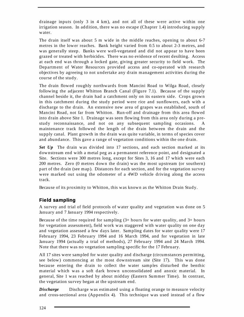
124
drainage inputs (only 3 in 4 km), and not all of these were active within oneirrigation season. In addition, there was no escape (Chapter 1.4) introducing supplywater.
The drain itself was about 5 m wide in the middle reaches, opening to about 6-7metres in the lower reaches. Bank height varied from 0.5 to about 2-3 metres, andwas generally steep. Banks were well-vegetated and did not appear to have beengrazed or treated with herbicides. There was no evidence of recent desilting. Accessat each end was through a locked gate, giving greater security to field work. TheDepartment of Water Resources provided access and co-operated with researchobjectives by agreeing to not undertake any drain management activities during thecourse of the study.
The drain flowed roughly northwards from Mancini Road to Wilga Road, closelyfollowing the adjacent Whitton Branch Canal (Figure 7.1). Because of the supplychannel beside it, the drain had a catchment only on its eastern side. Crops grownin this catchment during the study period were rice and sunflowers, each with adischarge to the drain. An extensive new area of grapes was established, south ofMancini Road, not far from Whitton. Run-off and drainage from this area flowedinto drain above Site 1. Drainage was seen flowing from this area only during a pre-study reconnaissance, and not on any subsequent sampling occasions. Amaintenance track followed the length of the drain between the drain and thesupply canal. Plant growth in the drain was quite variable, in terms of species coverand abundance. This gave a range of vegetation conditions within the one drain.
Set Up The drain was divided into 17 sections, and each section marked at itsdownstream end with a metal peg as a permanent reference point, and designated aSite. Sections were 300 metres long, except for Sites 3, 16 and 17 which were each200 metres. Zero (0 metres down the drain) was the most upstream (or southern)part of the drain (see map). Distances for each section, and for the vegetation surveywere marked out using the odometer of a 4WD vehicle driving along the accesstrack.
Because of its proximity to Whitton, this was known as the Whitton Drain Study.
Field samplingField samplingA survey and trial of field protocols of water quality and vegetation was done on 5January and 7 January 1994 respectively.
Because of the time required for sampling (3+ hours for water quality, and 3+ hoursfor vegetation assessment), field work was staggered with water quality on one dayand vegetation assessed a few days later. Sampling dates for water quality were 17February 1994, 23 February 1994 and 16 March 1994, and for vegetation in lateJanuary 1994 (actually a trial of methods), 27 February 1994 and 24 March 1994.Note that there was no vegetation sampling specific for the 17 February.
All 17 sites were sampled for water quality and discharge (circumstances permitting,see below) commencing at the most downstream site (Site 17). This was donebecause entering the drain to collect the water samples disturbed the benthicmaterial which was a soft dark brown unconsolidated and anoxic material. Ingeneral, Site 1 was reached by about midday (Eastern Summer Time). In contrast,the vegetation survey began at the upstream end.
Discharge Discharge was estimated using a floating orange to measure velocityand cross-sectional area (Appendix 4). This technique was used instead of a flow

125
meter with propeller because the soft sediment made it impossible to maintain theflow meter in a constant position for recording velocity and also because the waterwas often too shallow (< 15 cm) to use a propeller flow meter. A calibration exercisein concrete channels and earthen drains near Griffith compared the orangetechnique with OTT flow meter and found a linear 1:1 response (r2 =0.998) for 10readings. The option of using a flume was discounted as the disturbance causedduring installation of 17 flumes would have changed the drain ecology.
The orange technique was not always effective (see below). Dischargemeasurements were problematic and it was not always possible to measure velocity,even over short distances. At some sites, plant growth became so dense that accessto the permanent site was difficult and risked affecting water quality. This was thesituation for almost the entire length of the drain by 16 March 1994. Similarly, whenthe wind was northerly and strong, it affected the movement of the orange. Thiswas especially noticeable in the lower reaches where the wind was stronglyfunnelled. The first four sites (0-770 metres) were typically ponded water with noflow. Thus for a combination of reasons, the number of readings was limited, andthis restricted the data set available.
Water quality Water samples (500 mL) were taken from mid-stream of eachof the 17 permanent sites following standard procedures (Appendix 4). Dischargewas estimated at the same time and pH and temperature also recorded. Sampleswere stored on ice in the field and transported to the laboratory for initial samplingpreparation on the same day. Samples were analysed for suspended sediments (SS),total phosphorus (TP), filterable reactive phosphorus (FRP), organic nitrogen (asTKN), ammonium nitrogen (NH4), and oxidised nitrogen (NOX). Turbidity (NTU)and conductivity (µS cm-1) were measured immediately on return to the laboratory.
Vegetation surveys Vegetation cover in the wetted area of Whitton drain wasvisually estimated at 100-metre intervals down the drain. This was done by aperson standing on the back of a vehicle (4WD with tray). The 100-metre intervalswere read off the vehicle odometer, always starting from zero at the same place,adjacent to the locked gate at the southern (upstream) end. The area assessed forvegetation cover (the quadrat) was defined by the length of the vehicle (4 metres),but was variable in size because of the variable width of the drain. This samplingintensity and quadrat size gave 4% coverage. During the preliminary studies inJanuary, vegetation cover had been estimated every 200 to 300 metres, giving a 2%coverage or 1-2 quadrats per site, but when the data were plotted, it was apparentthat this was too coarse a resolution.
Vegetation abundance was percent cover within the wetted area of the drain. Totalcover was the sum of two estimates, one for each bank (the vegetation was largelylittoral and the centre of the drain tended to lack vegetation cover, except late in theseason). Open water and mud were not specifically recorded. Cover was percentcover of individual plant species within the quadrat, and the sum of these wasvegetation cover (as a percentage). Plants were identified to level of genus, only, astheir growth-form was considered more relevant to a generic understanding, andcould be more readily linked to plant functional types (PFT).
Data preparation and analysesData preparation and analysesCover Cover for each Site was the mean of 3 quadrats except for the three shorterSites which had only two quadrats (Sites 3, 16 and 17).

126
Downstream nutrient reductions Because assumptions regarding constant flowconditions proved invalid (see Results, below), a 25% rule-of-thumb was used toidentify Site-Site sections suitable for analysis. A section was suitable if discharge atthe downstream site was no less than 75% or no more than 125% of the siteimmediately upstream. As part of this rule, all discharges less than 0.01 m s-1 weretreated as being similar because of the extreme difficulty of measuring flow andcross-sectional area at 10 cm intervals in narrow, silty, vegetated channels. For twosites where discharge was missing (Sites 7 and 12 on 17th February), the definition of‘immediately’ upstream was extended (ie Sites 6-8 and 11-13) giving a distance of600 metres.
Nutrient reduction was the difference between up and down sites, first based ondifferences in estimated loads then, as a cross-check, on concentrations. Correlationanalysis (Pearson) was used to explore the relationship between change in load andtwo key factors, mean vegetation cover and velocity, for each nutrient individually.Bartlett’s chi-square analysis was used to test the significance of the correlationcoefficient.
Data were analysed using SYSTAT.
7.37.3 ResultsResults
General observationsGeneral observationsDischarges into Whitton Drain Only two of the side-drains entering WhittonDrain were observed to flow when visited during January–March 1994. These wereinflow from a rice crop between Sites 4 and 5 (at 975 metres) and inflow from asunflower crop between Sites 8 and 9 (at 2220 metres). Relevant field observationsare summarised below (Table 7.1).
The drains which were not seen flowing were one between Sites 10 and 11, whichwas for pasture, and the road-side drain near Site 17 from Wilga Road would haveflowed only after rainfall and would have carried road run-off. Although there wereno observations of drainage from the grape crop upstream of Site 1, it was believedto have discharged into the drain from time to time. For example, on 17th Februarythere was downstream flow at Site 3 (above the drain from the rice crop). This couldhave been drainage from the area under grapes but equally could have been returnof backed-up water caused by inflow from the rice crop. By the 16th March, thewater depth in this part of Whitton Drain had fallen due to the combined effects ofevapo-transpiration and reduced in-flows at Site 4-5.
Biota Carp were seen swimming and feeding in the drain on most field visits, andwere particularly evident in the lower reaches. This was due either to a diurnalmovement or to their enhanced conspicuousness here (less vegetation). It seemedthat carp were moving upstream in the morning and downstream in the afternoon,but no systematic observations were done to confirm this was a behavioural pattern.
Periodic chemical contamination was implicated as on some visits carp were dead,whilst on others they were alive. Thus on 5 January, all the carp seen were alive,and these numbered 1, 2 or 3 carp at each of five Sites. However, on 8th February1994 several dead carp were noted just below and above the rice in-flow near Site 4,and one dead carp at Site 9 but further downstream there were several alive at Site16. Similarly, on 17 February, there were many live carp at Site 10. But on 23rd

127
February, dead carp, including some juveniles, were seen at Sites 10, 12 and 13.Again on 16 March, live carp were seen, but only at the lowest site, Site 17.
The cause of carp death was not determined, but chemicals specifically endosulfansulfate is suspected. Chemicals detected in MIA drains in February, based on foursuccessive years sampling (Appendix E), include endosulfan sulfate which is knownto be used in the general area of Whitton (Lillian Parker, Murrumbidgee Irrigation,pers. comm. 1998). Carp are known to be sensitive to endosulfan but theirsensitivity to other chemicals detected in February is not specifically known.
Hydrology The longitudinal profiles of velocity and discharge (Figure 7.2)showed these were not constant, as expected. In addition, there were markeddifferences between sampling dates.
At the top of the drain, the water was usually ponded, hence velocity and dischargewere generally very low for Sites 1 to 4. Downstream of Site 4, however, bothvelocity and discharge increased sharply. In part this was due to drainage enteringthe drain (Table 7.1), and in part to the funnelling effect of dense edging vegetation.Velocity tended to increase down the drain, and on both dates in February reachedits maximum of 0.2-0.3 metres s-1 at Site 14, then decreased rapidly at Sites 15 and16. Velocity was similar for both sampling dates in February, ranging from 0.1-0.3metres s-1 but was much lower in March, less than 0.1 metres s-1 (Figure 7.2, top).Velocity at Site 17 was higher because here flow passed under a road bridge.
Surges of off-farm drainage appeared to occur twice, as indicated by distinctdischarge peaks, one at Sites 4 and 5 on 17th February, and one between Sites 8 and 9on 23rd February (Figure 7.2 bottom). On 17 February, discharge peaked at about 0.2m3 s-1 at Sites 6-7, suggesting drainage had recently been discharged from the ricefield, an interpretation that was consistent with field observations (Table 7.1). Thehigh discharge plotted for Site 12 is probably an erroneous velocity reading (and hasbeen removed from subsequent plots) as it was not supported by field observationsof discharge. On 23 February, there was discharge peak of 0.14 m3 s-1 at Sites 9 and10, which was consistent with field observations of discharge from the sunflowercrop between Sites 8 and 9 (Table 7.1). At other sites in this middle section of thedrain, discharge was consistent 0.9-0.10 m s-1.
Discharge patterns varied between the three dates, being highest on 17 February andlowest, almost negligible on 16 March (Figure 7.2 bottom). On both sampling datesin February, discharge appeared to decrease downstream of Site 14. Reasons for thisare not certain. This may have been due to the very different conditions (denselyvegetated versus almost bare) and the challenge of estimating velocity and cross-sectional area at 10 cm intervals across channels which were relatively wide, withshallow water over deep silt.
Aquatic characteristics On each visit, an upstream-downstream difference of5-6oC from Site 17 to Site 1 was recorded. This was, in fact, an increase due todiurnal heating (Figure 7.3 top left) and it tracks the times of sampling. Largediurnal shifts in temperature were noted earlier in Main Drain J, a much larger anddeeper drain showing an increase of 10 degrees during winter (Figure 6.3).
Diurnal shifts in other parameters were not apparent. During February, there wasno obvious diurnal shift in pH which was generally less than neutral. This was inmarked contrast to measurements made during the preliminary survey on 5January, when the pH down the drain ranged from 8.8 at the top of the drain to 10.4at the bottom. It was also higher in March, when pH ranged between 7 and 9

128
(Figure 7.3 top right). This was a time of very shallow water, and algal films on thebenthos. The relatively low and unchanging pH suggested minimal in-situphotosynthesis in February was therefore anomalous and may have been linked tocarp mortality. This lack of algal activity was supported by relatively lowconcentrations of dissolved oxygen at Sites 6 – 17, for February only (Figure 7.3bottom left). Oxygen levels were consistently very low at Site 3, and low at the sitesimmediately adjacent. Conductivity ranged from 140 to nearly 200 µS cm-1 andtended to increase downstream by 10-40 µS cm-1 on each sampling date (Figure 7.3bottom right). Conductivity tended to increase down the drain. One explanation forthis, a slight concentration effect, due to evapo-transpiration from the water surfaceunder hot windy conditions of summer, does not readily match discharge data.
Algae Algae were not sampled but some pertinent field observations weremade. On 8 February, dark green filamentous algae was noted at Site 6, benthicalgae were evident at Site 14, and there was a build-up of floating algae on the fencenear Site 16. Similar observations were made on 23 February, when it was notedthat the water was relatively clear in the lower reaches, and that at Sites 14 and 16benthic algae were evident, and that dislodged patches were floating downstream atmidday. In addition, there were floating red algae at Site 1.
Nutrient concentrationsNutrient concentrationsNutrient concentrations down Whitton Drain showed greater variability thanexpected, both down the drain and between sampling dates (Figures 7.4 and 7.5).
17th February 1994 Concentrations of SS down the drain were fairly constant,ranging between 30-50 mg L-1, apart from a high value of 142 mg L-1 in the upstreamponded section. Phosphorus concentrations were generally lower than theanalytical threshold (not shown), suggesting considerable dilution had occurred andthat the SS was inorganic. Concentrations of NOx and NH4 increased steadily fromSite 5 to Site 17. Organic nitrogen dominated nitrogen concentrations, which wasconsistent with BR-100 and BR-50 water quality signature (Table 3.5). TKNconcentrations in the drain ranged from 0.76 at Site 5 to 0.97 mg L-1 at Site 16, with apronounced peak of 1.51-1.57 mg L-1 at Sites 8 and 9 (this is not evident in thegraphs, as the plotting package has distorted the relative values).
In summary, nutrient and sediment concentrations were consistently high in theponded section upstream of Site 5; and water quality downstream of Site 5, withvery low (undetectable) levels of phosphorus concentrations and with total nitrogenlargely composed of organic nitrogen were consistent with drainage from ricefields.Nutrient concentrations did not change down the drain in any way that suggested asystematic improvement due to the drain environment or to water plants, and therewas a general increase in NH4 and NOx.
23 February 1994 Flow regime again determined much of the variations evidentin water quality. The ponded section upstream of Site 5 had the highestconcentrations of SS (> 50 mg L-1), the highest concentrations of TP, (> 0.1 mg L-1)and included the highest concentrations of NOx and NH4 (Figure 7.5).
The discharge peak at Sites 9 and 10 (Figure 7.2) had a distinctive water quality.This was a small increase in FRP (to 0.05 mg L-1, equivalent to the ponded section), alarge increase in TKN (reaching more than 1.50 mg L-1 and far exceeding the pondedsection) and a sharp increase in NOx (reaching 0.13-0.18 mg L-1, similar to levels in

129
the ponded section). Discharge at Sites 9 and 10 had no noticeable effect on SS or TP(Figure 7.5 top left).
Vegetation surveysVegetation surveysFive plant functional types were present: emergent Monocots, emergent Dicots,floating leafed aquatics, submersed aquatics and mat-forming grasses. The numberof species in each type ranged from 1 to 5 (Table 7.2), there being two species ofJuncus in the emergent Monocot group. The plant type with the most number ofspecies was emergent dicotyledonous plants.
Vegetation cover was patchy down Whitton Drain. In late January, cover rangedfrom 2 to 92% (Figure 7.6 top). Areas of dense cover (arbitrarily defined as > 60%cover) occurred at 450-700 metres (Site 3), 1475-1850 metres (Sites 6 and 7) and at2600-2850 metres (Site 10). Areas of sparse (<20%) cover were 0-200 metres (Site 1),2100-2350 metres (Sites 8-9), 2950-3100 metres (Site 11) and 3600-4300 metres (Sites13-17). The dominant functional types were the two emergent forms, particularlythe emergent monocots, and the mat-forming grasses (Figure 7.6, middle andlower). The fully aquatic forms, the submerged and the floating leafed plants, werepresent only in small or trace quantities except for one patch 700 metres down thedrain (ie within the ponded area at Site 3).
Abundance increased during the two study months due mainly to late summergrowth of the emergent herbs (Table 7.3). Although this occurred throughout thedrain (Figure 7.7), the overall pattern of alternating patches of high or low coverremained, with low cover in the top ponded section and in the lowest section. Therewas extensive death of one species, the milfoil Myriophyllum sp., in the lowerreaches. This was first noticed between Sites 8 and 9 on 23 February and themortality then spread downstream and by 24 March there was very littleMyriophyllum left alive. Again, this mortality is consistent with a other observationsof biocide. Although grouped as an emergent Dicot, milfoil was one of the fewspecies generally recognised as an aquatic, and had submerged leaves.
The cover of the aquatic plant types with submerged and floating leaves remainedlow throughout the study period (Table 7.3) and was restricted to specific areas,Sites 2-3 (in the ponded section at the top of the drain) and also Sites 8-9-10 and Sites12-13-14. The expectation had been that submerged and floating-leafed aquaticswould become more abundant through summer, either because of increased growthor because of shallower water making them more conspicuous.
Field notes for 23 February note that Persicaria and Paspalum distichum were coveringmore than half the drain at sampling sites 12, 13, 14 causing channelised flowbetween the vegetation mats.
Drain sectionsDrain sectionsBased on total cover, the distribution of certain species and functional types, andincluding some broad hydrological differences, it is possible to recognise fourdistinctive sections in Whitton Drain during February-March (Table 7.4): theponded section at the head of the study area; the section affected by rice drainageonly; the section affected by sunflower and rice drainage; the bottom section, whichwas wide and shallow and had deep silt.

130
Changes in water qualityChanges in water qualityThe application of the 25% rule reduced the number of comparisons from potentially48 comparisons (17 sites giving 16 up-down comparisons on 3 days) to only 16: ninecomparisons for water quality data for 17th February, four for 23rd February andthree for 16th March.
The effect of the drain on nutrient loads was ‘beneficial’ but not strongly so (Table7.5). A tally of all possible comparisons gives 64 instances of nutrient load reductionversus 45 of increase and 3 ‘n.m.’ (not measured). There were two Site x Datecombinations with no nutrient reduction recorded for any of the seven nutrientforms, Site 15-16 on 17 February and Site 7-8 on 16 March. The nutrients showingthe most frequent reduction in loads were FRP, TN and TKN (on 10 out of 16instances). However, a sample size of 16 is rather small to be confident that afrequency of 10 represents a significantly greater performance than a frequency of 9(for SS) or of 8 (TP and NOx).
If flow is virtually unchanged between consecutive Sites (as implied by the 25%rule), then changes in nutrient concentrations are an equally valid way to investigatethe effectiveness of the drain. Using the same Site x Date combinations,concentrations showed a similar trend as for loads, that is only a marginal benefit(Table 7.6). In this case, there were 49 instances of nutrient concentration reductionversus 40 of concentration increase, plus 19 instances of no detected change and 4‘n.m.’. Only one Site x Date combination showed no nutrient reductions at all, Site13-14 on 16 March. The nutrient forms showing the most frequent reductions inconcentration were TN, TKN and SS (with 8 out of 16 instances), whereas TP had theleast frequent.
Changes in nutrient load from one Site to the next did not correlate with meanvegetation cover. Correlation coefficients ranged from –0.40 for NH4 to <0.001 forNOx and none were significant (Bartlett’s chi-square statistic). Velocity was ofgreater importance as a factor influencing changes in nutrient load but wassignificant only for TP with a correlation coefficient of 0.55 (p = 0.03). A scatterplotof net change in TP load against velocity (Figure 7.8) shows clearly there is atransition from deposition to entrainment. Although the plot shows that the criticalvelocity is about 0.15 m s-1, this should not be taken as a definitive and absolutevalue because of the simple way that velocity was measured, and the scatter in thedata. Nonetheless, it does indicate that low velocity is favourable.
7.47.4 DiscussionDiscussionWhitton Drain was chosen as the closest approximation to an ideal drain (seeIntroduction) and was expected to have minimal variability. Yet it was apparentthat even here, there was considerable spatial (the four sections) and hydrologicvariability (the ponded section and the two surges).
The ponded section at the top of the drain was distinctive (Table 7.4) because of itshigh nutrient concentrations, very high SS, low plant cover with a patch of thesubmerged aquatic Vallisneria americana. Low to zero flows meant this section wasvirtually isolated from the rest of the drain. The presence of V. americana and ofPotamogeton tricarinatus, which are perennial macrophytes and obligate aquatics,suggests this was a near permanent ‘waterhole’. Reasons for the high turbidity wasnot determined but bioturbation by carp or water birds is possible. The low oxygen

131
levels and high NH4 levels suggest that this was also an area of intense biologicalactivity.
The two hydrological surges were characterised by water that was clear, low inphosphorus but high in nitrogen forms. This is typical of rice drainage.
Although this variability compromised the original sampling design, and althoughthe data are sparse, the overall conclusion from the 16 data points for each nutrient(Tables 7.5 and 7.6) is that Whitton Drain did improve water quality. However, thebeneficial effect was not strong and not consistent, and could not be statisticallylinked to measures of vegetation abundance. These findings are less optimistic thanexpected and not supported by previous work on nutrient interception in irrigationdrains (Bowmer et al. 1994). On the positive side, however, is that an effect wasdetected when nutrient concentrations were relatively low. General experience isthat the beneficial effects of plants on water quality is most marked (or detected)when concentrations are high (Faafeng and Roseth 1993).
Micro-processesMicro-processesVelocity determines whether particles are entrained or deposited, and the criticalvalue at which these occur depends on particle size. Unconsolidated silts and claysare entrained by velocities of 0.01-0.02 m s-1 whereas velocities of approximately 0.15m s-1 are approaching turbulent flows and can be expected to entrain gravels andpebbles (Reynolds 1996). Flow velocities measured in Whitton Drain were high and,despite the promising calibration with the Ott meter, may have been overestimates.Possibly this is because a single value correction factor, such as 0.85 suggested byGordon et al. (1992) is unlikely to be valid for the range of vegetation cover, widthand depth encountered in Whitton Drain.
Although the absolute velocity (and discharge) values obtained in the Whitton Drainstudy can be questioned, the finding that velocity was a significant factor and thatthere was a critical threshold was in agreement with theory (Reynolds 1996).Moreover, the velocities in Whitton Drain were frequently above the empirically-determined threshold of 0.15 m s-1 (Figure 7.2), indicating that entrainment was,overall, more likely than deposition. It was not clear why SS was not similarlyaffected.
The presence of carp in Whitton Drain was both a factor affecting water quality (cfbioturbation, Chapter 6) and an indirect indicator of water quality. While foraging,live carp disturb sediments or dislodge loose material from leaves of plants in thelittoral zone. Although care was taken to avoid them, there was no means ofguaranteeing that a water sample had not been affected by carp foraging – or bywaterbird activity - further upstream.
Carp are tolerant of a range of water conditions but are sensitive to pesticides andherbicides used in irrigated agriculture and in irrigation drains (eg Bowmer et al.1994). As Whitton Drain was not subject to weed control during the study period,the presence of dead carp on 8th February and on 23rd February, indicates pesticideactivity. Pathways for pesticides into drains are crop run-off and over-spray or drift.Contamination of this sort is likely to affect other biota and may explain the curiouslack of photosynthetic activity in the drain during February, as indicated by theinvariant and low pH and oxygen levels and dieback of milfoil (Figure 7.3). Periodicpulses of contamination would also limit the abundance of micro-organisms inWhitton Drain, whether on or in the sediment, or epiphytic on plants, and reducebiological activity, and restrict nutrient improvement.

132
The dominant plant functional types in Whitton Drain were emergent Monocots,emergent Dicots and mat-forming grasses. These have leaves that are aerial, ratherthan submerged, and hence that their primary method of nutrient uptake is viaroots. Such plants are less likely to be affected by biocide-contaminated drainage.Plants in Whitton Drain were not specifically inspected to assess their role as asubstrate, but their epiphytic growth, if present, was not obvious. Hence onenutrient-removing process, ie the uptake of soluble nutrients, was probably limited.
Thus of the several processes whereby vegetation could reduce nutrient load,directly or indirectly, only one (deposition) appeared to be happening, and only to alimited extent. Although the evidence is not strong, it appears that the otherprocesses were of limited importance in Whitton Drain. The drain lackedsubmerged and floating-leafed plants with submerged leaves which could take upsoluble nutrients, FRP and NOx, or act as a substrate for those epiphyticcommunities. The abundance of epiphytic fauna and of heterotrophic microbialcommunities was probably being reduced by periodic pulses of pesticides. In turn,this would limit microbe-dependent processes such as nitrification and de-nitrification. Persistent high turbidity may limit development of a benthic algae, andhence limiting this nutrient uptake pathway as well.
Suspended sediments are not normally considered a water quality issue but in anirrigation area they are an important vehicle for transporting adsorbed nutrients,including bacteria, and some chemicals. Thus there could be capacity to increaseresidence time in some drains and hence slow the export of pesticides and increasethe opportunity for break-down.
High velocity, few plants and especially few submerged plants, periodic pulses orspills of pesticides, and sustained high turbidity: these characteristics are not uniqueto Whitton Drain. The effectiveness of irrigation drains in improving water qualitywill require encouraging and maintaining a biological environment that is suitablefor plants with submerged leaves, their epiphytic fauna and benthic microbes. Theideal drain characteristics proposed when searching for a field site (see above) areprobably useful guides for managers. However, of the several characteristics listed,only one (velocity) was empirically demonstrated to be important. Unfortunately,this was probably the one most difficult to measure under the specific fieldconditions so the critical values deduced from this need to be confirmed.
Other design criteria, specifically those relating to vegetation, such as abundance,the importance of different structures or species, were not resolved in this study,because of the drastically reduced data set, from 48 to 16 comparisons.
FindingsFindingsThe ideal drain chosen for investigation, the Whitton Drain, proved to be less thanideal, for a number of reasons: high flows, low nutrient concentrations and anapparent biocide.
♦ Despite sub-optimal conditions, this SO1 drain was effective in improving waterquality overall, most noticeably in relation to FRP, TN and TKN (if based onloads) and on TN, TKN and SS (if based on concentrations).
♦ A critical velocity was detected under field conditions above which TPentrainment occurred and below which TP appeared to be deposited

133
Principal recommendation arising from the Whitton Drain Study
♦ As water quality improvement by in-channel biological processes requires anintact and functioning biological community, every effort should be made toprotect and safe-guard the drain environment.
♦ Biological treatment within drains should be promoted by encouraging smallgroups of farmers within a sub-catchment.
♦ The ideal drain characteristics appear to be a reasonable guide but specificcriteria relating to plant cover and functional types need to be developped.These would need to be done in consultation with an engineer and a hydrologist.
♦ The beneficial effects of increasing residence time and encouraging sedimentdeposition on agricultural chemicals needs to be specifically investigated.
♦ The effect of sustained land and drain management practices that affect thequantity and composition of drain sediments, such as de-silting and bioicides indrainage, need to be determined by focusing on benthic processes, specificallythe rate of nitrogen transformations in benthic sediments and the importance oforganic material.

134
ReferencesReferences
Bowmer, K.H., Bales, M. and Roberts, J. (1994). Potential use of irrigation drains aswetlands. Water Science and Technology 29:151-158.
Faafeng, B.A. and Roseth, R. (1993). Retention of nitrogen in small streams artificiallypolluted with nitrate. Hydrobiologia 251: 113-122.
Gordon, N.D., McMahon, T.A. and Finlayson, B.L. (1992). Stream hydrology: an introductionfor ecologists. John Wiley & Sons, Chichester.
Harris, G.P. (1996). Catchments and aquatic ecosystems: nutrient ratios, flow regulation andecosystem impacts in rivers like the Hawkesbury-Nepean. CRC-FE Discussion paper.June 1996.
Howard-Williams, C. (1985). Cycling and retention of nitrogen and phosphorus in wetlands:a theoretical and applied perspective. Freshwater Biology 15: 391-431.
Jansson, M., Leonardson, L. and Fejes, J. (1994). Denitrification and nitrogen retention in afarmland stream in southern Sweden. Ambio 23(6);326-331
Raisin, G.W., Mitchell, D.S. and Croome, R.L. (1997). The effectiveness of a smallconstructed wetland in ameliorating diffuse nutrient loadings from an Australianrural catchment. Ecological Engineering 9:19-35.
Reynolds, C.S. (1996). Algae. Chapter 2 in: River Biota: Diversity and dynamics. Eds G.Petts and P. Calow. Blackwell Science. Oxford.
Svendsen, L. M and Kronvag, B. (1993). Retention of nitrogen and phosphorus in a Danishlowland river system: implications for the export from the watershed. Hydrobiologia251: 123-135.

135
Table 7.1 In-flows to the Whitton study drain
Summary of field observations of inflows into Whitton Drain made during visits for trials,setting-up and sampling runs.
Date (1994) In-Flows
5 January From rice crop, ie between Sites 4-5
17 February From rice crop, ie between Sites 4-5;Also downward from Site 3
23 February From sunflower crop, ie between Sites 8-9No in-flow further up
16 March Very slow flow observed from Sites 4-5 downwards.No other in-flows
Table 7.2 Growth-forms of plants recorded in Whitton Drain
Growth-forms is used here to describe the plants and as a means of indicating their likelyfunctional type. Several schemes of plant functional types have been proposed, with thefunction emphasised depending on the questions being posed. Edge species are listed herefor completeness but occurred only in trace amounts, and were too infrequent and of toolow cover to make a contribution to total cover.
EmergentMonocots
EmergentDicots
Floating-leafed
Aquatics
SubmersedAquatics
Mat-formingGrasses
Edgespecies
Juncus (twospecies)
Cyperus
Typha
Paspalumdilatatum
Myriophyllum
Sagittaria
Persicaria
Pratia
Potamogetontricarinatus
Vallisneriaamericana
Paspalumdistichum
Cynodondactylon
Rumex crispus
5 4 1 1 2 1

136
Table 7.3 Changes in vegetation January to March
Summary of changes to abundance of species in Whitton Drain, organised by the five maingrowth types. Abundance is the mean and median values of all quadrats.
Plant Cover Late January(%)
27 February(%)
24 March(%)
Total Cover MeanMedian
32.718.0
27.632.0
39.343.3
Emergent Mono MeanMedian
12.97.0
7.07.0
4.94.3
Emergent Herbs MeanMedian
10.33.5
15.512.0
23.725.0
Mat Grasses MeanMedian
6.50.5
4.43.0
6.35.7
Floating Leaf MeanMedian
1.0<0.01
0.4<0.01
1.0<0.01
Submerged MeanMedian
2.0<0.01
0.4<0.01
3.5<0.01
Table 7.4 Ecological zones in Whitton Drain
Characteristics of the four zones recognised in Whitton Drain, based on hydrological andplant characteristics.
Section
0 to 1000 metresSites 1 - 4
Water ponded. Upstream of inflow from ricefield.Cover low in areas dominated by emergent monocots anddicots, with a persistent patch of submerged and floatingleafed plants.
1000 to 2100 metresSites 5 - 8
Immediately below in-flow from rice-field but above in-flow from sunflower crop.Cover generally high, dominated by emergent monocotsand dicots, and mat-forming grasses, Paspalum distichum,Persicaria and Myriophyllum.
2100 to 3800 metresSites 9 - 14
Immediately below in-flow from sun-flower crop.Includes the high velocity Site 14Cover generally high except for an area around Site 11,mainly Paspalum distichum, Persicaria and Myriophyllum.
3900 to endSites 15 - 17
No inflows. Shallow water, deep silt, wide channel withlow cover. Vegetation mostly limited to sparse littoralfringe of Juncus spp, Paspalum dilatatum and Persicaria,with a small patch of Vallisneria.

137
Table 7.5 Changes in nutrient loads: between sites
Positive and negative changes in SS loads (g s-1) and nutrient loads (mg s-1) betweencontiguous Sites down Whitton Drain for three dates in summer 1994. Criteria for selectingthese Site x Date combinations are explained in the text. Distances between sites was 300metres, except where indicated (**). Positive indicates a gain (undesirable in terms of waterquality) and negative indicates a loss (desirable).
17 February 1994
Sites SSg s-1
TPmg s-1
FRPmg s-1
TNmg s-1
TKNmg s-1
NOxmg s-1
NH4mg s-1
3-4 -4.57 -6.72 -0.17 -60.09 -55.55 -4.54 -6.12
5-6 -4.35 -2.68 5.90 -20.0 -20.0 -1.70 -3.62
6-8 (**) 3.54 2.35 1.52 -50.0 -40.00 -2.35 1.55
9-10 -0.89 0.84 -0.80 60.0 56.94 -3.91 -1.27
10-11 2.00 1.69 -0.38 -10.0 -6.94 1.40 1.68
11-13 (**) -1.75 -3.27 0.24 -60.0 -50.0 -4.84 -2.49
13-14 -0.14 0.25 -1.43 74.46 73.57 -4.60 -4.18
14-15 1.20 2.69 -0.30 -2.01 -7.46 5.45 4.28
15-16 0.49 0.52 1.70 5.32 3.90 1.42 1.31
23 February 1994
Sites SSg s-1sec
TPmg s-1
FRPmg s-1
TNmg s-1
TKNmg s-1
NOxmg s-1
NH4mg s-1
9-10 2.24 1.63 -1.66 20.0 20.0 8.04 -14.39
11-12 0.28 -0.90 0.42 -5.53 -8.98 3.46 0.56
12-13 -0.28 -0.06 -0.58 -0.83 -1.02 0.18 -0.78
13-14 -0.25 -0.24 -0.08 14.02 13.85 0.17 -0.12
16 March 1994
Sites SSg sec s-1
TPmg s-1
FRPmg s-1
TNmg s-1
TKNmg s-1
NOxmg s-1
NH4mg s-1
6-7 -0.51 -2.20 -0.61 -21.58 -20.98 -0.61 n.m.
7-8 0.38 1.85 0.02 17.77 17.75 0.02 n.m.
13-14 -0.68 -1.94 -0.39 -20.85 -20.46 -0.39 n.m.

138
Table 7.6 Changes in nutrient concentrations: between sites
Positive and negative changes in SS concentrations (g L-1) and nutrient concentrations (mg L-
1) between contiguous Sites down Whitton Drain for three dates in summer 1994. Criteriafor selecting these Site x Date combinations are explained in the text. Distances betweensites was 300 metres, except where indicated (**).
17 February 1994
Sites SSg L-1
TPmg L-1
FRPmg L-1
TNmg L-1
TKNmg L-1
NOxmg L-1
NH4mg L-1
3-4 -85.6 -0.11 0.01 -0.64 -0.69 0.05 -0.08
5-6 -16.4 -0.01 n.m. -0.01 0 -0.01 -0.01
6-8 (**) 13.2 0.01 0 -0.36 -0.33 -0.02 0
9-10 -11.2 0 -0.01 0.26 0.3 -0.04 -0.02
10-11 8.4 0 -0.01 -0.31 -0.30 -0.01 0
11-13 (**) -8.0 -0.01 0.01 -0.22 -0.24 -0.02 -0.01
13-14 3.6 0.01 -0.01 0.70 0.72 -0.02 -0.02
14-15 -2.4 0.01 -0.02 -0.30 -0.30 0 0.01
15-16 -1.6 0 0.01 -0.13 -0.12 -0.01 0
23 February 1994
Sites SSg L-1
TPmg L-1
FRPmg L-1
TNmg L-1
TKNmg L-1
NOxmg L-1
NH4mg L-1
9-10 14.4 0.01 -0.01 0.11 0.06 0.05 -0.11
11-12 4.8 -0.01 0.01 0.01 -0.03 0.04 0.01
12-13 -2.8 0 -0.01 0.01 0 0 -0.01
13-14 -1.6 0 0 0.18 0.18 0 0
16 March 1994
Sites SSg L-1
TPmg L-1
FRPmg L-1
TNmg L-1
TKNmg L-1
NOxmg L-1
NH4mg L-1
6-7 30 0.07 0.03 -0.18 -0.21 0.03 n.m.
7-8 13 0.02 -0.04 0.60 0.51 0.09 n.m.
13-14 17 0.02 0.02 0 0 0 n.m.

139
Figure 7.1 Whitton Drain
Map showing principal features of the Whitton Drain site and adjacent land uses.
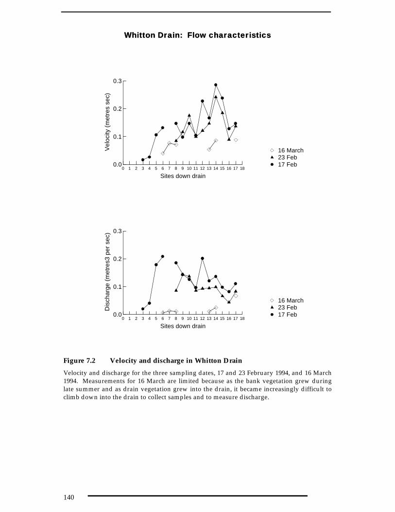
140
Whitton DrainWhitton Drain: Flow characteristics: Flow characteristics
0 1 2 3 4 5 6 7 8 9 10 11 12 13 14 15 16 17 18
Sites down drain
0.0
0.1
0.2
0.3
Vel
ocity
(m
etre
s se
c)
17 Feb23 Feb16 March
0 1 2 3 4 5 6 7 8 9 10 11 12 13 14 15 16 17 18
Sites down drain
0.0
0.1
0.2
0.3
Dis
char
ge (
met
res3
per
sec
)
17 Feb23 Feb16 March
Figure 7.2 Velocity and discharge in Whitton Drain
Velocity and discharge for the three sampling dates, 17 and 23 February 1994, and 16 March1994. Measurements for 16 March are limited because as the bank vegetation grew duringlate summer and as drain vegetation grew into the drain, it became increasingly difficult toclimb down into the drain to collect samples and to measure discharge.

141
Drainage: Physical characteristicsDrainage: Physical characteristics
0 2 4 6 8 10 12 14 16 18Permanent Sites: 1 - 17
15
20
25
30T
empe
ratu
re
0 2 4 6 8 10 12 14 16 18Permanent Sites: 1 - 17
5
6
7
8
9
pH u
nits
0 2 4 6 8 10 12 14 16 18Permanent Sites: 1 - 17
0
2
4
6
8
10
Oxy
gen
(mg
L-1)
0 2 4 6 8 10 12 14 16 18Permanent Sites: 1 - 17
100
120
140
160
180
200
Con
duct
ivity
(m
icro
S c
m-1
)
Figure 7.3 Aquatic environment in Whitton Drain, summer 1994
Longitudinal profiles of the aquatic environment for three dates in summer 1994:temperature, pH, oxygen and conductivity. Conductivity was measured in laboratory onreturn from the field, but all others were measured in the field.
KEY Solid circles, 17 February; hollow triangle, 23 February; solid diamond, 26 March.

142
Whitton Drain, 17 February 1994Whitton Drain, 17 February 1994: Nutrient Concentrations: Nutrient Concentrations
0 2 4 6 8 10 12 14 16 18Permanent Sites: 1 - 17
0
50
100
150
Sus
pend
ed S
edim
ents
(m
g L)
0 2 4 6 8 10 12 14 16 18Permanent Sites: 1 - 17
0.0
0.1
0.2
0.3
0.4
0.5
Nitr
ogen
(m
g L)
0 2 4 6 8 10 12 14 16 18Permanent Sites: 1 - 17
0
1
2
3
4
Nitr
ogen
(m
g L)
Figure 7.4 Water quality in Whitton Drain
Longitudinal profiles of nutrient concentrations down Whitton Drain, 17 February 1994.
KEY SS (top); ammoniacal and oxidised nitrogen, being circles and triangles respectively(middle), and organic and total nitrogen (bottom).

143
Whitton Drain, 23 February 1994Whitton Drain, 23 February 1994: Nutrient Concentrations: Nutrient Concentrations
Suspended Sediments
0 2 4 6 8 10 12 14 16 18Permanent Sites: Sites 1 - 17
0
50
100
150
Sus
pend
ed S
edim
ents
(m
g L)
Phosphorus
0 2 4 6 8 10 12 14 16 18Permanent Sites: Sites 1 - 17
0.0
0.05
0.10
0.15
0.20
Pho
spho
rus
(mg
L)
Nitrogen
0 2 4 6 8 10 12 14 16 18Permanent Sites: Sites 1 - 17
0.0
0.05
0.10
0.15
0.20
Nitr
ogen
(m
g L)
Nitrogen
0 2 4 6 8 10 12 14 16 18Permanent Sites: Sites 1 - 17
0.0
0.5
1.0
1.5
2.0
Nitr
ogen
(m
g L)
Figure 7.5 Water quality in Whitton Drain
Four longitudinal profiles of water quality down Whitton Drain for 23 February 1994.
KEY SS (top left); TP and FRP (top right); NH4 and NOx, being triangle and circlerespectively (bottom left); TKN and TN (bottom right)..

144
Total Cover
0 1 2 3 4 50
20
40
60
80
100
Veg
etat
ion
Cov
er (
%)
Emergent Macrophytes
0 1 2 3 4 50
20
40
60
80
100
Veg
etat
ion
Cov
er (
%)
Mat-Forming Grasses
0 1 2 3 4 5Distance down Whitton Drain (km)
0
20
40
60
80
100
Veg
etat
ion
Cov
er (
%)
Figure 7.6 Vegetation in Whitton Drain in January 1994
Longitudinal profiles of vegetation abundance (measured as cover) for all species, and thedistribution of two of the five growth-forms, emergent Monocots, and mat-forming grasses.

145
0
1
2
3
4
5
6
7
8
9
10
11
12
13
14
15
16
17
18
Per
man
ent S
ites:
1 -
17
0 20 40 60 80 100Vegetation Cover (%)
24 March27 Feb
Figure 7.7 Vegetation changes February to March
Changes in total vegetation cover at the 17 permanent sites down Whitton Drain during latesummer. Sampling dates are 27 February and 24 March
0.0 0.1 0.2 0.3Velocity (m sec)
-10
-5
0
5
Cha
nge
in lo
ad o
f TP
(m
g se
c)
Figure 7.8 Effect of velocity on change in TP load
Change in TP load (mg sec) down a 300-metre section of the Whitton Drain moves fromnegative (deposition) to positive (entrainment) at higher average velocities. Data points inthis were assumed to have relatively stable flows at the time of measurement, as determinedby the 25% rule (see text). Velocity measurements were done simply, so it is the trend,rather than the absolute values, that is of importance.

146
Chapter 8Chapter 8
Synthesis and FindingsSynthesis and Findings
Stream ordering and drain classificationStream ordering and drain classificationThe usefulness of stream ordering as a classification system for irrigation drains wasinvestigated by applying the Strahler system at increasingly larger spatial scales,from local (Pilot Study) to regional (Mirrool Study) and then across irrigation areaswithin the Murray-Darling Basin (Basin application). The scale of investigation thusincreased from two sub-catchments south of Griffith (Pilot Study), to thirteen sub-catchments within the Mirrool Irrigation Area (Mirrool Study) to seven sub-catchments in other irrigation areas in southern part of the Murray-Darling Basin(Basin application).
The range of stream orders that resulted from applying the Strahler system to anirrigation area was limited, and only stream orders one to three (SO1 to SO3) werepresent in abundance. Order four drains (SO4) were generally the main exit drains,at least in irrigation areas in New South Wales. These are discussed further below(SO4 drains).
To be effective, a classification system should produce discrete classes, ie eachstream order should be distinctive. The Pilot Study found that mean values for eachof the morphologic and hydrologic characteristics were quite variable, and hence itwas not possible to consistently distinguish between SO1 and SO2 drains based on asingle one of these characters. This variability was reduced by including catchmentsize and land use. The expectation that these factors would affect discharge andwater quality, respectively, as in natural systems, was found to be true, and thecombination of land use and Strahler stream order was an effective summary ofphysical and chemical drain characteristics. Biological characteristics were not sowell classified and this was attributed to a history of weed control.
Whereas physical, ie morphological and hydrological, characteristics increaseddownstream, this was not always true for chemical and biological characteristics.For example, SO1 drains in horticultural areas had the highest mean vegetationcover (Table 2.6); conductivity was fairly constant in SO1, SO2 and SO3 drains inbroadacre catchments but was highest in SO1 drains in horticultural catchments andtended to decrease downstream (Table 2.4).
Land use resulted in distinctive chemical signatures in irrigation drainage, henceland use could be used to summarise catchment differences in water quality. Landuse, however, did not capture longitudinal differences so needed to be combinedwith stream order. This combination was effective in discriminating types in otherirrigation areas and hence in facilitating comparisons between irrigation areas.Although the sample size used was not large, it showed that stream ordercharacteristics differed between irrigation areas, and that the characteristics observedin a particular class of drains in the Mirrool Irrigation Area did not match otherirrigation areas.

147
Recommendation: Stream order and land use be used together as a basis for aphysical classification of irrigation drains and catchment attributes be used todescribe and summarise irrigation areas.
Effectiveness of vegetated drainsEffectiveness of vegetated drainsThe effectiveness of vegetated drains was explored in the Whitton Drain Study. TheWhitton Drain was an SO1 drain, in a broadacre catchment. As a field site it wasconsidered to be closer to a hypothetical ideal study site than most other drains yeteven here conditions were sub-optimal: velocity was too high, and there wasindirect evidence of biocide effects. Despite this, the drain was effective during latesummer, although not resoundingly so, in trapping sediment and in reducingorganic nitrogen.
The two nutrient reduction processes most likely in irrigation drains are sedimentdeposition and denitrification. Sediment deposition is feasible only at low velocities.At higher velocities, sediment and particulates are entrained and the drain that waspreviously functioning as a sink becomes a source. This alternating state is widelyreported for streams etc (eg Raisin et al. 1997, Svendsen and Kronvang 1993) andneeds to be deliberately accommodated into a nutrient strategy by synchronising.
Utilising drains as part of a supply system via escapes may create flexibility formanager charged with delivering water, but it has negative effects on drainagewater quality as it results in high flows and hence entrainment or particulates andpossibly organic nitrogen. Further, a drain so used is committed to supply, and thisthen excludes the possibility of in situ water quality improvement. Thus in anintensively managed system such as Mirrool, the opportunities for sedimentdeposition are limited.
Denitrification is most effective when nitrogen is present as nitrate, when conditionsare at or are close to being anaerobic and when there is readily degradable organicmatter. Maintenance operations such as de-silting act against this. Denitrification isbelieved to be about ten times faster at removing nitrate than assimilation bymacrophytes (Faafeng and Roseth 1993). Other studies have shown that sedimentsmay act as a temporary storage for ammonium (Triska et al. 1994). Field studiessuggest that, even if water is flowing, nitrogen retention is possible for example suchin first-order streams in Norway (Faafeng and Roseth 1993).
A nutrient strategy attempting to capture suspended sediments and nutrients wouldneed to encourage conditions that favour low flows and denitrification. This isunlikely to be possible in all drains but even within a well-developed andintensively used irrigation area, such as Mirrool IA, there are likely to be sections ofdrains where sediment accumulation can be tolerated. This could be done on arotational basis.
Recommendation: Rather being removed by de-silting, silt and sediment depositsshould be viewed as potential denitrification sites. Some should be maintained, atleast temporarily and perhaps on a rotation system. These would need to bemanaged sympathetically to encourage microbial populations, for example byavoiding pesticide treatment in the vicinity or upstream.

148
Locating the treatment processLocating the treatment processThe problem of sub-optimality is undoubtedly a true reflection of the reality ofwithin-drain water quality improvement. It is clear, however, that in situ treatmentmust be in lateral, rather than exit, drains.
Amongst lateral drains, stream order one and two drains are the most suitable fordeliberately improving the quality of irrigation drainage. They are closest to pointswhere off-farm drainage enters and, being closest to the source, nutrientconcentrations may be higher (but also conductivity). Equally, they are distant fromreceiving watercourses, hence maximising exposure time. Their discharge is lower,they have a higher incidence of zero flows and hence of a greater possibility ofalternating wet-dry and aerobic-anaerobic benthos. They also have lower velocityand greater vegetation cover. Reasons why SO1 and SO2 drains are moreappropriate environments for growing plants are given below (Table 8.1). SO1 andSO2 drains are the most numerous so offer the greatest choice for management.
A similar conclusion was reached by Raisin (1996) while working on vegetateddrainage lines in northern Victoria. He concluded that there was greater value inhaving several small upland wetlands rather than one large one downstream, butoffered no advice on how to select the most appropriate area.
Recommendation: Small lateral drains, particularly stream order one and twodrains, are most suitable for managing as linear drainage treatment units.
Exit drains as plant habitatsExit drains as plant habitats Exit drains, as exemplified by Main Drain J are difficult growing conditions formacrophytes. Examples of these high order drains (eg Stream Order 4 at least) areMain Drain J leaving the MIA; Coleambally Outfall drain leaving the CIA; BoxCreek leaving the Murray Valley in southern New South Wales. These all havemacrophyte cover, usually as a discontinuous fringe, but of different speciescomposition. Thus on Main Drain J, the fringe is Phragmites australis (Figure 6.5), onColeambally Outfall Drain it is mainly Juncus spp and on the lower sections of BoxCreek there are trailing strands of Ludwigia peploides (pers. obs.). These plants areprobably already contributing to improving water quality, if not simply by bankstabilisation.
Apart from in their uppermost reaches, these exit drains are large, in order toaccommodate their combined functions of removing irrigation drainage andcarrying storm run-off. Consequently they tend to be deep and fast-flowing andpredominantly sites of sediment transport and entrainment, rather than deposition(Chapter 5). The base, being scoured of soft silt, tends to be hard clay (Chapter 6.3)and the plant species growing there are rooted at the edges and in the banks, andmaintain their photosynthetic parts above water, either because they are tall, as inPhragmites australis, or by floating stems, as with Ludwigia peploides. The habitatvalue of these plant communities is unknown: their effect on drainage water qualityhas not been considered and should be evaluated.
It would be difficult to substantially increase plant cover in these exit drains underthe prevailing velocity, depth and turbid conditions, as a major increase wouldinterfere with drain hydraulic capacity, and hence limit their function. Howevertheir value and role

149
Recommendation: The macrophyte cover on main Exit Drains is distinctive and itsecological significance for habitat and water quality needs to be evaluated.
Drain selection and implementationDrain selection and implementationLocating drains with spare capacity where macrophyte growth could be encouragedrequires specific hydrologic and hydraulic engineering skills, as well as specialistsite and plant knowledge. Even within an intensively-farmed area, such as the MIA,there are drains which are relatively, under-utilised, that is their dimensions arelarge relative to their discharge.
An example in Mirrool IA near Griffith area is DC-S, where the feasibility study wasdone (Bowmer et al. 1992). Despite its rich plant cover (see report cover0 it can carryflood waters, even under high and intense rainfall. An example of this occurred inMarch 1996. Long-term average rainfall for March is 35 mm (Table 1.1) but in 1996,the monthly total was 52 mm, of which 51 mm fell in one day, the 16th March. Thiswas thus the fifth wettest March day on record and the thirteenth wettest day for allGriffith records for 114 years. Water levels and discharge rose rapidly in DC-S (andin other drains in the area) and despite the drain vegetation, there was no spillage;water levels rapidly returned to ‘normal’. When visited two weeks later, on 29th
march, there was no evidence of scour or damage to plant cover. (Note: a photoreport comparing these high flows and drain condition two weeks later has beenlodged with Murrumbidgee Irrigation). DC-S could be a useful ‘model’ andinspiration for the future.
There are three steps.
♦ Identify possible drains, based on their capacity, and assess sites for other risks.
♦ Ensure that drains selected do have a nutrient ‘problem’ or consider diverting inlow-volume but nutrient-rich water
♦ Develop a specific management strategy, including: periodic assessment ofhydraulic performance; possible intermittent partial biomass removal; amenityplantings on the banks with native tree species.
If the selected drains have low plant cover, then special plantings may be required.Species would have to be selected based on the likely water regime and waterfreshness.
Recommendation: Irrigation authorities interested in furthering in-stream waterquality improvement need to recognise that specific identification of suitable drainswill require the sympathetic collaboration and fusion of engineering, hydrologic andecological skills.
Phragmites australisPhragmites australis and and Paspalum distichumPaspalum distichumObservations made during this study suggest that high-flows may be affectingspecies composition in the drains. Plants such as Phragmites australis and watercouch Paspalum distichum appear to be tolerant of high but brief (hours to a fewdays) flows and of sudden increases in discharge (see Photo-essay, Chapter 1). Forexample, stands of these two species when inspected two weeks after 51 mm rain on16 March 1996 (the fifth wettest March day and thirteenth wettest day in 114 years)were vigorous with no evidence of leaf mortality.

150
These two species are among the most common in Mirrool drains, and Paspalumdistichum is common in other irrigation areas.. This may be due to their growthcharacteristics, which make them tolerant of variable flow regimes and conditions.Phragmites has an extensive and deep rhizome in the bank which anchors it andallows shoot regeneration (regeneration from seedling is unlikely under prevailingconditions). Its height (2-5 metres) means it can accommodate flow variations and 2metre changes in water level without the leaf canopy being submerged. The canesare tough but with some flexibility, and bends in high flows. It is a summer-growing species. Some Phragmites genotypes are quite salt tolerant. Water couchPaspalum distichum forms clumps in wetlands but in flowing systems can develop asa dense floating mat. The trailing stems have one end rooted in the bottom or thebank, and the other end floating, thus the entire leaf mass can move up and down.It appears able to tolerate water levels changes of about 0.5-1 metre (depending onstem length) without being submerged.
Because these species are tolerant of the variable flow conditions, they are probablythe most suitable species to encourage. Both species are palatable, so stock exclusionis essential.
The choice of species, and the reason for the choice, were not answered by theWhitton Study. A field trial, notionally called Species Performance, was done in1995-1996. Its aim was to target pure stands of different species and interpret theireffect on water quality by referring to such plant attributes as density, area, biomass,species and growth form. Suitable stands of plants were difficult to find.
Recommendation: Species known to be resilient to conditions in irrigation drainsinclude Phragmites australis and Paspalum distichum. These plants should beencouraged, where feasible, by reducing weed control programs and by stockexclusion.
Getting the target rightGetting the target rightThere are two aspects to the point raised earlier (Chapter 3) regarding the need todefine the dimensions of the nutrient problem within the Murray-Darling Basin:type and size of problem.
Defining the location of the water quality problemDefining the location of the water quality problemIn rivers and creeks, most of the annual nutrient load is exported during the fewhigh rainfall events that occur, and this is probably true for irrigation areas.Although the nutrient loads exported from Mirrool were not quantified (Chapter 4),the levels of discharge indicate they are unlikely to be small. Nutrientconcentrations during the two events were similar to concentrations during low-flows (Table 4.4).
Defining the type of water quality problemDefining the type of water quality problemAlthough there have been concerns that irrigation drainage is a major nutrientsource to the downstream environment (eg GHD 1992, MacKay et al. 1988), it isevident from this study that suspended sediments are probably even more of awater quality problem for the MIA than nutrients. Other water quality problemsmay also exist, eg pesticides (Appendix E) but were not specifically addressed in thisstudy.

151
Concentrations of SS were high, in all types of drains, even in low-flow conditions(Chapter 3 and 5). In Main Drain J, SS concentrations were 2-times higher than atmid-Murray stations such as Yarrawonga (Thoms and Walker 1992) and in lateraldrains SS concentrations were equivalent to flood conditions. Consequently SSloads were also high, and were expressed in tonnes rather than kg as withphosphorus and nitrogen. The load budget down Main Drain J (Figure 5.5) and theyield comparison (Table 5.3) both implicate discharge as a contributing factor.
In fact, nutrient concentrations in Main Drain J were not exceptionally high underlow-flows. Concentrations of TP, for example, ranged between 0.1-0.2 mg L-1
(Figure 5.3) and were thus rated Medium (Harrison 1994, see Chapter 5.2). Thesewere similar to median TP values for the River Murray in South Australia (McKay etal. 1988). Similarly, low-flow concentrations of TN in Main Drain J ranged between 1and 5 mg L-1, and also ranked as Medium. However, these concentrations werenearly 2-times higher than median TN in the River Murray (McKay et al. 1988).Suspended sediments were not included in Harrison’s (1994) ranking table.
The role of irrigated agriculture in contributing to Medium concentrations may beoverstated in some areas. Irrigated agriculture (ie fertilisers) is not the sole source ofnutrients in drainage from the Mirrool Irrigation Area. Other sources such as urbaninputs (eg Table 6.2) and fecal contamination (eg Chapter 6.3), including the role ofseptic and other waste systems, need to be specifically identified and quantified.
The re-definition of the water quality problem described here, away from nutrientsassociated with irrigated agriculture to other sources of nutrients and to suspendedsediments, is specific to Mirrool IA. Nonetheless, it emphasises the importance ofclearly defining the water quality problem. Problems associated with suspendedsediments are that the smaller reactive particles can act as a pollutant transport foradsorbed compounds and nutrients, problems of sediment deposition somewhereand problems of water quality for drinking purposes.
Recommendation: Sources of nutrients in irrigation drains need to be specificallydefined and the relative importance of irrigated agriculture, domestic or urban, andindustrial sources quantified.
Recommendation: Reasons for high sediment loads in Mirrool IA should beidentified and costs of this evaluated.
Source material on irrigation drainsSource material on irrigation drainsInformation on irrigation is strongly biased towards yield and economic importancefor Australia. Basic information on irrigation infrastructure is beginning to bedocumented and compiled but irrigation drains rarely feature (eg Crabb 1997).Estimates of total length vary. A recent estimate is 7900 km, provided by SandyRobinson, MDBC pers. comm. 1998, which is approximately double that determinedduring the course of this project in a phone and FAX survey, ~ 3950 km (Table 8.2).Survey responses reveal how variable irrigation areas are, in terms of their size,drain length and drainage density: the extent of the irrigated area ranges from 44.3ha for Burdett (South Australia) to 200,000 ha for Berriquin (NSW); the length ofirrigation drain ranges from 0 (Tabbita, Wah Wah and Kingston: not shown) to772.5 km (Mirrool); drainage density ranges from 0 to 5.6 km per km2 (Table 8.2).For most of the irrigation areas in New South Wales, drainage density is <1.5 kmkm2. Values higher than this may indicate a relatively lower discharge per unit area.

152
In these areas, issues relating to discharge (such as velocity) may not be asimportant as they appear to be in Mirrool.
Recommendation: A comprehensive Basin-wide resource inventory about irrigationdrains should be prepared, including age, length, whether drains receive urban,septic and / or stormwater as well as irrigation water, where drainage is deliveredto, material and age of construction.
ConclusionConclusionThe conclusion to this study is that the prospects for deliberately using the manyhundred of kilometers of irrigation drains within the Murray-Darling Basin toimprove the quality of drainage water leaving irrigation areas are clearly limited.
The evidence for this is that relatively few drains have the right combination ofcharacteristics. These characteristics can be providing the ‘right’ growingenvironment for water plants, having adequate nutrient levels, and being so largerelative to normal hydraulic loading that a degree of plant growth will not interferewith normal hydrologic performance.
ReferencesReferences
Bowmer, K.H., Bales, M. and Roberts, J. (1992). The effect of aquatic plants on water quality inirrigation drains: a feasibility study for the Murray-Darling Basin Commission. CSIRODivision of Water Resources. Consultancy Report 92/17. Griffith. June 1992.
Crabb, P. (1997). Murray-Darling Basin Resources. Murray-Darling Basin Commission,Canberra.
Faafeng, B.A. and Roseth, R. (1993). Retention of nitrogen in small streams artificiallypolluted with nitrate. Hydrobiologia 251: 113-122.
GHD (1992). An investigation of nutrient pollution in the Murray-Darling River system. Reportprepared by Gutteridge, Haskins and Davey, for the Murray-Darling BasinCommission.
Harrison, J. (1994). Review of nutrients in irrigation drainage in the Murray-Darling Basin.CSIRO Division of Water Resources. Seeking Solutions. Water Resources Series:No 11.
McKay, N., Hillman, T. and Rolls, J. (1988). Water quality of the River Murray: Review ofmonitoring 1978 to 1986. Murray-Darling Basin Commission, Canberra. July 1988.
Raisin, G.W. (1996). The role of small wetlands in catchment management: their effect ondiffuse agricultural pollutants. Int. Revue des Hydrobiol. 81: 213-222
Raisin, G.W., Mitchell, D.S. and Croome, R.L. (1997). The effectiveness of a smallconstructed wetland in ameliorating diffuse nutrient loadings from an Australianrural catchment. Ecological Engineering 9: 19-35
Sainty, G.R. and Jacobs, S.W.L. (1990). Waterplants of New South Wales. Water ResourcesCommission N.S.W. Alexandria.
Shepheard, M. (1994). Murrumbidgee Irrigation Area: surface water quality project 1993. NSWDepartment of Water Resources. Technical Report 94/07, Murrumbidgee region.May 1994.

153
Svendsen, L.M. and Kronvang, B. (1993). Retention of nitrogen and phosphorus in a Danishlowland river system: implications for the export from the watershed. Hydrobiologia251: 123-135
Thoms, M.C. and Walker, K.F. (1992). Sediment transport in a regulated semi-arid river: theRiver Murray, Australia. In: Robarts, R.D. and Bothwell, M.L. (eds.). NHRIsymposium Series 7, Environment Canada, Saskatoon.
Triska, F.J., Jackman, A.P., Duff, J.H. and Avanzino, R.J. (1994). Ammonium sorption tochannel and riparian sediments: a transient storage pool for dissolved inorganicnitrogen. Biogeochemistry 26:67-83

154
Table 8.1 Drains as macrophyte habitat
A generalised summary of water and flow characteristics expected to affect plant growthand species composition, for irrigation drains of increasing stream order, based onobservations in Mirrool Irrigation Area. SO4 refers to Main Drain J, in particular west ofYoogali gauge.
Water or FlowCharacteristic
SO1 SO2 SO3 SO4
Water regime Ephemeralandintermittent
Becomingseasonallywet & dry
Seasonallywet & dry
Permanentlywet andflowing
Range in depth(all are variable)
Less than 1metre
As much as2-3 metres
Potential for scouringflows
Low High
Probability of silt banks orsuitable rooting substrate
Higher Higher Medium Low

155
Table 8.2 Characteristics of drains across the Basin
Estimates of drain length and calculated drainage density, based on respondents estimatesduring the telephone and FAX survey of weeds. Due to changing status, currentdevelopments, and to differing perceptions and understandings of what constitutes anirrigation drain, these numbers should be treated as estimates only.
Name of irrigation area / district Drain Length(km)
Density(km per km2)
Benerembah (all earthen)BerriquinBuronga (3.5 km is subsurface pipe)Coleambally (earthen)CurlwaaDeniboota (earthen)Denimein (earthen)Jemalong-WyldesMirrool (6 km is piped)Wakool-TullakoolYanco (1.7 km is piped)St. GeorgeBerri (all piped)Burdett (earthen)Cadell (all piped)Cobdogla (all piped)Cooltong (all piped)Cowirra (open, earthen)JervoisLong FlatLoxton (all piped)MobilongMonteithMyopolonga (earthen open)Neetsa (earthen open)Pompoota (earthen open)Ral Ral (all piped)Wall (earthen open)Merbein (90 km is subsurface)Red Cliffs (145 km is subsurface)Robinvale (all subsurface)
832.0511
61013260
66.5296
772.516561992
1112.51092155.620.52.899.44.66125.74.5166.398
15385
0.43<0.001
3.120.644.570.140.251.321.030.170.700.973.375.642.563.802.752.080.573.853.132.681.22.251.742.023.763.062.933.193.67

156
Appendix AAppendix A
The BriefThe Brief
1 The original brief1 The original briefThe original objectives and activities as set out in the project application are below.
ObjectivesObjectivesAssess prospects for utilising 3000+ km of irrigation drains to protect water qualityby maintaining / managing their aquatic plant communities.
Develop a ‘designer drains’ manual to optimise protection of water quality(nutrients and turbidity) while maximising drainage capacity especially in floods.
Reduced use of herbicides and mechanical de-silting: improved aquatic habitat:improved water quality.
Main activitiesMain activitiesSurvey of drain characteristics (land use, size, hydrologic requirements, de-siltingmanagement, plant species, carp and aquatic organisms, water quality impact ifknown).
Experimental investigation / demonstration in selected drainage channels of effectsof maintaining plant communities in protecting water quality; together withmeasurement of resistance to flow.
Specific Activities proposedSpecific Activities proposedPart 1
Survey drain characteristics in selected parts of Coleambally, Murray Valley NSW,Northern Victoria, South Australia: devise suitable classification scheme.
Relate to and integrate with water quality parameters and work in progress.
Part 2
Experimental work to monitor suspended particle load and nutrients (phosphorus,nitrogen and possibly silicon), and effects of weed control by herbicides ormechanical means. Suggested experimental design is replicated open channels withplants removed and monitoring at three longitudinally-spaced station underconstant flow.
Experiment 1 Fate of different water inflow quality (eg tile drainage highly enrichedwith nitrate, versus rice/pasture drainage low in nitrate, high in organic forms)
Experiment 2 Effect of high salinity (eg tile drainage) inflow on flocculation
Experiment 3 Effect of hysteresis - Peak loads in rising flow due to elution ofepiphytes, bank erosion, sediment suspension. (Opportunistic work).

157
Experiment 4 Role of carp or invertebrates in disturbing sediments unprotected byplants: what are zooplankton/invertebrate grazing interactions ?
Experiment 5 Comparison of various plant species: attributes relating to protectingsediment, resistance to flow, habitat value.
Experiment 6 Role of tributary versus trunk drains as major sources / sinks ofnutrients.
Opportunities to use a series of open ponds for study of macrophyte-fish-zooplankton-turbidity-nutrient interactions.
Part 3Part 3Devise manual for management of irrigation drains to optimise sediment trappingat controlled points, minimal herbicide use, minimal se-silting, best management ofaquatic plants, whilst retaining hydraulic capacity.
22 ModificationsModificationsA number of modifications were made to the project in consultation with MDBC (DrBob Banens).
ScopeScopeProject activities were reduced from the 3 parts with six experiments outlined above.Quite simply, there was neither the staff nor financial nor time resources to researchall six experimental areas. The rationale for this reduction was that one area iscovered by existing knowledge (Expt 2) and two areas are currently active areas ofresearch (Expts 4 and 5) and cover complex issues which are not readily reducible toa single experiment.
Experiment 2 The effect of salinity on particle behaviour and hence onflocculation. This is a physical process.
Experiment 4 The role of invertebrates in bioturbation was not attemptedand instead research effort focused on carp. The role of zooplankton / invertebrategrazing interactions was not evaluated as this is specialist area, requiring intensivededicated effort.
Experiment 5 Comparison of macrophyte species w.r.t. response to flow andeffect on flow is a complex issue which has not been much researched. It is complexbecause resistance varies not just between species but depends on phenological stateof plant, channel morphometry, water depth and flow pattern. This is a specialistarea, requiring intensive dedicated effort.
Manual The need for a drains manual became redundant as it became apparenthow limited opportunities for ‘botanical engineering’ were, and just how specialisedsuch information needed to be.
Commencement date. This was revised to 1 July 1993.
Post-graduate studentship: Original proposal was for one PhD student. The PhDposition was advertised and candidates interviewed but a suitable and interestedcandidate was not located. Consequently, the candidature was revised during 1993-94 from one PhD to two MSc students, and two students appointed and located at

158
Griffith: Shaun Meredith (University of Adelaide) and Nikki Ward (University ofCanberra).
Shaun Meredith completed his studies at Griffith and submitted his MSc thesis in1996. Nikki Ward returned to Canberra prior to completing her studies, andsubsequently withdrew her candidature without writing up.
Staff Resources: The project had a high staff turnover due to internal transfers (AlanChick to Albury), maternity leave (Vicki Patten) and withdrawl (Nikki Ward). TheProject leader was hospitalised and on full-time sick leave for six weeks in 1994, thenhalf-time.
CSIRO contributed additional funding and support to cover various areas includingdata preparation, writing up and report production (Shaun Meredith, MartinThomas, Fiona Dyer).
CoverageCoverageStream ordering and catchment approach: Nikki Ward
Bioturbation, carp and sediments: Shaun Meredith
Trunks and tributaries: Jane Roberts, Vicki Patten, Andrew Palmer
Whitton Drain Jane Roberts, Alan Chick
Flow events in Main Drain J: Jane Roberts, Alan Chick, Geoff McCorkelle
Data analysis and writing: Jane Roberts, Shaun Meredith, Martin Thomas
Report Preparation: Jane Roberts, Fiona Dyer

159
Appendix BAppendix B
Activities relating to M3105Activities relating to M3105
PresentationsPresentations
Meredith, S. (1994). The biological and flow related components of variability in water qualitysamples from irrigation drains. Presented at 33rd Congress of the Australian Society ofLimnology. Rottnest Island, WA. Jan-Feb 1994.
Meredith, S., Roberts, J., Walker, K. and Fairweather, P. (1995). Bioturbation of sedimentaryphosphorus by carp (Cyprinus carpio L.) Presented at 34th Congress of the AustralianSociety or Limnology. Jenolan, NSW. Sept. 1995.
Meredith, S., Roberts, J., Walker, K. and Fairweather, P. (1995). The role of common carp(Cyprinus carpio L.) in phosphorus export from irrigation drains. Workshop entitled“Nutrient management in irrigated agriculture: Research and implementation”Echuca. 19-20 June 1995.
Roberts, J., Meredith, S. and Sainty, G. (1994). Seeing through a muddy issue: carp in irrigationsystems. In: Proceedings of the forum on European Carp. Murrumbidgee CatchmentManagement Committee, pp 39-43
Roberts, J. (1997). Aquatic plants and flows. Multi-Objective Surface Drainage DesignWorkshop. Moama. 11-13 March 1997.
Publications – Reports, Workshops and Conference AbstractsPublications – Reports, Workshops and Conference Abstracts
Meredith, S. (1996). Sediment and phosphorus bioturbation by carp (Cyprinus carpio L.) inirrigation drains near Griffith, New South Wales. Unpub MSc thesis. Department ofZoology, University of Adelaide.
Meredith, S., Roberts, J., and Walker, K. (1998) Effects of sediments of varying phosphoruscontent and particle size on water quality following bioturbation by carp (Cyprinus carpio).In prep.
Meredith, S., Roberts, J., Walker, K. and Fairweather, P. (1995). The role of common carp(Cyprinus carpio L.) in phosphorus export from irrigation drains. In: Nutrientmanagement in irrigated agriculture: Research and implementation. Proceedings ofa conference 19-20 June 1995, Echuca.
Meredith, S., Roberts, J., Walker, K. and Fairweather, P. (1995). The role of common carp(Cyprinus carpio L.) in phosphorus export from irrigation drains. Workshop entitled“Nutrient management in irrigated agriculture: Research and implementation” held19-20 June 1995, Echuca. pp99-106
Roberts, J., Meredith, S. and Sainty, G. (1994). Seeing through a muddy issue: carp in irrigationsystems. In: Proceedings of the forum on European Carp. Murrumbidgee CatchmentManagement Committee, pp 39-43.

160
Roberts, J. (1998). Aquatic plants and flows: nutrient management in the Mirrool area. In:
proceedings from the Multi-Objective Drainage Design workshop. Moama, New
South Wales. 11 – 13 March 1997. Murray-Darling Basin Commission. Drainage
program, Technical paper No 7. February 1998.
Field Trips and VisitorsField Trips and Visitors1. Northern Victoria
Specific purpose was familiarise with irrigation issues beyond the MIA and innorthern Victoria and establish the feasibility of using another area as a site for partof Project M3105. Participants: Kath Bowmer, Geoff Sainty, Geoff McCorkelle, JaneRoberts.
Visited: Warwick Brown, Public Works Dept, Finley re drain design, andinstability of walls in new drains and possibility of using plant cover; Dr StuartMcNabb, Institute for Sustainable Agriculture, Tatura, re nutrient run-off andfertiliser efficiency (low) with resulting acidification; Geoff Earle Rural WaterCommission, re familiarisation re drains organisation and networks in northernVictoria; Roger Ebsary and John Ginnivan, Rural Water Commission, Kerang, rejoint issues of salt and nutrient s and problems of weeds interfering with hydraulicefficiency of Kerang lakes; Nyah, field inspection.
Conclusions and Findings: Victorian drains quite weed free, are heavily orregularly does with herbicides; drains have an important role in winter, preventingwater-logging (cf also WA, below); drainage network involves many more ‘natural’features than in New south Wales. Ideal drain for field work not found: idealcharacteristics were: must be gauged, run into river, have only irrigation drainageas an input, be manageable, be accessible, have plants. Algal management Strategymay be wrongly targetted if bulk of annual P load moves into rivers during floods.
2. Drains and drainage in WA
A field trip following attendance at Annual conference of the Australian Society forLimnology, at Rottnest Island, February 1994. Participants: Nikki Ward, ShaunMeredith, Geoff Sainty and Jane Roberts.
Visited: Jeff Kite, WAWA in Perth, re Spectacles project; Dr Rob Gerritse,CSIRO Water Resources re movement of P through small catchments and Dr GrantDouglas re techniqes for using ISDP (iron-strip desorbable phosphorus); Dr LukePenn, Albany, author and promoter of “living Streams:. Ashley Prout and DaveWeaver, Dept Agriculture, Albany, on hydrology and movement of particulate P inKalgan river; Ross George and Peter Arkell, Department Agriculture re help withfield inspections of drainage issues; Neil Guise, LandCare adviser, Harvey Pinjarraregion on ‘Stream-lining’ concept to protect water quality in drains and on ALCOA’sred mud that mops up phosphorus; Dr Jane Chambers, UWA re the Spectacles, awater-improving urban wetland on Swan Coastal Plain.
Conclusions: It was quickly quite clear that WA is, in terms of attitude, farin front of New South Wales regarding taking and implementing an ecologicalattitude to agricultural drains, as shown by Stream-lining project and “the LivingStream” pamphlet. It is also clear that these drains represent a different technical

161
challenge but are closer to their original hydrological condition in that they do nothave such an extreme temporal shift in water regime as happens in inland Murray-Darling Basin. Also clear that the researchers are working with much greater spatialflexibility, eg The Spectacles and the constructed wetlands within an urbanenvironment. Equivalent space does not exist in intensively-farmed areas such asMIA.

162
Appendix CAppendix C
Abstract of Abstract of MSc thesisMSc thesis
Sediment and phosphorus Sediment and phosphorus bioturbation bybioturbation bycarp (carp (Cyprinus Cyprinus carpio carpio L.) in irrigation drainsL.) in irrigation drains
near Griffith, New South Walesnear Griffith, New South Wales
Shaun MeredithShaun Meredith
Unpub Unpub MSc thesisMSc thesis
Department of Zoology, University of AdelaideDepartment of Zoology, University of Adelaide
March 1996March 1996
AbstractAbstractCarp (Cyprinus carpio L.) are abundant in many natural and constructed waters inthe Murray-Darling basin. This introduced fish has been implicated in the demise ofaquatic plants and native fish, bank slumping, increasing turbidity, and morerecently, increasing water column phosphorus concentrations. This study aims toassess the contribution of benthic feeding behaviour of carp top phosphorus andsediment resuspension in the irrigation drainage network of the Mirrool catchmentnear Griffith, New South Wales.
An observation study (Chapter 2) revealed carp were abundant in the drainagenetwork during the irrigation season but not so during the off-season. The increasein carp numbers during the irrigation season was shown to be due to upstreammigration from more permanent waters downstream, entry through irrigationsupply water, and to a lesser extent to the reconnection of overwintering sites withinthe drainage network. Large numbers of juvenile carp were also observed late in theirrigation season, indicating successful recruitment of carp within the irrigationnetwork. Based on this information, a model of the movement of carp to and fromthe drainage network is presented. When abundant in the drainage network, thedistribution of carp was concentrated at the intersection of smaller lateral drainswith the faster-flowing, deeper Main Drain “J”. This distribution was not found tobe related to differences in the physical attributes of sites studied, but to thediversity of habitat at the junction of lateral drains with the Main Drain.

163
Examination of the temporal and spatial distribution of sedimentary phosphorus(Chapter 3) revealed sediments in drains receiving water from a predominantlyurban catchment contained higher concentrations of total phosphorus than thosereceiving rice/pasture runoff. Sedimentary phosphorus was also found to begreatest at the upstream end of lateral drains, and least at the downstream end.Similarly, phosphorus concentrations in the sediments were greatest prior to thecommencement of the irrigation season. The distribution of sedimentary totalphosphorus in the Mirrool catchment was linked to spatial and temporal differencesin runoff water quality and velocity, and to spatial differences in the geochemicaland organic composition of the sediments.
A pond experiment was conducted (Chapter 4) to further examine factors affectingwater quality resulting from carp feeding behaviour. The variable effects of carp onturbidity, suspended sediment, total phosphorus and ISDP were attributed to theinteraction of carp and the phosphorus content and particle size distributions of twodifferent sediments used. The implications of these results on both past and futurestudies on the impact of carp are discussed.
Finally, (Chapter 5), information of the spatial and temporal distribution of carp andsedimentary total phosphorus in the drainage network is combined withinformation attained during the pond experiment to assess the role of carp insediment and phosphorus resuspension in the Mirrool catchment. It is concludedthat the distribution of carp is such thatthe concentration of sediment andphosphorus resuspended is likely to be inhibited, however, the export ofresuspended phosphorus is enhanced.

164
Appendix DAppendix D
Standard Procedures and MethodsStandard Procedures and Methods
11 Methods in FieldMethods in Field
1.11.1 Water SamplesWater Samples
Grab samplesGrab samplesGlass sample bottles (500 mL) were acid washed (5% H2SO4) and rinsed in distilledwater prior to use. Water samples were taken from the centre of the stream or closeto the fastest observed flow, and to avoid contamination from stirred sediments thebottle opening was pointed upstream against the flow. Sample bottles were initiallyrinsed with the sample to be collected, and then filled to the top and capped. Tominimise microbial degradation and photolysis, the samples were placed on ice inan esky and transported to the laboratory for analysis.
Auto samplersAuto samplersGlass or HDPE bottles (250 mL )were acid washed (5% H2SO4), rinsed in distilledwater and dried prior to sampling. Bottles were not pre-rinsed with the sample tobe collected, but the inlet system of the auto sampler was flushed by the pump priorto dispensing the sample. All water samples were returned to the laboratory within9 hours of sampling for processing.
1.21.2 Flow rate determinationsFlow rate determinationsDepending on circumstance, two methods were used:
Metering (propeller) using an OSS Model PC1 using Fan 1Metering (propeller) using an OSS Model PC1 using Fan 1Velocity readings were taken with the propeller placed at 60% of water depth andthree replicate measures taken at 20 second intervals. Readings were taken atregular intervals across the drain to determine flow rate (ms -1) for each interval. Thesize of the interval depended on drain width, ranging from 100 cm for the widestdrains such as Main Drain J (7.5 m) down to 30 cm intervals for the smaller laterals,only 2.7 m wide, but was constant for each set of readings. Readings wereconverted to velocity using the calibration equations supplied by the manufacturerfor the specific propeller used (Fan 1). The discharge (m3 s-1) for each interval wasthe product of the cross sectional area (width x mean depth) for the wetted drainand its velocity (m s-1) the flow rate at each section, and the discharge for eachinterval was summed to give the total discharge for the drain. This was used in theMirrool Trunk and Tributaries study when water depth exceeded 5 cm.

165
A floating object (orange)A floating object (orange)Mean velocity in shallow drains, or in drains with soft sediment base where it wasdifficult to place the flow meter at 0.6 water depth, was estimated using a floatingobject. An orange was used because it is mostly submerged so moves in response tovelocity rather than being affected by wind.
The orange was timed over a set distance using a precision stop-watch, and twoobservers to avoid errors of parallax. This distance was usually 5 m. A minimumflow time of 20 seconds was maintained wherever possible, with estimatesreplicated three times at each site. Times affected by the orange bumping intosubmerged or edge objects such as vegetation were repeated until an uninterruptedreading was obtained. Readings under windy conditions were not included and thisseverely limited the discharge data for the Whitton Drain study. Discharge (m3 s-1)was the product of the mean orange velocity with a correction factor applied and thecross-sectional area of the wetted drain area. The correction factor applied was 0.85to account for channel roughness as recommended by (Gordon et al. 1992). Thecross-sectional area of the drain was obtained as described above.
This method was used in slow flow situations in the Mirrool Trunk and Tributariesstudy, the sediment studies and in the Whitton Drain study.
1.31.3 Dissolved OxygenDissolved OxygenDissolved oxygen (mg L-1) and temperature (0C) were measured in situ using anOrion DO meter, model 820. This unit has an in-built calibration, and will not allowsample measurement to be taken until successful calibration has been achieved.
This was used in the Whitton Drain study.
22 Processing and Laboratory AnalysisProcessing and Laboratory Analysis
2.12.1 Sample preparationSample preparationOn return to the laboratory the following procedures were carried out.
1) Each sample was thoroughly mixed to re-suspend any settled material.
2) A 25 mL sub-sample was placed into a 75 mL acid-washed digestion tube forTP and TKN analysis. Concentrated sulphuric acid (3.6 mL) with selenium catalyst(17.6 g SeO2 in 2.5 L of concentrated acid) was dispensed into each digestion tube.
3) A 20 mL sub-sample was filtered through a pre Milli-Q washed 0.45 µmMillipore membrane filter, 26 mm in diameter. The samples were then dispensedinto 4 mL plastic auto analyser cups (6 replicates per sample) and frozen (approx.18oC). These samples were analysed within 7 days for : ammonium nitrogen,oxidised Nitrogen, and filterable reactive phosphorus
4) A 25 mL sub-sample was removed for immediate turbidity measurement.
5) A 25 mL sub-sample was removed for immediate conductivity measurement.
A 100-300 mL sub-sample was filtered though a pre-weighed fibre glass filter forsuspended solids analysis.

166
2.22.2 TurbidityTurbidityTurbidity (NTU) was determined using a Hach Model 210 nephelometer. Thenephelometer was linearised using Gelex secondary standards over a range of 1 to1000 NTU during each sampling period. Prior to the commencement of the projectthe nephelometer was calibrated against freshly made formazin primary standardsover the same range. Turbidity was determined using a volume of 25 mL of sampleequilibrated to room temperature. Samples were thoroughly mixed before reading.
2.32.3 ConductivityConductivityElectrical conductivity (EC) of water samples was measured, at ambient laboratorytemperatures using a Lab Analyser pH/conductivity meter Model 440. Theinstrument was calibrated with appropriate standards of potassium chloride (KCl)solution in the range 141 µS cm-1 to 28.2 mS cm-1.
2.42.4 Total Suspended SolidsTotal Suspended SolidsTotal Suspended Solids (SS) were estimated as dry weight per unit volume ofsample adapted from Standard Methods Number 259C as described below.
A portion (usually 250 mL) of the thoroughly mixed sample was filtered through aWhatman GFC 47 mm glass fibre filter (Cat No 1822 047, nominal aperture 1 µm).The filter had been previously dried at 105oC for 48 hours, then weighed followingequilibration for 48 hours in a desiccator. The filter and residue were then dried for48 hours in an oven at 105oC, transferred to a desiccator for 48 hours and re-weighed. The difference in weight was the residue weight per unit volume ofsample. Weight was recorded to the nearest 0.1 mg and the results expressed as mgL-1 (ppm).
2.52.5 PhosphorusPhosphorus
Filterable Reactive PhosphorusFilterable Reactive PhosphorusFilterable Reactive Phosphorous (FRP) refers to the phosphorus that remained in thefiltrate after the sample was passed through a 0.45 µm membrane filter and thenreacted in the method described below.
The filtered samples were analysed for FRP using a Tecator Flow Injection Analyser(FIA) Model 5010 and following the Tecator application method No. ASN 60-01/83.The method involved combining the sample containing the orthophosphate with anacidic ammonium molybdate solution to from a heteropoly acid. This acid wasreduced to molybdenum blue by the addition of acidic stannous chloride. Theintensity of the colour was measured at 690 nm. Limit of detection was 10 µg L-1
(ppb), and the lowest standard was set at 100 µg L-1.
Total PhosphorusTotal PhosphorusTotal Phosphorous (TP) was phosphorus in samples that was present in solutionafter digestion in hot concentrated sulphuric acid in the presence of a seleniumcatalyst.
Acidified samples (25 mL)(see 2.1, step 2) were digested step -wise in a heatingblock programmed as follows: ramped at 12oC per minute to 150oC for 2 ½ hours,

167
ramped at 10oC per minute to 200oC for 10 minutes, ramped at 10oC per minute to250oC for 10 minutes, ramped at 10oC per minute to 300oC for 10 minutes and finallyramped at 10oC per minute to 350oC for 2¾ hours. Upon cooling samples werediluted to 75 mL with Milli Q water. Total Phosphorous was determined using aTechnicon Auto Analyser II following industrial method No 329-74 W/B. Thedetermination of phosphorous was based on the reaction of orthophosphate,molybdate ion and antimony ion followed by reduction with ascorbic acid at anacidic pH. The phosphomolybdenum blue complex was read at 660 nm. Resultswere expressed as milligram litre -1 (ppm). Limit of detection for the method was 0.01 mgL-1.
2.62.6 NitrogenNitrogen
Organic NitrogenOrganic NitrogenOrganic Nitrogen (ammonium nitrogen and nitrogen converted to ammoniumfollowing acid digestion in hot concentrated acid) was determined as Total KjeldahlNitrogen (TKN). The digested sample used for the TP preparation was also used forTKN.
Digested samples were analysed on a Tecator FIA Model 5010 using Method No.45/87. The samples were mixed with NaOH and passed along a PTFE membrane ina gas diffusion cell. The ammonia gas formed diffused through the membrane intoan indicator stream. The colour change was measured at 590 nm. Results wereexpressed as mg L-1 (ppm). Limit of detection was 0.025 mg L-1 as nitrogen.
Ammonium Nitrogen (NHAmmonium Nitrogen (NH44-N).-N).This was measured by flow injection analysis on a Tecator Model 5010 by MethodASN 62-01/83 following the sample principles as outlined in 2.6.1 above. Thedetection limit of the method is 0.025 mg L-1 NH4-N (as nitrogen).
Oxidised Nitrogen (NOOxidised Nitrogen (NOXX-N)-N)Oxidised nitrogen was measured by flow injection analysis on a Tecator Model 5010using method ASN 50-01/84. This involved the reduction of nitrate to nitrite bypassage through a cadmium reduction column and reaction with sulphanilamide toproduce a diazo compound. Combination with N-(1-Napthyl)-ethylene-diaminedihydrochloride produced a purple azo dye which was read at 540 nm. Thedetection limit of the method was 0.025 mg L-1 NOx-N (as nitrogen).
ReferencesReferences
Gordon, N.D., McMahon, T.A. and Finlayson, B.L. (1992). Stream hydrology; an introductionfor ecologists. John Wiley & Sons, Chichester.
Petts, G.E. and Calow, P. (1996). The nature of rivers. In: G. Petts and P. Calow (eds). RiverRestoration. Blackwell Science.
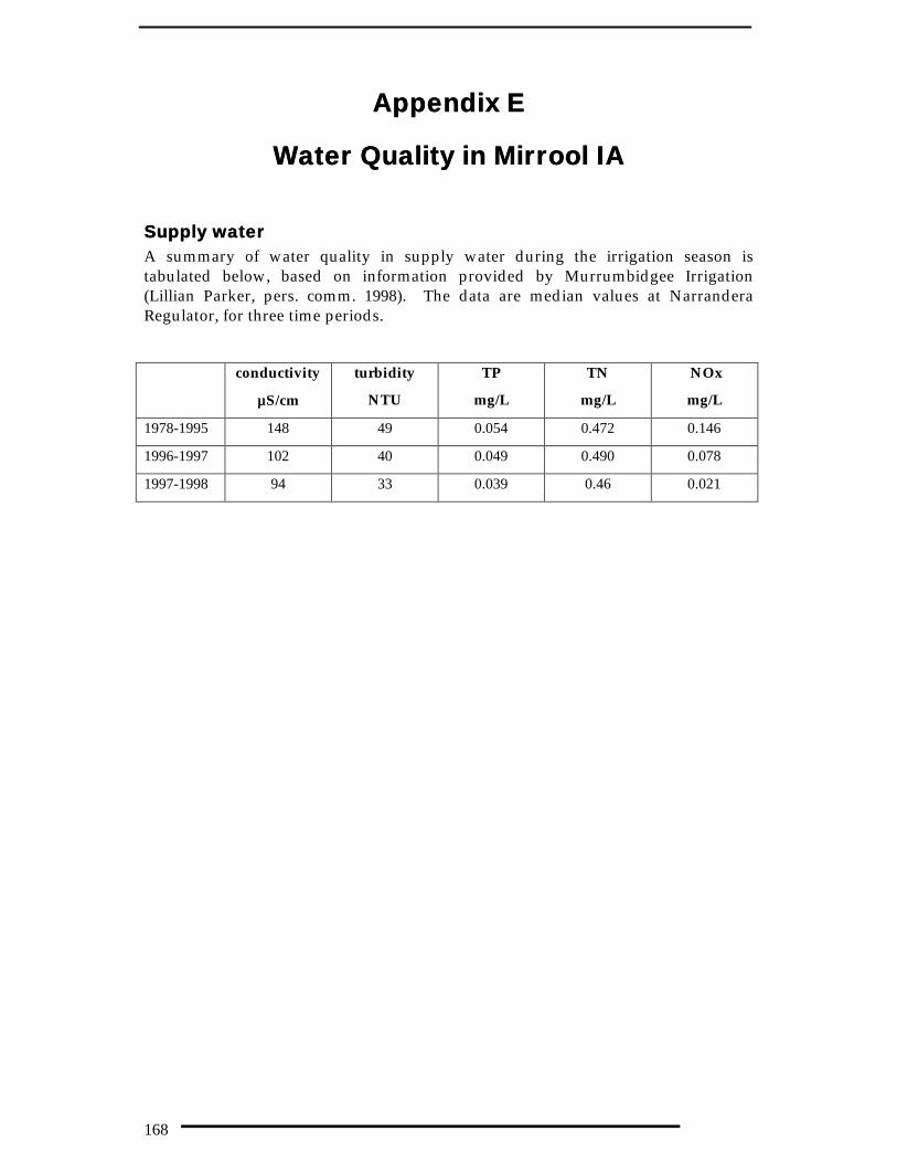
168
Appendix EAppendix E
Water Quality in Mirrool IAWater Quality in Mirrool IA
Supply waterSupply waterA summary of water quality in supply water during the irrigation season istabulated below, based on information provided by Murrumbidgee Irrigation(Lillian Parker, pers. comm. 1998). The data are median values at NarranderaRegulator, for three time periods.
conductivity
µµS/cm
turbidity
NTU
TP
mg/L
TN
mg/L
NOx
mg/L
1978-1995 148 49 0.054 0.472 0.146
1996-1997 102 40 0.049 0.490 0.078
1997-1998 94 33 0.039 0.46 0.021

169
Pesticides in MIA irrigation drainagePesticides in MIA irrigation drainage
The table below shows which pesticides have been detected in irrigation drainagefrom December to May, for four successive years. Note that this is simply presence,and not abundance of chemicals.
Month 1994-1995 1995-1996 1996-1997 1997-1998
December atrazine atrazine atrazine atrazinebromacil bromacil bromacildiuron diuron diuron diuron
endosulfan sulfateMCPA
metolachlor metolachlor metolachlor metolachlormolinate molinate molinate molinatesimazine simazine simazine
thiobencarbtotal endosulfan total endosulfan total endosulfan
January atrazine atrazine atrazinebromacil bromacil bromacildiuron diuron diuron
endosulfan sulfatemetolachlor metolachlor
molinate molinate molinate molinatesimazine simazinetotal edosulfan total endosulfan total endosulfan
February 2,4-D 2,4-Datrazine atrazine atrazinebromacil bromacil bromacil bromacildiuron diuron diuron
endosulfan sulfateMCPA MCPA
metolachlortotal endsulfan total endosulfan total endosulfan
March atrazinebromacil
diuron diuron diuronendosulfan sulfatemetolachlor
molinatetotal endosulfan total endosulfan total endosulfan
April atrazine atrazinediuron diuron diurontotal endosulfan total endosulfan
May atrazine atrazine atrazinebromacil bromacil bromacil
diuron diuron diuronsimazine simazine
total endosulfan total endosulfan