Embed Size (px)
Citation preview
The Role of Rheology in the Flow and Mixing of
Complex Fluids
by
Sara Ghorbanian Farah Abadi
A thesis submitted to
The University of Birmingham
for the degree of
MASTER OF PHILOSOPHY
School of Chemical Engineering
College of Engineering and Physical Sciences
The University of Birmingham
November 2016

University of Birmingham Research Archive
e-theses repository This unpublished thesis/dissertation is copyright of the author and/or third parties. The intellectual property rights of the author or third parties in respect of this work are as defined by The Copyright Designs and Patents Act 1988 or as modified by any successor legislation. Any use made of information contained in this thesis/dissertation must be in accordance with that legislation and must be properly acknowledged. Further distribution or reproduction in any format is prohibited without the permission of the copyright holder.
ABSTRACT
Mixing of fluids with complex rheology is encountered more and more frequently in
industries. Nonetheless, mixing behaviour of such fluids is still poorly understood due to
the complexity of their rheological behaviour. This study aims to enhance fundamental
understanding of the flow and mixing of rheologically complex fluids such as thixotropic,
shear-thinning and viscoelastic fluids. The objectives of this study were to investigate
within stirred vessels the effects of thixotropy and viscoelasticity, separately, in the
absence of other rheological behaviours for the fluids examined. To achieve these aims
the rheological behaviour of the fluid examined is isolated by using a fluid that exhibits
only one of these behaviours of interest at a time. The Particle Image Velocimetry (PIV)
technique was employed to characterize the flow fields of fluids. The flow pattern,
normalized mean velocity and cavern growth in the vessel were characterized during the
mixing for both thixotropic and viscoelastic fluids. The results were compared to the
reference fluids under laminar and transition regimes. Three different types of impeller
were investigated: Rushton turbine (RTD), and Pitch Blade Turbine (PBT) in up pumping
mode (PBTU) and in down pumping mode (PBTD). Additional work was conducted
using th Planar Laser Induced Fluorescence (PLIF) visualization technique to investigate
in more detail the evolution of mixing in a cavern with time for a thixotropic fluid. The
mixing efficiency of the impellers was analyzed in terms of impeller pumping efficiency
and size and growth of a cavern.

Dedicated To My Beloved Parents

ACKNOWLEDGEMENTS
Firstly, I would like to thank my supervisor Professor M. Barigou for his guidance during
the course of my research. I would like to express my gratitude towards Professor Mark
Simmons for valuable advice and support throughout this work.
I would like to thank the following people: Dr. Andreas Tsoligkas for his first training
with PIV experiments, and Dr. Federico Alberini for his guidance in using PIV and PLIF
techniques; Dr. Asja Portsch, Dr. Taghi Miri, and Dr. James Bowen for the introduction
and advice on using a Rheometer; Dr. Hamed Rowshandel for his valuable advice in
Matlab, and Dr. Halina Murasiewicz and Dr.Artur Majewski for their generous support
through this research.
In addition, I would like to express my appreciation, for their valuable help concerning
the experimental setup, to David Boylin, Thomas Eddleston and Steven Williams from
the workshop team.
I would also like to thank all the great people from the General Office, especially Lynn
Draper, for their friendship and continuous support. I want to thank Zainab Alsharify,
Shahad Al-Najjar Dr. Li Liu for their friendship and support.
I have to also thank the student services team, especially Julie Kendall and Laura Salkeld,
for their understanding and support.
Last but not least, I would like to thank my family: my beloved parents, lovely sister,
supportive brother, and sweet grandmother for their encouragement and infinite
understanding and support. I have to also thank my husband for his understanding and
supports.
TABLE OF CONTENTS
Chapter 1: INTRODUCTION ....................................................................................................... 1 1.1 Motivation................................................................................................................ 1 1.2 Objectives ................................................................................................................ 3 1.3 Thesis layout ............................................................................................................ 4
Chapter 2: LITERATURE REVIEW ............................................................................................ 5
2.1 Mixing Systems ....................................................................................................... 5 2.1.1 Mechanically Agitated Vessels .............................................................................. 6
2.1.2 Flow Regime .......................................................................................................... 7
2.1.2.1 Laminar and Transitional Flow Regimes .............................................. 9
2.1.2.2 Turbulent Regime................................................................................ 11
2.1.3 Impeller selection and resulting flow patterns ..................................................... 12
2.1.4 Unconventional Geometry ................................................................................... 18
2.1.5 Mixing Times ....................................................................................................... 19
2.2 Fluid Rheology ...................................................................................................... 21 2.1.1 Newtonian and non-Newtonian Fluids ................................................................. 21
2.2.1 Viscoelastic Fluid ................................................................................................. 23
2.2.2 Viscoplastic Fluid ................................................................................................ 26
2.1.2 Thixotropic Fluid ................................................................................................. 28
2.3 Visualization Techniques....................................................................................... 30 2.3.1 Hot Wire Anemometry (HWA) ........................................................................... 31
2.3.2 Laser Doppler Velocimetry/Anemometry (LDV/A) ............................................ 32
2.3.3 Planar laser Induced Fluorescence (PLIF) ........................................................... 34
2.3.4 Particle Image Velocimetry (PIV) ....................................................................... 35
2.3.5 Positron Emission Particle Tracking (PEPT) ....................................................... 37
Chapter 3: EXPERIMENTAL TECHNIQUE AND THEORETICAL ANALYSIS .................. 40
3.1 Apparatus ............................................................................................................... 40
3.2 Particle Image Velocimetry (PIV) ......................................................................... 43 3.3 Planar Laser Induced Fluorescence (PLIF) ........................................................... 45
3.4 Flow Number ......................................................................................................... 47
Chapter 4: EFFECT OF THIXOTROPY ON FLUID MIXING IN A STIRRED TANK .......... 50
4.1 Introduction............................................................................................................ 51 4.2 Material and Experimental Design ........................................................................ 53
4.2.1 Rheology of Test Fluids ....................................................................................... 53
4.2.1.1 Time Dependent Fluids (Thixotropy) ................................................. 53
4.2.1.2 Time Independent Fluids..................................................................... 54
4.2.2 Rheology Results ................................................................................................. 54
4.2.2.1 Hysteresis Loop Test ........................................................................... 56
4.2.2.2 Steady State Shear Viscosity ............................................................... 57
4.2.3 Experimental Design ............................................................................................ 61
4.2.4 Experimental Techniques ..................................................................................... 61
4.3 Results and Discussion .......................................................................................... 62 4.3.1 Flow Fields ........................................................................................................... 63
4.3.1.1 Re = 158 .............................................................................................. 63
4.3.1.2 Re = 61 ................................................................................................ 72
4.3.1.3 Re = 7 .................................................................................................. 72
4.3.2 Cavern Growth ..................................................................................................... 76
4.3.3 Effect of Non-standard Configurations ................................................................ 80
4.3.3.1 Un-baffled Vessel................................................................................ 80
4.3.3.2 Off-bottom Clearance Effects ............................................................. 89
4.4 Conclusions ........................................................................................................... 94
Chapter 5: THE EFFECT OF VISCOELASTICITY IN A STIRRED TANK ........................... 97
5.1 Introduction............................................................................................................ 97 5.2 Rheology and Material Characterization ............................................................. 100
5.2.1 Test fluids ........................................................................................................... 100
5.2.1.1 Viscoelastic Fluid (Boger Fluid) ....................................................... 100
5.2.1.2 Newtonian Fluid ................................................................................ 101
5.2.1.3 Shear-thinning Inelastic Fluid ........................................................... 101
5.2.2 Rheology of Test Fluids ..................................................................................... 102
5.3 Experimental Setup .............................................................................................. 108 5.4 Results and Discussion ........................................................................................ 108
5.4.1 Newtonian Fluid (N93, N95) ............................................................................. 109
5.4.1.1 Re = 80 .............................................................................................. 109
5.4.1.2 Re = 45 .............................................................................................. 113
5.4.1.3 Re = 7 ................................................................................................ 114
5.4.1.4 Shear-thinning Inelastic Fluid ........................................................... 115
5.4.2 Low viscoelastic Boger Fluids (100PAA) ......................................................... 116
5.4.2.1 RTD Configuration ........................................................................... 116
5.4.2.2 PBTU Configuration ......................................................................... 119
5.4.2.3 PBTD Configuration ......................................................................... 122
5.4.3 High viscoelastic Boger Fluid (300PAA) .......................................................... 123
5.4.4 Pseudo-Caverns .................................................................................................. 128
5.4.5 Conclusions ........................................................................................................ 129
Chapter 6: CONCLUSIONS AND FUTURE WORK.............................................................. 131
6.1 Conclusions ......................................................................................................... 131
6.2 Future work .......................................................................................................... 133 REFERENCES ................................................................................................................. 135
LIST OF FIGURES
Figure 2.1. Schematic representation of a typical mechanically agitated vessel (Edwards
et al., 1997) ........................................................................................................................ 7
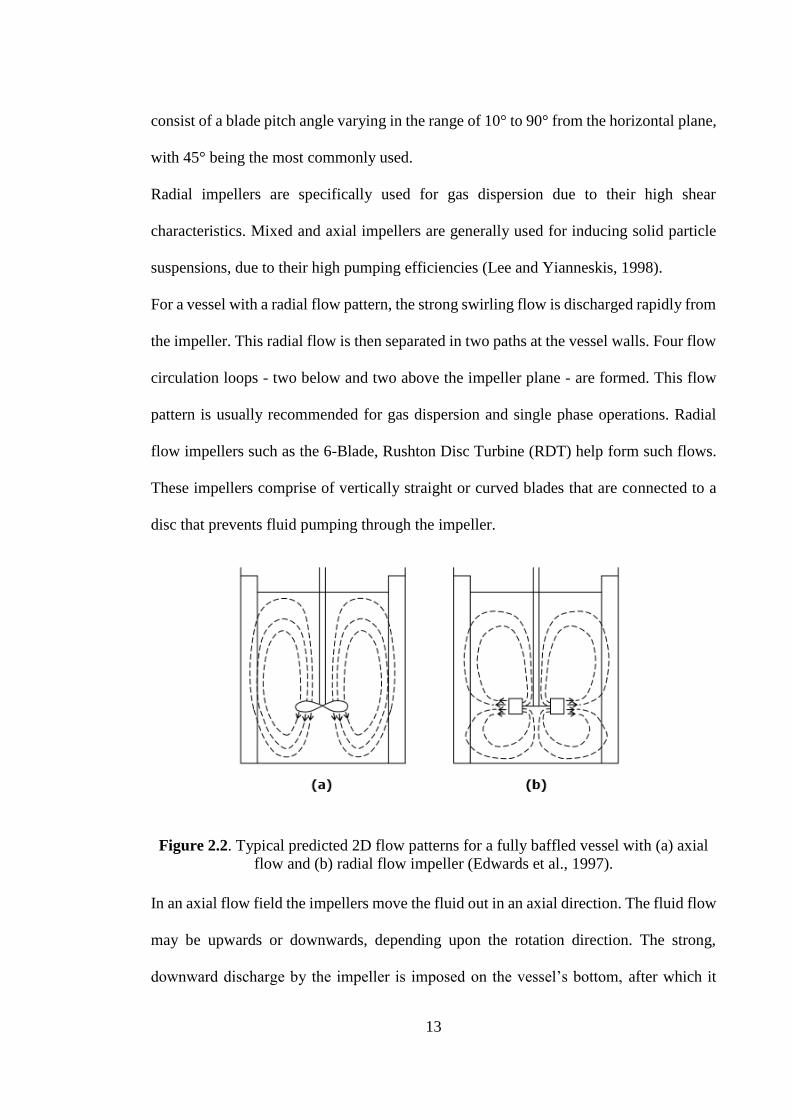
Figure 2.2. Typical predicted 2D flow patterns for a fully baffled vessel with (a) axial
flow and (b) radial flow impeller (Edwards et al., 1997). ............................................... 13
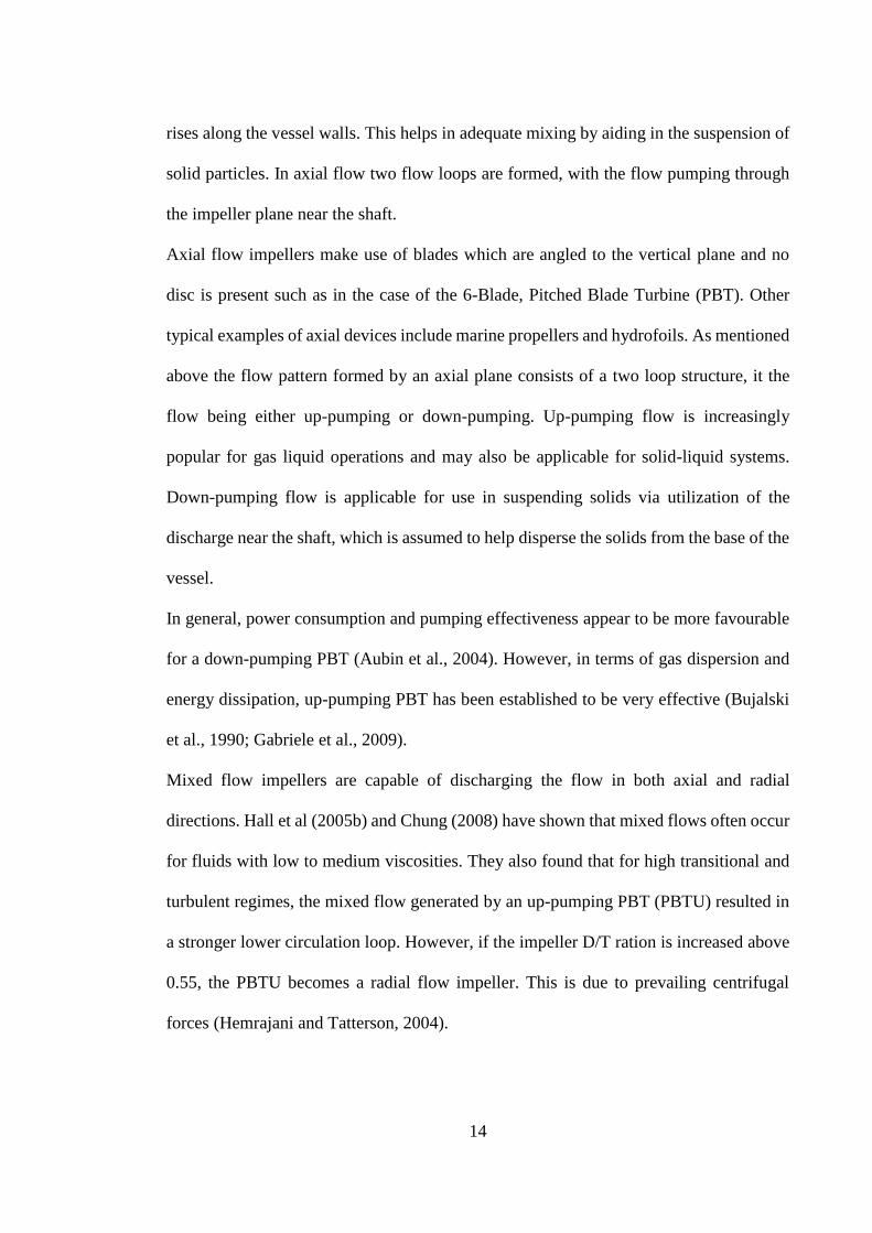
Figure 2.3. Schematic illustration of 2D flow patterns around a radial flow impeller in a
viscoelastic fluid, (a) low EI, (b) intermediate EI, (c) high EI (Özcan-Taskin and Nienow,
1995) ............................................................................................................................... 15
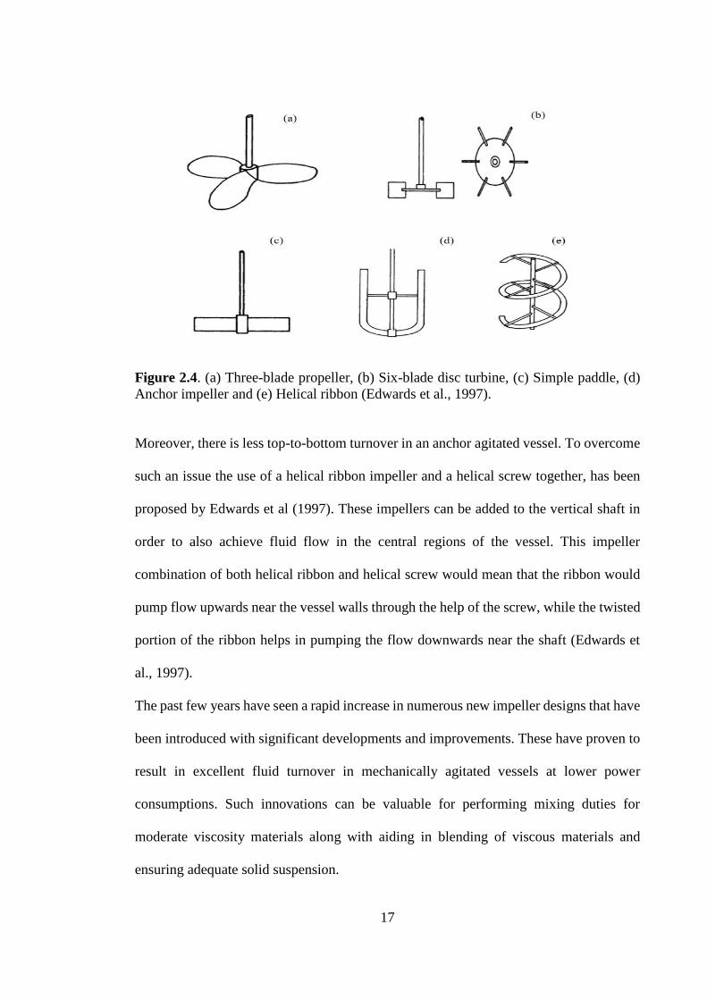
Figure 2.4. (a) Three-blade propeller, (b) Six-blade disc turbine, (c) Simple paddle, (d)
Anchor impeller and (e) Helical ribbon (Edwards et al., 1997). ..................................... 17
Figure 2.5. Mixing time measurement (Edwards et al., 1997) ....................................... 20
Figure 2.6. Rheological properties of Newtonian and non-Newtonian fluids (Paul et al.,
2004) ............................................................................................................................... 22
Figure 2.7. Stress components around a rotating coaxial cylinder (Özcan-Taskin, 1993)
......................................................................................................................................... 24
Figure 2.8. Breakdown of a 3D thixotropic structure (Barnes, 1997) ............................ 30
Figure 2.9. A typical LDV experimental set up, 1: laser; 2: fiber-optical module; 3:
transmitting/receiving optics; 4: stirred vessel; 5: photomultipliers; 6: flow velocity
analyser; 7: oscilloscope; 8: computer; 9: intersection of the two laser beams (Guida,
2010) ............................................................................................................................... 32
Figure 2.10. Simplified PLIF experimental facility. ...................................................... 35
Figure 2.11. Simplified, typical PIV set-up, Image taken from (Guida, 2010).............. 36
Figure 2.12. Schematic illustration of a PEPT experimental set-up showing positron
annihilation and 𝛾-ray detection by the PEPT camera, Image taken from (Guida, 2010)
......................................................................................................................................... 38
Figure 3.1. The layout of the stirred vessel configurations, equipped with impeller, as
used in this work. (a) baffled, (b) un-baffled. ................................................................. 41
Figure 3.2. Impeller geometries used in the experiments, a) PBT, b) RTD ................... 42
Figure 3.3. Schematic of various off-bottom clearance configurations studied in this work
......................................................................................................................................... 43
Figure 3.4. Experimental setup for PIV measurements ................................................. 44
Figure 3.5. Pixel greyscale versus tracer concentration ................................................. 46
Figure 3.6. Experiment setup for PLIF experiments ...................................................... 46
Figure 3.7. Schematic diagram of flow rates for PBTD impeller taken from (Guida et al.,
2010). .............................................................................................................................. 48
Figure 4.1. 2.2w% Laponite fluid under application of shearing followed by a
recoveryperiod for three different shear rates……………………………………….. 55
Figure 4.2. Viscosity curve overlap in test runs. ............................................................ 56
Figure 4.3. (a) Full shear ramp experiment of 2.2w% Laponite fluid (six ramps), ........ 58
Figure 4.4. Schematic of steady shear flow tests; (a) few constant shear stress applied to
the thixotropic fluid (b) response of shear rate at constant shear stress over a time of
experiments. .................................................................................................................... 59
Figure 4.5. Flow curves corresponding to different shearing times of 2.2w% Laponite.
......................................................................................................................................... 59
Figure 4.6. Flow curve of 1w% Carbopol fluid at different shearing times. .................. 60
Figure 4.7. The contour of normalized velocity magnitude of three impellers for 2.2w%
Laponite at Re = 158. ...................................................................................................... 65
Figure 4.8. Velocity vector on an axial-radial plane for a two flow regime at Re = 61 and
Re=158 for both fluids mixed by the PBTD impeller. .................................................... 66
Figure 4.9. The contour of normalized magnitude velocity for the three impellers at ... 68
Figure 4.10. Velocity vector on an axial-radial plane for two flow regimes Re = 61, Re
=158 for both fluids mixed with the PBTU impeller. ..................................................... 69
Figure 4.11. Contour of shear strain rate plot for 2.2w% Laponite (at t1 and t3) and 1w%
Carbopol fluid. ................................................................................................................ 71
Figure 4.12. The contour of normalized magnitude velocity for three impellers for
2.2w% Laponite at Re = 61. ............................................................................................ 73
Figure 4.13. (a) Normalized magnitude velocity for three impellers at Re= 7 for 2.2w%
Laponite fluid at t3, (b) velocity field for three impellers at Re = 7 for 2.2w% Laponite
fluid at t3. ......................................................................................................................... 75
Figure 4.14. The changes of normalized cavern area % for the thixotropic fluid as a
function of time for (a) Re= 158 and (b) Re = 61. .......................................................... 76
Figure 4.15. The cavern height and radius growth as a function of time for the thixotropic
fluid at (a) Re =158, (b) Re = 61. .................................................................................... 77
Figure 4.16. Schematic diagram of cavern growth while mixing for 2.2w% Laponite and
1w% Carbopol at Re = 61. .............................................................................................. 78
Figure 4.17. The cavern growth from PLIF experiments for both 1w% Carbopol and
2.2w% Laponite fluid at Re = 7. ...................................................................................... 79
Figure 4.18. Variation of Power number as a function of Reynold number for viscoplastic
fluid in the (a) baffled vessel and (b) un-baffled vessel. Image adopted from Hirata and
Aoshima (1996). .............................................................................................................. 81
Figure 4.19. The cavern shape and size for the thixotropic and viscoplastic fluids in the
baffled and un-baffled vessel at Re = 158. ...................................................................... 82
Figure 4.20. The contour of normalized magnitude velocity of three impellers at Re = 61
for 1 w% Carbopol. ......................................................................................................... 84
Figure 4.21. The Normalized mean velocity component (radial and axial) at two axial
positions for 1w% Carbopol and 2.2w% Laponite at Re =158 in a baffled and un-baffled
tank. ................................................................................................................................. 85
Figure 4.22. The normalized mean velocity component (radial and axial) at three
horizontal positions for 1w% Carbopol and 2.2w% Laponite at Re = 158 in a baffled and
un-baffled tank. ............................................................................................................... 86
Figure 4.23. The cavern size growth ratio for the thixotropic fluid during mixing in the
baffled and un-baffled vessel at Re =158. ....................................................................... 87
Figure 4.24. The contour of normalized magnitude velocity for three impellers at ...... 88
Figure 4.25. The contour of normalized velocity magnitude plot of 2.2w% Laponite at t3
and 1w% Carbopol for the PBTD impeller at Re = 158 and for four off bottom impeller
clearances. ....................................................................................................................... 91
Figure 4.26. The contour of normalized magnitude velocity plot of 2.2w% Laponite at
t3 and 1w% Carbopol for the PBTU impeller at Re=158 and for four off bottom impeller
clearances. ....................................................................................................................... 92
Figure 4.27. The cavern size growth ratio for 2.2w% Laponite as a function of time for
four impeller clearance positions. ................................................................................... 93
Figure 5.1. Steady shear properties for all tests fluids a), viscosity versus shear rate and
b) shear stress versus shear rate. ................................................................................... 104
Figure 5.2. First normal stress difference N1 (Pa) of viscoelastic fluids as a function of
shear rate (s-1) ................................................................................................................ 106
Figure 5.3. The contour of normalized velocity magnitude of three impellers for the
Newtonian fluid N93, at three flow regimes: Re = 80, Re = 45, Re = 7 ....................... 111
Figure 5.4. The contour of normalized velocity magnitude of three impellers for the
Newtonian fluid N95, at three flow regimes: Re = 80, Re = 45, Re = 7. ...................... 112
Figure 5.5. The contour of normalized velocity magnitude of three impellers for the
shear-thinning fluid 1.5w% CMC, at three flow regimes: Re = 80, Re = 45, Re = 7. ... 117
Figure 5.6. a)The contour of normalized velocity magnitude and b) the streamline plots
of the viscoelastic Boger fluid 100PAA for three impeller types at Re = 80. ............... 118
Figure 5.7. Flow pattern observation for the RDT impeller in a baffled vessel: (a) low
(El), (b) intermediate (El) and appearance of secondary reverse flow (1), (c) high (El).
....................................................................................................................................... 119
Figure 5.8. Flow pattern observation for the PBTU impeller in a baffled vessel a)
Newtonian fluid b) viscoelastic fluid with high (El), c) viscoelastic fluid with intermediate
(El) : Note the reverse flow field in (1), the appearance of secondary counter-rotating ring
vortex in (2), and the secondary reverse flow in (3). ................................................... 120
Figure 5.9. a) The contour of normalized velocity magnitude and b) the streamline plot
of three impellers for the viscoelastic Boger fluid 100PAA at Re = 45. ....................... 121
Figure 5.10. Flow pattern observation for the PBTD impeller in a baffled vessel:
a) Newtonian fluid, b) viscoelastic fluid with low (El), c) viscoelastic fluid with
intermediate (El), d) viscoelastic fluid with high (El); Note the reverse flow field in (1),
the appearance of a secondary counter-rotating ring vortex in (2) and the growth of a
secondary ring vortex in (3) .......................................................................................... 122
Figure 5.11. a)The contour of normalized velocity magnitude and b) the streamline plot
of the three impellers for the viscoelastic Boger fluid 100PAA at Re = 7 .................... 124
Figure 5.12. The Contour of normalized velocity magnitude of three impellers for the
300PAA Boger fluid, at three flow regimes: Re = 80, Re = 45, Re = 7. ....................... 125
Figure 5.13. The streamline plots for all test fluids used in this study at Re = 80 under
three impeller configurations. ....................................................................................... 126
Figure 5.14. The streamline plots for all test fluids used in this study at Re = 45 under
three impeller configurations. ....................................................................................... 127
Figure 5.15. Pseudo-cavern boundaries for different impellers at three flow regimes: Re
= 7, Re = 45, and Re = 80. ............................................................................................. 129
LIST OF TABLES
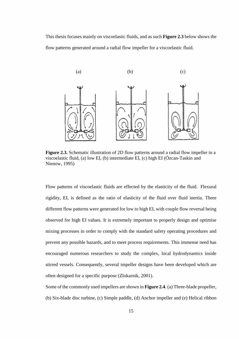
Table 2.1: Viscosity and speed relationship with impeller type. .................................... 16
Table 3.1. Dimensions of impellers used in experiments ............................................... 42
Table 4.1. Rheology parameter of Herschel–Bulkley model for different shearing times
during experiment 2.2w% Laponite fluid ....................................................................... 60
Table 4.2. Different configurations used in this study; B: baffled vessel, U: un-baffled
vessel ............................................................................................................................... 61
Table 4.3. Characterized parameters of flow for the PBTD impeller. ............................ 64
Table 4.4. Characterized parameters of flow for PBTU impeller. .................................. 67
Table 4.5.Characterized parameter of flow for RTD impeller. ....................................... 67
Table 4.6. Characterized parameters of flow for thixotropic fluid in the un-baffled vessel.
......................................................................................................................................... 82
Table 5.1: Composition and density of test fluids used ................................................ 101
Table 5.2: Rheological properties of fluids used in the experiments. ........................... 105
Table 5.3: Dimensionless numbers over the range of impeller speed for the viscoelastic
fluids used in the experiments. ...................................................................................... 107
Table 5.4: All experimental configurations and setup used in this study. .................... 108
Table 5.5. Characteristic parameters of flow for the Newtonian fluid N93. ................. 110
Table 5.6. Characteristic parameters of flow for the Newtonian fluid N95. ................. 113
Table 5.7. Characterized parameter of flow for shear-thinning fluid 1.5w% CMC. ..... 115
Table 5.8. Ratio of pseudo-cavern area to tank area (AC/AT) % for the test fluids N93 and
100PAA ......................................................................................................................... 128
1 NOMENCLATURE
D Impeller diameter
m
H Vessel fill height m
B width of wall baffles m
C Off-bottom clearance m
T Diameter of vessel m
N
M
Impeller rotational speed
Image magnification
s-1
μm /pixel
Q Impeller pumping rate m3 s-1
Qa Axial impeller pumping rate m3 s-1
Qr
L
𝐿𝐼𝐴
Radial pumping rate
characteristic length
The length of the integration area
m3 s-1
m
m
r Radial distance m
z Axial distance
m
𝑘𝑠 Metzner and Otto constant -
k Consistency index Pa sn
n Flow behavior index -
N1 First normal stress difference Pa
N2
Second normal stress difference Pa
A Constant value
-
b Constant value
-
u tip Impeller tip velocity m s-1
urz mean radial axial velocity m s-1
u The radial velocity component m s-1
v The axial velocity component m s-1
AC Cavern area m2
AT Tank area m2
t Time s
df Fringe spacing M
fD Doppler frequency Hz
v Kinematic viscosity m2 s-1
Greek symbols
µ Viscosity Pa s
μa Apparent Viscosity Pa s
ηB Plastic viscosity Pa s
ρ Density kgm-3
τ Shear Stress, N/m2 Pa
γ
𝜏𝑦
Shear rate
Fluid yield stress
s-1
Pa
x y z Cartesian coordinates m
λ Wavelength m
ϑ Azimuthal coordinate rad
ѱ Normal stress difference coefficient Pa s2
Ø Angle °
Dimensionless Numbers
Re Reynolds number
Reimp
𝑅𝑒𝑃𝐿
Impeller Reynolds number
Reynold number/ Power low model
𝑅𝑒𝐻𝐵
El
Reynold number/Herschel-Bulkley
Elasticity number
Wi Weissenberg number
Fl Flow number
Abbreviations
PBT Pitched blade turbine
PBTD Down-pumping PBT
PBTU Up-pumping PBT
RTD Ruston disc turbine
PEPT Positron emission particle tracking
PIV Particle image velocimetry
PLIF Planar laser induced fluorescence
LDV Laser Doppler velocimetry
1
Chapter 1
INTRODUCTION
1.1 Motivation
The mixing of fluids in stirred vessels is by far one of the most common processes
encountered throughout the industry in many different processes. Correct mixing is
needed to ensure homogeneity of materials so as to achieve the desired product.
Improving mixing efficiency plays a major role in attaining high-quality product in the
industry.
Mixing of fluids with complex rheology is being incorporated more and more frequently
in various industrial processes, such as in fermentation, pharmaceuticals, polymerization,
personal and home care products and food products. However, an understanding of the
mixing behaviour of such fluids is lacking (Collias and Prud'homme, 1985). The
rheological complexities of non-Newtonian fluids can cause a plethora of difficulties in
mixing. Shear-thinning liquids, for example, display different behaviour compared to
Newtonian liquids during mixing, as increase in shear rate leads to significant decrease
in viscosity. In addtion, for shear-thinning liquids different viscosities can be observed in
various parts of the mixing vessel, so it is hard to set up the right operating conditions and
equipment to maximize the mixing efficiency. The exact opposite behaviour is displayed
by shear thickening fluids; the viscosity will be higher once the shear rate is increased.
During the mixing of non-Newtonian fluids with a yield stress a cavern is formed, which
is the region around the impeller where shear stresses are high.and hence the fluid is
mobile. Oustside the cavern, in area away from impeller, shear stresses are small and as
2
such the liquid is stagnant. A pseudo-cavern can be observed in the case of mixing shear-
thinning fluids or highly viscous Newtonian fluids. In the case of the pseudo-cavern the
fluid beyond the cavern boundaries is in motion, however the velocities are small. An
extensive investigation into the formation of caverns and pseudo-caverns developed
during mixing of non-Newtonian fluids was done by Adams and Barigou (2007).
Furthermore, Thixotropy is one of the challenging rheological phenomena in non-
Newtonian fluid science. Thixotropic fluids have extensive applications in natural
systems but also in industry, with mixing of such fluids being widely used in the food,
polymer and pharmaceutical industries. Nonetheless, thixotropy is still poorly understood
due to the complexity of the microstructure of thixotropic fluids. Such fluids show a
decrease in viscosity over time for a continuously applied shear stress, often with yield
stress. Mixing of complex fluids with shear-thinning time dependency and yield stress is
challenged in the mixing industry.
The mixing of viscoelastic fluids is commonly carried out in stirred tanks in many
industrial processes. Viscoelastic fluids show varying flow patterns under different
mixing conditions, often climbing the rotating shaft due to normal forces, and also
affecting the power drawn (Collias and Prud'homme, 1985). Such fluids display other
complex rheological properties, for example shear thinning behaviour. This behavior has
been studied in the literature extensively however, the effect of viscoelasticity in a stirred
vessel has not been properly addressed, due to the difficulty encountered in separating the
effects of viscoelasticity from other rheological properties, and as such it is still poorly
understood.
3
As such the motivation for this work came from the need for a better understanding of the
role of non-Newtonian fluid behavior, especially thixotropy and viscoelasticity on fluid
mixing in a stirred vessel.
1.2 Objectives
The objectives of this study are:
This project aims to enhance fundamental understanding of a number of issues
concerned with the flow and mixing of rheologically complex fluids, in particular
the impact of different rheological behaviors on the fluid dynamics and mixing in
stirred vessels.
Ordinary fluids exhibit a combination of rheological behaviors, e.g. shear-
thinning, elasticity, yield stress, thixotropy etc. The aim of this project is to try
and isolate rheological behaviors one at a time by using model fluids that exhibit
only one of these behaviors each time. As such, the effects of each rheological
behavior can be separately studied and identified. Boger Fluid, one of the
formulated fluids of this study, was used to investigate the effect of viscoelasticity
in a stirred tank for it exhibits viscoelasticity in the absence of other complex
rheological behaviors.
Transparent, formulated fluids underwent classic characterization techniques
such as rheology, and also new flow visualization techniques such as Particle
Image Velocimetry (PIV) and Planar Laser Induced Fluorescence (PLIF) so as to
improved scientific understanding of mixing of complex fluids in a stirred vessel.
4
1.3 Thesis layout
Following the current Introduction Chapter is a comprehensive review of existing
literature on different aspects of single-phase fluid mixing in stirred tanks, an introduction
to fluid rheology and non-Newtonian fluid behavior and a review of the existing flow
visualization techniques, as presented in Chapter 2. The experimental procedures,
experimental techniques and equipment used, and the theory for analysis of PIV data are
given in Chapter 3.
Chapters 4 and 5 are results chapters. Details of materials, fluid rheology results and the
experimental procedures are given in each of these chapters. Chapter 4 presents results
regarding the effect of thixotropy on fluid mixing. Results for a thixotropic fluid are
obtained from PIV and PLIF techniques and are discussed and compared with those of a
time-independent fluid. A full study of thixotropic rheology is presented in this chapter.
In addition, viscoplastic fluid behavior is similarly investigated. Subsequently, Chapter 5
explores the mixing of a viscoelastic fluid via use of PIV. The behaviour of a viscoelastic
fluid during mixing is compared with that of a shear-thinning fluid and a Newtonian fluid.
Please note that the test fluids rheology and results are discussed separately in each results
chapter, in order to clarify ideology of fluid rheology behavior used in each chapter.
Finally, the conclusions from this work and suggestions for future work are presented in
Chapter 6.
Notation and References sections that are used in each chapter have been grouped and are
presented at the end of the thesis.
5
2 Chapter 2
LITERATURE REVIEW
Mixing operations are one of the most commonly employed processes in several
industries, such as the pharmaceuticals, chemicals, food processing and mineral. In such
industrial settings fluid mixing can take place in a range of different types of equipment.
These include in-line static mixers, rotor-stator mixers and mechanically agitated vessels.
Amongst the wide variety of mixers, mechanically agitated vessels have been considered
to be the most commonly used mixing devices. The goal is to achieve a desired process
result for the fluid mixed system, and ensure reduction of inhomogeneity and non-
uniformity in the system. The process fluid used in mixing operations may exist either in
a single phase or in multiple phases. Understanding mixing of complex fluids may be
very tedious, as their complex rheological behaviour makes it very difficult to understand
the results of their mixing studies. In addition, not much work has been done to understand
the mixing behaviour of such fluids. This chapter provides a general description of the
mixing phenomena along with describing flow regimes, flow patterns and several
geometrical parameters. This review also focuses on the different fluid rheologies of non-
Newtonian fluids, namely viscoelastic, shear-thinning and thixotropic fluids. Finally, a
critical analysis of the different experimental techniques relevant to this work is provided.
2.1 Mixing Systems
Mixing is commonly defined as the reduction of inhomogeneity in order to achieve a
desired process result. It plays a key role in a range of industries varying from fine
chemicals and petrochemicals to food and biotechnology (Paul et al., 2004). Mixing
6
operations are generally classed depending upon the type of process materials. Examples
of some commonly used process materials include viscous liquids, solid-liquid and gas-
liquid systems. Based on the extensive research done within the field of chemical
engineering, it is certain that the solid-liquid mixing process is the most commonly used
and as such the most important one.
An enormous range of mixing equipment is currently commercially available, indicating
to the wide range of mixing requirements typically needed in the chemical processing
industry. To perform chemical mixing operations, numerous distinct types of mixers have
been utilized. However, the most commonly reviewed mixers are the mechanically
agitated vessels (Edwards et al., 1997).
2.1.1 Mechanically Agitated Vessels
Mechanically agitated vessels are the most common mixing equipment used in the
chemical, pharmaceutical and pulp and paper industries. More than 50% of the world’s
chemical processes involve the use of mechanically agitated vessels for the production of
high added value products (Paul et al., 2004). These vessels are used in the processing
industry for blending miscible liquids, achieving gas dispersion or solid suspension in a
liquid, and for carrying out efficient optimization of chemical reactions.
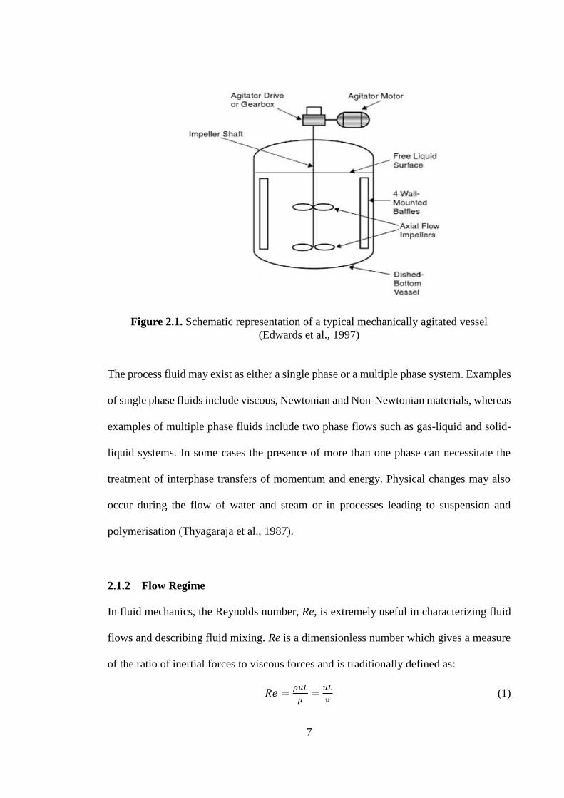
Figure 2.1 below is a simplified schematic representation of a typical mechanically
agitated vessel. This figure serves to demonstrate the overall configuration and the main
features of a baffled vessel, comprising of four baffles, a centrally located impeller shaft
and an impeller. Energy transfer from the rotating impeller to the process fluid promotes
fluid motion.
7
Figure 2.1. Schematic representation of a typical mechanically agitated vessel
(Edwards et al., 1997)
The process fluid may exist as either a single phase or a multiple phase system. Examples
of single phase fluids include viscous, Newtonian and Non-Newtonian materials, whereas
examples of multiple phase fluids include two phase flows such as gas-liquid and solid-
liquid systems. In some cases the presence of more than one phase can necessitate the
treatment of interphase transfers of momentum and energy. Physical changes may also
occur during the flow of water and steam or in processes leading to suspension and
polymerisation (Thyagaraja et al., 1987).
2.1.2 Flow Regime
In fluid mechanics, the Reynolds number, Re, is extremely useful in characterizing fluid
flows and describing fluid mixing. Re is a dimensionless number which gives a measure
of the ratio of inertial forces to viscous forces and is traditionally defined as:
𝑅𝑒 =𝜌𝑢𝐿
𝜇=
𝑢𝐿
𝑣 (1)
8
where 𝑢 is the mean fluid velocity.
For mixing studies in stirred vessels, the impeller Reynolds number is denoted as 𝑅𝑒𝑖𝑚𝑝
and is defined as:
𝑅𝑒𝑖𝑚𝑝 =𝜌𝑁𝐷2
𝜇 (2)
The impeller Reynolds number is generally useful in characterising different flow
regimes in mechanically agitated vessels. When 𝑅𝑒𝑖𝑚𝑝 < 10 the fluid flow is in laminar
regime, whereas when 𝑅𝑒𝑖𝑚𝑝 > 104 the fluid flow is in turbulent regime. The transitional
region lies between 10 to104 Reimp. It is feasible and quite useful to describe mixing
mechanisms under laminar or turbulent flow conditions, as they have evident differences
(Edwards et al., 1997).
As Non-Newtonian fluids shear-thinning materials by definition do not have a constant
viscosity, with their viscosity dropping as shear rate is increased. To represent the
rheological behaviour of these non-Newtonian materials, the best approach is to use the
power law model, shown below:
𝜏 = 𝑘��𝑛 (3)
The consistency factor provides a measure of fluid thickness while the flow behaviour
index measures the strength of non-Newtonian fluid. The value of the flow behaviour
index, n, for shear-thinning fluids lies between 0 and 1, being 1 for Newtonian fluids.
Equation 3 cannot be used to describe non-Newtonian fluids as the viscosity of these
materials is not constant. Therefore, the Metzner and Otto correlation needs to be applied
in order to calculate the average shear rate which, in turn, can help in calculating the
Reynolds number by the power law model as shown below:
9
𝑅𝑒𝑃𝐿 =𝜌𝑁2−𝑛𝐷2
𝑘𝑘𝑠𝑛−1 (4)
where ks is the Metzner and Otto constant, and its value is dependent on the impeller type.
For example, for a pitched blade turbine the ks value is between 11 and 13 (Metzner and
Otto, 1957).
Another type of non-Newtonian behaviour is shown by shear thickening materials, which
behave in the opposite manner to shear-thinning fluids in that for shear thickening
materials the viscosity increases with increase in the shear rate. Their rheological
behaviour can also be represented by the power law model (Equation. 3), whereby the
flow behaviour index being above unity. This is further discussed in section 2.2.3.
2.1.2.1 Laminar and Transitional Flow Regimes
Laminar regimes are mainly associated with high viscosity fluids. For a flow to be
completely laminar at typical rates of energy input, the value of viscosity must be large
enough to result in impeller Reynolds number less than 10. However, for fluids with such
high viscosity values, the fluid rheology is often very complex.
Laminar or transitional regimes usually predominate in cases where efficient mixing of
high viscosity fluids is difficult to achieve. Examples of such high viscosity fluids include
pastes, creams and paints. Inertial forces reduce due to the action of high viscosities in
laminar conditions. Therefore, to achieve adequate bulk motion, it is important for the
rotating impellers to occupy a significant area of the vessel (Edwards et al., 1997). Large
velocity gradients exist in the vicinity of these rotating impellers. These are known as
laminar regions, with high shear rates capable of deforming and stretching fluid elements.
Specifically, upon continuous shearing these fluid elements are thinned, elongated and
10
folded. Such mixing features are of high importance for mixing mechanisms in laminar
flow regimes (Edwards et al., 1997; Alvarez et al., 2002; Zalc et al., 2001).
Non-Newtonian fluids are mainly high viscosity fluids and their complex fluid rheology
causes their mixing features to be even more complicated. Such complications can arise
from the fluid’s viscosity dependence on shear time or its time dependent behaviour.
The power number, Po is a dimensionless variable that has been widely used as a function
of the Reynolds number, Reimp, to evaluate mixing operations. The relationship between
the two can be illustrated through a Po vs. Reimp curve. Metzner et al (1961) discusses that
for various types of impellers, the slope of this curve is found to be -1 in the laminar
regime, however in the transitional regime Po and Reimp have been found to have a
complex relationship (Galindo and Nienow, 1992; Brito-de la Fuente et al., 1997; Aubin
et al., 2000; Paul et al., 2004).
To summarise the above, it is evident that fluid mixing in stirred vessels possesses
considerable complexity irrespective of flow regime. Fluid rheology has a major
consequence on the flow patterns and mixing performances. As such, a good
understanding of the rheological properties of all types of fluids can help in fluid mixing
studies.
11
2.1.2.2 Turbulent Regime
In mixing vessels, fluid flow is classified as turbulent when the impeller Reynolds number
should be higher than 104. The inertial force imparted by the rotating impeller is sufficient
enough to circulate the fluid quickly throughout the vessel and back to the impeller again.
In addition, during this circulation turbulent eddy diffusion takes place, leading to
adequate mixing which is much more enhanced than mixing rates in laminar flows. In
turbulent flow, numerous eddies of different length scales and intensities exist. The
provoked motion of these turbulent eddies help in enhancing fluid mixing rates hence
making the turbulent regime a desirable regime for efficient mixing in stirred vessels
(Yianneskis et al, 1987). In laminar and transitional regions, lack of turbulent eddy
dissipation causes less efficient mixing.
Wu and Patterson (1989) performed a study on mixing characteristics of viscous fluids
and reported that the turbulence field in the turbulent regime exhibits three dimensional
velocity fluctuations. Escudie and Line (2006) further explain the presence of anisotropic
turbulence dissipations and periodic hydrodynamics exhibited by fluids under turbulent
regimes. The strongest turbulent intensity is found close to the impeller as compared to
other regions in a typical stirred vessel. Also, a large percentage of energy is dissipated
close to the impeller region (Cutter, 1966), whereas fluctuations in turbulent trailing
vortices are found behind the impeller blades (Yianneskis et al., 1987; Schäfer et al.,
1998; Escudié et al., 2004).
The power number, Po, is found to be independent of the Reynolds number, Reimp, in the
turbulent regime (Metzner et al., 1961; Galindo and Nienow, 1992; Brito-de la Fuente et
al., 1997; Aubin et al., 2000; Paul et al., 2004).
12
2.1.3 Impeller selection and resulting flow patterns
Flow patterns have been commonly studied as they characterize how well the system is
mixed. In order to better understand the fluid mixing configuration, it is important to study
and analyse the formation, shape and velocities of flow patterns. Literature reviews show
that most of the work done has been performed on Newtonian fluids. This is because most
non-Newtonian fluids are opaque and the commonly used visualisation techniques are
optical, thus requiring transparent materials. In addition, as mentioned earlier, non-
Newtonian materials have complex rheological properties (Maingonnat et al 2005).
As has been repeatedly reported in literature, flow patterns are highly dependent upon the
type of impeller used in stirred vessels. Flow patterns help determine the existence of
‘dead zones’ in the vessel or whether all particles are suspended in the liquid. The two
typical primary flow patterns that are formed in a baffled vessel with the standard
configuration for a Newtonian fluid in the turbulent region are shown in Figure 2.2. An
axial flow pattern for a propeller is shown in Figure 2.2a, while Figure 2.2b shows a
radial flow pattern for a disc turbine. It is obvious that the velocities at any particular
point will be unsteady and will show three dimensional characteristics (Edwards et al.,
1997).
Presently, a wide range of impellers are used industrially, which can be simply
categorised into three groups for use in a stirred vessel: radial impellers such as the
Rushton Disc Turbine (RDT), axial impellers such as the marine propeller (MP) and
mixed impellers such as the Pitched Blade Turbine (PBT). Briefly, RDT impellers
discharge fluid radially towards the vessel walls, MP impellers discharge the fluid axially,
upwards or downwards depending upon the direction of rotation and PBT impellers
13
consist of a blade pitch angle varying in the range of 10° to 90° from the horizontal plane,
with 45° being the most commonly used.
Radial impellers are specifically used for gas dispersion due to their high shear
characteristics. Mixed and axial impellers are generally used for inducing solid particle
suspensions, due to their high pumping efficiencies (Lee and Yianneskis, 1998).
For a vessel with a radial flow pattern, the strong swirling flow is discharged rapidly from
the impeller. This radial flow is then separated in two paths at the vessel walls. Four flow
circulation loops - two below and two above the impeller plane - are formed. This flow
pattern is usually recommended for gas dispersion and single phase operations. Radial
flow impellers such as the 6-Blade, Rushton Disc Turbine (RDT) help form such flows.
These impellers comprise of vertically straight or curved blades that are connected to a
disc that prevents fluid pumping through the impeller.
Figure 2.2. Typical predicted 2D flow patterns for a fully baffled vessel with (a) axial
flow and (b) radial flow impeller (Edwards et al., 1997).
In an axial flow field the impellers move the fluid out in an axial direction. The fluid flow
may be upwards or downwards, depending upon the rotation direction. The strong,
downward discharge by the impeller is imposed on the vessel’s bottom, after which it
14
rises along the vessel walls. This helps in adequate mixing by aiding in the suspension of
solid particles. In axial flow two flow loops are formed, with the flow pumping through
the impeller plane near the shaft.
Axial flow impellers make use of blades which are angled to the vertical plane and no
disc is present such as in the case of the 6-Blade, Pitched Blade Turbine (PBT). Other
typical examples of axial devices include marine propellers and hydrofoils. As mentioned
above the flow pattern formed by an axial plane consists of a two loop structure, it the
flow being either up-pumping or down-pumping. Up-pumping flow is increasingly
popular for gas liquid operations and may also be applicable for solid-liquid systems.
Down-pumping flow is applicable for use in suspending solids via utilization of the
discharge near the shaft, which is assumed to help disperse the solids from the base of the
vessel.
In general, power consumption and pumping effectiveness appear to be more favourable
for a down-pumping PBT (Aubin et al., 2004). However, in terms of gas dispersion and
energy dissipation, up-pumping PBT has been established to be very effective (Bujalski
et al., 1990; Gabriele et al., 2009).
Mixed flow impellers are capable of discharging the flow in both axial and radial
directions. Hall et al (2005b) and Chung (2008) have shown that mixed flows often occur
for fluids with low to medium viscosities. They also found that for high transitional and
turbulent regimes, the mixed flow generated by an up-pumping PBT (PBTU) resulted in
a stronger lower circulation loop. However, if the impeller D/T ration is increased above
0.55, the PBTU becomes a radial flow impeller. This is due to prevailing centrifugal
forces (Hemrajani and Tatterson, 2004).
15
This thesis focuses mainly on viscoelastic fluids, and as such Figure 2.3 below shows the
flow patterns generated around a radial flow impeller for a viscoelastic fluid.
Figure 2.3. Schematic illustration of 2D flow patterns around a radial flow impeller in a
viscoelastic fluid, (a) low EI, (b) intermediate EI, (c) high EI (Özcan-Taskin and
Nienow, 1995)
Flow patterns of viscoelastic fluids are effected by the elasticity of the fluid. Flexural
rigidity, EI, is defined as the ratio of elasticity of the fluid over fluid inertia. Three
different flow patterns were generated for low to high EI, with couple flow reversal being
observed for high EI values. It is extremely important to properly design and optimise
mixing processes in order to comply with the standard safety operating procedures and
prevent any possible hazards, and to meet process requirements. This immense need has
encouraged numerous researchers to study the complex, local hydrodynamics inside
stirred vessels. Consequently, several impeller designs have been developed which are
often designed for a specific purpose (Zlokarnik, 2001).
Some of the commonly used impellers are shown in Figure 2.4. (a) Three-blade propeller,
(b) Six-blade disc turbine, (c) Simple paddle, (d) Anchor impeller and (e) Helical ribbon
(a) (b) (c)
16
(Edwards et al., 1997).These are propellers, turbines, paddles, anchors, helical ribbons
and screws. These impellers are usually attached to a central vertical shaft located inside
a cylindrical vessel. The range of applications of each of these impellers depends greatly
upon the fluid viscosity in the stirred vessel. Table 2.1 below summarizes the capacity of
these different types of impeller. It can be seen that propellers, turbines and paddles are
usually used in operations concerning the mixing of low viscosity fluids while operating
at high rotational speeds (Edwards et al., 1997).
Other types of impellers, such as anchors, helical ribbon and helical screw are strong
enough to be generally used for laminar mixing of very viscous materials. They can sweep
the entire volume of the vessel and therefore operate at much slower speeds, depending
upon their size and power consumption.
Peters and Smith (1962) have performed an in-depth study on the viscous flow in an
anchor agitated vessel. Their study has shown that an anchor impeller is capable of
promoting rapid fluid motion near the vessels walls but is unable to induce any motion
near the shaft. Therefore, the liquid in the area near the shaft may be relatively stagnant.
Table 2.1.Viscosity and speed relationship with impeller type (Edwards et al., 1997)
Impeller Viscosity
•
•
• Viscosity increases
Propeller < 2kg/ms
Turbine < 50 kg/ms
Paddle < 1000 kg/ms
Anchor -
Helical ribbon -
Helical screw -
Speed increases
17
Figure 2.4. (a) Three-blade propeller, (b) Six-blade disc turbine, (c) Simple paddle, (d)
Anchor impeller and (e) Helical ribbon (Edwards et al., 1997).
Moreover, there is less top-to-bottom turnover in an anchor agitated vessel. To overcome
such an issue the use of a helical ribbon impeller and a helical screw together, has been
proposed by Edwards et al (1997). These impellers can be added to the vertical shaft in
order to also achieve fluid flow in the central regions of the vessel. This impeller
combination of both helical ribbon and helical screw would mean that the ribbon would
pump flow upwards near the vessel walls through the help of the screw, while the twisted
portion of the ribbon helps in pumping the flow downwards near the shaft (Edwards et
al., 1997).
The past few years have seen a rapid increase in numerous new impeller designs that have
been introduced with significant developments and improvements. These have proven to
result in excellent fluid turnover in mechanically agitated vessels at lower power
consumptions. Such innovations can be valuable for performing mixing duties for
moderate viscosity materials along with aiding in blending of viscous materials and
ensuring adequate solid suspension.
18
2.1.4 Unconventional Geometry
In terms of vessel configuration, the shape of the vessel, impeller type and geometry play
a crucial role in achieving several mixing operations. Impeller bottom clearance refers to
the distance from the base of the vessel to the impeller central line. This parameter has
been extensively studied as it has a significant effect on the mixing of various fluids.
Studies revealed that a better flow pattern could be generated if the impeller position is
moved from its standard point (i.e. T/3) to a higher position (T/2), where T is the tank
diameter. This change can also induce larger fluid motion, allowing the fluid to sweep
across the vessel volume and aiding in the mixing of highly viscous fluids (Jaworski et
al., 1991; Kresta and Wood, 1993; Amannullah et al., 1997; Fangary et al., 2000; Ochieng
et al., 2008; Ein-Mozaffari and Upreti, 2009). In contrast, some studies showed that
placing the impeller in a lower position can result in more efficient operations for solid-
liquid suspensions mixed with the RDT. This is due to the greater energy transfer to solid
particles, allowing the RDT to elevate particles from the bottom of the vessel in the
suspensions (Nienow, A. W., 1968; Armenante and Nagamine, 1998; Montante et al.,
1999).
Additional studies have stated that geometrical parameters relating to the impeller, such
as impeller diameter, blade width and thickness, and the number of impeller blades, have
been reported to majorly affect fluid mixing operations (Rutherford et al., 1996; Prajapati
and Ein-Mozaffari, 2009; Ein-Mozaffari and Upreti, 2009; Ameur et al., 2011; Ameur
and Bouzit, 2012).
Baffled tanks have been more commonly used for fluid mixing as compared to unbaffled
tanks. Baffles are employed in stirred vessels to break the solid body rotation which would
19
otherwise occur without them. Solid body rotation occurs where the fluid velocity field
is dominated by a tangential swirling component moving with the impeller. To prevent
poor mixing and the formation of a central vortex due to minimal interchange or eddying
within the flow, it is recommended to use baffles in turbulent flow regimes. Baffles also
promote fluid mixing in the axial direction. If baffles are not employed, most of the
turbulent kinetic energy imparted by the impeller remains in the impeller region. Little
mixing occurs elsewhere in the vessel, particularly near the top. Therefore, vortexing may
also be observed (Paul et al., 2004).
Eccentric agitation can be used to improve mixing in stirred vessels if baffles cannot be
used. In addition the impeller shaft can be moved away from the vessel axis, however this
is not likely to work well in bigger tanks as there is extra strain on the shaft and motor
bearings (Paul et al., 2004).
Unbaffled tanks are used in cases where mixing of highly viscous fluids is required and
where vortexing seldom occurs. Baffles are also not employed when helical ribbon,
helical screw and anchor impellers are used (Paul et al., 2004).
It is evident that the flow patterns of a fluid flow depend typically upon the impeller,
vessel and baffle geometry along with fluid rheology. Therefore, understanding the effect
of these geometrical parameters on mixing performances is extremely important. Finally,
while designing stirred vessels, the designer must ensure to select the appropriate
combination of equipment that will result in desirable flow patterns.
2.1.5 Mixing Times
Mixing time refers to the time it takes for a volume of fluid to achieve the same
concentration in all regions of the vessel. To elaborate, mixing or blending times provide
a measurement of the time required to achieve homogeneity within a vessel due to
20
convective mixing. Mixing times can also provide a measure of the non-ideality of a
mixing system, since for an ideally perfect back-mixed system, the mixing time would
equal to zero.
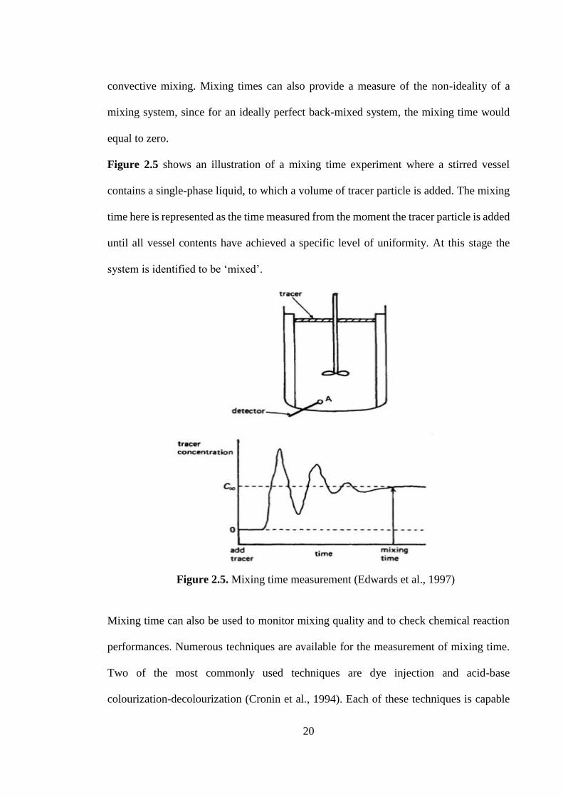
Figure 2.5 shows an illustration of a mixing time experiment where a stirred vessel
contains a single-phase liquid, to which a volume of tracer particle is added. The mixing
time here is represented as the time measured from the moment the tracer particle is added
until all vessel contents have achieved a specific level of uniformity. At this stage the
system is identified to be ‘mixed’.
Figure 2.5. Mixing time measurement (Edwards et al., 1997)
Mixing time can also be used to monitor mixing quality and to check chemical reaction
performances. Numerous techniques are available for the measurement of mixing time.
Two of the most commonly used techniques are dye injection and acid-base
colourization-decolourization (Cronin et al., 1994). Each of these techniques is capable
21
of providing accurate results for mixing time. They also allow for visual observation of
the mixing flow patterns and indicate the position of any dead zones in the vessel.
However, they cannot be used for industrial purposes as they are restricted to use in clear
vessels. This can be overcome by using an image processing technique such as Planar
Laser Induced Fluorescence (PLIF) (Chung et al., 2007; 2009) or by using the
colorimetric method (Cabaret et al., 2007).
2.2 Fluid Rheology
Fluid rheology governs several factors in mixing within a stirred vessel, such as local
hydrodynamics and phase distribution. Fluids can be described with a rheological model
that would explain fluid deformation under applied forces. Rheology refers to the study
of deformation and flow of matter at specified conditions.
This chapter aims to focus on fluid rheology of various fluids with different flow
behaviour relevant to mixing processes and intends to briefly introduce the experimental
aspects of the work of this thesis.
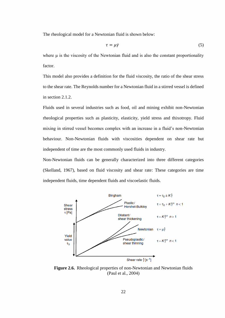
2.1.1 Newtonian and non-Newtonian Fluids
Fluids can be described as Newtonian or non-Newtonian. A fluid that has a constant
viscosity at all shear rates under constant temperature and pressures, and can be described
by a one-parameter rheological model is known as Newtonian fluid. As shown in Figure
2.6, a Newtonian material is characterised by a straight line through the origin of a shear
stress against shear rate plot.
22
The rheological model for a Newtonian fluid is shown below:
𝜏 = 𝜇�� (5)
where μ is the viscosity of the Newtonian fluid and is also the constant proportionality
factor.
This model also provides a definition for the fluid viscosity, the ratio of the shear stress
to the shear rate. The Reynolds number for a Newtonian fluid in a stirred vessel is defined
in section 2.1.2.
Fluids used in several industries such as food, oil and mining exhibit non-Newtonian
rheological properties such as plasticity, elasticity, yield stress and thixotropy. Fluid
mixing in stirred vessel becomes complex with an increase in a fluid’s non-Newtonian
behaviour. Non-Newtonian fluids with viscosities dependent on shear rate but
independent of time are the most commonly used fluids in industry.
Non-Newtonian fluids can be generally characterized into three different categories
(Skelland, 1967), based on fluid viscosity and shear rate: These categories are time
independent fluids, time dependent fluids and viscoelastic fluids.
Figure 2.6. Rheological properties of non-Newtonian and Newtonian fluids
(Paul et al., 2004)
23
Thixotropic, shear-thinning and viscoelastic fluids are most relevant to this thesis,
therefore their rheological characteristics are discussed in more detail below.
2.2.1 Viscoelastic Fluid
Viscoelastic fluids are a common type of non-Newtonian fluid. They possess both, elastic
solid and viscous fluid properties. Generally, Hookean and Newtonian materials show an
immediate response upon stress or strain addition whereas viscoelastic materials do not
respond immediately upon stress input. Viscoelastic fluids show slow partial elastic
recovery upon removal of deforming shear stress. This behaviour is referred to as creep.
Creep studies can be helpful in determining yield stresses of different materials. To do
so, a series of creep and recovery tests could be carried out in incremental stress levels.
Usually, viscoelastic fluids are macromolecular in nature, comprising of materials of high
molecular weight. Common viscoelastic fluids include polymeric fluids (melts and
solutions) used for making plastic articles, food systems such as dough making for bread,
and biological fluids such as synovial fluids found in joints (Baird, 2001).
Dynamic testing is generally feasible for measuring viscoelastic changes in fluids. Such
tests are useful in providing an assessment of product applicability along with establishing
causal relationships in problem solving efforts. Although the behaviour of viscoelastic
fluids is rheologically complex, modern rheometers are capable of easily measuring
viscoelastic responses.
24
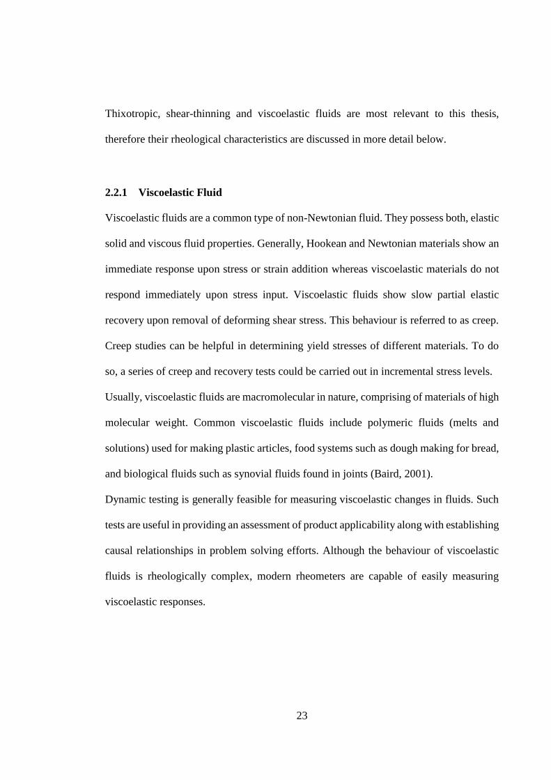
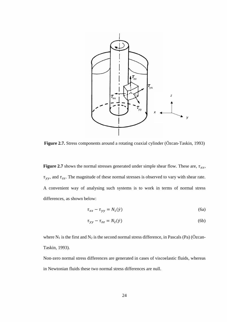
Figure 2.7. Stress components around a rotating coaxial cylinder (Özcan-Taskin, 1993)
Figure 2.7 shows the normal stresses generated under simple shear flow. These are, 𝜏𝑥𝑥,
𝜏𝑦𝑦, and 𝜏𝑧𝑧. The magnitude of these normal stresses is observed to vary with shear rate.
A convenient way of analysing such systems is to work in terms of normal stress
differences, as shown below:
𝜏𝑥𝑥 − 𝜏𝑦𝑦 = 𝑁1(��) (6a)
𝜏𝑦𝑦 − 𝜏𝑧𝑧 = 𝑁2(��) (6b)
where N1 is the first and N2 is the second normal stress difference, in Pascals (Pa) (Özcan-
Taskin, 1993).
Non-zero normal stress differences are generated in cases of viscoelastic fluids, whereas
in Newtonian fluids these two normal stress differences are null.
25
The first and second normal stress difference coefficients ѱ1 and ѱ2 (Pa.s2) respectively
are described as:
𝜓1 =𝑁1
𝛾2 (7a)
and
𝜓2 =𝑁2
𝛾2 (7b)
Similar to the shear stress and shear rate relationship, the first normal stress difference
can also be easily related to the shear rate with a power law:
𝑁1 = 𝐴𝛾 �� (8)
where the typical range of b is 1<b ≤ 2 (Özcan-Taskin, 1993).
Furthermore the Weissenberg number, (Wi), is a dimensionless number that can be used
to compare the magnitude of elastic stresses to shear stresses, shown below:
𝑊𝑖 =𝑁1
𝜏 (9)
Since the viscosity of a non-Newtonian fluid is a function of shear rate, it is referred to as
apparent viscosity and is denoted as:
𝜇𝑎 =𝜏
�� (10)
Rearranging Equation 7a gives:
𝑁1 = 𝜓1 𝛾 2 (11)
Therefore substituting for both parameters, N1 and 𝜏 gives:
𝑊𝑖 =𝑁1
𝜏=
𝜓1 𝛾2
𝜇𝑎�� (12)
26
Barnes et al (1988) proved that second normal stress differences are considered much
smaller than N1 and are negative in value. According to Weissenberg’s (1948) hypothesis,
N2 was presumed to be zero however lately it has been made possible with the use of
modern rheometers to measure non-zero N2 values with a good degree of accuracy. Even
though in some cases N2 has proven to be very crucial, for several other applications, such
as mixing, it has little practical significance and therefore is considered negligible
(Ulbrecht and Carreau, 1985).
The generation of non-zero normal stress differences is extraordinarily significant in
analysing the role of viscoelasticity in stirred vessels. Normal stress differences are
usually linked with non-linear viscoelastic effects and can be quantified as the viscoelastic
fluid property (Özcan-Taskin, 1993). Another expression of viscoelasticity is defined by
elongational viscosity, which usually shows a different behaviour as compared to shear
viscosity. This is seen in polymer solutions, which show a decrease in viscosity as shear
rate increases (shear-thinning behaviour), and show an increase in elongational viscosity
with an increase in elongational rate (Barnes et al., 1988).
2.2.2 Viscoplastic Fluid
Viscoplastic materials are another common type of non-Newtonian fluids. Apparent yield
stress is a useful parameter to describe such viscoplastic fluids. For a viscoplastic fluid to
flow, the shear stress of the material must be higher than the apparent yield stress. The
material behaves like a solid if the shear stress is below the apparent yield stress. The
Bingham plastic model shown below is a simple rheological model used for describing
viscoplastic fluids.
27
𝜏 = 𝜏𝑦 + 𝜂𝐵�� 𝑓𝑜𝑟 𝜏 > 𝜏𝑦�� = 0 𝑓𝑜𝑟 < 𝜏𝑦
(13)
The apparent viscosity of Bingham plastic materials is found to decrease as shear rate
increases, behaviour that is similar to shear-thinning fluids. Seeing as it is difficult to
measure shear stresses at very small shear rates, the yield stress is usually calculated by
extrapolating the shear stress vs shear rate plot back to zero. In this case the yield stress
is known as the apparent yield stress.
Another common type of viscoplastic model is a combination of the power law and
Bingham plastic model, known as the Herschel-Bulkley model:
𝜏 = 𝜏𝑦 + 𝑘��𝑛 𝑓𝑜𝑟 𝜏 > 𝜏𝑦�� = 0 𝑓𝑜𝑟 𝜏 < 𝜏𝑦
(14)
The Herschel-Bulkey model shown above includes the flow behaviour index (n) as
compared to the Bingham model. The fluid is represented as Bingham if n is 1, and is
referred to as Herschel-Bulkley if n is less than 1.
Adams (2009) states that viscoplastic fluids show mixing properties alike to shear-
thinning fluids, when fluid mixing is restricted near to vicinity of the impeller. However,
due to apparent yield stress, there is a fixed boundary for viscoplastic fluids whereby no
fluid motion beyond the cavern boundary is observed (Galindo and Nienow, 1992; Adams
and Barigou, 2007, Adams, 2009).
As mentioned above, the standard Reynolds number is not applicable to the power law
model, and as such the Metzner and Otto correlation needs to be used to describe the
Reynolds number for a Bingham fluid:
𝑅𝑒𝐻𝐵 =𝜌𝑘𝑠𝑁
2𝐷2
𝜏𝑦+𝜂𝐵𝑘𝑠𝑁 (15)
28
2.1.2 Thixotropic Fluid
Time-dependent fluids have a memory, or a relaxation time, which is quite long compared
to the experimental time. As shear stress is applied on such materials, they experience
changes in their physical structures. This results in the effective viscosity of the material
to change with time (Barnes, 1997).
Thixotropic fluids are one of the types of time-dependent fluids that exhibit shear-
thinning behaviour over large timescales. Upon shear stress input, the viscosity of a
thixotropic fluid decreases gradually until stress removal, after which a gradual recovery
is expected. Examples include block co-polymers and self-assembling, surfactant-based
systems (Barnes, 1997).
Another type of time dependent fluid are Rheopectic materials, which display opposite
behaviour to thixotropic materials. They exhibit shear-thickening behaviour over large
timescales and show a gradual increase in viscosity upon shear stress input, followed by
recovery upon stress removal. Examples include wood pulp and high fibre systems. The
analysis of such materials is extremely complex. Nonetheless, thixotropy fluids will be
discussed briefly in this section.
In general addition of mechanical response to stress or strain on a structured fluid causes
a varying level of viscoelasticity in the system. The microstructure may either react in a
linear way, where it does not change itself, or in a nonlinear way, where the
microstructure does change but reversibly. Complications arise in thixotropic studies
because this reversible microstructural change takes a very long time to recover, due to
the local spatial rearrangement of components. Such a long time-response makes
thixotropic studies one of the main challenges facing rheologists today, as determining
29
accurate experimental characterisation and adequate theoretical description becomes
extremely difficult and complex (Barnes, 1997).
Thixotropic materials gradually collapse upon shearing and slowly recover and rebuild at
rest. This causes difficulties in mixing and handling of such structures. In addition, the
time required to break the microstructure may take minutes but the rebuilding recovery
stage may take up to several hours. The thixotropy phenomena still needs to be
understood, and thus the need for an up-to-date review.
Early within the research on thixotropy, Scott-Blair (1943) gave a few examples of
thixotropic materials. These included clays, soil suspensions, creams, flour doughs and
suspensions, paints, and starch pastes. He was also able to define the preliminary
instruments, known as thixotrometers, specifically used to characterise thixotropy
phenomena. Another point of interest which arose was whether thixotropy should be
studied at constant shear rate or constant stress input. Furthermore, Scott-Blair showed
an easier flow in small tubes was due to thixotropy, whereas Pryce-Jones (1934, 1936,
and 1943) stated that thixotropy was more pronounced in systems containing non-
spherical particles.
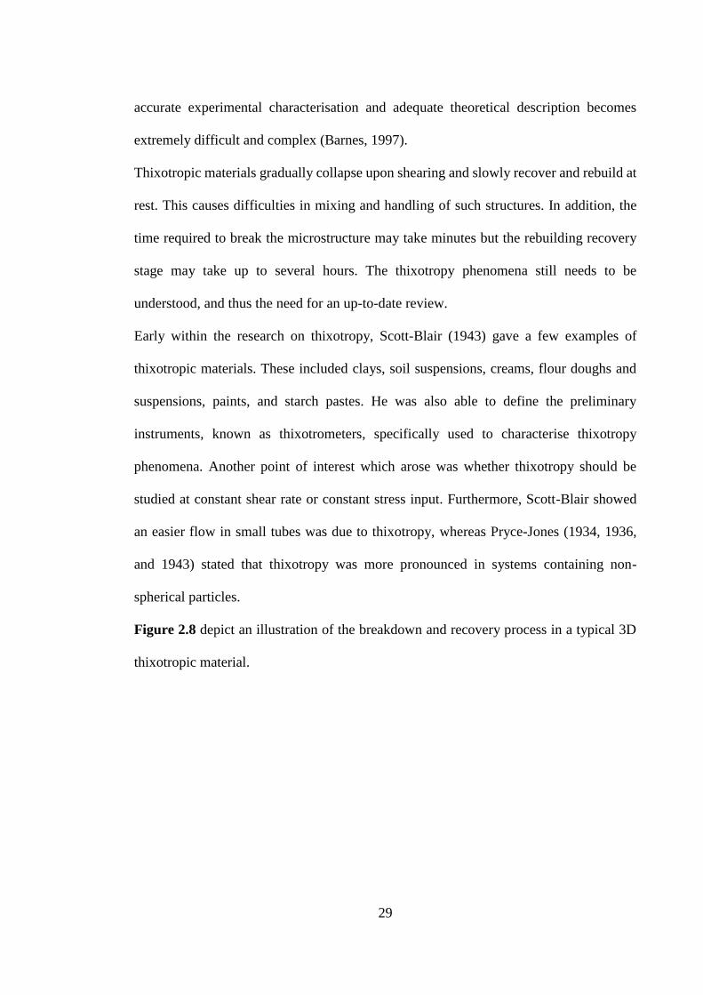
Figure 2.8 depict an illustration of the breakdown and recovery process in a typical 3D
thixotropic material.
30
Figure 2.8. Breakdown of a 3D thixotropic structure (Barnes, 1997)
There are numerous definitions of thixotropy provided in literature. These several
definitions attempt to provide a reflection on whether thixotropy is desirable or not
(Barnes, 1997). Amongst the several definitions, this thesis accepts the definition
mentioned in Polymer Technology Dictionary, "Thixotropy: A term used in rheology
which means that the viscosity of a material decreases significantly with the time of
shearing and then, increases significantly when the force inducing the flow is removed"
(Whelan, 1994)
2.3 Visualization Techniques
A large number of experimental measurement techniques have been used to quantify
mixing processes. In this section, the experimental techniques most relevant to work in
this thesis are briefly introduced. This section describes the optical techniques of Laser
Doppler Velocimetry (LDV) and Particle Image Velocimetry (PIV) for single and planar
31
flow fields. The section concisely defines the invasive technique Hot Wire Anemometry
(HWA), which can be applied to opaque fluids. It also provides a description of Planar
Laser Induced Fluorescence (PLIF) and Positron Emission Particle Tracking (PEPT)
techniques, for quantifying and tracking tracer local concentration.
2.3.1 Hot Wire Anemometry (HWA)
Hot Wire Anemometry (HWA) is an intrusive probe technique that makes use of one to
three separate wires. When the flow passes through the probe wires, a voltage pulse is
recorded which is then further translated into velocity. This technique provides a
measurement of instantaneous velocities and temperature at any instantaneous point in a
flow.
Hot wire anemometry is an ideal tool for measuring velocity fluctuations in a time domain
for turbulent flows. Gunkel and Weber (1975) made use of the HWA technique to
measure the flow of air in a baffled vessel. The technique also enabled them to measure
the pumping capacity of a six-bladed disc turbine. The technique is also capable of
providing measurements in two phase flows containing a continuous turbulent phase and
distributed bubbles.
However, since the technique is intrusive there is a risk of modification of local flow field.
As a result, the readings cannot be trusted to be entirely accurate. Moreover, the technique
is insensitive to reversal of flow direction, causing rectification error. Furthermore,
contamination is caused due to deposition of impurities on the sensor from the flow, hence
altering the calibration characteristics and reducing frequency response.
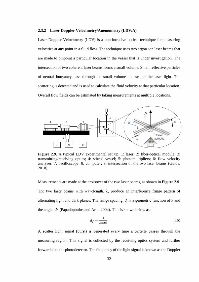
32
2.3.2 Laser Doppler Velocimetry/Anemometry (LDV/A)
Laser Doppler Velocimetry (LDV) is a non-intrusive optical technique for measuring
velocities at any point in a fluid flow. The technique uses two argon-ion laser beams that
are made to pinpoint a particular location in the vessel that is under investigation. The
intersection of two coherent laser beams forms a small volume. Small reflective particles
of neutral buoyancy pass through the small volume and scatter the laser light. The
scattering is detected and is used to calculate the fluid velocity at that particular location.
Overall flow fields can be estimated by taking measurements at multiple locations.
Figure 2.9. A typical LDV experimental set up, 1: laser; 2: fiber-optical module; 3:
transmitting/receiving optics; 4: stirred vessel; 5: photomultipliers; 6: flow velocity
analyser; 7: oscilloscope; 8: computer; 9: intersection of the two laser beams (Guida,
2010)
Measurements are made at the crossover of the two laser beams, as shown in Figure 2.9.
The two laser beams with wavelength, λ, produce an interference fringe pattern of
alternating light and dark planes. The fringe spacing, df is a geometric function of λ and
the angle, Φ, (Papadopoulos and Arik, 2004). This is shown below as:
𝑑𝑓 =𝜆
2𝑠𝑖𝑛𝜙 (16)
A scatter light signal (burst) is generated every time a particle passes through the
measuring region. This signal is collected by the receiving optics system and further
forwarded to the photodetector. The frequency of the light signal is known as the Doppler
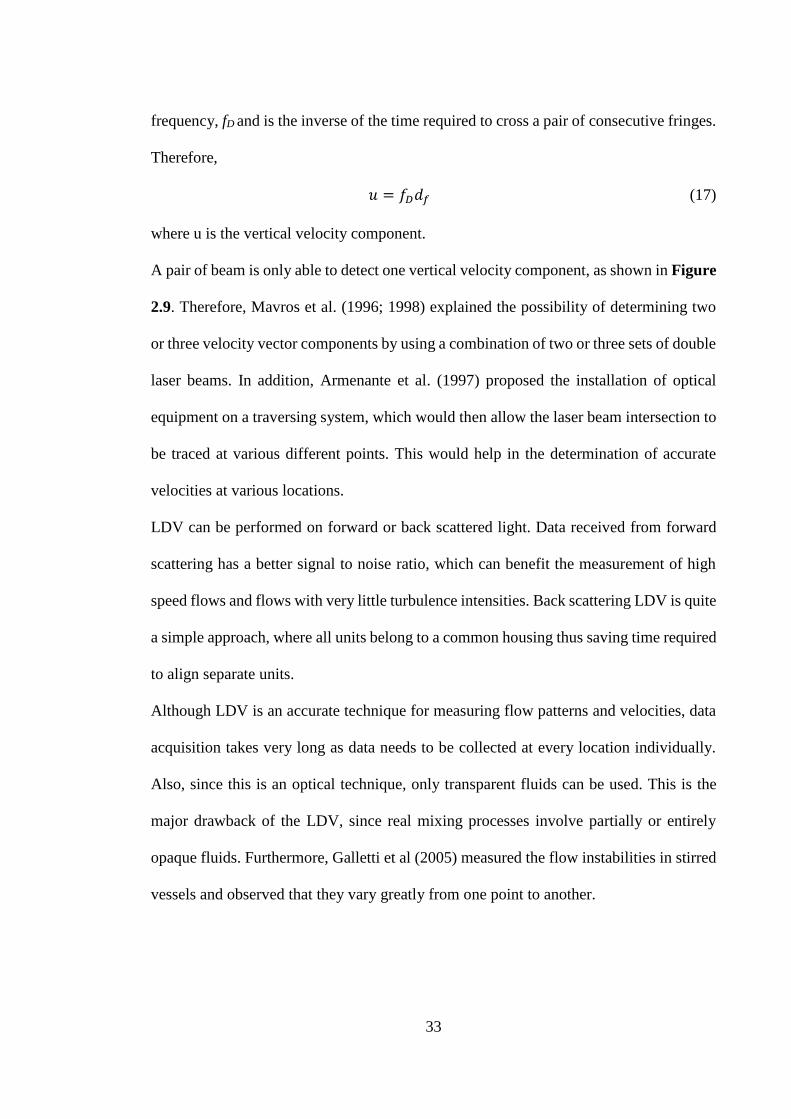
33
frequency, fD and is the inverse of the time required to cross a pair of consecutive fringes.
Therefore,
𝑢 = 𝑓𝐷𝑑𝑓 (17)
where u is the vertical velocity component.
A pair of beam is only able to detect one vertical velocity component, as shown in Figure
2.9. Therefore, Mavros et al. (1996; 1998) explained the possibility of determining two
or three velocity vector components by using a combination of two or three sets of double
laser beams. In addition, Armenante et al. (1997) proposed the installation of optical
equipment on a traversing system, which would then allow the laser beam intersection to
be traced at various different points. This would help in the determination of accurate
velocities at various locations.
LDV can be performed on forward or back scattered light. Data received from forward
scattering has a better signal to noise ratio, which can benefit the measurement of high
speed flows and flows with very little turbulence intensities. Back scattering LDV is quite
a simple approach, where all units belong to a common housing thus saving time required
to align separate units.
Although LDV is an accurate technique for measuring flow patterns and velocities, data
acquisition takes very long as data needs to be collected at every location individually.
Also, since this is an optical technique, only transparent fluids can be used. This is the
major drawback of the LDV, since real mixing processes involve partially or entirely
opaque fluids. Furthermore, Galletti et al (2005) measured the flow instabilities in stirred
vessels and observed that they vary greatly from one point to another.
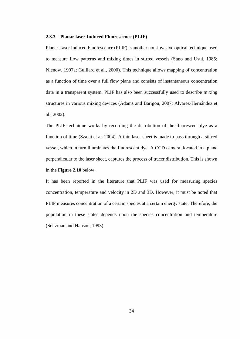
34
2.3.3 Planar laser Induced Fluorescence (PLIF)
Planar Laser Induced Fluorescence (PLIF) is another non-invasive optical technique used
to measure flow patterns and mixing times in stirred vessels (Sano and Usui, 1985;
Nienow, 1997a; Guillard et al., 2000). This technique allows mapping of concentration
as a function of time over a full flow plane and consists of instantaneous concentration
data in a transparent system. PLIF has also been successfully used to describe mixing
structures in various mixing devices (Adams and Barigou, 2007; Alvarez-Hernández et
al., 2002).
The PLIF technique works by recording the distribution of the fluorescent dye as a
function of time (Szalai et al. 2004). A thin laser sheet is made to pass through a stirred
vessel, which in turn illuminates the fluorescent dye. A CCD camera, located in a plane
perpendicular to the laser sheet, captures the process of tracer distribution. This is shown
in the Figure 2.10 below.
It has been reported in the literature that PLIF was used for measuring species
concentration, temperature and velocity in 2D and 3D. However, it must be noted that
PLIF measures concentration of a certain species at a certain energy state. Therefore, the
population in these states depends upon the species concentration and temperature
(Seitzman and Hanson, 1993).
35
Figure 2.10. Simplified PLIF experimental facility.
Bakker and Van den Akker (1996) made use of the PLIF technique to measure the yield
of a reactor system operating in a turbulent flow. Guillard et al. (2000) performed a study
on turbulent flows in a stirred vessel and showed that PLIF is capable of revealing the
presence of coherent mixing structures and detecting strong tangential flows in the
impeller stream. PLIF has also been used to measure flow structures in stirred vessels
with disc impellers (Fountain et al., 2000), to study flow patterns in the laminar regime
for a variety of impellers (Alvarez-Hernández et al., 2002, and Szalai et al., 2004) and to
investigate eccentric agitation in small, unbaffled vessels (Hall et al., 2005a).
Whereras PLIF has several benefits, it must be noted that it is unable to measure
velocities. In addition, as in the case of LDV, this technique can only be used on
transparent fluids.
2.3.4 Particle Image Velocimetry (PIV)
Particle Image Velocimetry (PIV) is a well-known, non-invasive, optical Eulerian
technique used for measuring instantaneous flow in translucent systems. It is capable of
36
providing 2D Eulerian data by measuring velocities on a laser plane. The technique has
made major contribution to the research of complex hydrodynamics in stirred vessels. A
number of researchers have listed the principles of PIV such as Lourenco et al. (1989),
Adrian (1991), and Willert and Gharib (1991).
The PIV set-up comprises of a laser emission unit and a camera for recording images, as
shown in Figure 2.11. Both of these are controlled by a synchronizer. The laser emission
unit illuminates a cross-section of the seeded flow field. The recording camera is located
in a plane perpendicular to the light sheet and a data processor is used for analysing
images. A small quantity of seeding tracer particles are suspended in a transparent fluid.
Tracer particles are illuminated by a pulsing, thin plane of laser sheet and seeding particles
are located by image recording. These images are then divided into several small
interrogation areas (IA). Fast Fourier Transform (FFT) cross correlation helps determine
the displacement of seeding tracer particles in the IA.
Figure 2.11. Simplified, typical PIV set-up, Image taken from (Guida, 2010)
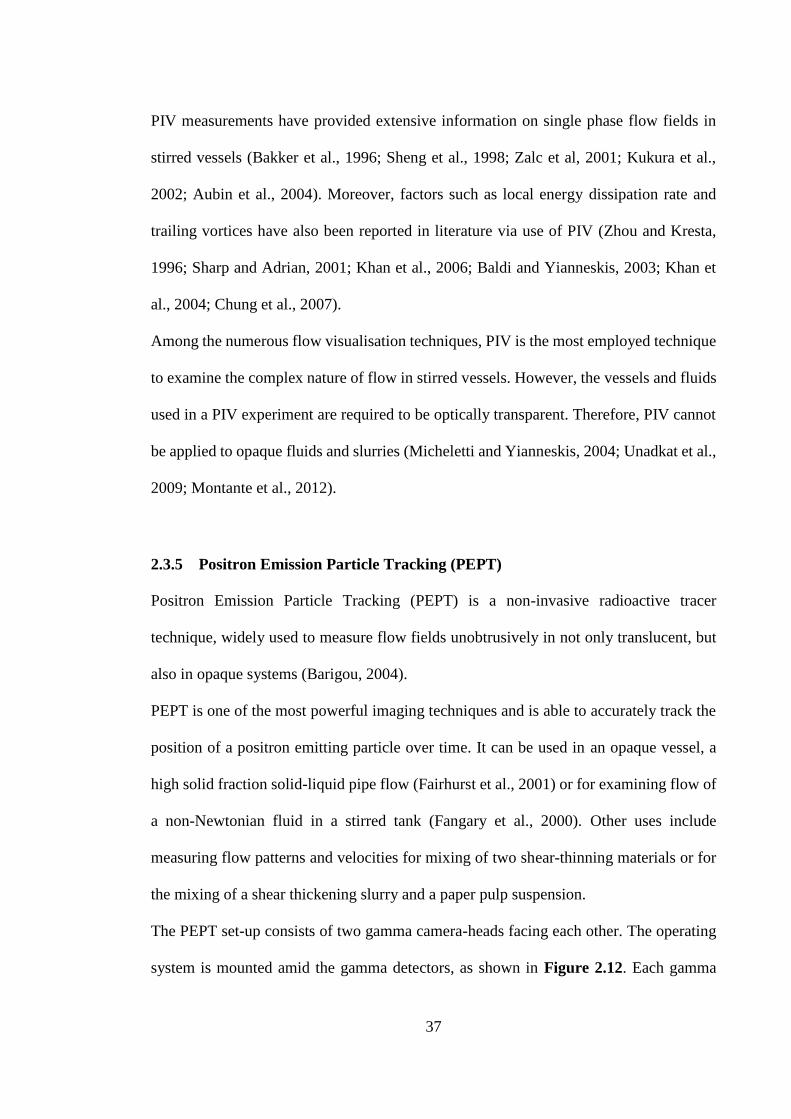
37
PIV measurements have provided extensive information on single phase flow fields in
stirred vessels (Bakker et al., 1996; Sheng et al., 1998; Zalc et al, 2001; Kukura et al.,
2002; Aubin et al., 2004). Moreover, factors such as local energy dissipation rate and
trailing vortices have also been reported in literature via use of PIV (Zhou and Kresta,
1996; Sharp and Adrian, 2001; Khan et al., 2006; Baldi and Yianneskis, 2003; Khan et
al., 2004; Chung et al., 2007).
Among the numerous flow visualisation techniques, PIV is the most employed technique
to examine the complex nature of flow in stirred vessels. However, the vessels and fluids
used in a PIV experiment are required to be optically transparent. Therefore, PIV cannot
be applied to opaque fluids and slurries (Micheletti and Yianneskis, 2004; Unadkat et al.,
2009; Montante et al., 2012).
2.3.5 Positron Emission Particle Tracking (PEPT)
Positron Emission Particle Tracking (PEPT) is a non-invasive radioactive tracer
technique, widely used to measure flow fields unobtrusively in not only translucent, but
also in opaque systems (Barigou, 2004).
PEPT is one of the most powerful imaging techniques and is able to accurately track the
position of a positron emitting particle over time. It can be used in an opaque vessel, a
high solid fraction solid-liquid pipe flow (Fairhurst et al., 2001) or for examining flow of
a non-Newtonian fluid in a stirred tank (Fangary et al., 2000). Other uses include
measuring flow patterns and velocities for mixing of two shear-thinning materials or for
the mixing of a shear thickening slurry and a paper pulp suspension.
The PEPT set-up consists of two gamma camera-heads facing each other. The operating
system is mounted amid the gamma detectors, as shown in Figure 2.12. Each gamma
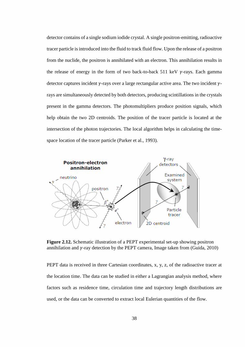
38
detector contains of a single sodium iodide crystal. A single positron-emitting, radioactive
tracer particle is introduced into the fluid to track fluid flow. Upon the release of a positron
from the nuclide, the positron is annihilated with an electron. This annihilation results in
the release of energy in the form of two back-to-back 511 keV 𝛾-rays. Each gamma
detector captures incident 𝛾-rays over a large rectangular active area. The two incident 𝛾-
rays are simultaneously detected by both detectors, producing scintillations in the crystals
present in the gamma detectors. The photomultipliers produce position signals, which
help obtain the two 2D centroids. The position of the tracer particle is located at the
intersection of the photon trajectories. The local algorithm helps in calculating the time-
space location of the tracer particle (Parker et al., 1993).
Figure 2.12. Schematic illustration of a PEPT experimental set-up showing positron
annihilation and 𝛾-ray detection by the PEPT camera, Image taken from (Guida, 2010)
PEPT data is received in three Cartesian coordinates, x, y, z, of the radioactive tracer at
the location time. The data can be studied in either a Lagrangian analysis method, where
factors such as residence time, circulation time and trajectory length distributions are
used, or the data can be converted to extract local Eulerian quantities of the flow.
39
PEPT has been employed widely to study flows in several different situations. Pianko-
Oprych et al. (2009) compared the use of PEPT with PIV for measurement of turbulent
water flow in a stirred vessel and found that the results obtained by PEPT were accurate
and reliable. Fangary et al. (1999, 2000, and 2002) used PEPT data for studying the
agitation of non-Newtonian fluids in a stirred vessel. They were able to obtain particle
trajectory-length distribution and to estimate fluid circulation time. Eulerian data for
shear-thinning and visco-plastic fluids from PEPT measurements was analysed by Adams
et al. (2008, 2009). PEPT has also been used to study solid-liquid flows in stirred vessels
(Barigou et al., 2009) and multiphase flows to map fluid flow (Parker et al., 2002;
Barigou, 2004).
40
3 Chapter 3
Experimental Techniques and Theoretical Analysis
Stirred vessels are the most common mixing equipment used in the industries, for
example they are used in the processing industry for blending miscible liquids. This
chapter presents a description of the equipment used, followed by a description of the
experimental techniques. Particle Image Velocimetry (PIV) is a non-intrusive
visualisation technique applied for measuring instantaneous flow velocity and to thus
improve studies of fluid with complex rheology mixed in stirred vessels. 2D Eulerian data
can be obtained by PIV by measuring the flow velocities of the fluid present on a laser
plane going through the stirred tank. The Planer Laser Induced Fuorescence (PLIF)
visualisation technique was also was employed in this study to invistigate flow behaviour
of non-Newtonian fluids over mixing time. Theoretical analysis of 2D data measurements
obtained from PIV is discussed later in this chapter. The material of test fluids used in
this work and the rheology of these fluids is discussed in each results chapter separately.
3.1 Apparatus
One rig was used for both the PIV and PLIF experiments conducted in this study for all
fluids. The cylindrical glass stirred vessel used in this work contained a flat-base of
diameter T=115 mm. In order to reduce light distortion, the stirred vessel was placed
inside a water-filled square glass tank. Four wall baffles of width B = 0.1T were equally
spaced within the vessel, as shown in Figure 3.1a.
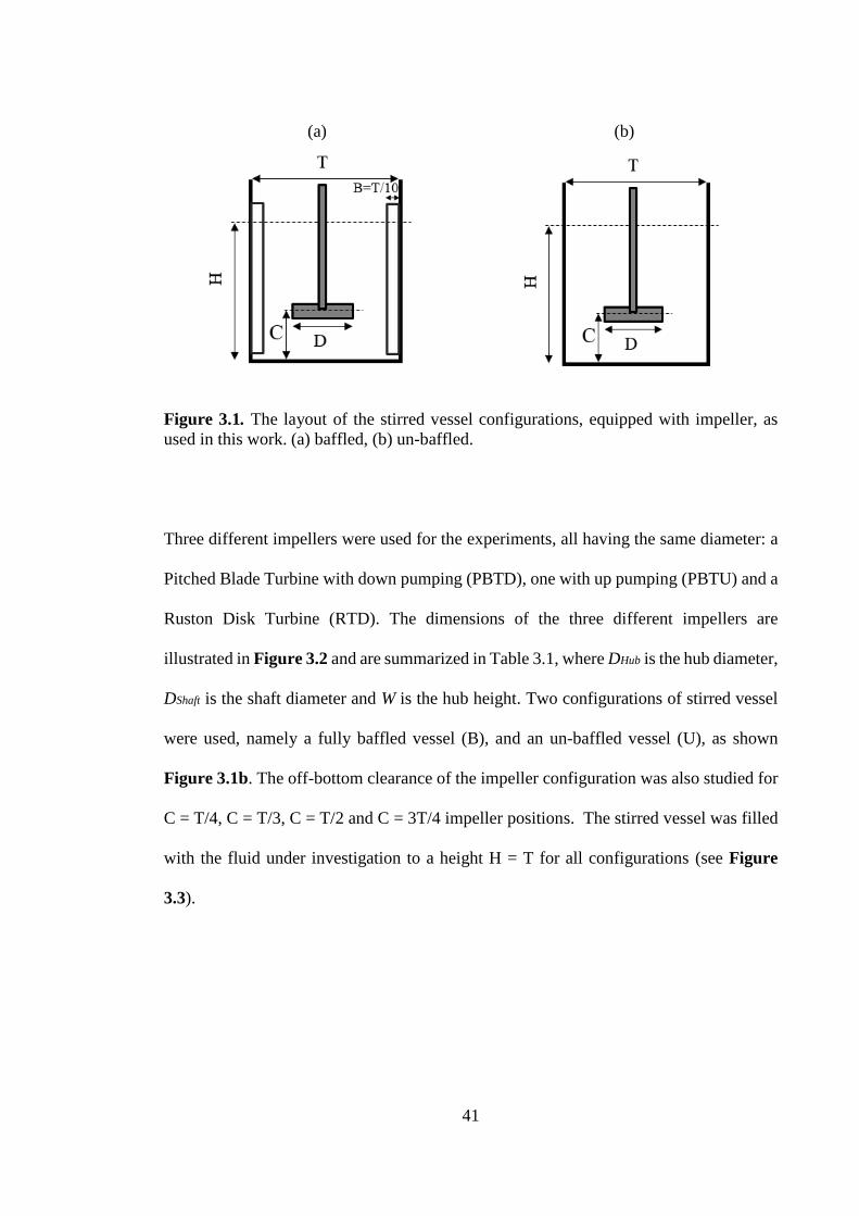
41
(a) (b)
Figure 3.1. The layout of the stirred vessel configurations, equipped with impeller, as
used in this work. (a) baffled, (b) un-baffled.
Three different impellers were used for the experiments, all having the same diameter: a
Pitched Blade Turbine with down pumping (PBTD), one with up pumping (PBTU) and a
Ruston Disk Turbine (RTD). The dimensions of the three different impellers are
illustrated in Figure 3.2 and are summarized in Table 3.1, where DHub is the hub diameter,
DShaft is the shaft diameter and W is the hub height. Two configurations of stirred vessel
were used, namely a fully baffled vessel (B), and an un-baffled vessel (U), as shown
Figure 3.1b. The off-bottom clearance of the impeller configuration was also studied for
C = T/4, C = T/3, C = T/2 and C = 3T/4 impeller positions. The stirred vessel was filled
with the fluid under investigation to a height H = T for all configurations (see Figure
3.3).
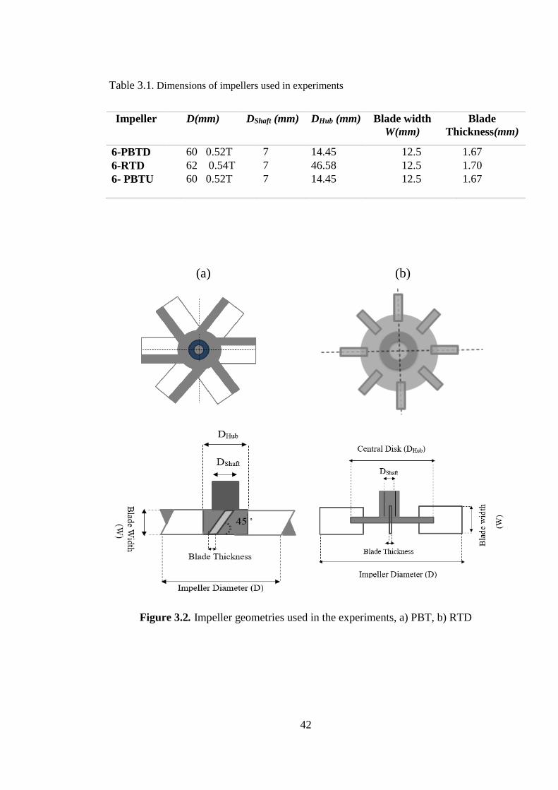
42
Table 3.1. Dimensions of impellers used in experiments
Figure 3.2. Impeller geometries used in the experiments, a) PBT, b) RTD
Impeller D(mm) DShaft (mm) DHub (mm) Blade width
W(mm)
Blade
Thickness(mm)
6-PBTD 60 0.52T 7 14.45 12.5 1.67
6-RTD 62 0.54T 7 46.58 12.5 1.70
6- PBTU 60 0.52T 7 14.45 12.5 1.67
(a)
(b)
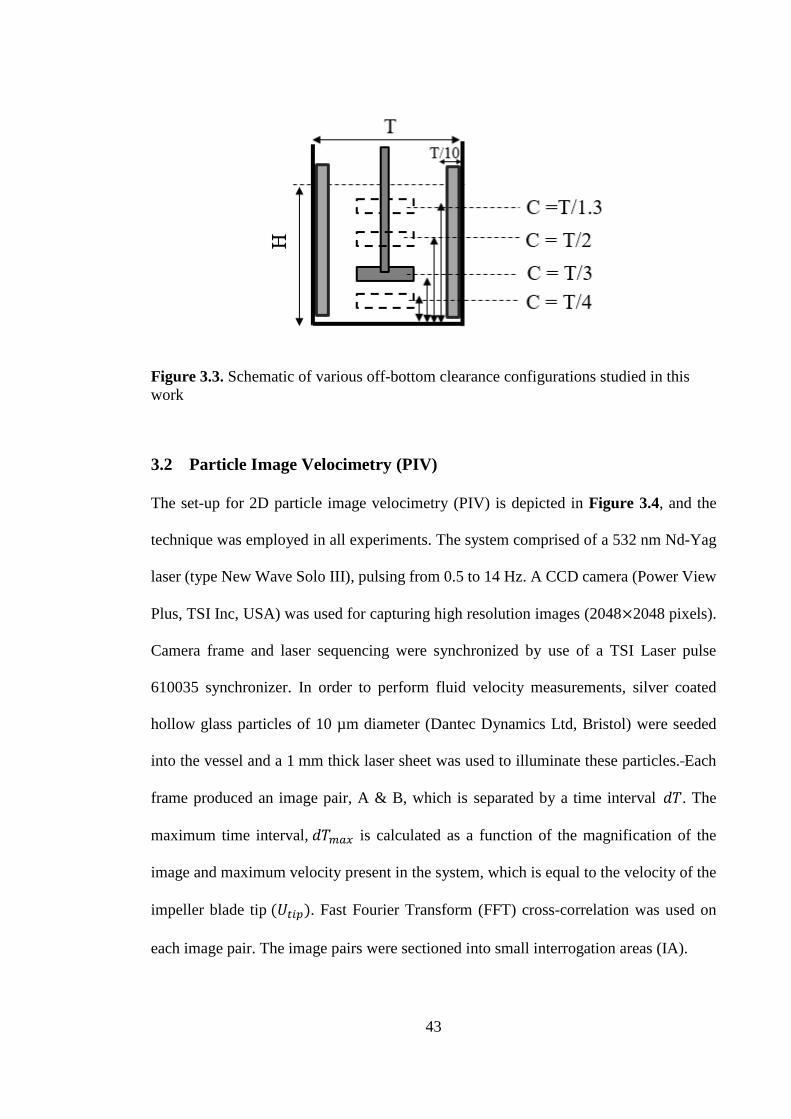
43
Figure 3.3. Schematic of various off-bottom clearance configurations studied in this
work
3.2 Particle Image Velocimetry (PIV)
The set-up for 2D particle image velocimetry (PIV) is depicted in Figure 3.4, and the
technique was employed in all experiments. The system comprised of a 532 nm Nd-Yag
laser (type New Wave Solo III), pulsing from 0.5 to 14 Hz. A CCD camera (Power View
Plus, TSI Inc, USA) was used for capturing high resolution images (2048×2048 pixels).
Camera frame and laser sequencing were synchronized by use of a TSI Laser pulse
610035 synchronizer. In order to perform fluid velocity measurements, silver coated
hollow glass particles of 10 µm diameter (Dantec Dynamics Ltd, Bristol) were seeded
into the vessel and a 1 mm thick laser sheet was used to illuminate these particles. Each
frame produced an image pair, A & B, which is separated by a time interval 𝑑𝑇. The
maximum time interval, 𝑑𝑇𝑚𝑎𝑥 is calculated as a function of the magnification of the
image and maximum velocity present in the system, which is equal to the velocity of the
impeller blade tip (𝑈𝑡𝑖𝑝). Fast Fourier Transform (FFT) cross-correlation was used on
each image pair. The image pairs were sectioned into small interrogation areas (IA).
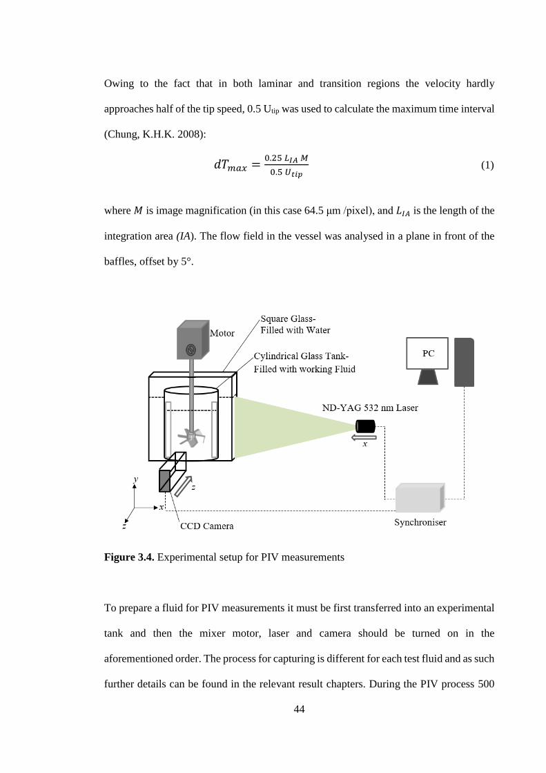
44
Owing to the fact that in both laminar and transition regions the velocity hardly
approaches half of the tip speed, 0.5 Utip was used to calculate the maximum time interval
(Chung, K.H.K. 2008):
𝑑𝑇𝑚𝑎𝑥 =0.25 𝐿𝐼𝐴 𝑀
0.5 𝑈𝑡𝑖𝑝 (1)
where 𝑀 is image magnification (in this case 64.5 μm /pixel), and 𝐿𝐼𝐴 is the length of the
integration area (IA). The flow field in the vessel was analysed in a plane in front of the
baffles, offset by 5°.
Figure 3.4. Experimental setup for PIV measurements
To prepare a fluid for PIV measurements it must be first transferred into an experimental
tank and then the mixer motor, laser and camera should be turned on in the
aforementioned order. The process for capturing is different for each test fluid and as such
further details can be found in the relevant result chapters. During the PIV process 500
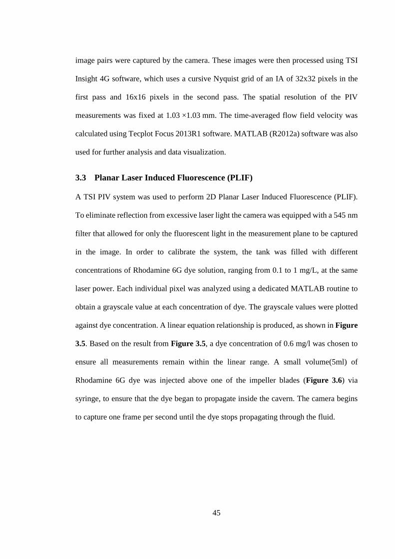
45
image pairs were captured by the camera. These images were then processed using TSI
Insight 4G software, which uses a cursive Nyquist grid of an IA of 32x32 pixels in the
first pass and 16x16 pixels in the second pass. The spatial resolution of the PIV
measurements was fixed at 1.03 ×1.03 mm. The time-averaged flow field velocity was
calculated using Tecplot Focus 2013R1 software. MATLAB (R2012a) software was also
used for further analysis and data visualization.
3.3 Planar Laser Induced Fluorescence (PLIF)
A TSI PIV system was used to perform 2D Planar Laser Induced Fluorescence (PLIF).
To eliminate reflection from excessive laser light the camera was equipped with a 545 nm
filter that allowed for only the fluorescent light in the measurement plane to be captured
in the image. In order to calibrate the system, the tank was filled with different
concentrations of Rhodamine 6G dye solution, ranging from 0.1 to 1 mg/L, at the same
laser power. Each individual pixel was analyzed using a dedicated MATLAB routine to
obtain a grayscale value at each concentration of dye. The grayscale values were plotted
against dye concentration. A linear equation relationship is produced, as shown in Figure
3.5. Based on the result from Figure 3.5, a dye concentration of 0.6 mg/l was chosen to
ensure all measurements remain within the linear range. A small volume(5ml) of
Rhodamine 6G dye was injected above one of the impeller blades (Figure 3.6) via
syringe, to ensure that the dye began to propagate inside the cavern. The camera begins
to capture one frame per second until the dye stops propagating through the fluid.
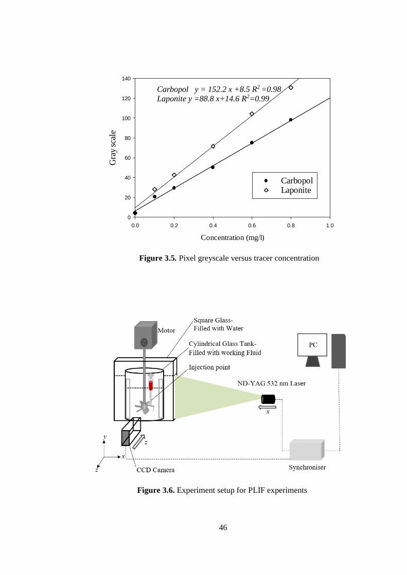
46
Figure 3.5. Pixel greyscale versus tracer concentration
Figure 3.6. Experiment setup for PLIF experiments
Concentration (mg/l)
0.0 0.2 0.4 0.6 0.8 1.0
Gra
y sc
ale
0
20
40
60
80
100
120
140
CarbopolLaponite
Carbopol y = 152.2 x +8.5 R2 =0.98
Laponite y =88.8 x+14.6 R2=0.99
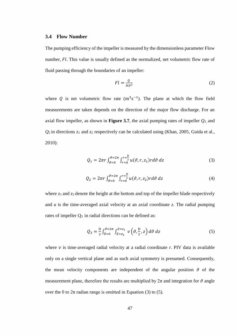
47
3.4 Flow Number
The pumping efficiency of the impeller is measured by the dimensionless parameter Flow
number, 𝐹𝑙. This value is usually defined as the normalized, net volumetric flow rate of
fluid passing through the boundaries of an impeller:
𝐹𝑙 =𝑄
𝑁𝐷3 (2)
where 𝑄 is net volumetric flow rate (m3s−1). The plane at which the flow field
measurements are taken depends on the direction of the major flow discharge. For an
axial flow impeller, as shown in Figure 3.7, the axial pumping rates of impeller Q1, and
Q2 in directions z1 and z2 respectively can be calculated using (Khan, 2005, Guida et al.,
2010):
𝑄1 = 2𝜋𝑟 ∫ ∫ 𝑢(𝜗, 𝑟, 𝑧1)𝑟𝑑𝜗 𝑑𝑧𝑟=
D
2𝑟=0
𝜗=2𝜋
𝜗=0 (3)
𝑄2 = 2𝜋𝑟 ∫ ∫ 𝑢(𝜗, 𝑟, 𝑧2)𝑟𝑑𝜗 𝑑𝑧𝑟=
𝐷
2𝑟=0
𝜗=2𝜋
𝜗=0 (4)
where z1 and z2 denote the height at the bottom and top of the impeller blade respectively
and u is the time-averaged axial velocity at an axial coordinate z. The radial pumping
rates of impeller Q3 in radial directions can be defined as:
𝑄3 =D
2∫ ∫ 𝑣 (𝜗,
D
2, 𝑧) 𝑑𝜗 𝑑𝑧
𝑍=𝑧1
𝑍=𝑧2
𝜗=2𝜋
𝜗=0 (5)
where 𝑣 is time-averaged radial velocity at a radial coordinate r. PIV data is available
only on a single vertical plane and as such axial symmetry is presumed. Consequently,
the mean velocity components are independent of the angular position 𝜗 of the
measurement plane, therefore the results are multiplied by 2π and integration for 𝜗 angle
over the 0 to 2π radian range is omitted in Equation (3) to (5).
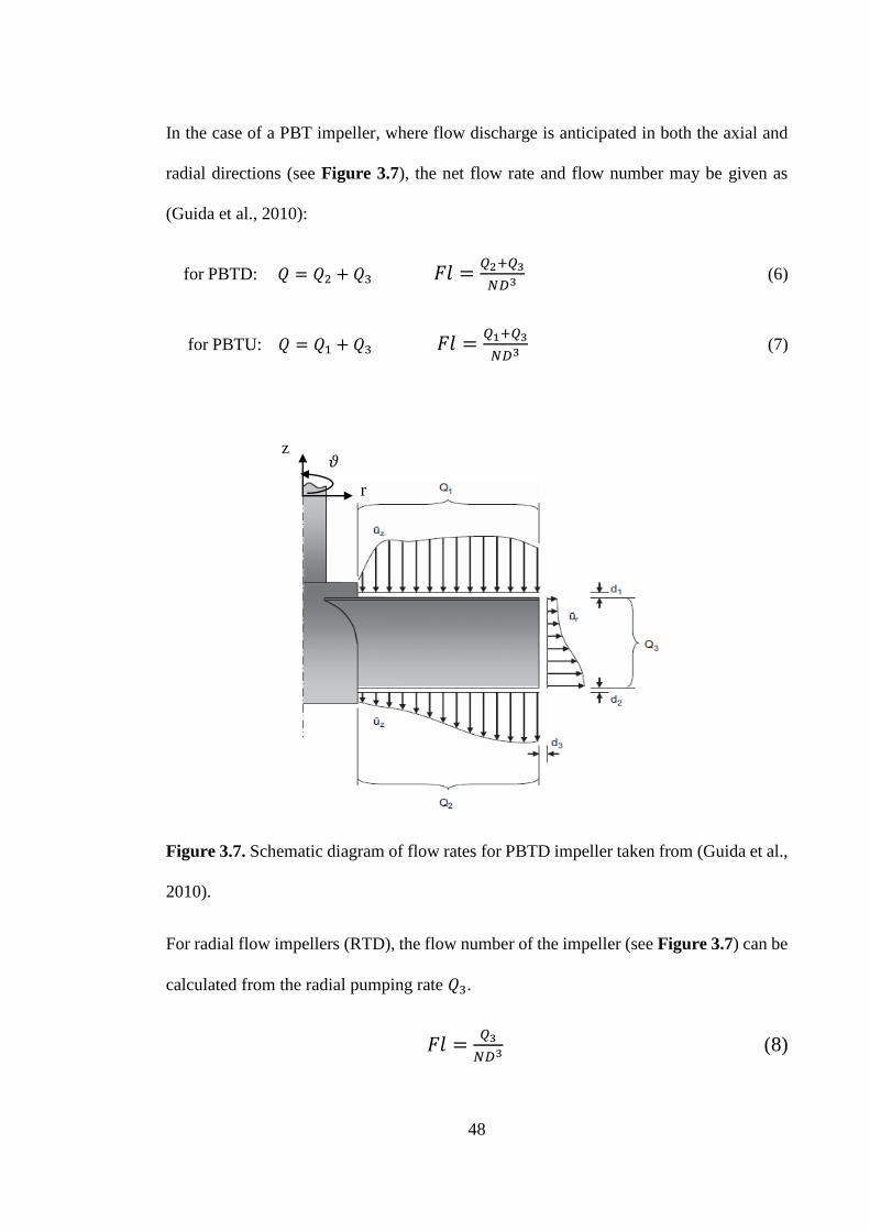
48
In the case of a PBT impeller, where flow discharge is anticipated in both the axial and
radial directions (see Figure 3.7), the net flow rate and flow number may be given as
(Guida et al., 2010):
for PBTD: 𝑄 = 𝑄2 + 𝑄3 𝐹𝑙 =𝑄2+𝑄3
𝑁𝐷3 (6)
for PBTU: 𝑄 = 𝑄1 + 𝑄3 𝐹𝑙 =𝑄1+𝑄3
𝑁𝐷3 (7)
Figure 3.7. Schematic diagram of flow rates for PBTD impeller taken from (Guida et al.,
2010).
For radial flow impellers (RTD), the flow number of the impeller (see Figure 3.7) can be
calculated from the radial pumping rate 𝑄3.
𝐹𝑙 =𝑄3
𝑁𝐷3 (8)
r
z 𝜗
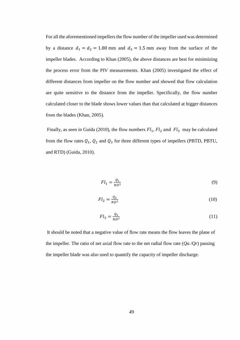
49
For all the aforementioned impellers the flow number of the impeller used was determined
by a distance 𝑑1 = 𝑑2 = 1.80 mm and 𝑑3 = 1.5 mm away from the surface of the
impeller blades. According to Khan (2005), the above distances are best for minimizing
the process error from the PIV measurements. Khan (2005) investigated the effect of
different distances from impeller on the flow number and showed that flow calculation
are quite sensitive to the distance from the impeller. Specifically, the flow number
calculated closer to the blade shows lower values than that calculated at bigger distances
from the blades (Khan, 2005).
Finally, as seen in Guida (2010), the flow numbers 𝐹𝑙1, 𝐹𝑙2 and 𝐹𝑙3 may be calculated
from the flow rates 𝑄1, 𝑄2 and 𝑄3 for three different types of impellers (PBTD, PBTU,
and RTD) (Guida, 2010).
𝐹𝑙1 =𝑄1
𝑁𝐷3 (9)
𝐹𝑙2 =𝑄2
𝑁𝐷3 (10)
𝐹𝑙3 =𝑄3
𝑁𝐷3 (11)
It should be noted that a negative value of flow rate means the flow leaves the plane of
the impeller. The ratio of net axial flow rate to the net radial flow rate (Qa /Qr) passing
the impeller blade was also used to quantify the capacity of impeller discharge.
50
4 Chapter 4
EFFECT OF THIXOROPY ON FLUID MIXING IN A
STIRRED TANK
The aim of this work is to investigate the effects of time dependency on fluid mixing in a
stirred vessel. To achieve this various rheological variable were fixed by choosing a time
independent reference fluid that exhibited the similar rheological properties as the main
fluid of this study.
The PIV technique is employed to characterize the flow fields of a transparent, colloidal
dispersion of 2.2 w% Laponite thixotropic fluid in a stirred tank for three mixing regimes:
ReHB = 7, ReHB = 61 and ReHB =158. A time independent transparent, aqueous 1w%
Carbopol fluid that exhibited similar rheological properties behaviour is used as reference
fluid to help to distinguish time effect from other rheological properties of the time-
dependent 2.2w% Laponite fluid. The PLIF visualization technique is applied to further
investigate the evolution of the cavern volume with time. The mixing efficiency of the
impellers is analysed in terms of size and growth of a cavern over time and impeller
pumping efficiency. Furthermore, the effect of impeller bottom clearance with three
impellers (PBTU, PBTD, and RTD) in the mixing of a thixotropic fluid was investigated.
Finally, an un-baffled stirred tank configuration was investigated to understand mixing
performance in terms of cavern size and growth and flow fields.
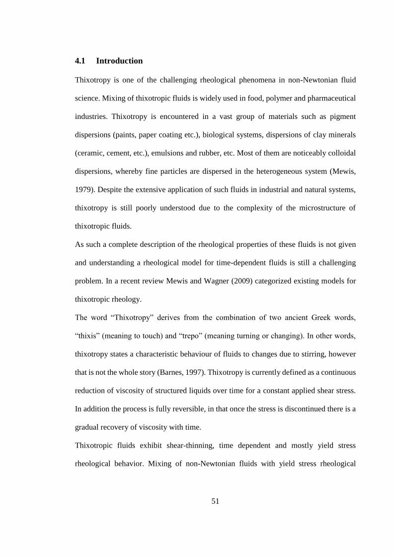
51
4.1 Introduction
Thixotropy is one of the challenging rheological phenomena in non-Newtonian fluid
science. Mixing of thixotropic fluids is widely used in food, polymer and pharmaceutical
industries. Thixotropy is encountered in a vast group of materials such as pigment
dispersions (paints, paper coating etc.), biological systems, dispersions of clay minerals
(ceramic, cement, etc.), emulsions and rubber, etc. Most of them are noticeably colloidal
dispersions, whereby fine particles are dispersed in the heterogeneous system (Mewis,
1979). Despite the extensive application of such fluids in industrial and natural systems,
thixotropy is still poorly understood due to the complexity of the microstructure of
thixotropic fluids.
As such a complete description of the rheological properties of these fluids is not given
and understanding a rheological model for time-dependent fluids is still a challenging
problem. In a recent review Mewis and Wagner (2009) categorized existing models for
thixotropic rheology.
The word “Thixotropy” derives from the combination of two ancient Greek words,
“thixis” (meaning to touch) and “trepo” (meaning turning or changing). In other words,
thixotropy states a characteristic behaviour of fluids to changes due to stirring, however
that is not the whole story (Barnes, 1997). Thixotropy is currently defined as a continuous
reduction of viscosity of structured liquids over time for a constant applied shear stress.
In addition the process is fully reversible, in that once the stress is discontinued there is a
gradual recovery of viscosity with time.
Thixotropic fluids exhibit shear-thinning, time dependent and mostly yield stress
rheological behavior. Mixing of non-Newtonian fluids with yield stress rheological
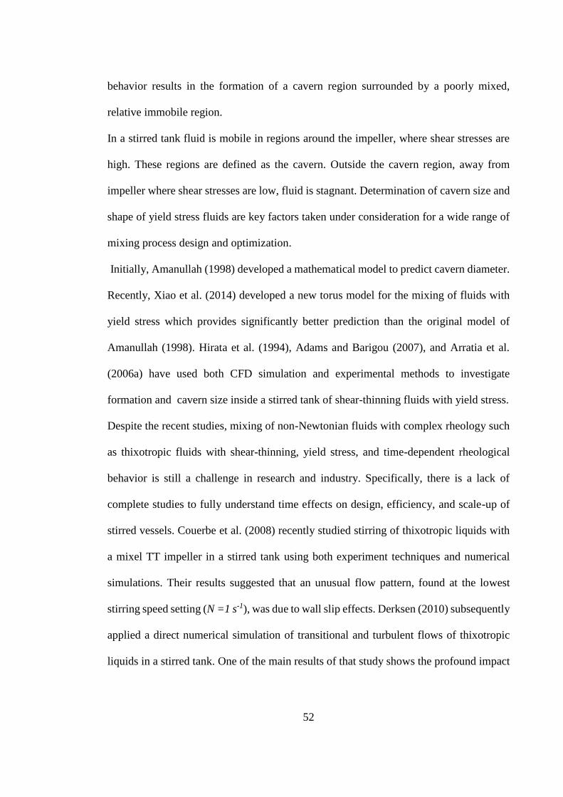
52
behavior results in the formation of a cavern region surrounded by a poorly mixed,
relative immobile region.
In a stirred tank fluid is mobile in regions around the impeller, where shear stresses are
high. These regions are defined as the cavern. Outside the cavern region, away from
impeller where shear stresses are low, fluid is stagnant. Determination of cavern size and
shape of yield stress fluids are key factors taken under consideration for a wide range of
mixing process design and optimization.
Initially, Amanullah (1998) developed a mathematical model to predict cavern diameter.
Recently, Xiao et al. (2014) developed a new torus model for the mixing of fluids with
yield stress which provides significantly better prediction than the original model of
Amanullah (1998). Hirata et al. (1994), Adams and Barigou (2007), and Arratia et al.
(2006a) have used both CFD simulation and experimental methods to investigate
formation and cavern size inside a stirred tank of shear-thinning fluids with yield stress.
Despite the recent studies, mixing of non-Newtonian fluids with complex rheology such
as thixotropic fluids with shear-thinning, yield stress, and time-dependent rheological
behavior is still a challenge in research and industry. Specifically, there is a lack of
complete studies to fully understand time effects on design, efficiency, and scale-up of
stirred vessels. Couerbe et al. (2008) recently studied stirring of thixotropic liquids with
a mixel TT impeller in a stirred tank using both experiment techniques and numerical
simulations. Their results suggested that an unusual flow pattern, found at the lowest
stirring speed setting (N =1 s-1), was due to wall slip effects. Derksen (2010) subsequently
applied a direct numerical simulation of transitional and turbulent flows of thixotropic
liquids in a stirred tank. One of the main results of that study shows the profound impact
53
of the liquids’ relaxation time - characterized by the dimensionless Deborah number on
the flow patterns in the mixing tanks.
4.2 Material and Experimental Design
4.2.1 Rheology of Test Fluids
4.2.1.1 Time Dependent Fluids (Thixotropy)
The non-Newtonian fluid chosen for investigation was a 2.2w% Laponite (Laponite RD,
conservation resources UK Ltd) dispersion in distilled water. Laponite, a synthetic
layered silicate, is an additive which improves performance and properties of an extensive
range of industrial and consumer products such as surface coatings, household cleaners
and personal care products. This component allows a controlled rate of restructuring after
applied shear and improves the stability of a product. Laponite is also used as a film
former agent to produce electrically conductive, antistatic and barrier coatings.
Laponite fluids exhibit thixotropic, shear-thinning and yield stress properties. The
detailed properties of this fluid are discussed in detail in the work of Coussot et al. (2002),
Coussot et al. (1993) and Bonn et al. (2002).
The fluid is prepared according to the preparation method described in Couerbe et al.
(2008). Laponite powder was added gradually in agitated distilled water and left to fully
mix for one hour at N = 7 s-1. 6 ppm of NaCl was then added to the stirring liquid so as
to increase the pH of the fluid to approximately pH = 10. When the process was completed
a clear, colorless colloidal dispersion was produced. The prepared fluid was then left at
rest for a few days to complete absorption of water molecules into the powder (solid
matrix), a process needed in order to prevent irreversible aging during the experiments
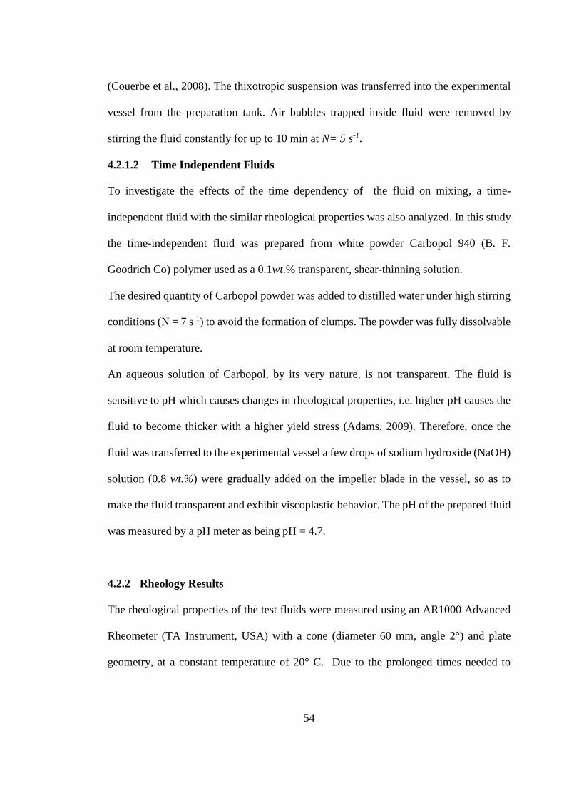
54
(Couerbe et al., 2008). The thixotropic suspension was transferred into the experimental
vessel from the preparation tank. Air bubbles trapped inside fluid were removed by
stirring the fluid constantly for up to 10 min at N= 5 s-1.
4.2.1.2 Time Independent Fluids
To investigate the effects of the time dependency of the fluid on mixing, a time-
independent fluid with the similar rheological properties was also analyzed. In this study
the time-independent fluid was prepared from white powder Carbopol 940 (B. F.
Goodrich Co) polymer used as a 0.1wt.% transparent, shear-thinning solution.
The desired quantity of Carbopol powder was added to distilled water under high stirring
conditions (N = 7 s-1) to avoid the formation of clumps. The powder was fully dissolvable
at room temperature.
An aqueous solution of Carbopol, by its very nature, is not transparent. The fluid is
sensitive to pH which causes changes in rheological properties, i.e. higher pH causes the
fluid to become thicker with a higher yield stress (Adams, 2009). Therefore, once the
fluid was transferred to the experimental vessel a few drops of sodium hydroxide (NaOH)
solution (0.8 wt.%) were gradually added on the impeller blade in the vessel, so as to
make the fluid transparent and exhibit viscoplastic behavior. The pH of the prepared fluid
was measured by a pH meter as being pH = 4.7.
4.2.2 Rheology Results
The rheological properties of the test fluids were measured using an AR1000 Advanced
Rheometer (TA Instrument, USA) with a cone (diameter 60 mm, angle 2°) and plate
geometry, at a constant temperature of 20° C. Due to the prolonged times needed to
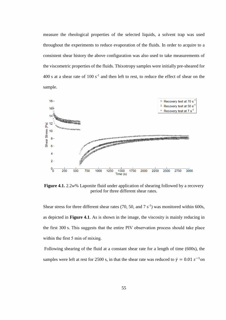
55
measure the rheological properties of the selected liquids, a solvent trap was used
throughout the experiments to reduce evaporation of the fluids. In order to acquire to a
consistent shear history the above configuration was also used to take measurements of
the viscometric properties of the fluids. Thixotropy samples were initially pre-sheared for
400 s at a shear rate of 100 s-1 and then left to rest, to reduce the effect of shear on the
sample.
Figure 4.1. 2.2w% Laponite fluid under application of shearing followed by a recovery
period for three different shear rates.
Shear stress for three different shear rates (70, 50, and 7 s-1) was monitored within 600s,
as depicted in Figure 4.1. As is shown in the image, the viscosity is mainly reducing in
the first 300 s. This suggests that the entire PIV observation process should take place
within the first 5 min of mixing.
Following shearing of the fluid at a constant shear rate for a length of time (600s), the
samples were left at rest for 2500 s, in that the shear rate was reduced to �� = 0.01 𝑠−1on
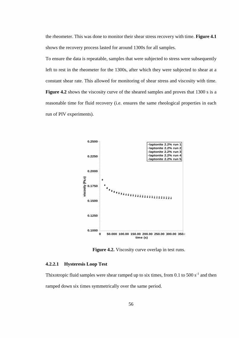
56
the rheometer. This was done to monitor their shear stress recovery with time. Figure 4.1
shows the recovery process lasted for around 1300s for all samples.
To ensure the data is repeatable, samples that were subjected to stress were subsequently
left to rest in the rheometer for the 1300s, after which they were subjected to shear at a
constant shear rate. This allowed for monitoring of shear stress and viscosity with time.
Figure 4.2 shows the viscosity curve of the sheared samples and proves that 1300 s is a
reasonable time for fluid recovery (i.e. ensures the same rheological properties in each
run of PIV experiments).
Figure 4.2. Viscosity curve overlap in test runs.
4.2.2.1 Hysteresis Loop Test
Thixotropic fluid samples were shear ramped up to six times, from 0.1 to 500 s-1 and then
ramped down six times symmetrically over the same period.
0 50.000 100.00 150.00 200.00 250.00 300.00 350.00
time (s)
0.1000
0.1250
0.1500
0.1750
0.2000
0.2250
0.2500
visc
osi
ty (
Pa.
s)
laptonite 2.2% run 1
laptonite 2.2% run 2
laptonite 2.2% run 3
laptonite 2.2% run 4
laptonite 2.2% run 5
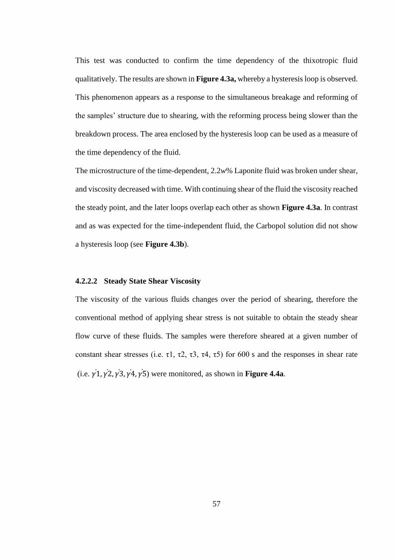
57
This test was conducted to confirm the time dependency of the thixotropic fluid
qualitatively. The results are shown in Figure 4.3a, whereby a hysteresis loop is observed.
This phenomenon appears as a response to the simultaneous breakage and reforming of
the samples’ structure due to shearing, with the reforming process being slower than the
breakdown process. The area enclosed by the hysteresis loop can be used as a measure of
the time dependency of the fluid.
The microstructure of the time-dependent, 2.2w% Laponite fluid was broken under shear,
and viscosity decreased with time. With continuing shear of the fluid the viscosity reached
the steady point, and the later loops overlap each other as shown Figure 4.3a. In contrast
and as was expected for the time-independent fluid, the Carbopol solution did not show
a hysteresis loop (see Figure 4.3b).
4.2.2.2 Steady State Shear Viscosity
The viscosity of the various fluids changes over the period of shearing, therefore the
conventional method of applying shear stress is not suitable to obtain the steady shear
flow curve of these fluids. The samples were therefore sheared at a given number of
constant shear stresses (i.e. τ1, τ2, τ3, τ4, τ5) for 600 s and the responses in shear rate
(i.e. 𝛾1, 𝛾2, 𝛾3, 𝛾4, 𝛾5) were monitored, as shown in Figure 4.4a.
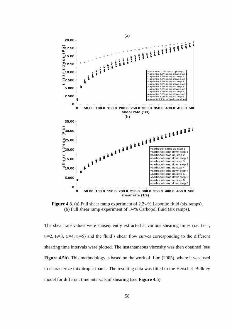
58
(a)
(b)
Figure 4.3. (a) Full shear ramp experiment of 2.2w% Laponite fluid (six ramps),
(b) Full shear ramp experiment of 1w% Carbopol fluid (six ramps).
The shear rate values were subsequently extracted at various shearing times (i.e. t1=1,
t2=2, t3=3, t4=4, t5=5) and the fluid’s shear flow curves corresponding to the different
shearing time intervals were plotted. The instantaneous viscosity was then obtained (see
Figure 4.5b). This methodology is based on the work of Lim (2005), where it was used
to characterize thixotropic foams. The resulting data was fitted to the Herschel–Bulkley
model for different time intervals of shearing (see Figure 4.5):
0 50.00 100.0 150.0 200.0 250.0 300.0 350.0 400.0 450.0 500.0
shear rate (1/s)
0
2.500
5.000
7.500
10.00
12.50
15.00
17.50
20.00
sh
ea
r s
tre
ss
(P
a)
laptonite 2.2% ramp up step 1
laptonite 2.2% ramp down step 1
laptonite 2.2% ramp up step 2
laptonite 2.2% ramp down step 2
laptonite 2.2% ramp up step 3
laptonite 2.2% ramp down step 3
laptonite 2.2% ramp up step 4
laptonite 2.2% ramp down step 4
laptonite 2.2% ramp up step 5
laptonite 2.2% ramp down step 5
laptonite 2.2% ramp up step 6
laptonite2.2% ramp down step 6
0 50.00 100.0 150.0 200.0 250.0 300.0 350.0 400.0 450.0 500.0
shear rate (1/s)
0
5.000
10.00
15.00
20.00
25.00
30.00
35.00
sh
ea
r s
tre
ss
(P
a)
carbopol ramp up step 1
carbopol ramp down step 1
carbopol ramp up step 2
carbopol ramp down step 2
carbopol ramp up step 3
carbopol ramp down step 3
carbopol ramp up step 4
carbopol ramp down step 4
carbopol ramp up step 5
carbopol ramp down step 5
carbopol ramp up step 6
carbopol ramp down step 6
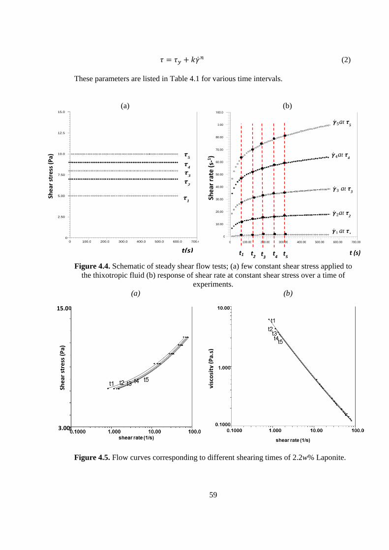
59
𝜏 = 𝜏𝑦 + 𝑘��𝑛 (2)
These parameters are listed in Table 4.1 for various time intervals.
(a) (b)
Figure 4.4. Schematic of steady shear flow tests; (a) few constant shear stress applied to
the thixotropic fluid (b) response of shear rate at constant shear stress over a time of
experiments.
(a) (b)
Figure 4.5. Flow curves corresponding to different shearing times of 2.2w% Laponite.
0 100.0 200.0 300.0 400.0 500.0 600.0 700.0 0
2.50
5.00
7.50
10.0
12.5
15.0
τ1
τ2
τ3
τ4
τ5
t(s)
τ (Pa)
0 100.00 200.00 300.00 400.00 500.00 600.00 700.00 0
10.00
20.00
30.00
40.00
50.00
60.00
70.00
80.00
90.00
100.0
t (s) t1 t2 t
3 t
4 t
5
(1/S)
1 at τ
1
2at τ2
3 at τ3
4at τ4
5at τ5
Shea
r ra
te (
s-1)
She
ar s
tre
ss (
Pa)
Sh
ear
str
ess
(P
a)
15.0 3.00
visc
osi
ty (
Pa.
s)
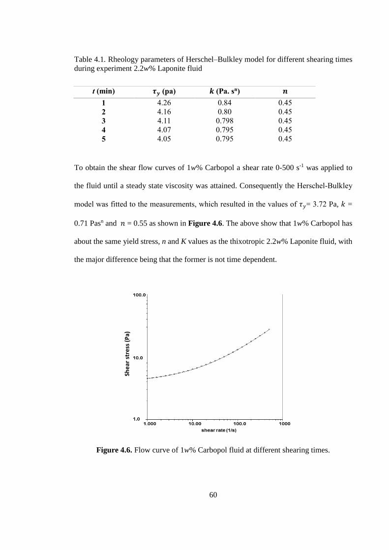
60
Table 4.1. Rheology parameters of Herschel–Bulkley model for different shearing times
during experiment 2.2w% Laponite fluid
To obtain the shear flow curves of 1w% Carbopol a shear rate 0-500 s-1 was applied to
the fluid until a steady state viscosity was attained. Consequently the Herschel-Bulkley
model was fitted to the measurements, which resulted in the values of 𝜏𝑦= 3.72 Pa, 𝑘 =
0.71 Pasn and 𝑛 = 0.55 as shown in Figure 4.6. The above show that 1w% Carbopol has
about the same yield stress, n and K values as the thixotropic 2.2w% Laponite fluid, with
the major difference being that the former is not time dependent.
Figure 4.6. Flow curve of 1w% Carbopol fluid at different shearing times.
t (min) 𝝉𝒚 (pa) 𝒌 (Pa. sn) 𝒏 1 4.26 0.84 0.45 2 4.16 0.80 0.45 3 4.11 0.798 0.45 4 4.07 0.795 0.45 5 4.05 0.795 0.45
She
ar s
tre
ss (
Pa)
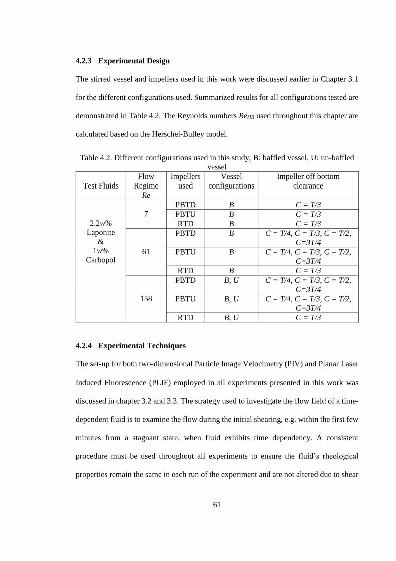
61
4.2.3 Experimental Design
The stirred vessel and impellers used in this work were discussed earlier in Chapter 3.1
for the different configurations used. Summarized results for all configurations tested are
demonstrated in Table 4.2. The Reynolds numbers ReHB used throughout this chapter are
calculated based on the Herschel-Bulley model.
Table 4.2. Different configurations used in this study; B: baffled vessel, U: un-baffled
vessel
Test Fluids
Flow
Regime
Re
Impellers
used
Vessel
configurations
Impeller off bottom
clearance
2.2w%
Laponite
&
1w%
Carbopol
7
PBTD B C = T/3
PBTU B C = T/3
RTD B C = T/3
61
PBTD B C = T/4, C = T/3, C = T/2,
C=3T/4
PBTU B C = T/4, C = T/3, C = T/2,
C=3T/4
RTD B C = T/3
158
PBTD B, U C = T/4, C = T/3, C = T/2,
C=3T/4
PBTU B, U C = T/4, C = T/3, C = T/2,
C=3T/4
RTD B, U C = T/3
4.2.4 Experimental Techniques
The set-up for both two-dimensional Particle Image Velocimetry (PIV) and Planar Laser
Induced Fluorescence (PLIF) employed in all experiments presented in this work was
discussed in chapter 3.2 and 3.3. The strategy used to investigate the flow field of a time-
dependent fluid is to examine the flow during the initial shearing, e.g. within the first few
minutes from a stagnant state, when fluid exhibits time dependency. A consistent
procedure must be used throughout all experiments to ensure the fluid’s rheological
properties remain the same in each run of the experiment and are not altered due to shear
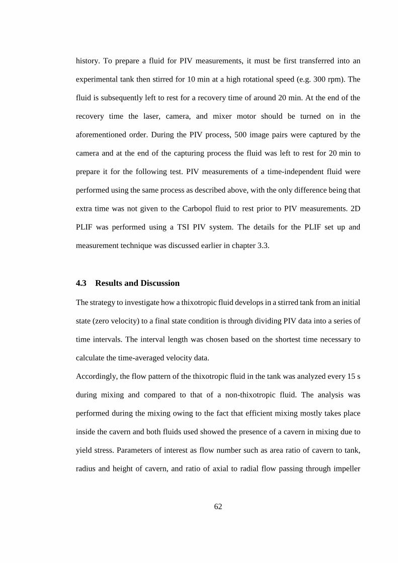
62
history. To prepare a fluid for PIV measurements, it must be first transferred into an
experimental tank then stirred for 10 min at a high rotational speed (e.g. 300 rpm). The
fluid is subsequently left to rest for a recovery time of around 20 min. At the end of the
recovery time the laser, camera, and mixer motor should be turned on in the
aforementioned order. During the PIV process, 500 image pairs were captured by the
camera and at the end of the capturing process the fluid was left to rest for 20 min to
prepare it for the following test. PIV measurements of a time-independent fluid were
performed using the same process as described above, with the only difference being that
extra time was not given to the Carbopol fluid to rest prior to PIV measurements. 2D
PLIF was performed using a TSI PIV system. The details for the PLIF set up and
measurement technique was discussed earlier in chapter 3.3.
4.3 Results and Discussion
The strategy to investigate how a thixotropic fluid develops in a stirred tank from an initial
state (zero velocity) to a final state condition is through dividing PIV data into a series of
time intervals. The interval length was chosen based on the shortest time necessary to
calculate the time-averaged velocity data.
Accordingly, the flow pattern of the thixotropic fluid in the tank was analyzed every 15 s
during mixing and compared to that of a non-thixotropic fluid. The analysis was
performed during the mixing owing to the fact that efficient mixing mostly takes place
inside the cavern and both fluids used showed the presence of a cavern in mixing due to
yield stress. Parameters of interest as flow number such as area ratio of cavern to tank,
radius and height of cavern, and ratio of axial to radial flow passing through impeller
63
were determined from the time-averaged velocity data during each shearing time. It
should be noted that a negative value of flow numbers means the flow leaves the plane of
the impeller.
The PLIF visualization technique was employed to help characterize the mixing
efficiency in terms of cavern growth and size as well as measure the time required for the
fluid inside cavern to become fully mixed.
2D normalized velocity contour plots for the three impeller configurations were
determined under three different flow regimes (ReHB = 7, ReHB = 61, ReHB = 158) and
three time intervals (t1 = 0-15 s, t2 =125-139 s, t3 = 261-277 s) during mixing. The PBT
impeller in both UP and DP modes and the RTD impeller make it possible to investigate
in more detail the efficiency of axial and radial flow discharge of the thixotropic fluid.
Results are presented and discussed for each Re number.
4.3.1 Flow Fields
4.3.1.1 Re = 158
A primary anti-clockwise loop was observed in the PBTD impeller configuration in the
first 15 s of stirring that appeared to extend both vertically and horizontally due to the
reduction of viscosity taking place from time t1 to t3 (see Figure 4.7). The flow was
induced vertically from above the impeller at t1 and mostly to the left of the impeller, at
an angle of 45◦ with respect to the downward direction. Hence the flow discharge is found
to be mostly axially, with the ratio of axial to radial pumping being Qa/Qr = 3.10 (Table
4.3). Couerbe et al. (2008) observed a similar value for the same fluid mixed by a Mixel
TT impeller at N = 8 s-1 whereby what was determined was the flow is in the transition
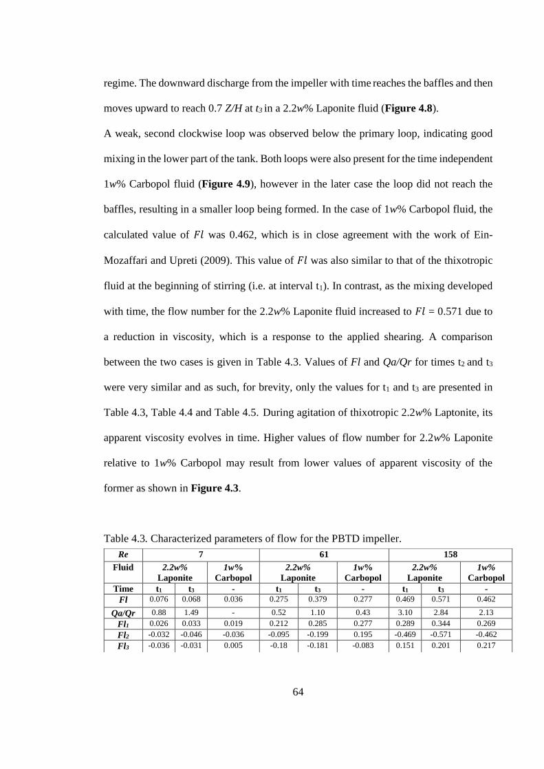
64
regime. The downward discharge from the impeller with time reaches the baffles and then
moves upward to reach 0.7 Z/H at t3 in a 2.2w% Laponite fluid (Figure 4.8).
A weak, second clockwise loop was observed below the primary loop, indicating good
mixing in the lower part of the tank. Both loops were also present for the time independent
1w% Carbopol fluid (Figure 4.9), however in the later case the loop did not reach the
baffles, resulting in a smaller loop being formed. In the case of 1w% Carbopol fluid, the
calculated value of 𝐹𝑙 was 0.462, which is in close agreement with the work of Ein-
Mozaffari and Upreti (2009). This value of 𝐹𝑙 was also similar to that of the thixotropic
fluid at the beginning of stirring (i.e. at interval t1). In contrast, as the mixing developed
with time, the flow number for the 2.2w% Laponite fluid increased to 𝐹𝑙 = 0.571 due to
a reduction in viscosity, which is a response to the applied shearing. A comparison
between the two cases is given in Table 4.3. Values of Fl and Qa/Qr for times t2 and t3
were very similar and as such, for brevity, only the values for t1 and t3 are presented in
Table 4.3, Table 4.4 and Table 4.5. During agitation of thixotropic 2.2w% Laptonite, its
apparent viscosity evolves in time. Higher values of flow number for 2.2w% Laponite
relative to 1w% Carbopol may result from lower values of apparent viscosity of the
former as shown in Figure 4.3.
Table 4.3. Characterized parameters of flow for the PBTD impeller.
Re 7 61 158
Fluid 2.2w%
Laponite
1w%
Carbopol
2.2w%
Laponite
1w%
Carbopol
2.2w%
Laponite
1w%
Carbopol
Time t1 t3 - t1 t3 - t1 t3 -
Fl 0.076 0.068 0.036 0.275 0.379 0.277 0.469 0.571 0.462
Qa/Qr 0.88 1.49 - 0.52 1.10 0.43 3.10 2.84 2.13
Fl1 0.026 0.033 0.019 0.212 0.285 0.277 0.289 0.344 0.269
Fl2 -0.032 -0.046 -0.036 -0.095 -0.199 0.195 -0.469 -0.571 -0.462
Fl3 -0.036 -0.031 0.005 -0.18 -0.181 -0.083 0.151 0.201 0.217
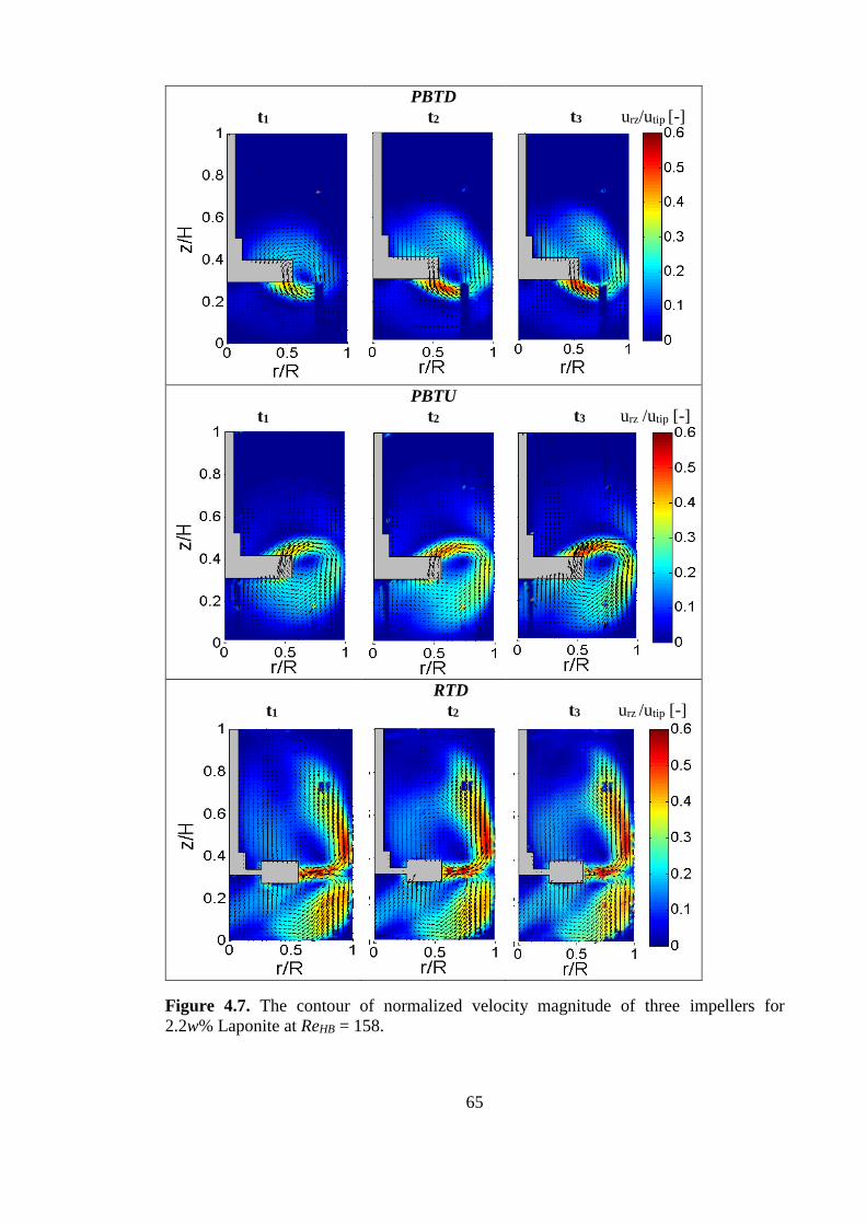
65
Figure 4.7. The contour of normalized velocity magnitude of three impellers for
2.2w% Laponite at ReHB = 158.
t1
PBTD
t2
t3 urz/utip [-]
t1
PBTU
t2
t3 urz /utip [-]
t1
RTD
t2
t3 urz /utip [-]
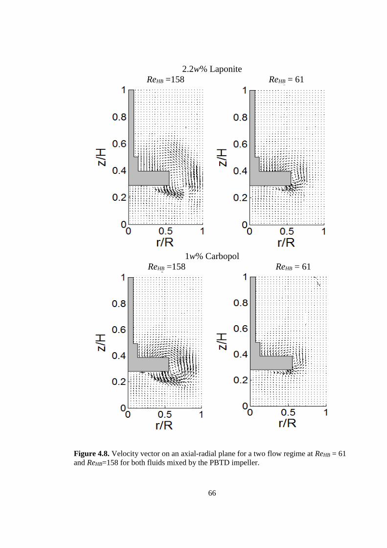
66
2.2w% Laponite
ReHB =158 ReHB = 61
1w% Carbopol
ReHB =158 ReHB = 61
Figure 4.8. Velocity vector on an axial-radial plane for a two flow regime at ReHB = 61
and ReHB=158 for both fluids mixed by the PBTD impeller.
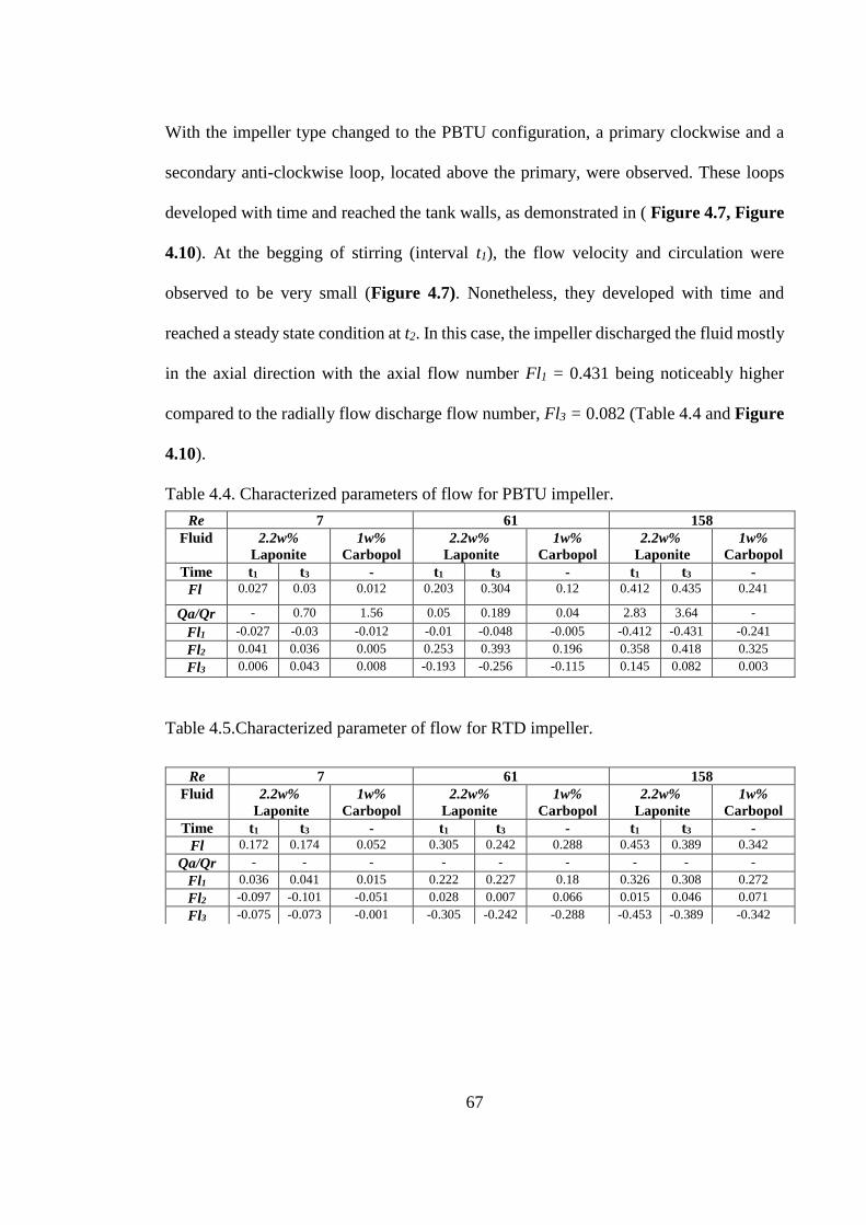
67
With the impeller type changed to the PBTU configuration, a primary clockwise and a
secondary anti-clockwise loop, located above the primary, were observed. These loops
developed with time and reached the tank walls, as demonstrated in ( Figure 4.7, Figure
4.10). At the begging of stirring (interval t1), the flow velocity and circulation were
observed to be very small (Figure 4.7). Nonetheless, they developed with time and
reached a steady state condition at t2. In this case, the impeller discharged the fluid mostly
in the axial direction with the axial flow number Fl1 = 0.431 being noticeably higher
compared to the radially flow discharge flow number, Fl3 = 0.082 (Table 4.4 and Figure
4.10).
Table 4.4. Characterized parameters of flow for PBTU impeller.
Table 4.5.Characterized parameter of flow for RTD impeller.
Re 7 61 158
Fluid 2.2w%
Laponite
1w%
Carbopol
2.2w%
Laponite
1w%
Carbopol
2.2w%
Laponite
1w%
Carbopol
Time t1 t3 - t1 t3 - t1 t3 -
Fl 0.027 0.03 0.012 0.203 0.304 0.12 0.412 0.435 0.241
Qa/Qr - 0.70 1.56 0.05 0.189 0.04 2.83 3.64 -
Fl1 -0.027 -0.03 -0.012 -0.01 -0.048 -0.005 -0.412 -0.431 -0.241
Fl2 0.041 0.036 0.005 0.253 0.393 0.196 0.358 0.418 0.325
Fl3 0.006 0.043 0.008 -0.193 -0.256 -0.115 0.145 0.082 0.003
Re 7 61 158
Fluid 2.2w%
Laponite
1w%
Carbopol
2.2w%
Laponite
1w%
Carbopol
2.2w%
Laponite
1w%
Carbopol
Time t1 t3 - t1 t3 - t1 t3 -
Fl 0.172 0.174 0.052 0.305 0.242 0.288 0.453 0.389 0.342
Qa/Qr - - - - - - - - -
Fl1 0.036 0.041 0.015 0.222 0.227 0.18 0.326 0.308 0.272
Fl2 -0.097 -0.101 -0.051 0.028 0.007 0.066 0.015 0.046 0.071
Fl3 -0.075 -0.073 -0.001 -0.305 -0.242 -0.288 -0.453 -0.389 -0.342
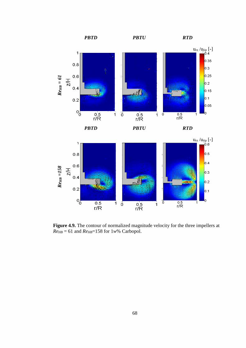
68
PBTD PBTU RTD
Re H
B =
61
urz /utip [-]
PBTD PBTU RTD
Re H
B =
158
urz /utip [-]
Figure 4.9. The contour of normalized magnitude velocity for the three impellers at
ReHB = 61 and ReHB=158 for 1w% Carbopol.
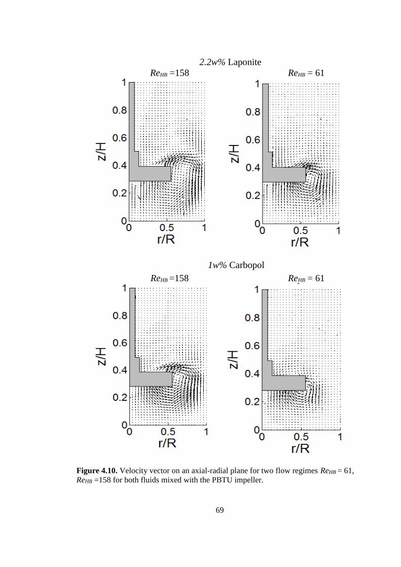
69
2.2w% Laponite
ReHB =158 ReHB = 61
1w% Carbopol
ReHB =158 ReHB = 61
Figure 4.10. Velocity vector on an axial-radial plane for two flow regimes ReHB = 61,
ReHB =158 for both fluids mixed with the PBTU impeller.
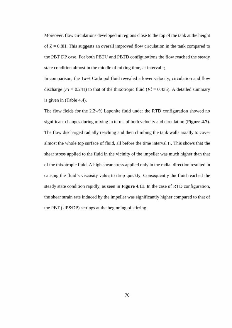
70
Moreover, flow circulations developed in regions close to the top of the tank at the height
of Z = 0.8H. This suggests an overall improved flow circulation in the tank compared to
the PBT DP case. For both PBTU and PBTD configurations the flow reached the steady
state condition almost in the middle of mixing time, at interval t2.
In comparison, the 1w% Carbopol fluid revealed a lower velocity, circulation and flow
discharge (𝐹𝑙 = 0.241) to that of the thixotropic fluid (𝐹𝑙 = 0.435). A detailed summary
is given in (Table 4.4).
The flow fields for the 2.2w% Laponite fluid under the RTD configuration showed no
significant changes during mixing in terms of both velocity and circulation (Figure 4.7).
The flow discharged radially reaching and then climbing the tank walls axially to cover
almost the whole top surface of fluid, all before the time interval t1. This shows that the
shear stress applied to the fluid in the vicinity of the impeller was much higher than that
of the thixotropic fluid. A high shear stress applied only in the radial direction resulted in
causing the fluid’s viscosity value to drop quickly. Consequently the fluid reached the
steady state condition rapidly, as seen in Figure 4.11. In the case of RTD configuration,
the shear strain rate induced by the impeller was significantly higher compared to that of
the PBT (UP&DP) settings at the beginning of stirring.
71
Figure 4.11. Contour of shear strain rate plot for 2.2w% Laponite (at t1 and t3) and
1w% Carbopol fluid.
t1 2.2w% Laponite t3 1w% Carbopol
RT
D
t1 2.2w% Laponite t3 1w% Carbopol
PB
TD
t1 2.2w% Laponite t3 1w% Carbopol
PB
TU
72
4.3.1.2 Re = 61
shows the velocity fields for a reduced mixing speed at ReHB = 61. The graph still shows
presence of both the primary and secondary loops under the three different impeller
configurations, however their velocity and circulation loop were reduced in terms of both
value and size respectively, compared to the previous cases. The flow fields from the PIV
data show the formation of a cavern that grows over the course of mixing, as shown in
Figure 4.12. The flow was discharged more radially from the PBT impellers (UP&DP)
than in the previous case (ReHB = 158), causing a noticeable reduction in the ratio of axial
to radial pumping Qa/Qr as seen in Table 4.3 and Table 4.4. This is in-line with the
findings of Couerbe et al. (2008), Chung (2008) who observed a reduction of axial
pumping in an axial impeller configuration for a thixotropic fluid and Newtonian fluid
respectively at lower Reynold number. The 𝐹𝑙 and Qa/Qr values exhibited the same
increasing trend as seen before with time of stirring. Under the PBT configuration
(DP&UP) both the 2.2 w% Laponite and the 1.5w%Carbopol fluids showed very low Fl
and Qa/Qr values at the beginning of stirring t1 (see Table 4.3, Table 4.4 and Table 4.5).
The pumping capacity (Fl) of the thixtropic fluid increased with time and the impeller
started to pump in the axial direction more than 50% (Qa/Qr) than the beginning of
mixing (Table 4.3, Table 4.4, and Figure 4.12).
4.3.1.3 Re = 7
Further reduction of mixing speed brings the flow condition to the laminar regime at
ReHB = 7. As can be seen in Figure 4.13 and Tables 4.3 to 4.5, the flow pumping capacity
for the 2.2 w% Laponite fluid remained comparitevely the same from t1 to t3, being
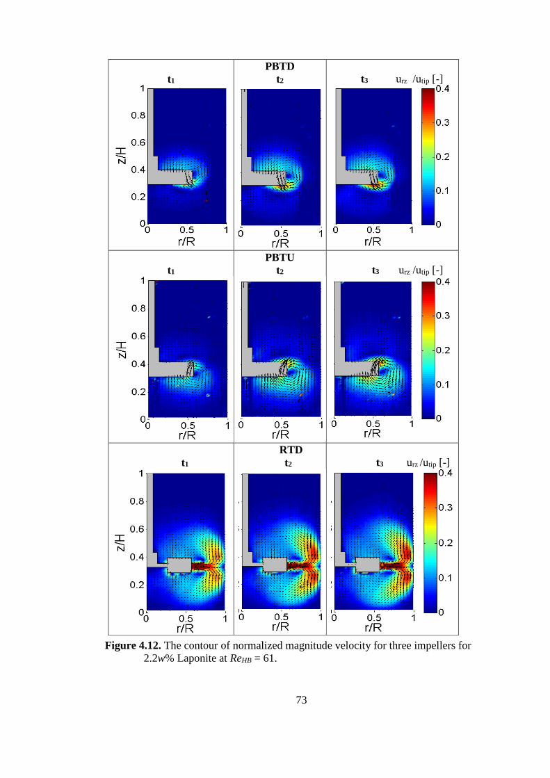
73
Figure 4.12. The contour of normalized magnitude velocity for three impellers for
2.2w% Laponite at ReHB = 61.
t1
PBTD
t2
t3 urz /utip [-]
t1
PBTU
t2
t3 urz /utip [-]
t1
RTD
t2
t3 urz /utip [-]
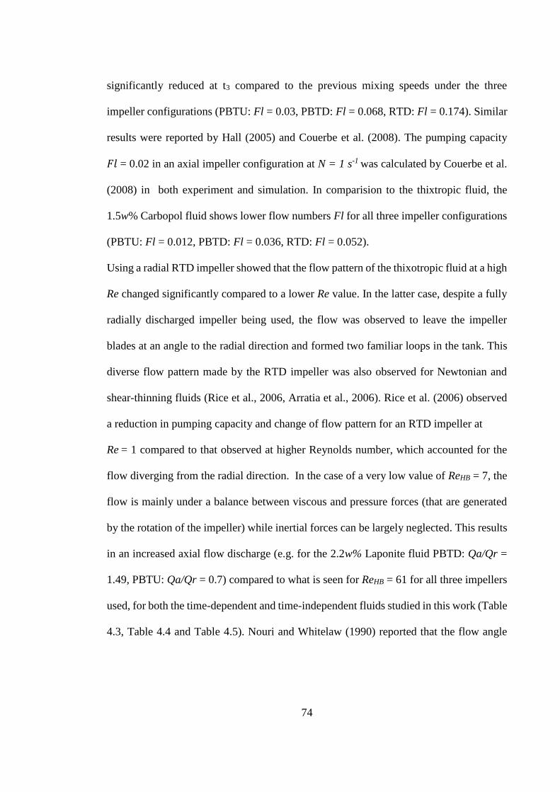
74
significantly reduced at t3 compared to the previous mixing speeds under the three
impeller configurations (PBTU: Fl = 0.03, PBTD: Fl = 0.068, RTD: Fl = 0.174). Similar
results were reported by Hall (2005) and Couerbe et al. (2008). The pumping capacity
𝐹𝑙 = 0.02 in an axial impeller configuration at N = 1 s-1 was calculated by Couerbe et al.
(2008) in both experiment and simulation. In comparision to the thixtropic fluid, the
1.5w% Carbopol fluid shows lower flow numbers Fl for all three impeller configurations
(PBTU: Fl = 0.012, PBTD: Fl = 0.036, RTD: Fl = 0.052).
Using a radial RTD impeller showed that the flow pattern of the thixotropic fluid at a high
Re changed significantly compared to a lower Re value. In the latter case, despite a fully
radially discharged impeller being used, the flow was observed to leave the impeller
blades at an angle to the radial direction and formed two familiar loops in the tank. This
diverse flow pattern made by the RTD impeller was also observed for Newtonian and
shear-thinning fluids (Rice et al., 2006, Arratia et al., 2006). Rice et al. (2006) observed
a reduction in pumping capacity and change of flow pattern for an RTD impeller at
Re = 1 compared to that observed at higher Reynolds number, which accounted for the
flow diverging from the radial direction. In the case of a very low value of ReHB = 7, the
flow is mainly under a balance between viscous and pressure forces (that are generated
by the rotation of the impeller) while inertial forces can be largely neglected. This results
in an increased axial flow discharge (e.g. for the 2.2w% Laponite fluid PBTD: Qa/Qr =
1.49, PBTU: Qa/Qr = 0.7) compared to what is seen for ReHB = 61 for all three impellers
used, for both the time-dependent and time-independent fluids studied in this work (Table
4.3, Table 4.4 and Table 4.5). Nouri and Whitelaw (1990) reported that the flow angle
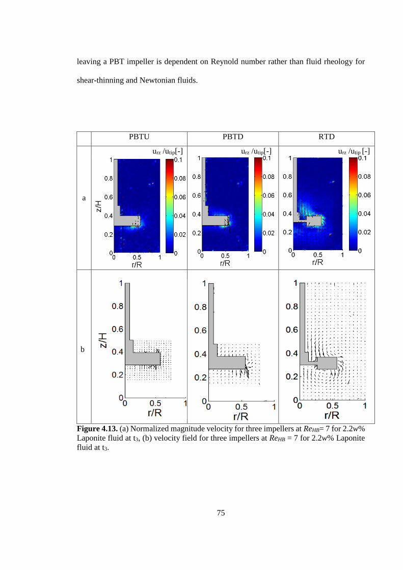
75
leaving a PBT impeller is dependent on Reynold number rather than fluid rheology for
shear-thinning and Newtonian fluids.
PBTU PBTD RTD
urz /utip[-] urz /utip[-] urz /utip [-]
a
b
Figure 4.13. (a) Normalized magnitude velocity for three impellers at ReHB= 7 for 2.2w%
Laponite fluid at t3, (b) velocity field for three impellers at ReHB = 7 for 2.2w% Laponite
fluid at t3.
76
4.3.2 Cavern Growth
Due to the thixotropic fluids having a yield stress, a cavern is formed inside the tank at
low velocities (i.e. low mixing speeds). Since all of the mixings takes place inside the
cavern area, measurements of cavern size would provide valuable information about the
extent of mixing of the fluid. A velocity threshold of uuv = 0.01utip, as proposed by
Adams and Barigou (2007), was used in this work to define the cavern boundary and
subsequently obtain the cavern size. Cavern diameter (Dc), cavern height (Hc) and the
ratio of cavern area to tank area (AC/AT) are the parameters that were used to characterize
the cavern in these fluids.
(a) (b)
Figure 4.14. The changes of normalized cavern area % for the thixotropic fluid as a
function of time for (a) ReHB= 158 and (b) ReHB = 61.
Variations of cavern size AC/AT with time for ReHB = 61 and ReHB = 158 are presented in
Figure 4.14. The data shows that the cavern grows radially (Dc) at ReHB =158 under the
PBT (UP & DP) impeller configuration and reached the tank walls within t = 50 s
(Figure 4.15a). The cavern then expanded axially (Hc) and reached a height of Z = 0.86
0
20
40
60
80
100
120
0 50 100 150 200 250 300
AC/A
T%
Time(s)
PBTU
RTD
PBTD
0
20
40
60
80
100
0 100 200 300
AC
/AT
%
Time(s)
PBTDPBTURTD
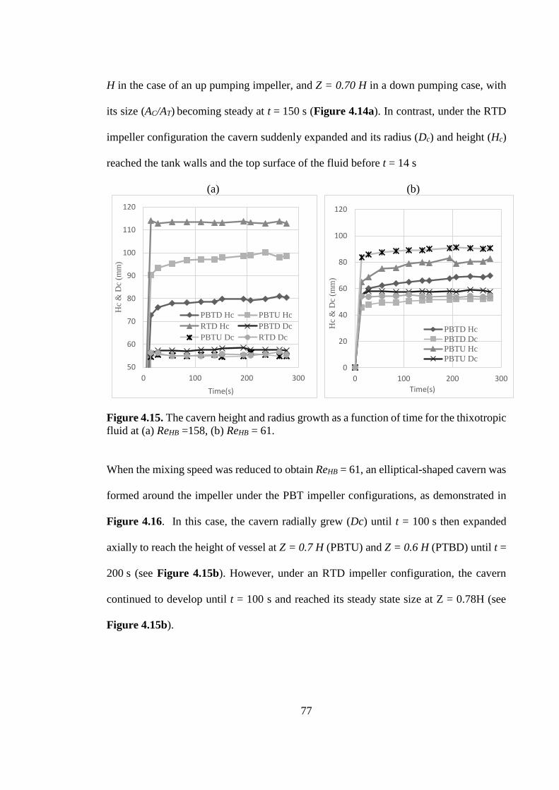
77
H in the case of an up pumping impeller, and Z = 0.70 H in a down pumping case, with
its size (AC/AT) becoming steady at t = 150 s (Figure 4.14a). In contrast, under the RTD
impeller configuration the cavern suddenly expanded and its radius (Dc) and height (Hc)
reached the tank walls and the top surface of the fluid before t = 14 s
(a) (b)
Figure 4.15. The cavern height and radius growth as a function of time for the thixotropic
fluid at (a) ReHB =158, (b) ReHB = 61.
When the mixing speed was reduced to obtain ReHB = 61, an elliptical-shaped cavern was
formed around the impeller under the PBT impeller configurations, as demonstrated in
Figure 4.16. In this case, the cavern radially grew (Dc) until t = 100 s then expanded
axially to reach the height of vessel at Z = 0.7 H (PBTU) and Z = 0.6 H (PTBD) until t =
200 s (see Figure 4.15b). However, under an RTD impeller configuration, the cavern
continued to develop until t = 100 s and reached its steady state size at Z = 0.78H (see
Figure 4.15b).
50
60
70
80
90
100
110
120
0 100 200 300
Hc
& D
c (m
m)
Time(s)
PBTD Hc PBTU Hc
RTD Hc PBTD Dc
PBTU Dc RTD Dc
0
20
40
60
80
100
120
0 100 200 300
Hc
& D
c (m
m)
Time(s)
PBTD Hc
PBTD Dc
PBTU Hc
PBTU Dc
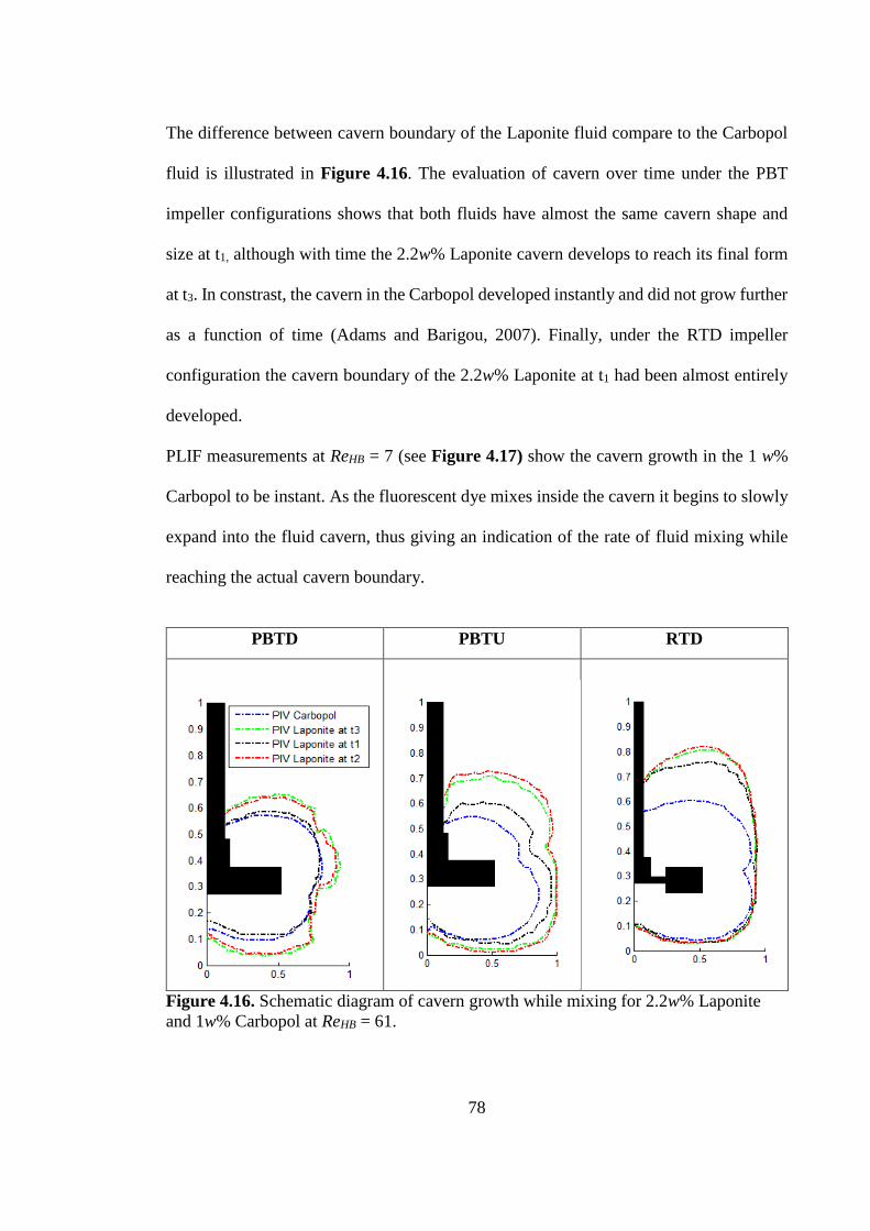
78
The difference between cavern boundary of the Laponite fluid compare to the Carbopol
fluid is illustrated in Figure 4.16. The evaluation of cavern over time under the PBT
impeller configurations shows that both fluids have almost the same cavern shape and
size at t1, although with time the 2.2w% Laponite cavern develops to reach its final form
at t3. In constrast, the cavern in the Carbopol developed instantly and did not grow further
as a function of time (Adams and Barigou, 2007). Finally, under the RTD impeller
configuration the cavern boundary of the 2.2w% Laponite at t1 had been almost entirely
developed.
PLIF measurements at ReHB = 7 (see Figure 4.17) show the cavern growth in the 1 w%
Carbopol to be instant. As the fluorescent dye mixes inside the cavern it begins to slowly
expand into the fluid cavern, thus giving an indication of the rate of fluid mixing while
reaching the actual cavern boundary.
PBTD PBTU RTD
Figure 4.16. Schematic diagram of cavern growth while mixing for 2.2w% Laponite
and 1w% Carbopol at ReHB = 61.
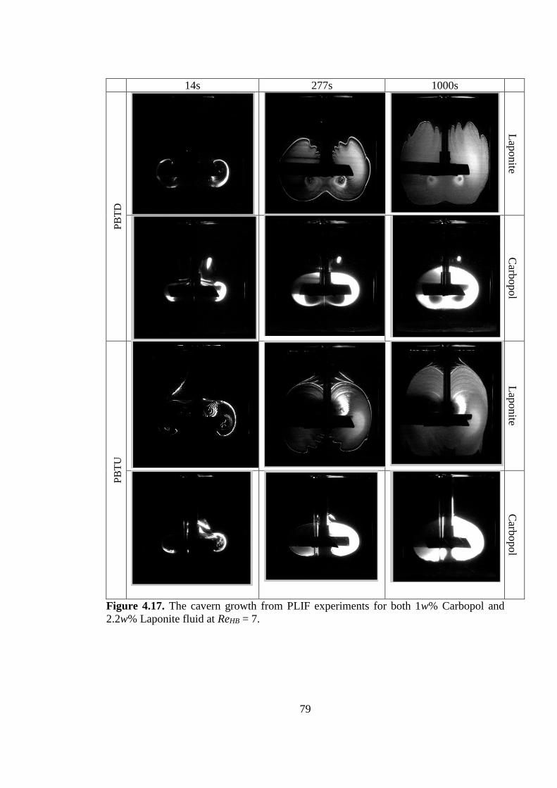
79
14s 277s 1000s
PB
TD
PB
TD
Lap
onite
Carb
opol
PB
TU
PB
TU
Lap
onite
Carb
opol
Figure 4.17. The cavern growth from PLIF experiments for both 1w% Carbopol and
2.2w% Laponite fluid at ReHB = 7.
80
The cavern boundary in the Laponite fluid started to develop very gradually until it
stopped growing at t = 1000 s, with the fluorescent dye being found to still be
inhomogeneously mixed inside the cavern as shown in Figure 4.17. The difference in
cavern shape and development pattern for the thixotropic and viscoplastic fluids indicate
that for the former a significant axial growth was also followed by a radial growth,
resulting in an irregular cavern boundary.
4.3.3 Effect of Non-standard Configurations
4.3.3.1 Un-baffled Vessel
Conventionally, baffles are used to prevent solid body rotation of fluid in a tank, so as to
enhance mixing performance. In Newtonian fluids, especially in a turbulent regime, it is
desirable to use baffles in order to improve axial circulation and prevent the formation of
the free vortex at the surface of fluid as well as reducing mixing time (Armenante et al.,
1997, Chung, 2008). However, this does not necessary apply for Non-Newtonian fluids;
Hirata and Aoshima (1996) observed that baffles have a negative effect on the cavern size
growth in the case of viscoplastic fluids.
Figure 4.18 shows a variation of Power number as a function of Reynolds number in the
cases of baffled and un-baffled configurations with RTD impeller for both a viscoplastic
fluid and a Newtonian fluid.
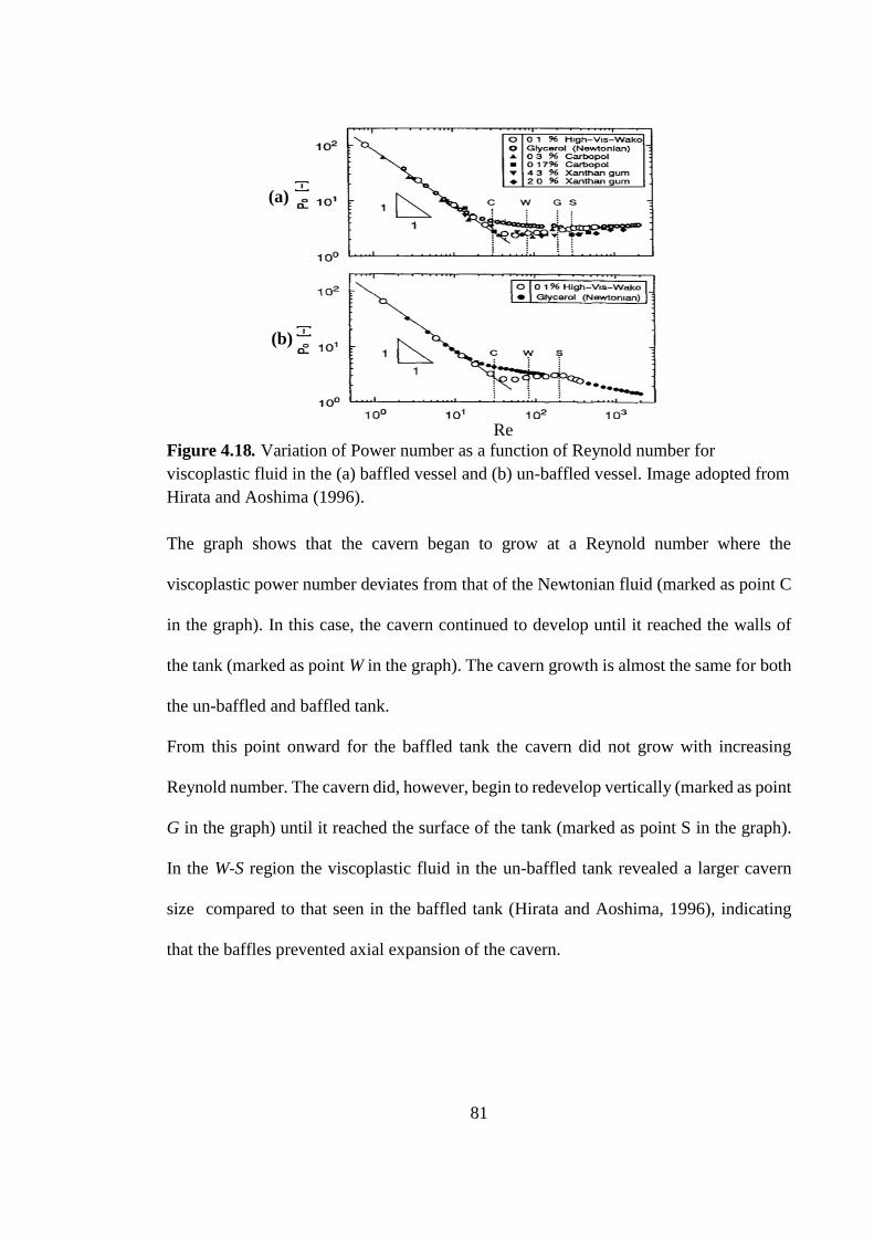
81
Re
Figure 4.18. Variation of Power number as a function of Reynold number for
viscoplastic fluid in the (a) baffled vessel and (b) un-baffled vessel. Image adopted from
Hirata and Aoshima (1996).
The graph shows that the cavern began to grow at a Reynold number where the
viscoplastic power number deviates from that of the Newtonian fluid (marked as point C
in the graph). In this case, the cavern continued to develop until it reached the walls of
the tank (marked as point W in the graph). The cavern growth is almost the same for both
the un-baffled and baffled tank.
From this point onward for the baffled tank the cavern did not grow with increasing
Reynold number. The cavern did, however, begin to redevelop vertically (marked as point
G in the graph) until it reached the surface of the tank (marked as point S in the graph).
In the W-S region the viscoplastic fluid in the un-baffled tank revealed a larger cavern
size compared to that seen in the baffled tank (Hirata and Aoshima, 1996), indicating
that the baffles prevented axial expansion of the cavern.
(a)
(b)
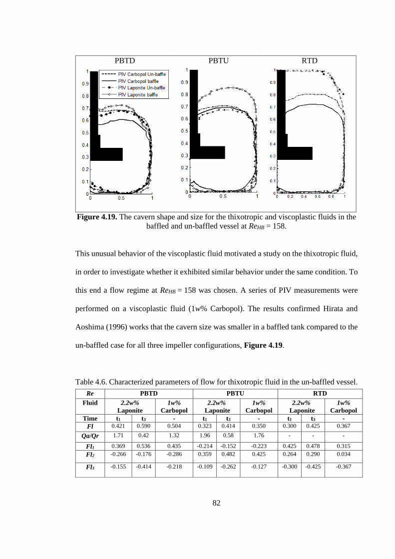
82
PBTD PBTU RTD
Figure 4.19. The cavern shape and size for the thixotropic and viscoplastic fluids in the
baffled and un-baffled vessel at ReHB = 158.
This unusual behavior of the viscoplastic fluid motivated a study on the thixotropic fluid,
in order to investigate whether it exhibited similar behavior under the same condition. To
this end a flow regime at ReHB = 158 was chosen. A series of PIV measurements were
performed on a viscoplastic fluid (1w% Carbopol). The results confirmed Hirata and
Aoshima (1996) works that the cavern size was smaller in a baffled tank compared to the
un-baffled case for all three impeller configurations, Figure 4.19.
Table 4.6. Characterized parameters of flow for thixotropic fluid in the un-baffled vessel.
Re PBTD PBTU RTD
Fluid 2.2w%
Laponite
1w%
Carbopol
2.2w%
Laponite
1w%
Carbopol
2.2w%
Laponite
1w%
Carbopol
Time t1 t3 - t1 t3 - t1 t3 -
Fl 0.421 0.590 0.504 0.323 0.414 0.350 0.300 0.425 0.367
Qa/Qr 1.71 0.42 1.32 1.96 0.58 1.76 - - -
Fl1 0.369 0.536 0.435 -0.214 -0.152 -0.223 0.425 0.478 0.315
Fl2 -0.266 -0.176 -0.286 0.359 0.482 0.425 0.264 0.290 0.034
Fl3 -0.155 -0.414 -0.218 -0.109 -0.262 -0.127 -0.300 -0.425 -0.367
83
This can be explained by the inability of the fluid to overcome its yield stress due to
momentum losses taking place near the baffles. However, the PIV measurements showed
almost the same flow pattern (qualitatively) under the PBT impellers (UP & DP) in both
of baffled and un-baffled tank (see Figure 4.20). For the un-baffled tank the flow number
has a higher value of 𝐹𝑙 = 0.504 (PBTU) and 𝐹𝑙 = 0.35 (PBTD) than for the baffled tank.
A comparison is given in Table 4.6. Moreover, the radial velocity component along the
axial direction at r = 0.85R in z = 0.3H (Figure 4.21) shows a higher value in the un-
baffled tank under the PBT impeller configurations compared to the baffled case.
However, along the radial direction noticeable difference were not observed in axial and
radial velocities between the baffled and un-baffled tanks (Figure 4.22). Under the RTD
configuration the impeller induced a radial flow, which developed to the side walls of the
tank. Two circulation loops were formed which were observed to be larger in the un-
baffled tank, despite a lower velocity magnitude being observed (Figure 4.20). This,
however, is due to the limitation of the PIV procedure in capturing the tangential velocity
component (the third component normal to the plane of view), which is dominant in the
un-baffled case.
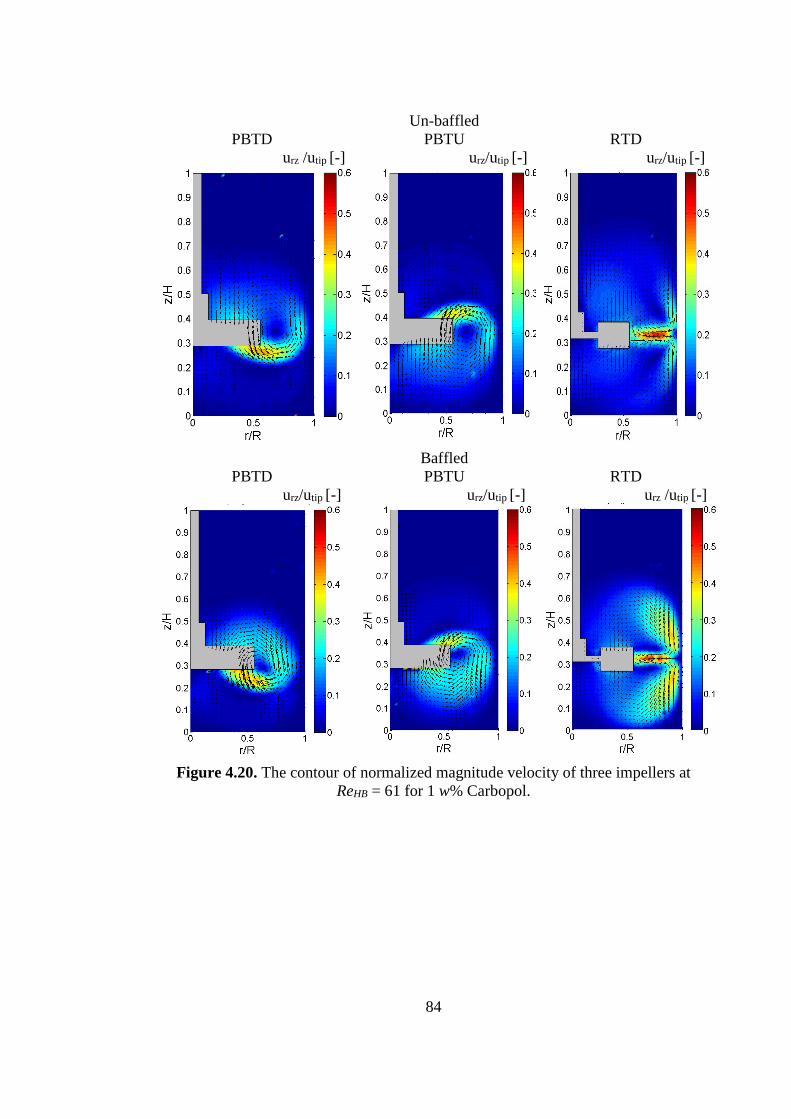
84
PBTD
Un-baffled
PBTU
RTD
urz /utip [-]
urz/utip [-]
urz/utip [-]
PBTD
Baffled
PBTU
RTD
urz/utip [-]
urz/utip [-]
urz /utip [-]
Figure 4.20. The contour of normalized magnitude velocity of three impellers at
ReHB = 61 for 1 w% Carbopol.
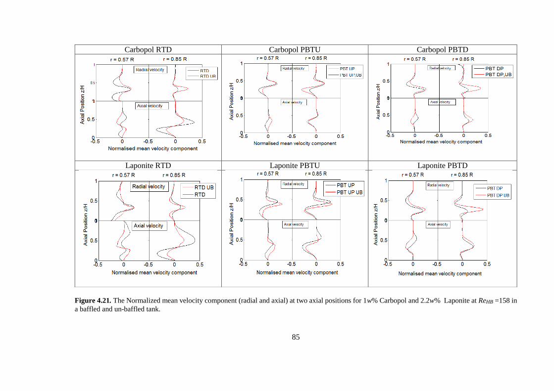
85
Figure 4.21. The Normalized mean velocity component (radial and axial) at two axial positions for 1w% Carbopol and 2.2w% Laponite at ReHB =158 in
a baffled and un-baffled tank.
Carbopol RTD Carbopol PBTU Carbopol PBTD
Laponite RTD Laponite PBTU Laponite PBTD
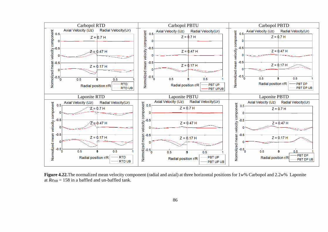
86
Figure 4.22.The normalized mean velocity component (radial and axial) at three horizontal positions for 1w% Carbopol and 2.2w% Laponite
at ReHB = 158 in a baffled and un-baffled tank.
Carbopol RTD Carbopol PBTU Carbopol PBTD
Laponite RTD Laponite PBTU Laponite PBTD
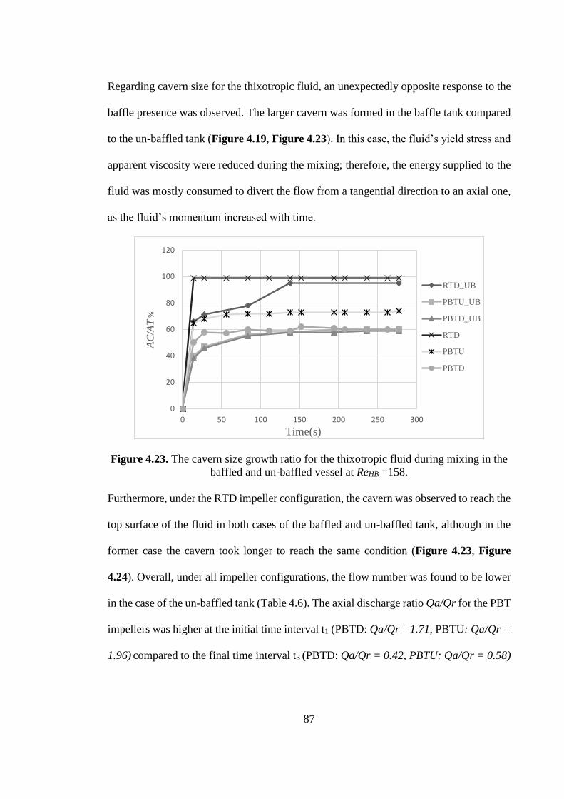
87
Regarding cavern size for the thixotropic fluid, an unexpectedly opposite response to the
baffle presence was observed. The larger cavern was formed in the baffle tank compared
to the un-baffled tank (Figure 4.19, Figure 4.23). In this case, the fluid’s yield stress and
apparent viscosity were reduced during the mixing; therefore, the energy supplied to the
fluid was mostly consumed to divert the flow from a tangential direction to an axial one,
as the fluid’s momentum increased with time.
Figure 4.23. The cavern size growth ratio for the thixotropic fluid during mixing in the
baffled and un-baffled vessel at ReHB =158.
Furthermore, under the RTD impeller configuration, the cavern was observed to reach the
top surface of the fluid in both cases of the baffled and un-baffled tank, although in the
former case the cavern took longer to reach the same condition (Figure 4.23, Figure
4.24). Overall, under all impeller configurations, the flow number was found to be lower
in the case of the un-baffled tank (Table 4.6). The axial discharge ratio Qa/Qr for the PBT
impellers was higher at the initial time interval t1 (PBTD: Qa/Qr =1.71, PBTU: Qa/Qr =
1.96) compared to the final time interval t3 (PBTD: Qa/Qr = 0.42, PBTU: Qa/Qr = 0.58)
0
20
40
60
80
100
120
0 50 100 150 200 250 300
AC
/AT
%
Time(s)
RTD_UB
PBTU_UB
PBTD_UB
RTD
PBTU
PBTD
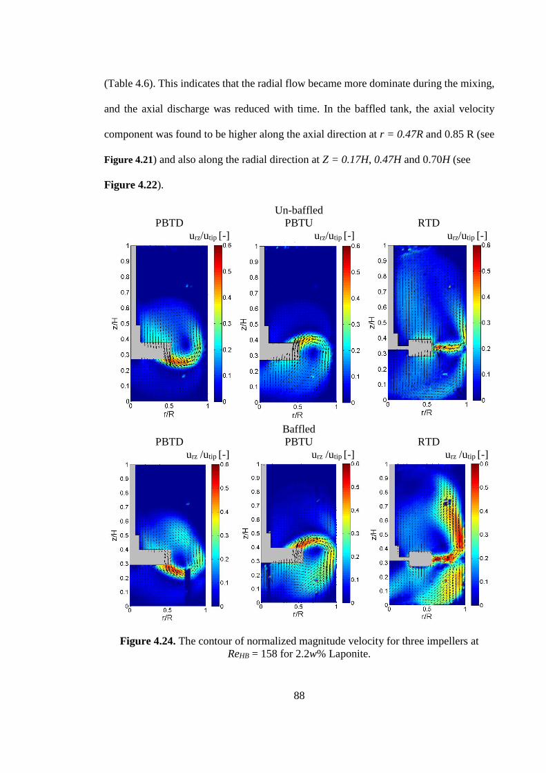
88
(Table 4.6). This indicates that the radial flow became more dominate during the mixing,
and the axial discharge was reduced with time. In the baffled tank, the axial velocity
component was found to be higher along the axial direction at r = 0.47R and 0.85 R (see
Figure 4.21) and also along the radial direction at Z = 0.17H, 0.47H and 0.70H (see
Figure 4.22).
Un-baffled
PBTD PBTU RTD
urz/utip [-]
urz/utip [-]
urz/utip [-]
Baffled
PBTD PBTU RTD
urz /utip [-]
urz /utip [-]
urz /utip [-]
Figure 4.24. The contour of normalized magnitude velocity for three impellers at
ReHB = 158 for 2.2w% Laponite.
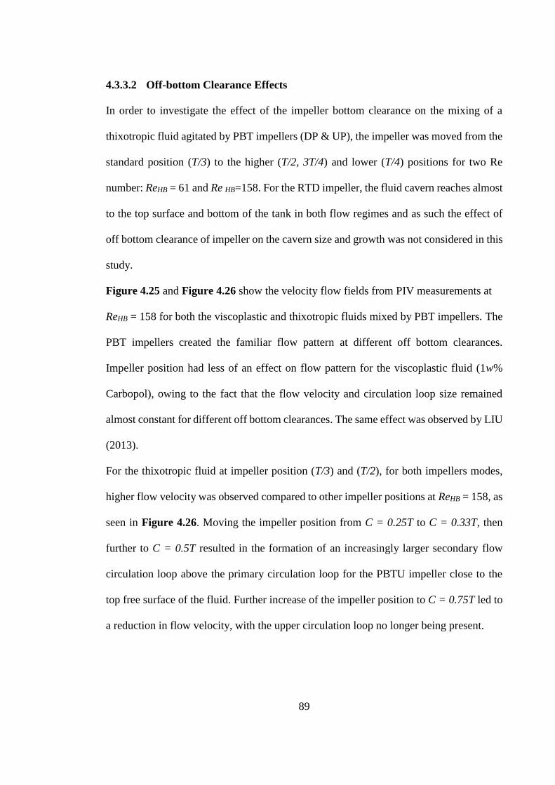
89
4.3.3.2 Off-bottom Clearance Effects
In order to investigate the effect of the impeller bottom clearance on the mixing of a
thixotropic fluid agitated by PBT impellers (DP & UP), the impeller was moved from the
standard position (T/3) to the higher (T/2, 3T/4) and lower (T/4) positions for two Re
number: ReHB = 61 and Re HB=158. For the RTD impeller, the fluid cavern reaches almost
to the top surface and bottom of the tank in both flow regimes and as such the effect of
off bottom clearance of impeller on the cavern size and growth was not considered in this
study.
Figure 4.25 and Figure 4.26 show the velocity flow fields from PIV measurements at
ReHB = 158 for both the viscoplastic and thixotropic fluids mixed by PBT impellers. The
PBT impellers created the familiar flow pattern at different off bottom clearances.
Impeller position had less of an effect on flow pattern for the viscoplastic fluid (1w%
Carbopol), owing to the fact that the flow velocity and circulation loop size remained
almost constant for different off bottom clearances. The same effect was observed by LIU
(2013).
For the thixotropic fluid at impeller position (T/3) and (T/2), for both impellers modes,
higher flow velocity was observed compared to other impeller positions at ReHB = 158, as
seen in Figure 4.26. Moving the impeller position from C = 0.25T to C = 0.33T, then
further to C = 0.5T resulted in the formation of an increasingly larger secondary flow
circulation loop above the primary circulation loop for the PBTU impeller close to the
top free surface of the fluid. Further increase of the impeller position to C = 0.75T led to
a reduction in flow velocity, with the upper circulation loop no longer being present.
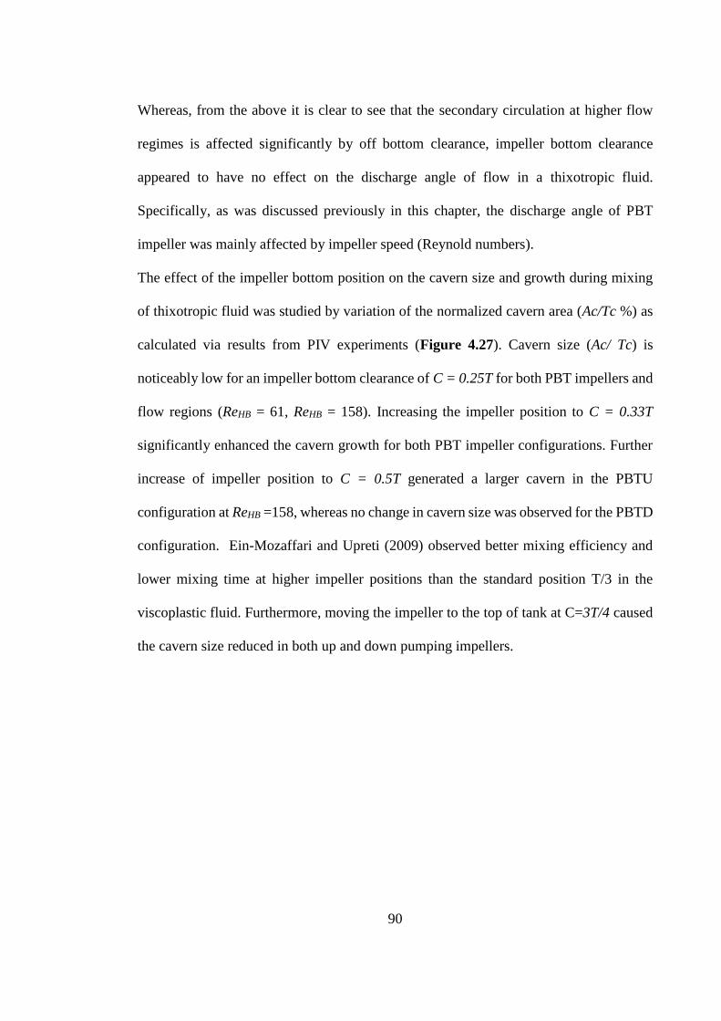
90
Whereas, from the above it is clear to see that the secondary circulation at higher flow
regimes is affected significantly by off bottom clearance, impeller bottom clearance
appeared to have no effect on the discharge angle of flow in a thixotropic fluid.
Specifically, as was discussed previously in this chapter, the discharge angle of PBT
impeller was mainly affected by impeller speed (Reynold numbers).
The effect of the impeller bottom position on the cavern size and growth during mixing
of thixotropic fluid was studied by variation of the normalized cavern area (Ac/Tc %) as
calculated via results from PIV experiments (Figure 4.27). Cavern size (Ac/ Tc) is
noticeably low for an impeller bottom clearance of C = 0.25T for both PBT impellers and
flow regions (ReHB = 61, ReHB = 158). Increasing the impeller position to C = 0.33T
significantly enhanced the cavern growth for both PBT impeller configurations. Further
increase of impeller position to C = 0.5T generated a larger cavern in the PBTU
configuration at ReHB =158, whereas no change in cavern size was observed for the PBTD
configuration. Ein-Mozaffari and Upreti (2009) observed better mixing efficiency and
lower mixing time at higher impeller positions than the standard position T/3 in the
viscoplastic fluid. Furthermore, moving the impeller to the top of tank at C=3T/4 caused
the cavern size reduced in both up and down pumping impellers.
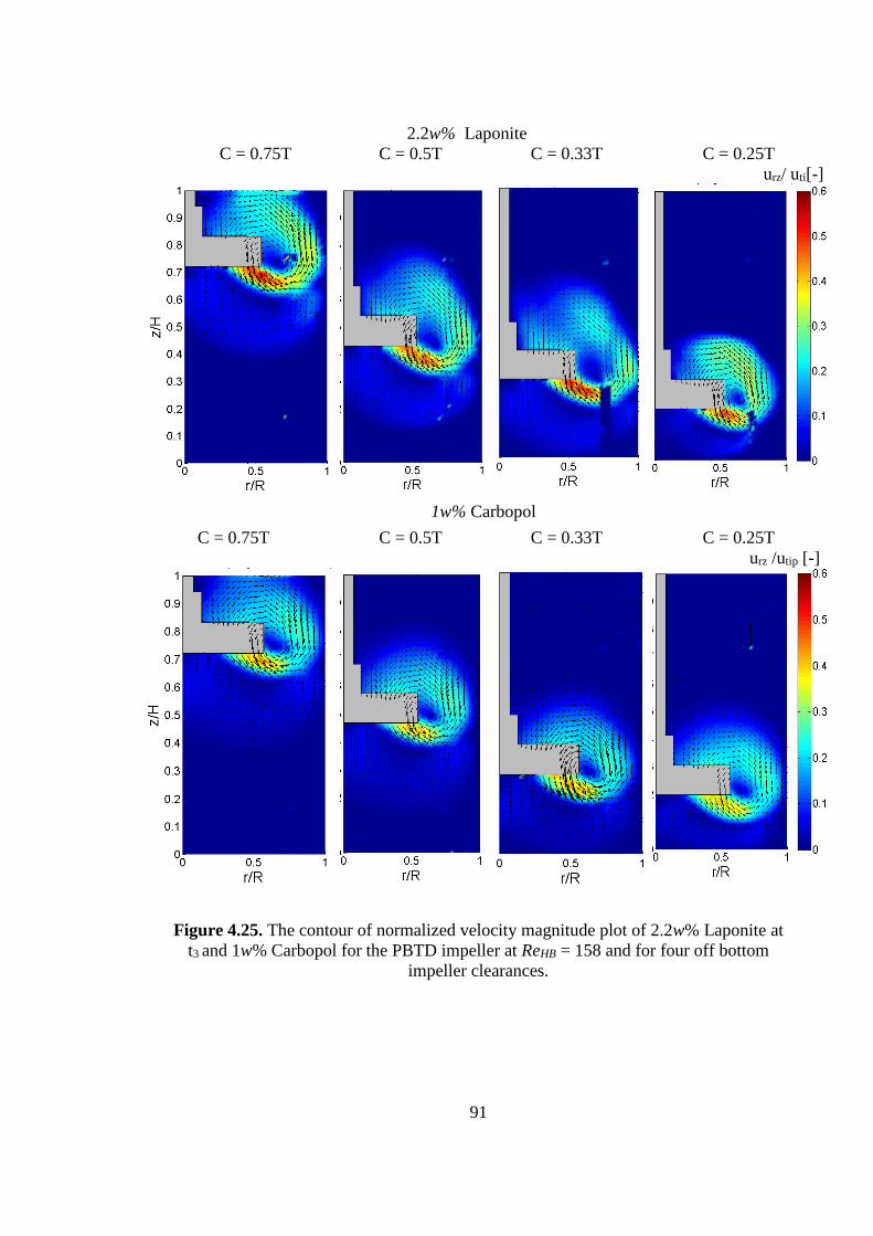
91
2.2w% Laponite
C = 0.75T C = 0.5T C = 0.33T C = 0.25T
urz/ uti[-]
1w% Carbopol
C = 0.75T C = 0.5T C = 0.33T C = 0.25T
urz /utip [-]
Figure 4.25. The contour of normalized velocity magnitude plot of 2.2w% Laponite at
t3 and 1w% Carbopol for the PBTD impeller at ReHB = 158 and for four off bottom
impeller clearances.
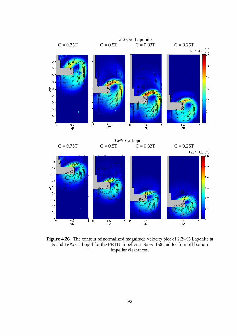
92
Figure 4.26. The contour of normalized magnitude velocity plot of 2.2w% Laponite at
t3 and 1w% Carbopol for the PBTU impeller at ReHB=158 and for four off bottom
impeller clearances.
2.2w% Laponite
C = 0.75T C = 0.5T C = 0.33T C = 0.25T
urz/ utip [-]
1w% Carbopol
C = 0.75T C = 0.5T C = 0.33T C = 0.25T
urz / utip [-]
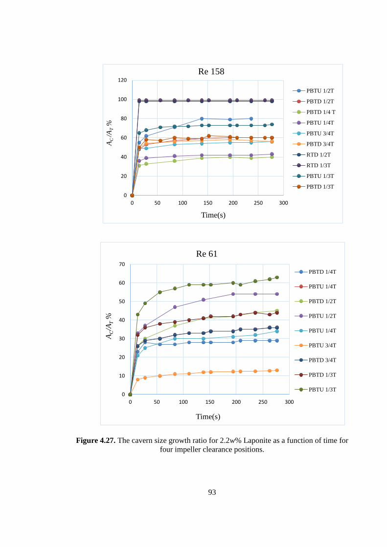
93
Figure 4.27. The cavern size growth ratio for 2.2w% Laponite as a function of time for
four impeller clearance positions.
0
20
40
60
80
100
120
0 50 100 150 200 250 300
AC
/AT
%
Time(s)
Re 158
PBTU 1/2T
PBTD 1/2T
PBTD 1/4 T
PBTU 1/4T
PBTU 3/4T
PBTD 3/4T
RTD 1/2T
RTD 1/3T
PBTU 1/3T
PBTD 1/3T
0
10
20
30
40
50
60
70
0 50 100 150 200 250 300
AC/A
T%
Time(s)
Re 61
PBTD 1/4T
PBTU 1/4T
PBTD 1/2T
PBTU 1/2T
PBTU 1/4T
PBTU 3/4T
PBTD 3/4T
PBTD 1/3T
PBTU 1/3T
94
4.4 Conclusions
In this chapter, a time-dependent thixotropic fluid (2.2w% Laponite) with yield stress
behavior was investigated within a stirred tank by means of two non-intrusive flow
visualization techniques, PIV and PLIF. To achieve this, a time-independent fluid (1w%
Carbopol) with a yield stress and shear-thinning properties was also analyzed as a
reference fluid, to help better observe the time effects on the thixotropic fluid mixing.
In this regard, flow pattern, normalized mean velocity and cavern growth in the tank was
characterized during the mixing for the thixotropic fluid, and the results were compared
to the reference fluid under three different flow regimes (ReHB = 7, ReHB = 61,
ReHB = 158).
The results suggest that under the PBT (UP & DP) impeller configuration, flow developed
with time and two flow patterns, as primary and secondary loops, were formed. The flow
reached a steady state condition at approximately t =138s for RHB =158. For the RTD
impeller, the flow fields of the thixotropic fluid showed an unexpectedly higher
magnitude velocity specifically in the vicinity of the impeller compared to the PBT
impellers and reached the steady state condition prematurely. The above can be seen in
the following:
a) The shear strain plot Figure 4.11 shows that the shear applied to the fluid in the vicinity
of the impeller was found to be much higher in the RTD impeller compared to the PBT
impellers.
b) A high shear was applied by RTD impeller mostly in a radial direction, causing the
viscosity of the fluid to reduce more quickly.
95
Lowering the Reynold number to ReHB = 7 saw a further significant reduction in
magnitude velocity and pumping capacity under the three impeller configurations, with
the flow pattern of the radial RTD impeller changing most noticeably. In this case, the
flow was observed to leave the impeller blades at an angle to the radial direction in spite
of a fully radially discharged impeller being used.
While both fluids showed the presence of cavern in mixing, due to yield stress, reduction
of apparent viscosity with time helped the cavern to develop in the case of the thixotropic
fluid. Therefore, the cavern sizes in Figure 4.16 and Figure 4.19 are larger for 2.2w%
Laponite relative to 1w%Carbopl. Under the RTD impeller configuration and at
ReHB = 158, the cavern for the thixotropic fluid reached to the top surface of the tank. A
PBTU impeller developed a bigger cavern at ReHB =158 and ReHB = 61 compared to the
PBTD impeller. Furthermore, it was found that impeller design did not contribute to
cavern evolution at a low Reynold number regime as the trend and size of the caverns
under the three impeller configurations remained almost the same for the thixotropic fluid.
In addition the thixotropic fluids in an un-baffled vessel configuration, show noticeably
different behavior when compared to a viscoplastic fluid. In the case of the baffled vessel,
the cavern size become larger, and improved flow fields are obtained compared to an un-
baffled case. In viscoplastic fluids, however, the conventional baffled vessel reduces the
mixing efficiency by reducing cavern size and flow velocity.
The yield stress and apparent viscosity of the studied thixotropic fluid declined with time
during stirring, meaning the energy supplied to the fluid is mostly consumed to divert the
flow from a tangential direction to an axial one. In viscoplastic fluids a yield stress acts
as a barrier to the fluid momentum.
96
Increasing the impeller bottom clearance from C = 0.25T to a higher position of C =
0.33T significantly enhanced the cavern size and flow field for all impeller configurations.
With further increase of clearance to C = 0.5T, the cavern size becomes larger for the
PBTU impeller, whereas no significant effect was found in the other impeller
configurations. Moving the impeller to a higher position of C = 0.75T resulted in the
inverse effect on cavern growth and flow field for all the three impeller types.
Overall, compared to the reference fluid, the thixotropic fluid with yield stress generates
improved flow fields and larger cavern size and demand less energy during mixing.
97
5 Chapter 5
THE EFFECT OF VISCOELASTICITY IN A STIRRED TANK
This chapter aims to study the effects of elasticity and shear-thinning behavior of fluids
on their flow and mixing by using model fluids that exhibit only one of these behaviors
at a time. Thus, the effects of each rheological behavior can be separately studied and
identified. Viscoelastic Boger fluids with constant viscosity were used to investigate the
elasticity effect on mixing. An inelastic shear-thinning fluid assisited in the understanding
of the shear-thinning effect on mixing in the absence of elasticity. In addition the
behaviour of viscous Newtonian fluids was studied whilst using them as reference fluids.
Particle Image Velocimetry (PIV) was applied to visualize the flow behavior of the
viscoelastic, the shear-thinning and the Newtonian fluids. Flow pattern and velocity were
investigated in the stirred tank using three impeller configurations: Pitch Blade Turbine
in both up and down pumping mode (PBTD, PBTU) and Ruston Disk Turbine (RTD).
5.1 Introduction
Mixing of viscoelastic fluids is common to many chemical and biochemical process
industries and yet there is very little known about the effects of fluid elasticity on mixing
performance. Elasticity impacts mixing in two ways: it can affect the power required for
agitation and it can change flow patterns, as such it can influence the time needed for
homogenization (Collias and Prud'homme, 1985).
98
Most viscoelastic fluids show a combination of rheologically complex behaviors and
therefore it is difficult to separate the effect of viscoelasticity from these other behaviors.
In 1977, Boger introduced a liquid that exhibited a constant high viscosity but was elastic
at room temperature. Therefore, by using this liquid the effect of elasticity can be studied
in the absence of shear-thinning effects. Another property of this fluid is that it is optically
clear, which is important to flow visualization measurements (Mackay and Boger, 1987).
The first Boger fluid was introduced as a solution of polyacrylamide in a concentrated
sugar solution (corn syrup) and had high elasticity with a constant, high viscosity close
to 22 Pa·s, (Boger and Nguyen, 1978). Later Prilutski et al. (1983) introduced a new
formulation of the Boger fluid which was a mixture of polyisobutylene (PIB) in
Polybutene (PB) and a small amount of kerosene oil. The disadvantage of using this fluid
is that the PB solutions requires large amounts of an organic solvent for cleaning, making
it hard to work with and expensive. More detail of rheological characteristics of other
formulations of the Boger fluid can be found in a recent review of James (2009). The
difficulties encountered using the first Boger fluid (polyacrylamide-corn syrup mix) in a
rheometer were reported by Choplin and Carreau (1986) and the two major ones are as
follow: i) formation of corn syrup crystals when exposed to air ii) rheological properties
are not reproducible from one batch to another. Choplin and Carreau (1986) therefore
proposed a new solution of polyacrylamide in a mixture of glycerin and water, which
exhibited lower viscosity and elasticity. This formulation was also used in the work
presented in this thesis.
There are a few select studies investigating hydrodynamics of viscoelastic fluids, with
most of the research being focused on studying mixing effects such as mixing times or
99
power draw. However, mixing effects may vary from on study to another and are
dependent on the flow regimes and the type of viscoelastic fluids used (e.g. shear-thinning
and elastic fluids will give different results to Boger fluids). Elastic forces in viscoelastic
fluids are opposed to the centrifugal forces, reducing the formation of a vortex and often
causing the viscoelastic fluid to climb a rotating shaft (Collias and Prud'homme, 1985).
The effect of elasticity on power consumption is studied by measuring the torque on the
mixing vessel. Özcan-Taskin and Nienow (1995) investigated the power consumption in
the mixing of Boger fluids. A much more recent work conducted by Seyssiecq and
Tolofoudy (2003) used a Boger fluid to monitor power consumption in a stirred tank. It
was observed that in the laminar region the power consumption of the specific Boger fluid
showed a 300% increase compared to that of a Newtonian fluid, whereas in the low
transitional region a 15% increase in power consumption was observed for the Boger fluid
with respect to the Newtonian fluid (Seyssiecq and Tolofoudy, 2003).
The study of flow patterns is of upmost importance, as flow patterns show how the system
is mixed. The formation, shape and velocities of these flow patterns are critical to
designing and optimization of mixing systems. Nonetheless, little research has been
performed in this area. Stokes (1998) examined the confined swirling flow of Boger fluids
with different viscosities for situations where inertia or elasticity dominated the flow
field. The Elasticity number, El, which characterizes the elasticity of fluids, is the
parameter that defines the flow field (Stokes, 1998, Stokes et al., 2001).
The present work is focused on the effects of viscoelasticity and shear-thinning on mixing
in a stirred vessel with three type of impellers (PBTD, PBTU, RTD), as observed by using
the powerful, non-intrusive, flow visualization technique of PIV. Flow dynamics of
100
viscoelastic fluid and shear-thinning fluid have been determined from PIV measurements
and compared to respective results for the Newtonian fluid.
5.2 Rheology and Material Characterization
5.2.1 Test fluids
Five fluids were used in this study: two viscous Newtonian fluids (N93, N95), two
viscoelastic Boger fluids (100PAA and 300PAA), and a shear-thinning inelastic fluid
(1.5w% CMC). The complete composition of the fluids used can be found in Table 5.1.
5.2.1.1 Viscoelastic Fluid (Boger Fluid)
The Boger fluids exhibited a constant viscosity but were elastic at room temperature. In
addition, their optical transparency was imperative in obtaining results from the PIV flow
visualization technique (Mackay and Boger, 1987). The Boger fluids (100PAA,
300PAA) used in this work were prepared by first dissolving a small amount of
polyacrylamide (PAA) Separan AP30 (supplied by SNF Ltd, UK) into deionized water
to make a stock solution. According to the manufacturer’s specifications, AP30 has a
molecular weight (Mw) of approximately 5×10⁶. The water was heated to about 30-
40°C, and the polymer was added little by little to the water that was being constantly
mixed by a magnetic stirrer in order to facilitate the dispersion of the polymer and to
avoid agglomeration. To reduce bacteriological degradation of the solution biocide
Kathon LXE, (produced by Rohm and Haas, UK) was added to the fluid. NaCl was also
added to the stock solution to reduce the shear-thinning effect in the Boger fluids. Details
on the effects of salt concentration on the rheology of viscoelastic fluids can be seen in
Stokes (1998). The stock solution was placed on an overhead stirrer at very a low rotation
rate of 80 rpm, until the polymer was completely dissolved. The experimental solutions
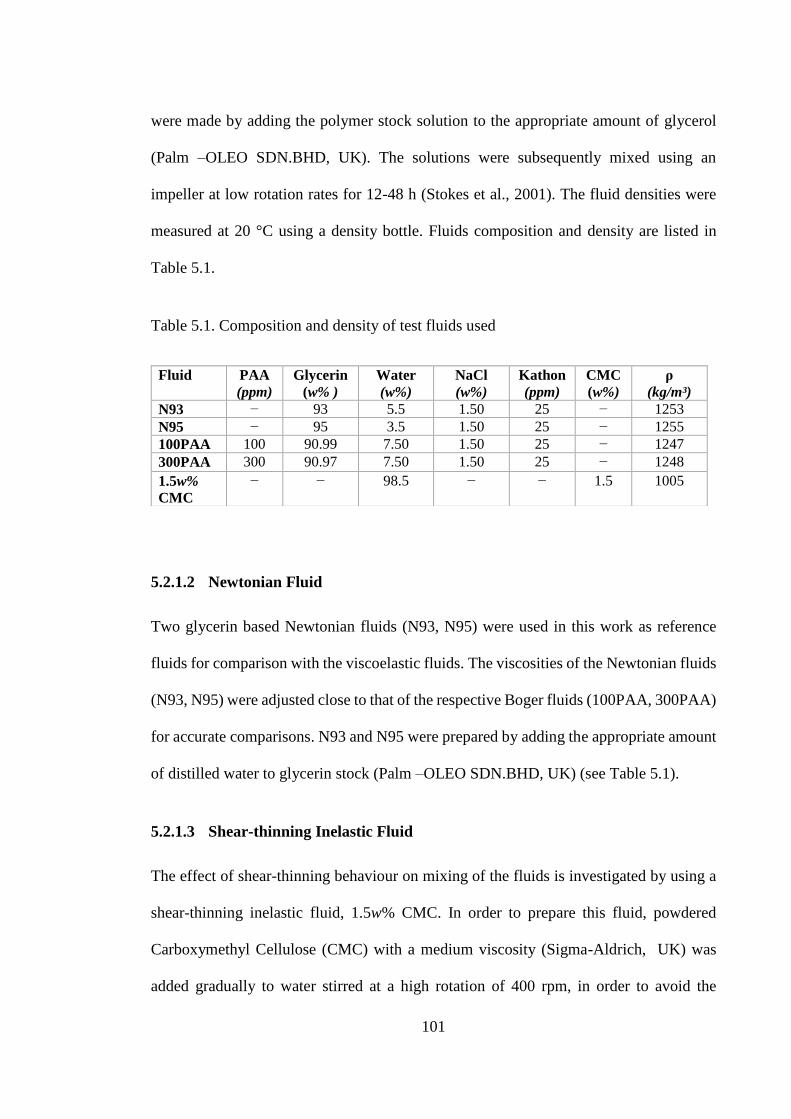
101
were made by adding the polymer stock solution to the appropriate amount of glycerol
(Palm –OLEO SDN.BHD, UK). The solutions were subsequently mixed using an
impeller at low rotation rates for 12-48 h (Stokes et al., 2001). The fluid densities were
measured at 20 °C using a density bottle. Fluids composition and density are listed in
Table 5.1.
Table 5.1. Composition and density of test fluids used
5.2.1.2 Newtonian Fluid
Two glycerin based Newtonian fluids (N93, N95) were used in this work as reference
fluids for comparison with the viscoelastic fluids. The viscosities of the Newtonian fluids
(N93, N95) were adjusted close to that of the respective Boger fluids (100PAA, 300PAA)
for accurate comparisons. N93 and N95 were prepared by adding the appropriate amount
of distilled water to glycerin stock (Palm –OLEO SDN.BHD, UK) (see Table 5.1).
5.2.1.3 Shear-thinning Inelastic Fluid
The effect of shear-thinning behaviour on mixing of the fluids is investigated by using a
shear-thinning inelastic fluid, 1.5w% CMC. In order to prepare this fluid, powdered
Carboxymethyl Cellulose (CMC) with a medium viscosity (Sigma-Aldrich, UK) was
added gradually to water stirred at a high rotation of 400 rpm, in order to avoid the
Fluid PAA
(ppm)
Glycerin
(w% )
Water
(w%)
NaCl
(w%)
Kathon
(ppm)
CMC
(w%)
ρ
(kg/m³)
N93 − 93 5.5 1.50 25 − 1253
N95 − 95 3.5 1.50 25 − 1255
100PAA 100 90.99 7.50 1.50 25 − 1247
300PAA 300 90.97 7.50 1.50 25 − 1248
1.5w%
CMC
− − 98.5 − − 1.5 1005
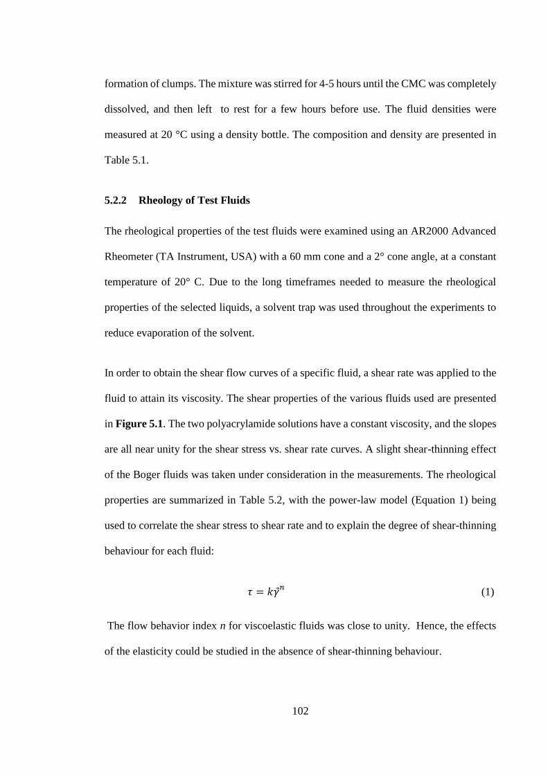
102
formation of clumps. The mixture was stirred for 4-5 hours until the CMC was completely
dissolved, and then left to rest for a few hours before use. The fluid densities were
measured at 20 °C using a density bottle. The composition and density are presented in
Table 5.1.
5.2.2 Rheology of Test Fluids
The rheological properties of the test fluids were examined using an AR2000 Advanced
Rheometer (TA Instrument, USA) with a 60 mm cone and a 2° cone angle, at a constant
temperature of 20° C. Due to the long timeframes needed to measure the rheological
properties of the selected liquids, a solvent trap was used throughout the experiments to
reduce evaporation of the solvent.
In order to obtain the shear flow curves of a specific fluid, a shear rate was applied to the
fluid to attain its viscosity. The shear properties of the various fluids used are presented
in Figure 5.1. The two polyacrylamide solutions have a constant viscosity, and the slopes
are all near unity for the shear stress vs. shear rate curves. A slight shear-thinning effect
of the Boger fluids was taken under consideration in the measurements. The rheological
properties are summarized in Table 5.2, with the power-law model (Equation 1) being
used to correlate the shear stress to shear rate and to explain the degree of shear-thinning
behaviour for each fluid:
𝜏 = 𝑘𝛾 𝑛 (1)
The flow behavior index n for viscoelastic fluids was close to unity. Hence, the effects
of the elasticity could be studied in the absence of shear-thinning behaviour.
103
Consequently, the power low model was fitted to the experimental measurements from
the shear-thinning fluid 1.5w% CMC, which resulted in the values of k = 0.49 and n =
0.77, whereas the apparent viscosity of the fluid remained similar to that of the other
fluids, as listed in Table 5.2. The viscosities for the two Newtonian fluids N93 and N95
were found to be similar to those of 100PAA and 300PAA respectively, as shown in
Figure 5.1.
The primary normal stress difference (N1) against the shear rate for the two Boger fluids
that have different degrees of elasticity is presented in Figure 5.2. In addtion the first
normal stress difference (N1) was correlated to the shear rate using the power law (Özcan-
Taskin, 1993):
𝑁1 = 𝐴𝛾 𝑏 (2)
where A and b are arbitrary constants. The value of A and b are shown in Table 5.2 for
the two Boger fluids. The second normal stress difference (N2) is generally much smaller
than N1 and is difficult to measure with normal a rheometer, subsequently being usually
neglected in measurements. More details of the measurement for the second normal stress
difference for a highly elastic Boger fluid can be found in the work of Magda et al. (1991).
104
Figure 5.1. Steady shear properties for all tests fluids a), viscosity versus shear rate
and b) shear stress versus shear rate.
(a)
Shear rate (s-1
)
0.1 1 10 100 1000
visc
osi
ty (
Pa
.s)
0.1
1
1.5w% CMC
100 PAA
300 PAA
N93
N95
(b)
Shear rate (s-1
)
1 10 100 1000
She
ar
stre
ss (
Pa
)
0.1
1
10
100
1000
1.5w% CMC
100 PAA
300 PAA
N93
N95
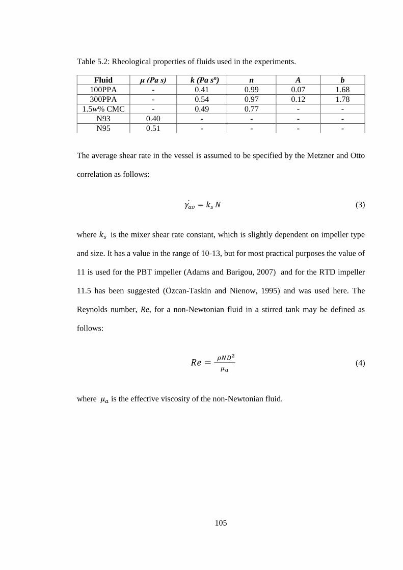
105
Table 5.2: Rheological properties of fluids used in the experiments.
The average shear rate in the vessel is assumed to be specified by the Metzner and Otto
correlation as follows:
𝛾𝑎𝑣 = 𝑘𝑠 𝑁 (3)
where 𝑘𝑠 is the mixer shear rate constant, which is slightly dependent on impeller type
and size. It has a value in the range of 10-13, but for most practical purposes the value of
11 is used for the PBT impeller (Adams and Barigou, 2007) and for the RTD impeller
11.5 has been suggested (Özcan-Taskin and Nienow, 1995) and was used here. The
Reynolds number, Re, for a non-Newtonian fluid in a stirred tank may be defined as
follows:
𝑅𝑒 = 𝜌𝑁𝐷2
𝜇𝑎 (4)
where 𝜇𝑎 is the effective viscosity of the non-Newtonian fluid.
Fluid μ (Pa s) k (Pa sn) n A b
100PPA - 0.41 0.99 0.07 1.68
300PPA - 0.54 0.97 0.12 1.78
1.5w% CMC - 0.49 0.77 - -
N93 0.40 - - - -
N95 0.51 - - - -
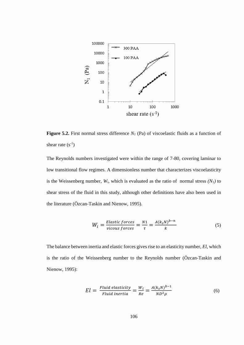
106
Figure 5.2. First normal stress difference N1 (Pa) of viscoelastic fluids as a function of
shear rate (s-1)
The Reynolds numbers investigated were within the range of 7-80, covering laminar to
low transitional flow regimes. A dimensionless number that characterizes viscoelasticity
is the Weissenberg number, Wi, which is evaluated as the ratio of normal stress (N1) to
shear stress of the fluid in this study, although other definitions have also been used in
the literature (Özcan-Taskin and Nienow, 1995).
𝑊𝑖 =𝐸𝑙𝑎𝑠𝑡𝑖𝑐 𝑓𝑜𝑟𝑐𝑒𝑠
𝑣𝑖𝑐𝑜𝑢𝑠 𝑓𝑜𝑟𝑐𝑒𝑠=
𝑁1
𝜏=
𝐴(𝑘𝑠𝑁)𝑏−𝑛
𝑘 (5)
The balance between inertia and elastic forces gives rise to an elasticity number, El, which
is the ratio of the Weissenberg number to the Reynolds number (Özcan-Taskin and
Nienow, 1995):
𝐸𝑙 = 𝐹𝑙𝑢𝑖𝑑 𝑒𝑙𝑎𝑠𝑡𝑖𝑐𝑖𝑡𝑦
𝐹𝑙𝑢𝑖𝑑 𝑖𝑛𝑒𝑟𝑡𝑖𝑎=
𝑊𝑖
𝑅𝑒=
𝐴(𝑘𝑠𝑁)𝑏−1
𝑁𝐷2𝜌 (6)
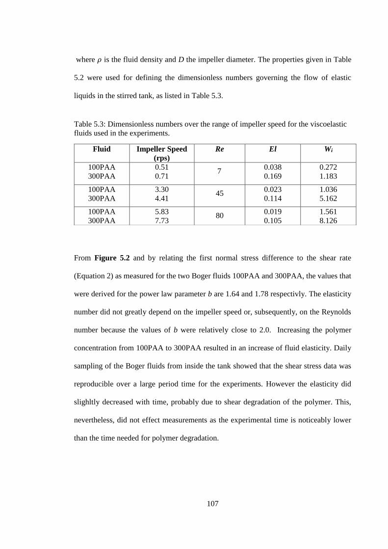
107
where 𝜌 is the fluid density and D the impeller diameter. The properties given in Table
5.2 were used for defining the dimensionless numbers governing the flow of elastic
liquids in the stirred tank, as listed in Table 5.3.
Table 5.3: Dimensionless numbers over the range of impeller speed for the viscoelastic
fluids used in the experiments.
From Figure 5.2 and by relating the first normal stress difference to the shear rate
(Equation 2) as measured for the two Boger fluids 100PAA and 300PAA, the values that
were derived for the power law parameter b are 1.64 and 1.78 respectivly. The elasticity
number did not greatly depend on the impeller speed or, subsequently, on the Reynolds
number because the values of b were relatively close to 2.0. Increasing the polymer
concentration from 100PAA to 300PAA resulted in an increase of fluid elasticity. Daily
sampling of the Boger fluids from inside the tank showed that the shear stress data was
reproducible over a large period time for the experiments. However the elasticity did
slighltly decreased with time, probably due to shear degradation of the polymer. This,
nevertheless, did not effect measurements as the experimental time is noticeably lower
than the time needed for polymer degradation.
Fluid
Impeller Speed
(rps)
Re El Wi
100PAA
300PAA
0.51
0.71 7
0.038
0.169
0.272
1.183
100PAA
300PAA
3.30
4.41 45
0.023
0.114
1.036
5.162
100PAA
300PAA
5.83
7.73 80
0.019
0.105
1.561
8.126
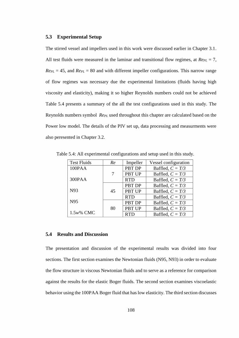
108
5.3 Experimental Setup
The stirred vessel and impellers used in this work were discussed earlier in Chapter 3.1.
All test fluids were measured in the laminar and transitional flow regimes, at RePL = 7,
RePL = 45, and RePL = 80 and with different impeller configurations. This narrow range
of flow regimes was necessary due the experimental limitations (fluids having high
viscosity and elasticity), making it so higher Reynolds numbers could not be achieved
Table 5.4 presents a summary of the all the test configurations used in this study. The
Reynolds numbers symbol RePL used throughout this chapter are calculated based on the
Power low model. The details of the PIV set up, data processing and measurments were
also peresented in Chapter 3.2.
Table 5.4: All experimental configurations and setup used in this study.
5.4 Results and Discussion
The presentation and discussion of the experimental results was divided into four
sections. The first section examines the Newtonian fluids (N95, N93) in order to evaluate
the flow structure in viscous Newtonian fluids and to serve as a reference for comparison
against the results for the elastic Boger fluids. The second section examines viscoelastic
behavior using the 100PAA Boger fluid that has low elasticity. The third section discusses
Test Fluids Re Impeller Vessel configuration
100PAA
300PAA
N93
N95
1.5w% CMC
7
PBT DP Baffled, C = T/3
PBT UP Baffled, C = T/3
RTD Baffled, C = T/3
45
PBT DP Baffled, C = T/3
PBT UP Baffled, C = T/3
RTD Baffled, C = T/3
80
PBT DP Baffled, C = T/3
PBT UP Baffled, C = T/3
RTD Baffled, C = T/3
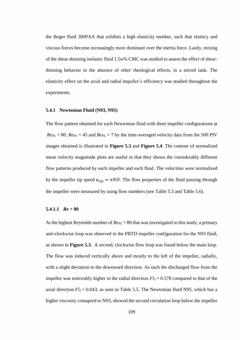
109
the Boger fluid 300PAA that exhibits a high elasticity number, such that elasticy and
viscous forces become increasingly more dominant over the inertia force. Lastly, mixing
of the shear-thinning inelastic fluid 1.5w% CMC was studied to assess the effect of shear-
thinning behavior in the absence of other rheological effects, in a stirred tank. The
elasticity effect on the axial and radial impeller’s efficiency was studied throughout the
experiments.
5.4.1 Newtonian Fluid (N93, N95)
The flow pattern obtained for each Newtonian fluid with three impeller configurations at
RePL = 80, RePL = 45 and RePL = 7 by the time-averaged velocity data from the 500 PIV
images obtained is illustrated in Figure 5.3 and Figure 5.4. The contour of normalized
mean velocity magnitude plots are useful in that they shows the considerably different
flow patterns produced by each impeller and each fluid. The velocities were normalized
by the impeller tip speed 𝑢𝑡𝑖𝑝 = 𝜋𝑁𝐷. The flow properties of the fluid passing through
the impeller were measured by using flow numbers (see Table 5.5 and Table 5.6).
5.4.1.1 Re = 80
At the highest Reynolds number of RePL = 80 that was investigated in this study, a primary
anti-clockwise loop was observed in the PBTD impeller configuration for the N93 fluid,
as shown in Figure 5.3. A second, clockwise flow loop was found below the main loop.
The flow was induced vertically above and mostly to the left of the impeller, radially,
with a slight deviation to the downward direction. As such the discharged flow from the
impeller was noticeably higher in the radial direction Fl3 = 0.578 compared to that of the
axial direction Fl2 = 0.043, as seen in Table 5.5. The Newtonian fluid N95, which has a
higher viscosity comapred to N93, showed the second circulation loop below the impeller
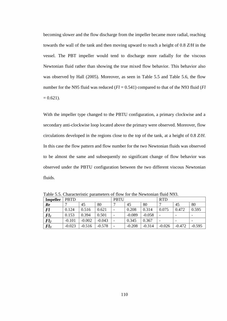
110
becoming slower and the flow discharge from the impeller became more radial, reaching
towards the wall of the tank and then moving upward to reach a height of 0.8 Z/H in the
vessel. The PBT impeller would tend to discharge more radially for the viscous
Newtonian fluid rather than showing the true mixed flow behavior. This behavior also
was observed by Hall (2005). Moreover, as seen in Table 5.5 and Table 5.6, the flow
number for the N95 fluid was reduced (Fl = 0.541) compared to that of the N93 fluid (Fl
= 0.621).
With the impeller type changed to the PBTU configuration, a primary clockwise and a
secondary anti-clockwise loop located above the primary were observed. Moreover, flow
circulations developed in the regions close to the top of the tank, at a height of 0.8 Z/H.
In this case the flow pattern and flow number for the two Newtonian fluids was observed
to be almost the same and subsequently no significant change of flow behavior was
observed under the PBTU configuration between the two different viscous Newtonian
fluids.
Table 5.5. Characteristic parameters of flow for the Newtonian fluid N93.
Impeller PBTD PBTU RTD
Re 7 45 80 7 45 80 7 45 80
Fl 0.124 0.516 0.621 - 0.208 0.314 0.075 0.472 0.595
Fl1 0.153 0.394 0.501 - -0.089 -0.058 - - -
Fl2 -0.101 -0.002 -0.043 - 0.345 0.367 - - -
Fl3 -0.023 -0.516 -0.578 - -0.208 -0.314 -0.026 -0.472 -0.595
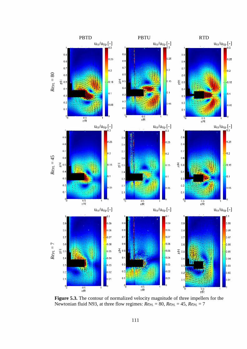
111
PBTD PBTU RTD
Re P
L =
80
urz/utip [-]
urz/utip [-]
urz/utip [-]
Re P
L =
45
urz/utip [-]
urz/utip [-]
urz/utip [-]
Re P
L =
7
urz/utip [-]
urz/utip [-]
urz/utip [-]
Figure 5.3. The contour of normalized velocity magnitude of three impellers for the
Newtonian fluid N93, at three flow regimes: RePL = 80, RePL = 45, RePL = 7
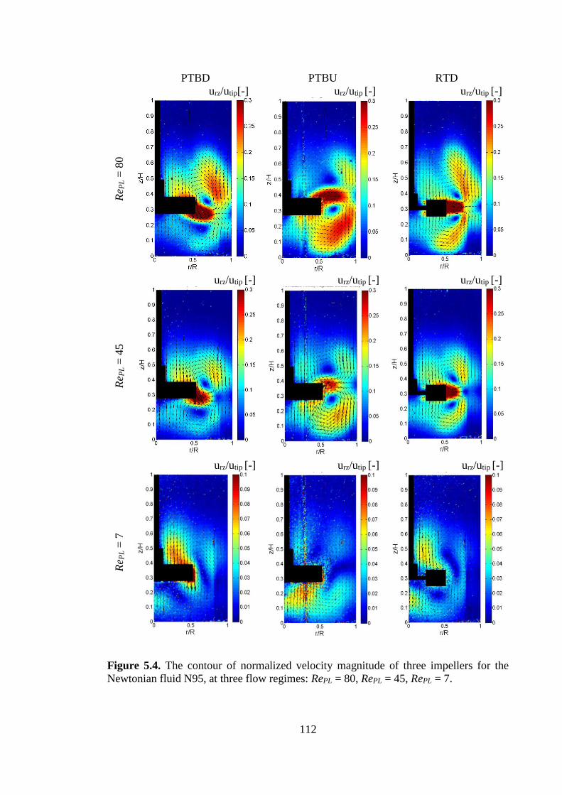
112
Figure 5.4. The contour of normalized velocity magnitude of three impellers for the
Newtonian fluid N95, at three flow regimes: RePL = 80, RePL = 45, RePL = 7.
PTBD PTBU RTD
Re P
L =
80
urz/utip[-]
urz/utip [-]
urz/utip [-]
Re P
L =
45
urz/utip [-]
urz/utip [-]
urz/utip [-]
Re P
L =
7
urz/utip [-]
urz/utip [-]
urz/utip [-]
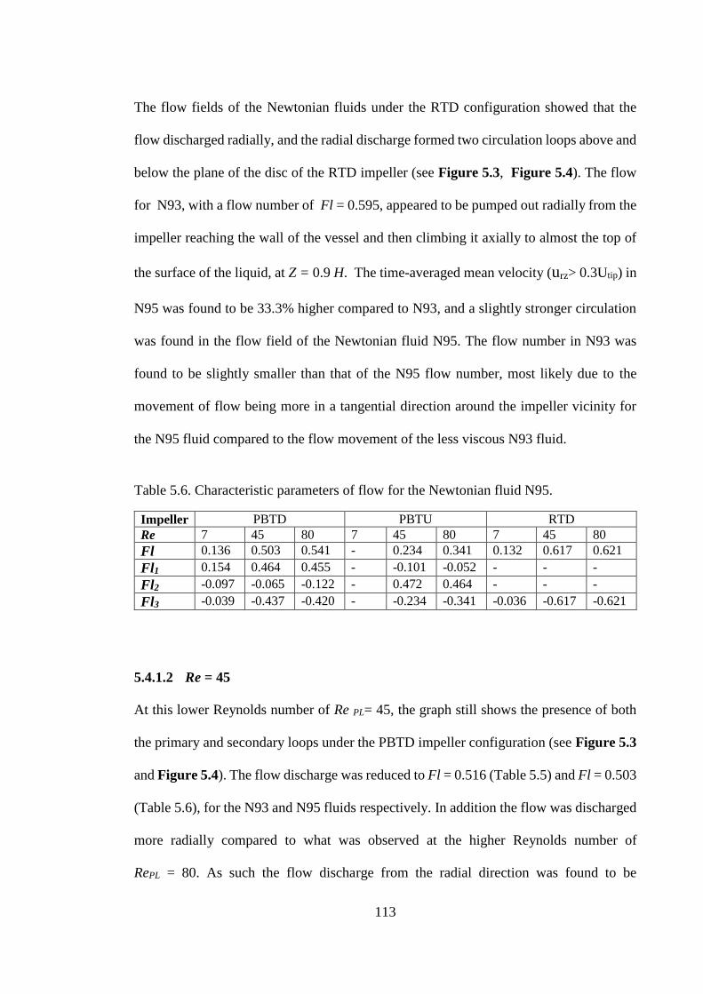
113
The flow fields of the Newtonian fluids under the RTD configuration showed that the
flow discharged radially, and the radial discharge formed two circulation loops above and
below the plane of the disc of the RTD impeller (see Figure 5.3, Figure 5.4). The flow
for N93, with a flow number of Fl = 0.595, appeared to be pumped out radially from the
impeller reaching the wall of the vessel and then climbing it axially to almost the top of
the surface of the liquid, at Z = 0.9 H. The time-averaged mean velocity (urz> 0.3Utip) in
N95 was found to be 33.3% higher compared to N93, and a slightly stronger circulation
was found in the flow field of the Newtonian fluid N95. The flow number in N93 was
found to be slightly smaller than that of the N95 flow number, most likely due to the
movement of flow being more in a tangential direction around the impeller vicinity for
the N95 fluid compared to the flow movement of the less viscous N93 fluid.
Table 5.6. Characteristic parameters of flow for the Newtonian fluid N95.
5.4.1.2 Re = 45
At this lower Reynolds number of Re PL= 45, the graph still shows the presence of both
the primary and secondary loops under the PBTD impeller configuration (see Figure 5.3
and Figure 5.4). The flow discharge was reduced to Fl = 0.516 (Table 5.5) and Fl = 0.503
(Table 5.6), for the N93 and N95 fluids respectively. In addition the flow was discharged
more radially compared to what was observed at the higher Reynolds number of
RePL = 80. As such the flow discharge from the radial direction was found to be
Impeller PBTD PBTU RTD
Re 7 45 80 7 45 80 7 45 80
Fl 0.136 0.503 0.541 - 0.234 0.341 0.132 0.617 0.621
Fl1 0.154 0.464 0.455 - -0.101 -0.052 - - -
Fl2 -0.097 -0.065 -0.122 - 0.472 0.464 - - -
Fl3 -0.039 -0.437 -0.420 - -0.234 -0.341 -0.036 -0.617 -0.621
114
significantly higher Fl3 = 0.516 and Fl3 = 0.437 for N93 and N95 respectively - compared
to the flow discharge from the axial direction, Fl2 (see Table 5.5 and Table 5.6). Under
the PBTU configuration the pumping capacity Fl was reduced (Fl = 0.208 and Fl = 0.231
for N93 and N95 respectively) compared to that seen at the higher Reynolds number (see
Table 5.5, Table 5.6). This reduction trend in pumping capacity of the impeller with
decreasing Reynolds number was also observed by (Rice et al., 2006).
5.4.1.3 Re = 7
At the lowest studied Reynolds number, RePL = 7, under the PBTD configuration the fluid
flow showed a reduction in terms of velocity and circulation. The flow was induced
vertically to the impeller and left it in mostly an axial direction, hence the Fl2 is
significantly higher compared to the Fl3 for both Newtonian fluids (see Table 5.5, Table
5.6). From Table 5.5 and Table 5.6 it is obvious that the flow pumping capacity was also
reduced significantly (Fl = 0.124 and Fl = 0.136 for N93 and N95 respectively) for both
Newtonian fluids under the PBTD configuration. For the RTD impeller the flow number
was measured (Fl = 0.075 and Fl = 0.132 for N93 and N95 respectively) and found to be
slightly lower than that reported by Rice et al. (2006), who measured Fl = 0.21. This
difference is due to the fact that a fluid with higher viscosity was used in the present work.
The flow pattern also changed significantly under a radial RTD impeller. In this case, the
flow that was induced from the impeller blades was at an angle to the radial direction and
formed two circulation loops in the tank. This diverse flow pattern made by the RTD
impeller was observed for Newtonian and shear-thinning fluids by both Rice et al. (2006)
and Arratia et al. (2006).
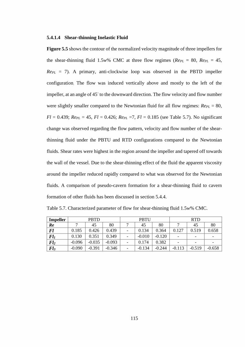
115
5.4.1.4 Shear-thinning Inelastic Fluid
Figure 5.5 shows the contour of the normalized velocity magnitude of three impellers for
the shear-thinning fluid 1.5w% CMC at three flow regimes (RePL = 80, RePL = 45,
RePL = 7). A primary, anti-clockwise loop was observed in the PBTD impeller
configuration. The flow was induced vertically above and mostly to the left of the
impeller, at an angle of 45◦ to the downward direction. The flow velocity and flow number
were slightly smaller compared to the Newtonian fluid for all flow regimes: RePL = 80,
Fl = 0.439; RePL = 45, Fl = 0.426; RePL =7, Fl = 0.185 (see Table 5.7). No significant
change was observed regarding the flow pattern, velocity and flow number of the shear-
thinning fluid under the PBTU and RTD configurations compared to the Newtonian
fluids. Shear rates were highest in the region around the impeller and tapered off towards
the wall of the vessel. Due to the shear-thinning effect of the fluid the apparent viscosity
around the impeller reduced rapidly compared to what was observed for the Newtonian
fluids. A comparison of pseudo-cavern formation for a shear-thinning fluid to cavern
formation of other fluids has been discussed in section 5.4.4.
Table 5.7. Characterized parameter of flow for shear-thinning fluid 1.5w% CMC.
Impeller PBTD PBTU RTD
Re 7 45 80 7 45 80 7 45 80
Fl 0.185 0.426 0.439 - 0.134 0.364 0.127 0.519 0.658
Fl1 0.130 0.351 0.349 - -0.010 -0.120 - - -
Fl2 -0.096 -0.035 -0.093 - 0.174 0.382 - - -
Fl3 -0.090 -0.391 -0.346 - -0.134 -0.244 -0.113 -0.519 -0.658
116
5.4.2 Low viscoelastic Boger Fluids (100PAA)
The flow patterns of a viscoelastic fluid depend highly on the viscoelasticity of the fluid
(Wi) (elasticity force/viscous force) and the range of operation (Re) (inertial force/viscous
force). The contour of normalized velocity magnitude and streamline of the Boger fluid
100PAA for the three impellers types and different flow regimes are presented in Figure
5.6, Figure 5.9 and Figure 5.11.The flow number was not accurate in Boger fluid due to
the fact that flow moved in a highly tangential direction for this viscoelastic fluid, as seen
by the 2D PIV velocity measurements.
5.4.2.1 RTD Configuration
Figure 5.7a is the well-known standard flow field of the RTD configuration for a
Newtonian fluid, whereby 2 primary loops above and 2 primary loops below the impeller
are observed. Under the RTD impeller configuration and at the highest Reynolds number
of RePL = 80, the flow pattern of the Boger fluid 100PAA, with an elasticity number of El
= 0.019 (see Table 5.3), breaks into two regions. The flow close to the impeller region
was discharged from the impeller and two circulation loops were observed above and
below the impeller, as shown in Figure 5.6. The second, reversed circulation moving
away from impeller can be observed in Figure 5.7b and is an undesirable result, leading
to reduction in the mixing efficiency and loss of energy. In the lower flow region of
RePL = 45 the flow pattern for 100PAA, with an elasticity number of El = 0.023, appeared
to be like that observed for the Newtonian fluids, as shown in Figure 5.7a and Figure
5.9.
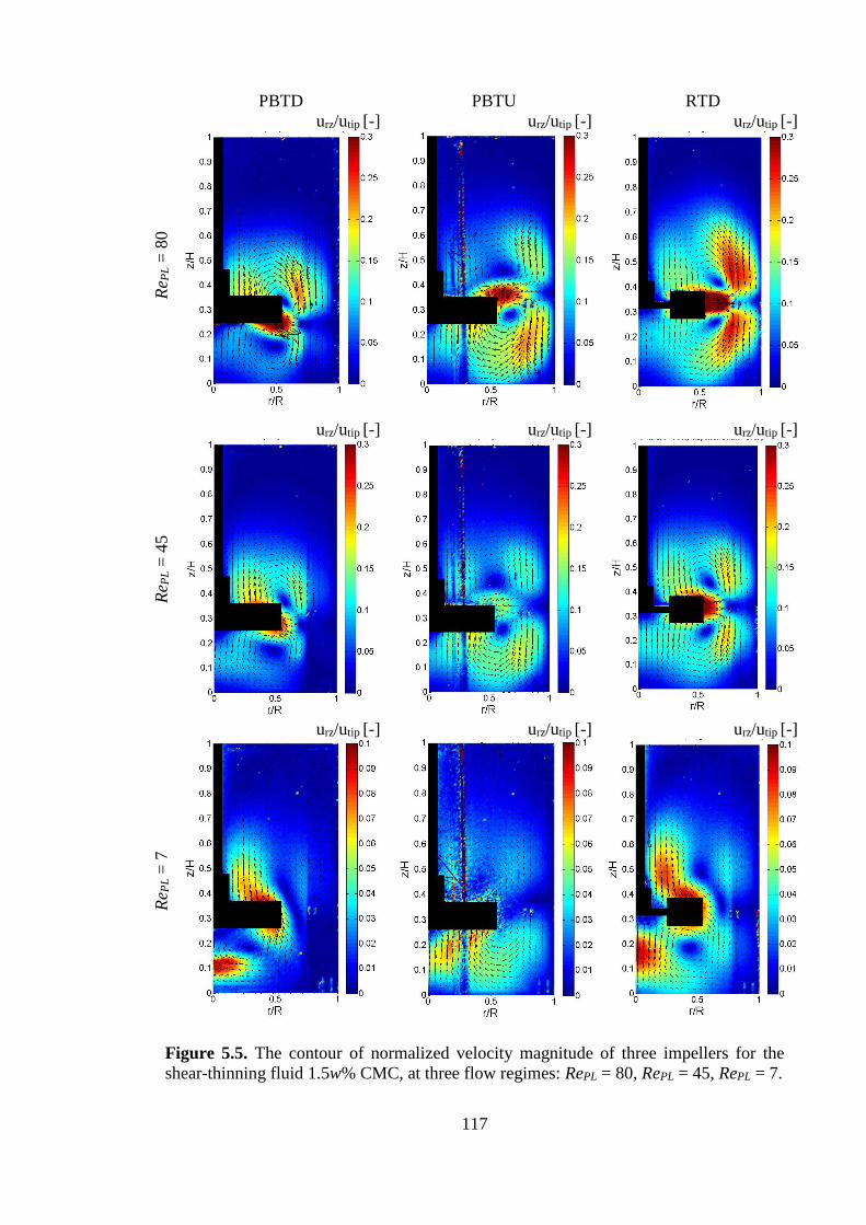
117
Figure 5.5. The contour of normalized velocity magnitude of three impellers for the
shear-thinning fluid 1.5w% CMC, at three flow regimes: RePL = 80, RePL = 45, RePL = 7.
PBTD PBTU RTD
Re P
L =
80
urz/utip [-]
urz/utip [-]
urz/utip [-]
Re P
L =
45
urz/utip [-]
urz/utip [-]
urz/utip [-]
Re P
L =
7
urz/utip [-]
urz/utip [-]
urz/utip [-]
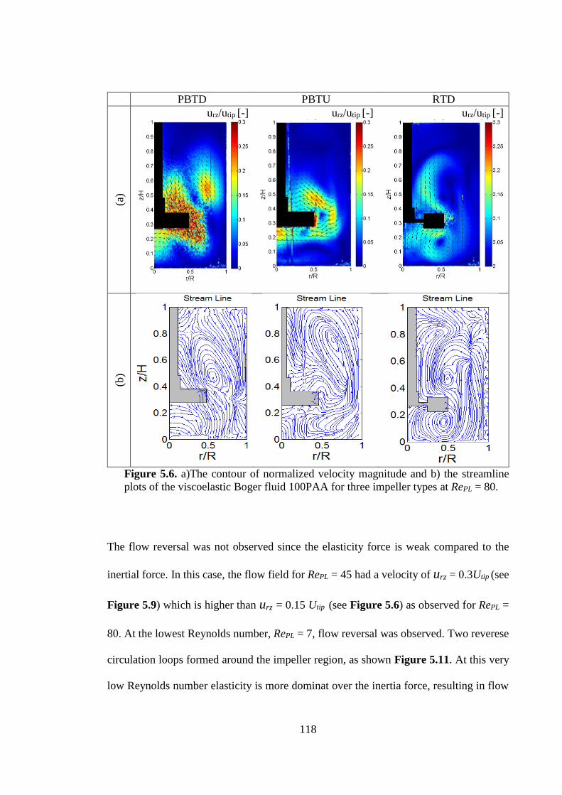
118
PBTD PBTU RTD
(a)
urz/utip [-]
urz/utip [-]
urz/utip [-]
(b)
Figure 5.6. a)The contour of normalized velocity magnitude and b) the streamline
plots of the viscoelastic Boger fluid 100PAA for three impeller types at RePL = 80.
The flow reversal was not observed since the elasticity force is weak compared to the
inertial force. In this case, the flow field for RePL = 45 had a velocity of urz = 0.3Utip (see
Figure 5.9) which is higher than urz = 0.15 Utip (see Figure 5.6) as observed for RePL =
80. At the lowest Reynolds number, RePL = 7, flow reversal was observed. Two reverese
circulation loops formed around the impeller region, as shown Figure 5.11. At this very
low Reynolds number elasticity is more dominat over the inertia force, resulting in flow
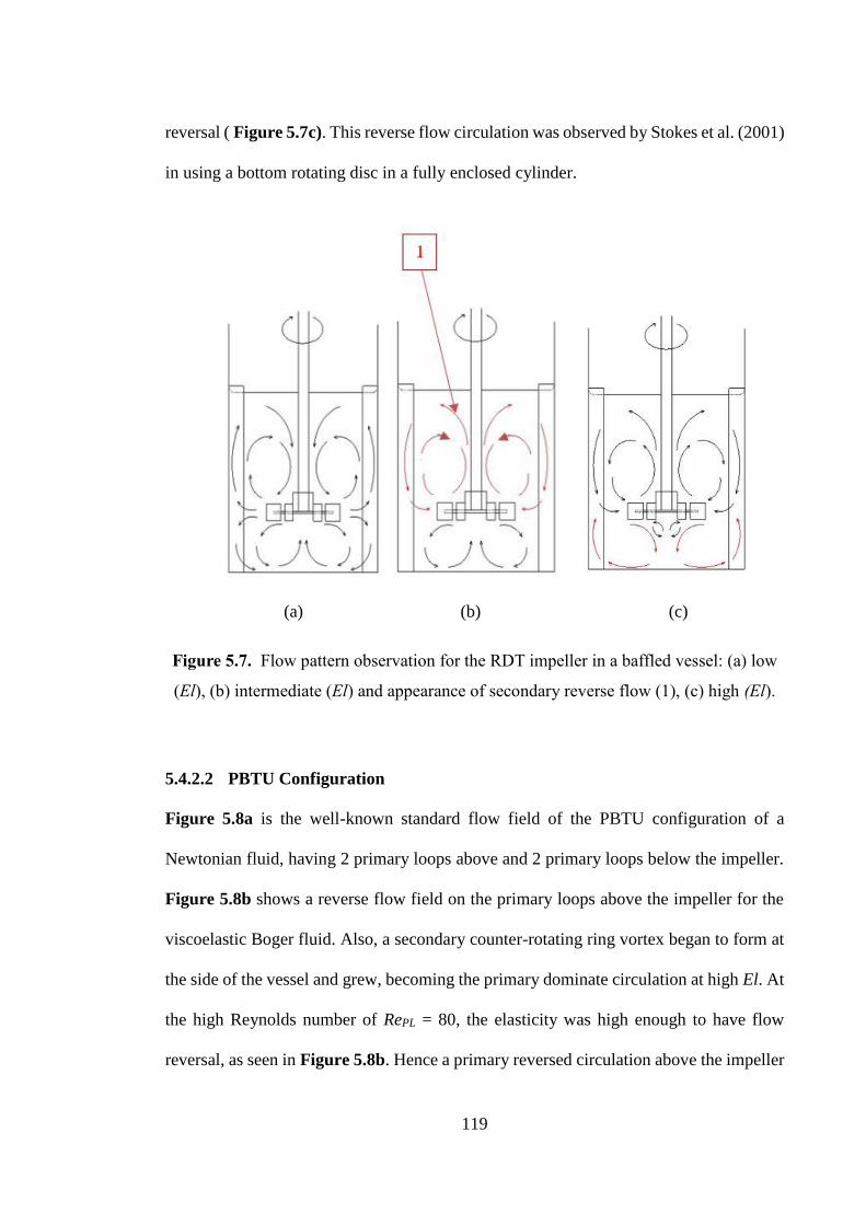
119
reversal ( Figure 5.7c). This reverse flow circulation was observed by Stokes et al. (2001)
in using a bottom rotating disc in a fully enclosed cylinder.
(a) (b) (c)
Figure 5.7. Flow pattern observation for the RDT impeller in a baffled vessel: (a) low
(El), (b) intermediate (El) and appearance of secondary reverse flow (1), (c) high (El).
5.4.2.2 PBTU Configuration
Figure 5.8a is the well-known standard flow field of the PBTU configuration of a
Newtonian fluid, having 2 primary loops above and 2 primary loops below the impeller.
Figure 5.8b shows a reverse flow field on the primary loops above the impeller for the
viscoelastic Boger fluid. Also, a secondary counter-rotating ring vortex began to form at
the side of the vessel and grew, becoming the primary dominate circulation at high El. At
the high Reynolds number of RePL = 80, the elasticity was high enough to have flow
reversal, as seen in Figure 5.8b. Hence a primary reversed circulation above the impeller
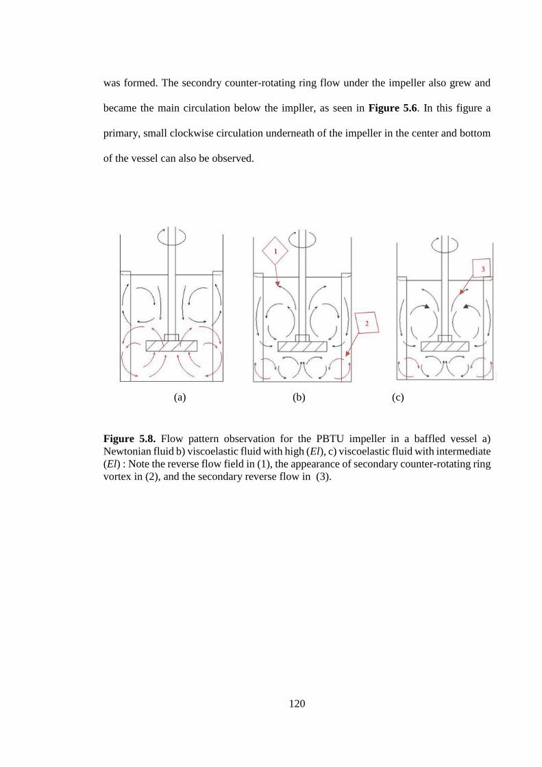
120
was formed. The secondry counter-rotating ring flow under the impeller also grew and
became the main circulation below the impller, as seen in Figure 5.6. In this figure a
primary, small clockwise circulation underneath of the impeller in the center and bottom
of the vessel can also be observed.
(a) (b) (c)
Figure 5.8. Flow pattern observation for the PBTU impeller in a baffled vessel a)
Newtonian fluid b) viscoelastic fluid with high (El), c) viscoelastic fluid with intermediate
(El) : Note the reverse flow field in (1), the appearance of secondary counter-rotating ring
vortex in (2), and the secondary reverse flow in (3).
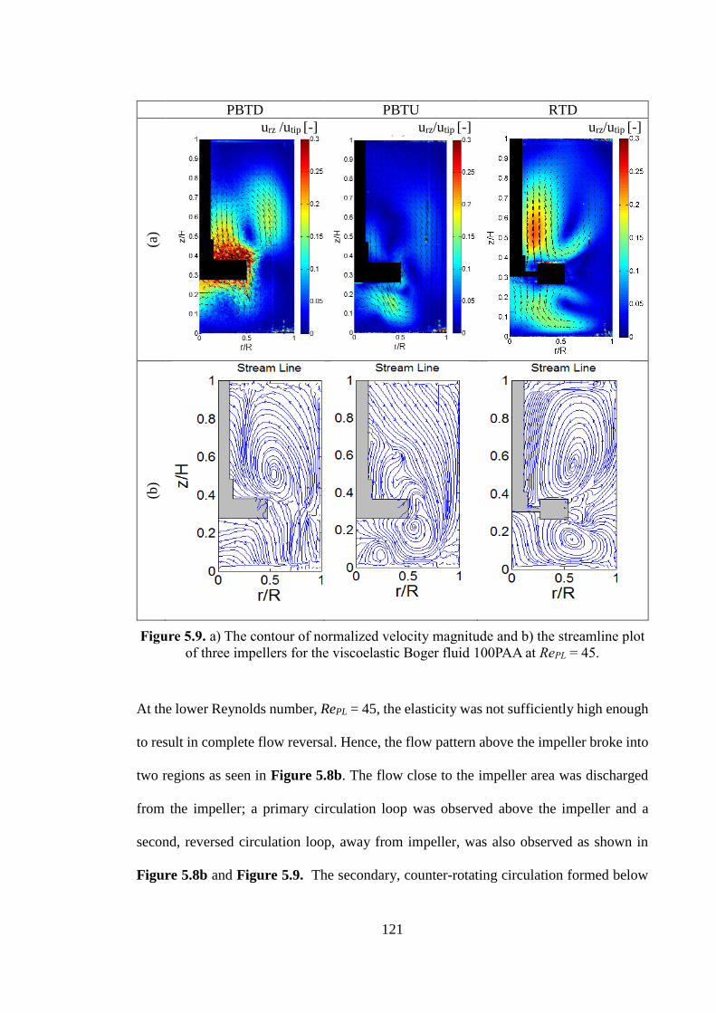
121
PBTD PBTU RTD
(a)
urz /utip [-]
urz/utip [-]
urz/utip [-]
(b)
Figure 5.9. a) The contour of normalized velocity magnitude and b) the streamline plot
of three impellers for the viscoelastic Boger fluid 100PAA at RePL = 45.
At the lower Reynolds number, RePL = 45, the elasticity was not sufficiently high enough
to result in complete flow reversal. Hence, the flow pattern above the impeller broke into
two regions as seen in Figure 5.8b. The flow close to the impeller area was discharged
from the impeller; a primary circulation loop was observed above the impeller and a
second, reversed circulation loop, away from impeller, was also observed as shown in
Figure 5.8b and Figure 5.9. The secondary, counter-rotating circulation formed below
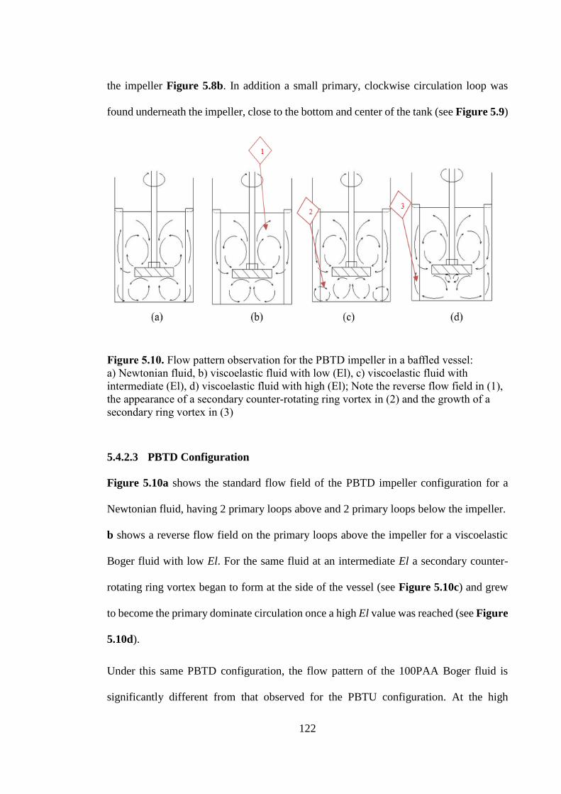
122
the impeller Figure 5.8b. In addition a small primary, clockwise circulation loop was
found underneath the impeller, close to the bottom and center of the tank (see Figure 5.9)
Figure 5.10. Flow pattern observation for the PBTD impeller in a baffled vessel:
a) Newtonian fluid, b) viscoelastic fluid with low (El), c) viscoelastic fluid with
intermediate (El), d) viscoelastic fluid with high (El); Note the reverse flow field in (1),
the appearance of a secondary counter-rotating ring vortex in (2) and the growth of a
secondary ring vortex in (3)
5.4.2.3 PBTD Configuration
Figure 5.10a shows the standard flow field of the PBTD impeller configuration for a
Newtonian fluid, having 2 primary loops above and 2 primary loops below the impeller.
b shows a reverse flow field on the primary loops above the impeller for a viscoelastic
Boger fluid with low El. For the same fluid at an intermediate El a secondary counter-
rotating ring vortex began to form at the side of the vessel (see Figure 5.10c) and grew
to become the primary dominate circulation once a high El value was reached (see Figure
5.10d).
Under this same PBTD configuration, the flow pattern of the 100PAA Boger fluid is
significantly different from that observed for the PBTU configuration. At the high
123
Reynolds number of RePL = 80 the elasticity was high enough to allow for flow reversal
(see Figure 5.10b and Figure 5.6 ). The flow induced by the impeller mostly left it at an
angle of 45o. The primary clockwise circulation below the impeller was observed for the
100PAA Boger fluid in the PBTD configuration. The flow pattern for this fluid remained
relatively the same for the three studied flow regions when using the PBTD impeller
configuration.
5.4.3 High viscoelastic Boger Fluid (300PAA)
Figure 5.12 shows the contour of normalized velocity magnitude of the 300PAA Boger
fluid for the three flow regimes of interest: RePL = 80, RePL = 45 and RePL = 7. The flow
field of this highly viscoelastic fluid - having El = 0.105 at RePL = 80, El = 0.114 at
RePL = 45 and El = 0.169 at RePL = 7 (Table 5.3) - shows flow reversal under all three
impeller configurations. Here the elasticity force (normal force) produced by the shearing
flow is higher than the force due to fluid inertia. Therefore the flow direction was reversed
(Figure 5.12) compared to what was seen for the Newtonian and shear-thinning fluids.
Under all impeller configurations the reverse circulations formed above and below the
tank. In addition a small, primary circulation, just below the impeller and in the center of
the tank, was observed in both PBT impeller configurations at RePL = 80 and RePL = 45.
Moreover, a climbing eddy motion around the shaft was formed due to the presence of
normal forces in the viscoelastic fluid. Comparisons between flow patterns of all test
fluids used in this study under all three impeller configurations at RePL = 80 and RePL =
45 are presented by streamline plots, as shown in Figure 5.13 and Figure 5.14.
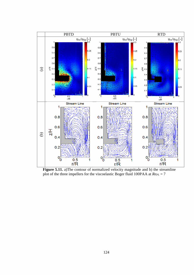
124
PBTD PBTU RTD
(a)
urz/utip [-]
urz/utip [-]
urz/utip [-]
(b)
Figure 5.11. a)The contour of normalized velocity magnitude and b) the streamline
plot of the three impellers for the viscoelastic Boger fluid 100PAA at RePL = 7
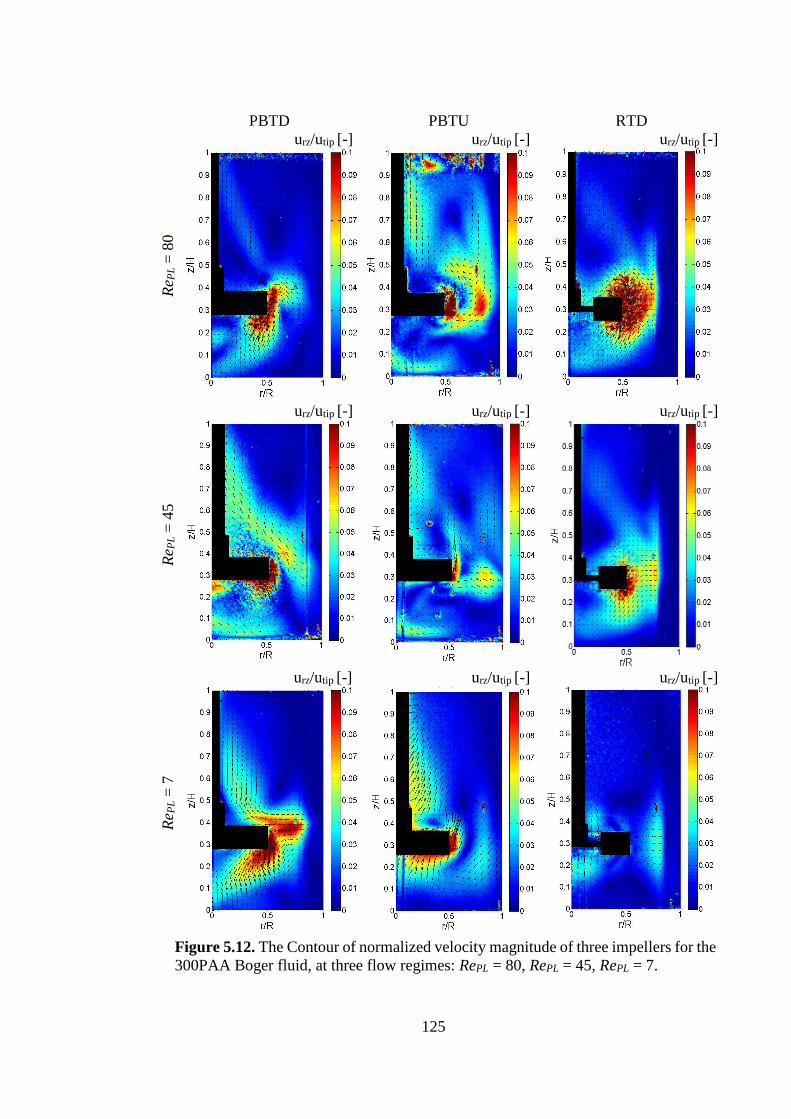
125
PBTD PBTU RTD
Re P
L =
80
urz/utip [-]
urz/utip [-]
urz/utip [-]
Re P
L =
45
urz/utip [-]
urz/utip [-]
urz/utip [-]
Re P
L =
7
urz/utip [-]
urz/utip [-]
urz/utip [-]
Figure 5.12. The Contour of normalized velocity magnitude of three impellers for the
300PAA Boger fluid, at three flow regimes: RePL = 80, RePL = 45, RePL = 7.
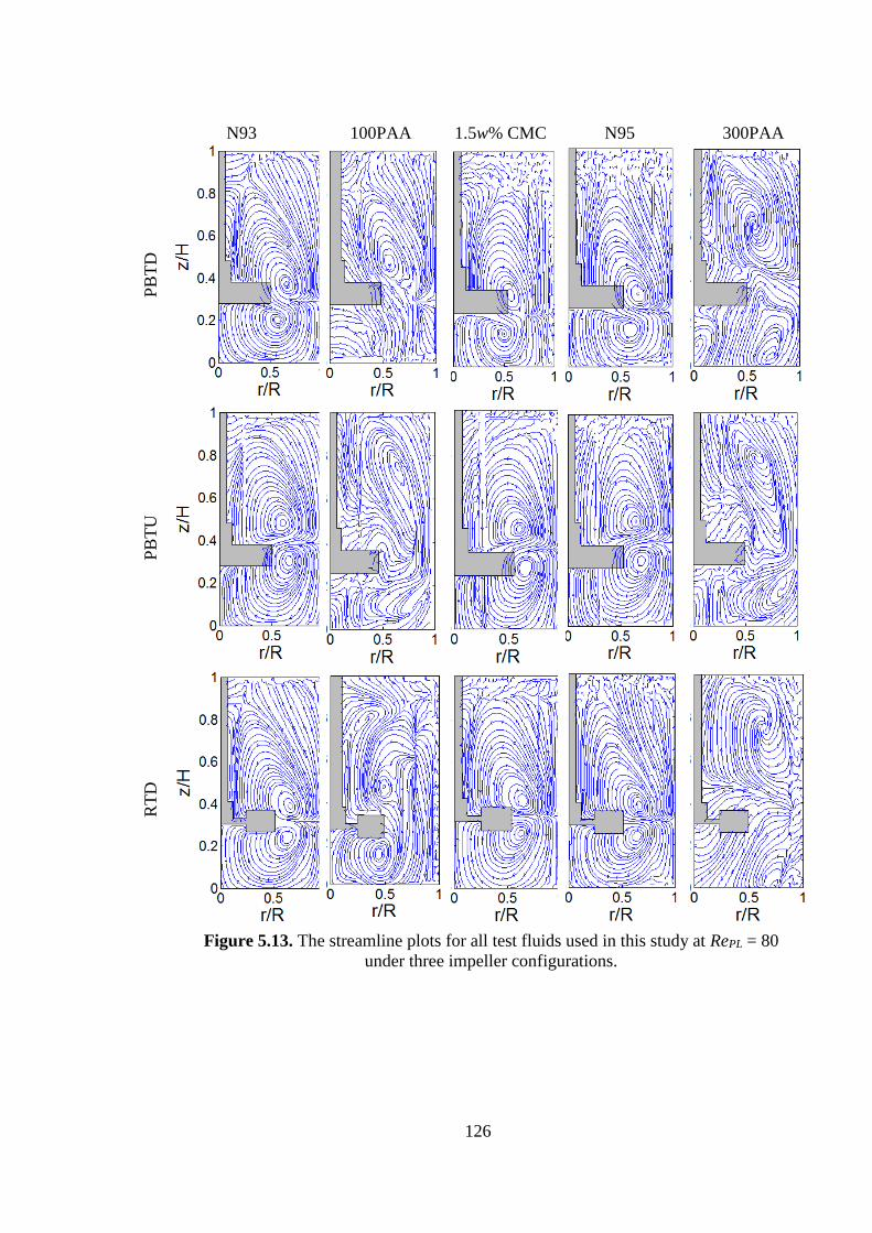
126
N93 100PAA 1.5w% CMC N95 300PAA P
BT
D
PB
TU
RT
D
Figure 5.13. The streamline plots for all test fluids used in this study at RePL = 80
under three impeller configurations.
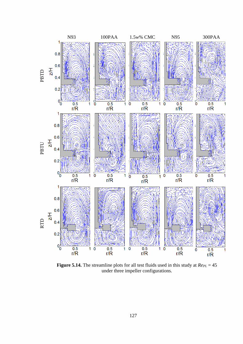
127
N93 100PAA 1.5w% CMC N95 300PAA P
BT
D
PB
TU
RT
D
Figure 5.14. The streamline plots for all test fluids used in this study at RePL = 45
under three impeller configurations.
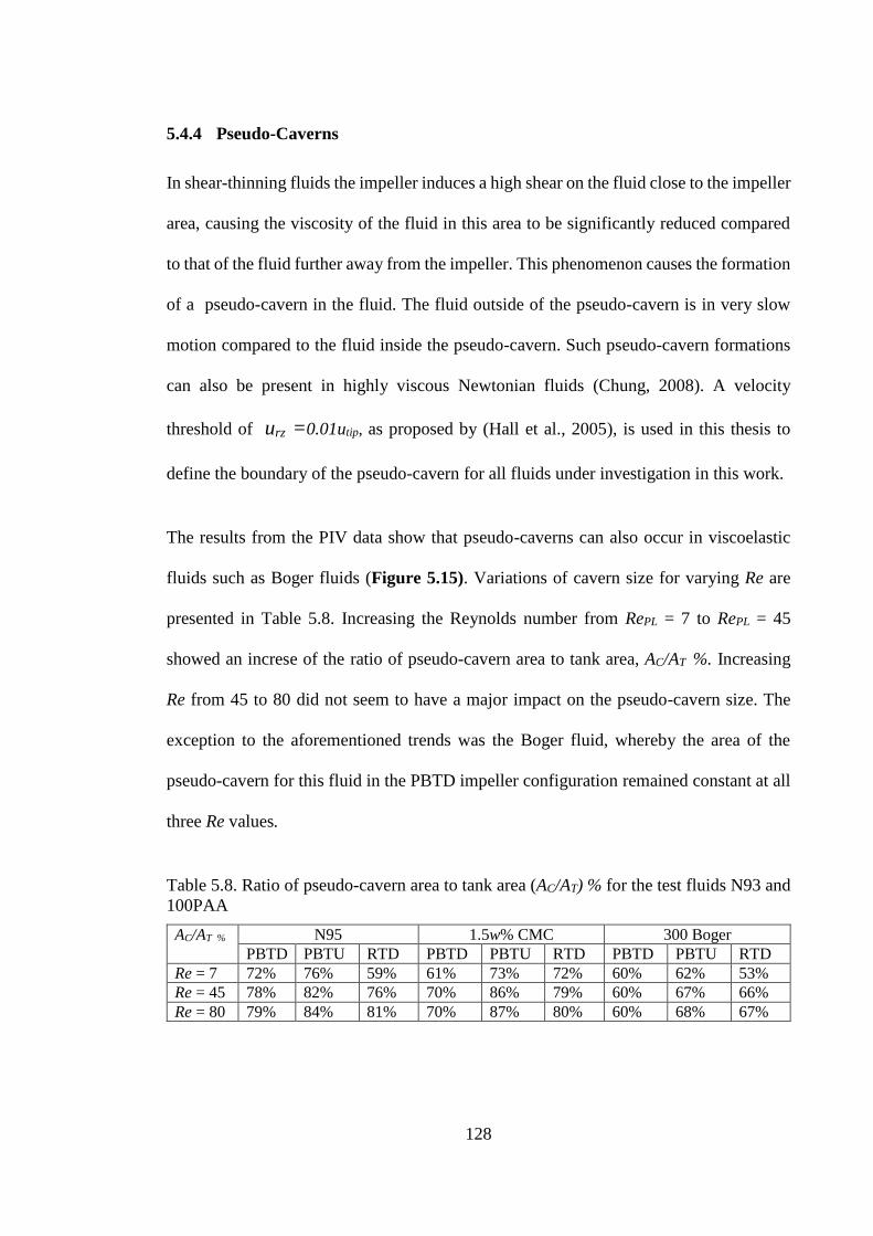
128
5.4.4 Pseudo-Caverns
In shear-thinning fluids the impeller induces a high shear on the fluid close to the impeller
area, causing the viscosity of the fluid in this area to be significantly reduced compared
to that of the fluid further away from the impeller. This phenomenon causes the formation
of a pseudo-cavern in the fluid. The fluid outside of the pseudo-cavern is in very slow
motion compared to the fluid inside the pseudo-cavern. Such pseudo-cavern formations
can also be present in highly viscous Newtonian fluids (Chung, 2008). A velocity
threshold of urz =0.01utip, as proposed by (Hall et al., 2005), is used in this thesis to
define the boundary of the pseudo-cavern for all fluids under investigation in this work.
The results from the PIV data show that pseudo-caverns can also occur in viscoelastic
fluids such as Boger fluids (Figure 5.15). Variations of cavern size for varying Re are
presented in Table 5.8. Increasing the Reynolds number from RePL = 7 to RePL = 45
showed an increse of the ratio of pseudo-cavern area to tank area, AC/AT %. Increasing
Re from 45 to 80 did not seem to have a major impact on the pseudo-cavern size. The
exception to the aforementioned trends was the Boger fluid, whereby the area of the
pseudo-cavern for this fluid in the PBTD impeller configuration remained constant at all
three Re values.
Table 5.8. Ratio of pseudo-cavern area to tank area (AC/AT) % for the test fluids N93 and
100PAA
AC/AT % N95 1.5w% CMC 300 Boger
PBTD PBTU RTD PBTD PBTU RTD PBTD PBTU RTD
Re = 7 72% 76% 59% 61% 73% 72% 60% 62% 53%
Re = 45 78% 82% 76% 70% 86% 79% 60% 67% 66%
Re = 80 79% 84% 81% 70% 87% 80% 60% 68% 67%
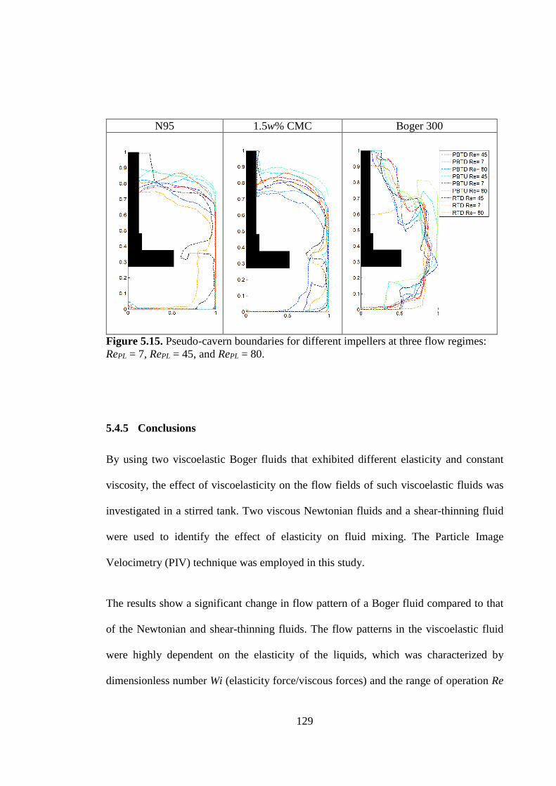
129
N95 1.5w% CMC Boger 300
Figure 5.15. Pseudo-cavern boundaries for different impellers at three flow regimes:
RePL = 7, RePL = 45, and RePL = 80.
5.4.5 Conclusions
By using two viscoelastic Boger fluids that exhibited different elasticity and constant
viscosity, the effect of viscoelasticity on the flow fields of such viscoelastic fluids was
investigated in a stirred tank. Two viscous Newtonian fluids and a shear-thinning fluid
were used to identify the effect of elasticity on fluid mixing. The Particle Image
Velocimetry (PIV) technique was employed in this study.
The results show a significant change in flow pattern of a Boger fluid compared to that
of the Newtonian and shear-thinning fluids. The flow patterns in the viscoelastic fluid
were highly dependent on the elasticity of the liquids, which was characterized by
dimensionless number Wi (elasticity force/viscous forces) and the range of operation Re
130
(inertial force/viscous force). The dimensionless Elastic Number (El=Wi/Re) was applied
to charcterize the strength of the fluid elasticity in a stirred tank and it was able to identify
whether the flow was driven by inertia or elastic forces for each experimental condition.
The Boger fluid 100PAA at a high Reynolds number of RePL = 80, with low elasticity (El
= 0.019) and under the PBTD impeller configuration showed an anti-clockwise
circulation loop above the impeller, similar to that seen in the examined Newtonian and
shear-thinning fluids. However, under the PBTU configuration, the elasticity of the
Boger fluid 100PAA caused the flow circulation loop to become reversed above and
below the impeller. Under the RTD configuration the flow pattern of 100PAA broke into
two regions. The flow close to the impeller area formed two circulation loops above and
below the impeller, with a second reversed circulation loop being formed away from
impeller. The formation of this second loop is undesirable as it leads to the reduction of
mixing efficiency.
At lower flow regimes (RePL = 45, RePL = 7) the viscoelastic fluid behaves like the
Newtonian fluid N93 and the shear-thinning fluid 1.5w% CMC under the RTD and PBD
impeller configurations. The highly viscoelastic Boger fluid 300PAA revealed flow
reversal in both circulations, below and above the impeller within the stirred tank, at all
three flow regimes and under all three impeller types of this study. In this case, the
elasticity force produced by the shearing flow is higher than the force due to fluid inertia,
leading to a reversal of flow direction. The flow velocity is mostly in the tangential
direction, and the time-averaged mean velocity acquired from the PIV data hardly reached
urz = 0.2 Utip in the 300PAA Boger fluid.
131
6 Chapter 6
CONCLUSIONS AND FUTURE WORK
The detailed conclusions for the work presented in this thesis can be found at the end of
each results chapter. This final chapter presents a summary of the overall conclusions and
also recommendations for further research in this area.
6.1 Conclusions
The rheological effects of complex fluids on mixing in a mechanically agitated stirred
vessel were investigated by use of a two-dimensional visualisation technique. 2D Particle
Image Velocimetry (PIV) was employed to characterize the flow fields of a thixotropic
fluid and viscoelastic fluids under laminar and transitional regimes at three different
Reynolds number. The Planar Laser Induced Fluorescence (PLIF) visualization technique
was also applied to the thixotropic fluid in order to investigate in more detail the evolution
of the cavern formation and mixing with time. Three different types of impeller were
investigated in this study: Rushton turbine (RTD), and Pitch Blade Turbine (PBT) in up
pumping mode (PBTU) and in down pumping mode (PBTD).
6.1.1 Effect of Thixotropy on Fluid Mixing in a Stirred Tank
The effects of time dependency were investigated for the mixing of a thixotropic liquid
in a stirred vessel. To investigate only the effect of thixotropy on mixing, other
rheological variables were fixed by choosing a time-independent reference fluid that had
the same rheological properties as that of the thixotropic fluid, here being a transparent
colloidal dispersion of 2.2w% Laponite. The reference fluid used in this work was a 1w%
132
Carbopol aqueous solution, a time-independent, shear-thinning fluid with a yield stress.
Flow fields, flow patterns, normalized mean velocity and cavern growth in the vessel
were characterized during mixing for the thixotropic fluid and the results were compared
to the reference fluid under laminar and transitional regimes at three different Reynolds
number (7, 61 and 158). The mixing efficiency of the impellers was analyzed in terms of
size and growth of a cavern over time and impeller pumping efficiency. Mixing was
performed for 300s.The results show that for both PBTD and PBTU the flow developed
with time and reached a steady state condition almost in the middle of stirring (at t =138s).
For the RTD impeller, the flow fields of the thixotropic fluid reached the steady state
condition early, within t = 14s of mixing. Furthermore, the presence of baffles within the
stirring vessel was also investigated for three impellers (PBTU, PBTD, and RTD). For
the thixotropic fluid in a baffled vessel, the cavern size become larger and improved flow
fields were obtained compared to an un-baffled case at ReHB =158. For the viscoplastic
fluid, the conventional baffled vessel reduced the mixing efficiency by minimizing cavern
size and flow velocity. To conclude, at ReHB =158 in a baffled vessel the yield stress and
apparent viscosity of the studied thixotropic fluid appeared to decline with time during
stirring, indicating that the energy supplied to the fluid is mostly consumed to divert the
flow from a tangential direction to an axial one. For the viscoplastic fluid, the yield stress
acted as a barrier to the fluid momentum.
6.1.2 The Effect Of Viscoelasticity In a Stirred Tank
The mixing of viscoelastic fluids is commonly carried out in stirred tanks in many
industrial processes. To investigate the effect of viscoelasticity on mixing, a model fluid
called Boger was used in this study. This model fluid exhibited constant viscosity over
133
shear, and was prepared by adding polyacrylamide to a viscous, Newtonian fluid. Hence,
the effect of viscoelasticity can be studied in the absence of other rheological behaviors
of most viscoelastic fluids, such as e.g. shear-thinning. The results were compared with
those of a shear-thining fluid, 1.5w% CMC, and viscous Newtonian fluids (glycerin-water
mixes), under laminar and transition regimes at three different Reynolds number (7, 45
and 80) for three type of impellers (PBTU, PBTD, and RTD).
The 2D Particle Image Velocimetry (PIV) technique was used to measure the flow
velocity of the viscoelastic fluid in the mechanically agitated vessel. The flow patterns
for this fluid were highly dependent on the elasticity of the liquid, the latter of which
which was characterized by the dimensionless parameter called the elasticity force, Wi,
and also by the range of operation, Re (inertial force/viscous force). The impeller type
also impacts on the flow behaviour of a viscoelastic Boger fluid with low elasticity.
Moreover, a different flow pattern was observed for each impeller and flow regime.
However, for a viscoelastic Boger fluid with high elasticity a flow reversal was observed
at the three flow regimes and for all three impeller types.
6.2 Future work
In this work, the effect of thixotropy on mixing in stirred vessel was investigated for a
single phase fluid. In a thixotropic fluid the cavern grows with time and even at high
transition Reynold’s number the cavern completely fills the vessel, as opposed to what
happesn with a time-independent fluid with yield stress. As such it is worth investigating
the effect of particle suspensions in mixing of thixotropic fluids with different solid
concentrations and compare results to a reference fluid, both experimentally and
numerically. In addition, the same can be done for particle suspensions in viscoelastic
134
Boger fluids, owing to the fact that particle suspensions within such fluids are commonly
observed in industrial mixing processes.
The behaviour of the viscoelastic Boger fluids used in the work presented here was
investigated with the 2D PIV visualisation technique, in order to better understand the
effect of viscoelasticity on mixing in a stirred vessel. As the flow of such fluids is
observed moving extremely in the tangential direction, it is worth using a non-invasive
technique (such as PEPT) for the analysis of a full 3D velocity field. Fianlly, the capability
of modeling suspensions of particles in viscoelastic Boger fluids can be assessed in
comparison with the PEPT and PIV measurements.
135
7 REFERENCES
Adams, L., Chiti, F., Guida, A., Jaffer, S., Nienow, A.W. and Barigou, M. (2008),
Positron emission particle tracking caverns formed during mixing of an industrial slurry,
Proceedings of International Symposium on Mixing in Industrial Processes VI, Niagara
on the Lake, Niagara Falls, Ontario, Canada, Aug, 17-21.
Adams, L.W. (2009), Experimental and computational study of non-turbulent flow
regimes and cavern formation of non-Newtonian fluids in a stirred tank, Ph.D. Thesis,
University of Birmingham.
Adams, L.W. and Barigou, M. (2007), CFD analysis of caverns and pseudo-caverns
developed during mixing of non-Newtonian fluids, Chemical Engineering Research and
Design, 85 (A5), 598-604.
Adrian, R.J. (1991), Particle-Imaging Techniques for Experimental Fluid-Mechanics,
Annu Rev Fluid Mech, 23(21), 261-304.
Alvarez-Hernández, M.M., Shinbrot, T., Zalc, J. and Muzzio, F.J. (2002), Practical
chaotic mixing, Chem Eng Sci, 57(17), 3749-3753.
Amanullah, A., Hjorth, S.A., Nienow, A.W., (1997), Cavern sizes generated in highly
shear thinning viscous fluids by SCABA 3SHP1 impellers, Transactions I.Chem.E.
75(C), 232-238.
Amanullah, A. H., S. A; Nienow, A.W. 1998. A new mathematical model to predict
cavern dimaters in highly shear thining power law liquids using axial flow impellers.
Chemical Enqmeering Science, 53.
Ameur, H. and Bouzit, M. (2012), Mixing in shear thinning fluids, Brazilian Journal
Chemical Engineering, 29 (2), 349-358.
Ameur, H., Bouzit, M. and Helmaoui, M. (2011), Numerical study of fluid flow and
power consumption in a stirred vessel with a SCABA 6SRGT impeller, Chemical Process
Engineering, 32 (4), 351-366.
Armenante, P. M. and Nagamine, E. U. (1998), Effect of low off-bottom impeller
clearance on the minimum agitation speed for complete suspension of solid in stirred
tanks. Chemical Engineering Science, 53, 1757-1775.
136
Armenante, P.M., Luo, C.G., Chou, C.C., Fort, I. and Medek, J. (1997), Velocity profiles
in a closed, unbaffled vessel: comparison between experimental LDV data and numerical
CFD predictions, Chem Eng Sci, 52(20), 3483-3492.
Arratia, P. E., Kukura, J., Lacombe, J. & Muzzio, F. J. 2006. Mixing of shear-thinning
fluids with yield stress in stirred tanks. AIChE Journal, 52, 2310-2322.
Aubin, J., Fletcher, D. F. and Xuereb, C. (2004), Modeling turbulent flow in stirred tank
with CFD: the influence of the modelin approach, turbulence model and numerical
scheme, Experimental Thermal and Fluid Science, 28, 431-445.
Aubin, J., Le Sauze, N., Bertrand, J., Fletcher, D.F. and Xuereb, C. (2004), PIV
measurements of flow in an aerated tank stirred by a down- and an up-pumping axial flow
impeller, Exp Therm Fluid Sci, 28(5), 447-456.
Aubin, J., Naude, I., Bertrand, J. and Xuereb, C. (2000), Blending of Newtonian and
shear-thinning fluids in a tank stirred with a helical screw agitator, Chemical Engineering
Research and Design, Trans IChenE, 78 (A8), 1105-1114.
Baird, Donald G. (2011). Flow behavior of viscoelastic fluids. In AccessScience.
McGraw-Hill Education.
Bakker, A., Myers, K.J., Ward, R.W. and Lee, C.K. (1996), The laminar and turbulent
flow pattern of a pitch blade turbine, Chemical Engineering Research and Design, 74 (A),
485-491.
Baldi, S. and Yianneskis, M. (2003), On the direct measurement of turbulence energy
dissipation in stirred vessels with PIV, Industrial & Engineering Chemistry Research, 42,
7006-7016.
Barigou, M. (2004), Particle tracking in opaque mixing systems: An overview of the
capabilities of PET and PEPT, Chem Eng Res Des, 82(A9), 1258-1267.
Barigou, M., Chiti, F., Pianko-Oprych, P., Guida, A., Adams, L.; Fan, X., Parker, D. J.
and Nienow, A. W. (2009), Using Positron Emission Particle Tracking (PEPT) to study
mixing in stirred vessels: validation and tackling unsolved problems in opaque systems.
Journal of Chemical Engineering of Japan, 42, 829-846.
Barnes, H. (1997). Thixotropy—a review. Journal of Non-Newtonian Fluid Mechanics,
70(1-2), pp.1-33.
Barnes, H.A.; Hutton, J.F. and Walters, K. (1988) An introduction to rheology. Elsevier.
137
Brito-de la Fuente E., Choplin, L. and Tanguy, P. A. (1997), Mixing with helical ribbon
impellers: effect of highly shear thinning behaviour and impeller geometry, Transaction
IChemE, 75 (A), 45-52.
Bujalski, W., Nienow, A.W. and Liu, H.X. (1990), The Use of Upward Pumping 45-
Degrees Pitched Blade Turbine Impellers in 3-Phase Reactors, Chem Eng Sci, 45(2), 415-
421.
Boger, D. V. & Nguyen, H. 1978. A model viscoelastic fluid. Polymer Engineering &
Science, 18, 1037-1043.
Bonn, D., Tanase, S., Abou, B., Tanaka, H. & Meunier, J. 2002. Laponite: Aging and
Shear Rejuvenation of a Colloidal Glass. Physical Review Letters, 89.
Cabaret, F., Bonnot, S., Fradette, L. and Tanguy, P.A. (2007), Mixing time analysis using
colorimetric methods and image processing, Ind Eng Chem Res, 46(14), 5032-5042.
Choplin, L. & Carreau, P. J. 1986. End effects for highly elastic-constant viscosity fluids.
Rheologica Acta, 25, 95-101.
Chung, K.H.K. (2008), Mixing in high throughput experimentation reactors, Ph.D.
Thesis, University of Birmingham.
Chung, K.H.K., Barigou, M. and Simmons, M.J.H. (2007), Reconstruction of 3-D flow
field inside miniature stirred vessels using a 2-D PIV technique, Chemical Engineering
Research and Design, 85 (A5), 560-567.
Chung, K.H.K., Simmons, M.J.H. and Barigou, M. (2009), Angle-resolved Particle Image
Velocimetry measurements of flow and turbulence fields in small-scale stirred vessels of
different mixer configurations, Ind Eng Chem Res, 48(2), 1008-1018.
Cronin, D.G., Nienow, A.W. and Moody, G.W. (1994), An experimental study of the
mixing in a protofermenter agitated by dual Rushton turbines, Food Bioprod Process,
72(C1), 35-40.
Collias, D. J. & Prud'homme, R. K. 1985. The effect of fluid elasticity on power
consumption and mixing times in stirred tanks. Chemical Engineering Science, 40, 1495-
-1505.
Couerbe, G., Fletcher, D. F., Xuereb, C. & Poux, M. 2008. Impact of thixotropy on flow
patterns induced in a stirred tank: Numerical and experimental studies. Chemical
Engineering Research and Design, 86, 545-553.
138
Coussot, P., Leonow, A. I. & Piau, J. M. 1993. Rheology of concentrated dispersed
systems in a low molecular weight matrix. Journal of Non-Newtonian Fluid Mechanics,
46, 179-217.
Coussot, P., Nguyen, Q. D., Huynh, H. T. & Bonn, D. 2002. Avalanche Behavior in Yield
Stress Fluids. Physical Review Letters, 88.
Cutter, L.A. (1966), Turbulence: The filtering approach, Journal of Fluid Mechanics, 238,
325-336.
Derksen, J. J. 2010. Agitation and mobilization of thixotropic liquids. AIChE Journal,
56(9), 2236-2247.
Edwards, M.F., Baker, M.R. and Godfrey, J.C. (1997), Laminar flow and distributive
mixing, in: Harnby, N., Edwards, M.F., Nienow, A.W. (Eds), Mixing in the process
industries, Butterworth-Heinemann: Oxford. Chapter 11, 200-224.
Ein-Mozaffari, F., Upreti, S.R. (2009), Using ultrasonic Doppler velocimetry and CFD
modelling to investigate the mixing of non-Newtonian fluid possessing yield stress,
Chemical Engineering Research and Design, 87, 515-523.
Escudié, R. and Liné, A. (2006), Analysis of turbulence anisotropy in a mixing tank,
Chemical Engineering Science, 61 (9), 2771-2779.
Escudie, R., Bouyer, D., Line, A., 2004. Characterization of trailing vortices generated
by a Rushton turbine. A.I.Ch.E. Journal 50, 75.
Fairhurst, P.G., Barigou, M., Fryer, P.J., Pain, J-P., Parker, D.J., (2001), Using positron
emission particle tracking (PEPT) to study nearly neutrally buoyant particles in high solid
fraction pipe flow, International Journal of Multiphase Flow, 27, 1881-1901.
Fangary, Y.S., Barigou, M., Seville, J.P.K. and Parker, D.J. (2000), Fluid trajectories in
a stirred vessel of non-Newtonian liquid using Positron Emission Particle Tracking,
Chemical Engineering Science, 55 (24), 5969-5979.
Fangary, Y.S., Barigou, M., Seville, J.P.K. and Parker, D.J. (2002), A Lagrangian study
of solids suspension in a stirred vessel by Positron Emission Particle Tracking (PEPT),
Chemical Engineering Technology, 25 (5), 521-528.
Fangary, Y.S., Seville, J.P.K. and Barigou, M. (1999), Flow studies in stirred tanks by
positron emission particle tracking (PEPT), Institution of Chemical Engineers
Symposium Series, 146, 23-24.
139
Gabriele, A., Nienow, A.W. and Simmons, M.J.H. (2009), Use of angle resolved PIV to
estimate local specific energy dissipation rates for up- and down-pumping pitched blade
agitators in a stirred tank, Chem Eng Sci, 64(1), 126-143.
Galindo, E. and Nienow, A. W. (1992), Mixing of highly viscous simulated Xanthan
fermentation broths with the Lightinin A-315 impeller, Biotechnology Progress, 8, 233-
239.
Galletti, C., Paglianti, A., Yianneskis, M., (2005), Observations on the significance of
instabilities turbulence and intermittent motions on the fluid mixing processes in stirred
reactors, Chemical Engineering Science, 60, 2317-2331.
Guida, A. (2010), Positron emission particle tracking applied to solid-liquid mixing in
mechanically agitated vessels, Ph.D. Thesis, University of Birmingham.
Guida, A., Nienow, A. W. & Barigou, M. 2010. The effects of the azimuthal position of
the measurement plane on the flow parameters determined by PIV within a stirred vessel.
Chemical Engineering Science, 65, 2454-2463.
Guillard, F., Trägärdh, C. and Fuchs, L. (2000), A study of turbulent mixing in a turbine-
agitated tank using a fluorescence technique, Experiments in Fluids, 28, 225-235.
Gunkel, A.A., Weber, M.E., 1975, Flow phenomena in stirred tanks, Part I. The impeller
stream, A.I.Ch.E. Journal, 21(5), 931-948.
Hall, J.F., Barigou, M., Simmons, M.J.H. and Stitt, E.H. (2005a), Just because it's small
doesn't mean it's well mixed: Ensuring good mixing in mesoscale reactors, Ind Eng Chem
Res, 44(25), 9695-9704.
Hall, J.F., Barigou, M., Simmons, M.J.H. and Stitt, E.H. (2005b), Comparative study of
different mixing strategies in small high throughput experimentation reactors, Chem Eng
Sci, 60(8-9), 2355-2368.
Hall, J. J. 2005. Study of viscous and viscoelastic flows with reference to laminar stirred
vessels. Ph.D. Thesis, University of London.
Hirata, Y. & Aoshima, Y. 1996. Formation and growth of cavern in yield stress fluids
agitated under baffled and non-baffled conditions. Chemical engineering research &
design, 74, 438-444.
James, D. F. 2009. Boger Fluids. Annual Review of Fluid Mechanics, 41, 129--142.
140
Jaworski, Z., Nienow, A.W., Koutsakos, E., Dyster, K. and Bujalski, W. (1991), An LDA
study of turbulent flow in a baffled vessel agitated by a pitched blade turbine, Chemical
Engineering Research and Design, 64 (A4), 313-320.
Khan, F. R. 2005. Investigation of turbulent flows and instabilities in a stirred vessel using
particle image velocimetry, Ph.D. Thesis, Loughborough University.
Khan, F. R., Rielly, C. D. and Hargrave, G. D. (2004), A multi-block approach to obtain
angle-resolved PIV measurements of the mean flow and turbulence fields in a stirred
vessel, Chemical Engineering Technology, 27 (3), 264-269.
Khan, F.R., Rielly, C.D. and Brown, D.A.R. (2006), Angle-resolved stereo-PIV
measurements close to a down-pumping pitched-blade turbine, Chemical Engineering
Science, 61 (9), 2799-2806.
Kresta, S.M. and Wood, P.E. (1993), The flow field produced by a pitched blade turbine:
characterization of the turbulence and estimation of the dissipation rate, Chemical
Engineering Science, 48 (10), 1761–1774.
Kukura, J., Arratia, P.C., Szalai, E.S., Bittorf, K.J. and Muzzio, F.J. (2002),
Understanding pharmaceutical flows, Pharmaceutical Technology, 48-72.
Lim, K. S. 2005. Studies of foam microstructure and rheology, Ph.D. Thesis, The
University of Birmingham.
Liu, L. 2013. Computatinal fluid dynamics modeling of complex fluid flow in stirred
vessels, Ph.D. Thesis, The University of Birmingham.
Lourenco, L.M., Krothopalli, A. and Smith, C.A. (1989), Particle image velocimetry, in:
Gad-el-Hak, M. (Ed), Advances in fluid mechanics measurement, Springer-Verlag:
Berlin. Chapter 4, 128-199.
Mackay, M. E. & Boger, D. V. 1987. An explanation of the rheological properties of
Boger fluids. Journal of Non-Newtonian Fluid Mechanics, 22, 235-243.
Magda, J. J., Lou, J., Baek, S. G. & Devries, K. L. 1991. Second normal stress difference
of a Boger fluid. Polymer, 32, 2000--2009.
Maingonnat, J.F., Muller, L., Leuliet, J.C., (2005), Modelling the build-up of a thixotropic
fluid under viscosimetric and mixing conditions, Journal of Food Engineering, 3, 265-
272.
141
Mavros, P., Xuereb, C. and Bertrand, J. (1996), Determination of 3-D flow fields in
agitated vessels by laser-Doppler velocimetry: Effect of impeller type and liquid viscosity
on liquid flow patterns, Chem Eng Res Des, 74(A6), 658-668.
Mavros, P., Xuereb, C. and Bertrand, J. (1998), Determination of 3-D flow fields in
agitated vessels by laser-Doppler velocimetry: Use and interpretation of RMS velocities,
Chem Eng Res Des, 76(A2), 223-233.
Metzner, A.B. and Otto, R.E. (1957), Agitation of Non-Newtonian Fluids, AIChE J, 3(1),
3-10.
Micheletti, M. and Yianneskis, M. (2004), Study of fluid velocity characteristics in stirred
solid-liquid suspensions with a refractive index matching technique, Proceedings of the
Institution of Mechanical Engineers, 218, 191-204.
Montante, G., Lee, K. C., Brucato, A. and Yianneskis, M. (1999), Double to single loop
flow pattern transition in stirred vessels, The Canadian Journal of Chemical Engineering,
77, 649-659.
Montante, G., Paglianti, A. and Magelli, F. (2012), Analysis of dilute solid-liquid
suspensions in turbulent stirred tanks, Chemical Engineering Research and Design, 90
(10), 1448-1456.
Nienow, A.W. (1968), Suspension of Solid Particles in Turbine Agitated Baffled Vessels,
Chem Eng Sci, 23(12), 1453-1459.
Nienow, A.W. (1997a), On impeller circulation and mixing effectiveness in the turbulent
flow regime, Chemical Engineering Science, 52 (15), 2557-2565.
Nienow, A.W. (1997b), The suspension of solids particles, in: Harnby, N., Edwards,
M.F., Nienow, A.W. (Eds), Mixing in the process industries, Butterworth-Heinemann:
Oxford. Chapter 16, 364-394.
Nouri, J. M. & Whitelaw, J. H. 1990. Flow characteristics of stirred reactors with
newtonian and non-newtonian fluids. AIChE Journal, 36, 627-629.
Ochieng, A., Onyango, M.S., Kumar, A., Kiriamiti, K. and Musonged, P. (2008), Mixing
in a tank stirred by a Rushton turbine at a low clearance, Chemical Engineering and
Processing, 47, 842-851.
Özcan-Taskin, N. Gul (1993), On the Effects of Viscoelasticity in Stirred Tanks Ph.D.
Thesis, University of Birmingham.
142
Özcan-Taskin, N. Gul, AW Nienow (1995), Mixing viscoelastic fluids flow with axial
'impellers: flow fields and power consumption, Food and Bioproducts Processing, 73, 49-
56.
Papadopoulos, G. and Arik, E.B. (2004), Experimental Methods: Fundamental Flow
Measurement, in: Paul, E.L., Atiemo-Obeng, V.A. and Kresta, S.M. (Eds), Handbook of
industrial mixing: Science and practice, Wiley- Interscience: Hoboken, NJ. Chapter 4B,
202-256.
Parker, D.J., Broadbent, C.J., Fowles, P., Hawkesworth, M.R. and Mcneil, P. (1993),
Positron Emission Particle Tracking - A technique for studying flow within engineering
equipment, Nucl Instrum Methods Phys Res A, 326(3), 592-607.
Parker, D.J., Forster, R.N., Fowles, P. and Takhar, P.S. (2002), Positron Emission Particle
Tracking using the new Birmingham positron camera, Nucl Instrum Methods Phys Res
A, 477(1-3), 540-545.
Paul, E. L., Atiemo-Obeng, V. A. and Kresta, S. M. (2004), Hand book of industrial
mixing: Science and practice, Wiley-Interscience: Hoboken, NJ.
Peters and Smith, (1962). Chemical Engineering Journal, Volume 8, pp-83.
Pianko-Oprych, P., Nienow, A.W. and Barigou, M. (2009), Positron emission particle
tracking (PEPT) compared to particle image velocimetry (PIV) for studying the flow
generated by a pitched-blade turbine in single phase and multi-phase systems, Chemical
Engineering Science, 64 (23), 4955–4968.
Prajapati, P. and Ein-Mozaffari, F. (2009), CFD investigation of the mixing of yield-
pseudoplastic fluid with anchor impeller, Chemical Engineering, Tecnology, 32 (8),
1211-1218.
Prilutski, G., Gupta, R. K., Sridhar, T. & Ryan, M. E. 1983. Model viscoelastic liquids.
Journal of Non-Newtonian Fluid Mechanics, 12, 233-241.
Pryce-Jones, (1934, 1836, 1943). Journal of the Oil and Colour Chemists' Association.
Wembley, Middlesex, 17 (1934) 305; 19 (1936) 395; 26 (1943) 3.
Rice, M., Hall, J., Papadakis, G. & Yianneskis, M. 2006. Investigation of laminar flow in
a stirred vessel at low Reynolds numbers. Chemical Engineering Science, 61, 2762-2770.
Rutherford, K., Mahmoudi, S.M.S., Lee, K.C. and Yianneskis, M. (1996), The influence
of Rushton impeller blade and disk thickness on the mixing characteristics of stirred
vessels, Chemical Engineering Research and Design, 74 (A), 369-378.
143
Sano, Y. and Usui, H. (1985), Interrelations among mixing time, power number and
discharge flow rate number in baffled mixing vessels, Journal of Chemical Engineering
of Japan, 18 (1), 47-52.
Seyssiecq, I. & Tolofoudy 2003. Viscoelastic Liquids in Stirred Vessels– Part I: Power
Consumption in Unaerated Vessels. Chemical Engineering \& Technology, 26, 1155--
1165.
Schäfer, M., Yianneskis, M., Wächter, P., Durst, F., 1998, Trailing vortices around a 45°
Pithced-blade impeller, AIChE Journal, 44 (6), 1233-1246.
Scott-Blair, G.W. (1943) A Survey of General and Applied Rheology, London, Pitman.
Seitzman, J.M. and Hanson, R.K. "Planar Fluorescence Imaging in Gases," in
Experimental Methods for Flows With Combustion ed. A. Taylor. Academic Press,
London (1993).
Sharp, K. V. and Adrian, R. J. (2001), PIV study of small-scale flow structure around a
Rushton turbine, Fluid Mechanics and Transport Phenomena, 47 (4), 766-778.
Sheng, J., Meng, H. and Fox, R.O. (1998), Validation of CFD simulations of a stirred
tank using particle image velocimetry data, The Canadian Journal of Chemical
Engineering, 76, 611-625.
Skelland A.H.P. (1967) Non-Newtonian flow and heat transfer. John Wiley and Sons Inc.
New York.
Stokes, J. R. 1998. swirling flow of viscoelstic fluids. Doctor of Philosophy, University
of Melbourne.
Stokes, J. R., Graham, L. J. W., Lawson, N. J. & Boger, D. V. 2001. Swirling flow of
viscoelastic fluids. Part 1. Interaction between inertia and elasticity. Journal of Fluid
Mechanics, 429, 67--115.
Ulbrecht, J.J. and Carreau, P. (1985) Mixing of viscous non-Newtonian liquids (in
'Mixing of liquids by mechanical agitation' Gordon and Breach, New York. eds.
ULBRECHT, J.J. and G.K. PATTERSON) p: 93- 135.
Szalai, E.S., Arratia, P., Johnson, K. and Muzzio, F.J. (2004), Mixing analysis in a tank
stirred with Ekato Intermid®impellers, Chemical Engineering Science, 59, 3793-3805.
Thyagaraja, A., Fletcher, D. and Cook, I. (1987). One-dimensional calculations of two-
phase mixing flows. International Journal for Numerical Methods in Engineering, 24(2),
pp.459-469.Turbine Impellers in 3-Phase Reactors, Chem Eng Sci, 45(2), 415-421.
144
Unadkat, H., Rielly, C.D. and Hargrave, G.K. (2009), Application of fluorescent PIV and
digital image analysis to measure turbulence properties of solid-liquid stirred
suspensions, Chemical Engineering Research and Design, 87 (4), 573-586.
Weissenberg, K. (1948), “Abnormal Substances and Abnormal Phenomena of Flow,”
Proc. of First Intl. Cong. Rheol., North Holland, Amsterdam, I29.
Whelan, T. (1994), Polymer Technology Dictionary, Chapman & Hall, London.
Willert, C.E. and Gharib, M. (1991), Digital Particle Image Velocimetry, Exp Fluids,
10(4), 181-193.
Wu, H. and Patterson, G. K. (1989), Laser-Doppler measurements of turbulent-flow
parameters in a stirred mixer, Chemical Engineering Science, 44 (10), 2207-2221.
Yianneskis, M., Popiolek, Z. and Whitelaw, J. H. (1987), An experimental study of the
steady and unsteady flow characteristics of stirred reactors, Journal of Fluid Mechanics,
175,537-555.
Zalc, J. M., Alvarez, M. M., Muzzio, F. J. and Arik, B. E. (2001), Extensive validation of
computed laminar flow in a stirred tank with three Rushton turbines, AIChE Journal, 47
(10), 2145-2154.
Zalc, J. M., Alvarez, M. M., Muzzio, F. J. and Arik, B. E. (2001), Extensive validation of
computed laminar flow in a stirred tank with three Rushton turbines, AIChE Journal, 47
(10), 2145-2154.
Zhou, G. and Kresta, S. M. (1996), Impact of geometry on the maximum turbulence
energy dissipation rate for various impellers, AIChE Journal, 42, 2476-2490.
Zlokarnik, M. (2001), Stirring: Theory and practice, Wiley-VCH: Weinheim.

145