Embed Size (px)
DESCRIPTION
The sampling of continuous-time signals is an important topic. It is required by many important technologies such as:. Digital Communication Systems ( Wireless Mobile Phones, Digital TV (Coming) , Digital Radio etc ). CD and DVD. - PowerPoint PPT Presentation
Citation preview
The sampling of continuous-time signals is an important topic
It is required by many important technologies such as:
Digital Communication Systems ( Wireless Mobile Phones, Digital TV (Coming) , Digital Radio etc )
CD and DVD
Digital Photos
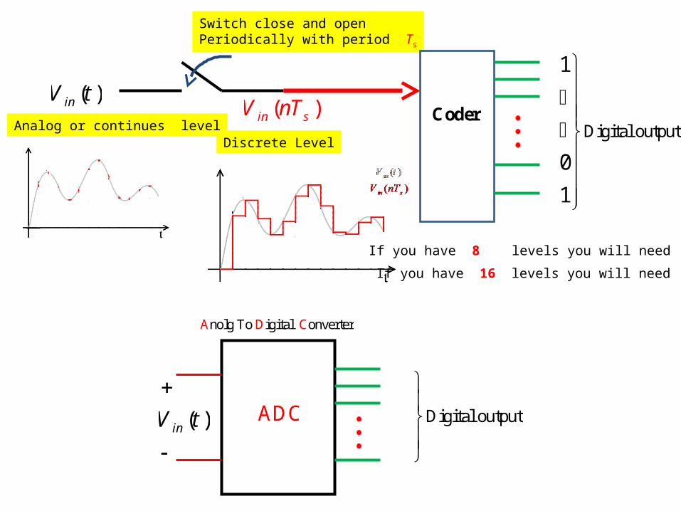
( )inV t
Digital output
nolg To igital onveA D C rter
ADC
( )inV t
Switch close and open Periodically with period Ts
( )in sV nT Coder
Discrete LevelDigital output
1
0
1
If you have 8 levels you will need 3 bits
If you have 16 levels you will need 4 bits
Analog or continues level
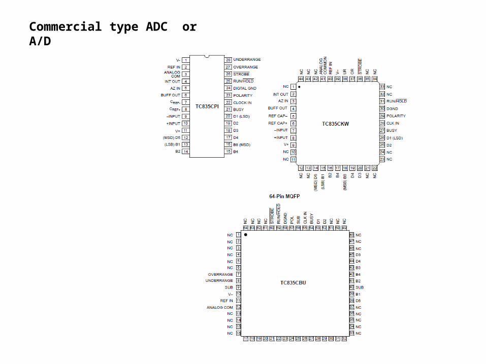
Commercial type ADC or A/D
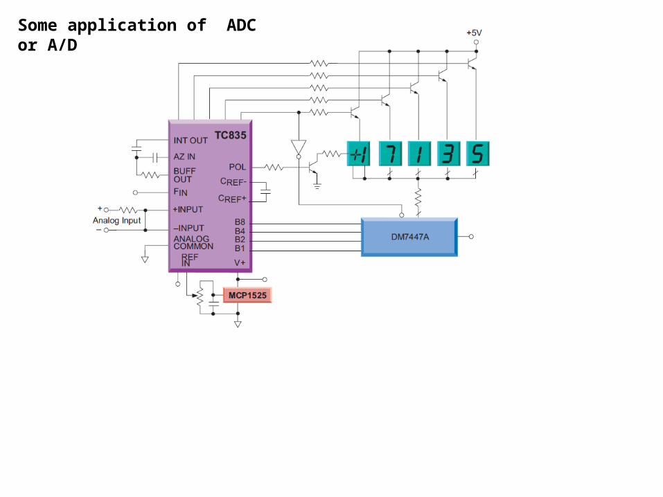
Some application of ADC or A/D

00
0
( )2 ( )
n
G nn
T
0
0
( )n
G nC
T
Recall Fourier Transform of periodical signal
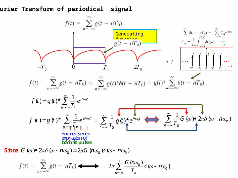
Fourier Transform of periodical signal
00
0
( )2 ( )
n
G nn
T
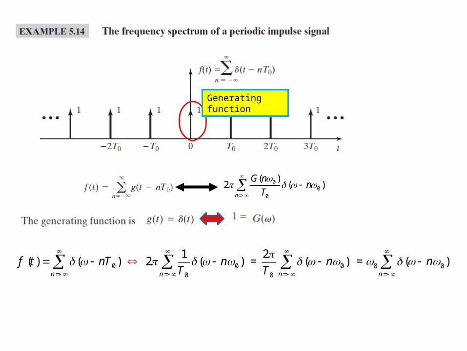
Generating function
0
0
1( ) ( )* jn t
n
f t g t eT
0
0
1= ( )* jn t
n
g t eT
0
0
Fourier Seriesexpnasion of
1( ) ( )* jn t
n
f t g t eT
train impulses
0
0
1( ) 2 ( )
n
G nT
0 0 0 ( ) 2 ( ) 2 ( ) ( )G n G n n Since
Generating function
00
0
( )2 ( )
n
G nn
T
0 00
1( ) ( 2 ( ) )
n n
f t nT nT
00
2= ( )
n
nT
0 0= ( )n
n
Since
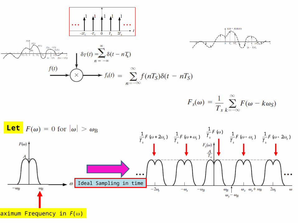
Let
Maximum Frequency in F()
1( 2 )s
s
FT
1( )s
s
FT
1
( )ss
FT
1
( 2 )ss
FT
1( )
s
FT
Ideal Sampling in time
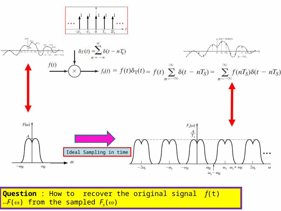
Question : How to recover the original signal f(t) ↔F() from the sampled Fs()
Ideal Sampling in time
Ideal Sampling in time
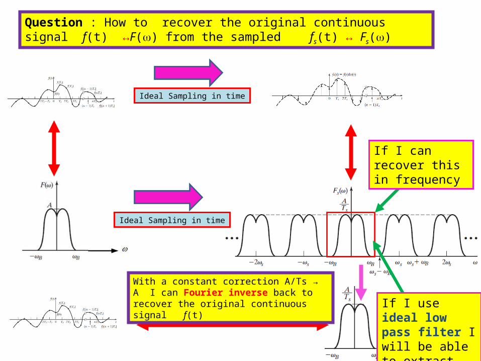
Question : How to recover the original continuous signal f(t) ↔F() from the sampled fs(t) ↔ Fs()
Ideal Sampling in time
If I can recover this in frequency
With a constant correction A/Ts → A I can Fourier inverse back to recover the original continuous signal f(t) If I use ideal low
pass filter I will be able to extract this
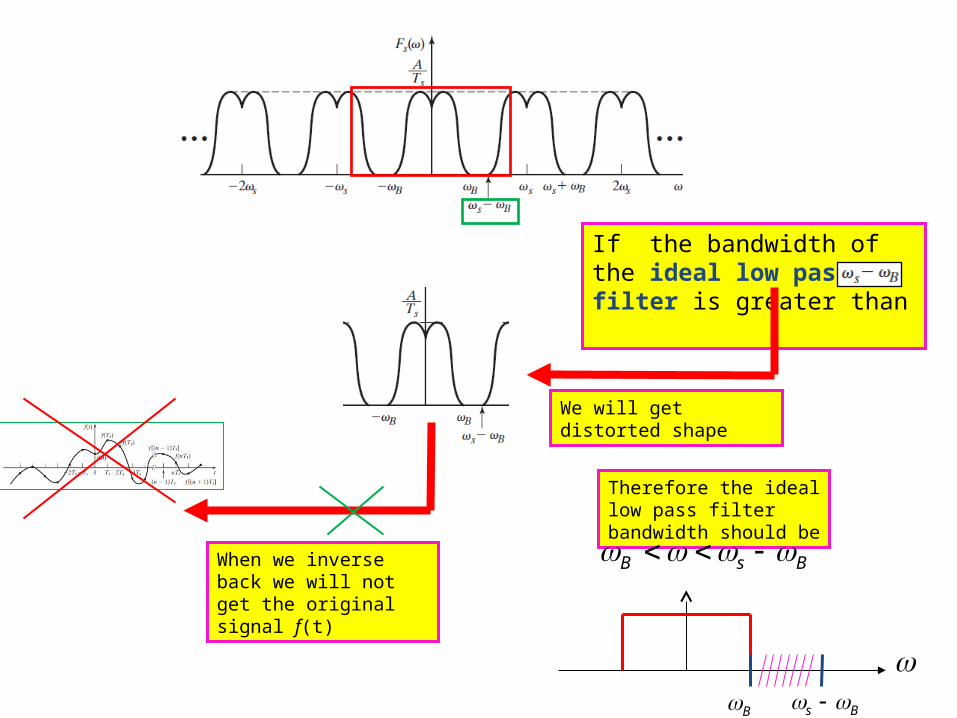
If the bandwidth of the ideal low pass filter is greater than
We will get distorted shape
When we inverse back we will not get the original signal f(t)
Therefore the ideal low pass filter bandwidth should be
B s B
s B B
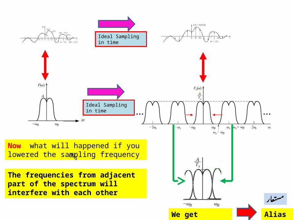
Ideal Sampling in time
Ideal Sampling in time
Now what will happened if you lowered the sampling frequency s
The frequencies from adjacent part of the spectrum will interfere with each other
We get distortion Aliasing
مستعار

http://www.youtube.com/watch?v=pVcuntWruuY&feature=related
http://www.youtube.com/watch?v=jHS9JGkEOmA
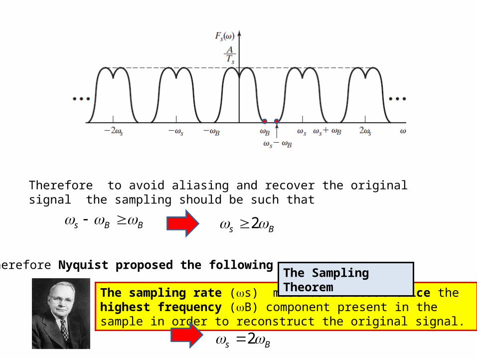
Therefore to avoid aliasing and recover the original signal the sampling should be such that
s B B 2s B
Therefore Nyquist proposed the following
The sampling rate (s) must be at least twice the highest frequency (B) component present in the sample in order to reconstruct the original signal.
2s B
The Sampling Theorem
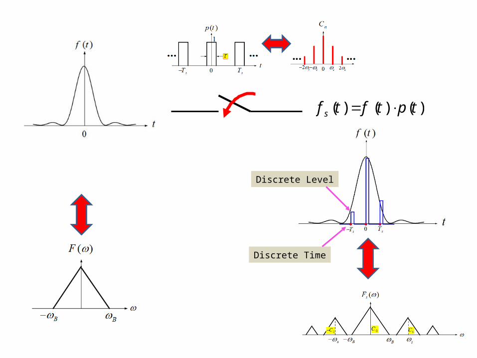
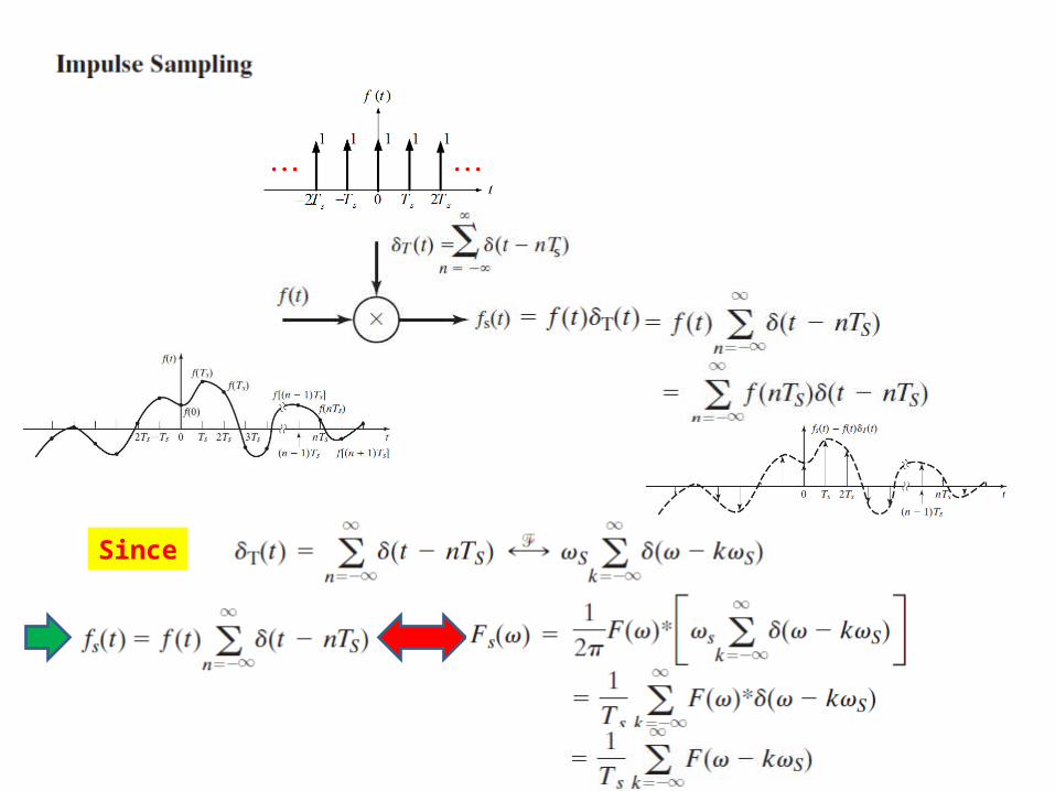
( ) ( ) ( )sf t f t p t
Discrete Time
Discrete Level
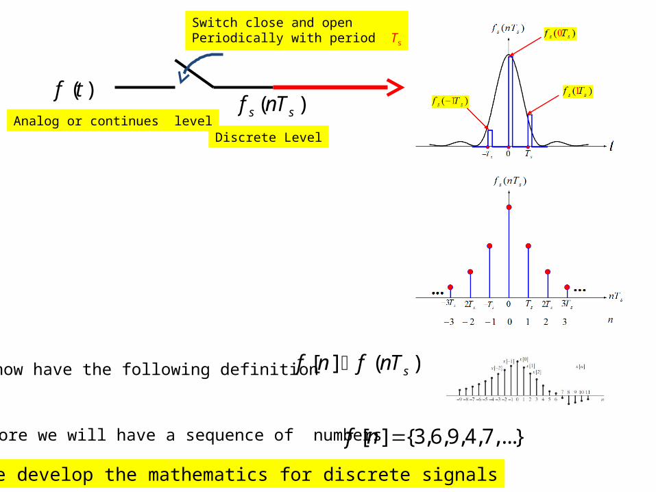
( )f t
Switch close and open Periodically with period Ts
( )s sf nT
Discrete LevelAnalog or continues level
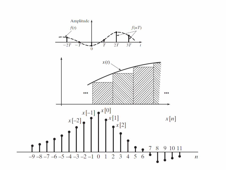
We know have the following definition [ ] ( )sf n f nT
Therefore we will have a sequence of numbers [ ] {3,6,9,4,7,...}f n
Next we develop the mathematics for discrete signals
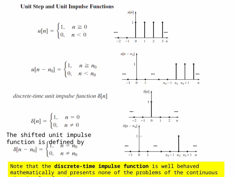
Note that the discrete-time impulse function is well behaved mathematically and presents none of the problems of the continuous time impulse function
The shifted unit impulse function is defined by
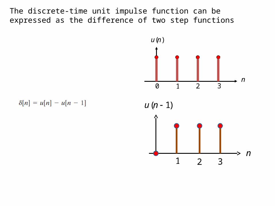
( )u n
n0 1 2 3
( 1)u n
n1 2 3
The discrete-time unit impulse function can be expressed as the difference of two step functions
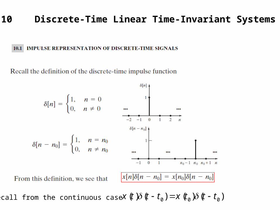
10 Discrete-Time Linear Time-Invariant Systems
0 0 0( ) ( ) ( ) ( )x t t t x t t t Recall from the continuous case
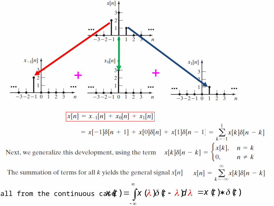
( ) ( ) ( )x t x t d
Recall from the continuous case ( ) ( )x t t
( )t ( )h t
( )t ( )h t
( ) ( )x t constant
(( ))x h t
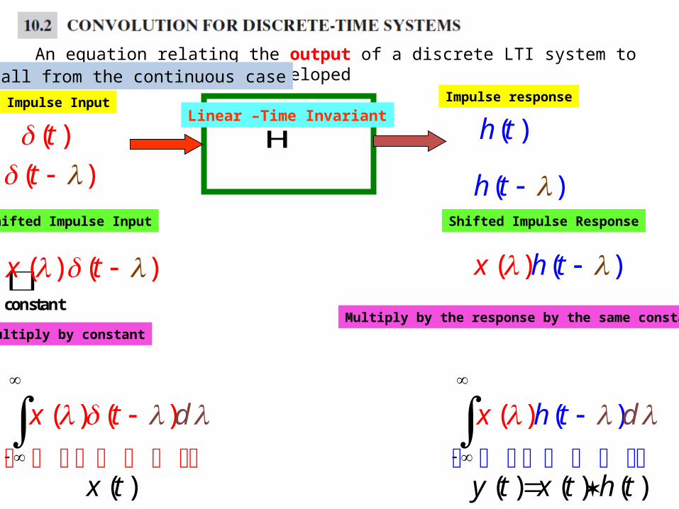
Impulse Input Impulse response
Shifted Impulse Input Shifted Impulse Response
( ) ( )x dt
HLinear –Time Invariant
)( ()x dh t
Multiply by constantMultiply by the response by the same constant
( )x t
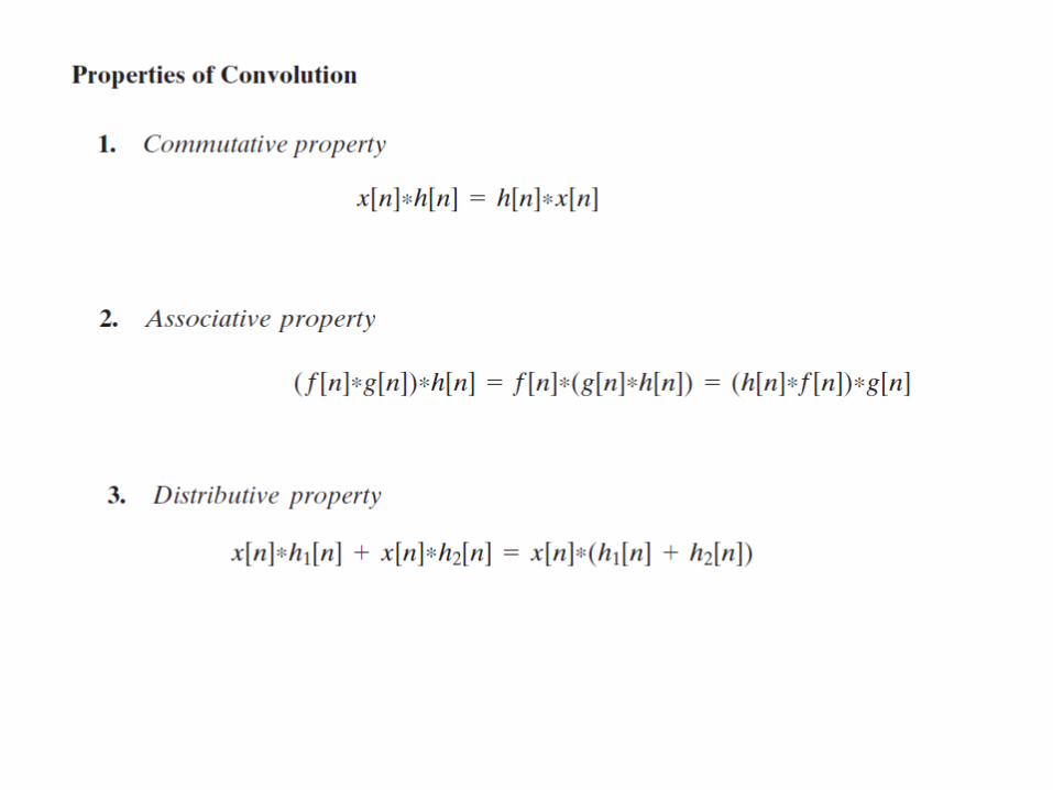
( ) ( ) ( )
y t x t h t
An equation relating the output of a discrete LTI system to its input will now be developedRecall from the continuous case
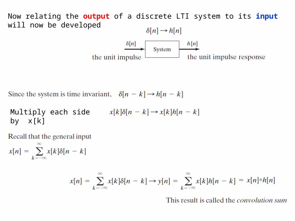
Now relating the output of a discrete LTI system to its input will now be developed
Multiply each side by x[k]
x( ) n
n
1
2 21 1
0 1 2 3 4
( ) h n
n
3
0 1 2
21
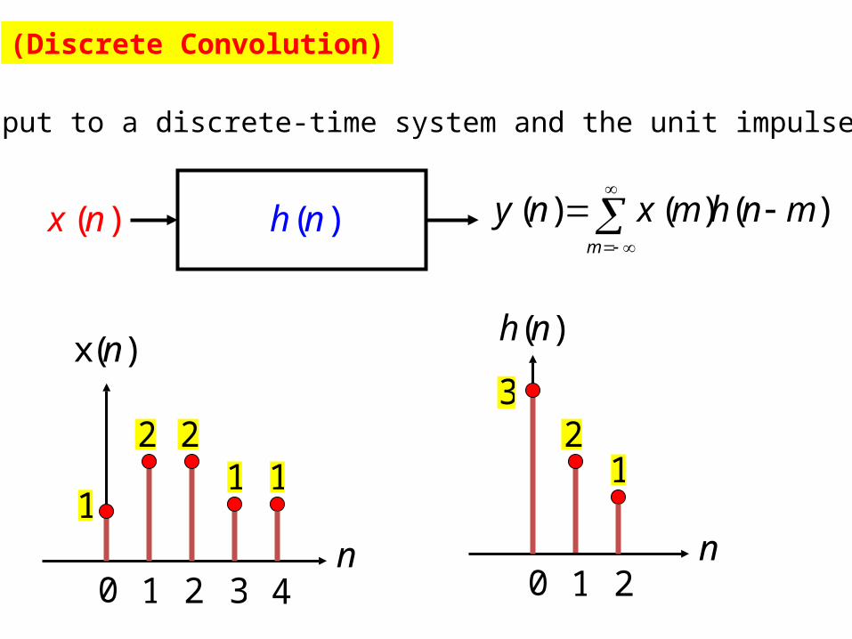
(Discrete Convolution)
Let the input to a discrete-time system and the unit impulse response
( )x n ( )h n ( ) ( ) ( )m
y n x m h n m
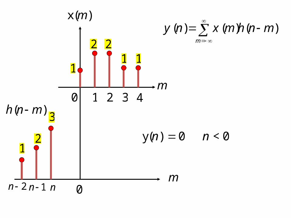
x( ) m
m
1
2 21 1
0 1 2 3 4
y( ) 0 < 0n n
( ) h n m3
21
n1n 2n 0m
( ) ( ) ( )m
y n x m h n m
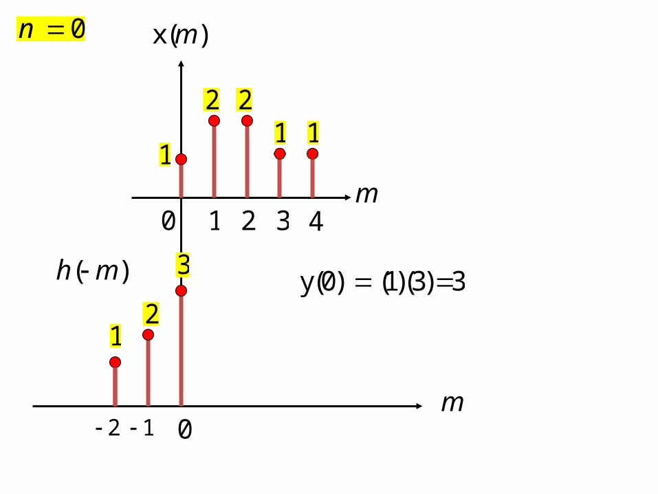
x( ) m
m
( ) h m
1
2 21 1
0 1 2 3 4
3
21
12 0m
y(0) (1)(3) 3
0n
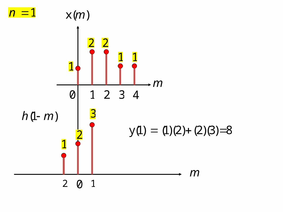
x( ) m
m
(1 ) h m
1
2 21 1
0 1 2 3 4
3
21
12 0m
y(1) (1)(2) (2)(3) 8
1n
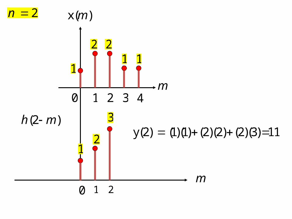
x( ) m
m
(2 ) h m
1
2 21 1
0 1 2 3 4
3
21
1 20m
y(2) (1)(1) (2)(2) (2)(3) 11
2n
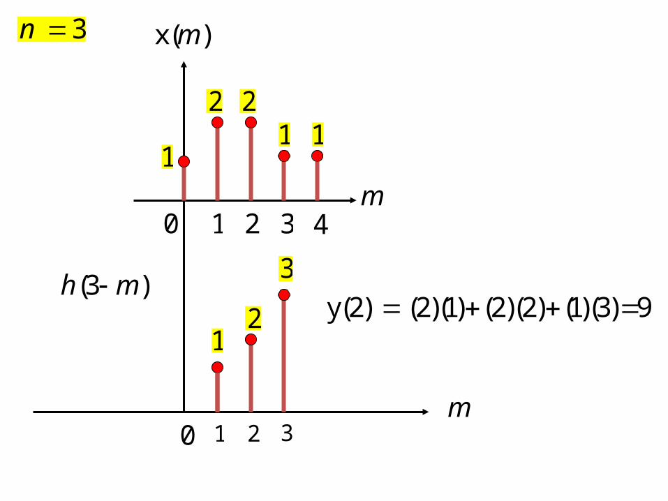
y(2) (2)(1) (2)(2) (1)(3) 9
3n x( ) m
m
(3 ) h m
1
2 21 1
0 1 2 3 4
3
21
1 20m
3
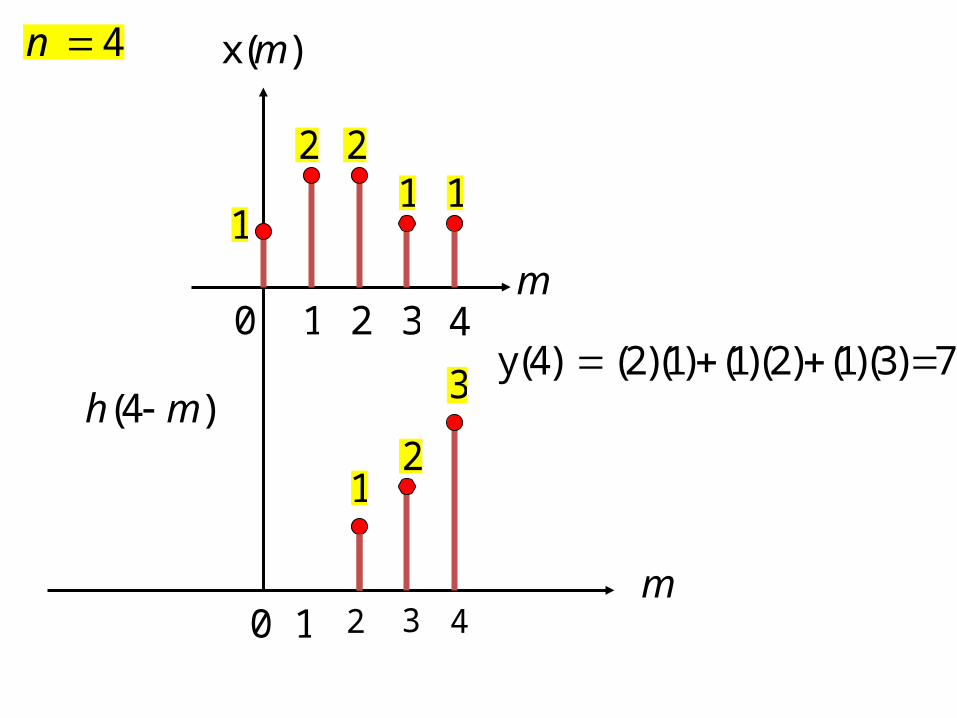
y(4) (2)(1) (1)(2) (1)(3) 7
4n x( ) m
m
(4 ) h m
1
2 21 1
0 1 2 3 4
3
21
2 30m
41
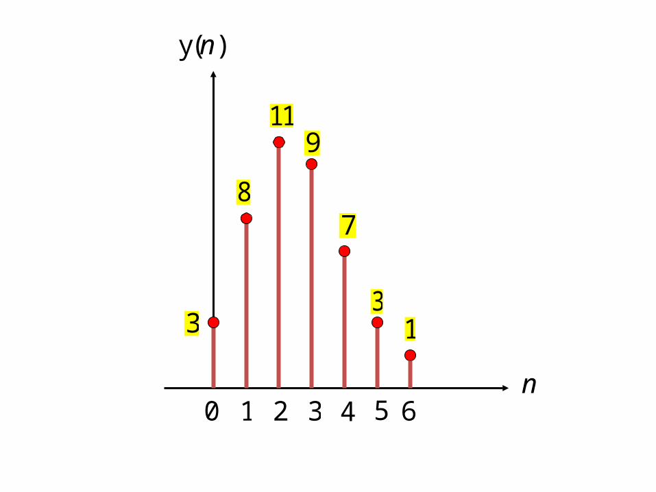
y( ) n
n
3
8
119
0 1 2 3 4
7
1
5
3
6
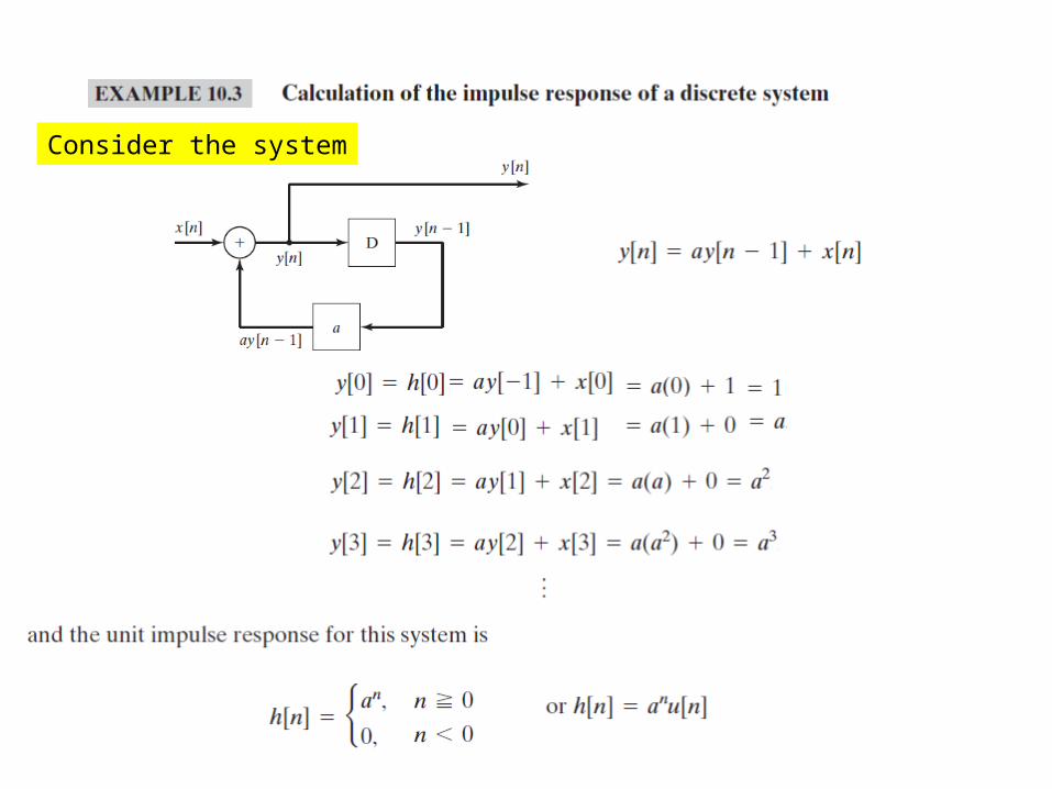
Consider the system
Recall from the continuous case
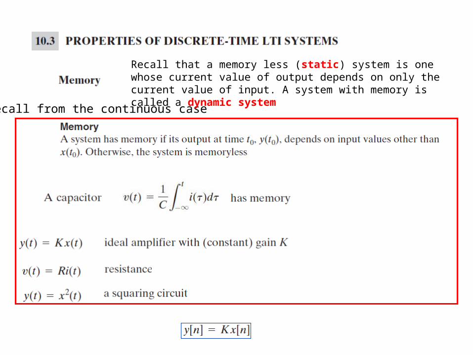
Recall that a memory less (static) system is one whose current value of output depends on only the current value of input. A system with memory is called a dynamic system
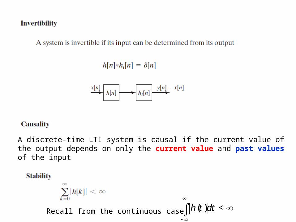
A discrete-time LTI system is causal if the current value of the output depends on only the current value and past values of the input
( ) < h t dt
Recall from the continuous case
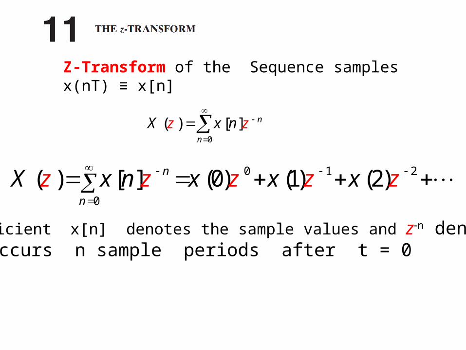
Z-Transform of the Sequence samples x(nT) ≡ x[n]
0
( ) [ ] n
n
X xz zn
0 1 2
0
( ) [ ] (0) (1) (2)n
n
X x n x xz xz z z z
The coefficient x[n] denotes the sample values and zn denote the Sample occurs n sample periods after t = 0
1 0( )
0 0
nx nT
n
( )x nT
n0 1 2 3
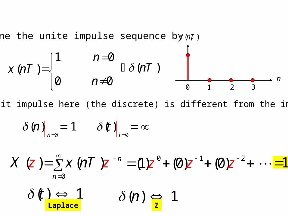
Define the unite impulse sequence by ,
( )nT
Note : the unit impulse here (the discrete) is different from the impulse (t)
0( ) 1
nn
0( )
tt
0
( ) ( ) n
n
zX T zx n
0 1 2(1) (0) (0) z z z 1
( ) 1t ( ) 1n Laplace Z
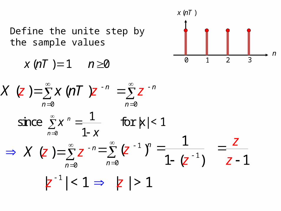
( ) 1 0x nT n
( )x nT
n0 1 2 3
0
( ) ( ) n
n
zX T zx n
0
n
n
z
0
1since for |x| < 11
n
n
xx
0
) ( n
n
z zX
1
11 ( )z
1
0
( )nn
z
1| | < 1 | | > 1 z z
1zz
Define the unite step by the sample values
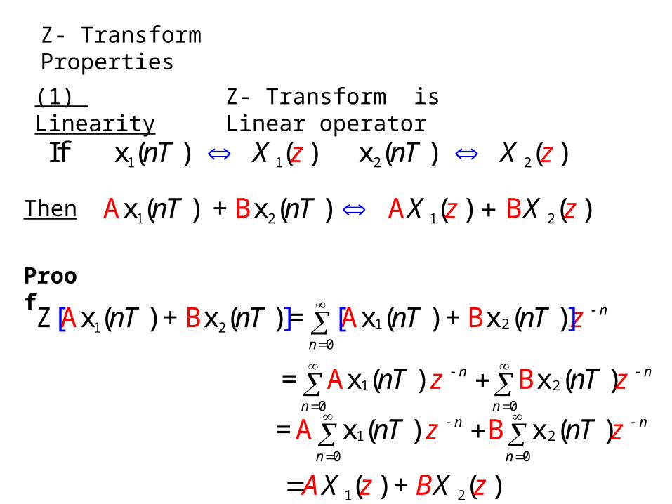
Z- Transform Properties
(1) Linearity Z- Transform is Linear operator
1 1 2 2If x ( ) ( ) x ( ) ( )znT X nT X z
Then 1 2 1 2x ( ) + x ( ) A B A ) ( )B( znT nT X X z
Proof
1 21 20
x ( ) + x (A B ) x ( ) + x (A B ) n
n
znT nT nT nT
Z[ [ ]=]
1 2
0 0
x ( ) x ( )A Bn n
n n
nT nTz z
=
1 2
0 0
x ( ) x ( )A Bn n
n n
nT nTz z
=
1 2( ) + ( )X XA z B z
0
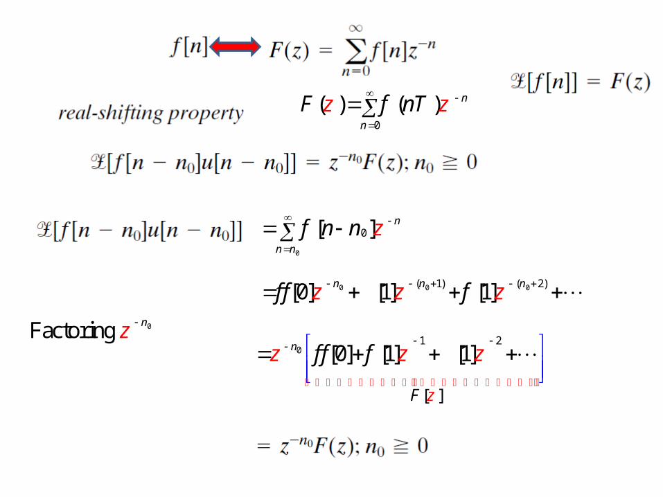
( ) ( ) n
n
zF T zf n
0 0 0( 1) ( 2)[0] [1] [1]n n nz zfzf f
0
0[ ] n
n n
zf n n
0Factorin g nz
01 2
[ ]
[0] [1] [1]n
zF
z f fzf z
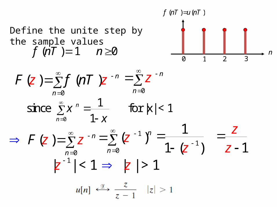
( ) 1 0f nT n
( ) ( )f nT u nT
n0 1 2 3
0
( ) ( ) n
n
zF T zf n
0
n
n
z
0
1since for |x| < 11
n
n
xx
0
) ( n
n
z zF
1
11 ( )z
1
0
( )nn
z
1| | < 1 | | > 1 z z
1zz
Define the unite step by the sample values
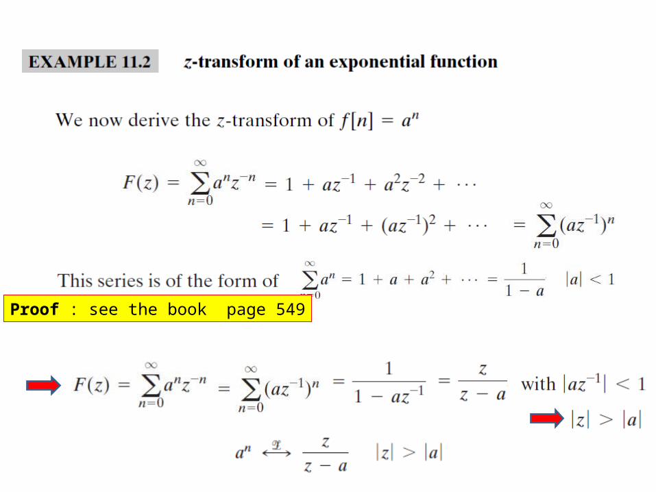
Proof : see the book page 549
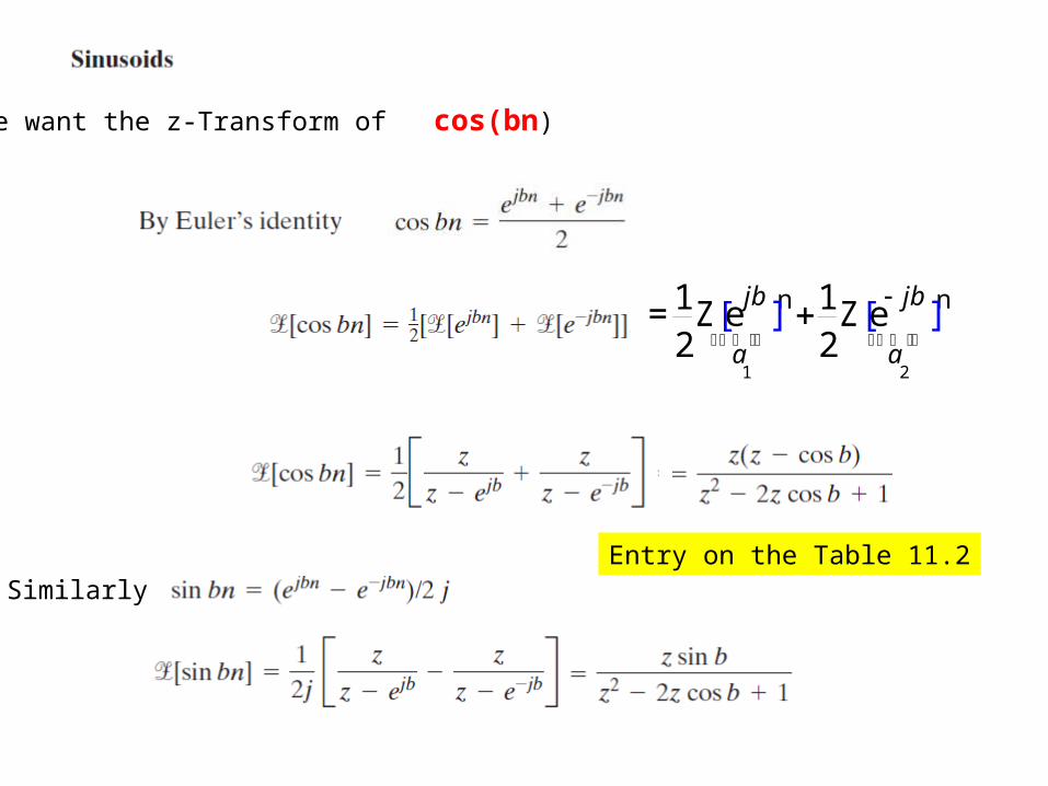
We want the z-Transform of cos(bn)
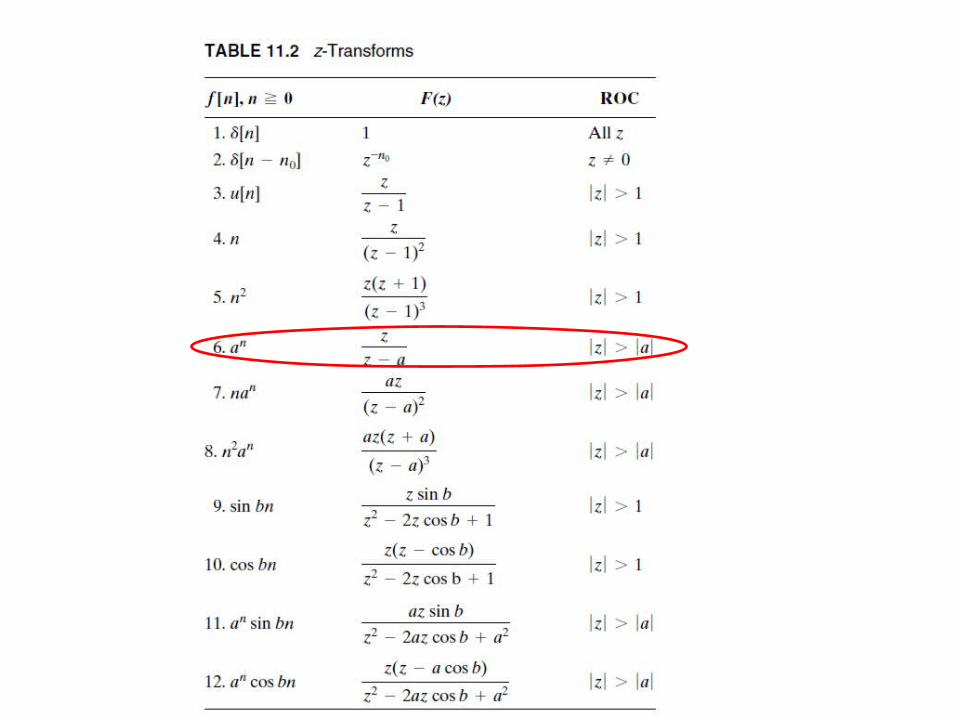
Entry on the Table 11.2Similarly
n n1 1e e2 2
jb jb [= Z[ ] ]Z
1a
2a
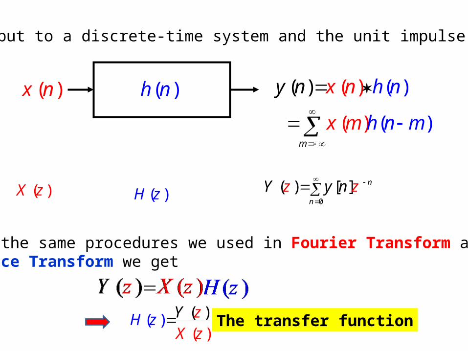
Let the input to a discrete-time system and the unit impulse response
( )x n
) )( (m
h nx m m
( )h n )( )) ((x ny n h n
( )X z0
( ) [ ] n
n
z zY y n
( )H z
Using the same procedures we used in Fourier Transform and Laplace Transform we get
(()
)(
)zH YX
zz
The transfer function
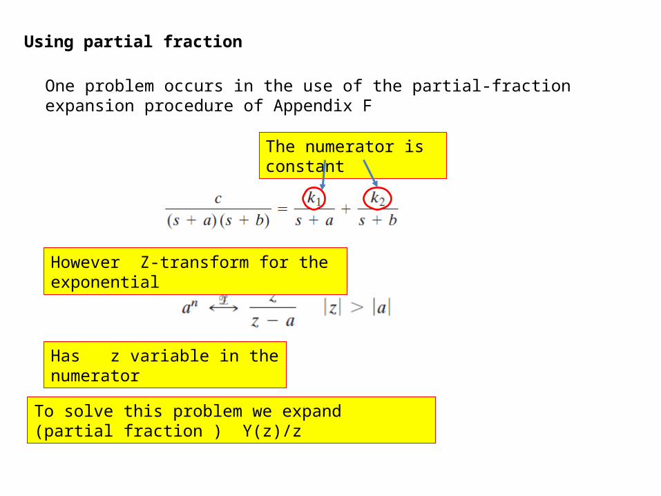
Using partial fraction
One problem occurs in the use of the partial-fraction expansion procedure of Appendix F
The numerator is constant
However Z-transform for the exponential
Has z variable in the numerator
To solve this problem we expand (partial fraction ) Y(z)/z
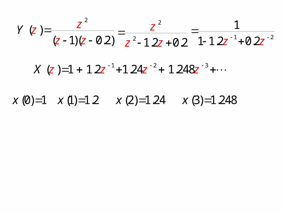
2
( )( 1)( 0.2)
zzz z
Y
2
2 1.2 0.2z
z z
1 2
11 1.2 0.2z z
1 2 3( ) 1 1.2 1.24 1.248X z z z z
(0) 1x (1) 1.2x (2) 1.24x (3) 1.248x
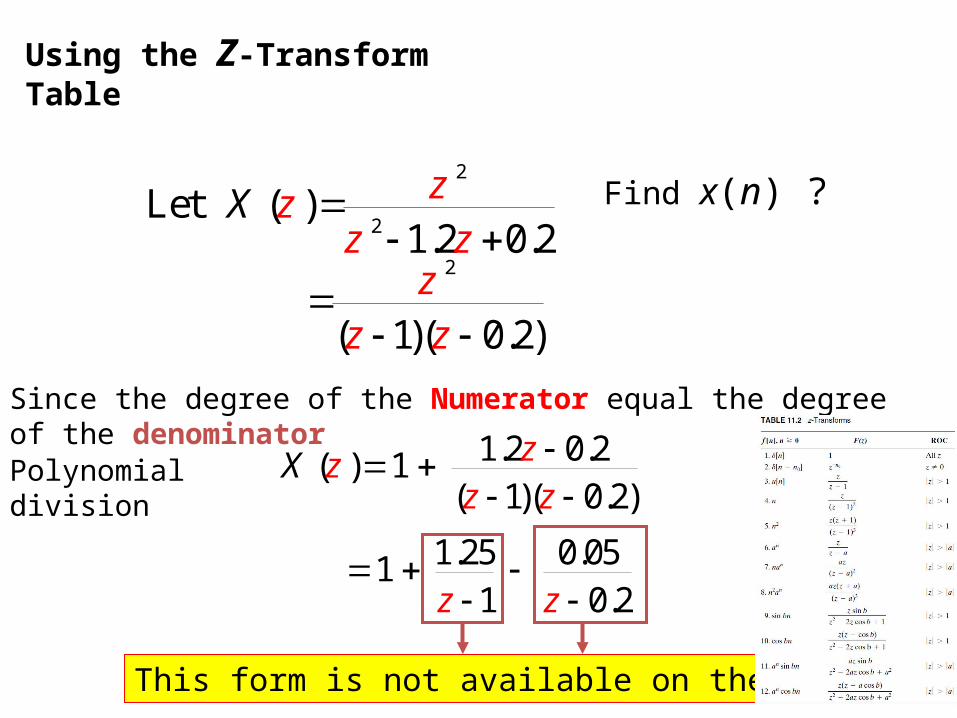
Using the Z-Transform Table
Find x(n) ?2
2Let ( )
1.2 0.2zz
z zX
Since the degree of the Numerator equal the degree of the denominator
Polynomial division
1.25 0.05 1 1 0.2z z
This form is not available on the table
2
( 1)( 0.2)z
z z
1.2 0.2( ) 1 ( 1)( 0.2)
zz
X zz
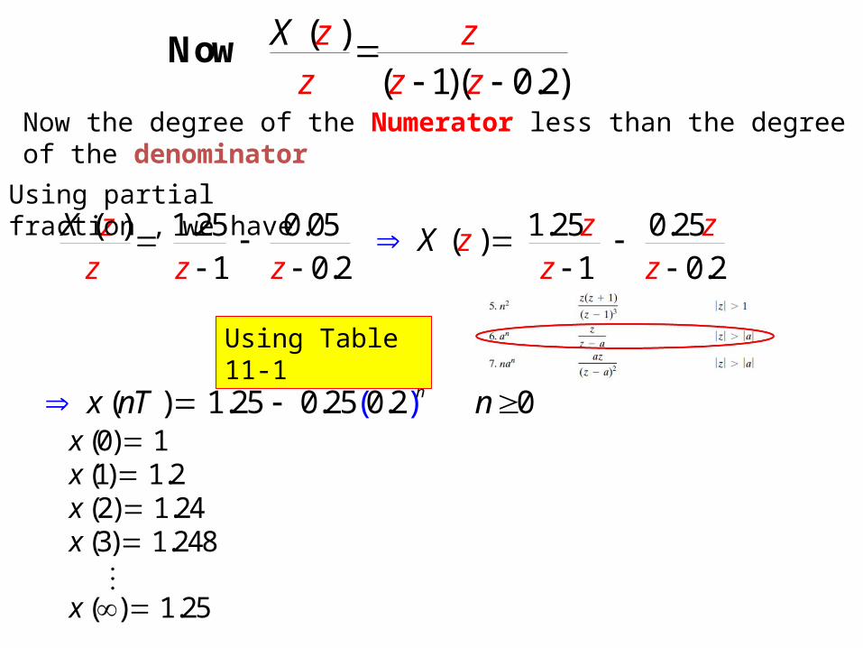
Now the degree of the Numerator less than the degree of the denominator
( ) 1.25 0.05 1 0.2
zz z
Xz
( ) ( 1)( 0.2)
z zz zX
z
Now
Using partial fraction , we have1.25 0.25 ( )
1 0.2zX zz
z z
( ) 1.25 0.25 0.2( ) 0nx nT n
Using Table 11-1
(0) 1 (1) 1.2 (2) 1.24 (3) 1.248
( ) 1.25
xxxx
x
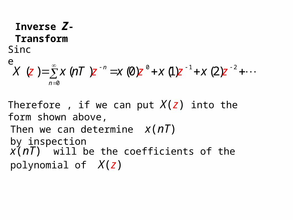
Inverse Z-Transform
0 1 2
0
( ) ( ) (0) (1) (2)n
n
X x nT x x xz z z z z
Since
Therefore , if we can put X(z) into the form shown above,
Then we can determine x(nT) by inspection
x(nT) will be the coefficients of the polynomial of X(z)
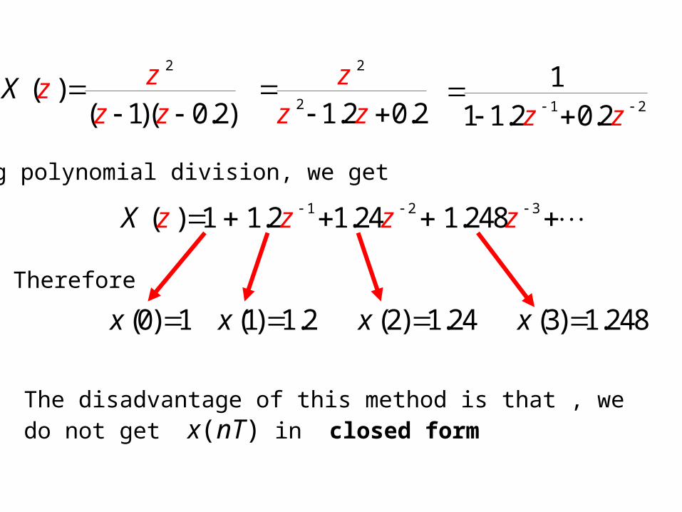
2
( )( 1)( 0.2)
zzz z
X
2
2 1.2 0.2z
z z
1 2
11 1.2 0.2z z
1 2 3( ) 1 1.2 1.24 1.248X z z z z
Using polynomial division, we get
Therefore
(0) 1x (1) 1.2x (2) 1.24x (3) 1.248x
The disadvantage of this method is that , we do not get x(nT) in closed form