Embed Size (px)
Citation preview
The Scale-Up of Oscillatory Flow Mixing
by
Keith B. Smith
Christ's College
Cambridge
September 1999
A dissertation submitted for the degree of
Doctor of Philosophy
in the University of Cambridge

To my parents
i
Summary
Oscillatory Flow Mixing is a recent development in mixing technology which has evolved
over the past decade. It has a number of similarities to other mixing technologies,
particularly pulsed and reciprocating plate columns, but at the laboratory scale has
demonstrated a number of advantageous properties. These properties (such as control of
residence time distribution, improved heat transfer and predictable mixing times) have
been demonstrated at the laboratory scale for a wide range of different potential
applications, but until now there has been a lack of firm understanding and research into
how the technology could be scaled-up into an industrial scale process.
This thesis addresses the problem of scale-up in Oscillatory Flow Mixing. It reports on a
programme of experiments on geometrically scaled apparatus with the measurement of
residence time distributions and flow visualisation as the principal methods of
investigating the wide range of flow conditions that can be achieved by control of net
flow and of oscillatory conditions. Results from these investigations are interpreted as
axial dispersion coefficients and also compared with results obtained computationally
using a fluid mechanics approach to simulate flow fields and the injection of inert tracers
into those flow fields.
Significant clarification is reported concerning the analysis of axial dispersion
measurements using the diffusion model for which conflicting solutions were identified in
the literature. The development of a flow visualisation technique using fluorescent dye
streaklines is also reported. Using the latter technique stable manifolds in Oscillatory
Flow Mixing have for the first time been experimentally observed as well as a range of
other flow regimes.
The study of scale-up was extended by the successful construction and investigation of an
alternative reactor geometry with the potential for use in large-scale plant.
From the work presented in the thesis it is concluded that Oscillatory Flow Mixing is a
technology which in general lends itself readily to scaling-up from laboratory to pilot
plant scale, and most probably to industrial scale. Experiments performed on small
laboratory apparatus (containing less than one litre of fluid) can with confidence be used
to predict mixing behaviour in much larger plant (containing hundreds of litres of fluid.)
ii
Preface
The work described in this dissertation was carried out in the University of Cambridge
Department of Chemical Engineering between October 1995 and September 1999. It is
my original work, unless it is acknowledged to be otherwise in the text, and includes
nothing which is the outcome of work done in collaboration. Neither the present
dissertation, nor any part thereof, has been previously submitted for a degree at any
university.
I am indebted to my supervisor and mentor Dr Malcolm Mackley for his help and
enthusiasm throughout the course of this research. I would also like to thank the many
departmental staff who have given practical assistance and valuable discussions towards
the project, and to thank especially Rob Marshall for his technical support.
I am most grateful to the E.P.S.R.C. for providing funds for the research.
Keith B. Smith
Christ's College
Cambridge
September 1999
iii
1. Introduction
1.1 Motivation for the Study 1:1
1.2 The Problem of Scale-up 1:2
1.3 Structure of the Thesis 1:3
2. Background
2.1 Background to O.F.M. 2:1
2.1.1 A General Description of O.F.M.
2.1.2 Dimensionless Groups Used to Describe O.F.M.
2.1.3 An Overview of Research into O.F.M.
2.1.4 Experimental Studies of Axial Dispersion in O.F.M.
2.1.5 Numerical Simulation Studies of O.F.M.
2.2. Measurement and Modelling of Axial Dispersion 2:13
2.2.1 Models Available for the Quantification of Axial Dispersion
2.2.2 Solutions to the Diffusion Equation for the Imperfect Pulse Technique
2.2.3 Estimates of Axial Dispersion from Fluid Mechanical Simulations
2.3 Studies of Systems Analogous to O.F.M. 2:19
2.3.1 Pulsed Packed Beds
2.3.2 Reciprocating Plate Columns
3. Apparatus and Experimental Method
3.1 Design Criteria and Construction of Apparatus 3:1
3.1.1 The Required Range of Operating Conditions for the Apparatus
3.1.2 Construction of the Apparatus
3.2 Experimental Methods 3:11
3.2.1 Imperfect Pulse Dye Tracer Experiments
3.2.2 Flow Visualisation Using Fluorescent Dye Streaklines
4. Analysis of Results for Axial Dispersion
4.1 Development of Axial Dispersion Analysis Programme in Matlab 4:1
4.2 Debugging of the Imperfect Pulse Solution to the Diffusion Equation 4:6
4.3 Case Study 1 - Analysis of a Typical Imperfect Pulse Tracer Experiment 4:10
4.4 Case Study 2 - Analysis of a Typical Tracer Experiment with No Net Flow 4:13
iv
5. Results of Experimental Axial Dispersion Measurements
5.1 Oscillation with Net Flow – 24 mm, 54 mm and 150 mm Apparatus 5:1
5.2 Oscillation with No Net Flow – 24 mm, 54 mm and 150 mm Apparatus 5:7
5.3 Net Flow with No Oscillation – 24 mm, 54 mm and 150 mm Apparatus 5:12
5.4 Study of Backmixing for O.F.M. with Net Flow 5:13
5.5 Correlation for Axial Dispersion at High Reynolds Numbers 5:15
6. Axial Dispersion Measurements from Fluid Mechanical Simulation
6.1 Simulation of Axial Dispersion in O.F.M. Using Fluid Marker Particles 6:1
6.2 Results for Simulation of Axial Dispersion in O.F.M. 6:6
7. Flow Visualisations Obtained by Experiment and by Simulation
7.1 Flow Visualisation - Net Flow with No Oscillation 7:2
7.2 Flow Visualisation - Oscillation with No Net Flow 7:8
7.3 Flow Visualisation - Oscillation with Net Flow 7:15
8. Multi-Orifice Baffles
8.1 Concept and Design 8:1
8.2 Experimental Programme 8:3
8.3 Axial Dispersion Results and Analysis 8:6
8.4 Flow Visualisation 8:8
8.5 Estimates of Radial Dispersion 8:18
9. Discussion
9.1 Relating Axial Dispersion Measurements to Flow Visualisation 9:1
9.2 Comparison of Results with Those in the Literature 9:4
9.3 Multi-Orifice Baffles as a Route to Scale-Up 9:7
9.4 Heat Transfer 9:9
9.5 Energy Dissipation 9:10
9.6 Engineering Considerations for Large Scale O.F.M. 9:11
10. Conclusions and Suggestions for Further Work
10.1 Conclusions 10:1
10.2 Suggestions for Further Work 10:3

v
References
Appendices:
I Hydraulic Sizing Calculations and Circuit Diagram
II Electronic Servo-Control Circuits
III Optical Dye Tracer Technique
IV Matlab Analysis Programme for Axial Dispersion
V Treatment of Errors
VI Fluid Mechanical Simulation
Nomenclature
1:1
1. Introduction
1.1 Motivation for the Study
It has often been the goal of chemical engineers to construct a reactor design which would
give perfect plug flow, even under variable throughput conditions. Tubular reactors are a
close approximation, yet in general are reliant on turbulent flow, are susceptible to
variations in throughput and can for long residence times require very long tubes with
resulting high pressure differences along the length of the reactor.
Oscillatory Flow Mixing (O.F.M.) is a recent development in mixing technology which
has been researched over the past decade. It has a number of similarities to other tubular
mixing technologies, particularly pulsed and reciprocating plate columns, but at the
laboratory scale has demonstrated a number of advantageous properties (Mackley 1987
and Mackley 1991). Most notably, control of the oscillatory conditions when operating
as a continuous process allows axial dispersion to be minimised (Dickens et al 1989),
permitting the control of residence time distributions independently of the throughput rate
(Mackley & Ni 1991). In this way the technology can be operated as a near-perfect plug
flow device, unaffected by changes in throughput.
O.F.M. generally consists of periodically spaced annular baffles inside a long tube in
which either a liquid or a multiphase mixture is oscillated axially (Brunold et al 1989).
This flow past the baffles induces vortices which provide both axial and radial mixing in
the tube. The intensity of mixing can be varied by tuning the oscillatory conditions
(amplitude and frequency of oscillation) and several different mixing regimes have been
identified, ranging from creeping laminar to fully turbulent flow (Howes 1988).
The ability to generate radial mixing gives a unique form of control in respect of intensity
of mixing, axial dispersion and other transfer processes. These and other properties have
been studied on a number of occasions by previous researchers, both by experiment and
simulation, but such studies have in general been limited to laboratory scale with at most
only a few litres of liquid in the reactor volume. There is therefore a need to understand
more fully the effect of scale-up on the performance of Oscillatory Flow Mixing.
1:2
1.2 The Problem of Scale-up
Scale-up has traditionally been a problem for technologies such as the Stirred Tank
Reactor (S.T.R.) or Continuous Stirred Tank Reactor (C.S.T.R.) where mixing is a very
strong function of scale: laboratory scale experiments cannot reliably predict behaviour
of large scale plant, where stagnant zones and excessive shear-rates at the impeller tip can
limit the effectiveness of the reactor (Perry 1984 Chapter 4). In this case, the expensive
and time-consuming construction of pilot scale plant is necessary before design of the
full-scale process.
Until now there has been a lack of firm understanding and research into how O.F.M.
technology could be scaled-up into an industrial scale process. Individual properties such
as control of residence time distribution, improved heat transfer (Mackley & Stonestreet
1995) and particle suspension (Mackley et al 1993) have been demonstrated at the
laboratory scale, but the issue of scale-up not addressed.
By the nature and design of O.F.M. it has always been hoped that predictions of large-
scale behaviour would be reliable, but problems have existed in that, according to the
expected scaling laws, mixing-rate would decrease rapidly (inverse square law) as a
function of increasing tube diameter. Different schemes have been proposed to
circumvent this problem, including arrangements with many smaller tubes bundled in
parallel (Mackley & Ni 1993) or one large diameter tube containing baffles with multiple
orifices (this thesis).
1.3 Structure of the Thesis
The thesis studies the effects of scale-up on O.F.M.. In order to characterize the effects,
axial dispersion has been chosen as the principal parameter to be measured as a function
of tube diameter. Knowledge of axial dispersion allows for the prediction of bulk mixing
times (batch systems) or of residence time distributions (continuous systems.) Flow
visualisation is also used to compare flow conditions for experiments under different
conditions, as well as for experiments under dynamically similar conditions with varying
tube diameter. Both experiment and simulation are used to research these properties.
Following this introduction, the thesis commences in Chapter 2 with a survey of the
background literature relevant to the scale-up of O.F.M., measurement and quantification
of axial dispersion, and flow visualisation. The background to analogous systems such as
1:3
pulsed packed beds and reciprocating plate columns is also discussed in so far as it is
relevant to O.F.M..
Chapter 3 introduces the sets of experimental apparatus that have been designed and
constructed in order to investigate axial dispersion and scale-up. There are three sets of
geometrically similar apparatus with tube diameters 24, 54 and 150 mm. The reasons for
choice of construction and selection of oscillation device are discussed, as well as the
selection and development of an imperfect pulse dye-tracer technique to measure axial
dispersion. Brief details of the technique developed for flow visualisation are also
discussed.
In Chapter 4 the development of software for the analysis of axial dispersion using the
diffusion model is described. During the development of the software it was discovered
that solutions to the diffusion equation quoted in the literature were inconsistent, and the
correct solution for the given boundary conditions was identified. Using data gathered
during a typical experiment, a case study analysis is then presented to show how a value
for the axial dispersion coefficient is arrived at for a given set of experimental conditions.
Chapters 5 and 6 present the results of axial dispersion coefficients obtained by
experiment and by fluid mechanical simulation respectively. Experiments were
performed on the 24, 54 and 150 mm diameter sets of apparatus. The fluid mechanical
simulation is derived from a Fortran code written by co-workers in the Department of
Chemical Engineering, Cambridge University (detailed in Appendix VI) and run on a Sun
Workstation. For the purposes of this thesis it has been adapted to simulate experimental
dye tracer experiments.
Flow visualisation of fluid streaklines captured experimentally using video and still
photography are compared in Chapter 7 with flow fields obtained by fluid mechanical
simulation. Different flow regimes are identified and the effect of tube diameter on the
transition between flow regimes is discussed.
In light of the results presented in Chapters 5 to 7, in Chapter 8 a potential design for
large-scale O.F.M. is investigated in the 150 mm diameter apparatus, using closely spaced
baffles with 37 orifices per baffle in place of the conventional single-orifice baffles with a
wide spacing. Estimates of axial and radial dispersion are given, together with flow
visualisation. The work highlights the observation (both experimentally and by
simulation) of manifolds in the flow field under certain low Reynolds Number oscillatory
conditions.
1:4
An important aspect of the thesis is the relating of the measured trends in axial dispersion
to the appearance of the physical flow, whether laminar, chaotic or turbulent. This is
presented in Chapter 9, which then continues to discuss the relationship between the new
results presented in this thesis and those already in the literature. Consideration is also
given to the likely effect of scale-up on heat transfer and energy dissipation. Finally, brief
notes are given concerning likely engineering considerations when designing a large-scale
O.F.M. plant.
The main part of the thesis is concluded in Chapter 10 followed by a list of references and
nomenclature; appendices on the apparatus design, Optical Dye Tracer Technique, Fluid
Mechanical Simulation and Treatment of Errors are given at the end.
2:1
2. Background
This chapter surveys the background literature which is relevant to the scale-up of
Oscillatory Flow Mixing (O.F.M.), and is divided into three sections:
§2.1 presents a basic description of O.F.M. and a summary of the range of direct research
into the various properties of O.F.M. from which industrial interest in the technology has
arisen. Then follows a chronology and description of the results and conclusions drawn
from the various published O.F.M. experimental and modelling studies most relevant to
this thesis (concerning the measurement and quantification of axial dispersion, and flow
visualisation).
§2.2 deals in more detail with the measurement and modelling of axial dispersion. It
presents the literature available on experimental techniques of axial dispersion
measurement and on the models that have been used to quantify axial dispersion.
Emphasis is placed upon the diffusion model (the model adopted in this thesis) for which
it is shown that the literature presents conflicting conclusions. Reported methods for
theoretical measurements of axial dispersion using fluid mechanical simulations are also
presented.
In §2.3 the background to analogous systems such as reciprocating plate columns is
discussed in so far as it is relevant to O.F.M., particularly in respect of scale-up.
2.1 Background to O.F.M.
This section is divided into four parts:
§2.1.1 gives a generalised description of O.F.M.. §2.1.2 presents the principal
dimensionless groups used in the literature to describe the fluid flow in O.F.M.. §2.1.3
presents a tabular summary of the main reported experimental research into O.F.M. and
shows also the range of tube size, baffle geometry, oscillation method and oscillatory
conditions studied. §2.1.4 gives an overview of the results drawn from experimental
studies of O.F.M. with emphasis on axial dispersion and flow visualisation. §2.1.5
discusses numerical simulation studies of O.F.M..
2.1.1 A General Description of O.F.M.
Oscillatory Flow Mixing is generally understood to be a long tube of typically between 12
mm and 150 mm diameter containing periodically spaced baffles and in which a liquid or
2:2
multiphase fluid is oscillated axially by means of diaphragms, bellows or pistons at one or
both ends of the tube. The resulting flow of fluid past the baffles induces vortex
formation and hence radial mixing from which the various useful properties of O.F.M.
stem. For small amplitude, low frequency oscillations the flow is viscous and well
defined; for large amplitude, high frequency oscillations the flow is chaotic or even
turbulent.
A number of different configurations for the baffles have been tested including central
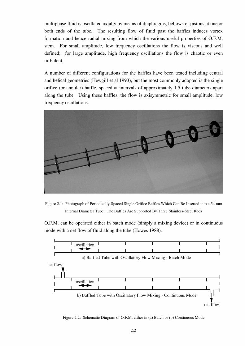
and helical geometries (Hewgill et al 1993), but the most commonly adopted is the single
orifice (or annular) baffle, spaced at intervals of approximately 1.5 tube diameters apart
along the tube. Using these baffles, the flow is axisymmetric for small amplitude, low
frequency oscillations.
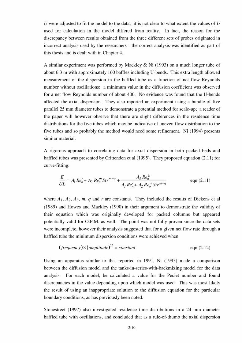
Figure 2.1: Photograph of Periodically-Spaced Single Orifice Baffles Which Can Be Inserted into a 54 mm
Internal Diameter Tube. The Baffles Are Supported By Three Stainless-Steel Rods
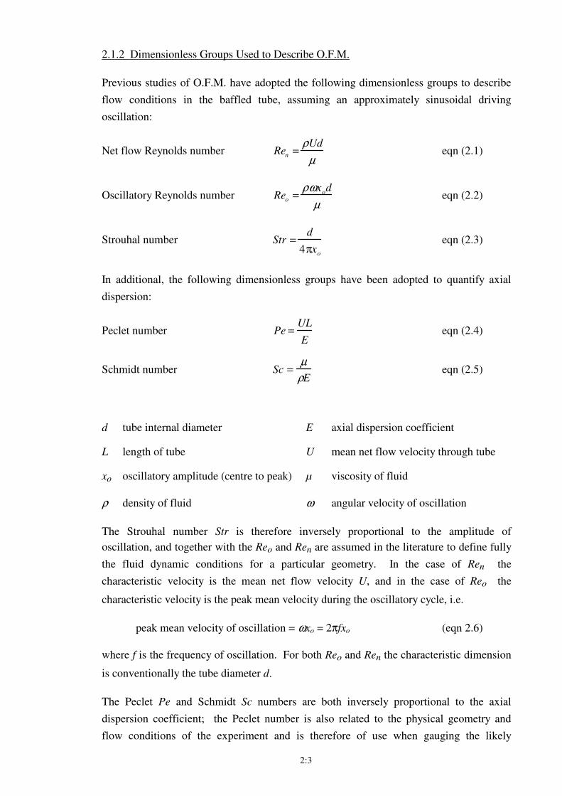
O.F.M. can be operated either in batch mode (simply a mixing device) or in continuous
mode with a net flow of fluid along the tube (Howes 1988).
oscillation
a) Baffled Tube with Oscillatory Flow Mixing - Batch Mode
oscillation
net flow
b) Baffled Tube with Oscillatory Flow Mixing - Continuous Mode
net flow
Figure 2.2: Schematic Diagram of O.F.M. either in (a) Batch or (b) Continuous Mode
2:3
2.1.2 Dimensionless Groups Used to Describe O.F.M.
Previous studies of O.F.M. have adopted the following dimensionless groups to describe
flow conditions in the baffled tube, assuming an approximately sinusoidal driving
oscillation:
Net flow Reynolds number Ren =ρUd
µ eqn (2.1)
Oscillatory Reynolds number Reo =ρωxod
µ eqn (2.2)
Strouhal number Str =d
4πxo
eqn (2.3)
In additional, the following dimensionless groups have been adopted to quantify axial
dispersion:
Peclet number Pe =UL
E eqn (2.4)
Schmidt number Sc =µ
ρE eqn (2.5)
d tube internal diameter E axial dispersion coefficient
L length of tube U mean net flow velocity through tube
xo oscillatory amplitude (centre to peak) µ viscosity of fluid
ρ density of fluid ω angular velocity of oscillation
The Strouhal number Str is therefore inversely proportional to the amplitude of
oscillation, and together with the Reo and Ren are assumed in the literature to define fully
the fluid dynamic conditions for a particular geometry. In the case of Ren the
characteristic velocity is the mean net flow velocity U, and in the case of Reo the
characteristic velocity is the peak mean velocity during the oscillatory cycle, i.e.
peak mean velocity of oscillation = ωxo = 2πfxo (eqn 2.6)
where f is the frequency of oscillation. For both Reo and Ren the characteristic dimension
is conventionally the tube diameter d.
The Peclet Pe and Schmidt Sc numbers are both inversely proportional to the axial
dispersion coefficient; the Peclet number is also related to the physical geometry and
flow conditions of the experiment and is therefore of use when gauging the likely
2:4
magnitude of experimental errors or the effectiveness of a particular reactor, whereas the
Schmidt number is related to the fundamental properties of the fluid and therefore is
relevant for the consideration of scale-up.
An obvious limitation of the dimensionless groups adopted in the literature (equations 2.1
to 2.6) is that they do not take into account the spacing of the baffles, the baffle thickness
nor the orifice diameter. Although all these geometrical parameters have been shown to
have an effect on the fluid mechanics in O.F.M. (Brunold et al 1989, Kim & Baird 1976b,
Saraiva 1997), this thesis effectively deals only with one geometry for single-orifice
baffles and it is therefore not helpful to include the baffle geometry in the dimensionless
groups for the presentation of data.
A further subject for debate is the value of the characteristic velocity used to calculate Reo
. It might be supposed that the strong effect of orifice diameter on the generation of
vortices (for a given mean oscillatory flow) should be taken into account; again, because
only a single orifice diameter was investigated in this thesis it is not helpful to include this
geometrical factor in the dimensionless groups, as well as wishing to maintain a
consistent nomenclature with other research in the area of O.F.M..
The definition of the Strouhal number as applied to O.F.M. was discussed by Ni & Gough
(1997) who concluded that since the Strouhal number was originally conceived to
describe the frequency of vortex shedding around objects in a flow (for example vortex
shedding behind a cylinder in a flowing fluid) then a more consistent definition of the
Strouhal number would be
Modified Strouhal number (Ni & Gough 1997) Str =c
πxo
eqn (2.7)
where c is the orifice diameter. This modified definition of the Strouhal number takes
into account not only that the orifice diameter (rather than tube diameter) is the more
appropriate length scale but also that two vortices are shed (one on each side of the baffle)
during each full oscillation. The modified definition appears to be well conceived,
however the experiments in this thesis do not vary orifice diameter therefore in order to
make consistent comparisons with other research, the more widely defined version of the
Strouhal number (eqn 2.3) will be used for the presentation of data.
2:5
2.1.3 An Overview of Research into O.F.M.
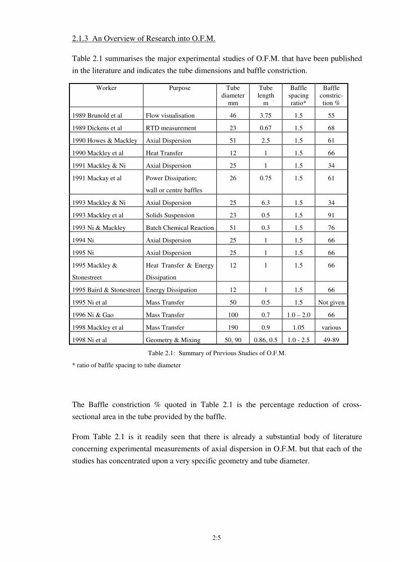
Table 2.1 summarises the major experimental studies of O.F.M. that have been published
in the literature and indicates the tube dimensions and baffle constriction.
Worker Purpose Tube diameter
mm
Tube length
m
Baffle spacing ratio*
Baffle constric-tion %
1989 Brunold et al Flow visualisation 46 3.75 1.5 55
1989 Dickens et al RTD measurement 23 0.67 1.5 68
1990 Howes & Mackley Axial Dispersion 51 2.5 1.5 61
1990 Mackley et al Heat Transfer 12 1 1.5 66
1991 Mackley & Ni Axial Dispersion 25 1 1.5 34
1991 Mackay et al Power Dissipation;
wall or centre baffles
26 0.75 1.5 61
1993 Mackley & Ni Axial Dispersion 25 6.3 1.5 34
1993 Mackley et al Solids Suspension 23 0.5 1.5 91
1993 Ni & Mackley Batch Chemical Reaction 51 0.3 1.5 76
1994 Ni Axial Dispersion 25 1 1.5 66
1995 Ni Axial Dispersion 25 1 1.5 66
1995 Mackley &
Stonestreet
Heat Transfer & Energy
Dissipation
12 1 1.5 66
1995 Baird & Stonestreet Energy Dissipation 12 1 1.5 66
1995 Ni et al Mass Transfer 50 0.5 1.5 Not given
1996 Ni & Gao Mass Transfer 100 0.7 1.0 – 2.0 66
1998 Mackley et al Mass Transfer 190 0.9 1.05 various
1998 Ni et al Geometry & Mixing 50, 90 0.86, 0.5 1.0 - 2.5 49-89
Table 2.1: Summary of Previous Studies of O.F.M.
* ratio of baffle spacing to tube diameter
The Baffle constriction % quoted in Table 2.1 is the percentage reduction of cross-
sectional area in the tube provided by the baffle.
From Table 2.1 is it readily seen that there is already a substantial body of literature
concerning experimental measurements of axial dispersion in O.F.M. but that each of the
studies has concentrated upon a very specific geometry and tube diameter.
2:6
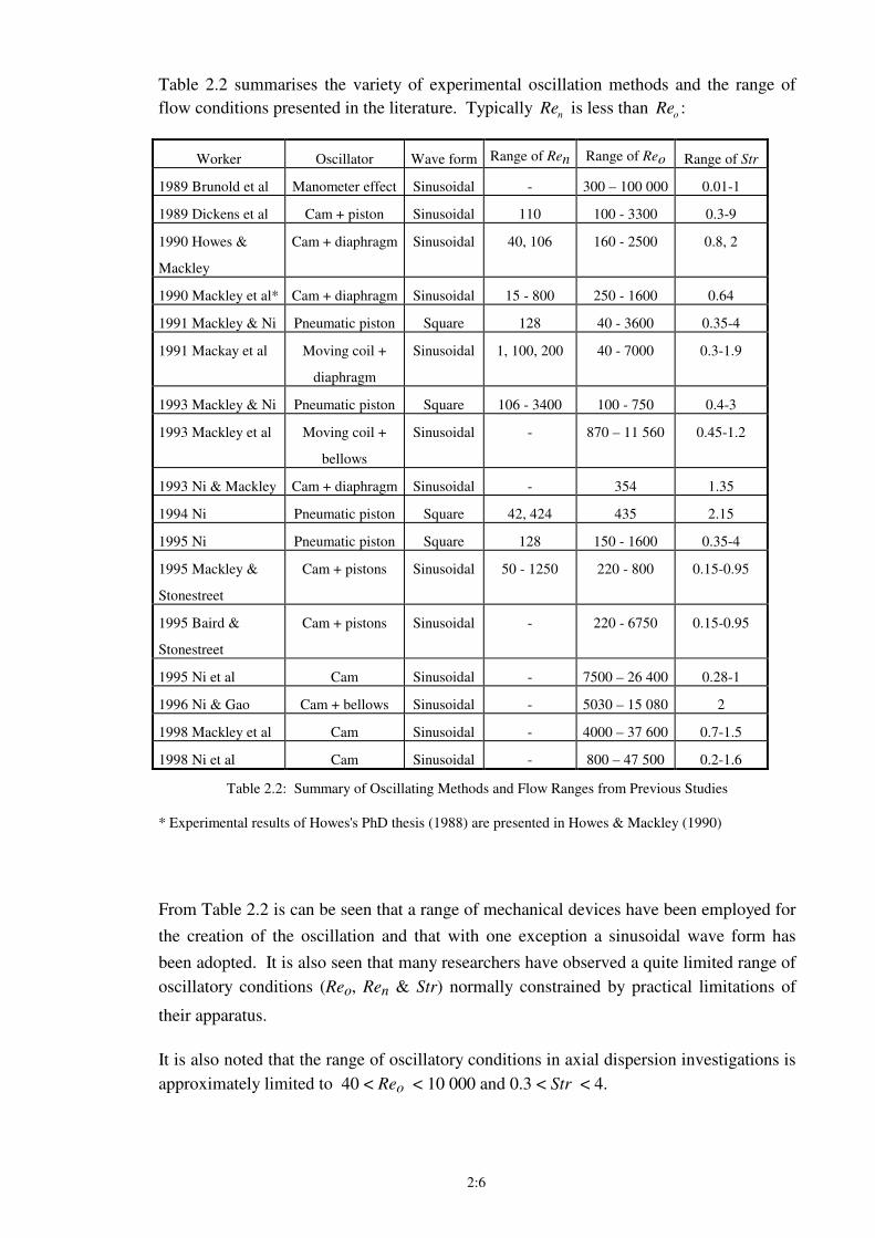
Table 2.2 summarises the variety of experimental oscillation methods and the range of
flow conditions presented in the literature. Typically Ren is less than Reo :
Worker Oscillator Wave form Range of Ren Range of Reo Range of Str
1989 Brunold et al Manometer effect Sinusoidal - 300 – 100 000 0.01-1
1989 Dickens et al Cam + piston Sinusoidal 110 100 - 3300 0.3-9
1990 Howes &
Mackley
Cam + diaphragm Sinusoidal 40, 106 160 - 2500 0.8, 2
1990 Mackley et al* Cam + diaphragm Sinusoidal 15 - 800 250 - 1600 0.64
1991 Mackley & Ni Pneumatic piston Square 128 40 - 3600 0.35-4
1991 Mackay et al Moving coil +
diaphragm
Sinusoidal 1, 100, 200 40 - 7000 0.3-1.9
1993 Mackley & Ni Pneumatic piston Square 106 - 3400 100 - 750 0.4-3
1993 Mackley et al Moving coil +
bellows
Sinusoidal - 870 – 11 560 0.45-1.2
1993 Ni & Mackley Cam + diaphragm Sinusoidal - 354 1.35
1994 Ni Pneumatic piston Square 42, 424 435 2.15
1995 Ni Pneumatic piston Square 128 150 - 1600 0.35-4
1995 Mackley &
Stonestreet
Cam + pistons Sinusoidal 50 - 1250 220 - 800 0.15-0.95
1995 Baird &
Stonestreet
Cam + pistons Sinusoidal - 220 - 6750 0.15-0.95
1995 Ni et al Cam Sinusoidal - 7500 – 26 400 0.28-1
1996 Ni & Gao Cam + bellows Sinusoidal - 5030 – 15 080 2
1998 Mackley et al Cam Sinusoidal - 4000 – 37 600 0.7-1.5
1998 Ni et al Cam Sinusoidal - 800 – 47 500 0.2-1.6
Table 2.2: Summary of Oscillating Methods and Flow Ranges from Previous Studies
* Experimental results of Howes's PhD thesis (1988) are presented in Howes & Mackley (1990)
From Table 2.2 is can be seen that a range of mechanical devices have been employed for
the creation of the oscillation and that with one exception a sinusoidal wave form has
been adopted. It is also seen that many researchers have observed a quite limited range of
oscillatory conditions (Reo, Ren & Str) normally constrained by practical limitations of
their apparatus.
It is also noted that the range of oscillatory conditions in axial dispersion investigations is
approximately limited to 40 < Reo < 10 000 and 0.3 < Str < 4.
2:7
2.1.4 Experimental Studies of Axial Dispersion in O.F.M.
The earliest observation of O.F.M. was as part of a 4th year research project in the early
1980s under the supervision of Dr M.R. Mackley at the Department of Chemical
Engineering, Cambridge University and which was later published as Brunold et al
(1989). Using a manometer-style 46 mm diameter tube containing annular baffles they
observed the flow over a large range of amplitudes created by unforced simple harmonic
oscillation of the fluid following an initial height displacement on one side of the U-
shaped tube. They estimated viscous and eddy dissipation energy losses in the flow by
measuring damping. They used a baffle constriction of 55% and observed flows with a
baffle spacing equal to 1, 1.5 and 2 tube diameters; they demonstrated that 1.5 tube
diameters was a good compromise between excessive channelling of the flow (1 tube
diameter spacing) and insufficient vortex interaction (2 tube diameters spacing). This
baffle spacing has been chosen by many subsequent researchers but was not necessarily
optimised since subsequent studies have involved smaller amplitude oscillations together
with varying baffle constriction. They were able to observe the flow using neutrally
buoyant 100 µm polyethylene particles seeded into the flow and illuminated by a slit light
source in a cross-section through the flow.
In a subsequent 4th year research project in 1984 Dickens and Williams measured
residence time distributions in a 23 mm diameter baffled tube with an oscillatory flow
superimposed upon a net flow. Their findings were subsequently published as Dickens et
al (1989). They injected a potassium chloride solution (KCl) tracer into the baffled tube
inflow and placed a conductivity cell at the outflow. This simple arrangement allowed
them to measure residence time distributions for a range of oscillatory amplitudes.
The horizontal tube was closed at both ends by coupled pistons, driven by a motor and
cam which gave an approximation to a sinusoidal wave form; the annular baffles had a
45˚ angle at the orifice edge. They used a fixed flow rate and frequency, and observed the
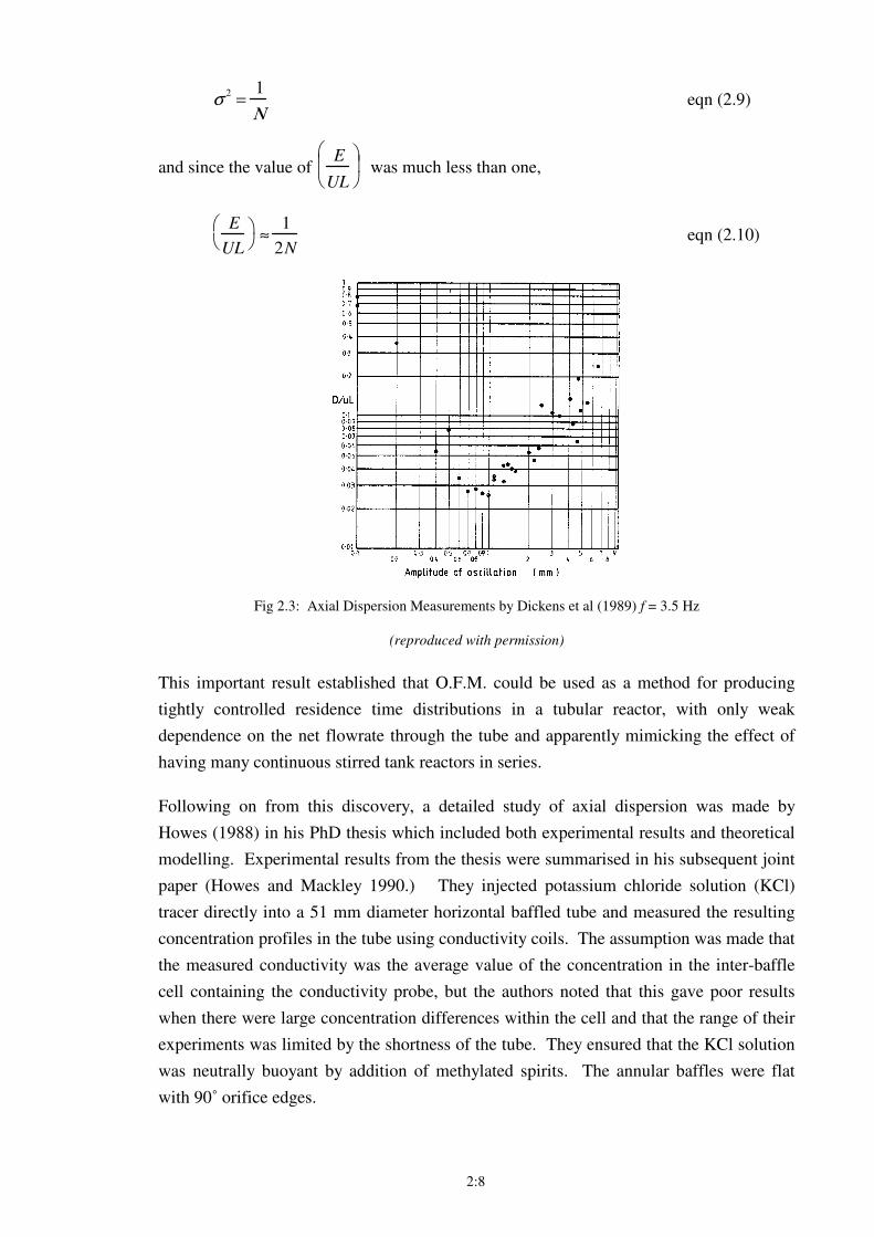
effect of varying amplitude of oscillation on the measured dispersion. They quantified
dispersion using a diffusion model and assumed a perfect pulse of tracer: the variance of
the resulting conductivity trace for each experiment was used to calculate an inverse
Peclet Pe number using the result derived by Levenspiel and Smith (1957):
σ2
= 2E
UL
+ 8
E
UL
2
= 21
Pe
+ 8
1
Pe
2
eqn (2.8)
where σ2
is the calculated variance of the exit concentration profile (see Figure 2.3).
They discovered a minimum value of the inverse Peclet number of about 0.025 which
compared closely with the value that would be obtained using a simple tanks-in-series
model (Levenspiel 1972) where N is the number of perfectly-stirred tanks if it was
assumed that each inter-baffle cavity represented one perfectly-stirred tank:
2:8
σ 2=
1
Ν eqn (2.9)
and since the value of E
UL
was much less than one,
E
UL
≈
1
2N eqn (2.10)
Fig 2.3: Axial Dispersion Measurements by Dickens et al (1989) f = 3.5 Hz
(reproduced with permission)
This important result established that O.F.M. could be used as a method for producing
tightly controlled residence time distributions in a tubular reactor, with only weak
dependence on the net flowrate through the tube and apparently mimicking the effect of
having many continuous stirred tank reactors in series.
Following on from this discovery, a detailed study of axial dispersion was made by
Howes (1988) in his PhD thesis which included both experimental results and theoretical
modelling. Experimental results from the thesis were summarised in his subsequent joint
paper (Howes and Mackley 1990.) They injected potassium chloride solution (KCl)
tracer directly into a 51 mm diameter horizontal baffled tube and measured the resulting
concentration profiles in the tube using conductivity coils. The assumption was made that
the measured conductivity was the average value of the concentration in the inter-baffle
cell containing the conductivity probe, but the authors noted that this gave poor results
when there were large concentration differences within the cell and that the range of their
experiments was limited by the shortness of the tube. They ensured that the KCl solution
was neutrally buoyant by addition of methylated spirits. The annular baffles were flat
with 90˚ orifice edges.
2:9
Howes analysed the concentration data with a tanks-in-series-with-back-mixing model;
the model assumed that each inter-baffle cavity was a perfectly mixed tank with flow to
both the upstream and downstream neighbouring tanks. He presented an algorithm for
calculating a back mixing coefficient and the model could be fitted to give a reasonable
agreement with his experimental dispersion data. Howes performed a series of
experiments in which the tracer was injected either upstream of both probes (an imperfect
pulse technique) or between the probes in order to determine the degree of back-mixing of
the system; he also performed a no-net flow experiment with both probes on one side of
the injection point.
Howes varied Reo , Str and Ren and similarly to Dickens et al (1989) found that imposing
the oscillatory flow upon the steady net flow could substantially reduce the axial
dispersion which could be minimised for a given net flow rate by adjusting the oscillatory
conditions. To explain this phenomenon Howes argued that increasing the oscillatory
flow component would simultaneously increase both the radial and axial mixing in the
tube from which the effect of increasing radial mixing is to reduce axial dispersion while
the effect of increasing axial mixing would serve to increase axial dispersion. Hence
there existed a set of oscillatory conditions for which there would be a balance of radial
and axial mixing to produce a minimum in overall axial dispersion when there was a net
flow present. He also defined a mixing Reynolds number the value of which was
determined from the no-net-flow experiments and which allowed him to predict the value
of oscillation frequency giving minimum dispersion for a given Ren and Str.
Mackley & Ni (1991) injected NaCl solution as a tracer in a 25 mm diameter baffled tube
and measured the changing concentration using point conductivity probes which drew off
a small volume of fluid and which had a reported resolution of about 1mm3. The spatial
resolution of the probes allowed Mackley & Ni to determine differences in the dispersion
as a function of radial position and they concluded that O.F.M. greatly enhanced the radial
distribution of the tracer. The oscillations used by Mackley & Ni (1991) were driven by a
pneumatic cylinder at each end of the closed tube and the authors claimed to have a
square displacement wave form; this unfortunately leaves uncertainty as to the peak
velocity (which in theory must have been infinite!) and creates uncertainty when making a
quantitative comparison with other results.
To quantify the degree of axial dispersion they made use of the diffusion model that is
discussed in detail in §2.2. Their experiments produced similar order-of-magnitude
results to Howes (1990) although using the diffusion model instead of Howes' tanks-in-
series model approach. There was however no satisfactory explanation for the v0ariation
in the measured values of the dispersion coefficient within a particular experiment (three
probes allowed three separate estimates of the axial diffusion coefficient E to be made,
from probes 1→3, 2→3 and 1→2.) Moreover, what should have been a single
parameter diffusion model was effectively made a two-parameter model since both E and
2:10
U were adjusted to fit the model to the data; it is not clear to what extent the values of U
used for calculation in the model differed from reality. In fact, the reason for the
discrepancy between results obtained from the three different sets of probes originated in
incorrect analysis used by the researchers - the correct analysis was identified as part of
this thesis and is dealt with in Chapter 4.
A similar experiment was performed by Mackley & Ni (1993) on a much longer tube of
about 6.3 m with approximately 160 baffles including U-bends. This extra length allowed
measurement of the dispersion in the baffled tube as a function of net flow Reynolds
number without oscillations; a minimum value in the diffusion coefficient was observed
for a net flow Reynolds number of about 400. No evidence was found that the U-bends
affected the axial dispersion. They also reported an experiment using a bundle of five
parallel 25 mm diameter tubes to demonstrate a potential method for scale-up; a reader of
the paper will however observe that there are slight differences in the residence time
distributions for the five tubes which may be indicative of uneven flow distribution to the
five tubes and so probably the method would need some refinement. Ni (1994) presents
similar material.
A rigorous approach to correlating data for axial dispersion in both packed beds and
baffled tubes was presented by Crittenden et al (1995). They proposed equation (2.11) for
curve-fitting:
E
UL= A1 Ren
r+ A2 Reo
mStr
m−q+
A3 Ren2r
A1 Renr + A2 Reo
m Str m− q eqn (2.11)
where A1, A2, A3, m, q and r are constants. They included the results of Dickens et al
(1989) and Howes and Mackley (1990) in their argument to demonstrate the validity of
their equation which was originally developed for packed columns but appeared
potentially valid for O.F.M. as well. The point was not fully proven since the data sets
were incomplete, however their analysis suggested that for a given net flow rate through a
baffled tube the minimum dispersion conditions were achieved when
frequency( )× amplitude( )0.5= constant eqn (2.12)
Using an apparatus similar to that reported in 1991, Ni (1995) made a comparison
between the diffusion model and the tanks-in-series-with-backmixing model for the data
analysis. For each model, he calculated a value for the Peclet number and found
discrepancies in the value depending upon which model was used. This was most likely
the result of using an inappropriate solution to the diffusion equation for the particular
boundary conditions, as has previously been noted.
Stonestreet (1997) also investigated residence time distributions in a 24 mm diameter
baffled tube with oscillations, and concluded that as a rule-of-thumb the axial dispersion
2:11
could be minimised for a given net flow if the oscillatory Reynolds number was in the
range between two to five times greater in magnitude than the net flow Reynolds number.
This applied to net flows in the range 50 ≤ Ren ≤ 300.
2.1.5 Numerical Simulation Studies of O.F.M.
The majority of the numerical simulation work performed on O.F.M. has taken place
under the supervision of M.R. Mackley at the Department of Chemical Engineering,
Cambridge University, and was initiated by T. Howes during his doctoral research in the
form of a finite difference model run on Fortran code. Subsequent researchers at the
Department (Roberts and Neves Saraiva) have developed these algorithms further and
have generously made them available to other researchers, including the author of this
thesis in which the code has been used to simulate streaklines, velocity maps and
dispersion.
Two-dimensional axisymmetric numerical flow simulations for steady and oscillatory
flow patterns in a baffled tube were made by Howes (1988) who compared the results to
experimentally obtained flow visualisation photographs. These flow visualisations were
obtained via the method adopted by Brunold et al (1989) using timed-exposure
photographs of the flow containing neutrally-buoyant 100 micron polyethylene particles
with slit-illumination to produce streaklines through a cross-section of the flow. Howes
developed a finite-difference model based on Fortran code to simulate the dispersion of
fluid marker particles within the simulation, the results of which he could then compare
with experimental data. The flow was experimentally found to be axisymmetric for
Reo less than about 300 in the geometry studied and simulations matched experimental
observations well for Reo ≤ 200.
The nature of the flow at low Reo is that vortices are formed behind the baffles, grow, and
then are ejected towards the centre of the tube when the flow direction reverses,
eventually dissipating. At higher Reo (above 300) the vortices interact, breaking the
axisymmetry and forming chaotic flow patterns. Howes' calculated flow patterns were
unable to predict such complex flow and were therefore limited to flows with Reo ≤ 200.
Numerically generated two-dimensional flow visualisations of flow without oscillations
in a two-dimensional baffled channel using a particle mapping technique were reported by
Howes, Mackley & Roberts (1991) which predicted a critical Ren between 100 and 200 at
which the flow becomes unsteady and the symmetry of the flow pattern is broken. A
similar critical value for Reo was also discovered and the model was thought valid up to
Reo = 700 . They noted that so long as Ren ≤ Reo then the oscillations would have a
useful effect in increasing chaotic mixing.
2:12
Wang et al (1994) examined numerical simulations for either wall or central baffles and
they observed that the vortex strength was stronger for wall baffles; there was a
maximum of vortex strength at a Strouhal number (inversely proportional to oscillatory
amplitude) of approximately unity.
Kinematic mixing rates in a baffled tube were calculated by Mackley & Roberts (1995)
who observed that for oscillatory flow the mixing rate was well distributed over the flow
field for Reo ≥ 80 . They used both a particle separation approach and a stretch rate
approach to describe the mixing. Under oscillatory conditions Str = 1 and Reo = 60 or 80
they predicted optimum stretch rates at baffle spacings of 0.6 and 0.9 channel diameters
respectively. It seems therefore that for optimum mixing conditions, the baffle geometry
should ideally be tailored to the particular oscillatory conditions.
The work of Howes, Roberts and Mackley was further developed by Saraiva (1997) who
in his PhD thesis presents mainly theoretical results related to mixing in O.F.M. at low
Reynolds numbers for axisymmetric flows, both for mixing in the region between baffles
(intra-cell mixing rates) and for the mixing between regions separated by baffles (inter-
cell mixing rates.) He examined two different methods for quantifying the intra-cell
mixing rate (firstly a fluid element deformation method and secondly a concentration-time
evolution tracer injection method) and concluded that there was a direct correlation
between the two methods. He studied the effect of baffle spacing on mixing performance
and concluded that for the conditions Ren = 0, Reo = 100 and Str = 1 the mixing rate was
only a weak function of baffle spacing: there was a weak maximum at a baffle spacing of
around 2 tube diameters but remained substantially unchanged between 1.25 and 2.75
diameters spacing. In collaboration with the work carried out in this thesis, he also
carried out modelling on manifolds in O.F.M. and used experimental results from this
thesis to substantiate his values for axial dispersion obtained by fluid-mechanical
modelling. Saraiva also showed that molecular diffusion (of a salt tracer in water) only
made a significant contribution to the overall measured axial dispersion for oscillatory
Reynolds numbers of less than approximately 100.
2:13
2.2 Measurement and Modelling of Axial Dispersion
Axial dispersion is a measure of the rate at which an inert tracer spreads axially along a
tube such as is found in O.F.M.. It can be a measure of macro-mixing (e.g. mechanical
mixing of the bulk fluid) or of micro-mixing (e.g. molecular diffusion) or most
commonly a combination of both types of mixing. Quantification of axial dispersion is of
particular interest for tubular-style reactors since the results can then be used to predict
residence time distributions for either larger or smaller reactors.
Several different models for axial dispersion are presented in the literature; in this thesis
the "diffusion equation" is the primary model chosen for the quantification of axial
dispersion from experimental data.
This section is divided into three parts. The first (§2.2.1) discusses the various models
available to quantify axial dispersion and their suitability to the problem of O.F.M.. In
§2.2.2 the solutions to the diffusion equation presented in the literature are treated in more
detail, and conflicting results are highlighted. Finally, §2.2.3 deals with methods used by
researchers to estimate axial dispersion using fluid mechanical simulations, particularly in
flow regimes where regular experimental techniques have proved inadequate.
2.2.1 Models Available for Quantification of Axial Dispersion
The two principal models adopted in the literature to describe dispersion in O.F.M. are
i) The diffusion model, and
ii) The tanks-in-series model, with or without backmixing.
The diffusion model uses the analogy of molecular diffusion to describe macro-mixing
and was first used as a model for axial dispersion in O.F.M. by Mackley & Ni (1991). So
as (hopefully) to avoid confusion this thesis will use the symbol E for axial diffusion and
the symbol D for molecular diffusion. The mathematics of the diffusion model are dealt
with in detail in §2.2.2.
The diffusion model is inherently appropriate for describing a physical situation where
homogenous mixing exists (Levenspiel 1972). It may therefore be supposed that it is a
good model for O.F.M. when substantial mixing occurs (i.e. under chaotic mixing
conditions) but that it may fail if there are large segregated volumes of fluid in the flow
(for example at low Reynolds number flows). The model has the advantages that it is in
common usage (and therefore familiar to most chemical engineers) and has been well-
studied for a variety of boundary conditions. A potential disadvantage of the diffusion
2:14
model with respect to O.F.M. is that it takes no account of the geometry of O.F.M. (i.e.
the presence of periodically-spaced baffles which compartmentalise the flow.)
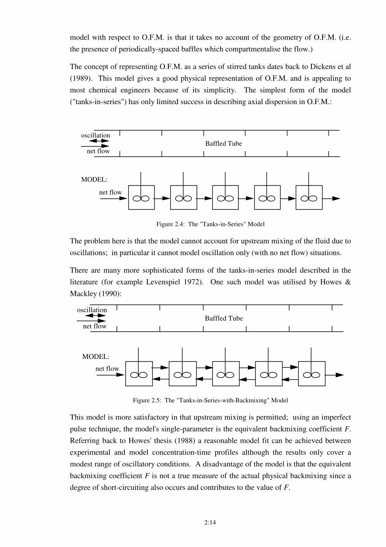
The concept of representing O.F.M. as a series of stirred tanks dates back to Dickens et al
(1989). This model gives a good physical representation of O.F.M. and is appealing to
most chemical engineers because of its simplicity. The simplest form of the model
("tanks-in-series") has only limited success in describing axial dispersion in O.F.M.:
oscillation
net flow
net flow
Baffled Tube
MODEL:
Figure 2.4: The "Tanks-in-Series" Model
The problem here is that the model cannot account for upstream mixing of the fluid due to
oscillations; in particular it cannot model oscillation only (with no net flow) situations.
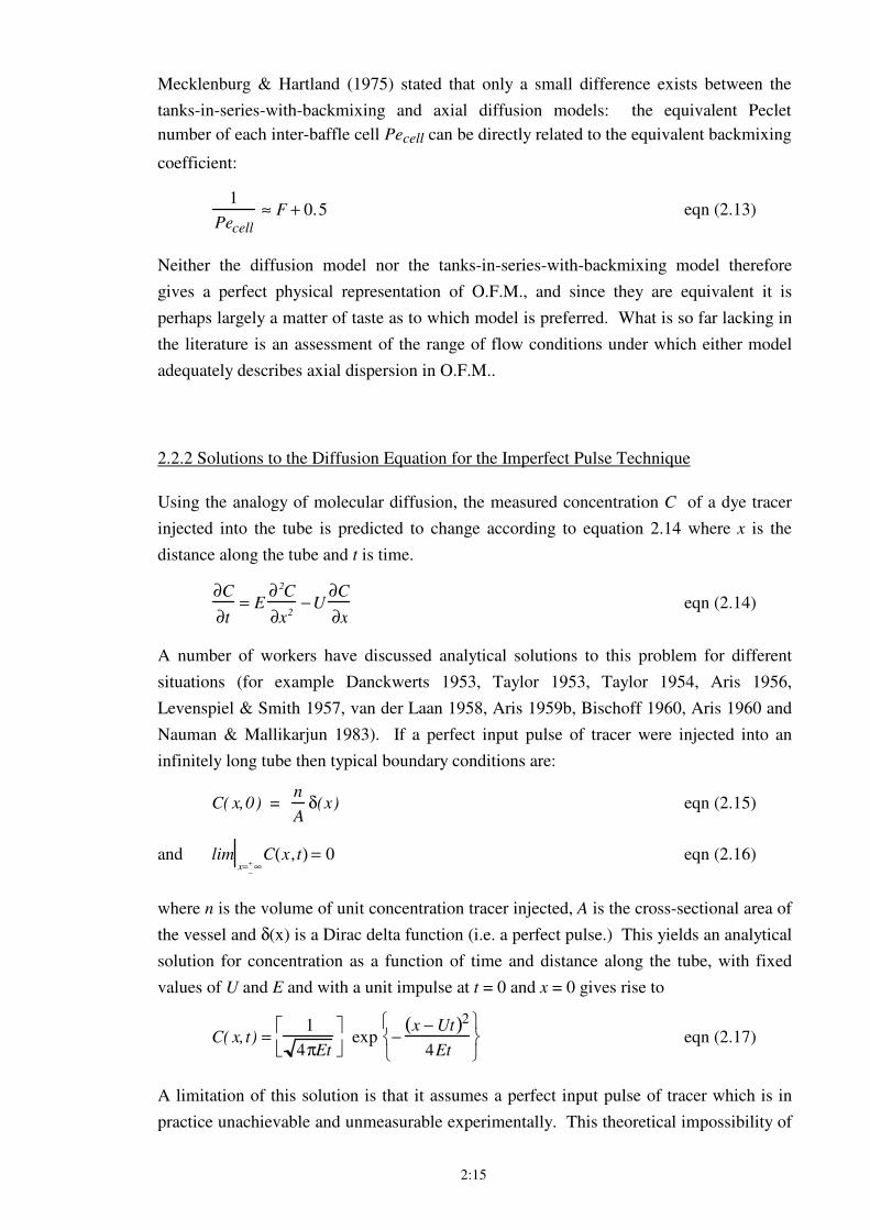
There are many more sophisticated forms of the tanks-in-series model described in the
literature (for example Levenspiel 1972). One such model was utilised by Howes &
Mackley (1990):
oscillation
net flow
net flow
Baffled Tube
MODEL:
Figure 2.5: The "Tanks-in-Series-with-Backmixing" Model
This model is more satisfactory in that upstream mixing is permitted; using an imperfect
pulse technique, the model's single-parameter is the equivalent backmixing coefficient F.
Referring back to Howes' thesis (1988) a reasonable model fit can be achieved between
experimental and model concentration-time profiles although the results only cover a
modest range of oscillatory conditions. A disadvantage of the model is that the equivalent
backmixing coefficient F is not a true measure of the actual physical backmixing since a
degree of short-circuiting also occurs and contributes to the value of F.
2:15
Mecklenburg & Hartland (1975) stated that only a small difference exists between the
tanks-in-series-with-backmixing and axial diffusion models: the equivalent Peclet
number of each inter-baffle cell Pecell can be directly related to the equivalent backmixing
coefficient:
1
Pecell
≈ F + 0.5 eqn (2.13)
Neither the diffusion model nor the tanks-in-series-with-backmixing model therefore
gives a perfect physical representation of O.F.M., and since they are equivalent it is
perhaps largely a matter of taste as to which model is preferred. What is so far lacking in
the literature is an assessment of the range of flow conditions under which either model
adequately describes axial dispersion in O.F.M..
2.2.2 Solutions to the Diffusion Equation for the Imperfect Pulse Technique
Using the analogy of molecular diffusion, the measured concentration C of a dye tracer
injected into the tube is predicted to change according to equation 2.14 where x is the
distance along the tube and t is time.
∂C
∂t= E
∂ 2C
∂x2−U
∂C
∂x eqn (2.14)
A number of workers have discussed analytical solutions to this problem for different
situations (for example Danckwerts 1953, Taylor 1953, Taylor 1954, Aris 1956,
Levenspiel & Smith 1957, van der Laan 1958, Aris 1959b, Bischoff 1960, Aris 1960 and
Nauman & Mallikarjun 1983). If a perfect input pulse of tracer were injected into an
infinitely long tube then typical boundary conditions are:
C( x,0) = n
Aδ(x) eqn (2.15)
and limx=
−
+ ∞C(x, t) = 0 eqn (2.16)
where n is the volume of unit concentration tracer injected, A is the cross-sectional area of
the vessel and δ(x) is a Dirac delta function (i.e. a perfect pulse.) This yields an analytical
solution for concentration as a function of time and distance along the tube, with fixed
values of U and E and with a unit impulse at t = 0 and x = 0 gives rise to
C( x,t) =1
4πEt
exp −
x − Ut( )2
4Et
eqn (2.17)
A limitation of this solution is that it assumes a perfect input pulse of tracer which is in
practice unachievable and unmeasurable experimentally. This theoretical impossibility of
2:16
achieving perfect pulse injection can be avoided by the use of the imperfect pulse method
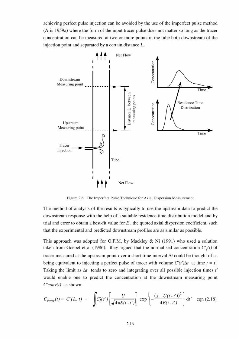
(Aris 1959a) where the form of the input tracer pulse does not matter so long as the tracer
concentration can be measured at two or more points in the tube both downstream of the
injection point and separated by a certain distance L.
Tracer
Injection
Net Flow
Dis
tan
ce L
bet
wee
n
mea
suri
ng
po
ints
Downstream
Measuring point
Net Flow
Co
nce
ntr
atio
n
Time
Co
nce
ntr
atio
n
Time
Residence Time
Distribution
Upstream
Measuring point
Tube
Figure 2.6: The Imperfect Pulse Technique for Axial Dispersion Measurement
The method of analysis of the results is typically to use the upstream data to predict the
downstream response with the help of a suitable residence time distribution model and by
trial and error to obtain a best-fit value for E , the quoted axial dispersion coefficient, such
that the experimental and predicted downstream profiles are as similar as possible.
This approach was adopted for O.F.M. by Mackley & Ni (1991) who used a solution
taken from Goebel et al (1986): they argued that the normalised concentration C'1(t) of
tracer measured at the upstream point over a short time interval ∆t could be thought of as
being equivalent to injecting a perfect pulse of tracer with volume C'(t')∆t at time t = t'.
Taking the limit as ∆t tends to zero and integrating over all possible injection times t'
would enable one to predict the concentration at the downstream measuring point
C'conv(t) as shown:
′ C conv(t) = ′ C (L, t) = ′ C 1(t' )
0
t
∫ U
4πE(t - t' )
exp −
x −U(t - t' )( )2
4E(t - t' )
dt' eqn (2.18)
2:17
which is a convolution integral and must be integrated numerically. The value of the
diffusion coefficient E was adjusted iteratively to give the best fit between C'conv and the
measured concentration C'2 using either a least squares algorithm or by visual inspection.
[The latter method is anyway a wise precaution since it can quickly be seen if there is a
large discrepancy between the shape of the profiles].
From equation 2.18 can be extracted the transfer function between measuring points one
and two (effectively the residence time distribution between the two measuring points
with open-open boundaries):
TransferFunction(t) = U
4πEt
exp −
x − Ut( )2
4Et
eqn (2.19)
This is however in disagreement with the transfer function proposed by Scott (1997):
TransferFunction(t) = 1
4πEt3
x2
exp −x − Ut( )2
4Et
eqn (2.20)
which is equivalent to the solution given for the same boundary conditions by Westerterp
et al (1984) who gave the same transfer function in terms of dimensionless time θ and the
Peclet number:
TransferFunction(θ) = Pe
4πθ 3 exp −Pe 1 −θ( )2
4θ
eqn (2.21)
where θ =tU
L eqn (2.22)
Equations 2.19 (after Goebel et al 1986) and 2.20 (after Westerterp et al 1984) both
purport to describe the same situation and are of similar mathematical form, but there is a
subtle difference in the pre-exponential term which renders them different. This apparent
conflict is examined in Chapter 4.
2.2.3 Estimates of Axial Dispersion from Fluid Mechanical Simulations
A large body of literature exists for the experimental quantification of axial dispersion as
has been demonstrated in the preceding sections of this chapter. It was found during the
course of this thesis that because of the nature of the flow observed in O.F.M. at very low
Reynolds numbers (especially channelling of the flow), the axial diffusion model was
inadequate under some circumstances. Nevertheless a method was still sought to quantify
axial dispersion under these conditions.
2:18
In recent years advances in computing power have made it possible to perform numerical
fluid mechanical simulations of entire flow fields. Sobey (1985) used a fluid mechanical
simulation to estimate axial dispersion in wavy-walled channels. In conjunction with his
fluid mechanical simulation he advected a large number of fluid marker particles within
one cell and monitored the variance of the particles' axial position from which the
dispersion coefficient could be directly calculated.
Sobey’s method was adopted by Howes (1988) who advected fluid marker particles
within his fluid mechanical simulation to determine axial dispersion in O.F.M.. Howes’s
simulation was based upon a fluid mechanical simulation of the velocity field in O.F.M.
together with the superposition at the end of each oscillatory cycle of a random-walk
concept to model molecular diffusion (without which the marker particles would be
trapped in certain domains). The model gave satisfactory results for axial dispersion
using the method of moments (Aris 1956). The method relies however on the assumption
that the rate of increase of variance of the particle cloud is constant. At very low values
of Ren with some net component to the flow, he found that it took many oscillatory cycles
before the rate of increase of variance was constant. In order to speed up the calculations
he therefore used a transfer function method (based upon a method for determining
dispersion in tidal estuaries) which only required knowledge of the position of the
particles at a single point in time for an oscillatory cycle. The transfer function was
therefore used to compute the change in position over one oscillatory cycle of any particle
in a single inter-baffle cell.
Howes’s fluid mechanical simulation was further developed by Saraiva (1997) who
utilised the advection of inert fluid marker particles to measure both axial dispersion and
mixing in O.F.M.. He quantified axial dispersion using equation 2.23 for the case of
oscillatory flow only, for which the rate of change of variance was constant soon after the
simulated injection of the particles.
E =t→ ∞lim
1
2
d < (x(t)− < x(t) >) 2 >
dt eqn (2.23)
where x(t) is the axial position of each marker particle as a function of time (averaged
over one oscillatory cycle) and the angular brackets represent an average over all the
marker particles. In dimensionless form the relationship between axial dispersion and
particle variance becomes:
1
Sc=
ρE
µ=
t →∞lim
ReoStr
4
d < (x(t)− < x(t) >)2 >
dt eqn (2.24)
This method is not applicable to practical experiments since knowledge of the complete
tracer distribution at an instant in time is required. A variant of the method can be used
2:19
for experimental purposes (see for example Dickens et al 1989) but is prone to large
errors resulting from small inaccuracies in the measurement of tracer concentration.
In conjunction with the work in this thesis Saraiva also adapted the simulation to be
capable of mapping inert tracer particles so as to mimic the effect of inert dye injection in
a practical experiment. Moreover, the mean cross-sectional concentration of these marker
particles could be determined in a manner analogous to the optical concentration sensors
used in this thesis (Hwu et al 1996). This allowed direct substitution of simulated
residence time distributions into the analysis programme developed for the interpretation
of experimental residence time distribution measurements as part of this thesis (Chapter
4).
2.3 Studies Of Systems Analogous To O.F.M.
This section is not intended as a comprehensive review of pulsed packed beds and
reciprocating plate columns, but aims to high-light similarities with O.F.M. in respect of
axial dispersion measurements, modelling and scale-up. It is divided into two sections,
dealing respectively with the relevant literature on pulsed packed beds (§2.3.1) and
reciprocating plate columns (§2.3.2).
2.3.1 Pulsed Packed Beds
Pulsed packed beds typically consist of a tube filled with small to medium sized particles
or beads, through which a continuous flow of liquid is pumped with superimposed
oscillations. There are a number of similarities between the behaviour of pulsed packed
beds and O.F.M. and some of the observations from pulsed packed beds can probably be
applied to the latter. The diffusion model is particularly relevant since the packed bed can
be thought of as homogeneous rather than having discrete regions.
In 1958 Carberry & Bretton reported experiments on axial dispersion in steady flow
through packed beds in a 38 mm diameter column using a range of packings and a dye-
tracer technique. They discovered that axial dispersion increased linearly with Reynolds
number (based upon the diameter of the packing and the fluid properties) up to a
Reynolds number of about 100, i.e. E ∝ Ren . At higher net flows, the dependence reduced
until E ∝ Ren
0 .25 at a critical Reynolds number of around 400. This makes an interesting
comparison with the findings of Mackley & Ni (1993) for oscillatory flow where they
observed a minimum in axial dispersion for steady net flows of Reynolds number
approximately 400. Carberry & Bretton also reported larger axial dispersion than
2:20
predicted by diffusion theory and concluded that this was due to bed-capacitance. Their
experiments also showed higher dispersion in shorter beds.
Axial dispersion in a 50 mm diameter by 4 m long pulsed packed column was measured
by Goebel et al (1986) using potassium chloride salt solution tracer and an imperfect
pulse technique. They plotted their data as a graph of E
u'd p
against 4πωx0
u'where u' is
the mean interstitial velocity and dp is the packing diameter. The first group is therefore
similar to an inverse Peclet number and the latter group is a ratio of the oscillatory and net
flow velocities. The data showed a characteristic minimum value for E
u'd p
as a function
of 4πωx0
u'. This concept of relative importance of oscillatory and net flows may be a
useful method for describing flows in O.F.M., although very low net flows are of primary
interest for the design of long residence time reactors.
Pulsed packed columns ranging from 50 mm to 2400 mm diameter were examined by
Simons et al (1986). They used both KCl solution and a radioactive indium tracer to
measure axial dispersion. Importantly, they determined that axial dispersion E was a
function of ωx0 and geometry only, and not a function of column diameter as had been
suggested by previous workers.
Axial dispersion data from a 50 mm packed column was correlated by Mak et al (1991)
who found that for 0 < Ren < 180 and 0 < Reo < 600 the dependence of E was given by:
Eρ
µ= A1Ren
n+ A2Reo +
A3Ren
2n
A1 Ren
n+ A2 Reo
eqn (2.25)
which is very similar in form to eqn (2:11) from Crittenden et al (1995) although the latter
is slightly more refined in its approach in that it separates the dependence of E with
respect to amplitude and frequency of oscillation.
2.3.2 Reciprocating Plate Columns
Reciprocating plate columns are most often used for contacting immiscible liquids for
separation processes and as such are well described by Long (1967). Some axial
dispersion work has nevertheless been carried out in a liquid single phase system and this
is of interest because of the stage-wise partitioning of the column which is comparable to
the geometry of O.F.M.. Reciprocating plate columns contain stacks of multi-orifice
plates that are oscillated at around 1Hz and with an amplitude of a few mm. The orifices
are of the order of 12 mm diameter and the total area constriction of the plate is typically
50%. [Note that pulsed plate columns are generally considered to have smaller orifices of
2:21
around 2 mm diameter and operate on a mixer-settler principle for immiscible liquid
contacting; these are not discussed.]
A reciprocating plate column of 150 mm diameter was examined by Baird (1974) who
used the colour change acid-base reaction to indicate axial dispersion. Interestingly, for
coarsely perforated plates the dispersion was proportional to amplitude2
× frequency but
semicircular unperforated plates showed a dependence on amplitude × frequency and the
author comments upon the excellent radial mixing with this kind of baffle. The latter
could be considered to be closest in nature to single orifice baffles in O.F.M..
A 50 mm diameter reciprocating plate column was studied by Kim & Baird (1976a).
They surprisingly discovered that the Teflon baffles (3.4 mm thick) produced significantly
lower axial dispersion than with stainless steel baffles (1.5 mm thick) for which E was
more than 30% larger; they repeated the experiments with double-thickness steel baffles
(to give approximately the same total baffle thickness as for the Teflon) for which the
axial dispersion was then the same as for Teflon, from which they reasonably concluded
that the baffle thickness was a parameter affecting axial dispersion.
They also observed that increasing the viscosity of the fluid (by a factor of 4 using glucose
syrup in water) had negligible effect upon the value of the dispersion coefficient from
which they concluded that viscous effects were unimportant in the essentially turbulent
nature of the flow. Orifice diameter was 14 mm and the oscillatory conditions were 0.5 to
6 Hz and 6 to 22 mm centre-to-peak amplitude. Column diameter also had little effect on
axial dispersion. These results may not hold as well for O.F.M. operating at low
Reynolds flow in which case viscous effects may become important. Kim & Baird also
varied plate spacing H as a parameter and correlated their results for a wide range of
oscillatory conditions. They plotted the data on a single graph with the correlation
E ∝xo
1.74ω0.96
H0.69 . The notation has been adjusted to be consistent with this dissertation; the
dependence of E almost proportional to frequency but with a power-relationship to
amplitude is interesting.
In a subsequent paper (Kim & Baird 1976b) they examined further the effect of orifice
diameter c, plate thickness T and separation H and concluded that E ∝xo
1.8ω1.0c1.8
H1.3
T0.3 . They
found that halving c with plate free area kept constant reduced the amount of axial
dispersion by about 75%. The dependance upon H appeared to be strongly related to the
precise baffle geometry.
A model for axial dispersion suggested by Stevens & Baird (1990) considered that the
region swept out by the plates was very well mixed but with relatively poor mixing
between the plates; the model could in principle be applied to O.F.M..
2:22
A review paper (Lo et al 1992) noted from the literature a power-law dependence of the
form E ∝ dn where d is the column diameter and n is between 0.3 and 0.67 depending
upon plate geometry.
Baird (1996) reported axial dispersion measurements in a 150 mm diameter reciprocating
plate column employing single orifice baffles with a constriction of approximately 75%
for which E was found to be proportional to Reo. Although measurements were only
made at high Reynolds numbers (8000 and above), the results can be directly compared
with experiments carried out as part of this thesis (but with oscillating fluid rather than
oscillating baffles as the only substantial difference.)
Lounes & Thibault (1996) investigated axial dispersion using KCl tracer in a 0.1 m
diameter batch reciprocating plate column with multi-orifice baffles with orifice diameter
6.25 mm and a total baffle constriction of 72%. From their experiments they concluded
that axial dispersion E ∝ xo0.756ω 1.066
.
It is concluded that nearly all the correlations for reciprocating plate columns available in
the literature predict axial dispersion to be approximately proportional to frequency but
for amplitude of oscillation the correlations vary from E ∝ xo0.756
to E ∝ xo2
.
3:1
3. Apparatus and Experimental Method
In order to study the effect of scale-up on Oscillatory Flow, three sets of geometrically
similar apparatus were designed and constructed. The smallest apparatus was a 1 m tall
tube of 24 mm internal diameter and the largest was a 4.5 m tall tube of 150 mm internal
diameter. In conjunction with the design and construction of the apparatus, experimental
methods were developed for flow visualisation (using fluorescent dye streaklines) and
measurement of residence time distributions (using dye tracer and optical sensors) which
could be applied to all three sets of apparatus in order to give directly comparable results
between different scales.
The design and construction of the sets of apparatus as well as the selection and
development of experimental techniques formed a significant part of the work presented
in this thesis and are therefore described in detail: §3.1 discusses the design criteria and
construction of the experimental apparatus; §3.2 describes the selection and
implementation of the experimental methods used.
3.1 Design Criteria and Construction of Apparatus
In setting out to design apparatus to test scaling laws for a particular reactor geometry,
consideration was given to the likely requirements of oscillation and physical size as one
moves to a larger or smaller scale; these requirements placed potential restrictions upon
the maximum scale of apparatus that could reasonably be constructed. This discussion is
set out in §3.1.1, followed by a description of the actual construction of the apparatus in
§3.1.2. For clarity, some of the construction detail is presented more fully in the
Appendices.
3.1.1 The Required Range of Operating Conditions for the Apparatus
Most experimental investigations of O.F.M. to date have concentrated upon tubes of
approximately 24 mm or 51 mm internal diameter (see Table 2.1). In order that
comparisons could be made with other studies of O.F.M. (for example investigations into
axial dispersion or suspension of particles) it was decided to construct geometrically
similar sets of apparatus of 24 mm and 54 mm internal diameter (using standard clear
acrylic tubing). For industrial applications it is likely that larger tube diameters would
have to be considered in order to accommodate large throughputs and it was therefore
decided to construct a third larger apparatus which would be comparable in size to
industrial or pilot-scale apparatus.
3:2
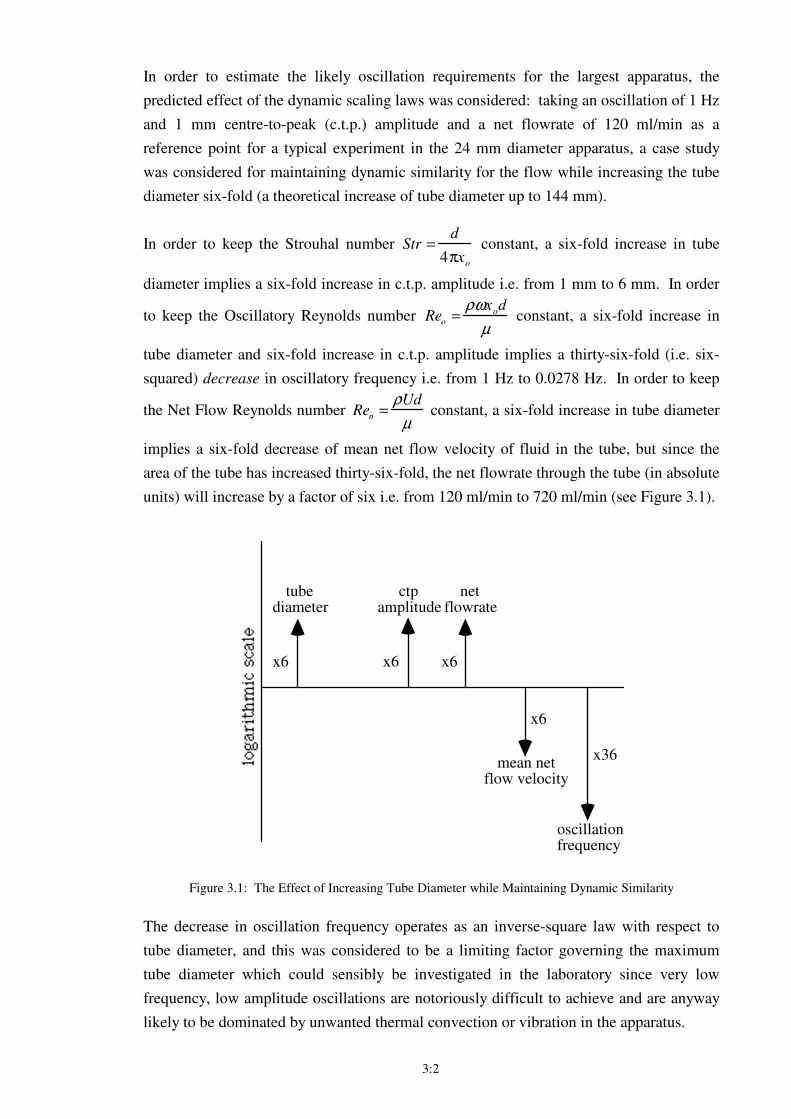
In order to estimate the likely oscillation requirements for the largest apparatus, the
predicted effect of the dynamic scaling laws was considered: taking an oscillation of 1 Hz
and 1 mm centre-to-peak (c.t.p.) amplitude and a net flowrate of 120 ml/min as a
reference point for a typical experiment in the 24 mm diameter apparatus, a case study
was considered for maintaining dynamic similarity for the flow while increasing the tube
diameter six-fold (a theoretical increase of tube diameter up to 144 mm).
In order to keep the Strouhal number Str =d
4πxo
constant, a six-fold increase in tube
diameter implies a six-fold increase in c.t.p. amplitude i.e. from 1 mm to 6 mm. In order
to keep the Oscillatory Reynolds number Reo
=ρωx
od
µ constant, a six-fold increase in
tube diameter and six-fold increase in c.t.p. amplitude implies a thirty-six-fold (i.e. six-
squared) decrease in oscillatory frequency i.e. from 1 Hz to 0.0278 Hz. In order to keep
the Net Flow Reynolds number Ren
=ρUd
µ constant, a six-fold increase in tube diameter
implies a six-fold decrease of mean net flow velocity of fluid in the tube, but since the
area of the tube has increased thirty-six-fold, the net flowrate through the tube (in absolute
units) will increase by a factor of six i.e. from 120 ml/min to 720 ml/min (see Figure 3.1).
x6 x6 x6
x6
x36
tube diameter
ctp amplitude
net flowrate
mean net flow velocity
oscillation frequency
Figure 3.1: The Effect of Increasing Tube Diameter while Maintaining Dynamic Similarity
The decrease in oscillation frequency operates as an inverse-square law with respect to
tube diameter, and this was considered to be a limiting factor governing the maximum
tube diameter which could sensibly be investigated in the laboratory since very low
frequency, low amplitude oscillations are notoriously difficult to achieve and are anyway
likely to be dominated by unwanted thermal convection or vibration in the apparatus.
3:3
In contrast to net flow, amplitude and frequency, it was predicted from the Schmidt
number Sc =µ
ρE that the absolute value of the axial dispersion coefficient E would be
independent of scale since µ and ρ are properties of the fluid only. This was also
consistent with the Peclet number Pe =UL
E where the relative changes in U and L (with
respect to tube diameter) are inversely proportional to one another and therefore the value
of E should be independent of scale assuming that the dynamic flow conditions were
similar. This was a surprising prediction, since it might otherwise have been assumed
intuitively that the axial dispersion would be greater in magnitude for larger diameter
tubes.
In order that the sets of apparatus should be geometrically similar to one another, the
aspect ratio of the tube (height to diameter) was designed to be approximately constant.
In addition, in order to avoid the possibility of end-effects substantially altering the results
(since the analysis to be used would assume an infinitely long tube, see §3.2) a minimum
number of baffles were required in the tube. In practice, the tallest lab-space available
was 5 m, which allowed for 18 baffles spaced at 1.5 times the tube diameter for a vertical
150 mm internal diameter tube (making allowance for the oscillator at the base of the
tube.) Horizontal tubes or tubes with multiple bends were also considered in order to
achieve a greater tube length, but it was determined from small-scale trials that these
would not only lead to significant problems of degassing of trapped air but also, as
discussed in §3.2, offered negligible benefit to the accuracy of residence time distribution
experiments when using an imperfect pulse technique.
Practical height considerations therefore limited the largest tube diameter which could be
investigated to 150 mm, and as already discussed the necessarily low oscillation
frequencies (down to less than one cycle per minute for 150 mm tubes) in order to achieve
dynamic similarity for the same fluid as in a 24 mm tube, also prohibited the investigation
of any larger diameter tubes. The use of a more viscous fluid (such as sugar solution,
Saraiva 1997) to avoid these low frequency oscillations was considered but rejected
because of the very large amounts of fluid involved: requiring up to approximately 300
litres of fluid per experiment, the only practical fluid for the 150 mm diameter apparatus
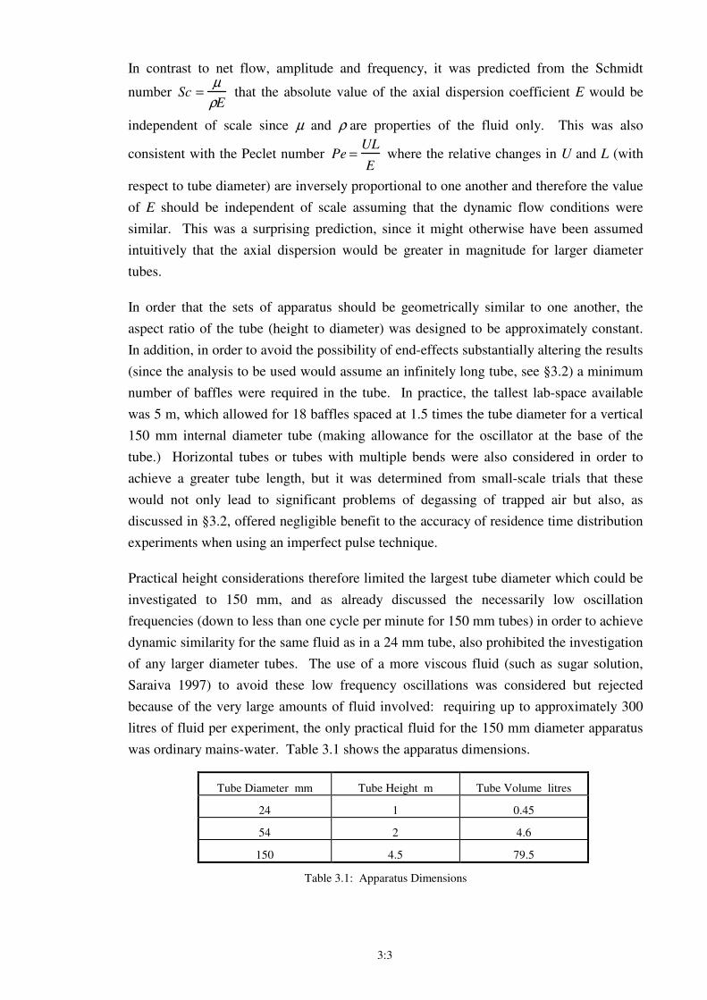
was ordinary mains-water. Table 3.1 shows the apparatus dimensions.
Tube Diameter mm Tube Height m Tube Volume litres
24 1 0.45
54 2 4.6
150 4.5 79.5
Table 3.1: Apparatus Dimensions
3:4
3.1.2 Construction of the Apparatus
All of the apparatus was self-designed and constructed in-house from a combination of
off-the-shelf and self-engineered components (with the exception of the perspex viewing-
boxes which were manufactured by the Department of Chemical Engineering Workshop.)
As has been discussed in §3.1.1, one of the major potential difficulties of performing
dynamically similar experiments at different scales was the very low oscillation
frequencies (of the order 0.01 Hz) required for the larger diameter apparatus. At the same
time, the apparatus needed also to be capable of higher frequency oscillations (of the order
10 Hz) in order to explore the full effect of different conditions. With such a wide range
of frequencies required, any motor-driven system would have required very substantial
changeable gearing to be able to drive a smooth sinusoidal oscillation. (The mass of fluid
to be oscillated in the 150 mm apparatus was approximately 80 kg, so inertial effects were
important as well as any pressure drop across the baffles.) Motor or stepper-motor with
cam-follower oscillators were therefore discounted because of the likely gearing and
vibration problems and consequent expense.
Electromagnetic moving-coil oscillations were also considered for the 150 mm apparatus
but rejected because of their limited power (and considerable expense) and because of
their very limited stroke-length. For smaller apparatus however they are an ideal
oscillator and a moving-coil oscillator was used to drive oscillations in the smallest (24
mm diameter) apparatus, having sufficient power and stroke-length to drive a wide range
of oscillation frequencies.
Pneumatic pistons were considered for the larger rigs but were rejected because of the
severe control problems inherent with oscillating large masses by means of a
compressible gas. Another possibility for an industrial system would be direct pressurised
air pulsing in a manometer-style tube as described by Baird (1966); such a system would
be cheap to install but is limited in performance unless operating close to the resonant
frequency of the system, as well as having safety concerns in the laboratory due to being
effectively a large volume pressure vessel.
Finally, servo-hydraulics were selected as the most appropriate and cost-effective method
of providing oscillations for the 54 mm and 150 mm diameter experimental apparatus;
this was the first time that servo-hydraulics had been employed in O.F.M. but were
nevertheless successfully implemented and proved to be highly reliable. The hydraulics
were constructed from off-the-shelf components which could easily be interchanged or
replaced and moreover the hydraulic power unit (supplying high pressure hydraulic oil to
a piston) and control electronics could be shared between the 54 mm and 150 mm
apparatus since only one or other apparatus was operated at any one time. The only
duplication of equipment was therefore the individual hydraulic cylinders and
displacement transducers assigned to each apparatus, tailored to the individual
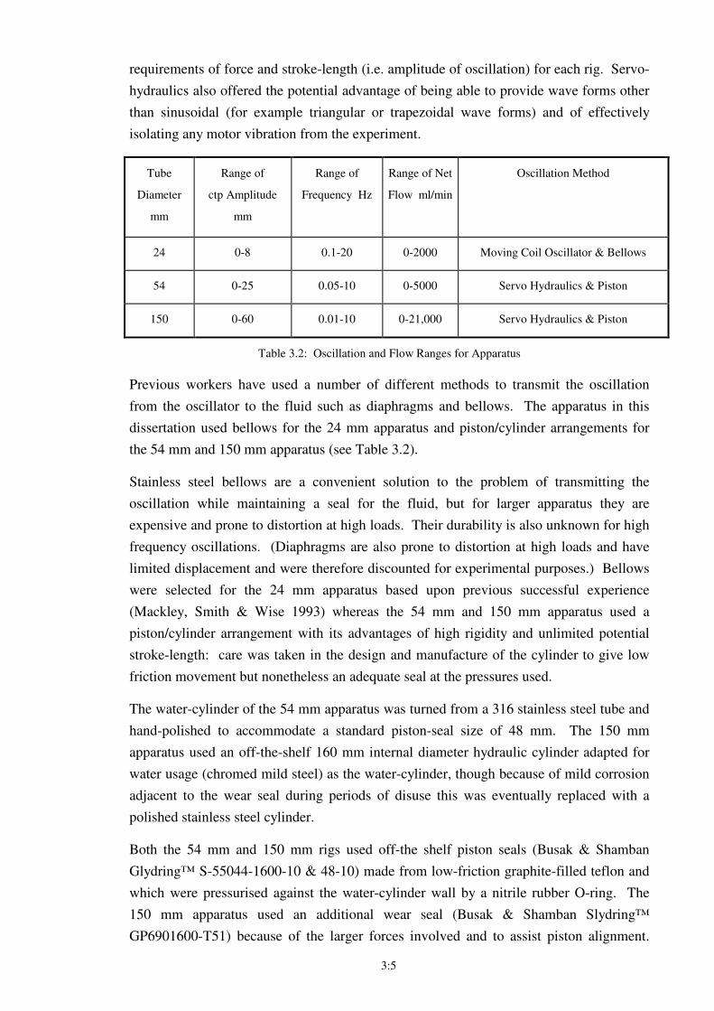
3:5
requirements of force and stroke-length (i.e. amplitude of oscillation) for each rig. Servo-
hydraulics also offered the potential advantage of being able to provide wave forms other
than sinusoidal (for example triangular or trapezoidal wave forms) and of effectively
isolating any motor vibration from the experiment.
Tube
Diameter
mm
Range of
ctp Amplitude
mm
Range of
Frequency Hz
Range of Net
Flow ml/min
Oscillation Method
24 0-8 0.1-20 0-2000 Moving Coil Oscillator & Bellows
54 0-25 0.05-10 0-5000 Servo Hydraulics & Piston
150 0-60 0.01-10 0-21,000 Servo Hydraulics & Piston
Table 3.2: Oscillation and Flow Ranges for Apparatus
Previous workers have used a number of different methods to transmit the oscillation
from the oscillator to the fluid such as diaphragms and bellows. The apparatus in this
dissertation used bellows for the 24 mm apparatus and piston/cylinder arrangements for
the 54 mm and 150 mm apparatus (see Table 3.2).
Stainless steel bellows are a convenient solution to the problem of transmitting the
oscillation while maintaining a seal for the fluid, but for larger apparatus they are
expensive and prone to distortion at high loads. Their durability is also unknown for high
frequency oscillations. (Diaphragms are also prone to distortion at high loads and have
limited displacement and were therefore discounted for experimental purposes.) Bellows
were selected for the 24 mm apparatus based upon previous successful experience
(Mackley, Smith & Wise 1993) whereas the 54 mm and 150 mm apparatus used a
piston/cylinder arrangement with its advantages of high rigidity and unlimited potential
stroke-length: care was taken in the design and manufacture of the cylinder to give low
friction movement but nonetheless an adequate seal at the pressures used.
The water-cylinder of the 54 mm apparatus was turned from a 316 stainless steel tube and
hand-polished to accommodate a standard piston-seal size of 48 mm. The 150 mm
apparatus used an off-the-shelf 160 mm internal diameter hydraulic cylinder adapted for
water usage (chromed mild steel) as the water-cylinder, though because of mild corrosion
adjacent to the wear seal during periods of disuse this was eventually replaced with a
polished stainless steel cylinder.
Both the 54 mm and 150 mm rigs used off-the shelf piston seals (Busak & Shamban
Glydring™ S-55044-1600-10 & 48-10) made from low-friction graphite-filled teflon and
which were pressurised against the water-cylinder wall by a nitrile rubber O-ring. The
150 mm apparatus used an additional wear seal (Busak & Shamban Slydring™
GP6901600-T51) because of the larger forces involved and to assist piston alignment.
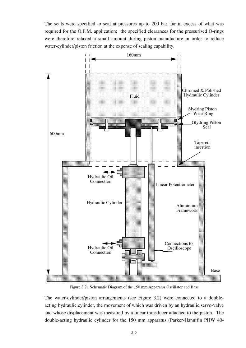
3:6
The seals were specified to seal at pressures up to 200 bar, far in excess of what was
required for the O.F.M. application: the specified clearances for the pressurised O-rings
were therefore relaxed a small amount during piston manufacture in order to reduce
water-cylinder/piston friction at the expense of sealing capability.
Hydraulic Oil Connection
Linear Potentiometer
Aluminium Framework
160mm
600mm
Chromed & Polished Hydraulic CylinderFluid
Hydraulic Cylinder
Hydraulic Oil Connection
Base
Tapered insertion
Glydring Piston Seal
Slydring Piston Wear Ring
Connections to Oscilloscope
Figure 3.2: Schematic Diagram of the 150 mm Apparatus Oscillator and Base
The water-cylinder/piston arrangements (see Figure 3.2) were connected to a double-
acting hydraulic cylinder, the movement of which was driven by an hydraulic servo-valve
and whose displacement was measured by a linear transducer attached to the piston. The
double-acting hydraulic cylinder for the 150 mm apparatus (Parker-Hannifin PHW 40-
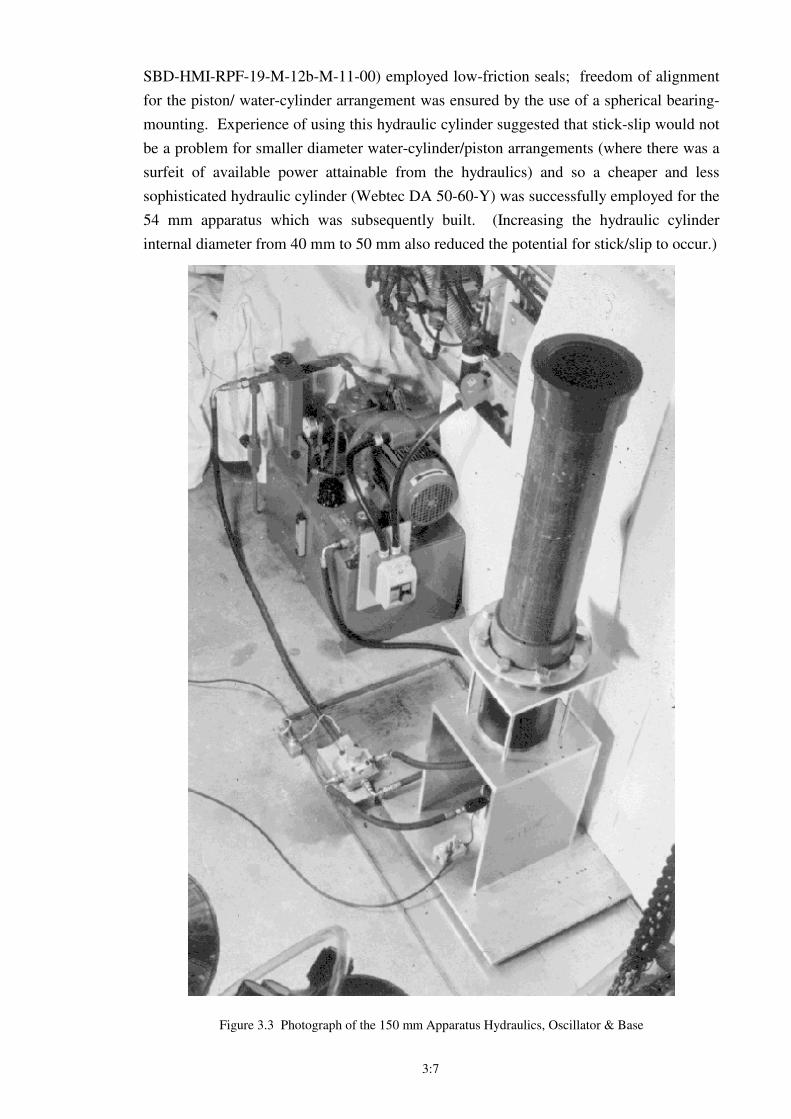
3:7
SBD-HMI-RPF-19-M-12b-M-11-00) employed low-friction seals; freedom of alignment
for the piston/ water-cylinder arrangement was ensured by the use of a spherical bearing-
mounting. Experience of using this hydraulic cylinder suggested that stick-slip would not
be a problem for smaller diameter water-cylinder/piston arrangements (where there was a
surfeit of available power attainable from the hydraulics) and so a cheaper and less
sophisticated hydraulic cylinder (Webtec DA 50-60-Y) was successfully employed for the
54 mm apparatus which was subsequently built. (Increasing the hydraulic cylinder
internal diameter from 40 mm to 50 mm also reduced the potential for stick/slip to occur.)
Figure 3.3 Photograph of the 150 mm Apparatus Hydraulics, Oscillator & Base
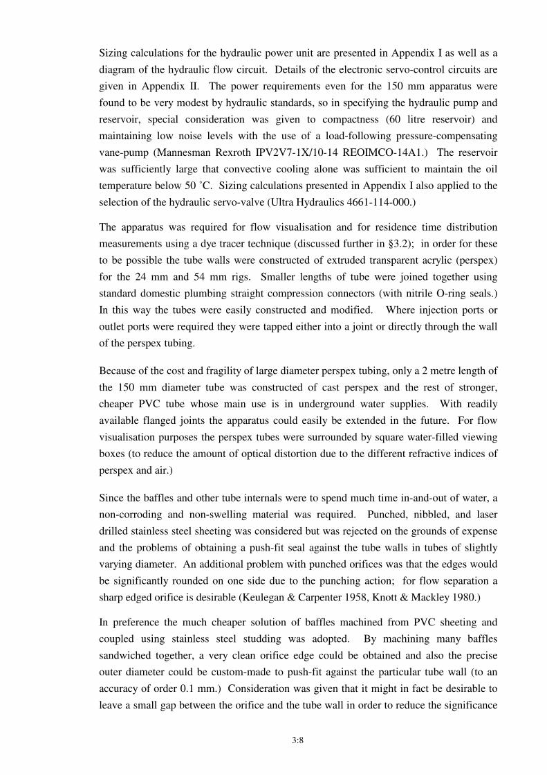
3:8
Sizing calculations for the hydraulic power unit are presented in Appendix I as well as a
diagram of the hydraulic flow circuit. Details of the electronic servo-control circuits are
given in Appendix II. The power requirements even for the 150 mm apparatus were
found to be very modest by hydraulic standards, so in specifying the hydraulic pump and
reservoir, special consideration was given to compactness (60 litre reservoir) and
maintaining low noise levels with the use of a load-following pressure-compensating
vane-pump (Mannesman Rexroth IPV2V7-1X/10-14 REOIMCO-14A1.) The reservoir
was sufficiently large that convective cooling alone was sufficient to maintain the oil
temperature below 50 ˚C. Sizing calculations presented in Appendix I also applied to the
selection of the hydraulic servo-valve (Ultra Hydraulics 4661-114-000.)
The apparatus was required for flow visualisation and for residence time distribution
measurements using a dye tracer technique (discussed further in §3.2); in order for these
to be possible the tube walls were constructed of extruded transparent acrylic (perspex)
for the 24 mm and 54 mm rigs. Smaller lengths of tube were joined together using
standard domestic plumbing straight compression connectors (with nitrile O-ring seals.)
In this way the tubes were easily constructed and modified. Where injection ports or
outlet ports were required they were tapped either into a joint or directly through the wall
of the perspex tubing.
Because of the cost and fragility of large diameter perspex tubing, only a 2 metre length of
the 150 mm diameter tube was constructed of cast perspex and the rest of stronger,
cheaper PVC tube whose main use is in underground water supplies. With readily
available flanged joints the apparatus could easily be extended in the future. For flow
visualisation purposes the perspex tubes were surrounded by square water-filled viewing
boxes (to reduce the amount of optical distortion due to the different refractive indices of
perspex and air.)
Since the baffles and other tube internals were to spend much time in-and-out of water, a
non-corroding and non-swelling material was required. Punched, nibbled, and laser
drilled stainless steel sheeting was considered but was rejected on the grounds of expense
and the problems of obtaining a push-fit seal against the tube walls in tubes of slightly
varying diameter. An additional problem with punched orifices was that the edges would
be significantly rounded on one side due to the punching action; for flow separation a
sharp edged orifice is desirable (Keulegan & Carpenter 1958, Knott & Mackley 1980.)
In preference the much cheaper solution of baffles machined from PVC sheeting and
coupled using stainless steel studding was adopted. By machining many baffles
sandwiched together, a very clean orifice edge could be obtained and also the precise
outer diameter could be custom-made to push-fit against the particular tube wall (to an
accuracy of order 0.1 mm.) Consideration was given that it might in fact be desirable to
leave a small gap between the orifice and the tube wall in order to reduce the significance
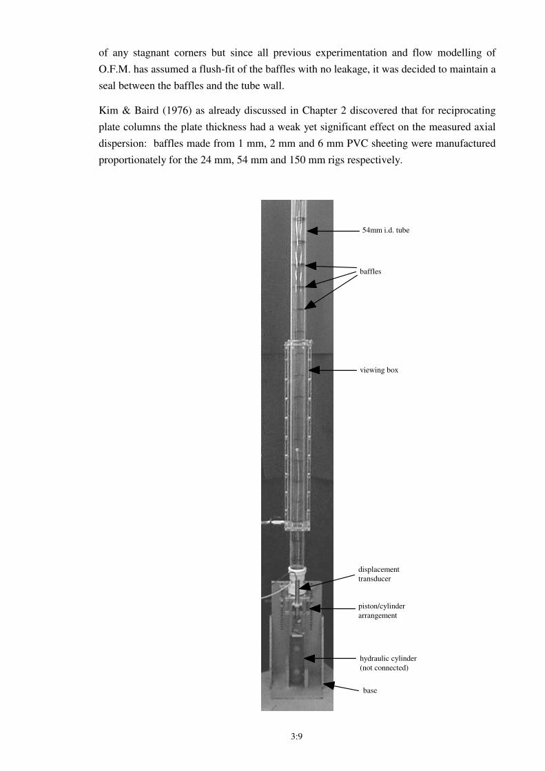
3:9
of any stagnant corners but since all previous experimentation and flow modelling of
O.F.M. has assumed a flush-fit of the baffles with no leakage, it was decided to maintain a
seal between the baffles and the tube wall.
Kim & Baird (1976) as already discussed in Chapter 2 discovered that for reciprocating
plate columns the plate thickness had a weak yet significant effect on the measured axial
dispersion: baffles made from 1 mm, 2 mm and 6 mm PVC sheeting were manufactured
proportionately for the 24 mm, 54 mm and 150 mm rigs respectively.
54mm i.d. tube
baffles
viewing box
piston/cylinder
arrangement
hydraulic cylinder
(not connected)
displacement
transducer
base
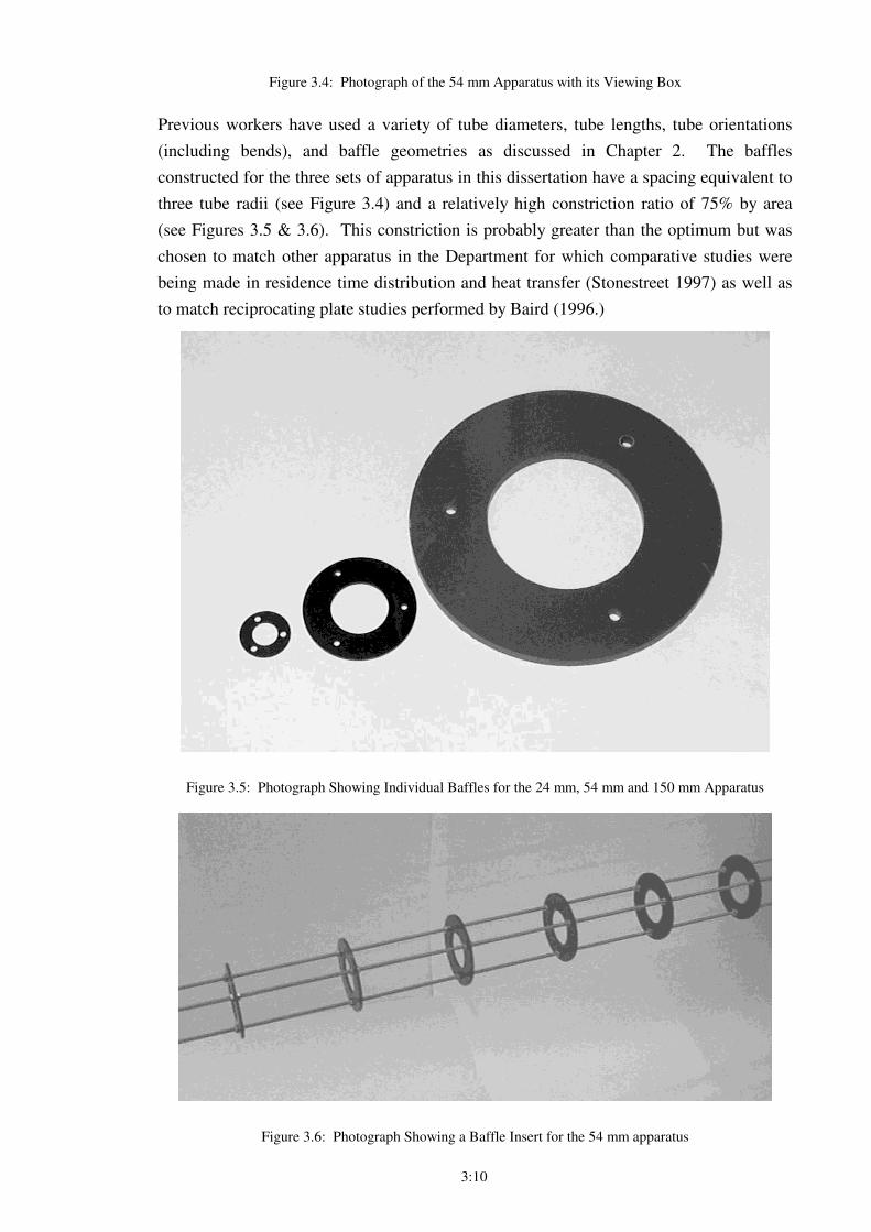
3:10
Figure 3.4: Photograph of the 54 mm Apparatus with its Viewing Box
Previous workers have used a variety of tube diameters, tube lengths, tube orientations
(including bends), and baffle geometries as discussed in Chapter 2. The baffles
constructed for the three sets of apparatus in this dissertation have a spacing equivalent to
three tube radii (see Figure 3.4) and a relatively high constriction ratio of 75% by area
(see Figures 3.5 & 3.6). This constriction is probably greater than the optimum but was
chosen to match other apparatus in the Department for which comparative studies were
being made in residence time distribution and heat transfer (Stonestreet 1997) as well as
to match reciprocating plate studies performed by Baird (1996.)
Figure 3.5: Photograph Showing Individual Baffles for the 24 mm, 54 mm and 150 mm Apparatus
Figure 3.6: Photograph Showing a Baffle Insert for the 54 mm apparatus
3:11
3.2 Experimental Methods
The two primary experimental methods reported in this thesis are imperfect pulse dye
tracer experiments (§3.2.1) and flow visualisation using fluorescent dye streaklines
(§3.2.2). Both methods have been taken from other areas of research and developed as
part of this thesis for use with Oscillatory Flow Mixing. Both sections begin with an
explanation of the choice of the experimental technique.
3.2.1 Imperfect Pulse Dye Tracer Experiments
All techniques for the measurement of axial dispersion involve some form of tracer
injection, whether a dye, salt solution, smoke or radioactive particles; the injection can be
a pulse or a continuous stream of tracer. A number of problems have been identified by
workers using salt-solutions and conductivity probes to measure axial dispersion and
these include inaccuracies due to density differences (Mackley & Ni 1993) and poor
averaging across the tube cross-section (Howes & Mackley 1990). The probes may also
affect the flow. Smoke is clearly inappropriate for a fluid system and the use of
radioactive particles is generally to be avoided where other methods exist, especially
when large quantities of (contaminated) liquid must be disposed of after each experiment.
An optical method of detecting a neutrally buoyant dye tracer was therefore selected. A
similar technique had already been used successfully for measuring concentrations of
suspended particles in O.F.M. (Mackley et al 1993) but not previously for measuring axial
dispersion. The optical technique has the advantages of not affecting the flow within the
tube and of being very cheap to construct compared to the purchase of commercial
conductivity probes, and can easily be located externally anywhere along the length of the
tube.
High power Light Emitting Diodes (up to 15,000 mcd power) were used to propagate a
beam of red light through the tube (wavelength approximately 660 nm). The intensity of
the transmitted light was measured by a photo diode that is sensitive to the same
wavelength. The photo diode allowed a current signal to pass proportional to the incident
light and this could be amplified and converted to a voltage signal (0-5 Volts) for data
recording. A blue dye tracer passing through the tube between the emitter and receiver
attenuated the light and hence the average concentration of dye could be calculated as
being proportional to the measured optical density. Details of the sensor calibration and
signal treatment are given in Appendix III.
The aim of the tracer experiments was firstly to ascertain the effectiveness of a chosen
model to describe the axial dispersion in the tube (due to net flow and oscillations) and
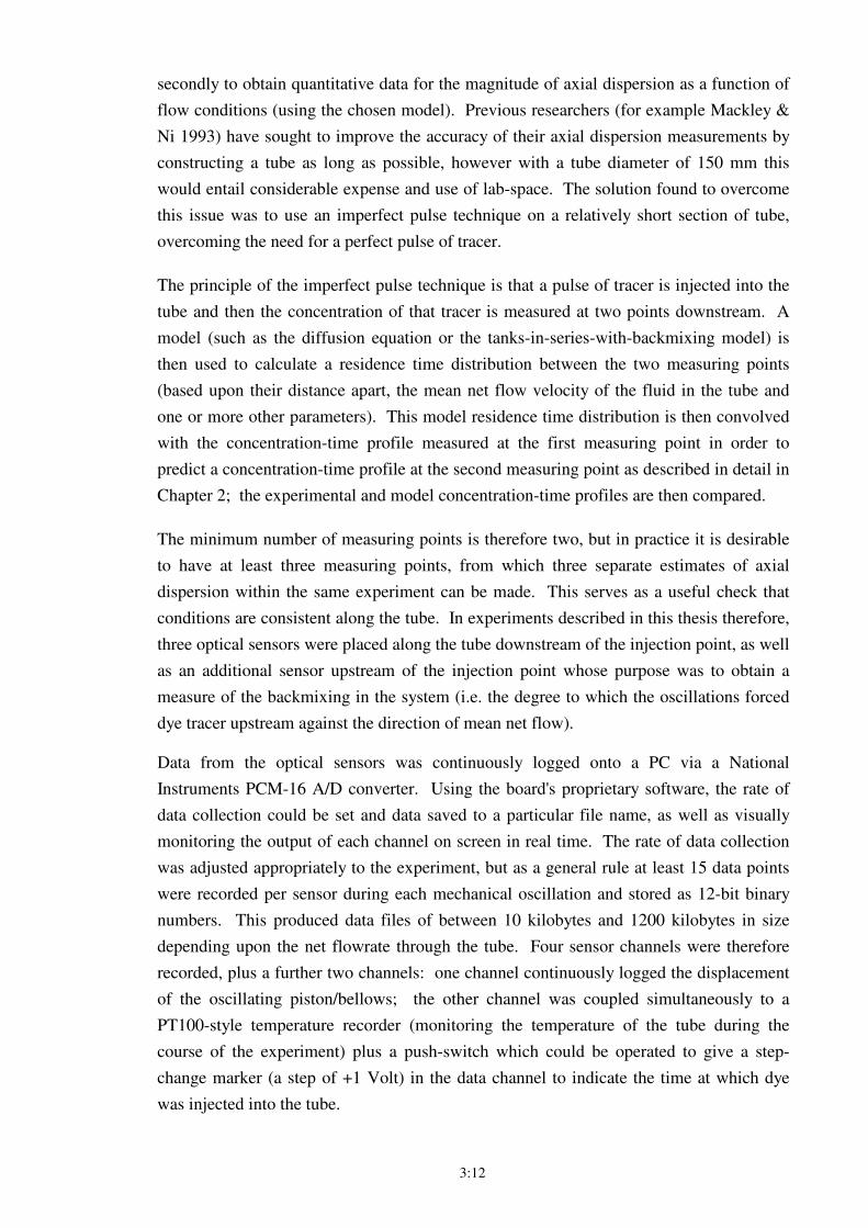
3:12
secondly to obtain quantitative data for the magnitude of axial dispersion as a function of
flow conditions (using the chosen model). Previous researchers (for example Mackley &
Ni 1993) have sought to improve the accuracy of their axial dispersion measurements by
constructing a tube as long as possible, however with a tube diameter of 150 mm this
would entail considerable expense and use of lab-space. The solution found to overcome
this issue was to use an imperfect pulse technique on a relatively short section of tube,
overcoming the need for a perfect pulse of tracer.
The principle of the imperfect pulse technique is that a pulse of tracer is injected into the
tube and then the concentration of that tracer is measured at two points downstream. A
model (such as the diffusion equation or the tanks-in-series-with-backmixing model) is
then used to calculate a residence time distribution between the two measuring points
(based upon their distance apart, the mean net flow velocity of the fluid in the tube and
one or more other parameters). This model residence time distribution is then convolved
with the concentration-time profile measured at the first measuring point in order to
predict a concentration-time profile at the second measuring point as described in detail in
Chapter 2; the experimental and model concentration-time profiles are then compared.
The minimum number of measuring points is therefore two, but in practice it is desirable
to have at least three measuring points, from which three separate estimates of axial
dispersion within the same experiment can be made. This serves as a useful check that
conditions are consistent along the tube. In experiments described in this thesis therefore,
three optical sensors were placed along the tube downstream of the injection point, as well
as an additional sensor upstream of the injection point whose purpose was to obtain a
measure of the backmixing in the system (i.e. the degree to which the oscillations forced
dye tracer upstream against the direction of mean net flow).
Data from the optical sensors was continuously logged onto a PC via a National
Instruments PCM-16 A/D converter. Using the board's proprietary software, the rate of
data collection could be set and data saved to a particular file name, as well as visually
monitoring the output of each channel on screen in real time. The rate of data collection
was adjusted appropriately to the experiment, but as a general rule at least 15 data points
were recorded per sensor during each mechanical oscillation and stored as 12-bit binary
numbers. This produced data files of between 10 kilobytes and 1200 kilobytes in size
depending upon the net flowrate through the tube. Four sensor channels were therefore
recorded, plus a further two channels: one channel continuously logged the displacement
of the oscillating piston/bellows; the other channel was coupled simultaneously to a
PT100-style temperature recorder (monitoring the temperature of the tube during the
course of the experiment) plus a push-switch which could be operated to give a step-
change marker (a step of +1 Volt) in the data channel to indicate the time at which dye
was injected into the tube.
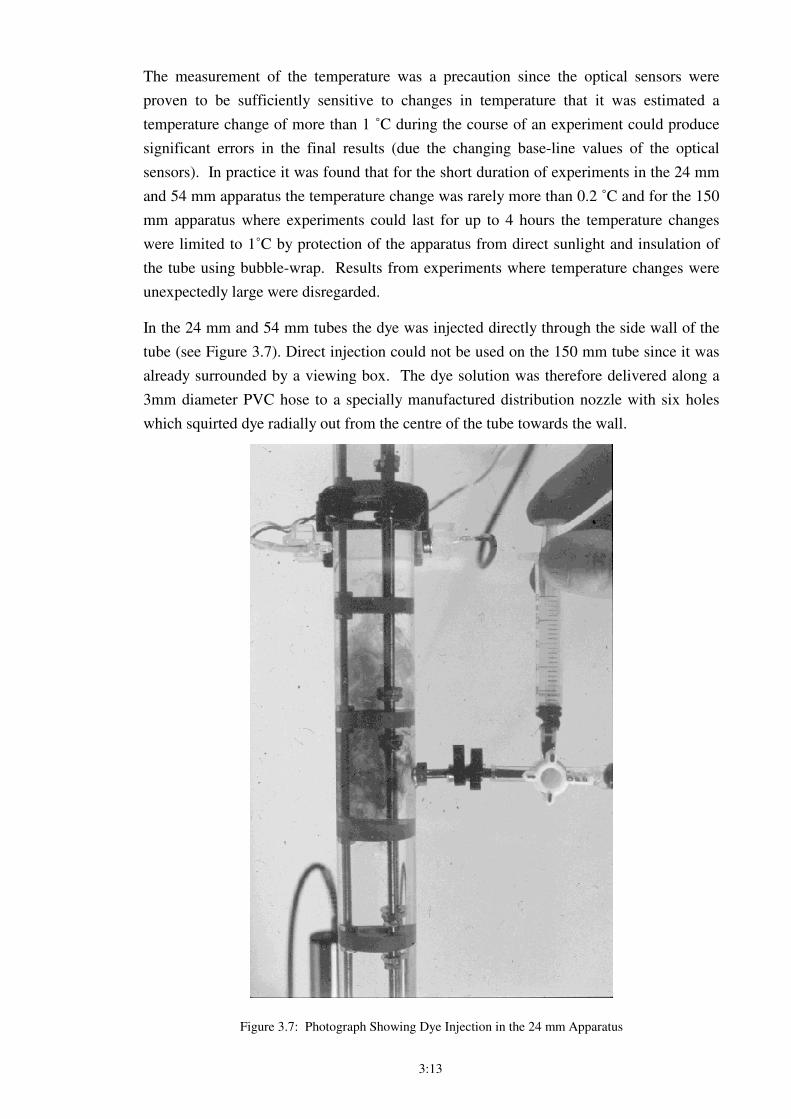
3:13
The measurement of the temperature was a precaution since the optical sensors were
proven to be sufficiently sensitive to changes in temperature that it was estimated a
temperature change of more than 1 ˚C during the course of an experiment could produce
significant errors in the final results (due the changing base-line values of the optical
sensors). In practice it was found that for the short duration of experiments in the 24 mm
and 54 mm apparatus the temperature change was rarely more than 0.2 ˚C and for the 150
mm apparatus where experiments could last for up to 4 hours the temperature changes
were limited to 1˚C by protection of the apparatus from direct sunlight and insulation of
the tube using bubble-wrap. Results from experiments where temperature changes were
unexpectedly large were disregarded.
In the 24 mm and 54 mm tubes the dye was injected directly through the side wall of the
tube (see Figure 3.7). Direct injection could not be used on the 150 mm tube since it was
already surrounded by a viewing box. The dye solution was therefore delivered along a
3mm diameter PVC hose to a specially manufactured distribution nozzle with six holes
which squirted dye radially out from the centre of the tube towards the wall.
Figure 3.7: Photograph Showing Dye Injection in the 24 mm Apparatus

3:14
A technique using two syringes and a three-way valve was developed whereby the dye
was injected and then followed by an injection of ordinary water in order to flush any dye
remaining in the side-port. This was necessary because of the relatively small volumes of
dye solution being injected compared to the volume of the side-port (the distance of tube
between the syringe and the tube wall.) Figure 3.8 shows a series of photographs of a
typical dye injection experiment with net flow and oscillation. The dye is injected close
to the base of the tube (Fig 3.8a) and moves up the tube in the direction of the net flow
(Fig 3.8b-f), dispersing as the experiment progresses. The apparatus is shown without the
optical sensors used to detect dye concentration.
(a) (b) (c) (d) (e) (f)
Figure 3.8: Photograph Showing a Typical Experiment in the 24 mm Apparatus
The dye selected was methylene blue because of its high optical density at low
concentrations: this allowed very dilute solutions to be used for which the very small
density difference between the dye solution and the bulk fluid in the tube was
insignificant over the time scale of most experiments. (The sensitivity of the optical
sensor technique also allowed very dilute concentrations of the dye to be measured, even
where not detectable by the human eye.)
The volume and quantity of dye injected did not scale proportionally to the volume of
fluid in the tube: this was due to the decreasing intensity of the L.E.D. beam of light
shining through the tube meaning that more dilute solutions had to be used for the larger
apparatus in order to maintain resolution (see Table 3.3). It was found that the results of
experiments were insensitive to the rate of dye injection; typically the dye was injected
over the course of approximately one oscillation.
3:15
Apparatus Volume of Dye Injected Concentration of Dye Injected
24 mm Apparatus 0.7 ml 0.0001 g/ml
54 mm Apparatus 2.5 ml 0.0001 g/ml
150 mm Apparatus 20 ml 0.0001 g/ml
Table 3.3: Typical Quantity of Dye Injected for Axial Dispersion Measurements
Particularly for the 150 mm apparatus, the technique was somewhat sensitive to the
presence of background light: all the apparatus were therefore shrouded in opaque black
paper surrounded with black plastic sheeting (bin-liners!) which effectively eliminated all
background light. The method could perhaps have been improved by using a stronger
beam light source such as a laser-pen, but the additional expense and potential safety
implications outweighed any possible advantage.
A typical experimental was conducted thus:
1. Net flowrate and oscillatory conditions were set and left for several minutes to
ensure that quasi-steady-state had been reached
2. The recording of data from the optical sensors (4 channels), oscillation
displacement (1 channel) and start/stop/temperature channel (1 channel) was
started and the base-levels for each channel recorded for at least 300 data points
per channel
4. The dye tracer was injected into the tube while the start/stop push switch was
pressed simultaneously to mark the start of the experiment
5. The experiment was allowed to run until the output from the optical sensors
readings had substantially returned to their base levels
6. Data recording was ceased and the collected data stored to a particular file name
7. The tube was thoroughly flushed to remove any residual dye before commencing
the next experiment
A critical aspect of the experiments was to maintain a constant net flowrate during the
course of the experiment: flowrates varied from 30 ml/min up to approximately 20 000
ml/min and had to be a smooth flow (otherwise any pulsation could have caused increased
flow separation in the tube). Peristaltic pumps were found to give an unsatisfactory
pulsating flow as well as having a limited range of operation. Instead, the flow was
regulated by a needle valve and monitored by a range of rotameters (selected according
the flowrate). This worked very successfully to give a steady flow, with the water supply
being delivered from header-tanks maintained at constant pressure. In each apparatus, the
3:16
net flow was delivered as close as possible to the base of the tube for continuous
operation, with a simple overflow arrangement at the top of the tube.
3.2.2 Flow Visualisation Using Fluorescent Dye Streaklines
A method of flow visualisation was required in order to understand better the types of
flow found in O.F.M., to examine the effect of tube diameter on the observed fluid
mechanics and to help interpret the trends in axial dispersion measurements. This was
particularly relevant to understanding of the behaviour of multi-orifice baffles described
in Chapter 8. Existing techniques such as seeding the flow with particles were inadequate
for flow visualisation in tubes of greatly differing diameter, so a novel technique was
sought. The required properties for the technique were that it would not affect the flow,
would faithfully follow the flow, and that it could be used on tubes of any diameter.
In previous studies of O.F.M. the principal method of flow visualisation used was the slit-
illumination of neutrally-buoyant 100 micron polyethylene particles suspended in the flow
and photographed using timed-exposures to create streaklines of the particle trajectories
(Brunold et al 1989). This method has a number of disadvantages: it does not show the
degree of mixing in the tube; it is best used in batch mode since for continuous flow the
particles will be washed out of the tube; the particles are difficult to handle and suspend
and may affect the flow itself; the particles may not faithfully follow the direction of flow
if they are not neutrally buoyant, and the particles are too small to be resolved in
photographs of larger tube diameters. The latter problem could in principle be overcome
by the use of larger diameter particles, but as their size increases to the order of mm then
it becomes more problematic to obtain neutrally buoyant particles and to minimise the
inertia of the particles.
Another method for observing flow patterns in O.F.M. is the simple injection of dye (such
as is already used in this thesis for the measurement of axial dispersion, also adopted by
Saraiva 1997). This technique was used in initial investigations of the flows examined in
this thesis but has very limited effectiveness since after only a few oscillations the dye is
well-distributed across the tube and no fine detail of the flow can be distinguished.
Particle Image Velocimetry (P.I.V.) and Laser Doppler Velocimetry (L.D.V.) are powerful
techniques which yield much information about the flow (Hayden 1997), but both are
very costly and time consuming to set up and were therefore impractical for use on three
separate rigs.
Flow visualisation using a fluorescent dye has previously been used by researchers in
different areas (for example static mixers, Reeder et al 1997). The technique typically
used a fanned laser-beam of about 1 mm width to illuminate a longitudinal-section
through the tube. Fluorescent dye was then injected into the flow and was illuminated
only when it passed through the fanned laser-beam, allowing a section through the flow to
be examined, photographed or videoed in detail. The resulting streakline flow
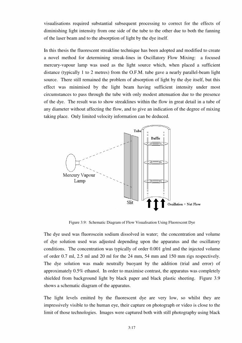
3:17
visualisations required substantial subsequent processing to correct for the effects of
diminishing light intensity from one side of the tube to the other due to both the fanning
of the laser beam and to the absorption of light by the dye itself.
In this thesis the fluorescent streakline technique has been adopted and modified to create
a novel method for determining streak-lines in Oscillatory Flow Mixing: a focused
mercury-vapour lamp was used as the light source which, when placed a sufficient
distance (typically 1 to 2 metres) from the O.F.M. tube gave a nearly parallel-beam light
source. There still remained the problem of absorption of light by the dye itself, but this
effect was minimised by the light beam having sufficient intensity under most
circumstances to pass through the tube with only modest attenuation due to the presence
of the dye. The result was to show streaklines within the flow in great detail in a tube of
any diameter without affecting the flow, and to give an indication of the degree of mixing
taking place. Only limited velocity information can be deduced.
Figure 3.9: Schematic Diagram of Flow Visualisation Using Fluorescent Dye
The dye used was fluoroscein sodium dissolved in water; the concentration and volume
of dye solution used was adjusted depending upon the apparatus and the oscillatory
conditions. The concentration was typically of order 0.001 g/ml and the injected volume
of order 0.7 ml, 2.5 ml and 20 ml for the 24 mm, 54 mm and 150 mm rigs respectively.
The dye solution was made neutrally buoyant by the addition (trial and error) of
approximately 0.5% ethanol. In order to maximise contrast, the apparatus was completely
shielded from background light by black paper and black plastic sheeting. Figure 3.9
shows a schematic diagram of the apparatus.
The light levels emitted by the fluorescent dye are very low, so whilst they are
impressively visible to the human eye, their capture on photograph or video is close to the
limit of those technologies. Images were captured both with still photography using black

3:18
& white high speed film up to ASA 6400 and a Super-VHS video camera with a fully-
open aperture.
4:1
4. Analysis of Results for Axial Dispersion
This chapter describes the treatment of the experimental raw data acquired for axial
dispersion measurements. In order to analyse the data an analysis programme was written
using Matlab code. Details of the programme code are given in Appendix IV, while §4.1
describes the algorithms used by the analysis programme to extract axial dispersion
measurements from the data. §4.2 gives an explanation of the correct form of the
imperfect pulse solution to the diffusion equation (for which conflicting solutions arise in
the literature, see Chapter 2). §4.3 is a case study analysis (Case Study 1) of a typical
imperfect pulse tracer experiment in the 24 mm apparatus. §4.4 is a case study analysis
(Case Study 2) of a typical tracer experiment with no net flow in the 150 mm apparatus.
4.1 Development of Axial Dispersion Analysis Programme in Matlab
Having recorded data from the four optical sensors and from the displacement transducer
monitoring the wave form of the oscillation as described in the preceding chapter, the raw
data was stored on a standard PC hard disc. In order to extract useful information, an
analysis programme was created in Matlab (a Windows-based commercial software
package) and used to manipulate the data. This section describes the algorithms used in
the analysis programme; at all stages of the development of the code it was rigorously
tested for reliability and self-consistency.
Matlab was chosen because of its efficiency at handling very large matrices of data (for
some experiments in excess of 600 000 data points). While this number of data points
may at first seem excessive, it must be remembered that in order to measure variations in
optical sensor output during one oscillation cycle, a substantial sampling-rate was
required; during the analysis, the data could be greatly compressed.
Programming in Matlab is quite similar to many other programming languages, except
that compiling is not necessary. Many smaller subroutines can be combined together to
form a larger programme, and this was the sequential structure chosen for the analysis
programme. The most up to date version of the analysis programme happened to be
version 7, and this consisted of two separate programmes named net7 and nonet7, both
of which shared mostly the same subroutines: net7 was used to analyse experiments
with a net flow (with or without oscillations - see Case Study 1), whilst nonet7 was used
to analyse experiments without a net flow (oscillation only - see Case Study 2). It was
necessary to make this distinction because while in experiments with a net flow the dye is
eventually washed out of the tube and the concentrations measured by the optical sensors
return to zero, in experiments with no net flow the dye remains in the tube and the
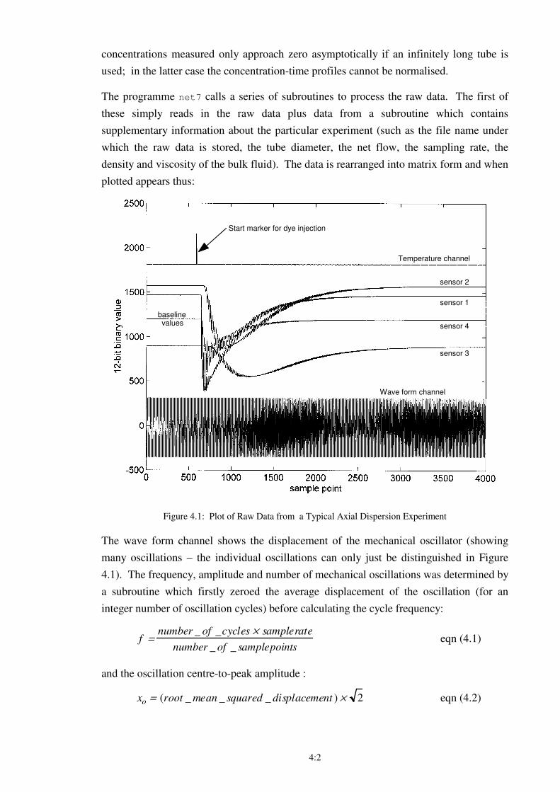
4:2
concentrations measured only approach zero asymptotically if an infinitely long tube is
used; in the latter case the concentration-time profiles cannot be normalised.
The programme net7 calls a series of subroutines to process the raw data. The first of
these simply reads in the raw data plus data from a subroutine which contains
supplementary information about the particular experiment (such as the file name under
which the raw data is stored, the tube diameter, the net flow, the sampling rate, the
density and viscosity of the bulk fluid). The data is rearranged into matrix form and when
plotted appears thus:
Temperature channel
Start marker for dye injection
Wave form channel
sensor 3
sensor 1
sensor 4
sensor 2
baselinevalues
Figure 4.1: Plot of Raw Data from a Typical Axial Dispersion Experiment
The wave form channel shows the displacement of the mechanical oscillator (showing
many oscillations – the individual oscillations can only just be distinguished in Figure
4.1). The frequency, amplitude and number of mechanical oscillations was determined by
a subroutine which firstly zeroed the average displacement of the oscillation (for an
integer number of oscillation cycles) before calculating the cycle frequency:
f =
number _ of _cycles × samplerate
number _ of _ samplepoints eqn (4.1)
and the oscillation centre-to-peak amplitude :
xo = (root _ mean _ squared _ displacement ) × 2 eqn (4.2)
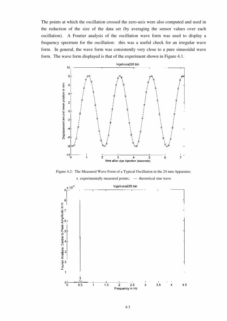
4:3
The points at which the oscillation crossed the zero-axis were also computed and used in
the reduction of the size of the data set (by averaging the sensor values over each
oscillation). A Fourier analysis of the oscillation wave form was used to display a
frequency spectrum for the oscillation: this was a useful check for an irregular wave
form. In general, the wave form was consistently very close to a pure sinusoidal wave
form. The wave form displayed is that of the experiment shown in Figure 4.1.
Figure 4.2: The Measured Wave Form of a Typical Oscillation in the 24 mm Apparatus:
x experimentally measured points; --- theoretical sine wave
4:4
Figure 4.3: Frequency Spectrum of a Typical Oscillation in the 24 mm Apparatus
The start marker of the experiment (the moment of dye injection) is clearly visible in
Figure 4.1 as a pulse in the temperature/timing channel; the experiment was stopped
sometime after all the dye had exited the baffled tube. Several subroutines in the analysis
programme are dedicated to detecting the start marker recorded on the timing/temperature
channel and to removing all data points from before the start of the dye injection. An
additional subroutine also records the baseline levels of the optical sensors before the start
of the dye injection.
Those baseline values are then used to convert the optical sensor output voltages into
optical density measurements: since log
Io
I∝ concentration where Io is the baseline
intensity and I is the experimental intensity, the optical sensor output voltages can be
converted into absolute concentrations (see Appendix III). These values, after correction
by a previously determined sensor calibration, represent the average concentration of dye
along the path of the transmitted light for each optical sensor.
For simplicity, these concentrations are then normalised so that for example ′ C 2 and ′ C 1
are the normalised experimental concentrations at optical sensors 2 and 1 respectively:
′ C 2(t ) =C2 (t )
C2( t )dt
0
∞
∫ and
′ C 1( t ) =C1(t )
C1( t )dt
0
∞
∫ eqns (4.3 & 4.4)
This is not applicable to the single optical sensor located upstream of the dye injection
point, to which a conversion factor is applied which is the average of that of the other
optical sensors'. This introduces a small error (<5%) into the values for the upstream
sensor. The normalisation is not strictly necessary, but allows the results to be
conveniently scaled onto a single axes for comparisons to be made. In the case of
experiments without net flow, the normalisation procedure cannot be applied and
therefore the data is retained as a concentration in mg/l.
The value of the mean net flow velocity U is calculable directly from the net volumetric
flow rate Q, the distance between the probes L and the volume of fluid between probes V:
U =
QL
V eqn (4.5)
A second method for calculating U is to calculate the difference in time between the first
moments of area of the concentration profiles and which should be in good agreement
with that given by the previous equation.
U =L
t ′ C 2 (t )dt − t ′ C 1(t )dt
0
∞
∫0
∞
∫ eqn (4.6)
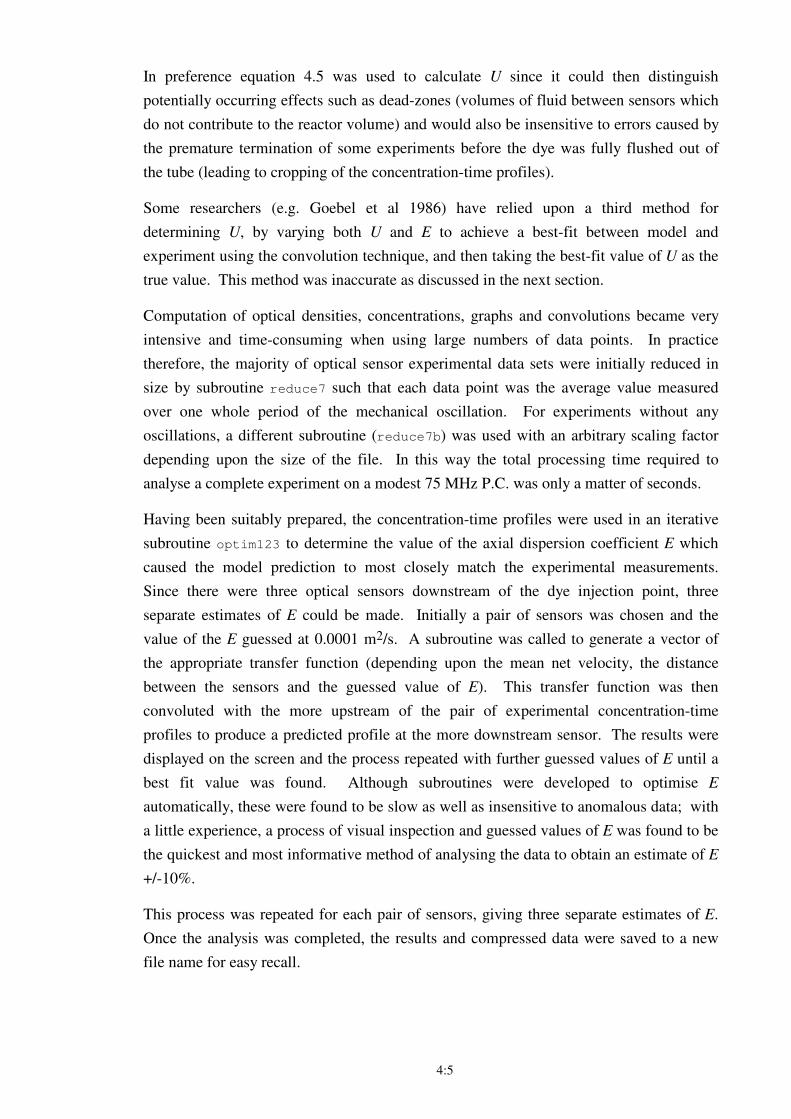
4:5
In preference equation 4.5 was used to calculate U since it could then distinguish
potentially occurring effects such as dead-zones (volumes of fluid between sensors which
do not contribute to the reactor volume) and would also be insensitive to errors caused by
the premature termination of some experiments before the dye was fully flushed out of
the tube (leading to cropping of the concentration-time profiles).
Some researchers (e.g. Goebel et al 1986) have relied upon a third method for
determining U, by varying both U and E to achieve a best-fit between model and
experiment using the convolution technique, and then taking the best-fit value of U as the
true value. This method was inaccurate as discussed in the next section.
Computation of optical densities, concentrations, graphs and convolutions became very
intensive and time-consuming when using large numbers of data points. In practice
therefore, the majority of optical sensor experimental data sets were initially reduced in
size by subroutine reduce7 such that each data point was the average value measured
over one whole period of the mechanical oscillation. For experiments without any
oscillations, a different subroutine (reduce7b) was used with an arbitrary scaling factor
depending upon the size of the file. In this way the total processing time required to
analyse a complete experiment on a modest 75 MHz P.C. was only a matter of seconds.
Having been suitably prepared, the concentration-time profiles were used in an iterative
subroutine optim123 to determine the value of the axial dispersion coefficient E which
caused the model prediction to most closely match the experimental measurements.
Since there were three optical sensors downstream of the dye injection point, three
separate estimates of E could be made. Initially a pair of sensors was chosen and the
value of the E guessed at 0.0001 m2/s. A subroutine was called to generate a vector of
the appropriate transfer function (depending upon the mean net velocity, the distance
between the sensors and the guessed value of E). This transfer function was then
convoluted with the more upstream of the pair of experimental concentration-time
profiles to produce a predicted profile at the more downstream sensor. The results were
displayed on the screen and the process repeated with further guessed values of E until a
best fit value was found. Although subroutines were developed to optimise E
automatically, these were found to be slow as well as insensitive to anomalous data; with
a little experience, a process of visual inspection and guessed values of E was found to be
the quickest and most informative method of analysing the data to obtain an estimate of E
+/-10%.
This process was repeated for each pair of sensors, giving three separate estimates of E.
Once the analysis was completed, the results and compressed data were saved to a new
file name for easy recall.
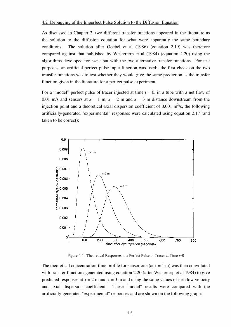
4:6
4.2 Debugging of the Imperfect Pulse Solution to the Diffusion Equation
As discussed in Chapter 2, two different transfer functions appeared in the literature as
the solution to the diffusion equation for what were apparently the same boundary
conditions. The solution after Goebel et al (1986) (equation 2.19) was therefore
compared against that published by Westerterp et al (1984) (equation 2.20) using the
algorithms developed for net7 but with the two alternative transfer functions. For test
purposes, an artificial perfect pulse input function was used; the first check on the two
transfer functions was to test whether they would give the same prediction as the transfer
function given in the literature for a perfect pulse experiment.
For a “model” perfect pulse of tracer injected at time t = 0, in a tube with a net flow of
0.01 m/s and sensors at x = 1 m, x = 2 m and x = 3 m distance downstream from the
injection point and a theoretical axial dispersion coefficient of 0.001 m2/s, the following
artificially-generated "experimental" responses were calculated using equation 2.17 (and
taken to be correct):
x=1 m
x=2 m
x=3 m
Figure 4.4: Theoretical Responses to a Perfect Pulse of Tracer at Time t=0
The theoretical concentration-time profile for sensor one (at x = 1 m) was then convoluted
with transfer functions generated using equation 2.20 (after Westerterp et al 1984) to give
predicted responses at x = 2 m and x = 3 m and using the same values of net flow velocity
and axial dispersion coefficient. These "model" results were compared with the
artificially-generated "experimental" responses and are shown on the following graph:
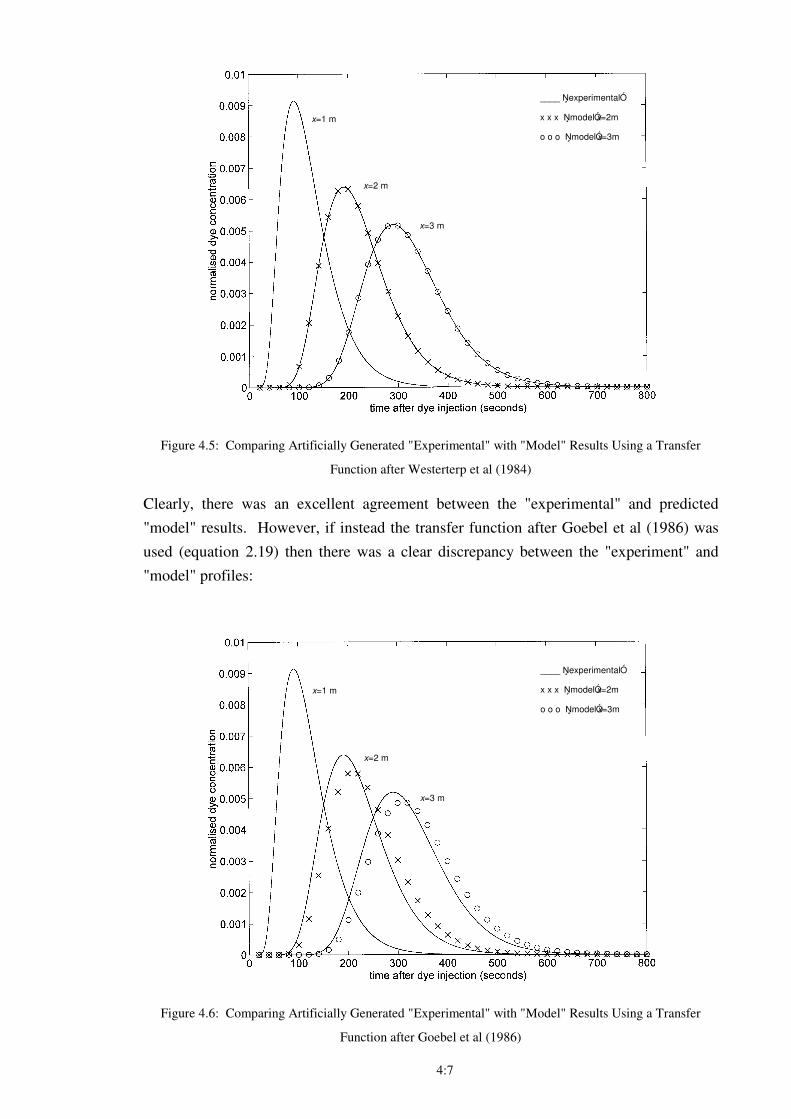
4:7
x=1 m
x=2 m
x=3 m
____ ŅexperimentalÓx x x ŅmodelÓ x=2mo o o ŅmodelÓ x=3m
Figure 4.5: Comparing Artificially Generated "Experimental" with "Model" Results Using a Transfer
Function after Westerterp et al (1984)
Clearly, there was an excellent agreement between the "experimental" and predicted
"model" results. However, if instead the transfer function after Goebel et al (1986) was
used (equation 2.19) then there was a clear discrepancy between the "experiment" and
"model" profiles:
x=1 m
x=2 m
x=3 m
____ ŅexperimentalÓx x x ŅmodelÓ x=2mo o o ŅmodelÓ x=3m
Figure 4.6: Comparing Artificially Generated "Experimental" with "Model" Results Using a Transfer
Function after Goebel et al (1986)
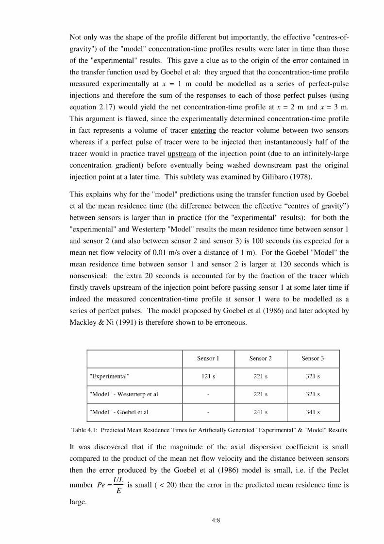
4:8
Not only was the shape of the profile different but importantly, the effective "centres-of-
gravity") of the "model" concentration-time profiles results were later in time than those
of the "experimental" results. This gave a clue as to the origin of the error contained in
the transfer function used by Goebel et al: they argued that the concentration-time profile
measured experimentally at x = 1 m could be modelled as a series of perfect-pulse
injections and therefore the sum of the responses to each of those perfect pulses (using
equation 2.17) would yield the net concentration-time profile at x = 2 m and x = 3 m.
This argument is flawed, since the experimentally determined concentration-time profile
in fact represents a volume of tracer entering the reactor volume between two sensors
whereas if a perfect pulse of tracer were to be injected then instantaneously half of the
tracer would in practice travel upstream of the injection point (due to an infinitely-large
concentration gradient) before eventually being washed downstream past the original
injection point at a later time. This subtlety was examined by Gilibaro (1978).
This explains why for the "model" predictions using the transfer function used by Goebel
et al the mean residence time (the difference between the effective “centres of gravity”)
between sensors is larger than in practice (for the "experimental" results): for both the
"experimental" and Westerterp "Model" results the mean residence time between sensor 1
and sensor 2 (and also between sensor 2 and sensor 3) is 100 seconds (as expected for a
mean net flow velocity of 0.01 m/s over a distance of 1 m). For the Goebel "Model" the
mean residence time between sensor 1 and sensor 2 is larger at 120 seconds which is
nonsensical: the extra 20 seconds is accounted for by the fraction of the tracer which
firstly travels upstream of the injection point before passing sensor 1 at some later time if
indeed the measured concentration-time profile at sensor 1 were to be modelled as a
series of perfect pulses. The model proposed by Goebel et al (1986) and later adopted by
Mackley & Ni (1991) is therefore shown to be erroneous.
Sensor 1 Sensor 2 Sensor 3
"Experimental" 121 s 221 s 321 s
"Model" - Westerterp et al - 221 s 321 s
"Model" - Goebel et al - 241 s 341 s
Table 4.1: Predicted Mean Residence Times for Artificially Generated "Experimental" & "Model" Results
It was discovered that if the magnitude of the axial dispersion coefficient is small
compared to the product of the mean net flow velocity and the distance between sensors
then the error produced by the Goebel et al (1986) model is small, i.e. if the Peclet
number Pe =
UL
E is small ( < 20) then the error in the predicted mean residence time is
large.
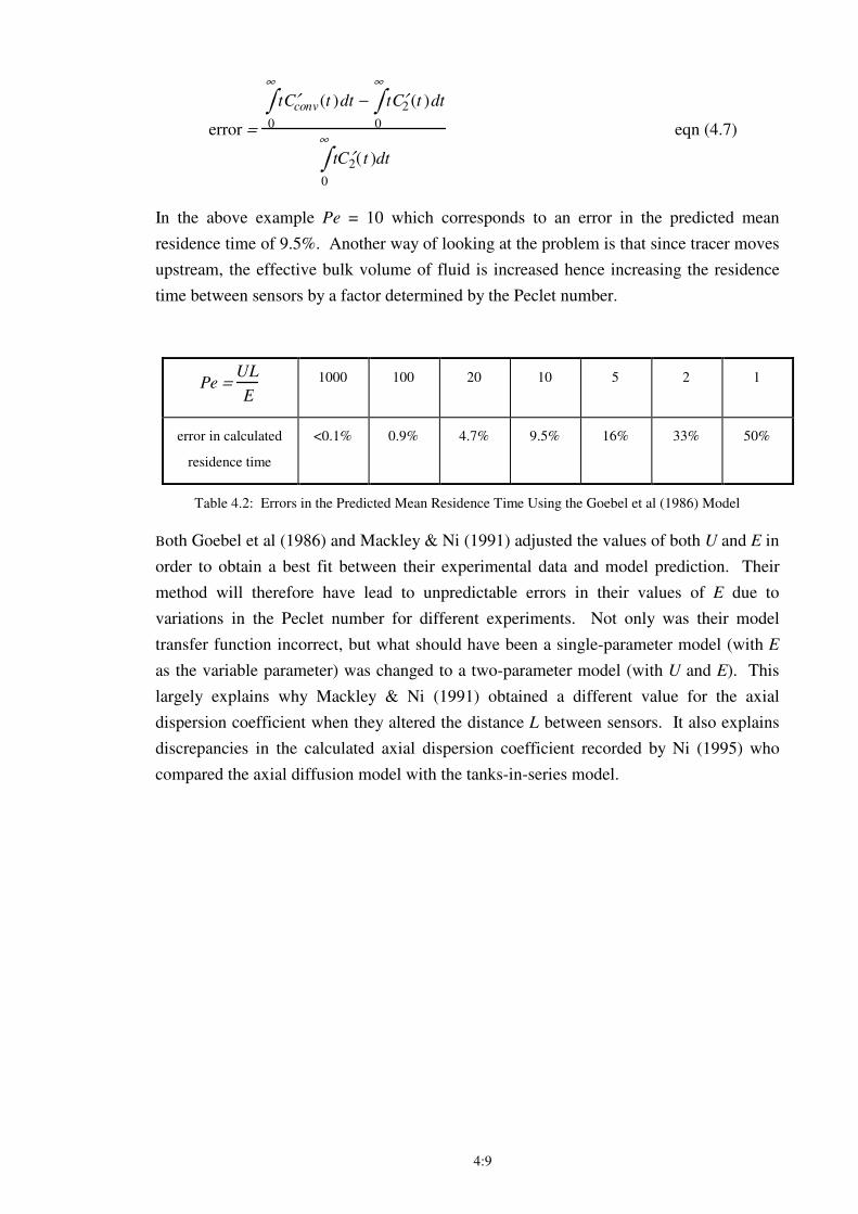
4:9
error =
t ′ C conv(t )dt
0
∞
∫ − t ′ C 2 (t )dt
0
∞
∫
t ′ C 2( t )dt
0
∞
∫ eqn (4.7)
In the above example Pe = 10 which corresponds to an error in the predicted mean
residence time of 9.5%. Another way of looking at the problem is that since tracer moves
upstream, the effective bulk volume of fluid is increased hence increasing the residence
time between sensors by a factor determined by the Peclet number.
Pe =
UL
E 1000 100 20 10 5 2 1
error in calculated
residence time
<0.1% 0.9% 4.7% 9.5% 16% 33% 50%
Table 4.2: Errors in the Predicted Mean Residence Time Using the Goebel et al (1986) Model
Both Goebel et al (1986) and Mackley & Ni (1991) adjusted the values of both U and E in
order to obtain a best fit between their experimental data and model prediction. Their
method will therefore have lead to unpredictable errors in their values of E due to
variations in the Peclet number for different experiments. Not only was their model
transfer function incorrect, but what should have been a single-parameter model (with E
as the variable parameter) was changed to a two-parameter model (with U and E). This
largely explains why Mackley & Ni (1991) obtained a different value for the axial
dispersion coefficient when they altered the distance L between sensors. It also explains
discrepancies in the calculated axial dispersion coefficient recorded by Ni (1995) who
compared the axial diffusion model with the tanks-in-series model.
4:10
4.3 Case Study 1 - Analysis of a Typical Imperfect Pulse Tracer Experiment
The data shown in Figure 4.1 is typical of an experiment in the 24 mm baffled tube. The
mean net flow velocity was 116 ml/min with an oscillation frequency of 0.5 Hz and a
centre-to-peak amplitude of approximately 8.2 mm. The sample rate per channel was
50/6 Hz. The temperature of the apparatus at the start and finish of the experiment varied
only by 0.1 ˚C, so errors due to changing temperature during the experiment were treated
as negligible.
After processing of the raw data, the concentration-time profiles of the four optical
sensors (three downstream and one upstream of the injection point) were found to be:
sensor 1
sensor 3
sensor 2
sensor 4 (upstream)
Figure 4.7: Case Study 1 : Concentration-Time Profiles for the Optical Sensors
Note that the area under the concentration-time profile for the upstream sensor was
measured to be about 34% of that for the other sensors, a measure of the degree of
backmixing (axial dispersion of the dye against the direction of net flow) and which is
discussed further in Chapter 5. Note also that the profiles are significantly smoother than
in the original raw data: this is because the data points were averaged over one whole
oscillatory cycle (§4.1). The discrepancy in the total area under the concentration-time
profiles for sensors 2 and 3 compared to sensor 1 was 2.1% and 2.8% before
normalisation. This is a relatively small discrepancy within the expected experimental
error for the optical sensors; it supports the observation that effectively all the dye had
been successfully flushed through the tube.
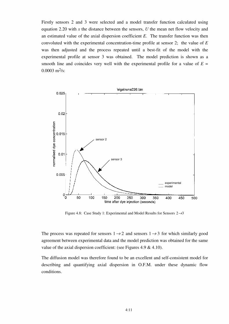
4:11
Firstly sensors 2 and 3 were selected and a model transfer function calculated using
equation 2.20 with x the distance between the sensors, U the mean net flow velocity and
an estimated value of the axial dispersion coefficient E. The transfer function was then
convoluted with the experimental concentration-time profile at sensor 2; the value of E
was then adjusted and the process repeated until a best-fit of the model with the
experimental profile at sensor 3 was obtained. The model prediction is shown as a
smooth line and coincides very well with the experimental profile for a value of E =
0.0003 m2/s:
sensor 2
sensor 3
___ experimental ...... model
Figure 4.8: Case Study 1: Experimental and Model Results for Sensors 2→3
The process was repeated for sensors 1→ 2 and sensors 1→ 3 for which similarly good
agreement between experimental data and the model prediction was obtained for the same
value of the axial dispersion coefficient: (see Figures 4.9 & 4.10).
The diffusion model was therefore found to be an excellent and self-consistent model for
describing and quantifying axial dispersion in O.F.M. under these dynamic flow
conditions.
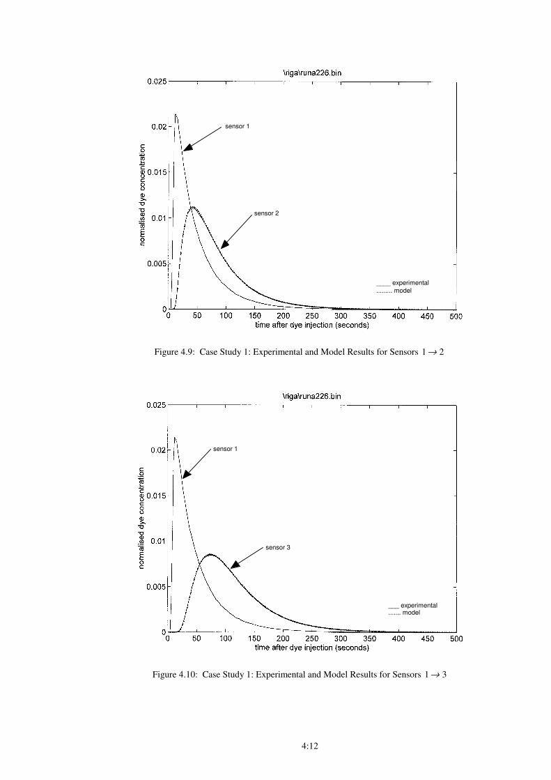
4:12
sensor 1
sensor 2
____ experimental ......... model
Figure 4.9: Case Study 1: Experimental and Model Results for Sensors 1→ 2
sensor 1
sensor 3
___ experimental....... model
Figure 4.10: Case Study 1: Experimental and Model Results for Sensors 1→ 3
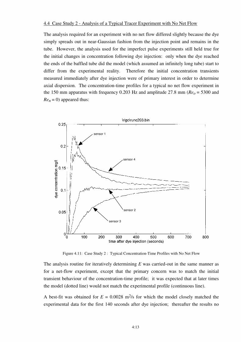
4:13
4.4 Case Study 2 - Analysis of a Typical Tracer Experiment with No Net Flow
The analysis required for an experiment with no net flow differed slightly because the dye
simply spreads out in near-Gaussian fashion from the injection point and remains in the
tube. However, the analysis used for the imperfect pulse experiments still held true for
the initial changes in concentration following dye injection: only when the dye reached
the ends of the baffled tube did the model (which assumed an infinitely long tube) start to
differ from the experimental reality. Therefore the initial concentration transients
measured immediately after dye injection were of primary interest in order to determine
axial dispersion. The concentration-time profiles for a typical no net flow experiment in
the 150 mm apparatus with frequency 0.203 Hz and amplitude 27.8 mm (Reo = 5300 and
Ren = 0) appeared thus:
sensor 1
sensor 4
sensor 2
sensor 3
Figure 4.11: Case Study 2 : Typical Concentration-Time Profiles with No Net Flow
The analysis routine for iteratively determining E was carried-out in the same manner as
for a net-flow experiment, except that the primary concern was to match the initial
transient behaviour of the concentration-time profile; it was expected that at later times
the model (dotted line) would not match the experimental profile (continuous line).
A best-fit was obtained for E = 0.0028 m2/s for which the model closely matched the
experimental data for the first 140 seconds after dye injection; thereafter the results no
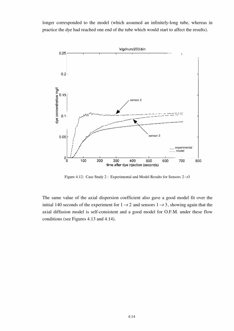
4:14
longer corresponded to the model (which assumed an infinitely-long tube, whereas in
practice the dye had reached one end of the tube which would start to affect the results).
___ experimental....... model
sensor 2
sensor 3
Figure 4.12: Case Study 2 : Experimental and Model Results for Sensors 2→3
The same value of the axial dispersion coefficient also gave a good model fit over the
initial 140 seconds of the experiment for 1→ 2 and sensors 1→ 3 , showing again that the
axial diffusion model is self-consistent and a good model for O.F.M. under these flow
conditions (see Figures 4.13 and 4.14).
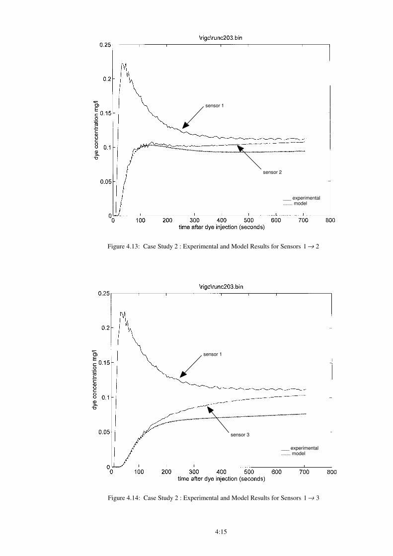
4:15
___ experimental....... model
sensor 1
sensor 2
Figure 4.13: Case Study 2 : Experimental and Model Results for Sensors 1→ 2
___ experimental....... model
sensor 1
sensor 3
Figure 4.14: Case Study 2 : Experimental and Model Results for Sensors 1→ 3
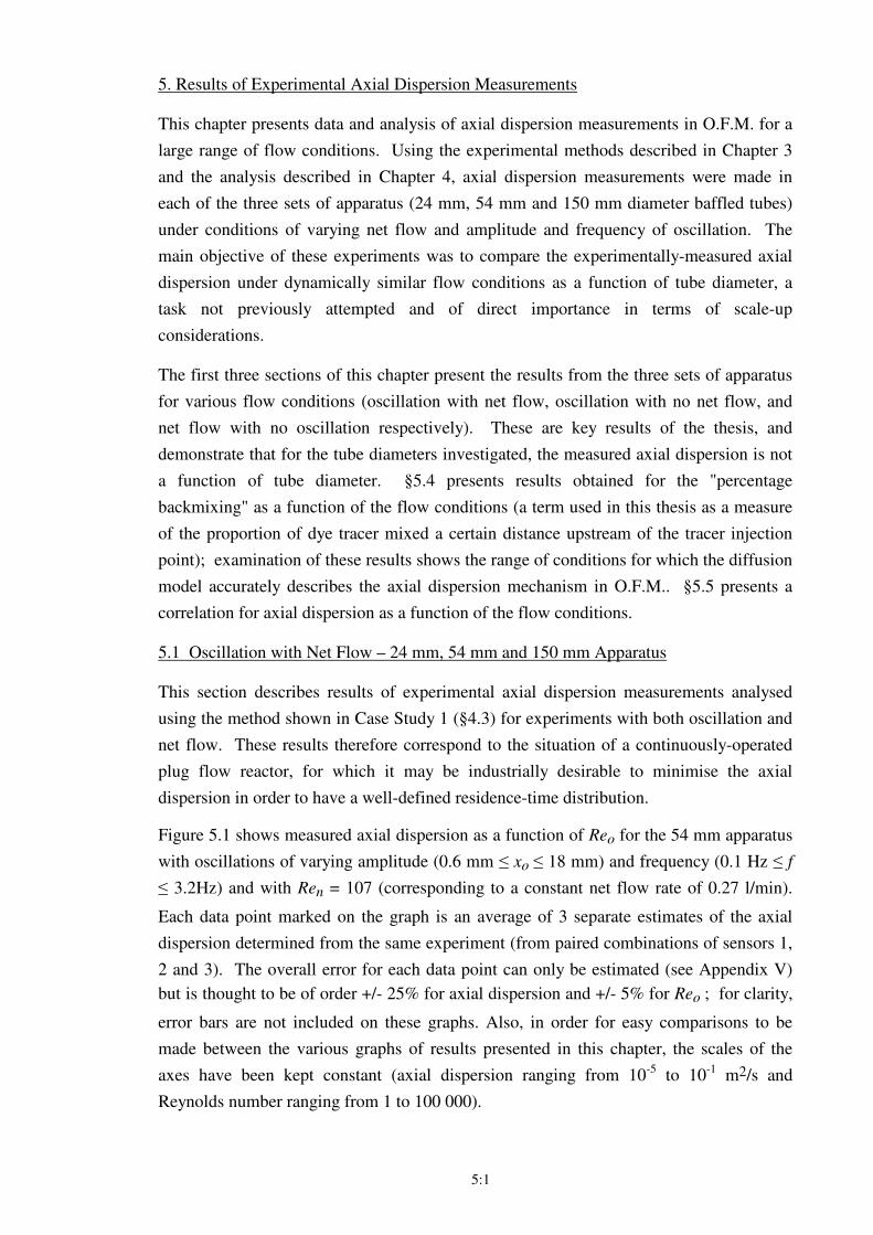
5:1
5. Results of Experimental Axial Dispersion Measurements
This chapter presents data and analysis of axial dispersion measurements in O.F.M. for a
large range of flow conditions. Using the experimental methods described in Chapter 3
and the analysis described in Chapter 4, axial dispersion measurements were made in
each of the three sets of apparatus (24 mm, 54 mm and 150 mm diameter baffled tubes)
under conditions of varying net flow and amplitude and frequency of oscillation. The
main objective of these experiments was to compare the experimentally-measured axial
dispersion under dynamically similar flow conditions as a function of tube diameter, a
task not previously attempted and of direct importance in terms of scale-up
considerations.
The first three sections of this chapter present the results from the three sets of apparatus
for various flow conditions (oscillation with net flow, oscillation with no net flow, and
net flow with no oscillation respectively). These are key results of the thesis, and
demonstrate that for the tube diameters investigated, the measured axial dispersion is not
a function of tube diameter. §5.4 presents results obtained for the "percentage
backmixing" as a function of the flow conditions (a term used in this thesis as a measure
of the proportion of dye tracer mixed a certain distance upstream of the tracer injection
point); examination of these results shows the range of conditions for which the diffusion
model accurately describes the axial dispersion mechanism in O.F.M.. §5.5 presents a
correlation for axial dispersion as a function of the flow conditions.
5.1 Oscillation with Net Flow – 24 mm, 54 mm and 150 mm Apparatus
This section describes results of experimental axial dispersion measurements analysed
using the method shown in Case Study 1 (§4.3) for experiments with both oscillation and
net flow. These results therefore correspond to the situation of a continuously-operated
plug flow reactor, for which it may be industrially desirable to minimise the axial
dispersion in order to have a well-defined residence-time distribution.
Figure 5.1 shows measured axial dispersion as a function of Reo for the 54 mm apparatus
with oscillations of varying amplitude (0.6 mm ≤ xo ≤ 18 mm) and frequency (0.1 Hz ≤ f
≤ 3.2Hz) and with Ren = 107 (corresponding to a constant net flow rate of 0.27 l/min).
Each data point marked on the graph is an average of 3 separate estimates of the axial
dispersion determined from the same experiment (from paired combinations of sensors 1,
2 and 3). The overall error for each data point can only be estimated (see Appendix V)
but is thought to be of order +/- 25% for axial dispersion and +/- 5% for Reo ; for clarity,
error bars are not included on these graphs. Also, in order for easy comparisons to be
made between the various graphs of results presented in this chapter, the scales of the
axes have been kept constant (axial dispersion ranging from 10-5
to 10-1
m2/s and
Reynolds number ranging from 1 to 100 000).
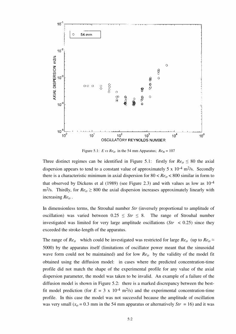
5:2
Figure 5.1: E vs Reo in the 54 mm Apparatus; Ren = 107
Three distinct regimes can be identified in Figure 5.1: firstly for Reo ≤ 80 the axial
dispersion appears to tend to a constant value of approximately 5 x 10⁻⁴ m2/s. Secondly
there is a characteristic minimum in axial dispersion for 80 < Reo < 800 similar in form to
that observed by Dickens et al (1989) (see Figure 2.3) and with values as low as 10-4
m2/s. Thirdly, for Reo ≥ 800 the axial dispersion increases approximately linearly with
increasing Reo .
In dimensionless terms, the Strouhal number Str (inversely proportional to amplitude of
oscillation) was varied between 0.25 ≤ Str ≤ 8. The range of Strouhal number
investigated was limited for very large amplitude oscillations (Str < 0.25) since they
exceeded the stroke-length of the apparatus.
The range of Reo which could be investigated was restricted for large Reo (up to Reo ≈
5000) by the apparatus itself (limitations of oscillator power meant that the sinusoidal
wave form could not be maintained) and for low Reo by the validity of the model fit
obtained using the diffusion model: in cases where the predicted concentration-time
profile did not match the shape of the experimental profile for any value of the axial
dispersion parameter, the model was taken to be invalid. An example of a failure of the
diffusion model is shown in Figure 5.2: there is a marked discrepancy between the best-
fit model prediction (for E = 3 x 10⁻⁴ m2/s) and the experimental concentration-time
profile. In this case the model was not successful because the amplitude of oscillation
was very small (xo = 0.3 mm in the 54 mm apparatus or alternatively Str = 16) and it was
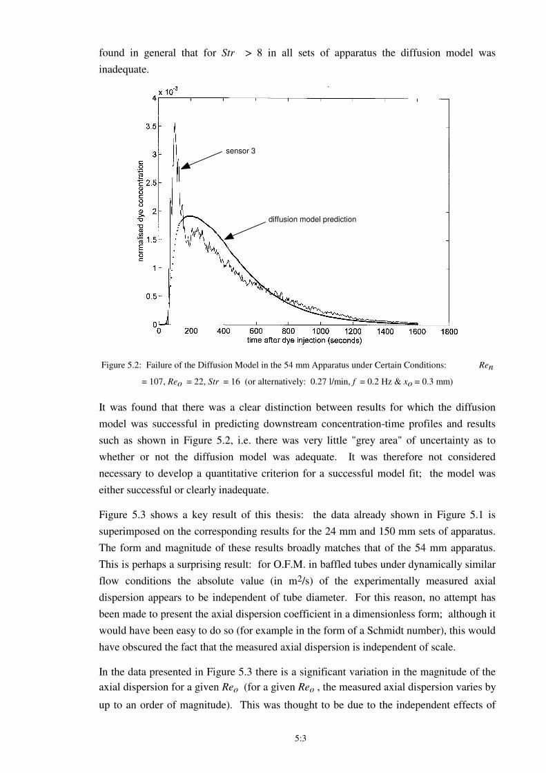
5:3
found in general that for Str > 8 in all sets of apparatus the diffusion model was
inadequate.
sensor 3
diffusion model prediction
Figure 5.2: Failure of the Diffusion Model in the 54 mm Apparatus under Certain Conditions: Ren
= 107, Reo = 22, Str = 16 (or alternatively: 0.27 l/min, f = 0.2 Hz & xo = 0.3 mm)
It was found that there was a clear distinction between results for which the diffusion
model was successful in predicting downstream concentration-time profiles and results
such as shown in Figure 5.2, i.e. there was very little "grey area" of uncertainty as to
whether or not the diffusion model was adequate. It was therefore not considered
necessary to develop a quantitative criterion for a successful model fit; the model was
either successful or clearly inadequate.
Figure 5.3 shows a key result of this thesis: the data already shown in Figure 5.1 is
superimposed on the corresponding results for the 24 mm and 150 mm sets of apparatus.
The form and magnitude of these results broadly matches that of the 54 mm apparatus.
This is perhaps a surprising result: for O.F.M. in baffled tubes under dynamically similar
flow conditions the absolute value (in m2/s) of the experimentally measured axial
dispersion appears to be independent of tube diameter. For this reason, no attempt has
been made to present the axial dispersion coefficient in a dimensionless form; although it
would have been easy to do so (for example in the form of a Schmidt number), this would
have obscured the fact that the measured axial dispersion is independent of scale.
In the data presented in Figure 5.3 there is a significant variation in the magnitude of the
axial dispersion for a given Reo (for a given Reo , the measured axial dispersion varies by
up to an order of magnitude). This was thought to be due to the independent effects of
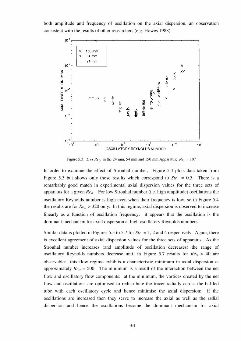
5:4
both amplitude and frequency of oscillation on the axial dispersion, an observation
consistent with the results of other researchers (e.g. Howes 1988).
Figure 5.3: E vs Reo in the 24 mm, 54 mm and 150 mm Apparatus; Ren = 107
In order to examine the effect of Strouhal number, Figure 5.4 plots data taken from
Figure 5.3 but shows only those results which correspond to Str = 0.5. There is a
remarkably good match in experimental axial dispersion values for the three sets of
apparatus for a given Reo . For low Strouhal number (i.e. high amplitude) oscillations the
oscillatory Reynolds number is high even when their frequency is low, so in Figure 5.4
the results are for Reo > 320 only. In this regime, axial dispersion is observed to increase
linearly as a function of oscillation frequency; it appears that the oscillation is the
dominant mechanism for axial dispersion at high oscillatory Reynolds numbers.
Similar data is plotted in Figures 5.5 to 5.7 for Str = 1, 2 and 4 respectively. Again, there
is excellent agreement of axial dispersion values for the three sets of apparatus. As the
Strouhal number increases (and amplitude of oscillation decreases) the range of
oscillatory Reynolds numbers decrease until in Figure 5.7 results for Reo > 40 are
observable: this flow regime exhibits a characteristic minimum in axial dispersion at
approximately Reo = 500. The minimum is a result of the interaction between the net
flow and oscillatory flow components: at the minimum, the vortices created by the net
flow and oscillations are optimised to redistribute the tracer radially across the baffled
tube with each oscillatory cycle and hence minimise the axial dispersion; if the
oscillations are increased then they serve to increase the axial as well as the radial
dispersion and hence the oscillations become the dominant mechanism for axial
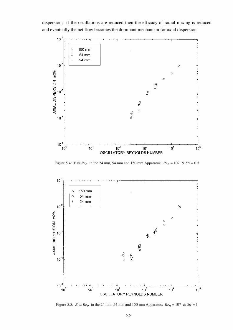
5:5
dispersion; if the oscillations are reduced then the efficacy of radial mixing is reduced
and eventually the net flow becomes the dominant mechanism for axial dispersion.
Figure 5.4: E vs Reo in the 24 mm, 54 mm and 150 mm Apparatus; Ren = 107 & Str = 0.5
Figure 5.5: E vs Reo in the 24 mm, 54 mm and 150 mm Apparatus; Ren = 107 & Str = 1
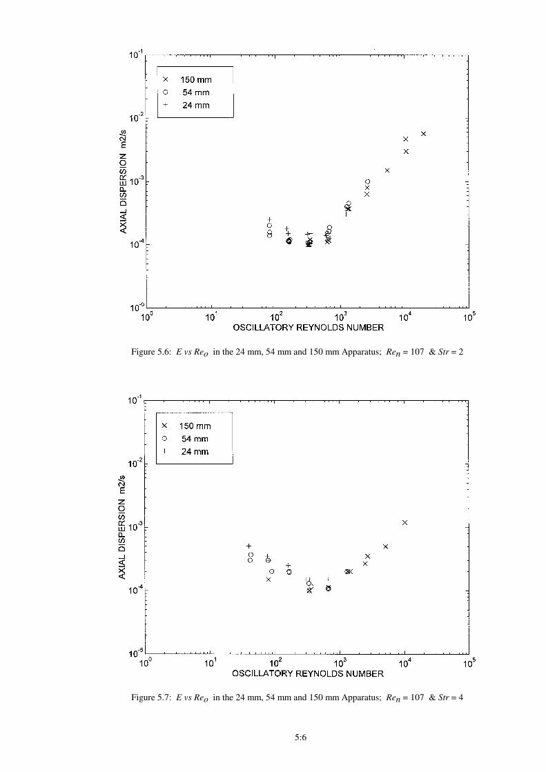
5:6
Figure 5.6: E vs Reo in the 24 mm, 54 mm and 150 mm Apparatus; Ren = 107 & Str = 2
Figure 5.7: E vs Reo in the 24 mm, 54 mm and 150 mm Apparatus; Ren = 107 & Str = 4
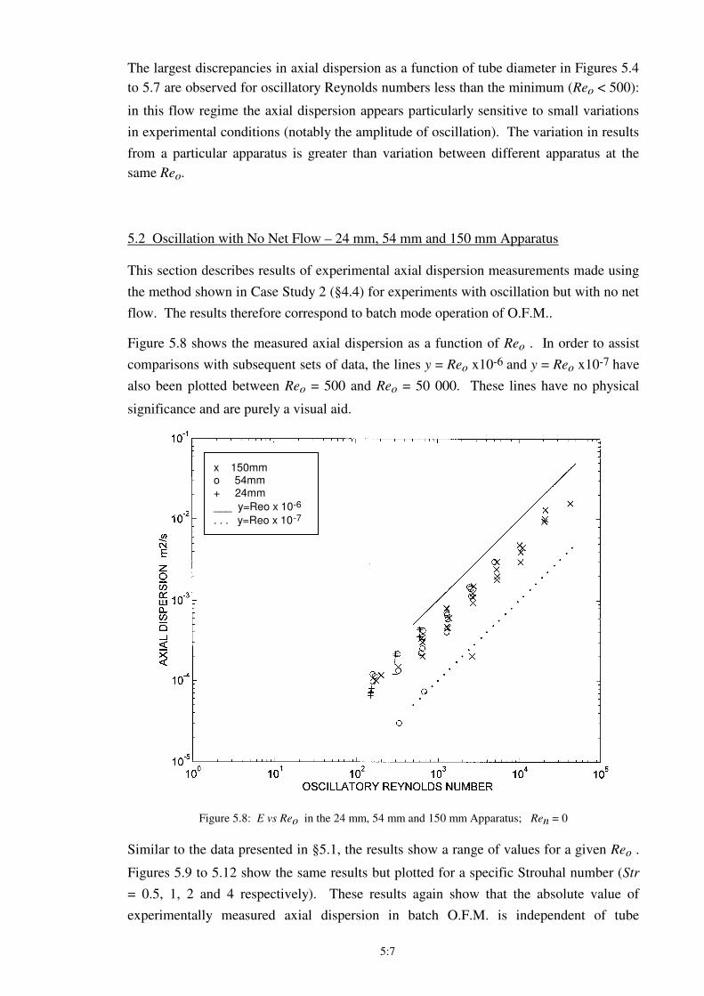
5:7
The largest discrepancies in axial dispersion as a function of tube diameter in Figures 5.4
to 5.7 are observed for oscillatory Reynolds numbers less than the minimum (Reo < 500):
in this flow regime the axial dispersion appears particularly sensitive to small variations
in experimental conditions (notably the amplitude of oscillation). The variation in results
from a particular apparatus is greater than variation between different apparatus at the
same Reo.
5.2 Oscillation with No Net Flow – 24 mm, 54 mm and 150 mm Apparatus
This section describes results of experimental axial dispersion measurements made using
the method shown in Case Study 2 (§4.4) for experiments with oscillation but with no net
flow. The results therefore correspond to batch mode operation of O.F.M..
Figure 5.8 shows the measured axial dispersion as a function of Reo . In order to assist
comparisons with subsequent sets of data, the lines y = Reo x10-6 and y = Reo x10-7 have
also been plotted between Reo = 500 and Reo = 50 000. These lines have no physical
significance and are purely a visual aid.
x 150mmo 54mm+ 24mm
___ y=Reo x 10-6
. . . y=Reo x 10-7
Figure 5.8: E vs Reo in the 24 mm, 54 mm and 150 mm Apparatus; Ren = 0
Similar to the data presented in §5.1, the results show a range of values for a given Reo .
Figures 5.9 to 5.12 show the same results but plotted for a specific Strouhal number (Str
= 0.5, 1, 2 and 4 respectively). These results again show that the absolute value of
experimentally measured axial dispersion in batch O.F.M. is independent of tube
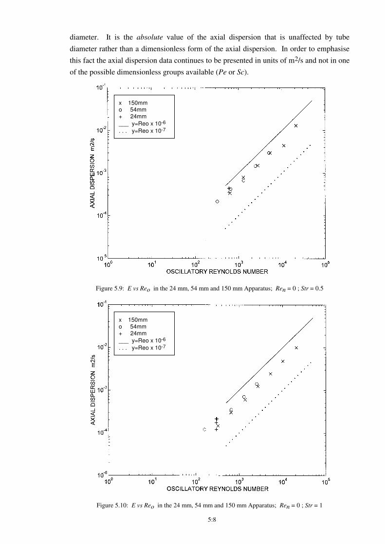
5:8
diameter. It is the absolute value of the axial dispersion that is unaffected by tube
diameter rather than a dimensionless form of the axial dispersion. In order to emphasise
this fact the axial dispersion data continues to be presented in units of m2/s and not in one
of the possible dimensionless groups available (Pe or Sc).
x 150mmo 54mm+ 24mm
___ y=Reo x 10-6
. . . y=Reo x 10-7
Figure 5.9: E vs Reo in the 24 mm, 54 mm and 150 mm Apparatus; Ren = 0 ; Str = 0.5
x 150mmo 54mm+ 24mm
___ y=Reo x 10-6
. . . y=Reo x 10-7
Figure 5.10: E vs Reo in the 24 mm, 54 mm and 150 mm Apparatus; Ren = 0 ; Str = 1
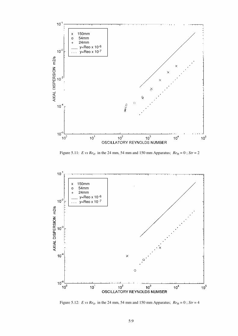
5:9
x 150mmo 54mm+ 24mm
___ y=Reo x 10-6
. . . y=Reo x 10-7
Figure 5.11: E vs Reo in the 24 mm, 54 mm and 150 mm Apparatus; Ren = 0 ; Str = 2
x 150mmo 54mm+ 24mm
___ y=Reo x 10 -6
. . . y=Reo x 10 -7
Figure 5.12: E vs Reo in the 24 mm, 54 mm and 150 mm Apparatus; Ren = 0 ; Str = 4
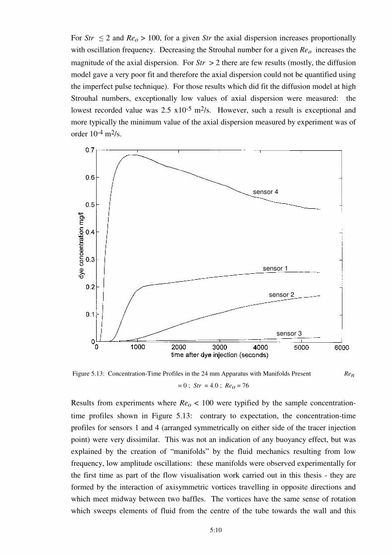
5:10
For Str ≤ 2 and Reo > 100, for a given Str the axial dispersion increases proportionally
with oscillation frequency. Decreasing the Strouhal number for a given Reo increases the
magnitude of the axial dispersion. For Str > 2 there are few results (mostly, the diffusion
model gave a very poor fit and therefore the axial dispersion could not be quantified using
the imperfect pulse technique). For those results which did fit the diffusion model at high
Strouhal numbers, exceptionally low values of axial dispersion were measured: the
lowest recorded value was 2.5 x10⁻⁵ m2/s. However, such a result is exceptional and
more typically the minimum value of the axial dispersion measured by experiment was of
order 10-4 m2/s.
sensor 4
sensor 3
sensor 2
sensor 1
Figure 5.13: Concentration-Time Profiles in the 24 mm Apparatus with Manifolds Present Ren
= 0 ; Str = 4.0 ; Reo = 76
Results from experiments where Reo < 100 were typified by the sample concentration-
time profiles shown in Figure 5.13: contrary to expectation, the concentration-time
profiles for sensors 1 and 4 (arranged symmetrically on either side of the tracer injection
point) were very dissimilar. This was not an indication of any buoyancy effect, but was
explained by the creation of “manifolds” by the fluid mechanics resulting from low
frequency, low amplitude oscillations: these manifolds were observed experimentally for
the first time as part of the flow visualisation work carried out in this thesis - they are
formed by the interaction of axisymmetric vortices travelling in opposite directions and
which meet midway between two baffles. The vortices have the same sense of rotation
which sweeps elements of fluid from the centre of the tube towards the wall and this
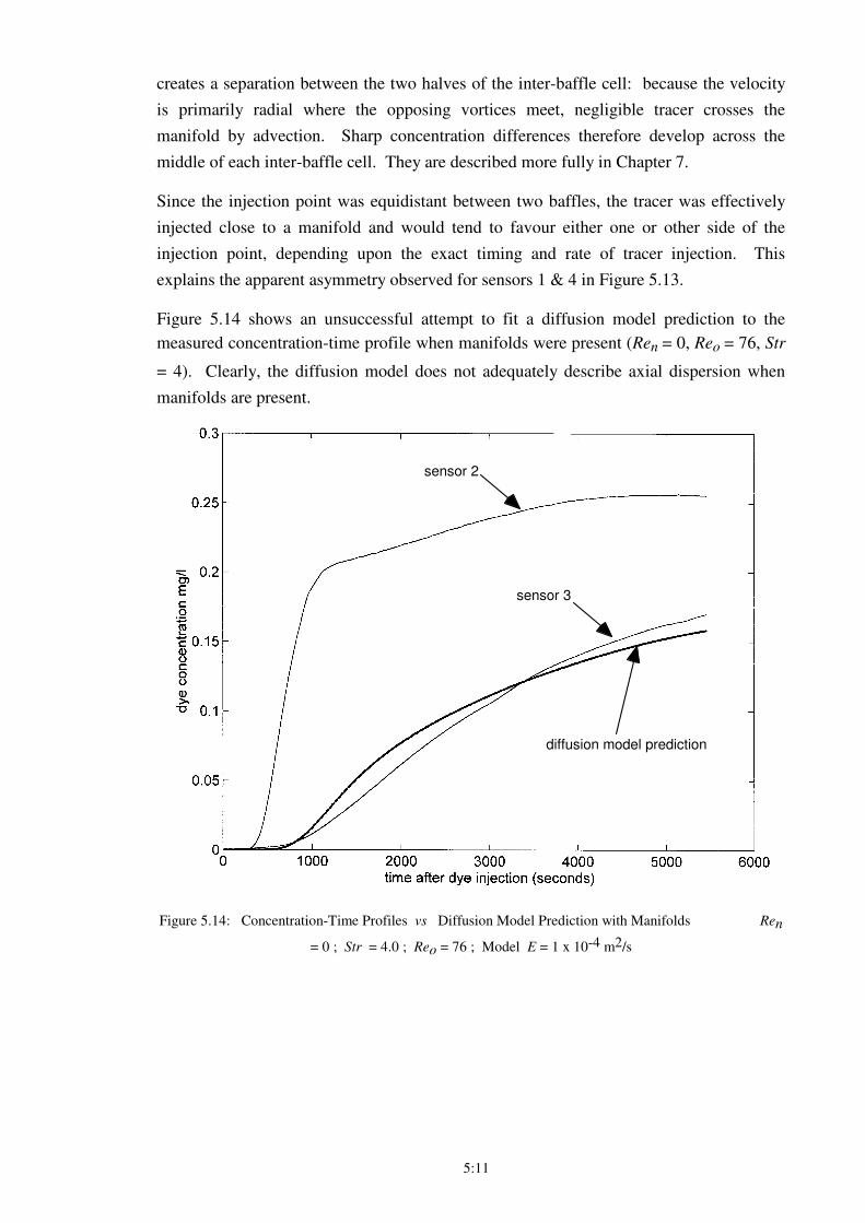
5:11
creates a separation between the two halves of the inter-baffle cell: because the velocity
is primarily radial where the opposing vortices meet, negligible tracer crosses the
manifold by advection. Sharp concentration differences therefore develop across the
middle of each inter-baffle cell. They are described more fully in Chapter 7.
Since the injection point was equidistant between two baffles, the tracer was effectively
injected close to a manifold and would tend to favour either one or other side of the
injection point, depending upon the exact timing and rate of tracer injection. This
explains the apparent asymmetry observed for sensors 1 & 4 in Figure 5.13.
Figure 5.14 shows an unsuccessful attempt to fit a diffusion model prediction to the
measured concentration-time profile when manifolds were present (Ren = 0, Reo = 76, Str
= 4). Clearly, the diffusion model does not adequately describe axial dispersion when
manifolds are present.
sensor 2
sensor 3
diffusion model prediction
Figure 5.14: Concentration-Time Profiles vs Diffusion Model Prediction with Manifolds Ren
= 0 ; Str = 4.0 ; Reo = 76 ; Model E = 1 x 10⁻⁴ m2/s
5:12
5.3 Net Flow with No Oscillation – 24 mm, 54 mm and 150 mm Apparatus
Figure 5.15 shows the results of experimental axial dispersion measurements made using
the method shown in Case Study 1 (§4.3) for experiments with net flow but no
oscillation. This corresponds to regular pipe flow with a series of flow restrictions (the
baffles).
x 150mmo 54mm+ 24mm
___ y=Reo x 10-6
. . . y=Reo x 10-7
Figure 5.15: E vs Ren in the 24 mm, 54 mm and 150 mm Apparatus; Reo = 0
For Ren ≥ 400 the measured axial dispersion increases proportionally with Ren . For Ren
< 400 there are large discrepancies in the results for the three sets of apparatus. This is
thought to be a reflection of the unreliability of vortex-formation at these low Reynolds
number flows for a non-reversing flow (without oscillation). Under these conditions,
non-oscillatory flow mixing appears to be susceptible to very small changes in net
flowrate, baffle orifice construction and possibly vibration from the lab surroundings all
of which can affect vortex formation at the baffle orifice.
For Ren < 100 there is little or no vortex formation and the diffusion equation does not
adequately model over short distances what is essentially a Poiseuille-type flow (see
Chapter 7). Under these conditions the axial dispersion cannot be quantified using the
imperfect pulse technique.
5:13
Interestingly, the measured axial dispersion for a particular Reynolds number (net flow or
oscillatory) is greater for a pure net flow than for a pure oscillation (comparing Figures
5.15 and 5.8). This illustrates the effectiveness of O.F.M. at minimising axial dispersion.
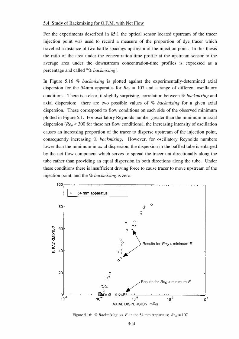
5:14
5.4 Study of Backmixing for O.F.M. with Net Flow
For the experiments described in §5.1 the optical sensor located upstream of the tracer
injection point was used to record a measure of the proportion of dye tracer which
travelled a distance of two baffle-spacings upstream of the injection point. In this thesis
the ratio of the area under the concentration-time profile at the upstream sensor to the
average area under the downstream concentration-time profiles is expressed as a
percentage and called "% backmixing".
In Figure 5.16 % backmixing is plotted against the experimentally-determined axial
dispersion for the 54mm apparatus for Ren = 107 and a range of different oscillatory
conditions. There is a clear, if slightly surprising, correlation between % backmixing and
axial dispersion: there are two possible values of % backmixing for a given axial
dispersion. These correspond to flow conditions on each side of the observed minimum
plotted in Figure 5.1. For oscillatory Reynolds number greater than the minimum in axial
dispersion (Reo ≥ 300 for these net flow conditions), the increasing intensity of oscillation
causes an increasing proportion of the tracer to disperse upstream of the injection point,
consequently increasing % backmixing. However, for oscillatory Reynolds numbers
lower than the minimum in axial dispersion, the dispersion in the baffled tube is enlarged
by the net flow component which serves to spread the tracer uni-directionally along the
tube rather than providing an equal dispersion in both directions along the tube. Under
these conditions there is insufficient driving force to cause tracer to move upstream of the
injection point, and the % backmixing is zero.
Results for Reo > minimum E
Results for Reo < minimum E
AXIAL DISPERSION m2/s
Figure 5.16: % Backmixing vs E in the 54 mm Apparatus; Ren = 107
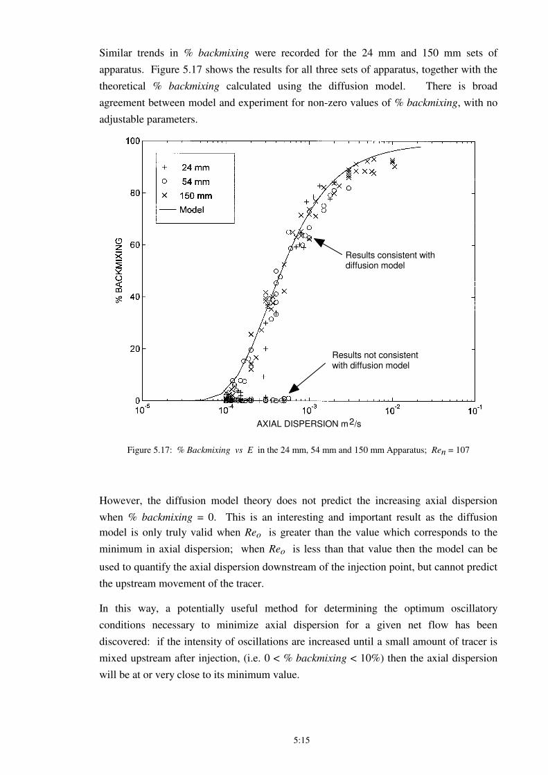
5:15
Similar trends in % backmixing were recorded for the 24 mm and 150 mm sets of
apparatus. Figure 5.17 shows the results for all three sets of apparatus, together with the
theoretical % backmixing calculated using the diffusion model. There is broad
agreement between model and experiment for non-zero values of % backmixing, with no
adjustable parameters.
Results consistent with diffusion model
Results not consistentwith diffusion model
AXIAL DISPERSION m2/s
Figure 5.17: % Backmixing vs E in the 24 mm, 54 mm and 150 mm Apparatus; Ren = 107
However, the diffusion model theory does not predict the increasing axial dispersion
when % backmixing = 0. This is an interesting and important result as the diffusion
model is only truly valid when Reo is greater than the value which corresponds to the
minimum in axial dispersion; when Reo is less than that value then the model can be
used to quantify the axial dispersion downstream of the injection point, but cannot predict
the upstream movement of the tracer.
In this way, a potentially useful method for determining the optimum oscillatory
conditions necessary to minimize axial dispersion for a given net flow has been
discovered: if the intensity of oscillations are increased until a small amount of tracer is
mixed upstream after injection, (i.e. 0 < % backmixing < 10%) then the axial dispersion
will be at or very close to its minimum value.
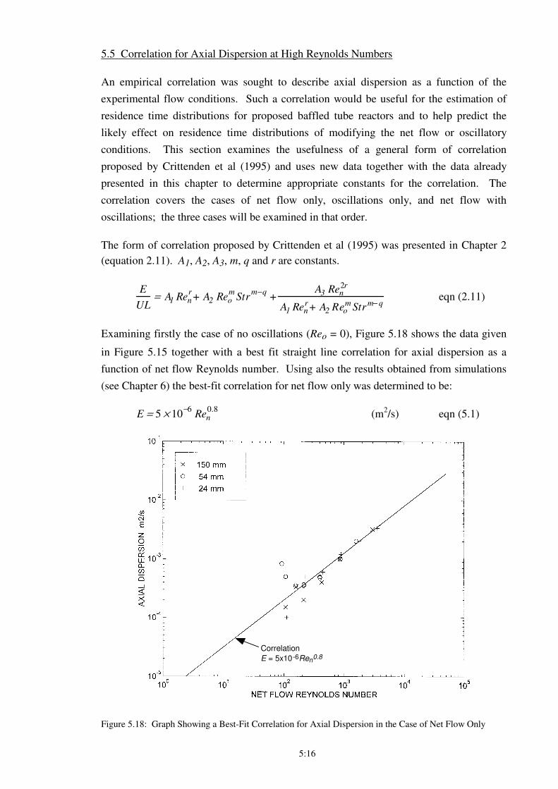
5:16
5.5 Correlation for Axial Dispersion at High Reynolds Numbers
An empirical correlation was sought to describe axial dispersion as a function of the
experimental flow conditions. Such a correlation would be useful for the estimation of
residence time distributions for proposed baffled tube reactors and to help predict the
likely effect on residence time distributions of modifying the net flow or oscillatory
conditions. This section examines the usefulness of a general form of correlation
proposed by Crittenden et al (1995) and uses new data together with the data already
presented in this chapter to determine appropriate constants for the correlation. The
correlation covers the cases of net flow only, oscillations only, and net flow with
oscillations; the three cases will be examined in that order.
The form of correlation proposed by Crittenden et al (1995) was presented in Chapter 2
(equation 2.11). A1, A2, A3, m, q and r are constants.
E
UL= A1 Ren
r+ A2 Reo
mStr
m−q+
A3 Ren2r
A1 Renr + A2 Reo
m Str m− q eqn (2.11)
Examining firstly the case of no oscillations (Reo = 0), Figure 5.18 shows the data given
in Figure 5.15 together with a best fit straight line correlation for axial dispersion as a
function of net flow Reynolds number. Using also the results obtained from simulations
(see Chapter 6) the best-fit correlation for net flow only was determined to be:
E = 5 × 10⁻⁶
Ren0.8
(m2/s) eqn (5.1)
Correlation
E = 5x10⁻⁶Ren0.8
Figure 5.18: Graph Showing a Best-Fit Correlation for Axial Dispersion in the Case of Net Flow Only
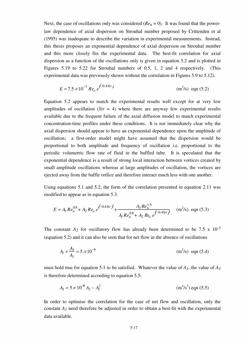
5:17
Next, the case of oscillations only was considered (Ren = 0). It was found that the power-
law dependence of axial dispersion on Strouhal number proposed by Crittenden et al
(1995) was inadequate to describe the variation in experimental measurements. Instead,
this thesis proposes an exponential dependence of axial dispersion on Strouhal number
and this more closely fits the experimental data. The best-fit correlation for axial
dispersion as a function of the oscillations only is given in equation 5.2 and is plotted in
Figures 5.19 to 5.22 for Strouhal numbers of 0.5, 1, 2 and 4 respectively. (This
experimental data was previously shown without the correlation in Figures 5.9 to 5.12).
E = 7.5 × 10⁻⁷
Reo e−0.4Str( )
(m2/s) eqn (5.2)
Equation 5.2 appears to match the experimental results well except for at very low
amplitudes of oscillation (Str = 4) where there are anyway few experimental results
available due to the frequent failure of the axial diffusion model to match experimental
concentration-time profiles under these conditions. It is not immediately clear why the
axial dispersion should appear to have an exponential dependence upon the amplitude of
oscillation; a first-order model might have assumed that the dispersion would be
proportional to both amplitude and frequency of oscillation i.e. proportional to the
periodic volumetric flow rate of fluid in the baffled tube. It is speculated that the
exponential dependence is a result of strong local interaction between vortices created by
small amplitude oscillations whereas at large amplitudes of oscillation, the vortices are
ejected away from the baffle orifice and therefore interact much less with one another.
Using equations 5.1 and 5.2, the form of the correlation presented in equation 2.11 was
modified to appear as in equation 5.3.
E = A1 Ren0.8
+ A2 Reo e−0.4Str( )
+A3 Ren
1.6
A1 Ren0.8
+ A2 Reo e−0.4Str( )
(m2/s) eqn (5.3)
The constant A2 for oscillatory flow has already been determined to be 7.5 x 10⁻⁷
(equation 5.2) and it can also be seen that for net flow in the absence of oscillations
A1 +A3
A1
= 5 × 10⁻⁶
(m2/s) eqn (5.4)
must hold true for equation 5.1 to be satisfied. Whatever the value of A1, the value of A3
is therefore determined according to equation 5.5:
A3 = 5× 10
−6A1 − A1
2 (m
4/s
2) eqn (5.5)
In order to optimise the correlation for the case of net flow and oscillation, only the
constant A1 need therefore be adjusted in order to obtain a best-fit with the experimental
data available.
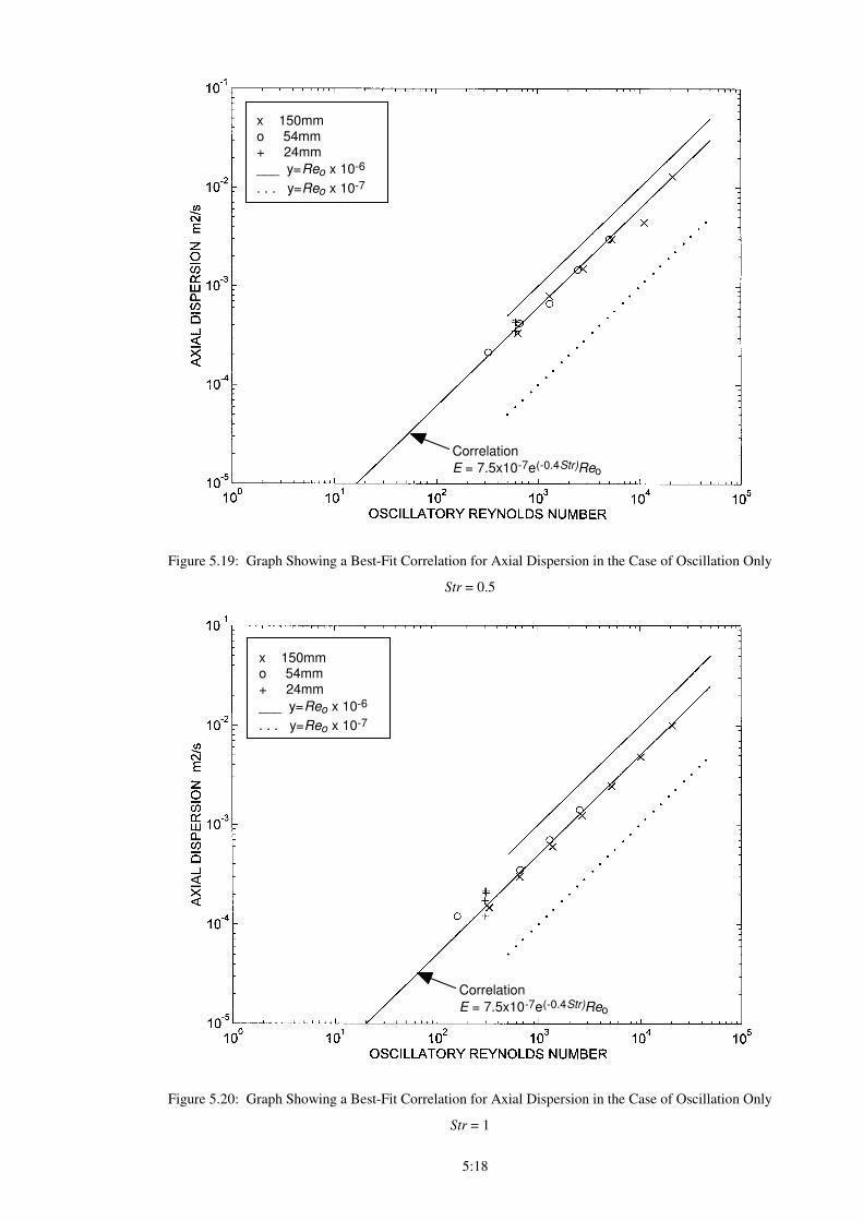
5:18
x 150mmo 54mm+ 24mm
___ y=Reo x 10-6
. . . y=Reo x 10-7
Correlation
E = 7.5x10⁻⁷e(-0.4Str)Reo
Figure 5.19: Graph Showing a Best-Fit Correlation for Axial Dispersion in the Case of Oscillation Only
Str = 0.5
Correlation
E = 7.5x10⁻⁷e(-0.4Str)Reo
x 150mmo 54mm+ 24mm
___ y=Reo x 10-6
. . . y=Reo x 10-7
Figure 5.20: Graph Showing a Best-Fit Correlation for Axial Dispersion in the Case of Oscillation Only
Str = 1
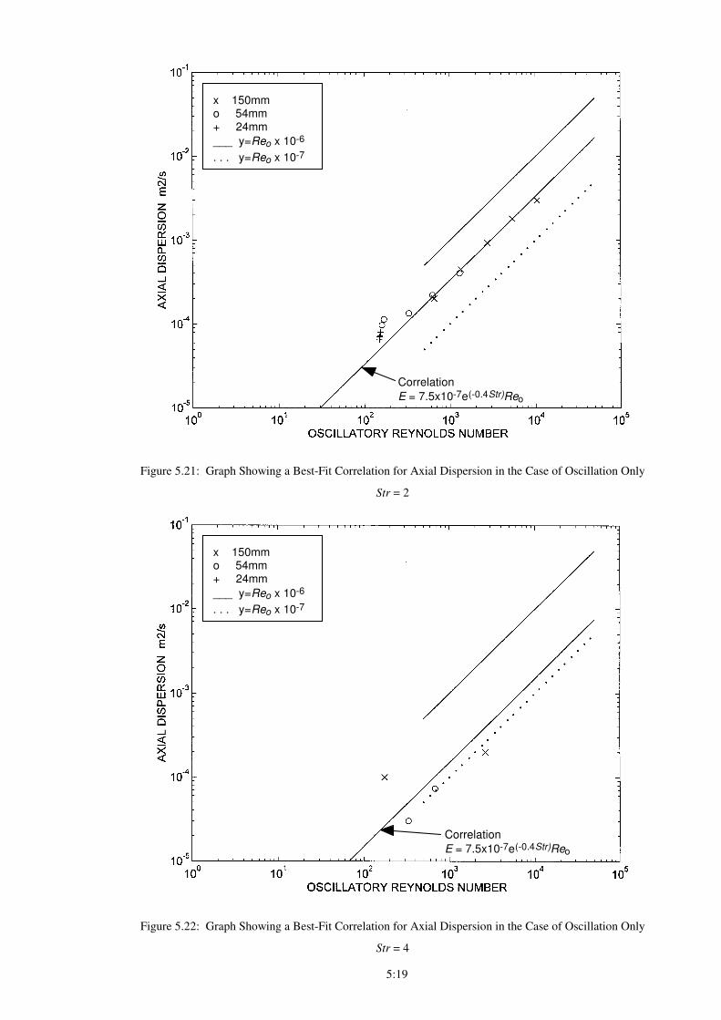
5:19
Correlation
E = 7.5x10⁻⁷e(-0.4Str)Reo
x 150mmo 54mm+ 24mm
___ y=Reo x 10-6
. . . y=Reo x 10-7
Figure 5.21: Graph Showing a Best-Fit Correlation for Axial Dispersion in the Case of Oscillation Only
Str = 2
Correlation
E = 7.5x10⁻⁷e(-0.4Str)Reo
x 150mmo 54mm+ 24mm
___ y=Reo x 10-6
. . . y=Reo x 10-7
Figure 5.22: Graph Showing a Best-Fit Correlation for Axial Dispersion in the Case of Oscillation Only
Str = 4
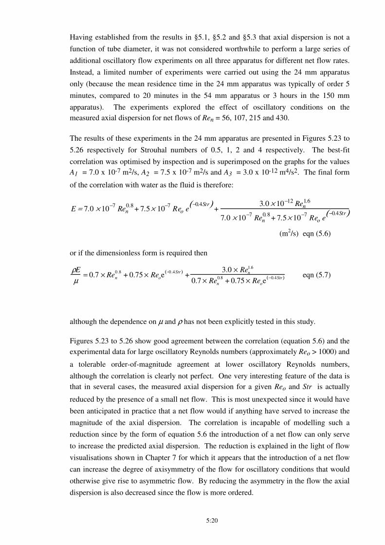
5:20
Having established from the results in §5.1, §5.2 and §5.3 that axial dispersion is not a
function of tube diameter, it was not considered worthwhile to perform a large series of
additional oscillatory flow experiments on all three apparatus for different net flow rates.
Instead, a limited number of experiments were carried out using the 24 mm apparatus
only (because the mean residence time in the 24 mm apparatus was typically of order 5
minutes, compared to 20 minutes in the 54 mm apparatus or 3 hours in the 150 mm
apparatus). The experiments explored the effect of oscillatory conditions on the
measured axial dispersion for net flows of Ren = 56, 107, 215 and 430.
The results of these experiments in the 24 mm apparatus are presented in Figures 5.23 to
5.26 respectively for Strouhal numbers of 0.5, 1, 2 and 4 respectively. The best-fit
correlation was optimised by inspection and is superimposed on the graphs for the values
A1 = 7.0 x 10⁻⁷ m2/s, A2 = 7.5 x 10⁻⁷ m2/s and A3 = 3.0 x 10⁻¹² m4/s2. The final form
of the correlation with water as the fluid is therefore:
E = 7.0 × 10⁻⁷
Ren0.8
+ 7.5× 10⁻⁷
Reo e−0.4Str( )
+3.0 × 10⁻¹² Ren
1.6
7.0 × 10⁻⁷
Ren0.8
+ 7.5× 10⁻⁷
Reo e−0.4Str( )
(m2/s) eqn (5.6)
or if the dimensionless form is required then
ρE
µ= 0.7 × Ren
0.8+ 0.75 × Reoe
−0.4Str( )+
3.0 × Ren
1.6
0.7 × Ren
0.8+ 0.75 × Reoe
−0.4Str( ) eqn (5.7)
although the dependence on µ and ρ has not been explicitly tested in this study.
Figures 5.23 to 5.26 show good agreement between the correlation (equation 5.6) and the
experimental data for large oscillatory Reynolds numbers (approximately Reo > 1000) and
a tolerable order-of-magnitude agreement at lower oscillatory Reynolds numbers,
although the correlation is clearly not perfect. One very interesting feature of the data is
that in several cases, the measured axial dispersion for a given Reo and Str is actually
reduced by the presence of a small net flow. This is most unexpected since it would have
been anticipated in practice that a net flow would if anything have served to increase the
magnitude of the axial dispersion. The correlation is incapable of modelling such a
reduction since by the form of equation 5.6 the introduction of a net flow can only serve
to increase the predicted axial dispersion. The reduction is explained in the light of flow
visualisations shown in Chapter 7 for which it appears that the introduction of a net flow
can increase the degree of axisymmetry of the flow for oscillatory conditions that would
otherwise give rise to asymmetric flow. By reducing the asymmetry in the flow the axial
dispersion is also decreased since the flow is more ordered.
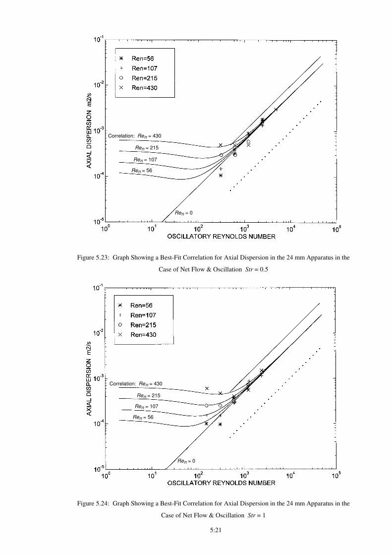
5:21
Correlation: Ren = 430
Ren = 215
Ren = 107
Ren = 56
Ren = 0
Figure 5.23: Graph Showing a Best-Fit Correlation for Axial Dispersion in the 24 mm Apparatus in the
Case of Net Flow & Oscillation Str = 0.5
Correlation: Ren = 430
Ren = 215
Ren = 107
Ren = 56
Ren = 0
Figure 5.24: Graph Showing a Best-Fit Correlation for Axial Dispersion in the 24 mm Apparatus in the
Case of Net Flow & Oscillation Str = 1
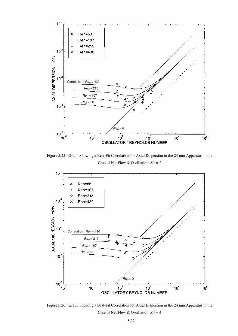
5:22
Correlation: Ren = 430
Ren = 215
Ren = 107
Ren = 56
Ren = 0
Figure 5.25: Graph Showing a Best-Fit Correlation for Axial Dispersion in the 24 mm Apparatus in the
Case of Net Flow & Oscillation Str = 2
Correlation: Ren = 430
Ren = 215
Ren = 107
Ren = 56
Ren = 0
Figure 5.26: Graph Showing a Best-Fit Correlation for Axial Dispersion in the 24 mm Apparatus in the
Case of Net Flow & Oscillation Str = 4
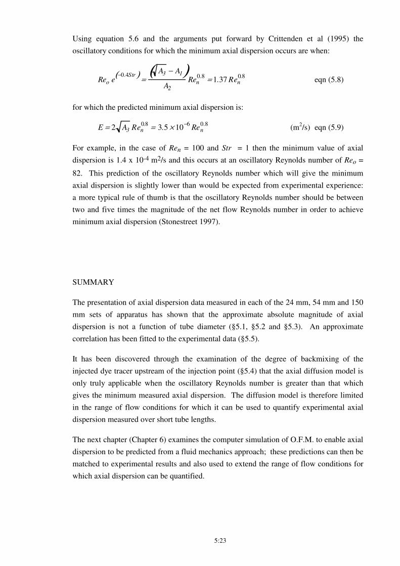
5:23
Using equation 5.6 and the arguments put forward by Crittenden et al (1995) the
oscillatory conditions for which the minimum axial dispersion occurs are when:
Reo e−0.4Str( )
=A3 − A1( )
A2
Ren0.8
= 1.37 Ren0.8
eqn (5.8)
for which the predicted minimum axial dispersion is:
E = 2 A3 Ren0.8
= 3.5 × 10⁻⁶
Ren0.8
(m2/s) eqn (5.9)
For example, in the case of Ren = 100 and Str = 1 then the minimum value of axial
dispersion is 1.4 x 10⁻⁴ m2/s and this occurs at an oscillatory Reynolds number of Reo =
82. This prediction of the oscillatory Reynolds number which will give the minimum
axial dispersion is slightly lower than would be expected from experimental experience:
a more typical rule of thumb is that the oscillatory Reynolds number should be between
two and five times the magnitude of the net flow Reynolds number in order to achieve
minimum axial dispersion (Stonestreet 1997).
SUMMARY
The presentation of axial dispersion data measured in each of the 24 mm, 54 mm and 150
mm sets of apparatus has shown that the approximate absolute magnitude of axial
dispersion is not a function of tube diameter (§5.1, §5.2 and §5.3). An approximate
correlation has been fitted to the experimental data (§5.5).
It has been discovered through the examination of the degree of backmixing of the
injected dye tracer upstream of the injection point (§5.4) that the axial diffusion model is
only truly applicable when the oscillatory Reynolds number is greater than that which
gives the minimum measured axial dispersion. The diffusion model is therefore limited
in the range of flow conditions for which it can be used to quantify experimental axial
dispersion measured over short tube lengths.
The next chapter (Chapter 6) examines the computer simulation of O.F.M. to enable axial
dispersion to be predicted from a fluid mechanics approach; these predictions can then be
matched to experimental results and also used to extend the range of flow conditions for
which axial dispersion can be quantified.

6:1
6. Axial Dispersion Measurements from Fluid Mechanical Simulation
The chapters so far in this thesis have dealt with the experimental measurement and
quantification of axial dispersion in O.F.M.. The range of experimental conditions
studied was restricted for low Reynolds number flows by the limits of the diffusion
model which could not always successfully model experimental concentration profiles. It
would therefore be advantageous to be able to predict the axial dispersion of tracer in
O.F.M. at low Reynolds numbers (< 300) from fundamental principles: this chapter
investigates the prediction of axial dispersion in single-phase O.F.M. using a numerical
fluid mechanical simulation. Values of axial dispersion predicted by the fluid mechanical
simulation are compared with those measured experimentally and the simulation is used
to extend the range of results for flow conditions where the diffusion model did not match
the experimental results. The range of overlap between experiment and simulation also
improves confidence in both the experimental and simulated results.
The chapter is divided into two sections: §6.1 presents the method by which axial
dispersion was modelled using the injection of fluid marker particles into the numerically
simulated flow field. Two different approaches were used to try to quantify axial
dispersion using the results of the simulation:
i) the imperfect pulse technique, and
ii) the rate of change of particle variance.
Results obtained using the second (preferred) method are presented in §6.2 and are
compared with experimental results.
6.1 Simulation of Axial Dispersion in OFM Using Fluid Marker Particles
The finite difference fluid mechanical simulation developed by Dr R. Saraiva (1997) was
generously made available for use in this thesis. The simulation is written in Fortran
code and was run on an Ultra 170MHz Sun workstation; details of the programme are
given in Appendix VI. The simulation is based entirely upon the dimensionless groups
Reo, Ren and Str in order to define the fluid dynamic conditions and it therefore pre-
supposes that there is no dependence upon tube diameter as has been experimentally
confirmed in the previous chapter. Experimental results in the previous chapter covered a
large range of dynamic conditions, with 10 < Reo < 30 000. In comparison, the
simulation is restricted to axisymmetric flow and is therefore thought to be limited to Reo
≤ 300.
Numerical simulations were carried out for the cases of net flow only, oscillations only
and net flow with oscillations. In order to model experimental axial dispersion, a cloud
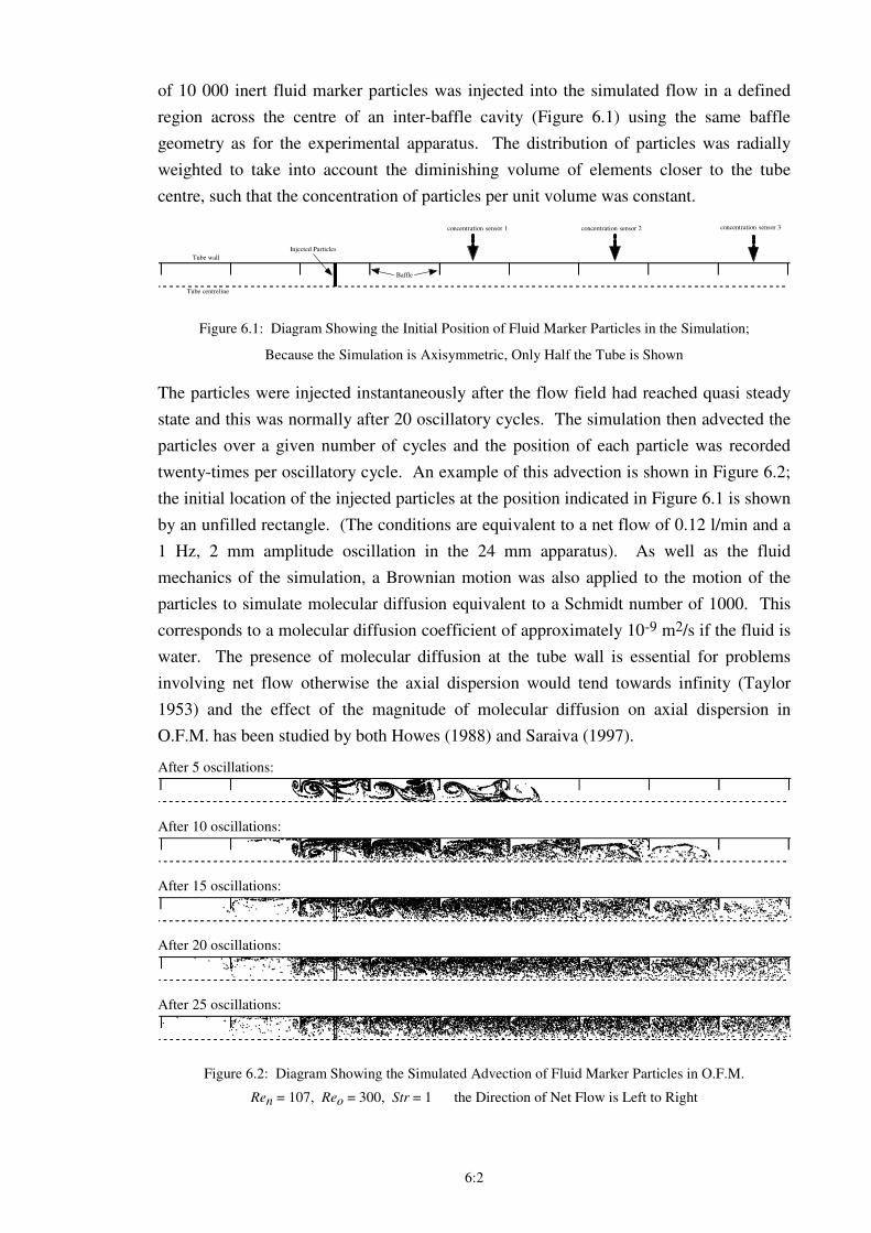
6:2
of 10 000 inert fluid marker particles was injected into the simulated flow in a defined
region across the centre of an inter-baffle cavity (Figure 6.1) using the same baffle
geometry as for the experimental apparatus. The distribution of particles was radially
weighted to take into account the diminishing volume of elements closer to the tube
centre, such that the concentration of particles per unit volume was constant.
Injected Particles
Tube wall
Baffle
Tube centreline
concentration sensor 1 concentration sensor 2 concentration sensor 3
Figure 6.1: Diagram Showing the Initial Position of Fluid Marker Particles in the Simulation;
Because the Simulation is Axisymmetric, Only Half the Tube is Shown
The particles were injected instantaneously after the flow field had reached quasi steady
state and this was normally after 20 oscillatory cycles. The simulation then advected the
particles over a given number of cycles and the position of each particle was recorded
twenty-times per oscillatory cycle. An example of this advection is shown in Figure 6.2;
the initial location of the injected particles at the position indicated in Figure 6.1 is shown
by an unfilled rectangle. (The conditions are equivalent to a net flow of 0.12 l/min and a
1 Hz, 2 mm amplitude oscillation in the 24 mm apparatus). As well as the fluid
mechanics of the simulation, a Brownian motion was also applied to the motion of the
particles to simulate molecular diffusion equivalent to a Schmidt number of 1000. This
corresponds to a molecular diffusion coefficient of approximately 10-9 m2/s if the fluid is
water. The presence of molecular diffusion at the tube wall is essential for problems
involving net flow otherwise the axial dispersion would tend towards infinity (Taylor
1953) and the effect of the magnitude of molecular diffusion on axial dispersion in
O.F.M. has been studied by both Howes (1988) and Saraiva (1997).
After 5 oscillations:
After 10 oscillations:
After 15 oscillations:
After 20 oscillations:
After 25 oscillations:
Figure 6.2: Diagram Showing the Simulated Advection of Fluid Marker Particles in O.F.M.
Ren = 107, Reo = 300, Str = 1 the Direction of Net Flow is Left to Right
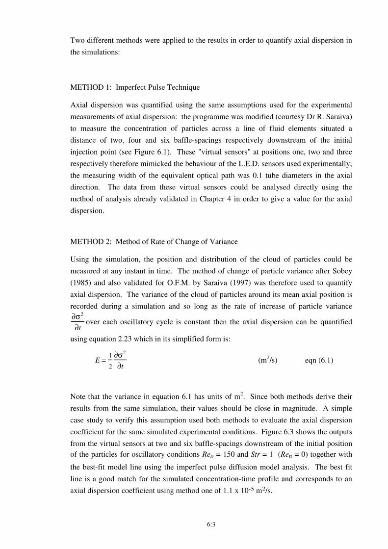
6:3
Two different methods were applied to the results in order to quantify axial dispersion in
the simulations:
METHOD 1: Imperfect Pulse Technique
Axial dispersion was quantified using the same assumptions used for the experimental
measurements of axial dispersion: the programme was modified (courtesy Dr R. Saraiva)
to measure the concentration of particles across a line of fluid elements situated a
distance of two, four and six baffle-spacings respectively downstream of the initial
injection point (see Figure 6.1). These "virtual sensors" at positions one, two and three
respectively therefore mimicked the behaviour of the L.E.D. sensors used experimentally;
the measuring width of the equivalent optical path was 0.1 tube diameters in the axial
direction. The data from these virtual sensors could be analysed directly using the
method of analysis already validated in Chapter 4 in order to give a value for the axial
dispersion.
METHOD 2: Method of Rate of Change of Variance
Using the simulation, the position and distribution of the cloud of particles could be
measured at any instant in time. The method of change of particle variance after Sobey
(1985) and also validated for O.F.M. by Saraiva (1997) was therefore used to quantify
axial dispersion. The variance of the cloud of particles around its mean axial position is
recorded during a simulation and so long as the rate of increase of particle variance
∂σ2
∂tover each oscillatory cycle is constant then the axial dispersion can be quantified
using equation 2.23 which in its simplified form is:
E =1
2
∂σ2
∂t (m
2/s) eqn (6.1)
Note that the variance in equation 6.1 has units of m2. Since both methods derive their
results from the same simulation, their values should be close in magnitude. A simple
case study to verify this assumption used both methods to evaluate the axial dispersion
coefficient for the same simulated experimental conditions. Figure 6.3 shows the outputs
from the virtual sensors at two and six baffle-spacings downstream of the initial position
of the particles for oscillatory conditions Reo = 150 and Str = 1 (Ren = 0) together with
the best-fit model line using the imperfect pulse diffusion model analysis. The best fit
line is a good match for the simulated concentration-time profile and corresponds to an
axial dispersion coefficient using method one of 1.1 x 10⁻⁵ m2/s.
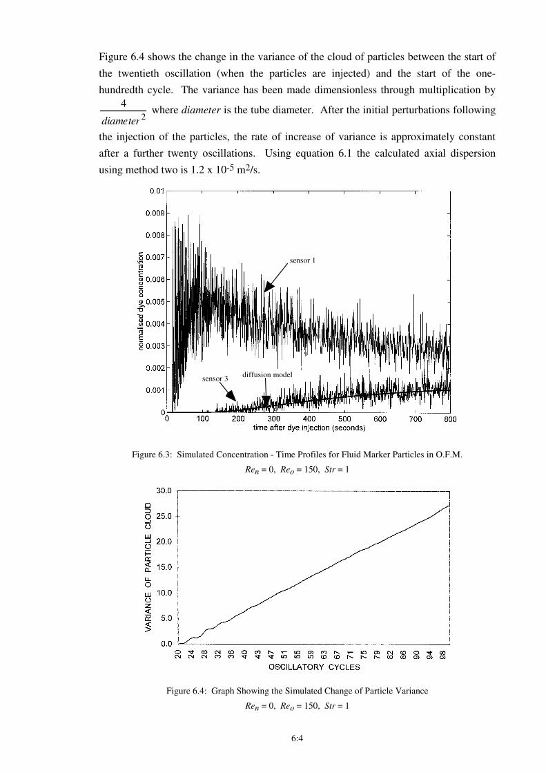
6:4
Figure 6.4 shows the change in the variance of the cloud of particles between the start of
the twentieth oscillation (when the particles are injected) and the start of the one-
hundredth cycle. The variance has been made dimensionless through multiplication by
4
diameter2
where diameter is the tube diameter. After the initial perturbations following
the injection of the particles, the rate of increase of variance is approximately constant
after a further twenty oscillations. Using equation 6.1 the calculated axial dispersion
using method two is 1.2 x 10⁻⁵ m2/s.
sensor 1
sensor 3diffusion model
Figure 6.3: Simulated Concentration - Time Profiles for Fluid Marker Particles in O.F.M.
Ren = 0, Reo = 150, Str = 1
Figure 6.4: Graph Showing the Simulated Change of Particle Variance
Ren = 0, Reo = 150, Str = 1
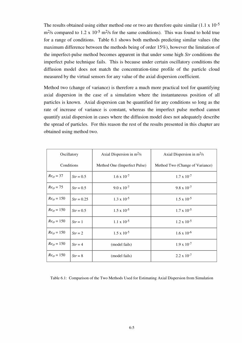
6:5
The results obtained using either method one or two are therefore quite similar (1.1 x 10⁻⁵
m2/s compared to 1.2 x 10⁻⁵ m2/s for the same conditions). This was found to hold true
for a range of conditions. Table 6.1 shows both methods predicting similar values (the
maximum difference between the methods being of order 15%), however the limitation of
the imperfect-pulse method becomes apparent in that under some high Str conditions the
imperfect pulse technique fails. This is because under certain oscillatory conditions the
diffusion model does not match the concentration-time profile of the particle cloud
measured by the virtual sensors for any value of the axial dispersion coefficient.
Method two (change of variance) is therefore a much more practical tool for quantifying
axial dispersion in the case of a simulation where the instantaneous position of all
particles is known. Axial dispersion can be quantified for any conditions so long as the
rate of increase of variance is constant, whereas the imperfect pulse method cannot
quantify axial dispersion in cases where the diffusion model does not adequately describe
the spread of particles. For this reason the rest of the results presented in this chapter are
obtained using method two.
Oscillatory
Conditions
Axial Dispersion in m2/s
Method One (Imperfect Pulse)
Axial Dispersion in m2/s
Method Two (Change of Variance)
Reo = 37 Str = 0.5 1.6 x 10⁻⁷ 1.7 x 10⁻⁷
Reo = 75 Str = 0.5 9.0 x 10⁻⁷ 9.8 x 10⁻⁷
Reo = 150 Str = 0.25 1.3 x 10⁻⁵ 1.5 x 10⁻⁵
Reo = 150 Str = 0.5 1.5 x 10⁻⁵ 1.7 x 10⁻⁵
Reo = 150 Str = 1 1.1 x 10⁻⁵ 1.2 x 10⁻⁵
Reo = 150 Str = 2 1.5 x 10⁻⁵ 1.6 x 10⁻⁶
Reo = 150 Str = 4 (model fails) 1.9 x 10⁻⁷
Reo = 150 Str = 8 (model fails) 2.2 x 10⁻⁷
Table 6.1: Comparison of the Two Methods Used for Estimating Axial Dispersion from Simulation
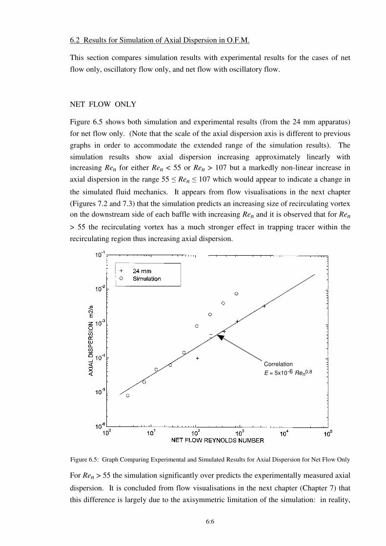
6:6
6.2 Results for Simulation of Axial Dispersion in O.F.M.
This section compares simulation results with experimental results for the cases of net
flow only, oscillatory flow only, and net flow with oscillatory flow.
NET FLOW ONLY
Figure 6.5 shows both simulation and experimental results (from the 24 mm apparatus)
for net flow only. (Note that the scale of the axial dispersion axis is different to previous
graphs in order to accommodate the extended range of the simulation results). The
simulation results show axial dispersion increasing approximately linearly with
increasing Ren for either Ren < 55 or Ren > 107 but a markedly non-linear increase in
axial dispersion in the range 55 ≤ Ren ≤ 107 which would appear to indicate a change in
the simulated fluid mechanics. It appears from flow visualisations in the next chapter
(Figures 7.2 and 7.3) that the simulation predicts an increasing size of recirculating vortex
on the downstream side of each baffle with increasing Ren and it is observed that for Ren
> 55 the recirculating vortex has a much stronger effect in trapping tracer within the
recirculating region thus increasing axial dispersion.
Correlation
E = 5x10⁻⁶ Ren0.8
Figure 6.5: Graph Comparing Experimental and Simulated Results for Axial Dispersion for Net Flow Only
For Ren > 55 the simulation significantly over predicts the experimentally measured axial
dispersion. It is concluded from flow visualisations in the next chapter (Chapter 7) that
this difference is largely due to the axisymmetric limitation of the simulation: in reality,
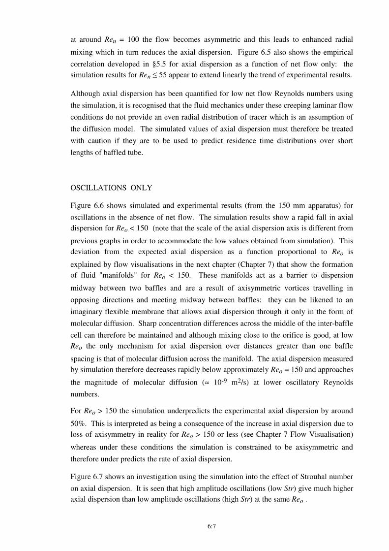
6:7
at around Ren = 100 the flow becomes asymmetric and this leads to enhanced radial
mixing which in turn reduces the axial dispersion. Figure 6.5 also shows the empirical
correlation developed in §5.5 for axial dispersion as a function of net flow only: the
simulation results for Ren ≤ 55 appear to extend linearly the trend of experimental results.
Although axial dispersion has been quantified for low net flow Reynolds numbers using
the simulation, it is recognised that the fluid mechanics under these creeping laminar flow
conditions do not provide an even radial distribution of tracer which is an assumption of
the diffusion model. The simulated values of axial dispersion must therefore be treated
with caution if they are to be used to predict residence time distributions over short
lengths of baffled tube.
OSCILLATIONS ONLY
Figure 6.6 shows simulated and experimental results (from the 150 mm apparatus) for
oscillations in the absence of net flow. The simulation results show a rapid fall in axial
dispersion for Reo < 150 (note that the scale of the axial dispersion axis is different from
previous graphs in order to accommodate the low values obtained from simulation). This
deviation from the expected axial dispersion as a function proportional to Reo is
explained by flow visualisations in the next chapter (Chapter 7) that show the formation
of fluid "manifolds" for Reo < 150. These manifolds act as a barrier to dispersion
midway between two baffles and are a result of axisymmetric vortices travelling in
opposing directions and meeting midway between baffles: they can be likened to an
imaginary flexible membrane that allows axial dispersion through it only in the form of
molecular diffusion. Sharp concentration differences across the middle of the inter-baffle
cell can therefore be maintained and although mixing close to the orifice is good, at low
Reo the only mechanism for axial dispersion over distances greater than one baffle
spacing is that of molecular diffusion across the manifold. The axial dispersion measured
by simulation therefore decreases rapidly below approximately Reo = 150 and approaches
the magnitude of molecular diffusion (≈ 10-9 m2/s) at lower oscillatory Reynolds
numbers.
For Reo > 150 the simulation underpredicts the experimental axial dispersion by around
50%. This is interpreted as being a consequence of the increase in axial dispersion due to
loss of axisymmetry in reality for Reo > 150 or less (see Chapter 7 Flow Visualisation)
whereas under these conditions the simulation is constrained to be axisymmetric and
therefore under predicts the rate of axial dispersion.
Figure 6.7 shows an investigation using the simulation into the effect of Strouhal number
on axial dispersion. It is seen that high amplitude oscillations (low Str) give much higher
axial dispersion than low amplitude oscillations (high Str) at the same Reo .
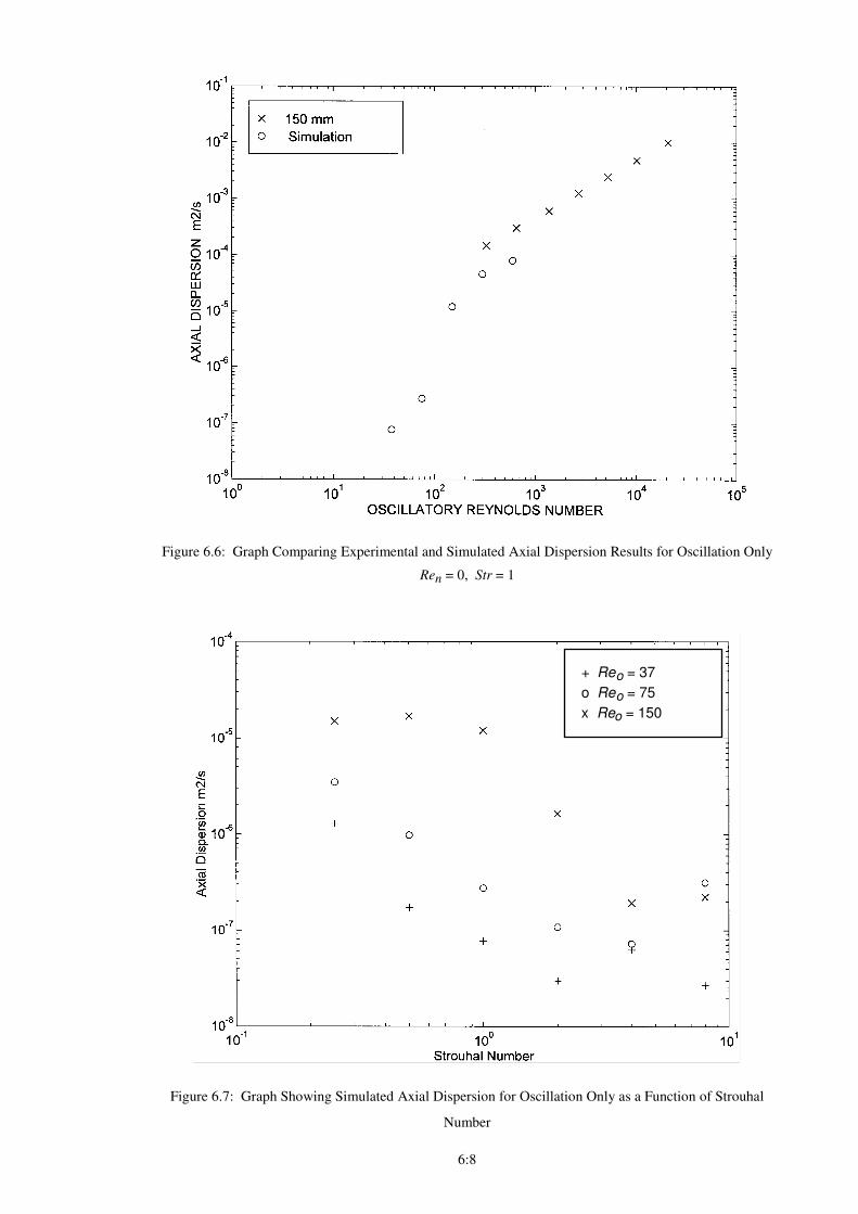
6:8
Figure 6.6: Graph Comparing Experimental and Simulated Axial Dispersion Results for Oscillation Only
Ren = 0, Str = 1
+ Reo = 37
o Reo = 75
x Reo = 150
Figure 6.7: Graph Showing Simulated Axial Dispersion for Oscillation Only as a Function of Strouhal
Number
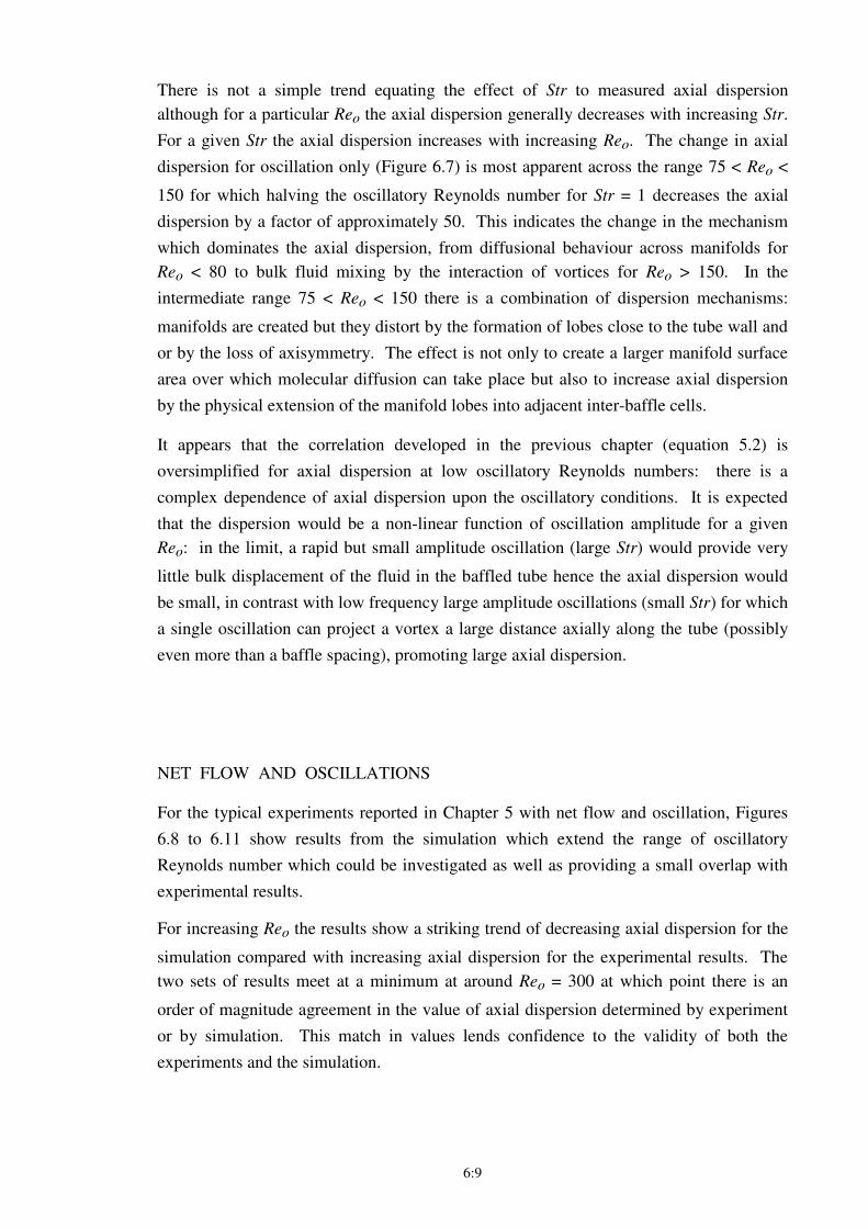
6:9
There is not a simple trend equating the effect of Str to measured axial dispersion
although for a particular Reo the axial dispersion generally decreases with increasing Str.
For a given Str the axial dispersion increases with increasing Reo. The change in axial
dispersion for oscillation only (Figure 6.7) is most apparent across the range 75 < Reo <
150 for which halving the oscillatory Reynolds number for Str = 1 decreases the axial
dispersion by a factor of approximately 50. This indicates the change in the mechanism
which dominates the axial dispersion, from diffusional behaviour across manifolds for
Reo < 80 to bulk fluid mixing by the interaction of vortices for Reo > 150. In the
intermediate range 75 < Reo < 150 there is a combination of dispersion mechanisms:
manifolds are created but they distort by the formation of lobes close to the tube wall and
or by the loss of axisymmetry. The effect is not only to create a larger manifold surface
area over which molecular diffusion can take place but also to increase axial dispersion
by the physical extension of the manifold lobes into adjacent inter-baffle cells.
It appears that the correlation developed in the previous chapter (equation 5.2) is
oversimplified for axial dispersion at low oscillatory Reynolds numbers: there is a
complex dependence of axial dispersion upon the oscillatory conditions. It is expected
that the dispersion would be a non-linear function of oscillation amplitude for a given
Reo: in the limit, a rapid but small amplitude oscillation (large Str) would provide very
little bulk displacement of the fluid in the baffled tube hence the axial dispersion would
be small, in contrast with low frequency large amplitude oscillations (small Str) for which
a single oscillation can project a vortex a large distance axially along the tube (possibly
even more than a baffle spacing), promoting large axial dispersion.
NET FLOW AND OSCILLATIONS
For the typical experiments reported in Chapter 5 with net flow and oscillation, Figures
6.8 to 6.11 show results from the simulation which extend the range of oscillatory
Reynolds number which could be investigated as well as providing a small overlap with
experimental results.
For increasing Reo the results show a striking trend of decreasing axial dispersion for the
simulation compared with increasing axial dispersion for the experimental results. The
two sets of results meet at a minimum at around Reo = 300 at which point there is an
order of magnitude agreement in the value of axial dispersion determined by experiment
or by simulation. This match in values lends confidence to the validity of both the
experiments and the simulation.
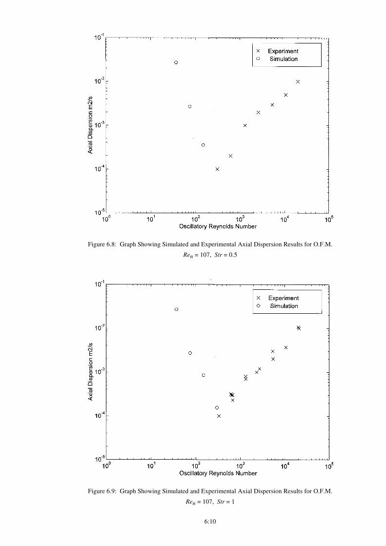
6:10
Figure 6.8: Graph Showing Simulated and Experimental Axial Dispersion Results for O.F.M.
Ren = 107, Str = 0.5
Figure 6.9: Graph Showing Simulated and Experimental Axial Dispersion Results for O.F.M.
Ren = 107, Str = 1
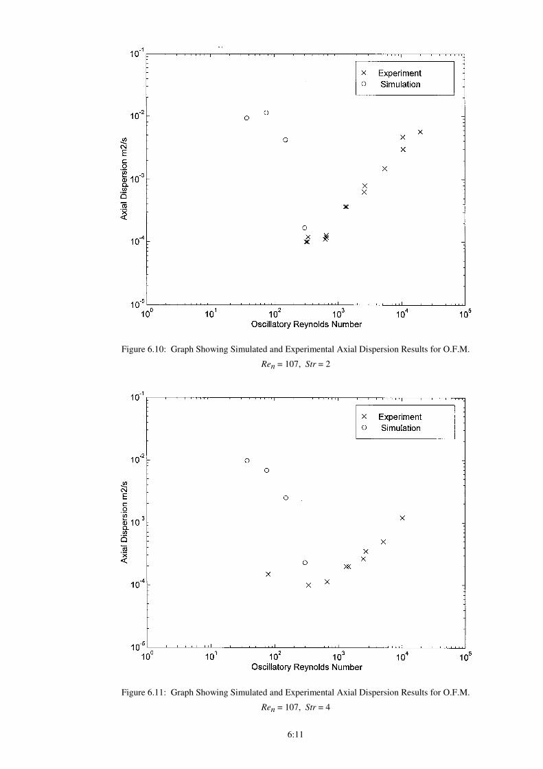
6:11
Figure 6.10: Graph Showing Simulated and Experimental Axial Dispersion Results for O.F.M.
Ren = 107, Str = 2
Figure 6.11: Graph Showing Simulated and Experimental Axial Dispersion Results for O.F.M.
Ren = 107, Str = 4
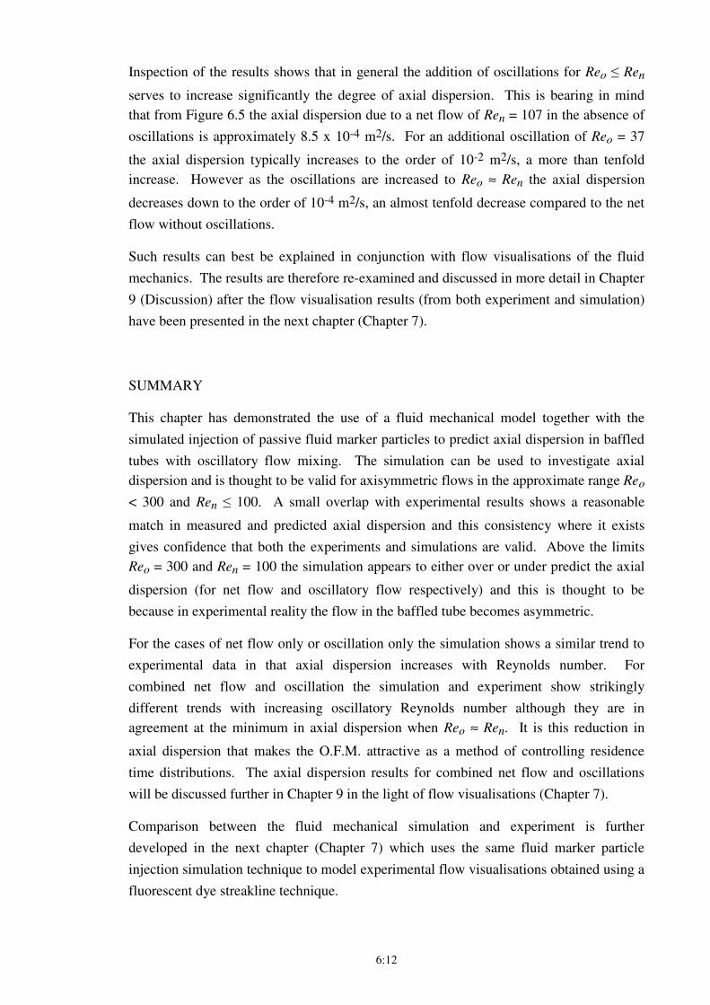
6:12
Inspection of the results shows that in general the addition of oscillations for Reo ≤ Ren
serves to increase significantly the degree of axial dispersion. This is bearing in mind
that from Figure 6.5 the axial dispersion due to a net flow of Ren = 107 in the absence of
oscillations is approximately 8.5 x 10⁻⁴ m2/s. For an additional oscillation of Reo = 37
the axial dispersion typically increases to the order of 10-2 m2/s, a more than tenfold
increase. However as the oscillations are increased to Reo ≈ Ren the axial dispersion
decreases down to the order of 10-4 m2/s, an almost tenfold decrease compared to the net
flow without oscillations.
Such results can best be explained in conjunction with flow visualisations of the fluid
mechanics. The results are therefore re-examined and discussed in more detail in Chapter
9 (Discussion) after the flow visualisation results (from both experiment and simulation)
have been presented in the next chapter (Chapter 7).
SUMMARY
This chapter has demonstrated the use of a fluid mechanical model together with the
simulated injection of passive fluid marker particles to predict axial dispersion in baffled
tubes with oscillatory flow mixing. The simulation can be used to investigate axial
dispersion and is thought to be valid for axisymmetric flows in the approximate range Reo
< 300 and Ren ≤ 100. A small overlap with experimental results shows a reasonable
match in measured and predicted axial dispersion and this consistency where it exists
gives confidence that both the experiments and simulations are valid. Above the limits
Reo = 300 and Ren = 100 the simulation appears to either over or under predict the axial
dispersion (for net flow and oscillatory flow respectively) and this is thought to be
because in experimental reality the flow in the baffled tube becomes asymmetric.
For the cases of net flow only or oscillation only the simulation shows a similar trend to
experimental data in that axial dispersion increases with Reynolds number. For
combined net flow and oscillation the simulation and experiment show strikingly
different trends with increasing oscillatory Reynolds number although they are in
agreement at the minimum in axial dispersion when Reo ≈ Ren. It is this reduction in
axial dispersion that makes the O.F.M. attractive as a method of controlling residence
time distributions. The axial dispersion results for combined net flow and oscillations
will be discussed further in Chapter 9 in the light of flow visualisations (Chapter 7).
Comparison between the fluid mechanical simulation and experiment is further
developed in the next chapter (Chapter 7) which uses the same fluid marker particle
injection simulation technique to model experimental flow visualisations obtained using a
fluorescent dye streakline technique.
7:1
7. Flow Visualisations Obtained by Experiment and by Simulation
A novel fluorescent dye streakline technique was used to obtain experimental
visualisations of Oscillatory Flow Mixing. The development of the technique for use in
O.F.M. and the reasons for its selection were discussed in §3.2.2. These flow
visualisations have been used to examine fluid mechanics as a function of the fluid
dynamic conditions.
The technique comprises the injection into the baffled tube of a fluorescent dye and then
the taking of either photographs or video records of the observed flow. The illumination
is from a slit light source oriented to give a longitudinal cross-section through the centre
of the tube and this allows the detailed structure of the flow to be observed in the form of
streaklines. Photographs and video images are normally taken either one or two baffle
spacings downstream of the injection point so that concentration differences are large and
the streaklines are therefore discernible under the conditions of very low light intensity.
The reason for studying these flow visualisations was two-fold: firstly, and most
importantly in the context of thesis, it allowed comparisons to be drawn between the flow
behaviour in tubes of different diameter under similar dynamic conditions; secondly, it
also aided the understanding of axial dispersion in O.F.M., for example to explain why
under certain flow conditions the axial diffusion model does not adequately describe
dispersion in the baffled tube.
In addition to experimental flow visualisations, the numerical fluid mechanical simulation
code used in the previous chapter to predict axial dispersion in O.F.M. has been used in
this chapter in two different ways to produce flow visualisations which could then be
compared to experimental results:
i) method one used the simulation to predict velocity profiles and streamlines for specific
dynamic conditions;
ii) method two used the method of inert marker particle injection into the simulated flow
field to mimic the streaklines observed experimentally using the fluorescent dye
technique.
Both of these methods served as a check on the validity of the fluid mechanical simulation
compared to the experimentally-observed reality.
This chapter is divided into three sections, each of which contain both experimental and
simulated flow visualisations: §7.1 presents results for net flow only; §7.2 presents
results for oscillatory flow only, and §7.3 presents results for the case of net flow and
oscillation together.
7:2
7.1 Flow Visualisation - Net Flow with No Oscillation
A range of net flows were investigated experimentally in the 24 mm, 54 mm and 150 mm
sets of apparatus in the range 55 ≤ Ren ≤ 3000. The resulting streaklines captured by
video are shown in Figure 7.1 (not all conditions are shown for each apparatus). Each
image in Figure 7.1 corresponds to a representative flow pattern at a particular Ren taken a
time after the fluorescent dye injection as soon as the streaklines had developed
sufficiently to show clearly the structure of the flow. (At later times the dye had longer to
mix and to diffuse therefore the images were less sharp).
Examining first of all the images for the 54 mm apparatus, there is a marked change in the
flow above Ren = 107: for Ren ≤ 107 the dye is swept axially down the centre of the
baffled tube but some remains trapped in slowly recirculating vortices against the walls of
the tube in the region behind the baffles (the recirculation is evident from visual and video
observations). For Ren ≥ 214 the flow becomes non-axisymmetric with vortex-shedding
behind the baffles and is increasingly chaotic in nature with increasing Ren. In addition,
there is evidence of toroidal motion in the flow which manifests itself as the sudden
disappearance and emergence of streaklines from and into the illuminated cross-section of
the tube (the streaklines can therefore appear discontinuous). By the time the net flow rate
has increased to Ren = 848, the flow is very complex with very rapid axial and radial
mixing in which the individual vortices are no longer discernible.
A similar transition is observed for the 24 mm apparatus (the image is blurred due to
reduced video resolution) and also for the 150 mm apparatus, although the transition is
less clear for the latter since already at Ren = 107 there is a hint of vortex-generation
behind the baffles. It should nevertheless be remembered that the mean net flow velocity
is much slower for similar dynamic conditions in the 150 mm apparatus compared to the
24 mm apparatus (for the same Ren the mean net flow velocity is inversely proportional to
tube diameter). It is therefore possible that the effect of any thermal convection,
mechanical vibration from the surroundings or density differences between the fluid and
the dye will influence the flow much more for the larger tube diameter, where a typical
mean net flow velocity would be 0.5 mm/s.
In light of this it was concluded from the experimental flow visualisations that the fluid
mechanics for each apparatus with net flow only are largely unaffected by the tube
diameter, although flow in the larger tube diameters is more prone to external
disturbances.
Figure 7.2 shows velocity-contour profiles generated by fluid mechanical simulation
(method one) for 55 ≤ Ren ≤ 848. Each diagram shows the flow field in a single baffled
cell (the region between two baffles); the upper half of each diagram shows arrows
representing velocity vectors of the flow in the tube, while the lower half (separated by a
centre-line) shows streamlines. These streamlines would be expected to be similar in
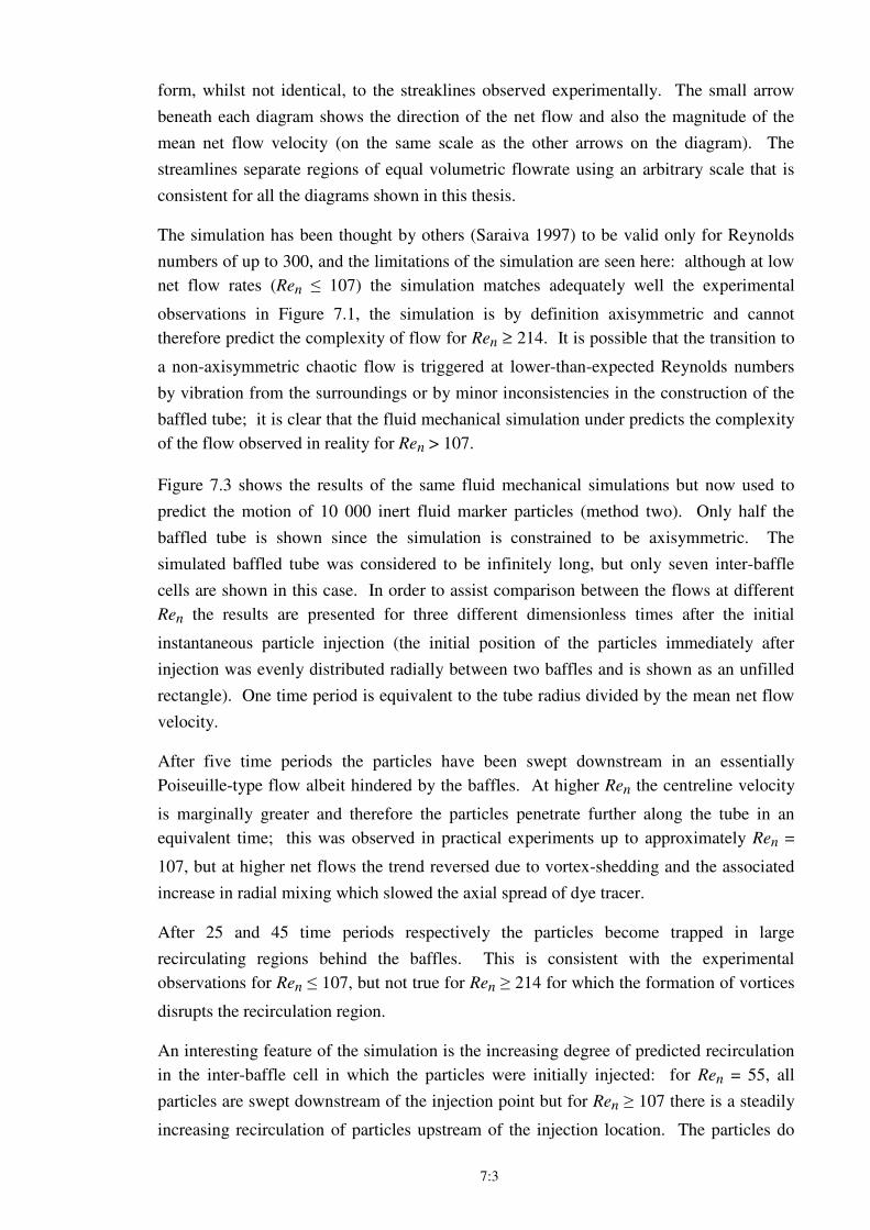
7:3
form, whilst not identical, to the streaklines observed experimentally. The small arrow
beneath each diagram shows the direction of the net flow and also the magnitude of the
mean net flow velocity (on the same scale as the other arrows on the diagram). The
streamlines separate regions of equal volumetric flowrate using an arbitrary scale that is
consistent for all the diagrams shown in this thesis.
The simulation has been thought by others (Saraiva 1997) to be valid only for Reynolds
numbers of up to 300, and the limitations of the simulation are seen here: although at low
net flow rates (Ren ≤ 107) the simulation matches adequately well the experimental
observations in Figure 7.1, the simulation is by definition axisymmetric and cannot
therefore predict the complexity of flow for Ren ≥ 214. It is possible that the transition to
a non-axisymmetric chaotic flow is triggered at lower-than-expected Reynolds numbers
by vibration from the surroundings or by minor inconsistencies in the construction of the
baffled tube; it is clear that the fluid mechanical simulation under predicts the complexity
of the flow observed in reality for Ren > 107.
Figure 7.3 shows the results of the same fluid mechanical simulations but now used to
predict the motion of 10 000 inert fluid marker particles (method two). Only half the
baffled tube is shown since the simulation is constrained to be axisymmetric. The
simulated baffled tube was considered to be infinitely long, but only seven inter-baffle
cells are shown in this case. In order to assist comparison between the flows at different
Ren the results are presented for three different dimensionless times after the initial
instantaneous particle injection (the initial position of the particles immediately after
injection was evenly distributed radially between two baffles and is shown as an unfilled
rectangle). One time period is equivalent to the tube radius divided by the mean net flow
velocity.
After five time periods the particles have been swept downstream in an essentially
Poiseuille-type flow albeit hindered by the baffles. At higher Ren the centreline velocity
is marginally greater and therefore the particles penetrate further along the tube in an
equivalent time; this was observed in practical experiments up to approximately Ren =
107, but at higher net flows the trend reversed due to vortex-shedding and the associated
increase in radial mixing which slowed the axial spread of dye tracer.
After 25 and 45 time periods respectively the particles become trapped in large
recirculating regions behind the baffles. This is consistent with the experimental
observations for Ren ≤ 107, but not true for Ren ≥ 214 for which the formation of vortices
disrupts the recirculation region.
An interesting feature of the simulation is the increasing degree of predicted recirculation
in the inter-baffle cell in which the particles were initially injected: for Ren = 55, all
particles are swept downstream of the injection point but for Ren ≥ 107 there is a steadily
increasing recirculation of particles upstream of the injection location. The particles do
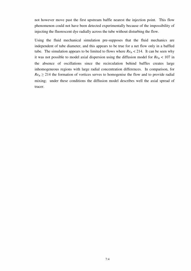
7:4
not however move past the first upstream baffle nearest the injection point. This flow
phenomenon could not have been detected experimentally because of the impossibility of
injecting the fluorescent dye radially across the tube without disturbing the flow.
Using the fluid mechanical simulation pre-supposes that the fluid mechanics are
independent of tube diameter, and this appears to be true for a net flow only in a baffled
tube. The simulation appears to be limited to flows where Ren < 214. It can be seen why
it was not possible to model axial dispersion using the diffusion model for Ren < 107 in
the absence of oscillations since the recirculation behind baffles creates large
inhomogeneous regions with large radial concentration differences. In comparison, for
Ren ≥ 214 the formation of vortices serves to homogenise the flow and to provide radial
mixing; under these conditions the diffusion model describes well the axial spread of
tracer.
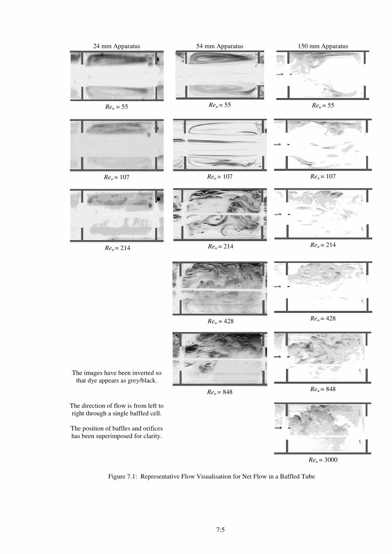
7:5
24 mm Apparatus 54 mm Apparatus 150 mm Apparatus
Ren = 55
Ren = 55
Ren = 55
Ren = 107
Ren = 107
Ren = 107
Ren = 214
Ren = 214
Ren = 214
Ren = 428
Ren = 428
The images have been inverted so
that dye appears as grey/black.
Ren = 848
Ren = 848
The direction of flow is from left to
right through a single baffled cell.
The position of baffles and orifices
has been superimposed for clarity.
Ren = 3000
Figure 7.1: Representative Flow Visualisation for Net Flow in a Baffled Tube
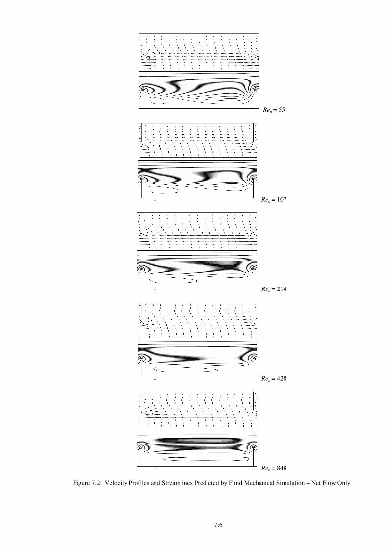
7:6
Ren = 55
Ren = 107
Ren = 214
Ren = 428
Ren = 848
Figure 7.2: Velocity Profiles and Streamlines Predicted by Fluid Mechanical Simulation – Net Flow Only
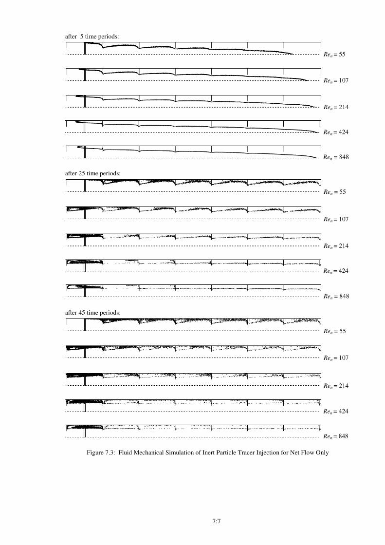
7:7
after 5 time periods:
Ren = 55
Ren = 107
Ren = 214
Ren = 424
Ren = 848 after 25 time periods:
Ren = 55
Ren = 107
Ren = 214
Ren = 424
Ren = 848 after 45 time periods:
Ren = 55
Ren = 107
Ren = 214
Ren = 424
Ren = 848
Figure 7.3: Fluid Mechanical Simulation of Inert Particle Tracer Injection for Net Flow Only
7:8
7.2 Flow Visualisation - Oscillation with No Net Flow
One of the very first flow visualisation experiments performed as part of this thesis was
without the benefit of the fluorescent dye technique but simply with the injection of
methylene blue dye into the 24 mm baffled tube with a modest oscillation of 0.3 Hz and 1
mm amplitude. The result was quite striking: after the initial disturbance of the dye
injection, a flow structure developed in the inter-baffle cell next to the injection point
which created a sharp divide of dye concentration across the middle of the inter-baffle
cell. Only gradually then did the dye seep into the other half of the cell by the formation
of lobes close to the tube wall and by diffusion across the divide. This type of flow
boundary has been termed "manifold" (Figure 7.4). Even after 30 minutes, the manifold is
clearly in evidence as a sharp concentration-divide between the two halves of the inter-
baffle cell. The manifold is formed by the interaction of axisymmetric vortices travelling
in opposite directions and which meet midway between two baffles. The vortices have
the same sense of rotation which sweeps elements of fluid from the centre of the tube
towards the wall and this creates a separation between the two halves of the inter-baffle
cell: because the velocity is primarily radial where the opposing vortices meet, negligible
tracer crosses the manifold axially by advection. The manifold moves a small distance up
and down with the fluid oscillation, but remains flat except for close to the tube wall
where the no-slip condition can generate folds or “lobes” in the manifold due to the
oscillations.
The existence and behaviour of these manifolds could be successfully predicted using the
fluid mechanical simulation: Figure 7.5 shows a direct comparison between simulation
and experiment for Reo = 75 and Str = 4 in the 54 mm apparatus. Using the fluorescent
streakline technique allows the "onion-peel" or “lamella” flow structure that creates the
manifolds to be seen, and as a result of uneven dye injection the dye is only present on the
left-hand half of the tube despite being well mixed. This is strong evidence that there is
minimal toroidal motion of the fluid under the flow conditions that created the manifolds.
The manifolds act as a barrier to axial dispersion whilst at the same time the oscillations
create relatively good stretch-fold mixing in the regions separated by the manifolds.
Where such manifolds are present, the axial diffusion model is a poor physical model for
dispersion over short distances in the baffled tube.
Only very delicately controlled oscillatory conditions allow the manifolds to exist. At the
same oscillatory Reynolds number to the previous example but with a larger amplitude
oscillation (Str = 2), Figure 7.6 (a) shows the resulting experimental streaklines: the
axisymmetry of the manifold is broken and although the manifold still exists, axial mixing
is much more rapid as the lobes extend into the next inter-baffle cell. The streaklines are
shown at four equally spaced times during one complete cycle of the oscillation and are
compared with predicted velocity profiles using the fluid mechanical simulation (b) for
which the simulation does not predict the asymmetry of the flow. Figure 7.6 (c) shows
7:9
simulation predictions of the movement of marker particles under these flow conditions;
again, the rate of axial mixing is underpredicted. A feature of the manifolds observed
both in experiment and in simulation is that depending upon the exact moment of dye
injection, dye injected equidistantly between two baffles will normally move
predominantly to either one side or the other of the injection point, i.e. the dye is not
distributed evenly each side of the injection point. This explains the apparent asymmetry
in readings from concentration measurements made equal distances either side of the
injection point at low oscillatory Reynolds numbers noted in §5.2 (Figure 5.13).
Figure 7.7 shows similar results but for a more rapid oscillation: while the simulation still
predicts the formation of manifolds, the experimental reality is quite different with
asymmetric flow, although the flow around the baffle orifice is similar in form to
simulation with large amounts of stretching and folding occurring in successive
oscillations.
The same experimental streaklines for the 54 mm apparatus shown in Figure 7.7 are
displayed again in Figure 7.8 but this time as a comparison of the observed flow in each
of the 24 mm, 54 mm and 150 mm sets of apparatus under similar dynamic conditions at
four separate times during a single oscillatory cycle. For each stage in the cycle, the flow
shows a similar distribution of vortices and vortex-sizes in the inter-baffle cell. The 54
mm apparatus shows a slightly higher degree of asymmetry in the flow, for which there is
no obvious cause other than the possibility of slight baffle eccentricity or of a disturbance
to the flow due to the method of dye injection in that particular apparatus.
The flow patterns observed for these conditions and a range of other values of Reo and
Str were generally similar enough in the three sets of apparatus to be able to conclude that
the flow is not substantially affected by tube diameter in this mixing regime. At much
higher Reynolds numbers (Reo > 800), the flow becomes sufficiently chaotic and
turbulent in nature that it is not possible to distinguish specific flow patterns, but rather
the measurements of other properties such as axial dispersion must be used to draw the
conclusion that fluid mechanics are not affected by tube diameter in the range studied.
Similarly to the case of net flow only, it has been found that the numerical simulation
underpredicts the complexity of the flow even for oscillatory Reynolds numbers as low as
75.
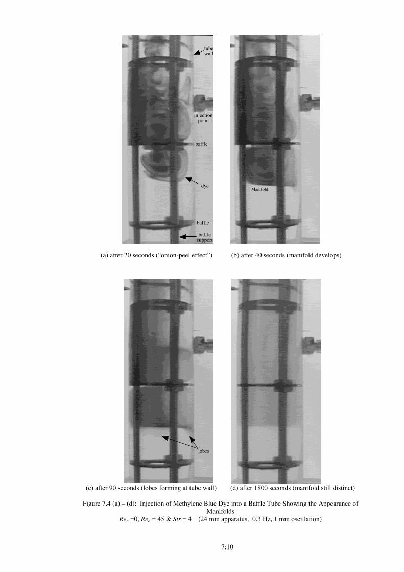
7:10
baffle
baffle
injection point
dye
baffle support
tube wall
Manifold
(a) after 20 seconds (“onion-peel effect”) (b) after 40 seconds (manifold develops)
lobes
(c) after 90 seconds (lobes forming at tube wall) (d) after 1800 seconds (manifold still distinct)
Figure 7.4 (a) – (d): Injection of Methylene Blue Dye into a Baffle Tube Showing the Appearance of
Manifolds
Ren =0, Reo = 45 & Str = 4 (24 mm apparatus, 0.3 Hz, 1 mm oscillation)
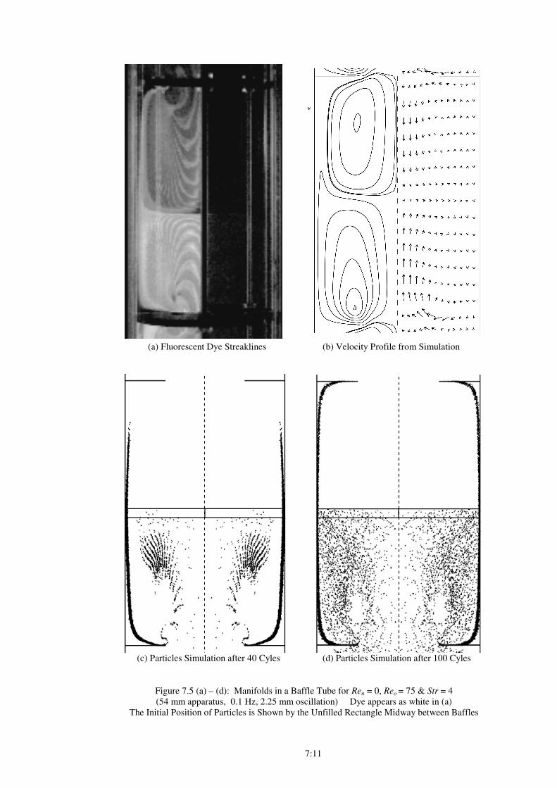
7:11
(a) Fluorescent Dye Streaklines (b) Velocity Profile from Simulation
(c) Particles Simulation after 40 Cyles (d) Particles Simulation after 100 Cyles
Figure 7.5 (a) – (d): Manifolds in a Baffle Tube for Ren = 0, Reo = 75 & Str = 4
(54 mm apparatus, 0.1 Hz, 2.25 mm oscillation) Dye appears as white in (a)
The Initial Position of Particles is Shown by the Unfilled Rectangle Midway between Baffles
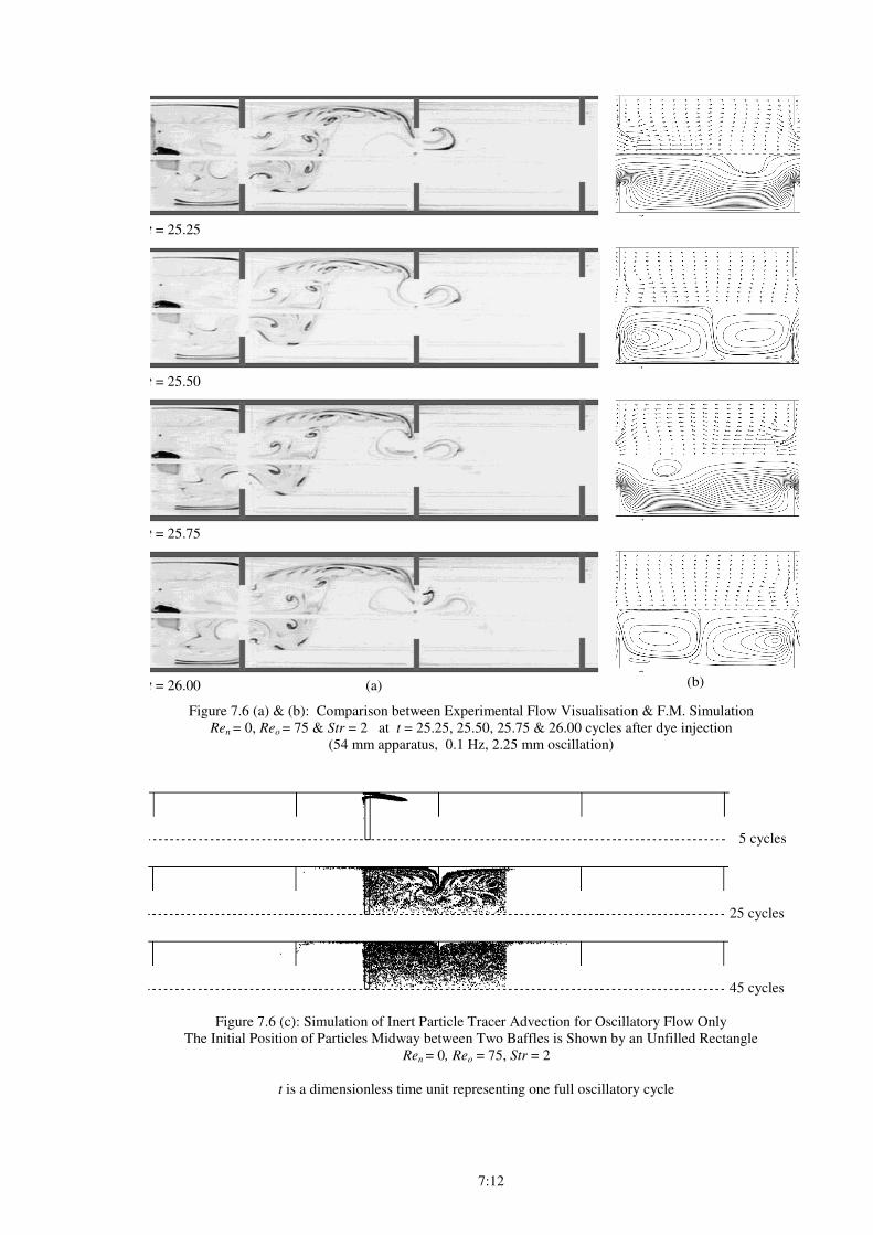
7:12
t = 25.25
t = 25.50
t = 25.75
t = 26.00 (a)
(b)
Figure 7.6 (a) & (b): Comparison between Experimental Flow Visualisation & F.M. Simulation
Ren = 0, Reo = 75 & Str = 2 at t = 25.25, 25.50, 25.75 & 26.00 cycles after dye injection
(54 mm apparatus, 0.1 Hz, 2.25 mm oscillation)
5 cycles
25 cycles
45 cycles
Figure 7.6 (c): Simulation of Inert Particle Tracer Advection for Oscillatory Flow Only
The Initial Position of Particles Midway between Two Baffles is Shown by an Unfilled Rectangle
Ren = 0, Reo = 75, Str = 2
t is a dimensionless time unit representing one full oscillatory cycle
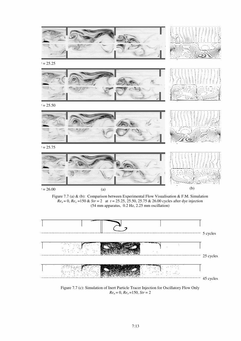
7:13
t = 25.25
t = 25.50
t = 25.75
t = 26.00 (a)
(b)
Figure 7.7 (a) & (b): Comparison between Experimental Flow Visualisation & F.M. Simulation
Ren = 0, Reo =150 & Str = 2 at t = 25.25, 25.50, 25.75 & 26.00 cycles after dye injection
(54 mm apparatus, 0.2 Hz, 2.25 mm oscillation)
5 cycles
25 cycles
45 cycles
Figure 7.7 (c): Simulation of Inert Particle Tracer Injection for Oscillatory Flow Only
Ren = 0, Reo =150, Str = 2
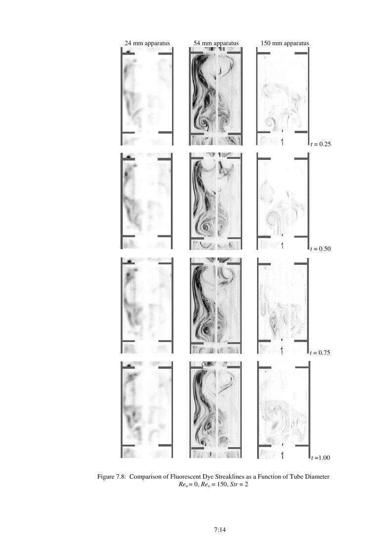
7:14
24 mm apparatus 54 mm apparatus 150 mm apparatus
t = 0.25
t = 0.50
t = 0.75
t =1.00
Figure 7.8: Comparison of Fluorescent Dye Streaklines as a Function of Tube Diameter
Ren = 0, Reo = 150, Str = 2
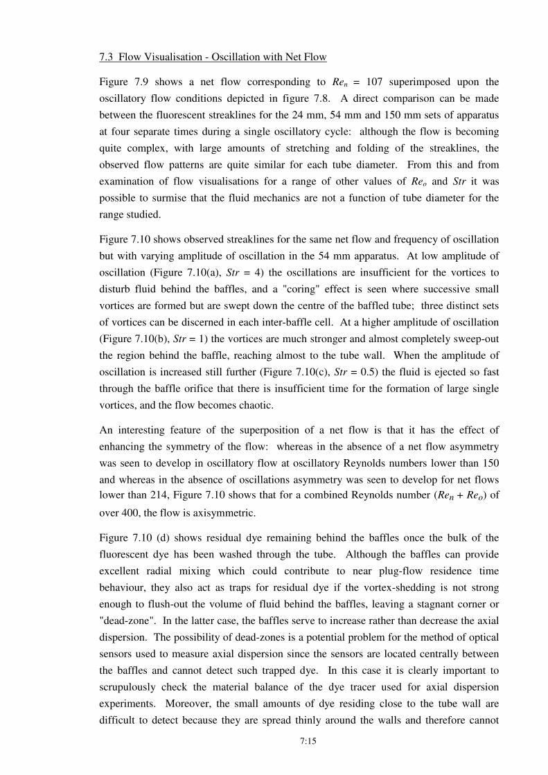
7:15
7.3 Flow Visualisation - Oscillation with Net Flow
Figure 7.9 shows a net flow corresponding to Ren = 107 superimposed upon the
oscillatory flow conditions depicted in figure 7.8. A direct comparison can be made
between the fluorescent streaklines for the 24 mm, 54 mm and 150 mm sets of apparatus
at four separate times during a single oscillatory cycle: although the flow is becoming
quite complex, with large amounts of stretching and folding of the streaklines, the
observed flow patterns are quite similar for each tube diameter. From this and from
examination of flow visualisations for a range of other values of Reo and Str it was
possible to surmise that the fluid mechanics are not a function of tube diameter for the
range studied.
Figure 7.10 shows observed streaklines for the same net flow and frequency of oscillation
but with varying amplitude of oscillation in the 54 mm apparatus. At low amplitude of
oscillation (Figure 7.10(a), Str = 4) the oscillations are insufficient for the vortices to
disturb fluid behind the baffles, and a "coring" effect is seen where successive small
vortices are formed but are swept down the centre of the baffled tube; three distinct sets
of vortices can be discerned in each inter-baffle cell. At a higher amplitude of oscillation
(Figure 7.10(b), Str = 1) the vortices are much stronger and almost completely sweep-out
the region behind the baffle, reaching almost to the tube wall. When the amplitude of
oscillation is increased still further (Figure 7.10(c), Str = 0.5) the fluid is ejected so fast
through the baffle orifice that there is insufficient time for the formation of large single
vortices, and the flow becomes chaotic.
An interesting feature of the superposition of a net flow is that it has the effect of
enhancing the symmetry of the flow: whereas in the absence of a net flow asymmetry
was seen to develop in oscillatory flow at oscillatory Reynolds numbers lower than 150
and whereas in the absence of oscillations asymmetry was seen to develop for net flows
lower than 214, Figure 7.10 shows that for a combined Reynolds number (Ren + Reo) of
over 400, the flow is axisymmetric.
Figure 7.10 (d) shows residual dye remaining behind the baffles once the bulk of the
fluorescent dye has been washed through the tube. Although the baffles can provide
excellent radial mixing which could contribute to near plug-flow residence time
behaviour, they also act as traps for residual dye if the vortex-shedding is not strong
enough to flush-out the volume of fluid behind the baffles, leaving a stagnant corner or
"dead-zone". In the latter case, the baffles serve to increase rather than decrease the axial
dispersion. The possibility of dead-zones is a potential problem for the method of optical
sensors used to measure axial dispersion since the sensors are located centrally between
the baffles and cannot detect such trapped dye. In this case it is clearly important to
scrupulously check the material balance of the dye tracer used for axial dispersion
experiments. Moreover, the small amounts of dye residing close to the tube wall are
difficult to detect because they are spread thinly around the walls and therefore cannot
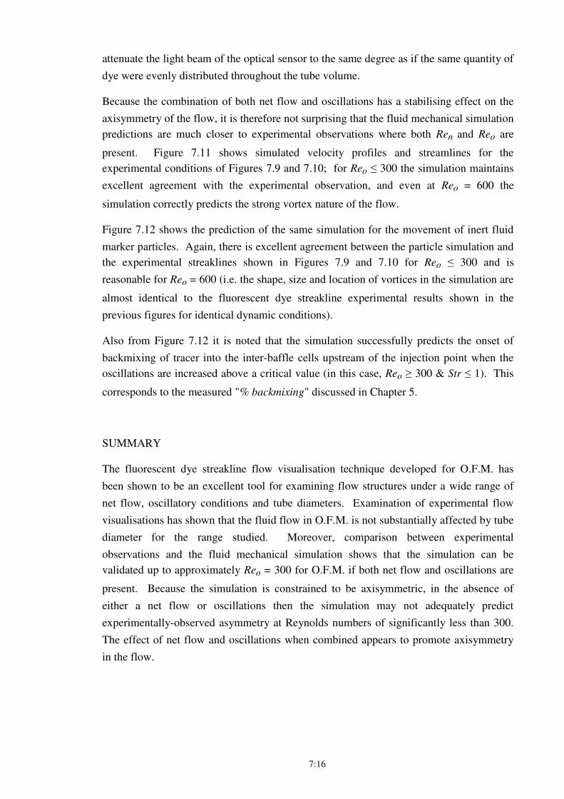
7:16
attenuate the light beam of the optical sensor to the same degree as if the same quantity of
dye were evenly distributed throughout the tube volume.
Because the combination of both net flow and oscillations has a stabilising effect on the
axisymmetry of the flow, it is therefore not surprising that the fluid mechanical simulation
predictions are much closer to experimental observations where both Ren and Reo are
present. Figure 7.11 shows simulated velocity profiles and streamlines for the
experimental conditions of Figures 7.9 and 7.10; for Reo ≤ 300 the simulation maintains
excellent agreement with the experimental observation, and even at Reo = 600 the
simulation correctly predicts the strong vortex nature of the flow.
Figure 7.12 shows the prediction of the same simulation for the movement of inert fluid
marker particles. Again, there is excellent agreement between the particle simulation and
the experimental streaklines shown in Figures 7.9 and 7.10 for Reo ≤ 300 and is
reasonable for Reo = 600 (i.e. the shape, size and location of vortices in the simulation are
almost identical to the fluorescent dye streakline experimental results shown in the
previous figures for identical dynamic conditions).
Also from Figure 7.12 it is noted that the simulation successfully predicts the onset of
backmixing of tracer into the inter-baffle cells upstream of the injection point when the
oscillations are increased above a critical value (in this case, Reo ≥ 300 & Str ≤ 1). This
corresponds to the measured "% backmixing" discussed in Chapter 5.
SUMMARY
The fluorescent dye streakline flow visualisation technique developed for O.F.M. has
been shown to be an excellent tool for examining flow structures under a wide range of
net flow, oscillatory conditions and tube diameters. Examination of experimental flow
visualisations has shown that the fluid flow in O.F.M. is not substantially affected by tube
diameter for the range studied. Moreover, comparison between experimental
observations and the fluid mechanical simulation shows that the simulation can be
validated up to approximately Reo = 300 for O.F.M. if both net flow and oscillations are
present. Because the simulation is constrained to be axisymmetric, in the absence of
either a net flow or oscillations then the simulation may not adequately predict
experimentally-observed asymmetry at Reynolds numbers of significantly less than 300.
The effect of net flow and oscillations when combined appears to promote axisymmetry
in the flow.
7:17
24 mm apparatus 54 mm apparatus 150 mm apparatus
t = 0.25
t = 0.50
t = 0.75
t = 1.00
Figure 7.9: Experimental Streaklines in O.F.M. as a Function of Tube Diameter
Ren = 107, Reo = 150, Str = 2
7:18
(a) Ren =107, Reo =75, Str =4 (b) Ren =107, Reo =300, Str =1 (c) Ren =107, Reo =600, Str =0.5
(d) Ren =107, Reo =150, Str =2 After 10 minutes Showing Dye Trapped in Stagnant Corners behind Baffles
Figure 7.10 (a) – (d): Fluorescent Streaklines for Various Conditions in the 54mm Apparatus with Ren
=107
Each Diagram Showing 2 Inter-Baffle Cells
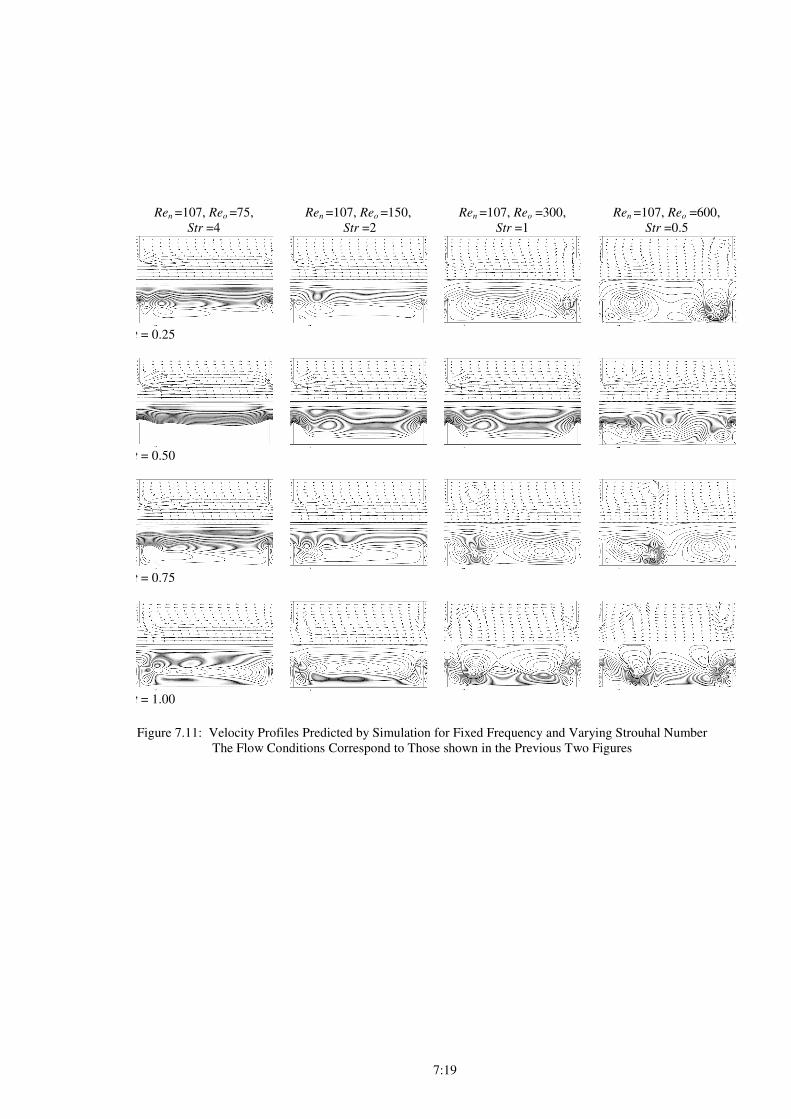
7:19
Ren =107, Reo =75,
Str =4
Ren =107, Reo =150,
Str =2
Ren =107, Reo =300,
Str =1
Ren =107, Reo =600,
Str =0.5
t = 0.25
t = 0.50
t = 0.75
t = 1.00
Figure 7.11: Velocity Profiles Predicted by Simulation for Fixed Frequency and Varying Strouhal Number
The Flow Conditions Correspond to Those shown in the Previous Two Figures
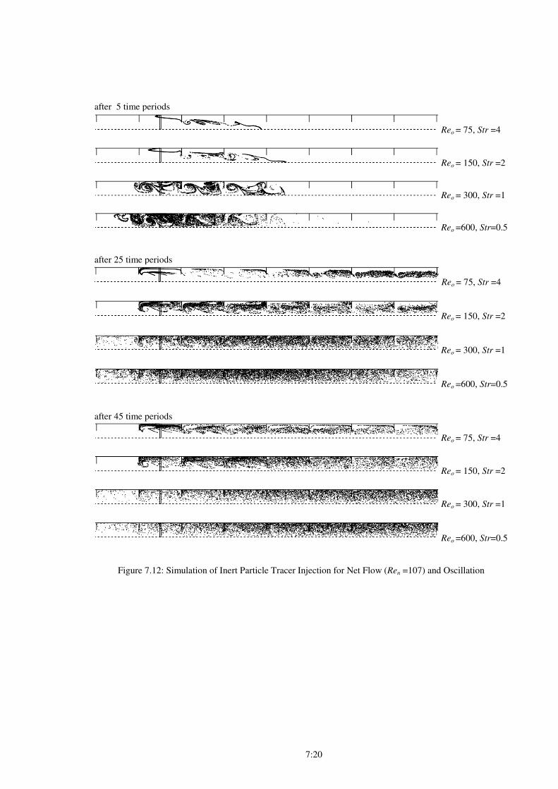
7:20
after 5 time periods
Reo = 75, Str =4
Reo = 150, Str =2
Reo = 300, Str =1
Reo =600, Str=0.5
after 25 time periods
Reo = 75, Str =4
Reo = 150, Str =2
Reo = 300, Str =1
Reo =600, Str=0.5
after 45 time periods
Reo = 75, Str =4
Reo = 150, Str =2
Reo = 300, Str =1
Reo =600, Str=0.5
Figure 7.12: Simulation of Inert Particle Tracer Injection for Net Flow (Ren =107) and Oscillation
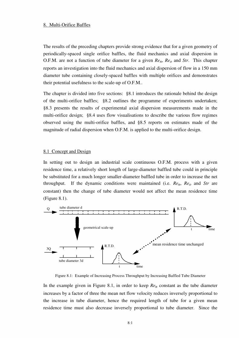
8:1
8. Multi-Orifice Baffles
The results of the preceding chapters provide strong evidence that for a given geometry of
periodically-spaced single orifice baffles, the fluid mechanics and axial dispersion in
O.F.M. are not a function of tube diameter for a given Ren, Reo and Str. This chapter
reports an investigation into the fluid mechanics and axial dispersion of flow in a 150 mm
diameter tube containing closely-spaced baffles with multiple orifices and demonstrates
their potential usefulness to the scale-up of O.F.M..
The chapter is divided into five sections: §8.1 introduces the rationale behind the design
of the multi-orifice baffles; §8.2 outlines the programme of experiments undertaken;
§8.3 presents the results of experimental axial dispersion measurements made in the
multi-orifice design; §8.4 uses flow visualisations to describe the various flow regimes
observed using the multi-orifice baffles, and §8.5 reports on estimates made of the
magnitude of radial dispersion when O.F.M. is applied to the multi-orifice design.
8.1 Concept and Design
In setting out to design an industrial scale continuous O.F.M. process with a given
residence time, a relatively short length of large-diameter baffled tube could in principle
be substituted for a much longer smaller-diameter baffled tube in order to increase the net
throughput. If the dynamic conditions were maintained (i.e. Ren, Reo and Str are
constant) then the change of tube diameter would not affect the mean residence time
(Figure 8.1).
Figure 8.1: Example of Increasing Process Throughput by Increasing Baffled Tube Diameter
In the example given in Figure 8.1, in order to keep Ren constant as the tube diameter
increases by a factor of three the mean net flow velocity reduces inversely proportional to
the increase in tube diameter, hence the required length of tube for a given mean
residence time must also decrease inversely proportional to tube diameter. Since the
time
R.T.D.tube diameter d
tube diameter 3d
geometrical scale-up
time
R.T.D.
t
t
residence time & distribution
remain unchanged
Q
3Q
residence time unchangedmean residence time unchanged
8:2
volume of the tube increases by length x (diameter)2, the throughput of the process would
increase by a factor of three. The absolute magnitude of the axial dispersion coefficient
remains constant regardless of tube diameter, therefore if the axial dispersion has been
measured for the smaller diameter tube then the residence time distribution for the larger
diameter tube can be calculated from, for example, equation (2.17).
Increasing the diameter of the tube is therefore an effective method for scaling-up O.F.M.
if residence time and residence time distribution are the only objectives. However, it is
most likely that some degree of fluid agitation/mixing and or wall heat transfer will be
required for an industrial process and it is then that simple geometrical scaling of O.F.M.
becomes problematic. As previously discussed in Chapter 3, in order to maintain
dynamic similarity of the flow conditions as the tube diameter increases the peak mean
velocity of oscillation is required to decrease inversely-proportional to tube diameter.
This means that the likely maximum shear-rates experienced by the fluid will decrease as
the inverse-square of the increase in tube diameter (assuming that the typical shear rates
will be related to a characteristic velocity divided by a characteristic length scale). This
in turn implies that micro mixing of the fluid will become very poor as tube diameter is
increased because the oscillations are very slow. Even for the relatively modest tube
diameter of 150 mm the required period of oscillation can be of order minutes rather than
seconds if the optimum conditions to minimise axial dispersion are sought, meaning very
slow fluid mixing and extremely poor wall heat transfer. In the latter case, convective
heat transfer would likely dominate any forced heat transfer and would probably change
the fluid mechanics of the system. (If however neither rapid mixing nor wall heat transfer
were necessary to the process then geometrical scaling could be very attractive since the
pressure drops and hence oscillator power requirements would be minimal).
An alternative solution to geometrical scaling-up of O.F.M. was proposed by Ni (1994)
who operated several 24 mm diameter tubes in parallel. This method has the advantages
of predictable fluid mechanics and good heat-transfer capabilities, although a potentially
vast number of individual tubes would be required for a large throughput process and
there are potential issues of distributing feed and oscillations evenly to each tube.
An alternative approach to the scale-up of O.F.M. was adopted in this thesis: instead of
having many small diameter tubes operating in parallel, the concept of a single large-
diameter tube containing closely-spaced baffles each with many orifices was developed
(see Figure 8.2). The design therefore mimics the effect of many smaller diameter tubes
in parallel and appears similar to a reciprocating plate column (except that the fluid is
oscillated and not the baffles). The predicted advantage of the multi-orifice baffles in the
150 mm diameter tube is that the same shear-rates and intensity of mixing can be
achieved as in the 24 mm diameter tube while greatly increasing the throughput of the
process. In order to achieve the same shear rates, residence time and residence time
distribution then the length of the multi-orifice 150 mm diameter tube would be the same
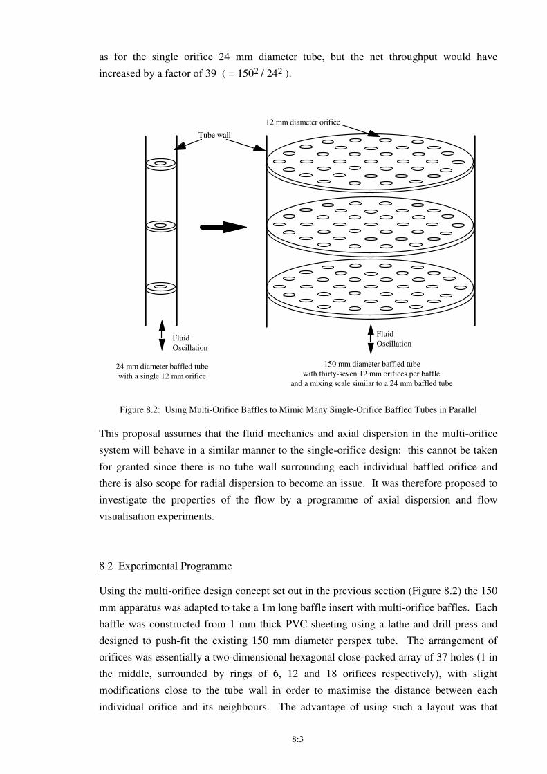
8:3
as for the single orifice 24 mm diameter tube, but the net throughput would have
increased by a factor of 39 ( = 1502 / 242 ).
Fluid
Oscillation
24 mm diameter baffled tube
with a single 12 mm orifice
150 mm diameter baffled tube
with thirty-seven 12 mm orifices per baffle
and a mixing scale similar to a 24 mm baffled tube
Fluid
Oscillation
Tube wall
12 mm diameter orifice
Figure 8.2: Using Multi-Orifice Baffles to Mimic Many Single-Orifice Baffled Tubes in Parallel
This proposal assumes that the fluid mechanics and axial dispersion in the multi-orifice
system will behave in a similar manner to the single-orifice design: this cannot be taken
for granted since there is no tube wall surrounding each individual baffled orifice and
there is also scope for radial dispersion to become an issue. It was therefore proposed to
investigate the properties of the flow by a programme of axial dispersion and flow
visualisation experiments.
8.2 Experimental Programme
Using the multi-orifice design concept set out in the previous section (Figure 8.2) the 150
mm apparatus was adapted to take a 1m long baffle insert with multi-orifice baffles. Each
baffle was constructed from 1 mm thick PVC sheeting using a lathe and drill press and
designed to push-fit the existing 150 mm diameter perspex tube. The arrangement of
orifices was essentially a two-dimensional hexagonal close-packed array of 37 holes (1 in
the middle, surrounded by rings of 6, 12 and 18 orifices respectively), with slight
modifications close to the tube wall in order to maximise the distance between each
individual orifice and its neighbours. The advantage of using such a layout was that
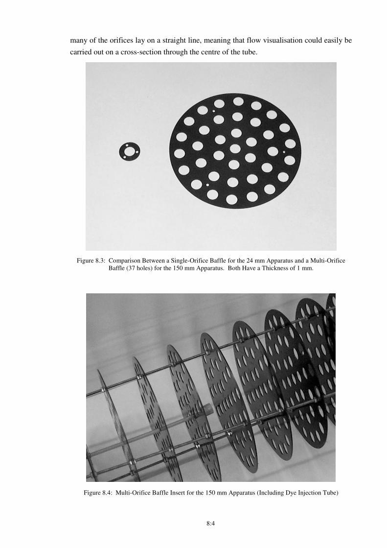
8:4
many of the orifices lay on a straight line, meaning that flow visualisation could easily be
carried out on a cross-section through the centre of the tube.
Figure 8.3: Comparison Between a Single-Orifice Baffle for the 24 mm Apparatus and a Multi-Orifice
Baffle (37 holes) for the 150 mm Apparatus. Both Have a Thickness of 1 mm.
Figure 8.4: Multi-Orifice Baffle Insert for the 150 mm Apparatus (Including Dye Injection Tube)
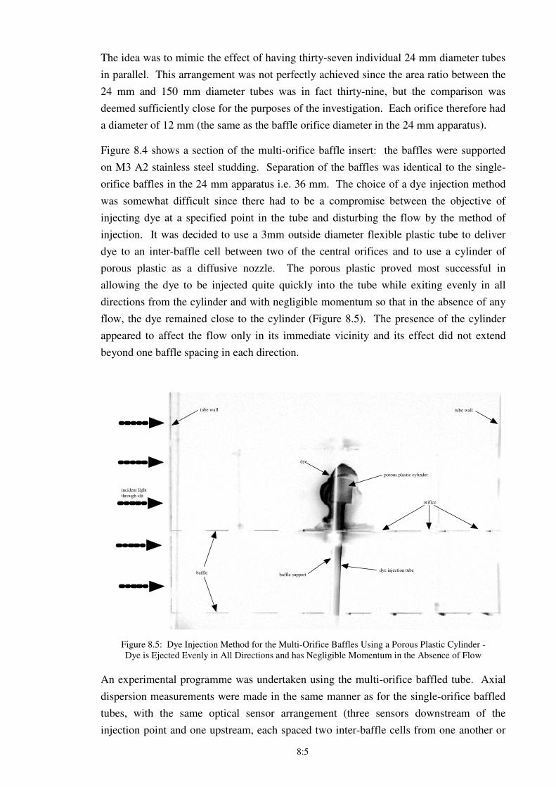
8:5
The idea was to mimic the effect of having thirty-seven individual 24 mm diameter tubes
in parallel. This arrangement was not perfectly achieved since the area ratio between the
24 mm and 150 mm diameter tubes was in fact thirty-nine, but the comparison was
deemed sufficiently close for the purposes of the investigation. Each orifice therefore had
a diameter of 12 mm (the same as the baffle orifice diameter in the 24 mm apparatus).
Figure 8.4 shows a section of the multi-orifice baffle insert: the baffles were supported
on M3 A2 stainless steel studding. Separation of the baffles was identical to the single-
orifice baffles in the 24 mm apparatus i.e. 36 mm. The choice of a dye injection method
was somewhat difficult since there had to be a compromise between the objective of
injecting dye at a specified point in the tube and disturbing the flow by the method of
injection. It was decided to use a 3mm outside diameter flexible plastic tube to deliver
dye to an inter-baffle cell between two of the central orifices and to use a cylinder of
porous plastic as a diffusive nozzle. The porous plastic proved most successful in
allowing the dye to be injected quite quickly into the tube while exiting evenly in all
directions from the cylinder and with negligible momentum so that in the absence of any
flow, the dye remained close to the cylinder (Figure 8.5). The presence of the cylinder
appeared to affect the flow only in its immediate vicinity and its effect did not extend
beyond one baffle spacing in each direction.
tube wall tube wall
baffle baffle supportdye injection tube
orifice
dye
porous plastic cylinder
incident light
through slit
Figure 8.5: Dye Injection Method for the Multi-Orifice Baffles Using a Porous Plastic Cylinder -
Dye is Ejected Evenly in All Directions and has Negligible Momentum in the Absence of Flow
An experimental programme was undertaken using the multi-orifice baffled tube. Axial
dispersion measurements were made in the same manner as for the single-orifice baffled
tubes, with the same optical sensor arrangement (three sensors downstream of the
injection point and one upstream, each spaced two inter-baffle cells from one another or
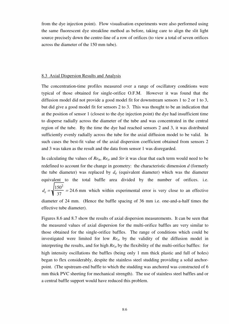
8:6
from the dye injection point). Flow visualisation experiments were also performed using
the same fluorescent dye streakline method as before, taking care to align the slit light
source precisely down the centre-line of a row of orifices (to view a total of seven orifices
across the diameter of the 150 mm tube).
8.3 Axial Dispersion Results and Analysis
The concentration-time profiles measured over a range of oscillatory conditions were
typical of those obtained for single-orifice O.F.M. However it was found that the
diffusion model did not provide a good model fit for downstream sensors 1 to 2 or 1 to 3,
but did give a good model fit for sensors 2 to 3. This was thought to be an indication that
at the position of sensor 1 (closest to the dye injection point) the dye had insufficient time
to disperse radially across the diameter of the tube and was concentrated in the central
region of the tube. By the time the dye had reached sensors 2 and 3, it was distributed
sufficiently evenly radially across the tube for the axial diffusion model to be valid. In
such cases the best-fit value of the axial dispersion coefficient obtained from sensors 2
and 3 was taken as the result and the data from sensor 1 was disregarded.
In calculating the values of Ren, Reo and Str it was clear that each term would need to be
redefined to account for the change in geometry: the characteristic dimension d (formerly
the tube diameter) was replaced by de (equivalent diameter) which was the diameter
equivalent to the total baffle area divided by the number of orifices. i.e.
de =
1502
37= 24.6 mm which within experimental error is very close to an effective
diameter of 24 mm. (Hence the baffle spacing of 36 mm i.e. one-and-a-half times the
effective tube diameter).
Figures 8.6 and 8.7 show the results of axial dispersion measurements. It can be seen that
the measured values of axial dispersion for the multi-orifice baffles are very similar to
those obtained for the single-orifice baffles. The range of conditions which could be
investigated were limited for low Reo by the validity of the diffusion model in
interpreting the results, and for high Reo by the flexibility of the multi-orifice baffles: for
high intensity oscillations the baffles (being only 1 mm thick plastic and full of holes)
began to flex considerably, despite the stainless steel studding providing a solid anchor-
point. (The upstream-end baffle to which the studding was anchored was constructed of 6
mm thick PVC sheeting for mechanical strength). The use of stainless steel baffles and or
a central baffle support would have reduced this problem.
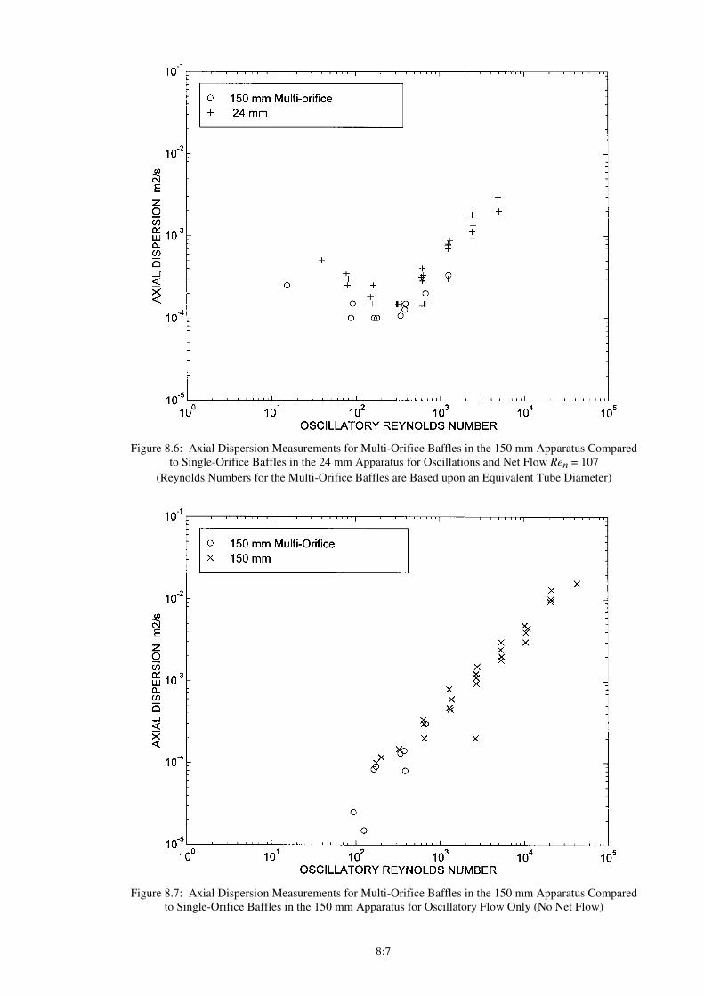
8:7
Figure 8.6: Axial Dispersion Measurements for Multi-Orifice Baffles in the 150 mm Apparatus Compared
to Single-Orifice Baffles in the 24 mm Apparatus for Oscillations and Net Flow Ren = 107
(Reynolds Numbers for the Multi-Orifice Baffles are Based upon an Equivalent Tube Diameter)
Figure 8.7: Axial Dispersion Measurements for Multi-Orifice Baffles in the 150 mm Apparatus Compared
to Single-Orifice Baffles in the 150 mm Apparatus for Oscillatory Flow Only (No Net Flow)
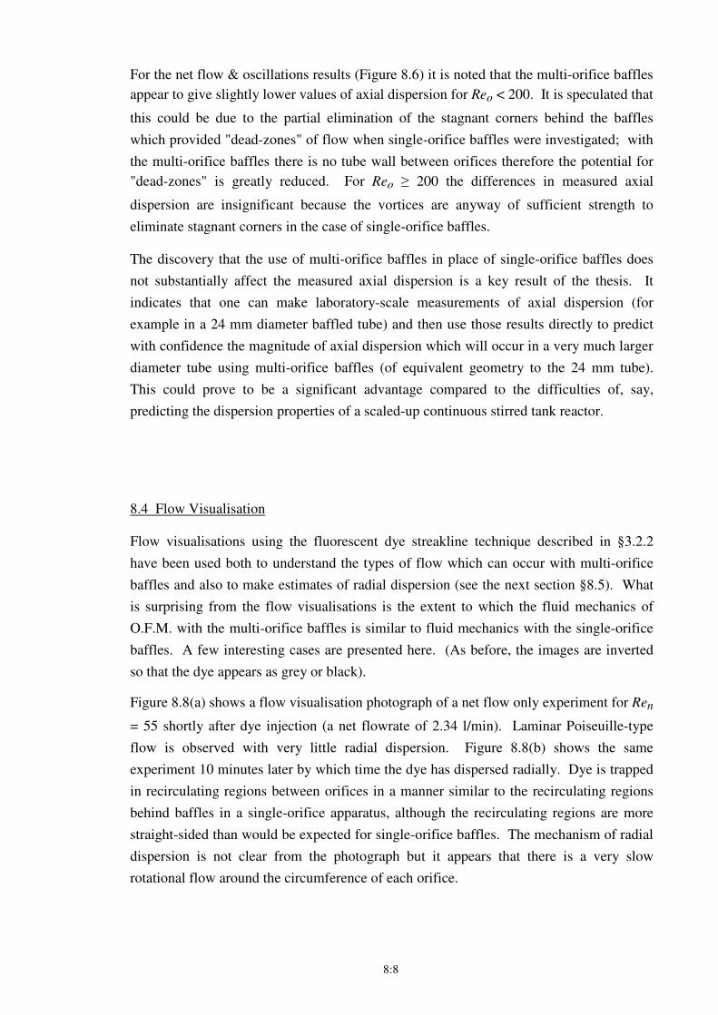
8:8
For the net flow & oscillations results (Figure 8.6) it is noted that the multi-orifice baffles
appear to give slightly lower values of axial dispersion for Reo < 200. It is speculated that
this could be due to the partial elimination of the stagnant corners behind the baffles
which provided "dead-zones" of flow when single-orifice baffles were investigated; with
the multi-orifice baffles there is no tube wall between orifices therefore the potential for
"dead-zones" is greatly reduced. For Reo ≥ 200 the differences in measured axial
dispersion are insignificant because the vortices are anyway of sufficient strength to
eliminate stagnant corners in the case of single-orifice baffles.
The discovery that the use of multi-orifice baffles in place of single-orifice baffles does
not substantially affect the measured axial dispersion is a key result of the thesis. It
indicates that one can make laboratory-scale measurements of axial dispersion (for
example in a 24 mm diameter baffled tube) and then use those results directly to predict
with confidence the magnitude of axial dispersion which will occur in a very much larger
diameter tube using multi-orifice baffles (of equivalent geometry to the 24 mm tube).
This could prove to be a significant advantage compared to the difficulties of, say,
predicting the dispersion properties of a scaled-up continuous stirred tank reactor.
8.4 Flow Visualisation
Flow visualisations using the fluorescent dye streakline technique described in §3.2.2
have been used both to understand the types of flow which can occur with multi-orifice
baffles and also to make estimates of radial dispersion (see the next section §8.5). What
is surprising from the flow visualisations is the extent to which the fluid mechanics of
O.F.M. with the multi-orifice baffles is similar to fluid mechanics with the single-orifice
baffles. A few interesting cases are presented here. (As before, the images are inverted
so that the dye appears as grey or black).
Figure 8.8(a) shows a flow visualisation photograph of a net flow only experiment for Ren
= 55 shortly after dye injection (a net flowrate of 2.34 l/min). Laminar Poiseuille-type
flow is observed with very little radial dispersion. Figure 8.8(b) shows the same
experiment 10 minutes later by which time the dye has dispersed radially. Dye is trapped
in recirculating regions between orifices in a manner similar to the recirculating regions
behind baffles in a single-orifice apparatus, although the recirculating regions are more
straight-sided than would be expected for single-orifice baffles. The mechanism of radial
dispersion is not clear from the photograph but it appears that there is a very slow
rotational flow around the circumference of each orifice.
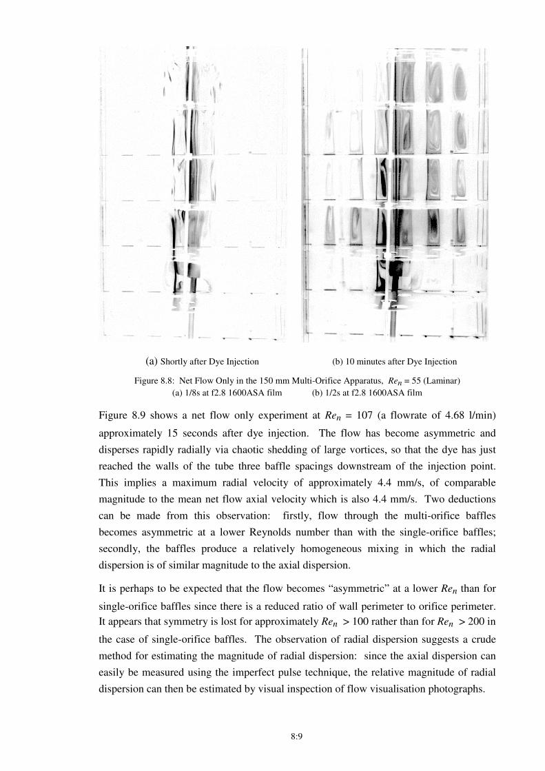
8:9
(a) Shortly after Dye Injection (b) 10 minutes after Dye Injection
Figure 8.8: Net Flow Only in the 150 mm Multi-Orifice Apparatus, Ren = 55 (Laminar)
(a) 1/8s at f2.8 1600ASA film (b) 1/2s at f2.8 1600ASA film
Figure 8.9 shows a net flow only experiment at Ren = 107 (a flowrate of 4.68 l/min)
approximately 15 seconds after dye injection. The flow has become asymmetric and
disperses rapidly radially via chaotic shedding of large vortices, so that the dye has just
reached the walls of the tube three baffle spacings downstream of the injection point.
This implies a maximum radial velocity of approximately 4.4 mm/s, of comparable
magnitude to the mean net flow axial velocity which is also 4.4 mm/s. Two deductions
can be made from this observation: firstly, flow through the multi-orifice baffles
becomes asymmetric at a lower Reynolds number than with the single-orifice baffles;
secondly, the baffles produce a relatively homogeneous mixing in which the radial
dispersion is of similar magnitude to the axial dispersion.
It is perhaps to be expected that the flow becomes “asymmetric” at a lower Ren than for
single-orifice baffles since there is a reduced ratio of wall perimeter to orifice perimeter.
It appears that symmetry is lost for approximately Ren > 100 rather than for Ren > 200 in
the case of single-orifice baffles. The observation of radial dispersion suggests a crude
method for estimating the magnitude of radial dispersion: since the axial dispersion can
easily be measured using the imperfect pulse technique, the relative magnitude of radial
dispersion can then be estimated by visual inspection of flow visualisation photographs.
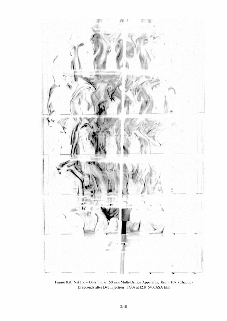
8:10
Figure 8.9: Net Flow Only in the 150 mm Multi-Orifice Apparatus, Ren = 107 (Chaotic)
15 seconds after Dye Injection 1/30s at f2.8 6400ASA film
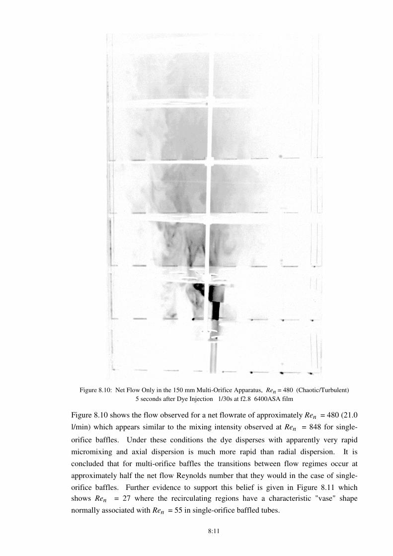
8:11
Figure 8.10: Net Flow Only in the 150 mm Multi-Orifice Apparatus, Ren = 480 (Chaotic/Turbulent)
5 seconds after Dye Injection 1/30s at f2.8 6400ASA film
Figure 8.10 shows the flow observed for a net flowrate of approximately Ren = 480 (21.0
l/min) which appears similar to the mixing intensity observed at Ren = 848 for single-
orifice baffles. Under these conditions the dye disperses with apparently very rapid
micromixing and axial dispersion is much more rapid than radial dispersion. It is
concluded that for multi-orifice baffles the transitions between flow regimes occur at
approximately half the net flow Reynolds number that they would in the case of single-
orifice baffles. Further evidence to support this belief is given in Figure 8.11 which
shows Ren = 27 where the recirculating regions have a characteristic "vase" shape
normally associated with Ren = 55 in single-orifice baffled tubes.
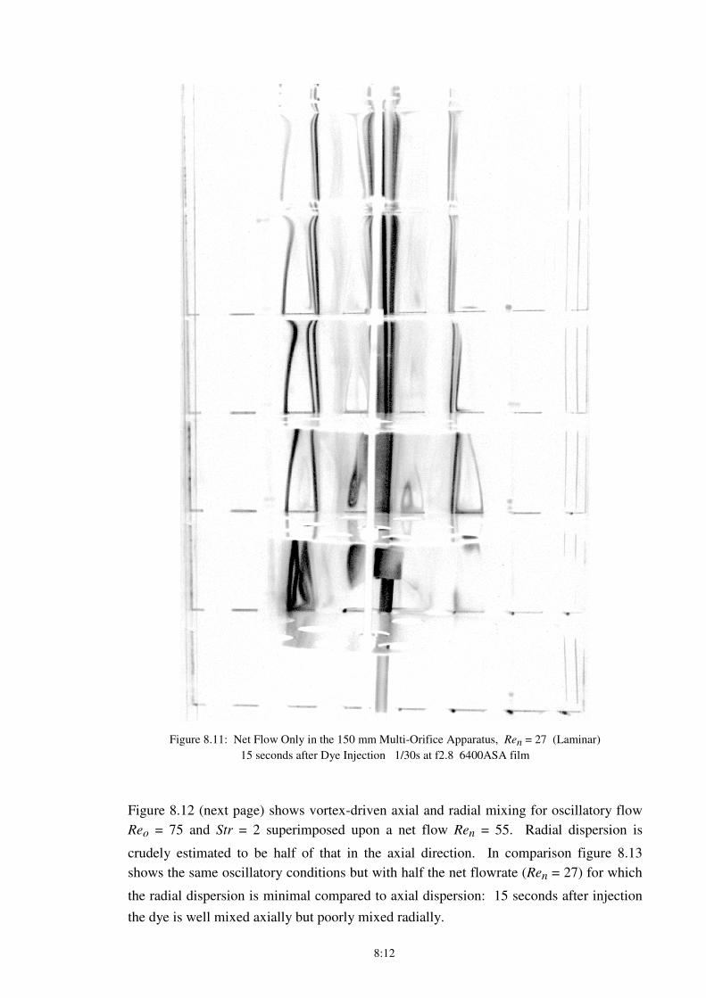
8:12
Figure 8.11: Net Flow Only in the 150 mm Multi-Orifice Apparatus, Ren = 27 (Laminar)
15 seconds after Dye Injection 1/30s at f2.8 6400ASA film
Figure 8.12 (next page) shows vortex-driven axial and radial mixing for oscillatory flow
Reo = 75 and Str = 2 superimposed upon a net flow Ren = 55. Radial dispersion is
crudely estimated to be half of that in the axial direction. In comparison figure 8.13
shows the same oscillatory conditions but with half the net flowrate (Ren = 27) for which
the radial dispersion is minimal compared to axial dispersion: 15 seconds after injection
the dye is well mixed axially but poorly mixed radially.
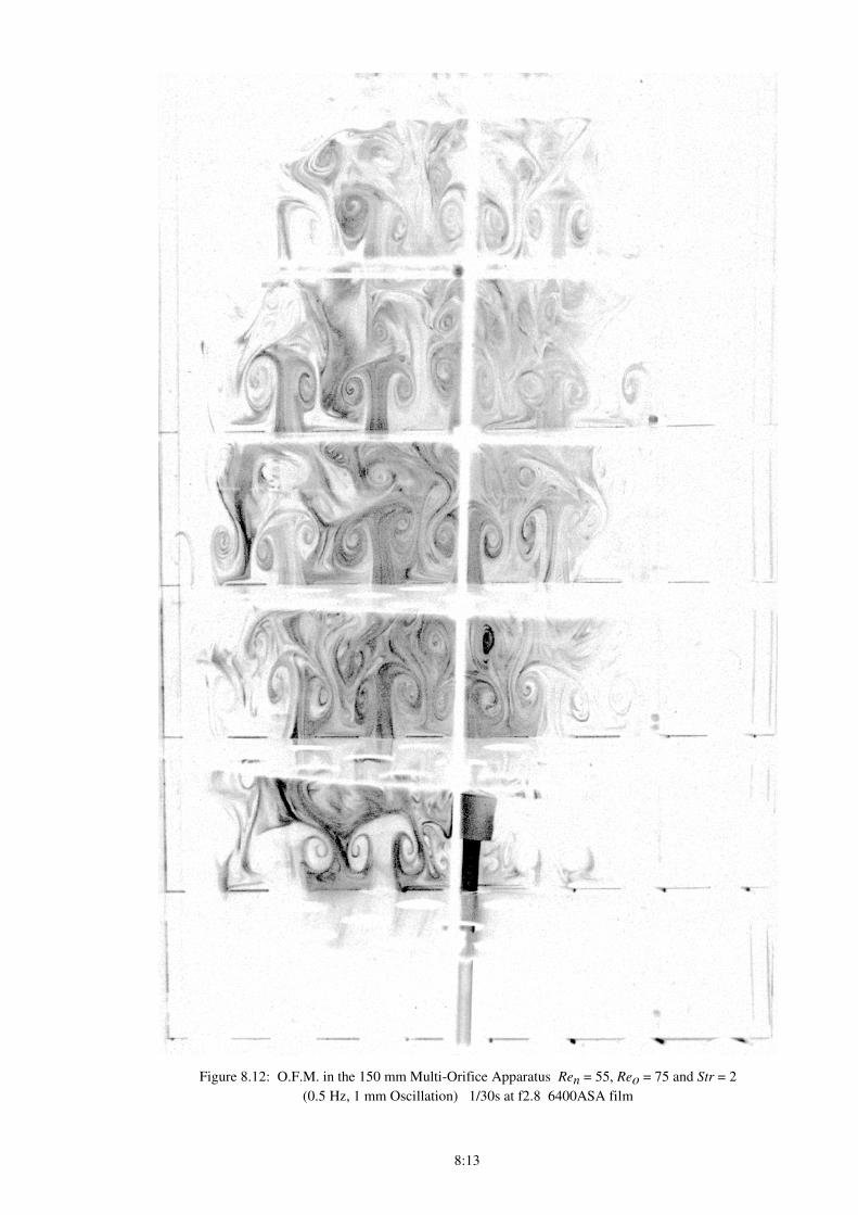
8:13
Figure 8.12: O.F.M. in the 150 mm Multi-Orifice Apparatus Ren = 55, Reo = 75 and Str = 2
(0.5 Hz, 1 mm Oscillation) 1/30s at f2.8 6400ASA film
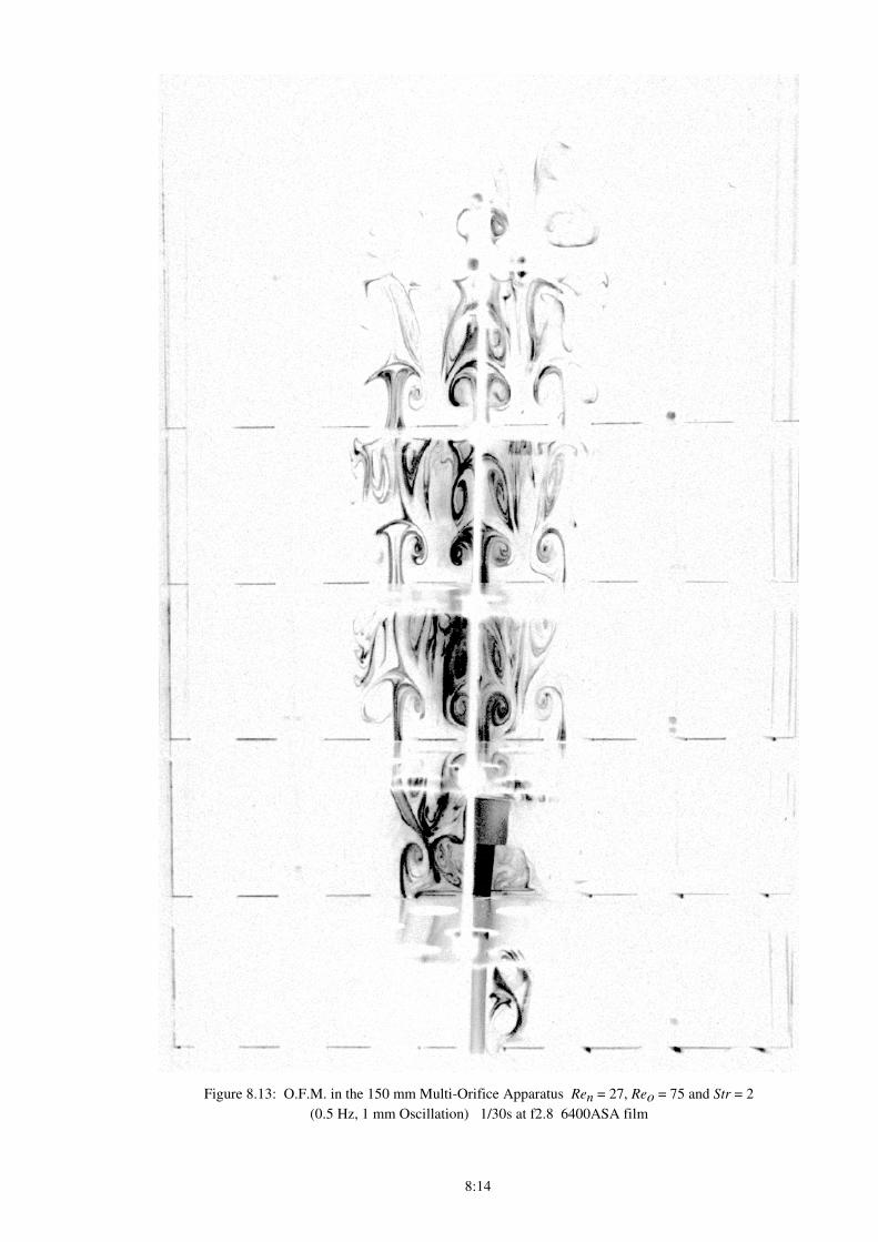
8:14
Figure 8.13: O.F.M. in the 150 mm Multi-Orifice Apparatus Ren = 27, Reo = 75 and Str = 2
(0.5 Hz, 1 mm Oscillation) 1/30s at f2.8 6400ASA film
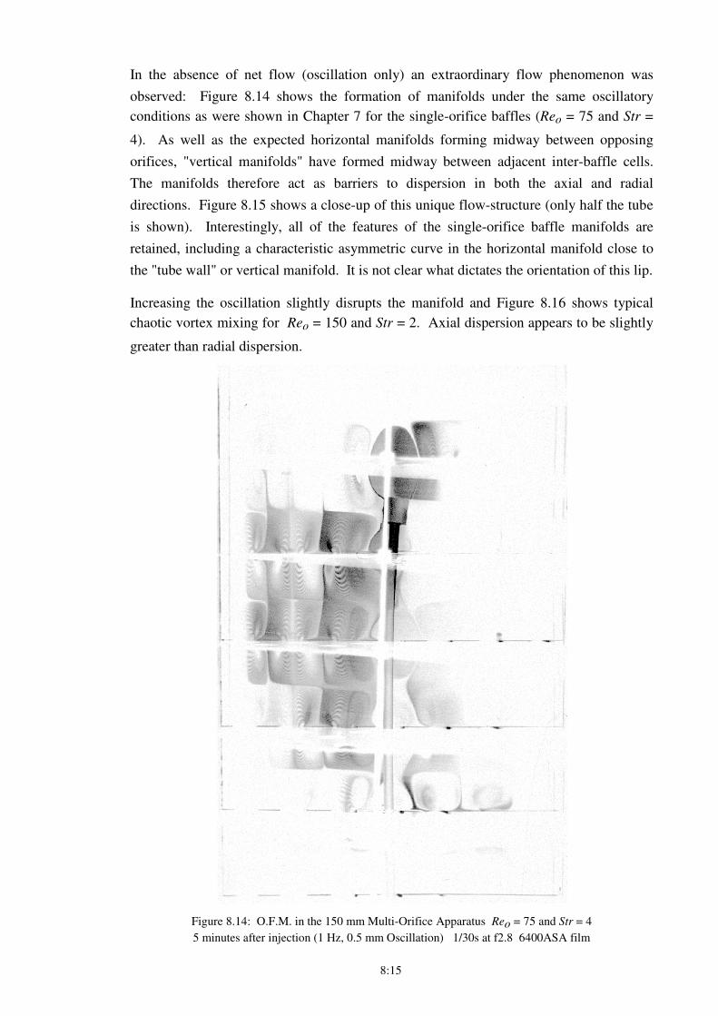
8:15
In the absence of net flow (oscillation only) an extraordinary flow phenomenon was
observed: Figure 8.14 shows the formation of manifolds under the same oscillatory
conditions as were shown in Chapter 7 for the single-orifice baffles (Reo = 75 and Str =
4). As well as the expected horizontal manifolds forming midway between opposing
orifices, "vertical manifolds" have formed midway between adjacent inter-baffle cells.
The manifolds therefore act as barriers to dispersion in both the axial and radial
directions. Figure 8.15 shows a close-up of this unique flow-structure (only half the tube
is shown). Interestingly, all of the features of the single-orifice baffle manifolds are
retained, including a characteristic asymmetric curve in the horizontal manifold close to
the "tube wall" or vertical manifold. It is not clear what dictates the orientation of this lip.
Increasing the oscillation slightly disrupts the manifold and Figure 8.16 shows typical
chaotic vortex mixing for Reo = 150 and Str = 2. Axial dispersion appears to be slightly
greater than radial dispersion.
Figure 8.14: O.F.M. in the 150 mm Multi-Orifice Apparatus Reo = 75 and Str = 4
5 minutes after injection (1 Hz, 0.5 mm Oscillation) 1/30s at f2.8 6400ASA film
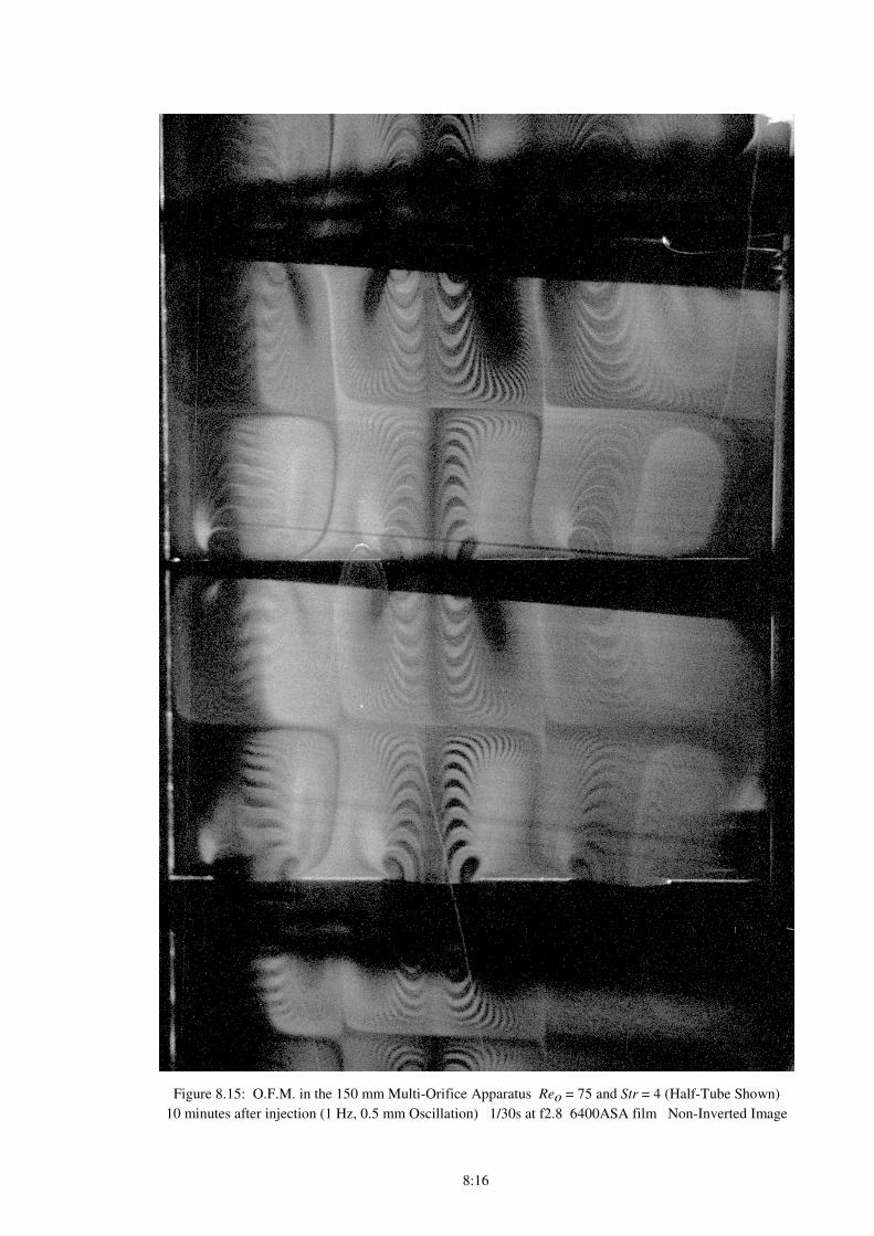
8:16
Figure 8.15: O.F.M. in the 150 mm Multi-Orifice Apparatus Reo = 75 and Str = 4 (Half-Tube Shown)
10 minutes after injection (1 Hz, 0.5 mm Oscillation) 1/30s at f2.8 6400ASA film Non-Inverted Image
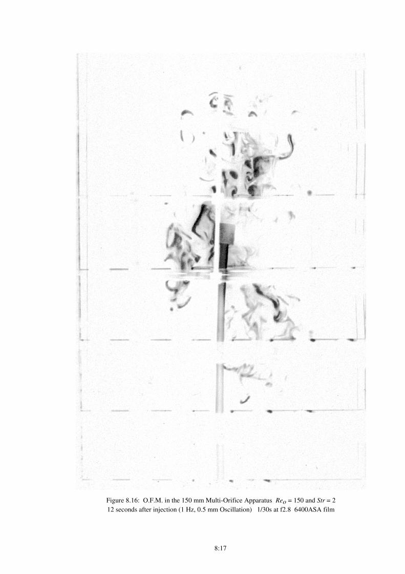
8:17
Figure 8.16: O.F.M. in the 150 mm Multi-Orifice Apparatus Reo = 150 and Str = 2
12 seconds after injection (1 Hz, 0.5 mm Oscillation) 1/30s at f2.8 6400ASA film
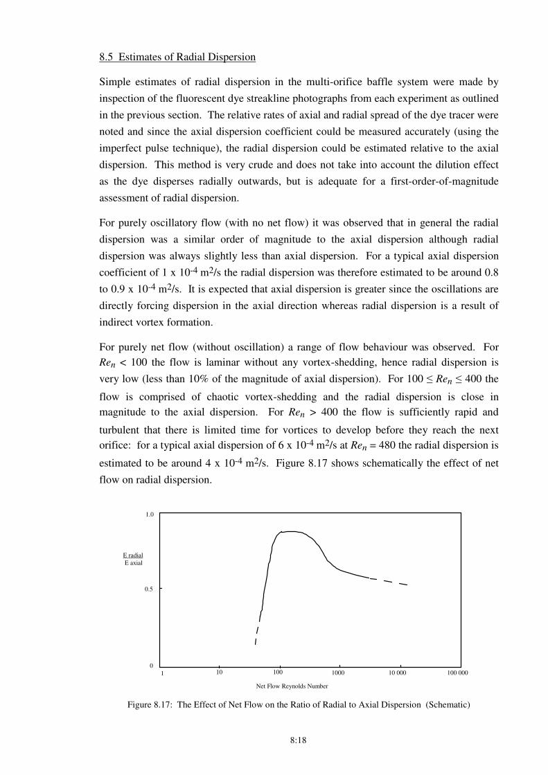
8:18
8.5 Estimates of Radial Dispersion
Simple estimates of radial dispersion in the multi-orifice baffle system were made by
inspection of the fluorescent dye streakline photographs from each experiment as outlined
in the previous section. The relative rates of axial and radial spread of the dye tracer were
noted and since the axial dispersion coefficient could be measured accurately (using the
imperfect pulse technique), the radial dispersion could be estimated relative to the axial
dispersion. This method is very crude and does not take into account the dilution effect
as the dye disperses radially outwards, but is adequate for a first-order-of-magnitude
assessment of radial dispersion.
For purely oscillatory flow (with no net flow) it was observed that in general the radial
dispersion was a similar order of magnitude to the axial dispersion although radial
dispersion was always slightly less than axial dispersion. For a typical axial dispersion
coefficient of 1 x 10⁻⁴ m2/s the radial dispersion was therefore estimated to be around 0.8
to 0.9 x 10⁻⁴ m2/s. It is expected that axial dispersion is greater since the oscillations are
directly forcing dispersion in the axial direction whereas radial dispersion is a result of
indirect vortex formation.
For purely net flow (without oscillation) a range of flow behaviour was observed. For
Ren < 100 the flow is laminar without any vortex-shedding, hence radial dispersion is
very low (less than 10% of the magnitude of axial dispersion). For 100 ≤ Ren ≤ 400 the
flow is comprised of chaotic vortex-shedding and the radial dispersion is close in
magnitude to the axial dispersion. For Ren > 400 the flow is sufficiently rapid and
turbulent that there is limited time for vortices to develop before they reach the next
orifice: for a typical axial dispersion of 6 x 10⁻⁴ m2/s at Ren = 480 the radial dispersion is
estimated to be around 4 x 10⁻⁴ m2/s. Figure 8.17 shows schematically the effect of net
flow on radial dispersion.
E radial
E axial
1.0
0.5
0
Net Flow Reynolds Number
1 10 100 1000 10 000 100 000
Figure 8.17: The Effect of Net Flow on the Ratio of Radial to Axial Dispersion (Schematic)
8:19
For net flow and oscillations together in the multi-orifice system, the flow can be
categorised into two distinct regimes: firstly for Ren > 100 and / or Reo > 100 the flow is
chaotic and the radial dispersion is of order 80% of the magnitude of the axial dispersion;
secondly for Ren < 100 and Reo < 100 a range of radial dispersion is seen depending upon
the precise relative values of Ren, Reo and Str. For this second regime radial dispersion is
always less than axial dispersion and as a rule-of-thumb if Ren and Reo are of similar
magnitude then increasing the Strouhal number decreases radial dispersion (because
smaller amplitude oscillations are less effective at creating large vortices).
SUMMARY:
This chapter has presented a preliminary investigation into the use of multi-orifice baffles
as a method of scaling-up O.F.M.. The multi-orifice design appears particularly attractive
because of the potential ease of manufacture for large plant but also because of the
similarity of the observed fluid mechanics and axial dispersion between single and multi-
orifice baffle designs. This means that in principle laboratory scale experiments could be
carried out and the results be used with reasonable confidence to predict axial dispersion
(and mixing intensity) in a very much larger industrial scale multi-orifice baffle reactor.
9:1
9. Discussion
The work presented in this thesis has extended the range and understanding of axial
dispersion measurements and fluid mechanics in O.F.M. and has addressed the issue of
scale-up. This chapter aims to discuss the work in the wider context of the existing
literature and of industrial application. A number of different areas will be addressed.
§9.1 discusses measured axial dispersion in O.F.M. and its relationship to the observed
fluid mechanics. §9.2 compares flow visualisations and the measured values of axial
dispersion with the results available in the literature. §9.3 examines the potential
applicability of either single-orifice or multi-orifice baffles for industrial scale processes.
§9.4 and §9.5 address the issues of heat transfer and energy dissipation in large-scale
O.F.M.. §9.6 addresses possible engineering considerations for the construction of
industrial scale O.F.M..
9.1 Relating Axial Dispersion Measurements to Flow Visualisations
Flow visualisations and axial dispersion measurements have been made across a wide
range of conditions for oscillatory flow mixing in baffled tubes (Chapters 5, 6 and 7).
Experimental and simulated results have been produced in both cases. The cases of net
flow only, oscillations only, and net flow with oscillations have been investigated: the
observed flow has ranged from creeping laminar flow to fully turbulent flow and
measured axial dispersion has ranged from the order of 10-7 to 10-1 m2/s. This section
summarises those results and their interrelationship.
NET FLOW ONLY OR OSCILLATIONS ONLY
It appears from experimental flow visualisations that with either oscillations only
(without a net flow) or net flow only (without oscillations) the flow is axisymmetric and
laminar at low Reynolds number flows, but that at Reynolds numbers of order 80 and
above the flow becomes asymmetric (Chapter 7) for the geometry investigated. With
increasing Reynolds number the flow becomes increasingly chaotic (with the formation of
large-scale vortices by the flow past the baffles) until for Reynolds numbers of
approximately 800 and above the flow appears to be fully turbulent. The flow is assumed
to be fully turbulent when individual vortices are no longer clearly visible in the flow and
the fluorescent dye tracer disperses rapidly and homogeneously (i.e. discrete streaklines
are not visible in the flow). These flow regimes for either net flow or oscillatory flow
alone are summarised in Figure 9.1. The indicated values of axial dispersion are
approximate and vary depending upon whether net flow or oscillation is involved and
also the Strouhal number of the oscillation.
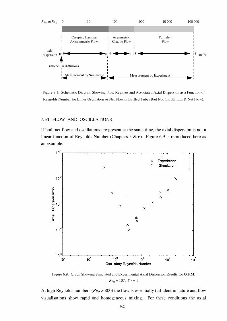
9:2
0 10 100 1000 10 000 100 000Reo or Ren
Creeping Laminar
Axisymmetric Flow
Asymmetric
Chaotic Flow
Turbulent
Flow
10-9 10-4 10-3 10-1
(molecular diffusion)
axial
dispersion m2/s
Measurement by Simulation Measurement by Experiment
Figure 9.1: Schematic Diagram Showing Flow Regimes and Associated Axial Dispersion as a Function of
Reynolds Number for Either Oscillation or Net Flow in Baffled Tubes (but Not Oscillations & Net Flow).
NET FLOW AND OSCILLATIONS
If both net flow and oscillations are present at the same time, the axial dispersion is not a
linear function of Reynolds Number (Chapters 5 & 6). Figure 6.9 is reproduced here as
an example.
Figure 6.9: Graph Showing Simulated and Experimental Axial Dispersion Results for O.F.M.
Ren = 107, Str = 1
At high Reynolds numbers (Reo > 800) the flow is essentially turbulent in nature and flow
visualisations show rapid and homogeneous mixing. For these conditions the axial
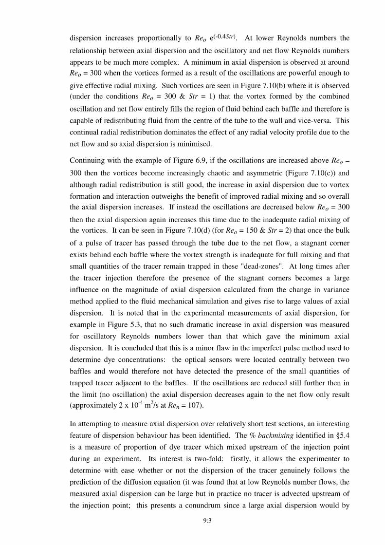
9:3
dispersion increases proportionally to Reo e(-0.4Str). At lower Reynolds numbers the
relationship between axial dispersion and the oscillatory and net flow Reynolds numbers
appears to be much more complex. A minimum in axial dispersion is observed at around
Reo = 300 when the vortices formed as a result of the oscillations are powerful enough to
give effective radial mixing. Such vortices are seen in Figure 7.10(b) where it is observed
(under the conditions Reo = 300 & Str = 1) that the vortex formed by the combined
oscillation and net flow entirely fills the region of fluid behind each baffle and therefore is
capable of redistributing fluid from the centre of the tube to the wall and vice-versa. This
continual radial redistribution dominates the effect of any radial velocity profile due to the
net flow and so axial dispersion is minimised.
Continuing with the example of Figure 6.9, if the oscillations are increased above Reo =
300 then the vortices become increasingly chaotic and asymmetric (Figure 7.10(c)) and
although radial redistribution is still good, the increase in axial dispersion due to vortex
formation and interaction outweighs the benefit of improved radial mixing and so overall
the axial dispersion increases. If instead the oscillations are decreased below Reo = 300
then the axial dispersion again increases this time due to the inadequate radial mixing of
the vortices. It can be seen in Figure 7.10(d) (for Reo = 150 & Str = 2) that once the bulk
of a pulse of tracer has passed through the tube due to the net flow, a stagnant corner
exists behind each baffle where the vortex strength is inadequate for full mixing and that
small quantities of the tracer remain trapped in these "dead-zones". At long times after
the tracer injection therefore the presence of the stagnant corners becomes a large
influence on the magnitude of axial dispersion calculated from the change in variance
method applied to the fluid mechanical simulation and gives rise to large values of axial
dispersion. It is noted that in the experimental measurements of axial dispersion, for
example in Figure 5.3, that no such dramatic increase in axial dispersion was measured
for oscillatory Reynolds numbers lower than that which gave the minimum axial
dispersion. It is concluded that this is a minor flaw in the imperfect pulse method used to
determine dye concentrations: the optical sensors were located centrally between two
baffles and would therefore not have detected the presence of the small quantities of
trapped tracer adjacent to the baffles. If the oscillations are reduced still further then in
the limit (no oscillation) the axial dispersion decreases again to the net flow only result
(approximately 2 x 10⁻⁴
m2/s at Ren = 107).
In attempting to measure axial dispersion over relatively short test sections, an interesting
feature of dispersion behaviour has been identified. The % backmixing identified in §5.4
is a measure of proportion of dye tracer which mixed upstream of the injection point
during an experiment. Its interest is two-fold: firstly, it allows the experimenter to
determine with ease whether or not the dispersion of the tracer genuinely follows the
prediction of the diffusion equation (it was found that at low Reynolds number flows, the
measured axial dispersion can be large but in practice no tracer is advected upstream of
the injection point; this presents a conundrum since a large axial dispersion would by
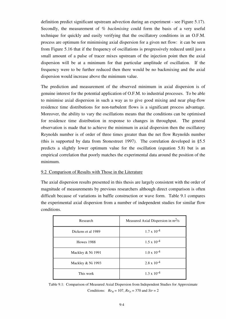
9:4
definition predict significant upstream advection during an experiment - see Figure 5.17).
Secondly, the measurement of % backmixing could form the basis of a very useful
technique for quickly and easily verifying that the oscillatory conditions in an O.F.M.
process are optimum for minimising axial dispersion for a given net flow: it can be seen
from Figure 5.16 that if the frequency of oscillations is progressively reduced until just a
small amount of a pulse of tracer mixes upstream of the injection point then the axial
dispersion will be at a minimum for that particular amplitude of oscillation. If the
frequency were to be further reduced then there would be no backmixing and the axial
dispersion would increase above the minimum value.
The prediction and measurement of the observed minimum in axial dispersion is of
genuine interest for the potential application of O.F.M. to industrial processes. To be able
to minimise axial dispersion in such a way as to give good mixing and near plug-flow
residence time distributions for non-turbulent flows is a significant process advantage.
Moreover, the ability to vary the oscillations means that the conditions can be optimised
for residence time distribution in response to changes in throughput. The general
observation is made that to achieve the minimum in axial dispersion then the oscillatory
Reynolds number is of order of three times greater than the net flow Reynolds number
(this is supported by data from Stonestreet 1997). The correlation developed in §5.5
predicts a slightly lower optimum value for the oscillation (equation 5.8) but is an
empirical correlation that poorly matches the experimental data around the position of the
minimum.
9.2 Comparison of Results with Those in the Literature
The axial dispersion results presented in this thesis are largely consistent with the order of
magnitude of measurements by previous researchers although direct comparison is often
difficult because of variations in baffle construction or wave form. Table 9.1 compares
the experimental axial dispersion from a number of independent studies for similar flow
conditions.
Research Measured Axial Dispersion in m2/s
Dickens et al 1989 1.7 x 10⁻⁴
Howes 1988 1.5 x 10⁻⁴
Mackley & Ni 1991 1.0 x 10⁻⁴
Mackley & Ni 1993 2.8 x 10⁻⁴
This work 1.3 x 10⁻⁴
Table 9.1: Comparison of Measured Axial Dispersion from Independent Studies for Approximate
Conditions: Ren = 107, Reo = 370 and Str = 2
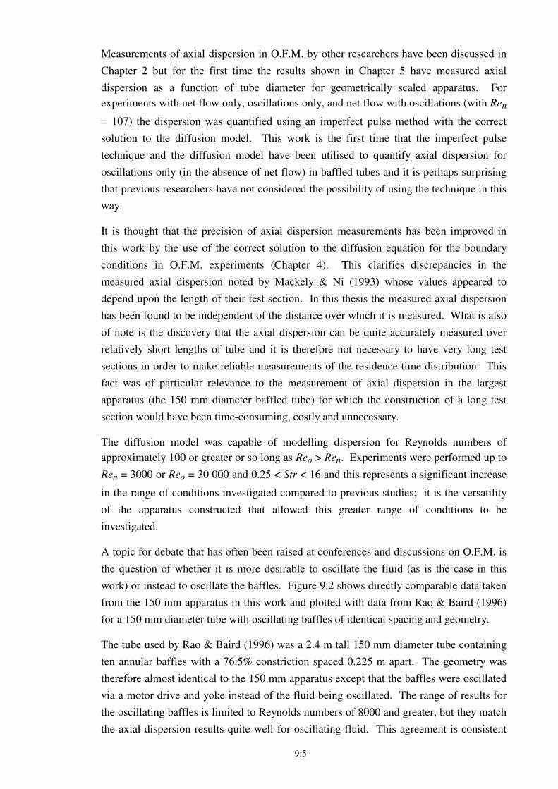
9:5
Measurements of axial dispersion in O.F.M. by other researchers have been discussed in
Chapter 2 but for the first time the results shown in Chapter 5 have measured axial
dispersion as a function of tube diameter for geometrically scaled apparatus. For
experiments with net flow only, oscillations only, and net flow with oscillations (with Ren
= 107) the dispersion was quantified using an imperfect pulse method with the correct
solution to the diffusion model. This work is the first time that the imperfect pulse
technique and the diffusion model have been utilised to quantify axial dispersion for
oscillations only (in the absence of net flow) in baffled tubes and it is perhaps surprising
that previous researchers have not considered the possibility of using the technique in this
way.
It is thought that the precision of axial dispersion measurements has been improved in
this work by the use of the correct solution to the diffusion equation for the boundary
conditions in O.F.M. experiments (Chapter 4). This clarifies discrepancies in the
measured axial dispersion noted by Mackely & Ni (1993) whose values appeared to
depend upon the length of their test section. In this thesis the measured axial dispersion
has been found to be independent of the distance over which it is measured. What is also
of note is the discovery that the axial dispersion can be quite accurately measured over
relatively short lengths of tube and it is therefore not necessary to have very long test
sections in order to make reliable measurements of the residence time distribution. This
fact was of particular relevance to the measurement of axial dispersion in the largest
apparatus (the 150 mm diameter baffled tube) for which the construction of a long test
section would have been time-consuming, costly and unnecessary.
The diffusion model was capable of modelling dispersion for Reynolds numbers of
approximately 100 or greater or so long as Reo > Ren. Experiments were performed up to
Ren = 3000 or Reo = 30 000 and 0.25 < Str < 16 and this represents a significant increase
in the range of conditions investigated compared to previous studies; it is the versatility
of the apparatus constructed that allowed this greater range of conditions to be
investigated.
A topic for debate that has often been raised at conferences and discussions on O.F.M. is
the question of whether it is more desirable to oscillate the fluid (as is the case in this
work) or instead to oscillate the baffles. Figure 9.2 shows directly comparable data taken
from the 150 mm apparatus in this work and plotted with data from Rao & Baird (1996)
for a 150 mm diameter tube with oscillating baffles of identical spacing and geometry.
The tube used by Rao & Baird (1996) was a 2.4 m tall 150 mm diameter tube containing
ten annular baffles with a 76.5% constriction spaced 0.225 m apart. The geometry was
therefore almost identical to the 150 mm apparatus except that the baffles were oscillated
via a motor drive and yoke instead of the fluid being oscillated. The range of results for
the oscillating baffles is limited to Reynolds numbers of 8000 and greater, but they match
the axial dispersion results quite well for oscillating fluid. This agreement is consistent
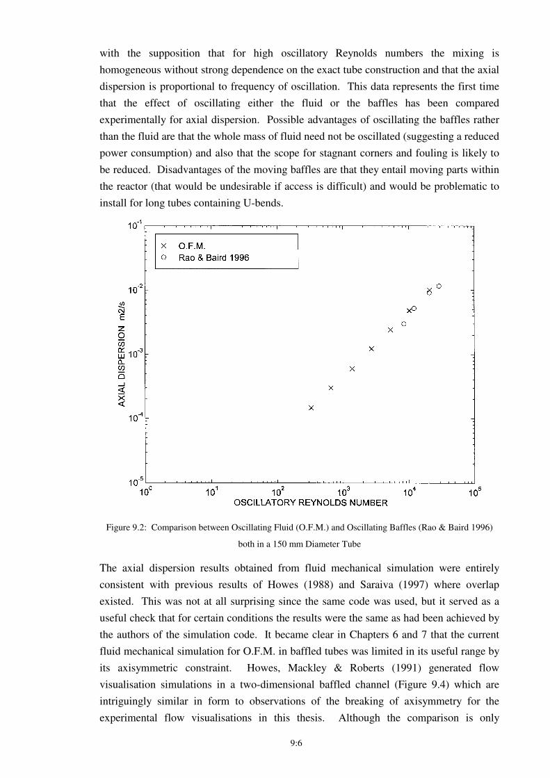
9:6
with the supposition that for high oscillatory Reynolds numbers the mixing is
homogeneous without strong dependence on the exact tube construction and that the axial
dispersion is proportional to frequency of oscillation. This data represents the first time
that the effect of oscillating either the fluid or the baffles has been compared
experimentally for axial dispersion. Possible advantages of oscillating the baffles rather
than the fluid are that the whole mass of fluid need not be oscillated (suggesting a reduced
power consumption) and also that the scope for stagnant corners and fouling is likely to
be reduced. Disadvantages of the moving baffles are that they entail moving parts within
the reactor (that would be undesirable if access is difficult) and would be problematic to
install for long tubes containing U-bends.
Figure 9.2: Comparison between Oscillating Fluid (O.F.M.) and Oscillating Baffles (Rao & Baird 1996)
both in a 150 mm Diameter Tube
The axial dispersion results obtained from fluid mechanical simulation were entirely
consistent with previous results of Howes (1988) and Saraiva (1997) where overlap
existed. This was not at all surprising since the same code was used, but it served as a
useful check that for certain conditions the results were the same as had been achieved by
the authors of the simulation code. It became clear in Chapters 6 and 7 that the current
fluid mechanical simulation for O.F.M. in baffled tubes was limited in its useful range by
its axisymmetric constraint. Howes, Mackley & Roberts (1991) generated flow
visualisation simulations in a two-dimensional baffled channel (Figure 9.4) which are
intriguingly similar in form to observations of the breaking of axisymmetry for the
experimental flow visualisations in this thesis. Although the comparison is only
9:7
qualitative, it suggests that the development of a fluid mechanical code which would
allow asymmetric flow in baffled tubes would be of considerable interest as a means of
further investigating O.F.M..
(a) Reo = 100, Str = 1 (Axisymmetric Flow)
(b) Reo = 300, Str = 1 (Showing Breaking of Symmetry)
Figure 9.4: Numerical Simulations by Howes et al (1991) for a Baffled Channel during One Oscillation
(reproduced with permission)
9.3 Multi-Orifice Baffles as a Route to Scale-Up
The findings in Chapter 8 have established that the use of multi-orifice baffles is of
considerable interest as a means to scaling-up O.F.M.. The case study example given in
§8.1 has been modified for the case of multi-orifice baffles and is shown in Figure 9.5.
The multi-orifice baffles appear quite similar in configuration to those typically found in
reciprocating plate columns (§2.3.2). This is a useful comparison since it has already
been established that for turbulent flows, axial dispersion is the same in O.F.M. as for
reciprocating annular baffles (Figure 9.3) of similar geometry. It is therefore not
unreasonable to suppose that the results of research on reciprocating plate columns with
similar geometry to multi-orifice O.F.M. can be of relevance to O.F.M. for turbulent
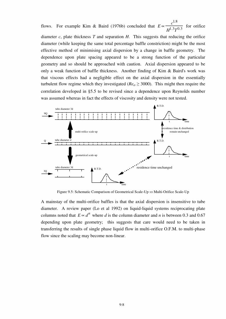
9:8
flows. For example Kim & Baird (1976b) concluded that E ∝c1.8
H1.3T0.3 for orifice
diameter c, plate thickness T and separation H. This suggests that reducing the orifice
diameter (while keeping the same total percentage baffle constriction) might be the most
effective method of minimising axial dispersion by a change in baffle geometry. The
dependence upon plate spacing appeared to be a strong function of the particular
geometry and so should be approached with caution. Axial dispersion appeared to be
only a weak function of baffle thickness. Another finding of Kim & Baird's work was
that viscous effects had a negligible effect on the axial dispersion in the essentially
turbulent flow regime which they investigated (Reo ≥ 3000). This might then require the
correlation developed in §5.5 to be revised since a dependence upon Reynolds number
was assumed whereas in fact the effects of viscosity and density were not tested.
Figure 9.5: Schematic Comparison of Geometrical Scale-Up vs Multi-Orifice Scale-Up
A mainstay of the multi-orifice baffles is that the axial dispersion is insensitive to tube
diameter. A review paper (Lo et al 1992) on liquid-liquid systems reciprocating plate
columns noted that E ∝ dn
where d is the column diameter and n is between 0.3 and 0.67
depending upon plate geometry; this suggests that care would need to be taken in
transferring the results of single phase liquid flow in multi-orifice O.F.M. to multi-phase
flow since the scaling may become non-linear.
time
R.T.D.tube diameter d
tube diameter 3d
geometrical scale-up t
time
R.T.D.
t
residence time & distribution
remain unchanged
Q
3Q
time
R.T.D.
t
tube diameter 3d
multi-orifice scale-up
residence time & distribution
remain unchanged
9Q
residence time unchanged
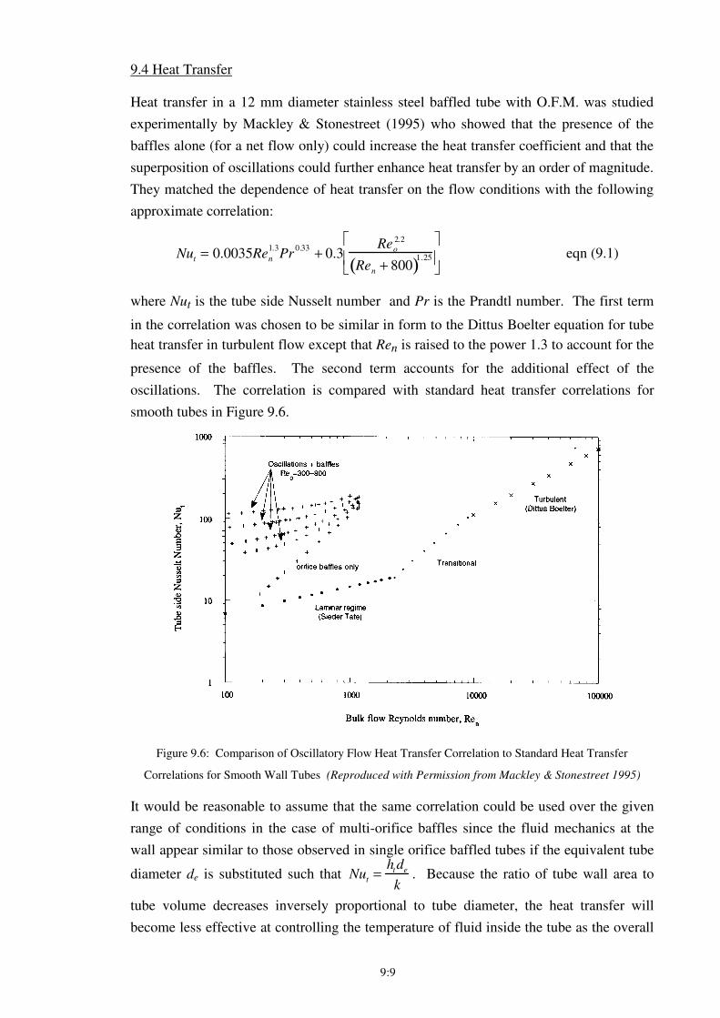
9:9
9.4 Heat Transfer
Heat transfer in a 12 mm diameter stainless steel baffled tube with O.F.M. was studied
experimentally by Mackley & Stonestreet (1995) who showed that the presence of the
baffles alone (for a net flow only) could increase the heat transfer coefficient and that the
superposition of oscillations could further enhance heat transfer by an order of magnitude.
They matched the dependence of heat transfer on the flow conditions with the following
approximate correlation:
Nut = 0.0035Ren
1.3Pr
0.33+ 0.3
Reo
2.2
Ren + 800( )1.25
eqn (9.1)
where Nut is the tube side Nusselt number and Pr is the Prandtl number. The first term
in the correlation was chosen to be similar in form to the Dittus Boelter equation for tube
heat transfer in turbulent flow except that Ren is raised to the power 1.3 to account for the
presence of the baffles. The second term accounts for the additional effect of the
oscillations. The correlation is compared with standard heat transfer correlations for
smooth tubes in Figure 9.6.
Figure 9.6: Comparison of Oscillatory Flow Heat Transfer Correlation to Standard Heat Transfer
Correlations for Smooth Wall Tubes (Reproduced with Permission from Mackley & Stonestreet 1995)
It would be reasonable to assume that the same correlation could be used over the given
range of conditions in the case of multi-orifice baffles since the fluid mechanics at the
wall appear similar to those observed in single orifice baffled tubes if the equivalent tube
diameter de is substituted such that Nut =htde
k. Because the ratio of tube wall area to
tube volume decreases inversely proportional to tube diameter, the heat transfer will
become less effective at controlling the temperature of fluid inside the tube as the overall
9:10
tube diameter increases. For processes where temperature control is critical the
maximum tube diameter that can be used for multi-orifice baffles may be limited by the
decreasing tube wall area per unit volume of fluid in the tube.
In the case of geometrical scale-up (without the use of multi-orifice baffles) the tube side
heat transfer coefficient reduces inversely proportional to tube diameter (under similar
dynamic conditions i.e. for a constant Nusselt number). For low Reynolds numbers it is
speculated that buoyancy would have an increasingly important effect on the fluid
mechanics the larger the diameter of the tube and would eventually dominate the forced
oscillations. An indication of this was seen experimentally when taking video pictures of
low Reynolds number flows in the 24 mm apparatus using a powerful floodlight: strong
convective flow was observed due to heating of the tube wall on the side of the tube
nearest the floodlight which caused the flow to become asymmetric.
9.5 Energy Dissipation
Baird & Stonestreet (1995) examined the energy dissipation associated with O.F.M. using
the same experimental apparatus as Mackley & Stonestreet (1995). By considering the
combination of the inertial and frictional pressure drops in O.F.M. they developed a
correlation (equation 9.2) for power density εv that gave good agreement with
experimental measurements of power density:
Correlation for Power Density:
εv
=1.5ρω3 xo
2l
HS (W/m3) eqn (9.2)
(after Baird & Stonestreet (1995))
where H is the spacing between baffles, S the fractional open area of baffle and l a
characteristic mixing length. Their correlation was based upon an eddy enhancement
model for the frictional pressure drop and the only adjustable parameter was the mixing
length l . They determined the best fit value of l to be 7 mm i.e. of similar magnitude to
the orifice diameter in their experiments (although they acknowledged that changing
either the baffle geometry or spacing could affect l). Power densities in the range 100 to
10 000 W/m3 were observed for O.F.M. with 220 ≤ Reo ≤ 6750 and 0.15 ≤ Str ≤ 0.95.
The mixing length l could be expected to remain the same for multi-orifice baffles of
similar equivalent diameter (since the scale of the fluid mechanics is similar) but for
geometrically scaled baffled tubes it is not known how l would vary with tube diameter:
for a given Reo and Str the inertial contribution to equation 9.2 would be expected to
remain constant per unit volume but the frictional contribution would probably decrease
with increasing tube diameter.
It is recognised that these calculations of power density do not include the additional
energy dissipated in the mechanical oscillator due to piston inertia and friction as well as
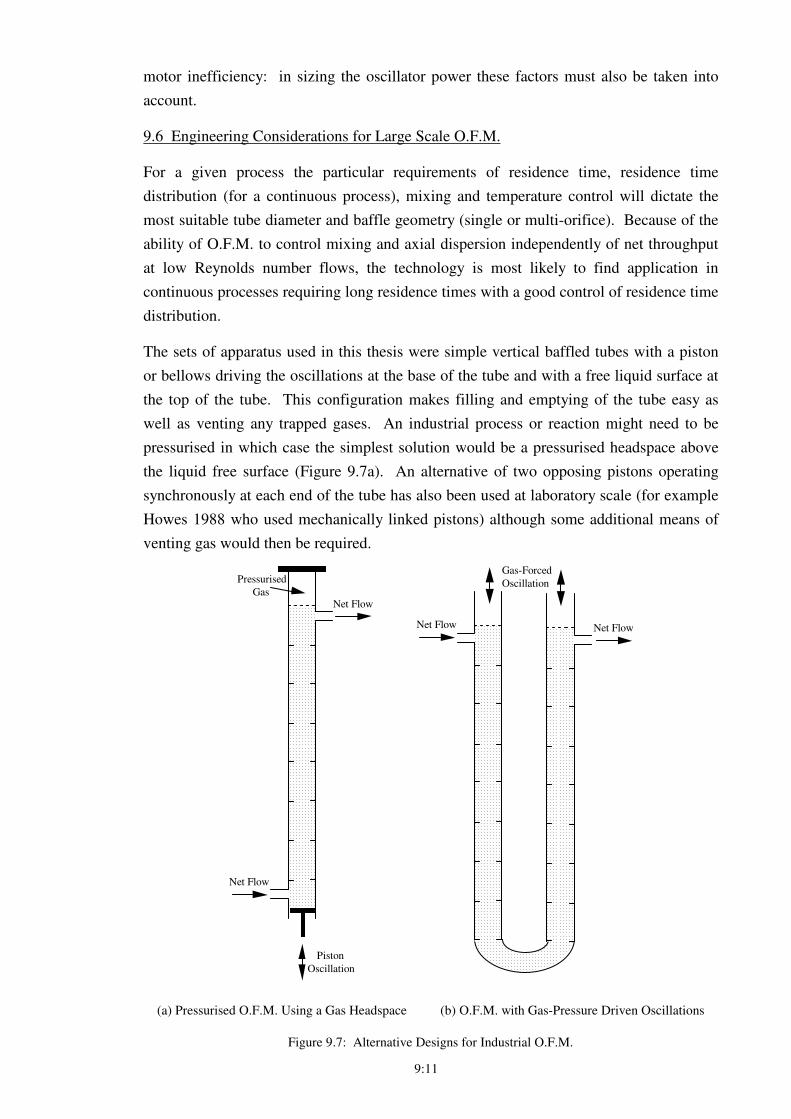
9:11
motor inefficiency: in sizing the oscillator power these factors must also be taken into
account.
9.6 Engineering Considerations for Large Scale O.F.M.
For a given process the particular requirements of residence time, residence time
distribution (for a continuous process), mixing and temperature control will dictate the
most suitable tube diameter and baffle geometry (single or multi-orifice). Because of the
ability of O.F.M. to control mixing and axial dispersion independently of net throughput
at low Reynolds number flows, the technology is most likely to find application in
continuous processes requiring long residence times with a good control of residence time
distribution.
The sets of apparatus used in this thesis were simple vertical baffled tubes with a piston
or bellows driving the oscillations at the base of the tube and with a free liquid surface at
the top of the tube. This configuration makes filling and emptying of the tube easy as
well as venting any trapped gases. An industrial process or reaction might need to be
pressurised in which case the simplest solution would be a pressurised headspace above
the liquid free surface (Figure 9.7a). An alternative of two opposing pistons operating
synchronously at each end of the tube has also been used at laboratory scale (for example
Howes 1988 who used mechanically linked pistons) although some additional means of
venting gas would then be required.
Piston
Oscillation
Net Flow
Net Flow
Pressurised
Gas
Net Flow Net Flow
Gas-Forced
Oscillation
(a) Pressurised O.F.M. Using a Gas Headspace (b) O.F.M. with Gas-Pressure Driven Oscillations
Figure 9.7: Alternative Designs for Industrial O.F.M.
9:12
An alternative design option would be to use manometer-style oscillating columns (as
used by the nuclear reprocessing industry for liquid-liquid contacting) where the
oscillations are driven by gas pressure difference at the top of a U-tube (Figure 9.7b).
This design would be suited to low frequency oscillations (Hill et al), but unsuitable if
rapid oscillations were required since the forces required to accelerate and decelerate the
fluid would be difficult to achieve with gas pressure alone. In the latter case a rigid piston
and cylinder oscillator would be preferable.
The use of piston and cylinder arrangements to transmit the oscillations is quite effective
and uses standard "off-the-shelf" sealing technology that under normal operating
conditions will last many oscillatory cycles, although there is always the potential for
leakage if the seals are damaged or worn. The piston seals used in the 150 mm apparatus
oscillator remained in good condition after approximately 500 000 cycles without any
appreciable leakage. The stainless steel bellows used for the 24 mm apparatus were also
successful and did not leak (lasting approximately 1 500 000 cycles without failure),
although it is thought that larger scale bellows would be prone to distortion under load
and are not generally designed to withstand rapid oscillations without the risk of fatigue.
The use of servo-hydraulics to power oscillations in O.F.M. has been shown to be a
versatile method. It has several advantages including "off-the-shelf" components that are
cheap and easy to replace, flexible control of frequency and amplitude of oscillation,
physical compactness, and spark-free operation in a hazardous area.
A potential issue for O.F.M. in very long tubes with large frictional and inertial pressure
drops is the possibility of cavitation. This might be avoided by overall pressurisation of
the tube, or alternatively the tube would need to be designed in several sections separated
by flow pumps.
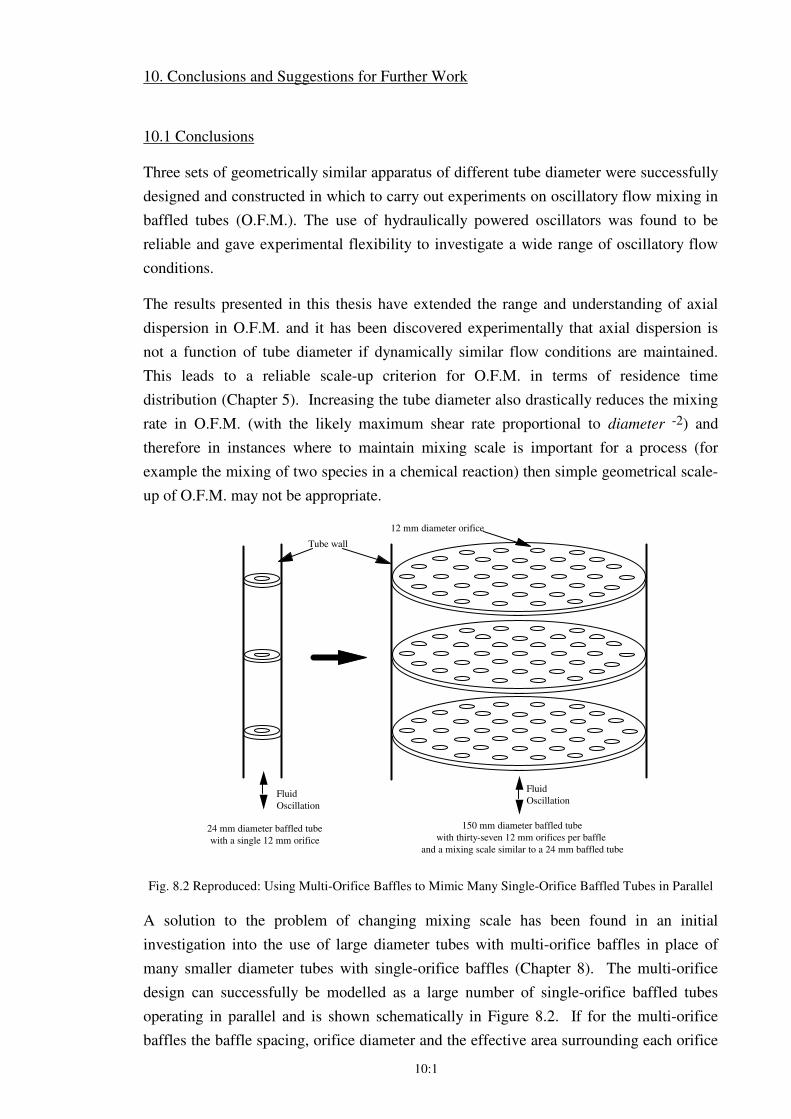
10:1
10. Conclusions and Suggestions for Further Work
10.1 Conclusions
Three sets of geometrically similar apparatus of different tube diameter were successfully
designed and constructed in which to carry out experiments on oscillatory flow mixing in
baffled tubes (O.F.M.). The use of hydraulically powered oscillators was found to be
reliable and gave experimental flexibility to investigate a wide range of oscillatory flow
conditions.
The results presented in this thesis have extended the range and understanding of axial
dispersion in O.F.M. and it has been discovered experimentally that axial dispersion is
not a function of tube diameter if dynamically similar flow conditions are maintained.
This leads to a reliable scale-up criterion for O.F.M. in terms of residence time
distribution (Chapter 5). Increasing the tube diameter also drastically reduces the mixing
rate in O.F.M. (with the likely maximum shear rate proportional to diameter -2) and
therefore in instances where to maintain mixing scale is important for a process (for
example the mixing of two species in a chemical reaction) then simple geometrical scale-
up of O.F.M. may not be appropriate.
Fluid
Oscillation
24 mm diameter baffled tube
with a single 12 mm orifice
150 mm diameter baffled tube
with thirty-seven 12 mm orifices per baffle
and a mixing scale similar to a 24 mm baffled tube
Fluid
Oscillation
Tube wall
12 mm diameter orifice
Fig. 8.2 Reproduced: Using Multi-Orifice Baffles to Mimic Many Single-Orifice Baffled Tubes in Parallel
A solution to the problem of changing mixing scale has been found in an initial
investigation into the use of large diameter tubes with multi-orifice baffles in place of
many smaller diameter tubes with single-orifice baffles (Chapter 8). The multi-orifice
design can successfully be modelled as a large number of single-orifice baffled tubes
operating in parallel and is shown schematically in Figure 8.2. If for the multi-orifice
baffles the baffle spacing, orifice diameter and the effective area surrounding each orifice
10:2
is equivalent to the single-orifice baffles then the fluid mechanics, measured axial
dispersion and mixing scale are similarly comparable. This means that experiments can
be carried out at laboratory scale with O.F.M. in single-orifice baffled tubes and the
results can be scaled-up with confidence by large orders of magnitude to a multi-orifice
design. (The scale-up factor achieved in this work was an increase in volumetric flowrate
of 39 times for the same dynamic conditions. It is speculated that very much larger
increases could be achieved without affecting the fluid mechanics, axial dispersion or
mixing scale using larger diameter baffles with a commensurately greater number of
orifices).
Axial dispersion has been quantified for a wide range of dynamic conditions in O.F.M.
using the imperfect pulse technique and the diffusion model. The literature relating to
solving the diffusion equation (equation 2.14) has been clarified in Chapter 4 and a
reliable method for quantifying axial dispersion measured over short tube lengths in
O.F.M. has been developed. The method is quite general and could be applied to any
situation involving axial dispersion in a long tube.
A useful fluorescent dye streakline flow visualisation method has been developed and
successfully applied to O.F.M. (Chapter 7). The technique has advantages over previous
flow visualisation methods applied to O.F.M. and it allows direct comparisons to be made
between flow in tubes of different diameter. The technique has been used to show that
the fluid mechanics of O.F.M. are not strongly affected by tube diameter. Specific flow
regimes ranging from creeping laminar to chaotic and fully turbulent have been identified
and used to explain trends in the measured axial dispersion.
An unusual flow phenomenon has been identified for the geometry studied in the absence
of net flow and at low oscillatory Reynolds numbers: vortices moving in opposing
directions meet midway between two baffles and create strong radial flow from the centre
of the tube to the wall and act as barriers to dispersion. These fluid "manifolds" (Chapter
7) are an interesting and unique flow structure: well mixed regions of fluid are separated
by the manifolds across which the only mechanism for axial dispersion is molecular
diffusion. The manifold flow structure observed in multi-orifice baffles (Figures 8.14 &
8.15) is even more striking in that axial, toroidal and radially oriented manifolds can all
exist simultaneously, creating a three-dimensional structure of compartmentalised mixing
regions with minimal exchange of fluid into neighbouring compartments. If a batch
process required gentle localised stretch-fold mixing with minimal bulk mixing then
manifolds would be highly desirable.
The results of both axial dispersion measurements and flow visualisations have been
simulated using a computerised fluid mechanical simulation. The simulation was
constrained to predict axisymmetric flow and was therefore limited to flows with a
Reynolds number of less than approximately 100. Since most experimental results were
restricted to Reynolds numbers of greater than 100 by the limitations of the diffusion
10:3
model, the fluid mechanical simulation is a useful tool for extending the range of dynamic
conditions which can be investigated for axisymmetric flows. Although the fluid
mechanical simulation only provided a small overlap with experimental results the
observed fluid mechanics and axial dispersion matched well for experiment and
simulation, giving confidence in the validity of both techniques.
The experimental results for axial dispersion have been correlated as a function of Ren,
Reo and Str (Chapter 5, §5.5). This empirical correlation is most successful at high
Reynolds numbers (> 800). At intermediate oscillatory Reynolds numbers (30 < Reo <
800) the correlation shows some deviations from the experimental data when a small net
flow is introduced although the correct order of magnitude for axial dispersion is
predicted. The overall best-fit correlation is only dependent upon Ren0.8 and Reoe(-0.4Str)
for a water-based system:
E = 7.0 × 10⁻⁷
Ren
0.8+ 7.5× 10
−7Reo e
−0.4Str( )+
3.0 × 10⁻¹²Ren
1.6
7.0 × 10⁻⁷
Ren
0.8+ 7.5× 10
−7Reo e
−0.4Str( )
(m2/s) eqn (5.6) reproduced
It is concluded that O.F.M. is a technology which in general lends itself readily to scaling-
up from laboratory to pilot plant scale, and most probably to industrial scale.
Experiments performed on small laboratory apparatus (containing less than one litre of
fluid) can with confidence be used to predict mixing behaviour in much larger plant
(containing hundreds of litres of fluid.)
10.2 Suggestions for Further Work
A wide-ranging study of axial dispersion in O.F.M. has been presented using results from
both experiment and simulation. The limitations of the work are recognised in that the
upper limit for simulation results is a Reynolds number of order 100 (above which the
simulation cannot predict the flow which becomes asymmetric) while the lower extent of
experimental results is also at a similar order of magnitude Reynolds number (below
which the diffusion model is unsuccessful at quantifying axial dispersion over short
distances). There is therefore a very limited overlap between the two sets of results (from
experiment and from simulation). It is suggested that a useful course of work for the
future would be to aim to extend the valid range of results for the simulation and / or the
experimental model. In the case of the simulation, the code would have to be adapted to
include non-axisymmetric flows which might extend the validity of the simulation up to
Reynolds numbers of order 800. Turbulent flow modelling would be required to further
extend the range of the simulation to higher Reynolds numbers. In the case of the
experimental technique for determining axial dispersion, an alternative to the diffusion
model would have to be sought in order to extend the useful range of the imperfect pulse
technique.
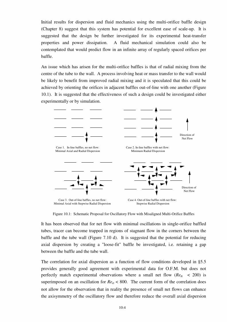
10:4
Initial results for dispersion and fluid mechanics using the multi-orifice baffle design
(Chapter 8) suggest that this system has potential for excellent ease of scale-up. It is
suggested that the design be further investigated for its experimental heat-transfer
properties and power dissipation. A fluid mechanical simulation could also be
contemplated that would predict flow in an infinite array of regularly spaced orifices per
baffle.
An issue which has arisen for the multi-orifice baffles is that of radial mixing from the
centre of the tube to the wall. A process involving heat or mass transfer to the wall would
be likely to benefit from improved radial mixing and it is speculated that this could be
achieved by orienting the orifices in adjacent baffles out-of-line with one another (Figure
10.1). It is suggested that the effectiveness of such a design could be investigated either
experimentally or by simulation.
Case 1. In-line baffles, no net flow:
Minimal Axial and Radial Dispersion
Case 2. In-line baffles with net flow:
Minimum Radial Dispersion
Direction of
Net Flow
Case 3. Out-of-line baffles, no net flow:
Minimal Axial with Stepwise Radial Dispersion
Case 4. Out-of-line baffles with net flow:
Stepwise Radial Dispersion
Direction of
Net Flow
Figure 10.1: Schematic Proposal for Oscillatory Flow with Misaligned Multi-Orifice Baffles
It has been observed that for net flow with minimal oscillations in single-orifice baffled
tubes, tracer can become trapped in regions of stagnant flow in the corners between the
baffle and the tube wall (Figure 7.10 d). It is suggested that the potential for reducing
axial dispersion by creating a "loose-fit" baffle be investigated, i.e. retaining a gap
between the baffle and the tube wall.
The correlation for axial dispersion as a function of flow conditions developed in §5.5
provides generally good agreement with experimental data for O.F.M. but does not
perfectly match experimental observations where a small net flow (Ren < 200) is
superimposed on an oscillation for Reo < 800. The current form of the correlation does
not allow for the observation that in reality the presence of small net flows can enhance
the axisymmetry of the oscillatory flow and therefore reduce the overall axial dispersion

10:5
rather than increase it as might have been intuitively expected. It is therefore suggested
that an alternative form of correlation be considered which could reflect this behaviour.
References: 1
References
Aris R. 1956 "On the dispersion of a solute in a fluid flowing through a tube" Proc. Roy.
Soc. Lond. A235 pp 67-77
Aris R. 1959(a) "Notes on the diffusion-type model for longitudinal mixing in flow"
Chem. Eng. Sci. Vol 9 pp 266-267
Aris R. 1959(b) "The longitudinal diffusion coefficient in flow through a tube with
stagnant pockets" Chem. Eng. Sci. Vol 11 pp 194-198
Aris R. 1960 "On the dispersion of a solute in pulsating flow through a tube" Proc. Roy.
Soc. Lond. A259 pp 370-376
Baird M.H.I. 1966 "Vibrations and pulsation" British Chem. Eng. Vol 11 No 1 pp 20-25
Baird M.H.I. 1974 "Axial dispersion in a pulsed plate column" Can. J. Chem. Eng. Vol
52 pp 750-757
Baird M.H.I. & Stonestreet P. 1995 "Energy dissipation in oscillatory flow within a
baffled tube" Trans IChemE Vol 73 Part A pp 503-511
Baird M.H.I. & Rama Rao N.V. 1996 “Hydrodynamics of reciprocating plate columns”
2nd
Conference on Pulsatile Flow, June 3rd
, University of Strathclyde, Scotland
Bischoff K.B. 1960 "Notes on the diffusion-type model for longitudinal mixing in flow"
Chem. Eng. Sci. Vol 12 pp 69-70
Brunold C.R., Hunns J.C.B., Mackley M.R. & Thompson J.W. 1989 "Experimental
observations on flow patterns and energy losses for oscillatory flow in ducts
containing sharp edges" Chem. Eng. Sci. Vol 44 No 5 pp 1227-1244
Carberry J.J. & Bretton R.H. 1958 "Axial dispersion of mass in flow through fixed beds"
A.I.Ch.E. Journal Vol 4 No 3 pp 367-375
Crittenden B.D., Field R.W. & Pervez M.I. 1995 "Oscillatory flow in packed beds and
baffled tubes. A unifiying approach to the interpretation of experimental data" Chem.
Eng. Sci. Vol 50 No 23 pp 3839-3845
Danckwerts P.V. 1953 "Continuous flow systems" Chem. Eng. Sci. Vol 2 No 1 pp 1-13
References: 2
Dickens A.W., Mackley M.R. & Williams H.R. 1989 "Experimental residence time
distribution measurements for unsteady flow in baffled tubes" Chem. Eng. Sci. Vol 44
No 7 pp 1471-1479
Gilibaro L.G. 1978 “On the residence time distribution for systems with open boundaries”
Chem. Eng. Sci. Vol 33 pp 487-492
Goebel J.C., Booij K. & Fortuin J.M.H. 1986 "Axial dispersion in single-phase flow in
pulsed packed columns" Chem. Eng. Sci. Vol 41 No 12 pp 3197-3203
Hayden E.S.S. 1997 "A Quantitative Study of Oscillatory Flows in Plain and Baffled
Tubes" Thesis, University of Cambridge
Hewgill M.R., Mackley M.R., Pandit A.B. & Pannu S.S. 1993 "Enhancement of gas-
liquid mass transfer using oscillatory flow in a baffled tube" Chem. Eng. Sci. Vol 48
No 4 pp 799-809
Hill H.J., R and DD, BNF Plc Sellafield “Analysis and design of pulsing systems for air
pulsed solvent extraction columns” IChemE Symposium Series no 103 pp 87-101
Howes T. 1988 "On the dispersion of unsteady flow in baffled tubes" PhD Thesis,
University of Cambridge
Howes T. & Mackley M.R. 1990 "Experimental axial dispersion for oscillatory flow
through a baffled tube" Chem. Eng. Sci. Vol 45 No 5 pp 1349-1358
Howes T., Mackley M.R. & Roberts E.P.L. 1991 "The simulation of chaotic mixing and
dispersion for periodic flows in baffled channels” Chem. Eng. Sci. Vol 46 No 7 pp
1669-1677
Hwu T., Sobey I.J. & Bellhouse B.J. 1996 "Observation of concentration dispersion in
unsteady deflected flows” Chem. Eng. Sci. Vol 51 pp 3373-3390
Keulegan G.H. & Carpenter L.H. 1958 "Forces on cylinders and plates in an oscillatory
fluid" Journal of Research (National Bureau of Standards) Vol 60 pp 423-440
Kim S.D. & Baird M.H.I. 1976(a) "Axial dispersion in a reciprocating plate extraction
column" Can. J. Chem. Eng. Vol 54 pp 81-89
References: 3
Kim S.D. & Baird M.H.I. 1976(b) "Effect of hole size on hydrodynamics of a
reciprocating perforated plate extraction column" Can. J. Chem. Eng. Vol 54 pp 235-
237
Knott G.F. & Mackley M.R. 1980 "On eddy motions near platees and ducts induced by
water waves and periodic flows" Proc. Roy. Soc. Lond. A294 pp 599-623
Levenspiel O. & Smith W.K. 1957 "Notes on the diffusion type model for the
longitudinal mixing of fluids in flow" Chem. Eng. Sci. Vol 6 pp 227-233
Levenspiel O. 1972 "Chemical Reaction Engineering" John Wiley & Sons 2nd Ed. N.Y.
Lo T.C., Baird M.H.I. & Rama Rao N.V. 1992 "The reciprocating plate column -
development and applications" Chem. Eng Comm. Vol 116 pp 67-88
Long J.T. 1967 "Engineering for nuclear fuel reprocessing" Gordon & Breach Science
Publishers Inc. N.Y.
Lounes M & Thibault J. 1996 “Axial Dispersion in a Reciprocating Plate Column” Can.
J. Chem. Eng. Vol 74 pp 187-194
Mackay M.E., Mackley M.R. & Wang Y. 1991 "Oscillatory flow within tubes containing
wall or central baffles" Trans IChemE Vol 69 Part A pp 506-513
Mackley M.R. 1987 "Using oscillatory flow to improve performace" Chemical Engineer,
February Edition pp 18-20
Mackley M.R., Tweddle G.M. & Wyatt I.D. 1990 "Experimental heat transfer
measurements for pulsatile flow in baffled tubes" Chem. Eng. Sci. Vol 45 No 5 pp
1237-1242
Mackley M.R. 1991 "Process innovation using oscillatory flow within baffled tubes"
Trans IChemE Vol 69 pp 197-199
Mackley M.R. & Ni X. 1991 "Mixing and dispersion in a baffled tube for steady laminar
and pulsatile flow" Chem. Eng. Sci. Vol 46 No 12 pp 3139-3151
Mackley M.R. & Roberts E.P.L. 1991 "Mixing and flow patterns for unsteady flow in
baffled channels" American Soc. Mech. Engineers FED Vol 127 pp57-64
References: 4
Mackley M.R., Smith K.B. & Wise N.P. 1993 "The mixing and separation of particle
suspensions using oscillatory flow in baffled tubes" Trans IChemE Vol 71 Part A pp
649-656
Mackley M.R. & Ni X. 1993 "Experimental fluid dispersion measurements in periodic
baffled tube arrays" Chem. Eng. Sci. Vol 48 No 18 pp 3293-3305
Mackley M.R. & Roberts E.P.L. 1995 "The simulation of stretch rates for the quantitative
prediction and mapping of mixing within a channel flow" Chem. Eng. Sci. Vol 50 No
23 pp 3727-3746
Mackley M.R. & Stonestreet P. 1995 "Heat transfer and associated energy dissipation for
oscillatory flow in baffled tubes" Chem. Eng. Sci. Vol 50 No 14 pp 2211-2224
Mackley M.R., Stonestreet P., Thurston N.C. & Wiseman J.S. 1998 "Evaluation of a
Novel Self-Aerating, Oscillating Baffle Column" Can. J. Chem. Eng. Vol 76 pp 5-10
Mak A.N.S., Koning C.A.J., Hamersma P.J. & Fortuin J.M.H. 1991 "Axial dispersion in
single-phase flow in a pulsed packed column containing structured packing" Chem.
Eng. Sci. Vol 46 No 3 pp 819-826
Mecklenburg J.C. & Hartland S. 1975 "The theory of backmixing" John Wiley & Sons
London
Nauman E.B. & Mallikarjun R. 1983 "Generalized boundary conditions for the axial
dispersion model" Chem. Engineering Journal Vol 26 pp 231-237
Ni X. & Mackley M.R. 1993 "Chemical Reaction in Batch Pulsatile Flow and Stirred
Tank Reactors" Chem. Engineering Journal Vol 52 pp 107-114
Ni X. 1994 "Residence time distribution measurements in a pulsed baffled tube bundle" J.
Chem Tech. Biotechnol. Vol 59 pp 213-221
Ni X. 1995 "A study of fluid dispersion on oscillatory flow through a baffled tube" J.
Chem Tech. Biotechnol. Vol 64 pp 165-174
Ni X., Gao S., Cumming R.H. & Pritchard D.W. 1995 "A Comparative Study of Mass
Transfer in Yeast for a Batch Pulsed Baffled Bioreactor and a Stirred Tank
Fermenter" Chem. Eng. Sci. Vol 50 No 13 pp 2127-2136
References: 5
Ni X. & Gao S. 1996 "Mass transfer characteristics of a pilot pulsed baffled reactor" J.
Chem Tech. Biotechnol. Vol 65 pp 65-71
Ni X. & Gough P. 1997 "On the discussion of the dimensionless groups governing
oscillatory flow in a baffles tube" Chem. Eng. Sci. Vol 52 No 18 pp 3209-3212
Ni X., Brogan G., Struthers A., Bennett D.C. and Wilson S.F. 1998 "A systematic study
of the effect of geometrical parameters on mixing time in oscillatory baffles columns"
Trans IChemE Vol 76 Part A pp 635-642
Perry 1984 “Chemical Engineer’s Handbook” 6th
Ed. McGraw-Hill
Reeder M., Janz E. and Myers K. 1997 "Experimental Investigation of Viscosity Ratio
Effects on the Performance of Static Mixers" AIChemE Annual Meeting, Los Angeles
Saraiva, R.M.D.C.N. 1997 "The Characterisation of Mixing for Oscillatory Flow within
Baffled Tubes" PhD Thesis, University of Cambridge
Scott D.M. 1997 (private communication)
Simons A.J.F., van Sluys R., Goebel J.C. & Fortuin J.M.H. 1986 "Axial dispersion in
pulsed packed columns on both laboratory and industrial scale" Proceedings of
I.S.E.C. Muenchen
Sobey I.J. 1985 "Dispersion caused by separation during oscillatory flow through a
furrowed channel" Chem. Eng. Sci. Vol 40 No 11 pp 2129-2134
Stevens G.W. & Baird M.H.I. 1990 "A model for axial mixing in reciprocating plate
columns" Chem. Eng. Sci. Vol 46 No 2 pp 457-465
Stonestreet P. 1997 (private communication)
Taylor G.I. 1953 "Dispersion of soluble matter in solvent flowing slowly through a tube"
Proc. Roy. Soc. Lond. A219 pp 186-203
Taylor G.I. 1954 "The dispersion of matter in turbulent flow through a pipe" Proc. Roy.
Soc. Lond. A223 pp 446-467
van der Laan 1958 "Notes on the diffusion-type model for the longitudinal mixing in
flow" Chem. Eng. Sci. Vol 7 pp 187-191
References: 6
Wang Y., Howell J.A., Field R.W. & Mackley M.R. 1994 "Oscillatory flow within
porous tubes containing wall or central baffles" Trans IChemE Vol 72 Part A pp 686-
693
Westerterp K.R., van Swaaij W.P.M. & Beenackers A.A.C.M. 1984 "Chemical Reactor
Design and Operation" John Wiley & Sons London
Williams D.H. & Fleming I. 1989 "Spectroscopic methods in organic chemistry"
McGraw-Hill 4th Ed London
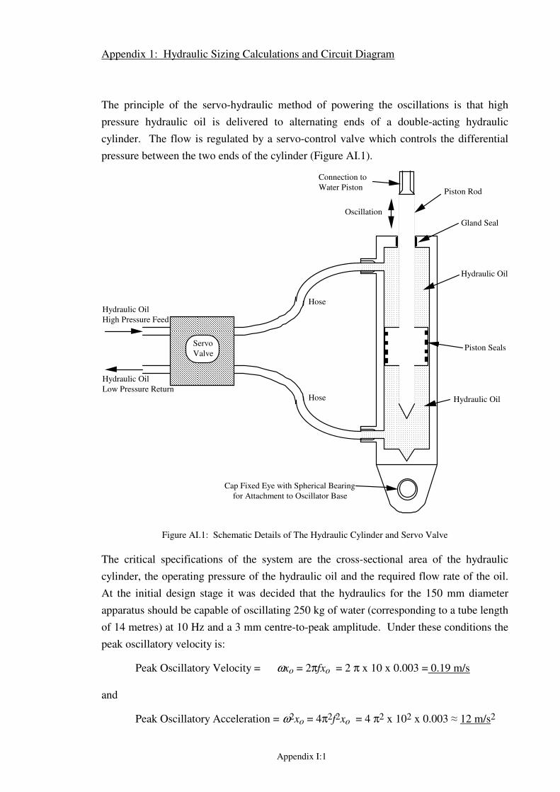
Appendix I:1
Appendix 1: Hydraulic Sizing Calculations and Circuit Diagram
The principle of the servo-hydraulic method of powering the oscillations is that high
pressure hydraulic oil is delivered to alternating ends of a double-acting hydraulic
cylinder. The flow is regulated by a servo-control valve which controls the differential
pressure between the two ends of the cylinder (Figure AI.1).
Hydraulic Oil
Hydraulic Oil
Piston Seals
Gland Seal
Piston Rod
Hydraulic Oil
High Pressure Feed
Hydraulic Oil
Low Pressure Return
Servo
Valve
Hose
Hose
Oscillation
Connection to
Water Piston
Cap Fixed Eye with Spherical Bearing
for Attachment to Oscillator Base
Figure AI.1: Schematic Details of The Hydraulic Cylinder and Servo Valve
The critical specifications of the system are the cross-sectional area of the hydraulic
cylinder, the operating pressure of the hydraulic oil and the required flow rate of the oil.
At the initial design stage it was decided that the hydraulics for the 150 mm diameter
apparatus should be capable of oscillating 250 kg of water (corresponding to a tube length
of 14 metres) at 10 Hz and a 3 mm centre-to-peak amplitude. Under these conditions the
peak oscillatory velocity is:
Peak Oscillatory Velocity = ωxo = 2πfxo = 2 π x 10 x 0.003 = 0.19 m/s
and
Peak Oscillatory Acceleration = ω2xo = 4π2f2xo = 4 π2 x 102 x 0.003 ≈ 12 m/s2
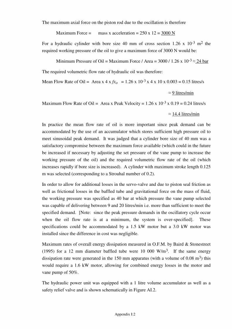
Appendix I:2
The maximum axial force on the piston rod due to the oscillation is therefore
Maximum Force = mass x acceleration = 250 x 12 = 3000 N
For a hydraulic cylinder with bore size 40 mm of cross section 1.26 x 10⁻³ m2 the
required working pressure of the oil to give a maximum force of 3000 N would be:
Minimum Pressure of Oil = Maximum Force / Area = 3000 / 1.26 x 10⁻³ ≈ 24 bar
The required volumetric flow rate of hydraulic oil was therefore:
Mean Flow Rate of Oil = Area x 4 x fxo = 1.26 x 10-3 x 4 x 10 x 0.003 = 0.15 litres/s
≈ 9 litres/min
Maximum Flow Rate of Oil = Area x Peak Velocity = 1.26 x 10-3 x 0.19 = 0.24 litres/s
≈ 14.4 litres/min
In practice the mean flow rate of oil is more important since peak demand can be
accommodated by the use of an accumulator which stores sufficient high pressure oil to
meet sinusoidal peak demand. It was judged that a cylinder bore size of 40 mm was a
satisfactory compromise between the maximum force available (which could in the future
be increased if necessary by adjusting the set pressure of the vane pump to increase the
working pressure of the oil) and the required volumetric flow rate of the oil (which
increases rapidly if bore size is increased). A cylinder with maximum stroke length 0.125
m was selected (corresponding to a Strouhal number of 0.2).
In order to allow for additional losses in the servo-valve and due to piston seal friction as
well as frictional losses in the baffled tube and gravitational force on the mass of fluid,
the working pressure was specified as 40 bar at which pressure the vane pump selected
was capable of delivering between 9 and 20 litres/min i.e. more than sufficient to meet the
specified demand. [Note: since the peak pressure demands in the oscillatory cycle occur
when the oil flow rate is at a minimum, the system is over-specified]. These
specifications could be accommodated by a 1.5 kW motor but a 3.0 kW motor was
installed since the difference in cost was negligible.
Maximum rates of overall energy dissipation measured in O.F.M. by Baird & Stonestreet
(1995) for a 12 mm diameter baffled tube were 10 000 W/m3. If the same energy
dissipation rate were generated in the 150 mm apparatus (with a volume of 0.08 m3) this
would require a 1.6 kW motor, allowing for combined energy losses in the motor and
vane pump of 50%.
The hydraulic power unit was equipped with a 1 litre volume accumulator as well as a
safety relief valve and is shown schematically in Figure AI.2.
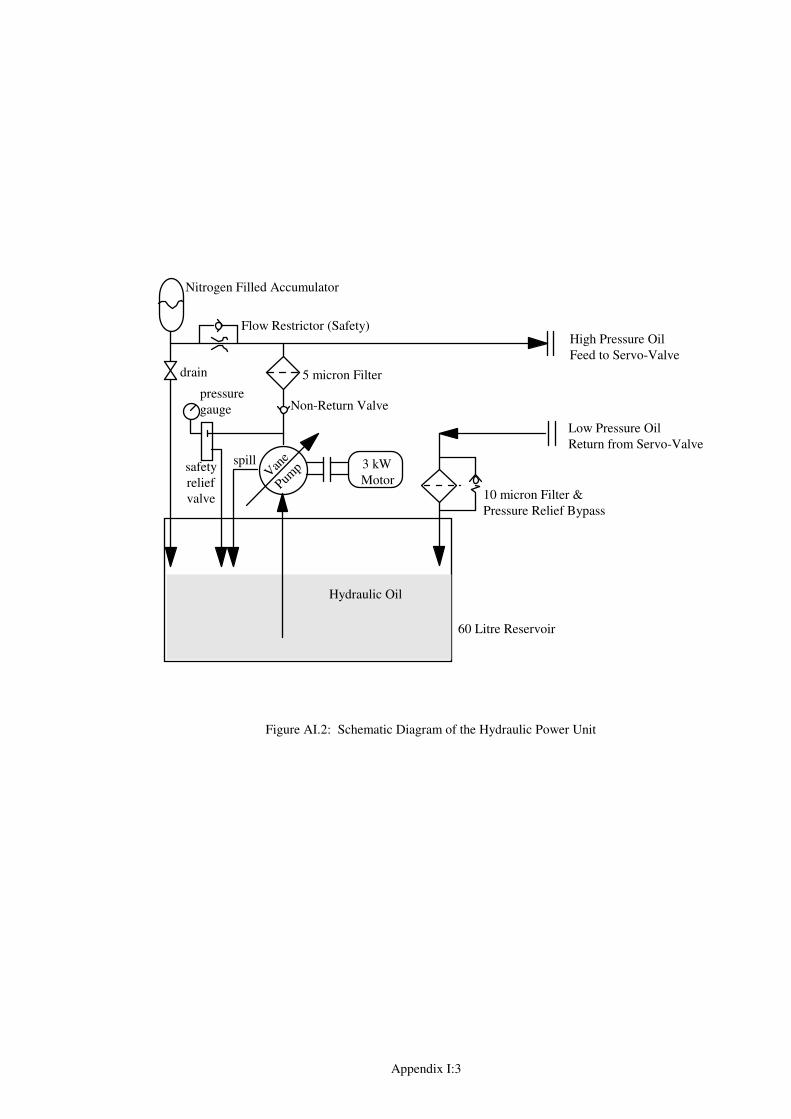
Appendix I:3
3 kW
MotorV
ane
Pump
spill
High Pressure Oil
Feed to Servo-Valve
Low Pressure Oil
Return from Servo-Valve
Nitrogen Filled Accumulator
Flow Restrictor (Safety)
10 micron Filter &
Pressure Relief Bypass
5 micron Filter
Non-Return Valve
60 Litre Reservoir
Hydraulic Oil
drain
pressure
gauge
safety
relief
valve
Figure AI.2: Schematic Diagram of the Hydraulic Power Unit
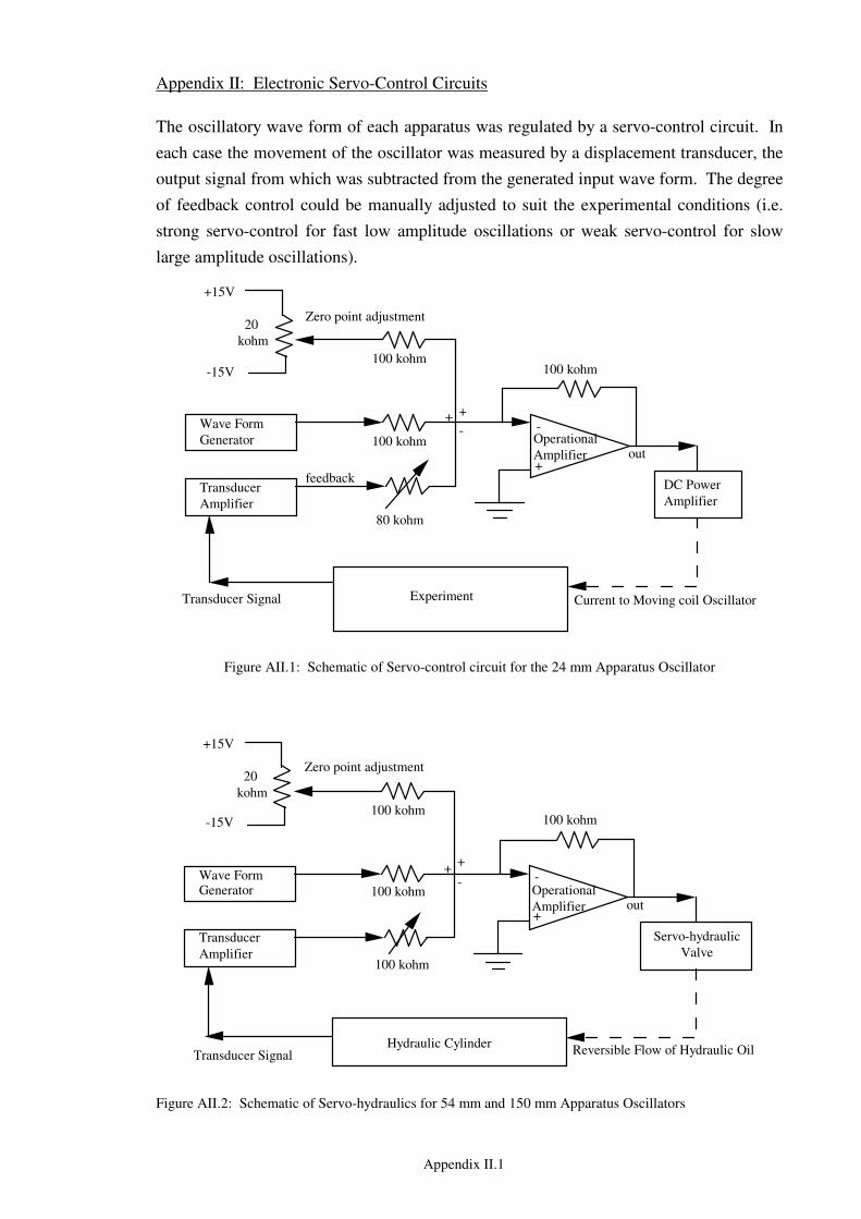
Appendix II.1
Appendix II: Electronic Servo-Control Circuits
The oscillatory wave form of each apparatus was regulated by a servo-control circuit. In
each case the movement of the oscillator was measured by a displacement transducer, the
output signal from which was subtracted from the generated input wave form. The degree
of feedback control could be manually adjusted to suit the experimental conditions (i.e.
strong servo-control for fast low amplitude oscillations or weak servo-control for slow
large amplitude oscillations).
Operational
Amplifier
Wave Form
Generator
Transducer
Amplifier
100 kohm
80 kohm
DC Power
Amplifier
Transducer Signal Current to Moving coil OscillatorExperiment
-
+
100 kohm
+15V
-15V100 kohm
20
kohm
Zero point adjustment
out
feedback
-
++
Figure AII.1: Schematic of Servo-control circuit for the 24 mm Apparatus Oscillator
Operational
Amplifier
Wave Form Generator
Transducer
Amplifier
100 kohm
100 kohm
Servo-hydraulic
Valve
Transducer Signal Reversible Flow of Hydraulic OilHydraulic Cylinder
-
+
100 kohm
+15V
-15V100 kohm
20
kohm
Zero point adjustment
out
-
++
Figure AII.2: Schematic of Servo-hydraulics for 54 mm and 150 mm Apparatus Oscillators
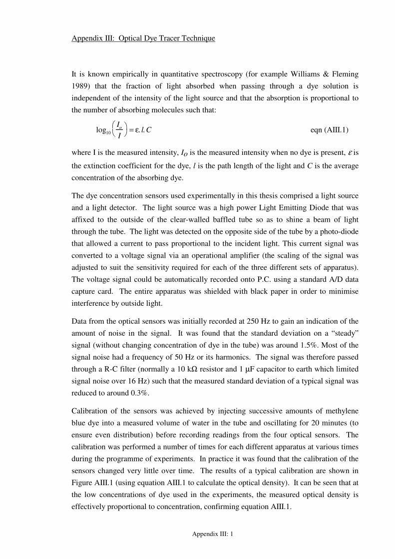
Appendix III: 1
Appendix III: Optical Dye Tracer Technique
It is known empirically in quantitative spectroscopy (for example Williams & Fleming
1989) that the fraction of light absorbed when passing through a dye solution is
independent of the intensity of the light source and that the absorption is proportional to
the number of absorbing molecules such that:
log10
Io
I
= ε. l.C eqn (AIII.1)
where I is the measured intensity, Io is the measured intensity when no dye is present, ε is
the extinction coefficient for the dye, l is the path length of the light and C is the average
concentration of the absorbing dye.
The dye concentration sensors used experimentally in this thesis comprised a light source
and a light detector. The light source was a high power Light Emitting Diode that was
affixed to the outside of the clear-walled baffled tube so as to shine a beam of light
through the tube. The light was detected on the opposite side of the tube by a photo-diode
that allowed a current to pass proportional to the incident light. This current signal was
converted to a voltage signal via an operational amplifier (the scaling of the signal was
adjusted to suit the sensitivity required for each of the three different sets of apparatus).
The voltage signal could be automatically recorded onto P.C. using a standard A/D data
capture card. The entire apparatus was shielded with black paper in order to minimise
interference by outside light.
Data from the optical sensors was initially recorded at 250 Hz to gain an indication of the
amount of noise in the signal. It was found that the standard deviation on a “steady”
signal (without changing concentration of dye in the tube) was around 1.5%. Most of the
signal noise had a frequency of 50 Hz or its harmonics. The signal was therefore passed
through a R-C filter (normally a 10 kΩ resistor and 1 µF capacitor to earth which limited
signal noise over 16 Hz) such that the measured standard deviation of a typical signal was
reduced to around 0.3%.
Calibration of the sensors was achieved by injecting successive amounts of methylene
blue dye into a measured volume of water in the tube and oscillating for 20 minutes (to
ensure even distribution) before recording readings from the four optical sensors. The
calibration was performed a number of times for each different apparatus at various times
during the programme of experiments. In practice it was found that the calibration of the
sensors changed very little over time. The results of a typical calibration are shown in
Figure AIII.1 (using equation AIII.1 to calculate the optical density). It can be seen that at
the low concentrations of dye used in the experiments, the measured optical density is
effectively proportional to concentration, confirming equation AIII.1.
Appendix III: 2
The lines are of different gradient: this may be explained by there being different path
lengths for each optical sensor depending upon the precise alignment of the L.E.D. and
the exact position of the sensor. The gradients were automatically determined in a
specially-written Matlab analysis programme that generated a data file containing the
measured value of ε.l for sensor 1 together with a correction factor for sensors 2, 3 and 4
which could be used in the subsequent data analysis (see Appendix IV) to eliminate
differences between the sensors. The correction factors were close to unity, typically in
the range 0.95 to 1.05.
sensor 1
sensor 2
sensor 3
sensor 4
Figure AIII.1: Calibration of Four Experimental Optical Sensors in the 24 mm Apparatus
Appendix IV: 1
Appendix 4: Matlab Analysis Programme for Axial Dispersion
The programme net7 is used to analyse axial dispersion from experiments with net flow;
after initially clearing the memory it calls a series of subroutines. Variations on net7 are
given for the cases of no net flow and for net flow without oscillation.
Note that % at any point in a line allows annotations to be written in the programme.
% ********************************************************************
% net7 - Programme to read in and process axial dispersion data
% ********************************************************************
clear %remove all pre-existing variables from the workspace
variab7a %read in all the fixed variables (tube diameter, net flow, sampling rate, raw data file name, storage file name etc.)
rdin7 %read in raw data from 12-bit binary file and arrange as a 16-bit matrix
start7 %detect the start-point of the experiment (the moment of dye injection)
baselin7 %measure the baseline readings for the 4 optical sensors with no dye present
trimdat7 %top-and-tail the data matrix so that it starts at the moment of dye injection
timaxis7 %deduce the timebase of the data matrix from the sampling frequency
wave7 %determine the oscillation frequency and amplitude, and detect irregularities
reduce7 %reduce the size of the data matrix by averaging over each oscillation
od_conc7 %compute the optical density (hence concentration) for each optical sensor
area7 %calculate the area under each sensor's concentration-time profile
normalz7 %normalise each sensor's concentration-time profile
graphff %plot the concentration-time profiles for all 4 optical sensors
moment1 %calculate the first moment of area of each concentration-time profile
moment2 %calculate the second moment of area of each concentration-time profile
optim123 %determine the value of the axial dispersion coefficient E which causes the model predicted concentration-time profile to most closely match the experimental concentration-time profile for each pair of downstream sensors (1 to 2, 2 to 3, 1 to 3)
Hz_ctpa_Reo_Ren=[cyclefrequency ctpamplitude*1000 reynoldsosc reynoldsnet] %display the cycle frequency in Hz, the centre-to-peak amplitude in mm, the oscillatory & net flow Reynolds numbers
comment = input('input any comment: '); %record an optional comment
savit7 %save the analysed data plus key variables and results.
Each of the subroutines summoned by net7 is detailed below; each subroutine is a
separate programme, or "M-file". In general, matrices are denoted by upper-case letters
(eg. "RAW") and single variables are denoted by lower-case letters (eg. "density").
Appendix IV: 2
% ******************************************************************** % variab7a % ******************************************************************** %This programme stores all the variables required for a particular expt. filename= '\riga\runa320.bin'; %file name of the raw experimental
data savname= 'resa320'; %file name under which to save the results load calba156; %optical density info file numchannels = 6 ; %data is logged from six channels samplerate= 400/6; %sampling frequency Hz (for 6 channels) flowrate=3840/60/1e6; %measured net flow from rotameter in m3/s diffusion=0.0001; %first guess for the dispersion coeff E
m2/s voltsbinary=5/2048; %conversion factor - displacement
transducer metrevolts=0.001/0.1; %conversion factor - displacement
transducer density=1000; %density of bulk fluid in kg/m3 viscosity=0.001; %viscosity of bulk fluid in Pas diameter = 0.024; %diameter of the tube in m %area of tube minus area of studding area = diameter^2*pi/4-3*0.003^2*pi/4; velocity=flowrate/area; %mean net flow velocity of bulk fluid %location of the four probes in m relative to the dye injection point LENGTH=[2*0.036 6*0.036 10*0.036 -2.*0.036]; %Net flow Reynolds reynoldsnet= density/viscosity*diameter*velocity; % ******************************************************************** % rdin7 % ******************************************************************** %programme to read in experimental data from a 2 byte binary file and %manipulate it into matrix form: % FF is a matrix containing 4 columns of optical sensor data % WAVEFORM is a vector containing the displacement transducer data % TIMING is a vector containing temperature and start/stop triggers %the programme also works out the number of data points per channel %and returns it as the the variable "samplesperchannel" [fid,message]=fopen(filename,'r','n'); [RAW,count]=fread(fid,inf,'short'); %make sure all the channels have same number of points r=rem(count,numchannels); count_r=(count-r); samplesperchannel=(count_r)/numchannels; %put the data into column vector (waveform & timing channels) %and matrix (optical information) form FF=zeros(samplesperchannel,4); WAVEFORM=RAW(1:numchannels:(count_r),:)'; FF(:,4)=RAW(2:numchannels:(count_r),:); FF(:,3)=RAW(3:numchannels:(count_r),:); FF(:,2)=RAW(4:numchannels:(count_r),:); FF(:,1)=RAW(5:numchannels:(count_r),:); TIMING=RAW(6:numchannels:(count_r),:); clear RAW r count count_r; %delete the obselete raw data numchannels=4; %the number of columns in matrix FF
Appendix IV: 3
% ******************************************************************** % start7 % ******************************************************************** %subroutine start takes a column vector TIMING with start-stop
information, %& locates start-stop times by finding the beginning of the +1volt
signals. %gives the result as the row numbers "startpoint" and "endpoint" startpoint=0 ; for i=2:samplesperchannel ; if startpoint <1 ; if (TIMING(i)) > (TIMING(i-1)+50) ; startpoint = i ; end end end endpoint=0 ; for i=(startpoint+500):samplesperchannel; if endpoint <1 ; if (TIMING(i)) > (TIMING(i-1)+50) ; endpoint=i-1 ; end end end %if there is no end pulse, the endpoint is requested as an input if endpoint < startpoint endpoint = input('input the number of data points to use') end clear TIMING; %delete the now redundant TIMING channel % ******************************************************************** % baselin7 % ******************************************************************** % This programme takes a matrix of experimental values % FF=[samplesperchannel,numchannels] % and extracts the baseline values for each optical % channel by recording a mean value before the startpoint %get the mean baseline value for each channel BASEVALUE=mean(FF(1:(startpoint - 5),1:numchannels)); % ******************************************************************** % trimdat7 % ******************************************************************** % This programme takes matrices of experimental values % FF=[samplesperchannel,numchannels] and % WAVEFORM=[samplesperchannel,1] % and trims the data points before and after the % previously determined startpoint and endpoint of the experiment. % % After trimming, it recalculates the "samplesperchannel" %remove nose and tail of data, leaving only the timed experimental
values FF(endpoint:samplesperchannel,:)=[]; FF(1:(startpoint-1),:)=[]; WAVEFORM(endpoint:samplesperchannel)=[]; WAVEFORM(1:(startpoint-1))=[]; samplesperchannel=endpoint-startpoint; % ******************************************************************** % timaxis7 % ******************************************************************** %generate a time scale vector called TIMEAXIS timeunit = 1/samplerate; experimentaltime = timeunit*samplesperchannel; TIMEAXIS = (timeunit:timeunit:timeunit*samplesperchannel);
Appendix IV: 4
% ******************************************************************** % wave7 % ******************************************************************** % this programme uses the column vector WAVEFORM to determine % the number of oscillations during the experiment ("cycles"), % the amplitude ("ctpamplitude") and % the frequency of the oscillation ("cyclefrequency") % also plot the power spectrum of the oscillation to check for harmonics %estimate the mean D.C. offset "wavezerovalue" wavezerovalue=mean(WAVEFORM); %count the number of times the oscillation falls through the mean D.C. %offset value ("cycles") and memorise their position ("CYCLES") cycles=0; for i=2:samplesperchannel if WAVEFORM(i-1)>WAVEFORM(i) if WAVEFORM(i-1)>wavezerovalue if WAVEFORM(i)<wavezerovalue cycles=cycles+1; CYCLES(cycles)=i; end end end end cycles; CYCLES; %obtain a more accurate D.C. offset by taking %the mean of an exact number of cycles %and subtract to give a signal centred on zero newwavezerovalue=mean(WAVEFORM(CYCLES(1):CYCLES(cycles-1))); WAVEVECTORZERO=WAVEFORM-ones(1,samplesperchannel)*newwavezerovalue; clear WAVEFORM; %Fourier analysis and power spectrum WAVEFOUR = fft(WAVEVECTORZERO,2048); WAVESPECTR = samplerate*(0:1023)/2048; x3a = 'Frequency in Hz'; y3a = 'Fourier Analysis: Centre to Peak Amplitude in m'; t3a = filename; figure(1) plot(WAVESPECTR,(abs(WAVEFOUR(1:1024))/1024*voltsbinary*metrevolts)) xlabel(x3a) ylabel(y3a) title(t3a) %calculate the oscillation frequency cyclefrequency=(cycles-1)*samplerate/(CYCLES(cycles)-CYCLES(1)); %calculate the oscillation amplitude by multiplying %the square root of 2 by the root mean square of the oscillation data CYCLEAMPLITUDE=(WAVEVECTORZERO(CYCLES(1):CYCLES(cycles-1))); CYCLEAMPLITUDE2=CYCLEAMPLITUDE.*CYCLEAMPLITUDE; CYCLEAMPLITUDERMS=(mean(CYCLEAMPLITUDE2)).^0.5; cycleamplitude=CYCLEAMPLITUDERMS*(2^0.5); ctpamplitude=cycleamplitude*voltsbinary*metrevolts; %calculate the oscillatory Reynolds number reynoldsosc=cyclefrequency*ctpamplitude*2*pi*diameter*density/viscosity; % number of points per oscillation pointsperoscillation=(CYCLES(cycles)-CYCLES(1))/(cycles-1); clear WAVEVECTORZERO WAVEFOUR WAVESPECTR... CYCLEAMPLITUDE CYCLEAMPLITUDE2 CYCLEAMPLITUDERMS ...
newwavezerovalue wavezerovalue; % ******************************************************************** % reduce7 % ********************************************************************
Appendix IV: 5
% this programme takes experimental data FF and the % information on the oscillation (cycles & CYCLES) % and reduces the size of FF by averaging over one cycle. CYCLESSTART=CYCLES; CYCLESFINISH=CYCLES-1; CYCLESFINISH(1)=[]; CYCLESSTART(cycles)=CYCLES(cycles)-1; CYCLESFINISH(cycles)=CYCLES(cycles); % enter new values then delete redundant rows of FF data for i=1:cycles FF(i,:)=mean(FF(CYCLESSTART(i):CYCLESFINISH(i),:)); end clear CYCLESSTART CYCLESFINISH FF((cycles+1):samplesperchannel,:)=[]; %delete redundant rows samplesperchannel=cycles; %generate a new time scale vector called TIMEAXIS timeunit = 1/cyclefrequency; experimentaltime = timeunit*samplesperchannel; TIMEAXIS = (timeunit:timeunit:timeunit*samplesperchannel); % check that the normalisation worked AREACHECK=sum(FF)*timeunit % ******************************************************************** % od_conc7 % ******************************************************************** % This programme takes a matrix of experimental values % FF=[samplesperchannel,numchannels] % and converts it to concentration values for a given % set of scaling factors [SCALE] %calculate the optical density values for each channel FF=log10(ones(samplesperchannel,1)*BASEVALUE)-log10(FF); clear BASEVALUE; % scale the optical density readings into concentration (mg/l) % using the calibration CORRECTIONVALUE FF=FF.*(ones(samplesperchannel,1)*CORRECTIONVALUE); clear CORRECTIONVALUE %get rid of any negative values FF=FF.*(FF>0);
Appendix IV: 6
% ******************************************************************** % area7 % ******************************************************************** % This programme calculates the area under concentration % profiles contained in matrix FF % Also calculates the relative DIFFERENCE in % for % channels 2 and 3 relative to 1, and the relative % magnitude of the area under profile 4 (upstream) %These areas should be the same for the first %three channels (downstream) but lower for the upstream %channel (fourth channel) AREA=sum(FF)*timeunit; % calculate % error in areas relative to channel 1, % and also the magnitude of channel 4 relative to 1. DIFFERENCE(1)=round((AREA(1)-AREA(2))/AREA(1)*1000)/10; DIFFERENCE(2)=round((AREA(1)-AREA(3))/AREA(1)*1000)/10; DIFFERENCE(3)=round(AREA(4)/AREA(1)*1000)/10; DIFFERENCE %display the results on screen % ******************************************************************** % normalz7 % ******************************************************************** % This programme normalises experimental concentration % profiles contained in matrix FF using the previously % calculated areas under the curves AREA % % output is FF with area under each concentration-time profile= 1 % calculate adjustment factor for channels 2&3 % factor for channel 4 is the average of that for 2&3 AREAFACTOR=1./(AREA); AREAFACTOR(4) = (AREAFACTOR(2)+AREAFACTOR(3))/2; FF=FF.*(ones(samplesperchannel,1)*AREAFACTOR); clear AREAFACTOR % check that the normalisation worked AREACHECK=sum(FF)*timeunit % ******************************************************************** % graphff % ******************************************************************** %plot the normalised concentration profiles x1b = 'time after dye injection (seconds)'; y1b = 'normalised dye concentration'; t1b = filename; figure(2);plot(TIMEAXIS,FF); xlabel(x1b);ylabel(y1b);title(t1b) % ******************************************************************** % moment1 % ******************************************************************** % calculates the first moment of matrix FF and returns % the values in vector FIRSTMOMENT FIRSTMOMENT=(TIMEAXIS*FF)*timeunit; % ******************************************************************** % moment2 % ******************************************************************** % calculates the variance about the mean for all % columns in results matrix FF. for i=1:numchannels SECONDMOMENT(i)=(TIMEAXIS-[ones(size(TIMEAXIS))... *FIRSTMOMENT(i)]).^2*FF(:,i)*timeunit; end % alternative method for calculating the variance
Appendix IV: 7
% VARIANCE=((TIMEAXIS.^2)*FF)*timeunit-FIRSTMOMENT.^2 % ******************************************************************** % optim123 % ******************************************************************** % optimize diffusion coefficient for pairs of concentration profiles. % summons the subroutine optimd7 once the sensors are selected % the results for each pair are stored in the vector DIFFUSION i=1; %probes 2 to 3 upstream=2; downstream=3; optimd7 i=2; %probes 1 to 3 upstream=1; downstream=3; optimd7 i=3; %probes 1 to 2 upstream=1; downstream=2; optimd7 DIFFUSION %display the results for axial dispersion % ******************************************************************** % optimd7 % ******************************************************************** % calculate the distance between two sensors, % generate a response function by summoning subroutine "resp7b" and % convolute to give predicted profile CC at the downstream position clear CC distance=(LENGTH(downstream)-LENGTH(upstream)); % optimisation loop ----------------------------------- newdiffusion=diffusion; while newdiffusion>=0 diffusion=newdiffusion; resp7b CC=[conv(FF(:,upstream)',R) 0]*timeunit; figure(3) plot( ... TIMEAXIS,FF(:,upstream),'y',... TIMEAXIS,FF(:,downstream),'m',... TIMEAXIS,CC(1:samplesperchannel),'w') x1b = 'time after dye injection (seconds)'; y1b = 'normalised dye concentration'; t1b = filename; xlabel(x1b);ylabel(y1b);title(t1b) % demand a new value for the dispersion coefficient newdiffusion=input('enter new diffusion or -1 to end: '); end % end of optimisation loop ----------------------------- DIFFUSION(i)=diffusion; %store the result in a vector DIFFUSION % ******************************************************************** % resp7b % ******************************************************************** %This programme generates the characteristic residence time function for %an oscillatory flow reactor operating with or without net flow %using the result after Westerterp et al 1984 %Output matrix is R with a total area of unity. clear R R=[0 1*((4*pi*diffusion*TIMEAXIS.^3/distance^2)).^(-0.5).* ... exp(-(distance - velocity*TIMEAXIS).^2./ ... (4*diffusion*TIMEAXIS))];
Appendix IV: 8
% ******************************************************************** % savit7 % ******************************************************************** % this subroutine clears irrelevant data from memory before storing % useful results and data under the file name "savname" clear TIMEAXIS CC R AREA ... startpoint endpoint upstream downstream ... newdiffusion i numpoints numreadings fid ... Hz_ctpa_Reo_Ren ans ... odscalechannel1 odscalechannel2 ... odscalechannel3 odscalechannel4 ... x1a x1b x1c y1a y1b y1c t1a t1b t1c ... x2a x2b x2c y2a y2b y2c t2a t2b t1c ... x3a x3b x3c y3a y3b y3c t3a t3b t3c eval(['save c:\matlab\keith\riga\' savname ]); % variables saved to file are:- % ' FF WAVEFORM numchannels samplesperchannel '... % ' samplerate experimentaltime cycles '... % ' DIFFERENCE FIRSTMOMENT SECONDMOMENT '... % ' flowrate measuredvolume measuredtime '... % ' voltsbinary metrevolts density viscosity '... % ' diameter LENGTH area velocity '... % ' filename timetaken '... % ' cyclefrequency ctpamplitude reynoldsosc pi'
Appendix IV: 9
When experiments involving no net flow are to be used to calculate axial dispersion
coefficients, the programme nonet7 is used instead of net7: the programmes are
essentially the same except that in nonet7 the subroutines area7, normalz7, moment1
and moment2 are not used.
When experiments involving a net flow but no oscillations are to be used to calculate
axial dispersion coefficients, the programme net7 is used except that the subroutines
wave7 and reduce7 are removed (since they both rely on measurements of the
oscillation) and if it is necessary to compress the data file by averaging then the following
subroutine reduce7b is substituted for reduce7:
% ******************************************************************** % reduce7b % ******************************************************************** % this subroutine is used in place of reduce7 for experiments without % oscillations. It reduces the number of data points in a matrix FF % but without any averaging. The reduction factor is determined by the % variable reducf. If reducf=4 then FF is reduced by 75%. reducf=4; r=rem(samplesperchannel,reducf); for i=1:((samplesperchannel-r)/reducf) FF(i,:)=FF(i*reducf,:); end FF((i+1):samplesperchannel,:)=[]; %delete obselete info samplesperchannel=i; samplerate=1/timeunit/reducf; timeunit=1/samplerate; timaxis7
The following subroutine was used in place of resp7b when investigating conflicting
results in the literature (Chapters 2 and 4): % ******************************************************************** % resp7 % ******************************************************************** %This programme generates the a residence time function for %an oscillatory flow reactor operating with or without net flow %using the result from Goebel et al 1986 %Output matrix is R with a total area of unity. clear R %response with velocity term R=[0 1*(1/velocity^2*(4*pi*diffusion*TIMEAXIS)).^(-0.5).* ... exp(-(distance - velocity*TIMEAXIS).^2./ ... (4*diffusion*TIMEAXIS))];
%Note: the values of R give false results - the expression is incorrect.
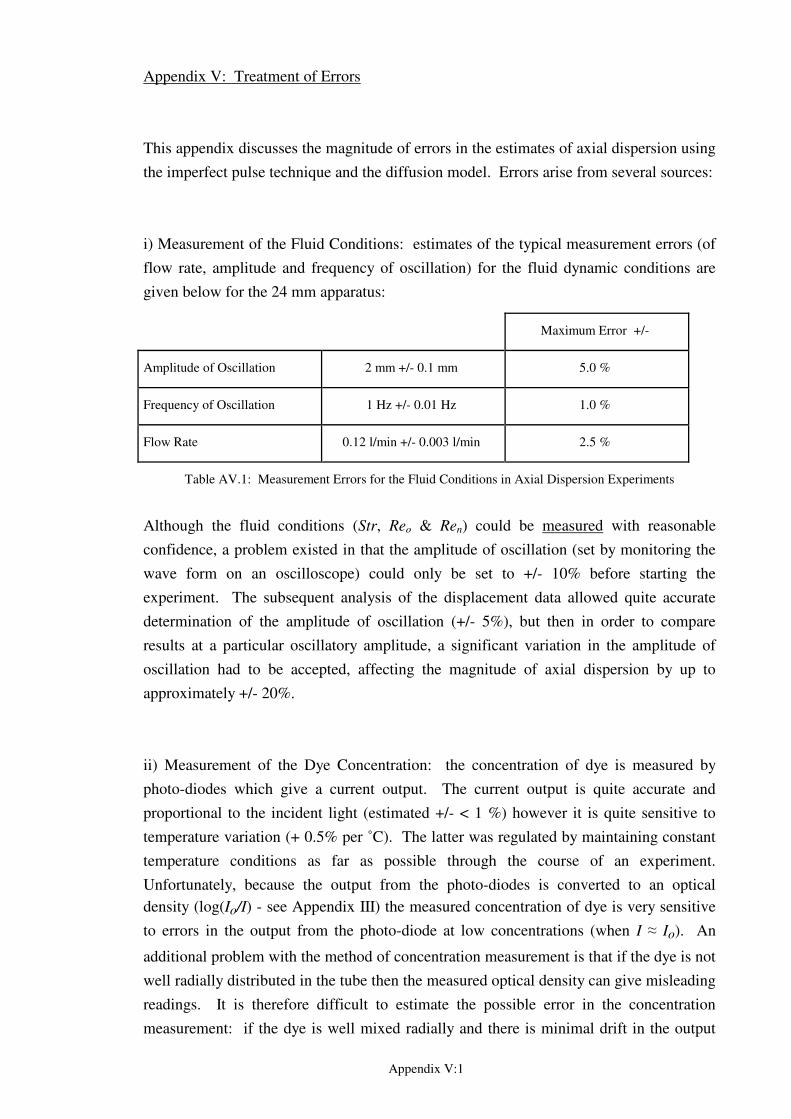
Appendix V:1
Appendix V: Treatment of Errors
This appendix discusses the magnitude of errors in the estimates of axial dispersion using
the imperfect pulse technique and the diffusion model. Errors arise from several sources:
i) Measurement of the Fluid Conditions: estimates of the typical measurement errors (of
flow rate, amplitude and frequency of oscillation) for the fluid dynamic conditions are
given below for the 24 mm apparatus:
Maximum Error +/-
Amplitude of Oscillation 2 mm +/- 0.1 mm 5.0 %
Frequency of Oscillation 1 Hz +/- 0.01 Hz 1.0 %
Flow Rate 0.12 l/min +/- 0.003 l/min 2.5 %
Table AV.1: Measurement Errors for the Fluid Conditions in Axial Dispersion Experiments
Although the fluid conditions (Str, Reo & Ren) could be measured with reasonable
confidence, a problem existed in that the amplitude of oscillation (set by monitoring the
wave form on an oscilloscope) could only be set to +/- 10% before starting the
experiment. The subsequent analysis of the displacement data allowed quite accurate
determination of the amplitude of oscillation (+/- 5%), but then in order to compare
results at a particular oscillatory amplitude, a significant variation in the amplitude of
oscillation had to be accepted, affecting the magnitude of axial dispersion by up to
approximately +/- 20%.
ii) Measurement of the Dye Concentration: the concentration of dye is measured by
photo-diodes which give a current output. The current output is quite accurate and
proportional to the incident light (estimated +/- < 1 %) however it is quite sensitive to
temperature variation (+ 0.5% per ˚C). The latter was regulated by maintaining constant
temperature conditions as far as possible through the course of an experiment.
Unfortunately, because the output from the photo-diodes is converted to an optical
density (log(Io/I) - see Appendix III) the measured concentration of dye is very sensitive
to errors in the output from the photo-diode at low concentrations (when I ≈ Io). An
additional problem with the method of concentration measurement is that if the dye is not
well radially distributed in the tube then the measured optical density can give misleading
readings. It is therefore difficult to estimate the possible error in the concentration
measurement: if the dye is well mixed radially and there is minimal drift in the output
Appendix V:2
from the photo-diode then the results are quite accurate (+/- < 1 %); if on the other hand
the dye is not well mixed (for example laminar creeping flow with central coring of the
flow between the baffles) and the concentrations of dye give a low change in output from
the photo-diodes then the errors are potentially large.
It was therefore considered important to adjust the concentration of the injected pulse of
dye in order to maximise the overall accuracy of the concentration measurements. A
compromise had to be made: if the dye is too dilute then the difference between I and Io
is small and the errors in the calculated optical density are large; if on the other hand the
dye is too concentrated then no light passes through the tube and I tends to zero, causing
inaccurate estimates of the concentration.
iii) The Diffusion Model Analysis: having obtained concentration-time profiles from
dye-tracer experiments the best fit value of axial dispersion E was found by trial and
error: the value of the axial dispersion was adjusted until by inspection the best fit was
obtained between the experimental concentration-time profile and the diffusion model
predicted concentration-time profile. This was considered to be the quickest and most
reliable method of determining E: the alternative used by other researchers was a
numerical least-squares best fit criterion, but this is affected by stray data points (for
example a spike due to a gas bubble passing the optical sensor) and is also sensitive to
the larger errors in measured concentration when the concentration approaches zero
towards the end of an experiment (see above). Determination of the best fit value of
axial dispersion E using the inspection method was found to give a resolution of results
for a given experiment of +/- 10%.
SUMMARY:
Where axial dispersion data is presented on a graph for a particular Strouhal number, the
measured amplitude of oscillation may in fact vary considerably (+/- 10%) from the
nominal Str, with a highly non-linear effect on axial dispersion. This gives an additional
estimated error of up to +/- 20 % when comparing results at a specified Strouhal number.
Combined with the variation due to amplitude measurement (5%) and the diffusion
model analysis (10%) the total error is therefore estimated to be 52
+102
+ 202
≈ 25% .
At very low oscillatory or net flow Reynolds numbers, high Strouhal numbers, or where
radial distribution of the dye tracer is poor, the overall error in measured axial dispersion
may be considerably greater than 25%. The error in the measured Reo is approximately
+/- 5% and about +/- 2.5% for Ren.

Appendix V:3
Errors in the estimates of axial dispersion made using the fluid mechanical simulation
were estimated to be less than 5% so long as the mean rate of increase of particle
variance with time was constant.
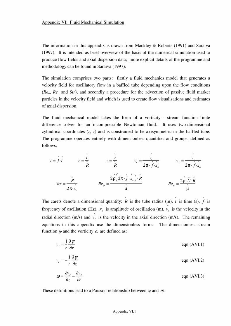
Appendix VI.1
Appendix VI: Fluid Mechanical Simulation
The information in this appendix is drawn from Mackley & Roberts (1991) and Saraiva
(1997). It is intended as brief overview of the basis of the numerical simulation used to
produce flow fields and axial dispersion data; more explicit details of the programme and
methodology can be found in Saraiva (1997).
The simulation comprises two parts: firstly a fluid mechanics model that generates a
velocity field for oscillatory flow in a baffled tube depending upon the flow conditions
(Ren, Reo and Str), and secondly a procedure for the advection of passive fluid marker
particles in the velocity field and which is used to create flow visualisations and estimates
of axial dispersion.
The fluid mechanical model takes the form of a vorticity - stream function finite
difference solver for an incompressible Newtonian fluid. It uses two-dimensional
cylindrical coordinates (r, z) and is constrained to be axisymmetric in the baffled tube.
The programme operates entirely with dimensionless quantities and groups, defined as
follows:
t = f^
⋅t^
r =r^
R^ z =
z^
R^ vr =
vr
^
2π⋅ f^
⋅xo
^ vz =v
z
^
2π⋅ f^
⋅xo
^
Str =R^
2π⋅xo
^ Reo =2ρ
^
2π ⋅ f^
⋅xo
^
⋅ R
^
µ^ Ren =
2ρ^
⋅ U^
⋅ R^
µ^
The carets denote a dimensional quantity: R^
is the tube radius (m), t^
is time (s), f^
is
frequency of oscillation (Hz), xo
^
is amplitude of oscillation (m), vr
^
is the velocity in the
radial direction (m/s) and vz
^
is the velocity in the axial direction (m/s). The remaining
equations in this appendix use the dimensionless forms. The dimensionless stream
function ψ and the vorticity ω are defined as:
vz =1
r
∂ψ
∂r eqn (AVI.1)
vr = −1
r
∂ψ
∂z eqn (AVI.2)
ω =∂v
r
∂z−
∂vz
∂r eqn (AVI.3)
These definitions lead to a Poisson relationship between ψ and ω :
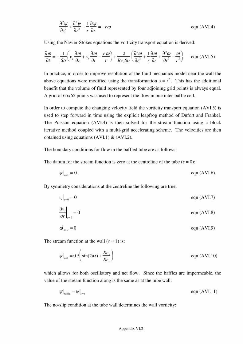
Appendix VI.2
∂2ψ
∂z2 +
∂2ψ
∂r2 −
1
r
∂ψ
∂r= −rω eqn (AVI.4)
Using the Navier-Stokes equations the vorticity transport equation is derived:
∂ω
∂t= −
1
Strvz
∂ω
∂z+ vr
∂ω
∂r−
vrω
r
+2
ReoStr
∂2ω
∂z2 +
1
r
∂ω
∂r+
∂2ω
∂r2 −
ω
r2
eqn (AVI.5)
In practice, in order to improve resolution of the fluid mechanics model near the wall the
above equations were modified using the transformation s = r2
. This has the additional
benefit that the volume of fluid represented by four adjoining grid points is always equal.
A grid of 65x65 points was used to represent the flow in one inter-baffle cell.
In order to compute the changing velocity field the vorticity transport equation (AVI.5) is
used to step forward in time using the explicit leapfrog method of Dufort and Frankel.
The Poisson equation (AVI.4) is then solved for the stream function using a block
iterative method coupled with a multi-grid accelerating scheme. The velocities are then
obtained using equations (AVI.1) & (AVI.2).
The boundary conditions for flow in the baffled tube are as follows:
The datum for the stream function is zero at the centreline of the tube (s = 0):
ψs =0
= 0 eqn (AVI.6)
By symmetry considerations at the centreline the following are true:
vr s= 0= 0 eqn (AVI.7)
∂vz
∂r s= 0
= 0 eqn (AVI.8)
ω s= 0 = 0 eqn (AVI.9)
The stream function at the wall (s = 1) is:
ψs =1
= 0.5 sin(2πt) +Ren
Reo
eqn (AVI.10)
which allows for both oscillatory and net flow. Since the baffles are impermeable, the
value of the stream function along is the same as at the tube wall:
ψbaffle
=ψs =1
eqn (AVI.11)
The no-slip condition at the tube wall determines the wall vorticity:
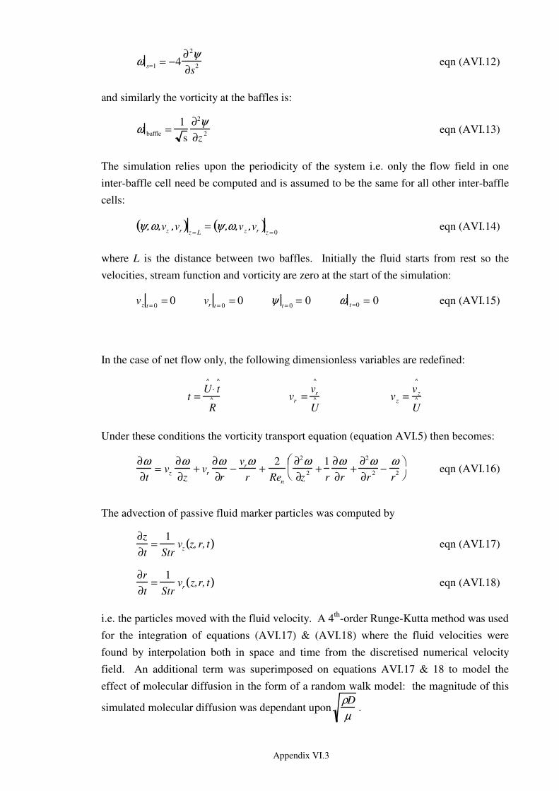
Appendix VI.3
ω s=1 = −4∂ 2ψ
∂s2 eqn (AVI.12)
and similarly the vorticity at the baffles is:
ω baffle =1
s
∂2ψ
∂z2 eqn (AVI.13)
The simulation relies upon the periodicity of the system i.e. only the flow field in one
inter-baffle cell need be computed and is assumed to be the same for all other inter-baffle
cells:
ψ,ω,vz ,vr( )z = L
= ψ,ω,vz ,vr( )z = 0
eqn (AVI.14)
where L is the distance between two baffles. Initially the fluid starts from rest so the
velocities, stream function and vorticity are zero at the start of the simulation:
vz t = 0= 0 vr t = 0
= 0 ψt = 0
= 0 ω t =0 = 0 eqn (AVI.15)
In the case of net flow only, the following dimensionless variables are redefined:
t =U^
⋅ t^
R^ vr =
vr
^
U^ vz =
vz
^
U^
Under these conditions the vorticity transport equation (equation AVI.5) then becomes:
∂ω
∂t= vz
∂ω
∂z+ vr
∂ω
∂r−
vrω
r+
2
Ren
∂2ω
∂z2 +
1
r
∂ω
∂r+
∂2ω
∂r2 −
ω
r2
eqn (AVI.16)
The advection of passive fluid marker particles was computed by
∂z
∂t=
1
Strvz z, r, t( ) eqn (AVI.17)
∂r
∂t=
1
Strvr z,r, t( ) eqn (AVI.18)
i.e. the particles moved with the fluid velocity. A 4th
-order Runge-Kutta method was used
for the integration of equations (AVI.17) & (AVI.18) where the fluid velocities were
found by interpolation both in space and time from the discretised numerical velocity
field. An additional term was superimposed on equations AVI.17 & 18 to model the
effect of molecular diffusion in the form of a random walk model: the magnitude of this
simulated molecular diffusion was dependant uponρD
µ.

Appendix VI.4
Note: the nomenclature in this appendix has been kept consistent with Saraiva (1997),
however some of the symbols used for dimensionless quantities are also used to denote
dimensional quantities elsewhere in this thesis. In order to avoid confusion, the
dimensionless symbols used in this self-contained appendix are not included in the
nomenclature at the end of the thesis.
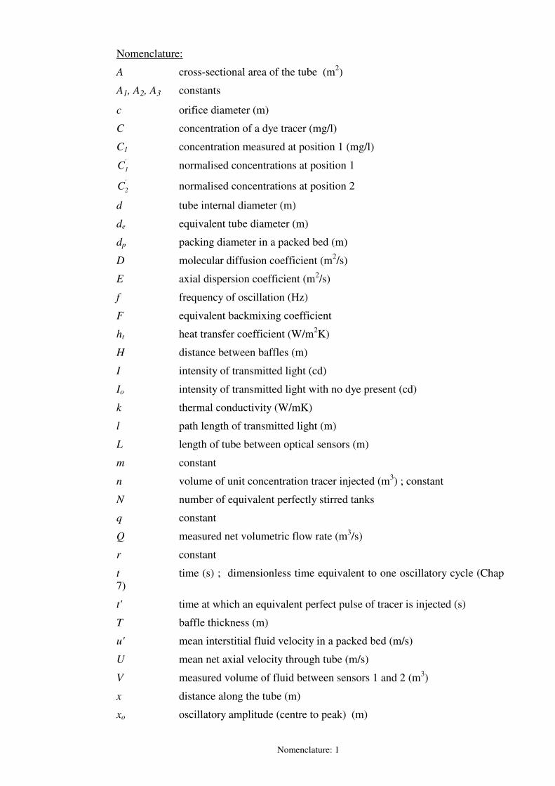
Nomenclature: 1
Nomenclature:
A cross-sectional area of the tube (m2)
A1, A2, A3 constants
c orifice diameter (m)
C concentration of a dye tracer (mg/l)
C1 concentration measured at position 1 (mg/l)
C1
' normalised concentrations at position 1
C2
' normalised concentrations at position 2
d tube internal diameter (m)
de equivalent tube diameter (m)
dp packing diameter in a packed bed (m)
D molecular diffusion coefficient (m2/s)
E axial dispersion coefficient (m2/s)
f frequency of oscillation (Hz)
F equivalent backmixing coefficient
ht heat transfer coefficient (W/m2K)
H distance between baffles (m)
I intensity of transmitted light (cd)
Io intensity of transmitted light with no dye present (cd)
k thermal conductivity (W/mK)
l path length of transmitted light (m)
L length of tube between optical sensors (m)
m constant
n volume of unit concentration tracer injected (m3) ; constant
N number of equivalent perfectly stirred tanks
q constant
Q measured net volumetric flow rate (m3/s)
r constant
t time (s) ; dimensionless time equivalent to one oscillatory cycle (Chap
7)
t' time at which an equivalent perfect pulse of tracer is injected (s)
T baffle thickness (m)
u' mean interstitial fluid velocity in a packed bed (m/s)
U mean net axial velocity through tube (m/s)
V measured volume of fluid between sensors 1 and 2 (m3)
x distance along the tube (m)
xo oscillatory amplitude (centre to peak) (m)
Nomenclature: 2
Greek Symbols:
δ Dirac delta function
∆t short time interval (s)
ε extinction coefficient of methylene blue dye (m2/kg)
εv power density (W/m3)
µ viscosity of fluid (Ns/m2)
ω angular velocity of oscillation (rad/s)
ρ density of fluid (kg/m3)
σ2 variance of particle or concentration distribution (units of m
2 in eqn 6.1,
otherwise dimensionless)
Dimensionless Groups:
Str =d
4πxo
Strouhal number
Reo =ρωxod
µ Oscillatory Reynolds number
Ren =ρUd
µ Net flow Reynolds number
Pe =UL
E Peclet number
Sc =
µ
ρE Schmidt number
Nut =htd
k Tube side Nusselt Number
θ =tU
L dimensionless time