Embed Size (px)
Citation preview
The Science and Technology of Rubber
Fourth Edition
Burak ErmanDepartment of Chemical and Biological Engineering
Koc UniversityRumeli Feneri Yolu 34450 Istanbul, Turkey
James E. MarkDepartment of Chemistry
University of CincinnatiCincinnati, OH 45221-0172, USA
C. Michael RolandNaval Research Laboratory
Chemistry Division, Code 6120Washington, DC, USA
AMSTERDAM • BOSTON • HEIDELBERG • LONDONNEW YORK • OXFORD • PARIS • SAN DIEGO
SAN FRANCISCO • SINGAPORE • SYDNEY • TOKYO
Academic Press is an Imprint of Elsevier
Edited by
Academic Press is an imprint of Elsevier225 Wyman Street, Waltham, MA 02451, USAThe Boulevard, Langford Lane, Kidlington, Oxford, OX5 1GB, UK
© 2013 Elsevier Inc. All rights reserved.
No part of this publication may be reproduced or transmitted in any form or by any means, electronic or mechanical, including photocopying, recording, or any information storage and retrieval system, without permission in writing from the publisher. Details on how to seek permission, further information about the Publisher’s permissions policies and our arrangements with organizations such as the Copyright Clearance Center and the Copyright Licensing Agency, can be found at our website: www.elsevier.com/permissions.
This book and the individual contributions contained in it are protected under copyright by the Publisher (other than as may be noted herein).
NoticesKnowledge and best practice in this field are constantly changing. As new research and experience broaden our understanding, changes in research methods, professional practices, or medical treatment may become necessary.
Practitioners and researchers must always rely on their own experience and knowledge in evaluating and using any information, methods, compounds, or experiments described herein. In using such information or methods they should be mindful of their own safety and the safety of others, including parties for whom they have a professional responsibility.
To the fullest extent of the law, neither the Publisher nor the authors, contributors, or editors, assume any liability for any injury and/or damage to persons or property as a matter of products liability, negligence or otherwise, or from any use or operation of any methods, products, instructions, or ideas contained in the material herein.
Library of Congress Cataloging-in-Publication DataA catalog record for this book is available from the Library of Congress
British Library Cataloguing-in-Publication DataA catalogue record for this book is available from the British Library.
ISBN: 978-0-12-394584-6
Printed in the United States of America13 14 15 9 8 7 6 5 4 3 2 1
For information on all Academic Press publications visit our website at http://store.elsevier.com
Chapter 6
Rheological Behavior andProcessing of UnvulcanizedRubber
C.M RolandChemistry Division, Naval Research Laboratory, Washington, DC, USA
6.1 RHEOLOGY
6.1.1 Introduction
The mixing and processing of rubber is centrally important to achieving usefulproducts at acceptable cost. Various texts review the general topic of polymerprocessing (Osswald and Gries, 2006; Baird and Collias, 1998; Morton-Jones,1989; Tadmor and Gogos, 2006) and the rheology and viscoelasticity of rubberypolymers (Roland, 2011; Macosko, 1994; Ferry, 1980; Watanabe, 1999; Berry,2003; Graessley, 2008), including some specific to rubber processing (White,1995; Johnson, 2001). This chapter provides a basic overview of the rheology(from the Greek rheos, meaning stream or flow, rheology is the study of thedeformation and flow of matter) and processing of uncured rubber, includingrecent developments concerning the material behavior.
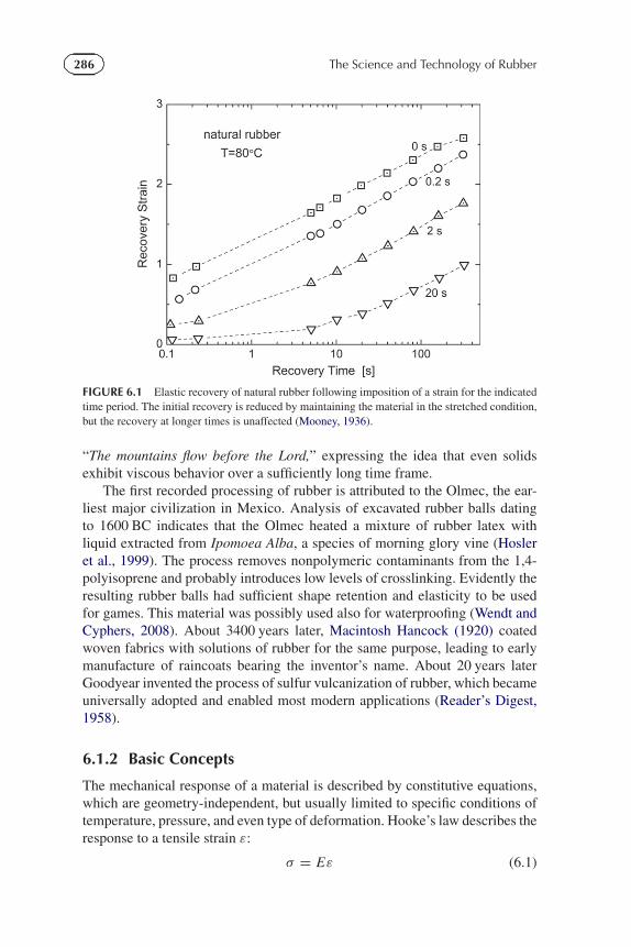
The study of the rheology and processing of rubber had its beginningswith the development of the industry in the early 19th century (Hancock,1920). A major advance was the Boltzmann superposition principle (Boltzmann,1874) (Section 6.2.2), enabling prediction of stresses in a material subjectedto arbitrary strain histories. Early elastic recoil data of Mooney on naturalrubber (Mooney, 1936) are displayed in Figure 6.1, illustrating the Boltzmannsuperpositioning: A short time delay in the onset of recovery only affectsthe recovery at short times; the behavior over longer times is essentially thesame. The first experimental measurements of viscoelastic behavior were onsilk thread, carried out in the mid-19th century (Weber, 1835), although thereis an oblique reference to the concept in the biblical book of Judges 5:5,
The Science and Technology of Rubber. http://dx.doi.org/10.1016/B978-0-12-394584-6.00006-6© 2013 Elsevier Inc. All rights reserved. 285
286 The Science and Technology of Rubber
FIGURE 6.1 Elastic recovery of natural rubber following imposition of a strain for the indicatedtime period. The initial recovery is reduced by maintaining the material in the stretched condition,but the recovery at longer times is unaffected (Mooney, 1936).
“The mountains flow before the Lord,” expressing the idea that even solidsexhibit viscous behavior over a sufficiently long time frame.
The first recorded processing of rubber is attributed to the Olmec, the ear-liest major civilization in Mexico. Analysis of excavated rubber balls datingto 1600 BC indicates that the Olmec heated a mixture of rubber latex withliquid extracted from Ipomoea Alba, a species of morning glory vine (Hosleret al., 1999). The process removes nonpolymeric contaminants from the 1,4-polyisoprene and probably introduces low levels of crosslinking. Evidently theresulting rubber balls had sufficient shape retention and elasticity to be usedfor games. This material was possibly used also for waterproofing (Wendt andCyphers, 2008). About 3400 years later, Macintosh Hancock (1920) coatedwoven fabrics with solutions of rubber for the same purpose, leading to earlymanufacture of raincoats bearing the inventor’s name. About 20 years laterGoodyear invented the process of sulfur vulcanization of rubber, which becameuniversally adopted and enabled most modern applications (Reader’s Digest,1958).
6.1.2 Basic Concepts
The mechanical response of a material is described by constitutive equations,which are geometry-independent, but usually limited to specific conditions oftemperature, pressure, and even type of deformation. Hooke’s law describes theresponse to a tensile strain ε:
σ = Eε (6.1)
287CHAPTER | 6 Rheological Behavior and Processing of Unvulcanized Rubber
in which σ is the stress and E is a material constant known as Young’s modulus.For a strictly elastic material, the behavior is reversible. The behavior of shearedfluids can be described by an equation due to Newton:
σ = ηε (6.2)
in which σ is the shear stress and ε represents the rate of shear or the sheargradient. The proportionality constant in Eq. (6.2) is the viscosity, which is amaterial constant for simple liquids.
Before proceeding, some definitions are useful. Stress is the ratio of the forceon a body to the cross-sectional area of the body. The true stress refers to theinfinitesimal force per (instantaneous) area, while the engineering stress is theforce per initial area. Strain is a measure of the extent of the deformation. Normalstrains change the dimensions, whereas shear strains change the angle betweentwo initially perpendicular lines. In correspondence with the true stress, theCauchy (or Euler) strain is measured with respect to the deformed state, whilethe Green’s (or Lagrange) strain is with respect to the undeformed state.
The simple form of Eqs. (6.1) and (6.2) embodies two assumptions. Thematerial is isotropic, so that the properties are the same in all directions. Moregenerally, the stress is a tensor
σi j =⎛⎜⎝σ11 σ12 σ13
σ21 σ22 σ23
σ31 σ32 σ33
⎞⎟⎠ (6.3)
in which the subscripts refer to the rectilinear coordinates. To avoid rotationor translation of a body, σ12 = σ21, σ13 = σ31, and so on; thus, only six ofthe stress components are unique. The set of axes for which one of the normalstresses is maximum defines the principal stresses
σi j =⎛⎜⎝σ11 0 0
0 σ22 0
0 0 σ33
⎞⎟⎠ . (6.4)
These can be found as roots of the equation
σ 3 − I1σ2 − I2σ − I3 = 0 (6.5)
in which I1, I2, and I3 are the so-called strain invariants,
I1 = λ21 + λ2
2 + λ23, I2 = λ2
1λ22 + λ2
1λ23 + λ2
2λ23, I3 = λ2
1λ22λ
23. (6.6)
Strain invariants are independent of the axes used to define the geometry,enabling calculations for inhomogeneous deformations without explicitconsideration of the principal directions. During a homogenous deformation,
288 The Science and Technology of Rubber�
�
�
�
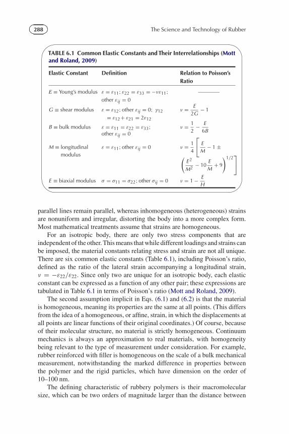
TABLE 6.1 Common Elastic Constants and Their Interrelationships (Mottand Roland, 2009)
Elastic Constant Definition Relation to Poisson’sRatio
E ≡ Young’s modulus ε = ε11; ε22 = ε33 = −νε11; ————
other εij = 0
G ≡ shear modulus ε = ε12; other εij = 0; γ12 ν = E2G
− 1= ε12+ ε21 = 2ε12
B ≡ bulk modulus ε = ε11 = ε22 = ε33;other εij = 0
ν = 12
− E6B
M ≡ longitudinal ε = ε11; other εij = 0 ν = 14
⎡⎣ E
M− 1 ±
modulus (E2
M2 − 10EM
+ 9
)1/2⎤⎦
E ≡ biaxial modulus σ = σ11 = σ22; other σij = 0 ν = 1 − EH
parallel lines remain parallel, whereas inhomogeneous (heterogeneous) strainsare nonuniform and irregular, distorting the body into a more complex form.Most mathematical treatments assume that strains are homogeneous.
For an isotropic body, there are only two stress components that areindependent of the other. This means that while different loadings and strains canbe imposed, the material constants relating stress and strain are not all unique.There are six common elastic constants (Table 6.1), including Poisson’s ratio,defined as the ratio of the lateral strain accompanying a longitudinal strain,ν = −ε22/ε22. Since only two are unique for an isotropic body, each elasticconstant can be expressed as a function of any other pair; these expressions aretabulated in Table 6.1 in terms of Poisson’s ratio (Mott and Roland, 2009).
The second assumption implicit in Eqs. (6.1) and (6.2) is that the materialis homogeneous, meaning its properties are the same at all points. (This differsfrom the idea of a homogeneous, or affine, strain, in which the displacements atall points are linear functions of their original coordinates.) Of course, becauseof their molecular structure, no material is strictly homogeneous. Continuummechanics is always an approximation to real materials, with homogeneitybeing relevant to the type of measurement under consideration. For example,rubber reinforced with filler is homogeneous on the scale of a bulk mechanicalmeasurement, notwithstanding the marked difference in properties betweenthe polymer and the rigid particles, which have dimension on the order of10–100 nm.
The defining characteristic of rubbery polymers is their macromolecularsize, which can be two orders of magnitude larger than the distance between
289CHAPTER | 6 Rheological Behavior and Processing of Unvulcanized Rubber
atoms. As a result, internal motions occur over a range of length scales, eachassociated with a different time scale. This means that whether an externalperturbation is “slow” or “fast” depends on the mode of motion it excites.Invariably, some modes move on the time scale of the perturbation, dissipatingenergy and causing a peak in the out-of-phase, or loss, component of thedynamic response, at a frequency equal to that of the underlying motion.Other modes, such as vibrations, are relatively fast, responding elastically,or they involve the entire molecule, manifested as flow (in the absence of anetwork structure). If the time scale of the motion is very long, the mode can beunresponsive to the perturbation; a well-known example is the conformationaltransitions of a polymer backbone below the glass transition temperature. Thenet effect of this diversity of modes of motion is a frequency-dependent responseto mechanical excitation, or equivalently, a time-varying reaction to a transientperturbation. This means that elastic constants such as E or η are not constantfor a viscoelastic material, but vary with dynamic frequency or time.
Although the rheology and processing of rubber entails mechanical proper-ties as described earlier, viscoelasticity encompasses other manifestationsof the same underlying motions, such as dielectric polarization, dynamicbirefringence, and the inelastic scattering of light, X-rays, and neutrons.Viscoelastic materials exhibit a second, related property, the simultaneousstorage and dissipation of energy, from which the term originates. The normalforces accompanying shear flow of polymers are due to the elasticity of thematerial, and hence another manifestation of viscoelasticity.
Viscoelasticity can also be observed in nonpolymeric materials, althoughusually only over a limited range of conditions (whereas polymers have rate-dependent mechanical properties at almost all temperatures). An example isthe viscosity of supercooled molecular liquids (Angell et al., 2000; Rolandet al., 2005). Creep of metals under sustained loading at elevated temperatureis referred to as viscoelasticity (Kennedy, 1953; McLean, 1966), although thebehavior is caused by changes in dislocations or grain size. Strictly speaking,viscoelasticity refers only to the properties of an unchanging material; if thevariation in the response with time is due to changes of the material itself(e.g., the drying of concrete or chain scission in a sheared polymer), this is notviscoelasticity.
6.2 LINEAR VISCOELASTICITY
6.2.1 Material Constants
Due to their viscoelastic nature, the response of polymers depends entirely onthe loading history, and the simple inverse relationship between moduli andcompliances is lost. Thus, Eq. (6.1) for application of a shear strain becomes
G(t) = σ(t)/ε0 (6.7)
290 The Science and Technology of Rubber
in which G(t) is the stress relaxation modulus; tensile stresses would yield thecorresponding tensile relaxation modulus, E(t). Imposing a constant load yieldsthe compliance, which for shear is
J (t) = γ (t)/σ0. (6.8)
The two response functions are related as∫ t
0G(u)J (t − u)du = t (6.9)
but the stress relaxation and compliance are not reciprocals
G(t)J (t) < 1. (6.10)
For a viscoelastic material, the viscosity in the limit of zero-shear rate, theNewtonian viscosity, can be obtained from the integral of the stress relaxationmodulus
η0 =∫ ∞
0G(t)dt =
∫ ∞
0tG(t)d ln t . (6.11)
A logarithmic time axis is necessary because of the very broad time scale of thedynamics of polymers.
The steady-state recoverable compliance, which is a measure of the elasticstrain, can be calculated using
J 0s =
∫ ∞
0tG(t)dt
/(∫ ∞
0G(t)dt
)2
. (6.12)
The compliance function measured in a creep experiment can be decomposedinto recoverable and viscous flow components
J (t) = Jr (t)+ t/η, (6.13)
where Jr (t) is the recoverable compliance. After steady state is attained, andthe viscosity becomes equal to η0,
J 0s = lim
t→∞ Jr (t). (6.14)
The steady-state recoverable compliance can be measured by fitting Eq. (6.13)to creep data at long times, or more accurately, J 0
s is determined from therecovery after removal of the stress subsequent to attainment of steady-stateflow.
The Kramers-Kronig formula relates the stress relaxation modulus todynamic quantities (Kronig, 1926; Kramers, 1927)
∫ ∞
0G ′(ω) sinωt
ωdω =
∫ ∞
0G ′′(ω)cosωt
ωdω = π
2G(t) (6.15)
291CHAPTER | 6 Rheological Behavior and Processing of Unvulcanized Rubber
or the inverse relations for the storage modulus
G ′(ω) = ω
∫ ∞
0G(t) sin (ωt)dt (6.16)
and the loss modulus
G ′′(ω) = ω
∫ ∞
0G(t) cos (ωt)dt . (6.17)
An approximate relation is (Tschoegl, 1989)
G ′′(ω) ≈ π
2
dG ′(ω)d lnω
. (6.18)
An analogous expression for the dielectric loss in terms of the derivative of thepermittivity is commonly used to avoid the problem of dielectric loss peaksbeing masked by dc conductivity (the latter not contributing to the in-phaseresponse) (Wubbenhorst and Van Turnhout, 2002).
The dynamic viscosity, η = G ′′(ω)/ω, yields the terminal viscosity in thelimit of zero frequency
η0 = limω→0
G ′′(ω)/ω (6.19)
and J 0s can be obtained from the zero-shear-rate limiting value of the storage
modulusJ 0
s = η−20 lim
ω→0ω−2G ′(ω). (6.20)
Alternatively, from steady shearing experiments, which yield η0 directly in thelimit of low shear rate, the steady-state recoverable compliance can be obtainedfrom the first normal stress coefficient,0, which is the ratio of the first normalstress difference to the square of the shear rate, measured at low shear rate
J 0s = 0
2η20
. (6.21)
From Eq. (6.12) the steady-state recoverable compliance is also given by
J 0s = η−2
0
∫ ∞
0tG(t)dt . (6.22)
It follows from Eqs. (6.11) and (6.17) that
η0 = limω→0
G ′′(ω)/ω (6.23)
Experimentally steady state in a transient experiment implies
J (t) ∼ t . (6.24)
The steady-state recoverable compliance is an important rheological parameterbecause it is very sensitive to the high molecular tail of the molecular weightdistribution, and thus can be correlated with elastic properties of a rubber.
292 The Science and Technology of Rubber
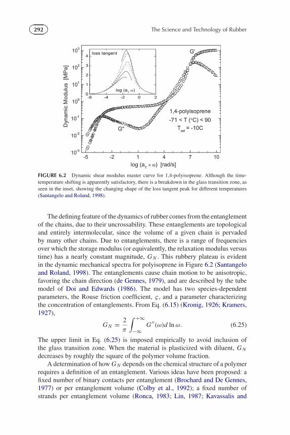
FIGURE 6.2 Dynamic shear modulus master curve for 1,4-polyisoprene. Although the time-temperature shifting is apparently satisfactory, there is a breakdown in the glass transition zone, asseen in the inset, showing the changing shape of the loss tangent peak for different temperatures(Santangelo and Roland, 1998).
The defining feature of the dynamics of rubber comes from the entanglementof the chains, due to their uncrossability. These entanglements are topologicaland entirely intermolecular, since the volume of a given chain is pervadedby many other chains. Due to entanglements, there is a range of frequenciesover which the storage modulus (or equivalently, the relaxation modulus versustime) has a nearly constant magnitude, G N . This rubbery plateau is evidentin the dynamic mechanical spectra for polyisoprene in Figure 6.2 (Santangeloand Roland, 1998). The entanglements cause chain motion to be anisotropic,favoring the chain direction (de Gennes, 1979), and are described by the tubemodel of Doi and Edwards (1986). The model has two species-dependentparameters, the Rouse friction coefficient, ς , and a parameter characterizingthe concentration of entanglements. From Eq. (6.15) (Kronig, 1926; Kramers,1927),
G N = 2
π
∫ +∞
−∞G ′′(ω)d lnω. (6.25)
The upper limit in Eq. (6.25) is imposed empirically to avoid inclusion ofthe glass transition zone. When the material is plasticized with diluent, G N
decreases by roughly the square of the polymer volume fraction.A determination of how G N depends on the chemical structure of a polymer
requires a definition of an entanglement. Various ideas have been proposed: afixed number of binary contacts per entanglement (Brochard and De Gennes,1977) or per entanglement volume (Colby et al., 1992); a fixed number ofstrands per entanglement volume (Ronca, 1983; Lin, 1987; Kavassalis and
293CHAPTER | 6 Rheological Behavior and Processing of Unvulcanized Rubber
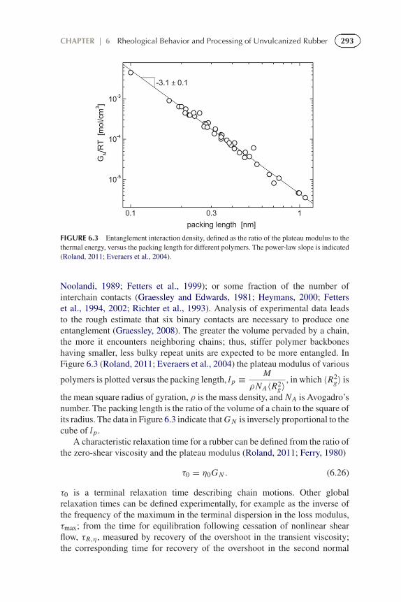
FIGURE 6.3 Entanglement interaction density, defined as the ratio of the plateau modulus to thethermal energy, versus the packing length for different polymers. The power-law slope is indicated(Roland, 2011; Everaers et al., 2004).
Noolandi, 1989; Fetters et al., 1999); or some fraction of the number ofinterchain contacts (Graessley and Edwards, 1981; Heymans, 2000; Fetterset al., 1994, 2002; Richter et al., 1993). Analysis of experimental data leadsto the rough estimate that six binary contacts are necessary to produce oneentanglement (Graessley, 2008). The greater the volume pervaded by a chain,the more it encounters neighboring chains; thus, stiffer polymer backboneshaving smaller, less bulky repeat units are expected to be more entangled. InFigure 6.3 (Roland, 2011; Everaers et al., 2004) the plateau modulus of various
polymers is plotted versus the packing length, l p ≡ M
ρNA〈R2g〉
, in which 〈R2g〉 is
the mean square radius of gyration, ρ is the mass density, and NA is Avogadro’snumber. The packing length is the ratio of the volume of a chain to the square ofits radius. The data in Figure 6.3 indicate that G N is inversely proportional to thecube of l p.
A characteristic relaxation time for a rubber can be defined from the ratio ofthe zero-shear viscosity and the plateau modulus (Roland, 2011; Ferry, 1980)
τ0 = η0G N . (6.26)
τ0 is a terminal relaxation time describing chain motions. Other globalrelaxation times can be defined experimentally, for example as the inverse ofthe frequency of the maximum in the terminal dispersion in the loss modulus,τmax; from the time for equilibration following cessation of nonlinear shearflow, τR,η, measured by recovery of the overshoot in the transient viscosity;the corresponding time for recovery of the overshoot in the second normal
294 The Science and Technology of Rubber�
�
�
�
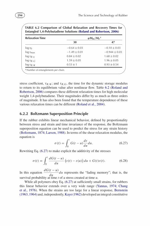
TABLE 6.2 Comparison of Global Relaxation and Recovery Times forEntangled 1,4-Polybutadiene Solutions (Roland and Robertson, 2006)
Relaxation Time ϕMw /Mea
30 47
log τ0 −0.64 ± 0.03 −0.10 ± 0.03
log τmax −1.49 ± 0.01 −0.944 ± 0.03
log τR ,η 0.84 ± 0.02 1.68 ± 0.02
log τR ,G 1.59 ± 0.05 1.96 ± 0.05
log τR , 0.53 ± 1 0.93 ± 0.54
aNumber of entanglements per chain.
stress coefficient, τR, ; and τR,G , the time for the dynamic storage modulusto return to its equilibrium value after nonlinear flow. Table 6.2 (Roland andRobertson, 2006) compares these different relaxation times for high molecularweight 1,4-polybutadiene. Their magnitudes differ by as much as three ordersof magnitude. It has also been found that the temperature dependence of thesevarious relaxation times can be different (Roland et al., 2004).
6.2.2 Boltzmann Superposition Principle
If the rubber exhibits linear mechanical behavior, defined by proportionalitybetween stress and strain and time invariance of the response, the Boltzmannsuperposition equation can be used to predict the stress for any strain history(Boltzmann, 1874; Larson, 1988). In terms of the shear relaxation modulus, theequation is
σ(t) =∫ t
0G(t − u)
dε
dudu. (6.27)
Rewriting Eq. (6.27) to make explicit the additivity of the stresses
σ(t) =∫ t
0
dG(t − u)
du
(ε(t)− ε(u)
)du + G(t)ε(t). (6.28)
In this equationdG(t − u)
dudu represents the “fading memory”; that is, the
survival probability at time t of a stress created at time u.While all polymers obey Eq. (6.27) at sufficiently small strains, for rubbers
this linear behavior extends over a very wide range (Yannas, 1974; Changet al., 1976). When the strains are too large for a linear response, Bernstein(1963, 1964) and, independently, Kaye (1962) developed an integral constitutive
295CHAPTER | 6 Rheological Behavior and Processing of Unvulcanized Rubber
equation to describe the nonlinear viscoelastic properties, known as the K-BKZequation
σ(t) =∫ t
0[G(t − u,ε(t − u))] dε
dudu. (6.29)
If the relaxation behavior, G(t), in Eq. (6.29) is independent of strain, thebehavior is referred to as “time invariant.” This decoupling of time and straineffects leads to a simpler expression
σ(t) =∫ t
0[G(t − u)g(ε)] dε
dudu. (6.30)
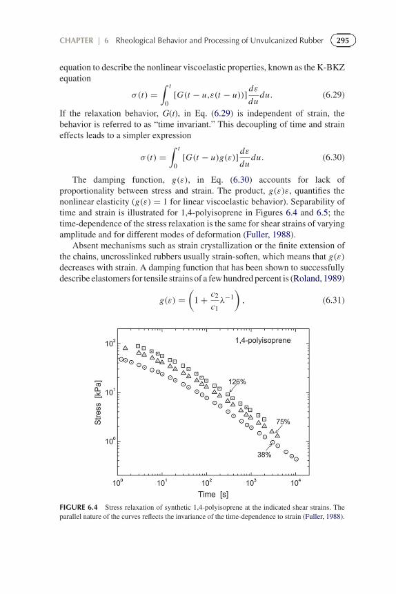
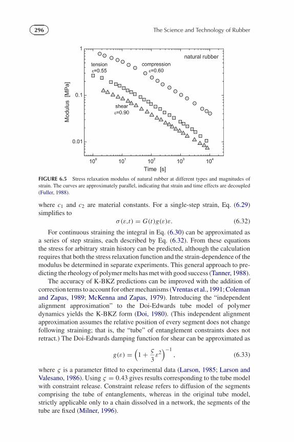
The damping function, g(ε), in Eq. (6.30) accounts for lack ofproportionality between stress and strain. The product, g(ε)ε, quantifies thenonlinear elasticity (g(ε) = 1 for linear viscoelastic behavior). Separability oftime and strain is illustrated for 1,4-polyisoprene in Figures 6.4 and 6.5; thetime-dependence of the stress relaxation is the same for shear strains of varyingamplitude and for different modes of deformation (Fuller, 1988).
Absent mechanisms such as strain crystallization or the finite extension ofthe chains, uncrosslinked rubbers usually strain-soften, which means that g(ε)decreases with strain. A damping function that has been shown to successfullydescribe elastomers for tensile strains of a few hundred percent is (Roland, 1989)
g(ε) =(
1 + c2
c1λ−1
), (6.31)
FIGURE 6.4 Stress relaxation of synthetic 1,4-polyisoprene at the indicated shear strains. Theparallel nature of the curves reflects the invariance of the time-dependence to strain (Fuller, 1988).
296 The Science and Technology of Rubber
FIGURE 6.5 Stress relaxation modulus of natural rubber at different types and magnitudes ofstrain. The curves are approximately parallel, indicating that strain and time effects are decoupled(Fuller, 1988).
where c1 and c2 are material constants. For a single-step strain, Eq. (6.29)simplifies to
σ(ε,t) = G(t)g(ε)ε. (6.32)
For continuous straining the integral in Eq. (6.30) can be approximated asa series of step strains, each described by Eq. (6.32). From these equationsthe stress for arbitrary strain history can be predicted, although the calculationrequires that both the stress relaxation function and the strain-dependence of themodulus be determined in separate experiments. This general approach to pre-dicting the rheology of polymer melts has met with good success (Tanner, 1988).
The accuracy of K-BKZ predictions can be improved with the addition ofcorrection terms to account for other mechanisms (Vrentas et al., 1991; Colemanand Zapas, 1989; McKenna and Zapas, 1979). Introducing the “independentalignment approximation” to the Doi-Edwards tube model of polymerdynamics yields the K-BKZ form (Doi, 1980). (This independent alignmentapproximation assumes the relative position of every segment does not changefollowing straining; that is, the “tube” of entanglement constraints does notretract.) The Doi-Edwards damping function for shear can be approximated as
g(ε) =(
1 + ς
3ε2)−1
, (6.33)
where ς is a parameter fitted to experimental data (Larson, 1985; Larson andValesano, 1986). Using ς = 0.43 gives results corresponding to the tube modelwith constraint release. Constraint release refers to diffusion of the segmentscomprising the tube of entanglements, whereas in the original tube model,strictly applicable only to a chain dissolved in a network, the segments of thetube are fixed (Milner, 1996).
297CHAPTER | 6 Rheological Behavior and Processing of Unvulcanized Rubber
6.2.3 Time-Temperature Equivalence
Most mechanical test instruments have a limited dynamic range, typically downto ca. 10−4 s−1 for low strain rates, which almost always requires transientmeasurements, and up to about 100 s−1 on the high frequency end, usuallyemploying dynamic measurements. Servohydraulic test systems can achievehigher speeds, but with limitations on the attainable strains (Bergstrom andBoyce, 1998; Arruda et al., 2001). If only the linear viscoelastic response is tobe measured, dielectric spectroscopy (Kremer and Schonhals, 2003; McCrumet al., 1967) can be used. Dielectric spectroscopy can be carried out routinelyover 11 decades of frequency, extending to GHz; this range can be extendedto as much as 18 decades (Schneider et al., 1999), although this requirescorrections be made for effects from the connectors and cables. However,dielectric relaxation only probes the local segmental dynamics of polymers,except for the few cases in which a dipole moment is present parallel to thepolymer chain. For the latter the chain modes are dielectrically active, and thedynamics of the chain end-to-end vector can be measured. Although dielectricrelaxation times are smaller than the corresponding mechanical relaxations,their respective dependences on temperature (Boese et al., 1989; Colmeneroet al., 1991, 1994; Paluch et al., 2002, 2003) and pressure (Bair and Winer, 1980;Roland et al., 2006) are the same. Another advantage of dielectric spectroscopyis the relative ease of obtaining measurements at elevated hydrostatic pressure(Roland et al., 2005; Skorodumov and Godovskii, 1993; Floudas, 2003). Fewmechanical studies of the effect of pressure have been carried out, and theseare usually limited to studying the viscosity of low molecular weight polymers(Hellwege et al., 1967; Fillers and Tschoegl, 1977; Bair, 2002). The dynamicmodulus of polymer melts can be measured in a rheometer pressurized with agas (Han and Ma, 1983; Gerhardt et al., 1997; Royer et al., 2000), but sincegases dissolve in the material, the consequent plasticization can introduce error.
(i) Superposition PrincipleThe most common means to extend the frequency scale is to invoke time-temperature superpositioning (Ferry, 1980). If all motions of a polymercontributing to a particular viscoelastic response are affected the same bytemperature, then changes in temperature only alter the overall time scale; sucha material is thermorheologically simple. Thermorheological simplicity meansconformance to the time-temperature superposition principle, whereby lowerand higher strain rate data can be obtained from measurements at higher andlower temperatures, respectively.
Time-temperature superpositioning was originally derived from free vol-ume models, which assume that the rates of molecular motions are governedby the available unoccupied space. Early studies of molecular liquids led tothe Doolittle equation, relating the viscosity to the fractional free volume,f (≡V /(V − V0), where V is the specific volume and V0 is the occupied volumenormalized by the mass) (Doolittle and Doolittle, 1957; Cohen and Turnbull,
298 The Science and Technology of Rubber
1959):log η(T ) = log AD + BD/ f (T ), (6.34)
with AD and BD constants. However, Eq. (6.34) only approximately fits exper-imental data (Corezzi et al., 1999; Paluch, 2001; Schug et al., 1998). The
assumption that the free volume expands linearly with temperature,d f
dT
∣∣∣∣P
∼ T ,
leads to the Williams-Landel-Ferry (WLF) equation (Ferry, 1980; Williamset al., 1955):
log a(T ) = log a(TR)− c1(T − TR)
c2 + T − TR, (6.35)
where TR is an arbitrary reference temperature. Assuming the WLF constants c1and c2 are functions of the free volume leads to “universal values” of c1 = 8.86and c2 = 101.6 (Williams et al., 1955). In Eq. (6.35) a(T ) is a time-temperatureshift factor, defined for the viscosity as a(T ) = η(T )/η(TR), or for the relax-ation times as a(T ) = τ(T )/τ (TR). (η and τ are proportional except near theglass transition (Chang and Sillescu, 1997; Rössler, 1990; Fischer et al., 1992);cf. Eq. (6.26).) Shift factors are used because the actual magnitude of the vis-coelastic quantities does not affect t−T superpositioning, only their change withtemperature. An ostensibly different, but mathematically equivalent expressionto Eq. (6.35) is due to Vogel, Fulcher, Tamman, and Hesse (Ferry, 1980):
log τ(T ) = log τ∞ + bVFTH
T − TV, (6.36)
in which bVFTH (=c1/c2), TV (=TR −c2), and τ∞ are constants (Zallen, 1981).At the Vogel temperature, TV , the dynamics would diverge if not for interven-tion of the glass transition. TV is often taken to be the Kauzmann temperature atwhich the extrapolated liquid entropy equals the crystal entropy, ostensibly inviolation of the third law of thermodynamics (“Kauzmann paradox”) (Angell,1991).
Cohen and Grest (1979, 1984) and Grest and Cohen (1981) derived a morerigorous free volume model, in which molecules have mobility only when localcontinuity of empty space exists. Generally free volume models have fallen intodisfavor, due to the unphysical results they lead to; for example, free volumescan become negative (Williams and Angell, 1977) or change less with pressurethan the occupied volume (Ferry, 1980). Nevertheless, Eqs. (6.35) or (6.36) canstill be used to fit experimental data. However, the absence of a firm theoreticalfoundation means that the validity of time-temperature superpositioning mustbe established empirically for any material. A major development in the studyof polymer viscoelasticity was in 1949, when samples of a high molecularweight polyisobutylene were distributed to laboratories around the world. Bothtransient, in particular stress relaxation measurements (Andrews and Tobolsky,1951), and dynamic experiments (Fitzgerald et al., 1953; Ferry et al., 1953) werecarried out, with the data spanning 15 decades of frequency. The successful
299CHAPTER | 6 Rheological Behavior and Processing of Unvulcanized Rubber
superpositioning of these results led to the acceptance of time-temperaturesuperpositioning as a method of converting viscoelastic data for polymersobtained over a narrow dynamic range to master curves covering many decadesof reduced time or frequency (Roland, 2011; Ferry, 1980; Marvin, 1953).
The four requirements for thermorheological simplicity are:
● The local friction coefficient is the same for all motions underlying theviscoelastic property of interest.
● The polymer does not degrade, crystallize, physically age, or undergo otherchanges over the course of the measurements.
● At high strain rates, the deformation period is not less than the time requiredfor stress waves to travel through the material; this ensures spatial uniformityof the stress.
● Heat build-up, more pronounced for low temperatures and high rates, causesno deviation from isothermal conditions.
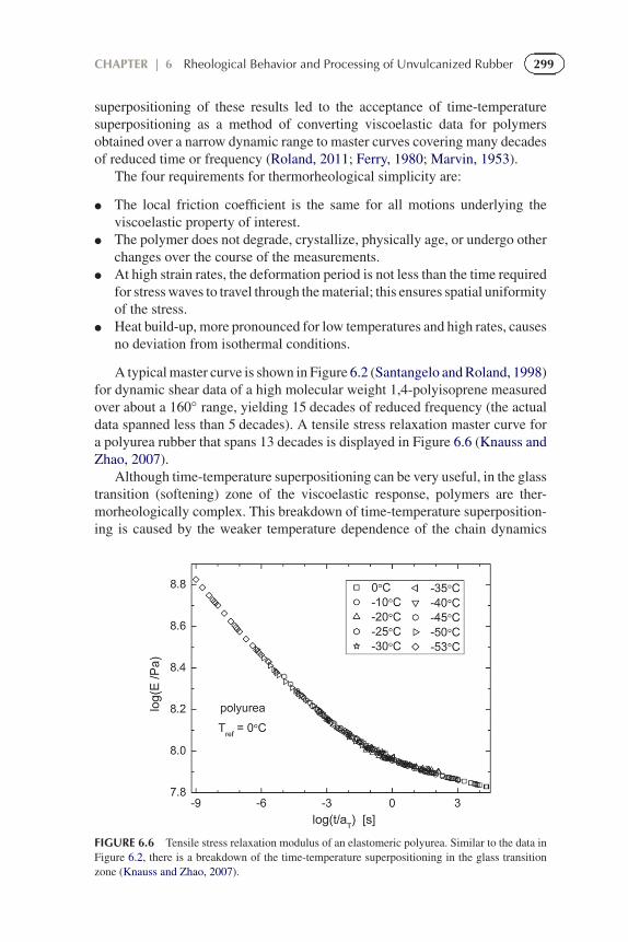
A typical master curve is shown in Figure 6.2 (Santangelo and Roland, 1998)for dynamic shear data of a high molecular weight 1,4-polyisoprene measuredover about a 160◦ range, yielding 15 decades of reduced frequency (the actualdata spanned less than 5 decades). A tensile stress relaxation master curve fora polyurea rubber that spans 13 decades is displayed in Figure 6.6 (Knauss andZhao, 2007).
Although time-temperature superpositioning can be very useful, in the glasstransition (softening) zone of the viscoelastic response, polymers are ther-morheologically complex. This breakdown of time-temperature superposition-ing is caused by the weaker temperature dependence of the chain dynamics
FIGURE 6.6 Tensile stress relaxation modulus of an elastomeric polyurea. Similar to the data inFigure 6.2, there is a breakdown of the time-temperature superpositioning in the glass transitionzone (Knauss and Zhao, 2007).
300 The Science and Technology of Rubber
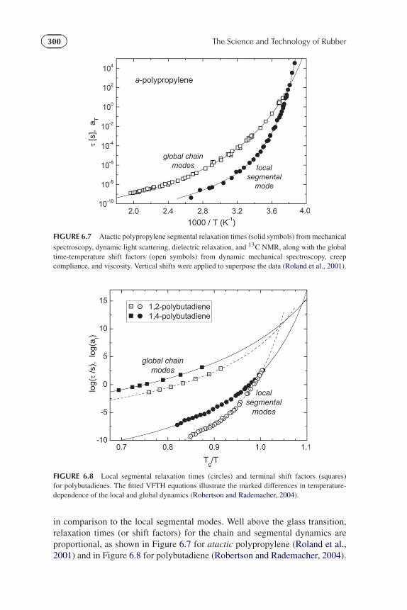
FIGURE 6.7 Atactic polypropylene segmental relaxation times (solid symbols) from mechanical
spectroscopy, dynamic light scattering, dielectric relaxation, and 13C NMR, along with the globaltime-temperature shift factors (open symbols) from dynamic mechanical spectroscopy, creepcompliance, and viscosity. Vertical shifts were applied to superpose the data (Roland et al., 2001).
FIGURE 6.8 Local segmental relaxation times (circles) and terminal shift factors (squares)for polybutadienes. The fitted VFTH equations illustrate the marked differences in temperature-dependence of the local and global dynamics (Robertson and Rademacher, 2004).
in comparison to the local segmental modes. Well above the glass transition,relaxation times (or shift factors) for the chain and segmental dynamics areproportional, as shown in Figure 6.7 for atactic polypropylene (Roland et al.,2001) and in Figure 6.8 for polybutadiene (Robertson and Rademacher, 2004).
301CHAPTER | 6 Rheological Behavior and Processing of Unvulcanized Rubber
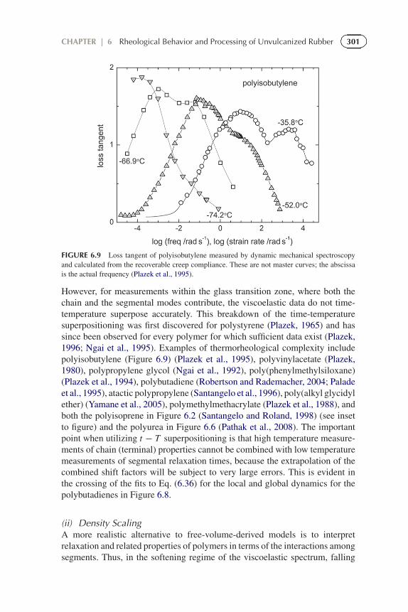
FIGURE 6.9 Loss tangent of polyisobutylene measured by dynamic mechanical spectroscopyand calculated from the recoverable creep compliance. These are not master curves; the abscissais the actual frequency (Plazek et al., 1995).
However, for measurements within the glass transition zone, where both thechain and the segmental modes contribute, the viscoelastic data do not time-temperature superpose accurately. This breakdown of the time-temperaturesuperpositioning was first discovered for polystyrene (Plazek, 1965) and hassince been observed for every polymer for which sufficient data exist (Plazek,1996; Ngai et al., 1995). Examples of thermorheological complexity includepolyisobutylene (Figure 6.9) (Plazek et al., 1995), polyvinylacetate (Plazek,1980), polypropylene glycol (Ngai et al., 1992), poly(phenylmethylsiloxane)(Plazek et al., 1994), polybutadiene (Robertson and Rademacher, 2004; Paladeet al., 1995), atactic polypropylene (Santangelo et al., 1996), poly(alkyl glycidylether) (Yamane et al., 2005), polymethylmethacrylate (Plazek et al., 1988), andboth the polyisoprene in Figure 6.2 (Santangelo and Roland, 1998) (see insetto figure) and the polyurea in Figure 6.6 (Pathak et al., 2008). The importantpoint when utilizing t − T superpositioning is that high temperature measure-ments of chain (terminal) properties cannot be combined with low temperaturemeasurements of segmental relaxation times, because the extrapolation of thecombined shift factors will be subject to very large errors. This is evident inthe crossing of the fits to Eq. (6.36) for the local and global dynamics for thepolybutadienes in Figure 6.8.
(ii) Density ScalingA more realistic alternative to free-volume-derived models is to interpretrelaxation and related properties of polymers in terms of the interactions amongsegments. Thus, in the softening regime of the viscoelastic spectrum, falling
302 The Science and Technology of Rubber
intermediate to the rubbery and glassy plateaus, the polymer dynamics entailsjumps over potential barriers that are large compared to the available thermalenergy (Goldstein, 1969; Stillinger and Weber, 1984; Sampoli et al., 2003).The dense packing at lower temperatures, however, means that the segmentaldynamics are correlated—motion of a given segment occurs in cooperativefashion with neighboring segments. This interpretation of the dynamics requiresconsideration of the nature of the intermolecular potential governing thesereciprocal interactions among segments. A simplified potential that considersonly two-body interactions is the symmetric Lennard-Jones (LJ) potentialenergy function
U (r) = 4ε[(r0/r)
12 − (r0/r)6], (6.37)
where ε is a measure of the depth of the potential well and r the separationbetween segments (which are taken to be spherical particles of radius r0). Theattractive term in this equation has an exponent equal to six because only vander Waals dispersion interactions are considered. The repulsive forces have astronger dependence on particle separation than the attractive forces; moreover,unlike van der Waals forces, the distance dependence varies with chemicalstructure (Moelwyn-Hughes, 1961; Bardik and Sysoev, 1998). A more realisticform of the LJ function is then
U (r) = 4ε[(r0/r)
m − (r0/r)6], (6.38)
where the value of m depends on the species.If the primary focus is on the segmental dynamics and properties involving
local interactions, the attractive forces can be ignored, since they are long rangedand tend to cancel locally (Widen, 1967; Chandler et al., 1983; Stillinger et al.,2001). This follows from the fact that the force on a segment is the vector sumof all forces from neighboring segments, and there are many such neighbors(Widom, 1999). Thus, an approximate form for the potential can be assumed(Hansen, 1970; March and Tosi, 2002):
U (r) = ε(r0/r)m . (6.39)
This inverse power law (IPL) neglects attractive forces, consistent with thefact that the liquid structure is determined primarily by packing effects, whichdepend only on the repulsions (Hoover and Ross, 1971; Laird and Haymet,1992). If an IPL accurately represents the local interaction energy betweensegments, then all thermodynamic properties (such as the energy, volume, andentropy) (March and Tosi, 2002; Hoover and Ross, 1971), as well as dynamicproperties (Hiwatari et al., 1974; Ashurst and Hoover, 1975), depend only onthe product variable, T rm , or in terms of the experimentally measurable specificvolume, V m/3:
τ = �(
T V m/3), (6.40)
where � is a function. Similar equations can be written for the viscosity,diffusion constant, and so on.
303CHAPTER | 6 Rheological Behavior and Processing of Unvulcanized Rubber
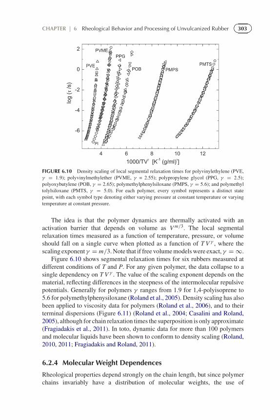
FIGURE 6.10 Density scaling of local segmental relaxation times for polyvinylethylene (PVE,γ = 1.9); polyvinylmethylether (PVME, γ = 2.55); polypropylene glycol (PPG, γ = 2.5);polyoxybutylene (POB, γ = 2.65); polymethylphenylsiloxane (PMPS, γ = 5.6); and polymethyltolylsiloxane (PMTS, γ = 5.0). For each polymer, every symbol represents a distinct statepoint, with each symbol type denoting either varying pressure at constant temperature or varyingtemperature at constant pressure.
The idea is that the polymer dynamics are thermally activated with anactivation barrier that depends on volume as V m/3. The local segmentalrelaxation times measured as a function of temperature, pressure, or volumeshould fall on a single curve when plotted as a function of T V γ , where thescaling exponent γ = m/3. Note that if free volume models were exact, γ = ∞.
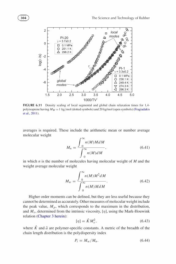
Figure 6.10 shows segmental relaxation times for six rubbers measured atdifferent conditions of T and P. For any given polymer, the data collapse to asingle dependency on T V γ . The value of the scaling exponent depends on thematerial, reflecting differences in the steepness of the intermolecular repulsivepotentials. Generally for polymers γ ranges from 1.9 for 1,4-polyisoprene to5.6 for polymethylphenysiloxane (Roland et al., 2005). Density scaling has alsobeen applied to viscosity data for polymers (Roland et al., 2006), and to theirterminal dispersions (Figure 6.11) (Roland et al., 2004; Casalini and Roland,2005), although for chain relaxation times the superposition is only approximate(Fragiadakis et al., 2011). In toto, dynamic data for more than 100 polymersand molecular liquids have been shown to conform to density scaling (Roland,2010, 2011; Fragiadakis and Roland, 2011).
6.2.4 Molecular Weight Dependences
Rheological properties depend strongly on the chain length, but since polymerchains invariably have a distribution of molecular weights, the use of
304 The Science and Technology of Rubber
FIGURE 6.11 Density scaling of local segmental and global chain relaxation times for 1,4-polyisoprene having MW =1 kg/mol (dotted symbols) and 20 kg/mol (open symbols) (Fragiadakiset al., 2011).
averages is required. These include the arithmetic mean or number averagemolecular weight
Mn =
∫ ∞
0n(M)Md M
∫ ∞
0n(M)d M
, (6.41)
in which n is the number of molecules having molecular weight of M and theweight average molecular weight
Mw =
∫ ∞
0n(M)M2d M
∫ ∞
0n(M)Md M
. (6.42)
Higher order moments can be defined, but they are less useful because theycannot be determined as accurately. Other measures of molecular weight includethe peak value, Mp, which corresponds to the maximum in the distribution,and Mv , determined from the intrinsic viscosity, [η], using the Mark-Houwinkrelation (Chapter 3 herein):
[η] = K Mav , (6.43)
where K and a are polymer-specific constants. A metric of the breadth of thechain length distribution is the polydispersity index
Pi = Mw/Mn . (6.44)
305CHAPTER | 6 Rheological Behavior and Processing of Unvulcanized Rubber
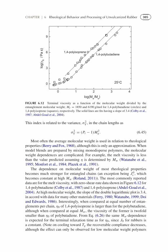
FIGURE 6.12 Terminal viscosity as a function of the molecular weight divided by theentanglement molecular weight; Me = 1850 and 6190 g/mol for 1,4-polybutadiene (circles) and1,4-polyisoprene (squares), respectively. The solid lines are fits having a slope of 3.4 (Colby et al.,1987; Abdel-Goad et al., 2004).
This index is related to the variance, σ 2V , in the chain lengths as
σ 2V = (Pi − 1)M2
n . (6.45)
Most often the average molecular weight is used in relation to rheologicalproperties (Berry and Fox, 1968), although this is only an approximation. Whenmodel blends are prepared by mixing monodisperse polymers, the molecularweight dependences are complicated. For example, the melt viscosity is lessthan the value predicted assuming η is determined by Mw (Watanabe et al.,1995; Monfort et al., 1984; Plazek et al., 1991).
The dependence on molecular weight of most rheological propertiesbecomes much stronger for entangled chains (an exception being J 0
s , whichbecomes constant at high Mw (Roland, 2011)). The most commonly reporteddata are for the melt viscosity, with zero-shear-rate data shown in Figure 6.12 for1,4-polybutadiene (Colby et al., 1987) and 1,4-polyisoprene (Abdel-Goad et al.,2004). At high molecular weight, the slope of the double logarithmic plot is 3.4,in accord with data for many other materials (Ferry, 1980; Watanabe, 1999; Doiand Edwards, 1986). Interestingly, when compared at equal number of entan-glements per chain, η0 of 1,4-polyisoprene is larger than for the polybutadiene,although when compared at equal Mw, the viscosity of the former is twofoldsmaller than η0 of polybutadiene. From Eq. (6.26) the same Mw-dependenceis expected for the terminal relaxation time as for η0, since J0 for rubbers isa constant. (Note on cooling toward Tg the recoverable compliance decreases,although the effect can only be observed for low molecular weight polymers
306 The Science and Technology of Rubber
(Roland et al., 2004; Ngai et al., 1995; Santangelo and Roland, 2001).) Thediffusion constant of rubbers has a quadratic or somewhat stronger molecularweight dependence (Lodge, 1999; Wang, 2003).
Various characteristic molecular weights can be defined from the molecularweight dependences of the rheological properties, including the molecularweight between entanglements, Me, determined from the plateau modulus
Me = ρRT
G N. (6.46)
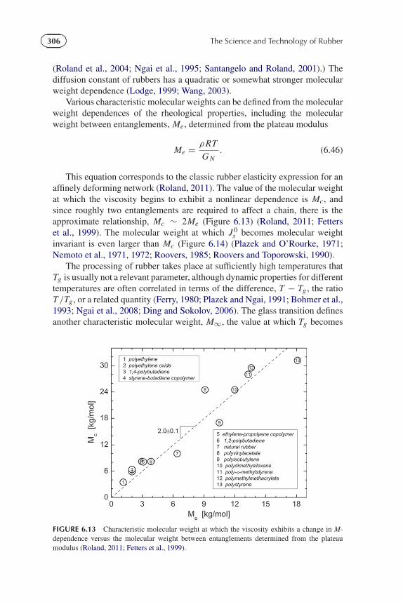
This equation corresponds to the classic rubber elasticity expression for anaffinely deforming network (Roland, 2011). The value of the molecular weightat which the viscosity begins to exhibit a nonlinear dependence is Mc, andsince roughly two entanglements are required to affect a chain, there is theapproximate relationship, Mc ∼ 2Me (Figure 6.13) (Roland, 2011; Fetterset al., 1999). The molecular weight at which J 0
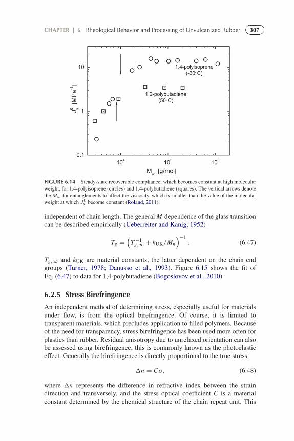
s becomes molecular weightinvariant is even larger than Mc (Figure 6.14) (Plazek and O’Rourke, 1971;Nemoto et al., 1971, 1972; Roovers, 1985; Roovers and Toporowski, 1990).
The processing of rubber takes place at sufficiently high temperatures thatTg is usually not a relevant parameter, although dynamic properties for differenttemperatures are often correlated in terms of the difference, T − Tg , the ratioT /Tg , or a related quantity (Ferry, 1980; Plazek and Ngai, 1991; Bohmer et al.,1993; Ngai et al., 2008; Ding and Sokolov, 2006). The glass transition definesanother characteristic molecular weight, M∞, the value at which Tg becomes
FIGURE 6.13 Characteristic molecular weight at which the viscosity exhibits a change in M-dependence versus the molecular weight between entanglements determined from the plateaumodulus (Roland, 2011; Fetters et al., 1999).
307CHAPTER | 6 Rheological Behavior and Processing of Unvulcanized Rubber
FIGURE 6.14 Steady-state recoverable compliance, which becomes constant at high molecularweight, for 1,4-polyisoprene (circles) and 1,4-polybutadiene (squares). The vertical arrows denotethe Mw for entanglements to affect the viscosity, which is smaller than the value of the molecularweight at which J 0
s become constant (Roland, 2011).
independent of chain length. The general M-dependence of the glass transitioncan be described empirically (Ueberreiter and Kanig, 1952)
Tg =(
T −1g,∞ + kUK/Mn
)−1. (6.47)
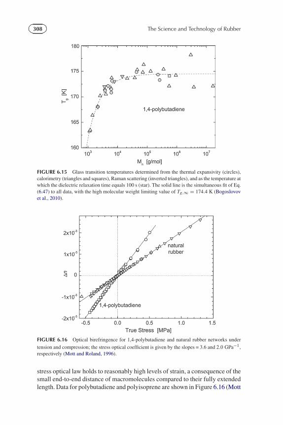
Tg,∞ and kUK are material constants, the latter dependent on the chain endgroups (Turner, 1978; Danusso et al., 1993). Figure 6.15 shows the fit ofEq. (6.47) to data for 1,4-polybutadiene (Bogoslovov et al., 2010).
6.2.5 Stress Birefringence
An independent method of determining stress, especially useful for materialsunder flow, is from the optical birefringence. Of course, it is limited totransparent materials, which precludes application to filled polymers. Becauseof the need for transparency, stress birefringence has been used more often forplastics than rubber. Residual anisotropy due to unrelaxed orientation can alsobe assessed using birefringence; this is commonly known as the photoelasticeffect. Generally the birefringence is directly proportional to the true stress
�n = Cσ, (6.48)
where �n represents the difference in refractive index between the straindirection and transversely, and the stress optical coefficient C is a materialconstant determined by the chemical structure of the chain repeat unit. This
308 The Science and Technology of Rubber
FIGURE 6.15 Glass transition temperatures determined from the thermal expansivity (circles),calorimetry (triangles and squares), Raman scattering (inverted triangles), and as the temperature atwhich the dielectric relaxation time equals 100 s (star). The solid line is the simultaneous fit of Eq.(6.47) to all data, with the high molecular weight limiting value of Tg,∞ = 174.4 K (Bogoslovovet al., 2010).
FIGURE 6.16 Optical birefringence for 1,4-polybutadiene and natural rubber networks under
tension and compression; the stress optical coefficient is given by the slopes = 3.6 and 2.0 GPa−1,respectively (Mott and Roland, 1996).
stress optical law holds to reasonably high levels of strain, a consequence of thesmall end-to-end distance of macromolecules compared to their fully extendedlength. Data for polybutadiene and polyisoprene are shown in Figure 6.16 (Mott
309CHAPTER | 6 Rheological Behavior and Processing of Unvulcanized Rubber
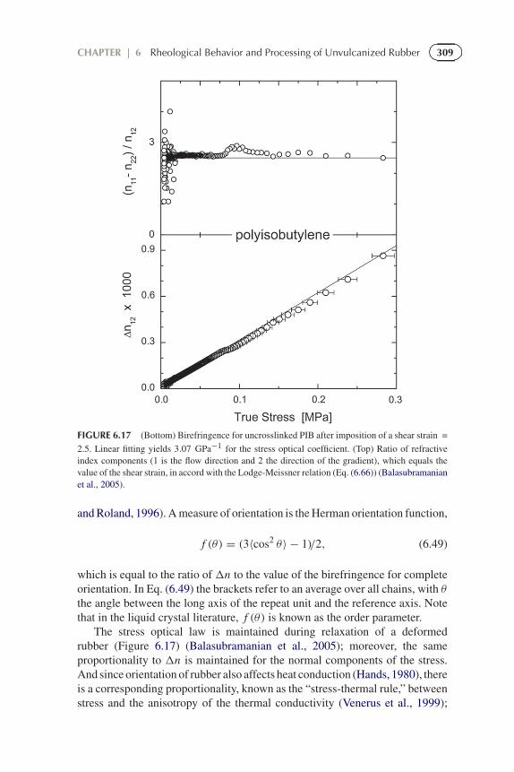
FIGURE 6.17 (Bottom) Birefringence for uncrosslinked PIB after imposition of a shear strain =
2.5. Linear fitting yields 3.07 GPa−1 for the stress optical coefficient. (Top) Ratio of refractiveindex components (1 is the flow direction and 2 the direction of the gradient), which equals thevalue of the shear strain, in accord with the Lodge-Meissner relation (Eq. (6.66)) (Balasubramanianet al., 2005).
and Roland, 1996). A measure of orientation is the Herman orientation function,
f (θ) = (3〈cos2 θ〉 − 1)/2, (6.49)
which is equal to the ratio of�n to the value of the birefringence for completeorientation. In Eq. (6.49) the brackets refer to an average over all chains, with θthe angle between the long axis of the repeat unit and the reference axis. Notethat in the liquid crystal literature, f (θ) is known as the order parameter.
The stress optical law is maintained during relaxation of a deformedrubber (Figure 6.17) (Balasubramanian et al., 2005); moreover, the sameproportionality to �n is maintained for the normal components of the stress.And since orientation of rubber also affects heat conduction (Hands, 1980), thereis a corresponding proportionality, known as the “stress-thermal rule,” betweenstress and the anisotropy of the thermal conductivity (Venerus et al., 1999);
310 The Science and Technology of Rubber
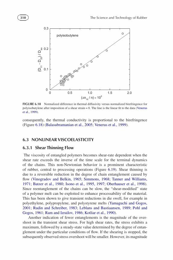
FIGURE 6.18 Normalized difference in thermal diffusivity versus normalized birefringence forpolyisobutylene after imposition of a shear strain = 8. The line is the linear fit to the data (Veneruset al., 1999).
consequently, the thermal conductivity is proportional to the birefringence(Figure 6.18) (Balasubramanian et al., 2005; Venerus et al., 1999).
6.3 NONLINEAR VISCOELASTICITY
6.3.1 Shear Thinning Flow
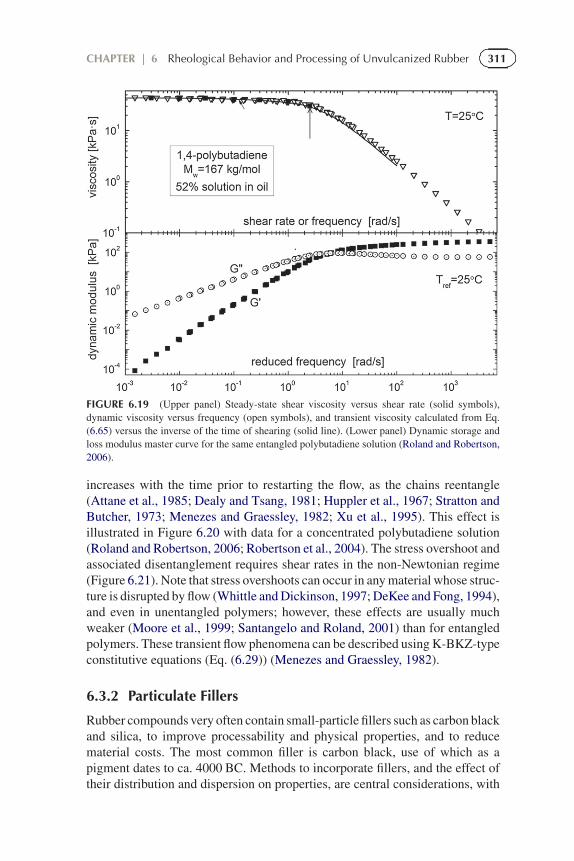
The viscosity of entangled polymers becomes shear-rate dependent when theshear rate exceeds the inverse of the time scale for the terminal dynamicsof the chains. This non-Newtonian behavior is a prominent characteristicof rubber, central to processing operations (Figure 6.19). Shear thinning isdue to a reversible reduction in the degree of chain entanglement caused byflow (Vinogradov and Belkin, 1965; Simmons, 1968; Tanner and Williams,1971; Batzer et al., 1980; Isono et al., 1995, 1997; Oberhauser et al., 1998).Since reentanglement of the chains can be slow, the “shear-modified” stateof a polymer melt can be exploited to enhance processability of the material.This has been shown to give transient reductions in die swell, for example inpolyethylene, polypropylene, and polystyrene melts (Yamaguchi and Gogos,2001; Rudin and Schreiber, 1983; Leblans and Bastiaansen, 1989; Pohl andGogos, 1961; Ram and Izrailov, 1986; Kotliar et al., 1990).
Another indication of fewer entanglements is the magnitude of the over-shoot in the transient shear stress. For high shear rates, the stress exhibits amaximum, followed by a steady-state value determined by the degree of entan-glement under the particular conditions of flow. If the shearing is stopped, thesubsequently observed stress overshoot will be smaller. However, its magnitude
311CHAPTER | 6 Rheological Behavior and Processing of Unvulcanized Rubber
FIGURE 6.19 (Upper panel) Steady-state shear viscosity versus shear rate (solid symbols),dynamic viscosity versus frequency (open symbols), and transient viscosity calculated from Eq.(6.65) versus the inverse of the time of shearing (solid line). (Lower panel) Dynamic storage andloss modulus master curve for the same entangled polybutadiene solution (Roland and Robertson,2006).
increases with the time prior to restarting the flow, as the chains reentangle(Attane et al., 1985; Dealy and Tsang, 1981; Huppler et al., 1967; Stratton andButcher, 1973; Menezes and Graessley, 1982; Xu et al., 1995). This effect isillustrated in Figure 6.20 with data for a concentrated polybutadiene solution(Roland and Robertson, 2006; Robertson et al., 2004). The stress overshoot andassociated disentanglement requires shear rates in the non-Newtonian regime(Figure 6.21). Note that stress overshoots can occur in any material whose struc-ture is disrupted by flow (Whittle and Dickinson, 1997; DeKee and Fong, 1994),and even in unentangled polymers; however, these effects are usually muchweaker (Moore et al., 1999; Santangelo and Roland, 2001) than for entangledpolymers. These transient flow phenomena can be described using K-BKZ-typeconstitutive equations (Eq. (6.29)) (Menezes and Graessley, 1982).
6.3.2 Particulate Fillers
Rubber compounds very often contain small-particle fillers such as carbon blackand silica, to improve processability and physical properties, and to reducematerial costs. The most common filler is carbon black, use of which as apigment dates to ca. 4000 BC. Methods to incorporate fillers, and the effect oftheir distribution and dispersion on properties, are central considerations, with
312 The Science and Technology of Rubber
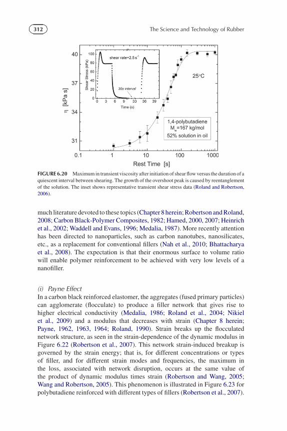
FIGURE 6.20 Maximum in transient viscosity after initiation of shear flow versus the duration of aquiescent interval between shearing. The growth of the overshoot peak is caused by reentanglementof the solution. The inset shows representative transient shear stress data (Roland and Robertson,2006).
much literature devoted to these topics (Chapter 8 herein; Robertson and Roland,2008; Carbon Black-Polymer Composites, 1982; Hamed, 2000, 2007; Heinrichet al., 2002; Waddell and Evans, 1996; Medalia, 1987). More recently attentionhas been directed to nanoparticles, such as carbon nanotubes, nanosilicates,etc., as a replacement for conventional fillers (Nah et al., 2010; Bhattacharyaet al., 2008). The expectation is that their enormous surface to volume ratiowill enable polymer reinforcement to be achieved with very low levels of ananofiller.
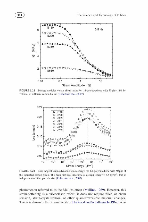
(i) Payne EffectIn a carbon black reinforced elastomer, the aggregates (fused primary particles)can agglomerate (flocculate) to produce a filler network that gives rise tohigher electrical conductivity (Medalia, 1986; Roland et al., 2004; Nikielet al., 2009) and a modulus that decreases with strain (Chapter 8 herein;Payne, 1962, 1963, 1964; Roland, 1990). Strain breaks up the flocculatednetwork structure, as seen in the strain-dependence of the dynamic modulus inFigure 6.22 (Robertson et al., 2007). This network strain-induced breakup isgoverned by the strain energy; that is, for different concentrations or typesof filler, and for different strain modes and frequencies, the maximum inthe loss, associated with network disruption, occurs at the same value ofthe product of dynamic modulus times strain (Robertson and Wang, 2005;Wang and Robertson, 2005). This phenomenon is illustrated in Figure 6.23 forpolybutadiene reinforced with different types of fillers (Robertson et al., 2007).
313CHAPTER | 6 Rheological Behavior and Processing of Unvulcanized Rubber
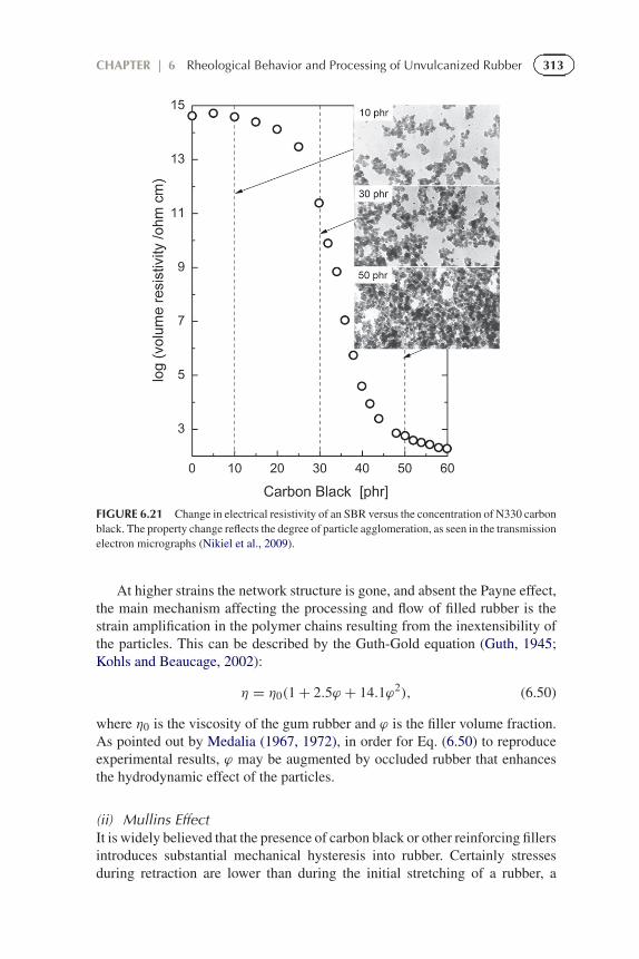
FIGURE 6.21 Change in electrical resistivity of an SBR versus the concentration of N330 carbonblack. The property change reflects the degree of particle agglomeration, as seen in the transmissionelectron micrographs (Nikiel et al., 2009).
At higher strains the network structure is gone, and absent the Payne effect,the main mechanism affecting the processing and flow of filled rubber is thestrain amplification in the polymer chains resulting from the inextensibility ofthe particles. This can be described by the Guth-Gold equation (Guth, 1945;Kohls and Beaucage, 2002):
η = η0(1 + 2.5ϕ + 14.1ϕ2), (6.50)
where η0 is the viscosity of the gum rubber and ϕ is the filler volume fraction.As pointed out by Medalia (1967, 1972), in order for Eq. (6.50) to reproduceexperimental results, ϕ may be augmented by occluded rubber that enhancesthe hydrodynamic effect of the particles.
(ii) Mullins EffectIt is widely believed that the presence of carbon black or other reinforcing fillersintroduces substantial mechanical hysteresis into rubber. Certainly stressesduring retraction are lower than during the initial stretching of a rubber, a
314 The Science and Technology of Rubber
FIGURE 6.22 Storage modulus versus shear strain for 1,4-polybutadiene with 50 phr (18% byvolume) of different carbon blacks (Robertson et al., 2007).
FIGURE 6.23 Loss tangent versus dynamic strain energy for 1,4-polybutadiene with 50 phr of
the indicated carbon black. The peak maxima superpose at a strain energy = 3.5 kJ/m3, that isindependent of filler particle size (Robertson et al., 2007).
phenomenon referred to as the Mullins effect (Mullins, 1969). However, thisstrain-softening is a viscoelastic effect; it does not require filler, or chainscission, strain-crystallization, or other quasi-irreversible material changes.This was shown in the original work of Harwood and Schallamach (1967), who
315CHAPTER | 6 Rheological Behavior and Processing of Unvulcanized Rubber
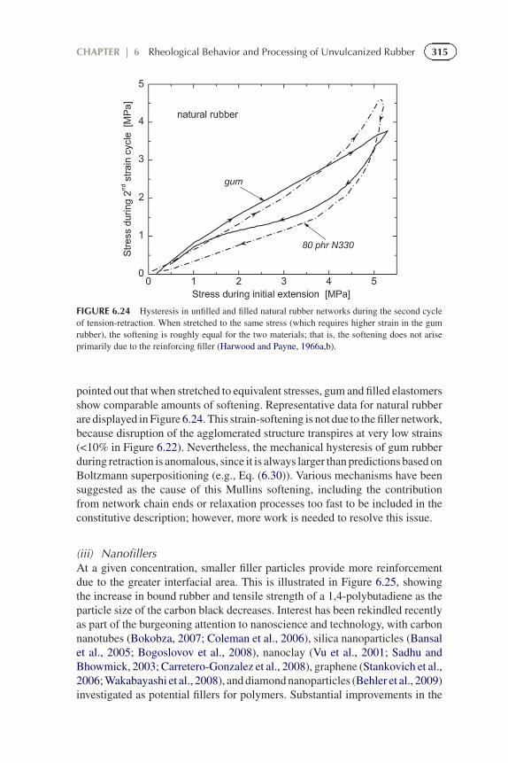
FIGURE 6.24 Hysteresis in unfilled and filled natural rubber networks during the second cycleof tension-retraction. When stretched to the same stress (which requires higher strain in the gumrubber), the softening is roughly equal for the two materials; that is, the softening does not ariseprimarily due to the reinforcing filler (Harwood and Payne, 1966a,b).
pointed out that when stretched to equivalent stresses, gum and filled elastomersshow comparable amounts of softening. Representative data for natural rubberare displayed in Figure 6.24. This strain-softening is not due to the filler network,because disruption of the agglomerated structure transpires at very low strains(<10% in Figure 6.22). Nevertheless, the mechanical hysteresis of gum rubberduring retraction is anomalous, since it is always larger than predictions based onBoltzmann superpositioning (e.g., Eq. (6.30)). Various mechanisms have beensuggested as the cause of this Mullins softening, including the contributionfrom network chain ends or relaxation processes too fast to be included in theconstitutive description; however, more work is needed to resolve this issue.
(iii) NanofillersAt a given concentration, smaller filler particles provide more reinforcementdue to the greater interfacial area. This is illustrated in Figure 6.25, showingthe increase in bound rubber and tensile strength of a 1,4-polybutadiene as theparticle size of the carbon black decreases. Interest has been rekindled recentlyas part of the burgeoning attention to nanoscience and technology, with carbonnanotubes (Bokobza, 2007; Coleman et al., 2006), silica nanoparticles (Bansalet al., 2005; Bogoslovov et al., 2008), nanoclay (Vu et al., 2001; Sadhu andBhowmick, 2003; Carretero-Gonzalez et al., 2008), graphene (Stankovich et al.,2006; Wakabayashi et al., 2008), and diamond nanoparticles (Behler et al., 2009)investigated as potential fillers for polymers. Substantial improvements in the
316 The Science and Technology of Rubber
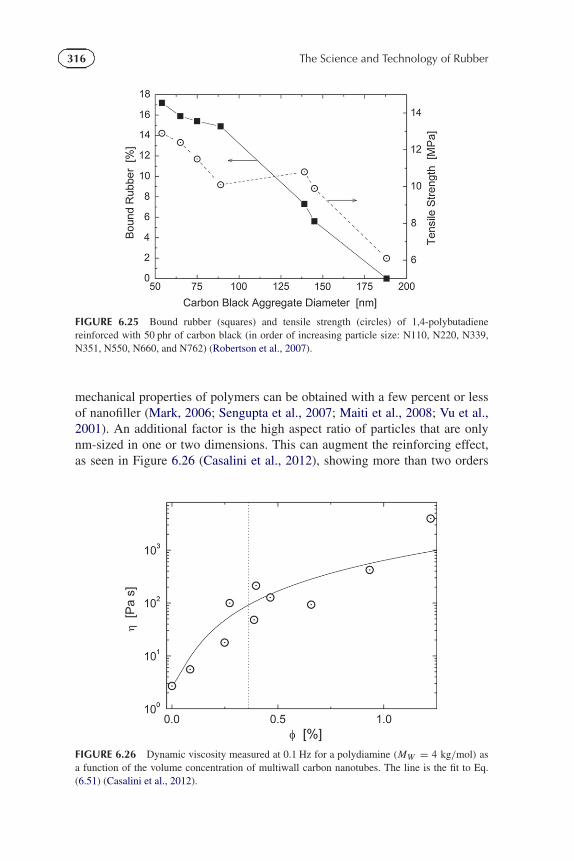
FIGURE 6.25 Bound rubber (squares) and tensile strength (circles) of 1,4-polybutadienereinforced with 50 phr of carbon black (in order of increasing particle size: N110, N220, N339,N351, N550, N660, and N762) (Robertson et al., 2007).
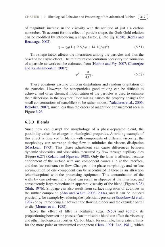
mechanical properties of polymers can be obtained with a few percent or lessof nanofiller (Mark, 2006; Sengupta et al., 2007; Maiti et al., 2008; Vu et al.,2001). An additional factor is the high aspect ratio of particles that are onlynm-sized in one or two dimensions. This can augment the reinforcing effect,as seen in Figure 6.26 (Casalini et al., 2012), showing more than two orders
FIGURE 6.26 Dynamic viscosity measured at 0.1 Hz for a polydiamine (MW = 4 kg/mol) asa function of the volume concentration of multiwall carbon nanotubes. The line is the fit to Eq.(6.51) (Casalini et al., 2012).
317CHAPTER | 6 Rheological Behavior and Processing of Unvulcanized Rubber
of magnitude increase in the viscosity with the addition of just 1% carbonnanotubes. To account for this effect of particle shape, the Guth-Gold relationcan be modified by introducing a shape factor, f, into Eq. (6.50) (Kohls andBeaucage, 2002):
η = η0(1 + 2.5 f ϕ + 14.1( f ϕ)2). (6.51)
This shape factor affects the interaction among the particles and thus theonset of the Payne effect. The minimum concentration necessary for formationof a particle network can be estimated from (Hobbie and Fry, 2007; Chatterjeeand Krishnamoortim, 2007):
ϕ∗ = π
4 f 2 . (6.52)
These equations assume uniform distribution and random orientation ofthe particles. However, for nanoparticles good mixing can be difficult toachieve, and often chemical modification of the particles is used to enhancetheir dispersion in the polymer. Poor mixing causes the property changes forsmall concentrations of nanofillers to be rather modest (Valadares et al., 2006;Bokobza, 2007), much less than the orders of magnitude enhancement seen inFigure 6.26.
6.3.3 Blends
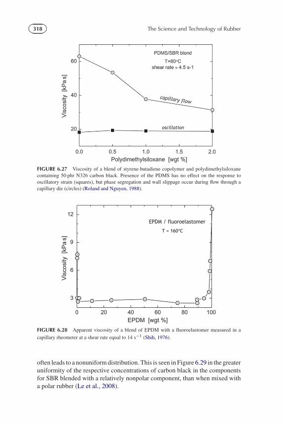
Since flow can disrupt the morphology of a phase-separated blend, thepossibility exists for changes in rheological properties. A striking example ofthis effect is observed in blends with components of different viscosity; themorphology can rearrange during flow to minimize the viscous dissipation(MacLean, 1973). This phase adjustment can cause differences betweendynamic viscosities and viscosities measured by flow through capillary dies(Figure 6.27) (Roland and Nguyen, 1988). Only the latter is affected becauseenrichment of the surface with one component causes slip at the interface,and thus less resistance to flow. Changes in the phase morphology and surfaceaccumulation of one component can be accentuated if there is an attraction(chemisorption) with the processing equipment. This contamination of thewalls by one polymer in a blend can result in slippage at the interface, andconsequently large reductions in apparent viscosity of the blend (Figure 6.28)(Shih, 1976). Slippage can also result from surface migration of additives inthe rubber compound (Ahn and White, 2003, 2004), and it can be inducedphysically, for example by reducing the hydrostatic pressure (Brzoskowski et al.,1987) or by introducing air between the flowing rubber and the extruder barrelor die (Montes et al., 1988).
Since the effect of filler is nonlinear (Eqs. (6.50) and (6.51)), itsproportioning between the phases of an immiscible blend can affect the viscosityand other rheological properties. Carbon black, for example, has greater affinityfor the more polar or unsaturated component (Hess, 1991; Lee, 1981), which
318 The Science and Technology of Rubber
FIGURE 6.27 Viscosity of a blend of styrene-butadiene copolymer and polydimethylsiloxanecontaining 50 phr N326 carbon black. Presence of the PDMS has no effect on the response tooscillatory strain (squares), but phase segregation and wall slippage occur during flow through acapillary die (circles) (Roland and Nguyen, 1988).
FIGURE 6.28 Apparent viscosity of a blend of EPDM with a fluoroelastomer measured in a
capillary rheometer at a shear rate equal to 14 s−1 (Shih, 1976).
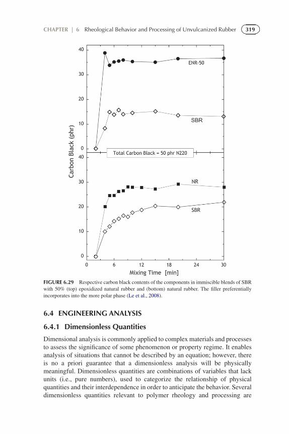
often leads to a nonuniform distribution. This is seen in Figure 6.29 in the greateruniformity of the respective concentrations of carbon black in the componentsfor SBR blended with a relatively nonpolar component, than when mixed witha polar rubber (Le et al., 2008).
319CHAPTER | 6 Rheological Behavior and Processing of Unvulcanized Rubber
FIGURE 6.29 Respective carbon black contents of the components in immiscible blends of SBRwith 50% (top) epoxidized natural rubber and (bottom) natural rubber. The filler preferentiallyincorporates into the more polar phase (Le et al., 2008).
6.4 ENGINEERING ANALYSIS
6.4.1 Dimensionless Quantities
Dimensional analysis is commonly applied to complex materials and processesto assess the significance of some phenomenon or property regime. It enablesanalysis of situations that cannot be described by an equation; however, thereis no a priori guarantee that a dimensionless analysis will be physicallymeaningful. Dimensionless quantities are combinations of variables that lackunits (i.e., pure numbers), used to categorize the relationship of physicalquantities and their interdependence in order to anticipate the behavior. Severaldimensionless quantities relevant to polymer rheology and processing are
320 The Science and Technology of Rubber
defined in the following. Although these are all ratios, this is not a requirementof dimensionless quantities; they can be characteristic numbers (e.g., quantumnumbers) or represent a count (such as a partition function).
(i) Reynolds NumberA very common quantity, this is the ratio of the inertial to viscous forces (Rott,1990):
Re ≡ ρvL
η, (6.53)
where ρ is the mass density, v is the velocity, and L is a characteristic dimension.For extensional and shear flows, L represents the dimension parallel andperpendicular, respectively, to the flow. Re can identify the laminar to turbulentflow transition for different fluids and different flow rates, independentlyof the geometry. For example, for flow in a circular pipe, L is the insidediameter, and the transition from laminar to turbulent flow occurs in the range2300 < Re < 4000. A variation on Re is the Blake Number (Blake, 1922),which applies to porous media, such as beds of solids.
(ii) Deborah NumberThe Deborah number is the ratio of the relaxation time of the material to theexperimental timescale:
De ≡ γ τ. (6.54)
A larger Deborah number implies a more elastic response. The term, whichcomes from the biblical quote in Section 6.1.1, was coined by Reiner (1964).
(iii) Weissenberg NumberDefined as the ratio of the material relaxation time to the processing time duringflow, Wi characterizes the amount of molecular orientation induced by the flow.For simple shear flow, Wi is given by the product of τ times the shear rate.Related to the Deborah number, Wi is used for constant straining, whereas Dedescribes deformations with a varying strain history.
(iv) Capillary NumberThis quantity is the ratio of the viscous force to the surface tension across aninterface,
Ca ≡ ηv
ϒ, (6.55)
where ϒ is the surface tension. Relevant to extensional flow from orifices anddomain formation during mixing of immiscible liquids, values of Ca larger thanunity imply stretching of dispersed particles or droplets, which is a necessary
321CHAPTER | 6 Rheological Behavior and Processing of Unvulcanized Rubber
condition for their dispersion. The ratio of the Deborah and capillary numbers,
De
Ca= τϒ
ηL, (6.56)
the “elastocapillary number” (Hsu and Leal, 2009), is a measure of thedeformation of dispersed phases that is independent of the strain rate. L inEq. (6.56) is related to the droplet size.
(v) Weber NumberAnalogous to the capillary number, We is the ratio of the inertial force to thesurface tension across an interface,
W e ≡ ρv2 L
ϒ. (6.57)
(vi) Brinkman NumberThis number, used in polymer processing, describes the heat flow between theflowing material and the vessel containing it (e.g., the rotor and walls of anextruder). It is defined as
Br ≡ ηv2
κ�T, (6.58)
in which κ is the thermal conductivity of the material and �T its temperaturedifference with the vessel. A large value of Br(>1) indicates significant viscousheating.
(vii) Bingham NumberUsed to characterize a polymer that flows when the stress reaches a characteristiclevel (Bingham, 1916), this number is the ratio of the yield stress, σY , to theviscous stress,
Bn ≡ σY L
ηv. (6.59)
(viii) Elasticity NumberThe ratio of the elastic forces to the inertial forces,
El = τη
ρL2 . (6.60)
and equal to the Weissenberg number divided by the Reynolds numbers, Elcharacterizes the effect of elasticity on the flow. For a polymer solution Eldepends only on the material properties, except for the size of the flow device.
322 The Science and Technology of Rubber
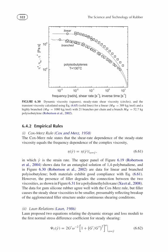
FIGURE 6.30 Dynamic viscosity (squares), steady-state shear viscosity (circles), and thetransient viscosity calculated using Eq. (6.65) (solid lines) for a linear (MW = 389 kg/mol) and ahighly branched (MW = 1080 kg/mol) with 21 branches per chain and a branch MW = 52.7 kgpolyisobutylene (Robertson et al., 2002).
6.4.2 Empirical Rules
(i) Cox-Merz Rule (Cox and Merz, 1958)The Cox-Merz rule states that the shear-rate dependence of the steady-stateviscosity equals the frequency dependence of the complex viscosity,
η(γ ) = η(γ )|ω=γ , (6.61)
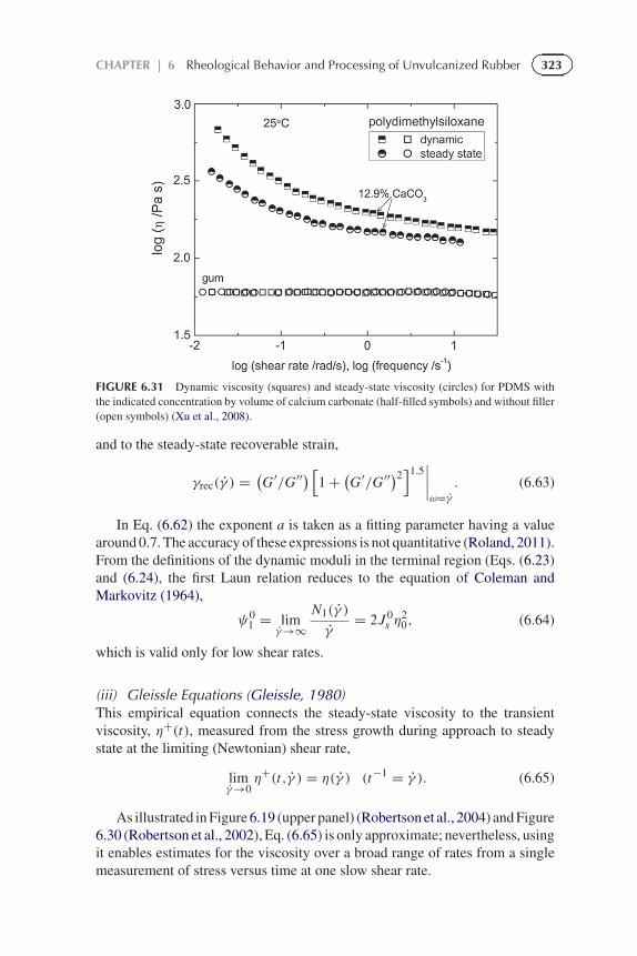
in which γ is the strain rate. The upper panel of Figure 6.19 (Robertsonet al., 2004) shows data for an entangled solution of 1,4-polybutadiene, andin Figure 6.30 (Robertson et al., 2002) are data for linear and branchedpolyisobutylene; both materials exhibit good compliance with Eq. (6.61).However, the presence of filler degrades the connection between the twoviscosities, as shown in Figure 6.31 for a polydimethylsiloxane (Xu et al., 2008).The data for gum silicone rubber agree well with the Cox-Merz rule, but fillercauses the steady shear viscosities to be smaller, presumably reflecting breakupof the agglomerated filler structure under continuous shearing conditions.
(ii) Laun Relations (Laun, 1986)Laun proposed two equations relating the dynamic storage and loss moduli tothe first normal stress difference coefficient for steady shearing:
1(γ ) = 2G ′ω−2[1 + (
G ′/G ′′)2]a∣∣∣ω=γ (6.62)
323CHAPTER | 6 Rheological Behavior and Processing of Unvulcanized Rubber
FIGURE 6.31 Dynamic viscosity (squares) and steady-state viscosity (circles) for PDMS withthe indicated concentration by volume of calcium carbonate (half-filled symbols) and without filler(open symbols) (Xu et al., 2008).
and to the steady-state recoverable strain,
γrec(γ ) = (G ′/G ′′) [1 + (
G ′/G ′′)2]1.5∣∣∣∣ω=γ
. (6.63)
In Eq. (6.62) the exponent a is taken as a fitting parameter having a valuearound 0.7. The accuracy of these expressions is not quantitative (Roland, 2011).From the definitions of the dynamic moduli in the terminal region (Eqs. (6.23)and (6.24), the first Laun relation reduces to the equation of Coleman andMarkovitz (1964),
ψ01 = lim
γ→∞N1(γ )
γ= 2J 0
s η20, (6.64)
which is valid only for low shear rates.
(iii) Gleissle Equations (Gleissle, 1980)This empirical equation connects the steady-state viscosity to the transientviscosity, η+(t), measured from the stress growth during approach to steadystate at the limiting (Newtonian) shear rate,
limγ→0
η+(t,γ ) = η(γ ) (t−1 = γ ). (6.65)
As illustrated in Figure 6.19 (upper panel) (Robertson et al., 2004) and Figure6.30 (Robertson et al., 2002), Eq. (6.65) is only approximate; nevertheless, usingit enables estimates for the viscosity over a broad range of rates from a singlemeasurement of stress versus time at one slow shear rate.
324 The Science and Technology of Rubber
(iv) Lodge-Meissner Rule (Lodge and Meissner, 1972)After imposition of a step strain, the ratio of the first normal stress difference,N1, to the shear stress is equal to the strain, or
N1(t) = ε2G(t) = εσ (t). (6.66)
This behavior is apparent in the top panel of Figure 6.17, showing thatthe birefringence perpendicular to the strain direction has the same time-dependence as the stress.
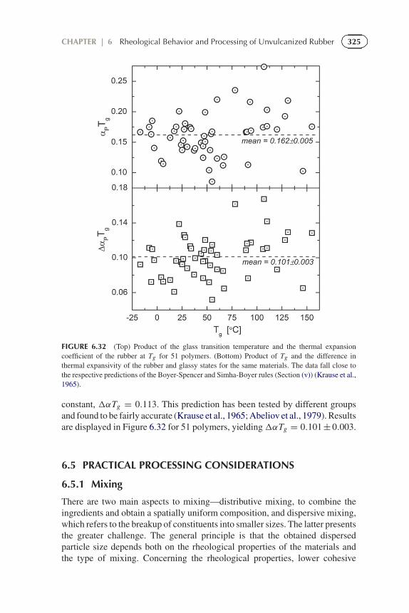
(v) Boyer-Spencer (Boyer and Spencer, 1944) and Simha-Boyer (Simhaand Boyer, 1962) Rules
From analysis of data for various polymers, two correlations have been reportedconcerning properties at the glass transition. The rationalization for both relieson a free volume description of the glass transition in polymers, which meansthe correlations are strictly empirical. The Boyer-Spencer rule (Boyer andSpencer, 1944) posits that the product of the glass transition temperature andthe thermal expansion coefficient at Tg is a universal constant, αP Tg = 0.113.An alternative analysis of Bondi (Van Krevelen, 1990) gives αP Tg = 0.116.The data in Figure 6.32 (Krause et al., 1965) show that this empirical rule isreasonably accurate, with a mean for 51 amorphous polymers yielding αP Tg =0.162 ± 0.005. This correlation is affirmed by the density scaling property (Eq.(6.40)), from which a relation between γ and the ratio of the isochoric andisobaric activation energies can be derived (Casalini and Roland, 2004a):
EV
EP= (1 + αP T γ )−1, (6.67)
where the isobaric activation energy (which is more properly called an activationenthalpy) has its usual definition,
EP (T ,P) = R∂ ln τ
∂T −1
∣∣∣∣P, (6.68)
and the activation energy at constant density is
EV (T ,V ) = R∂ ln τ
∂T −1
∣∣∣∣V. (6.69)
EV /EP can be calculated from segmental relaxation times for polymers androtational correlation times of molecular liquids, measured over a range ofthermodynamic conditions. Plots of the activation energy ratio versus γ canbe fit using a value of αP Tg = 0.18 ± 0.01 (Casalini and Roland, 2004b),consistent with the Boyer-Spencer rule.
According to the Simha-Boyer rule (Simha and Boyer, 1962), the product ofthe Tg times the change in thermal expansivity at Tg is a material-independent
325CHAPTER | 6 Rheological Behavior and Processing of Unvulcanized Rubber
FIGURE 6.32 (Top) Product of the glass transition temperature and the thermal expansioncoefficient of the rubber at Tg for 51 polymers. (Bottom) Product of Tg and the difference inthermal expansivity of the rubber and glassy states for the same materials. The data fall close tothe respective predictions of the Boyer-Spencer and Simha-Boyer rules (Section (v)) (Krause et al.,1965).
constant, �αTg = 0.113. This prediction has been tested by different groupsand found to be fairly accurate (Krause et al., 1965; Abeliov et al., 1979). Resultsare displayed in Figure 6.32 for 51 polymers, yielding�αTg = 0.101 ± 0.003.
6.5 PRACTICAL PROCESSING CONSIDERATIONS
6.5.1 Mixing
There are two main aspects to mixing—distributive mixing, to combine theingredients and obtain a spatially uniform composition, and dispersive mixing,which refers to the breakup of constituents into smaller sizes. The latter presentsthe greater challenge. The general principle is that the obtained dispersedparticle size depends both on the rheological properties of the materials andthe type of mixing. Concerning the rheological properties, lower cohesive
326 The Science and Technology of Rubber
strength of the dispersed component and a closer matching of its viscosity(assuming fluid particles) to that of the matrix leads to more effective dispersion(Rallison, 1984; Grace, 1982; Nelson et al., 1977). The type of mixing affectsthe dispersion process primarily because stretching flows are most effective atdispersion and rotational flows are completely ineffective. In order to sustainthe stresses and thereby fracture the particle, flow field vorticity should besuppressed, since reorientation of the particles or domains allows the stressesto successively counterbalance each other. Beyond this consideration, theobjective is to apply the highest stresses and strain rates, provided degradation(chain scission) is not an issue, and to ensure that all the material passes throughthe regions of the mixing vessel at which dispersion forces are greatest. Verygenerally, the strain rate tensor can be written as
� ≡ ∇v =
⎛⎜⎜⎜⎜⎜⎝
∂vx
∂x
∂vx
∂ y
∂vx
∂z∂vy
∂x
∂vy
∂ y
∂vy
∂z∂vz
∂x
∂vz
∂ y
∂vz
∂z
⎞⎟⎟⎟⎟⎟⎠. (6.70)
A metric for the strength of the flow field, ζ , can be introduced, whereζ = 1 for pure extensional flow and −1 for rotation (Fuller and Leal, 1981).The strength of the flow field is then given by the ratio of the stretching to the
vorticity, equal to1 + ζ
1 − ζ. For two-dimensional flow (Fuller and Leal, 1981),
� = γ
2
⎛⎜⎝
(1 + ζ ) (1 − ζ ) 0
(−1 + ζ ) (−1 − ζ ) 0
0 0 0
⎞⎟⎠ , (6.71)
where γ represents the local velocity gradient. An arbitrary flow field can beexpressed as the linear superposition of pure stretching and rotational flow,with shear flow corresponding to ζ = 0. Using their strength criteria, moredispersion will occur on the entrance to a capillary die, associated with ζ closeto unity, than for shearing flow through the die. The effect of slippage of thepolymer is to reduce the velocity gradient; thus (Fuller and Leal, 1981),
�eff = γ
2
⎛⎜⎝(1 − ξ)(1 + ζ ) (1 − ζ ) 0
(−1 + ζ ) −(1 − ξ)(−1 − ζ ) 0
0 0 0
⎞⎟⎠ , (6.72)
with ξ a measure of the slippage. The strength of the flow field is now given by(1 − ξ)(1 + ζ )
1 − ζ.
These considerations apply both to mixing of the components of a polymerblend and to dispersion of particulate fillers. For blends the obtained size of the
327CHAPTER | 6 Rheological Behavior and Processing of Unvulcanized Rubber
dispersed phase represents the competition between breakup of the particlesand their flow-induced coalescence (Roland and Bohm, 1984; Sirisinha et al.,2003; Chen et al., 2006; Peng et al., 2011). Similarly, the final degree of fillerdispersion depends not only on the breakup of the aggregates during mixing,but also on the extent of reagglomeration, which occurs, for example, duringcuring or thermal annealing (Bohm and Nguyen, 1995; Mihara et al., 2009;Schwartz et al., 2003). Chemical treatment of the filler surface is a commonmethod to suppress agglomeration, either with coupling agents that promoteinteraction with the polymer, or using shielding agents to decrease filler-fillerinteractions (Robertson et al., 2008; Ye et al., 2012; Lin et al., 2010).
6.5.2 Die Swell
When rubber is deformed during processing operations such as extrusion orcalendaring, its inherent elasticity will cause some subsequent recovery. Afundamental material constant characterizing this tendency is J 0
s , defined inEqs. (6.12) and (6.14). Elastic recovery is also reflected in die swell, D,defined as the ratio of the final and initial dimensions perpendicular to theflow. Die swell is governed by the normal force, although predictions of Dfor an arbitrary deformation are not possible. However, for steady-state flowthere are approximate relations between D and the first (primary) normal force(Tanner, 1970),
N1 = 2σ(2D6 − 2)1/2, (6.73)
and (Bagley and Duffey, 1970),
N1 = 2σ(2D4 − D−2). (6.74)
Substituting for the stress in Eq. (6.66), D can be related to the shear strain,or using Eq. (6.62) to the dynamic modulus. Results are shown in Figure 6.33(Müllner et al., 2008), comparing the die swell measured in a capillary rheometerto values calculated from dynamic measurements. The rough agreement withexperimentally measured die swell is satisfactory given the approximate natureof the derivation of Eqs. (6.73) or (6.74) (Tanner, 1970; Bagley and Duffey,1970).
As mentioned in Section 6.3.3, the affinity of filler for a rubber is expectedto be greater for more polar rubbers and those having a higher degree ofunsaturation, and this can result in a nonuniform distribution of the fillerbetween the phases of a blend (Hess, 1991; Lee, 1981; Le et al., 2008). Sinceactive fillers such as carbon black interact with the polymer chains, mainly viachemisorption, there is little migration between the phases. This means that anonuniform distribution can be obtained by design, through the sequence inwhich the materials are added to the mixing. Properties such as the elasticitydepend nonlinearly on the filler content, which means a rubber blend havinga nonuniform distribution can behave differently than one in which the filler
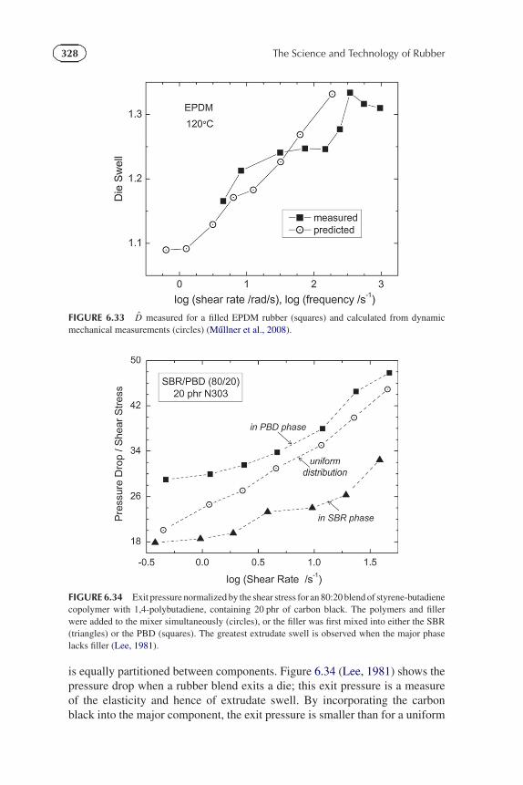
328 The Science and Technology of Rubber
FIGURE 6.33 D measured for a filled EPDM rubber (squares) and calculated from dynamicmechanical measurements (circles) (Mullner et al., 2008).
FIGURE 6.34 Exit pressure normalized by the shear stress for an 80:20 blend of styrene-butadienecopolymer with 1,4-polybutadiene, containing 20 phr of carbon black. The polymers and fillerwere added to the mixer simultaneously (circles), or the filler was first mixed into either the SBR(triangles) or the PBD (squares). The greatest extrudate swell is observed when the major phaselacks filler (Lee, 1981).
is equally partitioned between components. Figure 6.34 (Lee, 1981) shows thepressure drop when a rubber blend exits a die; this exit pressure is a measureof the elasticity and hence of extrudate swell. By incorporating the carbonblack into the major component, the exit pressure is smaller than for a uniform
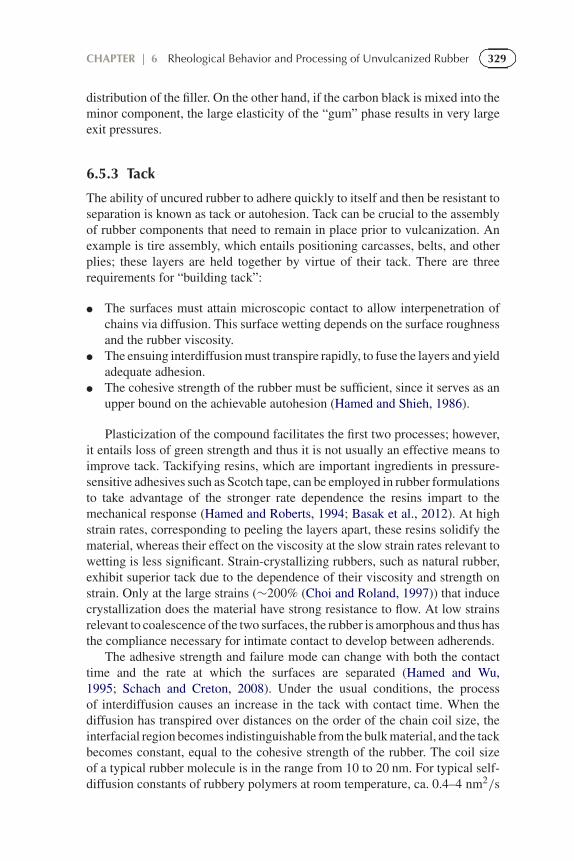
329CHAPTER | 6 Rheological Behavior and Processing of Unvulcanized Rubber
distribution of the filler. On the other hand, if the carbon black is mixed into theminor component, the large elasticity of the “gum” phase results in very largeexit pressures.
6.5.3 Tack
The ability of uncured rubber to adhere quickly to itself and then be resistant toseparation is known as tack or autohesion. Tack can be crucial to the assemblyof rubber components that need to remain in place prior to vulcanization. Anexample is tire assembly, which entails positioning carcasses, belts, and otherplies; these layers are held together by virtue of their tack. There are threerequirements for “building tack”:
● The surfaces must attain microscopic contact to allow interpenetration ofchains via diffusion. This surface wetting depends on the surface roughnessand the rubber viscosity.
● The ensuing interdiffusion must transpire rapidly, to fuse the layers and yieldadequate adhesion.
● The cohesive strength of the rubber must be sufficient, since it serves as anupper bound on the achievable autohesion (Hamed and Shieh, 1986).
Plasticization of the compound facilitates the first two processes; however,it entails loss of green strength and thus it is not usually an effective means toimprove tack. Tackifying resins, which are important ingredients in pressure-sensitive adhesives such as Scotch tape, can be employed in rubber formulationsto take advantage of the stronger rate dependence the resins impart to themechanical response (Hamed and Roberts, 1994; Basak et al., 2012). At highstrain rates, corresponding to peeling the layers apart, these resins solidify thematerial, whereas their effect on the viscosity at the slow strain rates relevant towetting is less significant. Strain-crystallizing rubbers, such as natural rubber,exhibit superior tack due to the dependence of their viscosity and strength onstrain. Only at the large strains (∼200% (Choi and Roland, 1997)) that inducecrystallization does the material have strong resistance to flow. At low strainsrelevant to coalescence of the two surfaces, the rubber is amorphous and thus hasthe compliance necessary for intimate contact to develop between adherends.
The adhesive strength and failure mode can change with both the contacttime and the rate at which the surfaces are separated (Hamed and Wu,1995; Schach and Creton, 2008). Under the usual conditions, the processof interdiffusion causes an increase in the tack with contact time. When thediffusion has transpired over distances on the order of the chain coil size, theinterfacial region becomes indistinguishable from the bulk material, and the tackbecomes constant, equal to the cohesive strength of the rubber. The coil sizeof a typical rubber molecule is in the range from 10 to 20 nm. For typical self-diffusion constants of rubbery polymers at room temperature, ca. 0.4–4 nm2/s
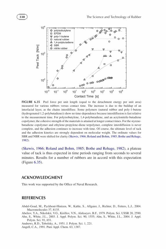
330 The Science and Technology of Rubber
FIGURE 6.35 Peel force per unit length (equal to the detachment energy per unit area)measured for various rubbers versus contact time. The increase is due to the buildup of aninterfacial layer, as the chains interdiffuse. Some polymers (natural rubber and poly-1-butene(hydrogenated 1,2-polybutadiene)) show no time-dependence because interdiffusion is fast relativeto the measurement time. For polyisobutylene, 1,4-polybutadiene, and an acrylonitrile-butadienecopolymer, the cohesive strength of the materials is attained at longer contact times. For the styrene-butadiene copolymer and ethylene-propylene-diene terpolymer, complete interdiffusion is nevercomplete, and the adhesion continues to increase with time. Of course, the ultimate level of tackand the adhesion kinetics are strongly dependent on molecular weight. The ordinate values forSBR and NBR were shifted for clarity (Skewis, 1966; Roland and Bohm, 1985; Bothe and Rehage,1982).
(Skewis, 1966; Roland and Bohm, 1985; Bothe and Rehage, 1982), a plateauvalue of tack is thus expected in time periods ranging from seconds to severalminutes. Results for a number of rubbers are in accord with this expectation(Figure 6.35).
ACKNOWLEDGMENT
This work was supported by the Office of Naval Research.
REFERENCES
Abdel-Goad, M., Pyckhout-Hintzen, W., Kahle, S., Allgaier, J., Richter, D., Fetters, L.J., 2004.Macromolecules 37, 8135.
Abeliov, Y.A., Nikolskii, V.G., Kirillov, V.N., Alekseyev, B.F., 1979. Polym. Sci. USSR 20, 2590.Ahn, S., White, J.L., 2003. J. Appl. Polym. Sci. 90, 1555; Ahn, S., White, J.L., 2004. J. Appl.
Polym. Sci. 91, 651.Andrews, R.D., Tobolsky, A., 1951. J. Polym. Sci. 1, 221.Angell, C.A., 1991. Pure Appl. Chem. 63, 1387.
331CHAPTER | 6 Rheological Behavior and Processing of Unvulcanized Rubber
Angell, C.A., Ngai, K.L., McKenna, G.B., McMillan, P.F., 2000. J. Appl. Phys. 88, 3113.Arruda, E., Wang, Y., Przbylo, P., 2001. Rubber Chem. Technol. 74, 560.Ashurst, W.T., Hoover, W.G., 1975. Phys. Rev. A 11, 658.Attane, P., Pierrard, J.M., Turrel, G., 1985. J. Non-Newton. Fluid Mech. 18, 295.Bagley, E.B., Duffey, H.J., 1970. Trans. Soc. Rheol. 14, 545.Bair, S., 2002. J. Eng. Tribol. 216, 1.Bair, S., Winer, W.O., 1980. J. Lubricat. Technol. 102, 229.Baird, D.G., Collias, D.I., 1998. Polymer Processing: Principles and Design. Wiley-Interscience.Balasubramanian, V., Bush, K., Smoukov, S., Venerus, D.C., Schieber, J.D., 2005. Macromolecules
38, 6210.Bansal, A., Yang, H.C., Li, C.Z., Cho, K.W., Benicewicz, B.C., Kumar, S.K., Schadler, L.S., 2005.
Nat. Mater. 4, 693.Bardik, V.Y., Sysoev, V.M., 1998. Low Temp. Phys. 24, 601.Basak, G.C., Bandyopadhyay, A., Bhowmick, A.K., 2012. J. Mater. Sci. 47, 3166.Batzer, H., Wagner, M.H., Meissner, J., 1980. Makromol. Chem. 181, 1533.Behler, K.D., Stravato, A., Mochalin, V., Korneva, G., Yushin, G., Gogotsi, Y., 2009. ACS Nano.
3, 363.Bergstrom, J.S., Boyce, M.C., 1998. J. Mech. Phys. Solids 46, 931.Bernstein, B., Kearsley, E.A., Zapas, L.J., 1963. Trans. Soc. Rheol. 7, 391.Bernstein, B., Kearsley, E.A., Zapas, L.J., 1964. J. Res. Natl. Bur. Stand., Sect. B 68, 103.Berry, G.C., 2003. Polymer Rheology: Principles, Techniques and Applications. In: Brady, J.R.F.
(Ed.), Desk Reference of Polymer Characterization and Analysis. American Chemical Society,New York, p. 574.
Berry, G.C., Fox, T.G., 1968. Adv. Polym. Sci. 5, 261.Bhattacharya, M., Maiti, M., Bhowmick, A.K., 2008. Rubber Chem. Technol. 81, 782.Bingham, E.C., 1916. US Bureau Stand. Bull. 13, 309.Blake, F.C., 1922. Trans. AIChE 14, 415.Boese, D., Momper, B., Meier, G., Kremer, F., Hagenah, I.U., Fischer, E.W., 1989. Macromolecules
22, 4416.Bogoslovov, R.B., Roland, C.M., Ellis, A.R., Randall, A.M., Robertson, C.G., 2008.
Macromolecules 41, 1289.Bogoslovov, R.B., Hogan, T.E., Roland, C.M., 2010. Macromolecules 43, 2904.Bohm, G.G.A., Nguyen, M.N., 1995. J. Appl. Polym. Sci. 55, 1041.Bohmer, R., Ngai, K.L., Angell, C.A., Plazek, D.J., 1993. J. Chem. Phys. 99, 4201.Bokobza, L., 2007. Polymer 48, 4907.Boltzmann, L., 1874. Sitzungsber. Kaiserl. Akad. Wiss. Wien 70, 275.Bothe, L., Rehage, G., 1982. Rubber Chem. Technol. 55, 1308.Boyer, R.F., Spencer, R.S., 1944. J. Appl. Phys. 15, 398.Brochard, F., De Gennes, P.G., 1977. Macromolecules 10, 1157.Brzoskowski, R., White, J.L., Szydlowski, W., Weissert, F.C., Nakajima, N., Min, K., 1987. Rubber
Chem. Technol. 60, 945.Carretero-Gonzalez, J., Retsos, H., Verdejo, R., Toki, S., Hsiao, B.S., Giannelis, E.P., Lopez-
Manchado, M.A., 2008. Macromolecules 41, 6763.Casalini, R., Roland, C.M., 2004a. Phys. Rev. E 69, 062501.Casalini, R., Roland, C.M., 2004b. Coll. Polym. Sci. 283, 107.Casalini, R., Roland, C.M., 2005. Macromolecules 38, 1779.Casalini, R., Bogoslovov, R., Qadri, S.B., Roland, C.M., 2012. Polymer 53, 1282.Chandler, D., Weeks, J.D., Andersen, H.C., 1983. Science 220, 787.Chang, I., Sillescu, H., 1997. J. Phys. Chem. B 101, 8794.Chang, W.V., Bloch, R., Tschoegl, N.W., 1976. Rheol. Acta 15, 367.Chapter 3 herein.Chapter 8 herein.Chatterjee, T., Krishnamoortim, R., 2007. Phys. Rev. E 75, 050403.Chen, X., Xi, J., Guo, B.H., 2006. J. Appl. Polym. Sci. 102, 3201.Choi, I.S., Roland, C.M., 1997. Rubber Chem. Technol. 70, 202.Cohen, M.H., Grest, G.S., 1979. Phys. Rev. B 20, 1077.Cohen, M.H., Grest, G.S., 1984. J. Non-Cryst. Solids 61–62, 749.Cohen, M.H., Turnbull, D., 1959. J. Chem. Phys. 31, 1164.
332 The Science and Technology of Rubber
Colby, R.H., Fetters, L.J., Graessley, W.W., 1987. Macromolecules 20, 2237.Colby, R.H., Rubinstein, M., Viovy, J.L., 1992. Macromolecules 25, 996.Coleman, B.D., Markovitz, H., 1964. J Appl. Phys. 35, 1.Coleman, B.D., Zapas, L.J., 1989. J. Rheol. 33, 501.Coleman, J.N., Khan, U., Blau, W.J., Gunko, Y.K., 2006. Carbon 44, 1624.Colmenero, J., Alegria, A., Alberdi, J.M., Alvarez, F., Frick, B., 1991. Phys. Rev. B44, 7321.Colmenero, J., Alegria, A., Santangelo, P.G., Ngai, K.L., Roland, C.M., 1994. Macromolecules 27,
407.Corezzi, S., Rolla, P.A., Paluch, M., Ziolo, J., Fioretto, D., 1999. Phys. Rev. E 60, 4444.Cox, W.P., Merz, E.H., 1958. J. Polym. Sci. 28, 619.Danusso, F., Levi, M., Gianotti, G., Turri, S., 1993. Polymer 34, 3687.Dealy, J.M., Tsang, W.K.-W., 1981. J. Appl. Polym. Sci. 26, 1149.de Gennes, P.-G., 1979. Scaling Concepts in Polymer Physics. Cornell University, Ithaca.DeKee, D., Fong, C.F.C.M., 1994. Polym. Eng. Sci. 34, 438.Ding, Y.F., Sokolov, A.P., 2006. Macromolecules 39, 3322.Doi, M., 1980. J. Polym. Sci. Polym. Phys. Ed. 18, 1891; 18, 2055 (1980).Doi, M., Edwards, S.F., 1986. The Theory of Polymer Dynamics. Clarendon Press, Oxford.Doolittle, A.K., Doolittle, D.B., 1957. J. Appl. Phys. 28, 901.Everaers, R., Sukumaran, S.K., Grest, G.S., Svaneborg, C., Sivasubramanian, A., Kremer, K., 2004.
Science 303, 823.Ferry, J.D., 1980. Viscoelastic Properties of Polymers, third ed. Wiley, New York.Ferry, J.D., Grandine, L.D., Fitzgerald, E.R., 1953. J. Appl. Phys. 24, 911.Fetters, L.J., Lohse, D.J., Richter, D., Witten, T.A., Zirkel, A., 1994. Macromolecules 27, 4639.Fetters, L.J., Lohse, D.J., Milner, S.T., Graessley, W.W., 1999. Macromolecules 32, 6847.Fetters, L.J., Lohse, D.J., Graessley, W.W., 1999. J. Polym. Sci. Polym. Phys. Ed. 3, 1023.Fetters, L.J., Lohse, D.J., Garcia-Francok, C.A., Brant, P., Richter, D., 2002. Macromolecules 35,
10096.Fillers, R.W., Tschoegl, N.W., 1977. Trans. Soc. Rheol. 21, 51.Fischer, E.W., Donth, E., Steffen, W., 1992. Phys. Rev. Lett. 68, 2344.Fitzgerald, E.R., Grandine, L.D., Ferry, J.D., 1953. J. Appl. Phys. 24, 650.Floudas, G., 2003. Chapter 8 in Kremer and Schonhals..Fragiadakis, D., Roland, C.M., 2011. Phys. Rev. E 83, 031504.Fragiadakis, D., Casalini, R., Bogoslovov, R.B., Robertson, C.G., Roland, C.M., 2011.
Macromolecules 44, 1149.Fuller, K.N.G., 1988. In: Roberts, A.D. (Ed.), Natural Rubber Science and Technology. Oxford,
New York.Fuller, G.G., Leal, L.G., 1981. J. Polym. Sci. Polym. Phys. Ed. 19, 557.Gerhardt, L.J., Manke, C.W., Gulari, E., 1997. J. Polym. Sci. Polym. Phys. 35, 523.Gleissle, W., 1980. In: Astarita, G., Marucci, G., Nicolais, L. (Eds.), Rheology, vol. 2. Plenum,
New York, p. 457.Goldstein, M.J., 1969. J. Chem. Phys. 51, 3728.Grace, H.P., 1982. Chem. Eng. Comm. 14, 225.Graessley, W.W., 2008. Polymeric Liquids and Networks: Dynamics and Rheology. Taylor &
Francis, London.Graessley, W.W., Edwards, S.F., 1981. Polymer 22, 1329.Grest, G.S., Cohen, M.H., 1981. Adv. Chem. Phys. 48, 455.Guth, E., 1945. J. Appl. Phys. 16, 20.Hamed, G.R., 2000. Rubber Chem. Technol. 73, 524.Hamed, G.R., 2007. Rubber Chem. Technol. 80, 533.Hamed, G.R., Roberts, G.D., 1994. J. Adhes. 47, 95.Hamed, G.R., Shieh, C.H., 1986. Rubber Chem. Technol. 59, 883.Hamed, G.R., Wu, P.S., 1995. Rubber Chem. Technol. 68, 248.Han, C.D., Ma, C., 1983. J. Appl. Polym. Sci. 28, 851.Hancock, T., 1857. Personal Narrative of the Origin and Progress of the Caoutchouc or India-
Rubber Manufacture in England. Longman, Brown, Green, Longmans, and Roberts, London;reprinted (1920).
Hands, D., 1980. Rubber Chem. Technol. 53, 80.Hansen, J.P., 1970. Phys. Rev. A 2, 221.
333CHAPTER | 6 Rheological Behavior and Processing of Unvulcanized Rubber
Harwood, J.A.C., Payne, A.R., 1966a. J. Appl. Polym. Sci. 10, 315.Harwood, J.A.C., Payne, A.R., 1966b. J. Appl. Polym. Sci. 1203.Harwood, J.A.C., Schallamach, A., 1967. J. Appl. Polym. Sci. 11, 1835.Heinrich, G., Kluppel, M., Vilgis, T.A., 2002. Curr. Opin. Sol. State Mater. Sci. 6, 195.Hellwege, K.H., Knappe, W., Paul, F., Semjonow, V., 1967. Rheol. Acta 6, 165.Hess, W.M., 1991. Rubber Chem. Technol. 64, 386.Heymans, N., 2000. Macromolecules 33, 4226.Hiwatari, Y., Matsuda, H., Ogawa, T., Ogita, N., Ueda, A., 1974. Prog. Theor. Phys. 52, 1105.Hobbie, E.K., Fry, D.J., 2007. J. Chem. Phys. 126, 124907.Hoover, W.G., Ross, M., 1971. Contemp. Phys. 12, 339.Hosler, D., Burkett, S.L., Tarkanian, M.J., 1999. Science 284, 1988.Hsu, A.S., Leal, L.G., Non-Newt, J., 2009. Fluid Mech. 160, 176.Huppler, J.D., MacDonald, I.F., Ashare, E., Spriggs, T.W., Bird, R.B., Holmes, L.A., 1967. J. Rheol.
11, 181.Isono, Y., Obashi, N., Kase, T., 1995. Macromolecules 28, 5145.Isono, Y., Kamohara, T., Takano, A., Kase, T., 1997. Rheol. Acta 35, 245.Johnson, P.S., 2001. Rubber Processing: An Introduction. Hanser Publications.Kavassalis, T.A., Noolandi, J., 1989. Macromolecules 22, 2709.Kaye, A., 1962. Note to the College of Aeronautics. Cranfield, UK.Kennedy, A.J., 1953. J. Mech. Phys. Solids 1, 172.Knauss, W.G., Zhao, J., 2007. Mech. Time-Depend. Mater. 11, 199.Kohls, D.J., Beaucage, G., 2002. Curr. Opin. Solid State Mater. Sci. 6, 183.Kotliar, M., Kumar, R., Back, R.A., 1990. J. Polym. Sci., Polym. Phys. Ed. 28, 1033.Kramers, H.A., 1927. Atti del Congresso Internazionale dei Fisici 2, 545.Krause, S., Gormley, J.J., Roman, N., Shetter, J.A., Watanabe, W.H., 1965. J. Polym. Sci. A 3,
3573.Kremer, F., Schonhals, A. (Eds.), 2003. Broadband Dielectric Spectroscopy. Springer-Verlag,
Berlin.Kronig, R. de L., 1926. J. Opt. Soc. Am. 12, 547.Laird, B.B., Haymet, A.D.J., 1992. Mol. Phys. 75, 71.Larson, R.G., 1985. J. Rheol. 29, 823.Larson, R.G., 1988. Constitutive Equations for Polymer Melts and Solutions. Buttersworth, Boston.Larson, R.G., Valesano, V.A., 1986. J. Rheol. 30, 1093.Laun, H.M., 1986. J. Rheol. 30, 459.Leblans, P.J.R., Bastiaansen, C., 1989. Macromolecules 22, 3312.Lee, B.L., 1981. Polym. Eng. Sci. 21, 294.Le, H.H., Ilisch, S., Kasaliwal, G.R., Radusch, H.-J., 2008. Rubber Chem. Technol. 81, 767.Lin, Y.-H., 1987. Macromolecules 20, 3080.Lin, J.C., Hergenrother, W.L., Hilton, A.S., 2010. J. Appl. Polym. Sci. 115, 655.Lodge, T.P., 1999. Phys. Rev. Lett. 83, 3128.Lodge, A.S., Meissner, J., 1972. Rheol. Acta 11, 351.MacLean, D.L., 1973. Trans. Soc. Rheol. 17, 385.Macosko, C.W., 1994. Rheology: Principles, Measurements, and Applications. Wiley-VCH.Maiti, M., Bhattacharya, M., Bhowmick, A.K., 2008. Rubber Chem. Technol. 81, 384.March, N.H., Tosi, M.P., 2002. Introduction to the Liquid State. World Scientific, Singapore.Mark, J.E., 2006. Accts. Chem. Res. 39, 881.Marvin, R.S., 1953. In: Harrison, V.G.W. (Ed.), Proc. 2nd Inter. Congress on Rheology.
Buttonworths Sci. Pub., London.McCrum, N.G., Read, B.E., Williams, G., 1967. Anelastic and Dielectric Effects in Polymer Solids.
Wiley, London.McKenna, G.B., Zapas, L.J., 1979. J. Rheol. 23, 151.McLean, D., 1966. Rep. Prog. Phys. 29, 1.Medalia, A.I., 1967. J. Coll. Inter. Sci. 24, 393.Medalia, A.I., 1972. Rubber Chem. Technol. 45, 1171.Medalia, A.I., 1986. Rubber Chem. Technol. 59, 432.Medalia, A.I., 1987. Rubber Chem. Technol. 60, 45.Menezes, E.V., Graessley, W.W., 1982. J. Polym. Sci. Polym. Phys. Ed. 20, 1817.Mullner, H.W., Ernst, G., Eberhardsteiner, J., 2008. J. Appl. Polym. Sci. 110, 76.
334 The Science and Technology of Rubber
Mihara, S., Datta, R.N., Noordermeer, J.W.M., 2009. Rubber Chem. Technol. 82, 524.Milner, S.T., 1996. J. Rheol. 40, 303.Moelwyn-Hughes, E.A., 1961. Physical Chemistry, second ed. Pergamon Press, NY.Monfort, J.P., Mann, G., Monge, P., 1984. Macromolecules 17, 1551.Montes, S., White, J.L., Nakajima, N., 1988. J. Non-Newton. Fluid Mech. 28, 183.Mooney, M., 1936. Physics 7, 413.Moore, J.D., Cui, S.T., Cochran, H.D., Cummings, P.T., 1999. Phys. Rev. E 60, 6956.Morton-Jones, D.H., 1989. Polymer Processing. Chapman & Hall.Mott, P.H., Roland, C.M., 1996. Macromolecules 29, 8492.Mott, P.H., Roland, C.M., 2009. Phys. Rev. B 80, 132104.Mullins, L., 1969. Rubber Chem. Technol. 42, 339.Nah, C., Lim, J.Y., Cho, B.H., Hong, C.K., Gent, A.N., 2010. J. Appl. Polym. Sci. 118, 1574.Nelson, C.J., Avgeropoulos, G.N., Weissert, F.C., Bohm, G.G.A., 1977. Ange. Makro. Chem. 60,
49.Nemoto, N., Moriwaki, M., Odani, H., Kurata, M., 1971. Macromolecules 4, 215.Nemoto, N., Odani, H., Kurata, M., 1972. Macromolecules 5, 531.Ngai, K.L., Schonhals, A., Schlosser, E., 1992. Macromolecules 25, 4915.Ngai, K.L., Plazek, D.J., Roland, C.M., 2008. Macromolecules 41, 3925.Ngai, K.L., Plazek, D.J., 1995. Rubber Chem. Technol. 68, 376.Nikiel, L., Wampler, W., Neilsen, J., Hershberger, N., 2009. Rubber Plast. News, p. 12.Oberhauser, J.P., Leal, L.G., Mead, D.W., 1998. J. Polym. Sci. Polym. Phys. Ed. 36, 265.Osswald, T.A., Gries, T., 2006. Polymer Processing: Modeling and Simulation. Hanser Gardner
Publications.Palade, L.I., Verney, V., Attane, P., 1995. Macromolecules 28, 7051.Paluch, M., 2001. J. Chem. Phys. 115, 10029.Paluch, M., Roland, C.M., Best, A., 2002. J. Chem. Phys. 117, 1188.Paluch, M., Roland, C.M., Gapinski, J., Patkowski, A., 2003. J. Chem. Phys. 118, 3177.Pathak, J.A., Twigg, J.N., Nugent, K.E., Ho, D.L., Lin, E.K., Mott, P.H., Robertson, C.G., Vukmir,
M.K., Epps, T.H., Roland, C.M., 2008. Macromolecules 41, 7543.Payne, A.R., 1962. J. Appl. Polym. Sci. 6, 57.Payne, A.R., 1963. J. Appl. Polym. Sci. 7, 873.Payne, A.R., 1964. J. Appl. Polym. Sci. 8, 2661.Peng, X., Huang, Y., Xia, T., Kong, M., Li, G., 2011. Eur. Polym. J. 47, 1956.Plazek, D.J., 1965. J. Phys. Chem. 6, 612.Plazek, D.J., 1980. Polymer J. 12, 43.Plazek, D.J., 1996. J. Rheol. 40, 987.Plazek, D.J., Ngai, K.L., 1991. Macromolecules 24, 1222.Plazek, D.J., O’Rourke, V.M., 1971. J. Polym. Sci. B2 (9), 209.Plazek, D.J., Rosner, M.J., Plazek, D.L., 1988. J. Polym. Sci. Polym. Phys. 26, 473.Plazek, D.J., Seoul, C., Bero, C.A., Non-Cryst, J., 1991. Solids 131–133, 570.Plazek, D.J., Bero, C., Neumeister, S., Floudas, G., Fytas, G., Ngai, K.L., 1994. Colloid. Polym.
Sci. 272, 1430.Plazek, D.J., Chay, I.-C., Ngai, K.L., Roland, C.M., 1995. Macromolecules 28, 6432.Pohl, H.A., Gogos, C.G., 1961. J. Appl. Polym. Sci. 5, 67.Rallison, J.M., 1984. Ann. Rev. Fluid Mech. 16, 45.Ram, A., Izrailov, L., 1986. J. Appl. Polym. Sci. 31, 85.Reader’s Digest, 1958. The Reader’s Digest Assoc. Inc., Pleasantville, NY, January.Reiner, M., 1964. Phys. Today 17, 62.Richter, D., Farago, B., Butera, R., Fetters, L.J., Juang, J.S., Ewen, B., 1993. Macromolecules 26,
795.Robertson, C.G., Rademacher, C.M., 2004. Macromolecules 37, 10009.Robertson, C.G., Roland, C.M., 2008. Rubber Chem. Technol. 81, 506.Robertson, C.G., Wang, X., 2005. Phys. Rev. Lett. 95, 075703.Robertson, C.G., Roland, C.M., Puskas, J.E., 2002. J. Rheol. 46, 307.Robertson, C.G., Warren, S., Plazek, D.J., Roland, C.M., 2004. Macromolecules 37, 10018.Robertson, C.G., Bogoslovov, R., Roland, C.M., 2007. Phys. Rev. E 75, 051403.Robertson, C.G., Lin, C.J., Rackaitis, M., Roland, C.M., 2008. Macromolecules 41, 2727.Roland, C.M., 1989. J. Rheol. 33, 659.
335CHAPTER | 6 Rheological Behavior and Processing of Unvulcanized Rubber
Roland, C.M., 1990. J. Rheol. 34, 25.Roland, C.M., 2010. Macromolecules 43, 7875.Roland, C.M., 2011. Viscoelastic Behavior of Rubbery Materials. Oxford University Press.Roland, C.M., Bohm, G.G.A., 1984. J. Polym. Sci. Pt. B–Polym. Phys. 22, 79.Roland, C.M., Bohm, G.G.A., 1985. Macromolecules 18, 1310.Roland, C.M., Nguyen, M., 1988. J. Appl. Polym. Sci. 35, 2141.Roland, C.M., Robertson, C.G., 2006. Rubber Chem. Technol. 79, 267.Roland, C.M., Ngai, K.L., Santangelo, P.G., Qiu, X.H., Ediger, M.D., Plazek, D.J., 2001.
Macromolecules 34, 6159.Roland, C.M., Paluch, M., Casalini, R., 2004. J. Polym. Sci. Polym. Phys. Ed. 42, 4313.Roland, C.M., Robertson, C.G., Nikiel, L., Puskas, J.E., 2004. Rubber Chem. Technol. 77, 372.Roland, C.M., Ngai, K.L., Plazek, D.J., 2004. Macromolecules 37, 7051.Roland, C.M., Hensel-Bielowka, S., Paluch, M., Casalini, R., 2005. Rep. Prog. Phys. 68, 1405.Roland, C.M., Bair, S., Casalini, R., 2006. J. Chem. Phys. 125, 124508.Ronca, G., 1983. J. Chem. Phys. 79, 1031.Roovers, J., 1985. Macromolecules 8, 1359.Roovers, J., Toporowski, P.M., 1990. Rubber Chem. Technol. 63, 734.Rössler, E., 1990. Phys. Rev. Lett. 65, 1595.Rott, N., 1990. Ann. Rev. Fluid Mech. 22, 1.Royer, J.R., Gay, Y.J., Desimone, J.M., Khan, S.A., 2000. J. Polym. Sci. Polym. Phys. 38, 3168.Rudin, A., Schreiber, H.P., 1983. Polym. Eng. Sci. 23, 422.Sadhu, S., Bhowmick, A.K., 2003. Rubber Chem. Technol. 76, 860.Sampoli, M., Benassi, P., Eramo, R., Angelani, L., Ruocco, G., 2003. J. Phys. Condens. Matter. 15,
S1227.Santangelo, P.G., Roland, C.M., 1998. Macromolecules 31, 3715.Santangelo, P.G., Roland, C.M., 2001. J. Rheol. 45, 583.Schach, R., Creton, C., 2008. J. Rheol. 52, 749.Schneider, U., Lunkenheimer, P., Brand, R., Loidl, A., 1999. Phys. Rev. E 59, 6924.Schug, K.U., King, H.E., Böhmer, R., 1998. J. Chem. Phys. 109, 1472.Schwartz, G.A., Cerveny, S., Marzocca, A.J., Gerspacher, M., Nikiel, L., 2003. Polymer 44, 7229.Sengupta, R., Chakraborty, S., Bandyopadhyay, S., Dasgupta, S., Mukhopadhyay, R., Auddy, K.,
Deuri, A.S., 2007. Polym. Eng. Sci. 47, 1956.Shih, C.K., 1976. Polym. Eng. Sci. 16, 742.Sichel, E.K. (Ed.), 1982. Carbon Black-Polymer Composites. Marcell Dekker, New York.Simha, R., Boyer, R.F., 1962. J. Chem. Phys. 37, 1003.Simmons, J.M., Rheol. Acta 1968. 7, 184.Sirisinha, C., Saeoui, P., Guaysomboon, J., 2003. J. Appl. Polym. Sci. 90, 4038.Skewis, J.D., 1966. Rubber Chem. Technol. 39, 217.Skorodumov, V.F., Godovskii, Y.K., 1993. Polym. Sci. 35, 562.Stankovich, S., Dikin, D.A., Dommett, G.H.B., Kohlhaas, K.M., Zimney, E.J., Stach, E.A., Piner,
R.D., Nguyen, S.T., Ruoff, R.S., 2006. Nature 442, 282.Stillinger, F.H., Weber, T.A., 1984. Science 225, 983.Stillinger, H., Debenedetti, P.G., Truskett, T.M., 2001. J. Phys. Chem. B 105, 11809.Stratton, R.A., Butcher, A.F., 1973. J. Polym. Sci. Polym. Phys. Ed. 11, 1747.Tadmor, Z., Gogos, C.G., 2006. Principles of Polymer Processing, second ed. Wiley-Interscience.Tanner, R.I., 1970. J. Polym. Sci. Polym. Phys. Ed. 8, 2067.Tanner, R.I., 1988. J. Rheol. 32, 673.Tanner, R.I., Williams, G., 1971. Rheol. Acta 10, 528.Tschoegl, N.W., 1989. The Phenomenological Theory of Linear Viscoelastic Behavior. Springer-
Verlag, Berlin.Turner, D.T., 1978. Polymer 19, 789.Ueberreiter, K., Kanig, G., 1952. J. Colloid Sci. 7, 569.Valadares, L.F., Leite, C.A.P., Galembeck, F., 2006. Polymer 47, 672.Van Krevelen, D.W., 1990. Properties of Polymers. Elsevier, Amsterdam.Venerus, D.C., Schieber, J.D., Iddir, H., Guzman, J.D., Broerman, A.W., 1999. Phys. Rev. Lett. 82,
366.Vinogradov, G.V., Belkin, I.M., 1965. J. Polym. Sci. A3, 917.Vrentas, J.S., Venerus, D.C., Vrentas, C.M., 1991. J. Polym. Sci. Polym. Phys. Ed. 29, 537.
336 The Science and Technology of Rubber
Vu, Y.T., Mark, J.E., Pham, L.H., Engelhardt, M., 2001. J. Appl. Polym. Sci. 82, 1391.Waddell, W.H., Evans, L.R., 1996. Rubber Chem. Technol. 69, 377.Wakabayashi, K., Pierre, C., Dikin, D.A., Ruoff, R.S., Ramanathan, T., Brinson, L.C., Torkelson,
J.M., 2008. Macromolecules 41, 1905.Wang, S.Q., Poly, J., 2003. Sci. Poly. Phys. Ed. 41, 1589.Wang, X., Robertson, C.G., 2005. Phys. Rev. E 72, 031406.Watanabe, H., 1999. Prog. Polym. Sci. 24, 1253.Watanabe, H., Sakamoto, T., Kotaka, T., 1995. Macromolecules 18, 1008.Weber, W., 1835. Ann. Phys. Chem. 34, 247; 54, 1 (1841).Wendt, C.J., Cyphers, A., 2008. J. Anthropol. Archaeol. 27, 175.White, J.L., 1995. Rubber Processing: Technology, Materials, and Principles. Epic Press, Hanser
Publications.Whittle, M., Dickinson, E., 1997. Mol. Phys. 90, 739.Widen, B., 1967. Science 157, 375.Widom, B., 1999. Physica A 263, 500.Williams, E., Angell, C.A., 1977. J. Phys. Chem. 81, 2323.Williams, M.L., Landel, R.F., Ferry, J.D., 1955. Am. J. Chem. Soc. 77, 3701.Wubbenhorst, M., Van Turnhout, J., J. Non-Cryst. 2002. Solids 305, 40.Xu, Y.Z., Dekee, D., Fong, C.F.C.M., 1995. J. Appl. Polym. Sci. 55, 779.Xu, X., Tao, X., Gao, C., Zheng, Q., 2008. J. Appl. Polym. Sci. 107, 1590.Yamaguchi, M., Gogos, C.G., 2001. Adv. Polym. Test. 20, 261.Yamane, M., Hirose, Y., Adachi, K., 2005. Macromolecules 38, 10686.Yannas, I.V., J. Polymer Sci, 1974. Macro. Rev. 9, 163.Ye, X., Tain, M., Xin, Y., Zhang, L.-Q., 2012. J. Appl. Polym. Sci. 124, 927.Zallen, R., 1981. The Physics of Amorphous Solids. Wiley, New York.