Embed Size (px)
Citation preview
MNRAS 478, 867–884 (2018) doi:10.1093/mnras/sty1101
The sdA problem – II. Photometric and spectroscopic follow-up
Ingrid Pelisoli,1‹ S. O. Kepler,1 D. Koester,2 B. G. Castanheira,3,4 A. D. Romero1 andL. Fraga5
1Instituto de Fısica, Universidade Federal do Rio Grande do Sul, 91501-900 Porto-Alegre, RS, Brazil2Institut fur Theoretische Physik und Astrophysik, Universitat Kiel, D-24098 Kiel, Germany3Baylor University, Waco, TX 76798, USA4Department of Astronomy, University of Texas at Austin, Austin, TX 78712, USA5Laboratorio Nacional de Astrofısica LNA/MCTIC, 37504-364 Itajuba, MG, Brazil
Accepted 2018 April 22. Received 2018 April 17; in original form 2018 February 23
ABSTRACTThe spectral classification ‘subdwarf A’ (sdA) is given to stars showing H-rich spectra and sub-main-sequence surface gravities, but effective temperature lower than the zero-age horizontalbranch. Their evolutionary origin is an enigma. In this work, we discuss the results of follow-up observations of selected sdAs. We obtained time-resolved spectroscopy for 24 objects andtime-series photometry for another 19 objects. For two targets, we report both spectroscopyand photometry observations. We confirm seven objects to be new extremely low-mass whitedwarfs (ELMs), one of which is a known eclipsing star. We also find the eighth member of thepulsating ELM class.
Key words: subdwarfs – binaries: general – stars: evolution – white dwarfs.
1 IN T RO D U C T I O N
White dwarf stars are the most common outcome of single-starevolution, corresponding to the final observable evolutionary stageof all stars with initial mass below 7–10.6 M� (e.g. Woosley &Heger 2015), including the Sun and over 95 per cent of all starsin the Galaxy. Their relative abundance, combined with their sim-ple structure and long cooling time-scales, makes them the perfectlaboratory for modelling stellar evolution (e.g. Kalirai et al. 2008;Romero, Campos & Kepler 2015) and for population synthesis stud-ies constraining the age and star formation history of different stellarpopulations (e.g. Liebert, Bergeron & Holberg 2005; Tremblay et al.2016; Kilic et al. 2017). About 25 per cent of white dwarfs in theGalactic field are known to have a companion (Toonen et al. 2017);therefore, white dwarfs also have the potential to put constraints onbinary evolution channels.
Short-period binary white dwarfs, in particular, are potential pro-genitors of Type Ia (Webbink 1984; Iben & Tutukov 1984) and.Ia supernovae (Bildsten et al. 2007). This fact motivated the firstsurveys for white dwarfs in close binaries (Robinson & Shafter1987; Foss, Wade & Green 1991), which resulted in null detections.The first successful survey was performed by Marsh, Dhillon &Duck (1995). They noticed that the catalogue of Bergeron, Saffer &Liebert (1992) contained 14 white dwarfs with spectroscopic massbelow 0.45 M�, which cannot be formed within a Hubble time with-out some form of mass-loss enhancement. They were most likely theremnants of mass transfer in post-main-sequence common-envelope
� E-mail: [email protected]
binaries. Indeed, Marsh et al. (1995) confirmed five out of the sevenstars they probed to be in binaries. More recent studies suggest thatthe binary fraction of low-mass white dwarfs (M � 0.45 M�) isat least 70 per cent (Brown et al. 2011a). Low-mass single systemscan be explained by other mass-loss-enhancing mechanisms, such ashigh metallicity (D’Cruz et al. 1996) or supernova stripping (Wang& Han 2009), mass ejection caused by a massive planet (Nelemans& Tauris 1998) or merger events (Zhang & Jeffery 2012; Zhang et al.2017). For the currently known white dwarfs with mass below 0.3M�, the binary fraction seems to be close to 100 per cent (Brownet al. 2016a). These systems are known as extremely-low mass whitedwarfs (ELMs).
The ELM Survey (Brown et al. 2010, 2012a, 2013, 2016a; Kilicet al. 2011, 2012; Gianninas et al. 2015) made great progress in thestudy of these objects. 88 systems have been found, 76 of whichwere confirmed to be in binaries, mostly through analysis of theirradial velocity (RV) variations. Seven systems were found to bepulsators, eight show ellipsoidal variations and two are eclipsingsystems (Hermes et al. 2012, 2013a, 2013b; Bell et al. 2015; Kilicet al. 2015; Brown et al. 2016a). The distribution of secondary massobtained suggests that over 95 per cent of the systems are not Type Iasupernova progenitors (Brown et al. 2016a). They are, nonetheless,strong gravitational wave sources (Kilic et al. 2012), given that mostsystems will merge within a Hubble time (Brown et al. 2016b). Thegravitational wave radiation of the shortest orbital period systems(P � 1 h) may be detected directly by upcoming space-based mis-sions such as the Laser Interferometer Space Antenna (LISA). Kilicet al. (2012) found three systems that should be detected clearlyby missions like LISA in the first year of operations. Three other
C© 2018 The Author(s)Published by Oxford University Press on behalf of the Royal Astronomical Society
Downloaded from https://academic.oup.com/mnras/article-abstract/478/1/867/5033187by Universidade Federal do Rio Grande do Sul useron 15 August 2018

868 I. Pelisoli et al.
systems are above the proposed 1σ detection limit after one year ofobservations. Even when not significantly above the detection limit,ELMs are important indicators of what the Galactic foreground maylook like for these detectors. Therefore understanding the space den-sity, period distribution and merger rate of these systems is crucialfor interpreting the results of upcoming space-based gravitationalwave missions and for studying the evolution of interacting binarysystems.
The target selection of the ELM Survey was initially developedto find B-type hypervelocity stars (see the MMT HypervelocityStar Survey: Brown, Geller & Kenyon 2009, 2012b, 2014), henceit favours the detection of hot ELMs (Teff � 12 000 K). Coolerobjects (Teff � 10 000 K) were targeted by Brown et al. (2012a).However, fewer than 5 per cent of the objects in the ELM Surveyshow Teff � 9000 K, while evolutionary models (Althaus, MillerBertolami & Corsico 2013; Corsico & Althaus 2014, 2016; Istrateet al. 2016) predict that the same amount of time is spent above andbelow the aforementioned Teff. Although uncertainties in residualburning can influence the cooling time-scale significantly, it is stillexpected that 20–50 per cent of ELMs should show Teff < 9000 K(Brown, Kilic & Gianninas 2017; Pelisoli, Kepler & Koester 2017).Moreover, the ELM Survey selection criteria also favoured higherlog g objects. The low log g phases happen before the object reachesthe white dwarf cooling track (the objects are hence known as pre-ELMs: see e.g. Maxted et al. 2011, 2014) and are relatively quick.However, pre-ELMs are also much brighter. Assuming a sphericaldistribution, we found in Pelisoli et al. (2017) that there should beabout a hundred detected objects with log g = 5–6 for each objectwith log g = 6–7 in a magnitude-limited survey. Hence there isclearly a missing population of cool, low-mass ELMs yet to befound, as evidenced in Fig. 1.
In an effort to retrieve these missing objects, Kepler et al. (2016)extended their white dwarf catalogue down to log g = 5.5, reveal-ing a population of objects that were dubbed subdwarf A stars(sdAs). Their spectra are dominated by hydrogen lines, suggestiveof Teff ∼ 10 000 K and 4.75 < log g < 6.5. Brown et al. (2017) sug-gested that they are mainly metal-poor A/F stars in the halo with anoverestimated log g, given the pure hydrogen grid used to fit theseobjects in Kepler et al. (2016). However, as we showed in Pelisoliet al. (2018), the addition of metals to the models does not nec-essarily lower the estimated log g. Moreover, we identified clearlythe existence of two populations within the sdAs, with overlappingbut distinct colour distributions, and found that at least 7 per cent ofsdAs are more likely (pre-)ELMs than main-sequence stars, giventheir physical and kinematic parameters. The missing (pre-)ELMsare thus likely within the sdA population.
In this work, we follow up on selected sdAs to probe their binarity,with the aim of extending the population of known (pre-)ELMs tothe entire space of physical parameters predicted by the evolutionarymodels. We obtain both time-resolved spectroscopy, to search forradial velocity (RV) variations indicating the presence of a closebinary companion, and time series photometry, to look for eclipses,ellipsoidal variations or pulsations typical of ELMs. Extending thesample of known ELMs to cool temperatures and lower masseswill allow us to test the evolutionary models more robustly. With amore complete sample, we will also be able to make more reliablepredictions as to the contribution of the gravitational wave signalsfrom ELMs to upcoming missions.
2 ME T H O D S
2.1 Observations
Our observing campaign targeted bright objects with Teff and log g inthe range predicted by the evolutionary models shown in Fig. 1. Tar-gets with high proper motion and/or high radial velocities and ELM-like colours, yielding high probability of being a (pre-)ELM accord-ing to Pelisoli et al. (2018), were prioritized. We have used the propermotions from the GPS1 catalogue (Tian et al. 2017), which containsall but one of the objects analysed here. Consistency checks wereperformed with the Hot Stuff for One Year (HSOY: Altmann et al.2017) and UCAC5 (Zacharias, Finch & Frouard 2017) catalogues.We found that the proper motions agreed within the uncertainties forall objects studied here. Priority was also given to objects showingradial velocity variations in the subspectra taken by the Sloan DigitalSky Survey (SDSS). We obtained time-resolved spectroscopy for 26targets. We have also obtained time series photometry for 21 targetsin the vicinity of the instability strip by Tremblay et al. (2015) andGianninas et al. (2015), obtained empirically taking into account3D corrections to Teff and log g. The targets are listed in Table 1,as well as their SDSS g magnitude, proper motion (ppm), distancesgiven a MS or (pre-)ELM radius and velocities in the Galactic restframe (vlos).
We carried out spectroscopy mainly with the Goodman Spec-trograph (Clemens, Crain & Anderson 2004) on the 4.1-m South-ern Astrophysical Research (SOAR) Telescope. All exposures weretaken with a 1.0-arcmin slit and binned by a factor of two in bothdimensions. We used a 1200 line m−1 grating, with a camera an-gle of 30.00◦ and grating angle of 16.30◦, obtaining a wavelengthcoverage of 3600–4950 Å with a resolution of ∼2 Å.
We also obtained spectroscopy with the GMOS spectrographs(Hook et al. 2004; Gimeno et al. 2016) on both Gemini Northand Gemini South 8.1-m telescopes. The exposures were takenwith a 0.75-arcmin slit. As with SOAR, we binned the CCD bya factor of two in both dimensions and used a 1200 line mm−1
grating. Exposures centred at both 4400 and 4450 Å were taken foreach semester, to dislocate the position of the two gaps betweenthe CCDs in GMOS, covering wavelengths 3580–5190 and 3630–5240 Å, respectively. Our data were partially affected by the brightcolumns issue developed by GMOS-S CCD2 and CCD3 during2016 September 30–2017 February 21.
Five log g > 5.5 objects were observed with the medium resolu-tion echelle spectrograph X-shooter (Vernet et al. 2011), mountedon VLT-UT2 at Paranal, Chile. X-shooter covers the spectral rangefrom the atmospheric cut-off in the UV to the near-infrared withthree separate arms: UVB (3000–5600 Å), VIS (5600–10 100Å) and NIR (10 100–24 000 Å). The data were taken in staremode, using slits of 1.0, 0.9 and 1.2 arcmin for UVB, VIS andNIR arms, respectively, which allows a resolution of ∼1 Å. X-shooter has the advantage of also allowing us to search for redcompanions, which could appear as an excess in the NIR armspectra.
For all instruments, arc-lamp exposures were taken before andafter each science exposure to verify the stability. For the wave-length calibration, a CuHeAr lamp was taken after each roundof exposures, at the same position as the science frames. Dueto the faintness of the objects and the need for multiple spec-tra, the exposure time was estimated aiming at a median signal-to-noise ratio (S/N) of 10–15 per exposure. One radial velocitystandard was observed during each semester to verify the relia-bility of the method and a spectrophotometric standard star was
MNRAS 478, 867–884 (2018)Downloaded from https://academic.oup.com/mnras/article-abstract/478/1/867/5033187by Universidade Federal do Rio Grande do Sul useron 15 August 2018
The sdA problem – II. Observational follow-up 869
0 0.2 0.4 0.6 0.8
1 1.2 1.4 1.6
Den
sity
[1e-
4]
4
5
6
7
8 10000 15000 20000
log
g
Teff [K] 0 0.2 0.4 0.6 0.8 1
Density
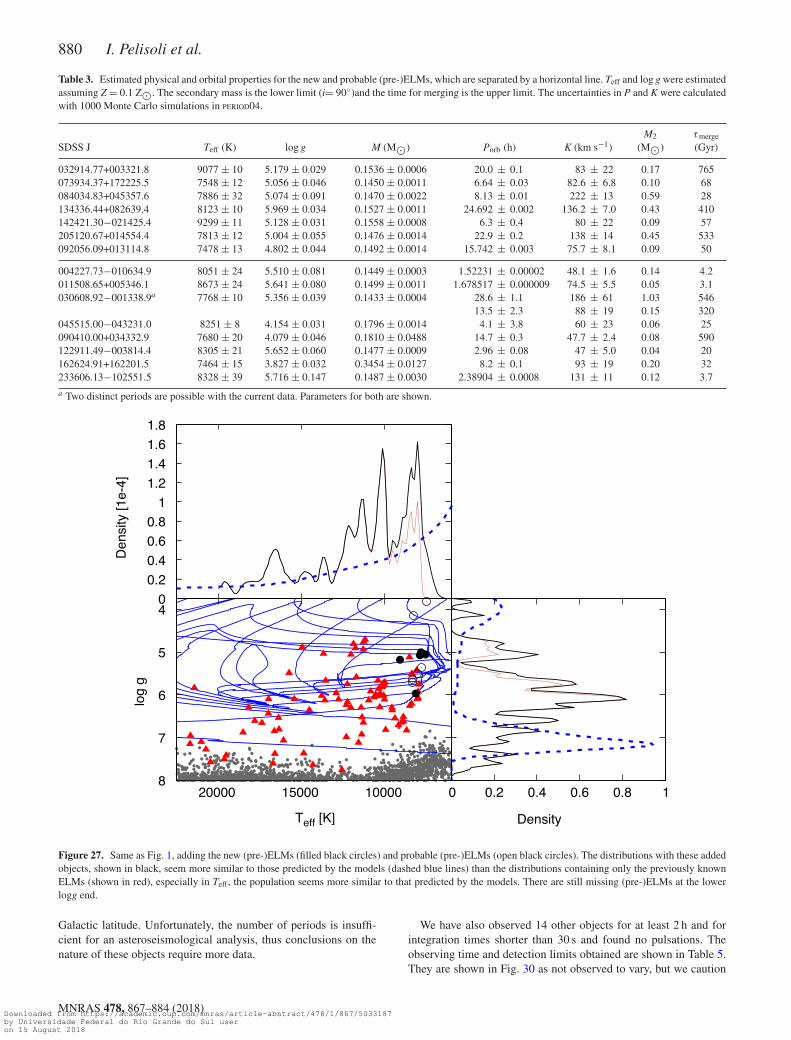
Figure 1. The bottom left panel shows the Teff − log g diagram for objects in the ELM Survey, shown as red triangles, compared with two binary evolutionmodels of Istrate et al. (2016) (blue lines), resulting in ELMs of masses 0.182 and 0.324 M�. The white dwarfs from Kepler et al. (2016) are shown as greydots for comparison. The top panel shows the distributions in Teff, both for the observed ELMs (red continuous line) and obtained from the models (blue dashedline). The bottom right panel shows the distributions for logg. The distributions for the models were obtained taking into account the time spent at each bin ofTeff or log g compared with the total evolutionary time, with a spherical volume correction to account for the difference in brightness (see Pelisoli, Kepler &Koester 2018 for further details). Note that there is a lack of known ELMs at the low Teff and low log g ends of the distribution. There are also missing objectsaround log g ∼ 7.0; however, this range can also be reached through single evolution.
observed every night for flux calibration, except for Gemini obser-vations, which observed one spectrophotometric standard star persemester.
Time series photometry was obtained with the 1.6-m Perkin–Elmer telescope at Observatorio do Pico dos Dias (OPD, Brazil),with an Andor iXon CCD and a red-blocking filter (BG40). We havealso used the imaging mode in Goodman at SOAR for photometry,with the S8612 red-blocking filter. The integration time varied from10–30 s, depending on the brightness of the target, with a typicalreadout of 1–3 s.
2.2 Data analysis
SOAR spectroscopic data were reduced using IRAF’s NOAO package.The frames were first bias-subtracted and flattened with a quartzlamp flat. We then extracted the spectra and performed wavelengthcalibration with a CuHeAr lamp spectrum extracted with the sameaperture. Finally, flux and extinction calibration were applied. TheGEMINI IRAF package was used for data from these telescopes and theX-shooter pipeline for the Very Large Telescope (VLT) data, withequivalent steps in the reduction.
Radial velocity estimates were performed with the XCSAO taskfrom the RVSAO package (Kurtz & Mink 1998), after verifying thatthe intercalated HeAr lamps presented no shift, which was alwaysthe case. We cross-correlated the spectral region covering all visibleBalmer lines (typically from 3750–4900 Å) with spectral templatesfrom the updated model grid based on Koester (2010), described inPelisoli et al. (2018). The values of RV were corrected to the Solarsystem barycentre given the time of observations and the telescopelocation. All our RV estimates are given in Table A1. We have notadded the RVs estimated from the SDSS spectra to our data set,because the SDSS spectra were obtained at least eight years beforeour data, hence the phase might not be accurate with respect to ourrecently obtained data.
We performed a Shapiro–Wilk normality test (Shapiro & Wilk1965) to verify whether the obtained velocities displayed a be-haviour that could be explained by Gaussian uncertainties. Next,we calculated the Lomb–Scargle periodogram (Lomb 1976; Scar-gle 1982) using the NASA Exoplanet Archive tool.1 For each of
1https://exoplanetarchive.ipac.caltech.edu/cgi-bin/Pgram/nph-pgram
MNRAS 478, 867–884 (2018)Downloaded from https://academic.oup.com/mnras/article-abstract/478/1/867/5033187by Universidade Federal do Rio Grande do Sul useron 15 August 2018
870 I. Pelisoli et al.
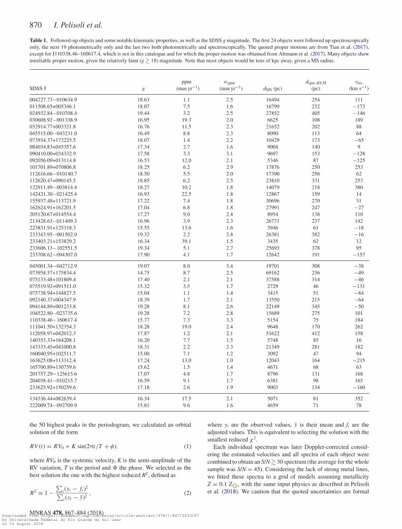
Table 1. Followed-up objects and some notable kinematic properties, as well as the SDSS g magnitude. The first 24 objects were followed up spectroscopicallyonly, the next 19 photometrically only and the last two both photometrically and spectroscopically. The quoted proper motions are from Tian et al. (2017),except for J110338.46–160617.4, which is not in this catalogue and for which the proper motion was obtained from Altmann et al. (2017). Many objects showunreliable proper motion, given the relatively faint (g � 18) magnitude. Note that most objects would be tens of kpc away, given a MS radius.
SDSS J gppm
(mas yr−1)σ ppm
(mas yr−1) dMS (pc)d(pre-)ELM
(pc)vlos
(km s−1)
004227.73−010634.9 18.63 1.1 2.5 16494 254 111011508.65+005346.1 18.07 7.5 1.6 16799 232 −173024932.84−010708.4 19.44 3.2 2.5 27852 405 −146030608.92−001338.9 16.95 19.3 2.0 6625 108 189032914.77+003321.8 16.76 11.5 2.3 21652 202 88045515.00−043231.0 16.49 8.8 2.3 8090 113 64073934.37+172225.5 18.07 1.4 2.2 10429 173 −65084034.83+045357.6 17.34 2.7 1.6 9004 140 9090410.00+034332.9 17.58 3.3 3.1 9697 153 −128092056.09+013114.8 16.53 12.0 2.1 5346 87 −125101701.89+070806.8 18.25 6.2 2.9 17876 250 253112616.66−010140.7 18.50 5.5 2.0 17390 256 62112620.47+090145.5 18.85 6.2 2.5 23810 331 253122911.49−003814.4 18.27 10.2 1.8 14079 218 380142421.30−021425.4 16.93 22.5 1.8 12867 159 14155937.48+113721.9 17.22 7.4 1.8 30696 270 31162624.91+162201.5 17.04 6.8 1.8 27991 247 −27205120.67+014554.4 17.27 9.0 2.4 8954 138 110213428.63−011409.3 16.96 3.9 2.3 26771 237 142223831.91+125318.3 15.55 13.6 1.6 3946 61 −18233343.95−001502.0 19.32 2.2 2.8 26381 382 −16233403.21+153829.2 16.34 39.1 1.5 3435 62 12233606.13−102551.5 19.34 5.1 2.7 25693 378 95233708.62−094307.0 17.90 4.1 1.7 12642 191 −157
045001.34−042712.9 19.07 8.0 3.4 19701 308 −38073958.57+175834.4 14.75 8.7 2.5 69162 236 −49075133.48+101809.4 17.40 2.1 2.1 37588 314 −46075519.92+091511.0 15.32 3.5 1.7 2729 46 −131075738.94+144827.5 15.04 1.1 1.4 3415 51 −84092140.37+004347.9 18.39 1.7 2.1 13550 215 −64094144.89+001233.8 19.28 8.1 2.6 22149 345 −50104522.80−023735.6 19.28 7.2 2.8 15689 275 101110338.46−160617.4 15.77 7.3 3.3 5154 75 184111041.50+132354.3 18.28 19.0 2.4 9648 170 262112058.97+042012.3 17.87 1.2 2.1 51622 412 158140353.33+164208.1 16.20 7.7 1.5 5748 85 16143333.45+041000.8 18.31 2.2 2.3 21349 281 182160040.95+102511.7 15.00 7.1 1.2 3092 47 94163625.08+113312.4 17.24 13.0 1.0 12043 164 −215165700.89+130759.6 15.62 1.5 1.4 4671 68 63201757.29−125615.6 17.07 4.8 1.7 8796 131 168204038.41−010215.7 16.59 9.1 1.7 6381 98 165233625.92+150259.6 17.18 2.6 1.9 9003 134 −160
134336.44+082639.4 16.34 17.5 2.1 5071 81 352222009.74−092709.9 15.81 9.6 1.6 4659 71 78
the 50 highest peaks in the periodogram, we calculated an orbitalsolution of the form
RV (t) = RV0 + K sin(2πt/T + φ), (1)
where RV0 is the systemic velocity, K is the semi-amplitude of theRV variation, T is the period and � the phase. We selected as thebest solution the one with the highest reduced R2, defined as
R2 ≡ 1 −∑
i(yi − fi)2
∑i(yi − y)2
, (2)
where yi are the observed values, y is their mean and fi are theadjusted values. This is equivalent to selecting the solution with thesmallest reduced χ2.
Each individual spectrum was later Doppler-corrected consid-ering the estimated velocities and all spectra of each object werecombined to obtain an S/N� 30 spectrum (the average for the wholesample was S/N = 45). Considering the lack of strong metal lines,we fitted these spectra to a grid of models assuming metallicityZ = 0.1 Z�, with the same input physics as described in Pelisoliet al. (2018). We caution that the quoted uncertainties are formal
MNRAS 478, 867–884 (2018)Downloaded from https://academic.oup.com/mnras/article-abstract/478/1/867/5033187by Universidade Federal do Rio Grande do Sul useron 15 August 2018
The sdA problem – II. Observational follow-up 871
fitting errors and the systematic uncertainties are larger. We previ-ously estimated the systematic uncertainties to be ∼5 per cent inTeff and 0.25 dex in log g (e.g. Pelisoli et al. 2018); however, as wewill show in Section 3.4, it seems that the systematic uncertainty inlog g can actually be higher in the Teff−log g region of the sdAs andcan reach 0.5 dex. The SDSS spectra of all objects were also fittedto the same Z = 0.1 Z� grid to allow a comparison. We have reliedon the SDSS colours to choose between hot and cool solutions withsimilar χ2, which arise due to similar equivalent width being pos-sible with different combinations of Teff and log g. To estimate themass of each object, we interpolated the models of Althaus et al.(2013). The models of Istrate et al. (2016) made a large improve-ment to the input physics, by taking into account rotational mixing,which was shown to be an important factor in the atmosphere abun-dances for ELMs. However, the lowest ELM mass in the models ofIstrate et al. (2016) is 0.16−0.18 M�, depending on the metallicity,and most of our objects show mass lower than that. Only one ob-ject (SDSSJ1626+2622) could have its mass accurately determinedwith the Istrate et al. (2016) models, and this agreed with the massestimate using Althaus et al. (2013) within the uncertainties. Hence,to be consistent, we used the models of Althaus et al. (2013) for allmass estimates.
All photometry images were bias-subtracted and flat-field cor-rected using dome flats. Aperture photometry was performed usingthe DAOPHOT package in IRAF. A neighbouring non-variable star ofsimilar brightness was used to perform differential photometry. Theresulting light curve was analysed with PERIOD04 (Lenz & Breger2005), in search of pulsations with amplitude at least four timeslarger than the average amplitude of the Fourier transform. PERIOD04was also used to fit the light curve and perform pre-whitening whenpulsations were found and to estimate uncertainties using the MonteCarlo method with 1000 simulations.
3 R ESULTS
We found seven objects with RV variations that indicate they arein close binaries. They show p-values smaller than 0.15 for theShapiro–Wilk test, implying that the variations cannot be explainedby Gaussian noise to a confidence level of 85 per cent. For sixobjects out of these seven, the p-value is smaller than 0.05, hencethe confidence level is 95 per cent. The orbital solution shows R2
larger than 0.95 for all but one object. Teff and log g suggest theyare new (pre-)ELMs. Their properties are given in Section 3.1.
For six other objects, the p-value is larger than 0.15, but we obtainan orbital solution with a short period (P � 10 h), expected from(pre-)ELMs in the range of physical parameters for the sdAs (Brownet al. 2017), and R2 � 0.85. Two other objects show p < 0.05, buttheir atmospheric parameters are compatible with both a pre-ELMand a main-sequence star. More data are required to confirm thenature of these eight objects; given the distance modules or propermotion and the estimated physical parameters, we assume they areprobable (pre-)ELMs and discuss their properties in Section 3.2.
Six other objects have 12 measurements or more (the averagenecessary to confirm binarity, according to Brown et al. 2016a),in at least three different epochs and often multiple telescopes, butthe Shapiro–Wilk test suggested no real variation. These objectsare possibly single stars or show either very short (� 1.0 h) orlong periods (� 200 d). We also found no RV variation or redcompanions for the five objects observed with X-shooter in threenights over a week. All these objects are detailed in Section 3.3.
In Section 3.4, we compare the values of Teff and log g obtainedby fitting the SDSS spectra and the SOAR or X-shooter spectra
0
50
100
150
200
250
300
350
0 5 10 15 20 25 30 35 40
RV
(km
/s)
Phase (h)
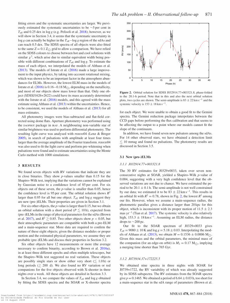
Figure 2. Orbital solution for SDSS J032914.77+003321.8, phase-foldedto the 20.1-h period. Note that in this and also the next orbital solutionplots, two cycles are shown. The semi-amplitude is 83 ± 22 km s−1 and thesystemic velocity is 153 ± 18 km s−1.
for each object. We were unable to obtain a good fit to the Geminispectra. The Gemini reduction package interpolates between theCCD gaps before performing the flux calibration and that seems tobe affecting the output to a point where our models cannot fit theslope of the continuum.
In addition, we have found seven new pulsators among the sdAs.For 14 other observed stars, we have obtained a detection limit� 10 mmag and found no pulsations. The photometry results arediscussed in Section 3.5.
3.1 New (pre-)ELMs
3.1.1 J032914.77+003321.8
The 30 RV estimates for J0329+0033, taken over seven non-consecutive nights at SOAR, yielded a Shapiro–Wilk p-value of0.004, suggesting with a very high confidence level that the ob-served variations are not due to chance. We have estimated the pe-riod to be 20.1 ± 0.1 h. The semi-amplitude is not well constrainedby our data; we estimated it to be 83 ± 22 km s−1. This results inan orbital fit with R2 = 0.78, shown in Fig. 2, the lowest R2 amongour fits. However, when we assume a main-sequence radius, thephotometric parallax gives a distance larger than 20 kpc for thisobject, which is inconsistent with its proper motion of 11.5 ± 2.3mas yr−1 (Tian et al. 2017). The systemic velocity is also relativelyhigh, 153.3 ± 18 km s−1. Assuming an ELM radius, the distancedrops to ∼200 pc.
Our fit to the SOAR spectrum of J0329+0033 givesTeff = 9080 ± 10 K and log g = 5.18 ± 0.03. Interpolating the mod-els of Althaus et al. (2013), we obtain M = 0.1536 ± 0.0006 M�.Given this mass and the orbital parameters, the minimal mass ofthe companion (for an edge-on orbit) is M2 = 0.17 M�, implyinga merging time shorter than 765 Gyr.
3.1.2 J073934.37+172225.5
We obtained nine spectra in three nights with SOAR forJ0739+1722, the RV variability of which was already suggestedby its SDSS subspectra. The RV estimates from the SOAR spectragive p = 0.1465. We obtained a period of 6.64 ± 0.03 h, too short fora main-sequence star in the sdA range of parameters (Brown et al.
MNRAS 478, 867–884 (2018)Downloaded from https://academic.oup.com/mnras/article-abstract/478/1/867/5033187by Universidade Federal do Rio Grande do Sul useron 15 August 2018
872 I. Pelisoli et al.
-100
-50
0
50
100
150
200
0 2 4 6 8 10 12
RV
(km
/s)
Phase (h)
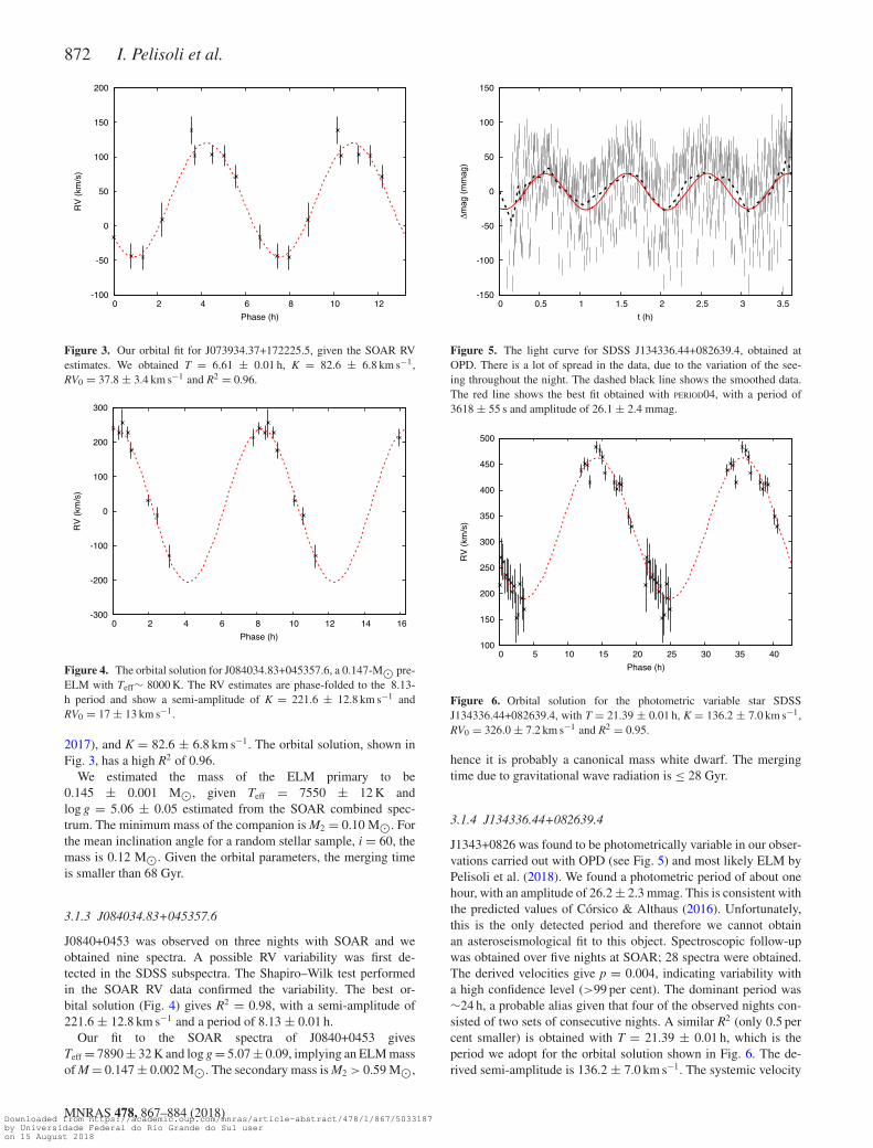
Figure 3. Our orbital fit for J073934.37+172225.5, given the SOAR RVestimates. We obtained T = 6.61 ± 0.01 h, K = 82.6 ± 6.8 km s−1,RV0 = 37.8 ± 3.4 km s−1 and R2 = 0.96.
-300
-200
-100
0
100
200
300
0 2 4 6 8 10 12 14 16
RV
(km
/s)
Phase (h)
Figure 4. The orbital solution for J084034.83+045357.6, a 0.147-M� pre-ELM with Teff∼ 8000 K. The RV estimates are phase-folded to the 8.13-h period and show a semi-amplitude of K = 221.6 ± 12.8 km s−1 andRV0 = 17 ± 13 km s−1.
2017), and K = 82.6 ± 6.8 km s−1. The orbital solution, shown inFig. 3, has a high R2 of 0.96.
We estimated the mass of the ELM primary to be0.145 ± 0.001 M�, given Teff = 7550 ± 12 K andlog g = 5.06 ± 0.05 estimated from the SOAR combined spec-trum. The minimum mass of the companion is M2 = 0.10 M�. Forthe mean inclination angle for a random stellar sample, i = 60, themass is 0.12 M�. Given the orbital parameters, the merging timeis smaller than 68 Gyr.
3.1.3 J084034.83+045357.6
J0840+0453 was observed on three nights with SOAR and weobtained nine spectra. A possible RV variability was first de-tected in the SDSS subspectra. The Shapiro–Wilk test performedin the SOAR RV data confirmed the variability. The best or-bital solution (Fig. 4) gives R2 = 0.98, with a semi-amplitude of221.6 ± 12.8 km s−1 and a period of 8.13 ± 0.01 h.
Our fit to the SOAR spectra of J0840+0453 givesTeff = 7890 ± 32 K and log g = 5.07 ± 0.09, implying an ELM massof M = 0.147 ± 0.002 M�. The secondary mass is M2 > 0.59 M�,
-150
-100
-50
0
50
100
150
0 0.5 1 1.5 2 2.5 3 3.5
Δmag
(m
mag
)
t (h)
Figure 5. The light curve for SDSS J134336.44+082639.4, obtained atOPD. There is a lot of spread in the data, due to the variation of the see-ing throughout the night. The dashed black line shows the smoothed data.The red line shows the best fit obtained with PERIOD04, with a period of3618 ± 55 s and amplitude of 26.1 ± 2.4 mmag.
100
150
200
250
300
350
400
450
500
0 5 10 15 20 25 30 35 40
RV
(km
/s)
Phase (h)
Figure 6. Orbital solution for the photometric variable star SDSSJ134336.44+082639.4, with T = 21.39 ± 0.01 h, K = 136.2 ± 7.0 km s−1,RV0 = 326.0 ± 7.2 km s−1 and R2 = 0.95.
hence it is probably a canonical mass white dwarf. The mergingtime due to gravitational wave radiation is ≤ 28 Gyr.
3.1.4 J134336.44+082639.4
J1343+0826 was found to be photometrically variable in our obser-vations carried out with OPD (see Fig. 5) and most likely ELM byPelisoli et al. (2018). We found a photometric period of about onehour, with an amplitude of 26.2 ± 2.3 mmag. This is consistent withthe predicted values of Corsico & Althaus (2016). Unfortunately,this is the only detected period and therefore we cannot obtainan asteroseismological fit to this object. Spectroscopic follow-upwas obtained over five nights at SOAR; 28 spectra were obtained.The derived velocities give p = 0.004, indicating variability witha high confidence level (>99 per cent). The dominant period was∼24 h, a probable alias given that four of the observed nights con-sisted of two sets of consecutive nights. A similar R2 (only 0.5 percent smaller) is obtained with T = 21.39 ± 0.01 h, which is theperiod we adopt for the orbital solution shown in Fig. 6. The de-rived semi-amplitude is 136.2 ± 7.0 km s−1. The systemic velocity
MNRAS 478, 867–884 (2018)Downloaded from https://academic.oup.com/mnras/article-abstract/478/1/867/5033187by Universidade Federal do Rio Grande do Sul useron 15 August 2018
The sdA problem – II. Observational follow-up 873
-50
0
50
100
150
200
0 2 4 6 8 10 12
RV
(km
/s)
Phase (h)
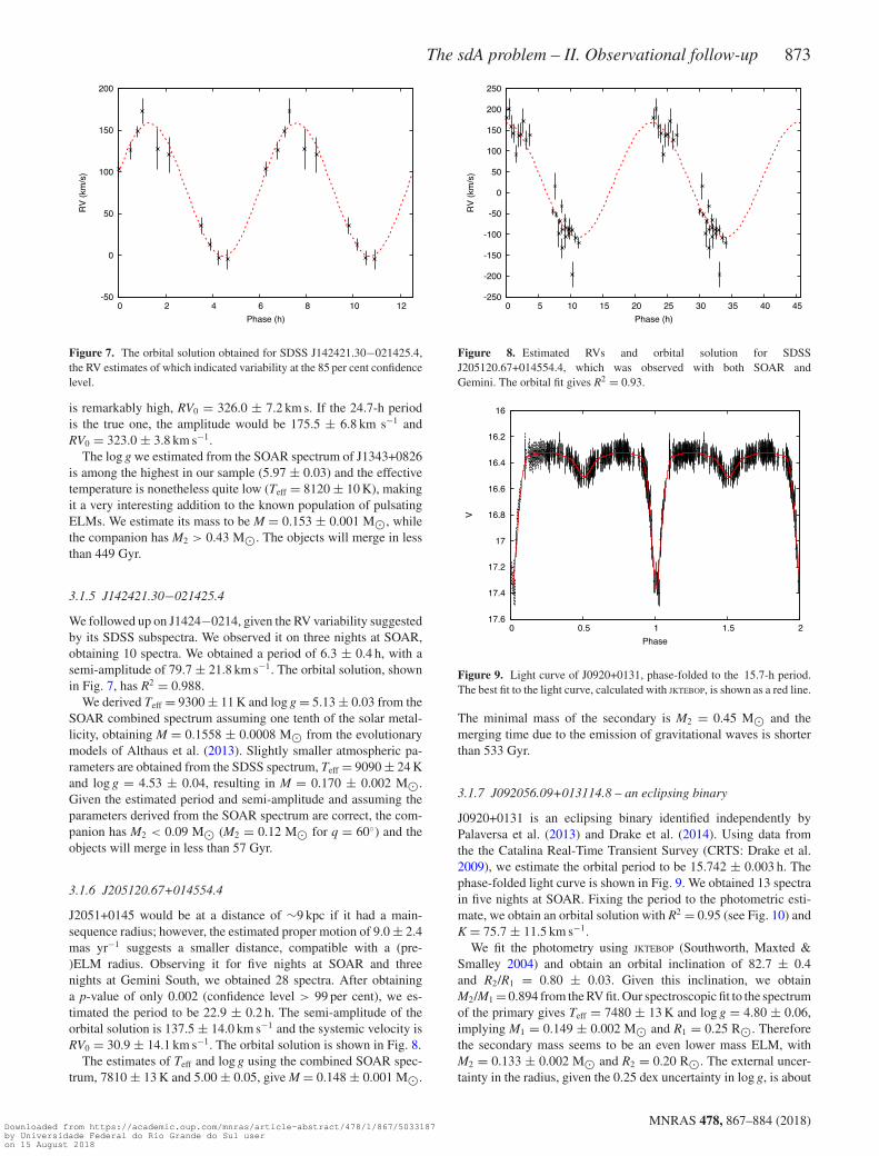
Figure 7. The orbital solution obtained for SDSS J142421.30−021425.4,the RV estimates of which indicated variability at the 85 per cent confidencelevel.
is remarkably high, RV0 = 326.0 ± 7.2 km s. If the 24.7-h periodis the true one, the amplitude would be 175.5 ± 6.8 km s−1 andRV0 = 323.0 ± 3.8 km s−1.
The log g we estimated from the SOAR spectrum of J1343+0826is among the highest in our sample (5.97 ± 0.03) and the effectivetemperature is nonetheless quite low (Teff = 8120 ± 10 K), makingit a very interesting addition to the known population of pulsatingELMs. We estimate its mass to be M = 0.153 ± 0.001 M�, whilethe companion has M2 > 0.43 M�. The objects will merge in lessthan 449 Gyr.
3.1.5 J142421.30−021425.4
We followed up on J1424−0214, given the RV variability suggestedby its SDSS subspectra. We observed it on three nights at SOAR,obtaining 10 spectra. We obtained a period of 6.3 ± 0.4 h, with asemi-amplitude of 79.7 ± 21.8 km s−1. The orbital solution, shownin Fig. 7, has R2 = 0.988.
We derived Teff = 9300 ± 11 K and log g = 5.13 ± 0.03 from theSOAR combined spectrum assuming one tenth of the solar metal-licity, obtaining M = 0.1558 ± 0.0008 M� from the evolutionarymodels of Althaus et al. (2013). Slightly smaller atmospheric pa-rameters are obtained from the SDSS spectrum, Teff = 9090 ± 24 Kand log g = 4.53 ± 0.04, resulting in M = 0.170 ± 0.002 M�.Given the estimated period and semi-amplitude and assuming theparameters derived from the SOAR spectrum are correct, the com-panion has M2 < 0.09 M� (M2 = 0.12 M� for q = 60◦) and theobjects will merge in less than 57 Gyr.
3.1.6 J205120.67+014554.4
J2051+0145 would be at a distance of ∼9 kpc if it had a main-sequence radius; however, the estimated proper motion of 9.0 ± 2.4mas yr−1 suggests a smaller distance, compatible with a (pre-)ELM radius. Observing it for five nights at SOAR and threenights at Gemini South, we obtained 28 spectra. After obtaininga p-value of only 0.002 (confidence level > 99 per cent), we es-timated the period to be 22.9 ± 0.2 h. The semi-amplitude of theorbital solution is 137.5 ± 14.0 km s−1 and the systemic velocity isRV0 = 30.9 ± 14.1 km s−1. The orbital solution is shown in Fig. 8.
The estimates of Teff and log g using the combined SOAR spec-trum, 7810 ± 13 K and 5.00 ± 0.05, give M = 0.148 ± 0.001 M�.
-250
-200
-150
-100
-50
0
50
100
150
200
250
0 5 10 15 20 25 30 35 40 45
RV
(km
/s)
Phase (h)
Figure 8. Estimated RVs and orbital solution for SDSSJ205120.67+014554.4, which was observed with both SOAR andGemini. The orbital fit gives R2 = 0.93.
16
16.2
16.4
16.6
16.8
17
17.2
17.4
17.6 0 0.5 1 1.5 2
V
Phase
Figure 9. Light curve of J0920+0131, phase-folded to the 15.7-h period.The best fit to the light curve, calculated with JKTEBOP, is shown as a red line.
The minimal mass of the secondary is M2 = 0.45 M� and themerging time due to the emission of gravitational waves is shorterthan 533 Gyr.
3.1.7 J092056.09+013114.8 – an eclipsing binary
J0920+0131 is an eclipsing binary identified independently byPalaversa et al. (2013) and Drake et al. (2014). Using data fromthe the Catalina Real-Time Transient Survey (CRTS: Drake et al.2009), we estimate the orbital period to be 15.742 ± 0.003 h. Thephase-folded light curve is shown in Fig. 9. We obtained 13 spectrain five nights at SOAR. Fixing the period to the photometric esti-mate, we obtain an orbital solution with R2 = 0.95 (see Fig. 10) andK = 75.7 ± 11.5 km s−1.
We fit the photometry using JKTEBOP (Southworth, Maxted &Smalley 2004) and obtain an orbital inclination of 82.7 ± 0.4and R2/R1 = 0.80 ± 0.03. Given this inclination, we obtainM2/M1 = 0.894 from the RV fit. Our spectroscopic fit to the spectrumof the primary gives Teff = 7480 ± 13 K and log g = 4.80 ± 0.06,implying M1 = 0.149 ± 0.002 M� and R1 = 0.25 R�. Thereforethe secondary mass seems to be an even lower mass ELM, withM2 = 0.133 ± 0.002 M� and R2 = 0.20 R�. The external uncer-tainty in the radius, given the 0.25 dex uncertainty in log g, is about
MNRAS 478, 867–884 (2018)Downloaded from https://academic.oup.com/mnras/article-abstract/478/1/867/5033187by Universidade Federal do Rio Grande do Sul useron 15 August 2018
874 I. Pelisoli et al.
-50
0
50
100
150
200
0 5 10 15 20 25 30
RV
(km
/s)
Phase (h)
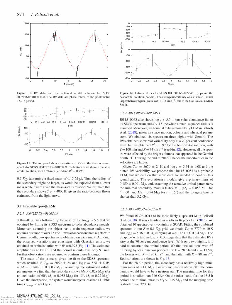
Figure 10. RV data and the obtained orbital solution for SDSSJ092056.09+013114.8. The RV data are phase-folded to the photometric15.7-h period.
-80-40
0 40 80
0 0.1 0.2 0.3 0.4
RV
(km
/s)
810.3 810.6 810.9
t (h)
860.8 861.1
-50
0
50
100
0 0.2 0.4 0.6 0.8 1 1.2 1.4 1.6 1.8 2
Phase
Figure 11. The top panel shows the estimated RVs in the three observedepochs for SDSS J004227.73−010634.9. The bottom panel shows a tentativeorbital solution, with a 91-min periodand R2 = 0.993.
0.7 R� (assuming a fixed mass of 0.15 M�). Thus the radius ofthe secondary might be larger, as would be expected from a lowermass white dwarf given the mass–radius relation. We estimate thatthe secondary shows Teff ∼ 4000 K, given the ratio between fluxesestimated from the light curve.
3.2 Probable (pre-)ELMs
3.2.1 J004227.73−010634.9
J0042–0106 was followed up because of the log g > 5.5 that weobtained by fitting its SDSS spectrum to solar abundance models.Moreover, assuming the object has a main-sequence radius, weobtain a distance of over 15 kpc. It was observed on three nights withGemini South; two spectra were obtained on each night. Althoughthe observed variations are consistent with Gaussian errors, weobtained an orbital solution with R2 = 0.993 (Fig. 11). The estimatedamplitude is 48 km s−1 and the period is quite low, only 91 min.Further observations are required to confirm these findings.
The mass of the primary, given the fit to the SDSS spectrum,which resulted in Teff = 8050 ± 24 and log g = 5.51 ± 0.08,is M = 0.1449 ± 0.0003 M�. Assuming the estimated orbitalparameters, we find that the secondary shows M2 > 0.028 M� (foran inclination of 60◦, M2 = 0.033 M�; for 15◦, M2 = 0.22 M�).Given the short period, the system would merge in less than a Hubbletime (τmerge < 4.2 Gyr).
-250-200-150-100-50
0
0 0.1 0.2
RV
(km
/s) 1175.6 1175.9
t (h)
1243.7 1244
-250
-200
-150
-100
-50
0
0 0.2 0.4 0.6 0.8 1 1.2 1.4 1.6 1.8 2
Phase
Figure 12. Estimated RVs for SDSS J011508.65+005346.1 (top) and thebest orbital solution (bottom). The average uncertainty was 33 km s−1, muchlarger than our typical values of 10–15 km s−1, due to the bias issue at GMOSSouth.
3.2.2 J011508.65+005346.1
J0115+0053 also shows log g > 5.5 in our solar abundance fits toits SDSS spectrum and d > 15 kpc when a main-sequence radius isassumed. Moreover, we found it to be a more likely ELM in Pelisoliet al. (2018), given its space motion, colours and physical param-eters. We obtained six spectra on three nights with Gemini. TheRVs obtained show real variability only at a 70 per cent confidencelevel, but we obtained R2 = 0.97 for the best orbital solution, withT = 100 min and K = 74 km s−1 (see Fig. 12). However, all the spec-tra were affected by the bright columns that appeared in the GeminiSouth CCD during the end of 2016B, hence the uncertainties in thevelocities are larger.
Given Teff = 8670 ± 24 K and log g = 5.64 ± 0.08 and thehinted RV variability, we propose that J0115+0053 is a probableELM, but we caution that more data are needed to confirm thisidentification. The evolutionary models give a primary mass of0.150 ± 0.001 M� and, assuming the tentative orbital parameters,the minimal secondary mass is 0.049 M� (M2 = 0.058 M� fori = 60◦ and M2 = 0.54 M� for i = 15◦) and the merging time isshorter than 3.2 Gyr.
3.2.3 J030608.92−001338.9
We found J0306–0013 to be most likely a (pre-)ELM in Pelisoliet al. (2018). It was classified as a sdA in Kepler et al. (2016). Weobtained 10 spectra over two nights at SOAR. Fitting the combinedspectrum to our Z = 0.1 Z� grid, we obtain Teff = 7770 ± 10 Kand log g = 5.36 ± 0.04, implying M = 0.1433 ± 0.0004 M�. TheShapiro–Wilk test yields p < 0.3, suggesting that the estimated RVsvary at the 70 per cent confidence level. With only two nights, it ishard to constrain the orbital period. We find two solutions with R2
differing by less than two per cent for T = 28.6 h and T = 13.5 h,the former with K = 186 km s−1 and the latter with K = 88 km s−1.Both solutions are shown in Fig. 13.
For the 28.6-h period, the secondary has a relatively high mini-mum mass of ∼1.0 M�. For any inclination above 60◦, the com-panion would have to be a neutron star. The merging time for thisperiod is smaller than 546 Gyr. On the other hand, for the 13.5-hperiod, the minimal mass is M2 > 0.15 M� and the merging timeis shorter than 320 Gyr.
MNRAS 478, 867–884 (2018)Downloaded from https://academic.oup.com/mnras/article-abstract/478/1/867/5033187by Universidade Federal do Rio Grande do Sul useron 15 August 2018
The sdA problem – II. Observational follow-up 875
150
200
250
300
350
0 0.5 1 1.5 2 2.5
RV
(km
/s) t (h)
24 24.5 25 25.5
0
100
200
300
0 0.5 1 1.5 2
Phase
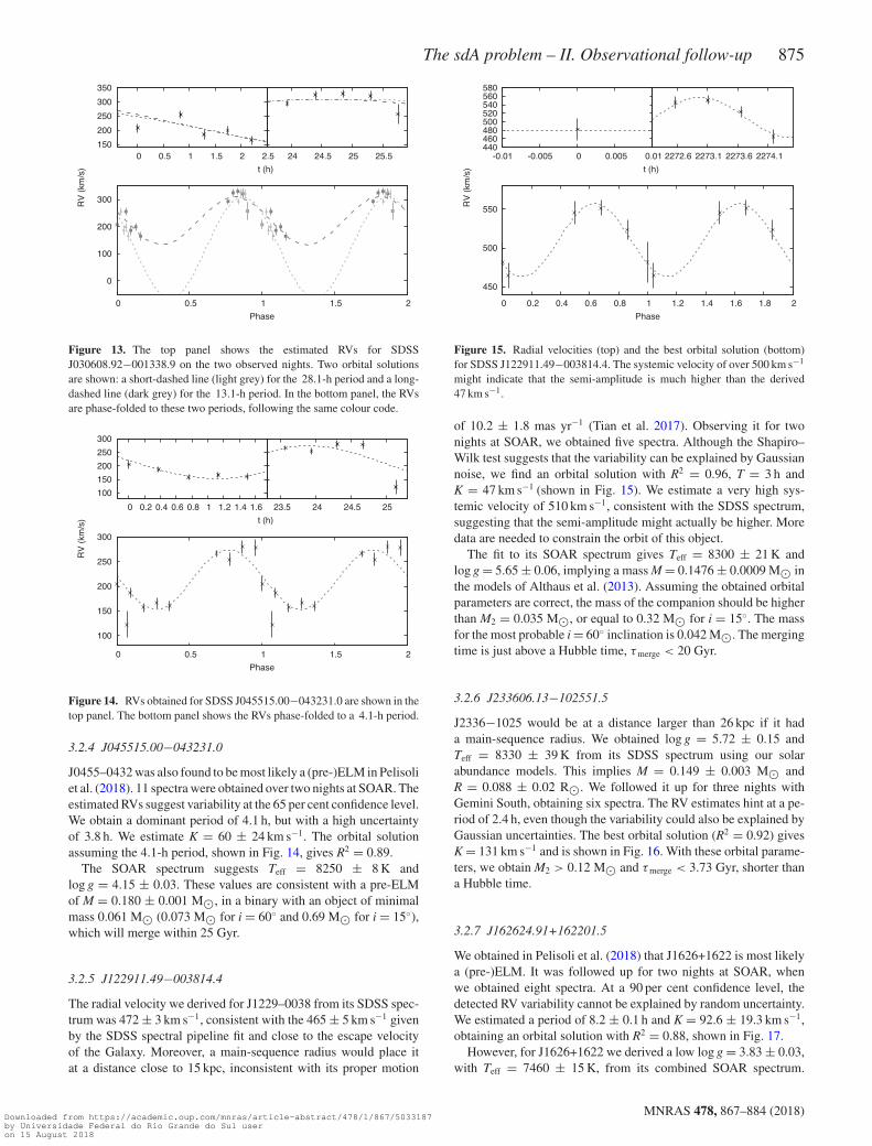
Figure 13. The top panel shows the estimated RVs for SDSSJ030608.92−001338.9 on the two observed nights. Two orbital solutionsare shown: a short-dashed line (light grey) for the 28.1-h period and a long-dashed line (dark grey) for the 13.1-h period. In the bottom panel, the RVsare phase-folded to these two periods, following the same colour code.
100
150
200
250
300
0 0.2 0.4 0.6 0.8 1 1.2 1.4 1.6
RV
(km
/s) t (h)
23.5 24 24.5 25
100
150
200
250
300
0 0.5 1 1.5 2
Phase
Figure 14. RVs obtained for SDSS J045515.00−043231.0 are shown in thetop panel. The bottom panel shows the RVs phase-folded to a 4.1-h period.
3.2.4 J045515.00−043231.0
J0455–0432 was also found to be most likely a (pre-)ELM in Pelisoliet al. (2018). 11 spectra were obtained over two nights at SOAR. Theestimated RVs suggest variability at the 65 per cent confidence level.We obtain a dominant period of 4.1 h, but with a high uncertaintyof 3.8 h. We estimate K = 60 ± 24 km s−1. The orbital solutionassuming the 4.1-h period, shown in Fig. 14, gives R2 = 0.89.
The SOAR spectrum suggests Teff = 8250 ± 8 K andlog g = 4.15 ± 0.03. These values are consistent with a pre-ELMof M = 0.180 ± 0.001 M�, in a binary with an object of minimalmass 0.061 M� (0.073 M� for i = 60◦ and 0.69 M� for i = 15◦),which will merge within 25 Gyr.
3.2.5 J122911.49−003814.4
The radial velocity we derived for J1229–0038 from its SDSS spec-trum was 472 ± 3 km s−1, consistent with the 465 ± 5 km s−1 givenby the SDSS spectral pipeline fit and close to the escape velocityof the Galaxy. Moreover, a main-sequence radius would place itat a distance close to 15 kpc, inconsistent with its proper motion
440 460 480 500 520 540 560 580
-0.01 -0.005 0 0.005 0.01
RV
(km
/s) t (h)
2272.6 2273.1 2273.6 2274.1
450
500
550
0 0.2 0.4 0.6 0.8 1 1.2 1.4 1.6 1.8 2
Phase
Figure 15. Radial velocities (top) and the best orbital solution (bottom)for SDSS J122911.49−003814.4. The systemic velocity of over 500 km s−1
might indicate that the semi-amplitude is much higher than the derived47 km s−1.
of 10.2 ± 1.8 mas yr−1 (Tian et al. 2017). Observing it for twonights at SOAR, we obtained five spectra. Although the Shapiro–Wilk test suggests that the variability can be explained by Gaussiannoise, we find an orbital solution with R2 = 0.96, T = 3 h andK = 47 km s−1 (shown in Fig. 15). We estimate a very high sys-temic velocity of 510 km s−1, consistent with the SDSS spectrum,suggesting that the semi-amplitude might actually be higher. Moredata are needed to constrain the orbit of this object.
The fit to its SOAR spectrum gives Teff = 8300 ± 21 K andlog g = 5.65 ± 0.06, implying a mass M = 0.1476 ± 0.0009 M� inthe models of Althaus et al. (2013). Assuming the obtained orbitalparameters are correct, the mass of the companion should be higherthan M2 = 0.035 M�, or equal to 0.32 M� for i = 15◦. The massfor the most probable i = 60◦ inclination is 0.042 M�. The mergingtime is just above a Hubble time, τmerge < 20 Gyr.
3.2.6 J233606.13−102551.5
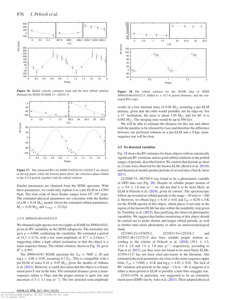
J2336−1025 would be at a distance larger than 26 kpc if it hada main-sequence radius. We obtained log g = 5.72 ± 0.15 andTeff = 8330 ± 39 K from its SDSS spectrum using our solarabundance models. This implies M = 0.149 ± 0.003 M� andR = 0.088 ± 0.02 R�. We followed it up for three nights withGemini South, obtaining six spectra. The RV estimates hint at a pe-riod of 2.4 h, even though the variability could also be explained byGaussian uncertainties. The best orbital solution (R2 = 0.92) givesK = 131 km s−1 and is shown in Fig. 16. With these orbital parame-ters, we obtain M2 > 0.12 M� and τmerge < 3.73 Gyr, shorter thana Hubble time.
3.2.7 J162624.91+162201.5
We obtained in Pelisoli et al. (2018) that J1626+1622 is most likelya (pre-)ELM. It was followed up for two nights at SOAR, whenwe obtained eight spectra. At a 90 per cent confidence level, thedetected RV variability cannot be explained by random uncertainty.We estimated a period of 8.2 ± 0.1 h and K = 92.6 ± 19.3 km s−1,obtaining an orbital solution with R2 = 0.88, shown in Fig. 17.
However, for J1626+1622 we derived a low log g = 3.83 ± 0.03,with Teff = 7460 ± 15 K, from its combined SOAR spectrum.
MNRAS 478, 867–884 (2018)Downloaded from https://academic.oup.com/mnras/article-abstract/478/1/867/5033187by Universidade Federal do Rio Grande do Sul useron 15 August 2018
876 I. Pelisoli et al.
-100 0
100 200 300
0 0.2 0.4
RV
(km
/s) 807.8 808.1 808.4
t (h)
2034.7 2035 2035.3
-150-100
-50 0
50 100 150 200 250 300 350
0 0.2 0.4 0.6 0.8 1 1.2 1.4 1.6 1.8 2
Phase
Figure 16. Radial velocity estimates (top) and the best orbital solution(bottom) for SDSS J233606.13−102551.5.
-120
-80
-40
0
0 0.5 1 1.5 2
RV
(km
/s) t (h)
23.5 24 24.5 25 25.5
-120
-80
-40
0
40
80
0 0.2 0.4 0.6 0.8 1 1.2 1.4 1.6 1.8 2
Phase
Figure 17. The estimated RVs for SDSS J162624.91+162201.5 are shownin the top panel, while the bottom panel shows the velocities phase-foldedto the 8.2-h period, together with the orbital solution.
Similar parameters are obtained from the SDSS spectrum. Withthese parameters, we could only explain it as a pre-ELM in a CNOflash. The time-scale of these flashes ranges from 105–106 years.The estimated physical parameters are consistent with the flashesof a M = 0.34 M� model. Given the estimated orbital parameters,M2 > 0.20 M� and τmerge < 32 Gyr.
3.2.8 J090410.00+034332.9
We obtained eight spectra over two nights at SOAR for J0904+0343,given its RV variability in the SDSS subspectra. The normality testgave p = 0.006, confirming the variability. We estimated a periodof 14.7 ± 0.3 h, with a low semi-amplitude of 47.7 ± 2.4 km s−1,suggesting either a high orbital inclination or that the object is amain-sequence binary. The orbital solution, shown in Fig. 18, givesR2 = 0.997.
The J0904+0343 SOAR spectrum fits Teff = 7680 ± 20 andlog g = 4.08 ± 0.05, assuming 0.1 Z�. This is compatible with apre-ELM of mass 0.18 ± 0.05 M� given the models of Althauset al. (2013). However, it could also mean that the object is a binarymetal-poor F star in the halo. The estimated distance given a main-sequence radius is 9 kpc and the proper motion is quite low anduncertain (3.3 ± 3.1 mas yr−1). The low detected semi-amplitude
-40-20
0 20 40 60 80
100 120
0 0.5 1 1.5
RV
(km
/s) t (h)
24 24.5 25 25.5
-40
-20
0
20
40
60
80
100
120
0 0.5 1 1.5 2
Phase
Figure 18. The orbital solution for the SOAR data of SDSSJ090410.00+034332.9, folded to a 14.7-h period (bottom), and the esti-mated RVs (top).
results in a low minimal mass of 0.08 M� assuming a pre-ELMprimary, given that the orbit would probably not be edge-on. Fora 15◦ inclination, the mass is about 1.05 M� and for 60◦ it is0.092 M�. The merging time would be up to 590 Gyr.
We will be able to estimate the distance for this star and otherswith the parallax to be released by Gaia and therefore the differencebetween our preferred solution as a pre-ELM and a 9-kpc main-sequence star will be clear.
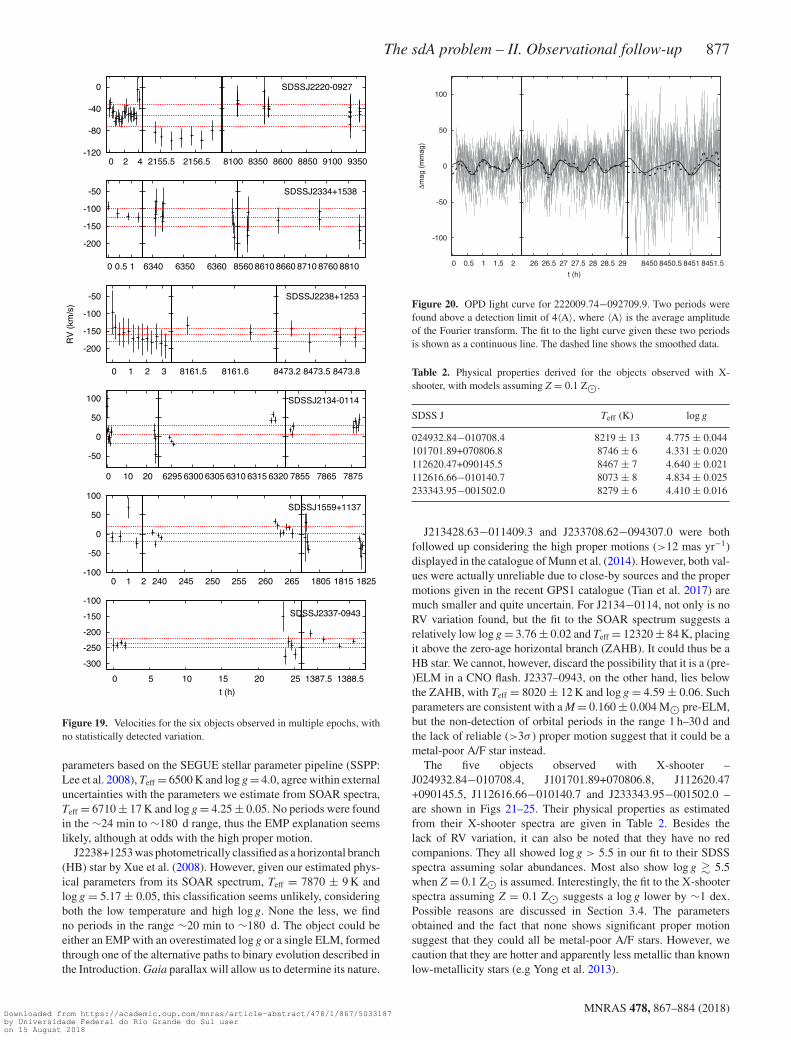
3.3 No detected variation
Fig. 19 shows the RV estimates for those objects with no statisticallysignificant RV variations and no good orbital solutions in the probedranges of periods, described below. We caution that periods as shortas 12 min were observed for the known ELMs (Brown et al. 2011b)and theoretical models predict periods of several days (Sun & Arras2017).
J222009.74−092709.9 was found to be a photometric variablein OPD data (see Fig. 20). Despite its reliable proper motion ofμ = 9.6 ± 1.6 mas yr−1, we did not find it to be most likely anELM in Pelisoli et al. (2018), given its colours. The spectroscopicfollow-up revealed no orbital periods in the range ∼20 min to ∼200d. However, we obtain log g = 6.10 ± 0.02 and Teff = 8230 ± 6 Kfor the SOAR spectra of this object, which places it not only in theregion of the known ELMs but also within the instability strip givenby Tremblay et al. (2015), thus justifying the observed photometricvariability. We suggest that further monitoring of this object shouldbe carried out to probe shorter and longer orbital periods, as wellas further time-series photometry to allow an asteroseismologicalstudy.
J233403.21+153829.2, J223831.91+125318.3 andJ155937.48+113721.9 also have reliable proper motion ac-cording to the criteria of Pelisoli et al. (2018) (39.1 ± 1.5,13.6 ± 1.6 and 7.4 ± 1.8 mas yr−1, respectively, according toTian et al. 2017), yet they were not found to be most likely ELMs.J1559+1137 has not been cited previously in the literature. Ourestimated physical parameters are close to the main-sequence upperlimit, T eff = 11880 ± 41 K and log g = 4.83 ± 0.01. The lack ofRV variation and periods in the range ∼1 h to ∼40 d suggests it iseither a short-period or ELM or possibly a halo blue straggler star.
J2343+1538, in particular, was suggested to be an extremelymetal-poor (EMP) star by Aoki et al. (2013). Their adopted physical
MNRAS 478, 867–884 (2018)Downloaded from https://academic.oup.com/mnras/article-abstract/478/1/867/5033187by Universidade Federal do Rio Grande do Sul useron 15 August 2018
The sdA problem – II. Observational follow-up 877
-120
-80
-40
0
0 2 4 2155.5 2156.5 8100 8350 8600 8850 9100 9350
SDSSJ2220-0927
-200
-150
-100
-50
0 0.5 1 6340 6350 6360 8560 8610 8660 8710 8760 8810
SDSSJ2334+1538
-200
-150
-100
-50
0 1 2 3
RV
(km
/s)
8161.5 8161.6 8473.2 8473.5 8473.8
SDSSJ2238+1253
-50
0
50
100
0 10 20 6295 6300 6305 6310 6315 6320 7855 7865 7875
SDSSJ2134-0114
-100
-50
0
50
100
0 1 2 240 245 250 255 260 265
SDSSJ1559+1137
1805 1815 1825
-300
-250
-200
-150
-100
0 5 10 15 20 25
SDSSJ2337-0943
1387.5 1388.5
t (h)
Figure 19. Velocities for the six objects observed in multiple epochs, withno statistically detected variation.
parameters based on the SEGUE stellar parameter pipeline (SSPP:Lee et al. 2008), Teff = 6500 K and log g = 4.0, agree within externaluncertainties with the parameters we estimate from SOAR spectra,Teff = 6710 ± 17 K and log g = 4.25 ± 0.05. No periods were foundin the ∼24 min to ∼180 d range, thus the EMP explanation seemslikely, although at odds with the high proper motion.
J2238+1253 was photometrically classified as a horizontal branch(HB) star by Xue et al. (2008). However, given our estimated phys-ical parameters from its SOAR spectrum, Teff = 7870 ± 9 K andlog g = 5.17 ± 0.05, this classification seems unlikely, consideringboth the low temperature and high log g. None the less, we findno periods in the range ∼20 min to ∼180 d. The object could beeither an EMP with an overestimated log g or a single ELM, formedthrough one of the alternative paths to binary evolution described inthe Introduction. Gaia parallax will allow us to determine its nature.
-100
-50
0
50
100
0 0.5 1 1.5 2
Δmag
(m
mag
)
26 26.5 27 27.5 28 28.5 29
t (h)
8450 8450.5 8451 8451.5
Figure 20. OPD light curve for 222009.74−092709.9. Two periods werefound above a detection limit of 4〈A〉, where 〈A〉 is the average amplitudeof the Fourier transform. The fit to the light curve given these two periodsis shown as a continuous line. The dashed line shows the smoothed data.
Table 2. Physical properties derived for the objects observed with X-shooter, with models assuming Z = 0.1 Z�.
SDSS J Teff (K) log g
024932.84−010708.4 8219 ± 13 4.775 ± 0.044101701.89+070806.8 8746 ± 6 4.331 ± 0.020112620.47+090145.5 8467 ± 7 4.640 ± 0.021112616.66−010140.7 8073 ± 8 4.834 ± 0.025233343.95−001502.0 8279 ± 6 4.410 ± 0.016
J213428.63−011409.3 and J233708.62−094307.0 were bothfollowed up considering the high proper motions (>12 mas yr−1)displayed in the catalogue of Munn et al. (2014). However, both val-ues were actually unreliable due to close-by sources and the propermotions given in the recent GPS1 catalogue (Tian et al. 2017) aremuch smaller and quite uncertain. For J2134−0114, not only is noRV variation found, but the fit to the SOAR spectrum suggests arelatively low log g = 3.76 ± 0.02 and Teff = 12320 ± 84 K, placingit above the zero-age horizontal branch (ZAHB). It could thus be aHB star. We cannot, however, discard the possibility that it is a (pre-)ELM in a CNO flash. J2337–0943, on the other hand, lies belowthe ZAHB, with Teff = 8020 ± 12 K and log g = 4.59 ± 0.06. Suchparameters are consistent with a M = 0.160 ± 0.004 M� pre-ELM,but the non-detection of orbital periods in the range 1 h–30 d andthe lack of reliable (>3σ ) proper motion suggest that it could be ametal-poor A/F star instead.
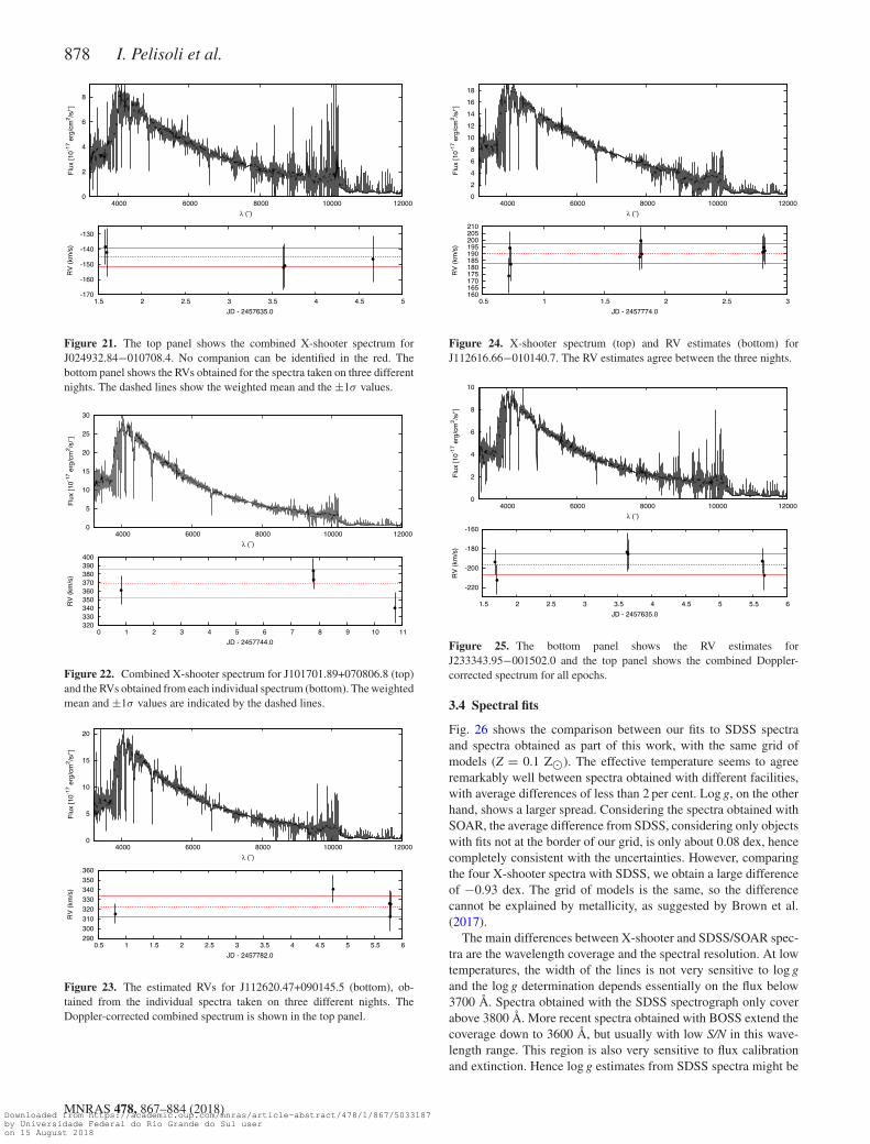
The five objects observed with X-shooter –J024932.84−010708.4, J101701.89+070806.8, J112620.47+090145.5, J112616.66−010140.7 and J233343.95−001502.0 –are shown in Figs 21–25. Their physical properties as estimatedfrom their X-shooter spectra are given in Table 2. Besides thelack of RV variation, it can also be noted that they have no redcompanions. They all showed log g > 5.5 in our fit to their SDSSspectra assuming solar abundances. Most also show log g � 5.5when Z = 0.1 Z� is assumed. Interestingly, the fit to the X-shooterspectra assuming Z = 0.1 Z� suggests a log g lower by ∼1 dex.Possible reasons are discussed in Section 3.4. The parametersobtained and the fact that none shows significant proper motionsuggest that they could all be metal-poor A/F stars. However, wecaution that they are hotter and apparently less metallic than knownlow-metallicity stars (e.g Yong et al. 2013).
MNRAS 478, 867–884 (2018)Downloaded from https://academic.oup.com/mnras/article-abstract/478/1/867/5033187by Universidade Federal do Rio Grande do Sul useron 15 August 2018
878 I. Pelisoli et al.
0
2
4
6
8
4000 6000 8000 10000 12000
Flu
x [1
0-17 e
rg/c
m2 /s
/¯]
λ (¯)
-170
-160
-150
-140
-130
1.5 2 2.5 3 3.5 4 4.5 5
RV
(km
/s)
JD - 2457635.0
Figure 21. The top panel shows the combined X-shooter spectrum forJ024932.84−010708.4. No companion can be identified in the red. Thebottom panel shows the RVs obtained for the spectra taken on three differentnights. The dashed lines show the weighted mean and the ±1σ values.
0
5
10
15
20
25
30
4000 6000 8000 10000 12000
Flu
x [1
0-17 e
rg/c
m2 /s
/¯]
λ (¯)
320 330 340 350 360 370 380 390 400
0 1 2 3 4 5 6 7 8 9 10 11
RV
(km
/s)
JD - 2457744.0
Figure 22. Combined X-shooter spectrum for J101701.89+070806.8 (top)and the RVs obtained from each individual spectrum (bottom). The weightedmean and ±1σ values are indicated by the dashed lines.
0
5
10
15
20
4000 6000 8000 10000 12000
Flu
x [1
0-17 e
rg/c
m2 /s
/¯]
λ (¯)
290 300 310 320 330 340 350 360
0.5 1 1.5 2 2.5 3 3.5 4 4.5 5 5.5 6
RV
(km
/s)
JD - 2457782.0
Figure 23. The estimated RVs for J112620.47+090145.5 (bottom), ob-tained from the individual spectra taken on three different nights. TheDoppler-corrected combined spectrum is shown in the top panel.
0
2
4
6
8
10
12
14
16
18
4000 6000 8000 10000 12000
Flu
x [1
0-17 e
rg/c
m2 /s
/¯]
λ (¯)
160 165 170 175 180 185 190 195 200 205 210
0.5 1 1.5 2 2.5 3
RV
(km
/s)
JD - 2457774.0
Figure 24. X-shooter spectrum (top) and RV estimates (bottom) forJ112616.66−010140.7. The RV estimates agree between the three nights.
0
2
4
6
8
10
4000 6000 8000 10000 12000
Flu
x [1
0-17 e
rg/c
m2 /s
/¯]
λ (¯)
-220
-200
-180
-160
1.5 2 2.5 3 3.5 4 4.5 5 5.5 6
RV
(km
/s)
JD - 2457635.0
Figure 25. The bottom panel shows the RV estimates forJ233343.95−001502.0 and the top panel shows the combined Doppler-corrected spectrum for all epochs.
3.4 Spectral fits
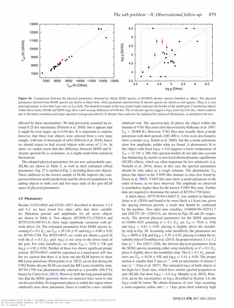
Fig. 26 shows the comparison between our fits to SDSS spectraand spectra obtained as part of this work, with the same grid ofmodels (Z = 0.1 Z�). The effective temperature seems to agreeremarkably well between spectra obtained with different facilities,with average differences of less than 2 per cent. Log g, on the otherhand, shows a larger spread. Considering the spectra obtained withSOAR, the average difference from SDSS, considering only objectswith fits not at the border of our grid, is only about 0.08 dex, hencecompletely consistent with the uncertainties. However, comparingthe four X-shooter spectra with SDSS, we obtain a large differenceof −0.93 dex. The grid of models is the same, so the differencecannot be explained by metallicity, as suggested by Brown et al.(2017).
The main differences between X-shooter and SDSS/SOAR spec-tra are the wavelength coverage and the spectral resolution. At lowtemperatures, the width of the lines is not very sensitive to log gand the log g determination depends essentially on the flux below3700 Å. Spectra obtained with the SDSS spectrograph only coverabove 3800 Å. More recent spectra obtained with BOSS extend thecoverage down to 3600 Å, but usually with low S/N in this wave-length range. This region is also very sensitive to flux calibrationand extinction. Hence log g estimates from SDSS spectra might be
MNRAS 478, 867–884 (2018)Downloaded from https://academic.oup.com/mnras/article-abstract/478/1/867/5033187by Universidade Federal do Rio Grande do Sul useron 15 August 2018
The sdA problem – II. Observational follow-up 879
7000
8000
9000
10000
11000
12000
13000
7000 8000 9000 10000 11000 12000 13000
Tef
f (K
) [S
DS
S]
Teff (K) [Other] 3.5
4
4.5
5
5.5
6
6.5
3.5 4 4.5 5 5.5 6 6.5
log
g [S
DS
S]
log g [Other]
Figure 26. Comparison between the physical parameters obtained by fitting SDSS spectra or SOAR/X-shooter spectra (labelled as other). The physicalparameters derived from SOAR spectra are shown as black dots, while parameters derived from X-shooter spectra are shown as red squares. There is a verygood agreement, to less than 2 per cent, in Teff (left). The dashed rectangle in the log g panel (right) indicates the border of the model grid. Considering objectswithin these limits, SOAR and SDSS logg show a low average difference of 0.08 dex. The X-shooter spectra suggest a log g lower by 0.93 dex, which could bedue to the better resolution and larger spectral coverage provided by X-shooter, but could also be explained by statistical fluctuations, as detailed in the text.
affected by these uncertainties. We had previously assumed an ex-ternal 0.25 dex uncertainty (Pelisoli et al. 2018), but it appears thatit might be even larger, up to 0.50 dex. It is important to caution,however, that these four objects were selected from a very largesample, with tens of thousands of sdAs (Pelisoli et al. 2018), hencewe should expect to find several objects with errors of 2–3σ . Inshort, we cannot assert that this difference between SDSS and X-shooter spectral fits is systematic, as it might result from statisticalfluctuations.
The adopted physical parameters for our new and probable (pre-)ELMs are shown in Table 3, as well as their estimated orbitalparameters. Fig. 27 is similar to Fig. 1, including these new objects.These additions to the known sample of ELMs improve the com-parison between model predictions and the observed population, byadding objects to both cool and low-mass ends of the (pre-)ELMspace of physical parameters.
3.5 Photometry
Besides J1343+0826 and J2220−0927 described in Sections 3.1.4and 3.3, we have found five other sdAs that show variabil-ity. Pulsation periods and amplitudes for all seven objectsare shown in Table 4. Two objects, J073958.57+175834.4 andJ075519.92+091511.0, show large amplitude variations with pe-riods above 2 h. The estimated parameters from SDSS spectra as-suming Z = 0.1 Z� are Teff = 36 136 ± 67 and log g = 6.00 ± 0.02for J0739+1758. For J0755+0915, we could not obtain a good fitwith the Z = 0.1 Z� grid: log g is too close to the lower limit ofthe grid. For solar metallicity, we obtain Teff = 7470 ± 5 K andlog g = 4.50 ± 0.04. Neither of these two shows significant propermotion. J0755+0915 could be explained as a metal-poor A/F star,but we caution that there is at least one pre-ELM known to showRR Lyrae pulsations (Pietrzynski et al. 2012), given that during theCNO flashes the pre-ELM can reach the RR Lyrae instability strip.J0739+1758 was photometrically selected as a possible AM CVnbinary by Carter et al. (2013). However, both the long period and thefact that the SDSS spectrum shows no emission lines seem to ruleout this possibility. Its temperature places it within the region wheresubdwarfs stars show pulsations, hence it could be a new variable
subdwarf star. The spectroscopic fit places the object within thedomain of V361 Hya stars (first discovered by Kilkenny et al. 1997:Teff > 28 000 K). However, V361 Hya stars usually show p-modepulsations with short periods (100–400 s). A few were also found toshow g-modes (e.g. Schuh et al. 2005), but the g-mode pulsationsshow low amplitude, unlike what we found. A photometric fit tothis object with fixed log g = 6.0 suggests a lower temperature ofTeff = 21 745 ± 280. Our spectral models do not take into accountline blanketing by metals or non-local thermodynamic equilibrium(NLTE) effects, which are often important for hot subdwarfs (e.g.Nemeth et al. 2014), hence in this case the spectral parametersshould be only taken as a rough estimate. The photometric Teff
places the object in the V1093 Her domain (a class first found byGreen et al. 2003). V1093 Her stars show g-mode pulsations of theorder of hours, as we have observed. The amplitude we observedis nonetheless higher than for the known V1093 Her stars. Furtherdata are required to determine the nature of J0739+1758 better.
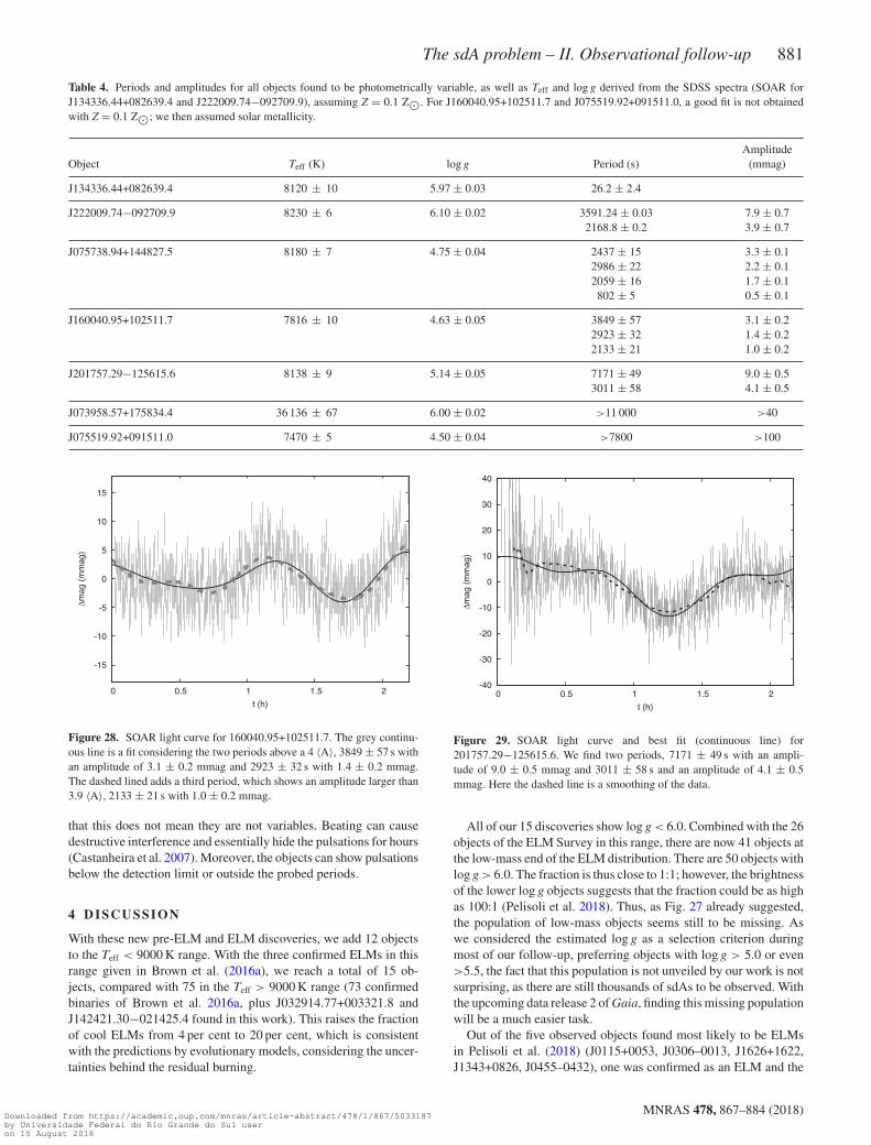
A third object, J075738.94+144827.5, was studied in Sanchez-Arias et al. (2018) and found to be more likely a δ Scuti star, giventhe spacing between periods, a result that should be confirmedby the parallax. Two other new variables, J160040.95+102511.7and J201757.29−125615.6, are shown in Figs 28 and 29, respec-tively. The derived physical parameters for the SDSS spectrumof J1600+1025 assuming Z = 0.1 Z� are Teff = 7816 ± 10 Kand log g = 4.63 ± 0.05, placing it slightly above the instabil-ity strip in Fig. 30. Assuming solar metallicity, the parameters areTeff = 8050 ± 8 K and log g = 5.59 ± 0.03, placing it within the in-stability strip of Tremblay et al. (2015). Its proper motion is 7.1 ± 1.2mas yr−1. For J2017–1256, the derived physical parameters fromthe SDSS spectra assuming either solar metallicity or Z = 0.1 Z�place it slightly above the instability strip. The Z = 0.1 Z� param-eters are Teff = 8138 ± 9 K and log g = 5.14 ± 0.05. The propermotion is smaller than 5 mas yr−1, with an uncertainty of almost 2mas yr−1 (Tian et al. 2017). The estimated log g of both objects istoo high for δ Scuti stars, which have similar spectral properties to(pre-)ELMs, but show log g < 4.4 (e.g. Murphy et al. 2015). How-ever, given the uncertainties in log g described in Section 3.4, thelog g could be lower. We obtain distances of over 3 kpc assuminga main-sequence radius and z > 1 kpc given their relatively high
MNRAS 478, 867–884 (2018)Downloaded from https://academic.oup.com/mnras/article-abstract/478/1/867/5033187by Universidade Federal do Rio Grande do Sul useron 15 August 2018
880 I. Pelisoli et al.
Table 3. Estimated physical and orbital properties for the new and probable (pre-)ELMs, which are separated by a horizontal line. Teff and log g were estimatedassuming Z = 0.1 Z�. The secondary mass is the lower limit (i= 90◦)and the time for merging is the upper limit. The uncertainties in P and K were calculatedwith 1000 Monte Carlo simulations in PERIOD04.
SDSS J Teff (K) log g M (M�) Porb (h) K (km s−1)M2
(M�)τmerge
(Gyr)
032914.77+003321.8 9077 ± 10 5.179 ± 0.029 0.1536 ± 0.0006 20.0 ± 0.1 83 ± 22 0.17 765073934.37+172225.5 7548 ± 12 5.056 ± 0.046 0.1450 ± 0.0011 6.64 ± 0.03 82.6 ± 6.8 0.10 68084034.83+045357.6 7886 ± 32 5.074 ± 0.091 0.1470 ± 0.0022 8.13 ± 0.01 222 ± 13 0.59 28134336.44+082639.4 8123 ± 10 5.969 ± 0.034 0.1527 ± 0.0011 24.692 ± 0.002 136.2 ± 7.0 0.43 410142421.30−021425.4 9299 ± 11 5.128 ± 0.031 0.1558 ± 0.0008 6.3 ± 0.4 80 ± 22 0.09 57205120.67+014554.4 7813 ± 12 5.004 ± 0.055 0.1476 ± 0.0014 22.9 ± 0.2 138 ± 14 0.45 533092056.09+013114.8 7478 ± 13 4.802 ± 0.044 0.1492 ± 0.0014 15.742 ± 0.003 75.7 ± 8.1 0.09 50
004227.73−010634.9 8051 ± 24 5.510 ± 0.081 0.1449 ± 0.0003 1.52231 ± 0.00002 48.1 ± 1.6 0.14 4.2011508.65+005346.1 8673 ± 24 5.641 ± 0.080 0.1499 ± 0.0011 1.678517 ± 0.000009 74.5 ± 5.5 0.05 3.1030608.92−001338.9a 7768 ± 10 5.356 ± 0.039 0.1433 ± 0.0004 28.6 ± 1.1 186 ± 61 1.03 546
13.5 ± 2.3 88 ± 19 0.15 320045515.00−043231.0 8251 ± 8 4.154 ± 0.031 0.1796 ± 0.0014 4.1 ± 3.8 60 ± 23 0.06 25090410.00+034332.9 7680 ± 20 4.079 ± 0.046 0.1810 ± 0.0488 14.7 ± 0.3 47.7 ± 2.4 0.08 590122911.49−003814.4 8305 ± 21 5.652 ± 0.060 0.1477 ± 0.0009 2.96 ± 0.08 47 ± 5.0 0.04 20162624.91+162201.5 7464 ± 15 3.827 ± 0.032 0.3454 ± 0.0127 8.2 ± 0.1 93 ± 19 0.20 32233606.13−102551.5 8328 ± 39 5.716 ± 0.147 0.1487 ± 0.0030 2.38904 ± 0.0008 131 ± 11 0.12 3.7
a Two distinct periods are possible with the current data. Parameters for both are shown.
0
0.2
0.4
0.6
0.8
1
1.2
1.4
1.6
1.8
Den
sity
[1e-
4]
4
5
6
7
8 10000 15000 20000
log
g
Teff [K]
0 0.2 0.4 0.6 0.8 1
Density
Figure 27. Same as Fig. 1, adding the new (pre-)ELMs (filled black circles) and probable (pre-)ELMs (open black circles). The distributions with these addedobjects, shown in black, seem more similar to those predicted by the models (dashed blue lines) than the distributions containing only the previously knownELMs (shown in red), especially in Teff, the population seems more similar to that predicted by the models. There are still missing (pre-)ELMs at the lowerlogg end.
Galactic latitude. Unfortunately, the number of periods is insuffi-cient for an asteroseismological analysis, thus conclusions on thenature of these objects require more data.
We have also observed 14 other objects for at least 2 h and forintegration times shorter than 30 s and found no pulsations. Theobserving time and detection limits obtained are shown in Table 5.They are shown in Fig. 30 as not observed to vary, but we caution
MNRAS 478, 867–884 (2018)Downloaded from https://academic.oup.com/mnras/article-abstract/478/1/867/5033187by Universidade Federal do Rio Grande do Sul useron 15 August 2018
The sdA problem – II. Observational follow-up 881
Table 4. Periods and amplitudes for all objects found to be photometrically variable, as well as Teff and log g derived from the SDSS spectra (SOAR forJ134336.44+082639.4 and J222009.74−092709.9), assuming Z = 0.1 Z�. For J160040.95+102511.7 and J075519.92+091511.0, a good fit is not obtainedwith Z = 0.1 Z�; we then assumed solar metallicity.
Object Teff (K) log g Period (s)Amplitude
(mmag)
J134336.44+082639.4 8120 ± 10 5.97 ± 0.03 26.2 ± 2.4
J222009.74−092709.9 8230 ± 6 6.10 ± 0.02 3591.24 ± 0.03 7.9 ± 0.72168.8 ± 0.2 3.9 ± 0.7
J075738.94+144827.5 8180 ± 7 4.75 ± 0.04 2437 ± 15 3.3 ± 0.12986 ± 22 2.2 ± 0.12059 ± 16 1.7 ± 0.1
802 ± 5 0.5 ± 0.1
J160040.95+102511.7 7816 ± 10 4.63 ± 0.05 3849 ± 57 3.1 ± 0.22923 ± 32 1.4 ± 0.22133 ± 21 1.0 ± 0.2
J201757.29−125615.6 8138 ± 9 5.14 ± 0.05 7171 ± 49 9.0 ± 0.53011 ± 58 4.1 ± 0.5
J073958.57+175834.4 36 136 ± 67 6.00 ± 0.02 >11 000 >40
J075519.92+091511.0 7470 ± 5 4.50 ± 0.04 >7800 >100
-15
-10
-5
0
5
10
15
0 0.5 1 1.5 2
Δmag
(m
mag
)
t (h)
Figure 28. SOAR light curve for 160040.95+102511.7. The grey continu-ous line is a fit considering the two periods above a 4 〈A〉, 3849 ± 57 s withan amplitude of 3.1 ± 0.2 mmag and 2923 ± 32 s with 1.4 ± 0.2 mmag.The dashed lined adds a third period, which shows an amplitude larger than3.9 〈A〉, 2133 ± 21 s with 1.0 ± 0.2 mmag.
that this does not mean they are not variables. Beating can causedestructive interference and essentially hide the pulsations for hours(Castanheira et al. 2007). Moreover, the objects can show pulsationsbelow the detection limit or outside the probed periods.
4 D ISCUSSION
With these new pre-ELM and ELM discoveries, we add 12 objectsto the Teff < 9000 K range. With the three confirmed ELMs in thisrange given in Brown et al. (2016a), we reach a total of 15 ob-jects, compared with 75 in the Teff > 9000 K range (73 confirmedbinaries of Brown et al. 2016a, plus J032914.77+003321.8 andJ142421.30−021425.4 found in this work). This raises the fractionof cool ELMs from 4 per cent to 20 per cent, which is consistentwith the predictions by evolutionary models, considering the uncer-tainties behind the residual burning.
-40
-30
-20
-10
0
10
20
30
40
0 0.5 1 1.5 2
Δmag
(m
mag
)
t (h)
Figure 29. SOAR light curve and best fit (continuous line) for201757.29−125615.6. We find two periods, 7171 ± 49 s with an ampli-tude of 9.0 ± 0.5 mmag and 3011 ± 58 s and an amplitude of 4.1 ± 0.5mmag. Here the dashed line is a smoothing of the data.
All of our 15 discoveries show log g < 6.0. Combined with the 26objects of the ELM Survey in this range, there are now 41 objects atthe low-mass end of the ELM distribution. There are 50 objects withlog g > 6.0. The fraction is thus close to 1:1; however, the brightnessof the lower log g objects suggests that the fraction could be as highas 100:1 (Pelisoli et al. 2018). Thus, as Fig. 27 already suggested,the population of low-mass objects seems still to be missing. Aswe considered the estimated log g as a selection criterion duringmost of our follow-up, preferring objects with log g > 5.0 or even>5.5, the fact that this population is not unveiled by our work is notsurprising, as there are still thousands of sdAs to be observed. Withthe upcoming data release 2 of Gaia, finding this missing populationwill be a much easier task.
Out of the five observed objects found most likely to be ELMsin Pelisoli et al. (2018) (J0115+0053, J0306–0013, J1626+1622,J1343+0826, J0455–0432), one was confirmed as an ELM and the
MNRAS 478, 867–884 (2018)Downloaded from https://academic.oup.com/mnras/article-abstract/478/1/867/5033187by Universidade Federal do Rio Grande do Sul useron 15 August 2018
882 I. Pelisoli et al.
4
5
6
7
8
9 3.9 4 4.1 4.2 4.3 4.4 4.5
log
g
log Teff
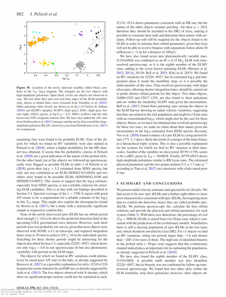
Figure 30. Location of the newly detected variables (filled black sym-bols) in the Teff−log g diagram. The triangles are the two objects withhigh-amplitude pulsations. Open black circles are objects not observed tovary. The hot (blue line) and cool (red line) edges of the ELM instabilitystrip, shown as dotted lines, were extracted from Tremblay et al. (2015).Other pulsating white dwarfs are shown as in fig.1 of Corsico & Althaus(2016): pre-ELMVs (purple), ELMVs (dark grey), DAVs (light grey, bot-tom right), DQVs (green, at log T eff∼ 4.3), DBVs (yellow) and the onlyknown hot DAV (magenta, bottom left). We have also added the sdV starsfrom Holdsworth et al. (2017) (orange) and the newly discovered blue large-amplitude pulsators (BLAPs, shown in cyan) from Pietrukowicz et al. (2017)for comparison.
remaining four were found to be probable ELMs. Four of the ob-jects for which we found no RV variability were also studied inPelisoli et al. (2018), where a higher probability for the MS chan-nel was obtained. It seems that the probability criteria of Pelisoliet al. (2018) are a good indication of the nature of the probed sdAs.On the other hand, ten of the objects we followed up spectroscop-ically were flagged as possible ELMs in table 1 of Pelisoli et al.(2018) given their log g > 5.5 estimated from SDSS spectra, butonly one was confirmed as an ELM (SDSSJ1343+0826) and twoothers were found to be possible ELMs (SDSSJ0042–0106 andSDSSJ0115+0053). This seems to suggest that the log g estimate,especially from SDSS spectra, is not a reliable criterion for select-ing ELM candidates. This is in line with our findings described inSection 3.4. Spectral coverage of the λ < 3700 Å region with goodS/N seems to be a requirement for a reliable estimate of the log gin this Teff range. This might also explain the discrepancies foundby Brown et al. (2017), but a study with a statistically significantsample is required to confirm this.
None of the newly discovered (pre-)ELMs has an orbital periodshort enough (� 1 h) to be above the predicted detection limit of theupcoming LISA gravitational wave detector. However, such shortperiods were not probed by our survey, given that most objects wereobserved with SOAR, a 4.1-m telescope, and required integrationtimes close to 30 min to achieve S/N � 10 in the individual spectra.Searching for these shorter periods might be interesting for theobjects described Section 3.3, especially J2220−0927, which showsnot only log g > 6.0 in our spectroscopic fit but also photometricvariability with periods in the ELM range.
The objects for which we found no RV variations could alterna-tively be metal-poor A/F stars in the halo, as already suggested byBrown et al. (2017) as a possible explanation for sdAs. J2343+1538in particular seems indeed to be an EMP star, as already suggested byAoki et al. (2013). The five objects observed with X-shooter, whichshow no significant proper motion, could also be explained as such.
J2134−0114 shows parameters consistent with an HB star, but thenature of the other objects remains puzzling. All show g < 20.0,therefore they should be included in the DR2 of Gaia, making itpossible to constrain their radii and determine their nature with cer-tainty. Follow-up will still be required for the objects found to beELMs in order to estimate their orbital parameters, given that Gaiawill not be able to resolve binaries with separations below about 20milliarcsec (∼2 au for a distance of 100 pc).
We have also found seven new photometrically variable stars.J1334+0826 was confirmed as an M = 0.15 M� ELM with time-resolved spectroscopy, so it is the eighth member of the ELMVclass, adding to the seven known pulsating ELMs (Hermes et al.2012, 2013a, 2013b; Bell et al. 2015; Kilic et al. 2015). We foundno RV variations for J2220−0927, but its estimated log g and tem-perature place it inside the instability strip, so it is possibly theninth member of the class. Time-resolved spectroscopy with largertelescopes, allowing shorter integration times, should be carried outto probe shorter orbital periods for this object. Two other objects,J1600+1025 and J2017–1256, are also found to show pulsationsand are within the instability ELMV strip given the uncertainties.Bell et al. (2017) found three pulsating stars among the objects inthe ELM Survey showing no radial velocity variations, suggestingthat they are related to the sdA population and might be δ Scuti starswith an overestimated log g, which might also be the case for theseobjects. Hence, as we have not obtained time-resolved spectroscopyfor these two stars, we make no claim about their nature given theuncertainties in the log g estimated from SDSS spectra. Recently,Vos et al. (2018) found evidence of a pre-ELM in a long-period bi-nary (771 ± 3 days), likely the result of a merger of the inner binaryin a hierarchical triple system. This is also a possible explanationfor the systems for which we find no RV variation at short time-scales. Another of the variables we discovered, J0739 +1758, seemsto be a sdBV, given its Teff > 20 000 K. Finally, J0755+0915 showshigh-amplitude pulsations similar to RR Lyrae stars. The estimatedphysical parameters and the low proper motion (3.5 ± 1.7 mas yr−1
according to Tian et al. 2017) are consistent with a halo metal-poorF star.
5 SU M M A RY A N D C O N C L U S I O N S
We present radial velocity estimates and spectral fits for 26 sdAs. Wefind seven to be new (pre-)ELMs and a further eight others to showmost characteristics consistent with (pre-)ELMs, but requiring moredata to confirm the detection, hence they are called probable (pre-)ELMs. We perform spectroscopic fits, calculate the best orbitalsolutions and provide the physical and orbital parameters for eachsystem (Table 3). With these new detections, the percentage of cool(Teff < 9000 K) ELMs is raised from 4 to 20 per cent, which is con-sistent with the predictions of the evolutionary models. Nonethelessthere is still a missing population of (pre-)ELMs at the low-massend, which should be unveiled by Gaia DR2. For 11 objects we findno RV variations, ruling out periods larger than ∼1 h and shorterthan ∼200 d for most of them. The high rate of identified binariesin the probed sdAs (∼58 per cent) suggests that this evolutionarychannel indeed plays an important role in explaining the population,as already suggested in Pelisoli et al. (2018).
We have also found the eighth member of the ELMV class,J1334+0826. A possible ninth member was also identified,J2220−0927, but its binarity was not confirmed by follow-up time-resolved spectroscopy. We found that two other sdAs within theELM instability strip show pulsations; however, other objects ob-
MNRAS 478, 867–884 (2018)Downloaded from https://academic.oup.com/mnras/article-abstract/478/1/867/5033187by Universidade Federal do Rio Grande do Sul useron 15 August 2018
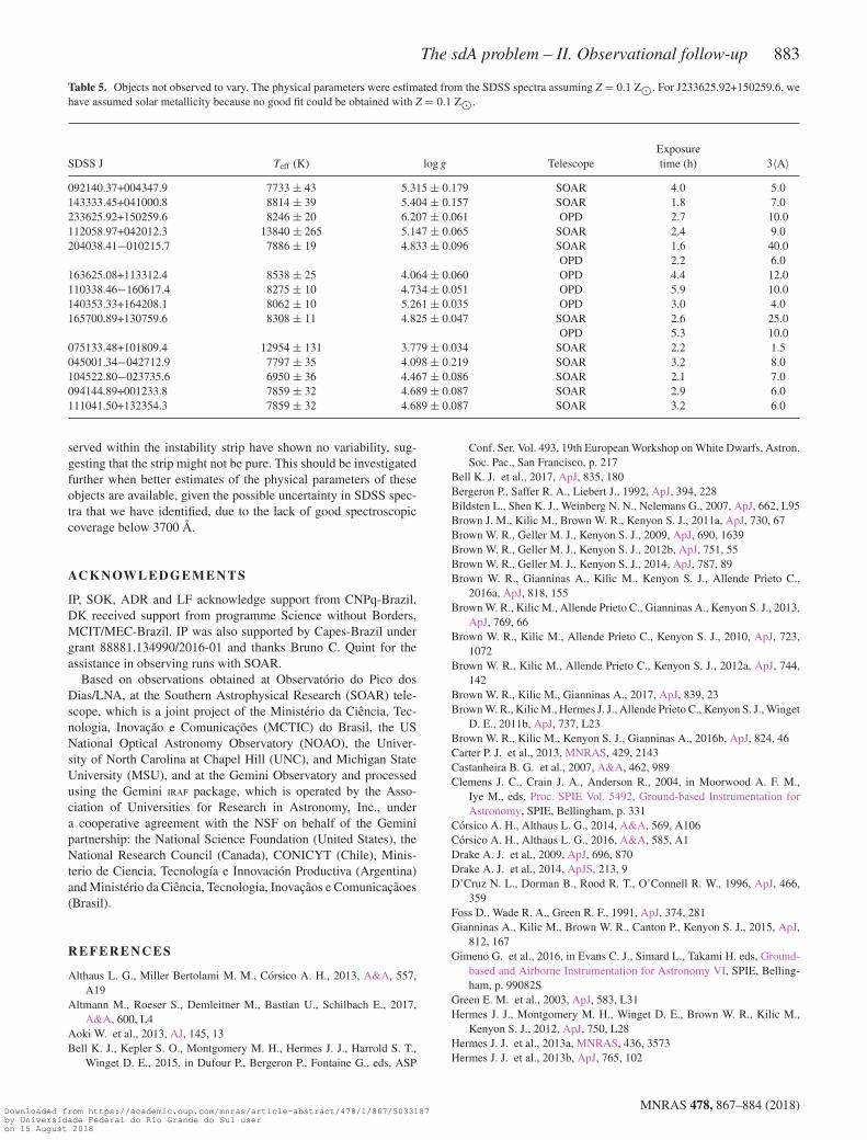
The sdA problem – II. Observational follow-up 883
Table 5. Objects not observed to vary. The physical parameters were estimated from the SDSS spectra assuming Z = 0.1 Z�. For J233625.92+150259.6, wehave assumed solar metallicity because no good fit could be obtained with Z = 0.1 Z�.
SDSS J Teff (K) log g TelescopeExposuretime (h) 3〈A〉
092140.37+004347.9 7733 ± 43 5.315 ± 0.179 SOAR 4.0 5.0143333.45+041000.8 8814 ± 39 5.404 ± 0.157 SOAR 1.8 7.0233625.92+150259.6 8246 ± 20 6.207 ± 0.061 OPD 2.7 10.0112058.97+042012.3 13840 ± 265 5.147 ± 0.065 SOAR 2.4 9.0204038.41−010215.7 7886 ± 19 4.833 ± 0.096 SOAR 1.6 40.0
OPD 2.2 6.0163625.08+113312.4 8538 ± 25 4.064 ± 0.060 OPD 4.4 12.0110338.46−160617.4 8275 ± 10 4.734 ± 0.051 OPD 5.9 10.0140353.33+164208.1 8062 ± 10 5.261 ± 0.035 OPD 3.0 4.0165700.89+130759.6 8308 ± 11 4.825 ± 0.047 SOAR 2.6 25.0
OPD 5.3 10.0075133.48+101809.4 12954 ± 131 3.779 ± 0.034 SOAR 2.2 1.5045001.34−042712.9 7797 ± 35 4.098 ± 0.219 SOAR 3.2 8.0104522.80−023735.6 6950 ± 36 4.467 ± 0.086 SOAR 2.1 7.0094144.89+001233.8 7859 ± 32 4.689 ± 0.087 SOAR 2.9 6.0111041.50+132354.3 7859 ± 32 4.689 ± 0.087 SOAR 3.2 6.0
served within the instability strip have shown no variability, sug-gesting that the strip might not be pure. This should be investigatedfurther when better estimates of the physical parameters of theseobjects are available, given the possible uncertainty in SDSS spec-tra that we have identified, due to the lack of good spectroscopiccoverage below 3700 Å.
AC K N OW L E D G E M E N T S
IP, SOK, ADR and LF acknowledge support from CNPq-Brazil.DK received support from programme Science without Borders,MCIT/MEC-Brazil. IP was also supported by Capes-Brazil undergrant 88881.134990/2016-01 and thanks Bruno C. Quint for theassistance in observing runs with SOAR.
Based on observations obtained at Observatorio do Pico dosDias/LNA, at the Southern Astrophysical Research (SOAR) tele-scope, which is a joint project of the Ministerio da Ciencia, Tec-nologia, Inovacao e Comunicacoes (MCTIC) do Brasil, the USNational Optical Astronomy Observatory (NOAO), the Univer-sity of North Carolina at Chapel Hill (UNC), and Michigan StateUniversity (MSU), and at the Gemini Observatory and processedusing the Gemini IRAF package, which is operated by the Asso-ciation of Universities for Research in Astronomy, Inc., undera cooperative agreement with the NSF on behalf of the Geminipartnership: the National Science Foundation (United States), theNational Research Council (Canada), CONICYT (Chile), Minis-terio de Ciencia, Tecnologıa e Innovacion Productiva (Argentina)and Ministerio da Ciencia, Tecnologia, Inovacaos e Comunicacaoes(Brasil).
RE F EREN C ES
Althaus L. G., Miller Bertolami M. M., Corsico A. H., 2013, A&A, 557,A19
Altmann M., Roeser S., Demleitner M., Bastian U., Schilbach E., 2017,A&A, 600, L4
Aoki W. et al., 2013, AJ, 145, 13Bell K. J., Kepler S. O., Montgomery M. H., Hermes J. J., Harrold S. T.,
Winget D. E., 2015, in Dufour P., Bergeron P., Fontaine G., eds, ASP
Conf. Ser. Vol. 493, 19th European Workshop on White Dwarfs, Astron.Soc. Pac., San Francisco, p. 217
Bell K. J. et al., 2017, ApJ, 835, 180Bergeron P., Saffer R. A., Liebert J., 1992, ApJ, 394, 228Bildsten L., Shen K. J., Weinberg N. N., Nelemans G., 2007, ApJ, 662, L95Brown J. M., Kilic M., Brown W. R., Kenyon S. J., 2011a, ApJ, 730, 67Brown W. R., Geller M. J., Kenyon S. J., 2009, ApJ, 690, 1639Brown W. R., Geller M. J., Kenyon S. J., 2012b, ApJ, 751, 55Brown W. R., Geller M. J., Kenyon S. J., 2014, ApJ, 787, 89Brown W. R., Gianninas A., Kilic M., Kenyon S. J., Allende Prieto C.,
2016a, ApJ, 818, 155Brown W. R., Kilic M., Allende Prieto C., Gianninas A., Kenyon S. J., 2013,
ApJ, 769, 66Brown W. R., Kilic M., Allende Prieto C., Kenyon S. J., 2010, ApJ, 723,
1072Brown W. R., Kilic M., Allende Prieto C., Kenyon S. J., 2012a, ApJ, 744,
142Brown W. R., Kilic M., Gianninas A., 2017, ApJ, 839, 23Brown W. R., Kilic M., Hermes J. J., Allende Prieto C., Kenyon S. J., Winget
D. E., 2011b, ApJ, 737, L23Brown W. R., Kilic M., Kenyon S. J., Gianninas A., 2016b, ApJ, 824, 46Carter P. J. et al., 2013, MNRAS, 429, 2143Castanheira B. G. et al., 2007, A&A, 462, 989Clemens J. C., Crain J. A., Anderson R., 2004, in Moorwood A. F. M.,
Iye M., eds, Proc. SPIE Vol. 5492, Ground-based Instrumentation forAstronomy, SPIE, Bellingham, p. 331
Corsico A. H., Althaus L. G., 2014, A&A, 569, A106Corsico A. H., Althaus L. G., 2016, A&A, 585, A1Drake A. J. et al., 2009, ApJ, 696, 870Drake A. J. et al., 2014, ApJS, 213, 9D’Cruz N. L., Dorman B., Rood R. T., O’Connell R. W., 1996, ApJ, 466,
359Foss D., Wade R. A., Green R. F., 1991, ApJ, 374, 281Gianninas A., Kilic M., Brown W. R., Canton P., Kenyon S. J., 2015, ApJ,
812, 167Gimeno G. et al., 2016, in Evans C. J., Simard L., Takami H. eds, Ground-
based and Airborne Instrumentation for Astronomy VI, SPIE, Belling-ham, p. 99082S
Green E. M. et al., 2003, ApJ, 583, L31Hermes J. J., Montgomery M. H., Winget D. E., Brown W. R., Kilic M.,
Kenyon S. J., 2012, ApJ, 750, L28Hermes J. J. et al., 2013a, MNRAS, 436, 3573Hermes J. J. et al., 2013b, ApJ, 765, 102
MNRAS 478, 867–884 (2018)Downloaded from https://academic.oup.com/mnras/article-abstract/478/1/867/5033187by Universidade Federal do Rio Grande do Sul useron 15 August 2018
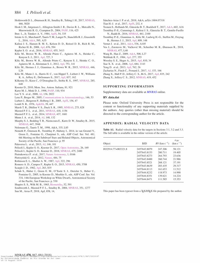
884 I. Pelisoli et al.
Holdsworth D. L., Østensen R. H., Smalley B., Telting J. H., 2017, MNRAS,466, 5020
Hook I. M., Jørgensen I., Allington-Smith J. R., Davies R. L., Metcalfe N.,Murowinski R. G., Crampton D., 2004, PASP, 116, 425
Iben I.,, Jr, Tutukov A. V., 1984, ApJS, 54, 335Istrate A. G., Marchant P., Tauris T. M., Langer N., Stancliffe R. J., Grassitelli
L., 2016, A&A, 595, A35Kalirai J. S., Hansen B. M. S., Kelson D. D., Reitzel D. B., Rich R. M.,
Richer H. B., 2008, ApJ, 676, 594Kepler S. O. et al., 2016, MNRAS, 455, 3413Kilic M., Brown W. R., Allende Prieto C., Agueros M. A., Heinke C.,
Kenyon S. J., 2011, ApJ, 727, 3Kilic M., Brown W. R., Allende Prieto C., Kenyon S. J., Heinke C. O.,
Agueros M. A., Kleinman S. J., 2012, ApJ, 751, 141Kilic M., Hermes J. J., Gianninas A., Brown W. R., 2015, MNRAS, 446,
L26Kilic M., Munn J. A., Harris H. C., von Hippel T., Liebert J. W., Williams
K. A., Jeffery E., DeGennaro S., 2017, ApJ, 837, 162Kilkenny D., Koen C., O’Donoghue D., Stobie R. S., 1997, MNRAS, 285,
640Koester D., 2010, Mem. Soc. Astron. Italiana, 81, 921Kurtz M. J., Mink D. J., 1998, PASP, 110, 934Lee Y. S. et al., 2008, AJ, 136, 2022Lenz P., Breger M., 2005, Communications in Asteroseismology, 146, 53Liebert J., Bergeron P., Holberg J. B., 2005, ApJS, 156, 47Lomb N. R., 1976, Ap&SS, 39, 447Marsh T. R., Dhillon V. S., Duck S. R., 1995, MNRAS, 275, 828Maxted P. F. L. et al., 2011, MNRAS, 418, 1156Maxted P. F. L. et al., 2014, MNRAS, 437, 1681Munn J. A. et al., 2014, AJ, 148, 132Murphy S. J., Bedding T. R., Niemczura E., Kurtz D. W., Smalley B., 2015,
MNRAS, 447, 3948Nelemans G., Tauris T. M., 1998, A&A, 335, L85Nemeth P., Ostensen R., Tremblay P., Hubeny I., 2014, in van Grootel V.,
Green E., Fontaine G., Charpinet S., eds, ASP Conf. Ser. Vol. 481,6th Meeting on Hot Subdwarf Stars and Related Objects, AstronomicalSociety of the Pacific, San Francisco. p. 95
Palaversa L. et al., 2013, AJ, 146, 101Pelisoli I., Kepler S. O., Koester D., 2017, Open Astronomy, 26, 169Pelisoli I., Kepler S. O., Koester D., 2018, MNRAS, 475, 2480Pietrukowicz P. et al., 2017, Nature Astronomy, 1, 0166Pietrzynski G. et al., 2012, Nature, 484, 75Robinson E. L., Shafter A. W., 1987, ApJ, 322, 296Romero A. D., Campos F., Kepler S. O., 2015, MNRAS, 450, 3708Scargle J. D., 1982, ApJ, 263, 835Schuh S., Huber J., Green E. M., O’Toole S. J., Dreizler S., Heber U.,
Fontaine G., 2005, in Koester D., Moehler S., eds, ASP Conf. Ser. Vol.334, 14th European Workshop on White Dwarfs, Astronomical Societyof the Pacific, San Francisco. p. 530
Shapiro S. S., Wilk M. B., 1965, Biometrika, 52, 591Southworth J., Maxted P. F. L., Smalley B., 2004, MNRAS, 351, 1277Sun M., Arras P., 2018, ApJ, 858, 14,
Sanchez-Arias J. P. et al., 2018, A&A, arXiv:1804.07318Tian H.-J. et al., 2017, ApJS, 232, 4Toonen S., Hollands M., Gansicke B. T., Boekholt T., 2017, A&A, 602, A16Tremblay P.-E., Cummings J., Kalirai J. S., Gansicke B. T., Gentile-Fusillo
N., Raddi R., 2016, MNRAS, 461, 2100Tremblay P.-E., Gianninas A., Kilic M., Ludwig H.-G., Steffen M., Freytag
B., Hermes J. J., 2015, ApJ, 809, 148Vernet J. et al., 2011, A&A, 536, A105Vos J., Zorotovic M., Vuckovic M., Schreiber M. R., Østensen R., 2018,
MNRAS, 477, L40Wang B., Han Z., 2009, A&A, 508, L27Webbink R. F., 1984, ApJ, 277, 355Woosley S. E., Heger A., 2015, ApJ, 810, 34Xue X. X. et al., 2008, ApJ, 684, 1143Yong D. et al., 2013, ApJ, 762, 26Zacharias N., Finch C., Frouard J., 2017, AJ, 153, 166Zhang X., Hall P. D., Jeffery C. S., Bi S., 2017, ApJ, 835, 242Zhang X., Jeffery C. S., 2012, MNRAS, 419, 452
SUPPORTI NG INFORMATI ON
Supplementary data are available at MNRAS online.
RV data.dat
Please note: Oxford University Press is not responsible for thecontent or functionality of any supporting materials supplied bythe authors. Any queries (other than missing material) should bedirected to the corresponding author for the article.
APPENDI X: RADI AL VELOCI TY DATA
Table A1. Radial velocity data for the targets in Sections 3.1, 3.2 and 3.3.The full table is available in the online version of the article.
Object BJD RV (km s−1)σRV
(km s−1)
J032914.77+003321.8 2457643.8079 247.306 58.1212457643.8153 280.711 19.4052457643.8273 264.793 23.6362457643.8400 260.744 21.9862457643.8521 268.121 37.1912457643.8639 203.435 29.3172457644.8113 161.653 11.5122457644.8232 118.973 14.9902457644.8351 139.621 14.2242457644.8471 111.585 15.353
This paper has been typeset from a TEX/LATEX file prepared by the author.
MNRAS 478, 867–884 (2018)Downloaded from https://academic.oup.com/mnras/article-abstract/478/1/867/5033187by Universidade Federal do Rio Grande do Sul useron 15 August 2018


![ASTRONOMY AND Spectroscopic and photometric …aa.springer.de/papers/8337002/2300447.pdf · 4m [mmag] 1.5 12 12 epochs was acquired for all objects in the Hipparcos Catalogue (obtained](https://img.pdfslide.net/doc/110x75/6040dfcff8447848b65acdc8/astronomy-and-spectroscopic-and-photometric-aa-4m-mmag-15-12-12-epochs-was-acquired.jpg)