Embed Size (px)
Citation preview
The College of Wooster LibrariesOpen Works
Senior Independent Study Theses
2017
The Search for GTO: Determining Optimal PokerStrategy Using Linear ProgrammingStuart YoungThe College of Wooster, [email protected]
Follow this and additional works at: https://openworks.wooster.edu/independentstudy
This Senior Independent Study Thesis Exemplar is brought to you by Open Works, a service of The College of Wooster Libraries. It has been acceptedfor inclusion in Senior Independent Study Theses by an authorized administrator of Open Works. For more information, please [email protected].
© Copyright 2017 Stuart Young
Recommended CitationYoung, Stuart, "The Search for GTO: Determining Optimal Poker Strategy Using Linear Programming" (2017). Senior IndependentStudy Theses. Paper 7807.https://openworks.wooster.edu/independentstudy/7807

The Search for GTO:Determining Optimal Poker
Strategy Using LinearProgramming
Independent Study Thesis
Presented in Partial Fulfillment of theRequirements for the Degree Bachelor of Arts inthe Department of Mathematics and Computer
Science at The College of Wooster
byStuart Young
The College of Wooster2017
Advised by:
Dr. Matthew Moynihan

Abstract
This project applies techniques from game theory and linear programming
to find the optimal strategies of two variants of poker. A set of optimal poker
strategies describe a Nash equilibrium, where no player can improve their
outcome by changing their own strategy, given the strategies of their
opponent(s). We first consider Kuhn Poker as a simple application of our
methodology. We then turn our attention to 2-7 Draw Poker, a modern variant
onto which little previous research is focused. However, the techniques that
we use are incapable of solving large, full-scale variants of poker such as 2-7
Draw. Therefore, we utilize several abstractions techniques to render a
computationally-feasible LP that retains the underlying spirit of the game. We
use the Gambit software package to build and solve LPs whose solutions are
the optimal strategies for each game.
iii


Acknowledgements
To my advisor, Dr. Moynihan, thank you. You have consistently pushed
me to achieve, and have remained supportive during difficult moments. You
have furthered my abilities in mathematics, critical thinking, and writing;
these are skills I will always value.
To my parents, Lee Stivers and Peter Young, thank you. Beyond just
providing me with this education, you taught me why its so important. Mom,
you have inspired my love of scientific inquiry and desire for new knowledge.
Most importantly, you are supportive, reassuring, and always there for me.
To my friend and roommate, Parker Ohlmann, thank you. Your constant
support over the last 4 years has been invaluable, as you remind me to keep all
of this in perspective. I am inspired every day by your dedication,
compassion, and kindness in life.
This project, and my time at the College of Wooster, would not have been
possible without each of you.
v

Contents
Abstract iii
Acknowledgements v
1 Introduction 1
2 Linear Programming 3
2.1 Basic Theory . . . . . . . . . . . . . . . . . . . . . . . . . . . . . . . 4
2.1.1 Constraints . . . . . . . . . . . . . . . . . . . . . . . . . . . 4
2.1.2 Solutions . . . . . . . . . . . . . . . . . . . . . . . . . . . . . 7
2.2 Duality . . . . . . . . . . . . . . . . . . . . . . . . . . . . . . . . . . 9
2.2.1 Motivation . . . . . . . . . . . . . . . . . . . . . . . . . . . . 9
2.2.2 Theory . . . . . . . . . . . . . . . . . . . . . . . . . . . . . . 12
3 Game Theory 17
3.1 Background . . . . . . . . . . . . . . . . . . . . . . . . . . . . . . . 17
3.2 Normal (Strategic) Form . . . . . . . . . . . . . . . . . . . . . . . . 19
3.2.1 Equilibrium . . . . . . . . . . . . . . . . . . . . . . . . . . . 23
vii
viii CONTENTS
3.3 Extensive Form . . . . . . . . . . . . . . . . . . . . . . . . . . . . . 30
3.3.1 Perfect Information . . . . . . . . . . . . . . . . . . . . . . . 30
3.3.2 Imperfect Information . . . . . . . . . . . . . . . . . . . . . 36
3.3.3 Nash Equilibrium . . . . . . . . . . . . . . . . . . . . . . . . 40
3.4 Sequence Form . . . . . . . . . . . . . . . . . . . . . . . . . . . . . 41
3.4.1 Linear Programming Theory . . . . . . . . . . . . . . . . . 48
4 Kuhn Poker 55
4.1 Rules . . . . . . . . . . . . . . . . . . . . . . . . . . . . . . . . . . . 55
4.2 Extensive Form . . . . . . . . . . . . . . . . . . . . . . . . . . . . . 56
4.3 Normal Form . . . . . . . . . . . . . . . . . . . . . . . . . . . . . . 56
4.3.1 Strategies . . . . . . . . . . . . . . . . . . . . . . . . . . . . 58
4.3.2 Payoffs . . . . . . . . . . . . . . . . . . . . . . . . . . . . . . 61
4.3.3 Player 1’s Optimal Strategy . . . . . . . . . . . . . . . . . . 62
4.3.4 Player 2’s Optimal Strategy . . . . . . . . . . . . . . . . . . 69
4.4 Sequence Form . . . . . . . . . . . . . . . . . . . . . . . . . . . . . 72
4.4.1 Sequences and Information Sets . . . . . . . . . . . . . . . 72
4.4.2 Payoffs . . . . . . . . . . . . . . . . . . . . . . . . . . . . . . 74
4.4.3 Strategy Constraint Matrices and Realization Plans . . . . 77
4.4.4 Player 2’s Optimal Strategy . . . . . . . . . . . . . . . . . . 79
4.4.5 Player 1’s Optimal Strategy . . . . . . . . . . . . . . . . . . 83
5 2-7 Draw Poker 89
5.1 Rules . . . . . . . . . . . . . . . . . . . . . . . . . . . . . . . . . . . 89
5.2 Abstractions . . . . . . . . . . . . . . . . . . . . . . . . . . . . . . . 92
5.2.1 Deck Reduction . . . . . . . . . . . . . . . . . . . . . . . . . 92
5.2.2 Betting Abstractions . . . . . . . . . . . . . . . . . . . . . . 93
5.2.3 Bucketing . . . . . . . . . . . . . . . . . . . . . . . . . . . . 94
5.3 Simulation . . . . . . . . . . . . . . . . . . . . . . . . . . . . . . . . 98
5.4 Results . . . . . . . . . . . . . . . . . . . . . . . . . . . . . . . . . . 105
5.4.1 2 Initial Buckets . . . . . . . . . . . . . . . . . . . . . . . . . 105
5.4.2 3 Initial Buckets . . . . . . . . . . . . . . . . . . . . . . . . . 109
6 Conclusion 111
A Gambit 113
B Simplified 2-7 Draw LP Results 117

List of Figures
3.1 Generalized Two-player Strategic Game . . . . . . . . . . . . . . . 22
3.2 Prisoner’s Dilemma . . . . . . . . . . . . . . . . . . . . . . . . . . . 24
3.3 Extensive Form Game with Perfect Information . . . . . . . . . . . 33
3.4 Extensive Form Game with Imperfect Information and Perfect
Recall . . . . . . . . . . . . . . . . . . . . . . . . . . . . . . . . . . . 38
3.5 Sequence Form Example . . . . . . . . . . . . . . . . . . . . . . . . 45
4.1 Extensive Form of Kuhn Poker . . . . . . . . . . . . . . . . . . . . 57
4.2 Player 1’s pure strategies in Kuhn Poker . . . . . . . . . . . . . . . 59
4.3 Player 2’s pure strategies in Kuhn Poker . . . . . . . . . . . . . . . 60
4.4 Subtree of Kuhn Poker . . . . . . . . . . . . . . . . . . . . . . . . . 73
4.5 Payoff function example, with g(s∅, sa, sm) = −1 shown in blue. . . 75
5.1 Initial Transition Probabilities to 2 Buckets . . . . . . . . . . . . . . 97
5.2 Initial Transition Probabilities to 3 Buckets . . . . . . . . . . . . . . 97
5.3 Final Transition Probabilities from 2 Buckets . . . . . . . . . . . . 98
5.4 Final Transition Probabilities from 3 Buckets . . . . . . . . . . . . 98
xi

xii LIST OF FIGURES
A.1 Part of the Extensive Form of Kuhn Poker in the Gambit GUI . . . 114
List of Tables
4.1 Solutions to Player 1’s LP . . . . . . . . . . . . . . . . . . . . . . . 85
4.2 Player 1’s Optimal Behavioral Strategy . . . . . . . . . . . . . . . . 88
5.1 Hand Rankings with Frequencies in Simplified 2-7 Draw Poker . 93
5.2 Initial Buckets . . . . . . . . . . . . . . . . . . . . . . . . . . . . . . 96
5.3 Final Buckets . . . . . . . . . . . . . . . . . . . . . . . . . . . . . . . 96
B.1 Optimal Realization Plan for 2 Initial Buckets . . . . . . . . . . . 118
B.2 Optimal Realization Plan for 3 Initial Buckets . . . . . . . . . . . 126
i
ii LIST OF TABLES
Chapter 1
Introduction
Game theory is a unique field of mathematics; it attempts to model the
interactions of conflict and cooperation between rational decision-makers.
Game theoretic tools are used in a variety of disciplines, including economics,
political science, and philosophy, as well as the study of traditional games.
While the models retain mathematical rigor, the underlying concepts are
rather interdisciplinary. Modern game theory began in 1928, with John von
Neumann’s proof of the existence of mixed strategy equilibria in zero-sum
two-person games [7]. Another major development was John Forbes Nash Jr’s
proof of the existence of his namesake Nash equilibrium in any
non-cooperative game. Developments in game theory have often followed
historical context, most notably World War II [4].
Within the broader field of operations research, linear programming is an
optimization technique used specifically for problems described by linear
objective functions and constraints. Various solution algorithms, such as the
Simplex method, offer well-defined methods to find optimal solutions to
1
2 CHAPTER 1. INTRODUCTION
broad classes of linear programs. Linear programming methods are frequently
used to model business operations and models of economic competition.
Developments in linear programming were also motivated by World War II;
George Dantzig developed the general theory and Simplex method in
1946-1947 in response to personnel and equipment planning problems in the
US Air Force [12].
Poker is a fascinating game, requiring both psychological and deductive
ability to win. In the last ten years, understanding of poker strategy has
undergone a radical shift. What was once viewed as a simple card game based
mostly on luck is now seen as a highly mathematical, deductive game with
complex strategies. Many of today’s top professional players use strategies
based heavily on game theory and probability; if they use a strategy superior
to their opponents, they stand to make millions of dollars. Poker strategy
interests academic researchers, who until recently only made incremental
progress in understanding the optimal strategies of commonly played
variants. In 2015, researchers at the University of Alberta announced a Nash
equilibrium solution to Limit Texas Hold’Em [3]. In early 2017, researchers at
Carnegie Mellon University developed a Artificial Intelligence system that
resoundingly defeated a group of professionals at No-Limit Texas Hold’Em
[10]. While not quite a Nash-optimal solution, it represents a dramatic
advance in the understanding of poker strategy. Little formal work has
studied games other than Texas Hold’Em.
Chapter 2
Linear Programming
The basic purpose of linear programming is to find the optimal solution to
a linear function that is limited by a set of constraints. These methods have a
wide variety of applications, including economics, business, and engineering.
For example, a factory might use linear programming methods to determine a
production schedule that satisfies product demand while minimizing total
cost. Fortunately, we can also use them to determine optimal strategies for
games such as poker. We present a basic overview of linear programming
theory in this chapter, which will be an important technique in our analysis of
poker strategy. This section is based on theory from [12], which contains much
more detail on linear programming and the Simplex method than we explore
here.
3
4 CHAPTER 2. LINEAR PROGRAMMING
2.1 Basic Theory
Every linear program (LP) has a set of decision variables, x j for
j = 1, 2, . . . ,n that we wish to optimize. Decision variables could represent
types of products that a company produces, types of raw materials, and
production methods, to name just a few. We wish to maximize or minimize
some linear function of these variables
f (x) = c1x1 + c2x2 + · · · + c jx j.
This f (x) is called the objective function of the LP. Each c j ∈ R is a coefficient
for a particular decision variable x j. These coefficients can have different
interpretations, depending on context; for example, if f (x) is a revenue
function, each c j would represent the unit cost of good x j. A particular LP can
seek to either maximize or minimize this function; a business could want to
minimize cost or maximize profit. Fortunately, we can easily convert between
a minimization LP and maximization LP by changing the sign; minimizing
f (x) is equivalent to maximizing − f (x).
2.1.1 Constraints
This objective function is maximized or minimized according to a set of
constraints, which have the general form
a1x1 + a2x2 + · · · + anxn
≤
=
≥
b.
CHAPTER 2. LINEAR PROGRAMMING 5
For example, an LP that seeks to maximize profit could have a constraint
specifiying the minimum number of each product x j that must be produced in
order to meet demand. We can convert between equality and inequality
constraints as follows. If we have an inequality constraint of the form
a1x1 + a2x2 + · · · + anxn ≤ b,
we can convert it to an equality constraint by adding a nonnegative slack
variable w such that
a1x1 + a2x2 + · · · + anxn + w = b.
For a constraint of the form
a1x1 + a2x2 + · · · + anxn ≥ b,
we can convert it to an equality constraint by subtracting a nonnegative
surplus variable v such that
a1x1 + a2x2 + · · · + anxn − v = b.
Finally, an equality constraint of the form
a1x1 + a2x2 + · · · + anxn = b
6 CHAPTER 2. LINEAR PROGRAMMING
can be converted to inequality form by replacing it with the two constraints
a1x1 + a2x2 + · · · + anxn + w ≥ b,
a1x1 + a2x2 + · · · + anxn + w ≤ b,
since a particular x satisfies both constraints only at equality. The final
components of an LP are the sign restrictions on each decision variable x j. For
an LP with a maximization objective function, we use the sign restrictions
x j ≥ 0 for j = 1, 2, . . . ,n. For a minimization LP, we also use x j ≥ 0 for
j = 1, 2, . . . ,n. These sign restrictions are additional constraints, in the sense
that they restrict the allowable values of x j.
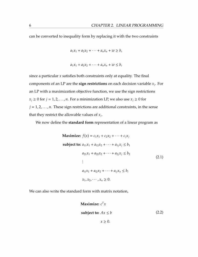
We now define the standard form representation of a linear program as
Maximize: f (x) = c1x1 + c2x2 + · · · + c jx j
subject to: a11x1 + a12x2 + · · · + a1 jx j ≤ b1
a21x1 + a22x2 + · · · + a2 jx j ≤ b2
...
ai1x1 + ai2x2 + · · · + ai jxn ≤ bi
x1, x2, · · · , xn ≥ 0.
(2.1)
We can also write the standard form with matrix notation,
Maximize: cTx
subject to: Ax ≤ b
x ≥ 0.
(2.2)
CHAPTER 2. LINEAR PROGRAMMING 7
where A is an m by n matrix of constraint coefficients ai j, c is a vector of length
n of objective function coefficients, and b is a vector of right-hand side
coefficients of length m.
2.1.2 Solutions
We now consider the solution methods and solution types of LPs. Most
LPs are much too complex to solve by hand or by graphical methods. Instead,
we typically use the Simplex method algorithm. Broadly, the Simplex method
searches the vertices of the feasible region to find the optimal solution. The
mechanics of the Simplex method are not a focus of this project and are well
documented elsewhere, including in [12].
Using the Simplex method, we can find several different types of solutions.
An n-tuple (x1, x2, · · · , xn) specifying a value for each decision variable is a
solution; it is a feasible solution if it satisfies all of the constraints of the LP
and an optimal solution if it corresponds to the actual maximum or minimum
of the LP. The optimal solution is also a feasible solution, by definition. Any
solution that fails to satisfy one or more constraints is an infeasible solution.
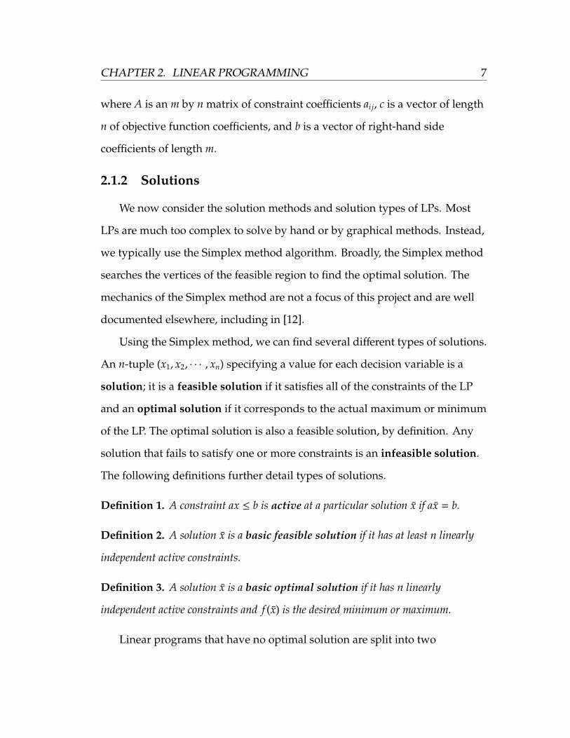
The following definitions further detail types of solutions.
Definition 1. A constraint ax ≤ b is active at a particular solution x̄ if ax̄ = b.
Definition 2. A solution x̄ is a basic feasible solution if it has at least n linearly
independent active constraints.
Definition 3. A solution x̄ is a basic optimal solution if it has n linearly
independent active constraints and f (x̄) is the desired minimum or maximum.
Linear programs that have no optimal solution are split into two
8 CHAPTER 2. LINEAR PROGRAMMING
categories. Some LPs have no feasible solutions; that is, the space defined by
the constraints is empty. For example, consider the LP
Maximize: f (x) = 3x1 + 2x2 + 4x3
subject to: x1 + x2 + x3 ≤ 5
− x1 − x2 − x3 ≤ −8
2x1 + x2 ≤ 10
x1, x2, x3 ≥ 0.
(2.3)
Note that the second constraint can be rewritten as x1 + x2 + x3 ≥ 8. This is
contrary to the first constraint; there is no (x1, x2, x3) that satisfies
x1 + x2 + x3 ≤ 5 and x1 + x2 + x3 ≥ 8. Thus, there are no feasible solutions to this
LP. We call an LP that has no feasible solutions infeasible.
In contrast, some LPs are said to be unbounded. An unbounded LP has
feasible solutions for arbitrarily large objective function values. For example,
consider the LP
Maximize: f (x) = x1 − 6x2
subject to: − 4x1 + x2 ≤ −1
− x1 − 4x2 ≤ −2
x1, x2 ≥ 0.
(2.4)
Let x1 ≥ 2 and x2 = 0; any solution of this form satisfies both constraints and is
feasible. As x1 increases, so does f (x) = x1 − 6x2. Thus, f (x) takes on arbitrarily
large values and is unbounded. We can now categorize the solution categories
CHAPTER 2. LINEAR PROGRAMMING 9
of all linear programs with the following theorem.
Theorem 1. (Fundamental Theorem of Linear Programming) For an arbitrary linear
program in standard form, the following statements are true:
1. If there is no optimal solution, then the problem is either infeasible or unbounded.
2. If a feasible solution exists, then a basic feasible solution exists.
3. If an optimal solution exists, then a basic optimal solution exists.
For more detail and a proof of this theorem, see [12].
2.2 Duality
For many applications of linear programming, it is useful to consider the
dual LP associated with a particular primal LP. These structures come in
pairs; the following section details their relationship. In short, every feasible
solution for one of the programs characterizes a bound on the optimal
objective function value of the other. In fact, both LPs will have the same
optimal objective function value.
2.2.1 Motivation
Before exploring duality theory in general, we offer a motivating example.
Consider the following LP:
Maximize: f (x) = 2x1 + x2 + 3x3
subject to: 3x2 + x3 ≤ 5
x1 + x2 + x3 ≤ 10
3x1 + 2x2 ≤ 8.
(2.5)

10 CHAPTER 2. LINEAR PROGRAMMING
Denote the optimal solution to this LP x∗, and the corresponding optimal
objective function value as f (x∗). Consider a particular feasible solution
(x1, x2, x3) = (2, 0, 5), which has a objective function value of z = 19. In effect,
this z acts as a lower bound for the optimal objective function value z∗. Since
we are attempting to maximize our objective function, the optimal solution
must satsify z∗ ≥ 19. If we cannot find another feasible solution such that this
is true, it must be the case that f (x∗) = 19 and x∗ = (x1, x2, x3) = (2, 0, 5). Thus,
each f (x) acts as a lower bound for the optimal f (x∗).
We can also place upper bounds on f (x∗), as follows. Consider the sum of
the three constraints,
3x2 + x3 ≤ 5
x1 + x2 + x3 ≤ 10
+ 3x1 + 2x2 ≤ 8
4x1 + 6x2 + 2x3 ≤ 23
Since each variable is nonnegative, this sum forms an upper bound on the
optimal objective function value; that is,
2x1 + x2 + 3x3 ≤ 4x1 + 6x2 + 2x3 ≤ 23.
Therefore, we have 19 ≤ f (x∗) ≤ 23. We can find other upper bounds by
considering any linear combination of the constraints of the LP in (2.5).
We have significantly narrowed the range of possible values for f (x∗), but
we can further reduce the size of this interval. Before, we considered a
particular linear combination of the constraint vectors. We now consider a
CHAPTER 2. LINEAR PROGRAMMING 11
linear combination with variables y1, y2, and y3 as the respective constants,
and find these y values that give an upper bound of 0 on f (x). We have
y1(3x2 + x3) ≤ 5y1
y2(x1 + x2 + x3) ≤ 10y2
+ y3(3x1 + 2x2) ≤ 8y3
(y2 + 3y3)x1 + (3y1 + y2 + 2y3)x2 + (y1 + y2)x3 ≤ 5y1 + 10y2 + 8y3
Assume that each of the xi coefficients is the same as in the original objective
function. That is,
y2 + 3y3 ≥ 2
3y1 + y2 + 2y3 ≥ 1
y1 + y2 ≥ 3.
(2.6)
Thus,
f (x) = 2x1 + x2 + 3x3
≤ (y2 + 3y3)x1 + (3y1 + y2 + 2y3)x2 + (y1 + y2)x3
≤ 5y1 + 10y2 + 8y3.
Since f (x) is bounded above by 5y1 + 10y2 + 8y3, we can minimize this sum in
order to find the most specific upper bound for the original LP. This new
12 CHAPTER 2. LINEAR PROGRAMMING
objective function is constrained by (2.6), and we naturally have the dual LP
Minimize: g(y) = 5y1 + 10y2 + 8y3
subject to: y2 + 3y3 ≥ 2
3y1 + y2 + 2y3 ≥ 1
y1 + y2 ≥ 3.
(2.7)
This is the dual LP associated with the given primal LP (2.5). Intuitively, the
dual LP seeks to minimize (maximize) the upper (lower) bound on the primal
objective function, respectively.
2.2.2 Theory
We now present the formal theory of duality, emphasizing the relationship
between primal-dual LP pairs and their respective solutions. We also consider
the relationship between various solution types and the dual LP.
Definition 4. For a primal LP in the standard form of
Maximize:n∑
j=1
c jx j
subject to:n∑
j=1
ai jx j ≤ bi 1 ≤ i ≤ m
x j ≥ 0 1 ≤ j ≤ n
(2.8)
CHAPTER 2. LINEAR PROGRAMMING 13
the corresponding dual LP is given by
Minimize:m∑
i=1
biyi
subject to:m∑
i=1
yiai j ≥ c j 1 ≤ j ≤ n
yi ≥ 0 1 ≤ i ≤ m.
(2.9)
Proposition 1. The dual of a dual LP is the primal LP.
Proof. To verify this relationship, we must first write the dual problem in
standard form. Recall that a standard form LP maximizes its objective
function and has ≤ constraints. The sign restrictions remain the same. Since
minimizing a function is equivalent to maximizing its negative, we have
minm∑
i=1
biyi = −max
m∑i=1
biyi
We can convert the ≥ constraints to ≤ by multiplying both sides by -1. Thus,
the standard form of the dual LP is given by
Maximize:m∑
i=1
biyi
subject to:m∑
i=1
−yiai j ≤ −c j 1 ≤ j ≤ n
yi ≥ 0 1 ≤ i ≤ m.
14 CHAPTER 2. LINEAR PROGRAMMING
The dual of this LP is
Minimize:n∑
j=1
−c jx j
subject to:n∑
j=1
(−ai j)x j ≥ −bi 1 ≤ i ≤ m
x j ≥ 0 1 ≤ j ≤ n,
which is equivalent to the primal LP given by
Maximize:n∑
j=1
c jx j
subject to:n∑
j=1
ai jx j ≤ bi 1 ≤ i ≤ m
x j ≥ 0 1 ≤ j ≤ n.
�
We can also characterize the relationship between the feasible solutions of
the primal and dual LPs.
Theorem 2. [12] Weak Duality Theorem: If (x1, x2, · · · , xn) is a feasible solution for
the primal LP and (y1, y2, · · · , yn) is feasible for the associated dual LP, then∑j c jx j ≤
∑i biyi.
CHAPTER 2. LINEAR PROGRAMMING 15
Proof. We have the following series of inequalities
∑j
c jx j ≤
∑j
∑i
yiai j
x j
=∑
i j
yiai jx j
=∑
i
∑j
ai jx j
yi
≤
∑i
biyi.
(2.10)
For the first inequality, we know that each x j ≥ 0 by (2.8) that c j ≤∑
i yiai j for
each j by (2.9). The second inequality is similar; yi ≥ 0 by (2.9) and∑
j ai jx j ≤ bi
by (2.8) for each i. �
From the Weak Duality Theorem, we know that all of the primal objective
function values (for feasible solutions) are less than all of the dual objective
function values. For an arbitrary primal feasible solution x, f (x) ≤ g(y) for all
dual feasible solutions y, where f and g are the primal and dual objective
functions, respectively. This provides an upper bound for every primal
objective function value. Similarly, the objective function value for any primal
optimal solution provides a lower bound for every dual objective function
value. Therefore, we can characterize the optimal solutions x and y as those
for which f (x) = g(y).
We now have the necessary background to draw a connection between the
optimal solutions of a primal-dual LP pair. We present the following theorem
without proof, as the particular mechanics are outside the scope of this project.
16 CHAPTER 2. LINEAR PROGRAMMING
For more detail, see [12]. Intuitively, this theorem states that the objective
functions for a primal-dual pair of LPs is equal precisely at the optimal
solution to each.
Theorem 3. [12] Strong Duality Theorem: For an optimal solution x∗ ∈ Rn to a
primal LP, there is a dual LP which has an optimal solution y∗ ∈ Rn such that∑j c jx∗j =
∑i biy∗i .
Chapter 3
Game Theory
This chapter presents several concepts in game theory that are central to
this project. We focus on the various representations and types of games, as
well as the associated Nash equilibria. These concepts will later be used in
conjunction with the linear programming theory of the previous chapter to
develop a method of representing and solving two variants of poker.
3.1 Background
The purpose of game theory is to develop mathematical models that
represent decision-making interactions among individuals. We assume that
these individuals are both rational in their own decisions and take into
account expectations of how the other decision-makers will act [7]. Game
theory can be used to model a wide range of situations, including business
negotiations, political competition, and economic models of oligopolistic
competition, as well as traditional ‘games‘, such as chess, checkers, and poker.
Game theoretic models are highly abstracted versions of the actual situation.
17
18 CHAPTER 3. GAME THEORY
Unlike many other fields of mathematics, the study of game theory attempts to
both positively describe how individuals do make decisions, and normatively
how they should under the assumption of perfect rationality.
The modern field of game theory is relatively new, and is generally
considered to have begun in the 19th century with Cournot, Bertrand, and
Edgeworth’s respective work on models of oligopoly pricing [4]. These ideas
developed to a more general theory of games in the mid-19th century with
John von Neumann’s proof of the existence of mixed-strategy equilibria in
two-person zero-sum games. He later co-authored the seminal Theory of Games
and Economic Behavior with Oskar Morgenstern [4]. This text considered
theoretical results about cooperative games with several players, and offered a
axiomatic conception of utility theory that allowed mathematicians to
formalize decision-making under uncertainty. Additionally, it introduced the
concepts of the normal (or strategic) and extensive forms, as well as a proof of
the existence of a maximin equilibrium for all two-player zero-sum games [4].
With zero-sum games fairly well understood, attention turned to the more
general case of non zero-sum games, which are perhaps more common. In
1950, John Forbes Nash Jr. proved the existence of an optimal strategy for each
player in every non-cooperative game [4]. The Nash equilibrium is a
generalization of Morgenstern’s maximin theorem for non zero-sum games,
and requires that each player’s optimal strategy be a payoff-maximizing
response to his correct expectation of his opponents strategy. This guarantee
was a significant advance in the field, and allowed the study of a broader class
of games [4].
CHAPTER 3. GAME THEORY 19
3.2 Normal (Strategic) Form
One of the most common representations of a game is the normal form,
also known as the strategic form. Intuitively, it represents a game as a payoff
matrix with each player’s (pure) strategies as particular rows and columns.
The payoffs to each player are determined by their respective strategies. The
normal form is the typical representation for small 2-player games with
simultaneous decision making, but can be extended to larger games and those
that initially appear to have non-simultaneous decision making. The concepts
in this section are based heavily on [7]. We begin with the formal definition of
a normal form game.
Definition 5. A game in normal (strategic) form is a tuple⟨N, (Ai), (%i)
⟩, with
• a finite set of N players
• for each player i ∈ N, the nonempty set of available actions Ai
• a set of action profiles a = (a j) for j ∈ N, where each a j corresponds to a
particular action in A j
• for each player i ∈ N, a preference relation %i on A1 × A2 × . . . × A j for j ∈ N
Any such game with a finite set of actions Ai for each player i is considered finite.
Notice that the preferences of each player i are defined over A, instead of
Ai; that is, their preferences are defined over each combination of the other
player’s outcomes, as well as their own. This distinguishes a strategic game
from a more general decision problem; players are concerned with their
20 CHAPTER 3. GAME THEORY
opponents actions and payoffs, as well as their own. The normal form model
of a game is intentionally abstract, allowing it to be applied to a wide variety
of situations. The set of players N may consist of individuals, animals,
governments, businesses, etc. Likewise, the set of actions Ai may contain only
a few simple actions or complicated sets of contingencies over many potential
outcomes. The primary restriction on the elements of N and each A is that
each player has a well-defined preference relation over all outcomes of action
profile combinations. For example, the preference relation for a business
might be a function that maps particular actions to profit levels.
This definition considers a generalized preference relation %i; typically, and
for our purposes, we can use a more intuitive payoff function ui. In this case,
we denote a particular game as⟨N, (Ai), (ui)
⟩. This payoff function ui maps a
particular combination of action profiles to a numerical payoff value. These
inputs can be represented either as a singular action profile a ∈ A or as a tuple
to highlight the actions of individual players. For example, a particular u1(a)
represents the payoff to player 1 for a particular combination of each player’s
actions a ∈ A. This action profile a defines a particular action a j for each player
j from their action set A j. Alternatively, we may wish to highlight particular
action profiles from distinct players as separate inputs to ui. Players typically
wish to choose a set of actions that maximize this value, wish could represent
profit, utility, etc. The utility function describes how a particular player feels
about a particular combination of actions of all of the players in the game.
Definition 6. For a game with a set of outcomes A = A1 × A2 × . . . × A j for j ∈ N,
the function ui : A 7→ R is the payoff function with ui(a) ≥ ui(b) whenever a %i b for
CHAPTER 3. GAME THEORY 21
combinations of actions a, b ∈ A.
In a game, players make choices about how they will play. Each of these
choices is a particular action take by a player at some point in the game. In a
game with more than one such set of action choices, players employ a
strategy, which is an algorithmic prescription of every action that a player will
choose. A particular strategy could be a simple choice between two actions, or
a complicated set of prescriptions to choose actions based on various
contingencies of how the other players act. These choices may or may not be
identical across iterations of the game, motivating the following distinction.
Definition 7. A pure strategy si is a deterministic prescription of how an individual
will play a game, choosing the same action at every iteration. A strategy set Si is the
set of all pure strategies available to player i. A mixed strategy σi assigns a
probability to each pure strategy.
The probabilities assigned to each pure strategy s in a mixed strategy σ are
governed by a global probability distribution. For example, let S1 = (s1, s2, s3)
represent the strategy set of player 1 with pure strategies s1, s2, and s3 in some
strategic game. A particular mixed strategy σ = (0.4, 0.1, 0.5) represents player
1 employing each pure strategy with the respective probabilities.
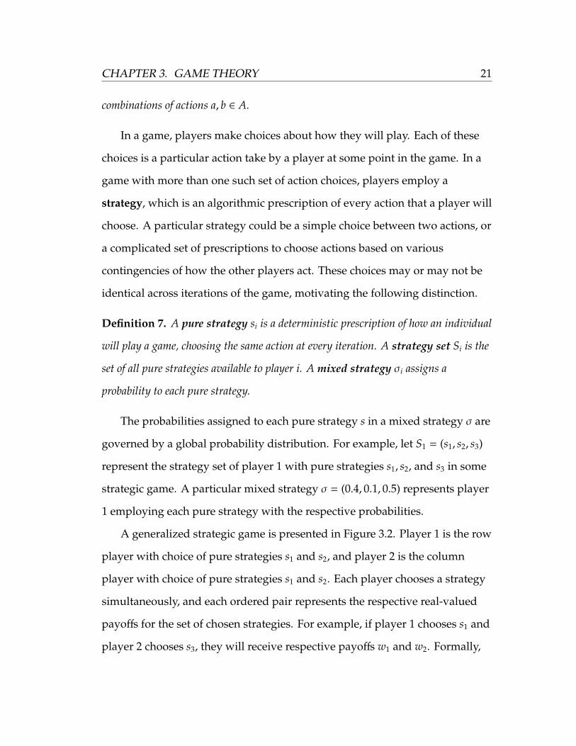
A generalized strategic game is presented in Figure 3.2. Player 1 is the row
player with choice of pure strategies s1 and s2, and player 2 is the column
player with choice of pure strategies s1 and s2. Each player chooses a strategy
simultaneously, and each ordered pair represents the respective real-valued
payoffs for the set of chosen strategies. For example, if player 1 chooses s1 and
player 2 chooses s3, they will receive respective payoffs w1 and w2. Formally,
22 CHAPTER 3. GAME THEORY
u1(s1, s3) = w1 and u2(s1, s3) = w2.
p2
s3 s4
p1s1 (w1,w2) (x1, x2)s2 (y1, y2) (z1, z2)
Figure 3.1: Generalized Two-player Strategic Game
However, each player need not always play the same strategy in this
game. It may be necessary to vary their play in order to optimize their
expected payoff. This is the motivation behind the concept of a mixed strategy.
Recall that a mixed strategy σi is a probability distribution over all of player i’s
pure strategies. The probabilities assigned to each pure strategy determine the
expected payoff of the mixed strategy. For example, consider a particular
mixed strategy σ1 in which player 1 chooses s1 with probability 0.7 and s2 with
probability 0.3. Player 2 uses mixed strategy σ2 , where he chooses s3 and s4
with equal probability. Then the payoff to player 1 is
u1(σ1, σ2) = 0.7(0.5w1+0.5x1)+0.3(0.5y1+0.5z1) = 0.35w1+0.35x1+0.15y1+0.15z1.
(3.1)
More generally, the payoff for a mixed strategy profile is a linear function
of the probabilities assigned to each pure strategy [4]. In (3.1), the coefficient
associated with a particular payoff value is the product of the probabilities
assigned to the particular pure strategy of each player in their mixed strategy.
Player 1 uses pure strategy s1 with probability 0.7 in his mixed strategy σ1, and
player 2 uses pure strategy s3 with probability 0.3 in his mixed strategy σ2. In
this case, player 1’s payoff is w1. This occurs with probability 0.7 × 0.5 = 0.35.
CHAPTER 3. GAME THEORY 23
Therefore, the overall expected value to player 1 for this σ1, σ2 combination is
a weighted sum of the payoffs to each combination of pure strategies.
3.2.1 Equilibrium
In any game, each player tries to maximize their own payoff. Payoffs are
dependent on the combination of strategies that each employs. Thus, the
decision of which strategy to employ is critical. This section begins by
considering the Nash equilibrium of any normal form game, and then
considers the more specific case of Maximin equilibrium in strictly competitive
games. Both refer to a steady state wherein each player correctly assumes how
the other(s) will play and chooses his own strategy rationally in response.
Generally, a game is said to be in equilibrium if no player can improve their
payoff by unilaterally changing strategy.
Nash Equilibria
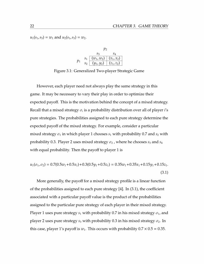
The concept of the Nash equilibrium is well illustrated through the classic
example of the Prisoner’s Dilemma, as shown through a normal form
representation in Figure 3.2. This is a standard example in game theory
literature, and illustrates several important concepts. The rules of the game are
as follows: Two individuals are arrested by the police, and are suspected of
committing a crime together. The police lack sufficient evidence to convict
either on the most serious charge, but enough to convict either on a less
serious charge. Each individual is offered a choice: betray the other and testify
to the police that the other committed the most serious crime, or stay silent
and accept the conviction of the lesser charge. If both betray each other, the
24 CHAPTER 3. GAME THEORY
penalty is reduced by one year for each. The individuals cannot communicate
with each other as they decide whether or not to betray their co-conspirator.
Unsurprisingly, they each want to minimize the number of years that they
spend in prison. The potential payoffs, in years in prison respectively, are
shown in Figure 3.2.
p2
Betray Silent
p1Betray (3, 3) (0, 4)Silent (4, 0) (1, 1)
Figure 3.2: Prisoner’s Dilemma
We can determine each player’s best strategy by considering the potential
payoffs of each of their choices, along with the other player’s choices. Each
player chooses if they want to confess. If the row player stays silent, he will
serve 3 years in prison if the column player also stays silent, or he will walk
free if the column player confesses. Conversely, if the row player does confess,
he will serve 4 years or 1 year, respectively. In either case the dominant
strategy is for the row player to confess, since he will receive less prison time
in each contingency of the column player’s choice. We can repeat this analysis
for the column player, and find that his dominant strategy is also to confess. If
both players choose rationally and consider what the other may do, they will
both choose to confess. This is the Nash equilibrium of the Prisoner’s
Dilemma.
With this intuitive understanding, we can now formalize this logic and
develop the theory more generally. This section focuses on the Nash
equilibrium of the normal form representation; the concept extends naturally
CHAPTER 3. GAME THEORY 25
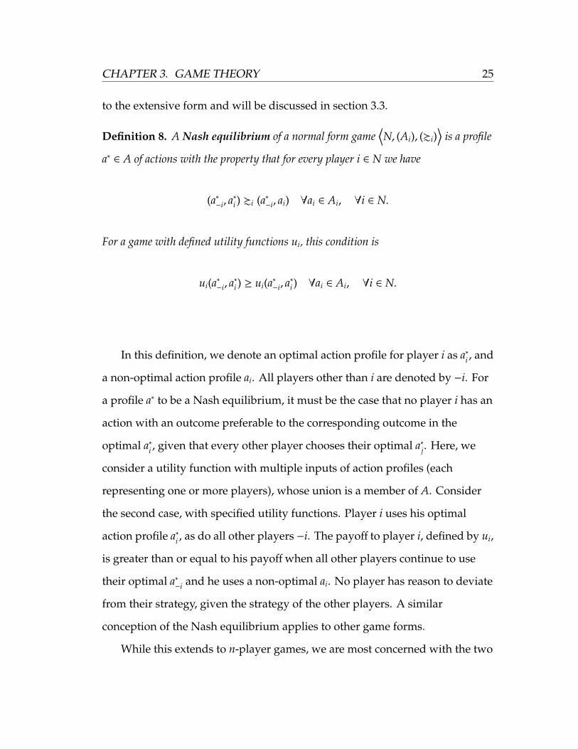
to the extensive form and will be discussed in section 3.3.
Definition 8. A Nash equilibrium of a normal form game⟨N, (Ai), (%i)
⟩is a profile
a∗ ∈ A of actions with the property that for every player i ∈ N we have
(a∗−i, a
∗
i ) %i (a∗−i, ai) ∀ai ∈ Ai, ∀i ∈ N.
For a game with defined utility functions ui, this condition is
ui(a∗−i, a∗
i ) ≥ ui(a∗−i, a∗
i ) ∀ai ∈ Ai, ∀i ∈ N.
In this definition, we denote an optimal action profile for player i as a∗i , and
a non-optimal action profile ai. All players other than i are denoted by −i. For
a profile a∗ to be a Nash equilibrium, it must be the case that no player i has an
action with an outcome preferable to the corresponding outcome in the
optimal a∗i , given that every other player chooses their optimal a∗j. Here, we
consider a utility function with multiple inputs of action profiles (each
representing one or more players), whose union is a member of A. Consider
the second case, with specified utility functions. Player i uses his optimal
action profile a∗i , as do all other players −i. The payoff to player i, defined by ui,
is greater than or equal to his payoff when all other players continue to use
their optimal a∗−i and he uses a non-optimal ai. No player has reason to deviate
from their strategy, given the strategy of the other players. A similar
conception of the Nash equilibrium applies to other game forms.
While this extends to n-player games, we are most concerned with the two
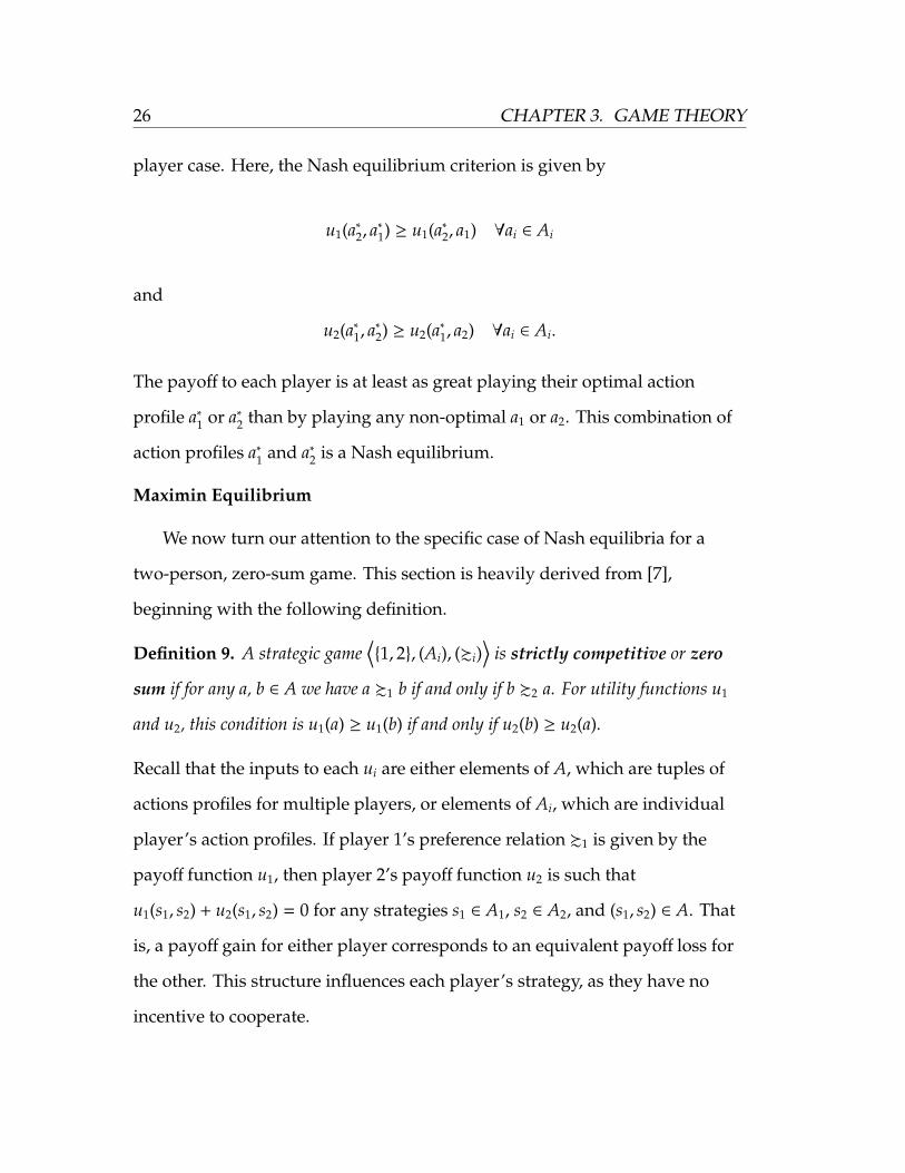
26 CHAPTER 3. GAME THEORY
player case. Here, the Nash equilibrium criterion is given by
u1(a∗2, a∗
1) ≥ u1(a∗2, a1) ∀ai ∈ Ai
and
u2(a∗1, a∗
2) ≥ u2(a∗1, a2) ∀ai ∈ Ai.
The payoff to each player is at least as great playing their optimal action
profile a∗1 or a∗2 than by playing any non-optimal a1 or a2. This combination of
action profiles a∗1 and a∗2 is a Nash equilibrium.
Maximin Equilibrium
We now turn our attention to the specific case of Nash equilibria for a
two-person, zero-sum game. This section is heavily derived from [7],
beginning with the following definition.
Definition 9. A strategic game⟨{1, 2}, (Ai), (%i)
⟩is strictly competitive or zero
sum if for any a, b ∈ A we have a %1 b if and only if b %2 a. For utility functions u1
and u2, this condition is u1(a) ≥ u1(b) if and only if u2(b) ≥ u2(a).
Recall that the inputs to each ui are either elements of A, which are tuples of
actions profiles for multiple players, or elements of Ai, which are individual
player’s action profiles. If player 1’s preference relation %1 is given by the
payoff function u1, then player 2’s payoff function u2 is such that
u1(s1, s2) + u2(s1, s2) = 0 for any strategies s1 ∈ A1, s2 ∈ A2, and (s1, s2) ∈ A. That
is, a payoff gain for either player corresponds to an equivalent payoff loss for
the other. This structure influences each player’s strategy, as they have no
incentive to cooperate.
CHAPTER 3. GAME THEORY 27
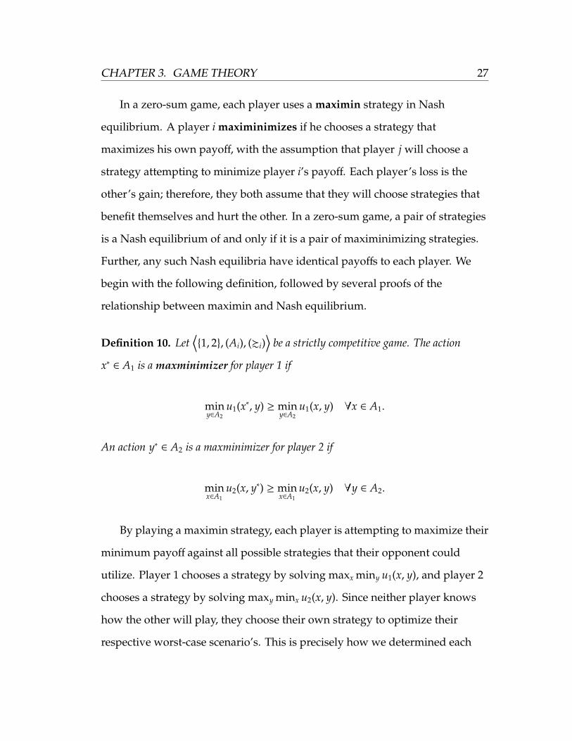
In a zero-sum game, each player uses a maximin strategy in Nash
equilibrium. A player i maximinimizes if he chooses a strategy that
maximizes his own payoff, with the assumption that player j will choose a
strategy attempting to minimize player i’s payoff. Each player’s loss is the
other’s gain; therefore, they both assume that they will choose strategies that
benefit themselves and hurt the other. In a zero-sum game, a pair of strategies
is a Nash equilibrium of and only if it is a pair of maximinimizing strategies.
Further, any such Nash equilibria have identical payoffs to each player. We
begin with the following definition, followed by several proofs of the
relationship between maximin and Nash equilibrium.
Definition 10. Let⟨{1, 2}, (Ai), (%i)
⟩be a strictly competitive game. The action
x∗ ∈ A1 is a maxminimizer for player 1 if
miny∈A2
u1(x∗, y) ≥ miny∈A2
u1(x, y) ∀x ∈ A1.
An action y∗ ∈ A2 is a maxminimizer for player 2 if
minx∈A1
u2(x, y∗) ≥ minx∈A1
u2(x, y) ∀y ∈ A2.
By playing a maximin strategy, each player is attempting to maximize their
minimum payoff against all possible strategies that their opponent could
utilize. Player 1 chooses a strategy by solving maxx miny u1(x, y), and player 2
chooses a strategy by solving maxy minx u2(x, y). Since neither player knows
how the other will play, they choose their own strategy to optimize their
respective worst-case scenario’s. This is precisely how we determined each
28 CHAPTER 3. GAME THEORY
player’s optimal strategy in the Prisoner’s Dilemma (Figure 3.2).
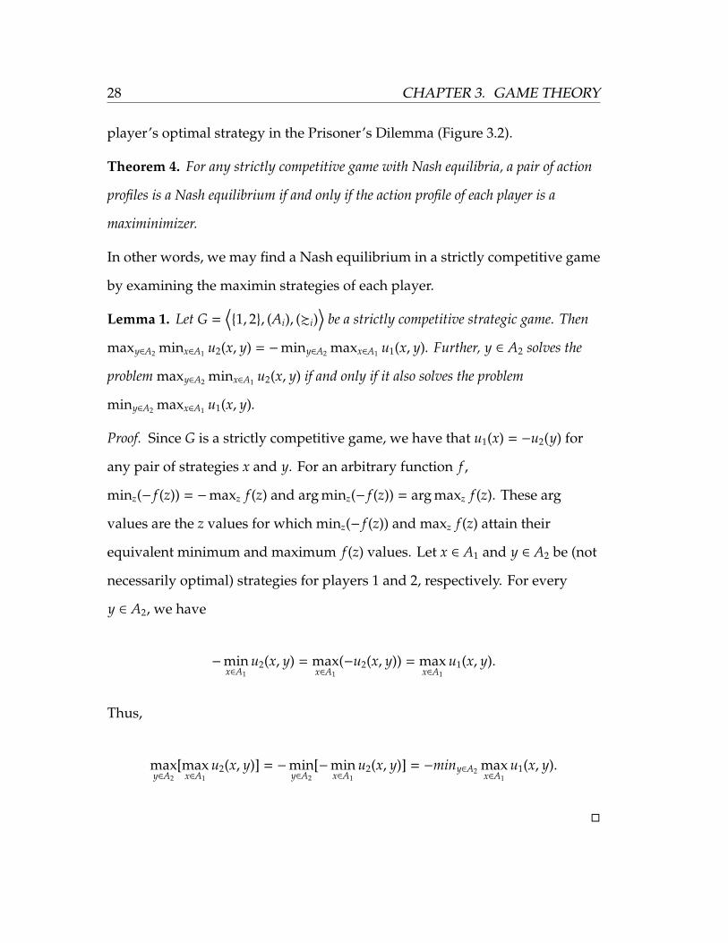
Theorem 4. For any strictly competitive game with Nash equilibria, a pair of action
profiles is a Nash equilibrium if and only if the action profile of each player is a
maximinimizer.
In other words, we may find a Nash equilibrium in a strictly competitive game
by examining the maximin strategies of each player.
Lemma 1. Let G =⟨{1, 2}, (Ai), (%i)
⟩be a strictly competitive strategic game. Then
maxy∈A2 minx∈A1 u2(x, y) = −miny∈A2 maxx∈A1 u1(x, y). Further, y ∈ A2 solves the
problem maxy∈A2 minx∈A1 u2(x, y) if and only if it also solves the problem
miny∈A2 maxx∈A1 u1(x, y).
Proof. Since G is a strictly competitive game, we have that u1(x) = −u2(y) for
any pair of strategies x and y. For an arbitrary function f ,
minz(− f (z)) = −maxz f (z) and arg minz(− f (z)) = arg maxz f (z). These arg
values are the z values for which minz(− f (z)) and maxz f (z) attain their
equivalent minimum and maximum f (z) values. Let x ∈ A1 and y ∈ A2 be (not
necessarily optimal) strategies for players 1 and 2, respectively. For every
y ∈ A2, we have
−minx∈A1
u2(x, y) = maxx∈A1
(−u2(x, y)) = maxx∈A1
u1(x, y).
Thus,
maxy∈A2
[maxx∈A1
u2(x, y)] = −miny∈A2
[−minx∈A1
u2(x, y)] = −miny∈A2 maxx∈A1
u1(x, y).
�
CHAPTER 3. GAME THEORY 29
Proposition 2. Let G =⟨{1, 2}, (Ai), (%i)
⟩be a strictly competitive game.
(a) If (x∗, y∗) is a Nash equilibrium of G then x∗ is a maximin strategy for player 1
and y∗ is a maximin strategy for player 2.
(b) If (x∗, y∗) is a Nash equilibrium of G, then
maxx miny u1(x, y) = miny maxx u1(x, y) = u1(x∗, y∗), and all Nash equilibria
of G yield identical payoffs.
(c) If x∗ and y∗ are maximin strategies for player’s 1 and 2 respectively, then (x∗, y∗)
is a Nash equilibrium of G.
Proof. We first prove (a) and (b) in conjunction. Let (x∗, y∗) be a Nash
equilibrium of G. Then u2(x∗, y∗) ≥ u2(x∗, y) for all y ∈ A2. Likewise, since
u2 = −u1, u1(x∗, y∗) ≤ u1(x∗, y) for all y ∈ A2. Therefore,
u1(x∗, y∗) = miny u1(x∗, y) ≤ maxx miny u1(x, y). Similarly, u1(x∗, y∗) ≥ u1(x, y∗) for
all x ∈ A1. Therefore, u1(x∗, y∗) ≥ miny u1(x, y) for all x ∈ A1, so that
u1(x∗, y∗) ≥ maxx miny u1(x, y). Therefore, u1(x∗, y∗) = maxx miny u1(x, y) and x∗
is a maximin strategy for player 1. An analogous argument shows that y∗ is a
maximin strategy for player 2 and that u2(x∗, y∗) = maxy minx(x, y), so that
u1(x∗, y∗) = miny maxx u1(x, y).
For part (c), let v∗ = maxx miny u1(x, y) = miny maxx u1(x, y). From Lemma
1, we know that maxy minx u2(x, y) = −v∗. Since x∗ is a maximin strategy for
player 1, we have u1(x∗, y) ≥ −v∗ for all y ∈ A2. Likewise, since y∗ is a maximin
strategy for player 2, we have u2(x, y∗) ≥ −v∗ for all x ∈ A2. Setting y = y∗ and
30 CHAPTER 3. GAME THEORY
x = x∗, we have u1(x∗, y∗) = v∗. Since u2 = −u1, we conclude that (x∗, y∗) is a
Nash equilibrium of G.
�
A crucial implication of part (c) is that a Nash equilibrium can be found by
solving the problem maxx miny u1(x, y). For a strictly competitive game, the
Nash-optimal strategy is precisely the solution to the maximin problem. If
maxx miny u1(x, y) = miny maxx u1(x, y), we define this equilibrium payoff to
player 1 as the value of the game. From Proposition 2, we know that if v∗ is the
value of a strictly competitive game, then any equilibrium strategy gives a
payoff to player 1 of at least v∗ and to player 2 at least −v∗ [7].
3.3 Extensive Form
A second representation of many games is the extensive form. The
extensive form represents a game as a directed graph that maps all possible
moves and outcomes. The extensive form best represents sequential games of
non-simultaneous decision-making. It is particularly amenable to imperfect
information games, such as poker, where some information about the game
state is hidden from each player. The following section details the theory of
the extensive form, including a discussion of the associated Nash equilibrium.
We also distinguish between the extensive form games with perfect and
imperfect information. This section closely follows [7].
3.3.1 Perfect Information
Definition 11. An extensive form game with perfect information is represented
by the tuple⟨N,H,P,%i
⟩, where:
CHAPTER 3. GAME THEORY 31
• A finite set N (the set of players)
• A set H of sequences (finite or infinite) that satisfies the following three
properties:
– The empty sequence ∅ is a member of H.
– If (ak)k=1,...,K ∈ H (where K may be infinite) and L < K then (ak)k=1,··· ,L ∈ H.
– If an infinite sequence (ak)k=1,··· satisfies (ak)k=1,··· ,L ∈ H for every positive
integer L then (ak)k=1,··· ∈ H.
• Each member of H is a history; each component of a history is an action taken
by a player. A history (ak)k=1,··· ,K ∈ H is terminal if it is infinite or if there is no
ak+1 such that (ak)k=1,··· ,k+1 ∈ H. The set of terminal histories is denoted Z.
• A function P that assigns to each nonterminal history (each member of H \ Z) a
member of N ∪ {c}. This P is the player function, P(h) being the player who
takes an action after the history h. If P(h) = c, then chance determines the action
taken after the history h.
• For each player i ∈ N, a preference relation %i on Z.
Let h be a history of length k; the ordered pair (h, a) is the history of length
k + 1 consisting of h followed by a. For any non-terminal history h, the player
function P(h) chooses an action a from the set
A(h) = {a : (h, a) ∈ H}.
At the beginning of any extensive game, this history is empty; no actions have
previously occurred. For the empty sequence ∅ ∈ H, the player P(∅) chooses a
32 CHAPTER 3. GAME THEORY
member of A(∅). Each member of A(∅) is an action a0. For each of these
choices, the player defined by P(a0) chooses a member of the set A(a0). For
each possible choice in A(a0), denoted a1, player P(a1) chooses a member of the
set A(a1). This process iterates until the game reaches a terminal history.
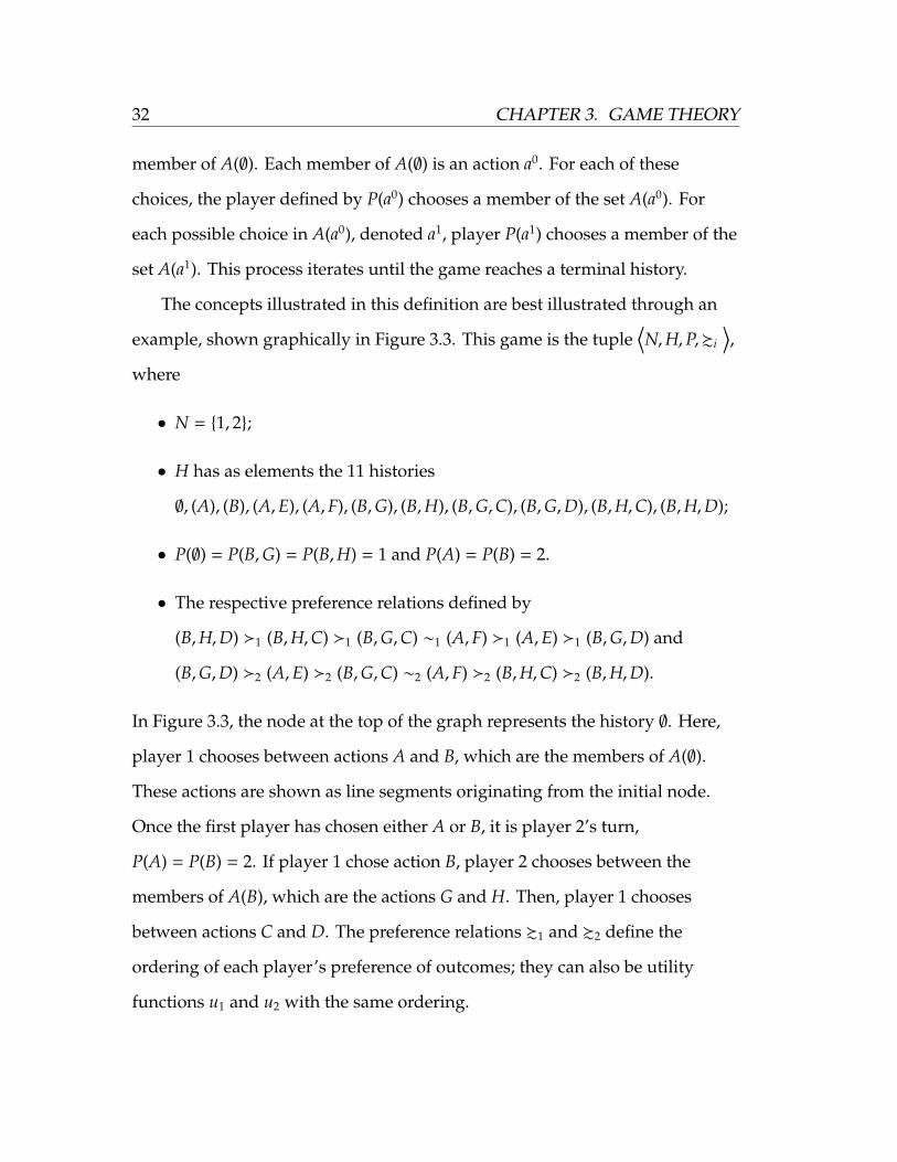
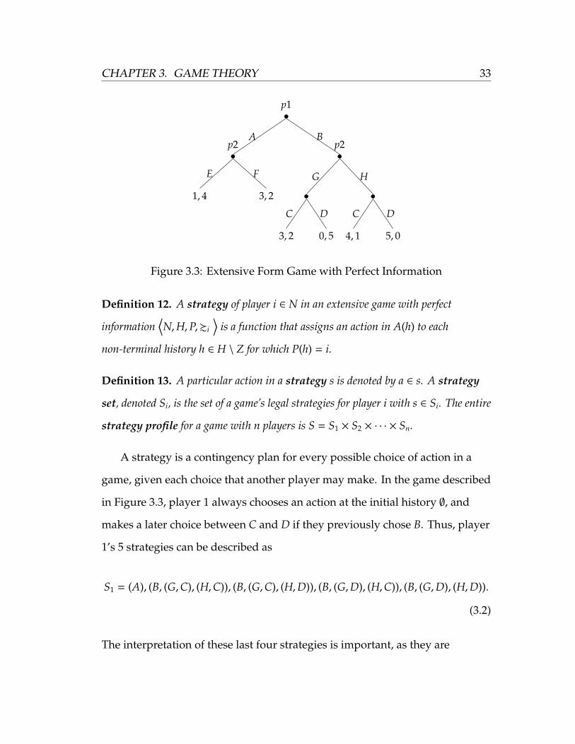
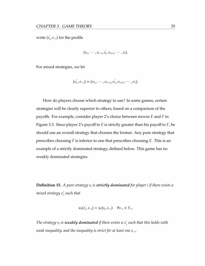
The concepts illustrated in this definition are best illustrated through an
example, shown graphically in Figure 3.3. This game is the tuple⟨N,H,P,%i
⟩,
where
• N = {1, 2};
• H has as elements the 11 histories
∅, (A), (B), (A,E), (A,F), (B,G), (B,H), (B,G,C), (B,G,D), (B,H,C), (B,H,D);
• P(∅) = P(B,G) = P(B,H) = 1 and P(A) = P(B) = 2.
• The respective preference relations defined by
(B,H,D) �1 (B,H,C) �1 (B,G,C) ∼1 (A,F) �1 (A,E) �1 (B,G,D) and
(B,G,D) �2 (A,E) �2 (B,G,C) ∼2 (A,F) �2 (B,H,C) �2 (B,H,D).
In Figure 3.3, the node at the top of the graph represents the history ∅. Here,
player 1 chooses between actions A and B, which are the members of A(∅).
These actions are shown as line segments originating from the initial node.
Once the first player has chosen either A or B, it is player 2’s turn,
P(A) = P(B) = 2. If player 1 chose action B, player 2 chooses between the
members of A(B), which are the actions G and H. Then, player 1 chooses
between actions C and D. The preference relations %1 and %2 define the
ordering of each player’s preference of outcomes; they can also be utility
functions u1 and u2 with the same ordering.
CHAPTER 3. GAME THEORY 33
p1
p2
1, 4
E
3, 2
F
Ap2
3, 2
C
0, 5
D
G
4, 1
C
5, 0
D
H
B
Figure 3.3: Extensive Form Game with Perfect Information
Definition 12. A strategy of player i ∈ N in an extensive game with perfect
information⟨N,H,P,%i
⟩is a function that assigns an action in A(h) to each
non-terminal history h ∈ H \ Z for which P(h) = i.
Definition 13. A particular action in a strategy s is denoted by a ∈ s. A strategy
set, denoted Si, is the set of a game’s legal strategies for player i with s ∈ Si. The entire
strategy profile for a game with n players is S = S1 × S2 × · · · × Sn.
A strategy is a contingency plan for every possible choice of action in a
game, given each choice that another player may make. In the game described
in Figure 3.3, player 1 always chooses an action at the initial history ∅, and
makes a later choice between C and D if they previously chose B. Thus, player
1’s 5 strategies can be described as
S1 = (A), (B, (G,C), (H,C)), (B, (G,C), (H,D)), (B, (G,D), (H,C)), (B, (G,D), (H,D)).
(3.2)
The interpretation of these last four strategies is important, as they are
34 CHAPTER 3. GAME THEORY
contingent on player 2’s actions. For example, the strategy (B, (G,C), (H,D))
represents the following contingency plan: after first choosing action B, if
player 2 chooses G, take action C. Otherwise, if player 2 takes action H, player
1 chooses D. Player 2’s strategies are simpler, and can be described as
S2 = ((A,E), (B,G)), ((A,E), (B,H)), ((A,F), (B,G)), ((A,F), (B,H)). (3.3)
The strategy ((A,E), (B,G)) is interpreted as follows: if player 1 chooses A,
choose E. Otherwise, if player 1 chooses B, choose G.
It is important to note that a particular strategy defines the action to be
chosen for each history, even if that history is never reached when the strategy
is employed. For example, consider the strategy (A, (G,C), (H,C)) for player 1.
If he chooses action A, the later choice between C and D cannot happen.
Despite this, we still specify what player 1 would do in that scenario. In this
way, a formal strategy in an extensive game differs from an intuitive plan of
action.
Definition 14. A pure strategy si of player i ∈ N in an extensive game⟨N,H,P,%i)
⟩is a deterministic prescription of how to play a game. A mixed strategy σi is a
probability distribution over all pure strategies.
This concepts of pure and mixed strategies is similar to that in the normal
form representation. For the game in Figure 3.3, (3.2) and (3.3) are the pure
strategies. We use the following notation to distinguish between the pure and
mixed strategies of the various players in any game. We often consider the
strategy of a particular player i, while holding the strategies of his opponents
fixed. Let s−i ∈ S−i denote the strategy selection for all other players than i, and
CHAPTER 3. GAME THEORY 35
write (s′i , s−i) for the profile
(s1, · · · , si−1, s′
i , si+1, · · · , si).
For mixed strategies, we let
(σ′
i , σ−i) = (σ1, · · · , σi−1, σ′
i , σi+1, · · · , σi).
How do players choose which strategy to use? In some games, certain
strategies will be clearly superior to others, based on a comparison of the
payoffs. For example, consider player 2’s choice between moves E and F in
Figure 3.3. Since player 2’s payoff to E is strictly greater than his payoff to F, he
should use an overall strategy that chooses the former. Any pure strategy that
prescribes choosing F is inferior to one that prescribes choosing E. This is an
example of a strictly dominated strategy, defined below. This game has no
weakly dominated strategies.
Definition 15. A pure strategy si is strictly dominated for player i if there exists a
mixed strategy σ′i such that
ui(σ′
i , s−i) > ui(si, s−i) ∀s−i ∈ S−i
The strategy si is weakly dominated if there exists a σ′i such that this holds with
weak inequality, and the inequality is strict for at least one s−i.
36 CHAPTER 3. GAME THEORY
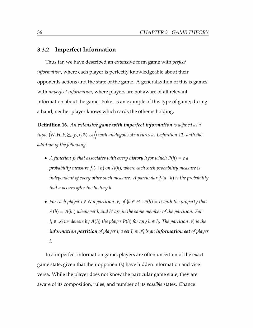
3.3.2 Imperfect Information
Thus far, we have described an extensive form game with perfect
information, where each player is perfectly knowledgeable about their
opponents actions and the state of the game. A generalization of this is games
with imperfect information, where players are not aware of all relevant
information about the game. Poker is an example of this type of game; during
a hand, neither player knows which cards the other is holding.
Definition 16. An extensive game with imperfect information is defined as a
tuple⟨N,H,P,%i, fc, (Ii)i∈N)
⟩with analogous structures as Definition 11, with the
addition of the following
• A function fc that associates with every history h for which P(h) = c a
probability measure fc(· | h) on A(h), where each such probability measure is
independent of every other such measure. A particular fc(a | h) is the probability
that a occurs after the history h.
• For each player i ∈ N a partition Ii of {h ∈ H : P(h) = i} with the property that
A(h) = A(h′) whenever h and h′ are in the same member of the partition. For
Ii ∈ Ii we denote by A(Ii) the player P(h) for any h ∈ Ii. The partition Ii is the
information partition of player i; a set Ii ∈ Ii is an information set of player
i.
In a imperfect information game, players are often uncertain of the exact
game state, given that their opponent(s) have hidden information and vice
versa. While the player does not know the particular game state, they are
aware of its composition, rules, and number of its possible states. Chance
CHAPTER 3. GAME THEORY 37
determines the particular game state. The “Chance player“ c is represented by
fc, which defines a probability measure for each history h such that P(h) = c.
For example, consider a card game in which two players hold one of three
cards with none repeated. Since there are 6 possible combinations of cards,
fc(a | h) = 16 for the relevant history h. This probability is uniform across each
deal, defining a complete probability distribution.
The final key structures in an imperfect information game are the
information partitions Ii and information sets Ii. Each player i has a singular
Ii that partitions the set of histories H into information sets Ii. An information
set describes all of the histories that are identical from the point of view of a
particular player. Of course, these histories are not actually identical; they
differ only in the hidden information. Two histories h and h′ are in the same
information set only if A(h) = A(h′). That is, the set of actions available for the
two histories is identical. Notice that this implies the known information is
identical for all elements of an information set; the player cannot distinguish
between them.
Definition 17. An extensive form game has perfect recall if for each player i we have
Xi(h) = Xi(h′) wherever the histories h and h′ are in the same information set of player
i.
In a game with perfect recall, no player forgets information that they knew
at a previous state. This information includes previous actions and any hidden
information known only to that player, as well as previous information sets.
Later information sets must refine previous information sets from earlier
histories. If this is not the case, then the game has imperfect recall. It is not
38 CHAPTER 3. GAME THEORY
necessary that an extensive form game with imperfect information have
perfect recall; some have imperfect recall. However, the variants of poker
examined in later sections are both games of perfect recall.
p1
p2
p1
−1, 1
l
1,−1
r
O
p1
3,−3
l
−2, 2
r
P
M
p2
p1
0, 0
L
1,−1
R
O
p1
1,−1
L
3,−3
R
P
N
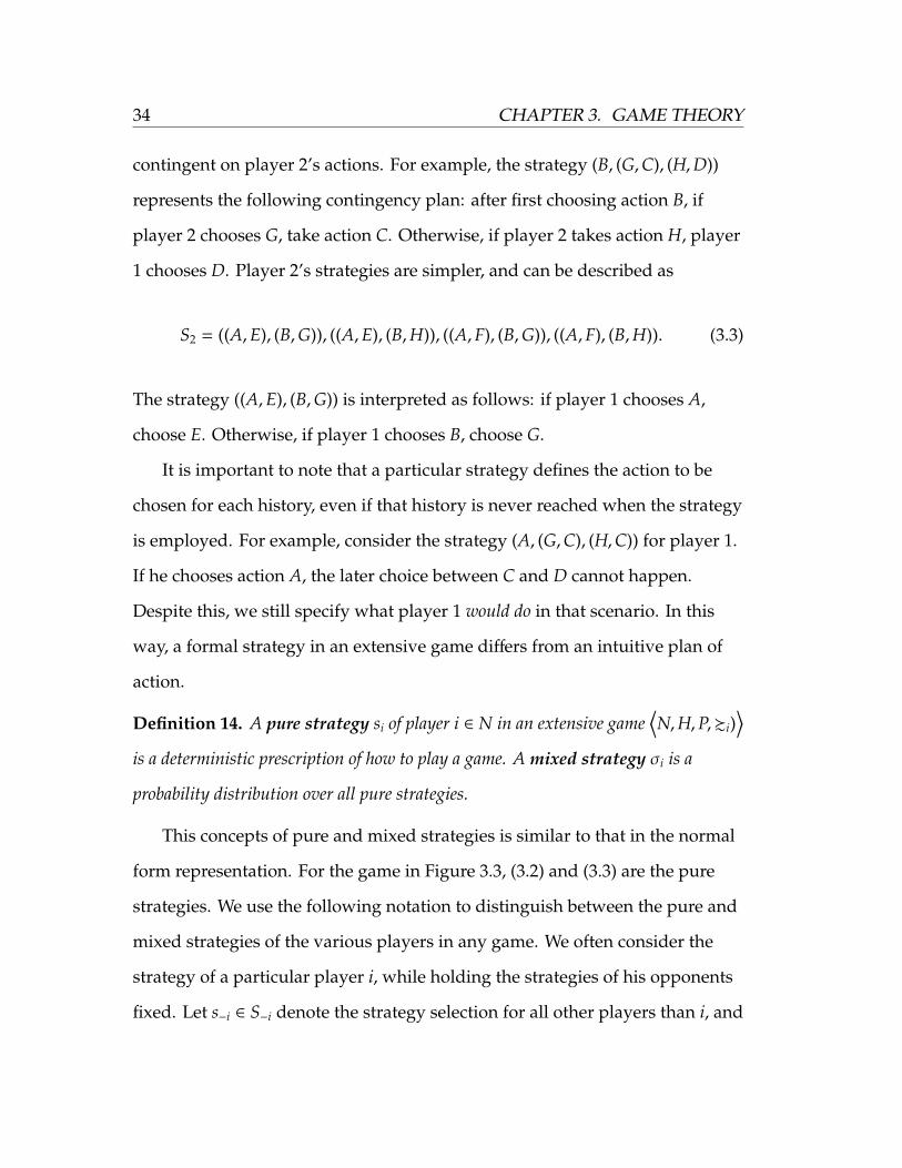
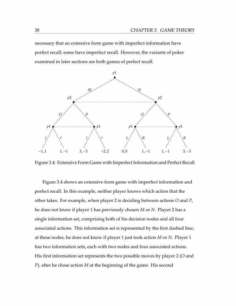
Figure 3.4: Extensive Form Game with Imperfect Information and Perfect Recall
Figure 3.4 shows an extensive form game with imperfect information and
perfect recall. In this example, neither player knows which action that the
other takes. For example, when player 2 is deciding between actions O and P,
he does not know if player 1 has previously chosen M or N. Player 2 has a
single information set, comprising both of his decision nodes and all four
associated actions. This information set is represented by the first dashed line;
at these nodes, he does not know if player 1 just took action M or N. Player 1
has two information sets, each with two nodes and four associated actions.
His first information set represents the two possible moves by player 2 (O and
P), after he chose action M at the beginning of the game. His second
CHAPTER 3. GAME THEORY 39
information set contains the two game states possible after he chose action N
originally. Notice that these player 1’s information sets refine previous
distinctions; there is one set where he previously took action M, and another
where he took action N. Further, notice that player 1’s possible actions are
identical across all nodes in an information set, but are also unique to that
information set. He faces the choice between l and r only when he previously
chose M, and between L and R only when he previously chose N.
Definition 18. A pure strategy of player i ∈ N in an extensive game with imperfect
information⟨N,H,P,%i, fc, (Ii)i∈N)
⟩is a function that assigns an action in A(Ii) to
each information set Ii ∈ Ii.
Definition 19. A mixed strategy of player i in an extensive game with imperfect
information⟨N,H,P,%i, fc, (Ii)i∈N)
⟩is a probability measure over the set of player i’s
pure strategies. A behavioral strategy of player i is a collection (βi(Ii))Ii∈Ii of
independent probability measures, where βi(Ii) is a probability measure over A(Ii).
For any history h ∈ Ii ∈ Ii and action a ∈ A(h) we denote by βi(h)(a) the
probability βi(Ii)(a) assigned by βi(Ii) to the action a. That is, βi(Ii)(a) is the
probability that player i will choose action a information set Ii. The collection
of these probabilities, for each possible action within each information set,
defines a behavioral strategy. This distinction between a mixed strategy and a
behavioral strategy illustrates two ways in which a player may choose to
randomize their behavior. A mixed strategy uses a probability distribution
over all possible pure strategies, whereas a behavioral strategy uses separate
probability distribution for each information set. The resulting randomized
strategy appears identical to an observer of the game, and may be outcome
40 CHAPTER 3. GAME THEORY
equivalent.
Definition 20. Let σ = (σi)i∈N be a profile of mixed or behavioral strategies for an
extensive game with imperfect information. The outcome O(σ) of σ is the probability
distribution over the terminal histories that results when each player i follows the
strategy specification of σi.
Definition 21. Two strategies, either mixed or behavioral, are outcome equivalent
if for every collection of pure strategies of the other players the two strategies induce
the same outcome.
Proposition 3. For any mixed strategy of a player in a finite extensive game with
perfect recall, there is an outcome-equivalent behavioral strategy.
3.3.3 Nash Equilibrium
We now present a brief theory of the Nash equilibrium for extensive form
games with imperfect information.
Definition 22. A Nash equilibrium in mixed strategies of an extensive game is a
profile σ∗ of mixed strategies with the property that for every player i ∈ N we have
O(σ∗−i, σ
∗
i ) %i O(σ∗−i, σi)
for every mixed strategy σi of player i. A Nash equilibrium in behavioral
strategies is defined analogously.
This version of the Nash equilibrium is very similar to that of the normal form
and the extensive form perfect information case. The optimal mixed strategy
CHAPTER 3. GAME THEORY 41
σ∗i has a more preferable outcome O than any non-optimal strategy σi. No
player can benefit by unilaterally changing his strategy. In a mixed strategy
Nash equilibrium, we have a probability distribution over each possible pure
strategy. In a behavioral strategy Nash equilibrium, we have a probability
distribution over the actions in each information set. The following lemma is
implied by Proposition 3.
Lemma 2. For an extensive game with perfect recall, the Nash equilibria in mixed
and behavioral strategies are equivalent.
3.4 Sequence Form
The final game representation that we consider is the sequence form,
which is related to the extensive form. The extensive form describes a
imperfect information game, specifying its information sets, actions, payoffs,
etc. While the graphical representation allows the reader to quickly
understand the mechanics of the game well, it does not allow for efficient
computation of an optimal strategy. Typically, an extensive form game must be
converted to normal form, and a maximin LP algorithm considers all possible
pure strategies of the game. For an example of this process, see Section 4.3.
The number of pure strategies is exponential in the size of the game tree; this
often makes efficient computation of an optimal strategy infeasible [13].
The purpose of the sequence form is to overcome this disadvantage, and
allow the efficient computation of an optimal strategy. It is represented as a
matrix scheme, similar to the normal form. However, the pure strategies from
the normal form are replaced with sequences of consecutive moves. Instead of
42 CHAPTER 3. GAME THEORY
computing the probabilities assigned to each pure strategy, we consider the
realization probabilities of these sequences actually being played. These
realization probabilities can be used to construct a behavior strategy, which
describes the probability distribution over each information set. These optimal
behavior strategies can be found using an LP algorithm; each player’s optimal
behavior strategy is an optimal solution to the primal and dual LPs,
respectively. This section develops the theory of the sequence form, based on
the original development in [13].
Many of the structures of the sequence form are similar to those in the
extensive form. Recall that an extensive form game has a chance player and N
personal players. The chance player governs the chance node(s) by one or
more probability distributions, and the personal players govern the decision
nodes by their prescribed strategy. The sequence form defines a strategy
differently; instead of defining a probability distribution over all pure
strategies or over each information set, the player considers each payoff node
of the game tree and the sequence of actions necessary to get there. These
sequences are the basic unit of analysis in this form.
Definition 23. A sequence s of choices of player i defined by a node a of the game
tree, is the set of actions in H on the path from the root node to a. The set of sequences
of player i is denoted Si.
We now denote s as a sequence, instead of a strategy as in previous
sections. It is clear from context which is being used. A sequence is defined by
the particular set of action labels that a player takes on his path to some node
a. In a game with perfect recall, members of a particular information set must
CHAPTER 3. GAME THEORY 43
have identical histories; thus, a sequence can be defined completely in terms of
the actions made to arrive at the given node. The set of all sequences Si
replaces the set of pure strategies Si in the normal form. We also consider the
sequences of the chance player 0, where each chance node has an associated
probability distribution. Payoffs are defined by combinations of sequences,
including those of the chance player and all personal players.
Definition 24. Let h(a) be a function that maps each terminal node a to a payoff
vector in Rn. The payoff function g : S0 × S1 × · · · × Sn 7→ RN is defined by
g(s) = h(a) if s is the (N + 1)-tuple (s0, s1, · · · , sN) of sequences defined by a leaf a of
the game tree, and by g(s) = (0, · · · , 0) ∈ RN otherwise. Note that the chance player
sequence s∅ occurs with probability 1 and will always be the first input in g.
The tuple (s0, s1, . . . , sN) is unique for a particular node a in the game tree;
therefore, the payoff function g is well defined. The number of sequences is at
most the number of nodes, which grows linearly with the size of the game
tree. In contrast, the number of pure strategies in the normal form grows
exponentially, since each pure strategy must consider each combination of
actions at all possible information sets. For a two-player game with a known
chance player, the matrix P is the payoff matrix with each of player 1 and 2’s
sequences as the rows and columns, respectively. A particular entry Pi j is the
payoff of sequences si and s j being played by the two respective personal
players; that is, Pi j = g(s∅, si, s j). Many combinations of sequences between the
two players are impossible; they define combinations of actions that cannot
occur in conjunction with each other. Thus, the number of non-zero entries in
A is at most the number of leaves in the game tree. All other entries are 0, since
44 CHAPTER 3. GAME THEORY
they have no defined payoff.
We must also consider how particular sequences are chosen by a player.
For a normal form game, players can use either a pure or mixed strategy; both
define a choice of action in every possible contingency of the game. In the
sequence form, the player must define a probability distribution for each
information set. This distribution determines the frequency of choosing each
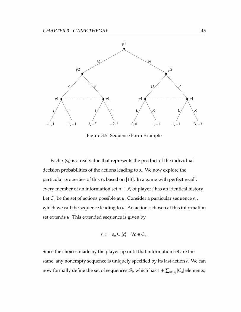
action, with its associated sequence. For example, consider Figure 3.5; this
game is identical to Figure 3.4, but with player 1’s initial action known to
player 2. Note that player 2 can now distinguish between his two decision
nodes, and that the actions stemming from each are now unique. Player 2
must choose between sequences o and p if player 1 chooses M, as well as O and
P if player 1 chooses N. For example, he may always choose o when player 1
choose M, and always P when player 1 chooses N. This is the pure strategy
(o,P). In terms of sequences, this corresponds to assigning probabilities
(1, 1, 0, 0, 1) to his sequences (s∅, so, sp, sO, sP). Instead of mixed strategy
probabilities, the sequence form uses the realization probabilities of sequences
when the player uses a behavior strategy. Intuitively, the realization plan for a
particular sequence is a product of individual decision probabilities of the
actions c necessary to reach that sequence.
Definition 25. The realization plan of βi is a function ri : Si 7→ R defined as
ri(si) =∏c∈si
βi(c),
where c is an action in a sequence si. This ri follows (3.4), (3.5), and (3.6).
CHAPTER 3. GAME THEORY 45
p1
p2
p1
−1, 1
l
1,−1
r
o
p1
3,−3
l
−2, 2
r
p
M
p2
p1
0, 0
L
1,−1
R
O
p1
1,−1
L
3,−3
R
P
N
Figure 3.5: Sequence Form Example
Each ri(si) is a real value that represents the product of the individual
decision probabilities of the actions leading to si. We now explore the
particular properties of this ri, based on [13]. In a game with perfect recall,
every member of an information set u ∈ Ii of player i has an identical history.
Let Cu be the set of actions possible at u. Consider a particular sequence su,
which we call the sequence leading to u. An action c chosen at this information
set extends u. This extended sequence is given by
suc = su ∪ {c} ∀c ∈ Cu.
Since the choices made by the player up until that information set are the
same, any nonempty sequence is uniquely specified by its last action c. We can
now formally define the set of sequences Si, which has 1 +∑
u∈Ii|Cu| elements;
46 CHAPTER 3. GAME THEORY
one for each action in each information set, and one for the empty sequence s∅.
Each elemenet in Si is a particular sequence s. Notice that the number of
sequences in a game is at most the number of terminal (payoff) nodes; an LP
that considers individual sequences will typically have fewer variables than
an LP that considers all possible pure strategies.
Definition 26. The set of sequences Si is defined as Si = {∅} ∪ {suc | u ∈ Ii, c ∈ Cu}.
In order to account for the non-terminal decision nodes, the realization
plan ri has the following constraints. The initialization of the game,
represented by the empty sequence s∅, has probability 1. Every game has
exactly one of these sequences. That is,
ri(s∅) = 1 (3.4)
Since each behavior strategy is a probability distribution over an information
set, we know that∑
c∈Cuβi(c) = 1. Therefore, the realization probability of a
sequence must equal the sum of the realization probabilities for that sequence
extended over all of its possible extending actions c. We can think of the
probability of reaching a particular sequence as being “distributed” over all of
these extending actions. Formally,
−ri(su) +∑c∈Cu
ri(suc) = 0 ∀u ∈ Ii ∀su ∈ Si. (3.5)
Finally, realization probabilities are non-negative:
ri(si) ≥ 0 ∀si ∈ Si. (3.6)
CHAPTER 3. GAME THEORY 47
The following proposition links a realization plan with a behavior strategy.
Recall that a behavior strategy, as opposed to a mixed strategy, defines a
probability distribution over all of the actions in each information set.
Proposition 4. Any realization plan arises from a suitable behavior strategy.
Proof. Consider a realization plan ri with associated behavior strategy βi, and
an arbitrary information set u ∈ Ii. Define the behavior at u by
βi(c) =ri(suc)ri(su)
∀c ∈ Cu
if ri(su) > 0 and arbitrarily such that
∑c∈Cu
βi(c) = 1
if ri(su) = 0. By induction on the length of a sequence, we have Definition 25 by
definition. Thus, any realization plan arises from a suitable behavior
strategy. �
Definition 27. Any information set u for which ri(su) = 0 in behavior strategy βi is
called irrelevant.
A behavior strategy does not prescribe any action over an irrelevant
information set because it will never be reached, given earlier prescriptions of
the behavior strategy. This will be an important point in Chapters 4 and 5; the
sequence form linear programming algorithms output initially surprising
results for some information sets. These particular values will be irrelevant, as
those information sets cannot be realized under the optimal behavioral
48 CHAPTER 3. GAME THEORY
strategy.
Mixed strategies can also be represented by a realization plan. Recall that a
mixed strategy is a combination of pure strategies with probabilities assigned
to each. This mixed strategy has a corresponding set of realization plans that
follow Definition 25. However, information is lost in converting a mixed
strategy to a realization plan, since the later does not need to cover every
possible contingency of the game. It only must cover the sequences and
information sets that the player will actually need to choose from with their
behavior strategy. Fortunately, the realization plan does retain the strategically
relevant aspects.
Definition 28. A set of mixed strategies are realization equivalent if for any fixed
strategies (pure or mixed) of the other players, all of the mixed strategies define the
same probabilities for reaching the nodes of the game tree.
Proposition 5. Mixed strategies are realization equivalent if and only if they have the
same realization plan.
Corollary 1. For a player with perfect recall, any mixed strategy is realization
equivalent to a behavior strategy.
Thus, a realization plan corresponds to a behavior strategy, which in turn
corresponds to a mixed strategy. By defining a realization plan for each player,
we are essentially describing a mixed strategy.
3.4.1 Linear Programming Theory
We now define the necessary linear programming theory to find the
optimal strategy for a two-player zero-sum extensive game with perfect recall,
CHAPTER 3. GAME THEORY 49
based on [13]. This game is first converted to sequence form using the theory
of the previous section. The sequence form structures are used to build a
primal-dual pair of LPs. We want to find a pair of realization plans, which can
be converted into behavior strategies. The components of an optimal
realization plan are probability distributions over each information set. The
sequence form translates to a primal-dual pair of LPs, whose solutions are the
optimal realization plans for each player.
This section uses the following notation. The realization plans r1 and r2 are
denoted as column vectors x and y which have |S1| and |S2| entries,
respectively. The constraint matrices E and F show that x and y are valid
realization plans in accordance with Definition (25), with Ex = e and Fy = f .
Here, E and F have |S1| and |S2| columns, respectively. They have 1 + |I1| and
1 + |I2| rows, respectively. Both e and f are unit vectors of the appropriate
dimension. The payoff matrix P has |S1| rows and |S2| columns, and individual
payoff entries are calculated according to Definition (24). The payoffs are with
respect to player 1; in this zero-sum game, player 2’s expected payoffs are
given by −P. The expected payoff to realization plans x and y are xTPy and
−xTPy for the respective players.
We first consider an LP to find the best response y of player 2 to a fixed
realization plan x of player 1. If player 1 plays according to x, then player 2’s
best response is the optimal solution to the LP
Maximize: f (y) = −(xTP)y
subject to: Fy = y
y ≥ 0.
(3.7)
50 CHAPTER 3. GAME THEORY
In this LP, player 2 wants to utilize a realization plan y that maximizes his
payoff given by −(xTP)y. This realization plan must correspond to a legal set
of moves, giving the constraint Fy = y. Finally, since each element of y is a
probability, we have y ≥ 0. We also have the dual of this LP, given by
Minimize: f (q) = qT f
subject to: qTF ≥ −xTP.(3.8)
The dual variables are given by the vector q, which has 1 + |I2| elements.
We have an analogous pair of LP’s for the best response x of player 1 given
realization plan y for player 2. This finds a realization plan x that maximizes
player 1’s payoff xT(Py). This x must satisfy the constraints xTET = eT and x ≥ 0
that define a valid realization plan. The primal is
Maximize: f (x) = xT(Py)
subject to: xTET = eT
x ≥ 0.
(3.9)
The dual problem uses the unconstrained vector p, which has 1 + |I2|
elements. It is given by
Minimize: f (p) = eTp
subject to: ETp ≥ Py.(3.10)
These LPs describe algorithms for finding the optimal realization plans of
one player, given a particular realization plan of the other. We require an LP
CHAPTER 3. GAME THEORY 51
that generates the Nash equilibrium strategies, in which each player actively
considers the other’s strategy. Consider that (3.7) and (3.10) have the same
optimal objective function value; that is xT(Ay) = eTp. This is the payoff to
player 1, given that player 2 uses realization plan y. If y is not fixed and can be
varied by player 2, he will try to minimize this payoff. Since this is a zero-sum
game, player 2 wants to minimize any payoff he gives to player 1, as this will
maximize his own payoff. If we consider that y can vary, it must be subject to
the same constraints as (3.9). Thus, player 1’s optimal strategy is the solution
to the following LP:
Minimize: f (y, p) = eTp
subject to: − Py + ETp ≥ 0
Fy = f
y ≥ 0.
(3.11)
Player 2’s optimal strategy is the solution to the dual LP, given by
Maximize: f (x, q) − qT f
subject to: xT(−P) − qTF ≤ 0
xTET = eT
x ≥ 0.
(3.12)
Theorem 5. The equilibria of a zero sum game with perfect recall are the optimal
primal and dual solutions of this sequence form linear program whose size, in sparse
representation, is linear in the size of the game tree.
52 CHAPTER 3. GAME THEORY
Proof. Consider the primal LP in (3.11) with optimal solution y, p and the dual
LP in (3.12) with optimal solution x, q. Based on previous discussion, the
number of nonzero entries of the payoff matrix P and of the constraint
matrices E and F grows linearly with the game tree. By definition, y and p are
feasible solutions to (3.7) and (3.8), respectively. Likewise, x and q are feasible
solutions to (3.9) and (3.10). Multiplying the Fy = f constraint in (3.7) by qT
and the constraint in (3.8) gives
qT f = qTFy ≤ −xTPy. (3.13)
For player 1, the same process yields
eTp = xETp ≥ xTPy. (3.14)
We can combine these expressions as
eTp ≥ xTPy ≥ −qT f . (3.15)
The inequality in (3.13) is the Weak Duality Theorem (2). The value of the
objective function xTPy from (3.7) is bounded from above by its dual objective
function value qT f from (3.8). Analogously, (3.14) shows this bound for the
primal-dual pair of (3.9) and (3.8) and (3.15) for (3.11) and (3.12). Recall the
Strong Duality Theorem (3), which states that a pair of primal/dual solutions
are optimal only if the associated objective functions are equal. Applying this
to (3.11) and (3.12), we have that eTp = −qT f . This implies that equality holds
in (3.13), (3.14), and (3.15). Thus, x is an optimal solution to (3.9) and a best
CHAPTER 3. GAME THEORY 53
response to y, and vice versa. Therefore, x and y represent an equilibrium.
For the dual LP, any equilibrium x and y are solutions to (3.7) and (3.9).
Then, equality analogously holds in (3.13), (3.14), and (3.15), implying that
(3.11) and (3.12) are solved optimally.
�

54 CHAPTER 3. GAME THEORY

Chapter 4
Kuhn Poker
In this chapter, we consider the simple game of Kuhn Poker [5].
Developed in 1950 by Harold W. Kuhn as an example of a two-person
zero-sum imperfect information game, it is an appropriate starting point in
our study of general Nash-optimal poker strategy. We present a graphic
version of the extensive form, as well solutions using linear programming
methods for both the normal and sequence forms.
4.1 Rules
In Kuhn Poker, there are two players and a deck containing the cards Jack,
Queen, and King. No card is repeated. First, each player antes one unit. Each
player is then dealt one card, and the player with the highest card wins the pot
at showdown, provided neither player has folded. After the random deal, the
subsequent betting structure of Kuhn poker is as follows. Player 1 can choose
to either bet one unit or check. If player 1 bets, player 2 has the option of
calling the bet or folding. If player 1 checks, player 2 can either bet one unit or
55
56 CHAPTER 4. KUHN POKER
check. If player 2 bets, player 1 can either call or fold. At this point, if neither
has folded, the hand goes to showdown and the player with the highest card
wins the total pot [5].
4.2 Extensive Form
Figure 4.1 shows the complete extensive form for Kuhn poker. For more
information on the extensive form generally, see Section 3.3. Each node
represents a history, and each edge is an available action that progresses the
game to a new history. The leaves at the bottom of the tree specify the payoff
to player 1 of that particular set of actions and dealt cards. Since this is a
zero-sum game, the payoff to player 2 is simply the negative of player 1’s
payoff. For each edge lower than the results of the deal, a move to the left
represents a check or fold and a move to the right represents a bet or call,
depending on the situation. Each letter adjacent to an edge labels a sequence
and each pair of node colors describes a sample information set, both
described in Section 4.4. In contrast to the normal and sequence forms in the
following sections, the extensive form depiction does not directly translate to a
linear program. This background on the extensive form was found in [1].
4.3 Normal Form
In addition to the extensive form representation of Kuhn poker, we can
also describe its normal form representation. The theory of the normal form
and the associated linear program in this section are modeled on [1]. The
normal form shows the payoffs of particular combinations of each player’s
strategy as an entry of a matrix. We first consider all possible strategy
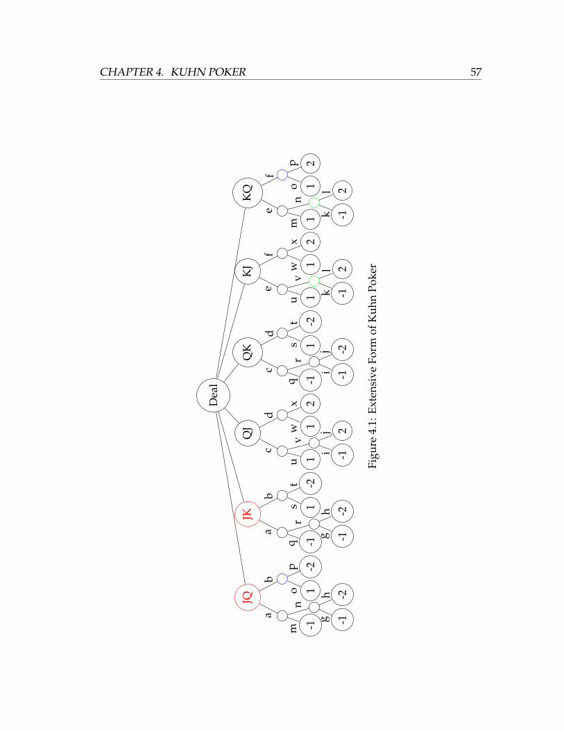
CHAPTER 4. KUHN POKER 57
Dea
l
JQ
-1 -1-21
-2
JK
-1 -1-21
-2
QJ
1 -121
2
QK
-1 -1-21
-2
KJ
1 -121
2
KQ
1 -121
2
a
mn
gh
b
op
a
qr
gh
b
st
c
uv
ij
d
wx
c
qr
ij
d
st
e
uv
kl
f
wx
e
mn
kl
f
op
Figu
re4.
1:Ex
tens
ive
Form
ofK
uhn
Poke
r
58 CHAPTER 4. KUHN POKER
combinations for each player and particular dealing of the three cards.
4.3.1 Strategies
Recall that a pure strategy s in a normal form game is a deterministic
prescription of the strategy set used by a player in a game. A mixed strategy σ
is a strategy that assigns a probability to each pure strategy. A pure strategy as
a special case of mixed strategy, with all but one strategy having probability
zero. A player using a pure strategy would play a game the same way every
time, while a player using a mixed strategy would vary their strategy
randomly with known distribution. For example, in Kuhn Poker, a (poor) pure
strategy would be to always bet as player 1. A mixed strategy would be to
always bet while holding a Jack or King, while betting with a Queen half of the
time.
Each entry in Figure 4.2 represents a complete pure strategy that player 1
could choose, covering all deals and both betting rounds. The prescribed pure
strategy for each held card (J, Q, K) is read from the left, and the comma
delineates player 1’s first round betting strategy from his second round betting
strategy. A P represents a check or fold , B represents a bet or call, and O
represents a non-existent move option in player 1’s second betting round.
Player 1 will use the pass P to fold if player 2 has just bet, and to check if
player 2 has not just bet. For example, PPB, PPO represents player 1 betting
only while holding a King in the first round, and folding all hands if player 2
bets. If player 2 chooses not to bet after we check, the hand goes to showdown;
in this case, the second half of the strategy above is irrelevant. Note that there
is no prescribed strategy (O) for having a King in the second round after
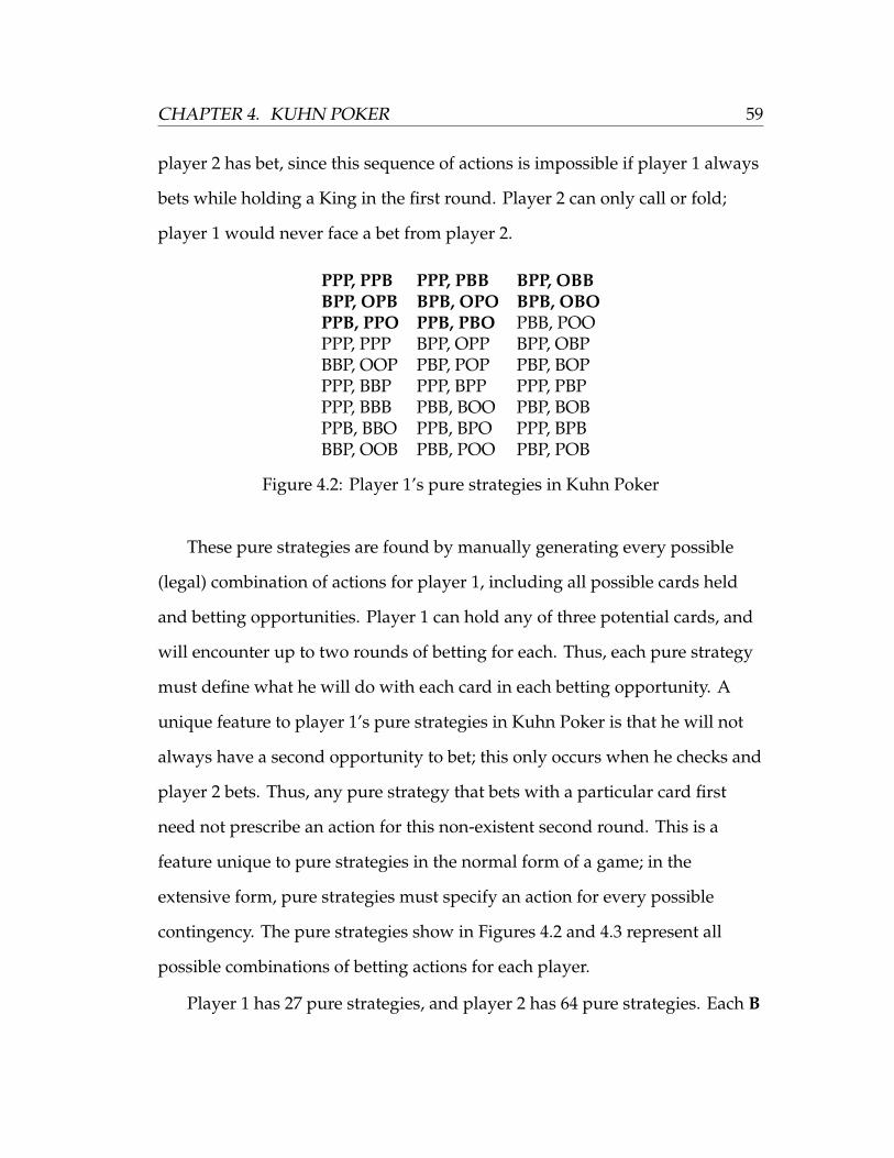
CHAPTER 4. KUHN POKER 59
player 2 has bet, since this sequence of actions is impossible if player 1 always
bets while holding a King in the first round. Player 2 can only call or fold;
player 1 would never face a bet from player 2.
PPP, PPB PPP, PBB BPP, OBBBPP, OPB BPB, OPO BPB, OBOPPB, PPO PPB, PBO PBB, POOPPP, PPP BPP, OPP BPP, OBPBBP, OOP PBP, POP PBP, BOPPPP, BBP PPP, BPP PPP, PBPPPP, BBB PBB, BOO PBP, BOBPPB, BBO PPB, BPO PPP, BPBBBP, OOB PBB, POO PBP, POB
Figure 4.2: Player 1’s pure strategies in Kuhn Poker
These pure strategies are found by manually generating every possible
(legal) combination of actions for player 1, including all possible cards held
and betting opportunities. Player 1 can hold any of three potential cards, and
will encounter up to two rounds of betting for each. Thus, each pure strategy
must define what he will do with each card in each betting opportunity. A
unique feature to player 1’s pure strategies in Kuhn Poker is that he will not
always have a second opportunity to bet; this only occurs when he checks and
player 2 bets. Thus, any pure strategy that bets with a particular card first
need not prescribe an action for this non-existent second round. This is a
feature unique to pure strategies in the normal form of a game; in the
extensive form, pure strategies must specify an action for every possible
contingency. The pure strategies show in Figures 4.2 and 4.3 represent all
possible combinations of betting actions for each player.
Player 1 has 27 pure strategies, and player 2 has 64 pure strategies. Each B
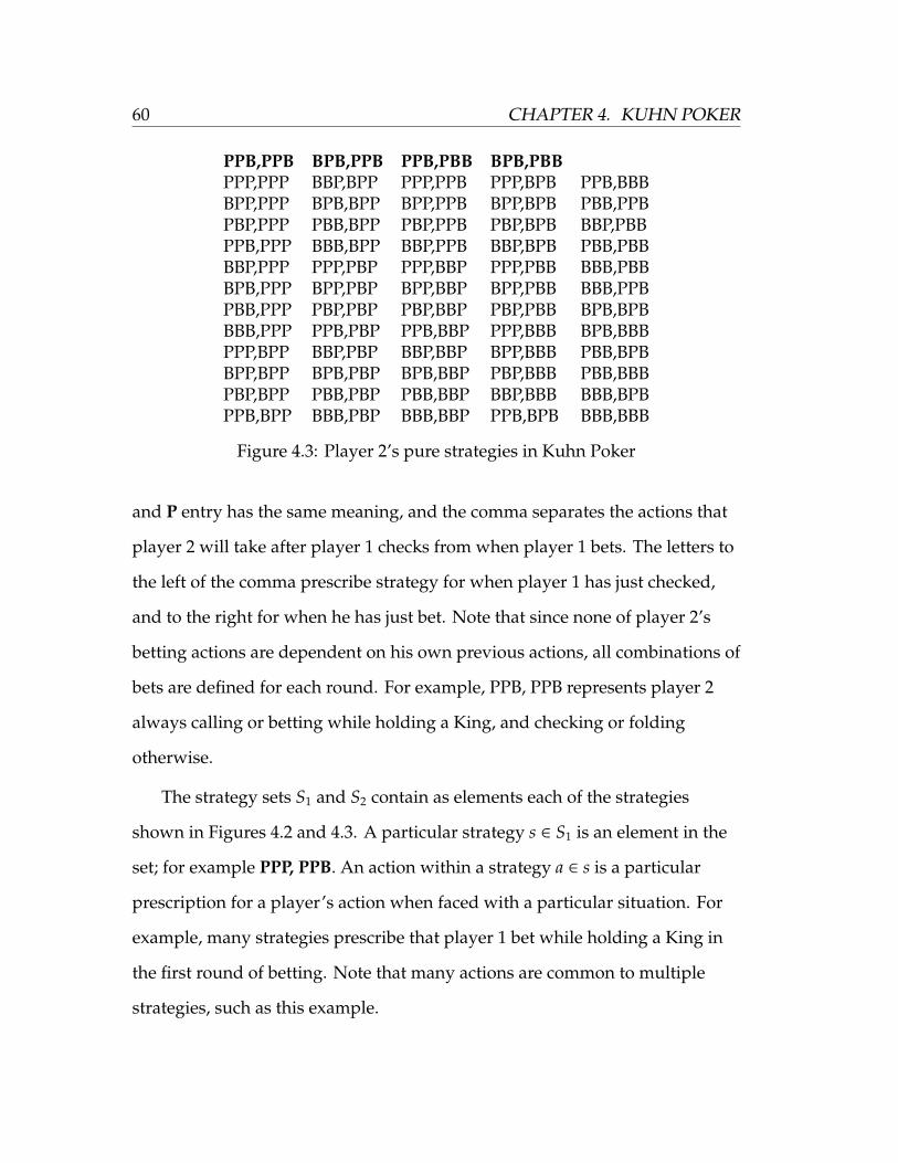
60 CHAPTER 4. KUHN POKER
PPB,PPB BPB,PPB PPB,PBB BPB,PBBPPP,PPP BBP,BPP PPP,PPB PPP,BPB PPB,BBBBPP,PPP BPB,BPP BPP,PPB BPP,BPB PBB,PPBPBP,PPP PBB,BPP PBP,PPB PBP,BPB BBP,PBBPPB,PPP BBB,BPP BBP,PPB BBP,BPB PBB,PBBBBP,PPP PPP,PBP PPP,BBP PPP,PBB BBB,PBBBPB,PPP BPP,PBP BPP,BBP BPP,PBB BBB,PPBPBB,PPP PBP,PBP PBP,BBP PBP,PBB BPB,BPBBBB,PPP PPB,PBP PPB,BBP PPP,BBB BPB,BBBPPP,BPP BBP,PBP BBP,BBP BPP,BBB PBB,BPBBPP,BPP BPB,PBP BPB,BBP PBP,BBB PBB,BBBPBP,BPP PBB,PBP PBB,BBP BBP,BBB BBB,BPBPPB,BPP BBB,PBP BBB,BBP PPB,BPB BBB,BBB
Figure 4.3: Player 2’s pure strategies in Kuhn Poker
and P entry has the same meaning, and the comma separates the actions that
player 2 will take after player 1 checks from when player 1 bets. The letters to
the left of the comma prescribe strategy for when player 1 has just checked,
and to the right for when he has just bet. Note that since none of player 2’s
betting actions are dependent on his own previous actions, all combinations of
bets are defined for each round. For example, PPB, PPB represents player 2
always calling or betting while holding a King, and checking or folding
otherwise.
The strategy sets S1 and S2 contain as elements each of the strategies
shown in Figures 4.2 and 4.3. A particular strategy s ∈ S1 is an element in the
set; for example PPP, PPB. An action within a strategy a ∈ s is a particular
prescription for a player’s action when faced with a particular situation. For
example, many strategies prescribe that player 1 bet while holding a King in
the first round of betting. Note that many actions are common to multiple
strategies, such as this example.
CHAPTER 4. KUHN POKER 61
Each player in Kuhn Poker has many weakly dominated strategies, which
typically stem from a particular action a that is never advantageous to do.
Since the purpose of our analysis is to determine the optimal strategy for each
player, we can ignore these weakly dominated strategies. These can be
identified intuitively. For example, we can eliminate all of player 1’s strategies
involving folding a King after player 2 has bet. Player 1 will always win at
showdown with that hand, and gives up their ante by folding. Thus, those
strategies are weakly dominated by all others. We also eliminate any player 1
strategy that calls a bet with a Jack, bets in the first round with a Queen, as
well as any player 2 strategy that prescribes a bet with a Queen after player 1
has passed. In these last two cases, the player has nothing to gain by betting
with a Queen; the opposing player will always pass with a worse hand (a Jack)
and bet with a better hand (a King). In each case, the payoff expectation is at
least as great if the player passes while holding a Queen. The bolded strategies
in Figures 4.2 and 4.3 represent the non-weakly dominated strategies.
4.3.2 Payoffs
In order to find the Nash equilibria of Kuhn poker, we must first calculate
the payoffs for the entire strategy set. This corresponds to the normal form
representation, shown in (4.1). This matrix represents the payoffs to player 1
for each pair of pure strategies employed, with player 1 as the row player and
player 2 as the column player. The value in each matrix entry is the overall
payoff of the game to player 1; since this is a zero-sum game, the payoffs to
player 2 are simply the corresponding negatives. Each matrix entry is the sum
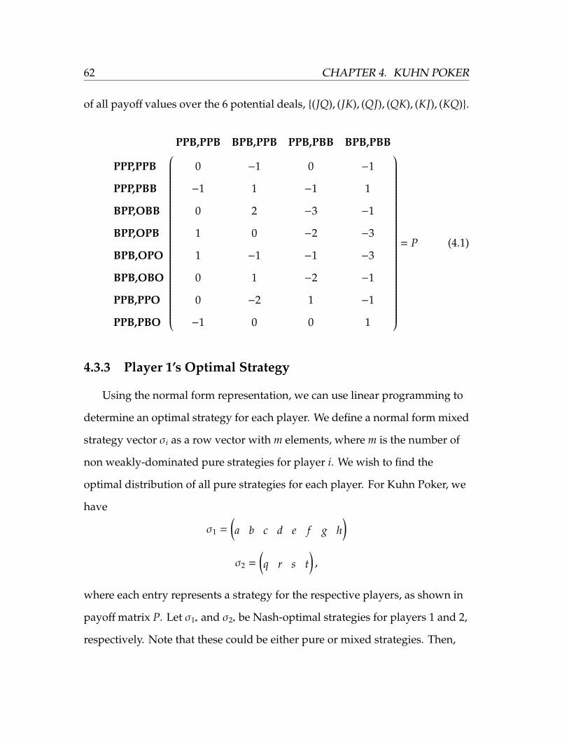
62 CHAPTER 4. KUHN POKER
of all payoff values over the 6 potential deals, {(JQ), (JK), (QJ), (QK), (KJ), (KQ)}.
PPB,PPB BPB,PPB PPB,PBB BPB,PBB
PPP,PPB 0 −1 0 −1
PPP,PBB −1 1 −1 1
BPP,OBB 0 2 −3 −1
BPP,OPB 1 0 −2 −3
BPB,OPO 1 −1 −1 −3
BPB,OBO 0 1 −2 −1
PPB,PPO 0 −2 1 −1
PPB,PBO −1 0 0 1
= P (4.1)
4.3.3 Player 1’s Optimal Strategy
Using the normal form representation, we can use linear programming to
determine an optimal strategy for each player. We define a normal form mixed
strategy vector σi as a row vector with m elements, where m is the number of
non weakly-dominated pure strategies for player i. We wish to find the
optimal distribution of all pure strategies for each player. For Kuhn Poker, we
have
σ1 =(a b c d e f g h
)σ2 =
(q r s t
),
where each entry represents a strategy for the respective players, as shown in
payoff matrix P. Let σ1∗ and σ2∗ be Nash-optimal strategies for players 1 and 2,
respectively. Note that these could be either pure or mixed strategies. Then,
CHAPTER 4. KUHN POKER 63
σk1∗ is the probability that player 1 will play a particular pure strategy k. Note
that the sum of all of the pure strategy probabilities must sum to 1;
∑k
σk1∗ = 1 ,
∑k
σk2∗ = 1. (4.2)
For example, a valid pure strategy for player 1 would be
σ1 =(0 1 0 0 0 0 0 0
),
and a valid mixed strategy for player 2 would be
σ2 =(
12 0 1
2 0).
This particular σ1 denotes always employing PPP,PBB, and σ2 denotes
employing PPB,PPB and PPB,PBB with equal frequency. Note that in both
cases the entries of σ sum to 1, as per (4.2).
Let M as the normal form payoff matrix P with a constant of 4 added to
each entry to make each positive. Define z∗ as the expected value of the game
with payoff matrix P, and z as the expected value of the game with payoff
matrix M. Both z and z∗ are from player 1’s perspective. The reason for this
modification of P will soon become clear; in short, it allows us to define
necessary sign restrictions on our LP. This does not change the optimal
strategy, as it holds the relative payoffs between the two players constant.
However, the optimal objective function value z that we find in the LP will
differ from the true expected value of the game z∗. We later find z∗ through a
different method; the purpose of this analysis is to find the probabilities
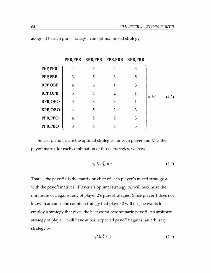
64 CHAPTER 4. KUHN POKER
assigned to each pure strategy in an optimal mixed strategy.
PPB,PPB BPB,PPB PPB,PBB BPB,PBB
PPP,PPB 4 3 4 3
PPP,PBB 3 5 3 5
BPP,OBB 4 6 1 3
BPP,OPB 5 4 2 1
BPB,OPO 5 3 3 1
BPB,OBO 4 5 2 3
PPB,PPO 4 5 2 3
PPB,PBO 3 4 4 5
= M (4.3)
Since σ1∗ and σ2∗ are the optimal strategies for each player and M is the
payoff matrix for each combination of those strategies, we have
σ1∗MσT2∗ = z. (4.4)
That is, the payoff z is the matrix product of each player’s mixed strategy σ
with the payoff matrix P. Player 1’s optimal strategy σ1∗ will maximize the
minimum of z against any of player 2’s pure strategies. Since player 1 does not
know in advance the counter-strategy that player 2 will use, he wants to
employ a strategy that gives the best worst-case scenario payoff. An arbitrary
strategy of player 1 will have at best expected payoff z against an arbitrary
strategy σ2;
σ1MσT2 ≤ z. (4.5)
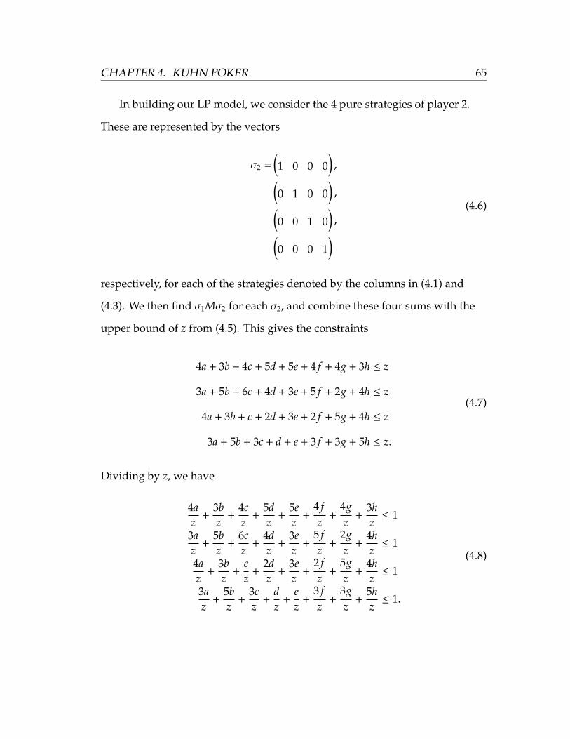
CHAPTER 4. KUHN POKER 65
In building our LP model, we consider the 4 pure strategies of player 2.
These are represented by the vectors
σ2 =(1 0 0 0
),(
0 1 0 0),(
0 0 1 0),(
0 0 0 1)
(4.6)
respectively, for each of the strategies denoted by the columns in (4.1) and
(4.3). We then find σ1Mσ2 for each σ2, and combine these four sums with the
upper bound of z from (4.5). This gives the constraints
4a + 3b + 4c + 5d + 5e + 4 f + 4g + 3h ≤ z
3a + 5b + 6c + 4d + 3e + 5 f + 2g + 4h ≤ z
4a + 3b + c + 2d + 3e + 2 f + 5g + 4h ≤ z
3a + 5b + 3c + d + e + 3 f + 3g + 5h ≤ z.
(4.7)
Dividing by z, we have
4az
+3bz
+4cz
+5dz
+5ez
+4 fz
+4gz
+3hz≤ 1
3az
+5bz
+6cz
+4dz
+3ez
+5 fz
+2gz
+4hz≤ 1
4az
+3bz
+cz
+2dz
+3ez
+2 fz
+5gz
+4hz≤ 1
3az
+5bz
+3cz
+dz
+ez
+3 fz
+3gz
+5hz≤ 1.
(4.8)
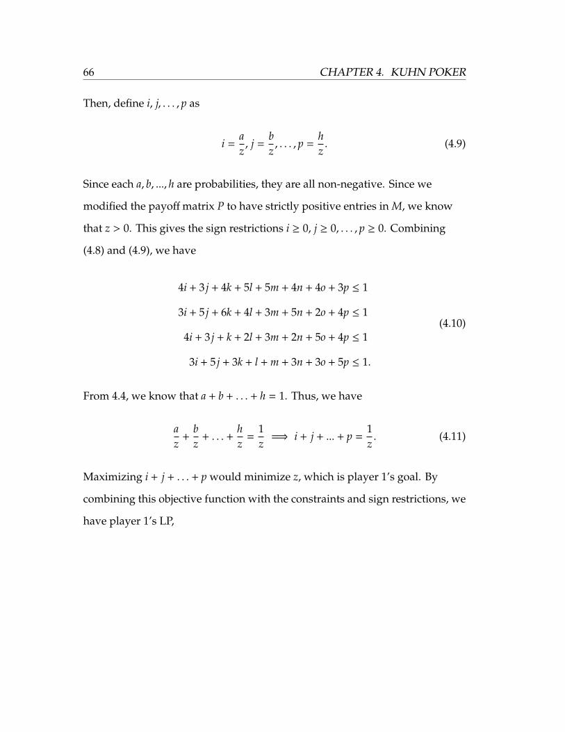
66 CHAPTER 4. KUHN POKER
Then, define i, j, . . . , p as
i =az, j =
bz, . . . , p =
hz. (4.9)
Since each a, b, ..., h are probabilities, they are all non-negative. Since we
modified the payoff matrix P to have strictly positive entries in M, we know
that z > 0. This gives the sign restrictions i ≥ 0, j ≥ 0, . . . , p ≥ 0. Combining
(4.8) and (4.9), we have
4i + 3 j + 4k + 5l + 5m + 4n + 4o + 3p ≤ 1
3i + 5 j + 6k + 4l + 3m + 5n + 2o + 4p ≤ 1
4i + 3 j + k + 2l + 3m + 2n + 5o + 4p ≤ 1
3i + 5 j + 3k + l + m + 3n + 3o + 5p ≤ 1.
(4.10)
From 4.4, we know that a + b + . . . + h = 1. Thus, we have
az
+bz
+ . . . +hz
=1z
=⇒ i + j + ... + p =1z. (4.11)
Maximizing i + j + . . . + p would minimize z, which is player 1’s goal. By
combining this objective function with the constraints and sign restrictions, we
have player 1’s LP,
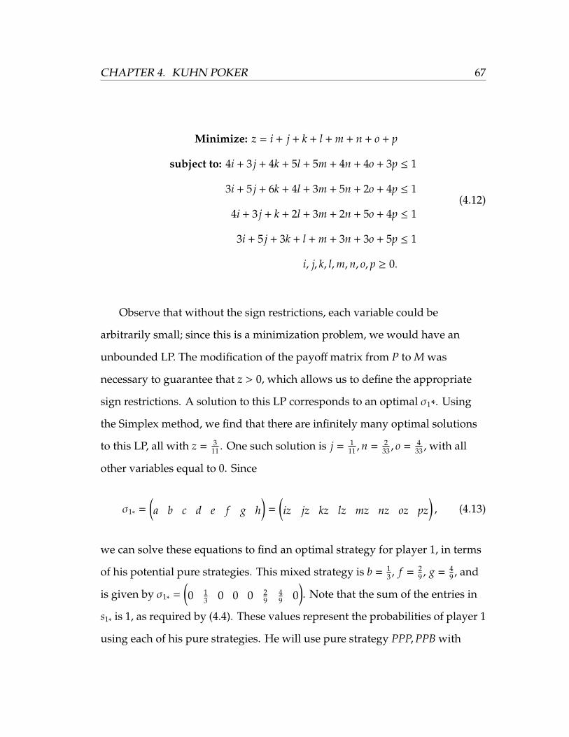
CHAPTER 4. KUHN POKER 67
Minimize: z = i + j + k + l + m + n + o + p
subject to: 4i + 3 j + 4k + 5l + 5m + 4n + 4o + 3p ≤ 1
3i + 5 j + 6k + 4l + 3m + 5n + 2o + 4p ≤ 1
4i + 3 j + k + 2l + 3m + 2n + 5o + 4p ≤ 1
3i + 5 j + 3k + l + m + 3n + 3o + 5p ≤ 1
i, j, k, l,m,n, o, p ≥ 0.
(4.12)
Observe that without the sign restrictions, each variable could be
arbitrarily small; since this is a minimization problem, we would have an
unbounded LP. The modification of the payoff matrix from P to M was
necessary to guarantee that z > 0, which allows us to define the appropriate
sign restrictions. A solution to this LP corresponds to an optimal σ1∗. Using
the Simplex method, we find that there are infinitely many optimal solutions
to this LP, all with z = 311 . One such solution is j = 1
11 ,n = 233 , o = 4
33 , with all
other variables equal to 0. Since
σ1∗ =(a b c d e f g h
)=
(iz jz kz lz mz nz oz pz
), (4.13)
we can solve these equations to find an optimal strategy for player 1, in terms
of his potential pure strategies. This mixed strategy is b = 13 , f = 2
9 , g = 49 , and
is given by σ1∗ =(0 1
3 0 0 0 29
49 0
). Note that the sum of the entries in
s1∗ is 1, as required by (4.4). These values represent the probabilities of player 1
using each of his pure strategies. He will use pure strategy PPP,PPB with
68 CHAPTER 4. KUHN POKER
probability 13 , BPB,OBO with probability 2
9 , and PPB,PPO with probability 49 .
This corresponds to the following mixed strategy. In the first betting round,
Player 1 will bet with probability 29 with a Jack, always pass with a Queen, and
bet with probability 23 with a King. On the second betting round for player 1,
he should always fold a Jack facing a bet, call with a Queen with probability 59 ,
and always call with a King. The other optimal solutions prescribe a similar
strategy; player 1 should vary bluffing with a Jack and slowplaying with a
King. In poker, slowplaying involves checking with a good hand to induce the
other player to bluff with a poor hand.
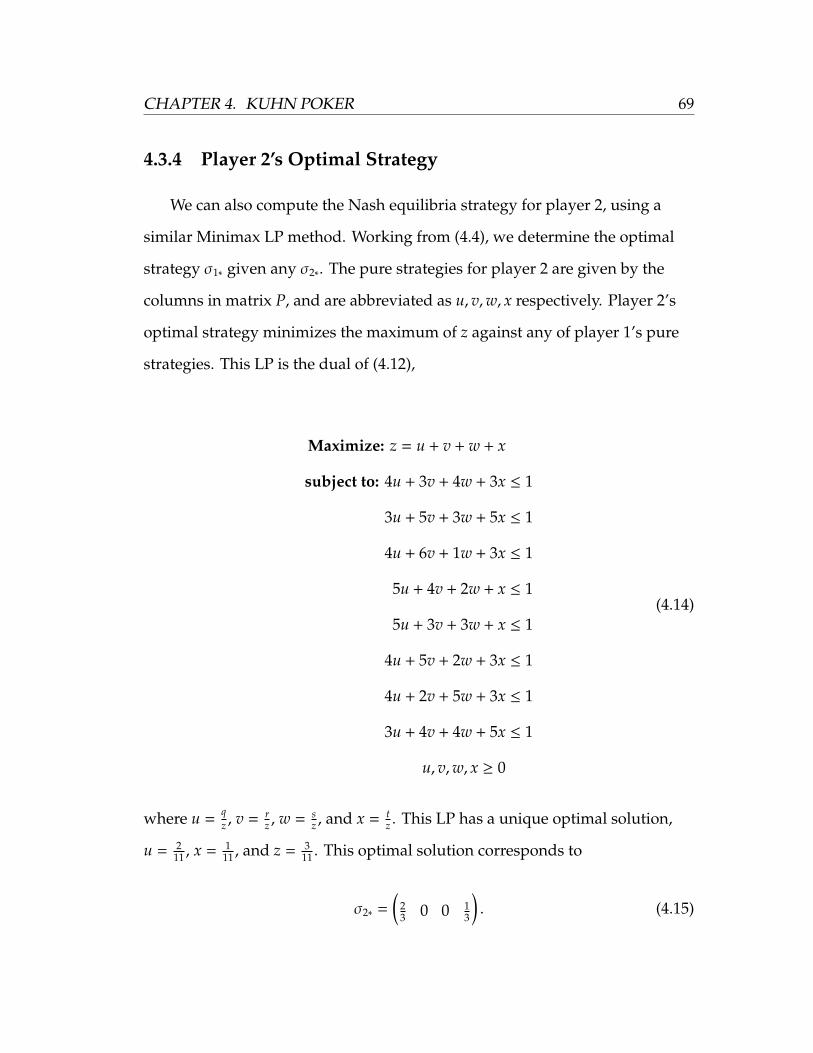
CHAPTER 4. KUHN POKER 69
4.3.4 Player 2’s Optimal Strategy
We can also compute the Nash equilibria strategy for player 2, using a
similar Minimax LP method. Working from (4.4), we determine the optimal
strategy σ1∗ given any σ2∗. The pure strategies for player 2 are given by the
columns in matrix P, and are abbreviated as u, v,w, x respectively. Player 2’s
optimal strategy minimizes the maximum of z against any of player 1’s pure
strategies. This LP is the dual of (4.12),
Maximize: z = u + v + w + x
subject to: 4u + 3v + 4w + 3x ≤ 1
3u + 5v + 3w + 5x ≤ 1
4u + 6v + 1w + 3x ≤ 1
5u + 4v + 2w + x ≤ 1
5u + 3v + 3w + x ≤ 1
4u + 5v + 2w + 3x ≤ 1
4u + 2v + 5w + 3x ≤ 1
3u + 4v + 4w + 5x ≤ 1
u, v,w, x ≥ 0
(4.14)
where u =qz , v = r
z , w = sz , and x = t
z . This LP has a unique optimal solution,
u = 211 , x = 1
11 , and z = 311 . This optimal solution corresponds to
σ2∗ =(
23 0 0 1
3
). (4.15)
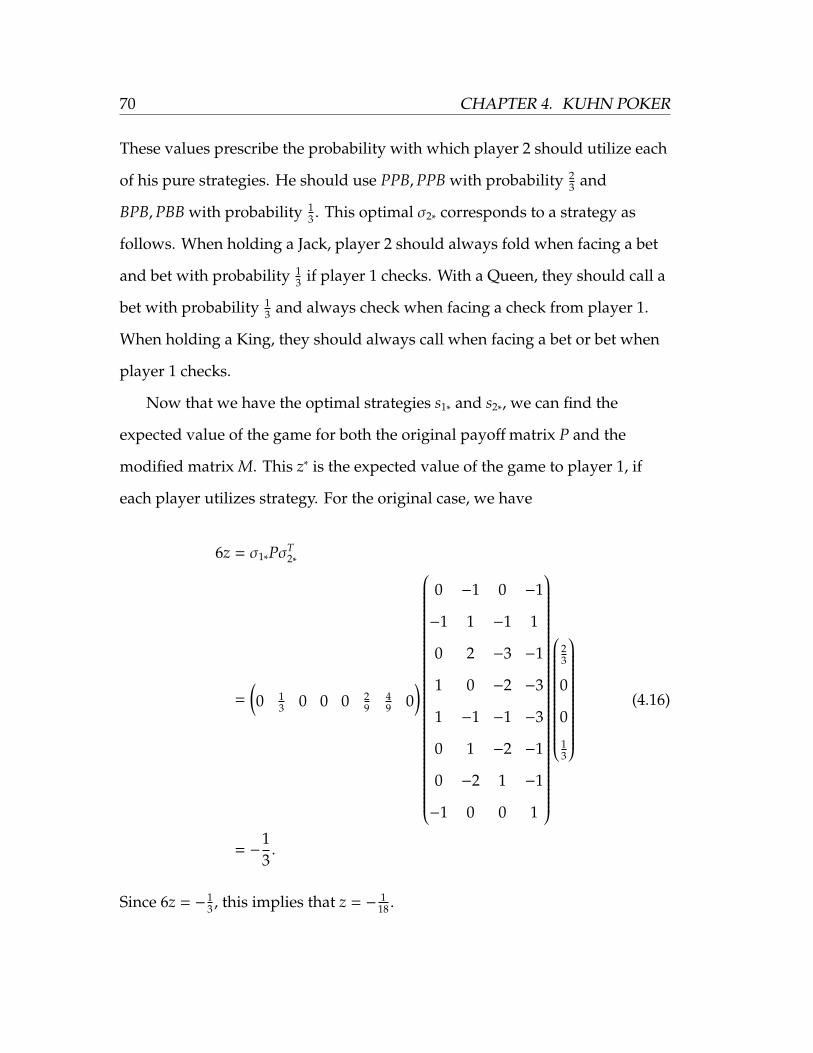
70 CHAPTER 4. KUHN POKER
These values prescribe the probability with which player 2 should utilize each
of his pure strategies. He should use PPB,PPB with probability 23 and
BPB,PBB with probability 13 . This optimal σ2∗ corresponds to a strategy as
follows. When holding a Jack, player 2 should always fold when facing a bet
and bet with probability 13 if player 1 checks. With a Queen, they should call a
bet with probability 13 and always check when facing a check from player 1.
When holding a King, they should always call when facing a bet or bet when
player 1 checks.
Now that we have the optimal strategies s1∗ and s2∗, we can find the
expected value of the game for both the original payoff matrix P and the
modified matrix M. This z∗ is the expected value of the game to player 1, if
each player utilizes strategy. For the original case, we have
6z = σ1∗PσT2∗
=(0 1
3 0 0 0 29
49 0
)
0 −1 0 −1
−1 1 −1 1
0 2 −3 −1
1 0 −2 −3
1 −1 −1 −3
0 1 −2 −1
0 −2 1 −1
−1 0 0 1
23
0
0
13
= −13.
(4.16)
Since 6z = −13 , this implies that z = − 1
18 .
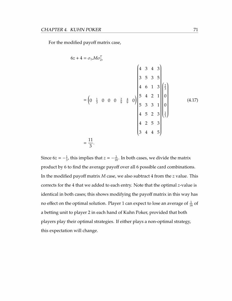
CHAPTER 4. KUHN POKER 71
For the modified payoff matrix case,
6z + 4 = σ1∗MσT2∗
=(0 1
3 0 0 0 29
49 0
)
4 3 4 3
3 5 3 5
4 6 1 3
5 4 2 1
5 3 3 1
4 5 2 3
4 2 5 3
3 4 4 5
23
0
0
13
=113.
(4.17)
Since 6z = −13 , this implies that z = − 1
18 . In both cases, we divide the matrix
product by 6 to find the average payoff over all 6 possible card combinations.
In the modified payoff matrix M case, we also subtract 4 from the z value. This
corrects for the 4 that we added to each entry. Note that the optimal z-value is
identical in both cases; this shows modifying the payoff matrix in this way has
no effect on the optimal solution. Player 1 can expect to lose an average of 118 of
a betting unit to player 2 in each hand of Kuhn Poker, provided that both
players play their optimal strategies. If either plays a non-optimal strategy,
this expectation will change.
72 CHAPTER 4. KUHN POKER
4.4 Sequence Form
The normal form representation provides a succinct correspondence with
an LP, particularly for small games. However, this model quickly becomes
intractable for large games. While the normal form payoff matrix is generally
exponential with the size of the game tree, growth in the sequence form is at
most linear [13]. As such, the sequence form representation is more
appropriate for larger games. This difference is not as apparent in the
sequence form representation of Kuhn Poker, as it is a relatively small game.
This will become more apparent in Chapter 5, when we consider a much
larger game. This section applies the theory of Section 3.4 to Kuhn Poker. We
define and solve linear programs to find the optimal strategies (as realization
plans) for each player.
4.4.1 Sequences and Information Sets
Recall that a fundamental concept in the sequence form representation is
the information set. An information set in an imperfect information game is a
set of possible game states that are identical from the point of view of a
particular player. In Kuhn Poker, an information set for a player consists in
knowing what card they hold as well as the betting sequence thus far in the
hand. They do not know what card their opponent holds. Since there is
hidden information throughout the game, there are multiple elements in each
information set. Note that distinct elements in an information set can
represent very different positions on the game tree. Different nodes represent
distinct positions on the game tree, but nodes in the same information set are
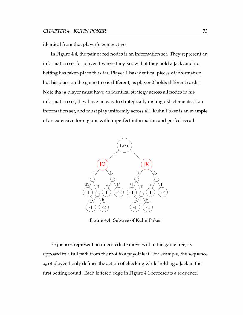
CHAPTER 4. KUHN POKER 73
identical from that player’s perspective.
In Figure 4.4, the pair of red nodes is an information set. They represent an
information set for player 1 where they know that they hold a Jack, and no
betting has taken place thus far. Player 1 has identical pieces of information
but his place on the game tree is different, as player 2 holds different cards.
Note that a player must have an identical strategy across all nodes in his
information set; they have no way to strategically distinguish elements of an
information set, and must play uniformly across all. Kuhn Poker is an example
of an extensive form game with imperfect information and perfect recall.
Deal
JQ
-1
-1 -2
1 -2
JK
-1
-1 -2
1 -2
a
m n
g h
b
o p
a
q r
g h
b
s t
Figure 4.4: Subtree of Kuhn Poker
Sequences represent an intermediate move within the game tree, as
opposed to a full path from the root to a payoff leaf. For example, the sequence
xa of player 1 only defines the action of checking while holding a Jack in the
first betting round. Each lettered edge in Figure 4.1 represents a sequence.
74 CHAPTER 4. KUHN POKER
Note that each player in Kuhn Poker has a unique set of sequences, given by
S0 = {s∅},
S1 =
l⋃i=a
si,
S2 =
x⋃i=m
si,
The S0 set represents the chance player, who initializes the game at the root by
generating a random deal of the cards for each player.
4.4.2 Payoffs
We now turn our attention to defining the payoff matrix P in the sequence
form representation of Kuhn Poker. Since the payoffs at each leaf are unique to
their preceding sequences, the payoff function g is well defined. There are at
most as many sequences as nodes for a particular player, so the number of
sequences is linear in the size of the game tree. Since the number of nonzero
entries of this matrix is at most the number of sequences of player i, this matrix
is sparse. Most entries will be 0, as they represent combinations of sequences
that are not possible and have no associated payoff [13]. Consider
g(s∅, sa, so) = 0; this defines the payoff to player 1 checking while holding a Jack
and player 2 betting while holding a Queen after player 1 has bet. Since this
combination is not possible, the payoff is 0. Examining Figure 4.1, we can see
that most combinations of sequences s are impossible and are assigned a
payoff of 0 by default.
In Kuhn Poker, we consider g(s∅, s1, s2) to be the payoff to player 1 from
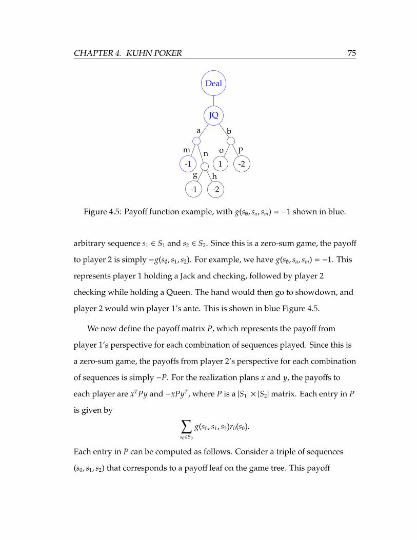
CHAPTER 4. KUHN POKER 75
Deal
JQ
-1
-1 -2
1 -2
a
m n
g h
b
o p
Figure 4.5: Payoff function example, with g(s∅, sa, sm) = −1 shown in blue.
arbitrary sequence s1 ∈ S1 and s2 ∈ S2. Since this is a zero-sum game, the payoff
to player 2 is simply −g(s∅, s1, s2). For example, we have g(s∅, sa, sm) = −1. This
represents player 1 holding a Jack and checking, followed by player 2
checking while holding a Queen. The hand would then go to showdown, and
player 2 would win player 1’s ante. This is shown in blue Figure 4.5.
We now define the payoff matrix P, which represents the payoff from
player 1’s perspective for each combination of sequences played. Since this is
a zero-sum game, the payoffs from player 2’s perspective for each combination
of sequences is simply −P. For the realization plans x and y, the payoffs to
each player are xTPy and −xPyT, where P is a |S1| × |S2|matrix. Each entry in P
is given by ∑s0∈S0
g(s0, s1, s2)r0(s0).
Each entry in P can be computed as follows. Consider a triple of sequences
(s0, s1, s2) that corresponds to a payoff leaf on the game tree. This payoff
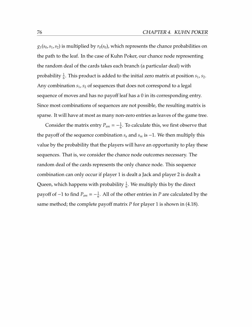
76 CHAPTER 4. KUHN POKER
g1(s0, s1, s2) is multiplied by r0(s0), which represents the chance probabilities on
the path to the leaf. In the case of Kuhn Poker, our chance node representing
the random deal of the cards takes each branch (a particular deal) with
probability 16 . This product is added to the initial zero matrix at position s1, s2.
Any combination s1, s2 of sequences that does not correspond to a legal
sequence of moves and has no payoff leaf has a 0 in its corresponding entry.
Since most combinations of sequences are not possible, the resulting matrix is
sparse. It will have at most as many non-zero entries as leaves of the game tree.
Consider the matrix entry Pam = −16 . To calculate this, we first observe that
the payoff of the sequence combination sa and sm is −1. We then multiply this
value by the probability that the players will have an opportunity to play these
sequences. That is, we consider the chance node outcomes necessary. The
random deal of the cards represents the only chance node. This sequence
combination can only occur if player 1 is dealt a Jack and player 2 is dealt a
Queen, which happens with probability 16 . We multiply this by the direct
payoff of −1 to find Pam = − 16 . All of the other entries in P are calculated by the
same method; the complete payoff matrix P for player 1 is shown in (4.18).
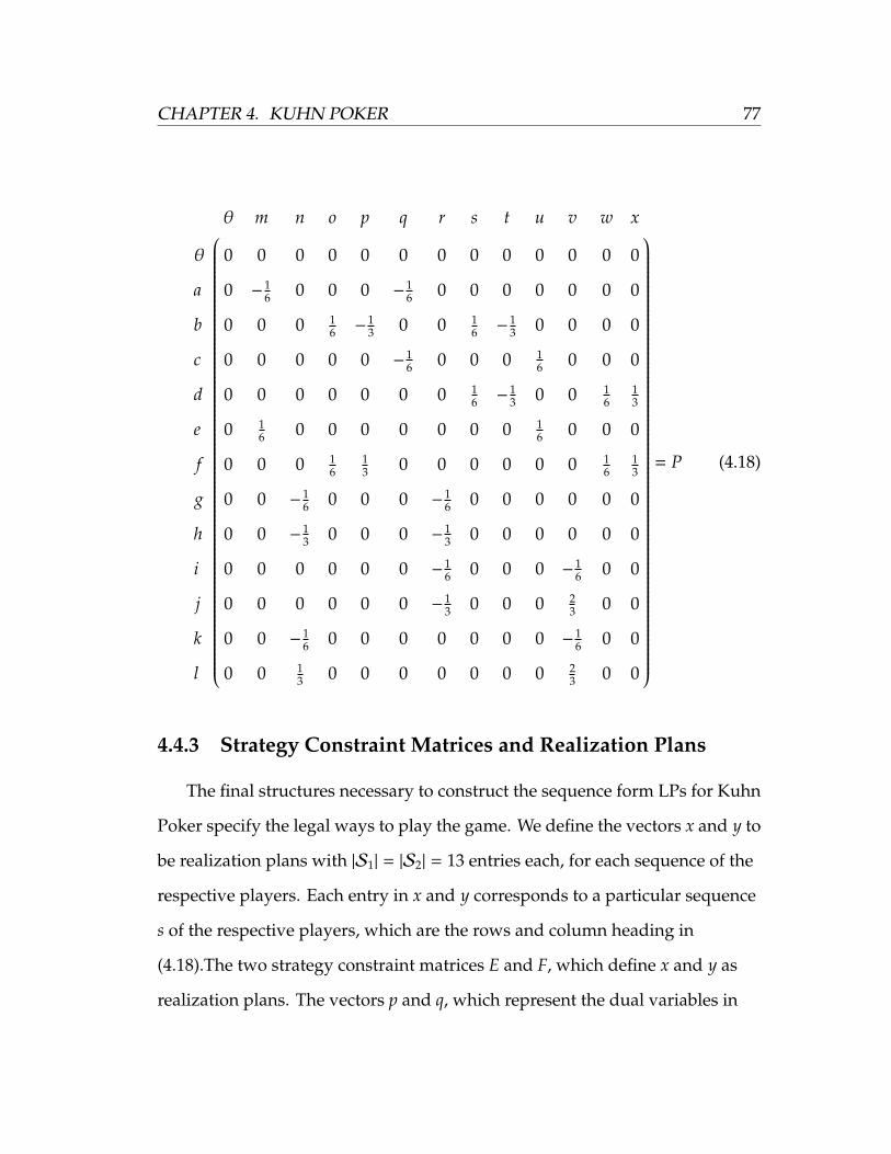
CHAPTER 4. KUHN POKER 77
θ m n o p q r s t u v w x
θ 0 0 0 0 0 0 0 0 0 0 0 0 0
a 0 −16 0 0 0 −
16 0 0 0 0 0 0 0
b 0 0 0 16 −
13 0 0 1
6 −13 0 0 0 0
c 0 0 0 0 0 −16 0 0 0 1
6 0 0 0
d 0 0 0 0 0 0 0 16 −
13 0 0 1
613
e 0 16 0 0 0 0 0 0 0 1
6 0 0 0
f 0 0 0 16
13 0 0 0 0 0 0 1
613
g 0 0 −16 0 0 0 −
16 0 0 0 0 0 0
h 0 0 −13 0 0 0 −
13 0 0 0 0 0 0
i 0 0 0 0 0 0 −16 0 0 0 −
16 0 0
j 0 0 0 0 0 0 −13 0 0 0 2
3 0 0
k 0 0 −16 0 0 0 0 0 0 0 −
16 0 0
l 0 0 13 0 0 0 0 0 0 0 2
3 0 0
= P (4.18)
4.4.3 Strategy Constraint Matrices and Realization Plans
The final structures necessary to construct the sequence form LPs for Kuhn
Poker specify the legal ways to play the game. We define the vectors x and y to
be realization plans with |S1| = |S2| = 13 entries each, for each sequence of the
respective players. Each entry in x and y corresponds to a particular sequence
s of the respective players, which are the rows and column heading in
(4.18).The two strategy constraint matrices E and F, which define x and y as
realization plans. The vectors p and q, which represent the dual variables in
78 CHAPTER 4. KUHN POKER
each LP; they have 1 + |I1| and 1 + |I2| entries respectively. Finally, we have
vectors e and f , which are unit vectors of an appropriate dimension that satisfy
Ex = e and Fy = y. These elements are based on the properties of realization
plans in (3.4), (3.5), and (3.6).
The strategy constraint matrices E and F define the legal combinations of
sequences that each player can choose. The dimensions of E and F are
(1 + |I1|) × |S1| and (1 + |I2|) × |S2|. Since each player has 6 information sets
and 13 sequences, both matrices are 7 × 13. Each row in these matrices
represent a particular information set, and each column represents a particular
sequence. The fact that both matrices are the same size is a coincidence based
on the structure of Kuhn Poker, as both player 1 and player 2 happen to have 6
information sets and 12 sequences. The first row in E and F represents the 0th
information set corresponding to the random deal, and the first column
represents the sequence s∅ of the random deal.
These matrices can be constructed as follows. We place a 1 in this first
entry to initialize the game. For each subsequent information set row, we place
a −1 in the sequence that is required to happen before the player is in the
information set. Then, we place a 1 in each sequence in the information set.
For example, sequence sa must occur before player 1 can be in information set
4 where he can choose to play sequence g or h. Since the previous “move” for
player 2 is the random deal θ, each information set row in F initializes with a
−1 at θ. Using this process, we have E and F as shown in (4.19) and (4.20).
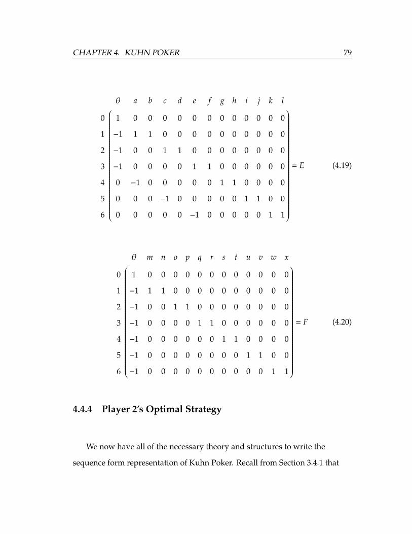
CHAPTER 4. KUHN POKER 79
θ a b c d e f g h i j k l
0 1 0 0 0 0 0 0 0 0 0 0 0 0
1 −1 1 1 0 0 0 0 0 0 0 0 0 0
2 −1 0 0 1 1 0 0 0 0 0 0 0 0
3 −1 0 0 0 0 1 1 0 0 0 0 0 0
4 0 −1 0 0 0 0 0 1 1 0 0 0 0
5 0 0 0 −1 0 0 0 0 0 1 1 0 0
6 0 0 0 0 0 −1 0 0 0 0 0 1 1
= E (4.19)
θ m n o p q r s t u v w x
0 1 0 0 0 0 0 0 0 0 0 0 0 0
1 −1 1 1 0 0 0 0 0 0 0 0 0 0
2 −1 0 0 1 1 0 0 0 0 0 0 0 0
3 −1 0 0 0 0 1 1 0 0 0 0 0 0
4 −1 0 0 0 0 0 0 1 1 0 0 0 0
5 −1 0 0 0 0 0 0 0 0 1 1 0 0
6 −1 0 0 0 0 0 0 0 0 0 0 1 1
= F (4.20)
4.4.4 Player 2’s Optimal Strategy
We now have all of the necessary theory and structures to write the
sequence form representation of Kuhn Poker. Recall from Section 3.4.1 that

80 CHAPTER 4. KUHN POKER
player 2’s optimal realization plan is the solution to
Minimize: f (x, q) = −qT f
subject to: xT(−P) − qTF ≤ 0
xTET = eT
x ≥ 0.
(4.21)
With the structures defined in the previous sections, our LP is
Minimize: q0
subject to: q0 − q1 − q2 − q3 ≥ 0
16
xm +16
xr + q2 − q4 ≥ 0
−16
x∅ +13
xp −16
xs +13
xt + q1 ≥ 0
16
xq −16
xu + q2 − q5 ≥ 0
−16
xs +13
xt −16
xw −13
xx + q2 ≥ 0
−16
xm −16
xu + q3 − q6 ≥ 0
−16
xo −13
xp −16
xw −13
xx + q3 ≥ 0
16
xn +16
xr + q4 ≥ 0
13
xn +13
xr + q4 ≥ 0
16
xr +16
xv + q5 ≥ 0
13
xr −13
xv + q5 ≥ 0
(4.22)
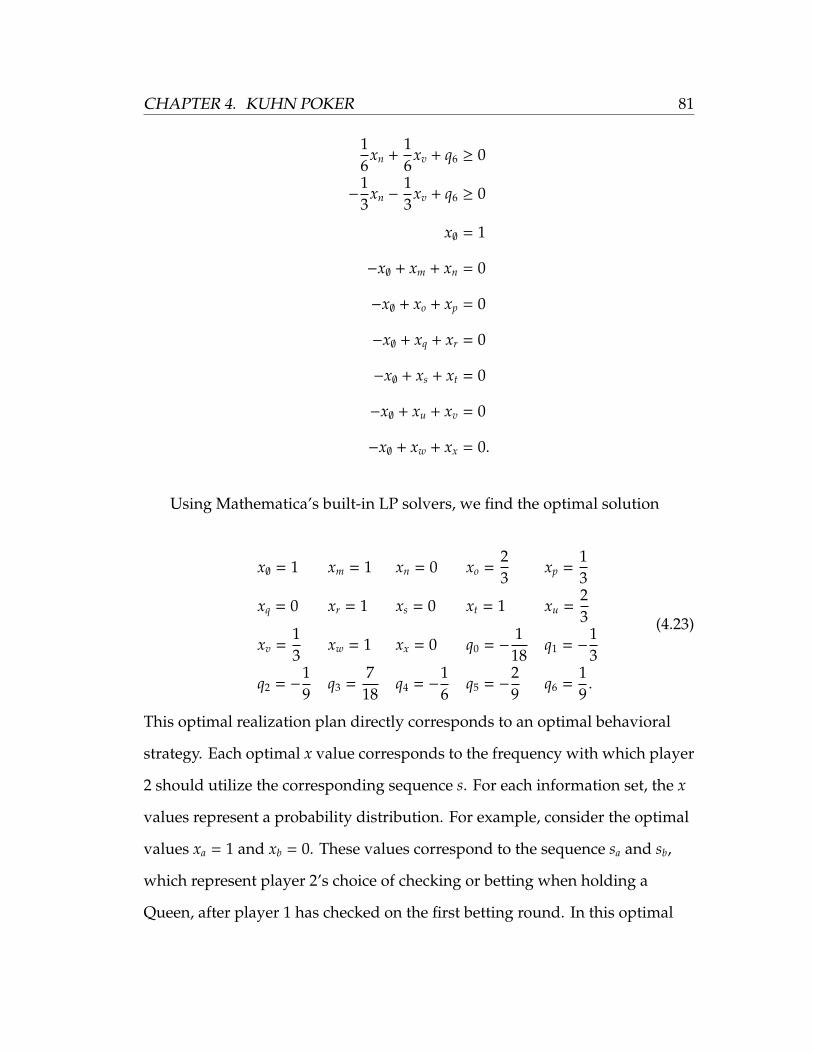
CHAPTER 4. KUHN POKER 81
16
xn +16
xv + q6 ≥ 0
−13
xn −13
xv + q6 ≥ 0
x∅ = 1
−x∅ + xm + xn = 0
−x∅ + xo + xp = 0
−x∅ + xq + xr = 0
−x∅ + xs + xt = 0
−x∅ + xu + xv = 0
−x∅ + xw + xx = 0.
Using Mathematica’s built-in LP solvers, we find the optimal solution
x∅ = 1 xm = 1 xn = 0 xo =23
xp =13
xq = 0 xr = 1 xs = 0 xt = 1 xu =23
xv =13
xw = 1 xx = 0 q0 = −118
q1 = −13
q2 = −19
q3 =718
q4 = −16
q5 = −29
q6 =19.
(4.23)
This optimal realization plan directly corresponds to an optimal behavioral
strategy. Each optimal x value corresponds to the frequency with which player
2 should utilize the corresponding sequence s. For each information set, the x
values represent a probability distribution. For example, consider the optimal
values xa = 1 and xb = 0. These values correspond to the sequence sa and sb,
which represent player 2’s choice of checking or betting when holding a
Queen, after player 1 has checked on the first betting round. In this optimal
82 CHAPTER 4. KUHN POKER
strategy, player 2 should always choose sequence sa. This makes intuitive
sense; if player 2 bets in this situation, player 1 will always call the bet when
holding a King, and fold when holding a Jack. In both cases, player 2 is better
off choosing not to bet. The action of player 2 betting while holding a Queen
after player 1 has checked to him is an example of a weakly-dominated action.
This solution does not prescribe a pure strategy for every information set;
instead, optimal strategy sometimes prescribes a mix of actions. For example,
consider xc = 23 and xd = 1
3 . The corresponding sequences represent player 2’s
betting choice when holding a Queen, and player 1 has just bet. Optimal
strategy dictates that player 2 should pass with probability 23 and bet with
probability 13 . The non-deterministic strategy in that information set means
that the optimal strategy for player 2 is a mixed strategy.
In addition to describing the optimal strategy for player 2, the solution to
this LP also shows the value of Kuhn Poker from player 1’s perspective. The
value of the game is the optimal objective function value, which in this case is
simply q0 = − 118 . Note that this is identical to the optimal z value found using
the normal form LPs. In each hand of Kuhn Poker, player 1 can expect to lose
118 of a betting unit. Note that this is player 1’s expectation only if both players
utilize their Nash optimal strategies; if either deviate, his expectation can
change significantly. It is not surprising that optimally-played Kuhn poker
inherently favors player 2; it is well known that players who act after their
opponent hold an advantage. This is a concept known as “position”, and is
particularly important in poker variants with more rounds of betting.
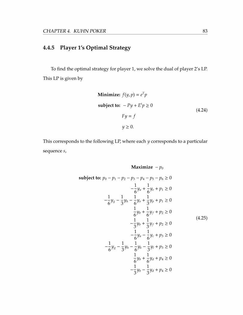
CHAPTER 4. KUHN POKER 83
4.4.5 Player 1’s Optimal Strategy
To find the optimal strategy for player 1, we solve the dual of player 2’s LP.
This LP is given by
Minimize: f (y, p) = eTp
subject to: − Py + Etp ≥ 0
Fy = f
y ≥ 0.
(4.24)
This corresponds to the following LP, where each y corresponds to a particular
sequence s,
Maximize − p0
subject to: p0 − p1 − p2 − p3 − p4 − p5 − p6 ≥ 0
−16
ya +16
ye + p1 ≥ 0
−16
yg −13
yh −16
yo +13
yp + p1 ≥ 0
16
yb +16
y f + p2 ≥ 0
−13
yb +13
y f + p2 ≥ 0
−16
ya −16
yc + p3 ≥ 0
−16
yg −13
yh −16
yk −13
yl + p3 ≥ 0
16
yb +16
yd + p4 ≥ 0
−13
yb −13
yd + p4 ≥ 0
(4.25)
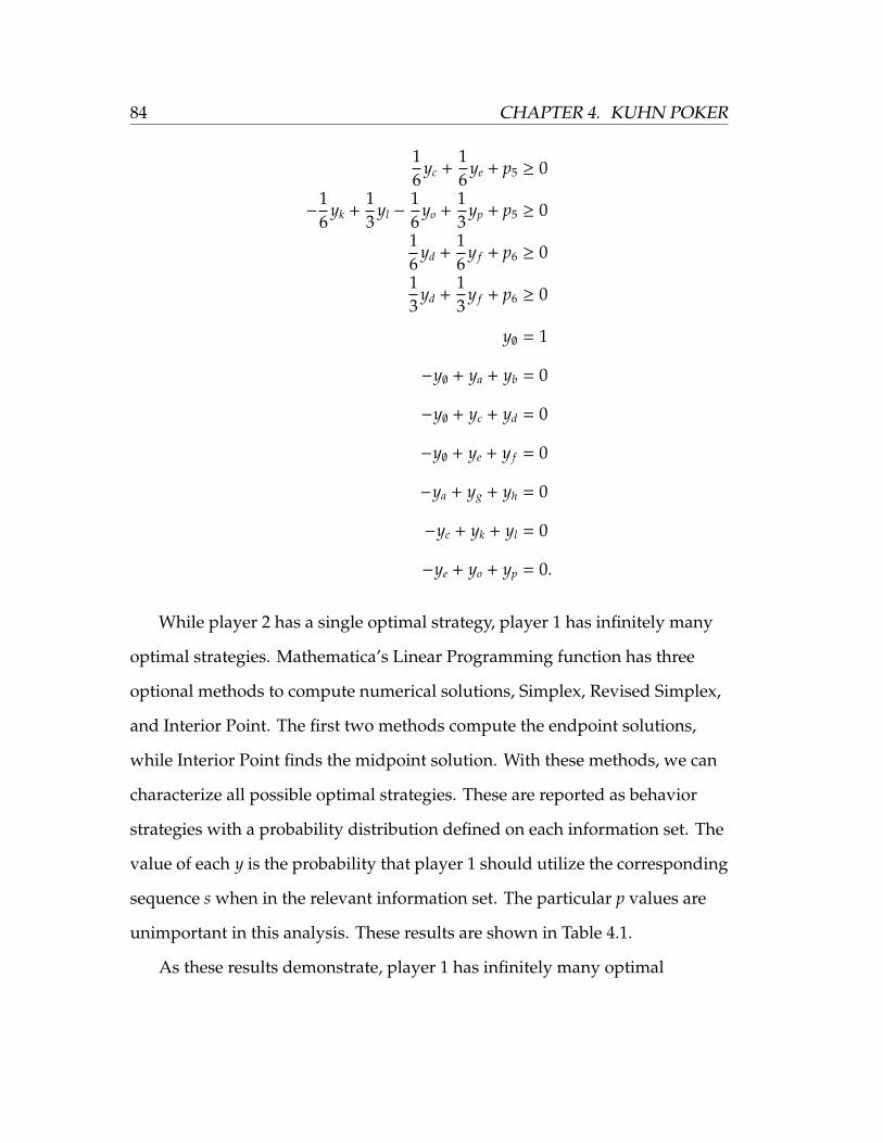
84 CHAPTER 4. KUHN POKER
16
yc +16
ye + p5 ≥ 0
−16
yk +13
yl −16
yo +13
yp + p5 ≥ 0
16
yd +16
y f + p6 ≥ 0
13
yd +13
y f + p6 ≥ 0
y∅ = 1
−y∅ + ya + yb = 0
−y∅ + yc + yd = 0
−y∅ + ye + y f = 0
−ya + yg + yh = 0
−yc + yk + yl = 0
−ye + yo + yp = 0.
While player 2 has a single optimal strategy, player 1 has infinitely many
optimal strategies. Mathematica’s Linear Programming function has three
optional methods to compute numerical solutions, Simplex, Revised Simplex,
and Interior Point. The first two methods compute the endpoint solutions,
while Interior Point finds the midpoint solution. With these methods, we can
characterize all possible optimal strategies. These are reported as behavior
strategies with a probability distribution defined on each information set. The
value of each y is the probability that player 1 should utilize the corresponding
sequence s when in the relevant information set. The particular p values are
unimportant in this analysis. These results are shown in Table 4.1.
As these results demonstrate, player 1 has infinitely many optimal

CHAPTER 4. KUHN POKER 85
Simplex Interior Point Revised Simplex
y∅ 1 1 1
ya 1 56
23
yb 0 16
13
yc 1 1 1
yd 0 0 0
ye 1 12 0
yf 0 12 1
yg 1 56
23
yh 0 0 0
yi23
12
13
yj13
12
23
yk 0 0 0
yl 1 12 0
p0 −1
18 −118 −
118
p1 0 −118 −
19
p2 0 19
29
p3 −7
18 −718 −
718
p4 0 −118 −
19
p513
14
16
p6 0 4215000
16
Table 4.1: Solutions to Player 1’s LP
86 CHAPTER 4. KUHN POKER
strategies. Since the Simplex and Revised Simplex solutions represent the
endpoint solutions, all intermediate solutions are also optimal. We can
characterize player 1’s optimal strategies as dependent on a parameter
α ∈ [0, 13 ], which is the probability that they will bet on their first turn while
holding a Jack. When holding a King, player 1 should bet with probability 3α
on their first turn. When holding a Queen, player 1 should always check on
their first betting round. If player 2 bets after this check, player 1 should call
the bet with probability α + 13 . Finally, player 1 should always fold a Jack and
call with a King when facing a bet from player 2.
Unlike player 1’s LP solution (4.1), player 2’s LP solution does not
correspond neatly to a behavioral strategy. Recall that the optimal values
calculated by the sequence form LP describe a realization plan, which are
relative to the realization probability of an information set. Consider that
player 1 will not always have a second choice to bet; this only occurs when he
checks and player 2 bets. There are many other paths down the game tree that
do not involve these moves, such as both players checking or player 2 folding
to player 1’s bet. Since player 2 always faces a decision to check, bet, or fold
regardless of player 1’s action, the sum of each pair of sequences s for each
information set is 1. The same is not true for player 1, who will not always get
to play sequences sg through sl. Consider the optimal ya = 56 in the Interior
Point solution (α = 16 ). Since player 1’s potential later choice between sg and sl
is dependent on him also playing sa, yg + yl = 56 in the solution to the LP. We use
a similar process to convert each of the values in the realization plan to a full
behavioral strategy. In a sense, the probability of the base sequence (ya = 56 )
becomes the new “1” for its subsequent sequences further down the game tree.
CHAPTER 4. KUHN POKER 87
In player 1’s optimal realization plan, some sequences will never be used.
Consider the sequences sk and sl, both with realization probability 0 in the
Revised Simplex solution. Both are members of the same information set, in
which player 1 was dealt a King, checked initially, and now faces a bet from
player 2. However, he will never reach this information set if he plays
according to other elements of his optimal realization plan. In the Revised
Simplex solution, ye = 0; that is, he never checks initially while holding a King.
Since se is necessary for both sk and sl, he will never face the choice. Therefore,
an optimal realization plan does not have to specify frequencies for these
actions. Table 4.2 shows the optimal realization plan converted to an optimal
behavior strategy as above, with *** denoting sequences that are never reached.
The Simplex solution represents the case α = 0. In this case, player 1
always checks in the first round; that is, ya = yc = ye = 1 and yb = yd = y f = 0.
Since he chooses to never bluff (by betting when holding a Jack), he must
balance his strategy by also never betting a King for value. He must call a bet
from player 2 while holding a Queen with probability 13 . The Revised Simplex
method gives the other endpoint solution, with α = 13 . In this strategy, player 1
bluffs with a Jack with probability 13 (yb = 1
3 ), and always value bets with a
King (y f = 1). He always checks with a Queen in the first round (yc = 1), and
calls a bet from player 2 with probability 23 (y j = 2
3 ). In all optimal strategies,
player 1 folds with a Jack and calls with a King when facing a bet. He cannot
win a showdown with a Jack, and cannot lose a showdown with a King; thus,
any strategy that did not prescribe these sequences is weakly dominated by
those that do. The Simplex solution (α = 0) represents player 1’s most
conservative strategy, as he never bluffs with a Jack and never value bets with
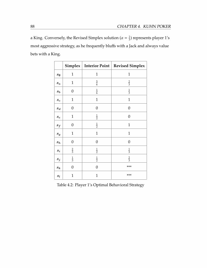
88 CHAPTER 4. KUHN POKER
a King. Conversely, the Revised Simplex solution (α = 13 ) represents player 1’s
most aggressive strategy, as he frequently bluffs with a Jack and always value
bets with a King.
Simplex Interior Point Revised Simplex
s∅ 1 1 1
sa 1 56
23
sb 0 16
13
sc 1 1 1
sd 0 0 0
se 1 12 0
sf 0 12 1
sg 1 1 1
sh 0 0 0
si23
12
13
sj13
12
23
sk 0 0 ***
sl 1 1 ***
Table 4.2: Player 1’s Optimal Behavioral Strategy
Chapter 5
2-7 Draw Poker
Although Kuhn Poker serves as a useful example in understanding
concepts in game theory and the method of the sequence form, it bears little
resemblance to actual variants of poker. Other variants play with more cards,
more betting rounds, and more players. In turn, these games are much more
complex to analyze; for comparison, 2-player no-limit Texas Hold’em has
approximately 10160 information sets [10]. That is many more atoms than exist
in the known universe. While games of this size are significantly beyond the
capabilities of this approach, we are able to analyze abstracted versions of
more complex games. In this chapter, we develop an abstracted version of 2-7
Draw poker and use the sequence form LP methodology to determine an
optimal strategy.
5.1 Rules
While poker variants such as Texas Hold’em and Omaha have become
very popular in recent years, variants such as 2-7 Draw still have a loyal
89

90 CHAPTER 5. 2-7 DRAW POKER
following. Its structure and game play are very different, and little previous
work has been published on game-theoretic optimal play. As such, it is a
fruitful area of research. This section details the rules of full-scale, two player
2-7 Draw based on [8]. 2-7 Draw is a lowball variant, meaning that traditional
hand rankings are reversed; the worst traditional hand wins the pot, if the
hand goes to showdown. Additionally, as the name suggests, it is a draw
variant. Each player is dealt a private hand, and has the opportunity to
discard and redraw any number of their own cards after each betting round.
These features contrast with games such as Texas Hold’em and Omaha, where
players share a common set of community cards and the highest hand wins.
At the start of each hand, each player is dealt 5 cards. There is a round of
betting, where each player has the option to check, bet, raise, or fold,
depending on the actions of previous players. Betting in 2-7 Draw games can
have a limit structure, with fixed bet sizes, or a no-limit betting structure,
where players can bet any amount. Then, each player discards any or all of
their hand, and replaces them with cards from the deck. 2-7 Draw is most
commonly played with one or three discard rounds; our version uses one
discard round. If there is more than one person who has not previously
folded, the hand goes to showdown, and the player with the worst hand wins
the pot. Thus, a hand of 2-7 (Single) Draw has the following structure:
1. Five cards are dealt to each player
2. Betting round #1
3. Discard and redraw (up to 5 cards)
4. Betting round #2
CHAPTER 5. 2-7 DRAW POKER 91
5. Showdown (if necessary)
Hand rankings in 2-7 Draw are reversed in comparison to poker variants
such as Texas Hold’em and Omaha. From best to worst, they are as follows:
1. No Pair
2. One Pair
3. Two Pair
4. Three of a Kind
5. Straight
6. Flush
7. Full House
8. Four of a Kind
9. Straight Flush
10. Royal Flush
Within each of these categories, there is a further ordering. The best possible
No Pair hand is 7, 5, 4, 3, 2, not of the same suit. The best possible One Pair
hand is 2, 2, 5, 4, 3, which is worse than all No Pair hands. Ordering in each
category is determined first by the highest card (or pair), and subsequently by
the next highest card. For example, 4, 4, 4, 2, 2 beats 4, 4, 4, 3, 3. Each category
admits a similar ordering structure.

92 CHAPTER 5. 2-7 DRAW POKER
5.2 Abstractions
In order to analyze a poker variant using the sequence form LP method, it
is necessary to reduce the size of the game. There are several types of these
abstractions, all of which aim to simplify the game without losing the
underlying strategy. The abstractions that we use to simplify 2-7 Draw are
outlined in this section, and are based on ideas from [2].
5.2.1 Deck Reduction
One abstraction technique to reduce the size of the game is to reduce the
number of cards in the deck. This simplifies the game by drastically reducing
the number of potential hands and, by extension, the size of the game tree. For
example, a 52 card deck has
(525
)= 2, 598, 960
unique 5 card hands. In using this type of abstraction, it is important to choose
a deck size that maintains an equivalent ordering of hand strengths. In other
words, the frequencies of each hand category must remain generally
consistent between the original game and the abstraction. For example, One
Pair must be more common than a Straight, which in turn must be more
common than a Flush. To accomplish this, we experimented with several
combinations of deck size and hand size. We settle on a 21 card deck with 3
card hands for each player. This deck contains the cards 2 through 8 of each of
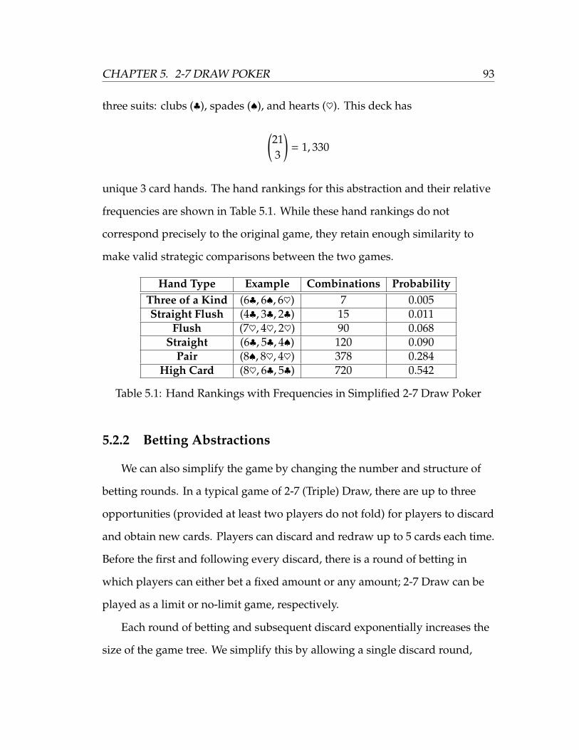
CHAPTER 5. 2-7 DRAW POKER 93
three suits: clubs (♣), spades (♠), and hearts (♥). This deck has
(213
)= 1, 330
unique 3 card hands. The hand rankings for this abstraction and their relative
frequencies are shown in Table 5.1. While these hand rankings do not
correspond precisely to the original game, they retain enough similarity to
make valid strategic comparisons between the two games.
Hand Type Example Combinations ProbabilityThree of a Kind (6♣, 6♠, 6♥) 7 0.005Straight Flush (4♣, 3♣, 2♣) 15 0.011
Flush (7♥, 4♥, 2♥) 90 0.068Straight (6♣, 5♣, 4♠) 120 0.090
Pair (8♠, 8♥, 4♥) 378 0.284High Card (8♥, 6♣, 5♣) 720 0.542
Table 5.1: Hand Rankings with Frequencies in Simplified 2-7 Draw Poker
5.2.2 Betting Abstractions
We can also simplify the game by changing the number and structure of
betting rounds. In a typical game of 2-7 (Triple) Draw, there are up to three
opportunities (provided at least two players do not fold) for players to discard
and obtain new cards. Players can discard and redraw up to 5 cards each time.
Before the first and following every discard, there is a round of betting in
which players can either bet a fixed amount or any amount; 2-7 Draw can be
played as a limit or no-limit game, respectively.
Each round of betting and subsequent discard exponentially increases the
size of the game tree. We simplify this by allowing a single discard round,
94 CHAPTER 5. 2-7 DRAW POKER
preceded and followed by a round of betting. Additionally, we specify that
each player must discard exactly one card. While this discard rule is a
significant deviation from the original rules, it is necessary for our game to be
tractable. Additionally, we suggest that this does not deviate radically from
actual strategy; it would be unusual for a player to receive such a good hand
in the original deal that they have no desire to draw any cards. It is not
possible to give this a precise probability; it would depend on the player’s
strategy and their opponent’s strategy.
Additionally, we impose a limit betting structure, with no raises possible.
This is identical to the betting structure of Kuhn Poker. In each betting round,
player 1 first decides to check or bet. If player 1 checks, player 2 can also check
or bet. If player 2 bets, player 1 must fold or call. If player 1 bets originally,
player 2 must fold or call. The elimination of raising, where one player
increases the previous bet, represents a significant strategic deviation in our
simplified game. Raising gives players more opportunities to bluff and win
the pot.
5.2.3 Bucketing
The most important abstraction technique is known as bucketing, where
each possible hand is partitioned into one of several equivalence classes
(’buckets’) through a many-to-one mapping function. Instead of considering
the optimal strategies for individual hands, we group them by strategic
similarity and find the optimal strategy for playing each bucket as a whole. If
the hands are grouped into buckets in a cogent way, all hands in a bucket can
be played identically without significant issue [2]. Note that each of these sets
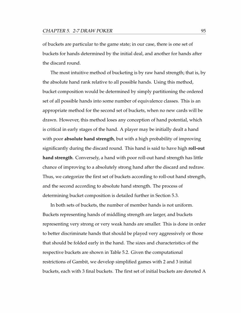
CHAPTER 5. 2-7 DRAW POKER 95
of buckets are particular to the game state; in our case, there is one set of
buckets for hands determined by the initial deal, and another for hands after
the discard round.
The most intuitive method of bucketing is by raw hand strength; that is, by
the absolute hand rank relative to all possible hands. Using this method,
bucket composition would be determined by simply partitioning the ordered
set of all possible hands into some number of equivalence classes. This is an
appropriate method for the second set of buckets, when no new cards will be
drawn. However, this method loses any conception of hand potential, which
is critical in early stages of the hand. A player may be initially dealt a hand
with poor absolute hand strength, but with a high probability of improving
significantly during the discard round. This hand is said to have high roll-out
hand strength. Conversely, a hand with poor roll-out hand strength has little
chance of improving to a absolutely strong hand after the discard and redraw.
Thus, we categorize the first set of buckets according to roll-out hand strength,
and the second according to absolute hand strength. The process of
determining bucket composition is detailed further in Section 5.3.
In both sets of buckets, the number of member hands is not uniform.
Buckets representing hands of middling strength are larger, and buckets
representing very strong or very weak hands are smaller. This is done in order
to better discriminate hands that should be played very aggressively or those
that should be folded early in the hand. The sizes and characteristics of the
respective buckets are shown in Table 5.2. Given the computational
restrictions of Gambit, we develop simplified games with 2 and 3 initial
buckets, each with 3 final buckets. The first set of initial buckets are denoted A
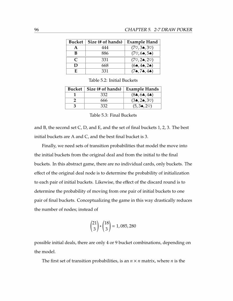
96 CHAPTER 5. 2-7 DRAW POKER
Bucket Size (# of hands) Example HandA 444 (7♥, 3♠, 3♥)B 886 (7♥, 6♠, 5♠)C 331 (7♥, 2♠, 2♥)D 668 (6♠, 4♠, 2♠)E 331 (7♠, 7♣, 4♣)
Table 5.2: Initial Buckets
Bucket Size (# of hands) Example Hands1 332 (8♣, 6♣, 4♣)2 666 (3♣, 2♠, 3♥)3 332 (5, 3♠, 2♥)
Table 5.3: Final Buckets
and B, the second set C, D, and E, and the set of final buckets 1, 2, 3. The best
initial buckets are A and C, and the best final bucket is 3.
Finally, we need sets of transition probabilities that model the move into
the initial buckets from the original deal and from the initial to the final
buckets. In this abstract game, there are no individual cards, only buckets. The
effect of the original deal node is to determine the probability of initialization
to each pair of initial buckets. Likewise, the effect of the discard round is to
determine the probability of moving from one pair of initial buckets to one
pair of final buckets. Conceptualizing the game in this way drastically reduces
the number of nodes; instead of
(213
)∗
(183
)= 1, 085, 280
possible initial deals, there are only 4 or 9 bucket combinations, depending on
the model.
The first set of transition probabilities, is an n × n matrix, where n is the
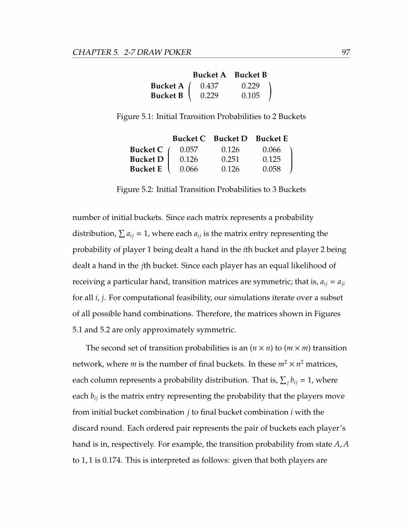
CHAPTER 5. 2-7 DRAW POKER 97
( Bucket A Bucket BBucket A 0.437 0.229Bucket B 0.229 0.105
)Figure 5.1: Initial Transition Probabilities to 2 Buckets
Bucket C Bucket D Bucket E
Bucket C 0.057 0.126 0.066Bucket D 0.126 0.251 0.125Bucket E 0.066 0.126 0.058
Figure 5.2: Initial Transition Probabilities to 3 Buckets
number of initial buckets. Since each matrix represents a probability
distribution,∑
ai j = 1, where each ai j is the matrix entry representing the
probability of player 1 being dealt a hand in the ith bucket and player 2 being
dealt a hand in the jth bucket. Since each player has an equal likelihood of
receiving a particular hand, transition matrices are symmetric; that is, ai j = a ji
for all i, j. For computational feasibility, our simulations iterate over a subset
of all possible hand combinations. Therefore, the matrices shown in Figures
5.1 and 5.2 are only approximately symmetric.
The second set of transition probabilities is an (n × n) to (m ×m) transition
network, where m is the number of final buckets. In these m2× n2 matrices,
each column represents a probability distribution. That is,∑
j bi j = 1, where
each bi j is the matrix entry representing the probability that the players move
from initial bucket combination j to final bucket combination i with the
discard round. Each ordered pair represents the pair of buckets each player’s
hand is in, respectively. For example, the transition probability from state A,A
to 1, 1 is 0.174. This is interpreted as follows: given that both players are
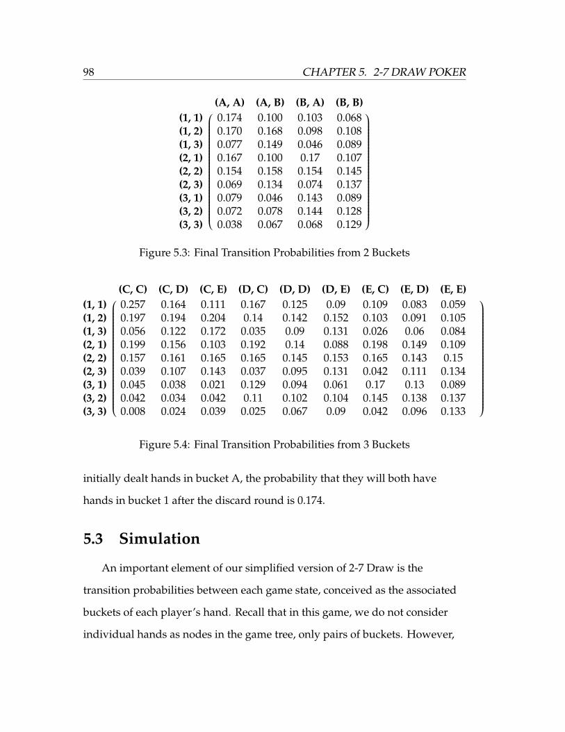
98 CHAPTER 5. 2-7 DRAW POKER
(A, A) (A, B) (B, A) (B, B)(1, 1) 0.174 0.100 0.103 0.068(1, 2) 0.170 0.168 0.098 0.108(1, 3) 0.077 0.149 0.046 0.089(2, 1) 0.167 0.100 0.17 0.107(2, 2) 0.154 0.158 0.154 0.145(2, 3) 0.069 0.134 0.074 0.137(3, 1) 0.079 0.046 0.143 0.089(3, 2) 0.072 0.078 0.144 0.128(3, 3) 0.038 0.067 0.068 0.129
Figure 5.3: Final Transition Probabilities from 2 Buckets
(C, C) (C, D) (C, E) (D, C) (D, D) (D, E) (E, C) (E, D) (E, E)(1, 1) 0.257 0.164 0.111 0.167 0.125 0.09 0.109 0.083 0.059(1, 2) 0.197 0.194 0.204 0.14 0.142 0.152 0.103 0.091 0.105(1, 3) 0.056 0.122 0.172 0.035 0.09 0.131 0.026 0.06 0.084(2, 1) 0.199 0.156 0.103 0.192 0.14 0.088 0.198 0.149 0.109(2, 2) 0.157 0.161 0.165 0.165 0.145 0.153 0.165 0.143 0.15(2, 3) 0.039 0.107 0.143 0.037 0.095 0.131 0.042 0.111 0.134(3, 1) 0.045 0.038 0.021 0.129 0.094 0.061 0.17 0.13 0.089(3, 2) 0.042 0.034 0.042 0.11 0.102 0.104 0.145 0.138 0.137(3, 3) 0.008 0.024 0.039 0.025 0.067 0.09 0.042 0.096 0.133
Figure 5.4: Final Transition Probabilities from 3 Buckets
initially dealt hands in bucket A, the probability that they will both have
hands in bucket 1 after the discard round is 0.174.
5.3 Simulation
An important element of our simplified version of 2-7 Draw is the
transition probabilities between each game state, conceived as the associated
buckets of each player’s hand. Recall that in this game, we do not consider
individual hands as nodes in the game tree, only pairs of buckets. However,
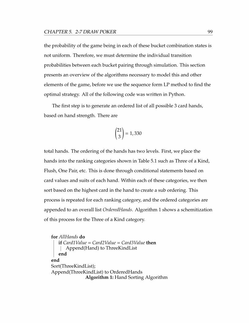
CHAPTER 5. 2-7 DRAW POKER 99
the probability of the game being in each of these bucket combination states is
not uniform. Therefore, we must determine the individual transition
probabilities between each bucket pairing through simulation. This section
presents an overview of the algorithms necessary to model this and other
elements of the game, before we use the sequence form LP method to find the
optimal strategy. All of the following code was written in Python.
The first step is to generate an ordered list of all possible 3 card hands,
based on hand strength. There are
(213
)= 1, 330
total hands. The ordering of the hands has two levels. First, we place the
hands into the ranking categories shown in Table 5.1 such as Three of a Kind,
Flush, One Pair, etc. This is done through conditional statements based on
card values and suits of each hand. Within each of these categories, we then
sort based on the highest card in the hand to create a sub ordering. This
process is repeated for each ranking category, and the ordered categories are
appended to an overall list OrderedHands. Algorithm 1 shows a schemitization
of this process for the Three of a Kind category.
for AllHands doif Card1Value = Card2Value = Card3Value then
Append(Hand) to ThreeKindListend
endSort(ThreeKindList);Append(ThreeKindList) to OrderedHands
Algorithm 1: Hand Sorting Algorithm

100 CHAPTER 5. 2-7 DRAW POKER
Recall that the particular hand composition of our initial buckets is based
on the roll-out strength of each hand, given all possible draw possibilities. We
iterate each hand over all possible draws and determine the average final hand
ranking, based on its index in OrderedHands. In order to determine which card
to discard, we use the following rule: if their hand is a pair or three of a kind,
discard one those cards. Otherwise, discard the highest card in the hand.
A general version of this process is shown in Algorithm 2. First, we
remove each of the three cards in the original hand from the available Deck,
since players cannot redraw a card that they discard. Then, if the original
hand is a Pair or Three of a Kind (PairsThreeKind), that card is replaced with
one from the Deck. Otherwise, the highest card is replaced with one from the
Deck. We then find the Strength of the new hand, given by its index in the
OrderedHands. This process iterates for each of the 18 possible cards to be
drawn. Then, for each hand, we compute the average Strength and place the
hand into a bucket with similar Strength values.
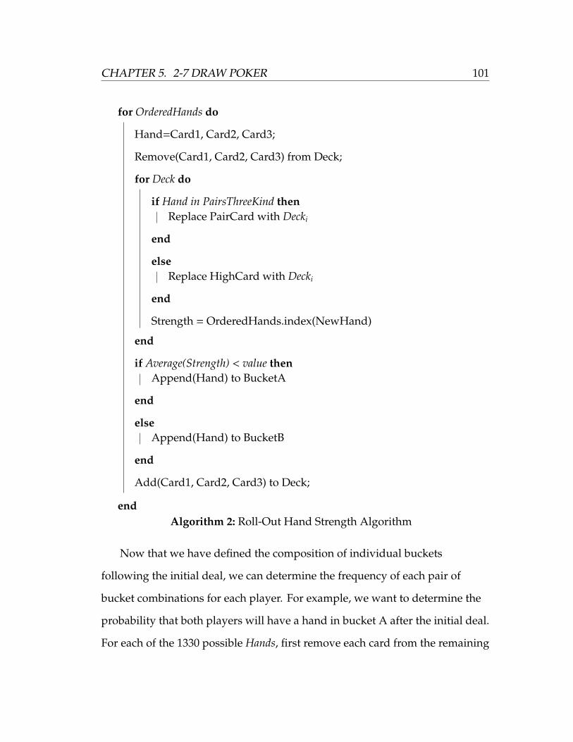
CHAPTER 5. 2-7 DRAW POKER 101
for OrderedHands do
Hand=Card1, Card2, Card3;
Remove(Card1, Card2, Card3) from Deck;
for Deck do
if Hand in PairsThreeKind thenReplace PairCard with Decki
end
elseReplace HighCard with Decki
end
Strength = OrderedHands.index(NewHand)
end
if Average(Strength) < value thenAppend(Hand) to BucketA
end
elseAppend(Hand) to BucketB
end
Add(Card1, Card2, Card3) to Deck;
endAlgorithm 2: Roll-Out Hand Strength Algorithm
Now that we have defined the composition of individual buckets
following the initial deal, we can determine the frequency of each pair of
bucket combinations for each player. For example, we want to determine the
probability that both players will have a hand in bucket A after the initial deal.
For each of the 1330 possible Hands, first remove each card from the remaining
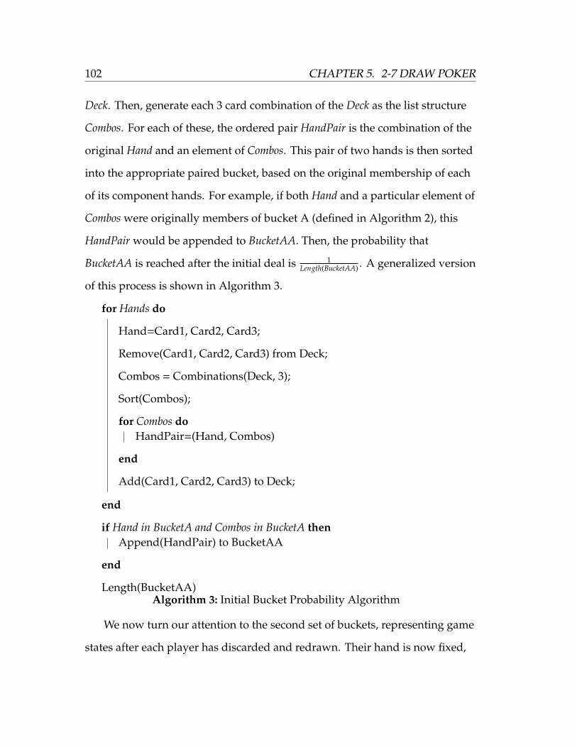
102 CHAPTER 5. 2-7 DRAW POKER
Deck. Then, generate each 3 card combination of the Deck as the list structure
Combos. For each of these, the ordered pair HandPair is the combination of the
original Hand and an element of Combos. This pair of two hands is then sorted
into the appropriate paired bucket, based on the original membership of each
of its component hands. For example, if both Hand and a particular element of
Combos were originally members of bucket A (defined in Algorithm 2), this
HandPair would be appended to BucketAA. Then, the probability that
BucketAA is reached after the initial deal is 1Length(BucketAA) . A generalized version
of this process is shown in Algorithm 3.
for Hands do
Hand=Card1, Card2, Card3;
Remove(Card1, Card2, Card3) from Deck;
Combos = Combinations(Deck, 3);
Sort(Combos);
for Combos doHandPair=(Hand, Combos)
end
Add(Card1, Card2, Card3) to Deck;
end
if Hand in BucketA and Combos in BucketA thenAppend(HandPair) to BucketAA
end
Length(BucketAA)Algorithm 3: Initial Bucket Probability Algorithm
We now turn our attention to the second set of buckets, representing game
states after each player has discarded and redrawn. Their hand is now fixed,
CHAPTER 5. 2-7 DRAW POKER 103
and we can consider a new set of buckets based only on the strength of their
hand. These buckets are defined in Table 5.3, and we define these in our code
by iterating over all 1, 085, 280 two-player hand combinations and sorting
based on the respective indices in OrderedHands. The result is a set of 9 list
structures, Bucket11, Bucket12, etc, which contain pairs of hands meeting the
criteria for each single hand bucket. For example, if both players held a hand
in the top 25% of overall hands, it would be placed in Bucket33.
With this second set of buckets defined, we now determine the transition
probabilities for moving between each first round bucket pair (defined in
Algorithm 2) and each second round bucket pair. This is the most
computationally intensive step of this simulation process, and required
time-saving measures at multiple points. This algorithm is shown in
generalized form in Algorithm 4 First, we initialize a counter Count11,
representing the number of hand pairs that fall into Bucket11. For each hand
pair in BucketAA, remove each of the six cards that one of the players holds
from the available Deck. Then, generate all permutations of Deck of length 2.
This is an ordered pair representing the cards that each player will receive
after they discard one card, respectively. For computational efficiency,
randomly select one of these and assign it to Draw. Then, replace one card in
each player’s hand with one of the cards in Draw. The particular card to be
replaced is determined by the same discard rule: if holding One Pair or Three
of a Kind, discard one of those cards. Otherwise, discard the highest card.
With the resulting pair of hands, check the membership of each in the
previously defined final buckets and increment the corresponding counter.
For example, if the both of the hands are in the strongest category in Bucket11
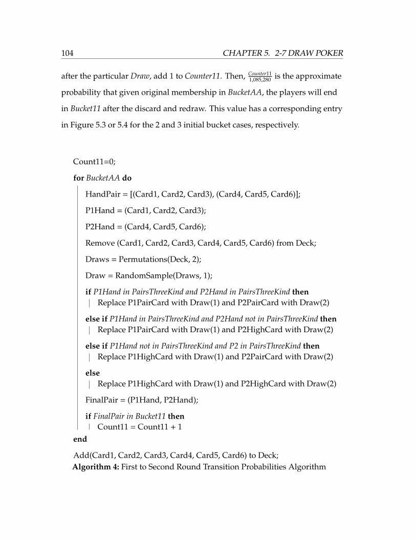
104 CHAPTER 5. 2-7 DRAW POKER
after the particular Draw, add 1 to Counter11. Then, Counter111,085,280 is the approximate
probability that given original membership in BucketAA, the players will end
in Bucket11 after the discard and redraw. This value has a corresponding entry
in Figure 5.3 or 5.4 for the 2 and 3 initial bucket cases, respectively.
Count11=0;
for BucketAA do
HandPair = [(Card1, Card2, Card3), (Card4, Card5, Card6)];
P1Hand = (Card1, Card2, Card3);
P2Hand = (Card4, Card5, Card6);
Remove (Card1, Card2, Card3, Card4, Card5, Card6) from Deck;
Draws = Permutations(Deck, 2);
Draw = RandomSample(Draws, 1);
if P1Hand in PairsThreeKind and P2Hand in PairsThreeKind thenReplace P1PairCard with Draw(1) and P2PairCard with Draw(2)
else if P1Hand in PairsThreeKind and P2Hand not in PairsThreeKind thenReplace P1PairCard with Draw(1) and P2HighCard with Draw(2)
else if P1Hand not in PairsThreeKind and P2 in PairsThreeKind thenReplace P1HighCard with Draw(1) and P2PairCard with Draw(2)
elseReplace P1HighCard with Draw(1) and P2HighCard with Draw(2)
FinalPair = (P1Hand, P2Hand);
if FinalPair in Bucket11 thenCount11 = Count11 + 1
end
Add(Card1, Card2, Card3, Card4, Card5, Card6) to Deck;Algorithm 4: First to Second Round Transition Probabilities Algorithm
CHAPTER 5. 2-7 DRAW POKER 105
5.4 Results
We solve the sequence form LP of Simplified 2-7 Draw using the Gambit
software package, for both the 2 and 3 initial bucket cases. The solutions to
these LPs are the optimal realization plans for each game. These LPs also
compute an expected value of the game, which is simply the optimal objective
function value. Gambit’s sequence form LP algorithms compute only one
optimal solution; there may be other optimal realization plans for Simplified
2-7 Draw. This section provides a brief discussion of Gambit’s computed
solution; for more detail, see Appendix B.
5.4.1 2 Initial Buckets
For the 2 initial bucket case, both player’s optimal realization plans
characterize a relatively conservative strategy. We begin by discussing player
1’s optimal play. Player 1 is first dealt a random hand, which is a member of
either Bucket A or Bucket B. Hands in Bucket A have a higher average roll-out
hand strength than hands in Bucket B. On his first opportunity to bet, player 1
should always check. If player 2 bets after player 1 checks, player 1 should
always call the bet. Thus, player 1’s strategy for the first round is simple:
regardless of Bucket, check and call a bet if necessary.
After the first round of betting, each player discards and redraws one card
from the remaining deck. At this point, player 1’s optimal realization plan
becomes more complicated. It defines optimal play for each combination of
original bucket and final bucket. Recall that in the final round, hands are
sorted by absolute strength into Buckets 1 − 3, in ascending order. Hands in
106 CHAPTER 5. 2-7 DRAW POKER
Bucket 3 are superior to those in Bucket 2, which are in turn superior to those
in Bucket 1. If player 1’s hand was originally in Bucket A and both players
checked in the first betting round, he should bet with probability 0.178 while
holding a hand in Bucket 1, always check with Bucket 2, and always bet with
Bucket 3. If he does check and player 2 then bets, player 1 should always fold
with Bucket 1 and always call with Bucket 2. Notice that this optimal
realization plan does not specify what player 1 should do with a hand in
Bucket 3 after player 2 has bet; since it is optimal for player 1 to always bet
with Bucket 1 initially, he will simply never be in this situation. These
irrelevant sequences are denoted *** in the full table of results in Appendix B.
If player 1’s hand was originally in Bucket A and the betting sequence of
the first round was player 1 checks, player 2 bets, and player 1 calls, player 1
should bet with probability 0.122 while holding a hand in Bucket 1, always
check with Bucket 2, and always bet with Bucket 3. If player 1 checks and
player 2 bets, player 1 should always fold with Bucket 1 and always call with
Bucket 2. If player 1’s hand was originally in Bucket B and both player’s
checked in the first round, player 1 should always check with Bucket 1, bet
with probability 0.233 with Bucket 2, and always bet with Bucket 3. If player 1
checks and player 2 bets, always fold with Bucket 1 and call with Bucket 2. If
player 1’s hand was originally in Bucket B and the betting sequence of the first
round was player 1 checks, player 2 bets, and player 1 calls, player 1 should
always bet with Bucket 1, check with Bucket 2, and always bet with Bucket 3.
If player 1 checks and player 2 bets, always call with Bucket 2.
Player 2’s first round strategy is more aggressive and complex than player
1’s. If player 1 checks, player 2 should always check with Bucket A and always
CHAPTER 5. 2-7 DRAW POKER 107
bet with Bucket B. If player 1 bets, player 2 should call with probability 0.983
with Bucket A and always call with Bucket B. The discard and redraw follows
this round of betting. If player 2 originally had a hand in Bucket A and both
players checked in the first round, and player 1 bets in the final round, player
2 should always fold with Bucket 1, call with probability 0.891 with Bucket 2,
and always call with Bucket 3. Since player 2 never checks in the first round
with Bucket B, we need not define a realization plan for the second round.
If player 2 originally had a hand in Bucket B, the first round betting action
was player 1 checks, player 2 bets, and player 1 calls, and player 1 checks after
the discard and redraw, player 2 should always bet with Bucket 1, bet with
probability 0.435 with Bucket 2, and always bet with Bucket 3. Instead, if
player 1 bets, player 2 should call with probability 0.415 with Bucket 1, and
always call with Buckets 2 and 3.
If player 2 originally had a hand in Bucket A, the first round betting action
was player 1 bets and player 2 calls, and player 1 bets after the discard and
redraw, player 2 should call with probability 0.664 with Bucket 1, always with
Bucket 2, and with probability 0.640 with Bucket 3. If player 1 checks, player 2
should always check with every Bucket. If player 2 instead originally had a
hand in Bucket B, he should always call with Buckets 1 and 2, and with
probability 0.595 with Bucket 3. If player 1 checks, player 2 should always
check with every Bucket.
When each player uses these optimal realization plans, the value of the
game is approximately − 14100 . This value is from player 1’s perspective; for each
hand of Simplified 2-7 Draw played according to these optimal realization
plans, player 1 can expected to lose 14100 betting units to player 2. Recall that the
108 CHAPTER 5. 2-7 DRAW POKER
value of optimally-played Kuhn Poker is − 118 . In Simplified 2-7 Draw, player 2
has an even greater advantage than in Kuhn Poker. This is likely due to an
even greater positional advantage; player 2 acts second on two rounds of
betting, instead of only one. In each round, player 2 can observe player 1’s
actions before making his own decision.
Some parts of these optimal realization probabilities are surprising, while
others square with previous intuition about poker strategy. The most
surprising results are player 2’s optimal probabilities in the final betting
round, after a first round in which the betting action was player 1 bets and
player 2 calls. In this situation, the LP results dictate that player 2 should
sometimes fold while facing a bet and always check back while holding a
hand in Bucket 3. This is extremely suprising; since Bucket 3 is the strongest
possible bucket, player 2 can never outright lose the hand. Therefore, we
would expect that he should want to bet as much as possible. The reason for
this prescribed strategy is not clear; it may be a coding error or an inherent
issue related to the structure of the game.
However, the majority of these optimal realization plans are congruent
with our intuitive sense of poker strategy. For example, player 1 consistently
folds a poor hand from Bucket 1 and calls a strong hand from Bucket 3 when
facing a bet in the final round. For the most part, each player follows a
strategy of betting with a combination of bluffs (Bucket 1) and strong hands
(Bucket 3). In addition, they often call with medium strength hands (Bucket 2),
hoping that their opponent is bluffing. These strategies are similar to those in
Kuhn Poker; Buckets 1,2, and 3 play similarly to a Jack, Queen, and King,
respectively.
CHAPTER 5. 2-7 DRAW POKER 109
Finally, it is notable that little folding should occur in the first betting
round. Player 2 folds with probability 0.017 when holding a hand in Bucket A
when player 1 bets. Otherwise, each player’s optimal realization plan involves
always remaining in the hand until the final betting round. This highlights the
importance of the discard and redraw phase, where each player’s hand
strength can change dramatically. Each initial buckets contained plenty of
hands that could become very strong after the discard and redraw; this was
simply more likely with Bucket A. This feature illustrates a considerable issue
with the abstraction techniques that we used to reduce 2-7 Draw to a tractable
size. It is likely that more specific buckets, a bigger deck, bigger individual
hands, and more betting rounds would incentivize players to fold more often
before the final betting round.
5.4.2 3 Initial Buckets
We hypothesized that a different version of Simplified 2-7 Draw with an
additional bucket in the first betting round would provide a more robust set of
initial betting strategies. However, the computational limits of the Gambit
software package made this difficult. When solving a sequence form LP,
Gambit allows the user to specify computation using rational or non-rational
values. The rational method is more accurate, but the computation time
required is much greater. One of Gambit’s developers notes that the use of
floating point arithmetic can lead to numerical instability, and strongly
recommends using the rational algorithm [11].
We initially attempted to solve our 3 initial bucket model using the
rational method; after 4 days, the program did not output a solution. It is not
110 CHAPTER 5. 2-7 DRAW POKER
clear how long a game of this size would take to run, but we were surprised
that the algorithm could not finish. The 2 initial bucket LP with 80 information
sets computed a solution rationally within 20 minutes, and the 3 initial bucket
LP only has 120 information sets. Fortunately, the non-rational algorithm for
the 3 initial bucket LP finishes within an hour. However, these results are
clearly flawed, and are shown in Appendix B. Many of the supposed optimal
probabilities cannot even be such; they often do not sum to 1 in each
information set, are negative, or are greater than 1. We report these results for
the sake of completeness of the project, but they cannot accurately describe an
optimal realization plan for the game. Future versions of Gambit and more
powerful computers may be able to find the exact rational solution.
Chapter 6
Conclusion
This Independent Study is an exposition of the use of linear programming
and game theoretic techniques to find optimal poker strategies. Game theory
represents games in a variety of forms, some of which can be used to find the
Nash equilibrium strategies using linear programming techniques. In
particular, we used the sequence form representation to find Nash-optimal
strategies for Kuhn Poker and a novel, simplified version of 2-7 Draw. The
Gambit software package was a critical tool, in both constructing and solving
the sequence form LPs. The particular optimal strategies for Simplified 2-7
Draw are less robust than we hoped; they prescribe a relatively simple
strategy for both players. These strategies may not be particularly applicable
to the actual game of 2-7 Draw, given the degree of abstraction and
simplification necessary in our model.
These results could be extended in several ways. For example, we could
consider a version of Simplified 2-7 Draw that uses more buckets, more
rounds of betting, or more cards. Any of the abstraction techniques presented
111

112 CHAPTER 6. CONCLUSION
in Section 5.2.2 could be modified to create a more realistic game. While our
version is a reasonable approximation, it loses many key facets of the game.
For example, players are not actually required to discard and redraw a card at
every opportunity, nor by our specific discard rule. Thus, a natural extension
of this project is to analyze a version with fewer abstractions.
Computational constraints played a significant role in our analysis of
Simplified 2-7 Draw, and considering a more accurate version would require
better computational tools. The current version of Gambit can compute
solutions for medium-sized games like ours, but quickly fails when faced with
truly large-scale games. The current version of Gambit is unable to find
optimal strategies of large games using the sequence form LP method, but
may be able to using other methods. Although not discussed or utilized in this
project, Gambit does have a variety of other methods of finding optimal
strategies [6]. Building the sequence form LPs manually, instead of
automatically with Gambit, would be difficult and prone to error. However,
they could be solved using external solvers, which are much more able to
handle large LPs. For example, a sequence form LP with over 1.1 million
variables was used to solve an abstracted game of Rhode Island Hold’Em with
external LP solvers [9]. Future work based on computational improvement
could use a more advanced version of Gambit, a different solution method, or
external LP solvers.
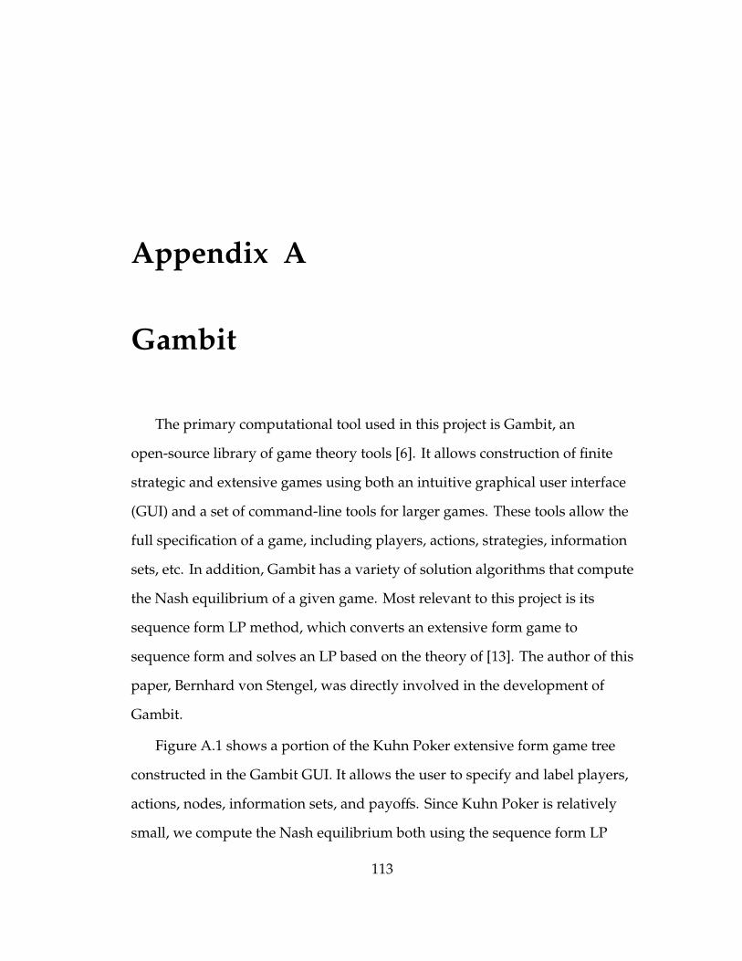
Appendix A
Gambit
The primary computational tool used in this project is Gambit, an
open-source library of game theory tools [6]. It allows construction of finite
strategic and extensive games using both an intuitive graphical user interface
(GUI) and a set of command-line tools for larger games. These tools allow the
full specification of a game, including players, actions, strategies, information
sets, etc. In addition, Gambit has a variety of solution algorithms that compute
the Nash equilibrium of a given game. Most relevant to this project is its
sequence form LP method, which converts an extensive form game to
sequence form and solves an LP based on the theory of [13]. The author of this
paper, Bernhard von Stengel, was directly involved in the development of
Gambit.
Figure A.1 shows a portion of the Kuhn Poker extensive form game tree
constructed in the Gambit GUI. It allows the user to specify and label players,
actions, nodes, information sets, and payoffs. Since Kuhn Poker is relatively
small, we compute the Nash equilibrium both using the sequence form LP
113
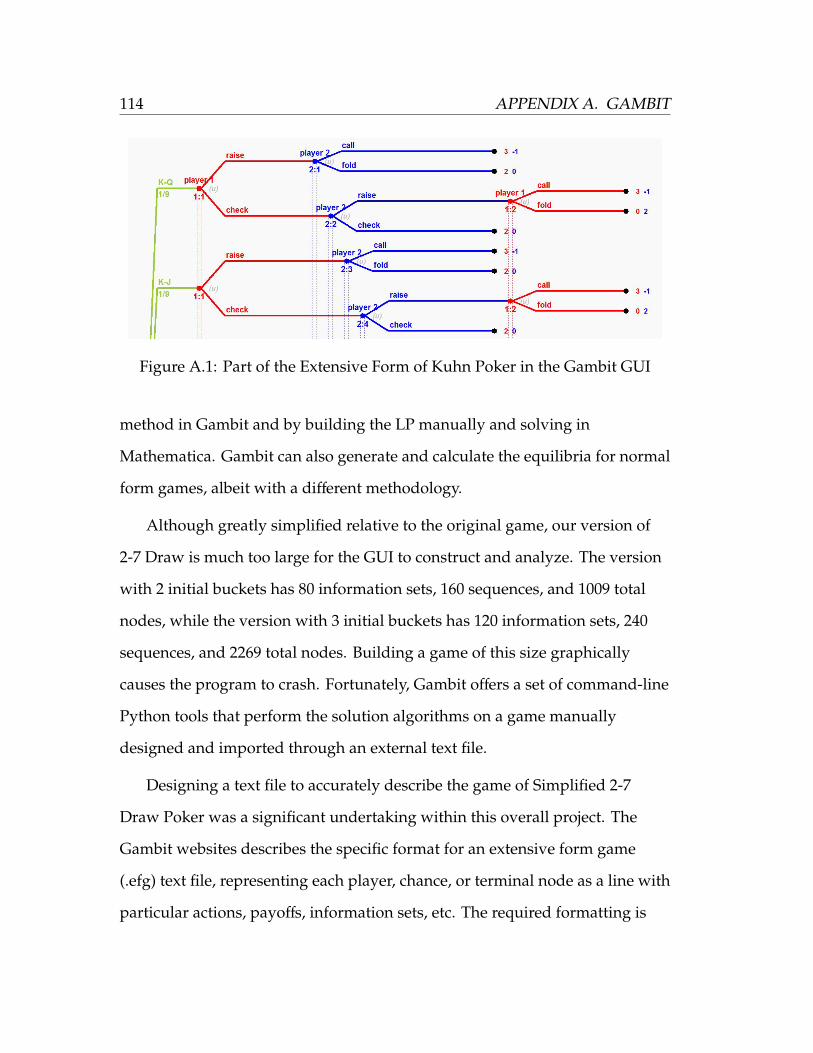
114 APPENDIX A. GAMBIT
Figure A.1: Part of the Extensive Form of Kuhn Poker in the Gambit GUI
method in Gambit and by building the LP manually and solving in
Mathematica. Gambit can also generate and calculate the equilibria for normal
form games, albeit with a different methodology.
Although greatly simplified relative to the original game, our version of
2-7 Draw is much too large for the GUI to construct and analyze. The version
with 2 initial buckets has 80 information sets, 160 sequences, and 1009 total
nodes, while the version with 3 initial buckets has 120 information sets, 240
sequences, and 2269 total nodes. Building a game of this size graphically
causes the program to crash. Fortunately, Gambit offers a set of command-line
Python tools that perform the solution algorithms on a game manually
designed and imported through an external text file.
Designing a text file to accurately describe the game of Simplified 2-7
Draw Poker was a significant undertaking within this overall project. The
Gambit websites describes the specific format for an extensive form game
(.efg) text file, representing each player, chance, or terminal node as a line with
particular actions, payoffs, information sets, etc. The required formatting is
APPENDIX A. GAMBIT 115
very specific, and is described in more detail on Gambit’s website. To generate
this .efg text file, we utilize an original Python script that utilizes several types
of symmetry present in the game tree. Since the betting structure is uniform
across different bucket combinations, appropriate for loops can be used to
iterate over the entire game tree. These files also specify the transition
probabilities for each chance node, as detailed in Sections 5.2.3 and 5.3. These
scripts are developed for both the 2 and 3 initial bucket cases. The results of
the scripts are text files that are 1135 and 2550 lines, respectively.
These text files are then imported to an installed Python environment
containing Gambit’s solver algorithms and other commands. The
gambit.nash.lp solve() command generates and solves the sequence form LP
and returns complete Nash-optimal behavior strategies for each sequence. For
many of the information sets, optimal play dictates taking a particular action
with probability 1. For any such information set, sequences later in the game
that require the other action are reported as being played with the default
probability 0.5. For example, the optimal strategy in the 2 initial bucket case
includes always checking in the first betting round as player 1. Consequently,
any sequence in the second betting round that involves player 1 previously
betting in the first betting round are reported as 0.5. Since these later
information sets will never be reached, these values are irrelevant in our
analysis.
The first version of Simplified 2-7 Triple Draw that we developed involved
combinations of 5 buckets for the first round of betting, transitioning to
combinations of 3 buckets for the second round. This is in contrast to the 2 and
3 initial bucket versions for which we present solutions in Chapter 5. The 5
116 APPENDIX A. GAMBIT
bucket case is more complex, with 200 information sets, 400 sequences, and
6301 nodes. Attempts to find a Nash equilibrium for this game with Gambit
return an unexplained error. Direct correspondence with Gambit developer
Theodore Turocy suggests that a solving a game of this size is infeasible in
Gambit’s current version [11].
Appendix B
Simplified 2-7 Draw LP Results
The following tables show the results of the Simplified 2-7 Draw sequence
form LPs. Each row denotes an information set for a particular player, each of
which has two possible actions. The Information column denotes the
previous action and information known to the player; this describes the
information set. The P(C/F) column lists the probability that the optimal
player should check or fold, depending on context. The P(B/C column lists the
corresponding probability that of the other action, either betting or calling. For
example, information set 1 for player 1 prescribes checking with probability
0.822 and betting with probability 0.178, given that player 1 initially had a
hand in Bucket 1, then both players checked, and now he has a hand in Bucket
1. Many of the information sets with ‘optimal‘ probabilities of 0.5 for each
action is a history that the player will never face, given the other prescriptions
of strategy. For example, consider information set 14 for player 1. In the
associated history, player 1 bet after the initial deal; since he always checks in
the situation per information set 0, he will never face the choice of actions in
117
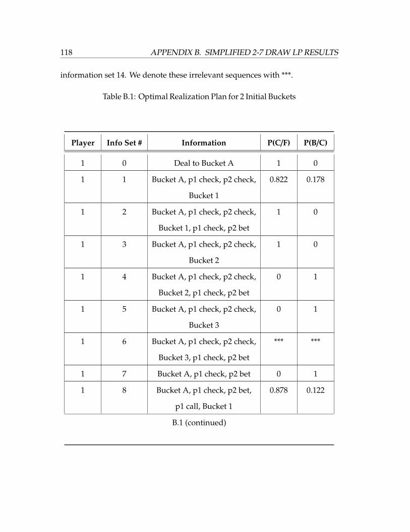
118 APPENDIX B. SIMPLIFIED 2-7 DRAW LP RESULTS
information set 14. We denote these irrelevant sequences with ***.
Table B.1: Optimal Realization Plan for 2 Initial Buckets
Player Info Set # Information P(C/F) P(B/C)
1 0 Deal to Bucket A 1 0
1 1 Bucket A, p1 check, p2 check,
Bucket 1
0.822 0.178
1 2 Bucket A, p1 check, p2 check,
Bucket 1, p1 check, p2 bet
1 0
1 3 Bucket A, p1 check, p2 check,
Bucket 2
1 0
1 4 Bucket A, p1 check, p2 check,
Bucket 2, p1 check, p2 bet
0 1
1 5 Bucket A, p1 check, p2 check,
Bucket 3
0 1
1 6 Bucket A, p1 check, p2 check,
Bucket 3, p1 check, p2 bet
*** ***
1 7 Bucket A, p1 check, p2 bet 0 1
1 8 Bucket A, p1 check, p2 bet,
p1 call, Bucket 1
0.878 0.122
B.1 (continued)
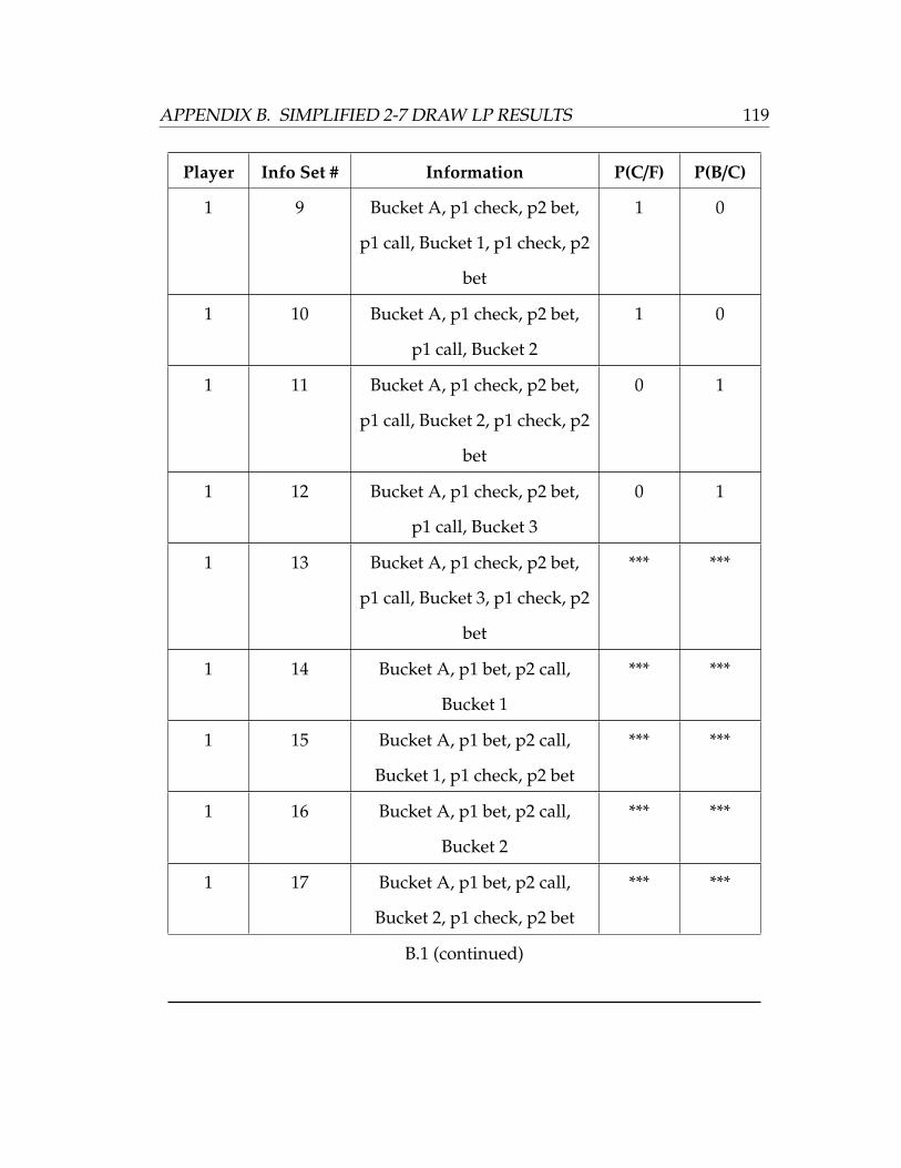
APPENDIX B. SIMPLIFIED 2-7 DRAW LP RESULTS 119
Player Info Set # Information P(C/F) P(B/C)
1 9 Bucket A, p1 check, p2 bet,
p1 call, Bucket 1, p1 check, p2
bet
1 0
1 10 Bucket A, p1 check, p2 bet,
p1 call, Bucket 2
1 0
1 11 Bucket A, p1 check, p2 bet,
p1 call, Bucket 2, p1 check, p2
bet
0 1
1 12 Bucket A, p1 check, p2 bet,
p1 call, Bucket 3
0 1
1 13 Bucket A, p1 check, p2 bet,
p1 call, Bucket 3, p1 check, p2
bet
*** ***
1 14 Bucket A, p1 bet, p2 call,
Bucket 1
*** ***
1 15 Bucket A, p1 bet, p2 call,
Bucket 1, p1 check, p2 bet
*** ***
1 16 Bucket A, p1 bet, p2 call,
Bucket 2
*** ***
1 17 Bucket A, p1 bet, p2 call,
Bucket 2, p1 check, p2 bet
*** ***
B.1 (continued)
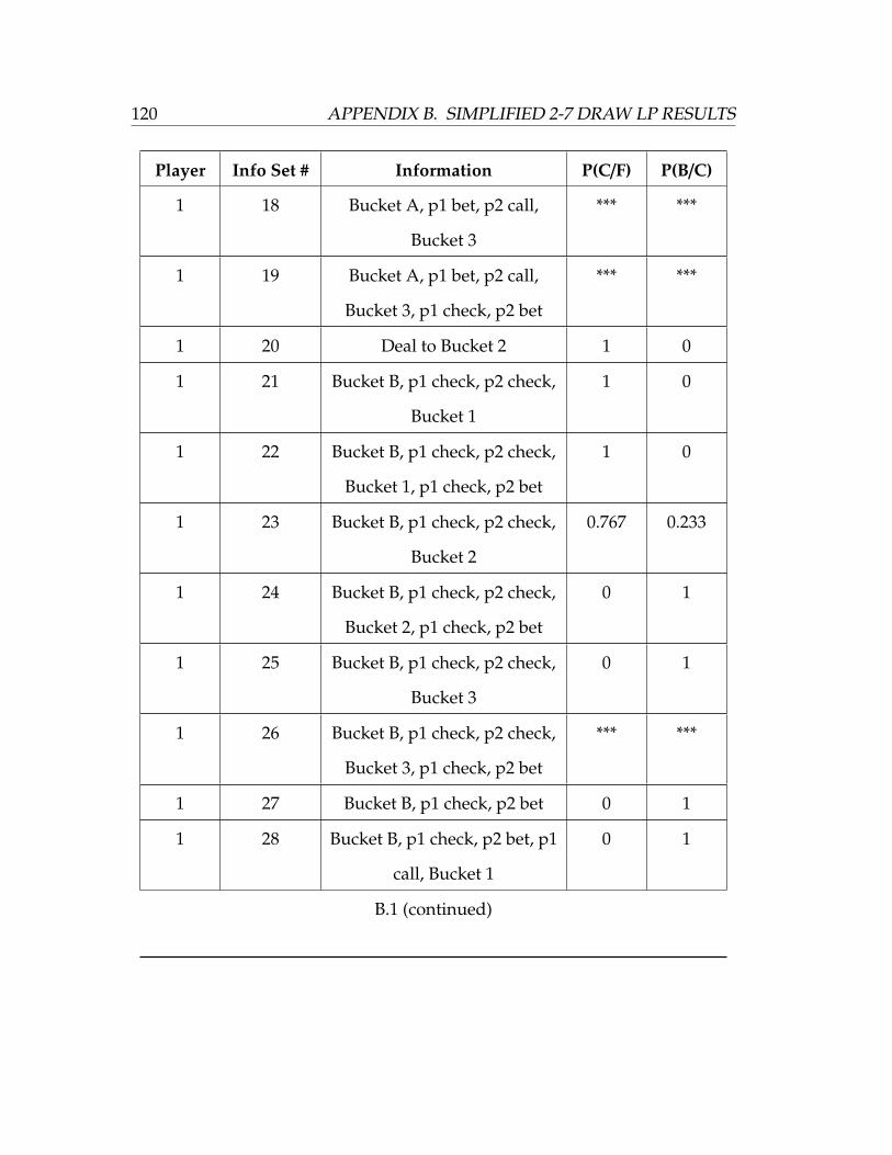
120 APPENDIX B. SIMPLIFIED 2-7 DRAW LP RESULTS
Player Info Set # Information P(C/F) P(B/C)
1 18 Bucket A, p1 bet, p2 call,
Bucket 3
*** ***
1 19 Bucket A, p1 bet, p2 call,
Bucket 3, p1 check, p2 bet
*** ***
1 20 Deal to Bucket 2 1 0
1 21 Bucket B, p1 check, p2 check,
Bucket 1
1 0
1 22 Bucket B, p1 check, p2 check,
Bucket 1, p1 check, p2 bet
1 0
1 23 Bucket B, p1 check, p2 check,
Bucket 2
0.767 0.233
1 24 Bucket B, p1 check, p2 check,
Bucket 2, p1 check, p2 bet
0 1
1 25 Bucket B, p1 check, p2 check,
Bucket 3
0 1
1 26 Bucket B, p1 check, p2 check,
Bucket 3, p1 check, p2 bet
*** ***
1 27 Bucket B, p1 check, p2 bet 0 1
1 28 Bucket B, p1 check, p2 bet, p1
call, Bucket 1
0 1
B.1 (continued)
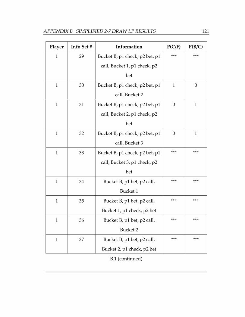
APPENDIX B. SIMPLIFIED 2-7 DRAW LP RESULTS 121
Player Info Set # Information P(C/F) P(B/C)
1 29 Bucket B, p1 check, p2 bet, p1
call, Bucket 1, p1 check, p2
bet
*** ***
1 30 Bucket B, p1 check, p2 bet, p1
call, Bucket 2
1 0
1 31 Bucket B, p1 check, p2 bet, p1
call, Bucket 2, p1 check, p2
bet
0 1
1 32 Bucket B, p1 check, p2 bet, p1
call, Bucket 3
0 1
1 33 Bucket B, p1 check, p2 bet, p1
call, Bucket 3, p1 check, p2
bet
*** ***
1 34 Bucket B, p1 bet, p2 call,
Bucket 1
*** ***
1 35 Bucket B, p1 bet, p2 call,
Bucket 1, p1 check, p2 bet
*** ***
1 36 Bucket B, p1 bet, p2 call,
Bucket 2
*** ***
1 37 Bucket B, p1 bet, p2 call,
Bucket 2, p1 check, p2 bet
*** ***
B.1 (continued)
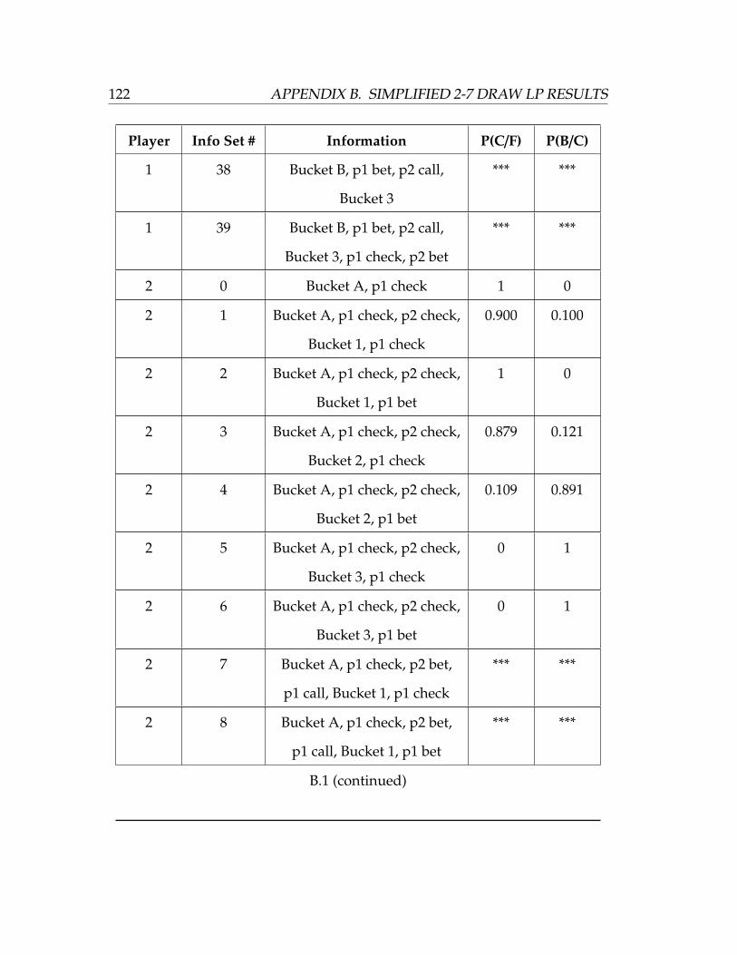
122 APPENDIX B. SIMPLIFIED 2-7 DRAW LP RESULTS
Player Info Set # Information P(C/F) P(B/C)
1 38 Bucket B, p1 bet, p2 call,
Bucket 3
*** ***
1 39 Bucket B, p1 bet, p2 call,
Bucket 3, p1 check, p2 bet
*** ***
2 0 Bucket A, p1 check 1 0
2 1 Bucket A, p1 check, p2 check,
Bucket 1, p1 check
0.900 0.100
2 2 Bucket A, p1 check, p2 check,
Bucket 1, p1 bet
1 0
2 3 Bucket A, p1 check, p2 check,
Bucket 2, p1 check
0.879 0.121
2 4 Bucket A, p1 check, p2 check,
Bucket 2, p1 bet
0.109 0.891
2 5 Bucket A, p1 check, p2 check,
Bucket 3, p1 check
0 1
2 6 Bucket A, p1 check, p2 check,
Bucket 3, p1 bet
0 1
2 7 Bucket A, p1 check, p2 bet,
p1 call, Bucket 1, p1 check
*** ***
2 8 Bucket A, p1 check, p2 bet,
p1 call, Bucket 1, p1 bet
*** ***
B.1 (continued)

APPENDIX B. SIMPLIFIED 2-7 DRAW LP RESULTS 123
Player Info Set # Information P(C/F) P(B/C)
2 9 Bucket A, p1 check, p2 bet,
p1 call, Bucket 2, p1 check
*** ***
2 10 Bucket A, p1 check, p2 bet,
p1 call, Bucket 2, p1 bet
*** ***
2 11 Bucket A, p1 check, p2 bet,
p1 call, Bucket 3, p1 check
*** ***
2 12 Bucket A, p1 check, p2 bet,
p1 call, Bucket 3, p1 bet
*** ***
2 13 Bucket A, p1 bet 0.017 0.983
2 14 Bucket A, p1 bet, p2 call,
Bucket 1, p1 check
1 0
2 15 Bucket A, p1 bet, p2 call,
Bucket 1, p1 bet
0.336 0.664
2 16 Bucket A, p1 bet, p2 call,
Bucket 2, p1 check
1 0
2 17 Bucket A, p1 bet, p2 call,
Bucket 2, p1 bet
0 1
2 18 Bucket A, p1 bet, p2 call,
Bucket 3, p1 check
1 0
2 19 Bucket A, p1 bet, p2 call,
Bucket 3, p1 bet
0.361 0.639
B.1 (continued)
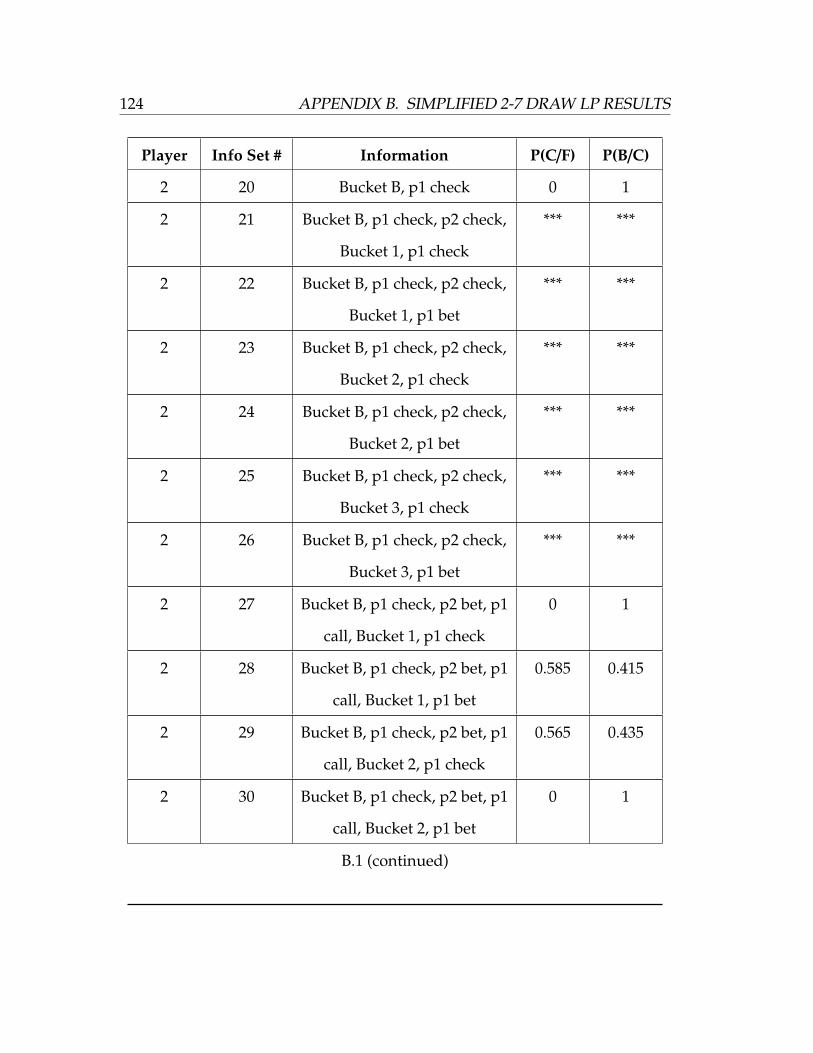
124 APPENDIX B. SIMPLIFIED 2-7 DRAW LP RESULTS
Player Info Set # Information P(C/F) P(B/C)
2 20 Bucket B, p1 check 0 1
2 21 Bucket B, p1 check, p2 check,
Bucket 1, p1 check
*** ***
2 22 Bucket B, p1 check, p2 check,
Bucket 1, p1 bet
*** ***
2 23 Bucket B, p1 check, p2 check,
Bucket 2, p1 check
*** ***
2 24 Bucket B, p1 check, p2 check,
Bucket 2, p1 bet
*** ***
2 25 Bucket B, p1 check, p2 check,
Bucket 3, p1 check
*** ***
2 26 Bucket B, p1 check, p2 check,
Bucket 3, p1 bet
*** ***
2 27 Bucket B, p1 check, p2 bet, p1
call, Bucket 1, p1 check
0 1
2 28 Bucket B, p1 check, p2 bet, p1
call, Bucket 1, p1 bet
0.585 0.415
2 29 Bucket B, p1 check, p2 bet, p1
call, Bucket 2, p1 check
0.565 0.435
2 30 Bucket B, p1 check, p2 bet, p1
call, Bucket 2, p1 bet
0 1
B.1 (continued)
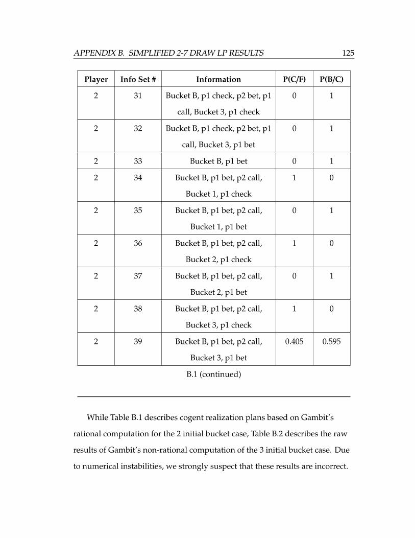
APPENDIX B. SIMPLIFIED 2-7 DRAW LP RESULTS 125
Player Info Set # Information P(C/F) P(B/C)
2 31 Bucket B, p1 check, p2 bet, p1
call, Bucket 3, p1 check
0 1
2 32 Bucket B, p1 check, p2 bet, p1
call, Bucket 3, p1 bet
0 1
2 33 Bucket B, p1 bet 0 1
2 34 Bucket B, p1 bet, p2 call,
Bucket 1, p1 check
1 0
2 35 Bucket B, p1 bet, p2 call,
Bucket 1, p1 bet
0 1
2 36 Bucket B, p1 bet, p2 call,
Bucket 2, p1 check
1 0
2 37 Bucket B, p1 bet, p2 call,
Bucket 2, p1 bet
0 1
2 38 Bucket B, p1 bet, p2 call,
Bucket 3, p1 check
1 0
2 39 Bucket B, p1 bet, p2 call,
Bucket 3, p1 bet
0.405 0.595
B.1 (continued)
While Table B.1 describes cogent realization plans based on Gambit’s
rational computation for the 2 initial bucket case, Table B.2 describes the raw
results of Gambit’s non-rational computation of the 3 initial bucket case. Due
to numerical instabilities, we strongly suspect that these results are incorrect.
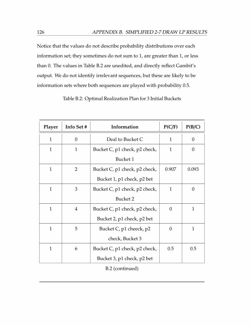
126 APPENDIX B. SIMPLIFIED 2-7 DRAW LP RESULTS
Notice that the values do not describe probability distributions over each
information set; they sometimes do not sum to 1, are greater than 1, or less
than 0. The values in Table B.2 are unedited, and directly reflect Gambit’s
output. We do not identify irrelevant sequences, but these are likely to be
information sets where both sequences are played with probability 0.5.
Table B.2: Optimal Realization Plan for 3 Initial Buckets
Player Info Set # Information P(C/F) P(B/C)
1 0 Deal to Bucket C 1 0
1 1 Bucket C, p1 check, p2 check,
Bucket 1
1 0
1 2 Bucket C, p1 check, p2 check,
Bucket 1, p1 check, p2 bet
0.907 0.093
1 3 Bucket C, p1 check, p2 check,
Bucket 2
1 0
1 4 Bucket C, p1 check, p2 check,
Bucket 2, p1 check, p2 bet
0 1
1 5 Bucket C, p1 cheeck, p2
check, Bucket 3
0 1
1 6 Bucket C, p1 check, p2 check,
Bucket 3, p1 check, p2 bet
0.5 0.5
B.2 (continued)
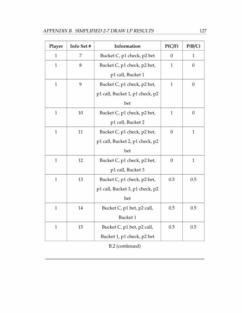
APPENDIX B. SIMPLIFIED 2-7 DRAW LP RESULTS 127
Player Info Set # Information P(C/F) P(B/C)
1 7 Bucket C, p1 check, p2 bet 0 1
1 8 Bucket C, p1 check, p2 bet,
p1 call, Bucket 1
1 0
1 9 Bucket C, p1 check, p2 bet,
p1 call, Bucket 1, p1 check, p2
bet
1 0
1 10 Bucket C, p1 check, p2 bet,
p1 call, Bucket 2
1 0
1 11 Bucket C, p1 check, p2 bet,
p1 call, Bucket 2, p1 check, p2
bet
0 1
1 12 Bucket C, p1 check, p2 bet,
p1 call, Bucket 3
0 1
1 13 Bucket C, p1 check, p2 bet,
p1 call, Bucket 3, p1 check, p2
bet
0.5 0.5
1 14 Bucket C, p1 bet, p2 call,
Bucket 1
0.5 0.5
1 15 Bucket C, p1 bet, p2 call,
Bucket 1, p1 check, p2 bet
0.5 0.5
B.2 (continued)
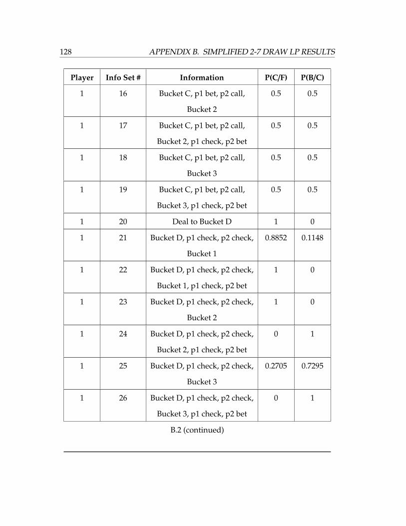
128 APPENDIX B. SIMPLIFIED 2-7 DRAW LP RESULTS
Player Info Set # Information P(C/F) P(B/C)
1 16 Bucket C, p1 bet, p2 call,
Bucket 2
0.5 0.5
1 17 Bucket C, p1 bet, p2 call,
Bucket 2, p1 check, p2 bet
0.5 0.5
1 18 Bucket C, p1 bet, p2 call,
Bucket 3
0.5 0.5
1 19 Bucket C, p1 bet, p2 call,
Bucket 3, p1 check, p2 bet
0.5 0.5
1 20 Deal to Bucket D 1 0
1 21 Bucket D, p1 check, p2 check,
Bucket 1
0.8852 0.1148
1 22 Bucket D, p1 check, p2 check,
Bucket 1, p1 check, p2 bet
1 0
1 23 Bucket D, p1 check, p2 check,
Bucket 2
1 0
1 24 Bucket D, p1 check, p2 check,
Bucket 2, p1 check, p2 bet
0 1
1 25 Bucket D, p1 check, p2 check,
Bucket 3
0.2705 0.7295
1 26 Bucket D, p1 check, p2 check,
Bucket 3, p1 check, p2 bet
0 1
B.2 (continued)
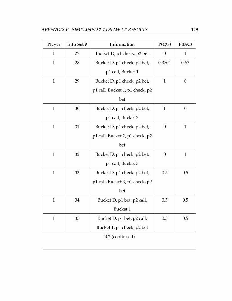
APPENDIX B. SIMPLIFIED 2-7 DRAW LP RESULTS 129
Player Info Set # Information P(C/F) P(B/C)
1 27 Bucket D, p1 check, p2 bet 0 1
1 28 Bucket D, p1 check, p2 bet,
p1 call, Bucket 1
0.3701 0.63
1 29 Bucket D, p1 check, p2 bet,
p1 call, Bucket 1, p1 check, p2
bet
1 0
1 30 Bucket D, p1 check, p2 bet,
p1 call, Bucket 2
1 0
1 31 Bucket D, p1 check, p2 bet,
p1 call, Bucket 2, p1 check, p2
bet
0 1
1 32 Bucket D, p1 check, p2 bet,
p1 call, Bucket 3
0 1
1 33 Bucket D, p1 check, p2 bet,
p1 call, Bucket 3, p1 check, p2
bet
0.5 0.5
1 34 Bucket D, p1 bet, p2 call,
Bucket 1
0.5 0.5
1 35 Bucket D, p1 bet, p2 call,
Bucket 1, p1 check, p2 bet
0.5 0.5
B.2 (continued)
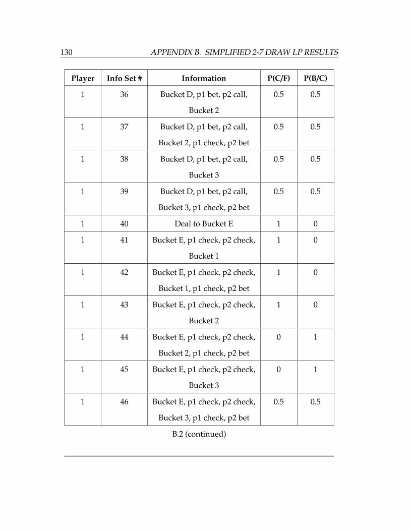
130 APPENDIX B. SIMPLIFIED 2-7 DRAW LP RESULTS
Player Info Set # Information P(C/F) P(B/C)
1 36 Bucket D, p1 bet, p2 call,
Bucket 2
0.5 0.5
1 37 Bucket D, p1 bet, p2 call,
Bucket 2, p1 check, p2 bet
0.5 0.5
1 38 Bucket D, p1 bet, p2 call,
Bucket 3
0.5 0.5
1 39 Bucket D, p1 bet, p2 call,
Bucket 3, p1 check, p2 bet
0.5 0.5
1 40 Deal to Bucket E 1 0
1 41 Bucket E, p1 check, p2 check,
Bucket 1
1 0
1 42 Bucket E, p1 check, p2 check,
Bucket 1, p1 check, p2 bet
1 0
1 43 Bucket E, p1 check, p2 check,
Bucket 2
1 0
1 44 Bucket E, p1 check, p2 check,
Bucket 2, p1 check, p2 bet
0 1
1 45 Bucket E, p1 check, p2 check,
Bucket 3
0 1
1 46 Bucket E, p1 check, p2 check,
Bucket 3, p1 check, p2 bet
0.5 0.5
B.2 (continued)

APPENDIX B. SIMPLIFIED 2-7 DRAW LP RESULTS 131
Player Info Set # Information P(C/F) P(B/C)
1 47 Bucket E, p1 check, p2 bet 0.5 1
1 48 Bucket E, p1 check, p2 bet, p1
call, Bucket 1
1 0
1 49 Bucket E, p1 check, p2 bet, p1
call, Bucket 1, p1 check, p2
bet
1 0
1 50 Bucket E, p1 check, p2 bet, p1
call, Bucket 2
1 0
1 51 Bucket E, p1 check, p2 bet, p1
call, Bucket 2, p1 check, p2
bet
0 1
1 52 Bucket E, p1 check, p2 bet, p1
call, Bucket 3
0 1
1 53 Bucket E, p1 check, p2 bet, p1
call, Bucket 3, p1 check, p2
bet
0.5 0.5
1 54 Bucket E, p1 bet, p2 call,
Bucket 1
0.5 0.5
1 55 Bucket E, p1 bet, p2 call,
Bucket 1, p1 check, p2 bet
0 -35.323
B.2 (continued)
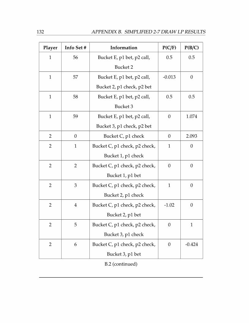
132 APPENDIX B. SIMPLIFIED 2-7 DRAW LP RESULTS
Player Info Set # Information P(C/F) P(B/C)
1 56 Bucket E, p1 bet, p2 call,
Bucket 2
0.5 0.5
1 57 Bucket E, p1 bet, p2 call,
Bucket 2, p1 check, p2 bet
-0.013 0
1 58 Bucket E, p1 bet, p2 call,
Bucket 3
0.5 0.5
1 59 Bucket E, p1 bet, p2 call,
Bucket 3, p1 check, p2 bet
0 1.074
2 0 Bucket C, p1 check 0 2.093
2 1 Bucket C, p1 check, p2 check,
Bucket 1, p1 check
1 0
2 2 Bucket C, p1 check, p2 check,
Bucket 1, p1 bet
0 0
2 3 Bucket C, p1 check, p2 check,
Bucket 2, p1 check
1 0
2 4 Bucket C, p1 check, p2 check,
Bucket 2, p1 bet
-1.02 0
2 5 Bucket C, p1 check, p2 check,
Bucket 3, p1 check
0 1
2 6 Bucket C, p1 check, p2 check,
Bucket 3, p1 bet
0 -0.424
B.2 (continued)
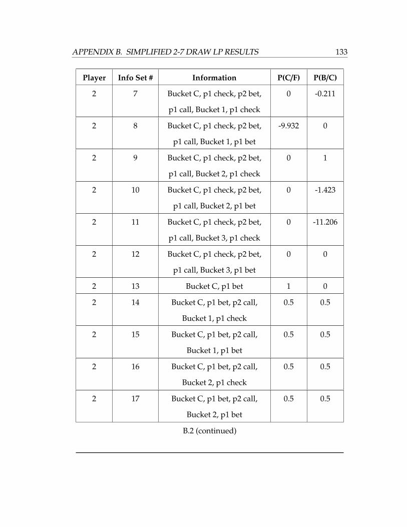
APPENDIX B. SIMPLIFIED 2-7 DRAW LP RESULTS 133
Player Info Set # Information P(C/F) P(B/C)
2 7 Bucket C, p1 check, p2 bet,
p1 call, Bucket 1, p1 check
0 -0.211
2 8 Bucket C, p1 check, p2 bet,
p1 call, Bucket 1, p1 bet
-9.932 0
2 9 Bucket C, p1 check, p2 bet,
p1 call, Bucket 2, p1 check
0 1
2 10 Bucket C, p1 check, p2 bet,
p1 call, Bucket 2, p1 bet
0 -1.423
2 11 Bucket C, p1 check, p2 bet,
p1 call, Bucket 3, p1 check
0 -11.206
2 12 Bucket C, p1 check, p2 bet,
p1 call, Bucket 3, p1 bet
0 0
2 13 Bucket C, p1 bet 1 0
2 14 Bucket C, p1 bet, p2 call,
Bucket 1, p1 check
0.5 0.5
2 15 Bucket C, p1 bet, p2 call,
Bucket 1, p1 bet
0.5 0.5
2 16 Bucket C, p1 bet, p2 call,
Bucket 2, p1 check
0.5 0.5
2 17 Bucket C, p1 bet, p2 call,
Bucket 2, p1 bet
0.5 0.5
B.2 (continued)
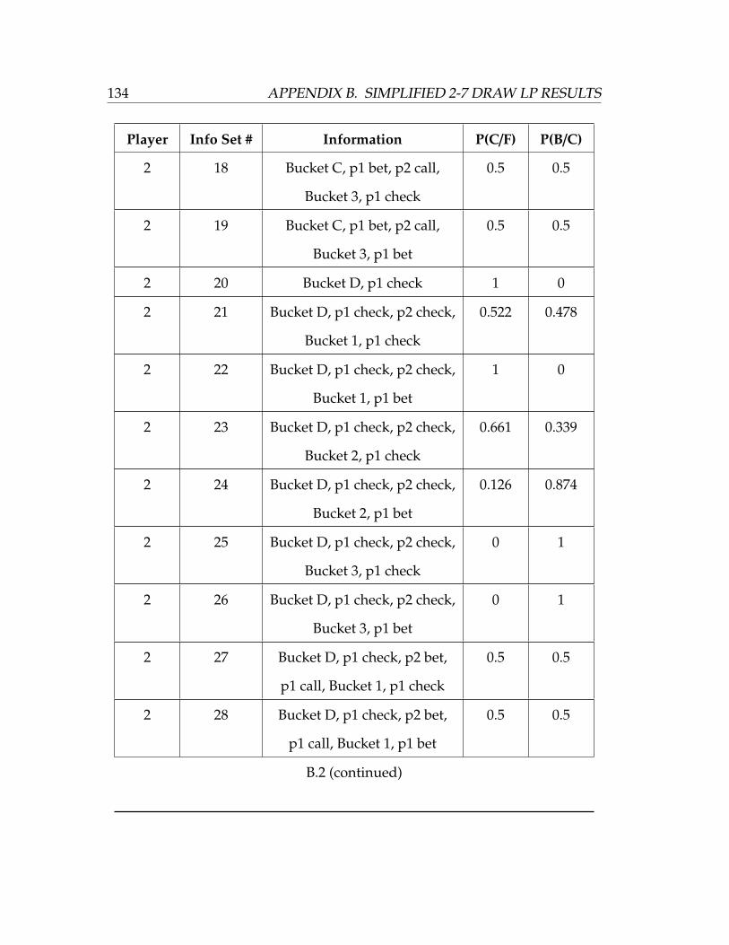
134 APPENDIX B. SIMPLIFIED 2-7 DRAW LP RESULTS
Player Info Set # Information P(C/F) P(B/C)
2 18 Bucket C, p1 bet, p2 call,
Bucket 3, p1 check
0.5 0.5
2 19 Bucket C, p1 bet, p2 call,
Bucket 3, p1 bet
0.5 0.5
2 20 Bucket D, p1 check 1 0
2 21 Bucket D, p1 check, p2 check,
Bucket 1, p1 check
0.522 0.478
2 22 Bucket D, p1 check, p2 check,
Bucket 1, p1 bet
1 0
2 23 Bucket D, p1 check, p2 check,
Bucket 2, p1 check
0.661 0.339
2 24 Bucket D, p1 check, p2 check,
Bucket 2, p1 bet
0.126 0.874
2 25 Bucket D, p1 check, p2 check,
Bucket 3, p1 check
0 1
2 26 Bucket D, p1 check, p2 check,
Bucket 3, p1 bet
0 1
2 27 Bucket D, p1 check, p2 bet,
p1 call, Bucket 1, p1 check
0.5 0.5
2 28 Bucket D, p1 check, p2 bet,
p1 call, Bucket 1, p1 bet
0.5 0.5
B.2 (continued)
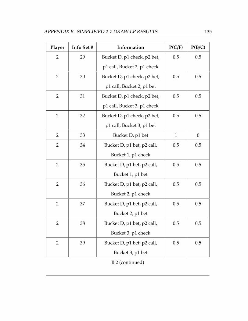
APPENDIX B. SIMPLIFIED 2-7 DRAW LP RESULTS 135
Player Info Set # Information P(C/F) P(B/C)
2 29 Bucket D, p1 check, p2 bet,
p1 call, Bucket 2, p1 check
0.5 0.5
2 30 Bucket D, p1 check, p2 bet,
p1 call, Bucket 2, p1 bet
0.5 0.5
2 31 Bucket D, p1 check, p2 bet,
p1 call, Bucket 3, p1 check
0.5 0.5
2 32 Bucket D, p1 check, p2 bet,
p1 call, Bucket 3, p1 bet
0.5 0.5
2 33 Bucket D, p1 bet 1 0
2 34 Bucket D, p1 bet, p2 call,
Bucket 1, p1 check
0.5 0.5
2 35 Bucket D, p1 bet, p2 call,
Bucket 1, p1 bet
0.5 0.5
2 36 Bucket D, p1 bet, p2 call,
Bucket 2, p1 check
0.5 0.5
2 37 Bucket D, p1 bet, p2 call,
Bucket 2, p1 bet
0.5 0.5
2 38 Bucket D, p1 bet, p2 call,
Bucket 3, p1 check
0.5 0.5
2 39 Bucket D, p1 bet, p2 call,
Bucket 3, p1 bet
0.5 0.5
B.2 (continued)
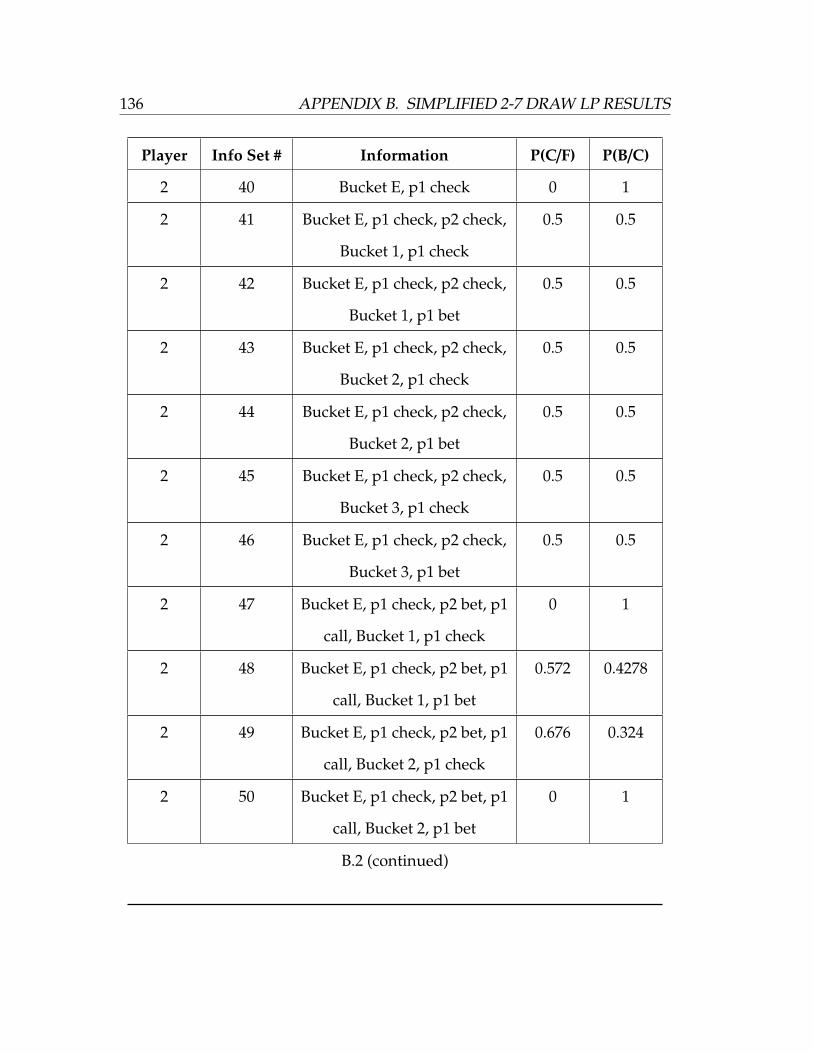
136 APPENDIX B. SIMPLIFIED 2-7 DRAW LP RESULTS
Player Info Set # Information P(C/F) P(B/C)
2 40 Bucket E, p1 check 0 1
2 41 Bucket E, p1 check, p2 check,
Bucket 1, p1 check
0.5 0.5
2 42 Bucket E, p1 check, p2 check,
Bucket 1, p1 bet
0.5 0.5
2 43 Bucket E, p1 check, p2 check,
Bucket 2, p1 check
0.5 0.5
2 44 Bucket E, p1 check, p2 check,
Bucket 2, p1 bet
0.5 0.5
2 45 Bucket E, p1 check, p2 check,
Bucket 3, p1 check
0.5 0.5
2 46 Bucket E, p1 check, p2 check,
Bucket 3, p1 bet
0.5 0.5
2 47 Bucket E, p1 check, p2 bet, p1
call, Bucket 1, p1 check
0 1
2 48 Bucket E, p1 check, p2 bet, p1
call, Bucket 1, p1 bet
0.572 0.4278
2 49 Bucket E, p1 check, p2 bet, p1
call, Bucket 2, p1 check
0.676 0.324
2 50 Bucket E, p1 check, p2 bet, p1
call, Bucket 2, p1 bet
0 1
B.2 (continued)
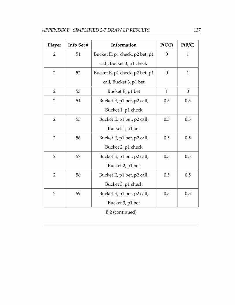
APPENDIX B. SIMPLIFIED 2-7 DRAW LP RESULTS 137
Player Info Set # Information P(C/F) P(B/C)
2 51 Bucket E, p1 check, p2 bet, p1
call, Bucket 3, p1 check
0 1
2 52 Bucket E, p1 check, p2 bet, p1
call, Bucket 3, p1 bet
0 1
2 53 Bucket E, p1 bet 1 0
2 54 Bucket E, p1 bet, p2 call,
Bucket 1, p1 check
0.5 0.5
2 55 Bucket E, p1 bet, p2 call,
Bucket 1, p1 bet
0.5 0.5
2 56 Bucket E, p1 bet, p2 call,
Bucket 2, p1 check
0.5 0.5
2 57 Bucket E, p1 bet, p2 call,
Bucket 2, p1 bet
0.5 0.5
2 58 Bucket E, p1 bet, p2 call,
Bucket 3, p1 check
0.5 0.5
2 59 Bucket E, p1 bet, p2 call,
Bucket 3, p1 bet
0.5 0.5
B.2 (continued)
138 APPENDIX B. SIMPLIFIED 2-7 DRAW LP RESULTS

Bibliography
[1] Rickard Andersson. Pseudo-Optimal Strategies in No-Limit Poker.
Master’s thesis, Umea University, 2006.
[2] D. Billings, N. Burch, A. Davidson, R. Holte, J. Schaeffer, T. Schauenberg,
and D. Szafron. Approximating Game-Theoretic Optimal Strategies for
Full-Scale Poker. Proceedings of the 18th International Joint Conference on
Artificial Intelligence, 2003. University of Alberta.
[3] Michael Bowling, Neil Burch, Michael Johanson, and Oskari Tammelin.
Heads-up Limit Holdem Poker is Solved. Science, 347(6218):145–149, 2015.
[4] Drew Fudenberg and Jean Tirole. Game Theory. Massachusetts Institute of
Technology, Boston, MA, 1995.
[5] Harold W. Kuhn. Contributions to the Theory of Games, pages 97–103.
Princeton University Press, 1950.
[6] Richard D. McKelvey, Andrew M. McLennan, and Theodore L. Turocy.
139
140 BIBLIOGRAPHY
Gambit: Software Tools for Game Theory, Version 15.1.0, 2014.
http://www.gambit-project.org.
[7] Martin J. Osborne and Ariel Rubinstein. A Course in Game Theory.
Massachusetts Institute of Technology Press, 1994.
[8] Pokerstars. 2-7 (Deuce to Seven) Single Draw Lowball Rules, 2017.
https://www.pokerstars.com/poker/games/draw/2-7/single/.
[9] Tuomas Sandholm and Andrew Gilpin. Optimal Rhode Island Hold’em
Poker. National Conference on Artificial Intelligence (AAAI), Intelligent
Systems Demonstration Program, 2005.
[10] Byron Spice. Carnegie Mellon Artificial Intelligence Beats Top Poker
Pros. 2017. https://www.cmu.edu/news/stories/archives/2017/january/AI-
beats-poker-pros.html.
[11] Ted Turocy. Personal correspondence. Gambit Technical Support, 2017.
https://github.com/gambitproject/gambit/issues/211.
[12] Robert J. Vanderbei. Linear Programming: Foundations and Extensions.
Springer US, Boston, MA, 2014.
[13] Bernhard von Stengel. Efficient Computation of Behavior Strategies.
Games and Economic Behavior, 14:220–246, 1996.