Embed Size (px)
Citation preview
DRAFT VERSION APRIL 27, 2018Typeset using LATEX twocolumn style in AASTeX61
THE SECOND APOKASC CATALOG: THE EMPIRICAL APPROACH
MARC H. PINSONNEAULT,1 YVONNE P. ELSWORTH,2, 3 JAMIE TAYAR,1 ALDO SERENELLI,4 DENNIS STELLO,5 JOEL ZINN,1
SAVITA MATHUR,6, 7, 8 RAFAEL A. GARCÍA,9, 10 JENNIFER A. JOHNSON,1, 11 SASKIA HEKKER,12, 3 DANIEL HUBER,13
THOMAS KALLINGER,14 SZABOLCS MÉSZÁROS,15, 16 BENOIT MOSSER,17 KEIVAN STASSUN,18 LÉO GIRARDI,19
THAÍSE S. RODRIGUES,19 VICTOR SILVA AGUIRRE,3 DEOKKEUN AN,20 SARBANI BASU,21 WILLIAM J. CHAPLIN,2, 3
ENRICO CORSARO,22 KATIA CUNHA,23, 24 D. A. GARCÍA-HERNÁNDEZ,6, 7 JON HOLTZMAN,25 HENRIK JÖNSSON,26
MATTHEW SHETRONE,27 VERNE V. SMITH,28 JENNIFER S. SOBECK,29 GUY S. STRINGFELLOW,30 OLGA ZAMORA,6, 7
TIMOTHY C. BEERS,31 J. G. FERNÁNDEZ-TRINCADO,32, 33 PETER M. FRINCHABOY,34 FRED R. HEARTY,35 AND
CHRISTIAN NITSCHELM36
1Department of Astronomy, The Ohio State University, Columbus, OH 43210, USA2University of Birmingham, School of Physics and Astronomy, Edgbaston, Birmingham B15 2TT, UK3Stellar Astrophysics Centre, Department of Physics and Astronomy, Aarhus University, Ny Munkegade 120, DK-8000 Aarhus C, Denmark4Institute of Space Sciences (IEEC-CSIC), Campus UAB, E-08193 Bellaterra, Spain5School of Physics, University of New South Wales, NSW 2052, Australia6Instituto de Astrofsica de Canarias (IAC), C/Va Lactea, s/n, E-38200 La Laguna, Tenerife, Spain7Universidad de La Laguna (ULL), Departamento de Astrofísica, E-38206 La Laguna, Tenerife, Spain8Space Science Institute, 4750 Walnut street, Suite 205, Boulder, CO 80301, USA9Université Paris Diderot, AIM, Sorbonne Paris Cité, CEA, CNRS, F-91191 Gif-sur-Yvette, France10IRFU, CEA, Université Paris-Saclay, F-91191 Gif-sur-Yvette, France11Center for Cosmology and Astroparticle Physics, The Ohio State University, Columbus, OH 43210, USA12Max-Planck-Institut für Sonnensystemforschung, Justus-von-Liebig-Weg 3, D-37077 Gottingen, Germany13Institute for Astronomy, University of Hawaii, 2680 Woodlawn Drive, Honolulu, HI 96822, USA14Institute for Astronomy, University of Vienna, Türkenschanzstrasse 17, A-1180 Vienna, Austria15ELTE Eötvös Loránd University, Gothard Astrophysical Observatory, Szombathely, Hungary16Premium Postdoctoral Fellow of the Hungarian Academy of Sciences17LESIA, Observatoire de Paris, PSL Research University, CNRS, Université Pierre et Marie Curie, Université Paris Diderot, 92195 Meudon, France18Department of Physics and Astronomy, Vanderbilt University, Nashville, TN 37235, USA19Osservatorio Astronomico di Padova, INAF, Vicolo dell Osservatorio 5, I35122 Padova, Italy20Department of Science Education, Ewha Womans University, 52 Ewhayeodae-gil, Seodaemun-gu, Seoul 03760, Korea21Department of Astronomy, Yale University, PO Box 208101, New Haven CT, 06520-810122INAF - Osservatorio Astrofisico di Catania, via S. Sofia 78, 95123 Catania, Italy23University of Arizona, Tucson, AZ 85719, USA24Observatório Nacional, São Cristóvão, Rio de Janeiro, Brazil25Department of Astronomy, MSC 4500, New Mexico State University, P.O. Box 30001, Las Cruces, NM 88003, USA26Lund Observatory, Department of Astronomy and Theoretical Physics, Lund University, Box 43, SE-22100 Lund, Sweden27University of Texas at Austin, McDonald Observatory, 32 Fowlkes Road, TX 79734-3005, USA28National Optical Astronomy Observatories, Tucson, AZ 85719 USA29Department of Astronomy Box 351580, U.W. University of Washington Seattle, WA 98195-158030Center for Astrophysics and Space Astronomy, Department of Astrophysical and Planetary Sciences, University of Colorado, 389 UCB, Boulder Colorado
80309-038931Dept. of Physics and JINA Center for the Evolution of the Elements University of Notre Dame, Notre Dame, IN 46556 USA32Departamento de Astronomí a, Casilla 160-C, Universidad de Concepción, Concepción, Chile33Institut Utinam, CNRS UMR6213, Univ. Bourgogne Franche-Comté, OSU THETA , Observatoire de Besançon, BP 1615, 25010 Besançon Cedex, France34Department of Physics & Astronomy, Texas Christian University, Fort Worth, TX 76129, USA35Department of Astronomy and Astrophysics Pennsylvania State University 525 Davey Laboratory University Park PA 16802 USA36Unidad de Astronomía, Facultad de Ciencias Básicas, Universidad de Antofagasta, Antofagasta, Chile
arX
iv:1
804.
0998
3v1
[as
tro-
ph.S
R]
26
Apr
201
8
2 PINSONNEAULT ET AL.
ABSTRACT
We present a catalog of stellar properties for a large sample of 6676 evolved stars with APOGEE spectroscopic parametersand Kepler asteroseismic data analyzed using five independent techniques. Our data includes evolutionary state, surface gravity,mean density, mass, radius, age, and the spectroscopic and asteroseismic measurements used to derive them. We employ a newempirical approach for combining asteroseismic measurements from different methods, calibrating the inferred stellar parameters,and estimating uncertainties. With high statistical significance, we find that asteroseismic parameters inferred from the differentpipelines have systematic offsets that are not removed by accounting for differences in their solar reference values. We includetheoretically motivated corrections to the large frequency spacing (∆ν) scaling relation, and we calibrate the zero point of thefrequency of maximum power (νmax) relation to be consistent with masses and radii for members of star clusters. For mosttargets, the parameters returned by different pipelines are in much better agreement than would be expected from the pipeline-predicted random errors, but 22% of them had at least one method not return a result and a much larger measurement dispersion.This supports the usage of multiple analysis techniques for asteroseismic stellar population studies. The measured dispersionin mass estimates for fundamental calibrators is consistent with our error model, which yields median random and systematicmass uncertainties for RGB stars of order 4%. Median random and systematic mass uncertainties are at the 9% and 8% levelrespectively for RC stars.
Keywords: stars:abundances — stars:fundamental parameters —stars:oscillations
APOKASC 2 3
1. INTRODUCTION
Stellar astrophysics is in the midst of a dramatic transfor-mation. We are moving from a domain defined by small,local and disjoint data sets into an era where we have richtime domain information, complemented by spectroscopic,photometric, and astrometric surveys for large populations ofstars across the Milky Way galaxy. In this paper we presentthe second release of the joint APOKASC asteroseismic andspectroscopic survey. Our targets have high-resolution H-band spectra from the Apache Point Observatory GalacticEvolution Experiment (APOGEE) project (Majewski et al.2017) which were obtained during the third Sloan Digital SkySurvey, hereafter SDSS-III (Eisenstein et al. 2011) and ana-lyzed during the fourth Sloan Digital Sky Survey, hereafterSDSS-IV (Blanton et al. 2017). Our asteroseismic data wasobtained by the Kepler mission (Borucki et al. 2010), ana-lyzed by members of the Kepler Asteroseismology ScienceConsortium (KASC), and interpreted by the team using bothasteroseismic and spectroscopic data.
The primary scientific goal of the APOGEE project is re-constructing the formation history of the Milky Way galaxythrough detailed studies of its stellar populations. This is fre-quently referred to as Galactic archeology. The relativelyhigh resolution (R∼22,000) of the spectra permits detailedstellar characterization. The infrared spectra from APOGEEcan reach targets that would be heavily obscured in the opti-cal, and the combination of a relatively large field of view (6square degrees) and multi-plexing (300 fibers per plate) canyield large samples of representative Galactic stellar popula-tions. Evolved low-mass stars (both H-shell burning, or redgiant stars, and He-core burning, or red clump stars) are theprimary targets for APOGEE because they are intrinsicallyluminous, relatively common, and their H-band spectra areinformation-rich.
Despite these attractive features, there are drawbacks as-sociated with using red giant and clump stars for popula-tion studies. Using spectra alone, it is difficult to infer ages,crucial for tracing the evolution of populations, because stel-lar evolution transforms stars with a wide range of main se-quence temperatures and luminosities into cool giants witha relatively narrow range of properties. As a consequence,indirect age proxies - for example, kinematics, or abundancemixtures associated with youth or age, have to be employedby spectroscopic surveys working alone.
The combination of spectroscopic and asteroseismic datais powerful, however, and both can now be measured forthousands of evolved cool stars. Large space-based planettransit surveys such as CoRoT and Kepler naturally producedetailed information on stellar variability with a cadence ide-ally suited to detecting oscillations in giants (de Ridder et al.2009; Bedding et al. 2010). These oscillation patterns encodedetailed information about their structure and global prop-
erties. A major application for stellar population studies isthe discovery that the frequency pattern can be used to dis-tinguish between shell H-burning (or red giant) stars, withdegenerate cores, and core He-burning (or red clump) stars,whose cores are larger and much less dense (Bedding et al.2011). For some targets, detailed studies of the measuredfrequencies can also be used to study features such as inter-nal stellar rotation (Beck et al. 2012; Deheuvels et al. 2012).However, for bulk stellar populations, there is still powerfulinformation in two key measures of the oscillation patternwhich can be measured for large samples: the frequency ofmaximum power, νmax, and the large frequency spacing ∆ν.
The well-studied solar oscillation frequency pattern servesas a benchmark, with a νmax of order 3100 µHz (five minutes)and ∆ν around 135 µHz. Because the acoustic cut-off fre-quency is related to the surface gravity (Kjeldsen & Bedding1995), we can adopt a semi-empirical scaling relation of theform
fνmax
(νmax
νmax,�
)=(
MM�
)(R
R�
)−2( Teff
Teff,�
)−0.5
(1)
In this equation the factor fνmax can be a scalar or a func-tion that captures deviations from the scaling relation. It canbe shown analytically that the square of the large frequencyspacing ∆ν is proportional to the mean density in the limitingcase of homology and large radial order n (Ulrich 1986). Wecan therefore define an analogous scaling relation for ∆ν,
f∆ν
(∆ν
∆ν�
)=(
MM�
)0.5( RR�
)−1.5
(2)
The term f∆ν can be computed from a detailed stellarmodel, and is in general a function of both the initial con-ditions and the current evolutionary state. In simple scalingrelations f∆ν = fνmax = 1, and the mass and radius (Msc andRsc) are defined by
(Msc
M�
)=(νmax
νmax,�
)3( Teff
Teff,�
)1.5(∆ν
∆ν�
)−4
(3)
and (Rsc
R�
)=(νmax
νmax,�
)(Teff
Teff,�
)0.5(∆ν
∆ν�
)−2
(4)
In Pinsonneault et al. (2014), which we will refer to asAPOKASC-1, we presented the first major catalog using bothasteroseismic and spectroscopic data for a large sample of redgiants. There are two natural applications of this approach:detailed studies of stellar physics and studies of stellar popu-lations. The availability of simultaneous mass and compo-sition data can be used to search for correlations between
4 PINSONNEAULT ET AL.
mass, age and spectroscopic observables. This is an espe-cially exciting prospect because the set of stars with spec-troscopic data from large surveys greatly exceeds the samplewith asteroseismic data, which can be used to calibrate suchrelationships. For example, the surface [C/N] abundance is aproduct of the first dredge-up on the red giant branch, whichis both expected on theoretical grounds to be mass and com-position dependent (Salaris et al. 2015) and observed to beso in open cluster data (Tautvaisiene et al. 2015). Data setsprior to APOGEE, however, were sparse and the sampleswere small. APOKASC-1 data was used to calibrate massusing both [C/N] (Martig et al. 2016) and the full APOGEEspectra (Ness et al. 2016) using the CANNON methodology.This approach has also been used for stellar population stud-ies (Silva Aguirre et al. 2017).
Another early result from the APOKASC-1 data was thediscovery of a significant population of high-mass stars withhigh [α/Fe] by Martig et al. (2015); this was discovered inde-pendently by Chiappini et al. (2015) using a combination ofCoRoT and APOGEE data in the related CoRoGEE project.This is a striking result because high-[α/Fe] stars are typi-cally regarded as a purely old, and by extension low-mass,population. Some of these objects are evolved blue strag-glers, or merger products (Jofre et al. 2017), but explain-ing all of them with this channel would require a very highmerger rate (Izzard et al. 2018). The alternative is an un-usual nucleosynthetic origin; see Chiappini et al. (2015) fora discussion. The discovery and characterization of unusualchemical stellar populations is a major prospect for Galacticarcheology in general, as is the understanding of the prod-ucts of binary star interactions. The joint data set has alsoenabled detailed studies of stellar physics, including tests ofmodels of extra-mixing on the red giant branch (Masseron etal. 2017) and of the structure of core-He burning stars (Con-stantino et al. 2015; Bossini et al. 2017).
However, there are recognized drawbacks to the approachused in the initial paper. Important populations, such asmembers of open clusters, very metal-poor stars, and lumi-nous giants were relatively sparsely sampled. Of more im-port, the APOKASC-1 effort did not attempt to calibrate themasses, radii, and uncertainties against fundamental data.This is not a priori unreasonable, as initial checks of aster-oseismic radii against interferometric values (Huber et al.2012) and those inferred from Hipparcos parallaxes com-bined with Teff (Silva Aguirre et al. 2012) found encourag-ing agreement at the 5% level. However, even early on therewas a recognized tension between masses derived from sim-ple scaling relations and those expected for red giants in theold open cluster NGC 6791 (Brogaard et al. 2012). Withthe advent of the APOKASC-1 catalog, larger field star sam-ples could be obtained and additional tests were possible.The masses for halo stars derived from scaling relations in
APOKASC-1 were found to be well above astrophysicallyreasonable values for old stellar populations (Epstein et al.2014). Offsets between fundamental and asteroseismic massand radius values were also found for eclipsing binary stars(Gaulme et al. 2016). These results highlighted the need forimprovements in the overall approach, which we now de-scribe.
1.1. Differences with Prior Work and the Grid ModelingEffort.
The APOKASC-1 catalog contained asteroseismic andspectroscopic data for 1916 stars. Since that time there hasbeen both a substantial increase in the sample size and achange in the data analysis techniques. The APOKASC-1approach used spectroscopic data from the tenth data release(hereafter DR10) of the Sloan Digital Sky Survey (Ahn etal. 2010); two different temperature scales were consideredto account for scale shifts in spectroscopic data. The as-teroseismic analysis was based on standard scaling relations.Measurements and theoretically estimated random uncertain-ties were taken from a single analysis pipeline with averageresults close to the mean of the measurements from all meth-ods. Differences between pipelines were then used to infersystematic uncertainties and added in quadrature to the ran-dom ones to derive a total error budget. Our final stellarproperties were derived including constraints from both theasteroseismic parameters and stellar interior models (a pro-cedure usually called grid-based modeling). In our revisedcatalog we critically examine each of these assumptions.
The spectroscopic pipeline has been extensively tested andmodified since DR10 (see Section 2.2 below); the key in-gredient for our purposes is Teff, which enters directly intothe formulas for asteroseismic surface gravities, masses andradii. If grid modeling is being performed, Teff, [Fe/H] and[α/Fe] are needed to predict stellar parameters from evolu-tionary tracks. The effective temperature is a defined quan-tity that can be measured in stars with known radius and totalluminosity; such stars define a true fundamental Teff refer-ence system. Because the revised APOGEE effective tem-peratures are tied to the IRFM fundamental scale (Holtzmanet al. 2015), we do not explicitly consider different overalltemperature scales in the current effort. We have, however,assessed the impact of systematic changes in the underly-ing methodology by comparing results from the same starsfor different SDSS data releases; the differences in derivedmasses arising from adopting DR13 as opposed to DR14 pa-rameters are less than 1% in mass with small scatter, whichis well below other identified error sources.
We employ multiple methods for measuring the asteroseis-mic parameters νmax and ∆ν. In APOKASC-1 we adoptedwhat the solar-scaled hypothesis, assuming that the measure-ments themselves are all scaled relative to a method-specific
APOKASC 2 5
solar reference value. So, if a given analysis method returnsa solar νmax 10% lower than the norm, all of the νmax mea-surements would be expected to be systematically 10% lowerthan other techniques. In this paper we replace the solar-scaled hypothesis with a data-driven approach for comparingthe measurements; we have also revised our techniques forestimating both random and systematic measurement uncer-tainties.
Once we have a set of asteroseismic and spectroscopic ob-servables, we then convert them to inferred masses and radiivia scaling relations. The ∆ν scaling relation is theoreti-cally well-motivated but not expected to be exact (Stello etal. 2009; White et al. 2011). In a detailed study, Belkacemet al. (2013) studied the physics of the asteroseismic scalingrelation for ∆ν, emphasizing how departures from homol-ogy in the structures of evolved stars perturb the scaling re-lation. We therefore explore theoretically motivated correc-tions to the ∆ν scaling relation, which are known to improveagreement between asteroseismic stellar parameters and fun-damental ones (Sharma et al. 2016; Rodrigues et al. 2017;Handberg et al. 2017). These corrections are sensitive to theinternal structure, so knowledge of the evolutionary state isessential; evolutionary state is also important for ages. Wetherefore also include asteroseismic and spectroscopic evolu-tionary state measurements in this paper. This was not donein APOKASC-1, which did not report ages or use correc-tions.
The empirical νmax scaling relation has a weaker theoret-ical basis than the ∆ν scaling relation, although there havebeen detailed physical studies of its basis (Belkacem et al.2011). Despite this concern, it performs well when comparedwith empirical data. However, adjustments in the zero pointfor evolved stars are certainly reasonable, and different meth-ods also yield different values even for the Sun. We thereforetreat the absolute zero point for the νmax scaling relation as afree parameter which can be calibrated against fundamentalmass data.
Finally, we consider the impact of adopting grid-basedmodeling for evolved red giant stars. Grid-based modelingis in principle powerful, because it includes all of the con-straints from observables and theory on the derived proper-ties of the star. For stars on or near the main sequence, pre-cisely measured Teff, log g and abundances can set stringentconstraints on mass and radius that complement asteroseis-mic measurements; see Serenelli et al. (2017) for our discus-sion in the dwarf context. Unfortunately, one cannot test thevalidity of the underlying models if their accuracy is assumedin the solution, and Tayar et al. (2017) found significant off-sets between theoretical expectations from solar-calibratedisochrones and APOKASC data. The origin of these differ-ences may be in the treatment of the mixing length, as notedin that paper and by Li et al. (2018), or it may be tied to other
choices of input physics as discussed Salarais et al. (2018). Ineither case, there is no guarantee that solar calibrated modelsagree in the mean with data for evolved stars. A direct conse-quence is that there will be systematic offsets between stellarproperties inferred from the tracks alone and stellar proper-ties inferred from asteroseismology alone, which can injectcomplex systematic differences in the derived stellar prop-erties unless the models are explicitly calibrated to removesuch differences. As a result, there is benefit in choosing totest the asteroseismic scale itself directly against fundamen-tal data, rather than doing so with a hybrid grid-modelingvalue. In this paper we therefore do not imposed grid-basedmodeling constraints on our observables. A companion paper(Serenelli et al. 2018) investigates asteroseismic parametersfrom our data including grid-based modeling. Finally, for us-age in stellar population studies, we have taken our data andused it to infer ages and extinctions.
In summary, the improvements and changes in ourAPOKASC-2 analysis are:
1. Our spectroscopic parameters and uncertainties aretaken from the fourteenth data release (hereafterDR14) of the Sloan Digital Sky Survey (Abolfathiet al. 2017) instead of DR10.
2. We have inferred evolutionary states for virtually allof the stars in our sample for APOKASC-2, eitherfrom asteroseismology or from spectroscopic diagnos-tics calibrated on asteroseismic observables.
3. The relative zero points for νmax and ∆ν from differentpipelines are inferred from the data, and not assumedto be strictly defined by their relative solar referencevalues.
4. With zero point differences accounted for, the scatterof the individual pipeline values about the ensemblemean is used to infer the random uncertainty for eachstar, rather than relying on formal theoretical error es-timates.
5. ∆ν- and νmax- dependent differences between individ-ual pipeline values and the ensemble mean are treatedas systematic error sources.
6. The ∆ν scaling relation is corrected with the same the-oretically motivated approach as that in Serenelli et al.(2018), rather than being treated as exact.
7. The absolute zero point of the νmax scaling relation isset by requiring agreement with fundamental radii andmasses in star clusters with asteroseismic data, as op-posed to adopting a solar reference value.
8. We do not use grid-based modeling in APOKASC-2.
6 PINSONNEAULT ET AL.
9. We provide ages and extinction estimates.
The outcome of this exercise is tabulated for the full jointsample, and the sample properties are then discussed. Theremainder of the paper is organized as follows. We discussthe sample selection in Section 2 and present our basic datathere. The relative mean asteroseismic parameters and theabsolute calibration from open cluster members are derivedin Section 3. The catalog itself is presented in Section 4 andthe conclusions are given in Section 5.
2. SAMPLE PROPERTIES: SELECTION, UNUSUALSTARS AND EVOLUTIONARY STATE
Our basic data is drawn from two sources: time domaindata derived from the Kepler satellite during the first fouryears of operation and spectroscopic data from the APOGEEsurvey of the Sloan Digital Sky Survey. In addition, we em-ployed additional photometric data for the calibrating starclusters NGC 6791 and NGC 6819 to test the absolute radiusscale. The photometric data and adopted cluster parametersare discussed in Section 3.4.
2.1. Kepler Data
The details of the Kepler data itself and the light curvereduction procedures used are described in Elsworth et al.(2018). We employed five distinct pipelines for asteroseis-mic analysis of the reduced light curves known in the liter-ature by three-letter acronyms: A2Z, CAN, COR, OCT, andSYD. We briefly reference each method below. For a moredetailed discussion of the different approaches see Serenelliet al. (2018). The same data preparation method is not usedin all cases. Two different methods were used with A2Zpreparing their own datasets following Garcia et al. (2011)and CAN, COR, OCT and SYD all using data prepared us-ing the Handberg & Lund (2014) method. A comparison andreview of the methods is given in Hekker et al. (2011) andfurther discussed in Hekker et al. (2012), where they lookedat the impact of data duration on the detectability of the oscil-lations and the precision of the parameters. For this paper, theprecise method used to determine the average asteroseismicparameters is not of major importance because here we seekto show how the differences can be mitigated. Nevertheless,we give basic references to the method of operation of eachpipeline. The A2Z pipeline was first described in Mathur etal. (2010) and, together with their method of data prepara-tion is updated in Garcia et al. (2014). The CAN pipeline isdescribed in Kallinger et al. (2010); the COR pipeline is de-scribed in Mosser & Appourchaux (2009); the OCT pipelineis described in Hekker et al. (2010); and the SYD pipeline isdescribed in Huber et al. (2009).
2.2. Spectroscopic Data
We collected the spectroscopic data using the 2.5-meterSloan Foundation telescope (Gunn et al. 2006) and theAPOGEE near-infrared spectrograph at Apache Point Ob-servatory. These spectra were obtained during SDSS-III, andthe target selection criteria for stars in the Kepler field are de-scribed in Zasowski et al. (2013). All spectra are re-reducedand re-analyzed for each data release. The procedures usedto flat-field, co-add, extract, and calibrate the spectra are de-scribed in Nidever et al. (2015). The spectra were then pro-cessed through the APOGEE Stellar Parameters and Chem-ical Abundances Pipeline, or ASPCAP (Garcia-Pérez et al.2016), which derives Teff, log g, metallicity and other prop-erties through a χ2 minimization of differences with a gridof theoretical spectra as described below.
The APOGEE survey has presented data in four SDSS datareleases. The first set of results, in Sloan DR10, was de-scribed in Meszaros et al. (2013). The subsequent DR12data analysis technique was documented in Holtzman et al.(2015), while the data released in DR13 (as well as the sub-sequent DR14) is discussed in Holtzman et al. (2018) andJönsson et al. (2018). Each data release contained both ’raw’and ’calibrated’ atmospheric parameters. The ’raw’ valuesreflect the output of the automated pipeline analysis, whilethe ’calibrated’ values can include corrections to bring theresults into agreement with external standards.
As the survey has progressed, the corrections inferred fromthe calibration process have in general become smaller, be-cause improvements implemented in ASPCAP allowed theAPOGEE team to produce more accurate and precise atmo-spheric parameters. The first APOKASC catalog was com-piled using DR10 parameters, while results presented in thispaper use DR14 parameters, the latest SDSS-IV release. Inthis section, we detail the most important improvements toASPCAP and changes in the calibration of effective temper-ature, [Fe/H] and [α/Fe] between DR10 and DR14; these in-gredients are the ones relevant to the data presented in thispaper. There have been important changes made in the reduc-tion techniques, the line list, model atmospheres and spec-trum synthesis.
Data reduction in DR13 and DR14 included improved linespread function (LSF) characterization, telluric and persis-tence correction. ASPCAP pipeline results are benchmarkedagainst the solar spectrum and that of Arcturus, with less se-cure line strengths empirically adjusted to match specifiedvalues, using the line list from Shetrone et al. (2015). A newset of Arcturus abundances has also been adopted for tuningthe line strengths. The solar reference abundances table waschanged from Grevesse & Sauval (1998) (DR10) to Asplundet al. (2005) in DR12 and onwards. Abundances of nearly23 elements are determined in DR13 and DR14, instead of 3broad indices being reported, as was the case in DR10.
APOKASC 2 7
New ATLAS model atmospheres (Meszaros et al. 2012)were computed for DR12 and are still in use in DR14 usingthe solar reference from Asplund et al. (2005). A new setof synthetic spectra were included covering the range 2500< Teff < 4000 K, based on custom MARCS atmospheres.All synthetic spectra were calculated using Turbospectrum(Alvarez & Plez 1998); previous syntheses were done usingASSeT in DR10. From DR12 onwards, a finer grid spac-ing was adopted in metallicity ([M/H]), with 0.25 dex stepsinstead of the 0.5 dex spacing used in DR10. The grid ofmodel atmospheres was also extended to a higher metallic-ity of [M/H]=+0.75. A macroturbulent velocity relation wasdetermined based on a fit with a subset of data and a macro-turbulence dimension, rather than using a fixed value.
DR13 and DR14 use a multi-step analysis through mul-tiple grids to determine the main atmospheric parameters.Initial characterization was carried out using F, GK, and Mcoarse grids. Once stars have passed quality control steps,the ASPCAP pipeline is then used to do a full solution in6D or 7D space depending on the location of the star in theHR diagram. This high dimensionality is required becausethe APOGEE spectral region is heavily influenced by CNOmolecular features. Therefore, in addition to the 4D ingre-dients typically considered in model atmosphere fits (Teff,surface gravity, overall metallicity, and microturbulence),ASPCAP also includes three additional dimensions: alpha-element enhancement (including O), C and N. The final stepis the derivation of individual abundances, which were not in-cluded in DR10, and which use spectral windows rather thanadditional dimensions in the atmospheres grid.
For DR10, effective temperatures were calibrated to bein agreement with color temperatures for stars belonging toopen and globular clusters. This comparison sample was im-proved in subsequent data releases by replacing the limitedcluster calibration set with field stars that have low extinc-tion, which have the advantage of providing many more cali-brators in a larger metallicity and surface gravity phase space.In DR10, the effective temperature correction was fairly large(around 110-200 K, depending on Teff and metallicity). AsASPCAP improved, spectroscopic temperatures showed abetter agreement with photometric ones. This resulted in nocorrection applied in the DR13 data, as published. However,a modest metallicity-dependent offset was discovered post-release; a similar metallicity-dependent temperature correc-tion was therefore introduced again for DR14. The uncer-tainty was estimated from the scatter between spectroscopicand photometric temperatures for a subsample of targets.
Metallicities in DR13 and DR14 have been calibrated toremove Teff trends using members of star clusters; the un-derlying assumption is that any systematic trends in inferredabundance within a cluster sample are analysis artifacts, ascluster stars share the same true metallicity. This is a signif-
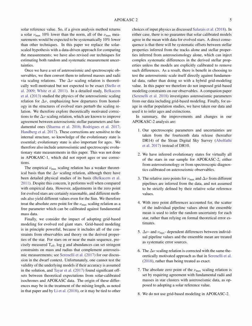
Figure 1. Spectroscopic properties in our 2014 catalog comparedwith the current values for stars in common between the two datasets. Differences are in the sense DR13-DR10 and the color reflectsthe density of points. We compare Teff in panel a, and [Fe/H] inpanel b.
icant departure from DR10, where [M/H] was calibrated tomean literature abundances for open and globular clusters asa whole, not star by star. This external calibration for [M/H]has been introduced again for DR14, but was not done inDR12 and DR13. It is important to point out that these cali-brations induce changes generally smaller than 0.1 dex, andbecome larger than that only for the most metal poor stars be-low [M/H] < -1.0. The DR14 metallicity calibration effectsare also smaller than those of DR10.
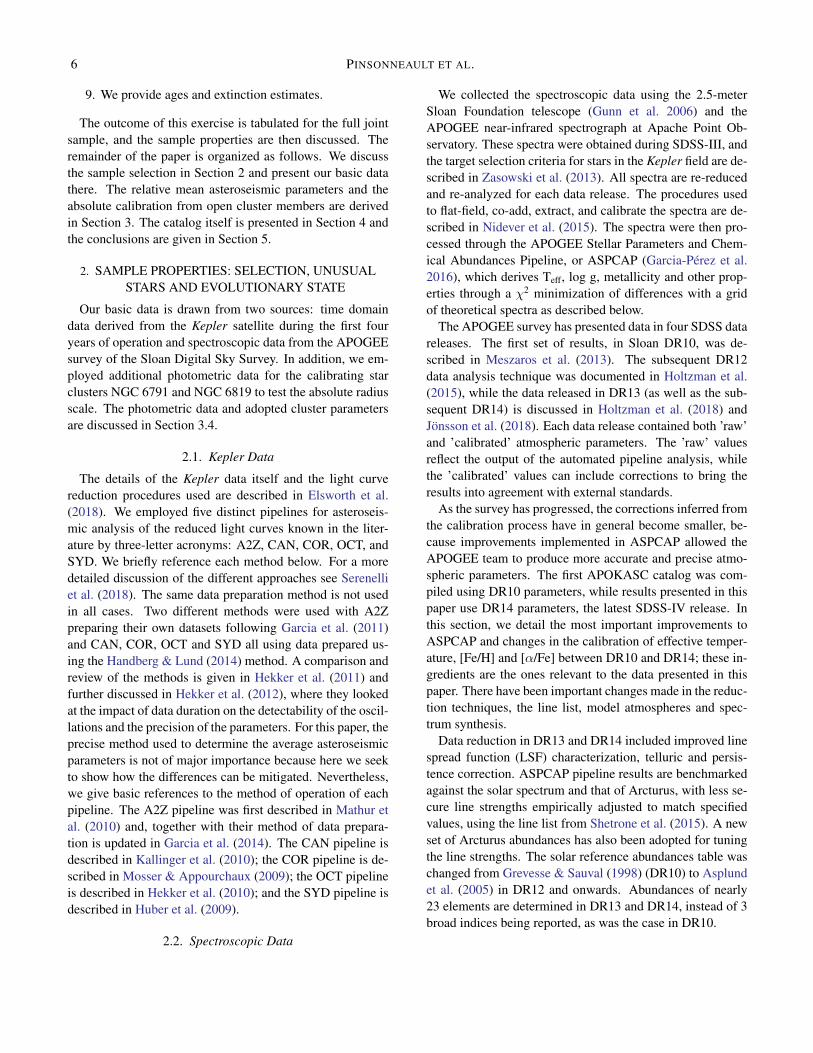
We illustrate the net impact of these changes in two fig-ures. Figure 1 compares the spectroscopic parameters forstars in APOKASC-1 between DR10 and Dr13. Systematicshifts are more important than random scatter, and the dif-ferences largely reflect changes in the choice of calibratorsfor the spectroscopic solution and improvements in the ASP-CAP spectroscopic pipeline. By comparison, the differencesbetween DR13 and DR14, illustrated in Figure 2, are milder,although there are still clear zero-point offsets in the metal-licity and scatter in the inferred carbon to nitrogen ratio, adiagnostic of the first dredge-up in evolved stars.
2.3. The SDSS-IV and APOKASC-2 Samples
The full APOGEE data sample we use was observed inSDSS-III (but analyzed in SDSS-IV) and contains 11,877stars. Many of these targets were not explicitly observed
8 PINSONNEAULT ET AL.
Figure 2. Differences in DR13 and DR14 spectroscopic propertiesin APOKASC-2 are illustrated as a function of [Fe/H]. Differencesare in the sense DR14 minus DR13 and the color reflects the densityof points. We compare Teff in panel a, [Fe/H] in panel b, and [C/N]in panel c.
for asteroseismology, however, and some of the remainderturned out to be subgiants. A total of 8604 of these stars hadcalibrated spectroscopic log g < 3.5 and were therefore po-tential red giant asteroseismic targets. Target selection forthis sample was discussed in APOKASC-1. However, notall light curves were sufficiently long to detect asteroseismicsignals; some had data artifacts; and a substantial numberin the high surface gravity domain (3.3 < log g < 3.5) aretechnically challenging to analyze because their oscillationfrequencies are close to the Kepler 30-minute sampling forlong-cadence data.
2.3.1. The Asteroseismic Parameter Calibration Sample
As discussed above, we employed 5 independent pipelinesto detect and characterize oscillations. A subset of 4706stars had data from all 5 pipelines and asteroseismic evo-lutionary states reported by Elsworth et al. (2017), and weuse this subset of the sample for our empirical calibrationof the asteroseismic measurements. As there are known dif-ferences between the asteroseismic properties of core He-burning and shell H-burning stars (Miglio et al. 2012) weanalyze them separately. In our sample of targets with resultsfrom all pipelines, 2833 objects were classified as first as-cent red giants (RGB) or as possible asymptotic giant branchstars (RGB/AGB). For the purposes of this paper we defined
any star in one of these two asteroseismically similar (Stelloet al. 2013) shell-burning categories, as RGB stars, a nota-tion that we will use for the remainder of the paper. A totalof 1873 targets are identified as either red clump (RC) stars,higher mass secondary clump (2CL) ones, or as intermediatebetween the two (RC/2CL). For the remainder of the paperwe refer to objects in this class as RC stars.
2.3.2. The Catalog Sample
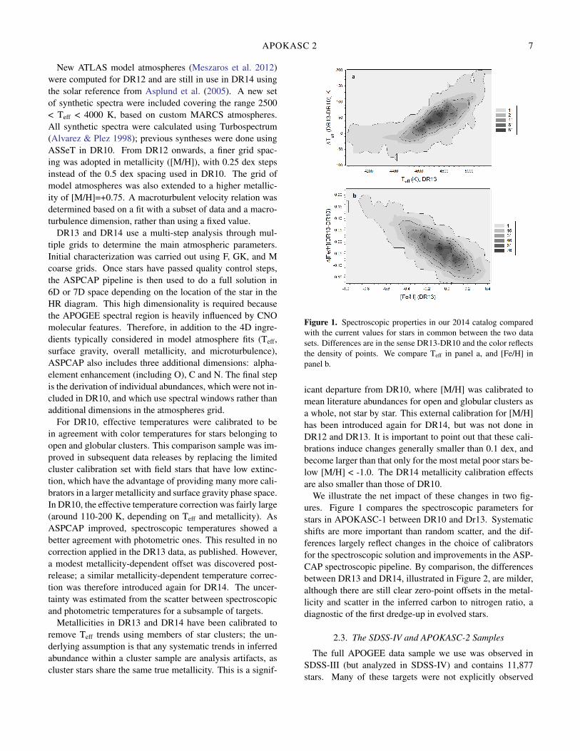
The APOKASC-2 sample analyzed in this paper contains6676 targets with reduced light curves which were selectedfor asteroseismic analysis. There are 122 stars for which wewere not able to return asteroseismic data or which had badspectra. We have asteroseismic evolutionary states for 6076of the remaining objects in Elsworth et al. (2017), including2453 RC stars and 3623 RGB stars. (The calibration set de-scribed above is smaller because we required asteroseismicparameter measurements from all pipelines for calibration,but report catalog values if any pipeline returned measure-ments.) For the 478 stars without asteroseismic evolutionarystate assignments from Elsworth et al. (2017), we infer DR13spectroscopic evolutionary states as described in Holtzman etal. (2018). This includes 276 RC stars and 152 RGB stars;only 50 stars had ambiguous evolutionary states given theirspectroscopic properties. Our data for the stars without as-teroseismic state data, and for stars with no seismic param-eters, is illustrated in Figure 3. This Kiel diagram is relatedto the classical HR Diagram, as surface gravity is related toluminosity. The cluster of targets with log g > 3.1 without re-sults are stars where the asteroseismic frequencies are closeto, or exceed, the Nyquist sampling frequency from the Ke-pler data. The remainder are an admixture of stars close tothe boundary between the RGB and the RC, where it is mostchallenging to distinguish RC from RGB stars spectroscopi-cally. This group of targets also includes a substantial num-ber of higher mass and surface gravity (log g > 2.6) core He-burning stars, and the hotter RGB sample includes a numberof very metal-poor targets. For our remaining analysis wewill treat the stars with spectroscopic evolutionary state as-signments in a manner similar to the approach taken for tar-gets with asteroseismic states; the sole exception is the groupwith ambiguous evolutionary states, for which the final massand radius estimates are more uncertain (see Section 3.2.1).A more detailed discussion of the evolutionary states of ourtargets, and a comparison of spectroscopic and asteroseismicmethods, can be found in Elsworth et al. (2018) and Holtz-man et al. (2018).
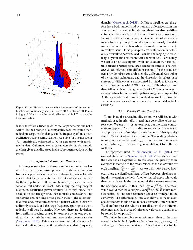
Our main sample is shown in Figure 4, and it illustratesthe power of asteroseismic evolutionary state classification.As one would expect on stellar populations grounds, the RCstars are, on average, hotter than the RGB ones. Higher massRC stars had a non-degenerate He flash, however, which pro-
APOKASC 2 9
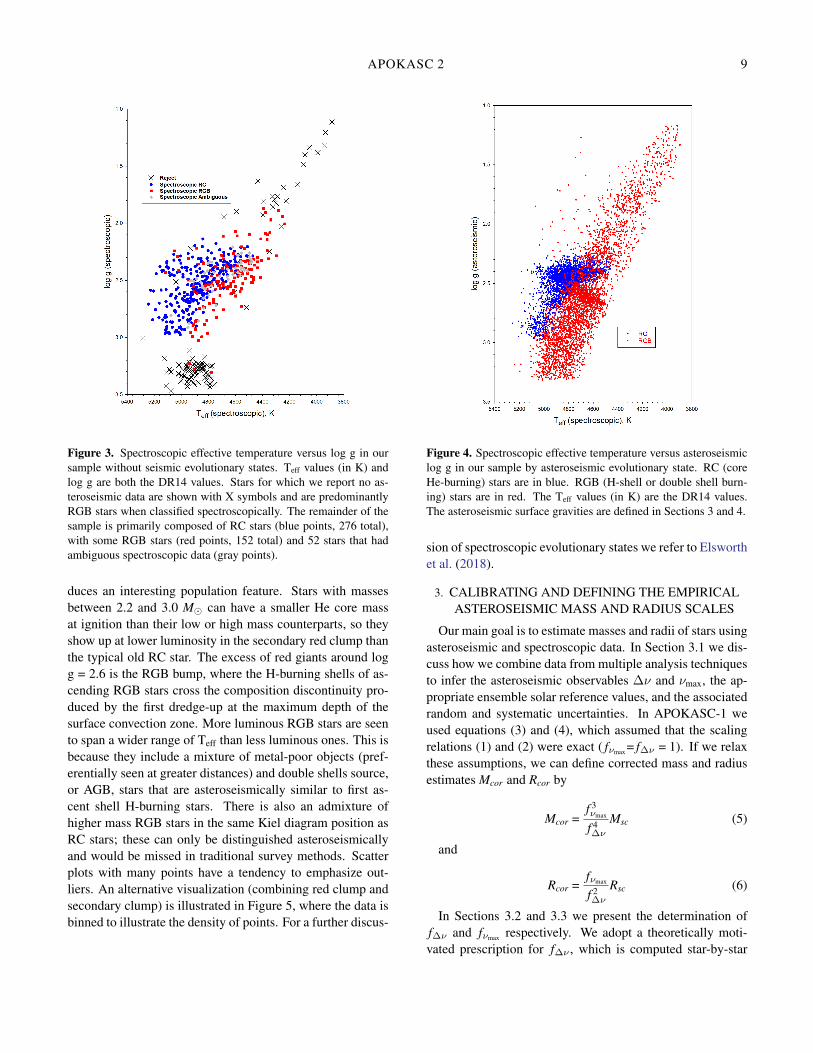
Figure 3. Spectroscopic effective temperature versus log g in oursample without seismic evolutionary states. Teff values (in K) andlog g are both the DR14 values. Stars for which we report no as-teroseismic data are shown with X symbols and are predominantlyRGB stars when classified spectroscopically. The remainder of thesample is primarily composed of RC stars (blue points, 276 total),with some RGB stars (red points, 152 total) and 52 stars that hadambiguous spectroscopic data (gray points).
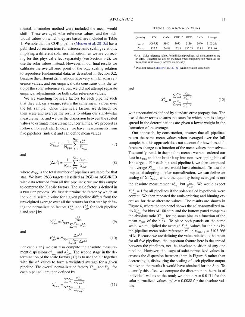
duces an interesting population feature. Stars with massesbetween 2.2 and 3.0 M� can have a smaller He core massat ignition than their low or high mass counterparts, so theyshow up at lower luminosity in the secondary red clump thanthe typical old RC star. The excess of red giants around logg = 2.6 is the RGB bump, where the H-burning shells of as-cending RGB stars cross the composition discontinuity pro-duced by the first dredge-up at the maximum depth of thesurface convection zone. More luminous RGB stars are seento span a wider range of Teff than less luminous ones. This isbecause they include a mixture of metal-poor objects (pref-erentially seen at greater distances) and double shells source,or AGB, stars that are asteroseismically similar to first as-cent shell H-burning stars. There is also an admixture ofhigher mass RGB stars in the same Kiel diagram position asRC stars; these can only be distinguished asteroseismicallyand would be missed in traditional survey methods. Scatterplots with many points have a tendency to emphasize out-liers. An alternative visualization (combining red clump andsecondary clump) is illustrated in Figure 5, where the data isbinned to illustrate the density of points. For a further discus-
Figure 4. Spectroscopic effective temperature versus asteroseismiclog g in our sample by asteroseismic evolutionary state. RC (coreHe-burning) stars are in blue. RGB (H-shell or double shell burn-ing) stars are in red. The Teff values (in K) are the DR14 values.The asteroseismic surface gravities are defined in Sections 3 and 4.
sion of spectroscopic evolutionary states we refer to Elsworthet al. (2018).
3. CALIBRATING AND DEFINING THE EMPIRICALASTEROSEISMIC MASS AND RADIUS SCALES
Our main goal is to estimate masses and radii of stars usingasteroseismic and spectroscopic data. In Section 3.1 we dis-cuss how we combine data from multiple analysis techniquesto infer the asteroseismic observables ∆ν and νmax, the ap-propriate ensemble solar reference values, and the associatedrandom and systematic uncertainties. In APOKASC-1 weused equations (3) and (4), which assumed that the scalingrelations (1) and (2) were exact ( fνmax = f∆ν = 1). If we relaxthese assumptions, we can define corrected mass and radiusestimates Mcor and Rcor by
Mcor =f 3νmax
f 4∆ν
Msc (5)
and
Rcor =fνmax
f 2∆ν
Rsc (6)
In Sections 3.2 and 3.3 we present the determination off∆ν and fνmax respectively. We adopt a theoretically moti-vated prescription for f∆ν , which is computed star-by-star
10 PINSONNEAULT ET AL.
Figure 5. As Figure 4, but counting the number of targets as afunction of evolutionary state in bins of 50 K in Teff and 0.05 dexin log g. RGB stars are the red distribution, while RC stars are theblue distribution.
(and is therefore a function of the stellar parameters and not ascalar). In the absence of a comparably well-motivated theo-retical prescription for changes in the frequency of maximumoscillation power scaling relation, we solve for a scalar factorfνmax empirically calibrated to be in agreement with funda-mental data. Calibrated stellar parameters for the full sampleare then given and discussed in the subsequent sections of thepaper.
3.1. Empirical Asteroseismic Parameters
Inferring masses from asteroseismic scaling relations hasrested on two major assumptions: that the measurementsfrom each pipeline can be scaled relative to their solar val-ues and that the uncertainties are the internal values returnedby those pipelines. Both assumptions are, in principle, rea-sonable; but neither is exact. Measuring the frequency ofmaximum oscillation power requires us to first model andaccount for the background, then to make choices about thesmoothing and/or fitting of the power excess. The asteroseis-mic frequency spectrum contains a pattern which is close touniformly spaced, and the large frequency spacing is a theo-retically well-posed quantity. However, there are deviationsfrom uniform spacing, caused for example by the way acous-tic glitches perturb the comb structure of the pressure modes(Vrard et al. 2015). This measurement must also be normal-ized and defined in a specific method-dependent frequency
domain (Mosser et al. 2013b). Different pipelines can there-fore have both random and systematic differences from oneanother that are non-negligible, and there can also be differ-ential scale factors relative to the individual solar zero-points.In practice, this means that any relative bias in solar measure-ments from a given pipeline does not necessarily translateinto a similar relative bias when it is used for measurementsin evolved stars. First principles error estimation is notori-ously difficult to perform, and it can be challenging to disen-tangle systematic and theoretical uncertainties. Fortunately,we can test both assumptions with our data set; we have mul-tiple pipeline results for a large sample of objects. The rela-tive values inferred from different methods for the same tar-gets provide robust constraints on the differential zero pointsof the various techniques, and the dispersion in values oncesystematic differences are accounted for yields guidance onerrors. We begin with RGB stars as a calibrating set, andthen follow with an analogous study of RC stars. Our astero-seismic values for individual pipelines are given in AppendixA; the values derived from our method are used to derive thestellar observables and are given in the main catalog table(Table 5).
3.1.1. Relative Pipeline Zero Points
To motivate the averaging discussion, we will begin withmethods used in prior efforts, and then generalize to the cur-rent one. We use νmax as an example, but the same consid-erations apply to ∆ν. In this discussion, 〈quantity〉 refers toa simple average of multiple measurements of that quantityfrom different pipelines for a given star. The scaling relationsrequire both a measurement (νmax in this case) and a solar ref-erence value νref
max; both are in general different for differentmethods.
The approach used in Pinsonneault et al. (2014) forevolved stars and in Serenelli et al. (2017) for dwarfs usedthe solar-scaled hypothesis. In this case, the quantity to beaveraged is the ratio of the measurement to the solar value foreach pipeline: νstar
maxνref
max= 〈 νpipe
max
νpipemax,�〉. As we will show below, how-
ever, there are significant mean offsets between pipelines us-ing this averaging method. Another logical approach wouldthen be to decouple the averaging of the measurements andthe reference values. In this limit, νstar
maxνref
max= 〈νpipe
max〉〈νmax,�〉 . The mean
value would then be a simple average of the absolute mea-surements, and the solar reference could be averaged in thesame way. The different pipelines also show significant aver-age differences in the absolute measurements, unfortunately.We therefore treat the relative normalization of the differentpipelines, and the choice of reference values, as quantities tobe solved for empirically.
We define the ensemble solar reference values as the aver-age of the individual pipeline solar values: νmax,ref = 〈νmax,�〉and ∆νref = 〈∆ν�〉 respectively. This choice is not funda-
APOKASC 2 11
mental; if another method were included the mean wouldshift. These averaged solar reference values, and the indi-vidual values on which they are based, are included in Table1. We note that the COR pipeline (Mosser et al. 2013a) has apublished correction term for asteroseismic scaling relations,implying a different solar normalization; as we are correct-ing for this physical effect separately (see Section 3.2), weuse the solar values instead. However, in our final results wecalibrate the overall zero point of the νmax scaling relationto reproduce fundamental data, as described in Section 3.2;because the different ∆ν methods have very similar solar ref-erence values, and our empirical data constrains only the ra-tio of the solar reference values, we did not attempt separateempirical adjustments for both solar reference values.
We are searching for scale factors for each pipeline suchthat they all, on average, return the same mean values overthe full sample. Once these scale factors are defined, wethen scale and average the results to obtain our star-by-starmeasurements, and we use the dispersion between the scaledvalues to estimate measurement uncertainties. We proceed asfollows. For each star (index j), we have measurements fromfive pipelines (index i) and can define mean values
〈ν jmax〉 =
1Npipe
Npipe∑I=1
ν i, jmax
X iνmax
(7)
and
〈∆ν j〉 =1
Npipe
Npipe∑I=1
∆ν i, j
X i∆ν
(8)
where Npipe is the total number of pipelines available for thatstar. We have 2833 targets classified as RGB or AGB/RGBwith data returned from all five pipelines; we use this sampleto compute the X scale factors. The scale factor is defined ina two step process. We first determine the factor by which anindividual seismic value for a given pipeline differs from theunweighted average over all the returns for that star by defin-ing the normalization factors Y i, j
νmaxand Y i, j
∆ν for each pipelinei and star j by
Y i, jνmax
= Npipeν i, j
max∑Npipei=1 ν i, j
max(9)
and
Y i, j∆ν = Npipe
∆ν i, j∑Npipei=1 ∆ν i, j
(10)
For each star j we can also compute the absolute measure-ment dispersions σ j
νmaxand σ j
∆ν . The second stage in the de-termination of the scale factors (X i) is to use the Y i j togetherwith the σ j values to form a weighted average for a givenpipeline. The overall normalization factors X i
νmaxand X i
∆ν foreach pipeline i are then defined by
X iνmax
=
∑Nstarj=1
Y i, jνmax
(σ jνmax )2∑Nstar
j=11
(σ jνmax )2
(11)
Table 1. Solar Reference Values
Quantity A2Z CAN COR a OCT SYD Average
νmax,� 3097.33 3140 3050 3139 3090 3103.266
∆ν� 135.2 134.88 135.5 135.05 135.1 135.146
NOTE—Solar reference values for individual pipelines. All measurements arein µHz. Uncertainties are not included when computing the mean, as thezero point is ultimately inferred empirically.
a Does not include Mosser et al. (2013a) scaling relation corrections
and
X i∆ν =
∑Nstarj=1
Y i, j∆ν
(σ j∆ν )2∑Nstar
j=11
(σ j∆ν )2
(12)
with uncertainties defined by standard error propagation. Theuse of the σ j terms ensures that stars for which there is a largespread in the determinations are given a lower weight in theformation of the average.
Our approach, by construction, ensures that all pipelinesreturn the same mean values when averaged over the fullsample, but this approach does not account for how these dif-ferences change as a function of the mean values themselves.To quantify trends in the pipeline means, we rank-ordered ourdata in νmax and then broke it up into non-overlapping bins of100 targets. For each bin and pipeline i, we then computedthe average X i
νmaxthat we would have obtained. To test the
impact of adopting a solar normalization, we can define ananalog of X, X
′,iνmax
, where the quantity being averaged is not
the absolute measurement ν imax but ν i
maxν i
ax,�. We would expect
X′,iνmax
= 1 for all pipelines if the solar-scaled hypothesis werecorrect. We then repeated the rank-ordering and binning ex-ercises for these alternate values. The results are shown inFigure 4, where the top panel shows the solar-normalized ra-tio X
′,iνmax
for bins of 100 stars and the bottom panel comparesthe absolute ratio X i
νmaxfor the same bins as a function of the
mean νmax of the bins. To place both panels on the samescale, we multiplied the average X
′,iνmax
values for the bins bythe pipeline mean solar reference value νmax,� = 3103.266µHz. Because we are defining the value relative to the meanfor all five pipelines, the important feature here is the spreadbetween the pipelines, not the absolute position of any onepipeline. However, the usage of solar-normalized values in-creases the dispersion between them in Figure 6 rather thandecreasing it, disfavoring the scaling of each pipeline outputrelative to the results it would have obtained for the Sun. Toquantify this effect we compute the dispersion in the ratio ofindividual values to the total; we obtain σ = 0.0131 for thesolar-normalized values and σ = 0.0088 for the absolute val-ues.
12 PINSONNEAULT ET AL.
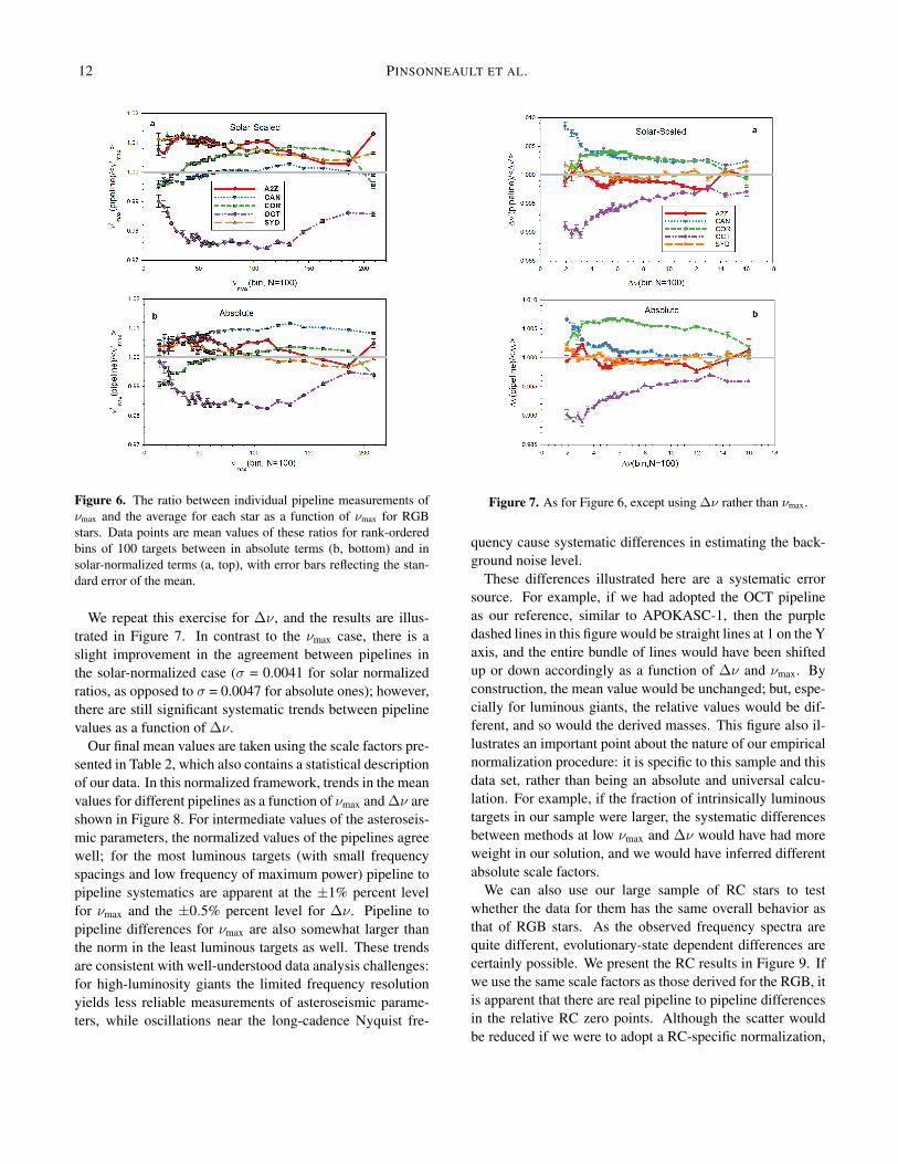
Figure 6. The ratio between individual pipeline measurements ofνmax and the average for each star as a function of νmax for RGBstars. Data points are mean values of these ratios for rank-orderedbins of 100 targets between in absolute terms (b, bottom) and insolar-normalized terms (a, top), with error bars reflecting the stan-dard error of the mean.
We repeat this exercise for ∆ν, and the results are illus-trated in Figure 7. In contrast to the νmax case, there is aslight improvement in the agreement between pipelines inthe solar-normalized case (σ = 0.0041 for solar normalizedratios, as opposed to σ = 0.0047 for absolute ones); however,there are still significant systematic trends between pipelinevalues as a function of ∆ν.
Our final mean values are taken using the scale factors pre-sented in Table 2, which also contains a statistical descriptionof our data. In this normalized framework, trends in the meanvalues for different pipelines as a function of νmax and ∆ν areshown in Figure 8. For intermediate values of the asteroseis-mic parameters, the normalized values of the pipelines agreewell; for the most luminous targets (with small frequencyspacings and low frequency of maximum power) pipeline topipeline systematics are apparent at the ±1% percent levelfor νmax and the ±0.5% percent level for ∆ν. Pipeline topipeline differences for νmax are also somewhat larger thanthe norm in the least luminous targets as well. These trendsare consistent with well-understood data analysis challenges:for high-luminosity giants the limited frequency resolutionyields less reliable measurements of asteroseismic parame-ters, while oscillations near the long-cadence Nyquist fre-
Figure 7. As for Figure 6, except using ∆ν rather than νmax.
quency cause systematic differences in estimating the back-ground noise level.
These differences illustrated here are a systematic errorsource. For example, if we had adopted the OCT pipelineas our reference, similar to APOKASC-1, then the purpledashed lines in this figure would be straight lines at 1 on the Yaxis, and the entire bundle of lines would have been shiftedup or down accordingly as a function of ∆ν and νmax. Byconstruction, the mean value would be unchanged; but, espe-cially for luminous giants, the relative values would be dif-ferent, and so would the derived masses. This figure also il-lustrates an important point about the nature of our empiricalnormalization procedure: it is specific to this sample and thisdata set, rather than being an absolute and universal calcu-lation. For example, if the fraction of intrinsically luminoustargets in our sample were larger, the systematic differencesbetween methods at low νmax and ∆ν would have had moreweight in our solution, and we would have inferred differentabsolute scale factors.
We can also use our large sample of RC stars to testwhether the data for them has the same overall behavior asthat of RGB stars. As the observed frequency spectra arequite different, evolutionary-state dependent differences arecertainly possible. We present the RC results in Figure 9. Ifwe use the same scale factors as those derived for the RGB, itis apparent that there are real pipeline to pipeline differencesin the relative RC zero points. Although the scatter wouldbe reduced if we were to adopt a RC-specific normalization,
APOKASC 2 13
Table 2. Relative Pipeline Zero Points
Quantity A2Z CAN COR OCT SYD
Xνmax ,� 0.9981 1.0118 0.9828 1.0115 0.9957
Xνmax ,RGB 1.0023(2) 1.0082(2) 0.9989(2) 0.9900(2) 1.0006(2)
Xνmax ,RC 1.0035(3) 1.0067(2) 0.9909(2) 0.9979(4) 1.0010(3)
σνmax ,RGB 0.010 0.006 0.006 0.012 0.009
X∆ν,� 1.0004 0.9980 1.0026 0.9993 0.9997
X∆ν,RGB 0.9993(1) 1.0007(1) 1.0051(1) 0.9955(1) 0.9995(1)
X∆ν,RC 0.9965(3) 1.0108(2) 0.9960(1) 0.9935(2) 1.0032(2)
σ∆ν,RGB 0.006 0.004 0.004 0.005 0.003
NOTE—Error-weighted mean ratios of values from individual pipelines to the en-semble average.
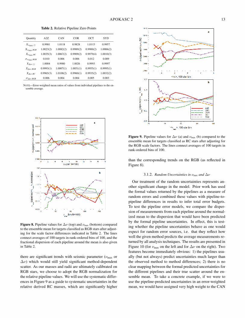
Figure 8. Pipeline values for ∆ν (top) and νmax (bottom) comparedto the ensemble mean for targets classified as RGB stars after adjust-ing for the scale factor differences indicated in Table 2. The linesconnect averages of 100 targets in rank-ordered bins of 100, and thefractional dispersion of each pipeline around the mean is also givenin Table 2.
there are significant trends with seismic parameter (νmax or∆ν) which would still yield significant method-dependentscatter. As our masses and radii are ultimately calibrated onRGB stars, we choose to adopt the RGB normalization forthe relative pipeline values. We will use the systematic differ-ences in Figure 9 as a guide to systematic uncertainties in therelative derived RC masses, which are significantly higher
Figure 9. Pipeline values for ∆ν (a) and νmax (b) compared to theensemble mean for targets classified as RC stars after adjusting forthe RGB scale factors. The lines connect averages of 100 targets inrank-ordered bins of 100.
than the corresponding trends on the RGB (as reflected inFigure 8).
3.1.2. Random Uncertainties in νmax and ∆ν
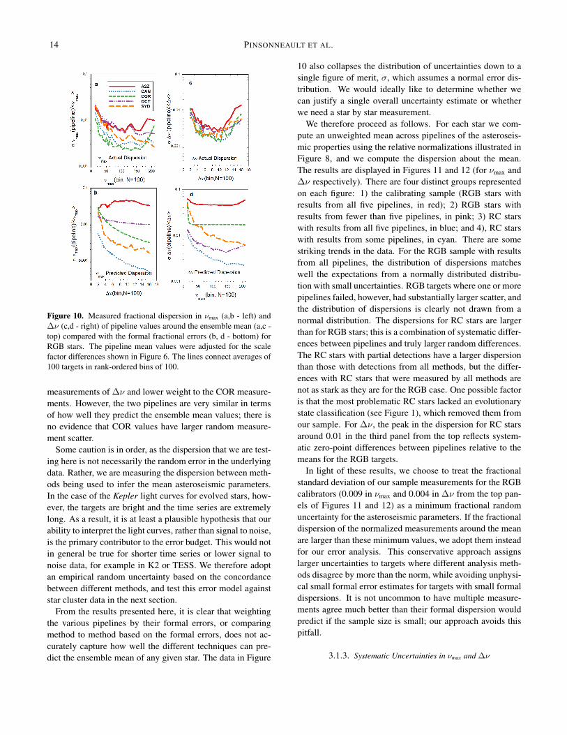
Our treatment of the random uncertainties represents an-other significant change in the model. Prior work has usedthe formal values returned by the pipelines as a measure ofrandom errors and combined these values with pipeline-to-pipeline differences in results to infer total error budgets.To test the pipeline error models, we compare the disper-sion of measurements from each pipeline around the normal-ized mean to the dispersion that would have been predictedby the formal pipeline uncertainties. In effect, this is test-ing whether the pipeline uncertainties behave as one wouldexpect for random error sources, i.e. that they reflect howwell the given method predicts the average measurements re-turned by all analysis techniques. The results are presented inFigure 10 (for νmax on the left and for ∆ν on the right). Twofeatures become immediately obvious: 1) the pipelines usu-ally (but not always) predict uncertainties much larger thanthe observed method to method differences; 2) there is noclear mapping between the formal predicted uncertainties forthe different pipelines and their true scatter around the en-semble mean. To take a concrete example, if we were touse the pipeline-predicted uncertainties in an error-weightedmean, we would have assigned very high weight to the CAN
14 PINSONNEAULT ET AL.
Figure 10. Measured fractional dispersion in νmax (a,b - left) and∆ν (c,d - right) of pipeline values around the ensemble mean (a,c -top) compared with the formal fractional errors (b, d - bottom) forRGB stars. The pipeline mean values were adjusted for the scalefactor differences shown in Figure 6. The lines connect averages of100 targets in rank-ordered bins of 100.
measurements of ∆ν and lower weight to the COR measure-ments. However, the two pipelines are very similar in termsof how well they predict the ensemble mean values; there isno evidence that COR values have larger random measure-ment scatter.
Some caution is in order, as the dispersion that we are test-ing here is not necessarily the random error in the underlyingdata. Rather, we are measuring the dispersion between meth-ods being used to infer the mean asteroseismic parameters.In the case of the Kepler light curves for evolved stars, how-ever, the targets are bright and the time series are extremelylong. As a result, it is at least a plausible hypothesis that ourability to interpret the light curves, rather than signal to noise,is the primary contributor to the error budget. This would notin general be true for shorter time series or lower signal tonoise data, for example in K2 or TESS. We therefore adoptan empirical random uncertainty based on the concordancebetween different methods, and test this error model againststar cluster data in the next section.
From the results presented here, it is clear that weightingthe various pipelines by their formal errors, or comparingmethod to method based on the formal errors, does not ac-curately capture how well the different techniques can pre-dict the ensemble mean of any given star. The data in Figure
10 also collapses the distribution of uncertainties down to asingle figure of merit, σ, which assumes a normal error dis-tribution. We would ideally like to determine whether wecan justify a single overall uncertainty estimate or whetherwe need a star by star measurement.
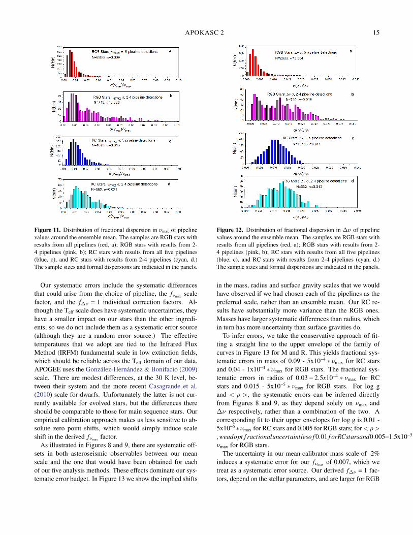
We therefore proceed as follows. For each star we com-pute an unweighted mean across pipelines of the asteroseis-mic properties using the relative normalizations illustrated inFigure 8, and we compute the dispersion about the mean.The results are displayed in Figures 11 and 12 (for νmax and∆ν respectively). There are four distinct groups representedon each figure: 1) the calibrating sample (RGB stars withresults from all five pipelines, in red); 2) RGB stars withresults from fewer than five pipelines, in pink; 3) RC starswith results from all five pipelines, in blue; and 4), RC starswith results from some pipelines, in cyan. There are somestriking trends in the data. For the RGB sample with resultsfrom all pipelines, the distribution of dispersions matcheswell the expectations from a normally distributed distribu-tion with small uncertainties. RGB targets where one or morepipelines failed, however, had substantially larger scatter, andthe distribution of dispersions is clearly not drawn from anormal distribution. The dispersions for RC stars are largerthan for RGB stars; this is a combination of systematic differ-ences between pipelines and truly larger random differences.The RC stars with partial detections have a larger dispersionthan those with detections from all methods, but the differ-ences with RC stars that were measured by all methods arenot as stark as they are for the RGB case. One possible factoris that the most problematic RC stars lacked an evolutionarystate classification (see Figure 1), which removed them fromour sample. For ∆ν, the peak in the dispersion for RC starsaround 0.01 in the third panel from the top reflects system-atic zero-point differences between pipelines relative to themeans for the RGB targets.
In light of these results, we choose to treat the fractionalstandard deviation of our sample measurements for the RGBcalibrators (0.009 in νmax and 0.004 in ∆ν from the top pan-els of Figures 11 and 12) as a minimum fractional randomuncertainty for the asteroseismic parameters. If the fractionaldispersion of the normalized measurements around the meanare larger than these minimum values, we adopt them insteadfor our error analysis. This conservative approach assignslarger uncertainties to targets where different analysis meth-ods disagree by more than the norm, while avoiding unphysi-cal small formal error estimates for targets with small formaldispersions. It is not uncommon to have multiple measure-ments agree much better than their formal dispersion wouldpredict if the sample size is small; our approach avoids thispitfall.
3.1.3. Systematic Uncertainties in νmax and ∆ν
APOKASC 2 15
Figure 11. Distribution of fractional dispersion in νmax of pipelinevalues around the ensemble mean. The samples are RGB stars withresults from all pipelines (red, a); RGB stars with results from 2-4 pipelines (pink, b); RC stars with results from all five pipelines(blue, c), and RC stars with results from 2-4 pipelines (cyan, d.)The sample sizes and formal dispersions are indicated in the panels.
Our systematic errors include the systematic differencesthat could arise from the choice of pipeline, the fνmax scalefactor, and the f∆ν = 1 individual correction factors. Al-though the Teff scale does have systematic uncertainties, theyhave a smaller impact on our stars than the other ingredi-ents, so we do not include them as a systematic error source(although they are a random error source.) The effectivetemperatures that we adopt are tied to the Infrared FluxMethod (IRFM) fundamental scale in low extinction fields,which should be reliable across the Teff domain of our data.APOGEE uses the González-Hernández & Bonifacio (2009)scale. There are modest differences, at the 30 K level, be-tween their system and the more recent Casagrande et al.(2010) scale for dwarfs. Unfortunately the latter is not cur-rently available for evolved stars, but the differences thereshould be comparable to those for main sequence stars. Ourempirical calibration approach makes us less sensitive to ab-solute zero point shifts, which would simply induce scaleshift in the derived fνmax factor.
As illustrated in Figures 8 and 9, there are systematic off-sets in both asteroseismic observables between our meanscale and the one that would have been obtained for eachof our five analysis methods. These effects dominate our sys-tematic error budget. In Figure 13 we show the implied shifts
Figure 12. Distribution of fractional dispersion in ∆ν of pipelinevalues around the ensemble mean. The samples are RGB stars withresults from all pipelines (red, a); RGB stars with results from 2-4 pipelines (pink, b); RC stars with results from all five pipelines(blue, c), and RC stars with results from 2-4 pipelines (cyan, d.)The sample sizes and formal dispersions are indicated in the panels.
in the mass, radius and surface gravity scales that we wouldhave observed if we had chosen each of the pipelines as thepreferred scale, rather than an ensemble mean. Our RC re-sults have substantially more variance than the RGB ones.Masses have larger systematic differences than radius, whichin turn has more uncertainty than surface gravities do.
To infer errors, we take the conservative approach of fit-ting a straight line to the upper envelope of the family ofcurves in Figure 13 for M and R. This yields fractional sys-tematic errors in mass of 0.09 - 5x10⁻⁴ ∗ νmax for RC starsand 0.04 - 1x10⁻⁴ ∗ νmax for RGB stars. The fractional sys-tematic errors in radius of 0.03 − 2.5x10⁻⁴ ∗ νmax for RCstars and 0.015 - 5x10⁻⁵ ∗ νmax for RGB stars. For log gand < ρ >, the systematic errors can be inferred directlyfrom Figures 8 and 9, as they depend solely on νmax and∆ν respectively, rather than a combination of the two. Acorresponding fit to their upper envelopes for log g is 0.01 -5x10⁻⁵∗νmax for RC stars and 0.005 for RGB stars; for<ρ>,weadopt f ractionaluncertaintieso f 0.01 f orRCstarsand0.005−1.5x10⁻⁵∗νmax for RGB stars.
The uncertainty in our mean calibrator mass scale of 2%induces a systematic error for our fνmax of 0.007, which wetreat as a systematic error source. Our derived f∆ν = 1 fac-tors, depend on the stellar parameters, and are larger for RGB
16 PINSONNEAULT ET AL.
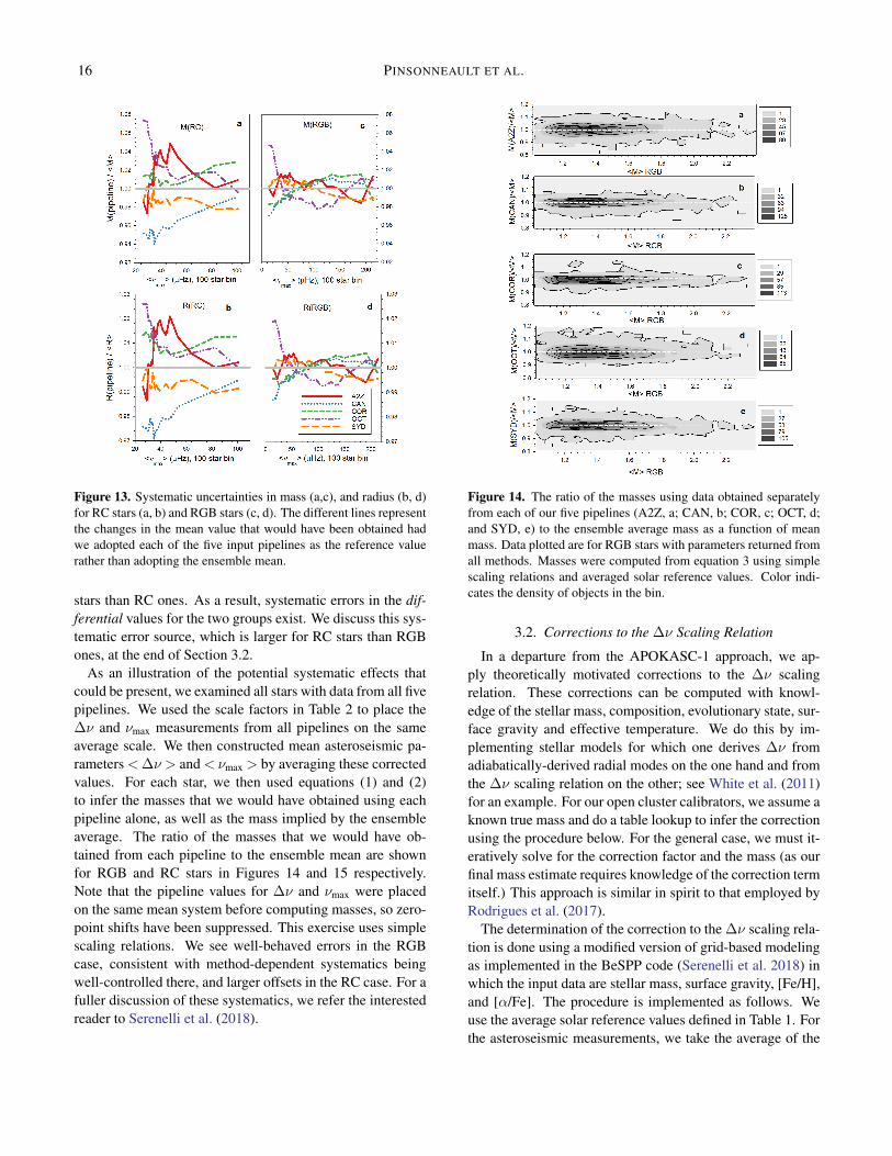
Figure 13. Systematic uncertainties in mass (a,c), and radius (b, d)for RC stars (a, b) and RGB stars (c, d). The different lines representthe changes in the mean value that would have been obtained hadwe adopted each of the five input pipelines as the reference valuerather than adopting the ensemble mean.
stars than RC ones. As a result, systematic errors in the dif-ferential values for the two groups exist. We discuss this sys-tematic error source, which is larger for RC stars than RGBones, at the end of Section 3.2.
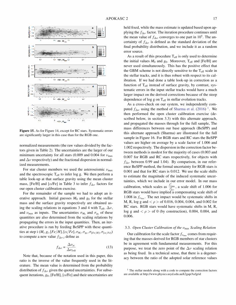
As an illustration of the potential systematic effects thatcould be present, we examined all stars with data from all fivepipelines. We used the scale factors in Table 2 to place the∆ν and νmax measurements from all pipelines on the sameaverage scale. We then constructed mean asteroseismic pa-rameters <∆ν > and < νmax > by averaging these correctedvalues. For each star, we then used equations (1) and (2)to infer the masses that we would have obtained using eachpipeline alone, as well as the mass implied by the ensembleaverage. The ratio of the masses that we would have ob-tained from each pipeline to the ensemble mean are shownfor RGB and RC stars in Figures 14 and 15 respectively.Note that the pipeline values for ∆ν and νmax were placedon the same mean system before computing masses, so zero-point shifts have been suppressed. This exercise uses simplescaling relations. We see well-behaved errors in the RGBcase, consistent with method-dependent systematics beingwell-controlled there, and larger offsets in the RC case. For afuller discussion of these systematics, we refer the interestedreader to Serenelli et al. (2018).
Figure 14. The ratio of the masses using data obtained separatelyfrom each of our five pipelines (A2Z, a; CAN, b; COR, c; OCT, d;and SYD, e) to the ensemble average mass as a function of meanmass. Data plotted are for RGB stars with parameters returned fromall methods. Masses were computed from equation 3 using simplescaling relations and averaged solar reference values. Color indi-cates the density of objects in the bin.
3.2. Corrections to the ∆ν Scaling Relation
In a departure from the APOKASC-1 approach, we ap-ply theoretically motivated corrections to the ∆ν scalingrelation. These corrections can be computed with knowl-edge of the stellar mass, composition, evolutionary state, sur-face gravity and effective temperature. We do this by im-plementing stellar models for which one derives ∆ν fromadiabatically-derived radial modes on the one hand and fromthe ∆ν scaling relation on the other; see White et al. (2011)for an example. For our open cluster calibrators, we assume aknown true mass and do a table lookup to infer the correctionusing the procedure below. For the general case, we must it-eratively solve for the correction factor and the mass (as ourfinal mass estimate requires knowledge of the correction termitself.) This approach is similar in spirit to that employed byRodrigues et al. (2017).
The determination of the correction to the ∆ν scaling rela-tion is done using a modified version of grid-based modelingas implemented in the BeSPP code (Serenelli et al. 2018) inwhich the input data are stellar mass, surface gravity, [Fe/H],and [α/Fe]. The procedure is implemented as follows. Weuse the average solar reference values defined in Table 1. Forthe asteroseismic measurements, we take the average of the
APOKASC 2 17
Figure 15. As for Figure 14, except for RC stars. Systematic errorsare significantly larger in this case than for the RGB one.
normalized measurements (the raw values divided by the fac-tors given in Table 2). The uncertainties are the larger of ourminimum uncertainty for all stars (0.009 and 0.004 for νmax
and ∆ν respectively) and the fractional dispersion in normal-ized measurements.
For star cluster members we used the asteroseismic νmax
and the spectroscopic Teff to infer log g. We then perform atable look-up at that surface gravity using the mean clustermass, [Fe/H] and [α/Fe] in Table 3 to infer f∆ν factors forour open cluster calibration exercise.
For the remainder of the sample we had to adopt an it-erative approach. Initial guesses M0 and g0 for the stellarmass and the surface gravity respectively are obtained us-ing the scaling relations in equations 3 and 4 with Teff, ∆ν,and νmax as inputs. The uncertainties σM0 and σg0 of thesequantities are also determined from the scaling relations bypropagating the errors in the input quantities. Then, an iter-ative procedure is run by feeding BeSPP with these quanti-ties at step i (Mi,gi, [Fe/H], [α/Fe],σMi ,σg0 ,σ[Fe/H],σ[α/Fe])to compute a new value f∆ν,i define as
f∆ν =∆νsc
∆νl=0(13)
Note that, because of the notation used in this paper, thisratio is the inverse of the value frequently used in the lit-erature. The mean value is determined from the probabilitydistribution of f∆ν given the quoted uncertainties. For subse-quent iterations, g0, [Fe/H], [α/Fe] and their uncertainties are
held fixed, while the mass estimate is updated based upon ap-plying the f∆ν factor. The iteration procedure continues untilthe mean value of f∆ν converges to one part in 105. The un-certainty of f∆ν is defined as the standard deviation of thefinal probability distribution, and we include it as a randomerror source.
As a result of this procedure Teff is only used to determinethe initial values M0 and g0. Moreover, Teff and [Fe/H] arenever used simultaneously. This has the positive effect thatthe GBM scheme is not directly sensitive to the Teff scale inthe stellar tracks, and it is thus robust with respect to its cal-ibration. If we had done a table look-up in correction as afunction of Teff instead of surface gravity, by contrast, sys-tematic errors in the input stellar tracks would have a muchlarger impact on the derived corrections because of the steepdependence of log g on Teff in stellar evolution tracks.
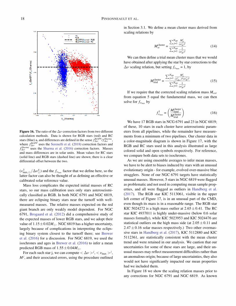
As a cross-check on our system, we independently com-puted f∆ν using the method of Sharma et al. (2016) 1. Wethen performed the open cluster calibration exercise (de-scribed below, in section 3.3) with this alternate approach,and propagated the masses through for the full sample, Themass differences between our base approach (BeSPP) andthis alternate approach (Sharma) are illustrated for the fullsample in Figure 16. For RGB stars and RC stars the BeSPPvalues are higher on average by a scale factor of 1.006 and1.002 respectively. The dispersion in the correction factor be-tween methods is modest for the majority of cases (0.003 and0.007 for RGB and RC stars respectively, for objects withf∆ν between 0.99 and 1.04). By comparison, in our refer-ence BeSPP method, the formal uncertainty for RGB stars is0.001 and that for RC stars is 0.012. We use the scale shiftsto estimate the magnitude of the induced systematic uncer-tainties, which we include in our error model. In our masscalibration, which scales as
f 3νmaxf 4∆ν
, a scale shift of 1.006 forRGB stars would have implied a compensating scale shift of1.008 in fνmax . The net impact would be systematic shifts inM, R, log g and < ρ > of 0.016, 0.004, 0.004, and 0.002 forRC stars. RGB stars would have systematic shifts in M, R,log g and < ρ > of 0 (by construction), 0.004, 0.004, and0.006.
3.3. Open Cluster Calibration of the νmax Scaling Relation
Our calibration for the scale factor fνmax comes from requir-ing that the masses derived for RGB members of star clustersbe in agreement with fundamental measurements. For thispurpose, we treat the zero point of the ∆ν scaling relationas being fixed. In a technical sense, that there is a degener-acy between the ratio of the adopted solar reference values
1 The stellar models along with a code to compute the correction factorsare available at http://www.physics.usyd.edu.au/k2gap/Asfgrid
18 PINSONNEAULT ET AL.
Figure 16. The ratio of the ∆ν correction factors from two differentcalculation methods. Data is shown for RGB stars (red) and RCstars (blue) a, and differences are defined in the sense f BeSPP
∆ν / f Sharma∆ν ,
where f BeSPP∆ν uses the Serenelli et al. (2018) correction factors and
f Sharma∆ν uses the Sharma et al. (2016) correction factors. Masses
and mass differences are in solar units. Mean values for RC stars(solid line) and RGB stars (dashed line) are shown; there is a cleardifferential offset between the two.
(ν3max,�/∆ν
4�) and the fνmax factor that we define here, so the
latter factor can also be thought of as defining an effective orcalibrated solar reference value.
Mass loss complicates the expected initial masses of RCstars, so our mass calibration uses only stars asteroseismi-cally classified as RGB. In both NGC 6791 and NGC 6819,there are eclipsing binary stars near the turnoff with well-measured masses. The relative masses expected on the redgiant branch are only weakly model dependent. For NGC6791, Brogaard et al. (2012) did a comprehensive study ofthe expected masses of lower RGB stars, and we adopt theirvalue of 1.15±0.02M�. NGC 6819 has a higher uncertainty,largely because of complications in interpreting the eclips-ing binary system closest to the turnoff there; see Breweret al. (2016) for a discussion. For NGC 6819, we used theisochrones and ages in Brewer et al. (2016) to infer a meanpredicted RGB mass of 1.55±0.04M�.
For each such star j, we can compute<∆ν > j, < νmax >j,
M j, and their associated errors, using the procedure outlined
in Section 3.1. We define a mean cluster mass derived fromscaling relations by
Mclustersc =
∑Nrgbj=1
M jsc
(σ jM )2∑Nrgb
j=11
(σ jM )2
(14)
We can then define a trial mean cluster mass that we wouldhave obtained after applying the star by star corrections to the∆ν scaling relation, but setting fνmax = 1, by
Mclustertrial =
∑Nrgbj=1
M jsc
( f j∆ν )4(σ j
M )2∑Nrgbj=1
1(σ j
M )2
(15)
If we require that the corrected scaling relation mass Mcor
from equation 5 equal the fundamental mass, we can thensolve for fνmax by
f 3νmax
=(
Mclusterfund
Mclustertrial
)(16)
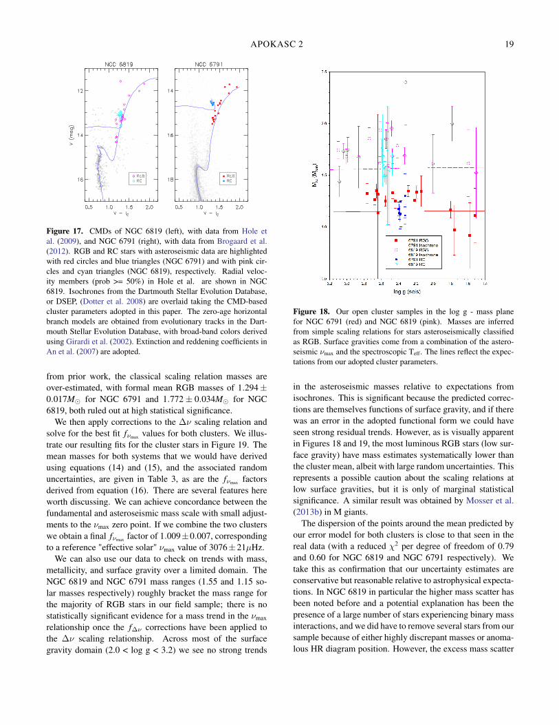
We have 17 RGB stars in NCG 6791 and 23 in NGC 6819;of these, 10 stars in each cluster have asteroseismic param-eters from all pipelines, while the remainder have measure-ments from a minimum of two pipelines. Our cluster data ina color-magnitude diagram is shown in Figure 17, with theRGB and RC stars used in this analysis illustrated as largecolored solid and open symbols respectively. For reference,we compare both data sets to isochrones.
As we are using ensemble averages to infer mean masses,we have to be alert to biases induced by stars with an unusualevolutionary origin - for example, evolved over-massive bluestragglers. None of our NGC 6791 targets have statisticallyunusual masses. However, 5 stars in NGC 6819 were flaggedas problematic and not used in computing mean sample prop-erties, and all were flagged as outliers in Handberg et al.(2017). The RGB star KIC 5113061, visible in the upperleft corner of Figure 17, is in an unusual part of the CMD,even though its mass is in a reasonable range. The RGB starKIC 5024272 is a high mass outlier at 2.65± 0.41. The RCstar KIC 4937011 is highly under-massive (below 0.6 solarmasses formally), while KIC 5023953 and KIC 5024476 arestatistical outliers on the high mass side (at 2.05± 0.11 and2.47± 0.16 solar masses respectively.) Two other overmas-sive stars in Handberg et al. (2017), KIC 5112880 and KIC5112361, are statistically consistent with the mean clustertrend and were retained in our analysis. We caution that ouruncertainties for some of these stars are large, and their un-usual masses may reflect measurement difficulties rather thanan anomalous origin; because of large uncertainties, they alsowould not have significantly impacted our mean propertieshad we included them.
In Figure 18 we show the scaling relation masses prior toany corrections for NGC 6791 and NGC 6819. As known
APOKASC 2 19
Figure 17. CMDs of NGC 6819 (left), with data from Hole etal. (2009), and NGC 6791 (right), with data from Brogaard et al.(2012). RGB and RC stars with asteroseismic data are highlightedwith red circles and blue triangles (NGC 6791) and with pink cir-cles and cyan triangles (NGC 6819), respectively. Radial veloc-ity members (prob >= 50%) in Hole et al. are shown in NGC6819. Isochrones from the Dartmouth Stellar Evolution Database,or DSEP, (Dotter et al. 2008) are overlaid taking the CMD-basedcluster parameters adopted in this paper. The zero-age horizontalbranch models are obtained from evolutionary tracks in the Dart-mouth Stellar Evolution Database, with broad-band colors derivedusing Girardi et al. (2002). Extinction and reddening coefficients inAn et al. (2007) are adopted.
from prior work, the classical scaling relation masses areover-estimated, with formal mean RGB masses of 1.294±0.017M� for NGC 6791 and 1.772± 0.034M� for NGC6819, both ruled out at high statistical significance.
We then apply corrections to the ∆ν scaling relation andsolve for the best fit fνmax values for both clusters. We illus-trate our resulting fits for the cluster stars in Figure 19. Themean masses for both systems that we would have derivedusing equations (14) and (15), and the associated randomuncertainties, are given in Table 3, as are the fνmax factorsderived from equation (16). There are several features hereworth discussing. We can achieve concordance between thefundamental and asteroseismic mass scale with small adjust-ments to the νmax zero point. If we combine the two clusterswe obtain a final fνmax factor of 1.009±0.007, correspondingto a reference "effective solar" νmax value of 3076±21µHz.
We can also use our data to check on trends with mass,metallicity, and surface gravity over a limited domain. TheNGC 6819 and NGC 6791 mass ranges (1.55 and 1.15 so-lar masses respectively) roughly bracket the mass range forthe majority of RGB stars in our field sample; there is nostatistically significant evidence for a mass trend in the νmax
relationship once the f∆ν corrections have been applied tothe ∆ν scaling relationship. Across most of the surfacegravity domain (2.0 < log g < 3.2) we see no strong trends
Figure 18. Our open cluster samples in the log g - mass planefor NGC 6791 (red) and NGC 6819 (pink). Masses are inferredfrom simple scaling relations for stars asteroseismically classifiedas RGB. Surface gravities come from a combination of the astero-seismic νmax and the spectroscopic Teff. The lines reflect the expec-tations from our adopted cluster parameters.
in the asteroseismic masses relative to expectations fromisochrones. This is significant because the predicted correc-tions are themselves functions of surface gravity, and if therewas an error in the adopted functional form we could haveseen strong residual trends. However, as is visually apparentin Figures 18 and 19, the most luminous RGB stars (low sur-face gravity) have mass estimates systematically lower thanthe cluster mean, albeit with large random uncertainties. Thisrepresents a possible caution about the scaling relations atlow surface gravities, but it is only of marginal statisticalsignificance. A similar result was obtained by Mosser et al.(2013b) in M giants.
The dispersion of the points around the mean predicted byour error model for both clusters is close to that seen in thereal data (with a reduced χ2 per degree of freedom of 0.79and 0.60 for NGC 6819 and NGC 6791 respectively). Wetake this as confirmation that our uncertainty estimates areconservative but reasonable relative to astrophysical expecta-tions. In NGC 6819 in particular the higher mass scatter hasbeen noted before and a potential explanation has been thepresence of a large number of stars experiencing binary massinteractions, and we did have to remove several stars from oursample because of either highly discrepant masses or anoma-lous HR diagram position. However, the excess mass scatter
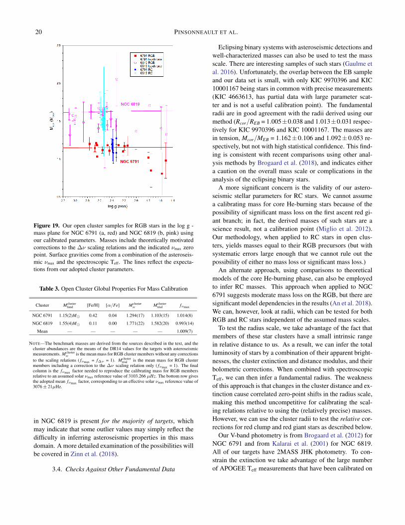
20 PINSONNEAULT ET AL.
Figure 19. Our open cluster samples for RGB stars in the log g -mass plane for NGC 6791 (a, red) and NGC 6819 (b, pink) usingour calibrated parameters. Masses include theoretically motivatedcorrections to the ∆ν scaling relations and the indicated νmax zeropoint. Surface gravities come from a combination of the asteroseis-mic νmax and the spectroscopic Teff. The lines reflect the expecta-tions from our adopted cluster parameters.
Table 3. Open Cluster Global Properties For Mass Calibration
Cluster Mclusterfund [Fe/H] [α/Fe] Mcluster
sc Mclustertrial fνmax
NGC 6791 1.15(2)M� 0.42 0.04 1.294(17) 1.103(15) 1.014(8)
NGC 6819 1.55(4)M� 0.11 0.00 1.771(22) 1.582(20) 0.993(14)
Mean — — — — — 1.009(7)
NOTE—The benchmark masses are derived from the sources described in the text, and thecluster abundances are the means of the DR14 values for the targets with asteroseismicmeasurements. Mcluster
sc is the mean mass for RGB cluster members without any correctionsto the scaling relations ( fνmax = f∆ν = 1). Mcluster
trial is the mean mass for RGB clustermembers including a correction to the ∆ν scaling relation only ( fνmax = 1). The finalcolumn is the fνmax factor needed to reproduce the calibrating mass for RGB membersrelative to an assumed solar νmax reference value of 3103.266 µHz. The bottom row givesthe adopted mean fνmax factor, corresponding to an effective solar νmax reference value of3076± 21µHz.
in NGC 6819 is present for the majority of targets, whichmay indicate that some outlier values may simply reflect thedifficulty in inferring asteroseismic properties in this massdomain. A more detailed examination of the possibilities willbe covered in Zinn et al. (2018).
3.4. Checks Against Other Fundamental Data
Eclipsing binary systems with asteroseismic detections andwell-characterized masses can also be used to test the massscale. There are interesting samples of such stars (Gaulme etal. 2016). Unfortunately, the overlap between the EB sampleand our data set is small, with only KIC 9970396 and KIC10001167 being stars in common with precise measurements(KIC 4663613, has partial data with large parameter scat-ter and is not a useful calibration point). The fundamentalradii are in good agreement with the radii derived using ourmethod (Rcor/REB = 1.005±0.038 and 1.013±0.031 respec-tively for KIC 9970396 and KIC 10001167. The masses arein tension, Mcor/MEB = 1.162±0.106 and 1.092±0.053 re-spectively, but not with high statistical confidence. This find-ing is consistent with recent comparisons using other anal-ysis methods by Brogaard et al. (2018), and indicates eithera caution on the overall mass scale or complications in theanalysis of the eclipsing binary stars.
A more significant concern is the validity of our astero-seismic stellar parameters for RC stars. We cannot assumea calibrating mass for core He-burning stars because of thepossibility of significant mass loss on the first ascent red gi-ant branch; in fact, the derived masses of such stars are ascience result, not a calibration point (Miglio et al. 2012).Our methodology, when applied to RC stars in open clus-ters, yields masses equal to their RGB precursors (but withsystematic errors large enough that we cannot rule out thepossibility of either no mass loss or significant mass loss.)
An alternate approach, using comparisons to theoreticalmodels of the core He-burning phase, can also be employedto infer RC masses. This approach when applied to NGC6791 suggests moderate mass loss on the RGB, but there aresignificant model dependencies in the results (An et al. 2018).We can, however, look at radii, which can be tested for bothRGB and RC stars independent of the assumed mass scales.
To test the radius scale, we take advantage of the fact thatmembers of these star clusters have a small intrinsic rangein relative distance to us. As a result, we can infer the totalluminosity of stars by a combination of their apparent bright-nesses, the cluster extinction and distance modulus, and theirbolometric corrections. When combined with spectroscopicTeff, we can then infer a fundamental radius. The weaknessof this approach is that changes in the cluster distance and ex-tinction cause correlated zero-point shifts in the radius scale,making this method uncompetitive for calibrating the scal-ing relations relative to using the (relatively precise) masses.However, we can use the cluster radii to test the relative cor-rections for red clump and red giant stars as described below.
Our V-band photometry is from Brogaard et al. (2012) forNGC 6791 and from Kalarai et al. (2001) for NGC 6819.All of our targets have 2MASS JHK photometry. To con-strain the extinction we take advantage of the large numberof APOGEE Teff measurements that have been calibrated on
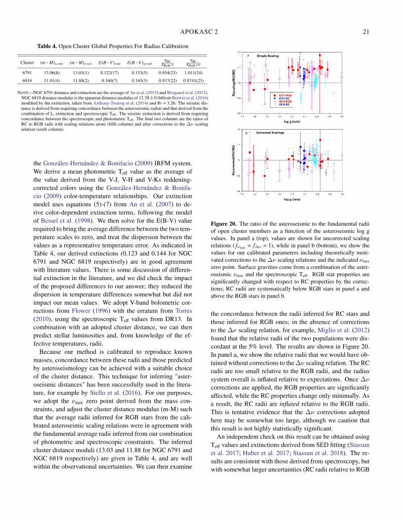
APOKASC 2 21
Table 4. Open Cluster Global Properties For Radius Calibration
Cluster (m − M)o,cmd (m − M)o,seis E(B −V )cmd E(B −V )sp+phRRC
RRGB ,scRRC
RRGB ,cor
6791 13.06(8) 13.03(1) 0.122(17) 0.153(5) 0.954(23) 1.011(24)
6819 11.91(4) 11.88(2) 0.160(7) 0.165(5) 0.917(22) 0.9741(23)
NOTE—NGC 6791 distance and extinction are the average of An et al. (2015) and Brogaard et al. (2012).NGC 6819 distance modulus is the apparent distance modulus of 12.38±0.04from Brewer et al. (2016)modified by the extinction, taken from Anthony-Twarog et al. (2014) and Rv = 3.26. The seismic dis-tance is derived from requiring concordance between the asteroseismic radius and that derived from thecombination of L, extinction and spectroscopic Teff. The seismic extinction is derived from requiringconcordance between the spectroscopic and photometric Teff. The final two columns are the ratios ofRC to RGB radii with scaling relations alone (fifth column) and after corrections to the ∆ν scalingrelation (sixth column).
the González-Hernández & Bonifacio (2009) IRFM system.We derive a mean photometric Teff value as the average ofthe value derived from the V-J, V-H and V-Ks reddening-corrected colors using the González-Hernández & Bonifa-cio (2009) color-temperature relationships. Our extinctionmodel uses equations (5)-(7) from An et al. (2007) to de-rive color-dependent extinction terms, following the modelof Bessel et al. (1998). We then solve for the E(B-V) valuerequired to bring the average difference between the two tem-perature scales to zero, and treat the dispersion between thevalues as a representative temperature error. As indicated inTable 4, our derived extinctions (0.123 and 0.144 for NGC6791 and NGC 6819 respectively) are in good agreementwith literature values. There is some discussion of differen-tial extinction in the literature, and we did check the impactof the proposed differences to our answer; they reduced thedispersion in temperature differences somewhat but did notimpact our mean values. We adopt V-band bolometric cor-rections from Flower (1996) with the erratum from Torres(2010), using the spectroscopic Teff values from DR13. Incombination with an adopted cluster distance, we can thenpredict stellar luminosities and, from knowledge of the ef-fective temperatures, radii.
Because our method is calibrated to reproduce knownmasses, concordance between these radii and those predictedby asteroseismology can be achieved with a suitable choiceof the cluster distance. This technique for inferring "aster-oseismic distances" has been successfully used in the litera-ture, for example by Stello et al. (2016). For our purposes,we adopt the νmax zero point derived from the mass con-straints, and adjust the cluster distance modulus (m-M) suchthat the average radii inferred for RGB stars from the cali-brated asteroseimic scaling relations were in agreement withthe fundamental average radii inferred from our combinationof photometric and spectroscopic constraints. The inferredcluster distance moduli (13.03 and 11.88 for NGC 6791 andNGC 6819 respectively) are given in Table 4, and are wellwithin the observational uncertainties. We can then examine
Figure 20. The ratio of the asteroseismic to the fundamental radiiof open cluster members as a function of the asteroseismic log gvalues. In panel a (top), values are shown for uncorrected scalingrelations ( fνmax = f∆ν = 1), while in panel b (bottom), we show thevalues for our calibrated parameters including theoretically moti-vated corrections to the ∆ν scaling relations and the indicated νmax
zero point. Surface gravities come from a combination of the aster-oseismic νmax and the spectroscopic Teff. RGB star properties aresignificantly changed with respect to RC properties by the correc-tions; RC radii are systematically below RGB stars in panel a andabove the RGB stars in panel b.
the concordance between the radii inferred for RC stars andthose inferred for RGB ones; in the absence of correctionsto the ∆ν scaling relation, for example, Miglio et al. (2012)found that the relative radii of the two populations were dis-cordant at the 5% level. The results are shown in Figure 20.In panel a, we show the relative radii that we would have ob-tained without corrections to the ∆ν scaling relation. The RCradii are too small relative to the RGB radii, and the radiussystem overall is inflated relative to expectations. Once ∆ν
corrections are applied, the RGB properties are significantlyaffected, while the RC properties change only minimally. Asa result, the RC radii are inflated relative to the RGB radii.This is tentative evidence that the ∆ν corrections adoptedhere may be somewhat too large, although we caution thatthis result is not highly statistically significant.
An independent check on this result can be obtained usingTeff values and extinctions derived from SED fitting (Stassunet al. 2017; Huber et al. 2017; Stassun et al. 2018). The re-sults are consistent with those derived from spectroscopy, butwith somewhat larger uncertainties (RC radii relative to RGB
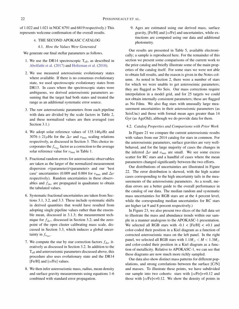
22 PINSONNEAULT ET AL.
of 1.022 and 1.021 in NGC 6791 and 6819 respectively.) Thisrepresents welcome confirmation of the overall results.
4. THE SECOND APOKASC CATALOG
4.1. How the Values Were Generated
We generate our final stellar parameters as follows.
1. We use the DR14 spectroscopic Teff, as described inAbolfathi et al. (2017) and Holtzman et al. (2018).
2. We use measured asteroseismic evolutionary stateswhere available. If there is no consensus evolutionarystate, we used spectroscopic evolutionary states fromDR13. In cases where the spectroscopic states wereambiguous, we derived asteroseismic parameters as-suming that the target had both states and treated therange as an additional systematic error source.
3. The raw asteroseismic parameters from each pipelinewith data are divided by the scale factors in Table 2,and these normalized values are then averaged (seeSection 3.1.)
4. We adopt solar reference values of 135.146µHz and3076± 21µHz for the ∆ν and νmax scaling relationsrespectively, as discussed in Section 3. This choice in-corporates the fνmax factor as a correction to the averagesolar reference value for νmax in Table 1.
5. Fractional random errors for asteroseismic observablesare taken as the larger of the normalized measurementdispersion σ(parameter)/<parameter> and our ’bestcase’ uncertainties (0.009 and 0.004 for νmax and ∆ν
respectively). Random uncertainties in these observ-ables and f∆ν are propagated in quadrature to obtainthe tabulated values.
6. Systematic fractional uncertainties are taken from Sec-tions 3.1, 3.2, and 3.3. These include systematic shiftsin derived quantities that would have resulted fromadopting single pipeline values rather than the ensem-ble mean, discussed in 3.1.3; the measurement tech-nique for f∆ν , discussed in Section 3.2; and the zero-point of the open cluster calibrating mass scale, dis-cussed in Section 3.3, which induces a global uncer-tainty in fνmax .
7. We compute the star by star correction factors f∆ν it-eratively as discussed in Section 3.2. In addition to theTeff and asteroseismic parameters discussed above, thisprocedure also uses evolutionary state and the DR14[Fe/H] and [α/Fe] values.
8. We then infer asteroseismic mass, radius, mean densityand surface gravity measurements using equations 1-6combined with standard error propagation.
9. Ages are estimated using our derived mass, surfacegravity, [Fe/H] and [α/Fe] and uncertainties, while ex-tinctions are computed using our data and additionalphotometry.
Our results are presented in Table 5, available electroni-cally; a sample is reproduced here. For the remainder of thissection we present some comparisons of the current work tothe prior catalog and briefly illustrate some of the main prop-erties of the catalog itself. For some stars we were not ableto obtain full results, and the reason is given in the Notes col-umn. As noted in Section 2, there were a number of starsfor which we were unable to get asteroseimic parameters;they are flagged as No Seis. Our mass corrections requireinterpolation in a model grid, and for 25 targets we couldnot obtain internally consistent parameters; these are flaggedas No Fdnu. We also flag stars with unusually large mea-surement uncertainties in their asteroseismic parameters (asSeisUnc) and those with formal mean ages greater than 14Gyr (as AgeOld), although we do provide data for them.
4.2. Catalog Properties and Comparisons with Prior Work
In Figure 21 we compare the current asteroseismic resultswith values from our 2014 catalog for stars in common. Forthe asteroseismic parameters, surface gravities are very well-behaved, and for the large majority of cases the changes inthe inferred ∆ν and νmax are small. We see some excessscatter for RC stars and a handful of cases where the meanparameters changed significantly between the two efforts.
Our distributions of uncertainties are illustrated in Figure22. The error distribution is skewed, with the high scattercases corresponding to the high uncertainty tails in the mea-surements of the asteroseismic parameters. As a result, me-dian errors are a better guide to the overall performance inthe catalog of our data. The median random and systematicmass uncertainties for RGB stars are at the 4 percent level,while the corresponding median uncertainties for RC starsare higher (at 9 and 8 percent respectively.)
In Figure 23, we also present two slices of the full data setto illustrate the mass and abundance trends within our sam-ple in a manner analogous to the APOKASC-1 presentation.We selected all RGB stars with -0.1 < [Fe/H] < +0.1 andcolor-coded their position in a Kiel diagram as a function ofcorrected asteroseismic mass on the left panel. In the rightpanel, we selected all RGB stars with 1.1M� < M < 1.3M�and color-coded their position in a Kiel diagram as a func-tion of metallicity. Relative to APOKASC-1, we can see thatthese diagrams are now much more richly sampled.
Our data also show distinct mass patterns for different pop-ulations, and strong correlations between the surface [C/N]and masses. To illustrate these points, we have subdividedour sample into two cohorts: stars with [α/Fe]>+0.12 andthose with [α/Fe]<+0.12. We show the density of points in
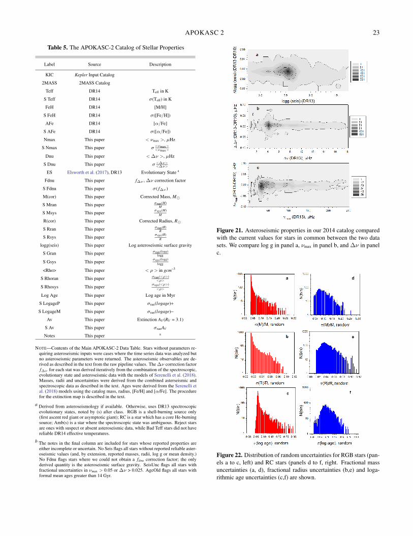
APOKASC 2 23
Table 5. The APOKASC-2 Catalog of Stellar Properties
Label Source Description
KIC Kepler Input Catalog
2MASS 2MASS Catalog
Teff DR14 Teff in K
S Teff DR14 σ(Teff) in K
FeH DR14 [M/H]
S FeH DR14 σ([Fe/H])
AFe DR14 [α/Fe]
S AFe DR14 σ([α/Fe])
Nmax This paper < νmax >, µHz
S Nmax This paper σ <νmax><νmax>
Dnu This paper <∆ν >, µHz
S Dnu This paper σ <∆ν><∆ν>
ES Elsworth et al. (2017), DR13 Evolutionary State a
Fdnu This paper f∆ν , ∆ν correction factor
S Fdnu This paper σ( f∆ν )
M(cor) This paper Corrected Mass, M�
S Mran This paper σran(M)M
S Msys This paperσsys(M)
M
R(cor) This paper Corrected Radius, R�
S Rran This paper σran(R)R
S Rsys This paperσsys(R)
R
logg(seis) This paper Log asteroseismic surface gravity
S Gran This paper σran(logg)logg
S Gsys This paperσsys(logg)
logg
<Rho> This paper < ρ > in gcm−3
S Rhoran This paper σran(<ρ>)<ρ>
S Rhosys This paperσsys(<ρ>)
<ρ>
Log Age This paper Log age in Myr
S LogageP This paper σran(logage)+
S LogageM This paper σran(logage)−
Av This paper Extinction AV (RV = 3.1)
S Av This paper σranAV
Notes This paper a
NOTE—Contents of the Main APOKASC-2 Data Table. Stars without parameters re-quiring asteroseismic inputs were cases where the time series data was analyzed butno asteroseismic parameters were returned. The asteroseismic observables are de-rived as described in the text from the raw pipeline values. The ∆ν correction factorf∆ν for each stat was derived iteratively from the combination of the spectroscopic,evolutionary state and asteroseismic data with the models of Serenelli et al. (2018).Masses, radii and uncertainties were derived from the combined asterseismic andspectroscopic data as described in the text. Ages were derived from the Serenelli etal. (2018) models using the catalog mass, radius, [Fe/H] and [α/Fe]. The procedurefor the extinction map is described in the text.
a Derived from asteroseismology if available. Otherwise, uses DR13 spectroscopicevolutionary states, noted by (s) after class. RGB is a shell-burning source only(first ascent red giant or asymptotic giant); RC is a star which has a core He-burningsource; Amb(s) is a star where the spectroscopic state was ambiguous. Reject starsare ones with suspect or absent asteroseismic data, while Bad Teff stars did not havereliable DR14 effective temperatures.
b The notes in the final column are included for stars whose reported properties areeither incomplete or uncertain. No Seis flags all stars without reported reliable aster-oseismic values (and, by extension, reported masses, radii, log g or mean density.)No Fdnu flags stars where we could not obtain a fdnu correction factor; the onlyderived quantity is the asteroseismic surface gravity. SeisUnc flags all stars withfractional uncertainties in νmax > 0.05 or ∆ν > 0.025. AgeOld flags all stars withformal mean ages greater than 14 Gyr.
Figure 21. Asteroseismic properties in our 2014 catalog comparedwith the current values for stars in common between the two datasets. We compare log g in panel a, νmax in panel b, and ∆ν in panelc.
Figure 22. Distribution of random uncertainties for RGB stars (pan-els a to c, left) and RC stars (panels d to f, right. Fractional massuncertainties (a, d), fractional radius uncertainties (b,e) and loga-rithmic age uncertainties (c,f) are shown.
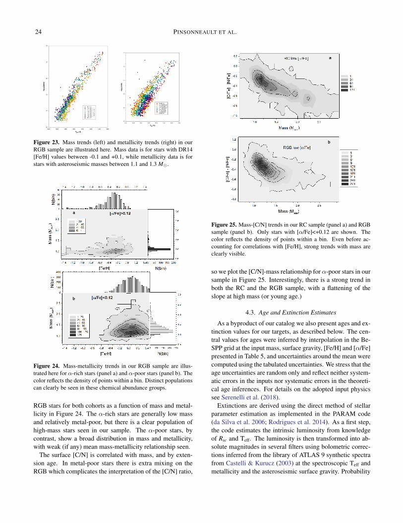
24 PINSONNEAULT ET AL.
Figure 23. Mass trends (left) and metallicity trends (right) in ourRGB sample are illustrated here. Mass data is for stars with DR14[Fe/H] values between -0.1 and +0.1, while metallicity data is forstars with asteroseismic masses between 1.1 and 1.3 M�.
Figure 24. Mass-metallicity trends in our RGB sample are illus-trated here for α-rich stars (panel a) and α-poor stars (panel b). Thecolor reflects the density of points within a bin. Distinct populationscan clearly be seen in these chemical abundance groups.
RGB stars for both cohorts as a function of mass and metal-licity in Figure 24. The α-rich stars are generally low massand relatively metal-poor, but there is a clear population ofhigh-mass stars seen in our sample. The α-poor stars, bycontrast, show a broad distribution in mass and metallicity,with weak (if any) mean mass-metallicity relationship seen.
The surface [C/N] is correlated with mass, and by exten-sion age. In metal-poor stars there is extra mixing on theRGB which complicates the interpretation of the [C/N] ratio,
Figure 25. Mass-[C/N] trends in our RC sample (panel a) and RGBsample (panel b). Only stars with [α/Fe]<+0.12 are shown. Thecolor reflects the density of points within a bin. Even before ac-counting for correlations with [Fe/H], strong trends with mass areclearly visible.
so we plot the [C/N]-mass relationship for α-poor stars in oursample in Figure 25. Interestingly, there is a strong trend inboth the RC and the RGB sample, with a flattening of theslope at high mass (or young age.)
4.3. Age and Extinction Estimates
As a byproduct of our catalog we also present ages and ex-tinction values for our targets, as described below. The cen-tral values for ages were inferred by interpolation in the Be-SPP grid at the input mass, surface gravity, [Fe/H] and [α/Fe]presented in Table 5, and uncertainties around the mean werecomputed using the tabulated uncertainties. We stress that theage uncertainties are random only and reflect neither system-atic errors in the inputs nor systematic errors in the theoreti-cal age inferences. For details on the adopted input physicssee Serenelli et al. (2018).
Extinctions are derived using the direct method of stellarparameter estimation as implemented in the PARAM code(da Silva et al. 2006; Rodrigues et al. 2014). As a first step,the code estimates the intrinsic luminosity from knowledgeof Rsc and Teff. The luminosity is then transformed into ab-solute magnitudes in several filters using bolometric correc-tions inferred from the library of ATLAS 9 synthetic spectrafrom Castelli & Kurucz (2003) at the spectroscopic Teff andmetallicity and the asteroseismic surface gravity. Probability
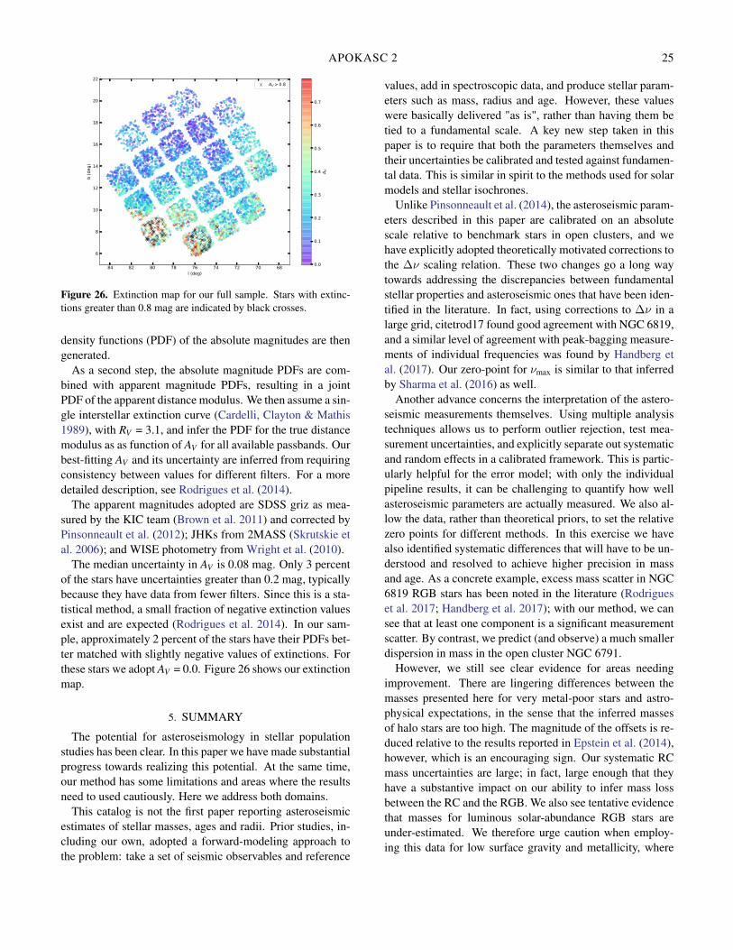
APOKASC 2 25
687072747678808284l (deg)
6
8
10
12
14
16
18
20
22
b (d
eg)
AV > 0.8
0.0
0.1
0.2
0.3
0.4
0.5
0.6
0.7
A V
Figure 26. Extinction map for our full sample. Stars with extinc-tions greater than 0.8 mag are indicated by black crosses.
density functions (PDF) of the absolute magnitudes are thengenerated.
As a second step, the absolute magnitude PDFs are com-bined with apparent magnitude PDFs, resulting in a jointPDF of the apparent distance modulus. We then assume a sin-gle interstellar extinction curve (Cardelli, Clayton & Mathis1989), with RV = 3.1, and infer the PDF for the true distancemodulus as as function of AV for all available passbands. Ourbest-fitting AV and its uncertainty are inferred from requiringconsistency between values for different filters. For a moredetailed description, see Rodrigues et al. (2014).
The apparent magnitudes adopted are SDSS griz as mea-sured by the KIC team (Brown et al. 2011) and corrected byPinsonneault et al. (2012); JHKs from 2MASS (Skrutskie etal. 2006); and WISE photometry from Wright et al. (2010).
The median uncertainty in AV is 0.08 mag. Only 3 percentof the stars have uncertainties greater than 0.2 mag, typicallybecause they have data from fewer filters. Since this is a sta-tistical method, a small fraction of negative extinction valuesexist and are expected (Rodrigues et al. 2014). In our sam-ple, approximately 2 percent of the stars have their PDFs bet-ter matched with slightly negative values of extinctions. Forthese stars we adopt AV = 0.0. Figure 26 shows our extinctionmap.
5. SUMMARY
The potential for asteroseismology in stellar populationstudies has been clear. In this paper we have made substantialprogress towards realizing this potential. At the same time,our method has some limitations and areas where the resultsneed to used cautiously. Here we address both domains.
This catalog is not the first paper reporting asteroseismicestimates of stellar masses, ages and radii. Prior studies, in-cluding our own, adopted a forward-modeling approach tothe problem: take a set of seismic observables and reference
values, add in spectroscopic data, and produce stellar param-eters such as mass, radius and age. However, these valueswere basically delivered "as is", rather than having them betied to a fundamental scale. A key new step taken in thispaper is to require that both the parameters themselves andtheir uncertainties be calibrated and tested against fundamen-tal data. This is similar in spirit to the methods used for solarmodels and stellar isochrones.
Unlike Pinsonneault et al. (2014), the asteroseismic param-eters described in this paper are calibrated on an absolutescale relative to benchmark stars in open clusters, and wehave explicitly adopted theoretically motivated corrections tothe ∆ν scaling relation. These two changes go a long waytowards addressing the discrepancies between fundamentalstellar properties and asteroseismic ones that have been iden-tified in the literature. In fact, using corrections to ∆ν in alarge grid, citetrod17 found good agreement with NGC 6819,and a similar level of agreement with peak-bagging measure-ments of individual frequencies was found by Handberg etal. (2017). Our zero-point for νmax is similar to that inferredby Sharma et al. (2016) as well.
Another advance concerns the interpretation of the astero-seismic measurements themselves. Using multiple analysistechniques allows us to perform outlier rejection, test mea-surement uncertainties, and explicitly separate out systematicand random effects in a calibrated framework. This is partic-ularly helpful for the error model; with only the individualpipeline results, it can be challenging to quantify how wellasteroseismic parameters are actually measured. We also al-low the data, rather than theoretical priors, to set the relativezero points for different methods. In this exercise we havealso identified systematic differences that will have to be un-derstood and resolved to achieve higher precision in massand age. As a concrete example, excess mass scatter in NGC6819 RGB stars has been noted in the literature (Rodrigueset al. 2017; Handberg et al. 2017); with our method, we cansee that at least one component is a significant measurementscatter. By contrast, we predict (and observe) a much smallerdispersion in mass in the open cluster NGC 6791.
However, we still see clear evidence for areas needingimprovement. There are lingering differences between themasses presented here for very metal-poor stars and astro-physical expectations, in the sense that the inferred massesof halo stars are too high. The magnitude of the offsets is re-duced relative to the results reported in Epstein et al. (2014),however, which is an encouraging sign. Our systematic RCmass uncertainties are large; in fact, large enough that theyhave a substantive impact on our ability to infer mass lossbetween the RC and the RGB. We also see tentative evidencethat masses for luminous solar-abundance RGB stars areunder-estimated. We therefore urge caution when employ-ing this data for low surface gravity and metallicity, where
26 PINSONNEAULT ET AL.
we lack direct calibrators. We have only limited constraintson the functional form of corrections to the ∆ν scaling re-lation as well, and different methods have been proposed inthe literature; even within a calibrated framework, this couldyield systematic changes that are not captured by our currentapproach. Similarly, identifying the origin of the method-dependent differences in asteroseismic measurements is animportant task and could yield more precise relative and ab-solute stellar parameters.
The empirical approach here does not include grid-modeling constraints from stellar tracks, and as a result thereare objects included here with implausible combinations ofmass, log g, Teff, and abundance; the approach in Serenelliet al. (2018) does a much better job of controlling for suchanomalies, at the cost of a dependence on the soundness ofthe underlying isochrones.
The most significant cautions about the usage of the cur-rent data are tied to the derived properties of red clump starsand selection effects in the underlying sample. There are sig-nificant method-dependent offsets in the asteroseismic mea-surements in red clump stars relative to first ascent red giants,and these effects are (if anything) amplified when grid mod-eling constraints are included. When combined with a lackof direct calibrators for their masses, we cannot rule out thepossibility of substantive zero-point shifts and stretches in therelative properties of such stars.
As documented in Pinsonneault et al. (2014), the selec-tion function for our sample is quite complex, and as a resultgreat care should be used before treating our mass distribu-tion as characteristic of the underlying population. An effortin preparation, including a more unbiased sample of spectro-scopic and asteroseismic data, will help alleviate the selec-tion effect problem. The forthcoming availability of preciseparallax constraints from Gaia may help provide calibrators,at least for radius, in red clump stars (in conjunction withwork on the extinction, bolometric correction, and effectivetemperature side.) Finally, improvements in the precisionand accurary of the spectroscopic parameters are also a re-alistic prospect.
We close on a note of optimism: although the emergingpicture is more complex than the simple adoption of scal-ing relations, we believe that it is now clear that asteroseis-mic masses (and associated ages) are astrophysically well-motivated, and that employing them for stellar populationstudies has a bright future.
MHP, JAJ, JT and JZ acknowledge support from NASAgrants NNX17AJ40G and NNX15AF13G. DA acknowl-edges support provided by the National Research Founda-tion of Korea (No. 2017R1A5A1070354). EC is funded bythe European Union’s Horizon 2020 research and innovationprogram under the Marie Sklodowska-Curie grant agreement
No.664931. YE acknowledges the support of the UK Scienceand Technology Facilities Council (STFC). K.C and V.S. ac-knowledge that their work here is supported in part by NASAunder grant 16-XRP16 2-0004, issued through the Astro-physics Division of the Science Mission Directorate. R.A.Gacknowledges support from CNES. A.G.H. acknowledgessupport from CNESDAGH and OZ acknowledge supportprovided by the Spanish Ministry of Economy and Com-petitiveness (MINECO) under grants AYA-2014-58082-Pand AYA-2017-88254-P. LG and TR acknowledge supportfrom PRIN INAF 2014 âAS CRA1.05.01.94.05. D.H. ac-knowledges support by NASA under Grant NNX14AB92Gissued through the Kepler Participating Scientist Program.HJ acknowledges support from the Crafoord Foundationand Stiftelsen Olle Engkvist Byggmästare. SK acknowl-edges support from the European Research Council underthe European Community’s Seventh Framework Programme(FP7/2007-2013) / ERC grant agreement no 338251 (Stel-larAges). SM acknowledges support from NASA grantNNX15AF13G and NSF grant AST-1411685 and the Ra-mon y Cajal fellowship number RYC-2015-17697. SzM hasbeen supported by the Premium Postdoctoral Research Pro-gram of the Hungarian Academy of Sciences, and by theHungarian NKFI Grants K-119517 of the Hungarian Na-tional Research, Development and Innovation Office. D.S isthe recipient of an Australian Research Council Future Fel-lowship (project number FT1400147). T.C.B. acknowledgespartial support from Grant No. PHY-1430152 (Physics Fron-tier Center/JINA Center for the Evolution of the Elements),awarded by the U.S. National Science Foundation.
Funding for the Sloan Digital Sky Survey IV has been pro-vided by the Alfred P. Sloan Foundation, the U.S. Depart-ment of Energy Office of Science, and the Participating Insti-tutions. SDSS-IV acknowledges support and resources fromthe Center for High-Performance Computing at the Univer-sity of Utah. The SDSS web site is www.sdss.org.
SDSS-IV is managed by the Astrophysical Research Con-sortium for the Participating Institutions of the SDSS Col-laboration including the Brazilian Participation Group, theCarnegie Institution for Science, Carnegie Mellon Univer-sity, the Chilean Participation Group, the French Participa-tion Group, Harvard-Smithsonian Center for Astrophysics,Instituto de Astrofísica de Canarias, The Johns Hopkins Uni-versity, Kavli Institute for the Physics and Mathematics ofthe Universe (IPMU) / University of Tokyo, Lawrence Berke-ley National Laboratory, Leibniz Institut für AstrophysikPotsdam (AIP), Max-Planck-Institut für Astronomie (MPIAHeidelberg), Max-Planck-Institut für Astrophysik (MPAGarching), Max-Planck-Institut für Extraterrestrische Physik(MPE), National Astronomical Observatories of China, NewMexico State University, New York University, Universityof Notre Dame, Observatário Nacional / MCTI, The Ohio
APOKASC 2 27
Table 6. Individual Asteroseismic Pipeline Measurements
Label Description
KEPLER ID Kepler Input Catalog ID
A2Z NUMAX A2Z Frequency of Maximum Power, µHz
A2Z NUMAXERR A2Z Frequency of Maximum Power Uncertainty, µHz
A2Z DELTANU A2Z Large Frequency Spacing, µHz
A2Z DELTANUERR A2Z Large Frequency Spacing Uncertainty, µHz
CAN NUMAX CAN Frequency of Maximum Power, µHz
CAN NUMAXERR CAN Frequency of Maximum Power Uncertainty, µHz
CAN DELTANU CAN Large Frequency Spacing, µHz
CAN DELTANUERR CAN Large Frequency Spacing Uncertainty, µHz
COR NUMAX COR Frequency of Maximum Power, µHz
COR NUMAXERR COR Frequency of Maximum Power Uncertainty, µHz
COR DELTANU COR Large Frequency Spacing, µHz
COR DELTANUERR COR Large Frequency Spacing Uncertainty, µHz
OCT NUMAX OCT Frequency of Maximum Power, µHz
OCT NUMAXERR OCT Frequency of Maximum Power Uncertainty, µHz
OCT DELTANU OCT Large Frequency Spacing, µHz
OCT DELTANUERR OCT Large Frequency Spacing Uncertainty, µHz
SYD NUMAX SYD Frequency of Maximum Power, µHz
SYD NUMAXERR SYD Frequency of Maximum Power Uncertainty, µHz
SYD DELTANU SYD Large Frequency Spacing, µHz
SYD DELTANUERR SYD Large Frequency Spacing Uncertainty, µHz
NOTE—individual pipeline values used in our analysis. The formal uncertainties re-turned by each analysis method are also given.
State University, Pennsylvania State University, ShanghaiAstronomical Observatory, United Kingdom ParticipationGroup, Universidad Nacional Autónoma de México, Univer-sity of Arizona, University of Colorado Boulder, University
of Oxford, University of Portsmouth, University of Utah,University of Virginia, University of Washington, Universityof Wisconsin, Vanderbilt University, and Yale University.
Facilities: Sloan, Kepler
APPENDIX
Our main catalog uses asteroseismic measurements from five distinct pipelines, and these values were combined as describedin Section 3.1; the averaged measurements and their computed uncertainties were given in Table 5. In Table 6 we present theindividual pipeline values used to compute the means and uncertainties.
REFERENCES
Silva Aguirre, V., Casagrande, L., Basu, S. et al. 2012 ApJ, 757, 99
Silva Aguirre, V., Bojsen-Hansen, M., Slumstrup, D. et al. 2017,MNRAS, in press
Abolfathi, B., Aguado, D. S., Aguilar, G. et al. 2017, ApJSupp, inpress
SDSS, Ahn, Christopher P., Alexandroff, Rachael, Allende Prieto,Carlos et al. 2010 ApJS211,17
SDSS, Albareti, Franco D.; Allende Prieto, Carlos; Almeida,Andres et al. 2017 submitted ApJS
Alvarez, R. & Plez, B. 1998, A&A, 330, 1109
An, Deokkeun, Terndrup, Donald M. & Pinsonneault, Marc H.2007, ApJ, 671, 1640
An, Deokkeun, Terndrup, Donald M., Pinsonneault, Marc H. &Lee, Jae-Woo 2015, ApJ, 811, 46
An, Deokkeun et al. 2018, in preparation
Anthony-Twarog, Barbara J., Deliyannis, Constantine P., Twarog,Bruce A. 2014 AJ, 148, 51
Asplund, M., Grevesse, N. & Sauval, A. J. 2005, ASPC, 336, 25
Beck, P. G., Montalban, J., Kallinger, T., et al. 2012, Nature, 481,55
28 PINSONNEAULT ET AL.
Bedding, T. R., Huber, D., Stello, D., et al. 2010, ApJL, 713, L176Bedding, Timothy R.; Mosser, Benoit; Huber, Daniel et al. 2011,
Nature, 471, 608Belkacem, K., Goupil, M. J., Dupret, M. A. et al. 2011, A&A, 530,
182Belkacem, K., Samadi, R., Mosser, B. et al. 2013, Progress in
Physics of the Sun and Stars: A New Era in Helio- andAsteroseismology. Proceedings of a Fujihara Seminar held 25-29November, 2012, in Hakone, Japan. Edited by H. Shibahashi andA.E. Lynas-Gray. ASP Conference Proceedings, Vol. 479. SanFrancisco: Astronomical Society of the Pacific, 2013., p.61
Bessell, M.S., Castelli, F. & Plez, B. 1998, A&A, 333, 231Blanton, Michael R., Bershady, Matthew A., Abolfathi, Bela et al.
2017, AJ, 154, 28Borucki, William J., Koch, David, Basri, Gibor et al. 2010,
Science, 327, 977Bossini, D., Miglio, A., Salaris, M. et al. 2017, MNRAS, 469, 4718Brewer, Lauren N., Sandquist, Eric L., Mathieu, Robert D. et al.
2016, AJ, 151, 66Brogaard, K., VandenBerg, D. A., Bruntt, H. et al. 2012, A&A,
543, 106Brogaard, K., Hansen, C. J., Miglio, A. et al. 2018, MNRAS, in
press.Brown T.M., Latham D. W., Everett M. E. & Esquerdo G. A. 2011,
AJ, 142, 112Cardelli J.A., Clayton G.C. & Mathis J. S. 1989, ApJ, 345, 245Casagrande, L., Ramírez, I., Meléndez, J., Bessell, M. & Asplund,
M. 2010, A&A, 512, 54Castelli F. & Kurucz R. L., 2003, in IAU Symposium, Vol. 210,
Modelling of Stellar Atmospheres, N. Piskunov, W. W. Weiss, &D. F. Gray, ed., p. 20.
Chiappini, C., Anders, F., Rodrigues, T. S. et al. 2015, A&A, 576,L12
Constantino, Thomas, Campbell, Simon W.,Christensen-Dalsgaard, JÃÿrgen et al. 2015, MNRAS, 452, 123
da Silva, L., Girardi, L., Pasquini, L. et al. 2006, A&A458, 609Deheuvels, S., GarcÂt’Äsa, R. A., Chaplin, W. J., et al. 2012, ApJ,
756, 19De Ridder, J., Barban, C., Baudin, F., et al. 2009, Nature, 459, 398Dotter, A., Chaboyer, B., Jevremovic, D., et al. 2008, ApJS, 178, 89Eisenstein, Daniel J., Weinberg, David H., Agol, Eric et al. 2011,
AJ, 142, 72Elsworth, Yvonne, Hekker, Saskia, Basu, Sarbani & Davies, Guy
R. 2017, MNRAS466, 3644Elsworth, Y. et al. 2018, submitted ApJEpstein, Courtney R., Elsworth, Yvonne P., Johnson, Jennifer A. et
al. 2015, ApJL, 785, L28Flower, P.J. 1996, ApJ, 469, 355Garcia, R.A., Hekker, S., Stello, D. et al. 2011, MNRAS, 414, L6Garcia, R., Mathur, S., Pires, S. et al. 2014, A&A, 568, 10
Garcia Pérez, Ana E.; Allende Prieto, Carlos; Holtzman, Jon A. etal. 2016, AJ, 151, 144
Gaulme, P., McKeever, J., Jackiewicz, J. et al. 2016, ApJ, 832, 121Girardi, L., Bertelli, G., Bressan, A., et al. 2002, A&A, 391, 195González Hernández, J. I. & Bonifacio, P. 2009, A&A, 497, 497Grevesse, N., & Sauval, A. J. 1998, SSR, 85, 161Gunn, James E., Siegmund, Walter A., Mannery, Edward J. et al.
2006, AJ, 131, 2332Handberg, R. & Lund, M.N. 2014, MNRAS, 445, 2698Handberg, R., Brogaard, K., Miglio, A. et al. 2017, MNRAS, 472,
979Hekker, S., Broomhall, A.-M., Chaplin, W. J. at al. 2010, MNRAS,
402, 2049Hekker, S., Elsworth, Y., De Ridder, J. et al. 2011, A&A, 525, 131Hekker, S., Elsworth, Y., Mosser, B. et al. 2012, A&A, 544, 90Hole, K. T., Geller, A. M., Mathieu, R. D., et al. 2009, AJ, 138, 159Holtzman, J. A., Shetrone, M., Johnson, J.A. et al. 2015, AJ, 150,
148Holtzman, J. et al. 2018, in preparationHuber, D., Stello, D., Bedding, T. R., et al. 2009, Commun.
Asteroseismol., 160, 74Huber, D., Ireland, M.J., Bedding, T.R. et al. 2012, ApJ, 760, 32Huber, Daniel, Zinn, Joel, Bojsen-Hansen, Mathias et al. 2017,
ApJ, 844, 122Izzard, Robert G., Preece, Holly, Jofre, Paula et al. 2018, MNRAS,
473, 2894Jofre, P., Jorissen, A., Van Eck, S. et al. 2016, A&A, 595, 60Jönsson, H., et al., in preparationKalirai, Jasonjot Singh, Richer, Harvey B., Fahlman, Gregory G. et
al. 2001, AJ, 122, 266Kallinger, T. et al. 2010, A&A, 522, 1Kjeldsen, H. & Bedding, T.R. 1995, A&A, 293, 87Li, Tanda, Bedding, Timothy R., Huber, Daniel et al. 2018,
MNRAS, 475, 981Majewski, Steven R., Schiavon, Ricardo P., Frinchaboy, Peter M. et
al. 2017, AJ, 154, 94Martig, M., Rix, H.-W., Silva Aguirre, V. et al. 2015, MNRAS,
451, 2230Martig, M., Fouesneau, M., Rix, H.-W., et al. 2016, MNRAS, 456,
3655Masseron, T., Lagarde, N., Miglio, A. et al. 2017, MNRAS, 464,
3021Mathur, S., GarcÄsa, R. A., Regulo, C., et al. 2010b, A&A, 511, 46Meszaros, Sz., Allende Prieto, C., Edvardsson, B. et al. 2012, AJ,
144, 120Meszaros, Sz., Holtzman, J., García Pérez, A. E. et al 2013, AJ,
146, 133Miglio, A.; Brogaard, K.; Stello, D. et al. 2012, MNRAS419, 2077Mosser, B. & Appourchaux, T. 2009, A&A, 508, 877Mosser, B. Michel, E., Belkacem, K. et al. 2013, A&A, 550, 126
APOKASC 2 29
Mosser, B., Dziembowski, W. A., Belkacem, K. et al. 2013, A&A,559, 137
Ness, M., Hogg, D. Rix, H.-W. et al. 2016, ApJ, 823, 114Nidever, David L., Holtzman, Jon A., Allende Prieto, Carlos et al.
2015, AJ, 150, 173Pinsonneault M. H., An D., Molenda-Zakowicz J. et al. 2012,
ApJS, 199, 30Pinsonneault, Marc H., Elsworth, Yvonne, Epstein, Courtney et al.
2014, ApJS215, 19Rodrigues, Thaíse S.; Girardi, Léo; Miglio, Andrea et al. 2014,
MNRAS, 445, 2758Rodrigues, Thaíse S.; Bossini, Diego; Miglio, Andrea et al. 2017,
MNRAS, 467, 1433Salaris, Maurizio; Pietrinferni, Adriano, Piersimoni, Anna M., &
Cassisi, Santi 2015, A&A, 583, 87Salaris, M., Cassisi, S., Schiavon, R. P. & Pietrinferni, A. 2018,
A&A, in press (astro-ph/180109441).Serenelli, A., Johnson, J., Huber, D. et al. 2017 ApJS233, 23Serenelli, A. et al. 2018, in prepSharma, Sanjib, Stello, Dennis, Bland-Hawthorn, Joss et al. 2016,
ApJ, 822, 15Shetrone, M., Bizyaev, D., Lawler, J. E. et al. 2015, ApJS, 221, 24Skrutskie, M. F., Cutri, R. M., Stiening, R. et al. 2006, AJ, 131,
1163
Stassun, Keivan G., Collins, Karen A. & Gaudi, B. Scott 2017, AJ,153, 136
Stassun, Keivan G., Corsaro, Enrico, Pepper, Joshua A. & Gaudi,B. Scott 2018, AJ, 155, 22
Stello, D., Chaplin, W.J., Basu, S. et al. 2009, MNRAS, 400, L80
Stello, Dennis, Huber, Daniel, Bedding, Timothy R. et al. 2013,ApJL, 765, L41
Stello, Dennis, Vanderburg, Andrew, Casagrande, Luca et al. 2016,ApJ, 832, 133
Tautvaisiene, G., Drazdauskas, A., Mikolaitis, Åa. et al. 2015,A&A, 573, 55
Tayar, Jamie, Somers, Garrett, Pinsonneault, Marc H. et al. ApJ,840, 17
Torres, Guillermo 2010, AJ, 140, 1158
Ulrich, R. 1986, ApJL, 306, L37
Vrard, M., Mosser, B., Barban, C. et al. 2015, A&A, 579, 84
White, T., Bedding, T.R., Stello, D. et al. 2011 ApJ, 743, 161
Wright, Edward L., Eisenhardt, Peter R. M., Mainzer, Amy K. etal. 2010, AJ, 140, 1868
Zasowski, G., Johnson, Jennifer A.;,Frinchaboy, P. M. et al. 2013,AJ, 141, 86
Zinn, J. et al. 2018, in preparation