The second-simplest cDNA microarray The second-simplest cDNA microarray data analysis problemdata analysis problem

Terry Speed, UC Berkeley

Fred Hutchinson Cancer Research Center

March 9, 2001

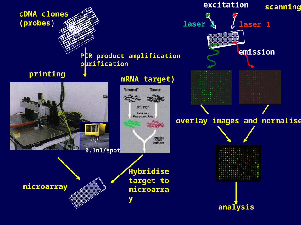
cDNA clones(probes)

PCR product amplificationpurification

printing

microarray

Hybridise target to microarray

mRNA target)

excitation

laser 1laser 2

emission

scanning

analysis

0.1nl/spot

overlay images and normalise

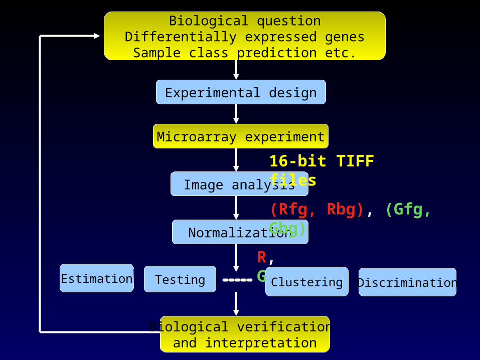
Biological questionDifferentially expressed genesSample class prediction etc.

Testing

Biological verification and interpretation

Microarray experiment

Estimation

Experimental design

Image analysis

Normalization

Clustering Discrimination

R, G

16-bit TIFF files

(Rfg, Rbg), (Gfg, Gbg)

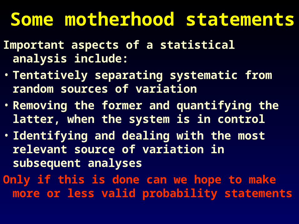
Some motherhood statementsSome motherhood statementsImportant aspects of a statistical analysis

include:• Tentatively separating systematic from

random sources of variation• Removing the former and quantifying the

latter, when the system is in control• Identifying and dealing with the most relevant

source of variation in subsequent analyses

Only if this is done can we hope to make more or less valid probability statements

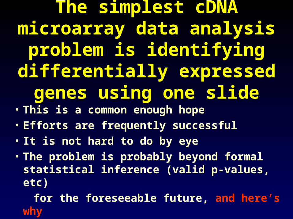
The simplest cDNA microarray The simplest cDNA microarray data analysis problem is data analysis problem is identifying differentially identifying differentially

expressed genes using one slideexpressed genes using one slide

• This is a common enough hope

• Efforts are frequently successful

• It is not hard to do by eye

• The problem is probably beyond formal statistical inference (valid p-values, etc)

for the foreseeable future, and here’s why

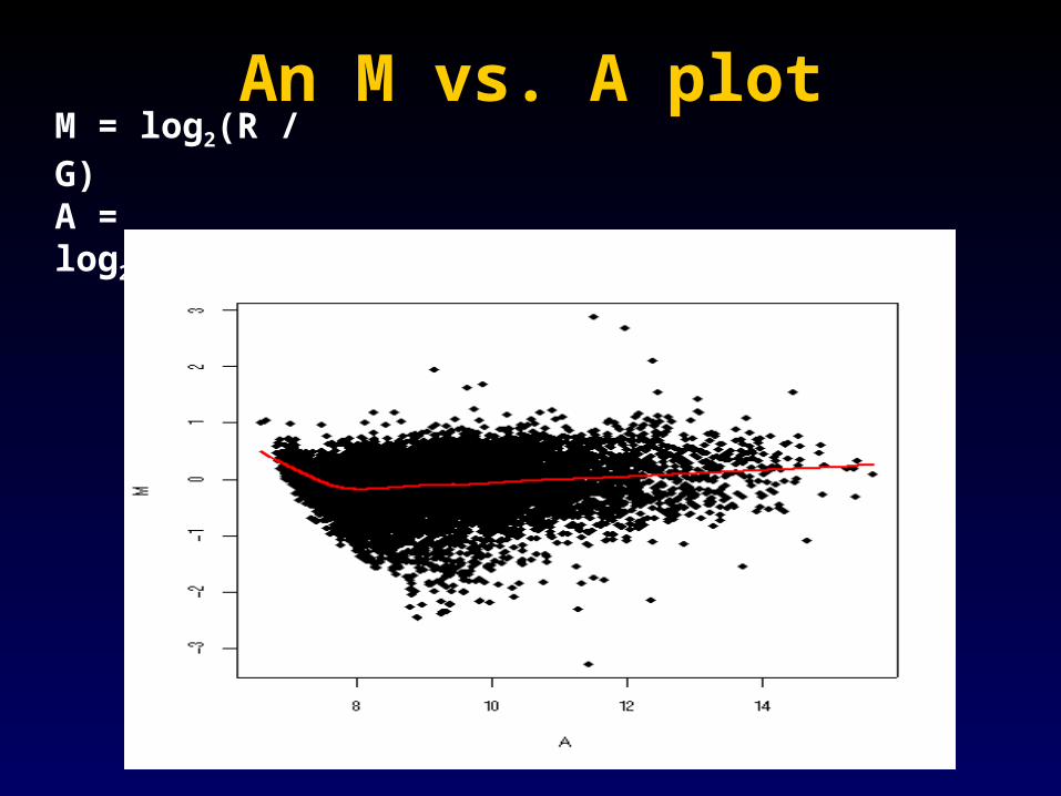
An M vs. A plotAn M vs. A plotM = log2(R / G)A = log2(R*G) / 2

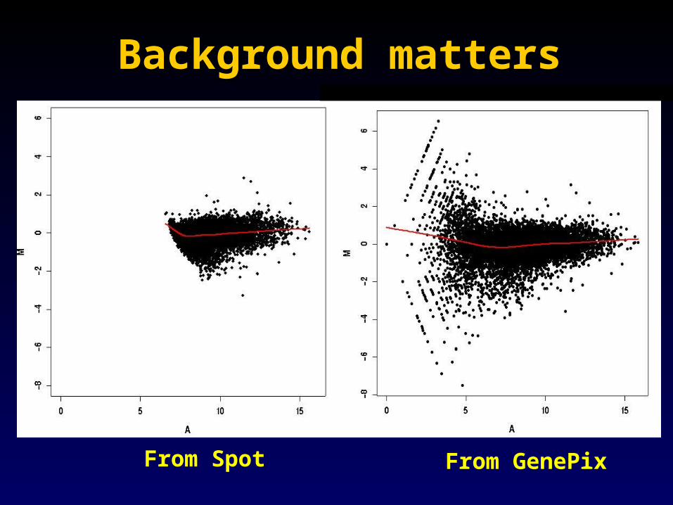
Background mattersBackground matters

From Spot From GenePix

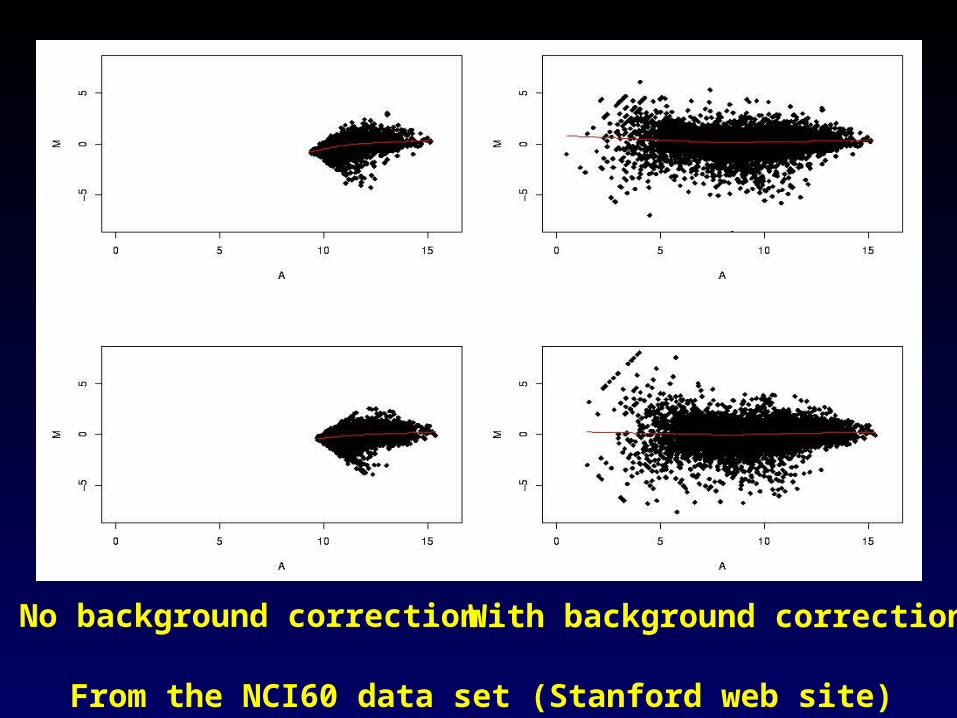
From the NCI60 data set (Stanford web site)

No background correction With background correction

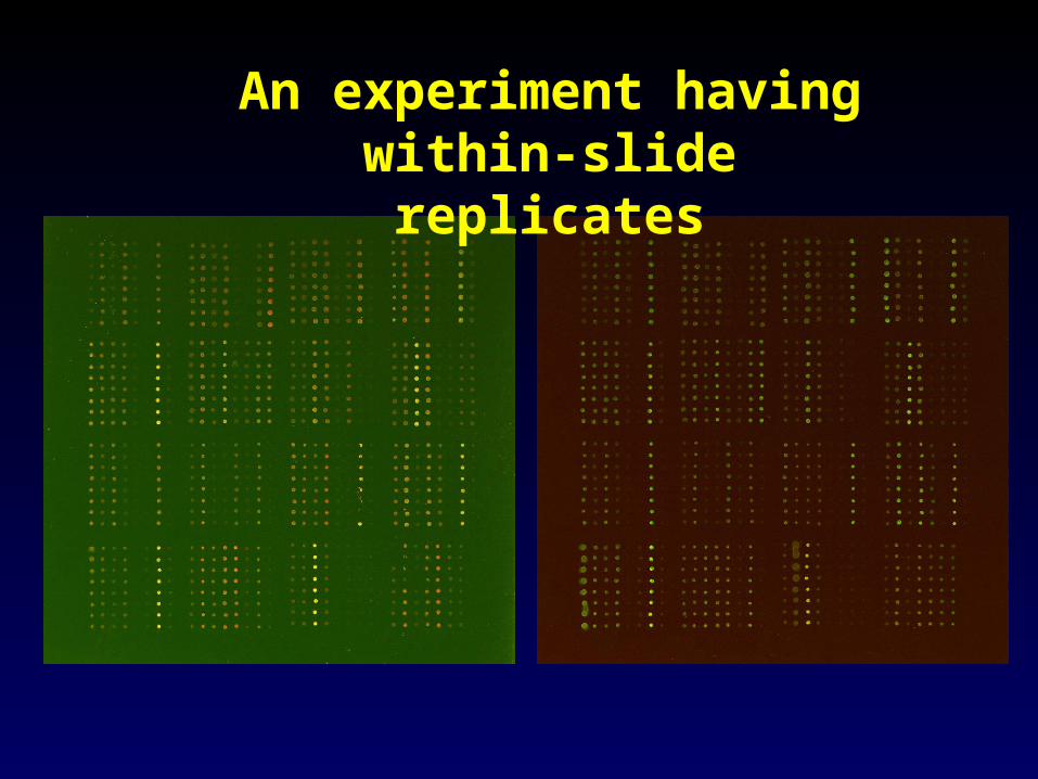
An experiment having within-slide replicates

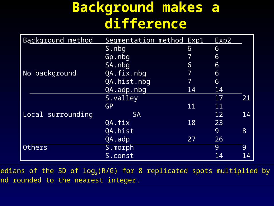
Background makes a differenceBackground makes a difference

Background method Segmentation method Exp1 Exp2S.nbg 6 6Gp.nbg 7 6SA.nbg 6 6

No background QA.fix.nbg 7 6QA.hist.nbg 7 6QA.adp.nbg 14 14S.valley 17 21GP 11 11

Local surrounding SA 12 14QA.fix 18 23QA.hist 9 8QA.adp 27 26

Others S.morph 9 9S.const 14 14

Medians of the SD of log2(R/G) for 8 replicated spots multiplied by 100and rounded to the nearest integer.

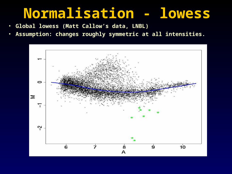
Normalisation - lowessNormalisation - lowess• Global lowess (Matt Callow’s data, LNBL)• Assumption: changes roughly symmetric at all intensities.

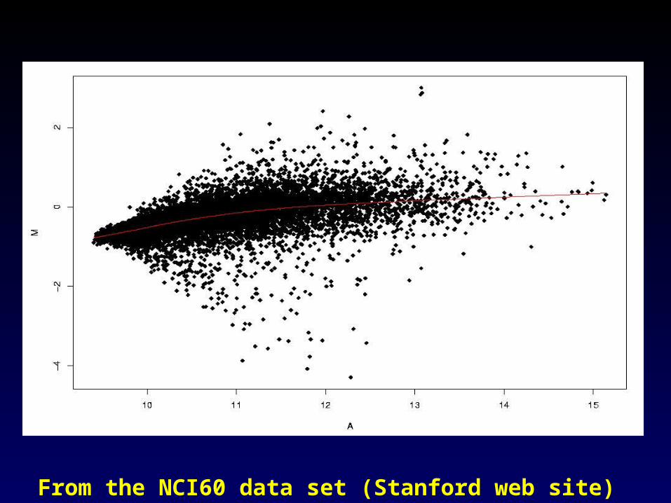
From the NCI60 data set (Stanford web site)

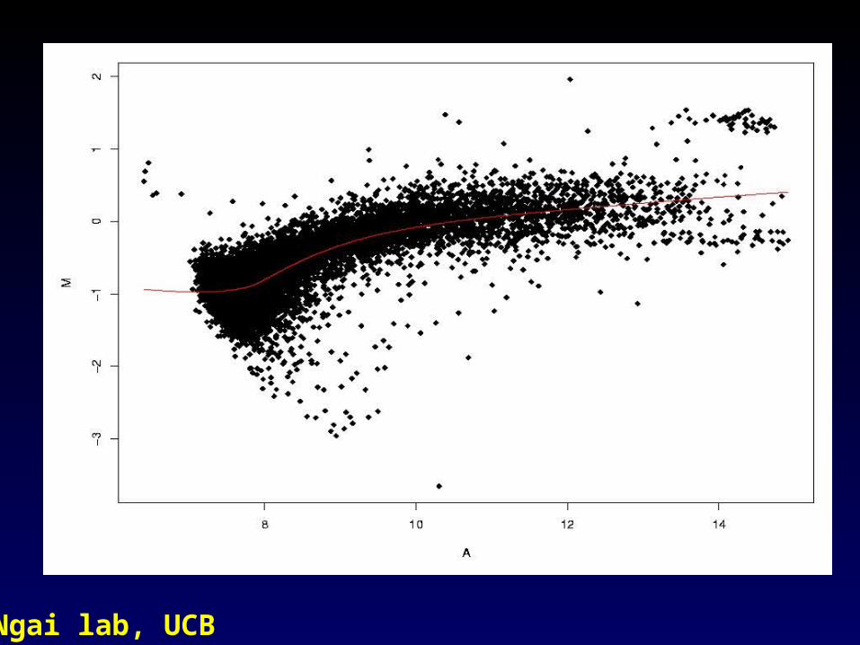
Ngai lab, UCB

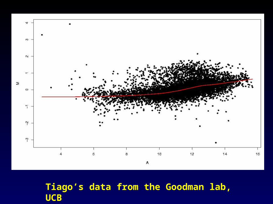
Tiago’s data from the Goodman lab, UCB

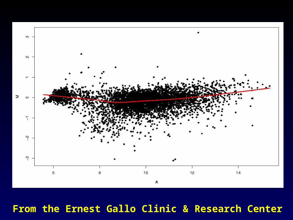
From the Ernest Gallo Clinic & Research Center

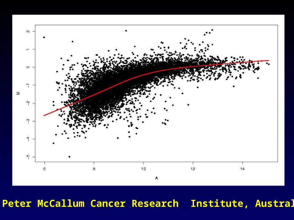
From Peter McCallum Cancer Research Institute, Australia

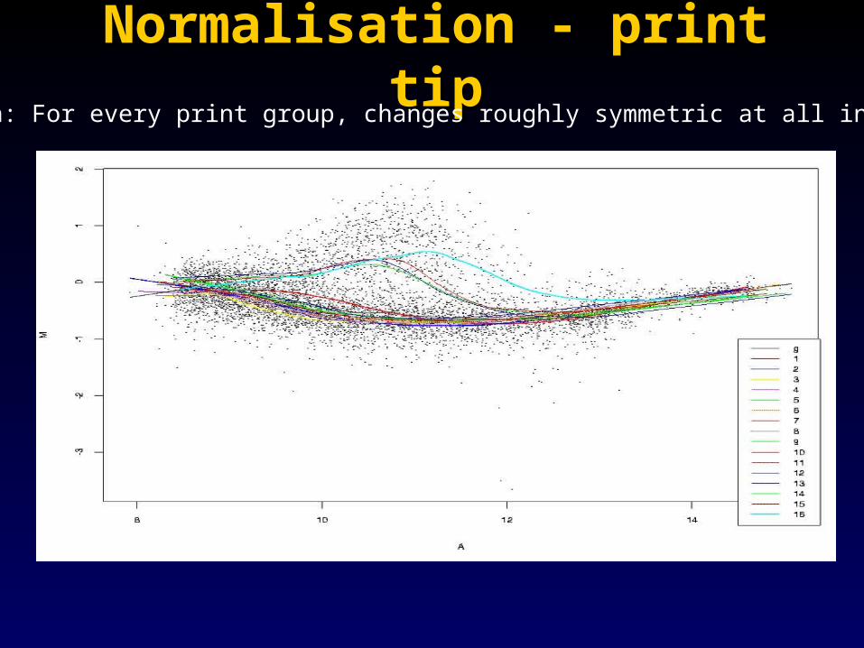
Normalisation - print tipNormalisation - print tipAssumption: For every print group, changes roughly symmetric at all intensities.

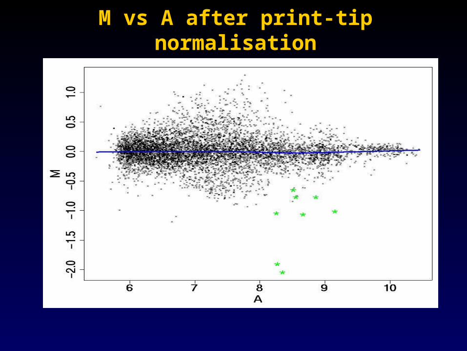
M vs A after print-tip normalisationM vs A after print-tip normalisation

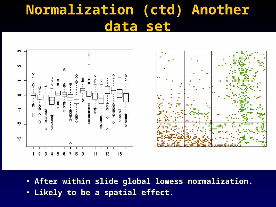
Normalization (ctd) Another data setNormalization (ctd) Another data set

• After within slide global lowess normalization.• Likely to be a spatial effect.

Print-tip groups

Lo

g-r

ati o

s

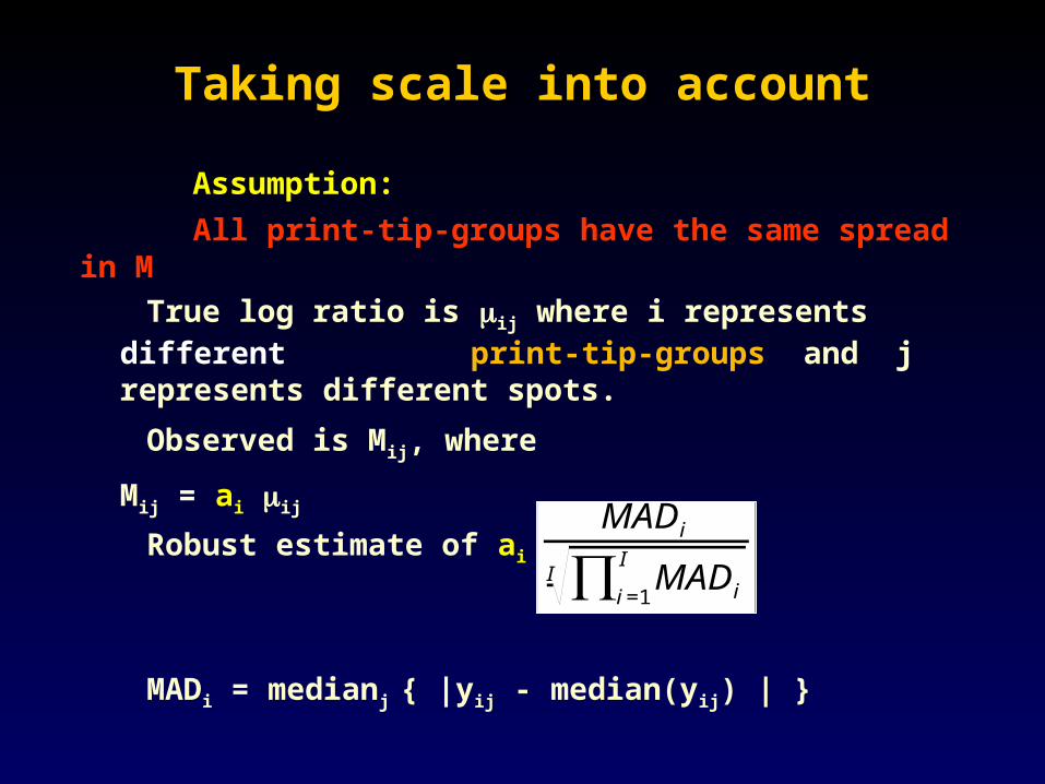
Assumption:

All print-tip-groups have the same spread in M

True log ratio is ij where i represents different print-tip-groups and j represents different spots.

Observed is Mij, where

Mij = ai ij

Robust estimate of ai is

MADi = medianj { |yij - median(yij) | }

Taking scale into accountTaking scale into account

MADi

MADii=1

I∏I

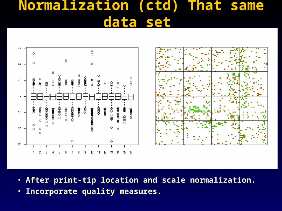
Normalization (ctd) That same data setNormalization (ctd) That same data set

• After print-tip location and scale normalization.• Incorporate quality measures.

Lo

g-r

ati o

s

Print-tip groups

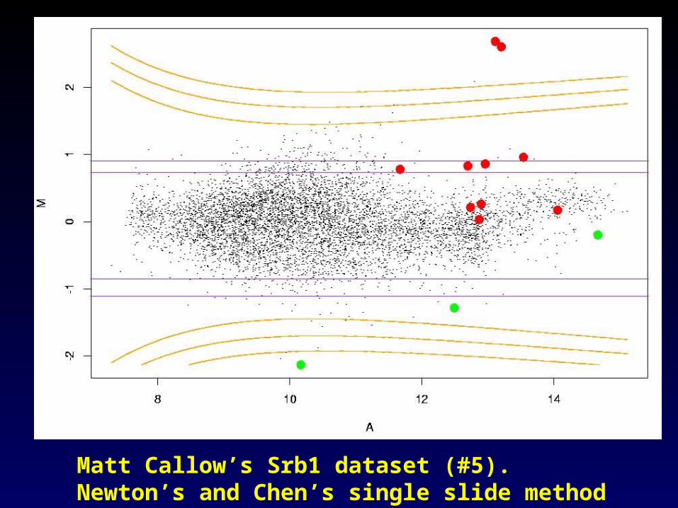
Matt Callow’s Srb1 dataset (#5). Newton’s and Chen’s single slide method

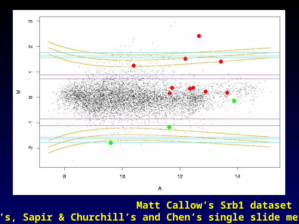
Matt Callow’s Srb1 dataset (#8). Newton’s, Sapir & Churchill’s and Chen’s single slide method

10

100

1000

10000

100000

10 100 1000 10000 100000

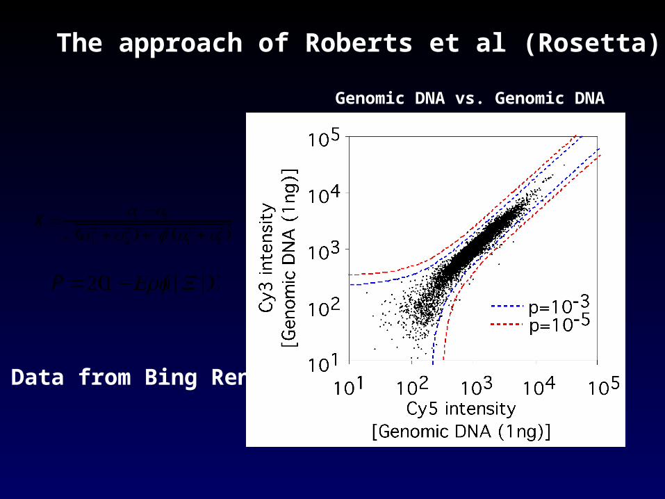
Genomic DNA vs. Genomic DNA

The approach of Roberts et al (Rosetta)

X =a1 −a2

(σ12 +σ2

2 ) + f2 (a12 +a2

2 )

P=2(1−Erf(|X |))

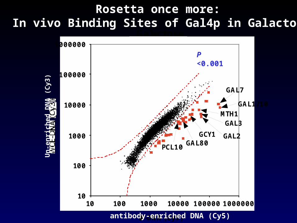
Data from Bing Ren

The second simplest cDNA microarray The second simplest cDNA microarray data analysis problem is identifying data analysis problem is identifying differentially expressed genes using differentially expressed genes using

replicated slidesreplicated slides

There are a number of different aspects:• First, between-slide normalization; then• What should we look at: averages, SDs t-

statistics, other summaries?• How should we look at them?• Can we make valid probability statements?

A report on work in progress

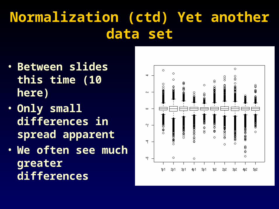
Normalization (ctd) Yet another data set

• Between slides this time (10 here)

• Only small differences in spread apparent

• We often see much greater differences

Slides

Lo

g-r

ati o

s

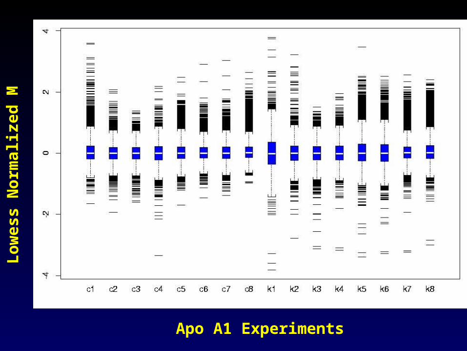
Apo A1 Experiments

Lo

wes

s N

orm

aliz

ed M

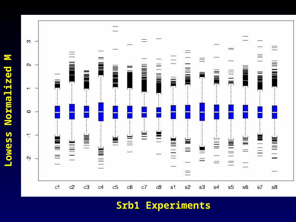
Srb1 Experiments

Lo

wes

s N

orm

aliz

ed M

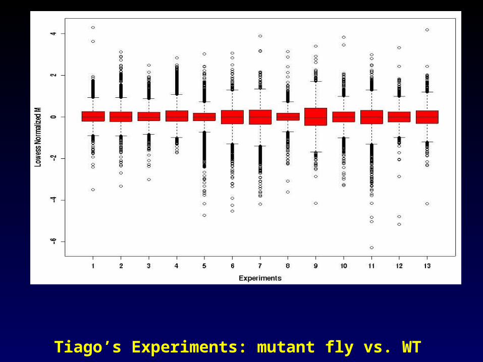
Tiago’s Experiments: mutant fly vs. WT

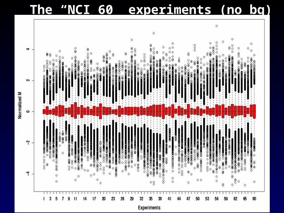
The “NCI 60” experiments (no bg)

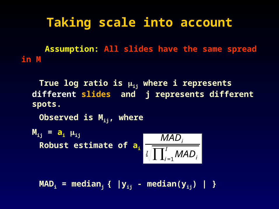
Assumption: All slides have the same spread in M

True log ratio is ij where i represents different slides and j represents different spots.

Observed is Mij, where

Mij = ai ij

Robust estimate of ai is

MADi = medianj { |yij - median(yij) | }

Taking scale into accountTaking scale into account

MADi

MADii=1

I∏I

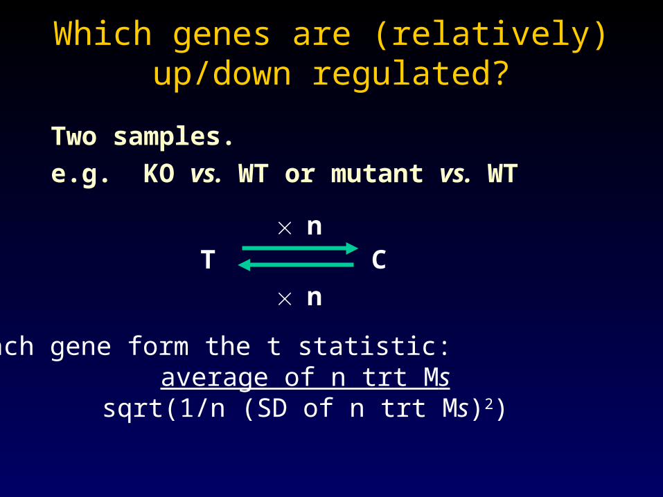
Which genes are (relatively) up/down Which genes are (relatively) up/down regulated?regulated?

Two samples.

e.g. KO vs. WT or mutant vs. WT

T C n

For each gene form the t statistic: average of n trt Ms

sqrt(1/n (SD of n trt Ms)2)

n

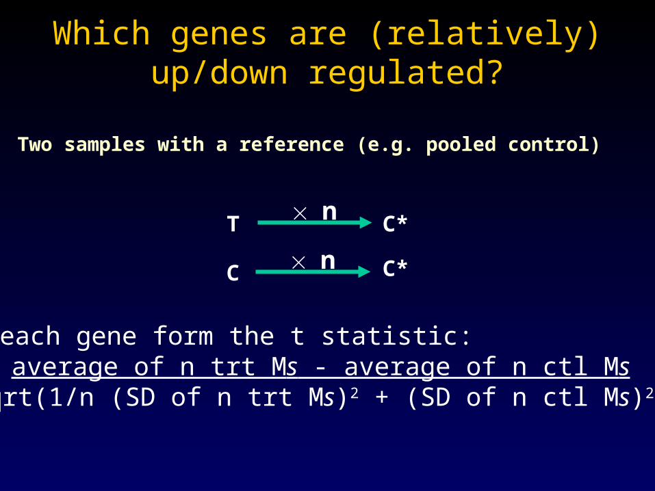
Which genes are (relatively) up/down Which genes are (relatively) up/down regulated?regulated?

Two samples with a reference (e.g. pooled control)

T C* n

• For each gene form the t statistic: average of n trt Ms - average of n ctl Ms

sqrt(1/n (SD of n trt Ms)2 + (SD of n ctl Ms)2)

C C* n

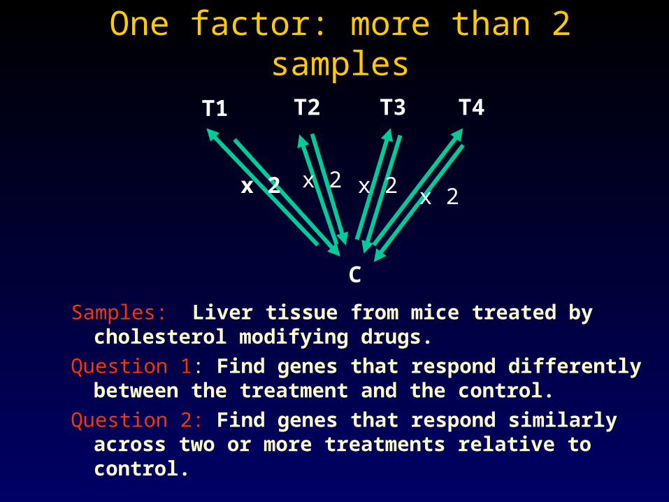
One factor: more than 2 samplesOne factor: more than 2 samples

Samples: Liver tissue from mice treated by cholesterol modifying drugs.

Question 1: Find genes that respond differently between the treatment and the control.

Question 2: Find genes that respond similarly across two or more treatments relative to control.

T1

C

T2 T3 T4

x 2x 2x 2 x 2

One factor: more than 2 samplesOne factor: more than 2 samples

Samples: tissues from different regions of the mouse olfactory bulb.

Question 1: differences between different regions.

Question 2: identify genes with a pre-specified patterns across regions.

T3 T4

T2

T6T1

T5

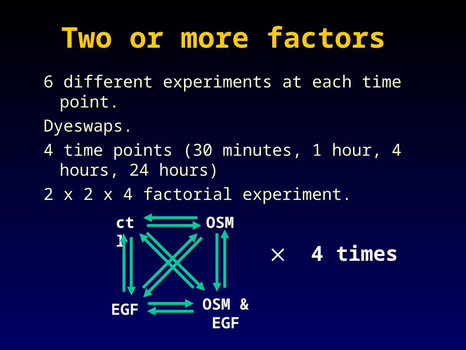
Two or more factorsTwo or more factors

6 different experiments at each time point.

Dyeswaps.

4 time points (30 minutes, 1 hour, 4 hours, 24 hours)

2 x 2 x 4 factorial experiment.

ctl OSM

EGF OSM & EGF

4 times

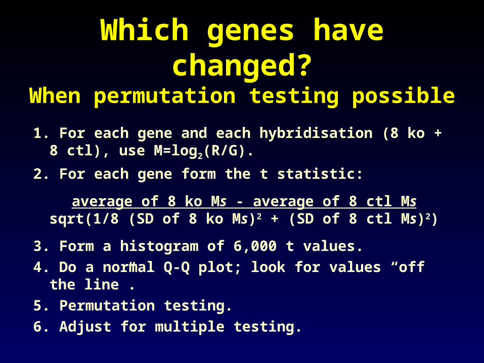
Which genes have changed?Which genes have changed?When permutation testing possibleWhen permutation testing possible

1. For each gene and each hybridisation (8 ko + 8 ctl), use M=log2(R/G).

2. For each gene form the t statistic:

average of 8 ko Ms - average of 8 ctl Mssqrt(1/8 (SD of 8 ko Ms)2 + (SD of 8 ctl Ms)2)

3. Form a histogram of 6,000 t values.

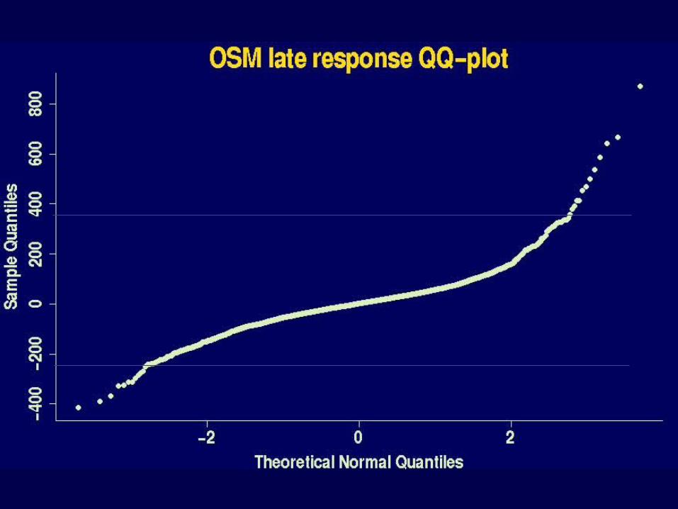
4. Do a normal Q-Q plot; look for values “off the line”.

5. Permutation testing.

6. Adjust for multiple testing.

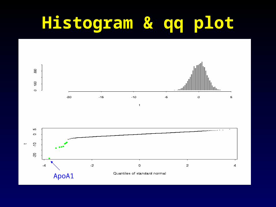
Histogram & qq plotHistogram & qq plot

ApoA1

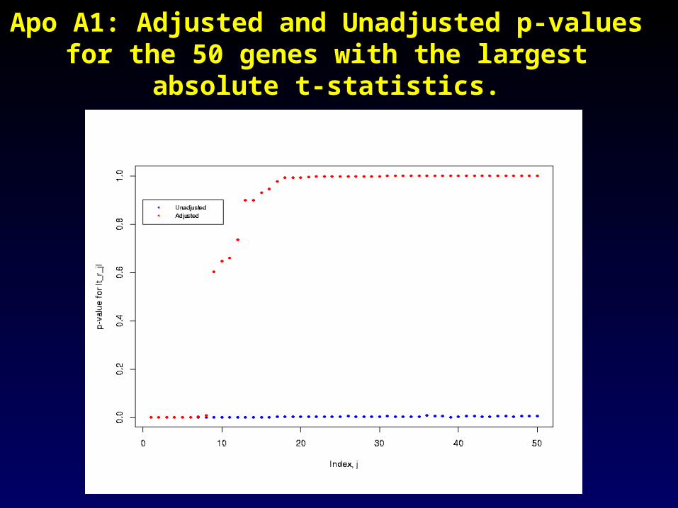
Apo A1: Adjusted and Unadjusted p-values for the Apo A1: Adjusted and Unadjusted p-values for the 50 genes with the largest absolute t-statistics.50 genes with the largest absolute t-statistics.

Which genes have changed?Which genes have changed?Permutation testing not possiblePermutation testing not possible

Our current approach is to use averages, SDs, t-statistics and a new statistic we call B, inspired by empirical Bayes.

We hope in due course to calibrate B and use that as our main tool.

We begin with the motivation, using data from a study in which each slide was replicated four times.

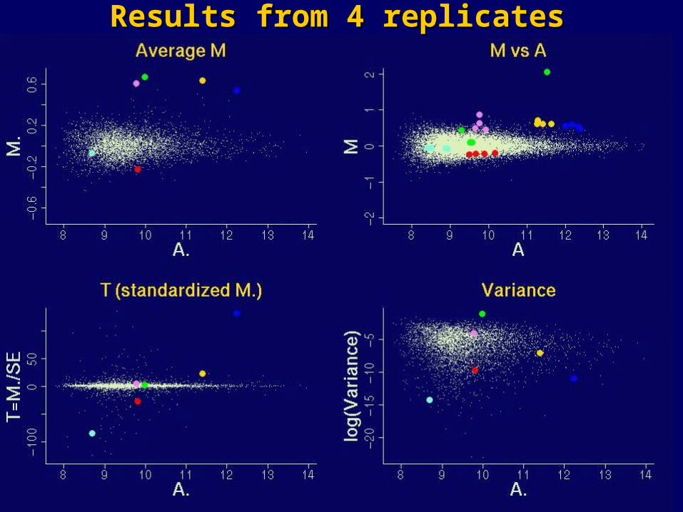
Results from 4 replicatesResults from 4 replicates

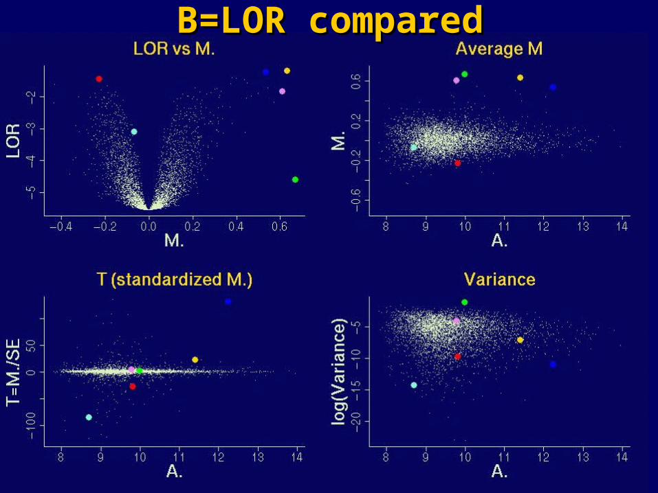
B=LOR comparedB=LOR compared

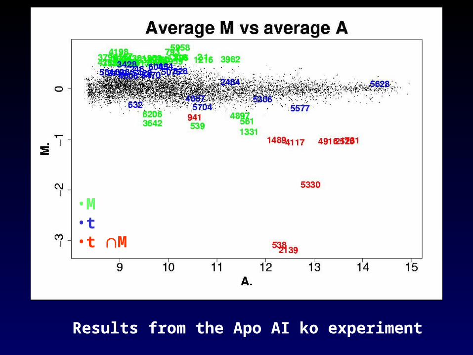
•M •t•t M

Results from the Apo AI ko experiment

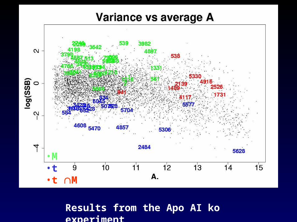
•M •t•t M

Results from the Apo AI ko experiment

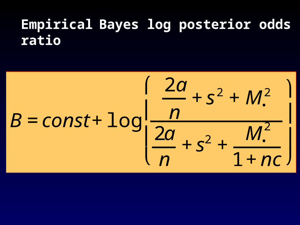
B=const+log

2an

+s2 +M•2

2an

+s2 +M•

2

1+nc

⎛

⎝

⎜ ⎜

⎞

⎠

⎟ ⎟

Empirical Bayes log posterior odds ratio

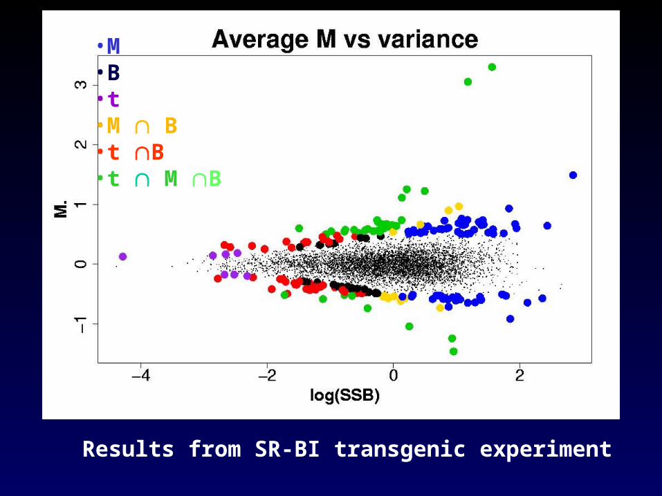
•M •B•t•M B•t B•t M B

Results from SR-BI transgenic experiment

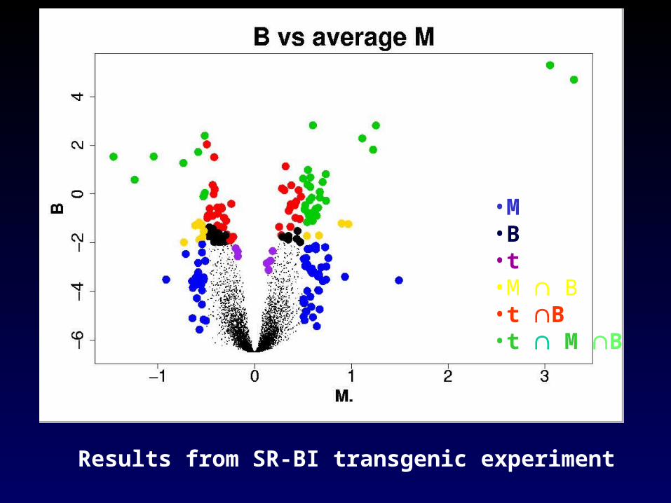
•M •B•t•M B•t B•t M B

Results from SR-BI transgenic experiment

Extensions include dealing withExtensions include dealing with

• Replicates within and between slides

• Several effects: use a linear model

• ANOVA: are the effects equal?

• Time series: selecting genes for trends

10

100

1000

10000

100000

1000000

10 100 1000 10000 100000 1000000

Galactose

PCL10GAL80

GAL1/10

GAL2

GAL3

GAL7

GCY1

MTH1

WCE-DNA (Cy3)

IP-DNA (Cy5)

Un

-en

rich

ed D

NA

(C

y3)

antibody-enriched DNA (Cy5)

Rosetta once more: In vivo Binding Sites of Gal4p in Galactose

P <0.001

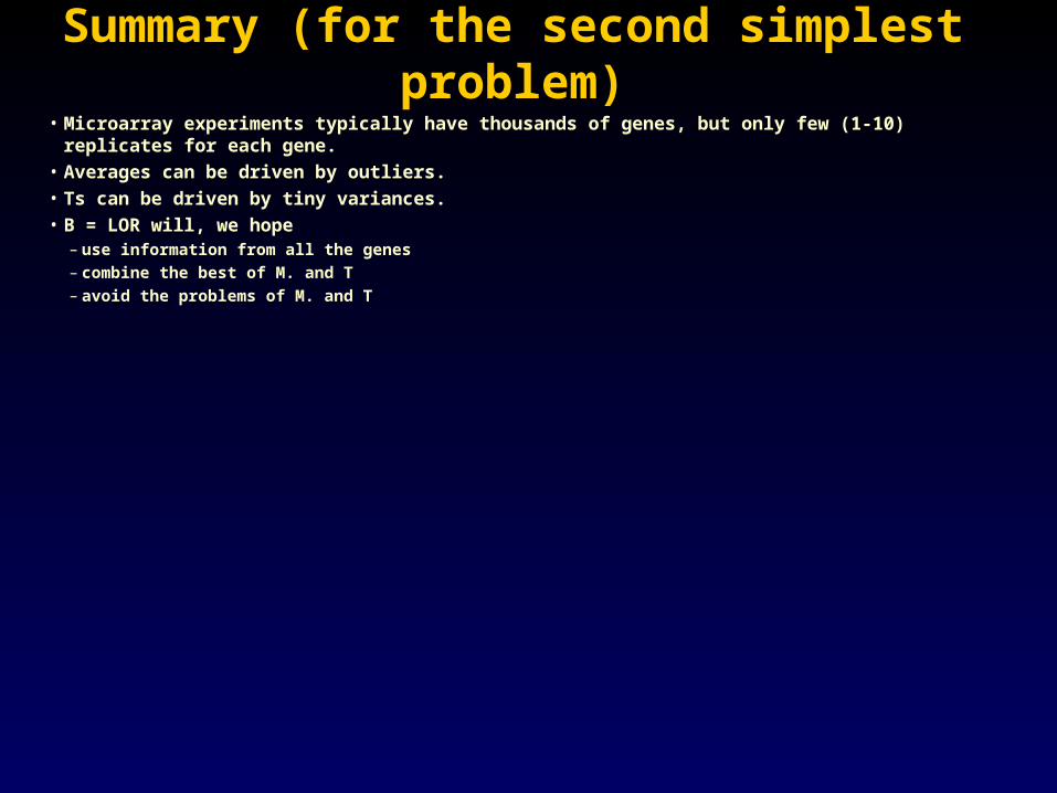
Summary (for the second simplest problem)Summary (for the second simplest problem)• Microarray experiments typically have thousands of genes, but only few (1-10) replicates for each gene.• Averages can be driven by outliers.• Ts can be driven by tiny variances.• B = LOR will, we hope

– use information from all the genes– combine the best of M. and T– avoid the problems of M. and T

AcknowledgmentsAcknowledgments

UCB/WEHIUCB/WEHI

Yee Hwa YangYee Hwa Yang

Sandrine DudoitSandrine Dudoit

Ingrid Lönnstedt

Natalie Thorne Natalie Thorne

David FreedmanDavid Freedman

CSIRO Image Analysis Group

Michael BuckleyMichael Buckley

Ryan Lagerstorm

Ngai lab, UCB

Goodman lab, UCB

Peter Mac CI, Melb.

Ernest Gallo CRC

Brown-Botstein lab

Matt Callow (LBNL)

Bing Ren (WI)Bing Ren (WI)

Some web sites:

Technical reports, talks, software etc.

http://www.stat.berkeley.edu/users/terry/zarray/Html/

Statistical software R “GNU’s S” http://lib.stat.cmu.edu/R/CRAN/

Packages within R environment:

-- Spot http://www.cmis.csiro.au/iap/spot.htm

-- SMA (statistics for microarray analysis) http://www.stat.berkeley.edu/users/terry/zarray/Software /smacode.html

OSM, EGF and breast cancerOSM, EGF and breast cancer• Oncostatin M (OSM)

• is a cytokine in the interleukin 6 (IL-6) family• inhibits proliferation of breast caner cells (and

other cancer cells) • increases the expression of EGRF mRNA

• Epidermial growth factor (EGF)• is a polypeptide growth factor• overcomes effects of several breast inhibitors• enhances the effect of OSM on breast cancer

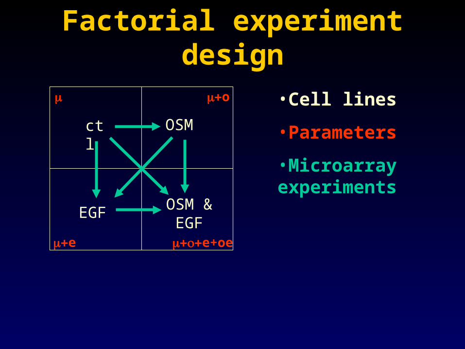
ctl OSM

EGF OSM & EGF

o

e e+oe

Factorial experiment designFactorial experiment design

•Cell lines

•Parameters

•Microarray experiments

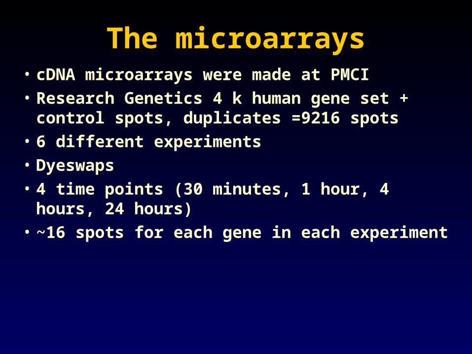
The microarraysThe microarrays• cDNA microarrays were made at PMCI• Research Genetics 4 k human gene set +

control spots, duplicates =9216 spots• 6 different experiments• Dyeswaps• 4 time points (30 minutes, 1 hour, 4 hours, 24

hours)• ~16 spots for each gene in each experiment

Back to the factorial designBack to the factorial design

ctl OSM

EGF OSM & EGF

o

e e+oe

•Different ways of estimating each effect

•Ex: 1 = ( + o) - ()

= o

2 - 5 = ( + o + e + oe) - ()

-(( + o + e + oe)-( + o))

=(o + e + oe) - (e + oe)

=o

3 + 6 =…=o

•How do we use all the information?

1

53

4

2 6

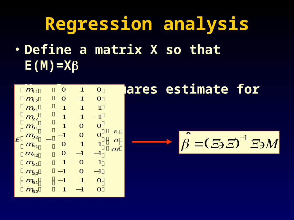
Regression analysisRegression analysis• Define a matrix X so that E(M)=X

• Use least squares estimate for o, e, oe

E

m11

m12

m21

m22

m31

m32

m41

m42

m51

m52

m61

m62

⎛

⎝

⎜ ⎜ ⎜ ⎜ ⎜ ⎜ ⎜ ⎜ ⎜ ⎜ ⎜ ⎜

⎞

⎠

⎟ ⎟ ⎟ ⎟ ⎟ ⎟ ⎟ ⎟ ⎟ ⎟ ⎟ ⎟

=

0 1 00 −1 01 1 1

−1 −1 −11 0 0

−1 0 00 1 10 −1 −11 0 1

−1 0 −1−1 1 01 −1 0

⎛

⎝

⎜ ⎜ ⎜ ⎜ ⎜ ⎜ ⎜ ⎜ ⎜ ⎜ ⎜ ⎜

⎞

⎠

⎟ ⎟ ⎟ ⎟ ⎟ ⎟ ⎟ ⎟ ⎟ ⎟ ⎟ ⎟

eooe

⎛

⎝

⎜ ⎜

⎞

⎠ ⎟ ⎟ ˆ = X' X( )−1X'M

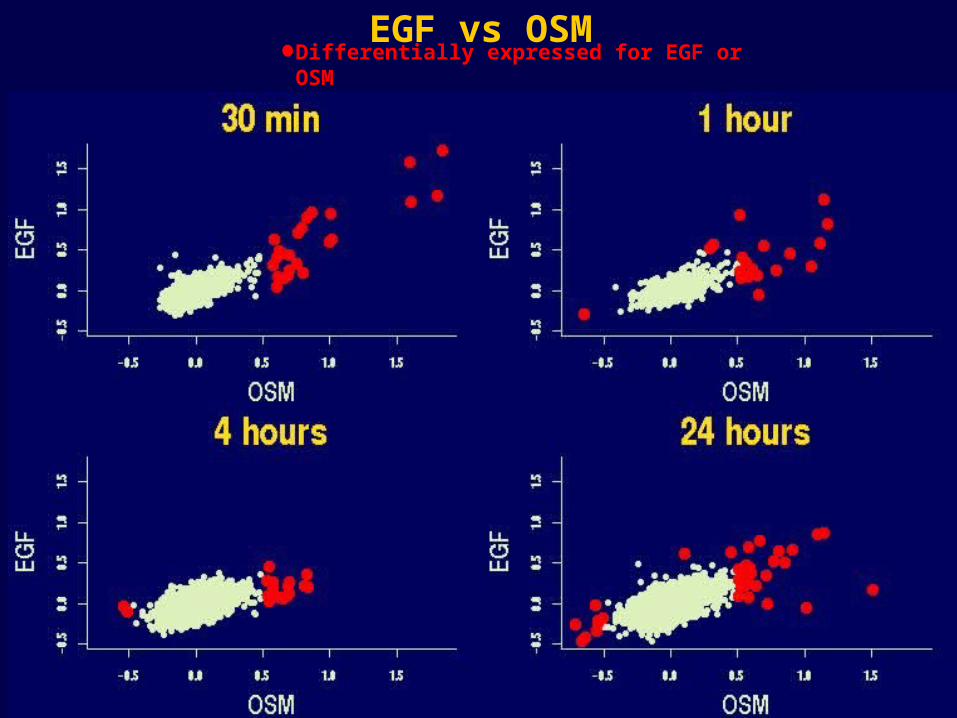
EGF vs OSMDifferentially expressed for EGF or OSM

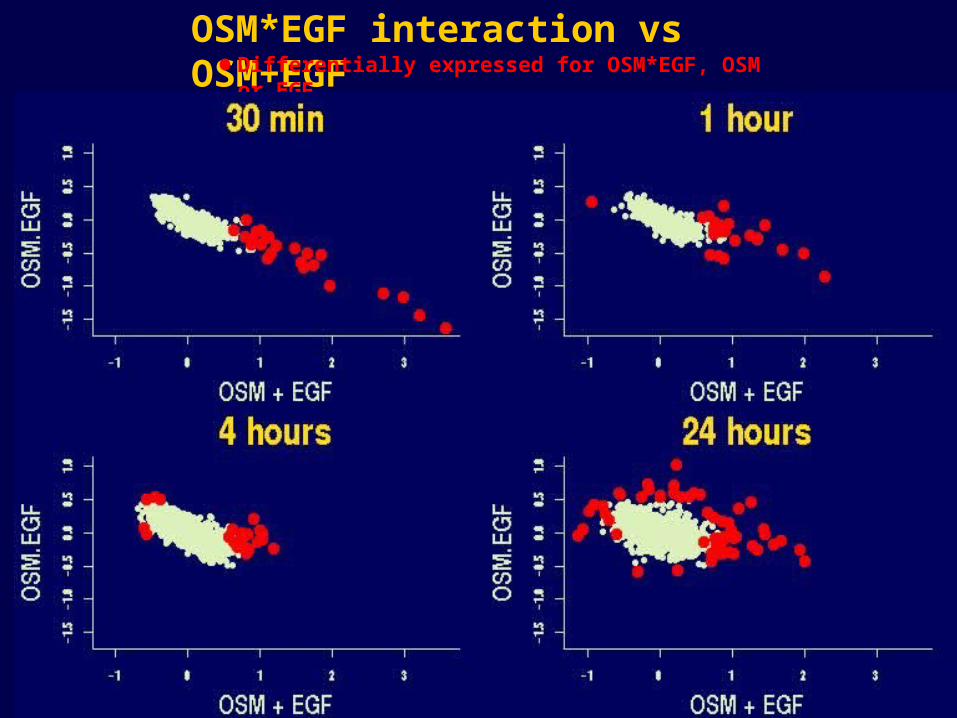
OSM*EGF interaction vs OSM+EGFDifferentially expressed for OSM*EGF, OSM or EGF

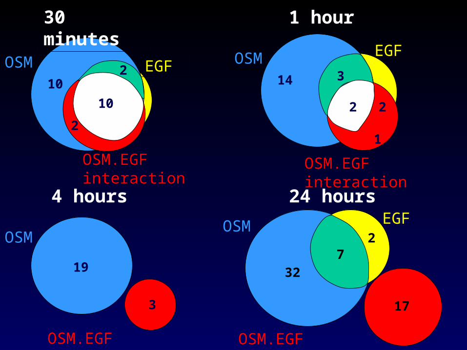
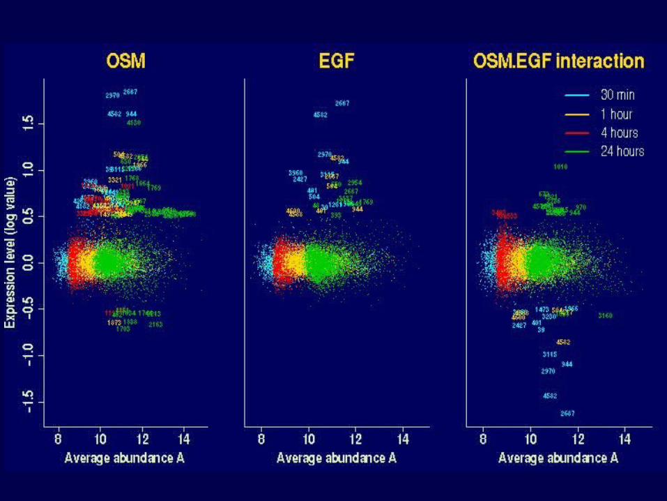
OSM.EGF interaction

OSM10

10

2

30 minutes

EGF

OSM.EGF interaction

OSM14

10

EGF

OSM.EGF interaction

2

2

3

2

1

OSM

19

3

1 hour

4 hours 24 hours

10

OSM

32

EGF

OSM.EGF interaction

7

17

2

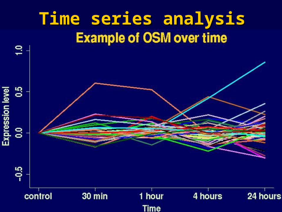
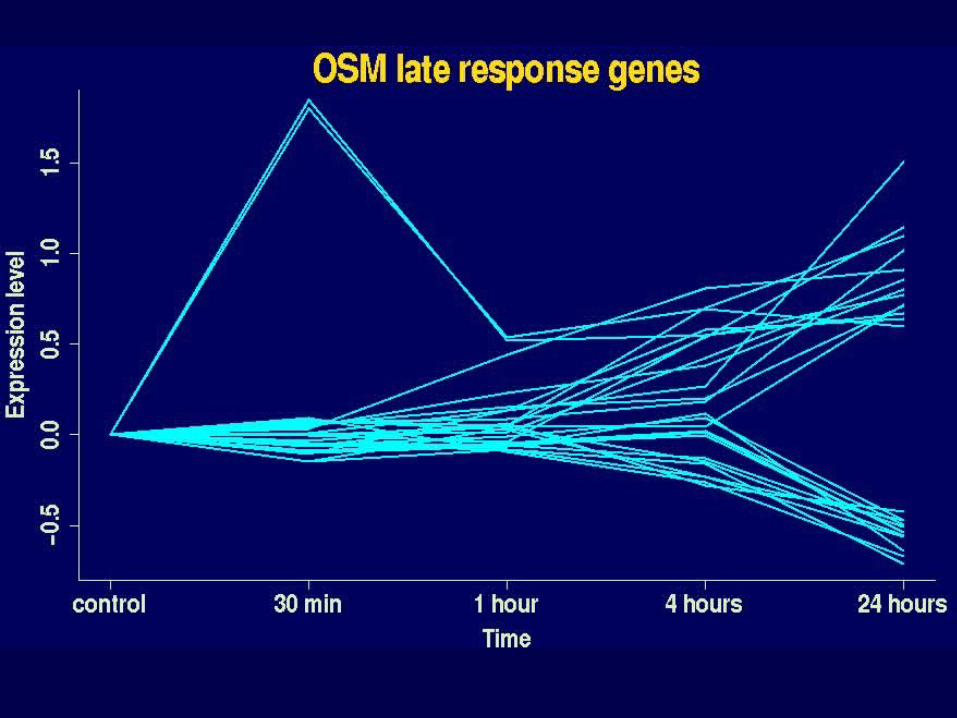
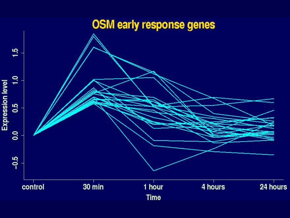
Time series analysisTime series analysis

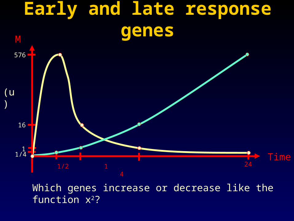
Early and late response genesEarly and late response genes

1/2 1 4 24Time

M

Which genes increase or decrease like the function x2?

1

16

576

1/4

(u)

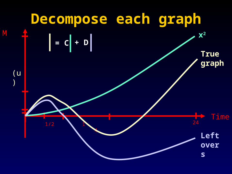
Decompose each graphDecompose each graph

1/2 1 4 24Time

True graph

x2

Left overs

= C + DM

(u)

Vector worldVector world• For each gene, we have a vector, y, of expression estimates at the

different time points

• Project the vector onto the space spanned by the vector u (the values of x2 at our time points).

• C is the scalar product

u

C

y

u

C

y

C =y • u=

y30y1y4y24

⎛

⎝

⎜ ⎜ ⎜

⎞

⎠

⎟ ⎟ ⎟•

1/ 4116576

⎛

⎝

⎜ ⎜ ⎜

⎞

⎠

⎟ ⎟ ⎟

10

OSMEGF

OSM.EGF interaction

1

Early response genes

8

OSM EGF

OSM.EGF interaction

3

Late response genes

11

2

1

17

25

19

6

1