The Signaling Petri Net-Based Simulator: A Non- …nakhleh/Papers/RuthsEtAl-PLoS08.pdf · Parametric Strategy for Characterizing the Dynamics of ... dynamics of signal flow through

The Signaling Petri Net-Based Simulator: A Non-Parametric Strategy for Characterizing the Dynamics ofCell-Specific Signaling NetworksDerek Ruths1*, Melissa Muller2, Jen-Te Tseng2, Luay Nakhleh1, Prahlad T. Ram2

1 Department of Computer Science, Rice University, Houston, Texas, United States of America, 2 Department of Systems Biology, University of Texas M. D. Anderson

Cancer Center, Houston, Texas, United States of America

Abstract

Reconstructing cellular signaling networks and understanding how they work are major endeavors in cell biology. The scaleand complexity of these networks, however, render their analysis using experimental biology approaches alone verychallenging. As a result, computational methods have been developed and combined with experimental biologyapproaches, producing powerful tools for the analysis of these networks. These computational methods mostly fall oneither end of a spectrum of model parameterization. On one end is a class of structural network analysis methods; thesetypically use the network connectivity alone to generate hypotheses about global properties. On the other end is a class ofdynamic network analysis methods; these use, in addition to the connectivity, kinetic parameters of the biochemicalreactions to predict the network’s dynamic behavior. These predictions provide detailed insights into the properties thatdetermine aspects of the network’s structure and behavior. However, the difficulty of obtaining numerical values of kineticparameters is widely recognized to limit the applicability of this latter class of methods. Several researchers have observedthat the connectivity of a network alone can provide significant insights into its dynamics. Motivated by this fundamentalobservation, we present the signaling Petri net, a non-parametric model of cellular signaling networks, and the signalingPetri net-based simulator, a Petri net execution strategy for characterizing the dynamics of signal flow through a signalingnetwork using token distribution and sampling. The result is a very fast method, which can analyze large-scale networks,and provide insights into the trends of molecules’ activity-levels in response to an external stimulus, based solely on thenetwork’s connectivity. We have implemented the signaling Petri net-based simulator in the PathwayOracle toolkit, which ispublicly available at http://bioinfo.cs.rice.edu/pathwayoracle. Using this method, we studied a MAPK1,2 and AKT signalingnetwork downstream from EGFR in two breast tumor cell lines. We analyzed, both experimentally and computationally, theactivity level of several molecules in response to a targeted manipulation of TSC2 and mTOR-Raptor. The results from ourmethod agreed with experimental results in greater than 90% of the cases considered, and in those where they did notagree, our approach provided valuable insights into discrepancies between known network connectivities and experimentalobservations.

Citation: Ruths D, Muller M, Tseng J-T, Nakhleh L, Ram PT (2008) The Signaling Petri Net-Based Simulator: A Non-Parametric Strategy for Characterizing theDynamics of Cell-Specific Signaling Networks. PLoS Comput Biol 4(2): e1000005. doi:10.1371/journal.pcbi.1000005

Editor: Satoru Miyano, The University of Tokyo, Japan

Received September 18, 2007; Accepted January 18, 2008; Published February 29, 2008

Copyright: � 2008 Ruths et al. This is an open-access article distributed under the terms of the Creative Commons Attribution License, which permitsunrestricted use, distribution, and reproduction in any medium, provided the original author and source are credited.

Funding: DR and LN were supported in part by a Seed Grant awarded to LN from the Gulf Coast Center for Computational Cancer Research, funded by John andAnn Doerr Fund for Computational Biomedicine. J-TT was supported in part by a training fellowship from the Pharmacoinformatics Training Program of the KeckCenter of the Gulf Coast Consortia (NIH grant 5 T90 DK070109-03), and MM and PTR were supported in part by Department of Defense grant BC044268 to PTR.

Competing Interests: The authors have declared that no competing interests exist.

* E-mail: [email protected]

Introduction

Signaling networks are complex, interdependent cascades of

signals that process extracellular stimuli, received at the plasma

membrane of a cell, and funnel them to the nucleus, where they

enter the gene regulatory system. These signaling networks

underlie how cells communicate with one another, and how they

make decisions about their phenotypic changes, such as division,

differentiation, and death. Further, malfunction of these networks

may alter phenotypic changes that cells are supposed to undergo

under normal conditions, and potentially lead to devastating

consequences on the organism. For example, altered cellular

signaling networks can give rise to the oncogenic properties of

cancer cells [1,2], increase a person’s susceptibility to heart disease

[3], and have been shown to be responsible for many other

devastating diseases such as congenital abnormalities, metabolic

disorders and immunological abnormalities [1,4].

In light of the crucial role signaling networks play in the

proper functioning of cells and biological systems as a whole, and

given the grave consequences their alterations may have on the

behavior of cells, elucidating the connections in the networks,

and understanding how they operate, are two central questions

in cell biology. However, unlike the ‘‘pathway view’’ of signaling

as linear cascades, signaling networks are highly interconnected,

involve cross-talk among several pathways, and contain feedback

and feed-forward loops [5]. Figure 1 illustrates this issue in a

network of signaling cascades, which is stimulated by EGF and

contains several players in cancer pathways. For example,

multiple paths lead from EGFR to mTOR-Raptor, resulting in

feed-forward loops. Some of these paths activate mTOR-Raptor,

PLoS Computational Biology | www.ploscompbiol.org 1 2008 | Volume 4 | Issue 2 | e1000005

while others inhibit it. Further, the network contains two

feedback loops, one from p70S6K to EGFR and another from

MAPK1,2 to EGFR.

These and other complexities make it very difficult to analyze

signaling networks by experimental biology approaches alone. As a

result, computational methods have been developed and com-

bined with experimental biology approaches, producing powerful

tools for the analysis of these networks [6]. These computational

methods produce hypotheses that guide the experimental design,

leading to more informative experiments, while experimental

results help refine the computational models, resulting in more

accurate predictive tools.

In a recent survey, Papin et al. classified existing computational

methods into two categories: structural and dynamic network analysis

[6]. Structural network analysis is mainly based on the network’s

connectivity, which is typically readily available from numerous

public signaling network databases (e.g., [7–9]), and makes

inferences about global network properties as well as individual

protein functions. This category can be further refined into two

sub-categories, both of which are solely based on connectivity

information, yet differ in the type of answers they provide. For

example, the methods described in [10–13] infer ‘‘static’’

properties of the network, such as numbers of paths, reachability

results, etc. In a series of papers, Palsson and co-workers [6,14–16]

introduced extreme pathway analysis techniques, which are more

appropriate for metabolic networks, yet have been applied to

signaling networks to characterize various properties of networks,

such as redundancy and cross-talk. Similar analyses have also been

Figure 1. The Model Signaling Network. A MAPK1,2 and AKT network downstream from EGFR, which we assembled from various sources, and usedfor the case study analysis in this work. An edge from u to v ending with an arrow indicates an activating reaction, while an edge ending with a plungerindicates an inhibiting reaction. With the exception of TSC2, all nodes have self-inhibitory edges, which were added to model the external cellularmachinery that regulates the concentration of the active form of the proteins [36–43]. Colors were selected to enhance readability of the network.doi:10.1371/journal.pcbi.1000005.g001

Author Summary

Many cellular behaviors including growth, differentiation,and movement are influenced by external stimuli. Suchexternal stimuli are obtained, processed, and carried to thenucleus by the signaling network—a dense network ofcellular biochemical reactions. Beyond being interestingfor their role in directing cellular behavior, deleteriouschanges in a cell’s signaling network can alter a cell’sresponses to external stimuli, giving rise to devastatingdiseases such as cancer. As a result, building accuratemathematical and computational models of cellularsignaling networks is a major endeavor in biology. Thescale and complexity of these networks render themdifficult to analyze by experimental techniques alone,which has led to the development of computationalanalysis methods. In this paper, we present a novelcomputational simulation technique that can providequalitatively accurate predictions of the behavior of acellular signaling network without requiring detailedknowledge of the signaling network’s parameters. Ourapproach makes use of recent discoveries that networkstructure alone can determine many aspects of anetwork’s dynamics. When compared against experi-mental results, our method correctly predicted 90% ofthe cases considered. In those where it did not agree, ourapproach provided valuable insights into discrepanciesbetween known network structure and experimentalobservations.

Signaling Petri Net-Based Simulator


formalized and conducted using the principles of S- and T-

invariants in Petri Nets (e.g., [17–20]).

Methods for dynamic network analysis use, in addition to the

network connectivity, the kinetic parameters of the biochemical

reactions. The goal of these methods is to model the actual kinetics of

the network and obtain through simulation the actual quantities of

proteins involved in signal transduction. One of the most widely used

techniques in this category is systems of ordinary differential

equations (ODEs) (e.g., [21–25]). Within such a system, each

reaction is modeled by a series of equations connecting reactant

concentrations to product concentrations through differential

relationships involving reaction rate constants. Given the difficulty

of obtaining the numerical values of kinetic parameters [19,26] and

standardization of the parameters and models [27], the applicability

of these methods is limited in practice to small-scale networks [6,28].

Petri Nets have also been used for simulating the dynamics of

signaling networks [29–31]. While such approaches somewhat relax

the necessity for biologically exact kinetic parameters, current Petri

Net-based approaches still require the selection of weights and/or

probability distributions for individual interactions in the model. As a

result, selecting the values for Petri Net parameters presents

challenges similar to those encountered in ODE modeling.

Structural network analysis assumes mainly connectivity infor-

mation about the model, and provides insights into global, static

properties of the network. Dynamic analysis in general assumes

numerical values of the kinetic parameters, and provides predictions

of network dynamics by quantifying the change in concentration and

activity-level (the concentration of the active form of a given protein)

of the individual proteins and complexes in the network. To obtain a

more detailed analysis one must either solve parameter optimization

problems for a large number of molecules and interactions or

conversely experimentally derive these values.

Given the difficulty of obtaining numerical values of kinetic

parameters [19,26] and the implications this has on the

applicability of dynamic analysis methods [6], it is imperative to

develop innovative approaches that combine the attractive low

requirements of structural network analysis techniques with the

detailed answers provided by dynamic analysis techniques—

specifically the response of individual proteins to signals which

travel through the network.

Several recent efforts in this direction have produced encour-

aging results. An approach using a boolean network simulation

method, based on work in the area of gene regulatory networks,

successfully used only signaling network connectivity information

to predict the speed of signal transduction through a stomata

signaling network [32]. The use of piecewise linear systems of

ODEs have also had success in analyzing some of the dynamics of

gene regulatory and signaling networks without using exact kinetic

parameters (e.g., [33–35]). The obstacle to extending the method

in [32] to model individual protein responses to signal transduc-

tion is the boolean model used to discretize the signal as it

propagates. In a boolean model, the signal is either present or

absent at each node in the network. Such two-state models of

signal transduction simplify the underlying biochemistry to the

point where it is difficult to model changes in protein

concentration more precisely than present or absent. Modeling

such gradients of concentration changes and the effects of those

changes may be important to predicting individual protein

responses, motivating our effort to devise more fine-grained ways

to model and simulate the dynamics of signaling networks. The

challenges to using linear-piecewise ODEs to model a signaling

network center around the issue of identifying all the ODEs

required to model the underlying network as well as scalability

issues involved in simulating large systems of ODEs.

In this paper, we extend the synchronized Petri net model and

firing policy such that the resulting framework models cellular

signaling processes. We call this extension the signaling Petri net

(SPN). By coupling this with a novel strategy for Petri net

execution and sampling, we obtain a method capable of

characterizing some dynamics of signaling networks while using

only connectivity information about these networks.

To validate our method, we studied the MAPK1,2 and AKT

network shown in Figure 1 in two breast cancer cell lines. This

network was chosen because the EGFR receptor and its

downstream signaling network play a very important role in

development, differentiation, and oncogenic transformation. Two

very important signaling molecules within the cell are MAPK and

AKT, both of which can be activated by EGFR, and contains

several potential regulatory paths between them. We constructed a

model network of EGF regulation of MAPK and AKT which

includes several feedback and feed-forward loops all of which were

constructed based on experimental findings from different

laboratories around the world [36–43]. We analyzed, both

experimentally and computationally, the change in activity-level

of several proteins in response to targeted manipulation of TSC2

and mTOR-Raptor. Using the model network, the predictions

from our method agreed with experimental results in over 90% of

the cases, and in those where they did not agree, our method

correctly identified discrepancies that could be traced back to

incompleteness in the network connectivity model.

Materials and Methods

Our approach combines elements of the boolean network

simulator in [18] with a synchronized Petri net model [44]. In [18],

Li et al. present a non-parametric approach that accurately predicts

the speed of signal propagation through a network. However, as their

method assumes a binary model of activation—every protein is either

active (true) or inactive (false)—modeling a range of activity-levels is

difficult. Petri nets, while able to model concentrations using tokens,

require parameters describing the kinetic characteristics of the

network, which are typically difficult to obtain.

Our method models signal flow as the pattern of token

accumulation and dissipation within places (proteins) over time

in the Petri net. Transitions in the network represent directed

protein interactions; each transition models the effect of a source

protein on a target protein. Through transition firings, the source

can influence the number of tokens assigned to the target, called

the token-count, modeling the way that signals propagate through

protein interactions in cellular signaling networks.

In order to overcome the issue of modeling reaction rates in the

network, signaling dynamics are simulated by executing the

signaling Petri net (SPN) for a set number of steps (called a run)

multiple times, each time beginning at the same initial marking.

For each run, the individual signaling rates are simulated via

generation of random orders of transition firings (interaction

occurrences). When the results of a large enough number of runs

are averaged together, we find that the series of token-counts

correlate with experimentally measured changes in the activity-

levels of individual proteins in the underlying signaling network. In

essence, the tokenized activity-levels computed by our method

should be taken as abstract quantities whose changes over time

correlate to changes that occur in the amounts of active proteins

present in the cell. It is worth noting that some of the most widely

used experimental techniques for protein quantification—western

blots and microarrays—also yield results that are treated as

indications, but not exact measurements, of protein activity-levels

within the cell. Thus in some respects, the predictions returned by



our SPN-based simulator can be interpreted like the results of a

western blot or microarray experiment looking at changes relative

to ‘‘control’’.

The key insight behind our approach is the assumption that,

while all network parameters determine the actual signal

propagation to some extent, the network connectivity is the most

significant single determinant. While this is clearly a gross

simplification, several researchers have observed that the connec-

tivity of a biological network dictates, to a great extent, the

network’s dynamics [18,45–47]. Some have conjectured that

biological network connectivities have evolved to have a stabilizing

effect on the overall network behavior, making the network more

resilient to local fluctuations in other network parameters such as

reaction rates and protein binding affinities [45,47]. Here we

present the signaling Petri net (SPN) model and the signaling Petri

net-based simulator whose designs collectively utilize this assump-

tion and couple it with a Petri net tokenization scheme that

quantifies the changes in protein activity-levels that occur as

signals propagate through the network. In the following sections,

we describe the synchronized Petri net, how we extended it to

create the signaling Petri net, and a novel strategy for executing

the signaling Petri net to simulate signaling network dynamics.

Petri NetsA Petri net is a graph that consists of two types of nodes, places,

and transitions [44]. Edges in the graph, called arcs, are directed and

connect places to transitions or transitions to places. Thus, the

Petri net is a bipartite graph. Formally, a Petri net is a 4-tuple

Q = ÆP,T,I,Oæ where

P = {p1,p2,…,pm} is the set of places,

T = {t1,t2,…,tn} is the set of transitions,

I = {i1,i2,…,ik} is the set of input arcs where for all (u,v)MI, uMP

and vMT, and

O = {o1,o2,…,ol} is the set of output arcs where for all (u,v)MI, uMT

and vMP.

In order to simulate a dynamic process, a number of tokens is

assigned to each place in order to indicate the presence of some

quantitative property. This assignment of tokens to places encodes

the state of the system and is called a marking, denoted m. A

marked Petri net, R = ÆQ,m0æ, is a Petri net with a marking m0, called

the initial marking. For the remainder of this paper, the term Petri

net (PN) refers to a marked Petri net.

Changes in the state of the system are simulated by executing the

Petri net—evaluating the effect of transitions on the marking of the

network. These changes in marking are induced by sequential firing

one or more transitions. When a transition fires, it removes a token

from each place connected to it by input arcs and adds a token to

each place connected to it by output arcs. The number of tokens

removed from inputs and added to outputs can be specified by

weighting the input arcs. However, as our extension does not use

this weighting property, we do not consider this very common PN

formulation here.

A transition can only fire when it is enabled, meaning that each of

its input places has at least one token in the current marking. If a

transition t, when fired on a marking m1, produces marking m2,

then we write m1|tæm2.

This notation can be extended to represent the effect of firing a

series of transitions. A firing sequence, s= (t1,t2,…,tj) is a sequence of

transitions. The sequence’s cumulative effect on the system’s state

is denoted m0|sæmf where m0 is the initial marking and mf is the

marking produced by the firing of the sequence of transitions in

the order specified in s. In this paper, we write msg to indicate the

marking produced by the first g transitions in s. Therefore, in the

above example, ms0~m0 and ms

sj j~mf .

For a more complete introduction to types of Petri nets and

their properties, we refer the reader to [44].

Synchronized Petri nets. Synchronized Petri nets model

systems in which the firing of a transition is triggered by a specific

event that occurs in the environment. The marked Petri net is

extended to include a set of these events and a mapping function

that assigns an event to each transition. When transition t’s

assigned event occurs, transition t is fired. Formally, a

synchronized Petri net is a 3-tuple ÆR,E,Syncæ, where [44]:

R is a marked Petri net,

E = {e1,e2,…,es} is a set of events, and

Sync:TRE<{e} maps each transition in the Petri net to an

event. Event e is the always occurring event. Any transition associated

with e is always immediately fired upon becoming enabled.

When executing a synchronized Petri net, transition t is fired

when its associated event e = Sync(t) occurs. The order in which

events are generated depends upon the environment which

generates them. Just as in the marked Petri net, when a transition

fires, it removes one token from each place connected by input

arcs and gives one token to each place connected by output arcs.

As will be discussed in the next sections, we extend the

synchronized Petri net paradigm to model the dynamics of a

signaling network. To our knowledge, ours is the first use of the

synchronized Petri net to model biochemical systems. In principle

it is well suited to signaling networks since places represent

proteins, tokens represent concentrations, and transitions represent

directed protein interactions. A model of signaling event

occurrence can be used to generate events and fire transitions,

providing a way of simulating the signaling network’s behavior.

These and other design details will be discussed in the next section.

The Signaling Petri Net-Based SimulatorA high-level sketch of our simulator is given is Figure 2. Details

and rationale for specific design decisions will be discussed in

subsequent sections.

During the simulation, the input signaling Petri net is executed

multiple times on a firing sequence constructed by the signaling

event generator. The signaling event generator imposes an

ordering on transition firing such that it creates a two-time scale

simulation. The smaller time scale is discretized as the firing of a

single transition. This unit is referred to as the firing time scale.

Firing steps are nested within a larger time scale, called time blocks,

in which each transition is fired exactly once. Thus, there are |T|

firings per block. Since the simulation is run for the specified

number of time blocks, B, there are B|T| firing steps in the

simulation.

The time structure for an example simulation is illustrated in

Figure 3. This dual-time approach is necessitated by the rate

parameter sampling strategy we employ. Since the rate parameters

are not known, our method executes many simulation runs (Step 2 in

Figure 2) in order to sample the space of possible rate parameters.

The markings returned by these runs are then averaged (Step 3 in

Figure 2). The only requirement placed on the different rate

parameter values is that all events occur within the same larger time

frame—the time block. Therefore, within every time block all edges

are evaluated once, though not necessarily in the same order.

This idea of evaluating random event orderings within a two-

time scale system has appeared before in the domain of

transcriptional networks [48]. In that study, Chaves et al.

employed a two-time scale formulation of network updates similar

in concept to the one we describe here. In their work, they

assumed a boolean model of regulation and characterized the



effect of different relative rates of transcription within the same

network on the final steady state reached. In contrast, our method

is designed to operate on tokenized models of signaling networks

with the ultimate intent of predicting the activity-level changes of

proteins in the underlying signaling network over time.

In the next sections, we discuss in greater detail the core design

decisions underlying our method: the signaling Petri net, transition

firing, signaling network event generator, constructing the initial

marking for the model, and sampling signaling rates. We then

discuss how our strategy can be used to predict the outcome of

perturbation experiments.

The Signaling Petri NetThe goal of our method is to predict the signal flow through a

cell-specific network under specific experimental conditions. As a

result, the signaling Petri net model must characterize the

connectivity of the signaling network, the connectivity-level

network properties that are unique to the cell type and

experimental conditions under which the network is being studied,

and the signaling processes of activation and inhibition.

The signaling Petri net is a synchronized Petri net with: 1) a

specific way of modeling activating and inhibiting interactions

using places, transitions, and arcs; 2) a one-to-one correspondence

between events and transitions such that every transition is

associated with a unique event; 3) modified rules regarding how

many tokens are moved in response to a transition firing; and 4) a

signaling network event generator.

Places correspond to the activated forms of signaling proteins.

The number of tokens assigned to place p in marking ms, ms(p),

abstractly represents the amount of active protein p present in that

network state. Signaling interactions are modeled using transitions

and their connected input and output arcs. Each transition, t, is

associated with a unique signaling event, e, such that when e

occurs, transition t fires. Figure 4 shows the equivalent signaling

Petri net for a signaling network.

Formally, a signaling Petri net is a 3-tuple S = ÆR,E,Syncæ, where:

R is a marked Petri net,

E is a set of signaling events such that |E| = |T| and there is no

always occurring event, and

Sync:TRE is a one-to-one mapping which assigns each

transition a unique signaling event.

The initial marking of a signaling Petri net, m0, represents the

state of rest from which the network is starting and being simulated.

Proteins whose concentrations are known to be high can be given a

large number of tokens, and those whose concentrations are known

to be low can be assigned few or zero tokens. Attention to the initial

marking is central to modeling cell-specific networks. In many cell

lines, specific proteins are known to contain mutations that render

them perpetually active or inactive [49]. Furthermore, experimental

studies frequently involve the targeted manipulation of various

proteins within the network. Both of these phenomena induce state

changes in certain proteins at various time points that must be

modeled. The way in which these are modeled will be discussed

when the simulator design is explained.

Transition FiringWhen a signaling interaction ARB (A activates B) or AxB (A

inhibits B) occurs, it has the effect of changing the state of the system

by modifying the activity-level of A and/or B. Thus, in the SPN

used to model this network, the associated transition, t, will fire at

Figure 2. A High-Level Outline of the Procedure for Simulating a Signaling Network. The input to the procedure is a signaling Petri net, S,the number of time units to simulate the network for, B, and the number of runs for which to repeat the simulation, r. The random generation ofevent ordering is employed to simulate the stochasticity in reaction rates and the differing times of signal arrivals.doi:10.1371/journal.pcbi.1000005.g002

Figure 3. The Effects of Reaction Rates on Signal Propagation. (A) By changing the speed of signaling edge 3, the value of D at the end of asingle simulation step can be reversed. If edge 3 is slower than the cascade BRCxD, then D will be active. If edge 3 is faster than the cascade, then Dwill be inactive. (B) An example of how the simulator might evaluate the individual edges during a run. In each time block, every edge is evaluatedonce. Each edge evaluation corresponds to one time step. Note that the order of the edge evaluation is shuffled during each time block in order tosample the space of possible relative signaling rates.doi:10.1371/journal.pcbi.1000005.g003



time t and produce marking mt+1 from mt. The way in which

mt+1 is computed from mt depends on the set of input and output

arcs attached to the transition as well as the number of tokens

moved by the transition.

The combination of input and output arcs connected to a

transition is determined exclusively by the type of interaction and

the transition firing model. However, different topologies,

combinations of input and output arcs, are needed to model the

different biochemical processes that mediate protein-protein

interactions in a signaling network. Here we examine four of the

most common biochemical processes, identify the corresponding

topological motifs, and ultimately devise a modeling policy best

suited for non-parametric simulation of signal flow.

In post-translational modification (PTM), a protein mediates the

addition or removal of a phospho group at a specific phosphor-

ylation site on another protein. In GTP/ATP binding, a protein

triggers the exchange of GDP (ADP) from GTP (ATP) on another

protein. In a recruitment process, a protein mediates the relocaliza-

tion of another protein to a different part of the cell. Finally, in a

complexing process, a protein binds to another protein to create a

complex, which can then participate in other reactions. In the first

two processes, the mediating protein usually acts as an enzyme

that participates in the reaction but is not consumed by the

reaction. In the latter two processes, the participating protein often

becomes unavailable to other reactions, transiently while the

protein recruitment is taking place and for longer durations when

complexing occurs. To model these two cases, we identified the

two different token-passing policies implemented by the different

topological motifs depicted in Figure 5.

Token consumption. In this policy, uPv consumes tokens in u

in order to generate new tokens for v. In order to model this, pu is

connected to transition t1 through an arc and pv is connected to t1through an output arc. When t1 fires, some number of tokens in pu

are moved into pv. Similarly, uxv consumes tokens in u in order to

consume tokens in v. This is modeled by connecting pu to t2 with an

input arc and pv to t2 with an input arc. When t2 fires, some number

of tokens are removed from both pu and pv. This policy models a

recruitment or complexing event in which u binds to another

molecule, thereby creating a molecule of type v. A molecule of type u has

been consumed in order to generate or deactivate a molecule of type v.

Token conservation. In this policy, uPv generates new

tokens for v while conserving those in u. In order to model this, pu

is connected to transition t3 through a read arc. Node pv is

connected to t3 through an output arc. When t3 fires, some

number of tokens in pu is read (but not removed) and copied into

pv. Similarly, uxv consumes tokens in v while conserving those in

u. This is modeled by connecting pu to t4 with a read arc and pv to

t4 with an input arc. When t4 fires, some number of tokens in pu

are read and removed from pv. Enzymes will often behave in this

way: inducing a change in a molecule (v) without themselves

undergoing any change. A molecule of u has induced a change in a

different molecule of type v without itself changing state.

Ideally, for each interaction in the network, the associated

transition could be embedded in the topology corresponding to the

interaction’s underlying biochemical mechanism. However, connec-

tivity-level knowledge of the network does not provide this

information for each interaction. In the absence of these details,

we use one token-passing policy for all interactions in the network.

We implemented and tested both the consuming and conserving

policies and found that token conservation provides significantly

more accurate results when compared to experimentally derived

data. This is not surprising, as post-translational modification and

GTP/ATP binding events are responsible for many activation state

changes in signaling networks [1,50–52]. It is worth noting that our

approach does not restrict the net structure to token conserving

topologies. Thus, it is possible to use the token consumption

topologies where such processes are known to occur. However, as

our focus in this paper is designing a purely non-parametric

simulation method, we consider the use of information regarding the

biological mechanism of signaling as a potential way to further

improve the accuracy of our method’s predictions and identify this as

a direction for future work.

Figure 4. An Example Signaling Network and Its Corresponding Petri Net. An example signaling network (A) and its corresponding Petri net(B). Each signaling protein in the network, A, B, and C, are designated as places pA, pB, and pC. Signaling interactions become a transition node and itsinput and output arcs. Note that the connectivity for an activating edge differs from that of an inhibitory edge.doi:10.1371/journal.pcbi.1000005.g004



The transition topologies, as described above, do not designate

how the number of tokens added to or removed from pv is

determined. However, we know that in biochemical signaling

networks concentration has an effect on the strength of a

signaling event [53–55]. Specifically, the higher u’s concentra-

tion, the stronger its effect on v—the more tokens that pu has,

the more tokens of pv should be affected (generated or

consumed).

However, because of the stochastic nature of the underlying

biochemistry, it would be inaccurate to assume that all active u

molecules will always participate in an interaction with v. In order

to accommodate this observation, when transition t fires, we

randomly select the number of pu’s tokens to be involved in the

subsequent evaluation of the transition, which we call a signaling

event. Note that, according to our choice of topology, pu can always

be identified as the node connected to the transition by a read arc.

In this paper, we assume a uniform distribution for selecting the

number of tokens involved in a given signaling event, but

acknowledge that other distributions may be more appropriate

under certain circumstances and identify this as a topic deserving

further consideration.

Let ms(x) denote the number of tokens in node x at time s. For an

interaction (u,v), under the token conservation policy detailed

above, u’s token-count remains unchanged after the firing of t,

whereas v’s token-count is updated based on the following

formula:

ms vð Þ~ms{1 vð Þzrandom 0,ms{1 uð Þð Þ if u activates v

max 0,ms{1 uð Þ{random 0,ms{1(u)ð Þf g if u inhibits v

�,

where random(p,q) is a random integer drawn from a uniform

distribution over the range [p,q].

If we employ the policy of token passing with consumption, then

after ms(v) has been computed based on the formula above, ms(u) is

updated as:

ms uð Þ~ms{1 uð Þ{ min ms{1 uð Þ, ms vð Þ{ms{1 vð Þj jf g:

Signaling Network Event GeneratorThe SPN topology and transition token-number selection policy

alone do not specify the speed with which individual signaling

interactions occur. However, such rates must be accounted for

when simulating a signaling network. ODEs characteristically

model such details as reaction rate constants; parameterized Petri

nets specify these in a variety of ways including transition firing

rates and firing probabilities [17,30]. In synchronized Petri nets,

the environment controls the generation of events. Thus, the

signaling network event generator is responsible for controlling the

timing and ordering of signaling events. However, as our objective

is a non-parametric simulation method, our approach must either

estimate these parameters or operate without explicit knowledge of

them.

Estimating reaction rates using only connectivity is currently

beyond the predictive or inferential capabilities of computers.

While there has been some work in the area of predicting reaction

rates, all results of which we are aware require knowledge about

the mechanism of signaling (e.g., [56]). As a result, without

enriching the SPN model, it is doubtful that rate parameters can

be accurately estimated.

For this reason, the signaling network event generator operates

without explicit knowledge of the rate parameters. To compensate

for this ‘‘missing’’ knowledge, we make use of an observation of

signaling networks discussed earlier: a network’s connectivity

determines its dynamics. Several studies have found that the

connectivity of biochemical networks desensitizes them to small

fluctuations in the kinetic biochemical parameters [45–47].

Understood within the context of evolution – a stochastic process

that tweaks signaling network parameters across generations – this

is a highly desirable property as it ensures that an offspring

remains viable despite fluctuations in the exact tuning of its cellular

machinery. If this property holds, then small fluctuations in the

rate parameters should have a marginal effect on the overall

propagation of signal through the network. We can consider these

small effects to be noise obscuring the underlying dynamics of the

network connectivity. By taking many samples of the network

dynamics under a variety of reaction rate assignments and then

averaging these dynamics, we simultaneously reduce the noise

Figure 5. The Topological Motifs for Differing Signaling Processes. (A) The token consumption motifs for complexing and recruitment.Transition t1 encodes activation of v by the binding or consumption of u. Transition t2 encodes deactivation of v by the binding or consumption of u.In both cases, the number of tokens of pu decreases immediately after transitions t1 and t2 fire. (B) The token conserving motifs for PTM and GTP/ATPbinding. Transition t3 encodes enzymatic activation of v by u. Transition t4 encodes enzymatic inhibition of v by u. In both cases, the number oftokens of pu remains unchanged immediately after transitions t3 and t4 fire.doi:10.1371/journal.pcbi.1000005.g005



introduced by any one rate assignment and strengthen the

underlying dynamic characteristics of the network’s connectivity.

However, since reaction rate constants can vary by several

orders of magnitude—from 10210 to 103, the task of correctly

selecting parameters close to the true parameters is non-trivial. In

fact, without having some estimate of the actual rate parameters, it

is unclear as to how to measure closeness at all. Clearly, these are

among the issues that make parameter estimation so difficult for

ODE and Petri net approaches. Since our comparisons will be

relative and not absolute, we take a relative approach to modeling

rate parameters. The space of possible rate values is the space of

possible signaling event orderings.

This idea is illustrated in Figure 3A. Protein A affects the activity

of protein D through two separate pathways. Assuming that A is

active to begin with, the relative speed of these two pathways

determines the final activity of D. If the pathway through C is

faster than the pathway BPD, then D will be active. However, if

the pathway speeds are reversed, then D will remain inactive. The

overall outcome of this network can be represented without any

use of numeric reaction rates by representing the reaction rates as

an ordering over all the edges in the network. We can extend this

idea to the SPN by observing that there exists a unique event for

each signaling edge in the signaling network.

This sampling strategy is the motivation for the dual-time

framework depicted in Figure 3B and implemented by the

signaling network event generator shown in Figure 6. Time blocks

are the larger time intervals during which every signaling event

occurs exactly once. Since every transition in the SPN is associated

with a unique event, each transition will fire exactly once in each

time block. Transition firings are the smaller time units that impose a

strict sequential order on the occurrence of signaling events. While

this strict sequentiality of firing models relative reaction rates, it

also discretizes the effect of signaling events. Though this is

consistent with the definition of transition firing in discrete time

Petri nets (only one transition is evaluated at a given point in time)

[44], in biological signaling networks there is no such serial

evaluation constraint. However, our validation with experimental

data suggests that this discretization approximation does not affect

the overall validity of the simulation results.

Defining the Initial StateAs mentioned previously, the initial state of the SPN is the initial

marking, m0. As the SPN provides no explicit information on how

this marking should be built, we propose three ways to construct

the initial state: zero, basal, or experimentally derived. In a zero

initial state, the simulator initializes all proteins to have zero

tokens. The basal initial state is a random distribution of activation

levels intended to model the cell when no impulses due directly to

external stimuli are propagating through the signaling network.

Though a basal network is considered at rest, in general it will not

have a zero marking since signal flows are known to occur even in

unstimulated signaling networks through autocrine and paracrine

secretions by the cells. The experimentally derived initial state is

based on knowledge about the activity levels of various proteins

just prior to the addition of the external stimuli.

When accurate experimental data is available such as results from

microarrays or western blots, the experimentally derived initial state

may be the most accurate. A challenge in using experimental data,

however, is determining how best to assign numbers of tokens based

on the experimentally observed activity levels.

In the absence of reliable experimental data, the basal initial

state seems more accurate than the zero initial state. However, it

presents the challenge of properly selecting the basal activity-levels

to assign to each protein in the model network. In [18], a basal

initial state was constructed by activating a small number of

randomly selected proteins in the signaling network. However, the

work in [18] was done using a boolean model. Translating this

approach into a tokenized model creates the additional complexity

of determining how many tokens each basally active protein

should receive. The correct values are likely to depend on the

specific signaling network and experimental conditions.

We performed preliminary tests to compare the effect of using

different basal versus zero markings on the outcome of the

simulator. We found that the basal and zero states produced

indistinguishable predictions so long as less than 30% of the

proteins were activated and a small number of tokens (,5) were

used when constructing the basal marking. This is not as surprising

as it may seem at first. Inhibitory edges will quickly consume a

small number of tokens scattered throughout the network,

effectively returning much of the network to the zero state before

a stimulation event can propagate through.

Furthermore, while validating our method, we also compared

the predictions produced by SPNs based on a zero initial state and

experimentally derived initial state. These, too, did not produce

noticeably different final results for similar reasons as discussed

above. Details of these comparisons will be discussed further in the

Results and Discussion sections.

However, since all three initial state construction strategies yield

qualitatively identical predictions, using zero initial states has the

advantage of invoking the fewest unnecessary assumptions about

the network (as in the case of the basal initial state) and requiring

the least experimental data (as in the case of the experimentally

derived state). Nonetheless, in our implementation of the tool, we

allow for using any one of these three initial state construction

strategies.

Modeling Cell-Specific Signaling NetworksWhereas consensus signaling networks typically represent the

connectivity in normal cells, many experiments are conducted on

abnormal cells in which oncogenic mutations, gene knockouts, and

pharmacological inhibitors have altered the behavior of various

signaling nodes in the network. In an SPN, these alterations to the

signaling network can be modeled by adding/removing transitions

Figure 6. The Algorithm That Implements the SignalingNetwork Event Generator. This routine generates the time block/firing structure. Given a set of events, E, and the number of blocks forwhich the SPN will be executed, n, GENERATESIGNALINGEVENTS generates nblocks of events, each consisting of |E| events ordered randomly. Ineach block, every event in E occurs exactly once.doi:10.1371/journal.pcbi.1000005.g006



(and associated input/output arcs) and explicitly setting the token

count for various proteins in the initial state.

The two network alterations which are commonly induced by

oncogenic mutations, gene knockouts, or pharmacological inhib-

itors are constitutively high or low protein activity-levels, meaning

that a protein is either unable to be inhibited or unable to be

activated. The simulator allows for proteins to be specified as

either fixed High or Low. Here we explain how these are modeled

by changes to the SPN.

If protein u is fixed high, then this protein cannot be inhibited.

Thus, all transitions that remove tokens from pu are removed from

the SPN. The fact that u is high, however, also suggests that it

maintains a higher activity level in general. Therefore, in the initial

state, m0(pu) = H, where H is a non-zero number of tokens. Since

all inhibiting transitions have been removed from the SPN,

throughout any execution, place pu will always have at least H

tokens.

In experiments, we have observed that the choice of the value of

H does not change the relative outcome of the simulations. While

H will affect the actual number of tokens present in a given place

as well as the number of time blocks required to observe certain

activity-level changes, the relative changes in activity-level

(number of tokens) among different proteins (places) does not

change. As a result, one is free to select any reasonable value of H

(for our experiments, we used H = 10) as long as this H is held

constant across all simulations whose results will be compared.

If protein u is fixed low, then this protein cannot be activated.

Thus, all transitions that add tokens to pu are removed from the

SPN. The fact that u is low, however, also suggests that it

maintains a constantly low activity level in general. Therefore, in

the initial state, m0(pu) = L, where L is a small number of tokens (in

our simulations we use L = 0). Since pu is only inhibited, we

observed that all constitutively low proteins quickly had their

marking reduced to zero.

Unlike the value of H, extra caution must be taken when

selecting values for representing L. A value of L that is too large

can destabilize the early propagation of signal through the

network. In our experiments, we obtained best results for values

of L very close to or equal to zero (L#2). Beyond this, the final

results obtained depended on other values in the network, the

strength of the signal, and the duration of the simulation.

Simulating a Signaling NetworkFigure 7 provides more detailed versions of the simulation

algorithm outlined in Figure 2. Steps 1 and 2 of the SIMULATE

procedure constructs the initial marking and net topology to

incorporate perpetually high proteins, H, and perpetually low

proteins, L. In this paper, proteins that are assigned high activity-

levels receive an initial token count of 10 in order to model a

higher-than-average initial activity-level. As discussed earlier,

using other values of H scale the activity-levels of all the proteins

in the network, but will not qualitatively change their relative

activities.

The loop in Step 3 runs r individual simulation runs. Each run

receives a different event ordering, se, thereby implementing the

interaction rate sampling strategy. The time block/step structure is

contained within the ordering se (see Figure 6C). As a result, the

SPN execution step simulates the events by firing their associated

transition. Only those markings that correspond to time block

boundaries are sampled.

After SIMULATE finishes collecting the time block markings from

all the runs, Step 4 computes the average markings for each time

block and Step 5 returns these averages.

Simulating a Perturbation ExperimentWe tested the accuracy and performance of our method by

simulating the effect of two different targeted manipulations to a

well-known signaling network. We compared these predictions to

experimental results produced by performing the actual manip-

ulations on two separate cancer cell lines.

The perturbations we considered in this study altered the

constitutive activity-level of various proteins in the network (as

opposed to affecting specific signaling interactions). Therefore, we

modeled the perturbations as changes in the high and low

proteins—Hc and Lc for the control (unperturbed) network and Hp

and Lp for the perturbed network.

A variant of the SIMULATE method was required to quantify how

a perturbation changed the protein token-counts for each time

block. Figure 8 shows the algorithm we used. In the procedure

DIFFERENTIALSIMULATE, the input S provides the consensus SPN.

Inputs Hc and Lc specify the control high and low proteins, the

inputs Hp and Lp specify the perturbed high and low proteins.

After Steps 1–5 construct two separate SPNs for the control and

perturbed conditions, the loop in Step 6 performs r independent

simulations over the control and perturbed models. Step 6d

computes the difference between the markings at the end of each

time block in the perturbed and control networks. The marking

difference d ij~mp

j {mcj yields the marking d i

j where dij vð Þ~

mpj vð Þ{mc

j vð Þ for each vMP. Following the loop, the marking

differences are averaged to obtain the time series (D1,D2,…,DB)

where Db(v) is the average change in the token-count for protein v

at time block b.

For values of |Db|.0 for a given molecule v, we can conclude

that the perturbation caused a change in the activity-level of v at

time block b only if the difference observed is statistically

Figure 7. The Procedure for Simulating a Signaling Petri Net.SIMULATE predicts the signal flow through the SPN S. The simulation isrun for B time blocks; the results of r runs are averaged to produce thefinal result. Most of the work is done by the signaling Petri netexecution procedure detailed in the preceding sections. This executionactually performs an individual run. This procedure takes the initialmarking, m0, and applies the sequence of transitions triggered by theevent sequence, se. This ordering, generated by the algorithm inFigure 6, has the dual time structure in which each block of edgescontains every event in E exactly once. Each firing evaluates the effectof one transition. The markings at the end of each time block areextracted in Step 5.doi:10.1371/journal.pcbi.1000005.g007



significant. We use a t-test to determine whether this change is

statistically significant for protein v at time block b. Computing the

t-test for two distributions (control and perturbation) requires

knowledge of the mean (mc,b and mp,b) as well as the variance

s2c and s2

p

� �for both distributions. In order to obtain these

parameters for the control network, a large number, X, of

independent simulations is run. Simulation i provides a single

series of markings, mi1,mi

2, . . . ,miB

� �. The mean is then computed:

mc,b,v~

PXi~1

mib vð Þ

X:

The variance is computed similarly:

s2c,b,v~

PXi~1

mib vð Þ{mc,b,v

� �2

X{1:

The parameters mp,b,v and s2p,b,v for the perturbed network are

computed as described above by substituting the perturbed network

for the control network. Using these parameters, the t-value for

molecule v at time block b can be computed from the formula

t{value~mc,b,v{mp,b,vffiffiffiffiffiffiffiffiffiffiffiffiffiffiffiffiffiffiffiffi

s2c,b,v

Xz

s2p,b,v

X

q :

The statistical significance of the difference can then be obtained by

comparing the t-value to the desired critical value.

Note that the DIFFERENTIALSIMULATE procedure and the

associated significance test can predict the effect not only of

perturbations, but also of any two different experimental (or

cellular) conditions imposed on the same signaling network. As

a result, in addition to perturbation experiments, our method

can also be used to study the effects of other phenomena that

induce changes in the propagation of signal through a signaling

network.

Cell-Specific Signaling Network ModelsFigure 1 shows the signaling network we analyzed. We obtained

the core connectivity from a published literature survey on the

EGFR network [57]. We added to this several other well-

established interactions taken from literature [36–43]. The

response of this network to various perturbations was measured

and simulated in two separate breast cancer cell lines: MDA231

and BT549. The core signaling Petri net used, SEGFR, is captured

by the following signaling proteins and interactions: places (the set

P): vEGFR, vSRC, vRac, vMEKK4, vMEK4, vJNK, vMEKK6, vMEK6,

vSTAT, vGrb2, vShc, vSOS, vRB, vELK, vBAD, vNFKB, vRAS, vGAB1,

vPIP3, vPI3K, vPDK1, vPTEN, vc-Raf, vAKT,vLKB1, vMEK, vGSK3b,

vAMPK, vTSC2, vMAPK1,2, vRSK, vRheb, vmTOR-Raptor, v4EBP1,

vp70S6K, vp38, and vpS6.

Protein interaction network motifs (the combination of arcs and

transitions): vEGFRRvGrb2, vGrb2RvShc, vShcRvSOS, vSOSRvRAS,

vGrb2RvGAB1, vGAB1RvPI3K, vEGFRRvSRC, vSRCRvSTAT,

vPI3KRvPIP3, vPIP3RvPDK1, vRASRvc-Raf, vPDK1RvAKT, vRASRvRac, vRacRvMEKK4, vMEKK4RvMEK4, vMEK4RvJNK, vJNKRvSTAT, vRacRvMEKK6, vMEKK6RvMEK6, vMEK6Rvp38, vp38RvSTAT, vPDK1Rvp70S6K, vPTENxvAKT, vAKTxvc-Raf, vAKTxvGSK3b,

vAKTxvTSC2, vAKTxvAMPK, vAKTxvBAD, vAKTRvNFKB, vAKTRvp70S6K, vLKB1RvAMPK, vMEKRvMAPK1,2, vMAPK1,2RvRB,

vMAPK1,2RvELK, vMAPK1,2RvSTAT, vGSK3bRvTSC2, vAMPKRvTSC2, vMAPK1,2xvEGFR, vMAPK1,2xvTSC2, vMAPK1,2Rvp70S6K,

vMAPK1,2RvRSK, vRSKxvTSC2, vTSC2xvRheb, vRhebRvmTOR-Raptor,

vAKT

RvmTOR-Raptor, vmTOR-RaptorRv4EBP1, vmTOR-RaptorRvp70S6K, vp70S6KxvEGFR, vSRCxvSRC, vRacxvRac, vMEKK4xvMEKK4,

vMEK4xvMEK4, vJNKxvJNK, vMEKK6xvMEKK6, vMEK6xvMEK6,

vSTATxvSTAT, vGrb2xvGrb2, vShcxvShc, vSOSxvSOS, vRASxvRAS,

vc-Rafxvc-Raf, vMEKxvMEK, vMAPK1,2xvMAPK1,2, vRBxvRB, vELKx

vELK, vRSKxvRSK, vGAB1xvGAB1, vPIP3xvPIP3, vp38xvp38, vPI3Kx

vPI3K, vPDK1xvPDK1, vAKTxvAKT, vBADxvBAD, vNFKBxvNFKB,

vAMPKxvAMPK, vmTOR-RaptorxvmTOR-Raptor, vp70S6Kxvp70S6K,

vpS6xvpS6, v4EBP1xv4EBP1.

Notice that the last several edges are self-inhibitory loops (e.g.,

vRasxvRas). These loops are used to model regulatory mechanisms

that are not present in the model network.

For molecules that do not have specific inhibitory edges

modeled in the network, we use the self-inhibitory loop to prevent

exponential increase in the token counts and to model inhibitory

mechanisms beyond the scope of the network. For example,

consider the molecule Ras in the network shown in Figure 1. In

the model, this protein is not inhibited. However, biologically we

know that Ras has intrinsic GTPase function which inactivate

itself. In order to model this, we introduce a self-inhibitory loop.

The differences between the two cell-specific networks are

captured by following activity assignments to various proteins in

the SPN. In the MDA231 cell line, HMB = {vRas, vEGF} and

LMB = Ø. In the BT549 cell line, HBT = {vEGF} and

LBT = {vPTEN}.

Of the two perturbations we considered, one significantly

knocked down the activity-level of TSC2 and the other knocked

down mTOR-Raptor. While the core SPN still modeled these

networks, separate perturbed activity-assignments were required for

each cell line-perturbation pairing: LMB-TSC2 = LMB<{vTSC2},

Figure 8. The Algorithm for Predicting the Effect on SignalPropagation of a Targeted Manipulation. The algorithm forpredicting the effect on signal propagation of a targeted manipulationon signaling network with connectivity G. The ‘c’ and ‘p’ superscriptsare used to denote parameters in the control and perturbed versions,respectively, of the SPN.doi:10.1371/journal.pcbi.1000005.g008



LMB-mTOR = LMB<{vmTOR-Raptor}, LBT-TSC2 = LBT<{vTSC2} and

LBT-mTOR = LBT<{vmTOR-Raptor}.

Setup for Perturbation ExperimentsCell culture and stimulation. Human MDA-MB-231

(MDA231) and BT549 breast cancer cells were routinely

maintained in RPMI supplemented with 10% FBS. For signaling

experiments, logarithmically growing cells were serum-starved for

16 hours and then subjected to treatments by epidermal growth

factor (EGF) (20 ng/mL) (Cell Signaling Technology, Beverly,

Massachusetts) for 30 minutes. Controls were incubated for

corresponding times with DMSO. To knock down TSC2, cells

were treated with short interfering RNA (siRNA) (Dharmacon,

Lafayette, Colorado) for 72 hours prior to EGF stimulation. Control

cells were transfected with non-targeting (N/T) siRNA (Dharmacon,

Lafayette, Colorado) prior to EGF treatment.

Antibodies. The following antibodies were used for

immunoblotting: anti-phospho-p44/42 MAPK, anti-phospho-

GSK3b (S21/S9); anti-phospho-AKT(ser473); anti-phospho-

TSC2(T1462); anti-phospho-mTOR(S2448); anti-phospho-

P70S6K(T389) (Cell Signaling Technology, Boston,

Massachusetts); and anti-b-Actin (Sigma-Aldrich, St. Louis,

Missouri).

SDS-PAGE and immunoblotting. Cells were lysed by

incubation on ice for 15 minutes in a sample lysis buffer

(50 mM Hepes, 150 mM NaCl, 1 mM EGTA, 10 mM Sodium

Pyrophosphate, pH 7.4, 100 nM NaF, 1.5 mM MgCl2, 10%

glycerol, 1% Triton X-100 plus protease inhibitors; aprotinin,

bestatin, leupeptin, E-64, and pepstatin A). Cell lysates were

centrifuged at 15,000 g for 20 minutes at 4uC. The supernatant

was frozen and stored at 220uC. Protein concentrations were

determined using a protein-assay system (BCA, Bio-Rad,

Hercules, California), with BSA as a standard. For immuno-

blotting, proteins (25 mg) were separated by SDS-PAGE and

transferred to Hybond-C membrane (GE Healthcare, Piscataway,

New Jersey). Blots were blocked for 60 minutes and incubated

with primary antibodies overnight, followed by goat anti-mouse

IgG-HRP (1:30,000; Cell Signaling Technology, Boston,

Massachusetts) or goat anti-rabbit IgG-HRP (1:10,000; Cell

Signaling Technology) for 1 hour. Secondary antibodies were

detected by enhanced chemiluminescence (ECL) reagent (GE

Healthcare, Piscataway, New Jersey). All experiments were

repeated a minimum of three independent times.

Setup for perturbation simulations. To select the block

duration parameter, B, we compared the experimentally derived fold

change of AKT in the MDA231 cell line to the AKT fold changes

predicted for B = 10, 20, 50, 100, and 1000. We found B = 20 to be

the best fit and used this value for all simulations in this study.

We also experimented with input parameter r, the numbers of

individual simulation runs averaged per simulation. We tried a

range extending from r = 100 to r = 1000. We found that no

observable changes occurred in trends for r$400. Therefore,

r = 400 was used for all simulations in this study.

We considered both the zero and experimentally derived initial

states as the initial markings for the TSC inhibition simulations.

The experimental states for both cell lines were derived from

western blots produced from cells that were incubated in DMSO

and serum-starved for 16 hours. Unsampled molecules were

assigned a marking of zero. The number of tokens assigned to

each sampled molecule was directly proportional to the darkness

of the line on the western blot. This assignment was done by hand,

though devising automated and standardized methods for the

construction of experimentally derived initial states is an important

direction for future work. Since most of the molecules in the

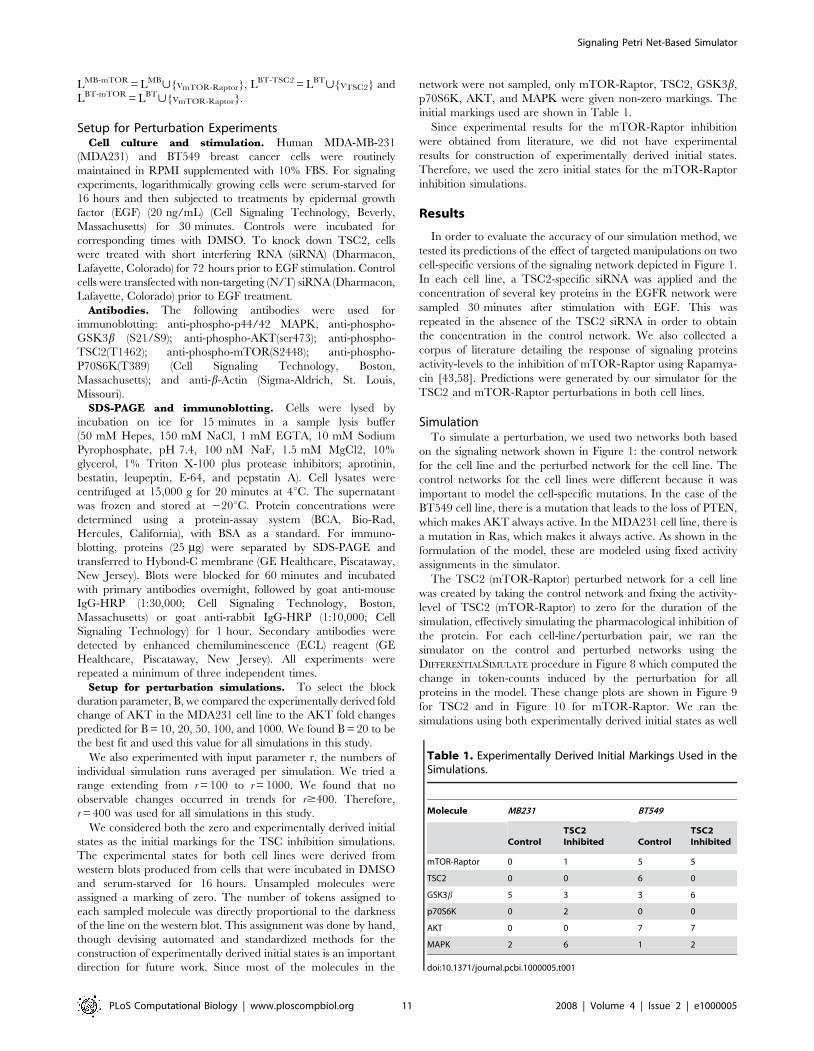
network were not sampled, only mTOR-Raptor, TSC2, GSK3b,

p70S6K, AKT, and MAPK were given non-zero markings. The

initial markings used are shown in Table 1.

Since experimental results for the mTOR-Raptor inhibition

were obtained from literature, we did not have experimental

results for construction of experimentally derived initial states.

Therefore, we used the zero initial states for the mTOR-Raptor

inhibition simulations.

Results

In order to evaluate the accuracy of our simulation method, we

tested its predictions of the effect of targeted manipulations on two

cell-specific versions of the signaling network depicted in Figure 1.

In each cell line, a TSC2-specific siRNA was applied and the

concentration of several key proteins in the EGFR network were

sampled 30 minutes after stimulation with EGF. This was

repeated in the absence of the TSC2 siRNA in order to obtain

the concentration in the control network. We also collected a

corpus of literature detailing the response of signaling proteins

activity-levels to the inhibition of mTOR-Raptor using Rapamya-

cin [43,58]. Predictions were generated by our simulator for the

TSC2 and mTOR-Raptor perturbations in both cell lines.

SimulationTo simulate a perturbation, we used two networks both based

on the signaling network shown in Figure 1: the control network

for the cell line and the perturbed network for the cell line. The

control networks for the cell lines were different because it was

important to model the cell-specific mutations. In the case of the

BT549 cell line, there is a mutation that leads to the loss of PTEN,

which makes AKT always active. In the MDA231 cell line, there is

a mutation in Ras, which makes it always active. As shown in the

formulation of the model, these are modeled using fixed activity

assignments in the simulator.

The TSC2 (mTOR-Raptor) perturbed network for a cell line

was created by taking the control network and fixing the activity-

level of TSC2 (mTOR-Raptor) to zero for the duration of the

simulation, effectively simulating the pharmacological inhibition of

the protein. For each cell-line/perturbation pair, we ran the

simulator on the control and perturbed networks using the

DIFFERENTIALSIMULATE procedure in Figure 8 which computed the

change in token-counts induced by the perturbation for all

proteins in the model. These change plots are shown in Figure 9

for TSC2 and in Figure 10 for mTOR-Raptor. We ran the

simulations using both experimentally derived initial states as well

Table 1. Experimentally Derived Initial Markings Used in theSimulations.

Molecule MB231 BT549

ControlTSC2Inhibited Control

TSC2Inhibited

mTOR-Raptor 0 1 5 5

TSC2 0 0 6 0

GSK3b 5 3 3 6

p70S6K 0 2 0 0

AKT 0 0 7 7

MAPK 2 6 1 2

doi:10.1371/journal.pcbi.1000005.t001



as zero initial states. The initial state used did not change the

overall trends observed in the simulations.

Using the t-test described in the Methods section, we also

computed the statistical significance of the final time block (b = 20)

for each molecule considered. For each molecule considered, 400

runs, 20 time blocks, and 50 samples were used. With the

exception of GSK3b which did not show a significant response to

the perturbation, the changes of all other proteins sampled were

beyond the 0.05 significance level (see Table 2). The statistical

insignificance of the change in GSK3b is not surprising since, as

shown in Figure 1, GSK3b is solely activated by LKB, a molecule

fixed high in both cell lines. Thus, we should not expect either

perturbation to have a significant effect on the activity of GSK3b,

which is what the t-value indicates.

Experimental ResultsAfter the TSC2 perturbation was applied to a cell line, the

protein concentrations were collected using western blots. Details

are given in the Materials and Methods section. The western blot

results are shown in Figure 9.

Discussion

As can be seen in Table 3, our method correctly predicted the

relative protein activity-level changes induced by the TSC2

perturbation in both cell lines, for most molecules sampled.

Notice that no change (–) was reported for the predicted response of

MAPK to the TSC2 perturbation despite the fact that a small

change did occur in its marking during the simulation (see Figure 9)

Figure 9. The Results of the TSC2 Perturbation Experiments and Simulations. In the western blots, columns (or lanes) are as follows: (1)non-targeting (NT) control siRNA, (2) NT siRNA+EGF, (3) TSC2 siRNA, (4) TSC2 siRNA+EGF. The effect of the TSC2 siRNA on a given molecule can beassessed by comparing column 4 against column 2. For each molecule in the western blot, there is a corresponding simulation curve showing thepredicted change in protein activity over time. For the purposes of this analysis, we compared the concentration change after 20 time steps (the left-most data points in the plots) for each molecule. Each simulation point corresponds to the average of 400 measurements that were computed usingthe procedure described in Figure 8. Experimentally derived initial states were used in the simulations. The results of both the experiments andsimulations are qualitatively summarized in Table 3.doi:10.1371/journal.pcbi.1000005.g009



and the t-value for the change is significant (see Table 2). At first,

interpreting this value as no change may seem misleading. However,

one of the significant challenges in experimental perturbation

experiments is separating true system responses from the

background noise created by experimental variables that cannot

be precisely controlled (among them cell population sizes,

variability in microarray antibody binding effectiveness, and

limited sensitivity of hardware and software used to quantify

experimental results). As a result, a common practice is to only

consider those substantial changes that are well beyond the

background noise level. Our interpretation of the small predicted

change in MAPK as no change reflects the fact that such small

changes would not be detectable in microarray or western blot

results. Thus, though such a small fluctuation might have occurred

in the real data, it would not have been detected by the biologists

and most likely would appear in the experimental data to have not

changed.

Similar reasoning guided our decision to characterize the

simulation (and experimental) results as either up (q), down (Q),

or no change (2) in general. Since the amount of protein

registered in a microarray or western blot is not always a reliable

indicator of the exact amount of protein (or protein form) being

measured, biologists are often reluctant to report degrees of

increases or decreases—preferring binary observations such as up

or down which are less subject to influence by extraneous

experimental conditions. It is true that our simulation method

produces precisely quantified increases or decreases which can be

taken to indicate degrees of change in response to perturbations.

However, as experimental techniques cannot reliably measure

degrees of increase or decrease, we judged the binary (up or down)

characterization to be a more reliable way of validating our

method. Certainly, our method provides additional information of

Figure 10. The Predicted Response of the Network to an mTOR-Raptor Perturbation. The predicted response of the network to a mTOR-Raptor perturbation in the (A) MDA231 and (B) BT549 cell lines. Our method predicts that the amount of available AKT increases in response to theperturbation, which is in agreement with results published in the literature [43,58]. Our method also predicts that the activity-level of p70S6K in theMDA231 cell line decreases in response to the perturbation, which has been observed experimentally [59]. Each point corresponds to the average of400 measurements that were computed using the procedure described in Figure 8.doi:10.1371/journal.pcbi.1000005.g010

Table 2. The T-Values for the Molecules Sampled in theMicroarray.

Molecule t-Value in MDA231 t-Value in BT549

mTOR-Raptor 41.72 30.53

TSC2 21.65 8.28

GSK3b 0.42 0.10

p70S6K 14.22 5.83

AKT 6.60 9.55

MAPK 16.35 18.93

The critical value for an alpha value of 0.05 with 50 samples is 2.0086. Note thatthe t-values for all molecules except for GSK3b are larger than this value,confirming that these changes are statistically significantly.doi:10.1371/journal.pcbi.1000005.t002

Table 3. Summary of the Effect of Perturbation Reported byExperimental and Simulated Methods.

Molecule MB231 BT549

Experiment Simulation Experiment Simulation

mTOR-Raptor q q q or 2 q

TSC2 Q Q Q Q

GSK3b 2 2 2 2

p70S6K q q Q q

AKT Q or 2 Q Q Q

MAPK 2 2 2 2

The up arrow (q) indicates that the perturbation caused a rise in the level ofthe phosphorylated protein; the straight line (2) indicates no change; and thedown arrow (Q) indicates that a decrease occurred. Values in the Experimentcolumn were estimated by comparing lanes 4 and 2 in Figure 9. We estimatedthe Simulation column by determining whether the top quartile of thedistribution for the final time point was above, below, or at zero. In some casesit is difficult to judge for certain whether the total quantity of thephosphorylated protein changed or remained the same—both for theexperimental and computational cases. In these situations, we indicated theuncertainty by listing the possible changes that the protein could have feasiblyundergone.doi:10.1371/journal.pcbi.1000005.t003



degrees of change and we consider studying the accuracy of these

degrees to be an important area for future work.

Our method also correctly predicted the activity-level change of

AKT in response to mTOR-Raptor inhibition as reported by a

number of studies [43,58]. Further, our method predicted that,

when mTOR-Raptor is inhibited, the level of p70S6K in the

MDA231 cell line decreased, which also had been observed

experimentally [59].

The only incorrect prediction made by our method was the

activity-level change of p70S6K in the BT549 cell line. However,

BT549 cells contain an RB mutation [49] which could alter

p70S6K phosphorylation [60]. It is a strength of our simulator that

the discrepancy between our method’s predictions and the

experimental results identified a section of the model in which

additional connectivity has been found which might account for

the difference observed.

The predictions made by our simulator would be exceedingly

difficult to derive by visual or manual inspection. Table 4 shows the

number of paths between several pairs of compounds within the

network. Where there is more than one path connecting two

molecules, feed forward and feed backward loops are present.

Attempting to determine, by hand, how these different loops will

interact with one another is, by itself, a difficult endeavor even when

not considering the additional task of deriving the rest of the network

dynamics simultaneously. For the larger networks that are now

becoming available, computational analysis becomes even more

crucial to obtaining insights into the dynamic behavior of the network.

Despite the complexity of the network dynamics, it was

straightforward to find and integrate the connectivity information

used to build it. Most of the information sources [36–43]

established the existence of various pathways and provided few or

no biochemical or kinetic details. As a result, the literature we used

would have provided little assistance is building a parameterized

Petri net or ODE model. Due to the proliferation of curated

signaling network repositories and searchable literature archives,

connectivity information is relatively abundant which makes the

ad hoc assembly of networks a relatively straightforward endeavor.

This further underscores the advantage of using our method over

ODEs or parameterized Petri nets to quickly model and

characterize some of the dynamics of a signaling network.

For simulations that will be compared to experimental results, the

time parameter must be selected carefully. The time parameter, B,

indicates how many time blocks our method will simulate. The time

block is an abstract unit of time. Therefore, before comparing

experimental results and predictions, it is necessary to determine how

many seconds, minutes, or hours correspond to a time block. This

can be done by comparing a prediction of the simulator with the

experimentally measured activity-level of one or two proteins at

several time points in order to determine what time blocks

correspond to the different sampled time points. In the present

study, we calibrated our time blocks only once for two cell lines and

six experimental conditions (two cell lines, with/without TSC2,

with/without mTOR-Raptor). To select the time parameter we used

the experimentally measured activity changes in two proteins at two

time points. In contrast to other predictive dynamic analysis tools

which require multiple time points and multiple protein samples in

order to calibrate simulation and model parameters, our method has

relatively low time and resource investment.

Besides the time parameter, the other component of our

simulations which involved experimentally obtained knowledge

was the initial states. The experimentally derived initial states

require that some experimental data be available providing

information on the initial concentrations of individual signaling

proteins in the network prior to stimulation. However, in the

network that we considered here, the overall behavior of the

network and of individual signaling proteins was resilient to

changes in the initial states used. Zero and experimentally derived

both produced the same overall change predictions. Thus, while

experimentally derived initial states may be important for the

simulation of some networks, it may well be the case that many

networks (such as the one we considered in this paper) can be

simulated without this knowledge—further reducing the experi-

mental work that must be done prior to simulation.

The fact that our simulator produced accurate predictions for a

variety of experimental conditions using the one core network

model and set of simulation parameters also distinguishes our

method from other predictive approaches. The only aspects of the

model that were modified during the simulations were activity-

levels reflecting the immediate effects of either the underlying

tumor mutations (Ras and PTEN) or the perturbations (mTOR-

Raptor and TSC2 targeted manipulation). In contrast, the

accuracy of ODEs and Petri nets predictions are known to be

sensitive to small changes to the model. For comparative studies

such as the one conducted in this paper, an ODE or

parameterized Petri net model might need to be re-constructed

with different parameters for each experimental condition of

interest. As a result, while it is possible to obtain our simulation

results using these models, it remains beyond the capabilities of

any existing ODE or parameterized Petri net system to provide

insights into the effects of experimental conditions on the dynamic

behavior of a signaling network with so little initial time and

resource investment.

Though our method’s predictions will not be as accurate as the

results returned by a correctly parameterized ODE, biologists

using our method can derive information about a network’s

dynamic behavior without having to conduct extensive experi-

mentation and computationally expensive parameter estimation.

This novel capability offers scientists the exciting prospect of being

able to test hypotheses regarding signal propagation in silico. As a

result, by using our method researchers can evaluate a wide array

of network responses in order to determine the most promising

experiments before even entering the laboratory.

Acknowledgments

We gratefully acknowledge the three anonymous reviewers, whose

comments and feedback improved the manuscript significantly.

Author Contributions

Conceived and designed the experiments: DR MM JTT PTR. Performed

the experiments: DR MM JTT. Analyzed the data: DR MM LN PTR.

Contributed reagents/materials/analysis tools: DR MM LN PTR. Wrote

the paper: DR MM LN PTR.

Table 4. Number of Paths Connecting Several Pairs ofCompounds in the EGFR Model Used in Our Simulations

Source Protein Destination Protein Number of Paths

EGFR TSC2 7

AKT mTOR-Raptor 6

MEK EGFR 4

AKT p70S6K 8

The multiple paths connecting pairs of proteins highlight the complexinteractions present within the network that give rise to its overall dynamicbehavior.doi:10.1371/journal.pcbi.1000005.t004



References

1. Hunter T (2000) Signaling-2000 and beyond. Cell 100: 113–127.

2. Hanahan D, Weinberg RA (2000) The Hallmarks of Cancer. Cell 100: 57–70.3. Feldman DS, Carnes CA, Abraham WT, Bristow MR (2005) Mechanisms of

Disease: beta-adrenergic receptors alterations in signal transduction andpharmacogenomics in heart failure. Nature Clinical Practice Cardiovascular

Medicine 2: 475–483.

4. Belloni E, Muenke M, Roessier E, Traverse G, Siegel-Bartelt J, et al. (1996)Identification of Sonic hedgehog as a candidate gene responsible for holopro-

sencephaly. Nat Genet 14: 353–356.5. Ma’ayan A, Jenkins SL, Neves S, Hasseldine A, Grace E, et al. (2005) Formation

of regulatory patterns during signal propagation in a Mammalian cellular

network. Science 309: 1078.6. Papin JA, Hunter T, Palsson BO, Subramaniam S (2005) Reconstruction of

cellular signalling networks and analysis of their properties. Nat Rev Mol CellBiol 6: 99–111.

7. The Cancer Cell Map (2006) http://cancer.cellmap.org/cellmap/.8. Kanehisa M, Goto S (2000) KEGG: Kyoto Encyclopedia of Genes and

Genomes. Nucleic Acids Res 28: 27–30.

9. Thomas PD, Campbell MJ, Kejariwal A, Mi J, Karlak B, et al. (2003)PANTHER: a library of protein families and subfamilies indexed by function.

Genome Res 13: 2129–2141.10. Dasika MS, Burgard A, Maranas CD (2006) A computational framework for the

topological analysis and targeted disruption of signal transduction networks.

Biophysical J 91: 382–398.11. Eker S, Knapp M, Laderoute K, Lincoln P, Talcott C (2002) Pathway Logic:

Executable Models of Biological Networks. Electronic Notes TheoreticalComputer Science 71.

12. Ruths D, Nakhleh L, Iyengar MS, Reddy SAG, Ram PT (2006) Graph-theoreticHypothesis Generation in Biological Signaling Networks. J Computational

Biology 13: 1546–1557.

13. Schaub MA, Henzinger TA, Fisher J (2007) Qualitative networks: a symbolicapproach to analyze biological signaling networks. BMC Systems Biology 1: 4.

14. Papin JA, Palsson BO (2004) The JAK-STAT signaling network in the humanB-cell: an extreme signaling pathway analysis. Biophysical J 87: 37–46.

15. Papin JA, Price ND, Wiback SJ, Fell DA, Palsson BO (2003) Metabolic

pathways in the post-genomic era. Trends Biochemical Sciences 28: 250–258.16. Schilling CH, Letscher D, Palsson BO (2000) Theory for the Systemic Definition

of Metabolic Pathways and their use in Interpreting Metabolic Function from aPathway-Oriented Perspective. J Theoretical Biology 203: 229–248.

17. Chaouiya C (2007) Petri net modelling of biological networks. BriefingsBioinformatics 8: 210–219.

18. Li C, Suzuki S, Nakata M (2006) Structural Modeling and Analysis of Signaling

Pathways Based on Petri Nets. J Bioinformatics Computational Biology 4:1119–1140.

19. Sackmann A, Heiner M, Koch I (2006) Application of Petri net based analysistechniques to signal transduction pathways. BMC Bioinformatics 7: 482–498.

20. Steggles LJ, Banks R, Shaw O, Wipat A (2007) Qualitatively modelling and

analysing gene regulatory networks: a Petri net approach. Bioinformatics 23:336–343.

21. Bhalla US, Ram PT, Iyengar R (2002) MAP kinase phosphatase as the locus offlexibility in a mitogen-activated protein kinase signaling network. Science 297:

1018–1023.22. Bornheimer SJ, Maurya MR, Farquhar MG, Subramaniam S (2004)

Computational modeling reveals how interplay between components of a

GTPase-cycle module regulates signal transduction. Proc Natl Acad Sci U S A101: 15899–15904.

23. Hoffman A, Levchenko A, Scott ML, Baltimore D (2002) The IkB-NF-kBsignaling module: temporal control and selective gene activation. Science 298:

1242–1245.

24. Huang CY, Ferrell JE (1996) Ultrasensitivity in the mitogen-activated proteinkinase cascade. Proc Natl Acad Sci U S A 93: 10078–10083.

25. Ferrell JE, Machleder EM (1998) The biochemical basis of an all-or-none cellfate switch in Xenopus oocytes. Science 280: 895–898.

26. Bailey JE (2001) Complex biology with no parameters. Nat Biotechnol 19:

503–504.27. Novere NL, Finney A, Hucka M, Bhalla US, Campagne F, et al. (2005)

Minimum information requested in the annotation of biochemical models(MIRIAM). Nat Biotechnol 23: 1509–1515.

28. Arisi I, Cattaneo A, Rosato V (2006) Parameter estimate of signal transductionpathways. BMC Neuroscience 7: S6.

29. Doi A, Fujita S, Matsuno H, Nagasaki M, Miyano S (2004) Constructing

Biological Pathway Models with Hybrid Functional Petri Nets. In Silico Biology4: 271–291.

30. Hardy S, Robillard PN (2004) Modeling and Simulation of Molecular BiologySystems using Petri Nets: Modeling Goals of Various Approaches.

J Bioinformatics Computational Biology 2: 619–637.

31. Matsuno H, Tanaka Y, Aoshima H, Doi A, Matsui M, et al. (2003) Biopathways

representation and simulation on hybrid functional Petri net. In Silico Biology 3:389–404.

32. Li S, Assmann SM, Albert R (2006) Predicting essential components of signaltransduction networks: a dynamic model of guard cell abscisic acid signaling.

PLoS Biology 4: e312–e328.

33. Glass L, Kauffman A (1973) The logical analysis of continuous non-linearbiochemical control networks. J Theoretical Biology 39: 103–129.

34. Jong HD, Geiselmann J, Batt G, Hernandez C, Page M (2004) QualitativeSimulation of the Initiation of Sporulation in Bacillus subtilis. Bull Mathematical

Biology 66: 261–299.

35. Muller M, Obeyesekere M, Mills GM, Ram PT (2007) Network topologydetermines dynamics of the mammalian MAPK1,2 signaling network: bi-fan

motif regulation of C-Raf and B-Raf isoforms by FGFR and MC1R. FASEB J;In press.

36. Avruch J, Hara K, Lin Y, Liu M, Long X, et al. (2006) Insulin and amino-acidregulation of mTOR signaling and kinase activity through the Rheb GTPase.

Oncogene 25: 6361–6372.

37. Inoki K, Ouyang H, Zhu T, Lindvall C, Wang Y, et al. (2006) TSC2 integratesWnt and energy signals via a coordinated phosphorylation by AMPK and GSK3

to regulate cell growth. Cell 126: 955–968.38. Karbowniczek M, Cash T, Cheung M, Robertson GP, Astrinidis A, et al. (2004)

Regulation of B-Raf kinase activity by tuberin and Rheb is mTOR-independent.

J Biological Chemistry 279: 29930–29937.39. Kwiatkowski DJ, Manning BD (2005) Tuberous sclerosis: a GAP at the

crossroads of multiple signaling pathways. Human Molecular Genetics 14:R251–R258.

40. Liang J, Shao SH, Xu ZX, Hennessy B, Ding Z, et al. (2007) The energy sensingLKB1-AMPK pathway regulated p27(kip1) phosphorylation mediating the

decision to enter autophagy or apoptosis. Nature Cell Biology 9: 218–224.

41. Ma L, Chen Z, Erdjument-Bromage H, Tempst P, Pandolfi PP (2005)Phosphorylation and functional inactivation of TSC2 by Erk implications for

tuberous sclerosis and cancer pathogenesis. Cell 121: 179–193.42. Manning BD, Logsdon MN, Lipovsky AI, Abbott D, Kwiatkowski DJ, et al.

(2005) Feedback inhibition of Akt signaling limits the growth of tumors lacking

Tsc2. Genes and Development 19: 1773–1778.43. O’Reilly KE, Rojo F, She QB, Solit D, Mills GB, et al. (2006) mTOR inhibition

induces upstream receptor tyrosine kinase signaling and activates Akt. CancerResearch 66: 1500–1508.

44. David R, Alla H (2005) Discrete, Continuous, and Hybrid Petri Nets. Springer.45. Aldana M, Cluzel P (2003) A natural class of robust networks. Proc Natl Acad

Sci 100: 8710–8714.

46. Kauffman S, Peterson C, Samuelsson B, Troein C (2004) Genetic networks withcanalyzing Boolean rules are always stable. Proc Natl Acad Sci 101:

17102–17107.47. Klemm K, Bornholdt S (2005) Topology of biological networks and reliability of

information processing. Proc Natl Acad Sci U S A 102: 18414–18419.

48. Chaves M, Albert R, Sontag ED (2005) Robustness and fragility of Booleanmodels for genetic regulatory networks. J Theoretical Biology 235: 431–449.

49. Neve RM, Chin K, Fridlyand J, Yeh J, Baehner FL, et al. (2006) A collection ofbreast cancer cell lines for the study of functionally distinct cancer subtypes.

Cancer Cell 10: 515–527.50. Bray D (1995) Protein molecules as computational elements in living cells.

Nature 376: 307–312.

51. Iyengar R, Birnbaumer L, editors (1989) G Proteins. New York: Academic Press.52. Jordan JD, Landau EM, Iyengar R (2000) Signaling networks: the origins of

cellular multitasking. Cell 103: 193–200.53. Eungdamrong NJ, Iyengar R (2004) Modeling cell signaling networks. Biology

Cell 96: 355–362.

54. Eungdamrong NJ, Iyengar R (2004) Computational Approaches for modelingregulatory cellular networks. Trends Cell Biology 14: 661–669.

55. Gianchandani EP, Brautigan DL, Papin JA (2006) Systems analyses characterizeintegrated functions of biochemical networks. Trends Biochemical Sci 31:

284–291.

56. Blinov ML, Faeder JR, Goldstein B, Hlavacek WS (2006) A network model ofearly events in epidermal growth factor receptor signaling that accounts for

combinatorial complexity. BioSystems 83: 136–151.57. Inoki K, Corradetti MN, Guan KL (2005) Dysregulation of the TSC-mTOR

pathway in human disease. Nat Genet 37: 19–24.58. Sarbassov DD, Ali SM, Sabatini DM (2005) Growing roles for the mTOR

pathway. Curr Opin Cell Biol 17: 596–603.

59. Chen Y, Rodrik V, Foster DA (2005) Alternative phospholipase D/mTORsurvival signal in human breast cancer cells. Oncogene 24: 672–679.

60. Makris C, Voisin L, Giasson E, Tudan C, Kaplan DR, et al. (2002) The Rb-family protein p107 inhibits translation by a PDK1-dependent mechanism.

Oncogene 21: 7891–7896.



Documents

The Signaling Petri Net-Based Simulator: A Non- …nakhleh/Papers/RuthsEtAl-PLoS08.pdf · Parametric Strategy for Characterizing the Dynamics of ... dynamics of signal flow through