THE SIMPLE REGRESSION MODEL Chapter 2 1. I. Outline 2 Simple linear regression model-used to explain one variable in terms of another. Model Assumptions

THE SIMPLE REGRESSION MODEL

Chapter 2

1

I. Outline2

Simple linear regression model-used to explain one variable in terms of another. Model Assumptions

OLS estimator-method of estimating effect of one variable on another. Compute estimator Statistical properties: Unbiasedness &

Variance Units of measurement

II. Simple Linear Regression (SLR)

3

Basic Idea: y and x are two variables want to explain y in terms of x; how y

varies with changes in x y: soybean crop, hourly wage, crime rate x: lbs of fertilizer, years of education, # of

police

SLR model: y = 0 + 1x + u

II. SLR Terminology (Variables)

y is called the: Dependent Variable Left-Hand Side Variable Explained Variable Regressand

x is called the: Independent Variable Right-Hand Side

Variable Explanatory Variable Regressor Covariate Control Variables

u represents all factors other than x that affect y u is called the:

Error term Disturbance Unobserved

component (by econometrician)

4

y = 0 + 1x + u

II. SLR Terminology (Parameters)

0 is the intercept or constant term Basic value for y when x=0

1 is the slope parameter Measures the relationship between y and x Tells us how y changes when x changes by some

amount How to isolate this effect?

Δy = 1Δx if Δu=0 ceteris paribus: holding other factors fixed

5

y = 0 + 1x + u

II. SLR Examples

Example 1: Soybeans y: soybean yield x: fertilizer (lbs) u: land quality, rainfall Δyield=1Δfertilizer Measures change in

yield due to adding another unit of fertilizer…holds all other factors fixed

Example 2: Wages y: wage x: education (years) u: innate ability,

experience, work ethic Δwage=1Δeduc Measures change in

wage due to attaining another unit of education…holds all other factors fixed.

6

SLR model: y = 0 + 1x + u

II. SLR Notes7

SLR assumes linearity: y = 0 + 1x + u is equation for straight

line, where slope is constant A one unit change in x has the same effect

on y, regardless of initial value of x Example:

10th to 11th year of school has same impact on wage as going from 11th to 12th….may not be realistic.

Will consider more realistic forms later…

II. SLR AssumptionsSimplifying Assumption: Mean Zero Error

8

The average value of u, the error term, in the population is 0. Terminology: Expectation is just finding the average

E(u) = 0 Ex: average ability is zero, average land quality is

zero.

This is not a restrictive assumption, since we can always use 0 to normalize E(u) to 0 y = 0 + 1x + u +α0 - α0, where α0 is E(u) y = (α0 + 0 )+ 1x + (u - α0 )….1 is not affected.

n

iiz

nzE

1

*1

)(

II. SLR AssumptionsMore Important Assumption: Zero Conditional Mean

9

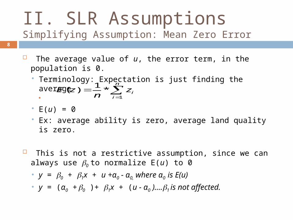
In order for 1 to estimate only the effect of x on y, we need to make a crucial assumption about how u and x are related.

Average value of u does not depend on the value of x. Terminology:

Conditioning on a variable w means we use values of w to explain values of z: E(z|w).

If w does not tell us anything about z, E(z|w)=E(z). Note: E(z|w)=E(z) implies Cov(z, w)=0

E(u|x)=E(u) Knowing something about x does not give us any information about u…

implies x and us are completely unrelated.

II. SLR Assumptions:More Important Assumption: Zero Conditional Mean

10

Example: Wage equation: wage = 0 + 1educ + u let u represent unobserved ability

E(u|educ) requires that average ability is the same regardless of years of education E(ability|educ=12)=E(ability|educ=16)

How likely is this? Generally think people that choose to get more

education are more able. E(ability|educ=12)<E(ability|educ=16).

II. SLR Assumptions11

Combining the two assumptions: E(u|x) = E(u) = 0

Taking the expectation of both sides of SLR model: E(y|x)=E(0 + 1x + u |x)….

E(y|x)=E(0 |x)+ E(1x |x) + E(u|x)….

E(y|x) = 0 + 1x

Called the Population Regression Function Now y is written only in terms of x…. this allows us to

identify impact of x on y. Note: Above derivation used multiple properties of E(.),

including linear operator, conditioning on a constant, conditioning on variable itself (see Appendix A-C)

III. Ordinary Least Squares (OLS)

12

Basic Idea: Take SLR model and estimate parameters of

interest using a sample of data OLS is a method for estimating the parameters

Data: Let {(xi,yi): i=1, …,n} denote a random sample

of size n from the population Model: For each observation we can write:

yi = 0 + 1xi + ui

y = 0 + 1x + u (vector notation)

Copyright © 2009 South-Western/Cengage Learning 13

III. Deriving OLS Estimates14

To derive the OLS estimates, we need use the SLR assumptions: E(u)=0 and E(u|x)=E(u)….E(u|x)=E(u)=0 Recall, this means Cov(u,x)=0

Covariance is a measure of the linear dependence between two variables

Using definition of covariance: Cov(u,x) =0= E(xu)-E(x)E(u) =E(xu)

So now we have that: E(u)=0 E(ux)=0

III. Deriving OLS Estimates (continued)

15

We can write our 2 restrictions just in terms of x, y, 0 and , since u = y – 0 – 1x E(u)=0……..E(y – 0 – 1x) = 0 E(xu)=0……E[x(y – 0 – 1x)] = 0

These restrictions are often called moment restrictions or first order conditions.

It is important to note that we have 2 equations, 2 unknowns so we have an exactly identified system of equations.

OLS finds so that these equations are satisfied. “hats” denote that we are talking about estimates

^

1

^

0 ,


Step 1: We know E(.) is just the mean, so the sample counterparts to the two moment equations are (at the estimated parameters):

0ˆˆ

0ˆˆ

110

1

110

1

n

iiii

n

iii

xyxn

xyn

16


Step 2: Using the following algebraic properties, and similarly for x Summation is linear operator

we can rewrite the first moment as:

17

n

iiyny

1

1

xy 10ˆˆ

0ˆˆ1

101

n

iii xyn

xy 10ˆˆ


18

Step 3: Substituting this into the second moment condition:

Note: Dropping n-1doesn’t affect the estimation. Note: Above derivation uses the following

properties of summation:

n

iii

n

ii

n

iii

n

iii

n

iiii

xxyyxx

xxxyyx

xxyyx

1

21

1

11

1

111

ˆ

ˆ

0ˆˆ

n

iii

n

iii

n

ii

n

iii

yyxxyyx

xxxxx

11

1

2

1

))(()(

)()(


19

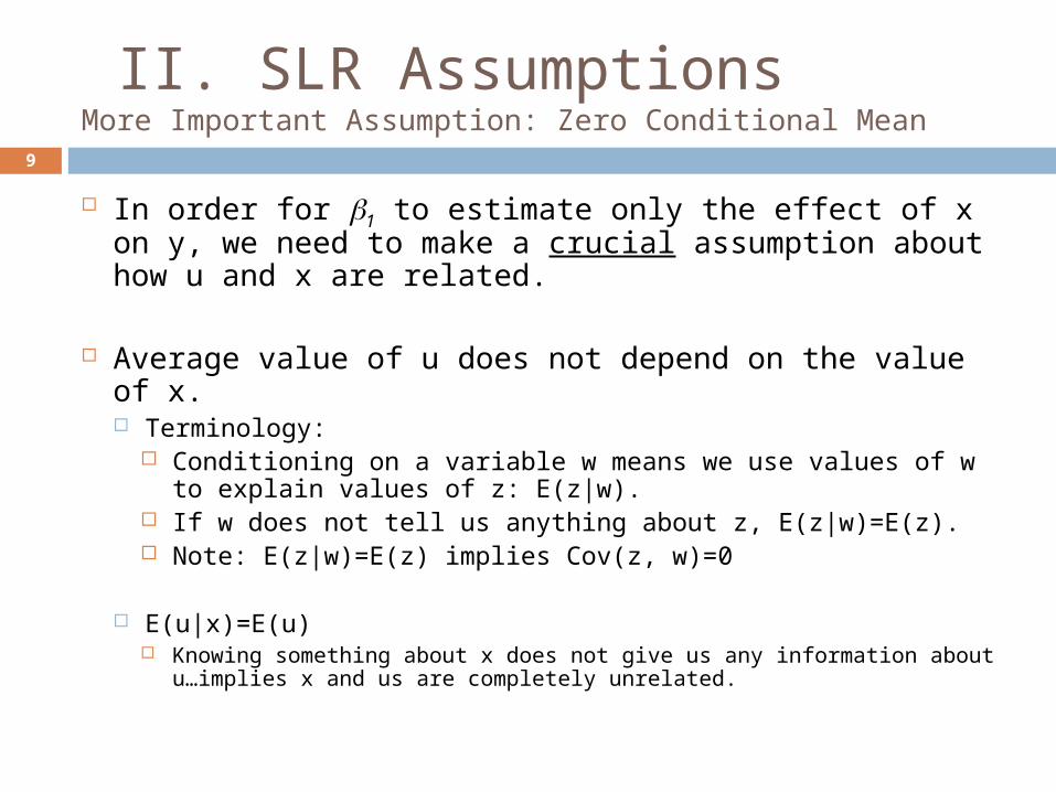
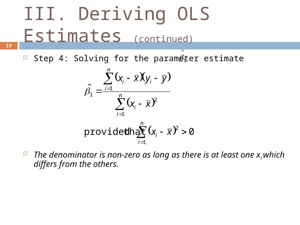
Step 4: Solving for the parameter estimate

The denominator is non-zero as long as there is at least one xi which differs from the others.

^

1

0 that provided

ˆ

1

2

1

2

11

n

ii

n

ii

n

iii

xx

xx

yyxx

III. Summary of OLS slope estimate

20

The slope estimate is the sample covariance between x and y divided by the sample variance of x. Variance: Measure of spread in the distribution of a

random variable Covariance: Measure of linear dependence between two

random variables.

If x and y are: positively correlated, the slope will be positive negatively correlated, the slope will be negative

III. Deriving OLS EstimatesAlternative Approach

21

Intuition on OLS: Are fitting a line through the sample points (xi,yi) Claim: Are defining line of “best fit” such that the

sum of squared residuals is as small as possible What is a residual?

Residual is the estimate of the error term:

Minimization problem: 110

^^^ˆˆ where, xyyyu

n

iii

n

ii xyu

1

2

101

2 ˆˆˆ

III. Deriving OLS EstimatesAlternative Approach

To solve the minimization problem we need to take first order conditions. For each parameter:

These first order conditions are the same as the moment conditions, multiplied by n-1

OLS finds the parameters that best solve these equations.

Leads to name least squares estimator

0ˆˆ

0ˆˆ

110

110

n

iiii

n

iii

xyx

xy

22

23

.

..

.

y4

y1

y2

y3

x1 x2 x3 x4

}

}

{

{

x

y

Sample OLS Line of Best Fit

^^

1

^

0)|(

Function Regression Sample

yxxyE

^

1u

^

2u

^

3u

^

4u

0

0

0

^

^

^

i

i

i

u

u

u

^^

1 x

y

IV. Properties of OLS Algebraic

24

The sum of the OLS residuals is zero:

The sample average of the OLS residuals is zero as well:

The sample covariance between the regressors and the OLS residuals is zero:

The OLS regression line always goes through the mean of the sample:

n

iiu

1

^

0

01

1

^

n

iiu

n

01

1

^

i

n

ii xu

n

xy 10

IV. Properties of OLS Algebraic

25

We can think of each observation yi as being composed of 2 parts: explained and unexplained

Can define the following: SST: SSE: SSR:

Total variation in y is expressed as the sum of the explained variation plus the unexplained variation. SST=SSE+SSR

0),cov( where,^^^^

iiiii uyuyy

(SSR) squares of sum residual theis ˆ

are ˆout spread how measures squares; of sum explained theis ˆ

are yout spread how measures :squares of sum total theis

2

2

i2

i

ii

i

u

yyy

yy

IV. Proof that SST = SSE + SSR

26

0 ˆˆ and ˆ that know weand

SSE ˆˆ2 SSR

ˆˆˆ2ˆ

ˆˆ

ˆˆ

22

2

22

yyuyy

yyu

yyyyuu

yyu

yyyyyy

ii

ii

iiii

ii

iiii

IV. Goodness-of-Fit27

Use these definitions to measure how well our independent variable explains the dependent variable.

Compute the fraction of the total sum of

squares (SST) that is explained by the model

R2 = SSE/SST = 1 – SSR/SST Aka coefficient of determination Measures fraction of variation in y that’s explained

by variation in x….between 0 and 1…smaller number indicates poorer fit.

Often multiply by 100%.

V. Examples: CEO Salary & Return on Equity

28

Regression specification Model:

Salary=0 + 1 *ROE + u “Regress salary on ROE”

Data: Salary is in thousands of $, so that 856.3 means

$856,300 ROE is in percentages

Parameter: 1 measures the change in annual salary (in

thousands of $), when ROE increases by 1% point (one unit)

Copyright © 2009 South-Western/Cengage Learning

29

V. Examples: CEO Salary & Return on Equity

30

Results: Sample Regression Function: If ROE=0, then predicted salary is 963.51…$963,510 Slope Estimate:

If ROE increases by 1% point, then salary is predicted to change by 18.501…$18,500

Linearity imposes that the predicted salary change is 18.501 regardless of initial ROE.

ROE=20, then predicted salary is $1,333,215 …in reality, actual salary is $1,145,000.

R2 =0.0132 from regression: variation in ROE explains 1.3% of variation in salary

ROEsalary *501.1851.963^

ROEsalary *501.18^


31

V. Examples:

Regression results: Data

Wage: $ per hour Educ: years of education

Negative wage for person with no education implies regression line does bad job at low levels of educ.

Predicted wage for 8 years is $3.42= -0.90+0.54*8

Increase in education by 1 year (unit) leads to increase in hourly wage by $0.54…increase by 4 years leads to $0.54*4=$2.16

Is it reasonable that each extra year leads to same wage increase?

educwage *54.090.0^

32

Wage & Education Voting Outcomes & Expenditure

Regression results: Data

voteA: % of vote received by A

shareA: % of total campaign expenditures accounted for by A.

If candidate A’s share of spending increases by 1% point (unit), that candidate will receive 0.464% more votes.

shareAvoteA *464.081.26^

VI. Properties of OLS EstimatorUnbiasedness33

One key statistical property of the OLS estimator is that it gives us unbiased estimates, , of the parameters Unbiased estimates:

Intuition: We only have a single sample to estimate , and so the

estimates we get may or may not be equal to the true parameter.

If we had multiple samples of data and in each, estimate , then the average of all these estimates should be equal to population parameter.

There are 4 assumptions that we must make to ensures unbiasedness.

11

^

00

^

)|(

)|(

xE

xE

10ˆ,ˆ 10 ,

10ˆ,ˆ

10ˆ,ˆ

VI. Properties of OLSUnbiasedness

34

SLR.1 Linear in Parameters Assume the population model is linear in

parameters as y = 0 + 1x + u I.e. we are estimating 0 and 1, not, say 1

SLR.2 Random Sampling Assume we have a random sample of size n,

{(xi, yi): i=1, 2, …, n}, from the population. This allows us to write the sample model yi

= 0 + 1xi + ui


35

SLR.3 Sample variation in x There is variation in x across i Var(x) ≠ 0

SLR.4 Zero Conditional Mean Most important for unbiasedness E(u|x) = 0 and thus E(ui|xi) = 0


To show unbiasedness, we first rewrite our OLS estimator

(recall: (App. A))

Using algebra:

2221

21 where,ˆ as ,

)(

)(ˆ xxss

yxx

xx

yyxxix

x

ii

i

ii

36

iiii yxxyyxx )())((

iiiii

iiiii

iiiii

uxxxxxxx

uxxxxxxx

uxxxyxx

10

10

10


37

We know that:

Let:

21

111

21

1 1

2

1

)(ˆ thusand ,)(

asrewritten becan numerator theso )()( and 0)(

x

n

iiin

iiix

n

i

n

iiii

n

ii

s

uxxuxxs

xxxxxxx

1211

211

|1|ˆ on x, ngconditioni Now,

.1ˆ that so ,

xuEds

xE

uds

xxd

iix

iix

ii


38

Can do the same for 0 (in text).

Unbiasedness is a description of the estimator. In any given sample of data, we may be “near” or

“far” from the true parameter (i.e. true effect of x on y)

Unbiasedness says that if have many estimates from many different samples, then, their average converges to the true parameter 1.

Proof of unbiasedness depends on our 4 assumptions If any assumption fails, then OLS is not necessarily

unbiased. Can slack on SLR.1 (out of scope of text) SLR.3 almost always holds

1

^


39

SLR. 2 can be relaxed when looking at time series data and panel data (later chapters). For cross-sectional data, assume SLR.2 holds

SLR.4 is most “crucial” assumption, and unfortunately the hardest to guarantee. As we saw with unobserved ability, it’s likely that x

is correlated with u. This can result in the OLS estimates reporting a

spurious or biased estimate of the effect of x on y estimating the effect of unobserved factors on y

because they are correlated with x.


40

Example: Student performance and National School Lunch Program (NSLP) Expect that, other factors being equal, a student

who receives a free lunch at school will have improved performance

Regression: 1 =-0.319, 0 =32.14 Indicates participation has negative effect on

achievement Likely that u (school quality, motivation) is

correlated with NSLP participation, meaning E(u) is different across participating and non-participating students.

ulunchprogtestscore 10

VII. Properties of OLSVariance

41

For a given sample of data, we estimate Even with unbiasedness, know our estimate is not

usually equal to the true parameter. Would like to know, on average, how far our estimate is

from the true parameter. Variance of an estimator How spread out the distributions of are. Measure of spread is the variance (or it’s square root,

standard deviation). Note: If had multiple methods of estimating the

parameters, would use this rubric to determine which is the best (i.e. lowest variance)

^

1

^

0 ,

^

1

^

0 ,


42

To calculate variance of an estimator, we first need to make a simplifying assumption: SLR.5 Homoskedasticity (constant variance) Var(u|x) = 2

Means the error term u has the same variance (spread) given any value of the explanatory variable.

Graphically…. Algebra:

Var(u|x) = E(u2|x)-[E(u|x)]2

We know E(u|x) = 0, so E(u2|x) = E(u2) = Var(u)=2

(this is a result of Var(u)=E(u2)-[E(u)]2 and E(u)=0) 2 is also the unconditional variance, called the error variance , the square root of the error variance is called the standard

deviation of the error

43

..

x1 x2

Homoskedastic Case

E(y|x) = 0 + 1x

y

f(y|x)

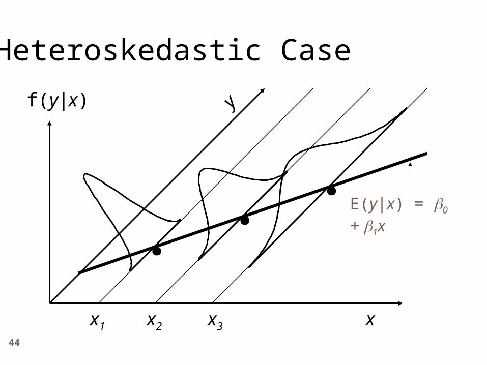
44

.

x x1 x2

yf(y|x)

Heteroskedastic Case

x3

..

E(y|x) = 0 + 1x


45

People often re-write SLR.4 and SLR.5 as SLR.4: E(u|x)=0

y =0 + 1x + u….E(y|x)=E(0 |x)+E(1x|x)+E(u|x) .…E(y|x)=0 + 1x

SLR.5: Var(u|x) = 2

Similarly, Var(u|x)=Var(y|x) = 2

Assuming homoskedasticity, we can derive an estimator for the variance of the OLS parameter estimates. Heteroskedasticity is more likely, but will ignore for now.

This will give us an idea of how precisely the parameter is estimated. Would like small variance, because this means our parameter

estimate is more likely to be close to the true value.


46

Calculating Variance of Estimator:

Properties: The larger the error variance, 2, the larger the variance

of the slope estimate…bad thing. The larger the variability in the xi, the smaller the

variance of the slope estimate (i.e. easier to pinpoint how y varies with x)…good thing. Consequently, a larger sample size should decrease the

variance of the slope estimate

)|ˆVar(for Similarly

B) (App. variancea of sum theis sum a of Variance :Note

)( 111

|1 x| 1| 1|ˆ

0

^

12

222

222

2

2222

2

2

22

2

2

2211

x

Vars

ss

ds

ds

xuVards

udVars

xuds

VarxVar

xx

xi

xi

x

iix

iix

iix


47

Calculating Error Variance: Recall 2 = E(u2) = Var(u) Problem: We don’t know what the error variance, 2, is

because we don’t observe the errors ui.

What we observe are the residuals, ûi

We can use the residuals to form an estimate of the error variance.

1100

101010

ˆˆ

ˆˆˆˆˆ

i

iiiiii

u

xuxxyu


48

Then, an unbiased estimator of 2 =E(u2) is:

We generally look at the spread of an estimator in terms of the standard error (estimate of standard deviation), which is the square root of the variance.

standard deviation: standard deviation:

2).-(n involvingestimator theuse weso here) discussed reasonsnot (for incorrect is but this

/ˆ1

ˆyieldst replacemen above thereality,In :Note

2/ˆ2

1ˆ

22

22

nSSRun

nSSRun

i

i

21

21 /ˆsd xxi

21

21 /ˆˆse xxi

VIII. Units of Measurement and Functional Form

49

We are essentially always trying to estimate the impact of x on y. The units for our variables will qualitatively affect how we

interpret the estimates…but, the punchline is the same. Example: CEO Salary and ROE

Model: Salary=0 + 1 *ROE + u

Data: Salary is measured in thousands of $, so that 856.3 means

$856,300 ROE is in %, so a one unit of change is 1%

Results: That is, when ROE increases by 1%, salary is predicted to increase

by 18.501 or $18,501

^

501.18*191.963 ROEsalary


50

Rule # 1: If dependent variable is multiplied by a constant c, then OLS intercept and slope estimates are also multiplied by c.

Rule # 2: If independent variable is divided (multiplied) by some non zero constant, c, then the OLS slope coefficient is multiplied (divided) by c. The intercept is not affected. Suppose ROE now measured as decimal…0.01 Results: When ROE increases by one unit (units are in decimals), this

means ROE changes by 0.01=1% : That is, when ROE changes by 0.01, salary is predicted to

increase by 1,850.1*0.01=18.501. Since salary is measured in thousands of $, this is a $18,501 increase.

ROEsalary *1.850,1191.963^

0.01ROE where,*1.850,1^

ROEsalary


51

Can incorporate nonlinearities in the variables to make our estimation more realistic.

Wage Example Estimate: Restricts each increase in a year of education to

have the same affect as the previous increase (10th to 11th, 11th to 12th both yield $0.54 increase).

This is unrealistic, as the 12th year culminates in a high school degree, and is likely rewarded in the labor market.

educwage *54.090.0^


52

An improvement would be to say that wage increases by a constant percentage at each additional year of education. Allows for the monetary impact of 10 to 11

to be different from 11 to 12, although the % increase is the same.

Model: Log(wage)= =0 + 1 *educ + u Using this form implies an increasing return

to education


53


54

Estimate: Log(wage)=0 + 1 *educ + u Results: Standard to multiply 1 *100% to get the

percentage change in wage given one additional unit (year) of schooling.

An extra year of education results in a 8.3% increase in predicted wage.

educwage *083.0584.0)log(^


55

What if our LHS and RHS are logs? Called Constant elasticity model Estimate: Log(wage)=0 + 1 log(sales)+ u Wage in $, sales in millions of $ 1 estimates the elasticity of salary with

respect to sales Result: Implies a 1% increase in firm sales

increases salary by 0.257%

)log(*257.0822.4)log(^

salessalary


56

Documents

THE SIMPLE REGRESSION MODEL Chapter 2 1. I. Outline 2 Simple linear regression model-used to explain one variable in terms of another. Model Assumptions